Embed Size (px)
Citation preview

Financial integration in the EMU:
The Fama and French Factors in the Euro zone
ERASMUS UNIVERSITY ROTTERDAM ERASMUS SCHOOL OF ECONOMICS MSc Economics & Business Master Specialisation Financial Economics
ERASMUS UNIVERSITY ROTTERDAM ERASMUS SCHOOL OF ECONOMICS MSc Economics & Business Master Specialisation Financial Economics
Author: H.W.C. Vreedenburgh Student number: 316308 Thesis supervisor: S. van Bekkum Finish date: July 2010
Author: H.W.C. Vreedenburgh Student number: 316308 Thesis supervisor: S. van Bekkum Finish date: July 2010

ii
PREFACE AND ACKNOWLEDGEMENTS I would like to thank my thesis supervisor Sjoerd van Bekkum for his useful comments, (fast) feedback
and keeping me challenged, even though he was in the United States, while I was writing this thesis.
This thesis has given me new knowledge and insights about asset pricing and the consequences of
integration for portfolio management. I found it very challenging and interesting to explore an area
which I did not know that much of.
The biggest and most time consuming challenge was the creation and error checking of the dataset, and
the creation of the portfolio for the 12 countries in Excel. However, I can now say I am quite adapt in
Excel.
Most importantly, I became very enthusiastic about the subject, motivating me to read a lot about
different aspects of the subject. This has resulted in the fact that I have learned a lot.
NON-PLAGIARISM STATEMENT By submitting this thesis the author declares to have written this thesis completely by himself/herself, and not to have used sources or resources other than the ones mentioned. All sources used, quotes and citations that were literally taken from publications, or that were in close accordance with the meaning of those publications, are indicated as such. COPYRIGHT STATEMENT The author has copyright of this thesis, but also acknowledges the intellectual copyright of contributions made by the thesis supervisor, which may include important research ideas and data. Author and thesis supervisor will have made clear agreements about issues such as confidentiality. Electronic versions of the thesis are in principle available for inclusion in any EUR thesis database and repository, such as the Master Thesis Repository of the Erasmus University Rotterdam
NON-PLAGIARISM STATEMENT By submitting this thesis the author declares to have written this thesis completely by himself/herself, and not to have used sources or resources other than the ones mentioned. All sources used, quotes and citations that were literally taken from publications, or that were in close accordance with the meaning of those publications, are indicated as such. COPYRIGHT STATEMENT The author has copyright of this thesis, but also acknowledges the intellectual copyright of contributions made by the thesis supervisor, which may include important research ideas and data. Author and thesis supervisor will have made clear agreements about issues such as confidentiality. Electronic versions of the thesis are in principle available for inclusion in any EUR thesis database and repository, such as the Master Thesis Repository of the Erasmus University Rotterdam

iii
ABSTRACT Integration in the EMU stock markets has some major implications for investors, their international
portfolio diversification possibilities and the way they should price stocks. This paper will add an
insight and provide evidence in the discussion whether or not the EMU stock market is can regarded as
an integrated market, and what this means for the way stocks should be priced.
This paper’s main contribution is providing evidence of EMU stock market integration by using a non-
correlation method and asset pricing models, and what asset pricing model is able to price the stocks
best in the integrated EMU zone.
Using the principal component analysis, we have shown that there is an increasing degree of integration
in the EMU zone. Although the rate of the smaller EMY countries is higher, the larger EMU countries
were already quite integrated.
This article also uses local, EMU and combined (EMU and local) factor models to see which model is
able to price EMU stocks as a way of testing integration. We show that the Fama and French three factor
model is better at pricing stocks for individual countries better than CAPM.
This article shows that the EMU factors are doing quite well on pricing stocks, especially in the larger
countries, although local factors still have an impact. Considering different time frames, we see that the
local factors have lost much of their additional explanatory power in the post-2001 period.
Finally, this paper shows that an EMU factor model is able to price all EMU stocks better than countries
individually.
Keywords: Asset pricing, Portfolio Choice, International Financial Markets, Financial Aspects of Economic Integration JEL: F36, G11, G12, G15

iv
Table of Contents PREFACE AND ACKNOWLEDGEMENTS .................................................................................................................................. ii
ABSTRACT .......................................................................................................................................................................................... iii
1 Introduction .............................................................................................................................................................................. 1
2 Background and prior research ........................................................................................................................................ 4
2.1 Background on the EMU and European Union. ................................................................................................ 4
2.2 Prior research and evidence for the integration of the EMU ...................................................................... 5
2.2.1 Integration in the EMU ...................................................................................................................................... 5
2.2.2 Implications of market integration in the EMU ...................................................................................... 7
2.3 Theoretical background on factor models .......................................................................................................... 8
2.3.1 The Capital Asset Pricing Model .................................................................................................................... 8
2.3.2 The Fama and French Three Factor Model ............................................................................................... 9
2.3.3 The rationale of the Fama and French factors ...................................................................................... 10
2.3.4 Critique on Fama and French ...................................................................................................................... 10
2.3.5 Extensions of the Three Factor Model ..................................................................................................... 11
3 Data set description ............................................................................................................................................................ 12
3.1 Data used ....................................................................................................................................................................... 12
3.2 Adding the ‘Dead Stock’ lists .................................................................................................................................. 13
3.3 Exchange and risk free rates ................................................................................................................................. 14
3.4 Inclusion or exclusion of stocks ........................................................................................................................... 14
4 Methodology .......................................................................................................................................................................... 15
4.1 Method to test for integration ............................................................................................................................... 15
4.2 Test for integration in the EMU area using the principal component analysis ................................ 17
4.3 Performance criteria for the principal component analysis .................................................................... 18
4.4 The factor models for testing integration ........................................................................................................ 19
4.4.1 The capital asset pricing model .................................................................................................................. 19
4.4.2 Fama and French three factor model for testing integration ......................................................... 19
4.4.3 Addition of international factors ................................................................................................................ 20
4.5 Performance criteria for the factor model ....................................................................................................... 21
5 Portfolio construction ........................................................................................................................................................ 22
5.1 Construction of the Fama and French risk factors ....................................................................................... 22
5.2 Construction the dependent variables portfolios ......................................................................................... 23
6 Empirical results of factor tests ..................................................................................................................................... 25
6.1 Statistics on the factors and portfolios .............................................................................................................. 25

v
6.1.1 General statistics ............................................................................................................................................... 25
6.1.2 Descriptive statistics ....................................................................................................................................... 26
6.1.3 Checking the factor results for robustness ............................................................................................ 27
6.2 Results on integration in the EMU using PCA ................................................................................................. 31
6.3 Results on the risk factors ...................................................................................................................................... 33
6.3.1 The ability of the local CAPM and the 3FM to price stocks ............................................................. 33
6.3.2 Measuring integration in the EMU zone .................................................................................................. 35
6.3.3 The factor models in the EMU over time ................................................................................................ 36
6.3.4 Pricing the EMU zone as a whole ............................................................................................................... 38
7 Conclusion .............................................................................................................................................................................. 40
7.1 Further research ......................................................................................................................................................... 42
8 Figures and Tables .............................................................................................................................................................. 45

1
1 Introduction
After the completion of the European Economic and Monetary Union (EMU), with the signing of the
Maastricht Treaty in 1992, and eventually the introduction of the euro in 1999, Europe is supposed to
have seen a remarkable economic integration ever since. As the euro was only introduced relatively
recently, there are still limited academic studies on what impact the EMU (and the introduction of the
euro) has on the EMU stock market, the integration of the EMU stock markets and its impact on stock
pricing alone.
Integration in the EMU equity markets has some major implications for investors, their international
portfolio diversification possibilities and the way they should price stocks.
This paper will add an insight and provide evidence in the discussion whether or not the EMU stock
market can be regarded as an integrated market, and what this means for the way stocks should be
priced.
This paper’s main contribution is providing evidence of EMU stock market integration by using a non-
correlation method and asset pricing models, and to show what asset pricing model is best to price the
stocks in the integrated EMU zone.
The structural changes in the financial markets of the EMU zone have resulted in a changing approach
to the use of EMU stocks in international portfolio management. An integrated European market could
have a major impact on the way investors price stocks and how to achieve a well-diversified portfolio.
Although the size of the EMU equity market is - compared to the United States- not that big in terms of
global market value, it has attracted a large number of non-EMU investors for its diversification
benefits.
These investors have looked for opportunities to reduce portfolio risk by investing in stocks across
different national markets where low correlations in return exist, while keeping the expecting return at
the same level.
However, the assumed integration process of the EMU zone could potentially limit these benefits, as
correlations between the EMU countries will rise. This could result in new optimizations in the
commonly used mean-variance frontier in modern portfolio theory (Markowitz, 1952) for investors in
the EMU zone.
On the other hand, the integration will lead to new opportunities and policies. The integration of the
EMU stock market could result in one big investment area instead of several different ones, resulting in
better risk sharing benefits, improvements in allocation efficiency and a reduction in economic volatility
(Baele et al., 2004).
The creation of the EMU made it also possible for investors to buy EMU stocks without any limitations,
as it is supposed to be a single market. Often, (institutional) investors were often restricted (for a

2
certain amount) to a certain country (or currency). This limitation could be removed if the EMU
appears to be actually one single market. This could result in more investments in the EMU zone.
It could also limit the question which EMU country is a better option, as the EMU zone will appear as
one investment opportunity, and shifts the question to which industry in the EMU is a better
investment.
In this paper we assume that the integration in the EMU market means that every stock within the EMU
countries is subject to same (financial) circumstances and sensitive to the same (financial) shocks,
regardless of the country in which they are traded. There should be no market frictions within the EMU
stock markets and EMU countries.
This means that every investor in the EMU has the same opportunity set, the same limitations, same
costs and risks when investing in stocks. We consider this as a fair expectation of an integrated market,
however, we will look for evidence to support this assumption.
If this is the case (which we expect), then it is interesting to know if the stocks could be priced by the
same risk factors, which could indicate if the market is really integrated. Do national risk factors still
add something to the pricing of EMU stocks? Or is one EMU risk factor able to price all EMU stocks?
If we think about risk factors, it is a logical step to come to the Capital Asset Pricing Model (CAPM).
At present, the CAPM is a model which probably is the most widely used model to price assets in the
financial market. Even in the corporate world the CAPM is present, as it is the foundation to calculate
the cost of equity. Hence it has a major impact in calculating the Weighted Average Cost of Capital
(WACC), as the cost of equity is directly related to CAPM (investors want compensation for being
exposed to none diversifiable risk) (Arzac, 2005).
The CAPM is presumed that in a case of a fully integrated market, with the assumption that purchasing
power parity holds, CAPM should be able to price all assets (Grauer et al., 1976).
From the ‘basic’ CAPM - a one factor model - the multifactor extension by Fama and French is the most
widely used (1992, 1993, 1995, 1996, 1998); the Fama and French Three Factor Model (3FM). They
showed in their papers that the two variables (risk factors) ‘size’ and ‘value’ add to the explanatory
power of the model. So it is interesting to see how the CAPM and 3FM perform in an integrated EMU
market.
In this paper we will compare the two models and see if they are able to price the EMU countries and
the EMU zone as a whole. As both models are based on the same principle, it is easy to compare them
and it is interesting which one significantly performs better at pricing the European market.
This paper could also contribute to the methodological discussion on which asset pricing models
perform better. Although most academic papers provide evidence that the 3FM performs better than
CAPM, most research has been focused on the United States (US) and on European countries
individually (the United Kingdom in particular). Limited articles are written about the EMU as a whole

3
or on the EMU countries together. This is mostly because of the lack of data, different currencies before
the euro and the small number of stocks in many European countries.
The creation of the EMU created potentially a new data area in which different theories could be tested,
besides the UK, Japan and the US. The empirical results in this paper could contribute to the discussion
if the models are able to explain the returns of stocks and possibly add support for (one of) the models.
At first, we will look (a) if there is evidence for the stock markets of the 12 initial EMU countries (which
do not contain current EMU members Cyprus, Malta, Slovenia and Slovakia) to be integrated.
We will use the principal component analysis (PCA) for the EMU zone in order to see if the equity
markets in the EMU equities are correlated with the first principal component.
By doing this we want to find evidence which supports our assumption that the EMU zone is integrated
and is subject to (some of) the same financial circumstances. Also we want to see what the impact of the
EMU is on the integration in the EMU stock markets.
Secondly, we will construct the CAPM and the Fama and French three factor model (3FM) for the 12
EMU countries and for the EMU zone as a whole. We will compare the results in order to see if the CAPM
is better a pricing EMU stocks then 3FM (b) when using national factors and (c) when using EMU
factors.
We also add national factors to the EMU CAPM and 3FM to see (d) if the addition of these factors to an
EMU 3FM has any significant impact. We can look if the EMU risk factors are able explain the returns,
which could be evidence for EMU integration in the stock markets.
We will look (e) if there is evidence that the EMU got more integrated after 2001 by looking at the
impact of national factors in the asset pricing models.
Finally, we will look (f) for evidence if the EMU factors are able to price the EMU zone as a whole.
We will test the PCA for the period January 1992 until December 2009, while the CAPM and 3FM will be
tested for the period of July 1993 until June 2009 by using the adjusted R2 and – only for the CAPM and
3FM - the pricing error α (Jensen, 1968).
This paper is structured as follows. Section 2 will provide background information and a review of prior
research. Section 3 describes the data employed. Section 4 defines the methodology used. Section 5
shows how the risk factors are constructed. Section 6 presents the descriptive statistics used and the
results. Finally, section 7 will conclude the paper.

4
2 Background and prior research
2.1 Background on the EMU and European Union.
Since World War II the European Union has developed from a divided continent into a major political
player in the world. Still, its main principle, its aim and even the foundation of European Union, is
economic integration. It has progressed from a Franco-German coal and steel production collaboration
and European Monetary System towards a single, originally called ‘common’, internal market of the
European Economic Community and finally towards the ratification of the Maastricht Treaty and the
crafting of the Lisbon summit (2000), which resulted in the dawn of a single European currency in
1999, which was finally introduced in 2002 in 12 EMU countries to the people as a common currency.
The success of the existence of the European Union depends almost completely on economic
integration. Although the euro was only introduced a couple of years ago, the whole process of
integration started more than 60 years ago.
Economic integration was the main reason why the European Community (EC) came in existence in
May 9 1950: the Schuman Declaration.
First, it was only a European Coal and Steel Community, the European Atomic Energy Community , later
it moved towards the European Economic Community – later known as the European Community.
Although in 1968 the customs union set in place is seen as the basis of the single market, it was not
before the Single European Act (SEA) of February 1986 (ratification date) which set a target date of
1992 for an integrated single market and reaffirmed of commitment of the European Community
member countries towards ‘the progressive realization of economic and monetary union’ (Dinan 2005).
By agreeing to this act, the EC started to work on what was needed for an integrated market.
This SEA proved to be a powerful force behind the establishment of the EMU and the implementation,
as it set goals for the upcoming decade. It made way for negotiations for a blueprint – so called ‘white’
papers’ - of a new treaty.
The EC members had agreed on factors such as no psychical barriers, no technical barriers – such as
capital movement, corporate legal issues and diffuse certification-, no fiscal barriers and no national
restrictive measures – such as national import barriers. This implicitly created a rationale for a single
currency as stated by the European Commission: ‘A single currency is the natural complement of a
single market. The full potential of the latter will not be achieved without the former “(European
Commission, 1990).
The negotiations and move towards the EMU was finalized with the Treaty of Maastricht on the 9th of
December 1991, which came into force 1 January 1993. By signing the Treaty, European member states
also agreed to a single currency in 1999 and changed the name of the European Community to the
European Union (EU). Although the Treaty itself was not complete - throughout the 1990’s, more issues

5
were added - it created an environment in which companies and investors were able to look beyond
the national borders into Europe, thus opening up a new European market.
On January 1 1999, the single monetary policy was launched for eleven member states (Greece joined 1
January 2001), which meant that the European Central Bank became responsible for the common
monetary policy in the EMU zone, national public debt was issued in euro’s, exchange rate of the euro
was fixed against non-EMU currencies and stocks markets became denominated in euros (although
virtually). Finally, in January 2002 the euro was ‘physically’ introduced and replaced the national
currencies.
The next step in European integration was the Lisbon summit in 2000. The EU leaders made a
commitment for 2010 that the EU market would be ‘the most competitive and dynamic knowledge-
based economy in the world, capable of sustainable economic growth and better jobs’ (European
Council, 2000).
In order to achieve this, the Lisbon Strategy was written towards more social cohesion within the EU,
meaning considerable more cooperation between its members, economically and policy wise (Dinan
2005).
This part shows that we can expect the EMU to be already fairly integrated as the process of financial
integration was in an advantages stage when the EMU was introduced. Still, the impact on the stock
markets is unclear.
Although the European market is becoming more and more integrated, it is a dynamic and continuing
process, with no clear cut target for when the EU is economic integrated. Especially with the continuous
enlargement of the Eurozone, such as Slovenia (1 January 2007), Cyprus, Malta (1 January 2008) and
Slovakia (1 January 2009) – in the near future Estonia, Lithuania, Latvia, Bulgaria, Hungary, Poland and
Czech Republic - enlarging the number of economies, putting more constraints on the monetary
policies of other EMU member countries.
2.2 Prior research and evidence for the integration of the EMU
2.2.1 Integration in the EMU
The ongoing development of integration, such as the European Union, has resulted in some researches
in the field of economics and finance. Many researchers have shown the increasing degree of global
integration, the advantages – such as diversification benefits- and effects of the financial market
integration such as Erb et al. (1994), Longin and Solnik (1995), Bekaert and Harvey (1995), Bekaert,
Harvey and Ng (2005), Goetzmann et al., (2005), Volosovych, (2010). Most of this research is done by
comparing the major global markets (such as the United States, Germany, United Kingdom, Japan etc.),
but the number of contemporary research on the EMU integration is limited, although some authors
have indicated that the EMU is getting integrated. It is interesting to see what they have found, as their
conclusions could be compared to the results found it this paper.

6
Baele et al. (2004) has looked at the integration of the EMU market for five different classes such as the
government bond-, corporate bond-, money-, credit- and equity- market. They imply that an integrated
European market has to face the same legislation, have the same information and services, and
vulnerable to the same shocks and risks as well.
As this paper will only focus on stock market integration, the conclusion of Beale et al. (2004) that the
Euro equity market is getting more depended on common news factors and less on country specific
factors is interesting. This would mean that the EMU integration is becoming more important and that
EMU risk factors should be able to price stocks in the EMU zone.
Yang, Min and Li (2002) have used the generalized impulse response analysis and generalized forecast
error variance decomposition in order to investigate the long-term and short term structure of
integration within the EMU.
It is interesting to see that they conclude that the EMU has strengthened the stock market integration.
This is in line with Kim, Moshirian and Wu (2005) who have stated that the EMU played a significant
role in the stock market integration, but that is also a self-fuelling process which depends on financial
sector development. This means that the EMU zone already had a degree of integration, even before the
creation of the EMU. So it could be fair that we expect at least some degree of integration in our
research.
However, both formerly stated papers see a difference between larger and smaller EMU stock markets.
The larger EMU stock markets (e.g. France, Germany, Netherlands) are more integrated with each other
and the EMU, mostly because they already worked with the European Monetary System (and the
European Currency Unit – ECU), which already was becoming a substitute for their currencies. So the
impact of the euro was smaller, but they had a longer history already.
This in contrary to the smaller markets (e.g. Portugal, Ireland, Austria), which are less integrated and
have bigger differences in their macroeconomic structures. Still, the introduction of the EMU has
brought significant stock market integration for these small countries. (Kim, Fariborz, and Eliza, 2005)
Yang, Min and Li (2002) also found that the U.K. by not entering the EMU, is getting less integrated with
the EMU stock markets (which is also stated by Hardouvelis et al.( 2006)).
However, all authors find several factors influencing EMU stock market integration and they find it
difficult to separate the different channels affecting it, such as worldwide integration.
Hardouvelis et al.( 2006), provided evidence that it is not a side-effect of worldwide integration and
that the EMU is a driving factor behind the stock market integration. So we can expect an increase in
integration since the advent of the EMU.
Baele and Soriano (2007) have used spill over models to see how much the markets are integrated.
They find evidence that EMU countries are far more sensitive for EU shocks in the 2000s than before.
However, the US market is still the dominant factor in the European stock markets, especially for the
larger countries.

7
They conclude that the trend in Europe’s global market integration – increased correlation of European
equity markets with global stock markets- , is due to financial integration, not economic integration.
Fratscher’s (2002) conclusion support this too, as he found that reduced exchange rate risk as well as
the joint monetary policy towards inflation and interest rates are the main force behind the ongoing
financial integration process within the EMU.
Based on these findings we can expect the EMU to be integrated. The EMU and the euro have increased
the integration in the equity market, although we can expect that the different EMU countries see
different rates of integration.
2.2.2 Implications of market integration in the EMU
The reason why we want to investigate this is the fact that integration in the EMU could have several
major implications – as mentioned in the introduction - for the financial sector. Some of these
implications are mentioned by Kearney & Lucey (2004): decrease in attractiveness of international
portfolio diversification benefits, an increase in investments in risky assets and an increase in
robustness in individual economies.
For international portfolio management, integration in the stock markets will result in an increasingly
positive and strengthened correlation, with the result that there will be fewer gains from international
diversifications. Goetzmann et al. (2005) illustrate this by providing some (.) interesting evidence in
their research of about 150 years of international diversification benefits. They show that the potential
of international diversification benefits are the highest when there are low correlations between
country indices. Interestingly, these are periods with great tensions, uncertainty and the brink of war,
giving investors great difficulty to diversify. Volosovych (2010) also provides evidence (such as the
interwar period 1919-1939), that, although only for the bond market, those correlations are low in
times of great tensions.
The other way around, Goetzmann et al. (2005) show that diversification benefits are the lowest when
correlations and integration are the highest. They show that this generally happened during periods
when markets are generally bearish. Again. Volosovych (2010) shows that integration (and correlation)
peaks in times of crisis (such as the First and Second World War, oil crisis and the stock market crash in
1990’s and the Asia crisis in the 90’s).
Integration does not only indicate financial distress, fortunately. Financial integration will also lead to
an improvement in economic conditions, such as lower cost of capital and an increase in the average
price of financial assets (Hardouvelis et al., (2006) and Martin & Rey, (2000)). As the cost of capital is
lower, investors will look for additional opportunities to invest in. This could increase the number of
risky investments (higher return investments which cost less due to lower costs of capital) and
increased supply of capital to (smaller) local economies, and thus increase the opportunities to invest

8
in. This will add new diversification possibilities, with new ways to get returns and new ways to
diversify risks.
Hence integration has implications on the expected return, the measurement of risk and the way we
price stocks. Therefore it is important to look at which models we use to price stocks.
2.3 Theoretical background on factor models
2.3.1 The Capital Asset Pricing Model
In this paper integration is defined as a situation where investors earn the same risk-adjusted expected
return on similar financial instruments in different national stock market (Jorion & Schwartz, 1986).
This means that every investor in the EMU has the same opportunity set, no relation between expected
return and national factors, the same limitations, same costs and risks when investing in stocks. In this
situation the EMU stock market index is mean-efficient and systematic risk should be priced relative to
the EMU market. Stocks with the same systematic risk should be priced the same, irrespective of their
nationality (Brooks et al., 2009).
A way to price stocks and test for integration is the application of the capital asset pricing model.
The capital asset pricing model (CAPM) of Sharpe (1964) and Lintner (1965), which is the first and
most widely used pricing asset model, is based on the ‘mean-variance’ model of portfolio selection of
Markowitz (1959). The ‘mean-variance’ model assumes that investors are risk averse and that they only
care about mean return and variance of their one period investment returns in their portfolios. In other
words, investors should minimize their variance (risk), given the expected return and maximize their
return, given the risk (Fama and French, 2004).
However, Markowitz looked at investors as individuals with different expectations and which only
possessed risky assets. With the creation of CAPM two assumptions were added: (1) investors have the
same expectations regarding the returns of assets and (2) they added an assumption that investors are
able to lend and borrow at a risk-free rate (no variance). This resulted in a theory which offered
powerful and straightforward predictions about the measurement of risk and the relationship between
risk and return.
Its main principle is that the invested market portfolio is mean-efficient (the highest mean with the
lowest variance), described by Markowitz (1959). In CAPM efficient means that the expected returns of
the assets are linear factor of the coefficient of the slope (β) that describes the asset’s return on the
market’s return and that the beta (β) of the market is able to describe the cross-section of the expected
return (Fama and French, 1992). The beta measures (to a certain extent) how much the return of an
individual asset and the market return move the same way.

9
CAPM itself is not without any critique, including the critique it could not account for the changes over
time, but the major critical note the CAPM received is from Roll (1977). He argued that it is impossible
to test the CAPM, as it is impossible to measure and construct the ‘real’ market portfolio. It is unclear
and immeasurable which assets should be included or excluded in the market portfolio. This has
resulted that tests of the CAPM only use proxies, such as stock market indices, for the creation of the
market portfolio. So, according to Roll, the CAPM has never been tested properly and we will probably
never be able to do so.
This means that the results of empirical tests on the CAPM depends on the proxies used and so, the
CAPM does not have any ‘real ‘empirical validation. If the approximation of the market proxy is efficient,
the CAPM will be valid.
Alongside this problem, which casted doubt on the correctness of the CAPM, several other variables
(factors) - such as size, price ratios and momentum - seemed to add to the explanations of the average
return given by beta.
2.3.2 The Fama and French Three Factor Model
A famous extension of CAPM, which will be used in this paper, is the Fama and French three factor
model (1992, 1993, 1995, 1996, 1998) which now is the main competitor of the CAPM in empirical
research.
Fama and French added two additional factors to CAPM’s market factor: a size (also known as small
firm effect) factor and a value factor. They showed in their papers that by adding these two zero-costs
portfolios (also often referred as anomalies) their model was able to price the US stock market better
than the CAPM.
Prerequisites of adding extra factors - so called anomalies, meaning structural and empirical relevant
glitches in the current theoretical framework – to the model are that it should be possible to reproduce
these anomalies, that there should be an economic rationale behind it and that the anomaly should be
exploitable.
Other authors such as Griffin (2002) also have shown that adding the size and value factor created
models which were better able to price assets.
Lettau and Ludvigson (2001) have showed why CAPM performs worse than multi factor models, they
suggest that ‘the Fama-French factors are mimicking portfolios for risk factors associated with time
variation in risk premia’, while CAPM cannot account for this time variation. This resulted that the three
factor models (3FM) plays a predominant role in academic literature on asset pricing (Hodrick and
Zhang, 2001).

10
2.3.3 The rationale of the Fama and French factors
Although it is still ambiguous what the Fama and French factors really are, there some theories.
The theory behind size effect is that small firms earn a higher return than large firms, even after the
correction of their market risk. A rationale for this effect could be found in the phenomenon that small
firms are less analyzed, resulting that they carry a higher risk for which they receive a higher
compensation as their price is checked less often. Another reason could be that small firms are less
traded, so if they are traded, the effect is bigger.
The rationale behind the value effect is that low market value relative to the book value give a higher
return then growth stocks (high market value relative to book value), corrected for the market risk
(Cochrane, 2005). It is still somewhat unclear why this effect is taking place. An explanation could be
that a stock is in dire shape, so it is more risky to buy the stock, resulting in a higher risk premium.
Conversely, Lettau and Ludvigson (2001) suggested that this value effect only works in times that are
already bad.
Still, despite that this reasoning seemed to be logical and the amount of empirical support provided by
other authors, there is still some controversy (Faff (2004) briefly discussed the main critiques of the
3FM) about the economic reasoning behind them.
2.3.4 Critique on Fama and French
The research of Fama and French was only limited to the US stock market in the period of 1963-1990
(Fama and French, 1992 & 1993) and the concept was not proven yet in other countries, so further
extensive research should be done to proof the 3FM is truly better at explaining return than other
models.
It is still ambiguous if the 3FM performs the same everywhere in the world. Moreover, the data and
methodology used could be seen as arbitrary and open for debate. As the factors are mostly tested in
the larger countries alone, and although they appear to be relevant in these larger countries, such as
Australia, Canada, United Kingdom, Japan and United States1, there are still a lot of other areas worth
exploring further and see if the 3FM can be used in other countries or areas. For example, there are no
academic papers focused on EMU countries, although some non-academic papers can be found (e.g. Ajili
(2002), Schrimpf et al. (2006) and Moerman (2005)).
Still, the 3FM has not been proven in EMU countries and providing evidence will add to the discussion.
Considering the methodology, there are some critiques that the explanatory power could be spurious
due to biases because of the sample selection – survivorship bias - or data snooping (Black, 1993;
Griffin, 2002).
1 Examples of authors which show (international) evidence for the Fama and French three factor models and counter critiques are Chan, Hamao, Lakonishok (1991); Capaul, Rowley, and Sharpe (1993); Hawawini and Keim (1997); Fama and French (1998); Davis, Fama and French (2000); Faff (2004) and Gaunt (2004)

11
Kothari et al. (1989) show that the HML factor can be influenced by a survivorship bias in COMPUSTAT
(the database used by Fama and French). Besides, they show that the selection of the database could
possibly influence the results, as they find that when using another source (they use Standard & Poor’s
database), the HML is only weakly related to the stock return. They also find that when using every
listed company instead of only using larger companies (the 500 largest companies from COMPUSTAT),
the effect is 40% lower.
Secondly, Lakonishok et al.(1994), Haugen (1995) and MacKinlay (1995) argue that the size and value
effect of explanatory power are due to overreaction of the investors, not the risk premium for bearing
risk. They suggest that a multifactor model does not resolve the deviations of CAPM.
Lettau and Ludvigson (2001) explain that investors (in the HML portfolio) are very sensitive to bad
news in bad in times investors, demanding an extra premium. When times are not bad, results will be
less or could even disappear.
Thirdly, in line with the former argument, other authors such as Daniel and Titman (1997) doubt that
the risk-based explanation – HML and SMB are ‘distress factors’- is correct. They show that firm specific
characteristics (e.g. construction) account for the explanation for the returns, not risk.
So, academics are still arguing what the Fama and French factors really represent, if they are the same
all the time and if they are relevant. Evidence2 from other papers showed that there still is empirical
evidence for the Fama and French 3FM, and they do offer some explanations on what they could
represent and counter some of the critique, though, not completely.
Still, these critiques should be considered and kept in mind when interpreting results.
2.3.5 Extensions of the Three Factor Model
Although it is difficult to extent the Fama and French 3FM, as it is still not completely clear what the
3FM really represent, several other extensions were made.
One of these extensions is the addition of the ‘momentum’ factor made by Cahart (1997), first identified
by Jagadeesh and Titman (1993).
This factor describes an anomaly in which, taken monthly data from the last year, winners seem to
continue to win, while losers continue to lose. Adding this factor increased the explanatory power of the
model. However, this anomaly does not seem to be exploitable as transaction costs are too high.
Besides, several studies suggest that the profit from this effect comes from a microstructure glitch
(Moskowitz and GrinBlatt, 1999, Ahn et al., 2002). For this reason this paper will not take into account
the momentum effect as there is not enough academic evidence that it is worth investigating it.
Other extensions which were often added were the calendar effects (for an overview, check Keim and
Ziemba (2000)), of which the so called ‘January’ effect (for example: Daniel and Titman, 1997; Hodrick
2 See point 1

12
and Zhang, 2001) was the most famous one. It appeared that in the month January, the excess stock
returns were higher than the rest of the 11 months.
An explanation for this so-called January effect could be found in the fact that investors want to sell
stocks in December that have lost value in order to realize tax losses (which should lower the price of
stocks) and buy new stocks in January as investors have received their bonus or extra cash from selling
their stocks in the previous month(s).
Nevertheless, it is still unclear what kind of risk the January factor should capture. Besides, there is
evidence that the effect is decreasing or only limited to small stocks (Haug and Hirschey, 2006).
There several other anomalies, such as the reversal effect and some macroeconomic effects, but the
momentum and the January effect are two extensions on which a lot of academic research is performed.
As none of these extensions are without any scrutiny or with strong current empirical evidence, this
paper will not look into these anomalies, although it is interesting to look for them in further research.
3 Data set description
3.1 Data used
This paper will use monthly data ranging from January 1992 until December 2009 (216 observations)
of which the monthly data from December 1992 until July 2009 (192 observations) is used for the
construction of factor models.
This period is somewhat short compared to the original Fama and French (1992), who used a sample
from July 1963 to December 1990. Yet, this relatively short period is quite interesting as it was a
dynamic period for the EMU. By taking the post-1992 period we can test our hypothesis if the EMU
market is really integrated and if the factors models are able to price the EMU.
The start of 1992 marks the beginning of the EMU - from that moment on the Euro zone should be more
integrated- but it also should be less complicated to use European data as the exchange rates were
officially fixed to the euro and exchange risks do not have to be incorporated. The period before 1992 is
more difficult to compare as the markets were not formally integrated, countries had their own
macroeconomic structure and the individual exchange rates were influencing the return.
The aim of this paper is to include all stocks from every EMU country. Although we consider almost
21,000 stocks over the whole period for the whole of the EMU zone, not all will be included, due to the
lack of data, and some countries will have only a small amount of stocks.
The data for the stocks and indices are taken from the Datastream Total Market index for each country
at the beginning of every month. The information taken from Datastream contains stock prices
(adjusted), indices prices, interest rates, exchange rates, book value (book equity in Datastream) and
market capitalization (market value).

13
We have chosen to create the BEME ratio ourselves instead of using the inverse of the market-to-book
ratio in Datastream, as Griffin (2002) did, as we believe that we leave out some stocks by doing this.
Datastream gives some errors on the market-to-book ratio, while the book equity and market value are
available if taken separately. With the book value and market value, we will be able to create the book-
to-market equity ratio (BEME). This is done by dividing the book value by the market value.
The price of the stock is the official closing price of the stock in the Datastream Total Market Index, the
market value is the share price multiplied by the amount of ordinary shares in issue (also taken directly
from Datastream), and the book equity is is defined as the market value of the ordinary (common)
equity divided by the balance sheet value of the ordinary (common) equity in the company (directly
taken from Datastream). These data are used for the factor models.
For the specific country index we take the monthly Price Index (PI) and by using the log-normal method
we create the return for every month per country. These return indices are used for the principal
component analysis.
The reason for monthly data instead of daily data is that you can avoid problems such as bank holidays
in the different countries, while our time period is too short to test with annual intervals. For example,
Handa et al. (1989) have argued that monthly data as a return interval could be too short – they used
yearly data -to estimate beta which could be the reason why the size value shows an upward trend. Still,
this paper will use monthly data as return interval as there no evidences (outside the US) that another
frequency could be significantly better or worse. Besides, many other papers have used monthly data
too (such as Fama and French, 1993 and Griffin, 2002), so in order to compare the results of this paper
to the others, it will use monthly data too.
Our sample consists of 12 Euro members, which are Austria, Belgium, Finland, France, Germany, Greece,
Ireland, Italy, Luxembourg, the Netherlands, Portugal and Spain.
Countries who joined the EMU later, such as Slovenia (1 January 2007), Cyprus, Malta (1 January 2008)
and Slovakia (1 January 2009) are left out due to the limitation of data availability, the short period of
which data can be drawn and the time to get integrated to the EMU is too short.
Secondly, their impact is supposed to be minimal compared to the other European stocks as their
capitalization is relatively very small. The 12 countries should account for the largest economies and
should be the most integrated.
3.2 Adding the ‘Dead Stock’ lists
One of the limitations of the Datastream Total market stocks is that the included stocks are only the
stocks which are listed at the moment of retrieval, which is in this case in January 2010. This means that
all stocks which disappeared – dead- before January 2010, are not included initially in the constituency

14
list. This creates a survivorship bias, as only the successful stocks are taken in the sample. This flaw can
be seen in the paper of Hanhardt and Ansotegui (2009), which use Datastream Total Market stocks, but
do not incorporate ‘dead’ stocks.
To correct for this problem, the ‘dead’ stocks are taken from the ‘Dead Stock’ list for each country,
filtered on equity only and included in the dataset. A disadvantage of Datastream is that the data
remains the same after the delisting. This means that if the stock is delisted - instead of giving a ‘not
available’ value - the last stock price, last market value and last book equity will be reported until date.
So, as one is unable to combine the data from the dead stock list with the ‘surviving’ stocks, data after
the delisting period should be deleted of marked by hand.
Unfortunately, there are too many stocks to check the moment of delisting correctly, so we will give the
stock the value of “#NA” if the stock does not show fluctuations for 16 following months. Note that it is
inevitable that some stocks are removed too early, as their stock price does not change for some month
prior their delisting.
However, the other way around, even with the range of 16 months, some stocks will be removed as
some stocks do not change for more than 16 months. This will result in a ‘re-appearance’ of the stock.
3.3 Exchange and risk free rates
The risk free rate is also taken from Datastream and based on the US-Euro one month middle rate
(the midpoint between bid and offered rate) at the first of every month. As this rate is annualized, we
divide this rate by twelve in order to get the monthly rate.
Exchange rates for the European currencies before 1999 are also retrieved from Datastream. This is
done to compare the stocks between the countries in one currency. As with the Maastricht Treaty, all
EMU currencies are fixed at a certain exchange rate compared to the Euro. So in the period 1992-1999,
the national exchange rates in the EMU countries compared the Euro did not change.
As book equity is often denominated in a foreign currency, the book equity in converted to the euro.
However, due to the lack of an available euro exchange rate before 1999 in Datastream at the time of
this research, only companies which have book equity in US dollars, British pound sterling, Japanese
Yen and local EMU currencies will be taken into account. This will only result in the exclusion of a small
number of stocks (around 600 out of 21,000 of which most are from Germany and Luxembourg).
3.4 Inclusion or exclusion of stocks
In order to have a ‘working’ dataset, every stock is checked on the information availability; their price,
market value and book equity.

15
We do not exclude any stock for the portfolio construction on the amount of time they are listed in
Datastream nor require stocks to have a certain number of monthly returns. For example stocks which
did not appear in Datastream for two years, are included. This is different from Fama and French
(1993), which did not include them – although they use the CRSP database. This paper will also include
stocks which disappear somewhere the year, even if it is only one month after the creation of the
portfolio. In that case the stock will give a “#NA” as (excess) return for the remaining months, but they
will be included in the risk factors.
Following Fama and French (1993), stocks which have a negative book-to-market ratio will be excluded
in the portfolio construction too – they will be given the value “#NA”. This mainly happens for
(older/pre-euro) stocks, so this amount left out should be limited.
In case of an error in Datastream for the stock price, the stock will be excluded for the dataset
completely. For the ‘Dead stock list’ stocks often give errors in Datastream for the stock price, which
resulted in the exclusion of a fair number of stocks in every country.
However, we do include the stocks which only miss one information set, such as book equity and
market value, for the calculation of the market portfolio. By doing this, the market return can hopefully
be constructed as realistic as possible.
Stocks lacking a market value and/or BEME (book-to-market equity) ratio will be excluded in the size
and BEME portfolio creation. In their ranking, they will be given a “#NA” value. Besides, they will be not
used in the dependent variable creation too.
4 Methodology
4.1 Method to test for integration
In order to measure the degree of integration, it is tempting to use the correlation coefficients of
different country indices as a straight forward measure. It is relatively simple to interpret a high
correlation coefficient with a high degree of integration.
However, there is quite some critique on this method in academic literature.
Volosovych (2010) indicated that the correlation method is not robust if there are outliers or fat tail
distribution. As stock returns are most of the time not normally distributed, the correlation method is
could give some biases. Correlations are often related to changes in the samples or composition used,
not because of the financial link.
He also listed a number of reasons why correlation should not be the best way to measure integration.
He referred to Dumas, Harvey and Ruiz (2003) that the problem with looking at the correlation
between the country market indices, is that it does not control for country specific economics. A country
could be completely integrated with another country, while having no correlation with each other.

16
Pukthuanthong and Roll (PR) (2009) described this problem by giving an example of a world with two
countries with exactly two industry factors, water and salt. The market return is driven by a two factor
model. If these two countries are completely integrated, the same global factors apply and there would
be no country-specific return components independent across countries. PR showed that correlation
could be different from +1 (perfect correlation), if betas are not exactly proportional across the two
countries. They indicated that it could be the result that one country produces more salt, while the
other could possibly produce more water, resulting in different betas.
PR point is that “unless all the betas in one country are proportional to the betas in its companion
country, the simple correlation of country returns is strictly less than +1.” The other way around, in the
case of two countries which are not integrated at all, a global shock could result in a high correlation
between the two, as it is almost impossible distinguish high integration and the exposure to a common
shock (Volosovych, 2010).
The former stated papers therefore advocate the use of the principal component analysis (PCA) as the
better measure of market integration. The PCA is a procedure in which possibly correlated variables are
decomposed in several uncorrelated principal components, it is ‘a non-parametric empirical method
used to reduce the dimensionality of data and describe common features of a set of economic variables’
(a complete background is given by Volosovych (2010) in their Appendix A and B). Its aim is to capture
most of the variance in the observed data in a lower-dimensional object and, thereby, filter out noise.
Frequently a single component is able to capture most of the variance of the data.
After sorting the components from the largest to smallest amount of variance captured, the first
principal component is the most important one, as it explains the largest part of the variation of returns.
PR took it even one step further, by suggesting that R2 from a multifactor – created by the PCA - is a
better indicator of integration.
They showed that using the principal components as multiple factors in a regression is capable of
handling non-proportional beta’s and country-specific volatility (noise), while correlations are unable
to. Furthermore, the PCA is better in handling outliers and more robust for different distribution.
PR finally showed the contrast between the two, showing that correlations indicate a lower amount of
integration and a lower t-statistic for the tie trend. They stated that correlations give an ‘imperfect and
biased downward empirical depiction of actual market integration.’ (Pukthuanthong and Roll, 2009)
As there is apparently so much scrutiny about the correlation method, this paper will use the PCA
instead of the correlation method to look if we find evidence in order to assume integration of the EMU
zone.

17
4.2 Test for integration in the EMU area using the principal component analysis
In order to see if there is evidence in our data if the EMU is integrated, this paper will use the principal
component analysis (PCA) used by Volosovych (2010). However, this paper will also extend
Volosovych’s analysis by following PR in using the adjusted R2 as another measure of integration.
Firstly, our data is transformed into vectors. This is done by selecting the total market return (taken
from the Datastream Total Market index) - which is the of every country- of the n EMU from which n
components are extracted:
* + (1)
This will give an estimation of n eigenvectors (weightings), which contain the coefficients
* + , 1, , (2)
and the eigenvalues. These eigenvalues sorted ranked from the largest to the smallest for every year.
This period ranges from January 1992 until December 2009 (216 observations). As we look at 12 EMU
countries, n is 12, meaning 12 components.
We look at the first principal component in order to see how much can be explained by one common
EMU shock (factor). A first principle component with a large amount of variance should capture the
dynamics which will be informative of the extent of markets integration, an index of integration
(Volosovych, 2010). This gives an indication how much the EMU zone is integrated.
Secondly, following PR we will create proxies for European shock factors for a regression. While PR
showed that a single global factor may not fully capture the extent of market integration, this paper will
also use the first component on its own in a regression as a proxy a common European factor as
Volosovych indicated this as the most important factor. As the first component captures most variance,
this could be a measure of a shock to which all the EMU countries are exposed to, like a European
market factor. The other 11 components could also be included as additional shocks to which the EMU
zone is exposed to.
PR indicates that the number of factors is arbitrary, but they do advocate the use of multiple
components in the regression. Still, in their robustness checks, they indicate that a lower amount of
factors is also sufficient to show market integration, but the addition of factors will increase the amount
captured.
This means that this paper will first run the following regression
+ ( 1) + (3)
18
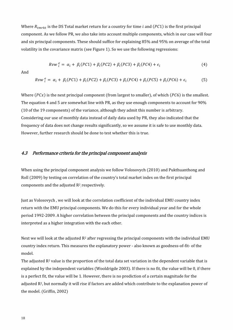
Where is the DS Total market return for a country for time and ( 1) is the first principal
component. As we follow PR, we also take into account multiple components, which in our case will four
and six principal components. These should suffice for explaining 85% and 95% on average of the total
volatility in the covariance matrix (see Figure 1). So we use the following regressions:
+ ( 1) + ( 2) + ( 3) + ( 4) + (4)
And
+ ( 1) + ( 2) + ( 3) + ( 4) + ( 5) + ( 6) + (5)
Where ( ) is the next principal component (from largest to smaller), of which ( 6) is the smallest.
The equation 4 and 5 are somewhat line with PR, as they use enough components to account for 90%
(10 of the 19 components) of the variance, although they admit this number is arbitrary.
Considering our use of monthly data instead of daily data used by PR, they also indicated that the
frequency of data does not change results significantly, so we assume it is safe to use monthly data.
However, further research should be done to test whether this is true.
4.3 Performance criteria for the principal component analysis
When using the principal component analysis we follow Volosovych (2010) and Pukthuanthong and
Roll (2009) by testing on correlation of the country’s total market index on the first principal
components and the adjusted R2, respectively.
Just as Volosovych , we will look at the correlation coefficient of the individual EMU country index
return with the EMU principal components. We do this for every individual year and for the whole
period 1992-2009. A higher correlation between the principal components and the country indices is
interpreted as a higher integration with the each other.
Next we will look at the adjusted R2 after regressing the principal components with the individual EMU
country index return. This measures the explanatory power - also known as goodness-of-fit- of the
model.
The adjusted R2 value is the proportion of the total data set variation in the dependent variable that is
explained by the independent variables (Wooldrigde 2003). If there is no fit, the value will be 0, if there
is a perfect fit, the value will be 1. However, there is no prediction of a certain magnitude for the
adjusted R2, but normally it will rise if factors are added which contribute to the explanation power of
the model. (Griffin, 2002)
19
4.4 The factor models for testing integration
Besides looking for evidence for integration by using the PCA, we will look if factor models are able to
price stocks in the EMU zone. By comparing the factor models using national, EMU and combined
(national and EMU) factors, we can see which country is integrated by testing their explanatory power.
Differences in their explanatory power could indicate which factor is better and should indicate a
degree of integration. If the EMU is completely integrated, there will be no difference in the explanatory
power between the models. As we expect that the EMU is only partly integrated and some countries are
more integrated than others, it is interesting to see how much these factors differ and how much can be
explained by these factors.
Using factor models, we are able to see how much systematic risk is captured by a model, resulting in a
practical way of testing for integration as we are able to see which factor models (national, local or a
combined factor) could be preferable when pricing the stocks.
Using international versions of a factor model to test integration is done by several authors, such as
Jorion & Schwartz (1986), Griffin (2002), Bekaert, Hodrick and Zhang (2005).
4.4.1 The capital asset pricing model
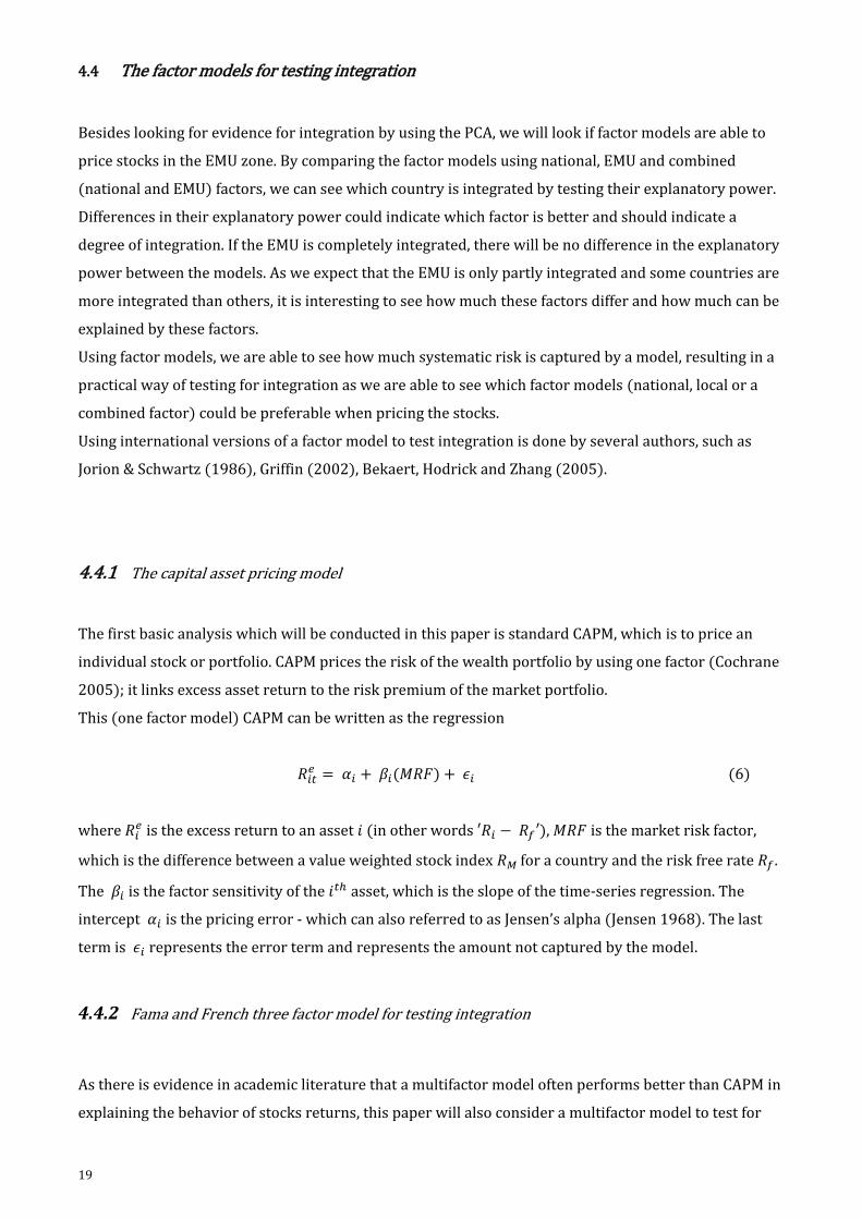
The first basic analysis which will be conducted in this paper is standard CAPM, which is to price an
individual stock or portfolio. CAPM prices the risk of the wealth portfolio by using one factor (Cochrane
2005); it links excess asset return to the risk premium of the market portfolio.
This (one factor model) CAPM can be written as the regression
+ ( ) + (6)
where is the excess return to an asset (in other words ), is the market risk factor,
which is the difference between a value weighted stock index for a country and the risk free rate .
The is the factor sensitivity of the asset, which is the slope of the time-series regression. The
intercept is the pricing error - which can also referred to as Jensen’s alpha (Jensen 1968). The last
term is represents the error term and represents the amount not captured by the model.
4.4.2 Fama and French three factor model for testing integration
As there is evidence in academic literature that a multifactor model often performs better than CAPM in
explaining the behavior of stocks returns, this paper will also consider a multifactor model to test for

20
integration. Therefor this paper will consider the Fama and French three factor model too as a method
for testing integration.
Although there are some articles about using a multi-factor model to test for integration, to this author’s
knowledge only Brooks et al. (2009) use the Fama and French three factor model to test for integration.
Following Fama and French (1992, 1993, 1995, 1996, 1998), we use the extended form of the CAPM, by
adding two extra risk factors.
This will create the Fama and French three factor model (3FM), which contains (1) the market risk
premium, (2) the size factor and (3) book-to-market (or value) factor.
This results the following, which will be tested in this paper
+ ( ) + ( ) + ( ) + (7)
where stands for ‘Small Minus Big’, which is difference in return between a portfolio with small
capitalization stocks and a portfolio containing high capitalization stocks.
stands for ‘High Minus Low’, which is the difference in return between a portfolio with a high
book-to-market stocks and a portfolio containing low book-to-market stocks.
4.4.3 Addition of international factors
Finally, we will take additional EMU factors into account in addition to the local (national) factors in
order to test if local factors have any influence in pricing stocks, as Beale et al. (2004) indicate that
country specific factors are getting less important.
Therefore we create CAPM and the 3FM using only EMU factors:
+ ( ) + (8)
And
+ ( ) + ( ) + ( ) + (9)
Where ( ), ( ) and ( ) stand for the EMU Market risk factor, EMU Size factor and EMU
value factor. We are then able compare the ‘local’ model to the ‘EMU’ model.
Finally, we will create a combined factor model in order to see how much local and EMU factors add:

21
+ ( ) + ( ) + (10)
and
+ ( ) + ( ) + ( )
+ ( ) + ( ) + ( ) + (11)
The local (national) factors ( ), ( ), ( ) are constructed in the same way as the European
factors ( ), ( ), ( ), but only taking national data into account.
By creating these international and combined versions, we can test the influence of national factors in
the pricing model.
This paper will run regressions using the equations (6), (7), (8), (9), (10) and (11) for the 12 Euro zone
countries individually and using equations (8) and (9) for the Euro zone as a whole.
4.5 Performance criteria for the factor model
In order to test the stock pricing ability of the CAPM and the 3FM, we consider two performance criteria
which are the adjusted R2 and the pricing error .
The first performance measure is the adjusted R2, the goodness-of-fit, which is described before (in 4.3).
The second performance measure which will be used is the pricing error , which is the regression
intercept.
It is also known as ‘abnormal’ return, meaning that the stock is able to produce a return which is higher
than the (expected) risk adjusted return. A positive alpha is better for the investor, but it implicates that
the model is less effective. If we take the null hypothesis that the risk factors are responsible for the
generated data, the estimated pricing error should equal to zero. The closer the intercept is to 0, the
better the model is able to price the portfolio as the model appears to more effective.

22
5 Portfolio construction
5.1 Construction of the Fama and French risk factors
In order to construct the factors, this paper will follow Fama and French (1992, 1993) to form six
portfolios with value weighted stock returns. These are constructed from sorting the stocks on their
size and their BEME on an annual base. So the portfolios are rebalanced every year in July.
These portfolios should mimic the size (SMB) and book-to-market (HML) risk factors they represent
(Fama and French, 1993) and provide the explanatory variables for the time-series regression.
Firstly, we rank every stock of the Datastream Total Market on its size on the first of July of year ,
where size stands for the market value of the company, which is price of the stocks times amount of
shares.
Following Griffin (2002), the median (or a percentile of 0.5) is used to divide the stock sample in two
classifications; Small (S) and Big (B). If the amount of stocks is uneven, the median is added to the Small
stock portfolio, which results + 1 stocks in that year.
This is different from Fama and French (1993), as they use the median size of the NYSE , instead of the
complete sample, to divide their sample in a Small and Big portfolio. The consequence of their division
is that the Small portfolio contains more stocks than the Big portfolio, although the market value of the
Big portfolio is still much larger than the Small portfolio. In this paper the Small and Big portfolio
contain the same amount of stocks, but the Big portfolio does have a much larger market value.
This could have consequences for our results, so this should be kept in mind.
Secondly, we break the Small and Big portfolio in three book-to-market groups each. The book-to-
market value is created by the using the book equity of December of 1 divided by the market equity
of December of year 1 (Fama and French, 1993).
The bottom 30% will be classified as Low (L), the middle 40% as Medium (M) and the top 30% as High
(H). As Fama and French indicate, these divisions in classifications are arbitrary.
Using these five classifications (S, B, L, M and H), we will be able to create six portfolios: SL, SM, SH, BL,
BM and BH.
Now we have the ingredients to create the SMB and HML factors.
The SMB (size) factor can be created by taking the difference between average of the small stock
portfolios returns (SL, SM and SH) and the average of the big stock portfolios returns (BL, BM and BH)
for each month. The will look like this:
(SL + SM + SH) (BL + BM + BH)
3

23
The HML (value) factor can be created in a similar way. It is the difference between the average of high
book-to-market equity portfolios returns (SH and BH) and the average of low book-to-market equity
portfolios returns (SL and BL) for every month. This will look like this:
(SH + BH) (SL + BL)
2
For the construction of the portfolio returns we use the value weighted (lognormal) return as described
by Fama and French (1993). The reason for value weighted returns is that we want to minimize the
variance of firm-specific factors. By using value weighted components, the variance is minimized as
return variances are negatively related to size (Fama and French, 1993). Also, it should correspond to
realistic investment opportunities.
This means that the portfolio return is calculated by the following formula:
∑( (
)) (
)
where depicts the return of the portfolio, is the price of stock at moment , while is the
price of stock of month 1. is the market value of company , while is the total market
value of the total market.
In order to create the market risk factor , we use have to calculate the excess return on our value
weighted market portfolio, which is . is created by adding the value weighted returns
minus the value weighted risk-free rate of every stock available in that month together, including the
ones the stocks that were excluded in the portfolio creation (missing data or negative BE-ME values).
5.2 Construction the dependent variables portfolios
For the time-series regression we have to construct nine additional (dependent) portfolios, formed on
size and BEME. For these portfolios, we use the value weighted excess returns of the stocks considered.
This number is smaller than Fama and French (1993), which used 25 portfolios instead of nine.
However, as we have a (very) limited number of stocks in some countries, we are not able to make 25
portfolios.
Except for this difference, we follow them on their methodology in constructing the nine portfolios. The
formation by size and BEME is used in order to see if the SMB and HML portfolios factors capture
common factors in the stock returns which should be related to size and book-to-market stocks (Fama
and French, 1993).

24
Just as we have done for constructing the risk factors, we sort our data by size and BEME. Instead of the
five divisions in the Fama and French factors (two size divisions and three BEME divisions), we make
six division, still using the same criteria.
The divisions for size are made as follows: the bottom 30% will be classified as Small (S1), the middle
40% as Medium (S2) and the top 30% as Big (S3). We have then three size portfolios, which will be
divided again into nine dependent portfolios. Each of the three size portfolios are again evenly divided
into three BEME portfolios: the bottom 30% will be classified as Low (B1), the middle 40% as Medium
(B2) and the top 30% as High (B3).
This results in nine portfolios - Big Size/High BEME value (S3B3), Big Size / Medium BEME (S3B2), Big
Size / Low BEME (S3B1), Medium Size/ High BEME (S2B3), Medium Size/ Medium BEME (S2B2),
Medium Size / Low BEME (S2B1), Small Size/ High BEME (S1B3), Small Size / Medium BEME (S1B2)
and Small Size / Low BEME (S1B1) - which will be used as the dependent variable in the time series
regressions.
Using these nine portfolios the results, such as mean, standard deviation, adjusted R2 etc. – we will be
reported in the tables 1- 13 below.

25
6 Empirical results of factor tests
6.1 Statistics on the factors and portfolios
6.1.1 General statistics
The statistics in Table 1 - 5 show some general information about the data used.
First of all, we compare the constructed market portfolio (Total Market R vw- ‘vw’ means value
weighted) with the Datastream (DS) Total Market Index.
Since we have removed some stocks - due to the lack of currency information, the lack of data for some
stocks in the Datastream (Dead) Stock lists and, even worse, wrongly reported data in Datastream4 - it
is wise to see what the effects are by comparing the two market portfolios. This is done to check the
quality of our own market portfolio compared to the one of Datastream.
Table 1 describes the correlation between the two. The correlations are, except for Luxembourg, all
above the 0.75.
The relatively low correlations in Austria, Belgium, Ireland and the Netherlands could also be partly
explained by the exclusion of some stocks nominated in foreign currencies and the unavailability of
some data for some stocks.
The reason for the low correlation in Luxembourg can be found in the exclusion in quite a number of
stocks that are reported in another currency than the euro, pound sterling, Yen or Dollar. Besides, the
exclusion of one stock in Luxembourg has a major impact as it has a small number of stocks in total.
Still, there is some fear that some ‘static’ stocks are prematurely removed and even worse, Datastream
could have made some errors5.
Secondly, Table 2 shows the number of stocks considered in this paper. Considering the number of
stocks used - which is the almost 21,000 for the EMU zone over the whole period - this is much more
than two papers known to this author about factor models for EMU stock markets, Moerman (2005)
and Hanhardt and Ansotegui (2009), the latter only considers ‘living’ stocks.
Table 2 shows that Germany is clearly the largest and most important economy in the EMU zone, as it
has on average 1370.3 (46% of the EMU zone) stocks in the time period considered. It is also
remarkable that Germany did not have the largest number of stocks in the EMU until 1995. This might
have maybe something to do with the unification of Germany in the former years.
4 It should be noted that the author of this paper found some stocks which were wrongly listed in Datastream ‘Dead Stock list’. In some cases this meant that stocks were listed after their delisting date. But even worse, there are cases in which the price, market value or book value was completely wrong, as the Datastream showed an increase of an exact 1,000 or even 100,000 multiple in the value. Examples are Metro One Dev (Germany) which has a way too high market value and Roche Holdings (France) with a price way too high. In one month time their values are (conveniently) multiplied by 10, 100 or even 1,000. Unfortunately, the number of stocks was too great to check by hand, so these errors could have influenced results. Imagine a company with only 0.01% of the market value being increased to 10%. 5 For example in the Dead stock list in the Netherlands, there is some suspicion that ABN AMRO market value is mixed up, as they show some strange deviations (around the period of the introduction of the euro). Secondly, Datastream gives an error for ABN AMRO, while still stating values.

26
France has the second largest number of stocks, followed by Italy and the Netherlands respectively.
Portugal, Ireland and Luxembourg are the smallest countries, stock wise.
If we mention to the ‘larger EMU countries’, the countries France, Germany, Italy, Spain and the
Netherlands are referred. If we mention ‘smaller EMU countries’, we mean Austria, Belgium, Finland,
Greece, Ireland Luxembourg and Portugal. This division is roughly based on the number of stocks,
although it is still arbitrary, as Belgium has on average a higher number of stocks than Spain.
It is remarkable that most countries have about the same or even less stocks in in the last period (July
2008 until June 2009) compared to the first period (July 1993 until June 1994), except for Germany,
Luxembourg and Spain. Most countries reached the highest number of stocks midway the time period
considered, 1998-2001. This period can be considered as the height of the dot-com bubble. After 2001
in every country there is a steady decline in the number of stocks, probably after the burst of the
bubble. The fluctuations in stocks can be caused by reasons such as bringing stocks to the market,
mergers, acquisitions and bankruptcies.
Thirdly, we look at the number of stocks used per portfolio (the nine Fama and French portfolios) per
country in Table 3. Small numbers of stocks in a portfolio could potentially seriously influence the
results. Except for Luxembourg, every country has have on average more than five stocks in the
dependent portfolios (SxBx). However, five ‘smaller’ countries do have less than 10 stocks in their
portfolio on average. The ‘large’ countries have no trouble in containing a decent number of stocks per
portfolio. Looking at the six factor (S, B, H, M and L) portfolios, only Luxembourg and Portugal have less
than 10 stocks on average in the BH and SL portfolios. These average small numbers of stocks could
result in a small number of stocks in a portfolio in some years, even as little as one.
One should therefore keep in mind that for the ‘small’ countries the explanatory power and reliability of
these portfolios could potentially be biased. A characteristic of a stock in a small stock portfolio could
have a major impact on the portfolio return. Therefore, these portfolio results (and as a consequence
the average results of the country) should interpreted with caution.
6.1.2 Descriptive statistics
Table 4 and 5 describe some general descriptive statistics, which can be compared to other authors and
other countries.
Looking at the skewness and kurtosis, most risk factors show a positive skewness, especially the SMB
risk factor. This means that there is a tendency that these portfolios have a more pronounced right tail,
e.g. there are more returns higher than the mean.
Other way around, the skewness of the HML factors are more evenly divided, but quite a few have a
negative skewness.

27
Looking at the kurtosis, every variable contains a kurtosis higher then 3 - indicating fat tails – with the
highest score under 24.
It is remarkable that the highest kurtosis can be found in the HML factors. This implies that ‘value’
stocks in the EMU zone are sensitive for shocks as they give more ‘extreme’ values. It is hard to say if it
is only smaller countries that have higher kurtosis, as Germany and Ireland are exceptions. An
explanation could be that Germany has a high number of stocks with the same profiles, while Ireland
has stocks which are more evenly divided over several characteristics.
Based on the Jarque-Bera test with 1% significance level we can reject the null hypothesis of normal
distribution in every case, except for two cases. This is an expectation, as realistic financial data are not
normally distributed. This implies that there are more than two parameters (mean return and variance)
to describe the risk-return relation.
This supports our notion that we should use the principal component analysis to test for integration,
instead of the correlation method.
Looking at the mean returns of the factors in Table 4, the market factor (Mrkt-Rf) yield a positive return
although a very small one in Ireland. This is also in line compared with the Datastream Total Market
return (DSMrkt), which is also positive for every country.
The size (SMB) and the value (HML) effect are negative in almost every country. Only Austria, Belgium
and Luxembourg show a positive HML average return in the time period 1993-2009.
This is strange, as it is not in line with Fama and French (1993) and Griffin (2002). This result implies
that if you are long on high book-to-market stocks and short on low book-to-market stock, you have to
pay a premium. So this indicates a reversal of the value effect in the EMU zone. Considering the size
effect, these results indicate that you have to pay a premium if you are long on small capitalization
stocks and short on short big capitalization stocks. This means a reversal of the size effect in the EMU
zone.
It is somewhat similar to a reversal effect described in Faff (2004) and Cochrane (2005). Cochrane
(2005) even states that the factors have declined substantially in recent years, so this could be an
example of the decline of the size and value factor.
6.1.3 Checking the factor results for robustness
As these results are contrary to the results found by other authors and Fama and French themselves,
these results should be checked. These results could cause some suspicion whether or not the
methodology is properly used. As stated in 2.3.4, the Fama and French methodology is not without any
scrutiny. Besides, we do not have any reference points to compare with, as there are no academic
articles written on the 3FM in the EMU zone.

28
Therefore we want to check if the SMB and HML factors will be positive when using a different
methodology.
We have tested several issues: different time samples, a different construction of the dataset and a
different portfolio construction.
Firstly, we have checked if the time sample has any influence on the mean return. Table 5 shows the
results of the 4 different starting periods and a completely different time sample, 1993-2000 instead of
1993-2009.
It is striking to see that when starting the sample in later years, this has a major impact on the average
return, for every year most countries show an increase in (in most cases, a less negative) return.
Most countries have a positive SMB and HML if we consider the time period 2000-2009.
The other way around, the time period 1993-2000 shows negative returns for the factors and in some
cases these negative returns are quite big: e.g. Finland.
This could indicate that the 90’s have had a serious negative impact on the factors.
As the data is checked for exchange risks (all stocks denominated in a foreign currency is properly
converted to the euro), the change to the euro should have no impact.
A possible explanation could be found in the ‘dot-com bubble’, when growth stocks performed better
than value stocks (Baker & Wurgler 2007), as investors wanted to invest in these (IT) stocks. These
stocks increased in value very rapidly, earning a high return and gaining in market value, while small
stocks and low book-to-market stocks were doing mediocre. Another explanation could be that the
growth stocks profited from the bubble, gaining high (or average) positive results, but because of their
high market value they have a larger impact on the portfolios.
This could have resulted in a turnaround in the SMB and HML factors during this period.
Considering the returns of the portfolio and the returns of the SMB factor, it is striking that in almost
every case the monthly SMB return turns out to be positive, only if the ´big´ portfolio return is negative.
This could have several reasons. Firstly, this could be explained by the characteristics of the ´big´ stocks
(see 2.3.3), resulting in the fact that they are more prone to negative sentiments, as they are traded
more often.
Secondly, this can be caused by the construction of the SMB portfolio. The division of the SMB by using
the median can cause the bulk of the market value to be in the ‘big’ portfolio, while only a small amount
of the market value is in the ‘small’ portfolio. This could have an impact on the value weighted returns,
as larger firms achieve a higher (positive or negative) value weighted return.
Changing the construction of the portfolios will be tested later in this paragraph.
Still, other explanations could be possible. We can also look at the construction of the dataset.
As we do take every available stock return and do no limit on a certain appearance threshold, it is
possible that some stocks disappear soon after the creation of the portfolios, resulting in no excess
return.

29
We therefore added some additional limitations in a new dataset: a stock will be removed completely
(not only for the portfolio creation) for the consequent year unless it has a book value in December in
year t-1, a market value of July in year t and it should have a stock price in in July of year t.
Secondly, we added a survivorship bias, by only using stocks which have been listed in two consequent
years, in other words, it should have met the above criteria in July of the year t-2.
However, although this caused a reduction in stocks, especially in the years before 2006 (mostly around
15-25%), it does not cause the SMB and HML factors to improve significantly, they both remain
negative. Again, they start to get positive around the years 1999-2000, although somewhat earlier than
with our original dataset.
We have also run a test using only the ‘living’ stocks, not using the ‘dead stock’ lists, however, this gives
no satisfactory results either.
So, a different dataset construction is not the reason of the negative returns.
Regarding the BEME ratio in the portfolios in Table 6, the results and distributions are comparable to
Fama and French (1993). The only major difference can be found in the BEME H3 portfolios, and
especially the S1H3 BEME portfolio as they are much higher compared to the other BEME portfolios.
These portfolios also have a much higher BEME value compared to the Fama and French’s BEME
portfolio for the United States (their highest BEME value is 1.80 compared to Austria, Greece, Italy and
Luxembourg with 11.05, 10.35, 11.1 and 16.84 respectively).
This indicates these stocks have a very high book-to-market value, much higher compared to the other
portfolios of Fama French, which could indicate that there are in this data set stocks which could be in
distress (a book value which is higher than market value could be a sign of a company going badly).
This could also explain the negative mean return for the value factor, as perhaps some stocks went out
of business. The decreasing number of stocks could support this view.
Even worse, wrong book values or market values could also have contributed to these high values.
In order to test this, we have used several limitations on the BEME ratio, using a limit of 15, 10 and 5 to
see if the results change significantly. However, it does not, as this limit results in the exclusion of only a
minor amount of stocks.
Considering the average size in Table 6, compared to the results of Fama and French (1993), with their
sample of 1963-1991, the difference between S1 (smallest) companies and S3 (largest) companies is
much bigger. This could potentially distort our results, as ‘penny’ – very small stocks- stocks could be
included in the small portfolios.
To correct for this problem, testing indirectly the statements of Kothari et al. (1989), we exclude
smaller stocks. We use several limits, such as € 10mln, 50mln, 100mln, 200mln and 300mln.
This threshold does especially impact the HML factor. By increasing the threshold amount, the HML
increases even to a positive return around the threshold of 200-300mln for the period 1993-2009.
When doing this, though, the average percentage of market value remain under the 10% for most
countries even with the threshold of 300mln although the percentage is much higher in the pre-1997
period and much lower in the post-1999 period.

30
It also has a major impact on the average number of stocks, as countries will lose up to 80% of the
number of stocks with the 300mln threshold. Again, the pre-1997 period will show the sharpest
decrease in the number of stocks.
This means that smaller countries do not have stocks left to form a proper portfolio, so this threshold
should not be considered.
Lastly, we can look at our portfolio construction. A major difference in our portfolio construction is that
we use the median to split our dataset, instead of using the median size of the NYSE which Fama and
French use (see 5.1).
This could cause the negative SMB returns, as we use value weighted returns, meaning that smaller
stocks give a smaller amount of return (as their market value relative to the total market value is small).
All small stocks combined still have a much smaller amount of market value compared to the ‘big’
stocks. So we should look at the ratio of small stocks and big stocks in the SMB portfolio.
Fama and French (1993) indicate that there are a disproportionate number of stocks of 3,616 out of
4,797 in the small stock portfolio in 1991, which is roughly 75%.
So we have started using this division, increasing it with 5% until the moment the factors are positive.
This has a positive impact on the SMB factor, but a negative impact on the HML factor.
When the division is around 85%-90% in the small portfolio, the SMB is getting positive in some
countries, but the HML remains negative.
The high percentage is logical as the most countries have a very big difference between the smallest
portfolio and the largest portfolio. This difference is bigger than Fama and French, so the proportions in
the ‘Small’ and ‘Big’ portfolio should be different.
A test with the creation of the size and value portfolios independent of each other does not give positive
results too.
Ultimately, the best results are achieved when using a combination of a 300mln threshold and 95% in
the small portfolio. The extra limitations of our dataset only results a lowering on the 300mln threshold
to the 250mln threshold (on average), still with 95% in the small stock portfolio.
These conditions mean that a large number of stocks will be removed and that the ‘Big’ portfolio will
only contain a very small amount of stocks. We consider this to be unworkable and it could seriously
bias our results.
This means that our dataset seems to be robust, although the results still deviate from Fama and
French. So we want to stick with our dataset and continue with our research using our data.
Testing with different threshold and conditions has also shown the more stocks from the period 1993-
2000 are removed, the more positive the returns are. It seems that the period 1993-2000 in our dataset
has caused the negative average returns for the SMB and HML factors, which could possibly be
explained by the dot-com crisis. This could support Cochrane’s (2005) statement that the factors are
declining.
31
An extra test could be conducted with another database (instead of Datastream) or only using major
indices. However, this paper will not discuss the values and implications of the factors.
This paper will only look if the factors are able to price the EMU countries and the EMU zone. It is,
however, interesting for further research to look into this phenomenon.
6.2 Results on integration in the EMU using PCA
Considering the question if we find any evidence on integrated EMU stock markets, we started to look at
the first principal component. We use the principal component analysis to produce principal
components (PC), which can be correlated to the country return and can be regressed to produce
adjusted R2.
At first, we look at the trend in the first PC in Table 7 and Figure 1. Here we can check whether stocks
are sensitive to same shocks, e.g. the European factor.
Tests indicated that the PC’s do not correlate with the EMU market factor, EMU HML factor or EMU SMB
factor. So this means that PC’s cannot be identified with one of factors of our model.
We see that the PC increased from 0.45 in 1992 to 0.82 in 2009. This could be interpreted that the
stocks in the EMU zone got more sensitive to the same shock factor. Over the whole period, the value of
the first PC was 0.67, indicating that the first principal component is able to explain two thirds of the
variance in the EMU zone. This is an indication that the EMU has become more integrated over time,
which was to be expected.
Looking at the development of the correlation with the first PC (table 7 and Figure 3), comparing the
correlation in 1992 with the correlation in 2009, we can see that the correlation has increased in every
country. It is remarkable that on average the correlations in the post-2001 are higher than in the pre-
2001 period. This is somewhat to be expected, as the introduction of the euro (as the common
currency) resulted in an extra boost in the integration process.
On average, the major (biggest) EMU countries have the highest correlation with the first PC, while the
smaller countries have a much lower correlation. In line with literature, Greece, Finland and Portugal
(Luxembourg too, but their low number of stocks makes it difficult to interpreted these results), are the
least integrated with scores 0.68, 0.72 and 0.78, respectively. Germany, France and the Netherlands
have the highest correlation, all above 0.90. This was also to be expected as these countries are heavily
externally oriented and were always major players in the European (and world) stock markets.
The economies of these countries are also based on international (European) trade and export, so their
high correlation is no surprise. The smaller countries, such as Portugal and Greece have a strong
tradition of small family run companies. They focus less on trade and export, especially in the pre-euro

32
time period. This means that their stocks are less interesting for investors and are less affected by the
European stock market movements, thus show a lower correlation.
Considering the trend lines in Figure 3, the correlations show a strong upward trend, except for
Luxembourg. Still, looking at the graphs, the lines are not the same in every country. An example for
different trends in the EMU countries is visible in 1993: some sharp increases or decreases compared to
1992 show.
This is also described by Fratscher (2002), who found that there were some low correlations during
this crisis period of 1992-1993 and there was a high degree of integration volatility in the 90’s.
It is also noticeable that Germany, the Netherlands, Spain and France (except for one year), show no
large deviations and a low trend coefficient, compared to the small countries.
This could be an indication that these countries were already quite integrated, while the smaller
countries were not. Therefore the larger countries could be less interesting to use as a way of
diversifying an investment portfolio, resulting in more investments in low correlated (small) EMU
countries after the creation of the EMU. After some time, correlation could have increased because of
the investments made in the smaller countries (Greece, Portugal etc.).
Another consequence of the high integration of the larger EMU countries and the creation of the EMU
zone, is that the cost of equity decreases (see 2.2.2) resulting in the possibilities to invest in riskier
stocks, which can be found in the smaller EMU countries. This again increases the integration process in
smaller EMU countries.
The two years 1999 and 2000 produce the lowest correlations with the first PC, especially in the
smaller EMU countries. This could be possibly explained by the fact that other shocks (explained by
other components) became more important. This could for example be an international event (for
example: the dot-com-bubble, the Asian crisis or Russian crisis) to which every country reacted
differently or it was beyond Europe, which is possibly not captured by the first PC.
Next step is to look at the adjusted R2 in Table 8 to see if the PC factors have any explanatory power.
Looking at the trend in the adjusted R2 with the first PC in the time period considered, it shows the
same trend as the correlations: Larger countries have a higher R2 than smaller countries and there are
higher adjusted R2 ‘s post-2001.
This generally upward trend is in line with literature and not unexpected, as this is the widely believed
trend of European stock markets becoming more integrated. Although the period is too short (and the
frequency of data is only monthly) to conclude the integration is substantial, the integration is apparent.
It is remarkable that Austria, Greece, Luxembourg and Portugal even have some negative adjusted R2 ‘s.
Again, we see that there is no parallel increase in the adjusted R2. The only major parallel in every EMU
country which can be found is the dip in 1999-2000. Finland, Greece and Luxembourg have the lowest

33
adjusted R2, having scores between 0.52, 0.47 and 0.46 respectively. In Germany, France, Netherlands
with adjusted R2 of 0.86, 0.84 and 0.87, the first PC has the most explanatory power.
If we add extra principal components (Table 9 and 10), so more shocks are accounted for, the
explanatory power jumps to 0.70 or more. So there are 4 types of shocks in the EMU zone that can
explain more than 70% of the return, with 6 types of shocks by which more than 78% (for some even
more the 90%) can be explained. It is remarkable that Luxembourg jumps to the highest adjusted R2. So
one of the three important other components which explain the returns in the EMU, is much more
important for Luxembourg than for other EMU countries. However, it should be remembered that a fair
number of stocks in Luxembourg are denoted in non-euro currencies.
Based on these results, we see evidence of (growing) integration in the EMU stock markets. However,
there are differences in integration.
One could conclude that the larger countries are more sensitive to the same shock due to higher
integration with each other. In line with Yang, Min and Li (2002), we find evidence that smaller
countries are less integrated, so less sensitive to the same factors – the EMU.
Implications of the initial low correlations of the smaller EMU countries with the first PC is that they
could be used as a way of diversification, however, as the EMU has become more integrated, these
benefits faded away.
The increased integration of the financial market could also strengthen the economies of the smaller
countries as the larger integrated EMU countries will invest more in them.
In the end this means that international diversification through EMU countries is getting less attractive
for investors. Investors should look for other means of diversification to achieve diversification benefits,
such as industry diversification or non-EMU country diversification.
As we have found evidence for integration, we go to the next step, by looking if risk factors are able to
price the return in the EMU countries.
6.3 Results on the risk factors
6.3.1 The ability of the local CAPM and the 3FM to price stocks
In this section we will look into the question which factor model is best at pricing the EMU zone and
how good a local model is compared to an EMU model, using the performance measures R2 and α.
Firstly we look which model is better at pricing the stocks for the EMU countries. Table 11 shows the
average results for CAPM and the 3FM per country.
In these results we can see clear evidence that the 3FM is performing better in the adjusted R2. While
the average adjusted R2 for the local CAPM ranges from 0.151 for Luxembourg and 0.258 for Germany,

34
to 0.526 for France and 0.646 for Italy, the local 3FM ranges from 0.280 for Luxembourg and 0.453 for
Portugal to 0.711 for Italy and 0.652 for the Netherlands. This means that by adding other risk factors
SMB and HML, the explanatory power increases. Looking at the adjusted R2 of the EMU factors and the
combined factors, we see the same tendency: higher scores for the 3FM.
If we look at the nine portfolios individually, we see the same thing, indicating that for every portfolio
the explanatory power increases by adding the additional size and value factor.
Another tendency we see is that countries with a high number of stocks in the dataset have a higher R2,
although when using the 3FM countries such as Austria and Finland show a remarkable leap in the
explanatory power. This is possibly explained by the number of small companies is these countries.
The case for Germany is less clear, as the explanatory power of the local models is lagging compared to
the rest. This has probably has to do with high amount of stocks, of which most are small compared to
the rest of the EMU zone (see Table 6).
Although this looks promising for the 3FM, looking at the pricing errors α, the tendency is less clear.
Except for Belgium and Ireland, the local 3FM produces a higher (or as the pricing error is often
negative, a more negative) pricing error for the local CAPM. In some cases the pricing error even
doubles compared to the local CAPM.
Overall the 3FM possess more explanatory power then CAPM, based on the adjusted R2. However, this is
somewhat offset by a worse pricing errors.
This is line with other authors such as Bekaert, Hodrick and Zhang (2005), who find evidence that the
3FM is better at pricing the stocks than CAPM (using only the adjusted R2).
However, when considering the 3FM, the S3H3 and (in lesser degree) S1H1, it delivers much better R2
’s, which do not look awkward anymore. Apparently, the SMB and HML add much to the explanatory
power when considering these extreme portfolios.
Even if we do take these two portfolios into account, it is clear that the S3 portfolios have the highest
adjusted R2 in every model, but also the highest pricing error. The S2 portfolio follows, while the S1
portfolios produce the lowest adjusted R2. From these results we can conclude that the factor models
are better able to explain larger companies than smaller companies.
However, picking S1 portfolios often delivers an abnormal (although low) return, contrary to the S3
portfolios which often provide a negative alpha.
Looking at the H-portfolios, it is unclear which portfolios produce the highest adjusted R2 and lowest
pricing error on a structural basis.

35
6.3.2 Measuring integration in the EMU zone
The next step is whether there is evidence that EMU factors are also able to explain local returns in the
portfolios. This could be evidence of financial integration. We test this by using EMU factors instead of
local factors and adding the EMU factor to the local models.
Looking at the results of using only the EMU factors instead of the local factors, it is striking to see that
for the CAPM model every small country sees a sharp decrease in R2, while every large country sees
only a small decrease or even an increase in the explanatory power.
However, again, we see an increase in the pricing error for the large countries. This is an indication that
the larger countries are better integrated in the EMU. This in line with what we found earlier, meaning
that the bigger (better integrated) countries are able to be priced with one EMU factor instead of a
national factor for each country.
Looking at the 3FM, we see the same tendency, small countries show a large decrease in the R2, while
the larger countries only display a limited decrease or increase (France). Then again, it is remarkable
that Spain, Italy and the Netherlands show a major decrease in their R2.
If we take the pricing errors for the EMU factors, the 3FM performs fairly well, pricing error-wise. Here
it produces (mostly slightly) lower pricing errors, except for France, Germany and Netherlands, three
large countries. So here it is the other way around, countries with a low number of stocks, produce a
lower pricing error. Portugal is an exception to this tendency, although the pricing error itself is low
compared to the three large countries.
On the other hand, smaller countries see a decrease in pricing error when using the EMU factors for the
3FM.
Comparing the decrease from the local CAPM and 3FM to the EMU CAPM and the EMU 3FM, show that
the decrease in the EMU CAPM is smaller than the decrease in EMU CAPM in most countries. This
indicates that the EMU Market return is gaining importance.
It is remarkable that especially the medium sized portfolios (S2) show an increase in explanatory
power when using the EMU factor. This could indicate that they are getting more dependent on the EMU
market.
On the other hand, it seems that the EMU SMB and EMU HML are less appropriate for these countries,
adding little to the EMU CAPM compared to the local CAPM. Apparently HML and SMB factors are local
and differ from factor loading from each other.
Using the local and EMU 3FM increases the R2 in every country and decreases the pricing error
compared to the local 3FM. Here we find evidence that the combined 3FM is the best model in pricing
stocks. However, the increase in explanatory power in local factors to the combined factors is not very
large in most countries. Belgium and France show the largest increase, while Germany and Portugal
show the smallest. Although this is an indication that EMU stock markets do depend on each other, local
factors are still dominant in the time period considered.

36
It is, however, somewhat striking to see that Germany has one of the lower R2 and the lowest increase
going from local to the combined model. This could be explained that Germany is the largest EMU
member and is in itself very dominant in the EMU. It is more influenced by outside factors in the world
than in the EMU itself, as it is an exporting country to the rest of the world. Countries such as Belgium,
France and the Netherlands have a high exposure to other EMU countries resulting in a high adjusted
R2. Portugal, Ireland and Finland (and Luxembourg) have the lowest adjusted R2 in the EMU zone.
Probably because they are small and the least integrated in the EMU.
Comparing the local and EMU portfolios, it is striking to see the difference between large (S3) and small
(S1) portfolios for every country look at the local CAPM. However, if we consider the EMU factors, there
is a much less pronounced difference.
Considering the 3FM, the differences between the large and small portfolios are much bigger for the
local portfolios. When comparing these results to the EMU 3FM it is remarkable that the difference is
much less pronounced.
Although the differences, this indicates that larger companies can be somewhat more explained by EMU
factors, especially with the EMU market return, which could be an indication that they are more
integrated in the EMU market than smaller ones. This this can be explained that larger companies often
have more international operations.
However, apparently the EMU SMB and EMU HML factors have much less additional explanatory power
compared to the local SMB and HML factors. This is especially true for the large (S3) portfolios, adding
these factors to the EMU CAPM do not increase the explanatory power much.
This could indicate that the SMB and HML factors differ in the EMU countries from each other, while the
EMU market return is more pronounced. The EMU market return is apparently an important
explanatory factor.
All together, we see evidence that the EMU zone integrated – to a certain degree. However, the addition
of EMU factors to the local factors is not that significant. This could have several reasons; one reason
could be that although the EMU is integrated, the characteristics of the EMU stock markets are still very
different. In one country small stocks are very dominant, while in another it is not. Possibly the
characteristics of these stock markets were different before the introduction of the euro and got more
similar after the euro became the common currency.
It is therefore interesting to see whether this has increased over time or if it was already high since
1993 and if there is a difference in the period before and after the euro.
6.3.3 The factor models in the EMU over time

37
To do so, we have divided the data sample in two, conveniently pre-2001 and post 2001. We do expect
an increased integration, as this is the year when the euro was introduced as the common currency and
all ‘old’ domestic currencies could not be used anymore. The question is how much better the EMU
factor in the post-2001 period.
We can see in Table 14 a tendency that the explanatory power of the CAPM with EMU factors has nearly
doubled or even more for every country, except for Belgium, Germany, France, Netherlands and Spain,
which show an increase, but not as drastic as the rest. These countries are expected to be already
somewhat more integrated with the EMU. Still, the pricing errors have increased, except for the small
countries.
When looking at the combined (local and EMU) 3FM, we see that the adjusted R2 has increased
everywhere and the pricing error has decreased in most of the cases. It is interesting to see that the
increase from adding the local factors to the EMU CAPM added more explanatory power in the pre-2001
period then in the post-2001 period. This is still a strong indication that the EMU got more integrated
after 2001, which was expected. The effect of the local factor has decreased after 2001.
Looking at the pricing errors, there is no clear trend for the CAPM models.
Looking at the EMU 3FN and the combined 3FM, we see the same development.
The explanatory power of the 3F models is much higher in the post 2001 period, especially for the
combined factors, where the pricing errors are also lower.
An exception is Finland, which is the only country where the adjusted R2 decreases somewhat in the
post-2001 period.
Considering the addition of local factor in the two periods, they add to the adjusted R2 in the post-2001
period, but less compared to the pre-2001 period. The exceptions are the larger countries France,
Germany, Italy and the Netherlands where adding the local factor in the post-2001 even decreased the
adjusted R2 . This probably has something to do with the difference in local and EMU SMB and HML
factors. An explanation could be that as these countries are very integrated within the EMU, their small
size and values tocks are very much depended on EMU shocks, not so much on local shocks any more.
It should also be noticed that adding the local factor decreases the pricing error in every country except
for Germany. This means that by adding local factors in the post-2001 period, the explanatory power
decreases at every aspect. This should not be a surprise as the Germany is the largest stock market in
the EMU and very much depend on its international trade.
When it concerns the results, the overall picture is that there is a tendency that smaller countries
became more integrated after 2001. The addition of a local factor has less impact in the post-2001
period than before.
On the other hand, the larger countries (especially France and Germany) had already a higher degree of
integration and the differences between the pre- and post-2001 period is limited. Also the addition of
the local factor for these two countries is limited. Spain and Italy, two other large countries, are heavily
38
affected by adding the local factor in the pre-2001 period, while in the post-2001 period the impact is
very limited. Italy has even the highest scores for the CAPM and 3FM models using the EMU factors,
meaning stock index is gotten highly integrated after 2001.
This is in line with Baele et al. (2004) who expected that local factors are getting less important.
Again the implications of integration are apparent, as the larger countries were already integrated,
meaning that investors looked for diversification benefits in other less integrated EMU countries. This
could have resulted in the increase of integration (and decrease the importance of local factors) in the
post-2001 period.
6.3.4 Pricing the EMU zone as a whole
Finally, we want to see what happens if we use the EMU factors only to explain the returns in the whole
of the EMU. It appears (using Table 14) that an EMU CAPM and an EMU 3FM is fairly capable of pricing
the stocks in the portfolios with an adjusted R2 of 0.584 and 0.707 respectively.
These are on average much higher scores (except for the France EMU 3FM) when using the an EMU
model to price the EMU as a whole than using the EMU factors to price the countries individually. Even
the pricing error is lower for most countries.
If we look at the portfolios individually in Table 12 (continued) and Table 13 (continued), it is
remarkable that the almost all adjusted R2’s are higher for portfolios than scores for individual country
produced by the EMU factors, except the S1H1 portfolios. The S1H1 seems to produce a lower score in
many countries. This could be explained that other factors are much more important for these small
companies, such as local factors, as many small companies are not that well integrated in the EMU.
Oppositely, it seems that larger companies are much more integrated as they are well explained by EMU
factors. This could be causes by better international integration, as larger companies often have
international operations or are big enough to be influenced by international (EMU) factors.
Still, it is interesting to see how much the ‘S’ portfolios have lower scores in some cases.
Ultimately, if we consider the combined factor models compared to the EMU factors alone, the EMU
factors show a higher or comparable adjusted R2 for most countries. Even looking at the pricing errors,
while the EMU CAPM shows higher pricing errors, the EMU 3FM shows smaller pricing errors in most
cases.
It seems to be that factors models are able to price all EMU stocks combined fairly well. Looking at the
development of the EMU models pre- and post-2001, again we see that the EMU has become more
integrated, event to the point that EMU stocks can be pooled together and priced by EMU factors.
This could lead to the conclusion that in the current state of the EMU, integration is at a level that we
could pool all stocks from the EMU markets together and then we are able price them better than taking

39
every EMU country individually. This would be ultimate form of integration as we do not have to create
separate factor models for different countries, but we could use only one model.

40
7 Conclusion
In this paper we have tried to provide an insight in the integration of the stock markets in the EMU zone
and examine different factor models to see which is better at pricing the stocks in the EMU zone.
Currently there are a few studies on whether or not the EMU zone should be regarded as one integrated
stock market and what this means for pricing stocks. This is an interesting question as a completely
integrated EMU market could have a major impact on the way how we price assets in Europe and how
achieve a well-diversified portfolio.
However, there still is little recent academic literature on EMU stock market integration and on the way
we price EMU stocks.
This paper’s main contribution is providing evidence of EMU stock market integration by using a non-
correlation method and asset pricing models, and what asset pricing model is able to price the stocks
best in the integrated EMU zone.
Although we expect the EMU market fairly integrated, we wanted to test this assumption. If we find
evidence for this assumption, then it is interesting to know if the stocks could be priced by the same risk
factors, which could indicate if the market is really integrated. Do national risk factors still add
something to the pricing of EMU stocks? Or is one EMU risk factor able to price all EMU stocks?
To examine if the risk factors in the EMU zone are able to price stocks, we use the CAPM and Fama and
French three factor model. This means that we want to test if the market factor, the size factor and
book-to-market factor are common risk factors.
Firstly, we have looked (a) if there is evidence for 12 initial EMU countries stock market to be
integrated in the time period 1992-2009 (monthly data).
We have followed Volosovych (2010) and Pukthuanthong and Roll (2009) in their use of the principal
component analysis in order to see if the stock markets in the EMU zone are correlated with the first
principal component. We used the correlation coefficient and the trend in the coefficients to test this.
By doing this, we see that there is an increasing trend in the correlation.
After doing this, we have regressed the EMU country’s total market index with the first, the first four
and the first six principal components to see how much is explained by the adjusted R2.
By doing this we find evidence that there is indeed increasing integration in the EMU zone. Although
larger countries were already more integrated and show a high degree of integration compared to the
smaller countries, the small countries are getting more integrated and show a higher increase in
integration, especially after 2001.
This has implications for investors as their diversification opportunities within the EMU will decline. If
we follow Goetzmann et al. (2005) we could even say that in the post-2001 period, as integration is high
in the EMU zone, EMU stock markets could be interpreted as bearish.
41
Secondly, we have constructed the CAPM and the Fama and French three factor model (3FM) for the 12
EMU countries and for the EMU zone as a whole. Following Fama and French (1993) and Bekaert,
Hodrick and Zhang (2005) we have constructed local, EMU and combined factor models to see which
one is best as pricing stocks.
We have shown that based on the adjusted R2 and the pricing error α (b) the 3FM is better at pricing
EMU stocks then the CAPM in all cases. This is line with existing literature, which also show that the
3FM is better at pricing stocks than CAPM. This strengthens the 3FM case as this papers uses the EMU
zone as test area, for which academic literature is very limited.
Looking at the EMU factors compared to the local factors (c) they are able to price the stocks of the EMU
zone, but the adjusted R2 is lower for all factor models.
When using EMU factors for CAPM, there is a decrease, but the decrease is relatively small. This
indicates that the EMU market return is getting important. Especially the medium (S2) portfolios show
an increase in many countries, indicating that medium sized companies are getting more integrated
with the EMU.
In the case of the 3FM, using the EMU factors produce somewhat lower pricing errors compared to
using local factors. We see that the larger countries (e.g. France, Germany and the Netherlands) show
little decrease or even some increase in the R2 when using the EMU CAPM instead of local factors,
indicating that they are more integrated in the EMU zone. This could be expected as these countries are
internationally focused. Smaller countries on the other hand, show a large decrease in R2.
The addition of the EMU SMB and HML factors for the countries individually results in a worse
performance, as the decline in explanatory power is larger for the 3FM than compared to the CAPM.
This could indicate that the SMB and HML are not similar in the EMU zone and do not add that much for
smaller countries compared to the local SMB and HML.
When we use the combined factor models (local and EMU factors) we see that (d) the addition
produces little extra explanatory power to the adjusted R2 for CAPM and the 3FM. Still, the combined
factor models produce the highest adjusted R2’s. The combined 3FM also produces the smallest pricing
errors, making it the best model so far.
Again there is a difference between larger and smaller countries, as the differences in the larger
countries between the local, EMU and combined factors are smaller. This indicates that these factors are
more similar and so, these countries are more integrated.
These results could be somewhat biased because of the lack of integration in the first half of our data set
(pre-euro). So the next step we took was to look to split the data set into two periods, pre-2001 and
post-2001, and see if there are differences in explanatory power in the models.
We find that (e) there is an interesting tendency that the local factors added more to the explanatory
power in the pre-2001 period than in the post-2001 period. In other words, the local factor is becoming
42
less important in the recent period. This can be seen in the difference between the models using only
the EMU factors and the models using the combined factors. This is especially true for smaller countries,
seeing the adjusted R2 increase drastically when adding the local factor in the pre-2001 period, while
this effect is fairly limited in the post-2001 period. The EMU zone got more integrated after 2001 and
the local factors are getting less important, which is in line with Baele et al. (2004).
This is in line with the first PC tests, which show a larger increase in the degree of correlation for the
smaller countries.
Finally, we find evidence that (f) EMU factors are able to price the EMU zone as a whole.
If all the stocks are pooled together in one EMU stock market, an EMU CAPM and EMU 3FM is able to
price the whole zone much better than the countries individually. Even compared to a combined factor
model pricing, an individual EMU country often produces a higher adjusted R2 and a lower pricing
error.
If we look at the local portfolios, it is striking to see the difference between large (S3) and small (S1)
portfolios for every country. However, if we consider the EMU factors, there is a much less pronounced
difference. Although the difference is smaller, this indicates that larger companies can be somewhat
more explained by EMU factors, which could be an indication that they are more integrated in the EMU
than smaller ones. This this can be explained that larger companies often have more international
operations.
In many cases the EMU market factor (thus EMU CAPM) has more explanatory power than the local
versions, indicating that the EMU market factor is getting more important. It is, however, interesting to
see that the EMU SMB and HML factor add much less to the EMU CAPM than the local versions.
In the end, it shows that the common EMU factors are able to price EMU stocks very well.
This paper has provided recent support that the EMU is getting more integrated, although larger
countries were already integrated. The largest increase in integration is found for the small countries.
Secondly, this paper has provided empirical support for the 3FM being to explain return better than the
CAPM.
Finally, it provides evidence that EMU factors are getting more and more important and the EMU factor
is even capable of pricing the EMU zone as a whole. Although this is especially true for the large
countries, EMU factors are not able to explain the returns of the small countries very well.
7.1 Further research
While writing this paper, several interesting areas showed up which require some more research and
could add more insights, and possibly some more robustness, for the results showed here.

43
Firstly, it could be interesting check for other integration consequences. It could be interesting if there
is a division in the integration within the EMU countries, like a north-south division. France, for
example, could be more integrated with other southern European countries.
On the other hand, as country diversification is less interesting, it could be interesting to check for the
integration within the EMU industries. Are these industries also more integrated or are only some
industries integrated?
Secondly, one might want to check the data and do the same test with another database, such as the
MSCI, not only for the PCA, but also for the factor model tests.
As stated before, the data produced by Datastream reveals some uncertainties, especially for the
country’s ‘Dead stock list’. If there is a database which shows the complete constituency list per year, it
would be easier to produce results and maybe more accurate. Especially because some authors, such as
Faff (2004), pointed out that the data selection could potentially bias results.
Another test one might want to consider is using only major stock markets indices. Although this could
potentially limit the number of stocks, it could more usable for investors. Often small stocks are hard to
find or track, so they are not used in the ‘real’ portfolio forming anyway. Besides, information for these
stocks is less sensitive for errors.
Finally, it is interesting to test the methodology of the Fama and French three factors for the EMU zone.
What, if at all, and how big are the factors in Europe exactly? This paper only touched this subject only
briefly and there are no academic reference points.
It would be interesting to conduct a thorough methodological test to see if there still is a size a value
effect. This paper finds some evidence which might support the claim that there is possibly a reversal in
the size and value factors. This could be the result of the used methodology used or wrong database in
this paper, but may be the Fama and French factors have truly changed.
One might want to consider different portfolio constructions. Even Fama and French (1993) admit it,
the current splits in the construction is arbitrary. Especially if one wants to look at individual (small)
countries, such as Portugal and Ireland. These countries produce portfolios containing a very limited
number of stocks, which could potentially produce in biased results. Different split strategies could
produce more even divided portfolios.
Even the annual formation now widely used in academic research on the Fama and French could be
outdated. If we look at the current actual used portfolios (take IShares or MSCI), these portfolios are
rebalanced quarterly or even monthly.
When Fama and French conducted their research in 1993, they used data ranging from 1963 until 1991.
Even their more recent papers (and others) date from the 1990’s. These were the times that computers
were almost non-existent, most brokers were still working on the exchange floor and internet was
(almost) nonexistent.

44
The development of computers and internet made it possible trade stocks quickly, access all sorts of
information and calculate sophisticated portfolios. Investors were also able to utilize certain anomalies
quickly, making them possibly disappear, while other anomalies were able to come into existence.
Now looking at the MSCI for example, they have publicly traded ‘size’ and ‘value’ indices, which could
have potentially reduced the anomalies.
Thus, is could be very relevant to reinvestigate the methodology of the Fama and French three model, as
times has changed, possibly changing the risk factors too.
As these questions indicate, there still is a lot to research in the area of the CAPM and the 3FM.
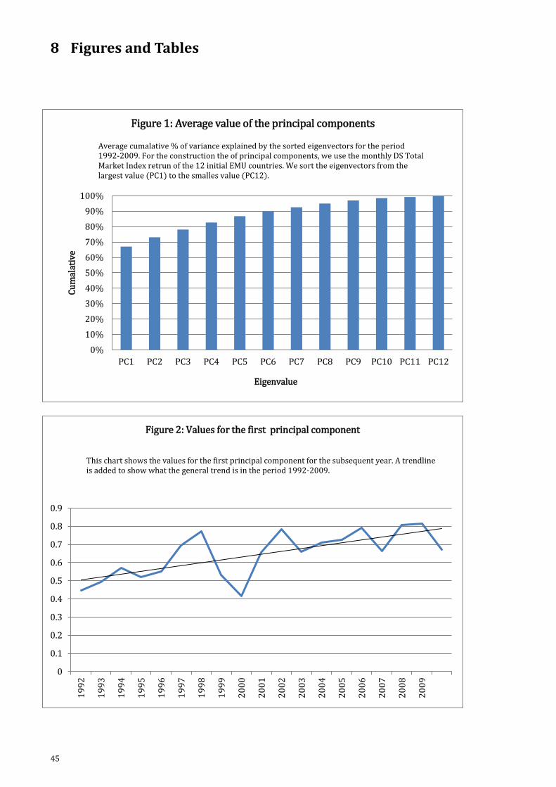
45
8 Figures and Tables
0%
10%
20%
30%
40%
50%
60%
70%
80%
90%
100%
PC1 PC2 PC3 PC4 PC5 PC6 PC7 PC8 PC9 PC10 PC11 PC12
Cu
mal
ativ
e
Eigenvalue
Figure 1: Average value of the principal components
Average cumalative % of variance explained by the sorted eigenvectors for the period 1992-2009. For the construction the of principal components, we use the monthly DS Total Market Index retrun of the 12 initial EMU countries. We sort the eigenvectors from the largest value (PC1) to the smalles value (PC12).
0
0.1
0.2
0.3
0.4
0.5
0.6
0.7
0.8
0.9
19
92
19
93
19
94
19
95
19
96
19
97
19
98
19
99
20
00
20
01
20
02
20
03
20
04
20
05
20
06
20
07
20
08
20
09
Figure 2: Values for the first principal component
This chart shows the values for the first principal component for the subsequent year. A trendline is added to show what the general trend is in the period 1992-2009.

46
Tab
le 1
: Co
rrel
atio
ns
bet
wee
n T
ota
l Mar
ket
R v
w (
val
ue
wei
ghte
d)
and
DS
(Dat
astr
eam
) T
ota
l mar
ket
In
dex
EM
U
DS
To
tal
Mar
ket
R
Spai
n
DS
To
tal
Mar
ket
R
0.9
66
8
Po
rtu
gal
DS
To
tal
Mar
ket
R
0.9
88
9
Net
her
lan
ds
DS
To
tal
Mar
ket
R
0.7
64
7
Lu
xem
bo
urg
DS
To
tal
Mar
ket
R
0.5
71
5
Ital
y
DS
To
tal
Mar
ket
R
0.9
92
5
Irel
and
DS
To
tal
Mar
ket
R
0.7
99
6
Gre
ece
DS
To
tal
Mar
ket
R
0.9
88
1
Ger
man
y
DS
To
tal
Mar
ket
R
0.8
30
2
Fra
nce
DS
To
tal
Mar
ket
R
0.9
18
3
Fin
lan
d
DS
To
tal
Mar
ket
R
0.9
97
0
Bel
giu
m
DS
To
tal
Mar
ket
R
0.7
88
2
Au
stri
a
DS
To
tal
Mar
ket
R
0.7
51
9
To
tal
Mar
ket
R
vw

47
A
ver
age
72
.9
14
1.1
7
1.8
4
99
.6
13
70
.3
10
6.9
5
7.7
2
17
.3
33
.4
19
7.3
6
4
12
8.5
2
96
0.7
Tab
le 2
: Nu
mb
er o
f st
ock
s u
sed
fo
r p
ort
foli
os.
Per
iod
fro
m J
uly
19
93
un
til J
un
e 2
00
9
20
08
50
1
05
5
6
30
0
83
1
64
5
3
18
2
25
1
52
4
5
12
4
19
87
20
07
49
1
03
6
3
32
8
14
49
7
1
55
1
83
2
8
16
2
46
1
23
2
66
0
20
06
48
1
14
6
5
34
7
18
27
8
1
48
1
89
3
2
16
6
52
1
20
3
08
9
20
05
53
1
15
6
8
37
2
21
11
9
6
49
1
93
3
5
17
3
51
1
27
3
44
3
20
04
56
1
22
7
2
42
2
22
37
1
10
5
0
19
2
35
1
83
5
4
12
5
36
58
20
03
68
1
30
7
4
47
2
23
31
1
20
5
4
21
1
36
1
95
5
8
13
7
38
86
20
02
77
1
41
8
1
54
6
24
59
1
41
6
2
22
8
40
2
02
6
2
14
6
41
85
20
01
84
1
56
8
7
58
2
24
96
1
48
6
6
23
3
44
2
46
7
2
14
6
43
60
20
00
84
1
61
9
0
59
3
15
28
1
38
7
1
22
8
48
2
71
7
6
14
3
34
31
19
99
10
6
15
4
90
6
24
1
03
4
12
3
71
2
17
4
6
27
7
84
1
43
2
96
9
19
98
93
1
60
8
5
63
1
83
1
12
6
65
2
22
4
8
25
9
95
1
37
2
75
2
19
97
94
1
62
7
6
61
1
70
5
12
6
58
2
30
3
0
21
8
91
1
28
2
52
9
19
96
80
1
54
6
9
52
7
56
4
10
2
55
2
26
2
5
16
9
65
1
19
2
15
5
19
95
80
1
57
6
4
54
1
53
0
96
5
5
23
4
24
1
69
6
0
11
4
21
24
19
94
76
1
64
5
4
54
6
50
9
86
5
6
25
1
19
1
60
5
9
11
2
20
92
19
93
68
1
60
5
5
55
1
48
3
82
5
5
25
8
19
1
54
5
4
11
2
20
51
Au
stri
a
Bel
giu
m
Fin
lan
d
Fra
nce
Ger
man
y
Gre
ece
Irel
and
Ital
y
Lu
xem
bo
urg
Net
her
lan
ds
Po
rtu
gal
Spai
n
EM
U z
on
e (t
ota
l)
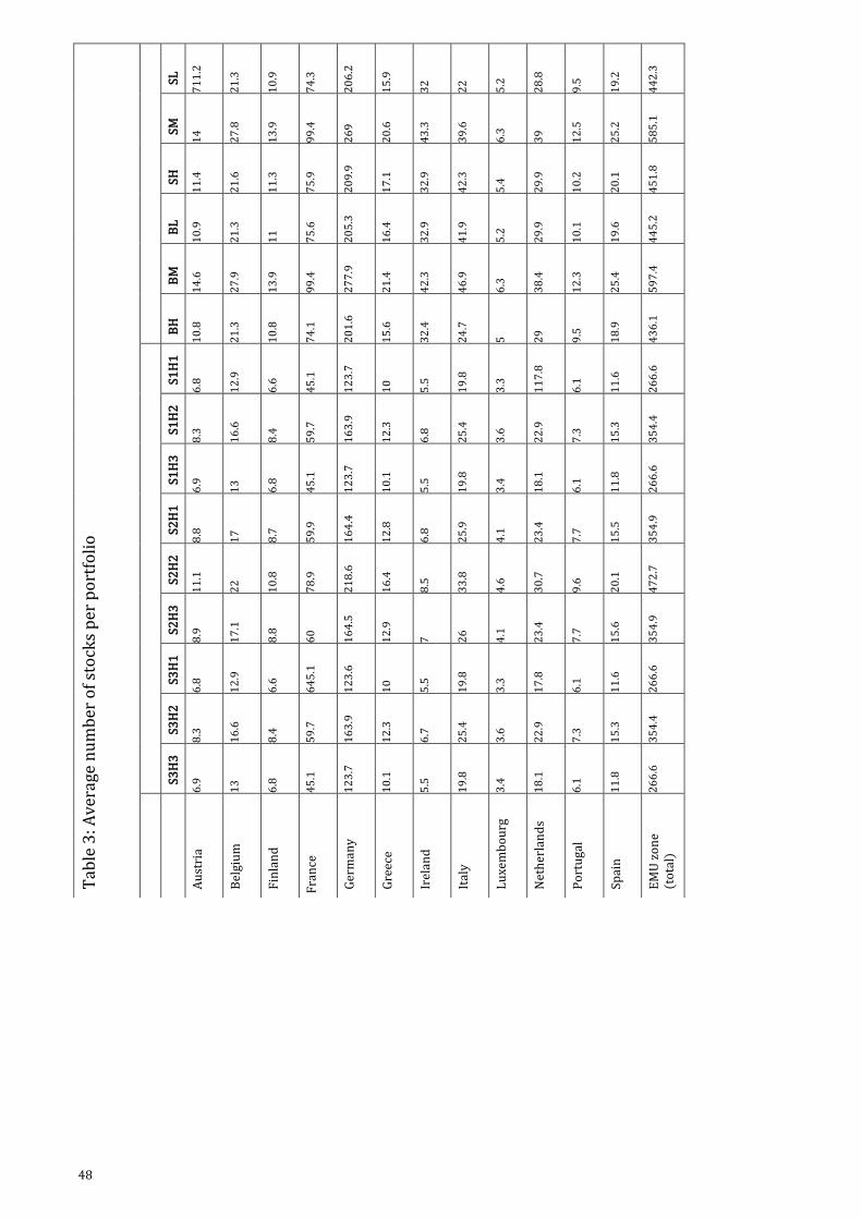
48
T
able
3: A
vera
ge n
um
ber
of
sto
cks
per
po
rtfo
lio
SL
71
1.2
21
.3
10
.9
74
.3
20
6.2
15
.9
32
22
5
.2
28
.8
9.5
19
.2
44
2.3
SM
14
27
.8
13
.9
99
.4
26
9
20
.6
43
.3
39
.6
6.3
39
1
2.5
25
.2
58
5.1
SH
11
.4
21
.6
11
.3
75
.9
20
9.9
17
.1
32
.9
42
.3
5.4
29
.9
10
.2
20
.1
45
1.8
BL
10
.9
21
.3
11
75
.6
20
5.3
16
.4
32
.9
41
.9
5.2
29
.9
10
.1
19
.6
44
5.2
BM
14
.6
27
.9
13
.9
99
.4
27
7.9
21
.4
42
.3
46
.9
6.3
38
.4
12
.3
25
.4
59
7.4
BH
10
.8
21
.3
10
.8
74
.1
20
1.6
15
.6
32
.4
24
.7
5
29
9.5
18
.9
43
6.1
S1H
1
6.8
12
.9
6.6
45
.1
12
3.7
10
5.5
19
.8
3.3
11
7.8
6.1
11
.6
26
6.6
S1H
2
8.3
16
.6
8.4
59
.7
16
3.9
12
.3
6.8
25
.4
3.6
22
.9
7.3
15
.3
35
4.4
S1H
3
6.9
13
6.8
45
.1
12
3.7
1
0.1
5.5
19
.8
3.4
18
.1
6.1
11
.8
26
6.6
S2H
1
8.8
17
8.7
59
.9
16
4.4
12
.8
6.8
25
.9
4.1
2
3.4
7.7
15
.5
35
4.9
S2H
2
11
.1
22
10
.8
78
.9
21
8.6
16
.4
8.5
33
.8
4.6
30
.7
9.6
20
.1
47
2.7
S2H
3
8.9
17
.1
8.8
6
0
16
4.5
12
.9
7
26
4.1
23
.4
7.7
15
.6
35
4.9
S3H
1
6.8
12
.9
6.6
6
45
.1
12
3.6
10
5.5
19
.8
3.3
17
.8
6.1
11
.6
26
6.6
S3H
2
8.3
16
.6
8.4
59
.7
16
3.9
12
.3
6.7
25
.4
3.6
22
.9
7.3
15
.3
35
4.4
S3H
3
6.9
13
6.8
45
.1
12
3.7
10
.1
5.5
19
.8
3.4
18
.1
6.1
11
.8
26
6.6
Au
stri
a
Bel
giu
m
Fin
lan
d
Fra
nce
Ger
man
y
Gre
ece
Irel
and
Ital
y
Lu
xem
bo
urg
Net
her
lan
ds
Po
rtu
gal
Spai
n
EM
U z
on
e (t
ota
l)

49
Table 4: Summary Statistics for the factors and the DS Market Indices, full sample period
Annualized summary statistics for all risk factors in the considered countries in the EMU zone and the EMU zone as a whole. The factors Mrkt-RF, HML and SMB are constructed from all available stocks from Datastream. Mrkt-RF is the return to the market risk factor (value weighted market return minus the risk free), HML is return on a portfolio which is long on high book to-market stocks and short on low-book-to-market stocks and SMB is the return on the portfolio which is long on small capitalization stocks and long on big capitalization stocks. DSmrkt is the total market return index from Datastream. *, **,*** are used to indicate the significance level - at 10%, 5% and 1% respectively - for the Jarque-Bera test.
Mean Std. Dev. Skewness Kurtosis Jarque-Bera Austria Mrkt-Rf .0218 .7586 -.5488 5.5229 60.56*** HML .0077 .1391 -.5417 8.3703 240.1*** SMB -.0126 .1765 .4516 7.8419 194.1 *** DSMrkt .0428 .6879 -1.410 8.3612 330.4*** Belgium Mrkt-Rf .0505 .6173 -.7832 4.2410 31.95*** HML .0042 .0628 1.002 12.3518 731.8*** SMB -.0058 .1222 1.7197 10.0382 490.9 *** DSMrkt .0486 .06341 -1.5234 7.8073 291.5*** Finland Mrkt-Rf .1086 1.093 -.0803 4.0601 9.197*** HML -.0297 .4177 .0787 6.2948 87.05*** SMB -.0372 .3341 .0813 4.4679 17.45 *** DSMrkt .1292 1.1213 -.2536 3.9913 11.16*** France Mrkt-Rf .0371 .5980 -.6049 3.3209 12.54*** HML -.0013 .0095 -.0833 3.5085 5.55* SMB -.0197 .1810 .6880 3.5420 17.39 *** DSMrkt .0584 .6721 -.5691 3.4774 13.71*** Germany Mrkt-Rf .0316 .2693 1.7366 18.2841 29*** HML -.0090 .06917 -1.5146 12.924 861.4*** SMB -.0184 .1112 .35011 5.0960 39.07*** DSMrkt .0493 .6844 -.8113 4.0827 34.25*** Greece Mrkt-Rf .0842 .9871 .0953 4.9217 29.87*** HML -.0114 .1454 -1.944 23.4455 3465 *** SMB -.0288 .2714 -.1470 5.9176 68.79 *** DSMrkt .0630 .9846 .1365 4.9543 35.05*** Ireland Mrkt-Rf -.0008 .6893 -1.1638 6.5326 143.2 *** HML -.0040 .1106 -.17052 5.8746 67.04*** SMB -.0158 .1874 .9786 5.8389 95.13*** DSMrkt .0473 .7530 -1.058 4.9743 75.44*** Mrkt-Rf .0445 .7484 .0251 3.9295 6.933 ** Italy HML -.0058 .1149 -.3940 4.9635 35.81*** SMB -.0188 .2228 .0998 4.0075 8.441** DSMrkt .0418 .7827 .0336 3.6520 3.868 Luxembourg Mrkt-Rf .0265 .5625 -.9167 4.9576 57.55*** HML .0103 .0700 1.7465 13.6084 215.1 *** SMB -.0089 .1260 1.2891 7.49894 997.9*** DSMrkt .0810 .6650 -1.1917 8.1950 292.7*** Netherlands Mrkt-Rf .0283 .5935 .1317 6.2849 86.88*** HML -.0015 .1010 -.3931 5.7957 67.48*** SMB -.0096 .1524 .7479 5.7945 80.38*** DSMrkt .0565 .6994 -1.399 6.3603 146.4*** Portugal Mrkt-Rf .0516 .7094 -.2025 6.4319 95.54*** HML -.0029 .1514 .0407 15.1833 1188 *** SMB -.0183 .2069 .4687 7.3498 158.4*** DSMrkt .0596 .6846 -.3964 6.7593 132.9 *** Spain Mrkt-Rf .0773 .6866 -.4327 4.0135 14.21*** HML -.0024 .1151 -.0689 7.2668 145.8 *** SMB -.0323 .1941 .4469 4.8097 32.59 *** DSMrkt .0829 .7010 -.4950 4.1286 20.29*** EMU Mrkt-Rf .0520739 .5330097 -.568781 3.655872 13.79 *** HML -.0085287 .0551645 -.6625227 6.191909 51.96*** SMB -.015173 .1337643 .8421308 4.912793 95.55*** DSMrkt

50
Table 5: Average return of SMB and HML portfolio over different time periods. This table shows the (annualized) average return of the SMB and HML portfolios. Instead of year 1993 used in this paper, different starting years are investigated. This to check if certain years have an effect on the sample as a whole. Results are in absolute numbers and annualized.
1996-2009 1998-2009 1999-2009 2000-2009 1993-2000 Austria SMB -0.0126 -0.0053 -0.0062 0.0104 -0.04168 HML 0.0067 0.0037 0.0041 0.0197 -0.00716 Belgium SMB -0.00403 0.00181 0.00184 0.00647 -0.02201 HML 0.00663 0.00747 0.00872 0.00772 -0.00054 Finland SMB -0.03456 -0.01912 -0.00557 0.02632 -0.11687 HML -0.03161 -0.02215 -0.00076 0.04562 -0.12453 France SMB -0.01682 -0.01270 -0.00561 0.01064 -0.05809 HML -0.00720 -0.00721 -0.00364 0.00949 -0.03046 Germany SMB -0.01868 -0.00926 -0.00628 -0.00162 -0.03959 HML -0.01047 -0.00248 0.00187 0.00503 -0.02734 Greece SMB -0.02673 -0.00897 0.00130 0.00370 -0.06580 HML -0.01090 -0.00527 -0.00371 -0.00353 -0.02117 Ireland SMB -0.01189 -0.00370 -0.00267 -0.00035 -0.03638 HML -0.00243 -0.00305 -0.00368 -0.00555 -0.00103 Italy SMB -0.01797 0.00267 0.00461 0.01449 -0.06104 HML -0.01175 -0.00332 0.00027 0.00829 -0.02230 Luxembourg SMB -0.00555 -0.00112 -0.00190 0.00389 -0.02559 HML 0.01303 0.01211 0.01447 0.01389 0.00588 Netherlands SMB -0.00612 0.00136 0.00350 0.00950 -0.03331 HML 0.00109 0.00434 0.00381 0.00691 -0.01214 Portugal SMB -0.01557 0.00347 -0.00305 0.00285 -0.04493 HML -0.00238 0.00624 0.00384 0.00988 -0.01879 Spain SMB -0.03144 -0.01211 -0.01177 -0.00896 -0.06104 HML -0.00193 -0.00114 0.00001 0.00072 -0.00731
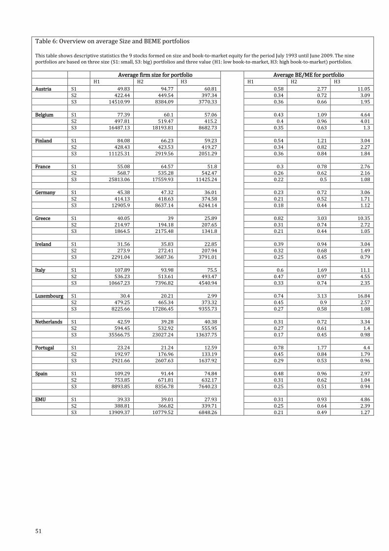
51
Table 6: Overview on average Size and BEME portfolios This table shows descriptive statistics the 9 stocks formed on size and book-to-market equity for the period July 1993 until June 2009. The nine portfolios are based on three size (S1: small, S3: big) portfolios and three value (H1: low book-to-market, H3: high book-to-market) portfolios.
Average firm size for portfolio Average BE/ME for portfolio H1 H2 H3 H1 H2 H3
Austria S1 49.83 94.77 60.81 0.58 2.77 11.05 S2 422.44 449.54 397.34 0.34 0.72 3.09 S3 14510.99 8384.09 3770.33 0.36 0.66 1.95 Belgium S1 77.39 60.1 57.06 0.43 1.09 4.64 S2 497.81 519.47 415.2 0.4 0.96 4.01 S3 16487.13 18193.81 8682.73 0.35 0.63 1.3 Finland S1 84.08 66.23 59.23 0.54 1.21 3.04 S2 428.43 423.53 419.27 0.34 0.82 2.27 S3 11125.31 2919.56 2051.29 0.36 0.84 1.84 France S1 55.08 64.57 51.8 0.3 0.78 2.76 S2 568.7 535.28 542.47 0.26 0.62 2.16 S3 25813.06 17559.93 11425.24 0.22 0.5 1.08 Germany S1 45.38 47.32 36.01 0.23 0.72 3.06 S2 414.13 418.63 374.58 0.21 0.52 1.71 S3 12905.9 8637.14 6244.14 0.18 0.44 1.12 Greece S1 40.05 39 25.89 0.82 3.03 10.35 S2 214.97 194.18 207.65 0.31 0.74 2.72 S3 1864.5 2175.48 1341.8 0.21 0.44 1.05 Ireland S1 31.56 35.83 22.85 0.39 0.94 3.04 S2 273.9 272.41 207.94 0.32 0.68 1.49 S3 2291.04 3687.36 3791.01 0.25 0.45 0.79 Italy S1 107.89 93.98 75.5 0.6 1.69 11.1 S2 536.23 513.61 493.47 0.47 0.97 4.55 S3 10667.23 7396.82 4540.94 0.33 0.74 2.35 Luxembourg S1 30.4 20.21 2.99 0.74 3.13 16.84 S2 479.25 465.34 373.32 0.45 0.9 2.57 S3 8225.66 17286.45 9355.73 0.27 0.58 1.08 Netherlands S1 42.59 39.28 40.38 0.31 0.72 3.34 S2 594.45 532.92 555.95 0.27 0.61 1.4 S3 35566.75 23027.24 13637.75 0.17 0.45 0.98 Portugal S1 23.24 21.24 12.59 0.78 1.77 4.4 S2 192.97 176.96 133.19 0.45 0.84 1.79 S3 2921.66 2607.63 1637.92 0.29 0.53 0.96 Spain S1 109.29 91.44 74.84 0.48 0.96 2.97 S2 753.85 671.81 632.17 0.31 0.62 1.04 S3 8893.85 8356.78 7640.23 0.25 0.51 0.94 EMU S1 39.33 39.01 27.93 0.31 0.93 4.86 S2 388.81 366.82 339.71 0.25 0.64 2.39 S3 13909.37 10779.52 6848.26 0.21 0.49 1.27
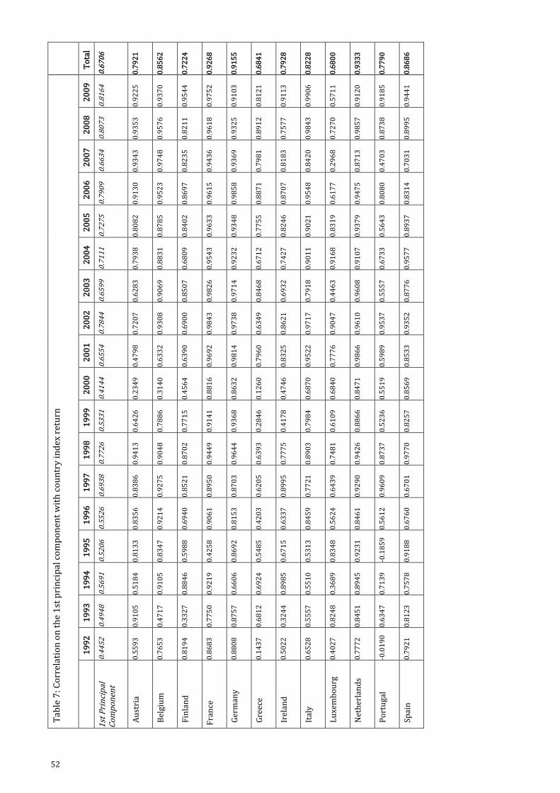
52
To
tal
0.6
70
6
0.7
92
1
0.8
56
2
0.7
22
4
0.9
26
8
0.9
15
5
0.6
84
1
0.7
92
8
0.8
22
8
0.6
80
0
0.9
33
3
0.7
79
0
0.8
68
6
Tab
le 7
: Co
rrel
atio
n o
n t
he
1st
pri
nci
pal
co
mp
on
ent
wit
h c
ou
ntr
y in
dex
ret
urn
20
09
0.8
16
4
0.9
22
5
0.9
37
0
0.9
54
4
0.9
75
2
0.9
10
3
0.8
12
1
0.9
11
3
0.9
90
6
0.5
71
1
0.9
12
0
0.9
18
5
0.9
44
1
20
08
0.8
07
3
0.9
35
3
0.9
57
6
0.8
21
1
0.9
61
8
0.9
32
5
0.8
91
2
0.7
57
7
0.9
84
3
0.7
27
0
0.9
85
7
0.8
73
8
0.8
99
5
20
07
0.6
63
4
0.9
34
3
0.9
74
8
0.8
23
5
0.9
43
6
0.9
36
9
0.7
98
1
0.8
18
3
0.8
42
0
0.2
96
8
0.8
71
3
0.4
70
3
0.7
03
1
20
06
0.7
90
9
0.9
13
0
0.9
52
3
0.8
69
7
0.9
61
5
0.9
85
8
0.8
87
1
0.8
70
7
0.9
54
8
0.6
17
7
0.9
47
5
0.8
08
0
0.8
31
4
20
05
0.7
27
5
0.8
08
2
0.8
78
5
0.8
40
2
0.9
63
3
0.9
34
8
0.7
75
5
0.8
24
6
0.9
02
1
0.8
31
9
0.9
37
9
0.5
64
3
0.8
93
7
20
04
0.7
11
1
0.7
93
8
0.8
83
1
0.6
80
9
0.9
54
3
0.9
23
2
0.6
71
2
0.7
42
7
0.9
01
1
0.9
16
8
0.9
10
7
0.6
73
3
0.9
57
7
20
03
0.6
59
9
0.6
28
3
0.9
06
9
0.8
50
7
0.9
82
6
0.9
71
4
0.8
46
8
0.6
93
2
0.7
91
8
0.4
46
3
0.9
60
8
0.5
55
7
0.8
77
6
20
02
0.7
84
4
0.7
20
7
0.9
30
8
0.6
90
0
0.9
84
3
0.9
73
8
0.6
34
9
0.8
62
1
0.9
71
7
0.9
04
7
0.9
61
0
0.9
53
7
0.9
35
2
20
01
0.6
55
4
0.4
79
8
0.6
33
2
0.6
39
0
0.9
69
2
0.9
81
4
0.7
96
0
0.8
32
5
0.9
52
2
0.7
77
6
0.9
86
6
0.5
98
9
0.8
53
3
20
00
0.4
14
4
0.2
34
9
0.3
14
0
0.4
56
4
0.8
81
6
0.8
63
2
0.1
26
0
0.4
74
6
0.6
87
0
0.6
84
0
0.8
47
1
0.5
51
9
0.8
56
9
19
99
0.5
33
1
0.6
42
6
0.7
88
6
0.7
71
5
0.9
14
1
0.9
36
8
0.2
84
6
0.4
17
8
0.7
98
4
0.6
10
9
0.8
86
6
0.5
23
6
0.8
25
7
19
98
0.7
72
6
0.9
41
3
0.9
04
8
0.8
70
2
0.9
44
9
0.9
64
4
0.6
39
3
0.7
77
5
0.8
90
3
0.7
48
1
0.9
42
6
0.8
73
7
0.9
77
0
19
97
0.6
93
8
0.8
38
6
0.9
27
5
0.8
52
1
0.8
95
0
0.8
70
3
0.6
20
5
0.8
99
5
0.7
72
1
0.6
43
9
0.9
29
0
0.9
60
9
0.6
70
1
19
96
0.5
52
6
0.8
35
6
0.9
21
4
0.6
94
0
0.9
06
1
0.8
15
3
0.4
20
3
0.6
33
7
0.8
45
9
0.5
62
4
0.8
46
1
0.5
61
2
0.6
76
0
19
95
0.5
20
6
0.8
13
3
0.8
34
7
0.5
98
8
0.4
25
8
0.8
69
2
0.5
48
5
0.6
71
5
0.5
31
3
0.8
34
8
0.9
23
1
-0.1
85
9
0.9
18
8
19
94
0.5
69
1
0.5
18
4
0.9
10
5
0.8
84
6
0.9
21
9
0.6
60
6
0.6
92
4
0.8
98
5
0.5
51
0
0.3
68
9
0.8
94
5
0.7
13
9
0.7
57
8
19
93
0.4
94
8
0.9
10
5
0.4
71
7
0.3
32
7
0.7
75
0
0.8
75
7
0.6
81
2
0.3
24
4
0.5
55
7
0.8
24
8
0.8
45
1
0.6
34
7
0.8
12
3
19
92
0.4
45
2
0.5
59
3
0.7
65
3
0.8
19
4
0.8
68
3
0.8
80
8
0.1
43
7
0.5
02
2
0.6
52
8
0.4
02
7
0.7
77
2
-0.0
19
0
0.7
92
1
1st
Pri
nci
pal
C
om
po
nen
t
Au
stri
a
Bel
giu
m
Fin
lan
d
Fra
nce
Ger
man
y
Gre
ece
Irel
and
Ital
y
Lu
xem
bo
urg
Net
her
lan
ds
Po
rtu
gal
Spai
n
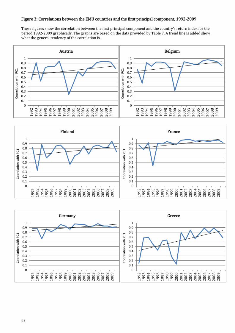
53
Figure 3: Correlations between the EMU countries and the first principal component, 1992-2009 These figures show the correlation between the first principal component and the country’s return index for the period 1992-2009 graphically. The graphs are based on the data provided by Table 7. A trend line is added show what the general tendency of the correlation is.
0
0.1
0.2
0.3
0.4
0.5
0.6
0.7
0.8
0.9
1
19
92
19
93
19
94
19
95
19
96
19
97
19
98
19
99
20
00
20
01
20
02
20
03
20
04
20
05
20
06
20
07
20
08
20
09
Co
ore
lati
on
wit
h P
C1
Austria
0
0.1
0.2
0.3
0.4
0.5
0.6
0.7
0.8
0.9
1
19
92
19
93
19
94
19
95
19
96
19
97
19
98
19
99
20
00
20
01
20
02
20
03
20
04
20
05
20
06
20
07
20
08
20
09
Co
ore
lati
on
wit
h P
C1
Belgium
0
0.1
0.2
0.3
0.4
0.5
0.6
0.7
0.8
0.9
1
19
92
19
93
19
94
19
95
19
96
19
97
19
98
19
99
20
00
20
01
20
02
20
03
20
04
20
05
20
06
20
07
20
08
20
09
Co
ore
lati
on
wit
h P
C1
Finland
0
0.1
0.2
0.3
0.4
0.5
0.6
0.7
0.8
0.9
11
99
21
99
31
99
41
99
51
99
61
99
71
99
81
99
92
00
02
00
12
00
22
00
32
00
42
00
52
00
62
00
72
00
82
00
9
Co
ore
lati
on
wit
h P
C1
France
0
0.1
0.2
0.3
0.4
0.5
0.6
0.7
0.8
0.9
1
19
92
19
93
19
94
19
95
19
96
19
97
19
98
19
99
20
00
20
01
20
02
20
03
20
04
20
05
20
06
20
07
20
08
20
09
Co
ore
lati
on
wit
h P
C1
Germany
0
0.1
0.2
0.3
0.4
0.5
0.6
0.7
0.8
0.9
1
19
92
19
93
19
94
19
95
19
96
19
97
19
98
19
99
20
00
20
01
20
02
20
03
20
04
20
05
20
06
20
07
20
08
20
09
Co
ore
lati
on
wit
h P
C1
Greece
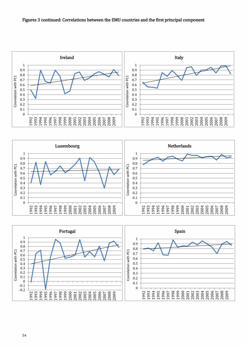
54
Figures 3 continued: Correlations between the EMU countries and the first principal component
0
0.1
0.2
0.3
0.4
0.5
0.6
0.7
0.8
0.9
1
19
92
19
93
19
94
19
95
19
96
19
97
19
98
19
99
20
00
20
01
20
02
20
03
20
04
20
05
20
06
20
07
20
08
20
09
Co
ore
lati
on
wit
h P
C1
Ireland
0
0.1
0.2
0.3
0.4
0.5
0.6
0.7
0.8
0.9
1
19
92
19
93
19
94
19
95
19
96
19
97
19
98
19
99
20
00
20
01
20
02
20
03
20
04
20
05
20
06
20
07
20
08
20
09
Co
ore
lati
on
wit
h P
C1
Italy
0
0.1
0.2
0.3
0.4
0.5
0.6
0.7
0.8
0.9
1
19
92
19
93
19
94
19
95
19
96
19
97
19
98
19
99
20
00
20
01
20
02
20
03
20
04
20
05
20
06
20
07
20
08
20
09
Co
ore
lati
on
wit
h P
C1
Luxembourg
0
0.1
0.2
0.3
0.4
0.5
0.6
0.7
0.8
0.9
1
19
92
19
93
19
94
19
95
19
96
19
97
19
98
19
99
20
00
20
01
20
02
20
03
20
04
20
05
20
06
20
07
20
08
20
09
Co
ore
lati
on
wit
h P
C1
Netherlands
-0.2-0.1
00.10.20.30.40.50.60.70.80.9
1
19
92
19
93
19
94
19
95
19
96
19
97
19
98
19
99
20
00
20
01
20
02
20
03
20
04
20
05
20
06
20
07
20
08
20
09
Co
ore
lati
on
wit
h P
C1
Portugal
0
0.1
0.2
0.3
0.4
0.5
0.6
0.7
0.8
0.9
1
19
92
19
93
19
94
19
95
19
96
19
97
19
98
19
99
20
00
20
01
20
02
20
03
20
04
20
05
20
06
20
07
20
08
20
09
Co
ore
lati
on
wit
h P
C1
Spain
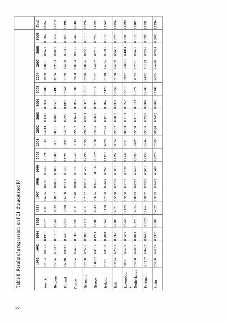
55
To
tal
0.6
25
7
0.7
31
8
0.5
19
6
0.8
58
2
0.8
37
4
0.4
65
5
0.6
26
7
0.6
75
4
0.4
59
8
0.8
70
5
0.6
05
1
0.7
53
4
Tab
le 8
: Res
ult
s o
f a
regr
essi
on
on
PC
1, t
he
adju
sted
R2
20
09
0.8
36
2
0.8
65
7
0.9
02
0
0.9
46
0
0.8
11
5
0.6
25
5
0.8
13
5
0.9
79
5
0.2
58
8
0.8
15
0
0.8
28
0
0.8
80
5
20
08
0.8
62
3
0.9
08
7
0.6
41
5
0.9
17
5
0.8
56
6
0.7
73
6
0.5
31
5
0.9
65
8
0.4
81
4
0.9
68
8
0.7
39
8
0.7
90
1
20
07
0.8
60
1
0.9
50
3
0.6
46
0
0.8
79
4
0.8
65
6
0.6
00
7
0.6
36
6
0.6
79
9
-0.0
03
1
0.7
35
1
0.1
43
3
0.4
43
8
20
06
0.8
17
0
0.8
97
6
0.7
32
0
0.9
16
8
0.9
69
0
0.7
65
7
0.7
33
8
0.9
02
8
0.3
19
7
0.8
87
5
0.6
18
2
0.6
60
3
20
05
0.6
18
5
0.7
48
9
0.6
76
6
0.9
20
8
0.8
61
3
0.5
61
6
0.6
47
9
0.7
95
2
0.6
61
3
0.8
67
6
0.2
50
3
0.7
78
6
20
04
0.5
93
1
0.7
57
9
0.4
09
9
0.9
01
7
0.8
37
6
0.3
95
5
0.5
06
7
0.7
93
2
0.8
24
6
0.8
12
4
0.3
98
7
0.9
08
8
20
03
0.3
34
3
0.8
04
6
0.6
96
0
0.9
62
1
0.9
38
1
0.6
88
8
0.4
28
5
0.5
89
7
0.1
19
1
0.9
15
5
0.2
39
7
0.7
47
2
20
02
0.4
71
3
0.8
53
1
0.4
23
7
0.9
65
7
0.9
43
2
0.3
43
4
0.7
17
4
0.9
38
7
0.8
00
3
0.9
16
0
0.9
00
5
0.8
62
0
20
01
0.1
53
2
0.3
41
1
0.3
49
2
0.9
33
3
0.9
59
5
0.5
97
0
0.6
62
3
0.8
97
4
0.5
65
1
0.9
70
7
0.2
94
6
0.7
00
9
20
00
-0.0
39
3
0.0
08
5
0.1
29
1
0.7
54
9
0.7
19
6
-0.0
82
5
0.1
47
8
0.4
19
2
0.4
14
7
0.6
89
3
0.2
35
0
0.7
07
8
19
99
0.3
54
2
0.5
84
2
0.5
54
6
0.8
19
2
0.8
65
3
-0.0
10
9
0.0
92
0
0.6
01
3
0.3
10
6
0.7
64
6
0.2
01
6
0.6
49
9
19
98
0.8
74
6
0.8
00
5
0.7
33
0
0.8
82
1
0.9
23
1
0.3
49
6
0.5
64
9
0.7
72
0
0.5
15
5
0.8
77
2
0.7
39
8
0.9
49
9
19
97
0.6
73
6
0.8
46
2
0.6
98
8
0.7
81
0
0.7
33
2
0.3
23
6
0.7
90
0
0.5
55
8
0.3
56
0
0.8
49
3
0.9
15
7
0.3
93
9
19
96
0.6
68
1
0.8
33
9
0.4
29
8
0.8
03
1
0.6
31
1
0.0
94
3
0.3
41
8
0.6
87
1
0.2
47
9
0.6
87
4
0.2
46
4
0.4
02
7
19
95
0.6
27
5
0.6
66
4
0.2
94
4
0.0
99
5
0.7
31
1
0.2
30
9
0.3
96
0
0.2
10
5
0.6
66
6
0.8
37
3
-0.0
62
0
0.8
28
6
19
94
0.1
95
6
0.8
11
8
0.7
60
8
0.8
34
9
0.3
80
0
0.4
27
4
0.7
88
1
0.2
34
0
0.0
49
7
0.7
80
1
0.4
60
6
0.5
31
6
19
93
0.8
12
0
0.1
44
7
0.0
21
7
0.5
60
6
0.7
43
6
0.4
10
5
0.0
15
8
0.2
39
7
0.6
48
3
0.6
85
7
0.3
43
2
0.6
25
9
19
92
0.2
36
4
0.5
39
6
0.6
34
8
0.7
26
6
0.7
50
8
-0.0
88
2
0.1
69
1
0.3
62
4
0.0
69
1
0.5
60
0
-0.1
10
7
0.5
86
0
Au
stri
a
Bel
giu
m
Fin
lan
d
Fra
nce
Ger
man
y
Gre
ece
Irel
and
Ital
y
Lu
xem
bo
ur
g Net
her
lan
ds
Po
rtu
gal
Spai
n
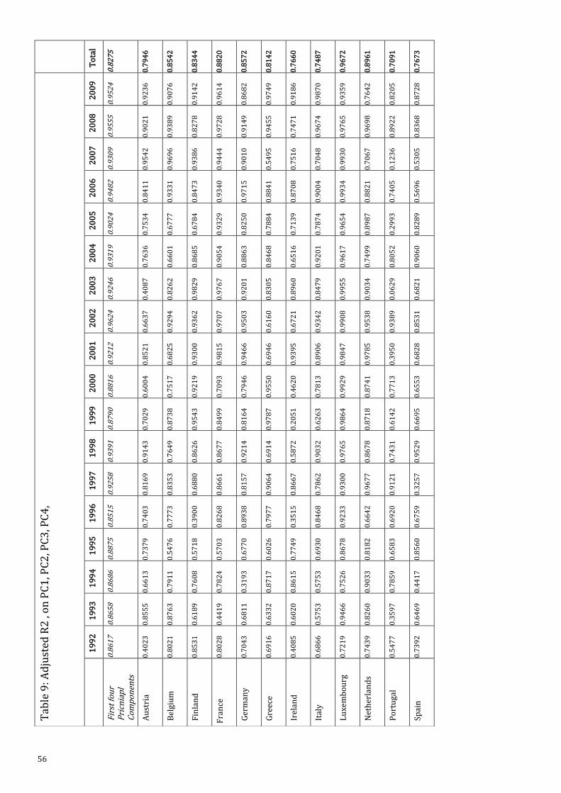
56
To
tal
0.8
27
5
0.7
94
6
0.8
54
2
0.8
34
4
0.8
82
0
0.8
57
2
0.8
14
2
0.7
66
0
0.7
48
7
0.9
67
2
0.8
96
1
0.7
09
1
0.7
67
3
Tab
le 9
: Ad
just
ed R
2 ,
on
PC
1, P
C2
, PC
3, P
C4
,
20
09
0.9
52
4
0.9
23
6
0.9
07
6
0.9
14
2
0.9
61
4
0.8
68
2
0.9
74
9
0.9
18
6
0.9
87
0
0.9
35
9
0.7
64
2
0.8
20
5
0.8
72
8
20
08
0.9
55
5
0.9
02
1
0.9
38
9
0.8
27
8
0.9
72
8
0.9
14
9
0.9
45
5
0.7
47
1
0.9
67
4
0.9
76
5
0.9
69
8
0.8
92
2
0.8
36
8
20
07
0.9
30
9
0.9
54
2
0.9
69
6
0.9
38
6
0.9
44
4
0.9
01
0
0.5
49
5
0.7
51
6
0.7
04
8
0.9
93
0
0.7
06
7
0.1
23
6
0.5
30
5
20
06
0.9
48
2
0.8
41
1
0.9
33
1
0.8
47
3
0.9
34
0
0.9
71
5
0.8
84
1
0.8
70
8
0.9
00
4
0.9
93
4
0.8
82
1
0.7
40
5
0.5
69
6
20
05
0.9
02
4
0.7
53
4
0.6
77
7
0.6
78
4
0.9
32
9
0.8
25
0
0.7
88
4
0.7
13
9
0.7
87
4
0.9
65
4
0.8
98
7
0.2
99
3
0.8
28
9
20
04
0.9
31
9
0.7
63
6
0.6
60
1
0.8
68
5
0.9
05
4
0.8
86
3
0.8
46
8
0.6
51
6
0.9
20
1
0.9
61
7
0.7
49
9
0.8
05
2
0.9
06
0
20
03
0.9
24
6
0.4
08
7
0.8
26
2
0.9
82
9
0.9
76
7
0.9
20
1
0.8
30
5
0.8
96
0
0.8
47
9
0.9
95
5
0.9
03
4
0.0
62
9
0.6
82
1
20
02
0.9
62
4
0.6
63
7
0.9
29
4
0.9
36
2
0.9
70
7
0.9
50
3
0.6
16
0
0.6
72
1
0.9
34
2
0.9
90
8
0.9
53
8
0.9
38
9
0.8
53
1
20
01
0.9
21
2
0.8
52
1
0.6
82
5
0.9
30
0
0.9
81
5
0.9
46
6
0.6
94
6
0.9
39
5
0.8
90
6
0.9
84
7
0.9
78
5
0.3
95
0
0.6
82
8
20
00
0.8
81
6
0.6
00
4
0.7
51
7
0.9
21
9
0.7
09
3
0.7
94
6
0.9
55
0
0.4
62
0
0.7
81
3
0.9
92
9
0.8
74
1
0.7
71
3
0.6
55
3
19
99
0.8
79
0
0.7
02
9
0.8
73
8
0.9
54
3
0.8
49
9
0.8
16
4
0.9
78
7
0.2
05
1
0.6
26
3
0.9
86
4
0.8
71
8
0.6
14
2
0.6
69
5
19
98
0.9
39
1
0.9
14
3
0.7
64
9
0.8
62
6
0.8
67
7
0.9
21
4
0.6
91
4
0.5
87
2
0.9
03
2
0.9
76
5
0.8
67
8
0.7
43
1
0.9
52
9
19
97
0.9
25
8
0.8
16
9
0.8
35
3
0.6
88
0
0.8
66
1
0.8
15
7
0.9
06
4
0.8
66
7
0.7
86
2
0.9
30
0
0.9
67
7
0.9
12
1
0.3
25
7
19
96
0.8
51
5
0.7
40
3
0.7
77
3
0.3
90
0
0.8
26
8
0.8
93
8
0.7
97
7
0.3
51
5
0.8
46
8
0.9
23
3
0.6
64
2
0.6
92
0
0.6
75
9
19
95
0.8
87
5
0.7
37
9
0.5
47
6
0.5
71
8
0.5
70
3
0.6
77
0
0.6
02
6
0.7
74
9
0.6
93
0
0.8
67
8
0.8
18
2
0.6
58
3
0.8
56
0
19
94
0.8
68
6
0.6
61
3
0.7
91
1
0.7
60
8
0.7
82
4
0.3
19
3
0.8
71
7
0.8
61
5
0.5
75
3
0.7
52
6
0.9
03
3
0.7
85
9
0.4
41
7
19
93
0.8
65
8
0.8
55
5
0.8
76
3
0.6
18
9
0.4
41
9
0.6
81
1
0.6
33
2
0.6
02
0
0.5
75
3
0.9
46
6
0.8
26
0
0.3
59
7
0.6
46
9
19
92
0.8
61
7
0.4
02
3
0.8
02
1
0.8
53
1
0.8
02
8
0.7
04
3
0.6
91
6
0.4
08
5
0.6
86
6
0.7
21
9
0.7
43
9
0.5
47
7
0.7
39
2
Fir
st fo
ur
Pri
cnia
pl
Co
mp
on
ents
Au
stri
a
Bel
giu
m
Fin
lan
d
Fra
nce
Ger
man
y
Gre
ece
Irel
and
Ital
y
Lu
xem
bo
urg
Net
her
lan
ds
Po
rtu
gal
Spai
n
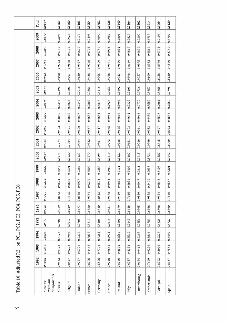
57
To
tal
0.8
99
4
0.8
65
3
0.8
66
0
0.9
18
3
0.8
95
4
0.8
75
2
0.9
92
8
0.9
64
0
0.7
80
4
0.9
80
2
0.9
01
4
0.9
06
4
0.8
12
9
Tab
le 1
0: A
dju
sted
R2
, o
n P
C1
, PC
2, P
C3
, PC
4, P
C5
, PC
6
20
09
0.9
81
2
0.9
59
6
0.8
92
5
0.9
17
7
0.9
49
5
0.8
69
9
0.9
98
2
0.9
80
3
0.9
82
7
0.9
30
0
0.6
73
7
0.9
10
4
0.8
70
9
20
08
0.9
86
7
0.9
73
0
0.9
19
8
0.9
60
9
0.9
70
2
0.9
75
0
0.9
99
3
0.9
83
2
0.9
66
9
0.9
89
0
0.9
81
9
0.9
79
2
0.8
73
0
20
07
0.9
76
6
0.9
72
2
0.9
67
8
0.9
92
7
0.9
74
6
0.9
39
9
0.9
97
1
0.9
68
0
0.8
16
9
0.9
97
5
0.8
98
2
0.8
96
6
0.4
54
0
20
06
0.9
84
3
0.9
19
8
0.9
20
7
0.9
12
0
0.9
42
6
0.9
79
5
0.9
96
6
0.9
72
3
0.9
59
8
0.9
95
7
0.9
10
9
0.8
95
8
0.5
13
0
20
05
0.9
67
4
0.7
39
0
0.8
80
1
0.7
91
6
0.9
36
1
0.8
11
6
0.9
95
1
0.9
69
2
0.9
10
9
0.9
73
6
0.8
65
7
0.8
86
8
0.7
79
8
20
04
0.9
84
5
0.8
34
4
0.6
03
4
0.9
34
2
0.9
80
2
0.8
81
6
0.9
92
8
0.8
99
8
0.9
32
8
0.9
77
9
0.7
58
7
0.9
06
1
0.9
56
0
20
03
0.9
87
2
0.3
83
0
0.8
86
8
0.9
89
7
0.9
68
6
0.9
65
1
0.9
98
1
0.9
85
9
0.9
64
1
0.9
96
6
0.9
45
9
0.9
50
8
0.8
55
8
20
02
0.9
88
0
0.9
40
2
0.9
49
1
0.9
80
0
0.9
86
7
0.9
41
7
0.9
98
5
0.9
85
5
0.9
50
3
0.9
94
1
0.9
95
3
0.9
59
7
0.8
99
2
20
01
0.9
76
0
0.7
97
4
0.7
00
4
0.9
79
4
0.9
82
2
0.9
50
1
0.9
97
3
0.9
83
8
0.9
66
1
0.9
94
0
0.9
79
0
0.8
61
5
0.8
00
0
20
00
0.9
66
4
0.6
07
3
0.9
03
0
0.9
13
3
0.9
57
0
0.8
19
4
0.9
91
9
0.9
42
1
0.7
48
7
0.9
91
5
0.8
73
1
0.9
58
7
0.7
04
2
19
99
0.9
58
1
0.8
64
4
0.8
59
1
0.9
38
4
0.8
60
7
0.9
28
7
0.9
96
0
0.9
13
1
0.5
40
8
0.9
81
1
0.9
63
5
0.8
10
8
0.7
20
1
19
98
0.9
81
1
0.9
52
4
0.8
64
6
0.9
92
7
0.9
29
9
0.9
59
4
0.9
98
4
0.9
88
0
0.8
83
1
0.9
94
7
0.8
40
0
0.9
84
8
0.9
53
7
19
97
0.9
71
0
0.8
17
3
0.7
96
5
0.8
83
8
0.9
36
4
0.8
51
3
0.9
97
8
0.9
45
9
0.7
14
6
0.9
55
9
0.9
55
8
0.9
32
4
0.7
82
6
19
96
0.9
72
0
0.9
01
9
0.8
22
9
0.8
47
7
0.8
53
0
0.8
54
0
0.9
83
1
0.8
57
9
0.8
44
8
0.9
79
5
0.6
26
6
0.6
80
6
0.6
59
0
19
95
0.9
79
1
0.9
70
6
0.8
91
7
0.9
70
5
0.8
61
9
0.8
40
6
0.9
91
8
0.9
50
8
0.9
64
3
0.9
85
1
0.9
78
9
0.6
62
8
0.8
72
2
19
94
0.9
65
4
0.7
12
3
0.7
99
7
0.9
33
5
0.7
83
7
0.7
36
1
0.9
97
1
0.9
56
6
0.8
51
9
0.9
30
7
0.8
81
4
0.9
32
7
0.6
49
9
19
93
0.9
54
9
0.9
17
3
0.9
20
3
0.5
79
6
0.4
46
3
0.7
79
2
0.9
63
1
0.8
57
4
0.4
38
1
0.9
41
3
0.9
27
9
0.8
02
9
0.7
53
1
19
92
0.9
69
2
0.9
43
3
0.8
44
7
0.9
72
7
0.8
70
6
0.5
89
6
0.9
72
6
0.8
76
6
0.6
73
7
0.9
18
4
0.7
69
9
0.8
79
3
0.8
13
7
Fir
st s
ix
Pri
cnia
pl
Co
mp
on
ents
Au
stri
a
Bel
giu
m
Fin
lan
d
Fra
nce
Ger
man
y
Gre
ece
Irel
and
Ital
y
Lu
xem
bo
urg
Net
her
lan
ds
Po
rtu
gal
Spai
n
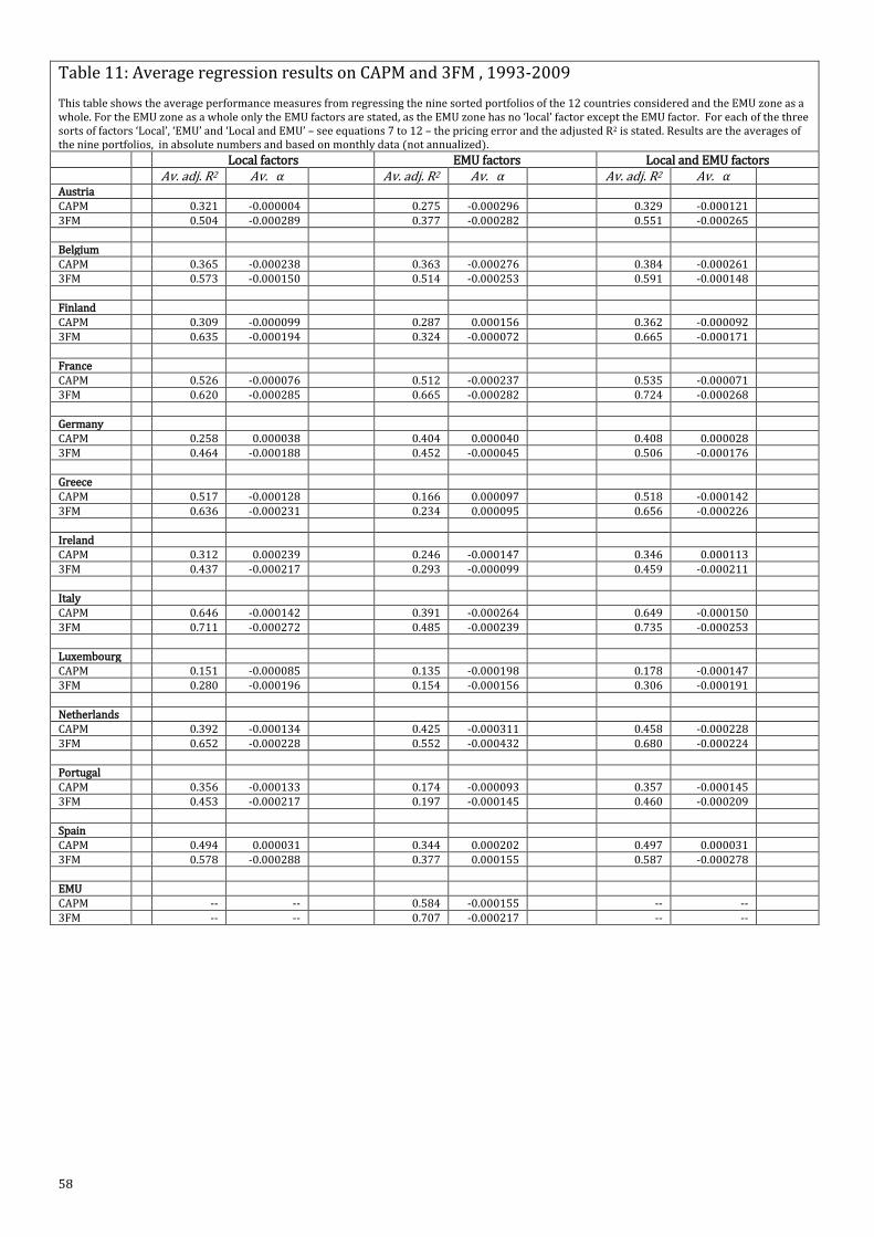
58
Table 11: Average regression results on CAPM and 3FM , 1993-2009 This table shows the average performance measures from regressing the nine sorted portfolios of the 12 countries considered and the EMU zone as a whole. For the EMU zone as a whole only the EMU factors are stated, as the EMU zone has no ‘local’ factor except the EMU factor. For each of the three sorts of factors ‘Local’, ‘EMU’ and ‘Local and EMU’ – see equations 7 to 12 – the pricing error and the adjusted R2 is stated. Results are the averages of the nine portfolios, in absolute numbers and based on monthly data (not annualized).
Local factors EMU factors Local and EMU factors Av. adj. R2 Av. Av. adj. R2 Av. Av. adj. R2 Av. Austria CAPM 0.321 -0.000004 0.275 -0.000296 0.329 -0.000121 3FM 0.504 -0.000289 0.377 -0.000282 0.551 -0.000265 Belgium CAPM 0.365 -0.000238 0.363 -0.000276 0.384 -0.000261 3FM 0.573 -0.000150 0.514 -0.000253 0.591 -0.000148 Finland CAPM 0.309 -0.000099 0.287 0.000156 0.362 -0.000092 3FM 0.635 -0.000194 0.324 -0.000072 0.665 -0.000171 France CAPM 0.526 -0.000076 0.512 -0.000237 0.535 -0.000071 3FM 0.620 -0.000285 0.665 -0.000282 0.724 -0.000268 Germany CAPM 0.258 0.000038 0.404 0.000040 0.408 0.000028 3FM 0.464 -0.000188 0.452 -0.000045 0.506 -0.000176 Greece CAPM 0.517 -0.000128 0.166 0.000097 0.518 -0.000142 3FM 0.636 -0.000231 0.234 0.000095 0.656 -0.000226 Ireland CAPM 0.312 0.000239 0.246 -0.000147 0.346 0.000113 3FM 0.437 -0.000217 0.293 -0.000099 0.459 -0.000211 Italy CAPM 0.646 -0.000142 0.391 -0.000264 0.649 -0.000150 3FM 0.711 -0.000272 0.485 -0.000239 0.735 -0.000253 Luxembourg CAPM 0.151 -0.000085 0.135 -0.000198 0.178 -0.000147 3FM 0.280 -0.000196 0.154 -0.000156 0.306 -0.000191 Netherlands CAPM 0.392 -0.000134 0.425 -0.000311 0.458 -0.000228 3FM 0.652 -0.000228 0.552 -0.000432 0.680 -0.000224 Portugal CAPM 0.356 -0.000133 0.174 -0.000093 0.357 -0.000145 3FM 0.453 -0.000217 0.197 -0.000145 0.460 -0.000209 Spain CAPM 0.494 0.000031 0.344 0.000202 0.497 0.000031 3FM 0.578 -0.000288 0.377 0.000155 0.587 -0.000278 EMU CAPM -- -- 0.584 -0.000155 -- -- 3FM -- -- 0.707 -0.000217 -- --

59
Table 12: Regression results on CAPM, 1993-2009 This table shows the monthly performance measures from regressing the nine sorted portfolios of the 12 countries considered and the EMU zone as a whole. For the EMU zone as a whole only the CAPM (EMU) is stated, as the EMU zone has no ‘local’ factor except the EMU factor. For each of the three models CAPM (local), CAPM (EMU) and CAPM (local and EMU) – see equations 7, 9 and 11 – the pricing error and the adjusted R2 is stated. Results are in absolute numbers, based on monthly data (not annualized).
CAPM (local) CAPM (EMU ) CAPM (local and EMU) Adj. R2 Adj. R2 Adj. R2
Austria S3H3 0.355 0.000829 0.311 0.000519 0.365 0.000705 S3H2 0.509 0.001340 0.428 0.000383 0.519 0.001020 S3H1 0.565 -0.002000 0.519 -0.003100 0.592 -0.002520 S2H3 0.252 0.000134 0.176 0.000083 0.248 0.000132 S2H2 0.329 -0.000127 0.349 -0.000233 0.368 -0.000197 S2H1 0.288 -0.000145 0.223 -0.000217 0.286 -0.000160 S1H3 0.128 0.000010 0.121 0.000000 0.132 0.000005 S1H2 0.237 -0.000068 0.190 -0.000085 0.236 -0.000072 S1H1 0.223 -0.000005 0.160 -0.000014 0.219 -0.000005
Belgium S3H3 0.474 0.000203 0.496 0.000097 0.507 0.000114 S3H2 0.715 -0.001610 0.675 -0.001780 0.730 -0.001720 S3H1 0.611 -0.000761 0.498 -0.000810 0.609 -0.000756 S2H3 0.216 0.000006 0.216 0.000002 0.222 0.000003 S2H2 0.296 0.000010 0.319 0.000002 0.321 0.000003 S2H1 0.398 0.000007 0.417 0.000001 0.425 0.000002 S1H3 0.152 0.000000 0.179 0.000000 0.175 0.000000 S1H2 0.214 0.000004 0.243 0.000003 0.240 0.000003 S1H1 0.206 0.000002 0.224 0.000001 0.223 0.000001
Finland S3H3 0.277 0.000339 0.338 0.000297 0.352 0.000247 S3H2 0.409 0.000378 0.527 0.000271 0.544 0.000193 S3H1 0.864 -0.002250 0.351 0.000203 0.892 -0.001840 S2H3 0.290 0.000166 0.329 0.000160 0.351 0.000145 S2H2 0.238 0.000307 0.244 0.000308 0.271 0.000286 S2H1 0.298 0.000060 0.336 0.000055 0.360 0.000041 S1H3 0.128 0.000027 0.120 0.000028 0.138 0.000025 S1H2 0.100 0.000051 0.150 0.000048 0.147 0.000047 S1H1 0.180 0.000031 0.188 0.000031 0.206 0.000028
France S3H3 0.793 0.000166 0.762 -0.000167 0.796 0.000072 S3H2 0.887 -0.000756 0.814 -0.001250 0.887 -0.000732 S3H1 0.856 -0.000179 0.764 -0.000742 0.859 -0.000023 S2H3 0.443 0.000003 0.461 -0.000015 0.460 -0.000011 S2H2 0.516 -0.000005 0.518 -0.000025 0.525 -0.000017 S2H1 0.520 0.000079 0.519 0.000061 0.528 0.000070 S1H3 0.226 -0.000001 0.255 -0.000003 0.252 -0.000003 S1H2 0.262 0.000003 0.279 0.000001 0.275 0.000002 S1H1 0.233 0.000006 0.235 0.000004 0.235 0.000005
Germany S3H3 0.432 0.000051 0.538 0.000095 0.550 0.000035 S3H2 0.610 -0.000725 0.809 -0.000679 0.818 -0.000755 S3H1 0.370 0.000821 0.602 0.000770 0.600 0.000785 S2H3 0.319 0.000048 0.535 0.000045 0.534 0.000046 S2H2 0.321 0.000061 0.513 0.000059 0.511 0.000059 S2H1 0.136 0.000057 0.289 0.000049 0.295 0.000055 S1H3 0.049 0.000012 0.101 0.000011 0.098 0.000011 S1H2 0.077 0.000012 0.200 0.000011 0.212 0.000012 S1H1 0.006 0.000002 0.046 0.000001 0.057 0.000002
Greece S3H3 0.764 0.000369 0.243 0.000800 0.763 0.000376 S3H2 0.828 -0.001300 0.350 -0.000656 0.835 -0.001470 S3H1 0.635 -0.000348 0.194 0.000272 0.634 -0.000323 S2H3 0.614 0.000035 0.262 0.000090 0.618 0.000019 S2H2 0.614 -0.000073 0.175 0.000044 0.613 -0.000064 S2H1 0.563 0.000134 0.135 0.000249 0.566 0.000151 S1H3 0.130 -0.000017 0.029 -0.000013 0.127 -0.000017 S1H2 0.309 -0.000045 0.077 -0.000029 0.307 -0.000043 S1H1 0.197 0.000090 0.033 0.000113 0.199 0.000096
Ireland S3H3 0.508 -0.000166 0.300 -0.001240 0.519 -0.000461 S3H2 0.528 0.000529 0.320 -0.000853 0.542 0.000125 S3H1 0.477 0.000959 0.299 0.000310 0.492 0.000753 S2H3 0.218 0.000211 0.240 0.000113 0.276 0.000147 S2H2 0.319 0.000202 0.338 0.000088 0.397 0.000129 S2H1 0.361 0.000304 0.365 0.000176 0.439 0.000226 S1H3 0.175 0.000019 0.152 0.000011 0.197 0.000015 S1H2 0.119 0.000060 0.111 0.000048 0.137 0.000053 S1H1 0.101 0.000037 0.089 0.000025 0.112 0.000031
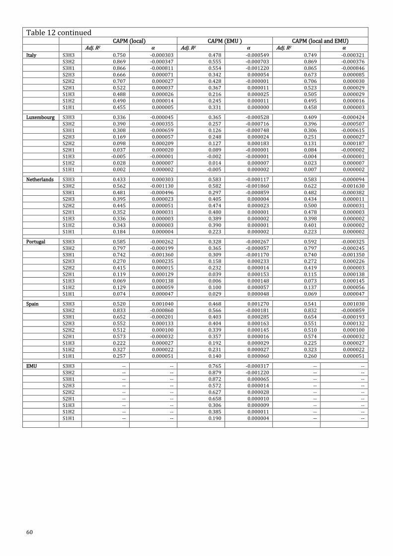
60
Table 12 continued CAPM (local) CAPM (EMU ) CAPM (local and EMU) Adj. R2 Adj. R2 Adj. R2
Italy S3H3 0.750 -0.000303 0.478 -0.000549 0.749 -0.000321 S3H2 0.869 -0.000347 0.555 -0.000703 0.869 -0.000376 S3H1 0.866 -0.000811 0.554 -0.001220 0.865 -0.000846 S2H3 0.666 0.000071 0.342 0.000054 0.673 0.000085 S2H2 0.707 0.000027 0.428 -0.000001 0.706 0.000030 S2H1 0.522 0.000037 0.367 0.000011 0.523 0.000029 S1H3 0.488 0.000026 0.216 0.000025 0.505 0.000029 S1H2 0.490 0.000014 0.245 0.000011 0.495 0.000016 S1H1 0.455 0.000005 0.331 0.000000 0.458 0.000003
Luxembourg S3H3 0.336 -0.000045 0.365 -0.000528 0.409 -0.000424 S3H2 0.390 -0.000355 0.257 -0.000716 0.396 -0.000507 S3H1 0.308 -0.000659 0.126 -0.000748 0.306 -0.000615 S2H3 0.169 0.000057 0.248 0.000024 0.251 0.000027 S2H2 0.098 0.000209 0.127 0.000183 0.131 0.000187 S2H1 0.037 0.000020 0.089 -0.000001 0.084 -0.000002 S1H3 -0.005 -0.000001 -0.002 -0.000001 -0.004 -0.000001 S1H2 0.028 0.000007 0.014 0.000007 0.023 0.000007 S1H1 0.002 0.000002 -0.005 0.000002 0.007 0.000002
Netherlands S3H3 0.433 0.000303 0.583 -0.000117 0.583 -0.000094 S3H2 0.562 -0.001130 0.582 -0.001860 0.622 -0.001630 S3H1 0.481 -0.000496 0.297 -0.000859 0.482 -0.000382 S2H3 0.395 0.000023 0.405 0.000004 0.434 0.000011 S2H2 0.445 0.000051 0.474 0.000023 0.500 0.000031 S2H1 0.352 0.000031 0.480 0.000001 0.478 0.000003 S1H3 0.336 0.000003 0.389 0.000002 0.398 0.000002 S1H2 0.343 0.000003 0.390 0.000001 0.401 0.000002 S1H1 0.184 0.000004 0.223 0.000002 0.223 0.000002
Portugal S3H3 0.585 -0.000262 0.328 -0.000267 0.592 -0.000325 S3H2 0.797 -0.000199 0.365 -0.000057 0.797 -0.000245 S3H1 0.742 -0.001360 0.309 -0.001170 0.740 -0.001350 S2H3 0.270 0.000235 0.158 0.000233 0.272 0.000226 S2H2 0.415 0.000015 0.232 0.000014 0.419 0.000003 S2H1 0.119 0.000129 0.039 0.000153 0.115 0.000138 S1H3 0.069 0.000138 0.006 0.000148 0.073 0.000145 S1H2 0.129 0.000059 0.100 0.000057 0.137 0.000056 S1H1 0.074 0.000047 0.029 0.000048 0.069 0.000047
Spain S3H3 0.520 0.001040 0.468 0.001270 0.541 0.001030 S3H2 0.833 -0.000860 0.566 -0.000181 0.832 -0.000859 S3H1 0.652 -0.000201 0.403 0.000285 0.654 -0.000193 S2H3 0.552 0.000133 0.404 0.000163 0.551 0.000132 S2H2 0.512 0.000100 0.339 0.000145 0.510 0.000100 S2H1 0.573 -0.000032 0.357 0.000016 0.574 -0.000032 S1H3 0.222 0.000027 0.192 0.000029 0.225 0.000027 S1H2 0.327 0.000022 0.231 0.000027 0.323 0.000022 S1H1 0.257 0.000051 0.140 0.000060 0.260 0.000051
EMU S3H3 -- -- 0.765 -0.000317 -- -- S3H2 -- -- 0.879 -0.001220 -- -- S3H1 -- -- 0.872 0.000065 -- -- S2H3 -- -- 0.572 0.000014 -- -- S2H2 -- -- 0.627 0.000028 -- -- S2H1 -- -- 0.658 0.000010 -- -- S1H3 -- -- 0.306 0.000009 -- -- S1H2 -- -- 0.385 0.000011 -- -- S1H1 -- -- 0.190 0.000004 -- --
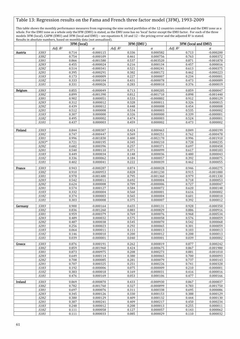
61
Table 13: Regression results on the Fama and French three factor model (3FM), 1993-2009 This table shows the monthly performance measures from regressing the nine sorted portfolios of the 12 countries considered and the EMU zone as a whole. For the EMU zone as a whole only the3FM (EMU) is stated, as the EMU zone has no ‘local’ factor except the EMU factor. For each of the three models 3FM (local), CAPM (EMU) and 3FM (local and EMU) – see equations 8, 10 and 12 – the pricing error and the adjusted R2 is stated. Results in absolute numbers, based on monthly data (not annualized).
3FM (local) 3FM (EMU ) 3FM (local and EMU) Adj. R2 Adj. R2 Adj. R2 Austria S3H3 0.714 -0.000115 0.336 0.000582 0.713 -0.000200 S3H2 0.754 -0.000109 0.461 0.000756 0.763 0.000372 S3H1 0.866 -0.001580 0.537 -0.003520 0.871 -0.001870 S2H3 0.455 -0.000024 0.216 0.000134 0.457 0.000016 S2H2 0.514 -0.000341 0.521 -0.000241 0.613 -0.000375 S2H1 0.395 -0.000291 0.382 -0.000172 0.462 -0.000223 S1H3 0.173 -0.000009 0.227 0.000007 0.234 -0.000001 S1H2 0.333 -0.000104 0.431 -0.000078 0.473 -0.000089 S1H1 0.331 -0.000026 0.283 -0.000010 0.376 -0.000019
Belgium S3H3 0.855 -0.000049 0.713 0.000205 0.859 -0.000047 S3H2 0.899 -0.001390 0.812 -0.001710 0.898 -0.001440 S3H1 0.902 0.000051 0.533 -0.000802 0.912 0.000129 S2H3 0.312 0.000012 0.328 0.000011 0.326 0.000015 S2H2 0.439 0.000012 0.448 0.000008 0.454 0.000008 S2H1 0.512 0.000008 0.534 0.000003 0.535 0.000002 S1H3 0.307 0.000000 0.326 0.000000 0.339 -0.000001 S1H2 0.495 0.000002 0.474 0.000003 0.524 0.000001 S1H1 0.437 0.000003 0.459 0.000002 0.473 0.000002
Finland S3H3 0.844 -0.000307 0.424 0.000463 0.849 -0.000199 S3H2 0.747 -0.000447 0.569 0.000251 0.762 -0.000478 S3H1 0.996 -0.001830 0.400 -0.002170 0.996 -0.001910 S2H3* 0.721 0.000195 0.345 0.000210 0.728 0.000235 S2H2 0.682 0.000396 0.257 0.000371 0.697 0.000458 S2H1 0.540 0.000110 0.371 0.000099 0.617 0.000183 S1H3 0.449 0.000034 0.148 0.000036 0.480 0.000043 S1H2 0.336 0.000062 0.184 0.000057 0.392 0.000075 S1H1 0.402 0.000041 0.222 0.000039 0.462 0.000055
France S3H3 0.943 -0.000287 0.874 -0.000028 0.946 -0.000275 S3H2 0.910 -0.000953 0.828 -0.001230 0.915 -0.001080 S3H1 0.978 -0.001480 0.795 -0.001360 0.979 -0.001330 S2H3 0.542 0.000011 0.692 0.000004 0.718 0.000053 S2H2 0.624 0.000008 0.709 -0.000006 0.727 0.000047 S2H1 0.574 0.000127 0.584 0.000072 0.620 0.000148 S1H3 0.332 -0.000004 0.560 -0.000001 0.616 0.000002 S1H2 0.374 0.000003 0.565 0.000004 0.601 0.000010 S1H1 0.303 0.000008 0.375 0.000007 0.392 0.000012
Germany S3H3 0.900 -0.000164 0.655 0.000131 0.928 -0.000350 S3H2 0.836 -0.001260 0.883 -0.000829 0.886 -0.000916 S3H1 0.959 -0.000379 0.769 0.000076 0.968 -0.000534 S2H3 0.489 0.000032 0.575 0.000058 0.576 0.000059 S2H2 0.487 0.000038 0.545 0.000070 0.542 0.000068 S2H1 0.256 0.000023 0.292 0.000065 0.301 0.000059 S1H3 0.064 0.000011 0.111 0.000013 0.103 0.000013 S1H2 0.146 0.000010 0.200 0.000012 0.208 0.000013 S1H1 0.039 -0.000001 0.040 0.000001 0.039 0.000002
Greece S3H3 0.876 0.000191 0.262 0.000819 0.877 0.000242 S3H2 0.859 -0.001960 0.424 -0.000675 0.867 -0.001980 S3H1 0.873 -0.000975 0.208 0.000273 0.881 -0.001010 S2H3 0.649 0.000114 0.380 0.000065 0.700 0.000093 S2H2 0.708 0.000085 0.281 0.000079 0.737 0.000143 S2H1 0.707 0.000325 0.251 0.000226 0.741 0.000328 S1H3 0.192 -0.000006 0.075 -0.000009 0.210 -0.000001 S1H2 0.383 -0.000018 0.169 -0.000031 0.416 -0.000016 S1H1 0.476 0.000169 0.053 0.000106 0.477 0.000166
Ireland S3H3 0.869 -0.000870 0.433 -0.000930 0.867 -0.000837 S3H2 0.782 -0.001760 0.327 -0.000899 0.783 -0.001750 S3H1 0.697 0.000076 0.311 0.000338 0.695 0.000086 S2H3 0.345 0.000126 0.330 0.000153 0.388 0.000129 S2H2 0.380 0.000129 0.409 0.000132 0.444 0.000130 S2H1 0.387 0.000241 0.409 0.000217 0.450 0.000234 S1H3 0.248 0.000012 0.208 0.000013 0.255 0.000011 S1H2 0.111 0.000058 0.127 0.000057 0.143 0.000062 S1H1 0.111 0.000033 0.085 0.000029 0.110 0.000032

62
Table 12 continued 3FM (local) 3FM (EMU ) 3FM (local and EMU) Adj. R2 Adj. R2 Adj. R2 Italy S3H3 0.932 -0.000860 0.602 -0.000332 0.935 -0.000917 S3H2 0.871 -0.000613 0.570 -0.000488 0.872 -0.000476 S3H1 0.958 -0.001260 0.561 -0.001610 0.958 -0.001290 S2H3 0.718 0.000107 0.425 0.000111 0.728 0.000141 S2H2 0.750 0.000057 0.528 0.000055 0.764 0.000092 S2H1 0.538 0.000054 0.456 0.000049 0.571 0.000084 S1H3 0.562 0.000034 0.321 0.000030 0.582 0.000037 S1H2 0.557 0.000023 0.379 0.000024 0.589 0.000033 S1H1 0.513 0.000011 0.526 0.000010 0.613 0.000020
Luxembourg S3H3 0.614 -0.001210 0.441 -0.000352 0.675 -0.001220 S3H2 0.590 -0.001010 0.265 -0.000591 0.622 -0.000995 S3H1 0.765 0.000261 0.117 -0.000705 0.764 0.000309 S2H3 0.284 0.000007 0.300 0.000037 0.350 0.000004 S2H2 0.183 0.000166 0.119 0.000189 0.180 0.000157 S2H1 0.049 0.000013 0.122 0.000009 0.119 0.000011 S1H3 -0.001 0.000000 0.007 0.000000 0.007 0.000000 S1H2 0.044 0.000007 0.019 0.000008 0.042 0.000008 S1H1 -0.006 0.000002 -0.008 0.000002 -0.004 0.000003
Netherlands S3H3 0.829 0.000022 0.655 -0.000202 0.844 -0.000013 S3H2 0.887 -0.001650 0.743 -0.002190 0.893 -0.001620 S3H1 0.949 -0.000486 0.371 -0.001540 0.949 -0.000462 S2H3 0.577 0.000011 0.510 0.000007 0.593 0.000023 S2H2 0.687 0.000032 0.666 0.000022 0.729 0.000039 S2H1 0.560 0.000014 0.641 0.000005 0.642 0.000010 S1H3 0.510 0.000003 0.507 0.000002 0.539 0.000003 S1H2 0.556 0.000002 0.555 0.000002 0.598 0.000003 S1H1 0.309 0.000003 0.320 0.000003 0.329 0.000003
Portugal S3H3 0.749 -0.000581 0.372 -0.000242 0.748 -0.000540 S3H2 0.848 -0.000857 0.425 -0.000427 0.849 -0.000966 S3H1 0.932 -0.001020 0.306 -0.001390 0.932 -0.001000 S2H3 0.428 0.000241 0.218 0.000278 0.464 0.000285 S2H2 0.466 -0.000025 0.273 0.000065 0.487 0.000029 S2H1 0.184 0.000007 0.039 0.000165 0.182 0.000034 S1H3 0.145 0.000169 -0.002 0.000138 0.137 0.000162 S1H2 0.210 0.000059 0.113 0.000057 0.221 0.000058 S1H1 0.118 0.000052 0.027 0.000053 0.117 0.000055
Spain S3H3 0.913 -0.000079 0.642 0.001240 0.915 0.000005 S3H2 0.869 -0.001580 0.575 -0.000613 0.870 -0.001760 S3H1 0.855 -0.001050 0.406 0.000265 0.860 -0.000942 S2H3 0.610 0.000073 0.450 0.000175 0.614 0.000097 S2H2 0.534 0.000041 0.367 0.000181 0.555 0.000084 S2H1 0.585 -0.000078 0.371 0.000020 0.589 -0.000064 S1H3 0.230 0.000022 0.203 0.000032 0.237 0.000026 S1H2 0.346 0.000014 0.246 0.000033 0.362 0.000019 S1H1 0.259 0.000041 0.132 0.000059 0.281 0.000036
EMU S3H3 -- -- 0.975 -0.000198 -- -- S3H2 -- -- 0.972 -0.001330 -- -- S3H1 -- -- 0.984 -0.000535 -- -- S2H3 -- -- 0.780 0.000029 -- -- S2H2 -- -- 0.806 0.000042 -- -- S2H1 -- -- 0.795 0.000017 -- -- S1H3 -- -- 0.400 0.000010 -- -- S1H2 -- -- 0.461 0.000012 -- -- S1H1 -- -- 0.194 0.000004 -- --

63
Table 14: Comparing the average regression results on CAPM and 3FM of pre- and post-2001 This table shows the average performance measures from regressing the nine sorted portfolios of the 12 countries considered and the EMU zone as a whole for two periods. For this table the existing dataset is split in two, pre-2001 and post-2001 to see the differences in integration. For the EMU zone as a whole only the EMU factors are stated, as the EMU zone has no ‘local’ factor except the EMU factor. For each of the three sorts of factors ‘Local’, ‘EMU’ and ‘Local and EMU’ – see equations 7 to 12 – the pricing error and the adjusted R2 is stated. Results are the averages of the nine portfolios, in absolute numbers and based on monthly data. CAPM (EMU) CAPM (Local and EMU) 3F (EMU) 3F (Local and EMU) Av. adj. R2 Av. Av. adj. R2 Av. Av. adj. R2 Av. Av. adj. R2 Av. Austria Pre-2001 0.136 -0.000011 0.201 0.000108 0.140 0.000024 0.430 -0.000325 Post-2001 0.425 -0.000222 0.454 -0.000135 0.519 -0.000300 0.574 -0.000145 Belgium Pre-2001 0.410 -0.000122 0.487 -0.000067 0.480 -0.000307 0.594 -0.000168 Post-2001 0.442 -0.000134 0.454 -0.000182 0.531 -0.000247 0.566 -0.000122 Finland Pre-2001 0.193 0.000574 0.290 0.000057 0.210 0.000252 0.692 -0.000152 Post-2001 0.402 -0.000195 0.461 -0.000056 0.463 -0.000110 0.649 -0.000049 France Pre-2001 0.397 0.000052 0.434 0.000024 0.480 -0.000171 0.572 -0.000346 Post-2001 0.628 -0.000288 0.661 -0.000073 0.712 -0.000293 0.680 -0.000173 Germany Pre-2001 0.402 0.000022 0.411 0.000011 0.485 -0.000267 0.532 -0.000233 Post-2001 0.501 0.000097 0.511 0.000065 0.537 0.000077 0.529 -0.000120 Greece Pre-2001 0.032 0.000442 0.469 -0.000192 0.069 -0.000286 0.643 -0.000263 Post-2001 0.448 0.000279 0.656 0.000007 0.457 0.000198 0.649 -0.000089 Ireland Pre-2001 0.142 0.000348 0.219 0.000350 0.149 0.000256 0.398 -0.000276 Post-2001 0.369 -0.000267 0.484 0.000092 0.400 -0.000367 0.407 -0.000128 Italy Pre-2001 0.192 -0.000124 0.639 -0.000165 0.314 -0.000559 0.704 -0.000356 Post-2001 0.654 -0.000241 0.705 -0.000070 0.703 -0.000293 0.701 -0.000104 Luxembourg Pre-2001 0.145 -0.000190 0.201 -0.000212 0.183 -0.000345 0.332 -0.000298 Post-2001 0.146 -0.000160 0.188 -0.000073 0.174 -0.000138 0.349 -0.000073 Netherlands Pre-2001 0.359 -0.000083 0.373 -0.000094 0.401 -0.000398 0.531 -0.000254 Post-2001 0.529 -0.000318 0.606 0.000075 0.586 -0.000375 0.535 -0.000189 Portugal Pre-2001 0.119 -0.000205 0.402 -0.000200 0.138 -0.000755 0.523 -0.000302 Post-2001 0.257 0.000165 0.383 -0.000041 0.285 0.000104 0.535 -0.000071 Spain Pre-2001 0.259 0.000056 0.508 -0.000082 0.303 -0.000419 0.576 -0.000377 Post-2001 0.466 0.000356 0.519 0.000136 0.502 0.000303 0.598 -0.000180 EMU Pre-2001 0.525 -0.000010 -- -- 0.652 -0.000274 -- -- Post-2001 0.694 -0.000112 -- -- 0.744 -0.000178 -- --

64
References
Why not diversify internationally rather than domestically? (1974). Financial Analysts Journal, 30, 48–54.
Ahn, D. H., Conrad, J., & Dittmar, R. F. (2003). Risk adjustment and trading strategies. Review of Rinancial
Studies, 16(2), 459.
Ajili, S. (2002). The Capital Asset Pricing Model and the three Factor Model of Fama and French revisited in
the case of France.
Arzac, E. E. (2005). Valuation for mergers, buyouts, and restructuring. John Wiley & Sons.
Baele, L., & Soriano, P. (2007). Global vs. Regional and Economic vs. Financial in European Stock Returns.
Baele, L., Ferrando, A., Hördahl, P., Krylova, E., & Monnet, C. (2004). Measuring European Financial
Integration. Oxford Review of Economic Policy, 20(4), 509-530.
Baker, M., & Wurgler, J. (2007). Investor Sentiment in the Stock Market. Journal of Economic Perspectives,
21(2), 129–151.
Bekaert, G., & Harvey, C. (1995). Time-varying world market integration. Journal of Finance, 50, 403–444.
Bekaert, G., Hodrick, R. J., & Zhang, X. (December 2005). International stock return comovements. Cambridge:
National Bureau of Economic Research.
Bekaert, G., Ng, A., & Harvey, C. (2005). Market Integration and Contagion. The Journal of Business, 78(1).
Black, F. (1972). Capital market equilibrium with restricted borrowing. The Journal of business, 45(3), 444.
Black, F. (1993). Beta and Return. Journal of Portfolio Management, 20, 8-18.
Brennan, M. J. (1970). Investor taxes, market equilibrium and corporate finance.
Brooks, R., Di Iorio, A., Faff, R., & Wang, Y. (2009). Testing the Integration of the US and Chinese Stock Markets
in a Fama-French Framework. Journal of economic integration, 24(3), 435.
Cahart, M. M. (1997, March). On the Persistence in Mutual Fund Performance. The Journal of Finance, Vol.
LII(1), 57-82.
Cochrane, J. H. (2005). Asset Pricing. Princeton, New Jersey: Princeton University Press.
Daniel, K., & Titman, S. (1997). Evidence on the Characteristics of Cross-Sectional Variation in Stock Returns.
Journal of Finance(52), 1-33.
Dinan, D. (2005). Ever Closer Union. Hampshire: Palgrave Macmillan.
Drew, M. E., Naughton, T., & Veeraraghavan, M. (2003, September). Firm size, book-to-market equity and
security returns: Evidence from Shanghai Stock Exchange. Australian Journal of Management, Vol.
28(2), 119-139.
Erb, C., Campbell, H., & Viskanta, T. (1994, Nov – Dec). Forecasting international equity correlations. Financial
Analysis Journal, 32–45.
European Commission. (1990). Economic Monetary Union. Luxembourg.
European Council. (2000). European Council Presidency Conclusion. Lisbon.
Faff, R. (2003). Creating Fama and French factors with style. The financial Review, Vol. 38(2), 311.
Faff, R. (2004). A simple test of the Fama and French model using daily data: Australian Evidence. Applied
Financial Economics, 14, 83-92.

65
Fama, E. F., & French, K. R. (1992, June). The cross-section expected stock returns. Journal of Finance, Vol.
47(2), 427-465.
Fama, E. F., & French, K. R. (1993). Common risk factors in returns on stock and bonds. Journal of Financial
Economics, 33, 3-56.
Fama, E. F., & French, K. R. (1996, March). Multifactor explanations of asset pricing anomalies. Journal of
Finance, 51(1), 55-84.
Fama, E. F., & French, K. R. (1998, December). Value versus growth: The international evidence. The Journal of
Finance, Vol. LII(6), 1975-1999.
Fama, E. F., & French, K. R. (2004). The capital asset pricing model: Theory and evidence. Journal of Economic
Perspectives, Vol. 18(3), 25-46.
Fratzscher, M. (2002). Financial market integration in Europe: on the effects of EMU on stock markets.
International Journal of Finance and Economcs(7), 165-193.
Gaunt, C. (2004). Size and book to market effects and the Fama French three factor asset pricing
model"evidence from the Australian stockmarket. Accounting and Finance, 44, 27-44.
Goetzmann, W. N., & Rouwenhorst, G. K. (2005). Long-Term Global Market Correlations. Journal of Business,
71, 1-38.
Goetzmann, W. N., Li, L., & Rouwenhorst, K. G. (2005). Long-Term Global Market Correlations. The Journal of
Business, 78(1).
Grauer, F. L., Litzenberg, R. H., & Stehle, R. H. (1976). Sharing Rules and Equilibrium in an International
Capital Market under Uncertaint. Journal of Financial Economics,, 3, 233-256.
Griffin, J. M. (2002). Are the Fama and French factors Global or country specific? The review of Financial
Studies, Vol. 15(3), 783-803.
Handa, P., Kothari, S., & Wasley, C. (1989). The relation between the return interval and betas; implications
for the size effect. Journal of Financial Economics, 23, 79-100.
Hanhardt, A., & Ansotegui, C. (2009). Common risk factors in European Equity Markets.
Hardouvelis, G., Malliaropulos, D., & Priestly, R. (2006). EMU and European stock market integration. Journal
of Business,, 79(1), 365-392.
Haug, M., & Hirschey, M. (2006). The January Effect. Financial Analyst Journal, 62(5), 78-88.
Haugen, R. A. (1995). The New Finance: the Case against Efficient Markets. New Jersey, Englewood Cliffs:
Prentice Hall.
Hodrick, R. J., & Zhang, X. (2001). Evaluating the specification erros of asset pricing models. Journal of
Financial Economics(62), 327-376.
Jagadeesh, N., & Titman, S. (1993). Returns to buying winners and selling losers: Implications for stock market
efficiency. Journal of Finance, 51(1), 3-53.
Jagannathan, R., & Wang, Z. (1996). The conditional CAPM and the cross-section of expected returns. Journal
of Finance, 51, 3–53.
Jensen, M. C. (1968). The Performance of Mutual Funds in the period 1945-1964. Journal of Finance, 48(1),
389-416.

66
Kearney, C., & Lucey, B. M. (2004). International equity market integration: Theory, evidence and
implications. International Review of Financial Analysis, 13, 571-583.
Keim, D. B., & Ziemba, W. T. (2000). Security Market Imperfections in Worldwide Equity Markets. New York:
Cambridge University Press.
Kim, S. J., Fariborz, M., & Eliza, W. (2005). Dynamic stock market integration driven by the European
Monetary Union: An emperical analysis. Journal of Banking & Finance(29), 2475-2502.
Kothari, S. P., Shanken, J., & Sloan, R. G. (1995). Another Look at the Cross-section of Expected Stock Returns.
The Journal of Finance, L(1), 185.
Lakonishok, J., Shleifer, A., & Vishny, R. W. (1994). Contrarian Investment, Extrapolation, and Risk. Journal of
Finance(49), 1541-1578.
Lettau, M., & Ludvigson, S. (2001, Dec). Resurrecting the (C)CAPM: A Cross-Sectional Test When Risk Premia
Are Time-Varying. Journal Political Economy, 109(6), 1238-1287.
Liew, J., & Vassalou, M. (2000). Can book-to-market, size and momentum be risk factors that predict economic
growth? Journal of Financial Economics, 57, 221-245.
Lintner, J. (1965). The Valuation of risk assets and the selection of risky investments in stock portfolios and
capital budgets. Review of Economics and Statistics, 47, 13-37.
Longin, F., & Solnik, B. (1995). Is the correlation in international equity returns constant: 1960–1990? Journal
of International Money and Finance, 14, 3-26.
MacKinlay, C. A. (1995). Multifactor Models do Not Explain Deviations of the CAPM. Journal of Financial
Economics(38), 3-28.
Markowitz, H. (1952, March). Portfolio Selection. The Journal of Finance, 7(1), 77-91.
Martin, P., & Rey, H. (2000). Financial Integration and Asset Returns. European Economic Review, 44, 1327-
1350.
Merton, R. C. (1973). An intertemporal capital asset pricing model. Econometrica, 867.
Moerman, G. A. (2005). How domestic is the Fama and French three factor model? Rotterdam: Erasmus
Research Institute of Management.
Moskowitz, T. J., & Grinblatt, M. (1999). Do industries explain momentum? Journal of Finance, 54(4), 1249.
Pham, V. T. (2007). Constructing Fama-French Factors from style indexes: Japanese evidence. Economics
Bullitin, 7(7), 1-10.
Pukthuanthong, K., & Roll, R. (2009). Global market integration: A nalternative measureand its application.
Journal of Financial Economics, 94, 214–232.
Ross, S. A. (1976). The arbitrage theory of capital asset pricing. Journal of Economic Theory, 13, 341-360.
Schrimpf, A., Schröder, M., & Stehle, R. (2006). Cross-sectional tests of conditional asset pricing models:
Evidence from the German stock market. European financial management : the journal of the
European Financial Management Association, 13(5), 880.
Schwartz, E., & Jorion, P. (1986, July). Integration vs. Segmentation in the Canadian Stock Market. The Journal
of Finance, Vol. XLI(3), 603-614.
Sharpe, W. F. (1964, September). Capital Asset Prices: A Theory of Market Equilibrium under Conditions of
Risk. The Journal of Finance, 19(3), 425-442.

67
Volosovych, V. (2010). Measuring Financial Market Integration Over the Long Run: Is There a U-Shape?
Forthcoming.
Wooldridge, J. M. (2003). Introductory Econometrics. Mason, Ohio, United States of Ameica: South-Wstern.
Yang, J., Min, I., & Li, Q. (2002). European Stock Market Integration: Does EMU Matter. Journal of Business
Finance and Accounting.