Embed Size (px)
Citation preview
The Conditional Relation between Fama-French Betas
and Return
Stefan Koch and Christian Westheide†
First version: January 15, 2008This version: October 19, 2008
Abstract
According to asset pricing theory, in expectation there is a positive reward for
taking risks. However, using realized returns, this relation is frequently reversed. In
order to take this into account, we apply a conditional approach to the predominant
model in asset pricing, the Fama-French three-factor model. We find that all three
risk factors cross-sectionally drive asset returns. While other papers stop their anal-
ysis at this point, we derive a new test for the pricing of risks in multi-factor models
within the conditional approach. Our test leads to qualitatively identical results as
the widely used Fama-MacBeth test and hence confirms its validity.
Keywords: Empirical Asset Pricing, Beta Risk, Fama-French, Asymmetric Risk,
Bootstrap
JEL-Classification: G12
†Both authors are from Bonn Graduate School of Economics, University of Bonn. Stefan Koch:[email protected], Christian Westheide: [email protected]. Both authors gratefully ac-knowledge financial support from German Science Foundation (DFG). We are thankful to Erik Theissenfor invaluable discussions and to participants of CEF-QASS Conference on Empirical Finance, Warsaw In-ternational Economics Meeting, Portuguese Finance Network Conference, Econometric Society EuropeanMeeting, and German Finance Association (DGF) Annual Meeting for their comments.
1
1 Introduction
How does beta risk cross-sectionally affect asset returns? This question has inspired vast
amounts of empirical research. Yet, this issue has not been sufficiently answered. Several
recent articles put the standard Fama and MacBeth (1973) test procedure into question
and argue that a conditional approach as developed in Pettengill et al. (1995) is more
appropriate. While many papers applying the conditional approach find a systematic
conditional relationship between risk and return, most of this literature neglects to inves-
tigate if beta risk is a priced factor. This study considers the conditional cross-sectional
risk-return relationship in a three-factor model and tests subsequently if beta risks based
on the three factors are priced. Finally, this paper addresses the questions of whether the
market risk is not priced because an unsuitable estimation procedure is used or whether
the irrelevance of market risk is an established fact.
The Capital Asset Pricing Model (CAPM), developed by Sharpe (1964), Lintner (1965)
and Mossin (1966), is the first model which theoretically illustrates that market risk
systematically affects returns. This model sets the foundation for modern asset pricing
theory. Its central implication is that every asset’s return is a linear function of its sys-
tematic risk, or market beta. Early research such as that of Black et al. (1972) and Fama
and MacBeth (1973) empirically confirms the CAPM. In the following, several studies
yield contradicting results. E.g., Reinganum (1981) and Lettau and Ludvigson (2001)
find that a systematic relationship between market beta and average returns across assets
does not exist.
On top of this, the so-called anomaly literature provides a vast amount of evidence in
the 80s and 90s that the CAPM does not hold empirically. Banz (1981) documents that
small firms have on average higher risk-adjusted returns than large firms in the US. This
anomaly is entitled as the size effect. Moreover, Fama and French (1992) show that the
estimated market beta and the average returns are not systematically related once the
size and book-to-market factor are included. Finally, Fama and French (1993, 1996) argue
that many of the CAPM anomalies are captured by the Fama-French three-factor model.
Besides the inclusion of the market excess return as in the CAPM, the three-factor model
considers the size and book-to-market factor. Since its inception the Fama-French three-
factor model is the dominating model in empirical asset pricing.
However, Pettengill et al. (1995) propose a potential explanation of the observed weak
relationship between market beta and stock returns. They point out that using real-
ized returns implies that there exists a negative risk-return relationship in down-markets.
2
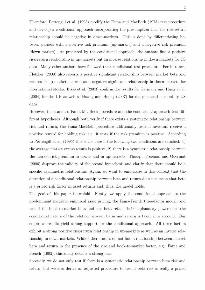
Therefore, Pettengill et al. (1995) modify the Fama and MacBeth (1973) test procedure
and develop a conditional approach incorporating the presumption that the risk-return
relationship should be negative in down-markets. This is done by differentiating be-
tween periods with a positive risk premium (up-market) and a negative risk premium
(down-market). As predicted by the conditional approach, the authors find a positive
risk-return relationship in up-markets but an inverse relationship in down-markets for US
data. Many other authors have followed their conditional test procedure. For instance,
Fletcher (2000) also reports a positive significant relationship between market beta and
returns in up-markets as well as a negative significant relationship in down-markets for
international stocks. Elsas et al. (2003) confirm the results for Germany and Hung et al.
(2004) for the UK as well as Huang and Hueng (2007) for daily instead of monthly US
data.
However, the standard Fama-MacBeth procedure and the conditional approach test dif-
ferent hypotheses. Although both verify if there exists a systematic relationship between
risk and return, the Fama-MacBeth procedure additionally tests if investors receive a
positive reward for holding risk, i.e. it tests if the risk premium is positive. According
to Pettengill et al. (1995) this is the case if the following two conditions are satisfied: 1)
the average market excess return is positive, 2) there is a symmetric relationship between
the market risk premium in down- and in up-markets. Though, Freeman and Guermat
(2006) disprove the validity of the second hypothesis and clarify that there should be a
specific asymmetric relationship. Again, we want to emphasize in this context that the
detection of a conditional relationship between beta and return does not mean that beta
is a priced risk factor in asset returns and, thus, the model holds.
The goal of this paper is twofold. Firstly, we apply the conditional approach to the
predominant model in empirical asset pricing, the Fama-French three-factor model, and
test if the book-to-market beta and size beta retain their explanatory power once the
conditional nature of the relation between betas and return is taken into account. Our
empirical results yield strong support for the conditional approach. All three factors
exhibit a strong positive risk-return relationship in up-markets as well as an inverse rela-
tionship in down-markets. While other studies do not find a relationship between market
beta and return in the presence of the size and book-to-market factor, e.g. Fama and
French (1992), this study detects a strong one.
Secondly, we do not only test if there is a systematic relationship between beta risk and
return, but we also derive an adjusted procedure to test if beta risk is really a priced
3
factor within the conditional approach. Our adjusted procedure automatically tests ei-
ther hypotheses. Thus, it enables us to compare the standard Fama-MacBeth test with
the conditional test procedure and to shed some light on previous studies dealing with
the conditional approach. Our derivation of the adjusted conditional test extends the
test of Freeman and Guermat (2006) to multifactor models. Within the framework of
the CAPM Freeman and Guermat show that the adjusted conditional test has a power
similar to that of the standard Fama-MacBeth test under the assumption of normally
distributed returns. However, they conjecture that the conditional test is more powerful
when applied to empirical data because of the unconditional leptokurtosis in observed
stock returns. In order to evaluate their conjecture, we use empirical stock market data
rather than simulations. Furthermore, in constrast to most of the existing literature on
the conditional relationship between risk factors and returns, we allow for time-variant
betas. Our results illustrate that the market beta is not a priced factor, whereas the size
and book-to-market beta are priced. Those results are qualitatively identical to those from
the standard Fama-MacBeth test and hence, our study supports the results in Freeman
and Guermat (2006). Contrariwise, our results conflict with other studies, e.g. Pettengill
et al. (1995), basing their test on the above mentioned hypothesis that there is a symmet-
ric relationship between the expected market excess return in down- and in up-markets.1
The remainder of the paper is organized as follows. In the next section we introduce
the conditional approach in the setting of the Fama-French three-factor model and the
econometric methodology. Section 3 discusses the data and the construction of the size
and book-to-market factor. Section 4 reports the empirical results of the standard Fama-
MacBeth and the conditional test. Subsequently, we present the derivation of the adjusted
conditional test as well as its empirical results. Section 6 concludes.
2 Methodology
We consider the Fama-French three-factor model and, in contrast to most of the existing
literature, allow for time-varying betas. The decision to allow the sensitivities to the risk
factors to change over time is made in view of the several decades long data set used
and the apparent change in asset and portfolio betas over time that is found in the data.
The relevance of time-varying betas is emphasized in several papers, e.g. Harvey (1989),
Ferson and Harvey (1991, 1993) as well as Jagannathan and Wang (1996). The three risk1We wish to emphasize that we do not remove all problems associated with empirical tests of asset
pricing models like e.g. the unobservability of the market portfolio as mentioned by Roll (1977).
4
factors of the Fama-French model are denoted by m for market risk, smb for the size risk
factor (’small minus big’) relating to the market value of equity, and hml for the book-
to-market factor (’high minus low’). Thus, the sensitivities of a portfolio i to the risk
factors at time t are denoted βmi,t, β
smbi,t , βhml
i,t . Our empirical validations are based on the
Fama-MacBeth (1973) approach, which is widely used in empirical asset pricing. Besides
the advantage of an easy implementation it automatically corrects standard deviations
for heteroscedasticity, which is a widespread problem among asset returns. We estimate
the Fama-French betas for every portfolio from the following time-series regression,
rei,t = αi,t + βm
i,trem,t + βsmb
i,t rsmb,t + βhmli,t rhml,t + εi,t (1)
where rei,t denotes the excess return of asset i, re
m,t its market excess return, rsmb,t and
rhml,t its returns on the smb and hml portfolios, respectively. This procedure is repeated
by rolling the window of 60 months of observations one month ahead. Rolling windows
of five years make an appropriate compromise between adjusting to the latest changes
and avoiding of noise in the monthly estimations. The rolling five year windows have
also been suggested in earlier literature such as Groenewold and Fraser (1997) and Fraser
et al. (2004). The next step consists in estimating the risk premia λ0,t, λm,t, λsmb,t and
λhml,t using the estimated betas β̂mi,t, β̂smb
i,t and β̂hmli,t from equation 1 , i.e. computing
cross-sectional regressions for every month,
rei,t = λ0,t + λm,tβ̂
mi,t + λsmb,tβ̂
smbi,t + λhml,tβ̂
hmli,t + ηi,t (2)
The λj,t’s, j = 0,m, smb, hml, are the risk premia which offset the investors for the risk
taken. The coefficient λ0,t is interpreted as the expected return of a zero beta portfolio,
λm,t as the market price of risk, λsmb,t and λhml,t as the price of risk stemming from the
size and the book-to-market value of the firm.2 Since the betas are estimated from a
first-step regression, standard errors for the second regression can be misleading. In order
to circumvent the presence of this errors-in-variables problem we apply a correction to
the standard errors as proposed by Shanken (1992). Even though, the Shanken correction
has to be treated critically because in practical applications it often yields a modified
cross-product of the estimated beta vectors that is not positive definite as it should be.3
2The interpretation of the size and book-to-market risk is discussed in the literature. For instance,according to Amihud and Mendelson (1986, 1991) size may proxy for liquidity risk and Vassalou andXing (2004) argue that the book-to-market ratio captures default risk.
3See Shanken and Weinstein (2006).
5
Estimating equation 2 by the Fama-MacBeth procedure leads to conclusions on whether
the risk factors are priced. For instance, if λm,t is nonzero, market risk is a priced factor.
If, on the other hand, λm,t is not distinguishable from zero, then market risk is not priced.
This can be the case either if there does not exist a relationship between beta and return
or if it does exist but the market risk premium is not distinguishable from zero. Therefore,
it is possible that beta is not priced despite the existence of a risk-return relationship. On
this account we apply a procedure suggested by Pettengill et al. (1995), which exclusively
tests the relationship between beta and realized returns conditional on whether the market
excess return, i.e. the realized market risk premium, is positive or negative. This test
takes into account that empirical tests are based on realized returns although the CAPM
is stated in expectational terms. According to the CAPM the expected risk premium is
always positive4 and, thus, there should exist a positive risk-return relation. However, the
realized risk premium can also be negative implying a negative relation between beta and
return. In order to test the systematic relationship between risk and return the following
equation is estimated:
rei,t = λ0,t + λ+
m,tδtβ̂mi,t + λ−m,t(1− δt)β̂m
i,t + ηi,t (3)
While Pettengill et al. conduct this procedure for the CAPM and for beta constant over
time, we apply the Fama-French three-factor model and allow for time-varying betas.
That is, we estimate the following equation.
rei,t = λ0,t + λ+
m,tδ1,tβ̂mi,t + λ−m,t(1− δ1,t)β̂
mi,t
+ λ+smb,tδ2,tβ̂
smbi,t + λ−smb,t(1− δ2,t)β̂
smbi,t + λ+
hml,tδ3,tβ̂hmli,t + λ−hml,t(1− δ3,t)β̂
hmli,t + ηi,t
(4)
The δ’s are dummy variables with the value 1 if the market, the smb and the hml portfo-
lios, respectively, yield a positive excess return and 0 otherwise. This means we conduct
separate regressions for up- and down-periods of the three risk factors for every month.
Afterwards, the parameters are averaged to obtain estimates for the risk premia.
While the Fama-MacBeth procedure tests whether betas are priced risk factors, the con-
ditional approach as applied here only enables us to test whether there is a systematic
relation between a risk factor and the realized returns. In other words, finding a signifi-
cant relation between beta risk and return does not automatically imply that beta risk is
priced and the model holds.4This follows from the assumption that agents are risk averse and that there is a positive net supply
of market risk.
6
3 Data
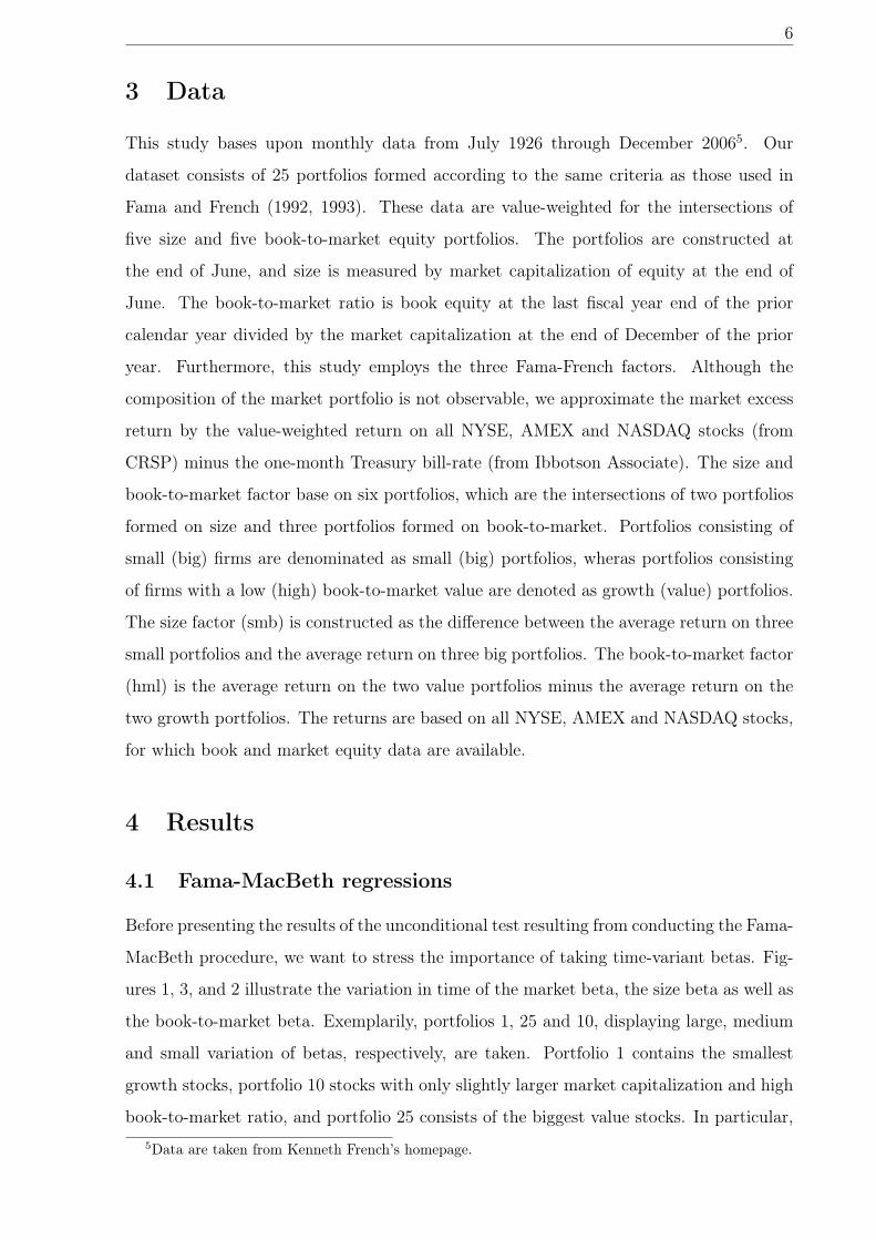
This study bases upon monthly data from July 1926 through December 20065. Our
dataset consists of 25 portfolios formed according to the same criteria as those used in
Fama and French (1992, 1993). These data are value-weighted for the intersections of
five size and five book-to-market equity portfolios. The portfolios are constructed at
the end of June, and size is measured by market capitalization of equity at the end of
June. The book-to-market ratio is book equity at the last fiscal year end of the prior
calendar year divided by the market capitalization at the end of December of the prior
year. Furthermore, this study employs the three Fama-French factors. Although the
composition of the market portfolio is not observable, we approximate the market excess
return by the value-weighted return on all NYSE, AMEX and NASDAQ stocks (from
CRSP) minus the one-month Treasury bill-rate (from Ibbotson Associate). The size and
book-to-market factor base on six portfolios, which are the intersections of two portfolios
formed on size and three portfolios formed on book-to-market. Portfolios consisting of
small (big) firms are denominated as small (big) portfolios, wheras portfolios consisting
of firms with a low (high) book-to-market value are denoted as growth (value) portfolios.
The size factor (smb) is constructed as the difference between the average return on three
small portfolios and the average return on three big portfolios. The book-to-market factor
(hml) is the average return on the two value portfolios minus the average return on the
two growth portfolios. The returns are based on all NYSE, AMEX and NASDAQ stocks,
for which book and market equity data are available.
4 Results
4.1 Fama-MacBeth regressions
Before presenting the results of the unconditional test resulting from conducting the Fama-
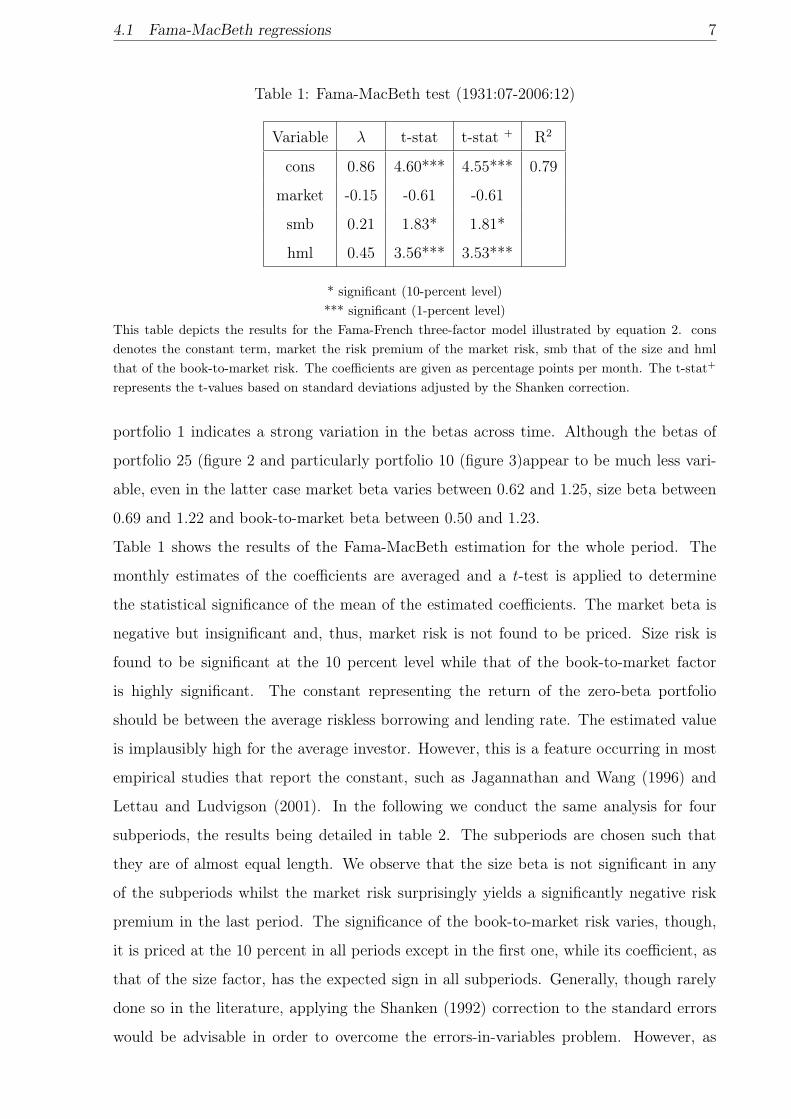
MacBeth procedure, we want to stress the importance of taking time-variant betas. Fig-
ures 1, 3, and 2 illustrate the variation in time of the market beta, the size beta as well as
the book-to-market beta. Exemplarily, portfolios 1, 25 and 10, displaying large, medium
and small variation of betas, respectively, are taken. Portfolio 1 contains the smallest
growth stocks, portfolio 10 stocks with only slightly larger market capitalization and high
book-to-market ratio, and portfolio 25 consists of the biggest value stocks. In particular,5Data are taken from Kenneth French’s homepage.
4.1 Fama-MacBeth regressions 7
Table 1: Fama-MacBeth test (1931:07-2006:12)
Variable λ t-stat t-stat + R2
cons 0.86 4.60*** 4.55*** 0.79
market -0.15 -0.61 -0.61
smb 0.21 1.83* 1.81*
hml 0.45 3.56*** 3.53***
* significant (10-percent level)*** significant (1-percent level)
This table depicts the results for the Fama-French three-factor model illustrated by equation 2. consdenotes the constant term, market the risk premium of the market risk, smb that of the size and hmlthat of the book-to-market risk. The coefficients are given as percentage points per month. The t-stat+
represents the t-values based on standard deviations adjusted by the Shanken correction.
portfolio 1 indicates a strong variation in the betas across time. Although the betas of
portfolio 25 (figure 2 and particularly portfolio 10 (figure 3)appear to be much less vari-
able, even in the latter case market beta varies between 0.62 and 1.25, size beta between
0.69 and 1.22 and book-to-market beta between 0.50 and 1.23.
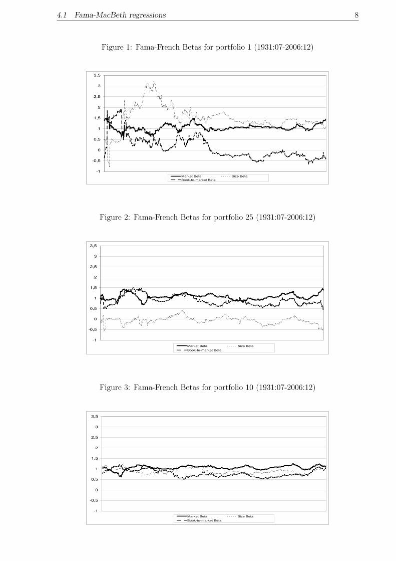
Table 1 shows the results of the Fama-MacBeth estimation for the whole period. The
monthly estimates of the coefficients are averaged and a t-test is applied to determine
the statistical significance of the mean of the estimated coefficients. The market beta is
negative but insignificant and, thus, market risk is not found to be priced. Size risk is
found to be significant at the 10 percent level while that of the book-to-market factor
is highly significant. The constant representing the return of the zero-beta portfolio
should be between the average riskless borrowing and lending rate. The estimated value
is implausibly high for the average investor. However, this is a feature occurring in most
empirical studies that report the constant, such as Jagannathan and Wang (1996) and
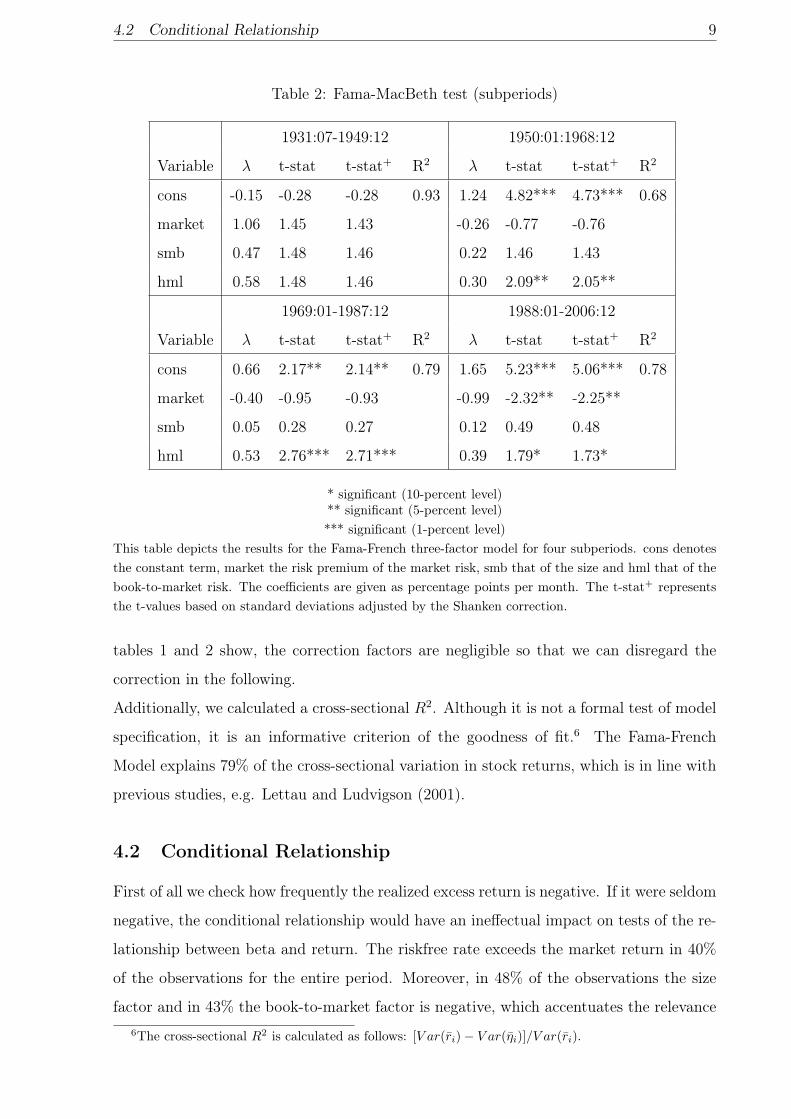
Lettau and Ludvigson (2001). In the following we conduct the same analysis for four
subperiods, the results being detailed in table 2. The subperiods are chosen such that
they are of almost equal length. We observe that the size beta is not significant in any
of the subperiods whilst the market risk surprisingly yields a significantly negative risk
premium in the last period. The significance of the book-to-market risk varies, though,
it is priced at the 10 percent in all periods except in the first one, while its coefficient, as
that of the size factor, has the expected sign in all subperiods. Generally, though rarely
done so in the literature, applying the Shanken (1992) correction to the standard errors
would be advisable in order to overcome the errors-in-variables problem. However, as
4.1 Fama-MacBeth regressions 8
Figure 1: Fama-French Betas for portfolio 1 (1931:07-2006:12)
-1
-0,5
0
0,5
1
1,5
2
2,5
3
3,5
Market Beta Size Beta
Book-to-market Beta
Figure 2: Fama-French Betas for portfolio 25 (1931:07-2006:12)
-1
-0,5
0
0,5
1
1,5
2
2,5
3
3,5
Market Beta Size Beta
Book-to-market Beta
Figure 3: Fama-French Betas for portfolio 10 (1931:07-2006:12)
-1
-0,5
0
0,5
1
1,5
2
2,5
3
3,5
Market Beta Size Beta
Book-to-market Beta
4.2 Conditional Relationship 9
Table 2: Fama-MacBeth test (subperiods)
1931:07-1949:12 1950:01:1968:12
Variable λ t-stat t-stat+ R2 λ t-stat t-stat+ R2
cons -0.15 -0.28 -0.28 0.93 1.24 4.82*** 4.73*** 0.68
market 1.06 1.45 1.43 -0.26 -0.77 -0.76
smb 0.47 1.48 1.46 0.22 1.46 1.43
hml 0.58 1.48 1.46 0.30 2.09** 2.05**
1969:01-1987:12 1988:01-2006:12
Variable λ t-stat t-stat+ R2 λ t-stat t-stat+ R2
cons 0.66 2.17** 2.14** 0.79 1.65 5.23*** 5.06*** 0.78
market -0.40 -0.95 -0.93 -0.99 -2.32** -2.25**
smb 0.05 0.28 0.27 0.12 0.49 0.48
hml 0.53 2.76*** 2.71*** 0.39 1.79* 1.73*
* significant (10-percent level)** significant (5-percent level)*** significant (1-percent level)
This table depicts the results for the Fama-French three-factor model for four subperiods. cons denotesthe constant term, market the risk premium of the market risk, smb that of the size and hml that of thebook-to-market risk. The coefficients are given as percentage points per month. The t-stat+ representsthe t-values based on standard deviations adjusted by the Shanken correction.
tables 1 and 2 show, the correction factors are negligible so that we can disregard the
correction in the following.
Additionally, we calculated a cross-sectional R2. Although it is not a formal test of model
specification, it is an informative criterion of the goodness of fit.6 The Fama-French
Model explains 79% of the cross-sectional variation in stock returns, which is in line with
previous studies, e.g. Lettau and Ludvigson (2001).
4.2 Conditional Relationship
First of all we check how frequently the realized excess return is negative. If it were seldom
negative, the conditional relationship would have an ineffectual impact on tests of the re-
lationship between beta and return. The riskfree rate exceeds the market return in 40%
of the observations for the entire period. Moreover, in 48% of the observations the size
factor and in 43% the book-to-market factor is negative, which accentuates the relevance6The cross-sectional R2 is calculated as follows: [V ar(r̄i)− V ar(η̄i)]/V ar(r̄i).
4.2 Conditional Relationship 10
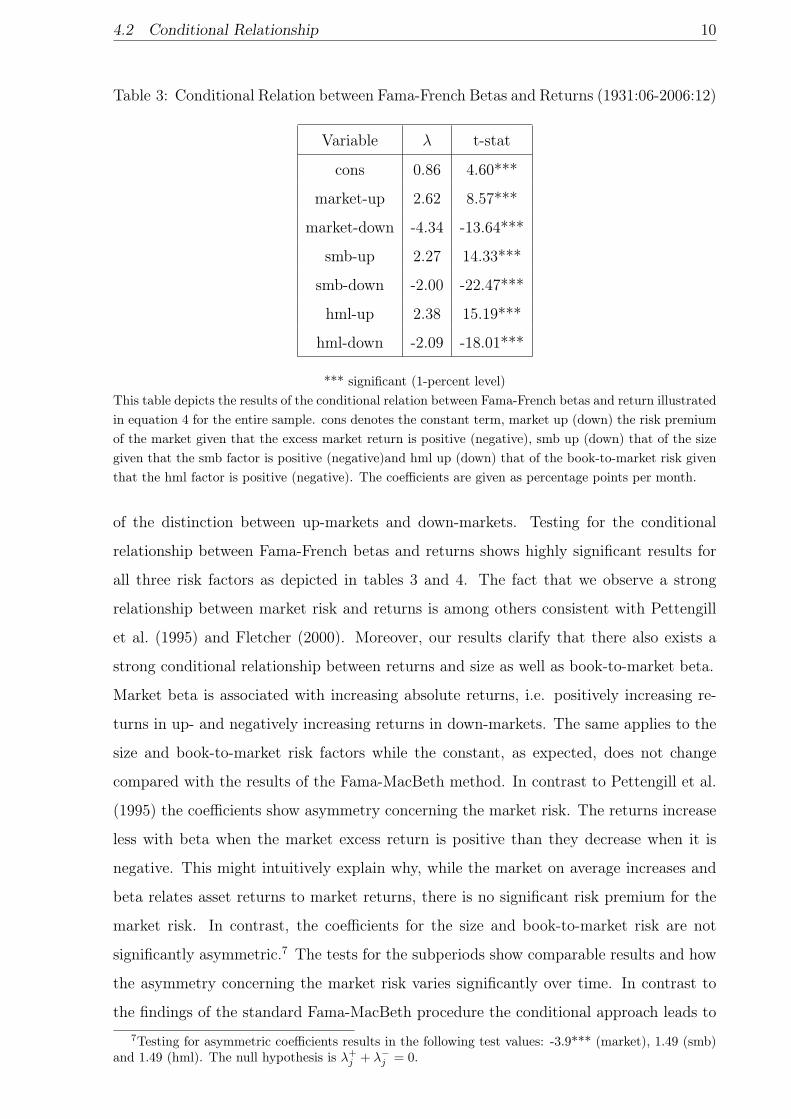
Table 3: Conditional Relation between Fama-French Betas and Returns (1931:06-2006:12)
Variable λ t-stat
cons 0.86 4.60***
market-up 2.62 8.57***
market-down -4.34 -13.64***
smb-up 2.27 14.33***
smb-down -2.00 -22.47***
hml-up 2.38 15.19***
hml-down -2.09 -18.01***
*** significant (1-percent level)This table depicts the results of the conditional relation between Fama-French betas and return illustratedin equation 4 for the entire sample. cons denotes the constant term, market up (down) the risk premiumof the market given that the excess market return is positive (negative), smb up (down) that of the sizegiven that the smb factor is positive (negative)and hml up (down) that of the book-to-market risk giventhat the hml factor is positive (negative). The coefficients are given as percentage points per month.
of the distinction between up-markets and down-markets. Testing for the conditional
relationship between Fama-French betas and returns shows highly significant results for
all three risk factors as depicted in tables 3 and 4. The fact that we observe a strong
relationship between market risk and returns is among others consistent with Pettengill
et al. (1995) and Fletcher (2000). Moreover, our results clarify that there also exists a
strong conditional relationship between returns and size as well as book-to-market beta.
Market beta is associated with increasing absolute returns, i.e. positively increasing re-
turns in up- and negatively increasing returns in down-markets. The same applies to the
size and book-to-market risk factors while the constant, as expected, does not change
compared with the results of the Fama-MacBeth method. In contrast to Pettengill et al.
(1995) the coefficients show asymmetry concerning the market risk. The returns increase
less with beta when the market excess return is positive than they decrease when it is
negative. This might intuitively explain why, while the market on average increases and
beta relates asset returns to market returns, there is no significant risk premium for the
market risk. In contrast, the coefficients for the size and book-to-market risk are not
significantly asymmetric.7 The tests for the subperiods show comparable results and how
the asymmetry concerning the market risk varies significantly over time. In contrast to
the findings of the standard Fama-MacBeth procedure the conditional approach leads to7Testing for asymmetric coefficients results in the following test values: -3.9*** (market), 1.49 (smb)
and 1.49 (hml). The null hypothesis is λ+j + λ−j = 0.
11
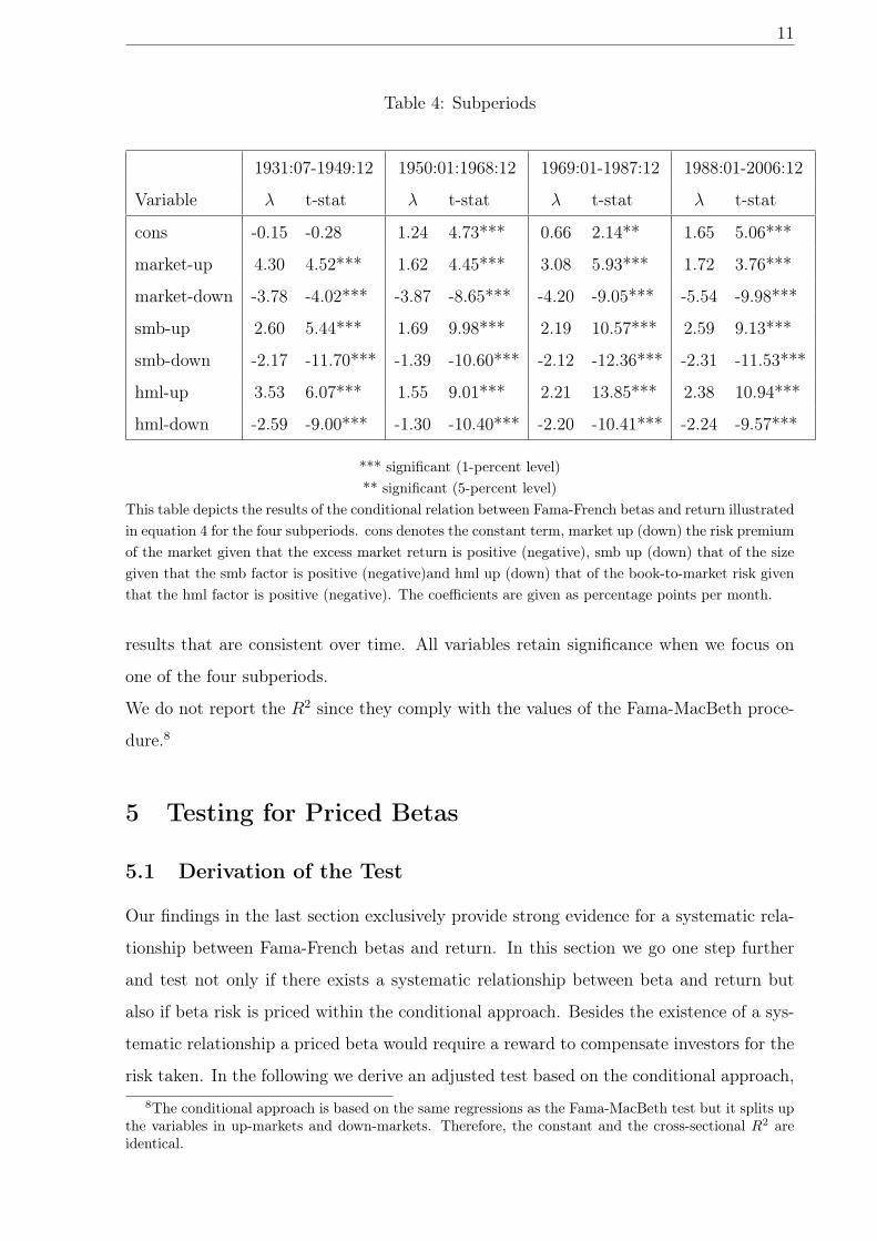
Table 4: Subperiods
1931:07-1949:12 1950:01:1968:12 1969:01-1987:12 1988:01-2006:12
Variable λ t-stat λ t-stat λ t-stat λ t-stat
cons -0.15 -0.28 1.24 4.73*** 0.66 2.14** 1.65 5.06***
market-up 4.30 4.52*** 1.62 4.45*** 3.08 5.93*** 1.72 3.76***
market-down -3.78 -4.02*** -3.87 -8.65*** -4.20 -9.05*** -5.54 -9.98***
smb-up 2.60 5.44*** 1.69 9.98*** 2.19 10.57*** 2.59 9.13***
smb-down -2.17 -11.70*** -1.39 -10.60*** -2.12 -12.36*** -2.31 -11.53***
hml-up 3.53 6.07*** 1.55 9.01*** 2.21 13.85*** 2.38 10.94***
hml-down -2.59 -9.00*** -1.30 -10.40*** -2.20 -10.41*** -2.24 -9.57***
*** significant (1-percent level)** significant (5-percent level)
This table depicts the results of the conditional relation between Fama-French betas and return illustratedin equation 4 for the four subperiods. cons denotes the constant term, market up (down) the risk premiumof the market given that the excess market return is positive (negative), smb up (down) that of the sizegiven that the smb factor is positive (negative)and hml up (down) that of the book-to-market risk giventhat the hml factor is positive (negative). The coefficients are given as percentage points per month.
results that are consistent over time. All variables retain significance when we focus on
one of the four subperiods.
We do not report the R2 since they comply with the values of the Fama-MacBeth proce-
dure.8
5 Testing for Priced Betas
5.1 Derivation of the Test
Our findings in the last section exclusively provide strong evidence for a systematic rela-
tionship between Fama-French betas and return. In this section we go one step further
and test not only if there exists a systematic relationship between beta and return but
also if beta risk is priced within the conditional approach. Besides the existence of a sys-
tematic relationship a priced beta would require a reward to compensate investors for the
risk taken. In the following we derive an adjusted test based on the conditional approach,8The conditional approach is based on the same regressions as the Fama-MacBeth test but it splits up
the variables in up-markets and down-markets. Therefore, the constant and the cross-sectional R2 areidentical.
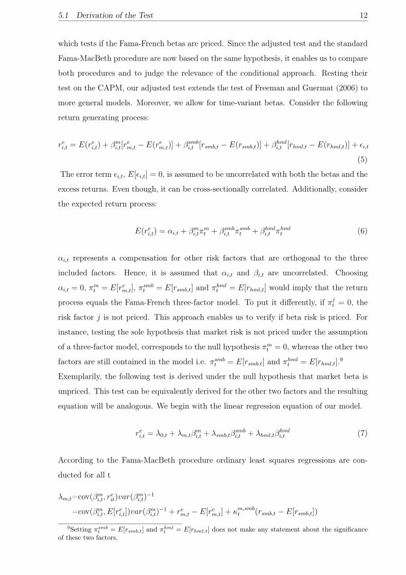
5.1 Derivation of the Test 12
which tests if the Fama-French betas are priced. Since the adjusted test and the standard
Fama-MacBeth procedure are now based on the same hypothesis, it enables us to compare
both procedures and to judge the relevance of the conditional approach. Resting their
test on the CAPM, our adjusted test extends the test of Freeman and Guermat (2006) to
more general models. Moreover, we allow for time-variant betas. Consider the following
return generating process:
rei,t = E(re
i,t) + βmi,t[r
em,t − E(re
m,t)] + βsmbi,t [rsmb,t − E(rsmb,t)] + βhml
i,t [rhml,t − E(rhml,t)] + εi,t
(5)
The error term εi,t, E[εi,t] = 0, is assumed to be uncorrelated with both the betas and the
excess returns. Even though, it can be cross-sectionally correlated. Additionally, consider
the expected return process:
E(rei,t) = αi,t + βm
i,tπmt + βsmb
i,t πsmbt + βhml
i,t πhmlt (6)
αi,t represents a compensation for other risk factors that are orthogonal to the three
included factors. Hence, it is assumed that αi,t and βi,t are uncorrelated. Choosing
αi,t = 0, πmt = E[re
m,t], πsmbt = E[rsmb,t] and πhml
t = E[rhml,t] would imply that the return
process equals the Fama-French three-factor model. To put it differently, if πjt = 0, the
risk factor j is not priced. This approach enables us to verify if beta risk is priced. For
instance, testing the sole hypothesis that market risk is not priced under the assumption
of a three-factor model, corresponds to the null hypothesis πmt = 0, whereas the other two
factors are still contained in the model i.e. πsmbt = E[rsmb,t] and πhml
t = E[rhml,t].9
Exemplarily, the following test is derived under the null hypothesis that market beta is
unpriced. This test can be equivalently derived for the other two factors and the resulting
equation will be analogous. We begin with the linear regression equation of our model.
rei,t = λ0,t + λm,tβ
mi,t + λsmb,tβ
smbi,t + λhml,tβ
hmli,t (7)
According to the Fama-MacBeth procedure ordinary least squares regressions are con-
ducted for all t
λm,t=cov(βmi,t, r
eit)var(β
mi,t)−1
=cov(βmi,t, E[re
i,t])var(βmi,t)−1 + re
m,t − E[rem,t] + κm,smb
t (rsmb,t − E[rsmb,t])
9Setting πsmbt = E[rsmb,t] and πhml
t = E[rhml,t] does not make any statement about the significanceof these two factors.
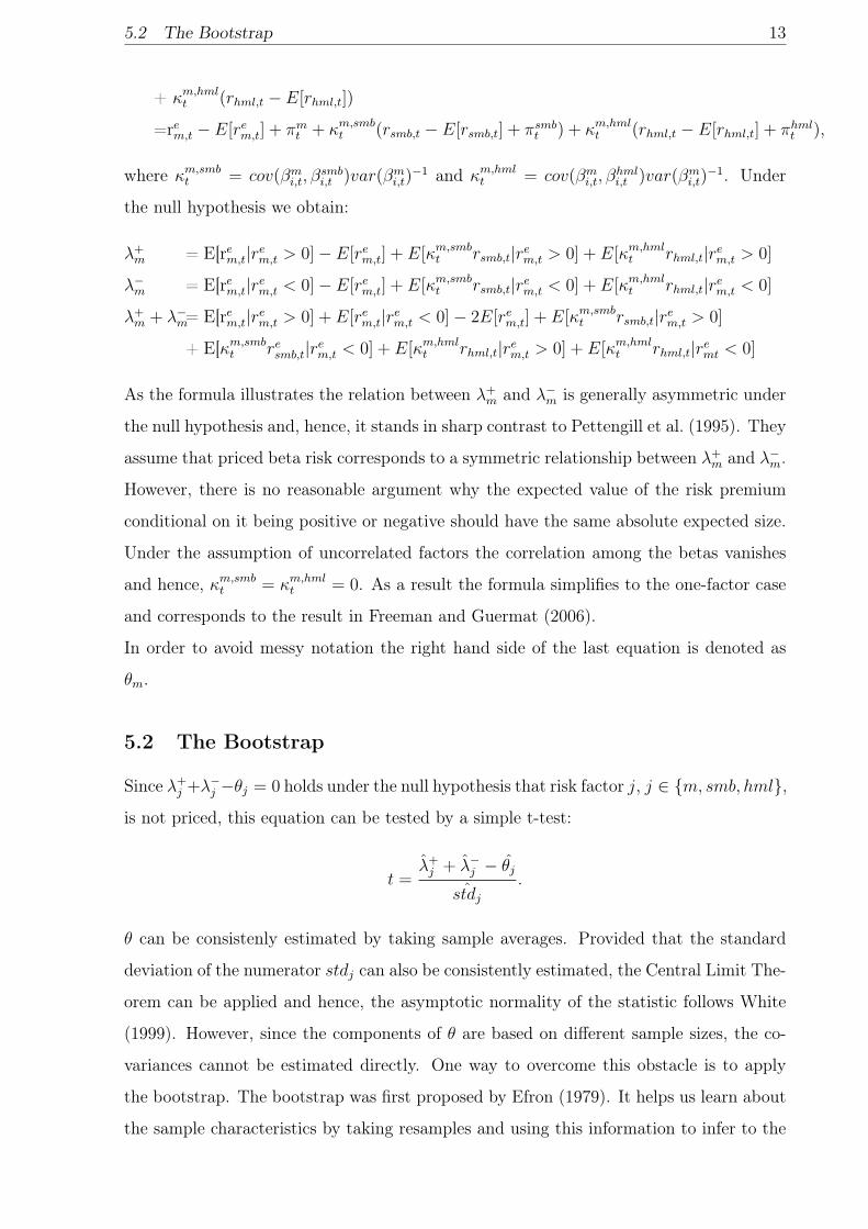
5.2 The Bootstrap 13
+ κm,hmlt (rhml,t − E[rhml,t])
=rem,t − E[rem,t] + πm
t + κm,smbt (rsmb,t − E[rsmb,t] + πsmb
t ) + κm,hmlt (rhml,t − E[rhml,t] + πhml
t ),
where κm,smbt = cov(βm
i,t, βsmbi,t )var(βm
i,t)−1 and κm,hml
t = cov(βmi,t, β
hmli,t )var(βm
i,t)−1. Under
the null hypothesis we obtain:
λ+m = E[rem,t|re
m,t > 0]− E[rem,t] + E[κm,smb
t rsmb,t|rem,t > 0] + E[κm,hml
t rhml,t|rem,t > 0]
λ−m = E[rem,t|rem,t < 0]− E[re
m,t] + E[κm,smbt rsmb,t|re
m,t < 0] + E[κm,hmlt rhml,t|re
m,t < 0]
λ+m + λ−m= E[rem,t|re
m,t > 0] + E[rem,t|re
m,t < 0]− 2E[rem,t] + E[κm,smb
t rsmb,t|rem,t > 0]
+ E[κm,smbt re
smb,t|rem,t < 0] + E[κm,hml
t rhml,t|rem,t > 0] + E[κm,hml
t rhml,t|remt < 0]
As the formula illustrates the relation between λ+m and λ−m is generally asymmetric under
the null hypothesis and, hence, it stands in sharp contrast to Pettengill et al. (1995). They
assume that priced beta risk corresponds to a symmetric relationship between λ+m and λ−m.
However, there is no reasonable argument why the expected value of the risk premium
conditional on it being positive or negative should have the same absolute expected size.
Under the assumption of uncorrelated factors the correlation among the betas vanishes
and hence, κm,smbt = κm,hml
t = 0. As a result the formula simplifies to the one-factor case
and corresponds to the result in Freeman and Guermat (2006).
In order to avoid messy notation the right hand side of the last equation is denoted as
θm.
5.2 The Bootstrap
Since λ+j +λ−j −θj = 0 holds under the null hypothesis that risk factor j, j ∈ {m, smb, hml},
is not priced, this equation can be tested by a simple t-test:
t =λ̂+
j + λ̂−j − θ̂j
ˆstdj
.
θ can be consistenly estimated by taking sample averages. Provided that the standard
deviation of the numerator stdj can also be consistently estimated, the Central Limit The-
orem can be applied and hence, the asymptotic normality of the statistic follows White
(1999). However, since the components of θ are based on different sample sizes, the co-
variances cannot be estimated directly. One way to overcome this obstacle is to apply
the bootstrap. The bootstrap was first proposed by Efron (1979). It helps us learn about
the sample characteristics by taking resamples and using this information to infer to the
5.3 Empirical Results 14
population. As shown by Babu and Singh (1984) the bootstrap can be used to consis-
tently estimate a wide range of statistics, including not only the sample mean but also the
sample variance and smooth transforms of these statistics. In our setting the bootstrap
is applied as follows. T observations are independently drawn from the four variables
rej,t, λj, rk,tκ
j,kt and rl,tκ
j,lt with replacement where k, l denote the two risk factors different
from j. This gives us a new sample (rej,t∗, λ∗j , (rk,tκ
j,kt )∗, (rl,tκ
j,lt )∗). By calculating λ̂+
j∗,
λ̂−j∗ and θ̂∗ from the new sample, we obtain an estimate for the numerator. This result
is saved and the whole procedure is repeated S times. Finally, the bootstrap variance is
the sample variance of the S estimates of the numerator. In order to choose S sufficiently
large, we take S equal to 10000.
However, this procedure relies on the assumption that returns are identically and inde-
pendently distributed. In order to account for possible autocorrelation and clusterings
we conduct the block bootstrap additionally. The Moving Block Bootstrap developed by
Künsch (1989) draws blocks of length l instead of drawing T observations independently.
Since the validity of the block bootstrap requires limT→∞l2
T= 0, we choose l = T
13 . Lahiri
(1999) shows that the Moving block Bootstrap performs better than other block boot-
straps in terms of the mean squared error. With repect to this criterion, Künsch (1989)
determine that l = T13 is the optimal order of the block length.
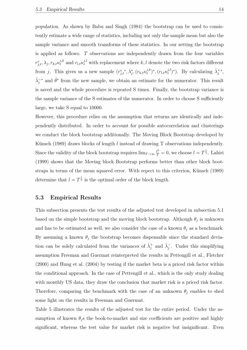
5.3 Empirical Results
This subsection presents the test results of the adjusted test developed in subsection 5.1
based on the simple bootstrap and the moving block bootstrap. Although θj is unknown
and has to be estimated as well, we also consider the case of a known θj as a benchmark.
By assuming a known θj the bootstrap becomes dispensable since the standard devia-
tion can be solely calculated from the variances of λ̂+j and λ̂−j . Under this simplifying
assumption Freeman and Guermat reinterpreted the results in Pettengill et al., Fletcher
(2000) and Hung et al. (2004) by testing if the market beta is a priced risk factor within
the conditional approach. In the case of Pettengill et al., which is the only study dealing
with monthly US data, they draw the conclusion that market risk is a priced risk factor.
Therefore, comparing the benchmark with the case of an unknown θj enables to shed
some light on the results in Freeman and Guermat.
Table 5 illustrates the results of the adjusted test for the entire period. Under the as-
sumption of known θjs the book-to-market and size coefficients are positive and highly
significant, whereas the test value for market risk is negative but insignificant. Even
5.3 Empirical Results 15
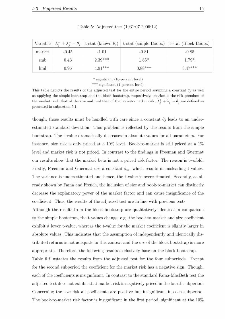
Table 5: Adjusted test (1931:07-2006:12)
Variable λ+j + λ−j − θj t-stat (known θj) t-stat (simple Boots.) t-stat (Block-Boots.)
market -0.45 -1.01 -0.81 -0.85
smb 0.43 2.39*** 1.85* 1.79*
hml 0.96 4.91*** 3.88*** 3.47***
* significant (10-percent level)*** significant (1-percent level)
This table depicts the results of the adjusted test for the entire period assuming a constant θj as wellas applying the simple bootstrap and the block bootstrap, respectively. market is the risk premium ofthe market, smb that of the size and hml that of the book-to-market risk. λ+
j + λ−j − θj are defined aspresented in subsection 5.1.
though, those results must be handled with care since a constant θj leads to an under-
estimated standard deviation. This problem is reflected by the results from the simple
bootstrap. The t-value dramatically decreases in absolute values for all parameters. For
instance, size risk is only priced at a 10% level. Book-to-market is still priced at a 1%
level and market risk is not priced. In contrast to the findings in Freeman and Guermat
our results show that the market beta is not a priced risk factor. The reason is twofold.
Firstly, Freeman and Guermat use a constant θm, which results in misleading t-values.
The variance is underestimated and hence, the t-value is overestimated. Secondly, as al-
ready shown by Fama and French, the inclusion of size and book-to-market can distinctly
decrease the explanatory power of the market factor and can cause insignficance of the
coefficient. Thus, the results of the adjusted test are in line with previous tests.
Although the results from the block bootstrap are qualitatively identical in comparison
to the simple bootstrap, the t-values change, e.g. the book-to-market and size coefficient
exhibit a lower t-value, whereas the t-value for the market coefficient is slightly larger in
absolute values. This indicates that the assumption of independently and identically dis-
tributed returns is not adequate in this context and the use of the block bootstrap is more
appropriate. Therefore, the following results exclusively base on the block bootstrap.
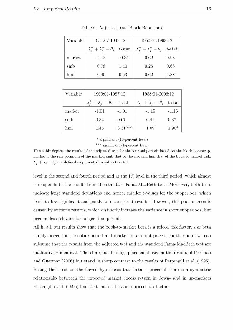
Table 6 illustrates the results from the adjusted test for the four subperiods. Except
for the second subperiod the coefficient for the market risk has a negative sign. Though,
each of the coefficients is insignificant. In contrast to the standard Fama-MacBeth test the
adjusted test does not exhibit that market risk is negatively priced in the fourth subperiod.
Concerning the size risk all coefficients are positive but insignificant in each subperiod.
The book-to-market risk factor is insignificant in the first period, significant at the 10%
5.3 Empirical Results 16
Table 6: Adjusted test (Block Bootstrap)
Variable 1931:07-1949:12 1950:01:1968:12
λ+j + λ−j − θj t-stat λ+
j + λ−j − θj t-stat
market -1.24 -0.85 0.62 0.93
smb 0.78 1.40 0.26 0.66
hml 0.40 0.53 0.62 1.88*
Variable 1969:01-1987:12 1988:01-2006:12
λ+j + λ−j − θj t-stat λ+
j + λ−j − θj t-stat
market -1.01 -1.01 -1.15 -1.16
smb 0.32 0.67 0.41 0.87
hml 1.45 3.31*** 1.09 1.90*
* significant (10-percent level)*** significant (1-percent level)
This table depicts the results of the adjusted test for the four subperiods based on the block bootstrap.market is the risk premium of the market, smb that of the size and hml that of the book-to-market risk.λ+
j + λ−j − θj are defined as presented in subsection 5.1.
level in the second and fourth period and at the 1% level in the third period, which almost
corresponds to the results from the standard Fama-MacBeth test. Moreover, both tests
indicate large standard deviations and hence, smaller t-values for the subperiods, which
leads to less significant and partly to inconsistent results. However, this phenomenon is
caused by extreme returns, which distinctly increase the variance in short subperiods, but
become less relevant for longer time periods.
All in all, our results show that the book-to-market beta is a priced risk factor, size beta
is only priced for the entire period and market beta is not priced. Furthermore, we can
subsume that the results from the adjusted test and the standard Fama-MacBeth test are
qualitatively identical. Therefore, our findings place emphasis on the results of Freeman
and Guermat (2006) but stand in sharp contrast to the results of Pettengill et al. (1995).
Basing their test on the flawed hypothesis that beta is priced if there is a symmetric
relationship betweeen the expected market excess return in down- and in up-markets
Pettengill et al. (1995) find that market beta is a priced risk factor.
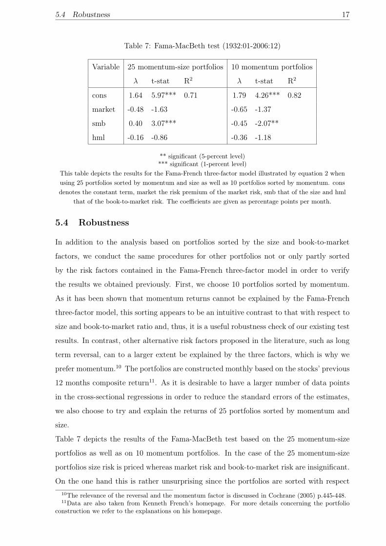
5.4 Robustness 17
Table 7: Fama-MacBeth test (1932:01-2006:12)
Variable 25 momentum-size portfolios 10 momentum portfolios
λ t-stat R2 λ t-stat R2
cons 1.64 5.97*** 0.71 1.79 4.26*** 0.82
market -0.48 -1.63 -0.65 -1.37
smb 0.40 3.07*** -0.45 -2.07**
hml -0.16 -0.86 -0.36 -1.18
** significant (5-percent level)*** significant (1-percent level)
This table depicts the results for the Fama-French three-factor model illustrated by equation 2 whenusing 25 portfolios sorted by momentum and size as well as 10 portfolios sorted by momentum. consdenotes the constant term, market the risk premium of the market risk, smb that of the size and hml
that of the book-to-market risk. The coefficients are given as percentage points per month.
5.4 Robustness
In addition to the analysis based on portfolios sorted by the size and book-to-market
factors, we conduct the same procedures for other portfolios not or only partly sorted
by the risk factors contained in the Fama-French three-factor model in order to verify
the results we obtained previously. First, we choose 10 portfolios sorted by momentum.
As it has been shown that momentum returns cannot be explained by the Fama-French
three-factor model, this sorting appears to be an intuitive contrast to that with respect to
size and book-to-market ratio and, thus, it is a useful robustness check of our existing test
results. In contrast, other alternative risk factors proposed in the literature, such as long
term reversal, can to a larger extent be explained by the three factors, which is why we
prefer momentum.10 The portfolios are constructed monthly based on the stocks’ previous
12 months composite return11. As it is desirable to have a larger number of data points
in the cross-sectional regressions in order to reduce the standard errors of the estimates,
we also choose to try and explain the returns of 25 portfolios sorted by momentum and
size.
Table 7 depicts the results of the Fama-MacBeth test based on the 25 momentum-size
portfolios as well as on 10 momentum portfolios. In the case of the 25 momentum-size
portfolios size risk is priced whereas market risk and book-to-market risk are insignificant.
On the one hand this is rather unsurprising since the portfolios are sorted with respect10The relevance of the reversal and the momentum factor is discussed in Cochrane (2005) p.445-448.11Data are also taken from Kenneth French’s homepage. For more details concerning the portfolio
construction we refer to the explanations on his homepage.
5.4 Robustness 18
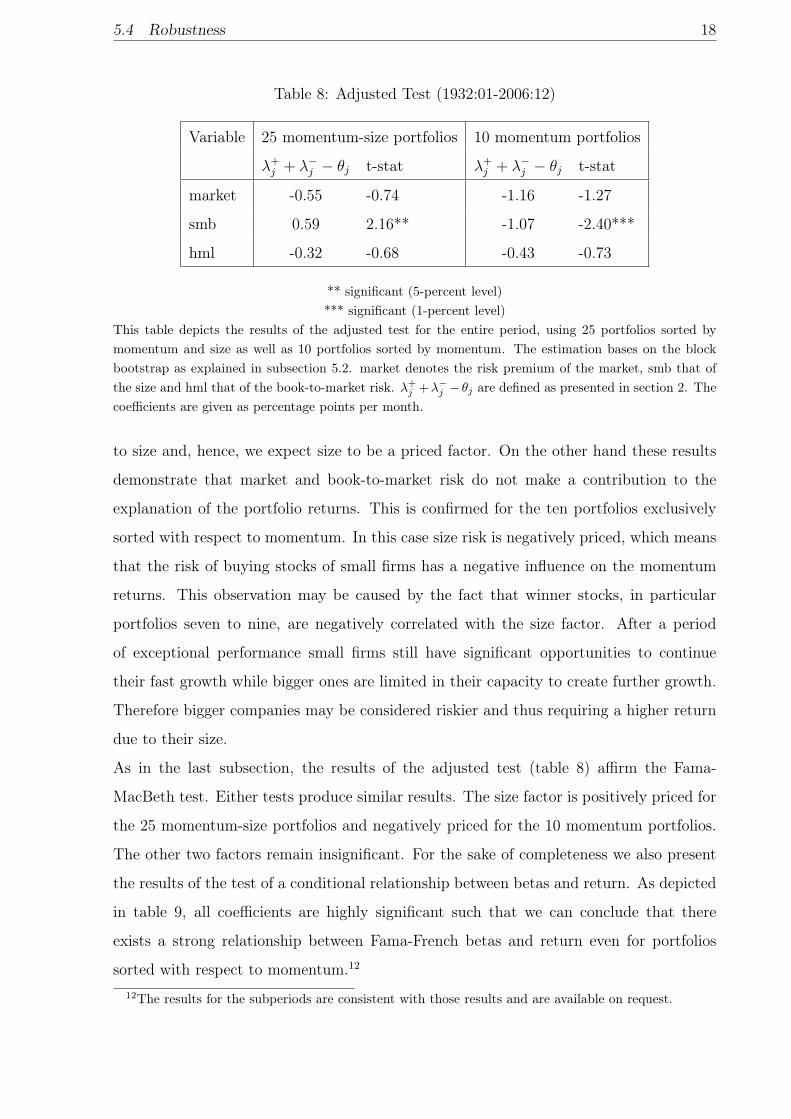
Table 8: Adjusted Test (1932:01-2006:12)
Variable 25 momentum-size portfolios 10 momentum portfolios
λ+j + λ−j − θj t-stat λ+
j + λ−j − θj t-stat
market -0.55 -0.74 -1.16 -1.27
smb 0.59 2.16** -1.07 -2.40***
hml -0.32 -0.68 -0.43 -0.73
** significant (5-percent level)*** significant (1-percent level)
This table depicts the results of the adjusted test for the entire period, using 25 portfolios sorted bymomentum and size as well as 10 portfolios sorted by momentum. The estimation bases on the blockbootstrap as explained in subsection 5.2. market denotes the risk premium of the market, smb that ofthe size and hml that of the book-to-market risk. λ+
j +λ−j − θj are defined as presented in section 2. Thecoefficients are given as percentage points per month.
to size and, hence, we expect size to be a priced factor. On the other hand these results
demonstrate that market and book-to-market risk do not make a contribution to the
explanation of the portfolio returns. This is confirmed for the ten portfolios exclusively
sorted with respect to momentum. In this case size risk is negatively priced, which means
that the risk of buying stocks of small firms has a negative influence on the momentum
returns. This observation may be caused by the fact that winner stocks, in particular
portfolios seven to nine, are negatively correlated with the size factor. After a period
of exceptional performance small firms still have significant opportunities to continue
their fast growth while bigger ones are limited in their capacity to create further growth.
Therefore bigger companies may be considered riskier and thus requiring a higher return
due to their size.
As in the last subsection, the results of the adjusted test (table 8) affirm the Fama-
MacBeth test. Either tests produce similar results. The size factor is positively priced for
the 25 momentum-size portfolios and negatively priced for the 10 momentum portfolios.
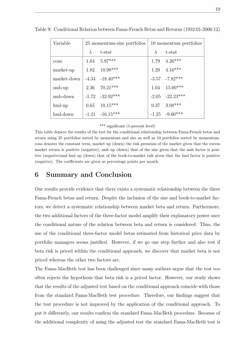
The other two factors remain insignificant. For the sake of completeness we also present
the results of the test of a conditional relationship between betas and return. As depicted
in table 9, all coefficients are highly significant such that we can conclude that there
exists a strong relationship between Fama-French betas and return even for portfolios
sorted with respect to momentum.12
12The results for the subperiods are consistent with those results and are available on request.
19
Table 9: Conditional Relation between Fama-French Betas and Returns (1932:01-2006:12)
Variable 25 momentum-size portfolios 10 momentum portfolios
λ t-stat λ t-stat
cons 1.64 5.97*** 1.79 4.26***
market-up 1.82 10.98*** 1.29 4.16***
market-down -4.34 -18.40*** -3.57 -7.82***
smb-up 2.36 70.21*** 1.04 15.00***
smb-down -1.72 -32.92*** -2.05 -22.23***
hml-up 0.65 10.15*** 0.37 3.08***
hml-down -1.21 -16.15*** -1.25 -9.60***
*** significant (1-percent level)This table depicts the results of the test for the conditional relationship between Fama-French betas andreturn using 25 portfolios sorted by momentum and size as well as 10 portfolios sorted by momentum.cons denotes the constant term, market up (down) the risk premium of the market given that the excessmarket return is positive (negative), smb up (down) that of the size given that the smb factor is posi-tive (negative)and hml up (down) that of the book-to-market risk given that the hml factor is positive(negative). The coefficients are given as percentage points per month.
6 Summary and Conclusion
Our results provide evidence that there exists a systematic relationship between the three
Fama-French betas and return. Despite the inclusion of the size and book-to-market fac-
tors, we detect a systematic relationship between market beta and return. Furthermore,
the two additional factors of the three-factor model amplify their explanatory power once
the conditional nature of the relation between beta and return is considered. Thus, the
use of the conditional three-factor model betas estimated from historical price data by
portfolio managers seems justified. However, if we go one step further and also test if
beta risk is priced within the conditional approach, we discover that market beta is not
priced whereas the other two factors are.
The Fama-MacBeth test has been challenged since many authors argue that the test too
often rejects the hypothesis that beta risk is a priced factor. However, our study shows
that the results of the adjusted test based on the conditional approach coincide with those
from the standard Fama-MacBeth test procedure. Therefore, our findings suggest that
the test procedure is not improved by the application of the conditional approach. To
put it differently, our results confirm the standard Fama-MacBeth procedure. Because of
the additional complexity of using the adjusted test the standard Fama-MacBeth test is
20
favored.
Many previous studies have applied the conditional approach as proposed by Pettengill
et al. (1995). The conditional approach takes into account that the use of realized returns
leads to a negative risk-return relationship in down-markets. Thus, from the theoretical
point of view the conditional approach is more appropriate. Even though, either previous
studies test if beta risk is priced within the framework of the conditional approach but
based on a wrong hypothesis (symmetry of the λ coefficients) or they only test if there
exists a conditional relationship between beta and return. In either cases the results of
the test cannot be related to the results from the standard Fama-MacBeth procedure. In
this paper we make these tests comparable by using the conditional approach to derive an
adjusted test for priced beta and detect that the results are qualitatively identical using
different data sets and checking four subperiods. Our results confirm those in Freeman
and Guermat (2006). They show that either tests have a similar power in the special case
of normally distributed returns.
We do not conclude that the conditional approach is irrelevant but we want to point out
that the choice of the test procedure depends on the research question. Testing for priced
beta risk does not make the conditional approach necessary. Nevertheless, if we only fo-
cus on testing for a systematic relationship between risk and return, then the conditional
approach is suitable.
REFERENCES 21
References
Amihud, Y. and H. Mendelson (1986). Asset pricing and the bid-ask spread. Journal of
Financial Economics 17, 223–249.
Amihud, Y. and H. Mendelson (1991). Liquidity and asset prices. Finanzmarkt und
Portfolio Management 3, 235–240.
Babu, G. J. and K. Singh (1984). On one term edgeworth correction by efron’s boostrap.
Sankhya: The Indian Journal of Statistics 46 (A), 219–232.
Banz, R. W. (1981). The relationship between return and market value of common stocks.
Journal of Financial Economics 9, 3–18.
Black, F., M. Jensen, and M. Scholes (1972). Studies in the Theory of Capital Markets,
Chapter The Capital asset pricing model: some empirical tests, pp. 79–121. Praeger,
New York.
Cochrane, J. (2005). Asset Pricing (revised ed.). Princeton University Press.
Efron, B. (1979). Bootstrap methods: Another look at the jackknife. Annals of Statis-
tics 7, 1.26.
Elsas, R., M. El-Shaer, and E. Theissen (2003). Beta and returns revisited: Evidence from
the german stock market. International Financial Markets, Institutions & Money 13,
1–18.
Fama, E. F. and K. R. French (1992). The cross-section of expected stock returns. Journal
of Finance 47 (2), 427–465.
Fama, E. F. and K. R. French (1993). Common risk factors in the returns on stocks and
bonds. Journal of Financial Economics 33, 3–56.
Fama, E. F. and K. R. French (1996). Multifactor explanations of asset pricing anomalies.
Journal of Finance 51 (1), 55–84.
Fama, E. F. and J. D. MacBeth (1973). Risk, return, and equilibrium: Empirical tests.
Journal of Political Economy 81 (3), 607–636.
Ferson, W. E. and C. R. Harvey (1991). The variation of economic risk premiums. Journal
of Political Economy 99, 285–315.
REFERENCES 22
Ferson, W. E. and C. R. Harvey (1993). The risk and predicitability of international
equity returns. Review of Financial Studies 6 (3), 527–566.
Fletcher, J. (2000). On the conditional relationship between beta and return in interna-
tional stock returns. International Review of Financial Analysis 9, 235–245.
Fraser, P., F. Hamelink, M. Hoesli, and B. MacGregor (2004). Time-varying beta and
the cross-sectional return-risk relation: evidence from the uk. The European Journal of
Finance 10, 255–276.
Freeman, M. C. and C. Guermat (2006). The conditional relationship between beta and
returns: A reassessment. Journal of Business Finance & Accounting 33 (7-8), 1213–
1239.
Groenewold, N. and P. Fraser (1997). Share prices and macroeconomic factors. Journal
of Business Finance & Accounting 24, 1367–1383.
Harvey, C. R. (1989). Time-varying conditional covariances in tests of asset pricing models.
Journal of Financial Economics 24, 289–317.
Huang, P. and C. J. Hueng (forthcoming). Conditional risk-return relationship in a time-
varying beta model. Quantitative Finance.
Hung, D. C.-H., M. Shackleton, and X. Xu (2004). Capm, higher co-moment and factor
models of uk stock returns. Journal of Business Finance & Accounting 31 (1-2), 87–112.
Jagannathan, R. and Z. Wang (1996). The conditional capm and the cross-section of
expected returns. Journal of Finance 51 (1).
Künsch, H. R. (1989). The jackknife and the bootstrap for general stationary observations.
The Annals of Statistics 17, 1217–1261.
Lahiri, S. N. (1999). Theoretical comparison of block bootstrap methods. The Annals of
Statistics 27, 386–404.
Lettau, M. and S. Ludvigson (2001). Resurrecting the (c)capm: A cross-sectional test
when risk premia are time-varying. Journal of Political Economy 109 (6), 1238–1287.
Lintner, J. (1965). The valuation of risk assets and the selection of risky investments in
stock portfolios and capital budgets. Review of Economics and Statistics 47 (13-37).
Mossin, J. (1966). Equilibrium in a capital asset market. Econometrica 34 (4), 768–783.
REFERENCES 23
Pettengill, G. N., S. Sundaram, and I. Mathur (1995). The conditional relation between
beta and return. Journal of Financial and Quantitative Analysis 30 (1), 101–116.
Reinganum, M. R. (1981). A new empirical perspective on the capm. Journal of Financial
and Quantitative Analysis 16 (4), 439–462.
Roll, R. (1977). A critique of the asset pricing theory’s tests: Part i: On past and potential
testability of the theory. Journal of Financial Economics 4, 129–176.
Shanken, J. (1992). On the estimation of beta-pricing models. The Review of Financial
Studies 5 (1), 1–33.
Shanken, J. and M. Weinstein (2006). Economic forces and the stock market revisited.
Journal of Empirical Finance 13, 129–144.
Sharpe, W. F. (1964). Capital asset prices: A theory of market equilibrium under condi-
tions of risk. Journal of Finance 19 (3), 425–442.
Vassalou, M. and Y. Xing (2004). Default risk and equity returns. Journal of Finance 59,
831.868.
White, H. (1999). Asymptotic Theory for Econometricias. San Diego: Academic Press.