NBER WORKING PAPER SERIES

FINANCIAL INSTABILITY, RESERVES, AND CENTRAL BANK SWAP LINESIN THE PANIC OF 2008

Maurice ObstfeldJay C. Shambaugh

Alan M. Taylor

Working Paper 14826http://www.nber.org/papers/w14826

NATIONAL BUREAU OF ECONOMIC RESEARCH1050 Massachusetts Avenue

Cambridge, MA 02138March 2009

We thank the Fondation Banque de France for supporting our research through a grant administeredby the CEPR. Matteo Maggiori provided helpful research assistance. The paper was presented at theASSA Meetings, San Francisco, January 3-5, 2009. We received many helpful comments, especiallyfrom our discussant Joshua Aizenman. All errors are ours. The views expressed herein are those ofthe author(s) and do not necessarily reflect the views of the National Bureau of Economic Research.

NBER working papers are circulated for discussion and comment purposes. They have not been peer-reviewed or been subject to the review by the NBER Board of Directors that accompanies officialNBER publications.

© 2009 by Maurice Obstfeld, Jay C. Shambaugh, and Alan M. Taylor. All rights reserved. Short sectionsof text, not to exceed two paragraphs, may be quoted without explicit permission provided that fullcredit, including © notice, is given to the source.

Financial Instability, Reserves, and Central Bank Swap Lines in the Panic of 2008Maurice Obstfeld, Jay C. Shambaugh, and Alan M. TaylorNBER Working Paper No. 14826March 2009JEL No. E42,E44,E58,F21,F31,F33,F36,F41,F42,O24

ABSTRACT

In this paper we connect the events of the last twelve months, "The Panic of 2008" as it has been called,to the demand for international reserves. In previous work, we have shown that international reservedemand can be rationalized by a central bank’s desire to backstop the broad money supply to avertthe possibility of an internal/external double drain (a bank run combined with capital flight). Thus,simply looking at trade or short-term debt as motivations for reserve holdings is insufficient; one mustalso consider the size of the banking system (M2). Here, we show that a country’s reserve holdingsjust before the current crisis, relative to their predicted holdings based on these financial motives, cansignificantly predict exchange rate movements of both emerging and advanced countries in 2008. Countrieswith large war chests did not depreciate -- and some appreciated. Meanwhile, those who held insufficientreserves based on our metric were likely to depreciate. Current account balances and short-term debtlevels are not statistically significant predictors of depreciation once reserve levels are taken into account.Our model’s typically high predicted reserve levels provide important context for the unprecedentedU.S. dollar swap lines recently provided to many countries by the Federal Reserve.

Maurice ObstfeldDepartment of EconomicsUniversity of California, Berkeley508-1 Evans Hall #3880Berkeley, CA 94720-3880and NBERobstfeld@econ.berkeley.edu

Jay C. ShambaughDartmouth CollegeDepartment of Economics6106 Rockefeller HallHanover, NH 03755and NBERjay.c.shambaugh@dartmouth.edu

Alan M. TaylorDepartment of EconomicsUniversity of California, DavisOne Shields AvenueDavis, CA 95616and NBERamtaylor@ucdavis.edu

1

For nearly two decades, the group of emerging-market countries increased its holdings of

liquid foreign exchange reserves, both in dollar terms and relative to domestic income

levels. That trend accelerated in the early 2000s, but it may be ending now as the

emerging economies struggle in the backwash of the global financial crisis and economic

slowdown. In the mid-2000s, liquidity was abundant in the world economy, but recently

there has been an acute global shortage of dollar liquidity. Recent declines in emerging

market international reserves are directly related to this shortage.

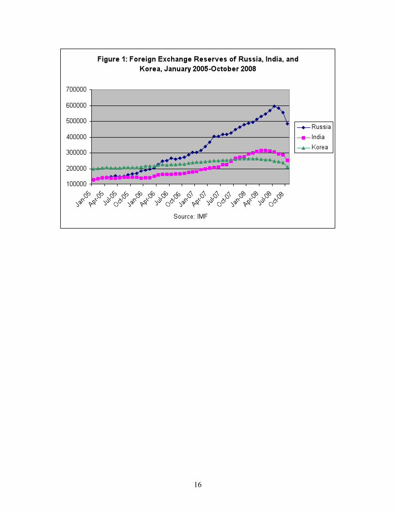
Figure 1 illustrates reserve developments for three large emerging economies, the

Russian Federation, India, and Korea. All three countries’ reserve levels peaked and then

began to decline in the summer of 2008. In particular, Russia’s huge reserve holdings—

second in dollar terms only to those of China and Japan—have plummeted by about a

quarter since reaching their oil-driven peak in July 2008.1 There are many other examples

beyond the three especially dramatic ones in Figure 1; often, however, the percentage

reserve losses are smaller (so far) and start later (for example, after the September 2008

Lehman Brothers collapse). The Russian, Indian, and Korean currencies have all

depreciated against the United States dollar since the summer of 2008, with Korea’s won

declining most dramatically to levels not seen since the Asian crisis of the late 1990s.

Before the recent crisis, commentary on the emerging-market reserve buildup

focused on the possibility that reserve stocks might have reached “excessive” levels.

Certainly some countries’ reserve levels far exceeded the levels needed to counter

fluctuations in export earnings, and often even covered the possibility that short-term

1 The Russian situation was exacerbated by noneconomic fundamentals (political risk), most notably following the invasion of Georgia in August 2008. The Russian data are also obfuscated by occasional replenishments of the central bank’s reserves by drawing from the country’s Sovereign Wealth Fund. The fungibility of central bank and SWF assets, and the rapidly growing size of SWF hoards, will likely complicate measurement even further in future.

2

external debts might not be rolled over (the so-called “Guidotti-Greenspan” prescription

for reserve adequacy). Economic analysis of optimal reserve levels has a long history,

going back at least to the writing of Henry Thornton (1939) at the start of the nineteenth

century. In recent work, we have followed Thornton’s lead, arguing that governments—

especially those of emerging markets—view reserves as protection against “double-

drain” crisis scenarios in which banking and currency problems interact in ways likely to

cause sharp and disruptive external currency depreciation.2

In a specific crisis scenario, investor fear of currency depreciation leads to a run

out of domestic deposits, pressuring banks and triggering lender-of-last resort liquidity

(LLR) provision by the monetary authorities. This LLR support, however, magnifies the

potential claims on official foreign exchange reserves, and hence magnifies the currency

depreciation that results when the reserves are expended to support the exchange rate. It

follows that reserve levels may have to be quite large if the banking system is highly

developed and the government hopes to resist sharp currency depreciation in a potential

crisis. Official fear of abrupt depreciation may be due to dollarized financial liabilities,

rapid pass-through to inflation, or other factors discussed in the “fear of floating”

literature.

The utility of foreign exchange reserves is well articulated by the International

Monetary Fund (2008, p. 37) in a recent overview of the current crisis: “[I]n the face of

sharp capital outflows, countries will need to respond quickly to ensure adequate liquidity

and deal with emerging problems in weaker institutions. The exchange rate should be

2 See Maurice Obstfeld, Jay C. Shambaugh, and Alan M. Taylor (2008). Similar theoretical ideas have been discussed in the crisis literature, for example by Guillermo A. Calvo (1996, 2006), Calvo and Enrique G. Mendoza (1996), Roberto Chang and Andrés Velasco (2001), Jeffrey D. Sachs (1998), and Velasco (1987). Jeanne (2007) surveys recent commentary and analysis regarding emerging-market reserves.

3

allowed to absorb some of the pressure, but stockpiles of reserves provide room for

intervention to avoid disorderly market conditions.”

I. Financial Stability and Reserves in the Data

In Obstfeld et al. (2008) we argue that a considerable share of the reserve accumulation in

recent years can be explained as an attempt by central banks to insure against this sort of

financial instability. Importantly, the financial shock we consider is not simply a “sudden

stop”, in which case countries would need to hold reserves only in proportion to their

short term external debt. Rather, internal sources of financial instability also can be

critical. As a result, when a country has open financial markets and desires exchange rate

stability, it needs to hold reserves proportional to the size of its banking system.

Specifically, we show that the reserves/GDP ratio is a function of financial

openness, the exchange rate regime and monetary depth (M2/GDP ratio). Despite the

focus on the “Guidotti-Greenspan” rule and sudden stops in the literature, short term

external debt is not a significant predictor of reserve holdings, though another variable

often considered in more traditional models, the Trade/GDP ratio is.3 Thus, a

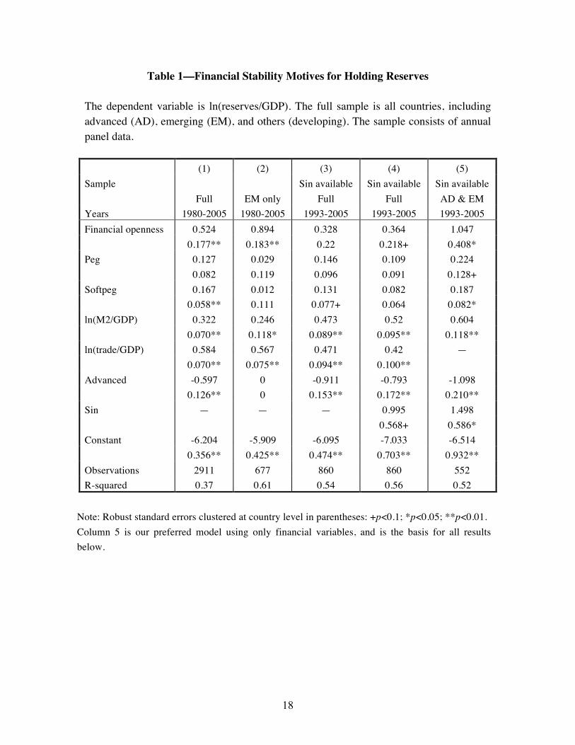
specification like that in Table 1, Column 1, which combines our basic “financial

stability” variables with Trade/GDP does a good job of explaining reserve behavior.4 We

3 For a review of the recent empirical literature, see Obstfeld et al (2008). Robert Flood and Nancy Marion (2002) have connected reserve holdings to a buffer stock model, Joshua Aizenman and Marion (2003) have argued the buildup of reserves in East Asia can be seen as precautionary savings, and Aizenman and Jaewoo Lee (2007) argue that precautionary not mercantilist reasons can explain the reserves buildup. Relative to these papers, we focus more on the size of the domestic financial system as opposed to fear of sudden stops. 4 The model is estimated in natural logs and standard errors are clustered at the country level to correct for both heteroskedasticity across countries and serial correlation within countries. We use WDI data for reserves, GDP, and M2. The Financial openness measure is from Edwards (2007), the exchange rate classification is based on Shambaugh (2004), and the measure of “original sin” is from Barry Eichengreen et al. (2005) and is based on BIS issuance data. See Obstfeld et al. (2008) for details on data and sample.

4

see that the coefficients on financial openness, monetary depth, and trade all have

expected signs and are significantly different from zero at 99%. A “soft peg” measure is

also positive and significant at 99% while a direct peg is not (though the two are not

statistically significantly different). The regressions are in logs, so a 10% increase in the

M2/GDP ratio is correlated with a 3% increase in the reserves to GDP ratio. Financial

openness is scaled between 0 and 1 (based on the measure proposed by Sebastian

Edwards 2007) and the exchange-rate regime variables are dummies.

In the Emerging Market sample (EM), where much of the puzzle over recent

behavior lies, a specification like this explains a substantial portion of reserve/GDP

variation, both over time for one country (in panel estimations with country fixed effects)

and across countries (in cross-sections or in panels with year fixed effects). Column 2

shows the basic EM sample regression. The coefficients on financial openness and

monetary depth are even larger, as is the explanatory power of the regression. The R2 is

now as high as 0.6. Differences in exchange rate regimes are not significant in the EM-

only sample.5

Financial depth is even more important in the last 15 years since the expansion of

financial globalization. In Column 3 we show the specification for 1993-2005 for all

countries.6 Here the coefficient on financial depth has increased such that a 10% increase

in M2/GDP comes with a 5% increase in reserves/GDP. The coefficient on trade

5 As we note in our previous work, many of the emerging market countries flip back and forth across exchange rate regimes and even when not pegging may intend to peg soon. See Michael W. Klein and Shambaugh (2008). 6 As noted below, we will also include a measure of the ability to issue debt externally in local currency. This measure is not available until 1993, so we limit ourselves to that sample here. In Obstfeld et al. (2008) we show that a post 1990 sample that is not limited by “sin” data availability also looks like the regression shown here.

5

openness has declined some. Financial openness is less significant in this sample. There

is less variation within country in this shorter sample so some precision is lost.

One other factor that is consistently significant is a dummy for the advanced

countries (AD). These countries hold fewer reserves than their M2/GDP, Trade/GDP,

exchange rate regime and financial openness suggest they should. This is true even when

we control for the ability to issue debt in ones’ own currency, or “original sin.” Column 4

shows this regression. The sin variable—which varies from 0 (little foreign currency debt

issued) to 1 (all external debt is in foreign currency, none local) has a significant and

positive coefficient. Going from all local currency debt to all foreign currency debt would

double reserve holdings.7

In this paper, rather than focusing entirely on the EM sample (as in our previous

work) we now include AD countries. While the puzzle of reserve buildup was primarily

an EM issue, the current crisis is one that clearly touches both EM and AD countries.

Thus, in our predictive work below will be limited to that sample, for which column 5

shows the corresponding results for our preferred benchmark regression with only

financial variables.

II. Implications for Today

What can our positive empirical model tell us about reserves, central bank swaps of

foreign currency, and exchange rates during the recent financial panic? We want to know

how actual reserve holdings on the eve of the crisis compare to what our model would

predict, to see if countries were “underinsured” or “overinsured.” Thus, we first generate 7 This variable is largely cross-sectional. There is little variation within countries. Further, there is little variation across the EM and developing countries. Nearly all issue almost exclusively foreign currency debt externally. There is, however, cross-country variation within the advanced sample.

6

predicted values for reserve-to-GDP ratios in 2005. We then adjust those ratios for

M2/GDP changes in the last two years to get approximate predicted values for 2007,

since M2 growth is the main regressor that changes at high frequency in our sample.

(More details are shown in Appendix Table 1.)

For the year 2007, EM countries were predicted to hold substantial reserves;

predicted ratios are quite high (20% of GDP on average) relative to those of AD countries

(9%). Some have accumulated far beyond these levels, especially between 2005 and

2007. By 2007, actual reserves were 26% of GDP on average for these countries.8 For

example, in 2005, China’s predicted reserves were 29% of GDP while actual were 37%.

China held more reserves than expected, but not dramatically so. By 2007, however,

predicted reserves had not moved much but China’s actual reserves were up to 47% of

GDP. Likewise Malaysia, Singapore, and Korea were all predicted to have reserves of

20% of GDP or more, but actual levels were substantially higher. Also, countries like

Brazil or India who were at or below predicted levels in 2005 were above them by 2007.

The model predicts the variation across these countries reasonably well. The correlation

of predicted and actual reserve/GDP ratios is 0.68.

On the other hand, we can see that many advanced countries held fewer reserves

than our model predicts.9 Australia, the U.K., and Canada are notable examples. What if

we do not think advanced countries should hold fewer reserves than other countries? That

is, what if we run the regression in column 5 without the AD dummy, we see that the

predicted values (based on the large financial sectors and tendency towards financial

8 Hong Kong and Singapore are both predicted to and do hold far more reserves than other countries. Excluding them, the predicted reserve ratio for the group is 17% of GDP and the actual is 21%. 9 Due to a lack of individual country reserve holdings or M2, euro area countries are not included in the analysis of predicted reserves.

7

openness) suggest the advanced countries should be holding larger stocks of reserves than

they actually own. In this exercise we also find that Denmark, Sweden, and New Zealand

are holding fewer reserves than the typical country with their characteristics. Only Japan

holds substantially more reserves than the predicted value suggests they would.10

Perhaps some advanced countries held too few reserves? On the other hand, many

of these advanced countries received substantial U.S. dollar swap lines from the Federal

Reserve in 2007 and 2008. Perhaps they knew such types of arrangements would be

available to them in a pinch, so they did not feel the need to hold reserves in the same

pattern as EM countries. In that case, estimation with the AD dummy may be the right

benchmark to examine.11

III. Currency Pressure versus the War Chests in The Panic of 2008

Echoing Thornton, our theoretical model assumes that it is in the event of a panic that

reserves will be used to quell M2 flight and avert depreciation. It is natural to ask whether

this mechanism was at work in 2008: were exchange rates better stabilized in countries

with more reserves relative to M2?—or, to be more faithful to the multivariate model,

with more reserves relative to what the model would have predicted?

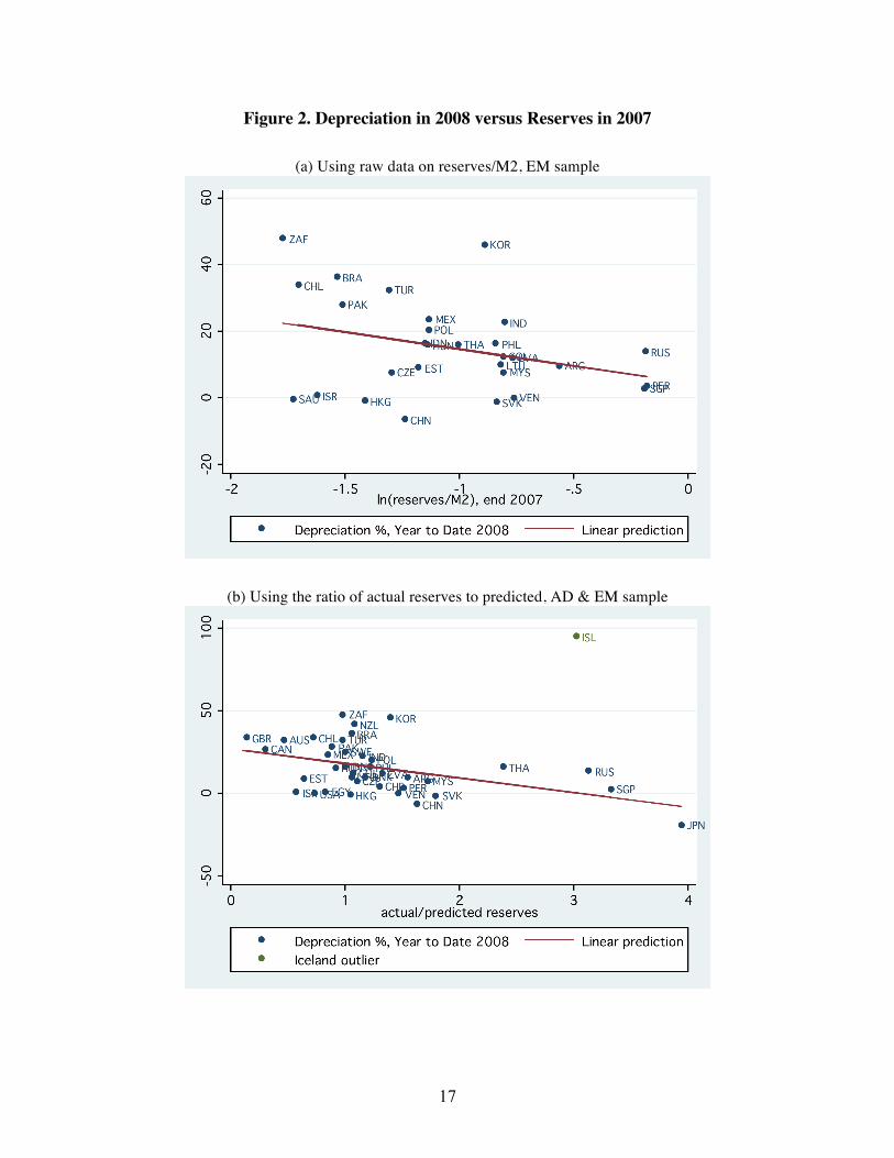
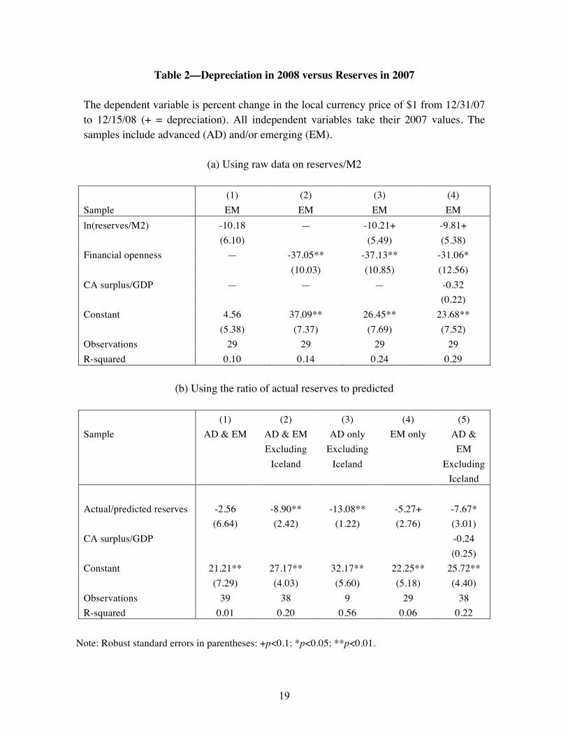
Figure 2a addresses the first of these questions with a simple scatter of percentage

depreciation of the currency against the U.S. dollar in the year 2008 [up to 12/15 at time

10 Iceland’s predicted reserves are lower than some other countries because their financial account is coded as less open than other advanced countries in the Edwards measure. The Chinn-Ito index also codes Iceland as more closed than other advanced nations. 11 Admittedly, some EM countries (surprisingly) received swap lines from the Fed in 2008. However, the size of these lines appears small compared to their hypothetical needs in the event that a run from M2 should materialize. Skeptics have therefore argued that these lines may be signals at best, or pure window dressing. At the time of writing, it is an open question whether they would be expanded, or augmented by IMF lines or other funding, should disaster strike.

8

of writing] versus the country’s reserves/M2 ratio at the end of 2007. The sample is

restricted to just the emerging countries, as our regressions suggest that advanced

countries have an intrinsically smaller need for reserves due to, say, more policy

credibility and certainty, or better access to private credit or official swap lines. The

scatter shows that countries with feebler war chests at the end of 2007 suffered larger

currency crashes in 2008, offering preliminary support for our arguments. However,

Table 2, panel (a) explores this relationship further and adds some controls. Column 1

shows that the bivariate relationship is only borderline significant (p value 0.106). In

contrast to arguments regarding the perils of financial openness, Column 2 shows that

currency values of more financially open economies saw their currency values more

likely to hold in 2008, hinting at reverse causality from (more) financial stability to

(more) openness. Column 3 enters openness and reserves together and the results are

similar. Finally, Column 4 entertains another prevalent explanation, namely that

depreciations are really a result of unsustainable current account deficits. But lagged

current account deficit as a share of GDP was not a highly statistically significant

influence in this sample, once we control for the size of the reserve war chest.12

Table 2, panel (b) takes the next step of using not actual 2007 reserves as a

control variable, but the ratio of actual reserves to what our preferred model would have

predicted. We now see whether “underinsurance” (as judged by our positive model) was

associated with larger depreciations in 2008. Indeed it was in all samples once we

exclude an influential extreme outlier—the infamous case of Iceland. In Columns 2

12 We also experimented in both panels of Table 2 with lagged short term debt to GDP ratio as an extra regressor, to address the claim that rollover problems might exacerbate depreciation, but we found its coefficient always had the wrong (negative) sign, so that bigger debts appeared to be related to smaller depreciations, contradicting the theory.

9

through 5, which unlike Column 1 exclude Iceland, the relationship between low reserves

and high depreciation is clear. Actual relative to predicted reserves is significant at the

1% level in the full and AD samples, and the 10% level in the more noisy EM sample. In

Column 6 this result is again robust to the inclusion of the lagged current account surplus

to GDP ratio, which is once more statistically insignificant (though of the expected sign).

As a convenient graphical summary of our argument, we present a scatter plot of actual

depreciation in 2008 versus our model’s actual/predicted reserve ratio for the AD & EM

sample. This is shown in Figure 2b, with Iceland excluded from the line of best fit, as in

Column 2. Excluding the bizarre case of Iceland, the results are quite striking:

international reserves did provide effective insurance against currency instability, for

both advanced and emerging countries alike.

IV. Central Bank Currency Swaps in the Panic of 2008

This crisis has also generated one of the most notable examples of central bank

cooperation in history—the large swap lines set up between a number of central banks.13

The Federal Reserve extended large swap lines to industrial-country central banks first

(ECB, BoJ, BoE, and SNB) starting in 2007; then extended those to nearly every

advanced economy; and finally, on October 29, 2008, granted similar arrangements to

four major emerging market countries (Brazil, Korea, Mexico, and Singapore).14

In these swaps, the Fed has provided dollar liquidity to the other central banks

allowing these central banks, in turn, to provide dollars to their own domestic banking

systems. Why are such swap lines needed? Two alternatives for the provision of dollar 13 See Setser (2008) for real-time commentary on the extraordinary nature of the measures. 14 See http://www.federalreserve.gov/newsevents/press/monetary/20081029b.htm and links therein for press releases on the swap lines.

10

liquidity in the foreign country would be (a) for the foreign central bank to provide the

domestic currency and let the bank sell the local currency for dollars on the open market

or (b) for the foreign central bank to use its own dollar reserves to provide the liquidity.

The former would put downward pressure on the local currency and the latter would

possibly exhaust the central bank’s dollar reserves. Examining current reserve holdings

relative to our positive model’s predictions is a useful way to provide some empirical

context for these swap lines.

The size of the swap lines available has varied across countries and for the major

industrial-country central banks eventually became unlimited. The ECB and SNB also

instituted smaller swap lines, in their own currencies, with a number of smaller European

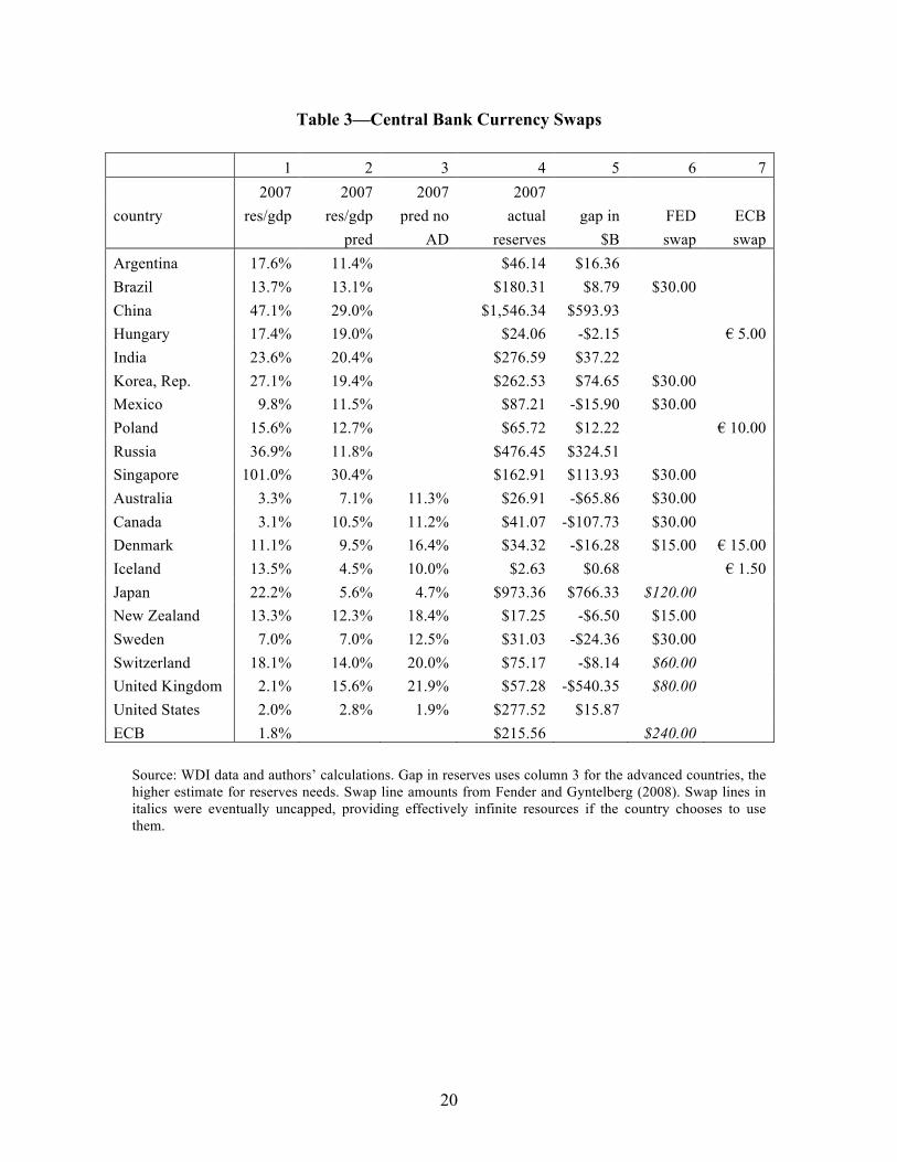
countries.15 In Table 3, for swap recipients, we show actual and predicted reserves/GDP

as well as actual reserves in dollars, the gap in our model between actual to predicted (in

dollars), and the size of the initial swap lines themselves.

The swaps were clearly large in magnitude for many advanced countries. For

every advanced country except Japan, the size of the swap exceeded 50% of actual

reserves held and in the case of the U.K., Australia, and the ECB, the swap was larger

than the existing level of reserves.16 In addition, for a number of countries, such as

Denmark, Sweden, and New Zealand, not only was the swap line nearly as big as existing

reserves, but it was larger than the gap with our model’s prediction. On the other hand, in

some cases, the swap line was too small to plug the gap relative to predicted reserves.

15 See Fender and Gyntelberg (2008) for a discussion of the swap lines. Data for the size of the swaps is taken from there. Swaps that were eventually increased to infinity are listed in the table at the largest amount prior to that increase and are noted in the table. 16 Detailed information on reserves on the Bank of England website shows currency composition of reserves and this reveals that the BoE holdings of US dollars was much smaller than the total reserves and by the time the swap line was instituted, the BoE was down to less than $10 billion in US dollar reserves.

11

Australia, Canada and the U.K. all still have fewer reserves than expected even counting

the swap (and not counting the decline in their reserves in 2008 so far).

In contrast, the swaps to emerging countries are never larger than 50% of their

actual reserves. Further, in most cases, the country already had more reserves than

predicted. Korea’s was $30 billion, though the country already had $260 billion. For

Singapore the figure was, $30 billion against $162 billion already held, and Brazil

received $30 billion versus $180 billion on hand. It is hard to see how these magnitudes

could be very meaningful; all three countries already held more reserves than predicted

by our model. Instead, these swap lines could be interpreted as signals. For Mexico and

Hungary, the swaps are more substantial relative to actual reserves and those two

countries were holding fewer reserves than predicted, so the swap lines may have had a

more substantive impact beyond mere signaling in those cases.

This way of looking at the swaps demonstrates a number of important issues in

the current international monetary system. Even with nearly a trillion dollars committed,

in some cases the Fed’s action was primarily symbolic because the foreign country

already had so many dollars. In other cases, the swap may have been quite important, but

the scale required to for effective lending is not available to organizations such as the

IMF or other multilateral agencies. Only the world’s largest central banks can intervene

on such a scale. Some players (such as China and India) do have foreign reserves

sufficient to allow them to act as crisis lenders to foreign governments, but so far such

actions have been limited, including Nordic central banks lending euros to Iceland and

Japan’s offer of $100 billion in resources to the IMF.

12

The swap lines also have implications for reserve holdings. One could argue that

the expectation that such swap lines could be available rationalizes advanced countries’

decisions to hold fewer reserves than other countries. This would suggest EM countries

will continue to hold large reserves until they are confident that they will have access to

substantial foreign exchange swaps when in need. Alternatively, these extraordinary

measures may have been just that—extraordinary. The advanced countries may now

recognize this and increase their reserve stocks (or in some cases adopt the euro to

reduce the need for reserves). An increase in IMF resources could also be in the cards.

V. Conclusion

International reserves are in some ways the ultimate rainy day fund for a country. They

are hard, liquid assets that have value in times of need. The Panic of 2008 is more than a

rainy day: it is a torrential downpour. Elsewhere we have argued that reserve holdings are

strongly connected to the size of the banking system. Countries insure not just against an

end of foreign financial inflows, but also against runs on the currency by domestic savers.

Here we show that interpreting reserve holdings in this manner is helpful for

understanding reserve adequacy and countries’ seemingly different abilities to weather

the current storm.

Currencies of countries holding more reserves relative to M2—and in particular,

more reserves relative to our measure of predicted reserves based on financial motives—

have tended to appreciate in the crisis. Those of countries with smaller war chests have

depreciated. Understanding these motives for reserve demand also shows that central

bank swap lines to some smaller advanced countries have been sizable as a share of

13

current and needed reserves. For most EM countries, though, the swaps have been largely

symbolic. The scale of reserves needed to backstop emerging markets simply surpasses

the resources of the multilateral organizations and all but the largest reserves holders in

the world.

REFERENCES

Aizenman, Joshua, and Jaewoo Lee. 2007. “International Reserves: Precautionary

versus Mercantilist Views, Theory and Evidence.” Open Economies Review,

18(2): 191–214.

Aizenman, Joshua, and Nancy Marion. 2003. “The High Demand for International

Reserves in the Far East: What’s Going On?” Journal of the Japanese and

International Economies, 17 (September): 370–400.

Calvo, Guillermo A. 1996. “Capital Flows and Macroeconomic Management: Tequila

Lessons.” International Journal of Finance and Economics, 1 (July): 207–23.

Calvo, Guillermo A. 2006. “Monetary Policy Challenges in Emerging Markets: Sudden

Stop, Liability Dollarization, and Lender of Last Resort.” Working Paper 12788,

National Bureau of Economic Research.

Calvo, Guillermo A., and Enrique G. Mendoza. 1996. “Mexico’s Balance-of-

Payments Crisis: A Chronicle of a Death Foretold.” Journal of International

Economics, 41 (November): 235–64.

Chang, Roberto, and Andres Velasco. 2001. “Financial Crises in Emerging Markets: A

Canonical Model.” Quarterly Journal of Economics, 116: 489–517.

14

Edwards, Sebastian. 2007. “Capital Controls, Sudden Stops, and Current Account

Reversals.” In Capital Controls and Capital Flows in Emerging Economies:

Policies, Practices, and Consequences, ed. S. Edwards. Chicago: University of

Chicago Press.

Eichengreen, Barry, Ricardo Hausmann, and Ugo Panizza. 2005. “The Pain of

Original Sin.” In Other Peoples’ Money, ed. B. Eichengreen and R. Hausmann,

13–47. Chicago: University of Chicago Press.

Fender, Ingo, and Jacob Gyntelberg. 2008. “Overview: Global Financial Crisis Spurs

Unprecedented Policy Actions.” BIS Quarterly Review, December.

Flood, Robert, and Nancy Marion. 2002. “Holding International Reserves in an Era of

High Capital Mobility.” In Brookings Trade Forum 2001, ed. S. M. Collins and

D. Rodrik, 1–68. Washington, DC: Brookings Institution.

International Monetary Fund. 2008. World Economic Outlook: Financial Stress,

Downturns, and Recoveries. Washington, DC: International Monetary Fund.

Jeanne, Olivier. 2007. “International Reserves in Emerging Market Countries: Too

Much of a Good Thing?” Brookings Papers on Economic Activity, 1: 1–79.

Klein, Michael W., and Jay C. Shambaugh. 2008. “The Dynamics of Exchange Rate

Regimes: Fixes, Floats, and Flips.” Journal of International Economics 75(1):

70–92.

Obstfeld, Maurice, Jay C. Shambaugh, and Alan M. Taylor. 2008. “Financial

Stability, the Trilemma, and International Reserves.” NBER Working Paper no.

14217.

15

Sachs, Jeffrey D. 1998. “Creditor Panics: Causes and Remedies.” Photocopy. Harvard

University (October). http://www.cid.harvard.edu/archive/hiid/papers/cato.pdf.

Setser, Brad. 2008. “More extraordinary moves: $620 billion is real money, and it isn’t

even for American financial institutions …”, http://blogs.cfr.org/

setser/2008/09/29/more-extraordinary-moves-620-billion-is-real-money-and-it-

isnt-even-for-american-financial-institutions/.

Shambaugh, Jay C. 2004. “The Effects of Fixed Exchange Rates on Monetary Policy.”

Quarterly Journal of Economics, 119(1): 301–52.

Thornton, Henry. 1939 [1802]. An Enquiry into the Nature and Effects of the Paper

Credit of Great Britain. Edited with an introduction by F. A. von Hayek. London:

George Allen and Unwin.

Velasco, Andres. 1987. “Financial Crises and Balance of Payments Crises: A Simple

Model of Southern Cone Experience.” Journal of Development Economics, 27:

263–83.

16

17

Figure 2. Depreciation in 2008 versus Reserves in 2007

(a) Using raw data on reserves/M2, EM sample

(b) Using the ratio of actual reserves to predicted, AD & EM sample

18

Table 1—Financial Stability Motives for Holding Reserves The dependent variable is ln(reserves/GDP). The full sample is all countries, including advanced (AD), emerging (EM), and others (developing). The sample consists of annual panel data.

(1) (2) (3) (4) (5) Sample

Full

EM only Sin available

Full Sin available

Full Sin available AD & EM

Years 1980-2005 1980-2005 1993-2005 1993-2005 1993-2005 Financial openness 0.524 0.894 0.328 0.364 1.047

0.177** 0.183** 0.22 0.218+ 0.408* Peg 0.127 0.029 0.146 0.109 0.224

0.082 0.119 0.096 0.091 0.128+ Softpeg 0.167 0.012 0.131 0.082 0.187

0.058** 0.111 0.077+ 0.064 0.082* ln(M2/GDP) 0.322 0.246 0.473 0.52 0.604

0.070** 0.118* 0.089** 0.095** 0.118** ln(trade/GDP) 0.584 0.567 0.471 0.42 —

0.070** 0.075** 0.094** 0.100** Advanced -0.597 0 -0.911 -0.793 -1.098

0.126** 0 0.153** 0.172** 0.210** Sin — — — 0.995 1.498

0.568+ 0.586* Constant -6.204 -5.909 -6.095 -7.033 -6.514

0.356** 0.425** 0.474** 0.703** 0.932** Observations 2911 677 860 860 552 R-squared 0.37 0.61 0.54 0.56 0.52

Note: Robust standard errors clustered at country level in parentheses: +p<0.1; *p<0.05; **p<0.01. Column 5 is our preferred model using only financial variables, and is the basis for all results below.

19

Table 2—Depreciation in 2008 versus Reserves in 2007 The dependent variable is percent change in the local currency price of $1 from 12/31/07 to 12/15/08 (+ = depreciation). All independent variables take their 2007 values. The samples include advanced (AD) and/or emerging (EM).

(a) Using raw data on reserves/M2 (1) (2) (3) (4) Sample EM EM EM EM ln(reserves/M2) -10.18 — -10.21+ -9.81+ (6.10) (5.49) (5.38) Financial openness — -37.05** -37.13** -31.06* (10.03) (10.85) (12.56) CA surplus/GDP — — — -0.32 (0.22) Constant 4.56 37.09** 26.45** 23.68** (5.38) (7.37) (7.69) (7.52) Observations 29 29 29 29 R-squared 0.10 0.14 0.24 0.29

(b) Using the ratio of actual reserves to predicted (1) (2) (3) (4) (5) Sample AD & EM AD & EM

Excluding Iceland

AD only Excluding

Iceland

EM only

AD & EM

Excluding Iceland

Actual/predicted reserves -2.56 -8.90** -13.08** -5.27+ -7.67* (6.64) (2.42) (1.22) (2.76) (3.01) CA surplus/GDP -0.24 (0.25) Constant 21.21** 27.17** 32.17** 22.25** 25.72** (7.29) (4.03) (5.60) (5.18) (4.40) Observations 39 38 9 29 38 R-squared 0.01 0.20 0.56 0.06 0.22

Note: Robust standard errors in parentheses: +p<0.1; *p<0.05; **p<0.01.

20

Table 3—Central Bank Currency Swaps

1 2 3 4 5 6 7

2007 2007 2007 2007

country res/gdp res/gdp

pred

pred no

AD

actual

reserves

gap in

$B

FED

swap

ECB

swap

Argentina 17.6% 11.4% $46.14 $16.36

Brazil 13.7% 13.1% $180.31 $8.79 $30.00

China 47.1% 29.0% $1,546.34 $593.93

Hungary 17.4% 19.0% $24.06 -$2.15 € 5.00

India 23.6% 20.4% $276.59 $37.22

Korea, Rep. 27.1% 19.4% $262.53 $74.65 $30.00

Mexico 9.8% 11.5% $87.21 -$15.90 $30.00

Poland 15.6% 12.7% $65.72 $12.22 € 10.00

Russia 36.9% 11.8% $476.45 $324.51

Singapore 101.0% 30.4% $162.91 $113.93 $30.00

Australia 3.3% 7.1% 11.3% $26.91 -$65.86 $30.00

Canada 3.1% 10.5% 11.2% $41.07 -$107.73 $30.00

Denmark 11.1% 9.5% 16.4% $34.32 -$16.28 $15.00 € 15.00

Iceland 13.5% 4.5% 10.0% $2.63 $0.68 € 1.50

Japan 22.2% 5.6% 4.7% $973.36 $766.33 $120.00

New Zealand 13.3% 12.3% 18.4% $17.25 -$6.50 $15.00

Sweden 7.0% 7.0% 12.5% $31.03 -$24.36 $30.00

Switzerland 18.1% 14.0% 20.0% $75.17 -$8.14 $60.00

United Kingdom 2.1% 15.6% 21.9% $57.28 -$540.35 $80.00

United States 2.0% 2.8% 1.9% $277.52 $15.87

ECB 1.8% $215.56 $240.00

Source: WDI data and authors’ calculations. Gap in reserves uses column 3 for the advanced countries, the higher estimate for reserves needs. Swap line amounts from Fender and Gyntelberg (2008). Swap lines in italics were eventually uncapped, providing effectively infinite resources if the country chooses to use them.

21

Appendix Table 1—Reserve Holdings in 2007: Predicted versus Actual

1 2 3 4 5 6 7 2007 2007 2007 2005 2005 2007 2008

country_name res/gdp res/gdp pred

res/gdp pred

res/gdp res/gdp pred

actual/pred dner

Argentina 17.6% 11.4% 15.4% 11.5% 155% 5.3% Brazil 13.7% 13.1% 6.8% 12.6% 105% 21.6% Chile 10.3% 14.2% 14.7% 13.9% 72% 26.4% China 47.1% 29.0% 37.3% 29.0% 162% -6.5% Colombia 12.2% 11.5% 12.3% 12.4% 106% 16.0% Czech Republic 20.8% 18.9% 23.9% 18.3% 110% 7.0% Egypt, Arab Rep. 25.1% 30.4% 24.5% 30.8% 83% 1.0% Estonia 15.4% 24.0% 14.9% 22.9% 64% 13.4% Hong Kong, China 73.9% 70.7% 69.7% 66.9% 105% -0.7% Hungary 17.4% 19.0% 17.1% 18.1% 92% 18.3% India 23.6% 20.4% 17.1% 21.3% 116% 23.4% Indonesia 13.2% 13.2% 12.1% 13.7% 100% 15.6% Israel 17.6% 30.8% 22.8% 32.6% 57% -0.3% Korea, Rep. 27.1% 19.4% 26.8% 19.9% 140% 41.9% Latvia 21.2% 16.0% 14.9% 15.2% 133% 16.1% Lithuania 20.1% 19.1% 14.9% 17.6% 106% 14.3% Malaysia 56.4% 32.8% 54.2% 33.5% 172% 7.2% Mexico 9.8% 11.5% 9.6% 11.2% 85% 17.6% Pakistan 11.0% 12.4% 10.0% 12.3% 89% 31.9% Peru 25.5% 16.9% 17.9% 16.6% 151% 2.4% Philippines 23.4% 19.2% 18.7% 18.9% 122% 17.7% Poland 15.6% 12.7% 14.1% 11.9% 123% 14.6% Russian Federation 36.9% 11.8% 23.8% 10.3% 314% 10.0% Singapore 101.0% 30.4% 99.1% 29.6% 333% 2.7% Slovak Republic 25.3% 14.1% 33.4% 14.4% 180% 3.6% South Africa 11.9% 12.1% 8.6% 11.3% 98% 44.3% Thailand 35.6% 14.9% 29.4% 15.6% 239% 16.3% Turkey 11.6% 12.0% 14.5% 12.7% 97% 30.3% Venezuela, RB 14.8% 10.1% 21.3% 8.4% 147% 0.3% Australia 3.3% 7.1% 11.3% 5.9% 6.3% 46% 29.2% Canada 3.1% 10.5% 11.2% 3.0% 10.6% 30% 19.6% Denmark 11.1% 9.5% 16.4% 13.1% 8.8% 118% 14.7% Iceland 13.5% 4.5% 10.0% 6.8% 4.5% 303% 113.9% Japan 22.2% 5.6% 4.7% 18.7% 5.7% 395% -12.7% New Zealand 13.3% 12.3% 18.4% 8.2% 11.5% 108% 29.9% Sweden 7.0% 7.0% 12.5% 7.0% 6.6% 100% 22.4% Switzerland 18.1% 14.0% 20.0% 15.7% 13.9% 130% 3.6% United Kingdom 2.1% 15.6% 21.9% 2.0% 14.3% 13% 25.9% United States 2.0% 2.8% 1.9% 1.5% 2.6% 73% 0.0% Source: WDI data and authors’ calculations. Column 6, actual reserves to predicted reserves uses column 2, the predicted reserves based on column 5 of table 1 for both the advanced and emerging countries. Using the higher estimate for reserves needs for AD countries strengthens the results in table 2b.