No Credit, No Gain: Trade Liberalization Dynamics,

Production Inputs, and Financial Development∗

David Kohn

Pontificia Universidad Catolica de Chile

Fernando Leibovici

Federal Reserve Bank of St. Louis

Michal Szkup

University of British Columbia

March 2022

Abstract

We study the role of financial development on the aggregate and welfare impli-

cations of reducing import tariffs on capital and intermediate inputs. We document

that financially underdeveloped economies feature a slower aggregate response follow-

ing trade liberalization. We set up a quantitative general equilibrium model with

heterogeneous firms subject to collateral constraints and estimate it to match salient

features from Colombian plant-level data. Our model explains a substantial fraction

of the differences in the empirical responses of GDP, consumption, and capital across

economies with different levels of financial development. Slow adjustment due to col-

lateral constraints reduces welfare gains from trade liberalization.

Keywords: financial development, trade liberalization, welfare, production inputs.

JEL: F1, F4.

∗This paper supersedes a previous version titled “Financial Development and Trade Liberalization.” Wethank George Alessandria for helpfully discussing an earlier version of this paper and B. Ravikumar, KimRuhl, and Michael Waugh for helpful comments. We thank Marcela Eslava, Franz Hamann, and DanielOsorio for their help and advice on various aspects of the Colombian data. We also thank participantsat numerous seminars, workshops, and conferences. We thank Alvaro Cordero, Gonzalo Garcia, VicenteJimenez, Jason Dunn, and Matthew Famiglietti for excellent research assistance. David Kohn acknowledgesfinancial support from CONICYT, FONDECYT Regular 1211523. The views expressed in this paper arethose of the individual authors and do not necessarily reflect official positions of the Federal Reserve Bank ofSt. Louis, the Federal Reserve System, or the Board of Governors. Emails: davidkohn@uc.cl (correspondingauthor), fleibovici@gmail.com, michal.szkup@ubc.ca. Address: Pontificia Universidad Catolica de Chile,Instituto de Economıa, piso 3, Av. Vicuna Mackenna 4860, Santiago, Chile.

1 Introduction

A key channel through which openness to international trade promotes growth and economic

development is cheaper production inputs. Cheaper access to imports of physical capital and

intermediate inputs allows firms to accumulate capital and increase productivity, leading

to increased real GDP, investment, and consumption (Amiti and Konings 2007; Wacziarg

and Welch 2008; Estevadeordal and Taylor 2013). Despite these potential benefits, trade

liberalization is often resisted as a means to promote economic development, particularly in

less-developed economies. In this paper, we investigate whether these economies have less

to gain from trade liberalization.

Our starting point is novel empirical evidence showing that frictions in financial markets

may limit the gains from lowering international trade barriers. We document that, following

a reduction in import tariffs, financially underdeveloped economies grow substantially slower

than financially developed ones. These findings suggests that credit market frictions, a salient

feature of developing economies, limit the degree to which firms adjust their production in

response to lower prices of imported intermediates and physical capital, thereby reducing

the gains from trade liberalization in these economies.1

Motivated by this evidence, we set up a general equilibrium model of international trade

with heterogeneous firms and financial frictions to quantify the role of financial development

on the dynamics following trade liberalization. Importantly, our model is designed to capture

the significant role of trade in allowing firms to access cheaper capital and production inputs.

We estimate the model to match salient features of plant-level data for Colombia and use it

to investigate the impact of reducing tariffs on capital and intermediate inputs. We find that

low financial development significantly limits the impact of lowering tariffs on production

inputs, reducing the welfare gains from trade liberalization. Moreover, our model accounts

for a substantial fraction of the empirical dynamics following trade liberalization across

countries that differ in financial development.

Our paper contributes to the literature along three dimensions. First, we document that

financially underdeveloped economies grow relatively slower than their financially developed

counterparts after trade liberalization. Our second contribution is to quantify the extent to

which cross-country differences in financial development account for the observed differences

in aggregate dynamics following trade liberalization. Importantly, our findings show that

accounting for the importance of capital and intermediates in international trade plays a

fundamental role on the dynamics following trade liberalization and how these are shaped

1See Manova (2010) for a review of theoretical and empirical developments on the role of credit constraintsin the adjustment to trade reform.

2

by financial frictions. Our third contribution is to investigate the implications of these

findings for both aggregate welfare as well as for the distribution of welfare gains across

various population subgroups.

We begin by documenting that financially underdeveloped economies grow more slowly

than their financially developed counterparts after reducing import tariffs. Our empirical ap-

proach extends the analysis conducted by Estevadeordal and Taylor (2013) and investigates

the role of financial development on the dynamics of key aggregate outcomes following trade

liberalization. We find that financially underdeveloped economies feature persistently slower

responses of GDP, consumption, and capital following trade liberalization. In particular, we

find that 15 years after trade liberalization, GDP, consumption, and capital are 25% to 40%

larger on average across financially developed economies versus approximately 10% larger

on average across financially underdeveloped economies.

We show that these differences in the post-liberalization dynamics across economies with

different levels of financial development are robust to controlling for pre-liberalization differ-

ences in institutional quality and economic development as well as to controlling for other

potential changes that might have taken place in parallel to trade liberalization such as

changes in financial development and institutional quality. As standard across empirical

analyses based on observational data, other variables might nevertheless remain omitted,

potentially biasing some of our findings.

We investigate the role of financial development in accounting for these findings by setting

up a quantitative general equilibrium model of international trade with frictions in financial

markets. Our model consists of a small open economy populated by entrepreneurs who are

heterogeneous in productivity, can trade internationally, and are subject to financing con-

straints. Entrepreneurs produce differentiated varieties that they can sell both domestically

and abroad, subject to fixed and variable trade costs as in Melitz (2003). Production re-

quires physical capital, labor, and intermediate inputs (i.e., materials), and entrepreneurs

face a collateral constraint that limits the amount they can borrow. Capital and materials

are produced using both domestic and imported varieties, with the latter subject to tariffs.

We estimate the model to match key features of Colombian plant-level data and use

it to quantify the role of credit frictions in shaping the economy’s response to lower tar-

iffs on imports of capital and intermediate inputs. We contrast our findings relative to a

counterfactual economy with developed financial markets parametrized to resemble financial

development in the U.S. Consistent with the data, we find that differences in financial devel-

opment significantly reduce the short- and long-run impacts of trade liberalization on GDP,

consumption, and capital. These findings show that improved access to production inputs

has a fundamentally different impact across economies that differ in financial development.

3

Lower import tariffs on capital and intermediates allow firms to access these goods at

a lower cost, leading them to increase their production scale. Access to finance allows

firms to accumulate physical capital in order to achieve their optimal scale. Therefore, in

economies with underdeveloped financial markets, the adjustment of firms’ production scale

in response to trade liberalization is substantially slower — and thus are the responses of

aggregate output, consumption, and capital. In particular, we find that 10 years after trade

liberalization GDP, capital, and consumption only reach 56%, 50%, and 45%, respectively, of

the transition to the post-liberalization steady state. In contrast, in the financially developed

economy these values are 85%, 83%, and 77%, respectively.

We then contrast the aggregate dynamics implied by the model with their empirical

counterparts as described above. We investigate the responses of key aggregate variables

(GDP, capital, and consumption) to a 20-percentage-point reduction in tariffs on imports of

capital and intermediates inputs, as observed in Colombia over 1988-1992. We find that our

model accounts for a significant fraction of the patterns observed in the data. Over the 15

years following trade liberalization, the model accounts for 16% of the empirical difference in

GDP dynamics between the financially developed and underdeveloped economies. Similarly,

the model accounts for 17% and 46% of the differences in consumption and capital dynamics,

respectively, due to financial development observed in the data over the 15 years following

trade liberalization.

We find that cross-country differences in financial development have significant impli-

cations for the welfare and distributional effects of trade liberalization. First, we show

that the welfare gains from trade liberalization are larger in financially developed economies

(3.0% in consumption-equivalent units vs. 0.5% in the financially underdeveloped econ-

omy) since firms in these economies are able to reap the benefits from trade liberalization

more quickly than those in financially underdeveloped economies. Second, we find that fi-

nancial frictions exacerbate the unequal distribution of the gains from trade liberalization:

These are larger among productive firms that are financially constrained, as cheaper capital

and intermediate inputs relax their borrowing constraints, allowing them to increase their

scale of operation. Moreover, welfare gains are larger across wealthy entrepreneurs (1.7%

in consumption-equivalent units for wealthy entrepreneurs vs. 0.5% for poor ones in the

baseline) and exporters (2.4% for exporters vs. 0.5% for non-exporters in the baseline).

We additionally decompose the welfare effects of trade liberalization to identify the key

channels that account for our results. Our findings show, on the one hand, that the decline

in tariff revenue (which is redistributed lump-sum across agents) has a particularly negative

impact on the welfare of low-income agents and non-exporters, since this revenue represents

a larger proportion of their income. On the other hand, changes in the real exchange rate and

4

the price of capital have a positive impact on welfare, especially for exporters and wealthy

agents. Higher wages help redistribute some of these welfare gains towards poor agents and

non-exporters; this channel is stronger in the financially developed economy. This analysis

contributes to recent studies on the unequal distribution of gains from trade (Autor et al.

2014, 2016; Carroll and Hur 2020a,b; among others).

We then use our model to quantify the effects of the tariff reduction implemented in

Colombia in the early 1990s and investigate the extent to which financial underdevelop-

ment might have slowed down the post-liberalization adjustment. To account for other

potentially omitted factors that might have affected the economy at the time of trade liber-

alization, this alternative quantitative experiment considers the impact of additional shocks

chosen to match the observed dynamics of real GDP, the investment-to-GDP ratio, and the

consumption-to-GDP ratio in Colombia from 1991 to 1995. Our findings suggest that trade

liberalization in Colombia explains more than half of the growth between 1991 and 1995.

In particular, by 1995, the decrease in capital goods tariffs explained 3.1 percentage points

of the 5.7-percentage-points growth in observed GDP. In the financially developed economy,

instead, GDP growth by 1995 due to trade liberalization would have been equal to 7.7 per-

centage points. That is, our model suggests that if Colombia would have had the level of

financial development of the U.S. at the time of trade liberalization, GDP would have been

4.6 percentage points higher than it was in 1995, mostly due to a larger investment boom.

Overall, our findings provide a rationale for the higher resistance to trade liberalization

in less-developed economies: There might simply be less to gain from trade openness in these

economies, particularly in the short and medium run, given the frictions in financial markets

that slow down the adjustment to the post-liberalization environment.

Our paper contributes to several strands of the literature. First, we contribute to a broad

empirical literature on the aggregate impact of trade liberalization. Previous studies, such as

Sachs et al. (1995), Wacziarg and Welch (2008), and Estevadeordal and Taylor (2013), argue

that trade liberalization leads to higher GDP and investment.2 We build on these studies to

show that the previously documented effects of trade liberalization vary systematically with

a country’s pre-liberalization characteristics, such as the level of financial development. In

particular, we show that the previously documented positive effects of trade liberalization

are relatively larger in economies with developed financial markets.3

Second, our paper connects insights from growing literatures on the impact of reducing

trade barriers on imported intermediate inputs (Amiti and Konings 2007) and capital goods

2See also Pavcnik (2002), Goldberg et al. (2009), and Topalova and Khandelwal (2011). Irwin (2019)surveys recent empirical work on the effects of lower import barriers on economic growth.

3Thus, our paper also relates to the literature on the effects of international financial integration; seeSaffie et al. (2020), Tetenyi (2021), and references therein.

5

(Anderson et al. 2015; Ravikumar et al. 2019) with those from studies that investigate the

role of financial development on trade liberalization (Brooks and Dovis 2020; Caggese and

Cunat 2013; Kohn et al. 2016). We contribute to the former by showing that the impact

of reducing trade barriers on imported intermediates and capital goods may significantly

depend on a country’s level of financial development and to the latter by showing that the

role of financial development on the effect of trade liberalization depends critically on the

types of goods included in the trade reform. In particular, our model allows us to separate

the effect of reducing tariffs on capital and intermediate inputs from the effect of reducing

tariffs on consumption goods. Our results suggest that most of the gains from trade are

driven by reducing tariffs on the former.

Finally, our paper contributes to a large literature that studies the aggregate consequences

of financial frictions. Buera et al. (2011), Midrigan and Xu (2014), and Moll (2014) show that

financial frictions induce capital misallocation, leading to potentially significant aggregate

distortions. Chaney (2016), Manova (2013), Kohn et al. (2016, 2020), Brooks and Dovis

(2020), and Leibovici (2021), among others, study the impact of financial frictions on trade

flows.4 This paper extends these frameworks to study the role of credit market frictions on

the impact of reducing tariffs on imports of capital and intermediate inputs.

Most closely related to our work is that of Brooks and Dovis (2020), who show that

the role of financial frictions on trade liberalization depends critically on whether borrowing

constraints are backward or forward looking.5 Motivated by the observed pervasiveness of

collateral requirements to access external funds in poor and emerging economies, we model

borrowing frictions as collateral constraints. Thus, while borrowing constraints are likely

to be determined by both backward- and forward-looking forces, we restrict attention to

the former in this study.6 Our paper complements findings of Brooks and Dovis (2020)

by estimating empirically the role of credit market frictions on the dynamics following trade

liberalization across countries as well as by quantifying the role of reduced tariffs on imported

intermediates and capital goods versus consumption in accounting for the observed cross-

country dynamics.

4See Kohn et al. (2022) for a review of this literature.5Also closely related are Caggese and Cunat (2013) and Kohn et al. (2016), though both study the role

of financial frictions on trade liberalization on all goods in a partial equilibrium environment.6We see our approach as complementary to the analysis of forward-looking constraints conducted by

Asturias et al. (2016) and Brooks and Dovis (2020). More work is needed to determine the nature ofborrowing constraints faced by firms in developing versus developed countries.

6

2 Empirical evidence

In this section, we investigate empirically the extent to which aggregate economic dynamics

following trade liberalization differ by level of financial development. Our data and approach

build on the work of Estevadeordal and Taylor (2013), which we extend to investigate the

effect of trade liberalization across a broader set of aggregate outcomes as well as to study

the role of financial development. Following their work, we focus on trade liberalization

episodes that took place between then 1980s and 1990s — the period that they refer to as

the “Great Liberalization” experiment.

2.1 Data

Our empirical analysis employs three types of data. First, we use data on import tariffs

to identify trade liberalization episodes. Second, we use data on the level of financial de-

velopment to contrast countries undergoing trade liberalization under alternative financial

environments. Finally, we use data on aggregate variables. The data used throughout the

analysis is at annual frequency, and we now describe it in more detail.

Import tariffs We measure the degree of trade openness across countries using data on

average import tariffs across all goods. Following Estevadeordal and Taylor (2013), we use

data from the Economic Freedom in the World 2005 database and measure tariffs at two

points in time around the Great Liberalization experiment: before or early in the trade

liberalization process (year 1985) and late in the trade liberalization process or after it took

place (year 2000). Average tariffs are computed without weights.

Financial development We measure the degree of financial development across countries

using the World Bank’s Global Financial Development database (Cihak et al. 2012). We

restrict attention to the amount of domestic credit provided to the private sector as a share

of GDP (GFDD.DI.14), which is a popular measure used in the literature to study the effects

of financial development (see, for example, King and Levine 1993 or Manova 2013).

Aggregate outcomes We use data from the Penn World Tables 9.1 (Feenstra et al. 2015)

to document the dynamics of the following variables: GDP, consumption, capital, investment,

exports, and imports. All variables are per capita and expressed in constant domestic prices.

7

2.2 Trade liberalization dynamics and financial development

We now investigate the extent to which the aggregate dynamics following trade liberalization

differ across countries with different levels of financial development. To identify the effect of

trade liberalization, we control for several sources of confounding effects.

First, countries can differ in their growth trajectories after trade liberalization for reasons

unrelated to tariff changes. For instance, developed economies typically grow more slowly

than emerging economies. We control for differences in medium-term growth trajectories

across countries by detrending all variables in a country relative to the country’s average

growth of real GDP over 1975-1985.

Second, countries differ in the extent to which they open up to trade. Thus, some

countries might feature sharper dynamics following trade liberalization not because of the

role of financial development but rather because they decreased tariffs by more. We control

for cross-country differences in tariff changes by restricting attention to the elasticity of

aggregate economic outcomes to changes in tariffs.

Third, while we are interested in the role of financial development on the effects of trade

liberalization, previous studies have documented that the latter can also affect the former

(Do and Levchenko 2007). We mitigate the potential for reverse causality by measuring a

country’s level of financial development as the average over 1975-1985, that is, prior to the

beginning of the period that we study.

We estimate the average cross-country dynamics following trade liberalization and their

interaction with financial development with the following specification:

∆ ln yit = γ +2000∑

k=1975

I{t=k}[αk ∆ ln τi + βk ∆ ln τi ×

CreditiGDPi

]+ εit, (1)

where subscripts i and t index countries and years, respectively. The dependent variable

∆ ln yit consists of the log-change of variable y in country i and year t relative to 1985, where

y is one of the following six aggregate variables: GDP, consumption, capital, investment,

exports, and imports. The elasticity of y in year k in response to a tariff change ∆ ln τi is

given by αk +βk× CreditiGDPi

, where CreditiGDPi

denotes country i’s average credit-to-GDP ratio prior

to trade liberalization (over the period 1975-1985). Finally, εit is a zero-mean error and I is

an indicator function.

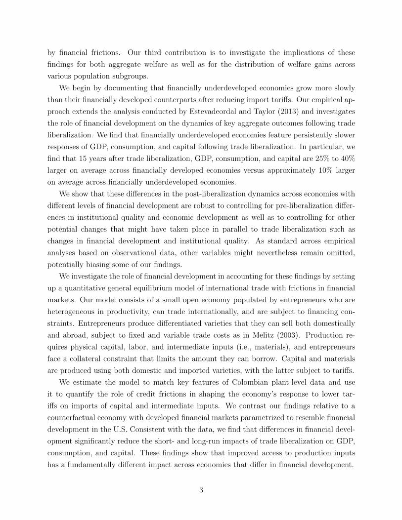
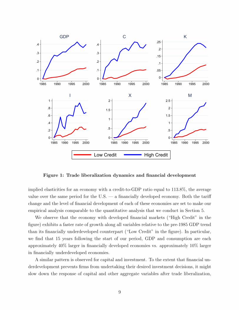
Figure 1 plots the elasticity over time associated with a 20-percentage-point decline in

tariffs for each of the aggregate variables. We present this elasticity for an economy with a

credit-to-GDP ratio equal to 24.9%, the average value observed in Colombia over the period

1986-1990 — an economy with underdeveloped financial markets — and contrast it with the

8

0

.1

.2

.3

.4

1985 1990 1995 2000

GDP

0

.1

.2

.3

.4

1985 1990 1995 2000

C

0

.05

.1

.15

.2

.25

1985 1990 1995 2000

K

0

.2

.4

.6

.8

1

1985 1990 1995 2000

I

0

.5

1

1.5

2

1985 1990 1995 2000

X

0

.5

1

1.5

2

2.5

1985 1990 1995 2000

M

Low Credit High Credit

Figure 1: Trade liberalization dynamics and financial development

implied elasticities for an economy with a credit-to-GDP ratio equal to 113.8%, the average

value over the same period for the U.S. — a financially developed economy. Both the tariff

change and the level of financial development of each of these economies are set to make our

empirical analysis comparable to the quantitative analysis that we conduct in Section 5.

We observe that the economy with developed financial markets (“High Credit” in the

figure) exhibits a faster rate of growth along all variables relative to the pre-1985 GDP trend

than its financially underdeveloped counterpart (“Low Credit” in the figure). In particular,

we find that 15 years following the start of our period, GDP and consumption are each

approximately 40% larger in financially developed economies vs. approximately 10% larger

in financially underdeveloped economies.

A similar pattern is observed for capital and investment. To the extent that financial un-

derdevelopment prevents firms from undertaking their desired investment decisions, it might

slow down the response of capital and other aggregate variables after trade liberalization,

9

decreasing the potential gains from lower tariffs. Consistent with this potential mechanism,

we observe that imports and exports increase substantially more in the financially developed

economy, suggesting that financially underdeveloped economies indeed have a systematically

milder response to similar tariff changes.

These findings suggest that differences in financial development across countries might

have a significant impact on aggregate dynamics following trade liberalization. Next, we

investigate their robustness to controlling for other differences across countries.

2.3 Role of financial development versus other channels

Our above findings suggest that financial development affects aggregate dynamics following

trade liberalization. However, potential omitted variables might be biasing these results.

First, countries may differ in their pre-liberalization initial conditions along dimensions

that (i) are correlated with financial development and (ii) also impact the dynamics following

trade liberalization. For instance, in a country with weak institutions, changes in trade

openness might not have a sizable impact on economic outcomes, as firms and households

might be uncertain about the duration of these changes. Instead, in countries with strong

institutions, governments’ power to arbitrarily change the rules of the game is likely to be

more limited, leading firms and households in these economies to see trade liberalization as

a more persistent reform. Thus, a country’s pre-liberalization institutional quality and level

of economic development may affect its response to trade liberalization.

Second, countries are likely to have undergone several changes beyond trade liberalization

during the period that we study. To the extent that these changes are correlated with (i)

financial development and (ii) the aggregate outcomes that we focus on, these changes can

be additional sources of omitted variables bias. In particular, it is likely that countries

that liberalize trade also introduce other reforms. For instance, countries with low financial

development might be more likely to improve the quality of their financial markets in parallel

to reforms that increase trade openness. These additional financial market reforms are likely

to impact the aggregate outcomes that we study, thus making it harder to identify the effects

of trade liberalization.

Given these potential concerns, we now examine the robustness of the empirical relation

between financial development and the dynamics following trade liberalization, controlling

for some of these factors. To do so, we estimate the following specification:

∆ ln yi = α + β ∆τi + γ HighCreditGDPi + θ [∆τi × HighCreditGDPi] +K∑k=1

ηk ×Xki + εi,

10

where i indexes countries. The dependent variable ∆ ln yi consists of the average log change

of variable y in country i over the period 1990-2000 relative to 1985. Following Estevadeordal

and Taylor (2013), we focus on the period from 1990 onwards to control for the heterogeneous

timing in which trade reforms where introduced during the 1980s. In contrast to the previous

subsection, we simplify the econometric analysis by focusing on the average changes rather

than on the time series dynamics. As above, we estimate the specification for the following

six aggregate outcomes: GDP, consumption, capital, investment, exports, and imports. On

the right-hand side of the specification, α is a constant, ∆τi is the change in average tariffs

between 1985 and 2000, and HighCreditGDPi is an indicator function that is equal to 1 if

country i’s average credit-to-GDP ratio prior to trade liberalization (1975-1985) is above the

median and zero otherwise. Finally, we control for K additional variables{Xki

}Kk=1

.

We control for potential differences in pre-liberalization initial conditions by focusing

on institutional quality and economic development. We measure institutional quality in

1985 as legal and property rights according to the Economic Freedom in the World 2005

database, and we measure economic development using real GDP per capita from the Penn

World Tables 9.1. Specifically, we add the following variables as controls: (i) an institutional

quality indicator that is equal to 1 if above the median and zero otherwise and its interaction

with tariff changes ∆τi, and (ii) a developed country indicator that is equal to 1 if GDP per

capita is above the median and zero otherwise and its interaction with tariff changes ∆τi.

We also control for other potential changes that might have taken place in parallel to trade

liberalization by focusing on changes in financial development and institutional quality.7 To

do so, we add the following variables as controls: (i) the change in the credit-to-GDP ratio

between 1985 and 2000 and its interaction with tariff changes ∆τi over the same period,

and (ii) the log change in the institutional quality index between 1985 and 2000 and its

interaction with tariff changes ∆τi over the same period.

We report our findings in Table 1. Panel A reports the regression estimates without

additional controls. Consistent with the patterns observed in Figure 1, we find that the

relation between tariff changes and the aggregate outcomes that we study is systematically

related to the countries’ level of financial development. These estimates are positive for all

variables, showing that the aggregate outcomes are estimated to increase relatively more

following trade liberalization in economies that are financially developed. These relations

are statistically significant at the 5% level for all variables except for investment and exports

(significant at the 10% level).

Panel B of Table 1 reports our findings controlling for pre-liberalization institutional

7We do not consider changes in economic development given its close link with the outcomes that westudy. Yet, our findings are robust to additionally controlling for changes in economic development.

11

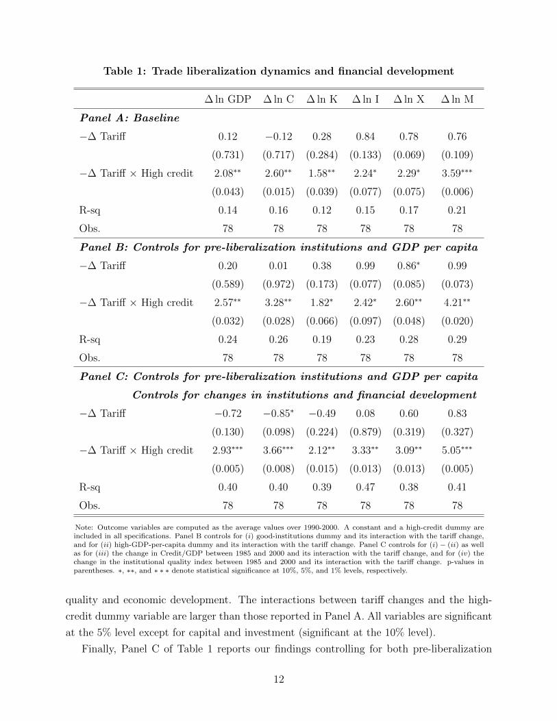
Table 1: Trade liberalization dynamics and financial development

∆ ln GDP ∆ ln C ∆ ln K ∆ ln I ∆ ln X ∆ ln M

Panel A: Baseline

−∆ Tariff 0.12 −0.12 0.28 0.84 0.78 0.76

(0.731) (0.717) (0.284) (0.133) (0.069) (0.109)

−∆ Tariff × High credit 2.08∗∗ 2.60∗∗ 1.58∗∗ 2.24∗ 2.29∗ 3.59∗∗∗

(0.043) (0.015) (0.039) (0.077) (0.075) (0.006)

R-sq 0.14 0.16 0.12 0.15 0.17 0.21

Obs. 78 78 78 78 78 78

Panel B: Controls for pre-liberalization institutions and GDP per capita

−∆ Tariff 0.20 0.01 0.38 0.99 0.86∗ 0.99

(0.589) (0.972) (0.173) (0.077) (0.085) (0.073)

−∆ Tariff × High credit 2.57∗∗ 3.28∗∗ 1.82∗ 2.42∗ 2.60∗∗ 4.21∗∗

(0.032) (0.028) (0.066) (0.097) (0.048) (0.020)

R-sq 0.24 0.26 0.19 0.23 0.28 0.29

Obs. 78 78 78 78 78 78

Panel C: Controls for pre-liberalization institutions and GDP per capita

Controls for changes in institutions and financial development

−∆ Tariff −0.72 −0.85∗ −0.49 0.08 0.60 0.83

(0.130) (0.098) (0.224) (0.879) (0.319) (0.327)

−∆ Tariff × High credit 2.93∗∗∗ 3.66∗∗∗ 2.12∗∗ 3.33∗∗ 3.09∗∗ 5.05∗∗∗

(0.005) (0.008) (0.015) (0.013) (0.013) (0.005)

R-sq 0.40 0.40 0.39 0.47 0.38 0.41

Obs. 78 78 78 78 78 78

Note: Outcome variables are computed as the average values over 1990-2000. A constant and a high-credit dummy areincluded in all specifications. Panel B controls for (i) good-institutions dummy and its interaction with the tariff change,and for (ii) high-GDP-per-capita dummy and its interaction with the tariff change. Panel C controls for (i)− (ii) as wellas for (iii) the change in Credit/GDP between 1985 and 2000 and its interaction with the tariff change, and for (iv) thechange in the institutional quality index between 1985 and 2000 and its interaction with the tariff change. p-values inparentheses. ∗, ∗∗, and ∗ ∗ ∗ denote statistical significance at 10%, 5%, and 1% levels, respectively.

quality and economic development. The interactions between tariff changes and the high-

credit dummy variable are larger than those reported in Panel A. All variables are significant

at the 5% level except for capital and investment (significant at the 10% level).

Finally, Panel C of Table 1 reports our findings controlling for both pre-liberalization

12

institutional quality and economic development as well as for changes in institutional quality

and financial development. The interactions between tariff changes and the high-credit

dummy are now estimated to be even larger than in Panel B. All of these interactions are

positive, as expected, and statistically significant at the 5% level.

These findings suggest that the role of financial development on the dynamics following

trade liberalization documented in Figure 1 is robust to controlling for additional cross-

country differences in pre-liberalization initial conditions as well as for other changes that

might have taken place in parallel to trade liberalization. In fact, the estimated relations

are stronger in both magnitude and statistical significance once we control for these two

additional sources of variation.

Note, however, that this analysis is not exhaustive. It is possible that there are other

sources of cross-country variation that might be simultaneously correlated with financial

development and the aggregate outcomes that we study. In the rest of the paper we address

these concerns by investigating the role of financial development on trade liberalization

quantitatively, using a general equilibrium model of international trade with frictions in

financial markets.

3 Model

We consider a small open economy populated by a unit measure of entrepreneurs, a repre-

sentative producer of composite consumption goods, a representative producer of composite

investment goods, and the rest of the world. Entrepreneurs produce differentiated varieties

by operating a firm and choose whether to sell their output internationally. Composite con-

sumption and investment goods are produced by combining domestic and imported varieties.

Finally, the rest of the world demands the varieties produced by entrepreneurs and is the

source of imported goods.8

3.1 Entrepreneurs

Entrepreneurs are infinitely lived with preferences described by the utility function

E0

∞∑t=0

βtU(ct, ht), (2)

where ct is composite consumption goods, ht is hours worked, β ∈ (0, 1) is the entrepreneurs’

discount factor, and U is a period utility function increasing in consumption, decreasing

8See Section 2 of the Online Appendix for details on the solution of the model.

13

in hours, and concave. E0 denotes the expectation operator taken over the realizations of

productivity shocks, described below, conditional on the information set in period zero.

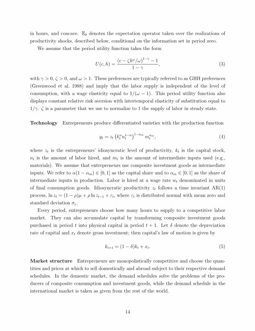
We assume that the period utility function takes the form

U(c, h) =(c− ζhω/ω)1−γ − 1

1− γ, (3)

with γ > 0, ζ > 0, and ω > 1. These preferences are typically referred to as GHH preferences

(Greenwood et al. 1988) and imply that the labor supply is independent of the level of

consumption, with a wage elasticity equal to 1/(ω − 1). This period utility function also

displays constant relative risk aversion with intertemporal elasticity of substitution equal to

1/γ. ζ is a parameter that we use to normalize to 1 the supply of labor in steady state.

Technology Entrepreneurs produce differentiated varieties with the production function

yt = zt(kαt n

1−αt

)1−αmmαmt , (4)

where zt is the entrepreneurs’ idiosyncratic level of productivity, kt is the capital stock,

nt is the amount of labor hired, and mt is the amount of intermediate inputs used (e.g.,

materials). We assume that entrepreneurs use composite investment goods as intermediate

inputs. We refer to α(1− αm) ∈ [0, 1] as the capital share and to αm ∈ [0, 1] as the share of

intermediate inputs in production. Labor is hired at a wage rate wt denominated in units

of final consumption goods. Idiosyncratic productivity zt follows a time invariant AR(1)

process, ln zt = (1− ρ)µ+ ρ ln zt−1 + εt, where εt is distributed normal with mean zero and

standard deviation σε.

Every period, entrepreneurs choose how many hours to supply to a competitive labor

market. They can also accumulate capital by transforming composite investment goods

purchased in period t into physical capital in period t + 1. Let δ denote the depreciation

rate of capital and xt denote gross investment; then capital’s law of motion is given by

kt+1 = (1− δ)kt + xt. (5)

Market structure Entrepreneurs are monopolistically competitive and choose the quan-

tities and prices at which to sell domestically and abroad subject to their respective demand

schedules. In the domestic market, the demand schedules solve the problems of the pro-

ducers of composite consumption and investment goods, while the demand schedule in the

international market is taken as given from the rest of the world.

14

International trade Entrepreneurs can choose to export, but exporting entails additional

variable and fixed costs. Firms pay a fixed cost F , in units of labor, every period that they

export. Furthermore, exporters are subject to an iceberg trade cost τ ≥ 1, which requires

firms to ship τ units for every unit that arrives at a destination. τ captures variable costs

such as shipping costs, foreign marketing costs, or costs due to damages during transit of

goods.

Financial markets Agents have access to international financial markets where they can

borrow or save by trading a one-period risk-free bond at real interest rate r. The interest

rate is taken as given from the rest of the world. However, entrepreneurs face a borrowing

constraint that limits the amount they can borrow: They can only borrow up to a fraction

of the value of the capital stock at the time that the loan is due for repayment.

Let dt+1 denote the amount borrowed by entrepreneur i in period t, due for repayment

in period t+ 1. In addition to the natural borrowing limit, dt+1 has to satisfy

dt+1 ≤ θPk,tkt+1, (6)

where θ ∈ [0, 1] and Pk,t is the price of capital in period t so that Pk,tkt+1 captures the current

price of the total capital stock owned by the entrepreneur.

We denote the net worth of entrepreneurs in period t as at, which is given by at+1 =

Pk,tkt+1 − dt+1/(1 + r).9 Given this definition, the borrowing constraint can be written as

Pk,tkt+1 ≤1 + r

1 + r − θat+1. (7)

Equation (7) shows that the borrowing constraint faced by entrepreneurs limits the amount

of capital that they can operate with. In particular, the current value of next period’s capital

stock has to be lower than a multiple of the entrepreneur’s net worth in period t+ 1.10 Note

also that the tightness of the borrowing constraint is increasing in the price of capital.

Timing The timing of the entrepreneurs’ decisions is as follows. At the beginning of the

period, entrepreneurs hire labor and purchase intermediate inputs to produce their differen-

tiated variety to be sold domestically and possibly also abroad. If they decide to export, they

also pay fixed export costs. Entrepreneurs choose how many hours to work; receive their

9We refer to at interchangeably as net worth or assets.10As discussed below, the entrepreneurs’ net worth in period t + 1 is equal to their savings in period t.

Since kt+1 = (1 − δ)kt + xt, it follows that constraint (7) is actually a constraint on the entrepreneurs’investment in period t. This explains why the capital is priced at price Pk,t rather than Pk,t+1.

15

income from labor, profits, interest, and lump-sum transfers; and then use these resources to

repay debt due from the previous period as well as to consume and save up for next period.

At the end of the period, agents observe the following period’s productivity shock. Then,

they issue debt and choose next period’s level of physical capital given the amount of net

worth they chose to carry over.11

Entrepreneurs’ problem Given the setup described above, the entrepreneurs’ problem

consists of choosing sequences of consumption (ct), supply and demand of labor (ht, nt), inter-

mediates (mt), investment (xt), export status (et), and prices and quantities (yh,t, ph,t, yf,t, pf,t)

at which to sell the varieties in each of the markets (with subscript h denoting the domestic

market and subscript f denoting the foreign market), in order to maximize their lifetime

expected utility. In addition to the borrowing constraint described above and the market-

specific demand schedules described below, entrepreneurs’ choices are subject to a sequence

of period-by-period budget constraints given by

ct + Pk,txt + dt = htwt + [ph,tyh,t + et (ξtpf,tyf,t − wtF )− wtnt − Pk,tmt] +dt+1

1 + r+ Tt, (8)

where ξ is the real exchange rate and Tt is a lump-sum transfer that rebates the import

tariffs revenue.12 Entrepreneurs’ choices are also subject to a sequence of period-by-period

laws of motion for capital, kt+1 = [(1− δ)kt + xt], and production technologies yh,t + τyf,t =

zt(kαt n

1−αt

)1−αmmαmt .

3.2 Composite consumption goods producer

There is a representative producer of composite consumption goods that operates a con-

stant elasticity of substitution technology to aggregate domestic varieties produced by en-

trepreneurs with imported varieties produced by the rest of the world. Each period, the

problem of the producer of composite consumption goods is then given by

maxyh,c,t(i),ym,c,t

Yc,t −∫ 1

0

ph,t(i)yh,c,t(i)di− (1 + τc)ξpm,c,tym,c,t

s.t. Yc,t =

[∫ 1

0

yh,c,t(i)σ−1σ di+ ωcy

σ−1σ

m,c,t

] σσ−1

,

(9)

11Following Buera and Moll (2015), this timing assumption allows us to eliminate uninsured idiosyncraticinvestment risk, thus simplifying the quantitative solution of the model by combining capital, k, and debt,d, into a single state variable: net worth, a, where at+1 = Pk,tkt+1 − dt+1/(1 + r).

12Lump-sum transfers are a common way to rebate tariffs in models with representative agents, but theireffects on the distribution of welfare gains are not innocuous in a model with heterogeneous agents (see, forexample, Carroll and Hur 2020a). In Section 5.2, we discuss their implications for our welfare results.

16

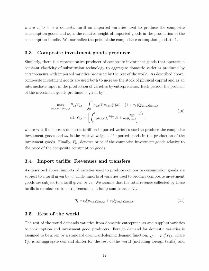
where τc > 0 is a domestic tariff on imported varieties used to produce the composite

consumption goods and ωc is the relative weight of imported goods in the production of the

consumption bundle. We normalize the price of the composite consumption goods to 1.

3.3 Composite investment goods producer

Similarly, there is a representative producer of composite investment goods that operates a

constant elasticity of substitution technology to aggregate domestic varieties produced by

entrepreneurs with imported varieties produced by the rest of the world. As described above,

composite investment goods are used both to increase the stock of physical capital and as an

intermediate input in the production of varieties by entrepreneurs. Each period, the problem

of the investment goods producer is given by

maxyh,k,t(i),ym,k,t

Pk,tYk,t −∫ 1

0

ph,t(i)yh,k,t(i)di− (1 + τk)ξpm,k,tym,k,t

s.t. Yk,t =

[∫ 1

0

yh,k,t(i)σ−1σ di+ ωky

σ−1σ

m,k,t

] σσ−1

,

(10)

where τk > 0 denotes a domestic tariff on imported varieties used to produce the composite

investment goods and ωk is the relative weight of imported goods in the production of the

investment goods. Finally, Pk,t denotes price of the composite investment goods relative to

the price of the composite consumption goods.

3.4 Import tariffs: Revenues and transfers

As described above, imports of varieties used to produce composite consumption goods are

subject to a tariff given by τc, while imports of varieties used to produce composite investment

goods are subject to a tariff given by τk. We assume that the total revenue collected by these

tariffs is reimbursed to entrepreneurs as a lump-sum transfer Tt.

Tt =τcξpm,c,tym,c,t + τkξpm,k,tym,k,t. (11)

3.5 Rest of the world

The rest of the world demands varieties from domestic entrepreneurs and supplies varieties

to consumption and investment good producers. Foreign demand for domestic varieties is

assumed to be given by a standard downward-sloping demand function, yf,t = p−σf,t Yf,t, where

Yf,t is an aggregate demand shifter for the rest of the world (including foreign tariffs) and

17

pf,t is denominated in units of the foreign final good. The supply of varieties used to produce

the composite consumption goods and the composite investment goods are assumed to be

perfectly elastic at price pm,c and pm,k, respectively. Finally, the rest of the world trades

bonds with domestic entrepreneurs at real interest rate r.

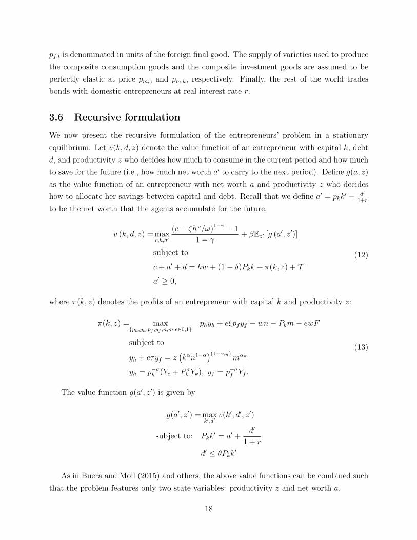
3.6 Recursive formulation

We now present the recursive formulation of the entrepreneurs’ problem in a stationary

equilibrium. Let v(k, d, z) denote the value function of an entrepreneur with capital k, debt

d, and productivity z who decides how much to consume in the current period and how much

to save for the future (i.e., how much net worth a′ to carry to the next period). Define g(a, z)

as the value function of an entrepreneur with net worth a and productivity z who decides

how to allocate her savings between capital and debt. Recall that we define a′ = pkk′ − d′

1+r

to be the net worth that the agents accumulate for the future.

v (k, d, z) = maxc,h,a′

(c− ζhω/ω)1−γ − 1

1− γ+ βEz′ [g (a′, z′)]

subject to

c+ a′ + d = hw + (1− δ)Pkk + π(k, z) + T

a′ ≥ 0,

(12)

where π(k, z) denotes the profits of an entrepreneur with capital k and productivity z:

π(k, z) = max{ph,yh,pf ,yf ,n,m,e∈0,1}

phyh + eξpfyf − wn− Pkm− ewF

subject to

yh + eτyf = z(kαn1−α)(1−αm)

mαm

yh = p−σh (Yc + P σk Yk), yf = p−σf Yf .

(13)

The value function g(a′, z′) is given by

g(a′, z′) = maxk′,d′

v(k′, d′, z′)

subject to: Pkk′ = a′ +

d′

1 + r

d′ ≤ θPkk′

As in Buera and Moll (2015) and others, the above value functions can be combined such

that the problem features only two state variables: productivity z and net worth a.

18

3.7 Stationary Competitive Equilibrium

Let S ≡ A × Z denote the state space of entrepreneurs and let s ∈ S denote an element

of the state space. Let φ denote a measure over S. Assume that pmc and pmk are constant

and given. Then, for a given value of the interest rate r, a recursive stationary compet-

itive equilibrium of this economy consists of aggregate prices {w, ξ, Pk}, policy functions

{d′, k′, e, c, h,m, n, yh, yf , ph, pf , Yc, Yk, ym,c, ym,k}, value functions v and g, and a measure

φ : S → [0, 1] such that the (i) policy and value functions solve the entrepreneurs’ problem;

(ii) policy functions solve the problem of producers of composite consumption goods; (iii)

policy functions solve the problem of producers of composite investment goods; (iv) market

for each variety clears; (v) labor market clears:∫S [n(s) + e(s)F ]φ(s)ds =

∫S h(s)φ(s)ds;

(vi) market for composite consumption good clears:∫S c(s)φ(s)ds = Yc; (vii) market for

composite investment good clears:∫S [x(s) +m(s)]φ(s)ds = Yk; and (viii) measure φ is

stationary.13

4 Mechanism: The role of financial development

In this paper, we investigate the effects of lowering tariffs on imports of investment and

intermediate inputs and the role played by financial development on the magnitude of these

effects. We now describe the mechanism through which this policy affects allocations in our

model, and in the following sections we examine these effects quantitatively.

4.1 Cheaper access to imported production inputs

A unilateral reduction in τk makes imports of intermediate inputs and investment goods

cheaper. This affects the domestic economy through two channels. First, it reduces the

cost of producing the composite investment good. As a result, both materials and capital

become cheaper, decreasing production costs. Second, it leads to a reallocation of demand

by producers of the composite investment goods from domestic to imported varieties. Thus,

a reduction in τk has both positive and negative direct effects on domestic economic activity.

The change in τk also induces general equilibrium effects. As domestic production costs

decline, domestic producers reduce their prices and increase their competitiveness relative to

imports competition, which offsets at least partially the reallocation of demand from domes-

tic to imported varieties by producers of composite investment goods. More importantly,

it also leads producers of composite consumption goods to reallocate their demand from

13See Section 2.5 of the Online Appendix for a more general formal definition of a perfect foresight com-petitive equilibrium that also applies to the transitional dynamics.

19

imported to domestic varieties, as the latter become cheaper when tariffs on production in-

puts are reduced. Thus, total domestic sales are likely to increase. The higher demand for

domestic varieties leads to an increase in the demand for labor and, thus, wages increase.

The increase in wages leads to an increase in labor supply, which further increases domestic

output and investment (since labor and capital are complements). The domestic economy

thus becomes richer when tariffs on imported production inputs are reduced. Finally, the

decline in the price of domestic varieties leads to a lower price of the consumption composite

goods, leading to a real depreciation. This depreciation leads to higher exports and further

increases domestic output.

The gains from a unilateral reduction in τk, however, are not evenly spread across indi-

viduals: exporters, productive and wealthy entrepreneurs benefit directly more from higher

demand for domestic varieties. Yet, these gains are redistributed through several channels.

First, real wages increase in response to the higher demand for domestic varieties, which dis-

proportionately benefits low-productivity and low-net-worth entrepreneurs for whom wages

constitute a higher share of their total income. Second, low-net-worth agents are negatively

affected by the lower tariff revenues, since tariff revenues constitute a higher share of their

income.

Thus, a reduction in tariffs on production inputs leads to increases in consumption and

exports. As a result, it also leads to an economic boom with increased production by

all entrepreneurs. While these gains are unevenly spread across entrepreneurs, there is

substantial redistribution of gains across individuals.

4.2 The role of financial development

Financial development can limit the degree to which the domestic economy benefits from

the forces described above. In an economy with less-developed financial markets (a lower θ),

the pre-liberalization stationary equilibrium is likely to feature a higher share of constrained

entrepreneurs. Thus, as tariffs and production costs are reduced, there is a higher fraction of

entrepreneurs that cannot expand their production as desired, limiting the degree to which

firms can benefit from trade liberalization.

Over time, however, entrepreneurs are able to accumulate funds internally, relaxing their

borrowing constraints and increasing the scale of production closer to their desired level.

Since severely constrained firms have the highest marginal product of capital, these firms

benefit the most from relaxation of their borrowing constraints, which partially offsets the

initial dampening effects of lower financial development.

Furthermore, a lower τk also leads to a reduction in the share of financially constrained ex-

20

porters: The resulting decline in the price of the composite investment good, Pk, effectively

relaxes the borrowing constraint, allowing firms to purchase a higher amount of physical

capital per unit borrowed in financial markets. Thus, this effect further amplifies the pos-

itive impact of the policy change. Again, this effect benefits the most severely constrained

entrepreneurs more and, hence, it is stronger in the less financially developed economy.

The above discussion implies that financial development has an ambiguous impact on

the effect of decreasing tariffs on intermediate inputs and investment goods. On the one

hand, lower financial development tends to dampen the positive direct and indirect effects

of a decrease in τk. On the other hand, it relaxes borrowing constraints, which tends to

strengthen the effects of lowering τk. Determining which effect dominates as well as the

aggregate and distributional effects requires a careful quantitative investigation, which we

perform in the following section.

5 Quantitative analysis

In this section, we investigate quantitatively how financial development affects the aggregate,

distributional, and welfare effects of unilateral trade liberalization that reduces tariffs on

imports of intermediate and capital goods.14

To quantify the role of financial development, we consider a unilateral trade liberalization

as the one that Colombia underwent in the early 1990s. We first calibrate the model to

match key features of Colombian plant-level data, an economy characterized by a low level

of financial development, and then use the model to examine the aggregate effects of a

decrease in import tariffs designed to resemble the one observed in Colombia between 1988

and 1992. We contrast our baseline economy with a counterfactual economy featuring a

high level of financial development (the level of financial development of the U.S. at the

time) but otherwise calibrated to match the same key features of Colombian plant-level

data as in the baseline. We interpret differences in the effects of trade liberalization across

these economies as accounted for by differences in financial development. In particular, we

compare the aggregate, distributional, and welfare effects, both in the long run and along the

transition, between the baseline economy and those implied by the counterfactual economy

with developed financial markets. Finally, we contrast our findings in this section with those

in Section 2 to quantify the extent to which differences in financial development in the model

can account for the differences estimated in the cross-country data.

14We focus on unilateral trade liberalizations motivated by the experience of many developing countriesin the 1990s following the Washington Consensus.

21

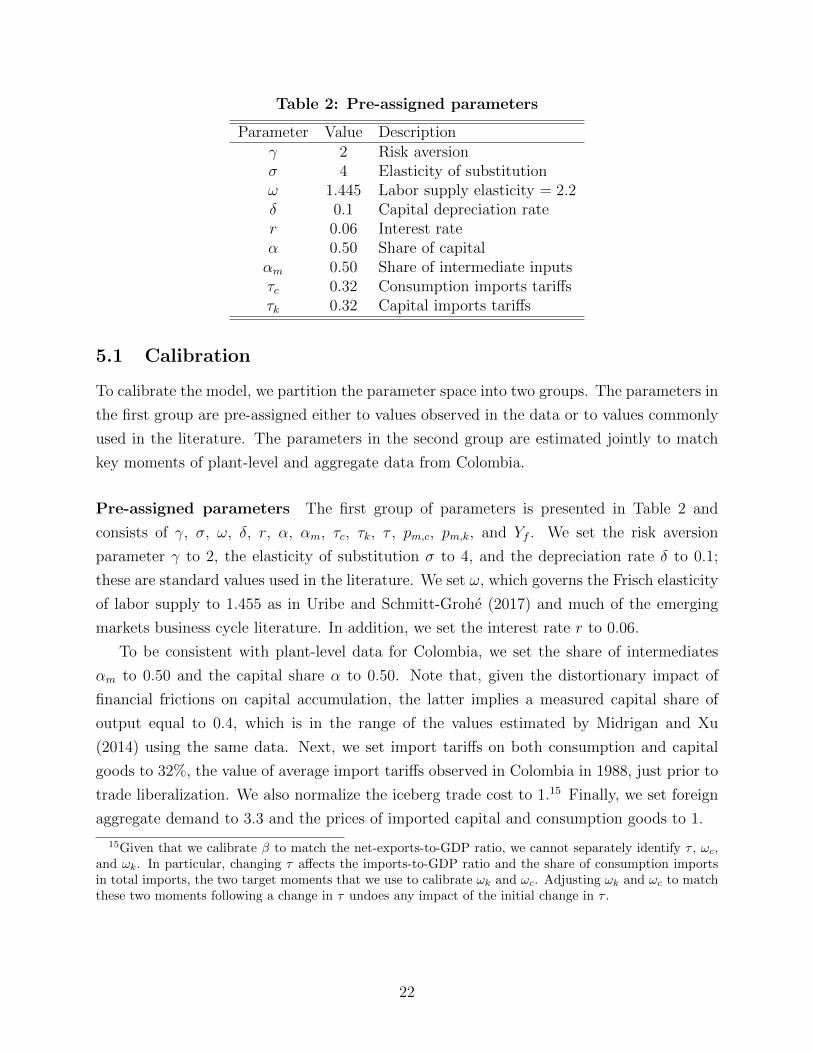
Table 2: Pre-assigned parameters

Parameter Value Descriptionγ 2 Risk aversionσ 4 Elasticity of substitutionω 1.445 Labor supply elasticity = 2.2δ 0.1 Capital depreciation rater 0.06 Interest rateα 0.50 Share of capitalαm 0.50 Share of intermediate inputsτc 0.32 Consumption imports tariffsτk 0.32 Capital imports tariffs

5.1 Calibration

To calibrate the model, we partition the parameter space into two groups. The parameters in

the first group are pre-assigned either to values observed in the data or to values commonly

used in the literature. The parameters in the second group are estimated jointly to match

key moments of plant-level and aggregate data from Colombia.

Pre-assigned parameters The first group of parameters is presented in Table 2 and

consists of γ, σ, ω, δ, r, α, αm, τc, τk, τ , pm,c, pm,k, and Yf . We set the risk aversion

parameter γ to 2, the elasticity of substitution σ to 4, and the depreciation rate δ to 0.1;

these are standard values used in the literature. We set ω, which governs the Frisch elasticity

of labor supply to 1.455 as in Uribe and Schmitt-Grohe (2017) and much of the emerging

markets business cycle literature. In addition, we set the interest rate r to 0.06.

To be consistent with plant-level data for Colombia, we set the share of intermediates

αm to 0.50 and the capital share α to 0.50. Note that, given the distortionary impact of

financial frictions on capital accumulation, the latter implies a measured capital share of

output equal to 0.4, which is in the range of the values estimated by Midrigan and Xu

(2014) using the same data. Next, we set import tariffs on both consumption and capital

goods to 32%, the value of average import tariffs observed in Colombia in 1988, just prior to

trade liberalization. We also normalize the iceberg trade cost to 1.15 Finally, we set foreign

aggregate demand to 3.3 and the prices of imported capital and consumption goods to 1.

15Given that we calibrate β to match the net-exports-to-GDP ratio, we cannot separately identify τ , ωc,and ωk. In particular, changing τ affects the imports-to-GDP ratio and the share of consumption importsin total imports, the two target moments that we use to calibrate ωk and ωc. Adjusting ωk and ωc to matchthese two moments following a change in τ undoes any impact of the initial change in τ .

22

Calibrated parameters The set of calibrated parameters consists of the fixed export

cost, F ; the standard deviation and autocorrelation of the productivity shocks, σε and ρ;

the relative weights of imported goods in the production of investment and consumption

goods, ωk and ωc; the degree of financial development, θ; the discount factor, β; and the

labor weight in preferences, ζ.

To estimate these parameters, we target salient features of both plant-level data from

Colombian manufactures and aggregate data for Colombia. In particular, we use the Annual

Manufacturing Survey, which is collected by the Departamento Administrativo Nacional

de Estadistica (DANE) and surveys all manufacturing plants with at least 10 workers.16

Following Fieler et al. (2018), we use data from 1982 to 1988 to calibrate the model for the

period prior to the tariff reduction implemented in subsequent years. We supplement this

dataset with data from the World Bank.

We choose {F, σε, ρ, ωc, ωk, θ, β, ζ} to match the following moments: (i) the share of

firms that export, (ii) the size of exporters relative to non-exporters (as captured by the

ratio between the average domestic sales of exporters and the average domestic sales of non-

exporters), (iii) the autoregressive coefficient for total sales17, (iv) the share of consumption

goods in imports, (v) the aggregate imports-to-GDP ratio, (vi) the average amount of do-

mestic credit extended to the private sector between 1986 and 1990 as a percentage of GDP

(credit-to-GDP ratio) as reported by the World Bank, and (vii) the net-exports-to-GDP

ratio. Finally, we choose the labor weight in preferences, ζ, such that the aggregate labor

supply is equal to 1 in steady state. We follow the simulated method of moments and choose

these parameters to minimize the squared distance between the moments of the model and

their data counterparts.

Table 3 reports the target moments as well as calibrated parameters and their standard

errors (in parenthesis).18 As observed in the table, our model can match the target moments

closely. Moreover, all parameters are tightly estimated.

Financially developed economy We contrast the baseline economy with a counterfac-

tual economy with developed financial markets. Given our interest in comparing the welfare

implications between these economies, we keep the discount rate unchanged across them;

16These data have been used before by Roberts and Tybout (1997), Ruhl and Willis (2017), and Fieleret al. (2018), among others.

17In the data, we consider firms with all years observed in the sample and estimate the autoregressivecoefficient for total sales with fixed effects.

18We compute standard errors for the parameters as follows. First, we compute standard errors for thetarget moments based on firm-level data via bootstrapping. We draw 100 samples, where each sample ispopulated by 12,347 plants (number of plants in the dataset) drawn with replacement from the originaldataset. Second, for each set of target moments, we re-estimate all the parameters of the model. Finally, wecompute the standard error of each parameter.

23

Table 3: Calibrated parameters – Baseline

Parameter Value Target moment Data ModelF 0.38 Share of exporters 0.11 0.11

(0.013)

σε 0.18 Exporters’ domestic sales premium 5.69 5.69(0.005)

ρ 0.87 Persistence of total sales 0.86 0.86(0.014)

ωc 0.22 Imported consumption / Imports 0.27 0.27(0.001)

ωk 0.30 Imports / GDP 0.12 0.12(0.002)

θ 0.27 Credit / GDP 0.25 0.25(0.003)

β 0.81 Net exports / GDP -0.03 -0.03(0.010)

ζ 0.03 Labor supply in steady state – 1(0.001)

thus, we set β = 0.81, as in the baseline.19 We then estimate F , σ, ρ, ωc, ωk, and θ to match

moments (i)-(vi) described above, except that we now target the average credit-to-GDP ra-

tio between 1986 and 1990 for the U.S., a financially developed economy. Finally we choose

ζ such that the aggregate labor supply is equal to 1 in steady state.20 Thus, examining the

implications of trade liberalization in the counterfactual economy allows us to quantify the

effect that trade liberalization would have had in Colombia had it had the level of financial

development of the U.S. at the time. Table 4 reports the calibrated parameters with their

standard errors and targets for this counterfactual financially developed economy.

5.2 Trade liberalization on intermediate and investment goods

We now investigate the extent to which financial development affects the aggregate dynam-

ics following trade liberalization and its welfare implications. To do so, we contrast our

calibrated baseline and counterfactual economies. We consider the stationary equilibrium of

each of our calibrated models and examine the impact of reducing import tariffs on interme-

diate and capital goods by the magnitudes observed in Colombia between 1988 and 1992. In

19Differences in discount rates would mechanically lead to differences in the welfare effects of trade liber-alization.

20In Section 3.2 of the Online Appendix, we show the effects of trade liberalization in an economy withθ = 0.85 but otherwise with the same parameters as in the baseline economy, isolating the effect of thechange in θ.

24

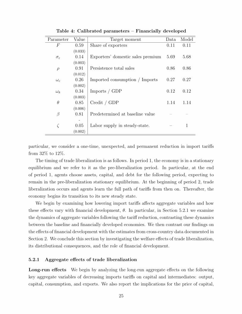
Table 4: Calibrated parameters – Financially developed

Parameter Value Target moment Data ModelF 0.59 Share of exporters 0.11 0.11

(0.033)

σε 0.14 Exporters’ domestic sales premium 5.69 5.68(0.003)

ρ 0.91 Persistence total sales 0.86 0.86(0.012)

ωc 0.26 Imported consumption / Imports 0.27 0.27(0.002)

ωk 0.34 Imports / GDP 0.12 0.12(0.003)

θ 0.85 Credit / GDP 1.14 1.14(0.006)

β 0.81 Predetermined at baseline value – –-

ζ 0.05 Labor supply in steady-state. – 1(0.002)

particular, we consider a one-time, unexpected, and permanent reduction in import tariffs

from 32% to 12%.

The timing of trade liberalization is as follows. In period 1, the economy is in a stationary

equilibrium and we refer to it as the pre-liberalization period. In particular, at the end

of period 1, agents choose assets, capital, and debt for the following period, expecting to

remain in the pre-liberalization stationary equilibrium. At the beginning of period 2, trade

liberalization occurs and agents learn the full path of tariffs from then on. Thereafter, the

economy begins its transition to its new steady state.

We begin by examining how lowering import tariffs affects aggregate variables and how

these effects vary with financial development, θ. In particular, in Section 5.2.1 we examine

the dynamics of aggregate variables following the tariff reduction, contrasting these dynamics

between the baseline and financially developed economies. We then contrast our findings on

the effects of financial development with the estimates from cross-country data documented in

Section 2. We conclude this section by investigating the welfare effects of trade liberalization,

its distributional consequences, and the role of financial development.

5.2.1 Aggregate effects of trade liberalization

Long-run effects We begin by analyzing the long-run aggregate effects on the following

key aggregate variables of decreasing imports tariffs on capital and intermediates: output,

capital, consumption, and exports. We also report the implications for the price of capital,

25

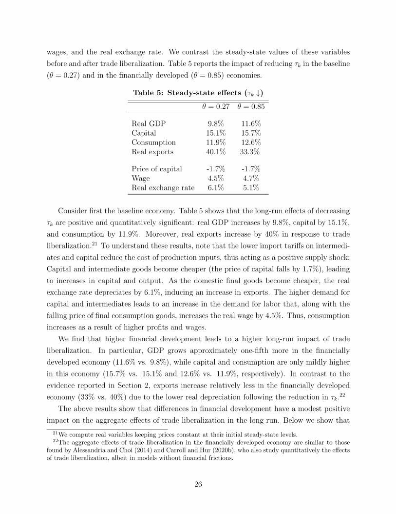
wages, and the real exchange rate. We contrast the steady-state values of these variables

before and after trade liberalization. Table 5 reports the impact of reducing τk in the baseline

(θ = 0.27) and in the financially developed (θ = 0.85) economies.

Table 5: Steady-state effects (τk ↓)

θ = 0.27 θ = 0.85

Real GDP 9.8% 11.6%Capital 15.1% 15.7%Consumption 11.9% 12.6%Real exports 40.1% 33.3%

Price of capital -1.7% -1.7%Wage 4.5% 4.7%Real exchange rate 6.1% 5.1%

Consider first the baseline economy. Table 5 shows that the long-run effects of decreasing

τk are positive and quantitatively significant: real GDP increases by 9.8%, capital by 15.1%,

and consumption by 11.9%. Moreover, real exports increase by 40% in response to trade

liberalization.21 To understand these results, note that the lower import tariffs on intermedi-

ates and capital reduce the cost of production inputs, thus acting as a positive supply shock:

Capital and intermediate goods become cheaper (the price of capital falls by 1.7%), leading

to increases in capital and output. As the domestic final goods become cheaper, the real

exchange rate depreciates by 6.1%, inducing an increase in exports. The higher demand for

capital and intermediates leads to an increase in the demand for labor that, along with the

falling price of final consumption goods, increases the real wage by 4.5%. Thus, consumption

increases as a result of higher profits and wages.

We find that higher financial development leads to a higher long-run impact of trade

liberalization. In particular, GDP grows approximately one-fifth more in the financially

developed economy (11.6% vs. 9.8%), while capital and consumption are only mildly higher

in this economy (15.7% vs. 15.1% and 12.6% vs. 11.9%, respectively). In contrast to the

evidence reported in Section 2, exports increase relatively less in the financially developed

economy (33% vs. 40%) due to the lower real depreciation following the reduction in τk.22

The above results show that differences in financial development have a modest positive

impact on the aggregate effects of trade liberalization in the long run. Below we show that

21We compute real variables keeping prices constant at their initial steady-state levels.22The aggregate effects of trade liberalization in the financially developed economy are similar to those

found by Alessandria and Choi (2014) and Carroll and Hur (2020b), who also study quantitatively the effectsof trade liberalization, albeit in models without financial frictions.

26

these results mask large differences in aggregate outcomes along the transition as well as

substantial differences in welfare gains.

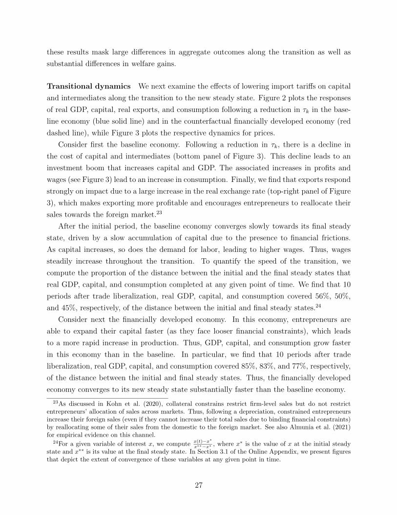
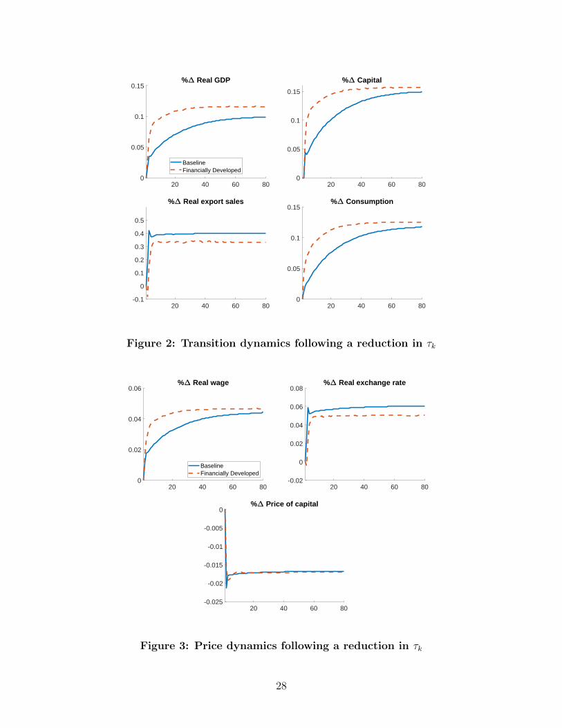
Transitional dynamics We next examine the effects of lowering import tariffs on capital

and intermediates along the transition to the new steady state. Figure 2 plots the responses

of real GDP, capital, real exports, and consumption following a reduction in τk in the base-

line economy (blue solid line) and in the counterfactual financially developed economy (red

dashed line), while Figure 3 plots the respective dynamics for prices.

Consider first the baseline economy. Following a reduction in τk, there is a decline in

the cost of capital and intermediates (bottom panel of Figure 3). This decline leads to an

investment boom that increases capital and GDP. The associated increases in profits and

wages (see Figure 3) lead to an increase in consumption. Finally, we find that exports respond

strongly on impact due to a large increase in the real exchange rate (top-right panel of Figure

3), which makes exporting more profitable and encourages entrepreneurs to reallocate their

sales towards the foreign market.23

After the initial period, the baseline economy converges slowly towards its final steady

state, driven by a slow accumulation of capital due to the presence to financial frictions.

As capital increases, so does the demand for labor, leading to higher wages. Thus, wages

steadily increase throughout the transition. To quantify the speed of the transition, we

compute the proportion of the distance between the initial and the final steady states that

real GDP, capital, and consumption completed at any given point of time. We find that 10

periods after trade liberalization, real GDP, capital, and consumption covered 56%, 50%,

and 45%, respectively, of the distance between the initial and final steady states.24

Consider next the financially developed economy. In this economy, entrepreneurs are

able to expand their capital faster (as they face looser financial constraints), which leads

to a more rapid increase in production. Thus, GDP, capital, and consumption grow faster

in this economy than in the baseline. In particular, we find that 10 periods after trade

liberalization, real GDP, capital, and consumption covered 85%, 83%, and 77%, respectively,

of the distance between the initial and final steady states. Thus, the financially developed

economy converges to its new steady state substantially faster than the baseline economy.

23As discussed in Kohn et al. (2020), collateral constrains restrict firm-level sales but do not restrictentrepreneurs’ allocation of sales across markets. Thus, following a depreciation, constrained entrepreneursincrease their foreign sales (even if they cannot increase their total sales due to binding financial constraints)by reallocating some of their sales from the domestic to the foreign market. See also Almunia et al. (2021)for empirical evidence on this channel.

24For a given variable of interest x, we compute x(t)−x∗

x∗∗−x∗ , where x∗ is the value of x at the initial steadystate and x∗∗ is its value at the final steady state. In Section 3.1 of the Online Appendix, we present figuresthat depict the extent of convergence of these variables at any given point in time.

27

20 40 60 800

0.05

0.1

0.15% Real GDP

BaselineFinancially Developed

20 40 60 800

0.05

0.1

0.15

% Capital

20 40 60 80-0.1

0

0.1

0.2

0.3

0.4

0.5

% Real export sales

20 40 60 800

0.05

0.1

0.15% Consumption

Figure 2: Transition dynamics following a reduction in τk

20 40 60 800

0.02

0.04

0.06% Real wage

BaselineFinancially Developed

20 40 60 80-0.02

0

0.02

0.04

0.06

0.08% Real exchange rate

20 40 60 80-0.025

-0.02

-0.015

-0.01

-0.005

0% Price of capital

Figure 3: Price dynamics following a reduction in τk

28

We thus conclude that financial frictions significantly slow down the adjustment to a

reduction in tariffs on imports of intermediates and capital. In the next subsection, we show

that these findings are consistent with the cross-country differences in aggregate dynamics

following trade liberalization as documented in Section 2, suggesting frictions in financial

markets play a significant role in accounting for these patterns.

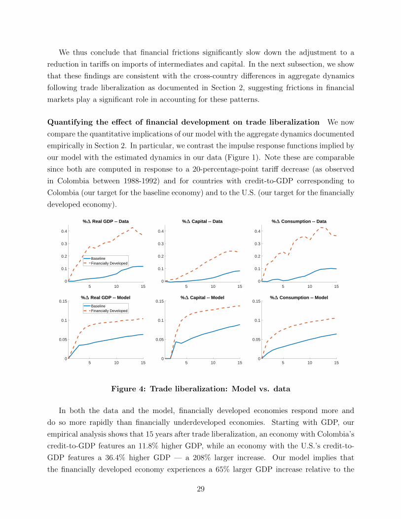
Quantifying the effect of financial development on trade liberalization We now

compare the quantitative implications of our model with the aggregate dynamics documented

empirically in Section 2. In particular, we contrast the impulse response functions implied by

our model with the estimated dynamics in our data (Figure 1). Note these are comparable

since both are computed in response to a 20-percentage-point tariff decrease (as observed

in Colombia between 1988-1992) and for countries with credit-to-GDP corresponding to

Colombia (our target for the baseline economy) and to the U.S. (our target for the financially

developed economy).

5 10 150

0.1

0.2

0.3

0.4

% Real GDP -- Data

BaselineFinancially Developed

5 10 150

0.1

0.2

0.3

0.4

% Capital -- Data

5 10 150

0.1

0.2

0.3

0.4

% Consumption -- Data

5 10 150

0.05

0.1

0.15% Real GDP -- Model

BaselineFinancially Developed

5 10 150

0.05

0.1

0.15% Capital -- Model

5 10 150

0.05

0.1

0.15% Consumption -- Model

Figure 4: Trade liberalization: Model vs. data

In both the data and the model, financially developed economies respond more and

do so more rapidly than financially underdeveloped economies. Starting with GDP, our

empirical analysis shows that 15 years after trade liberalization, an economy with Colombia’s

credit-to-GDP features an 11.8% higher GDP, while an economy with the U.S.’s credit-to-

GDP features a 36.4% higher GDP — a 208% larger increase. Our model implies that

the financially developed economy experiences a 65% larger GDP increase relative to the

29

financially underdeveloped economy. Overall, our model can explain 16.5% of the difference

estimated in the data in the responses between the two economies in the first 15 years

following trade liberalization.25

We obtain similar conclusions from contrasting the dynamics of consumption and capi-

tal implied by the model with those estimated in the data. Our empirical analysis implies

that consumption would have increased by 9.8% in the financially underdeveloped economy

and 36.0% in the financially developed economy, while our model’s respective implications

are 6.4% and 10.5%. Overall, the model explains 16.5% of the difference in consumption

responses between the two economies in the first 15 years following trade liberalization.

Finally, our empirical analysis implies that capital increases by 8.3% in the financially un-

derdeveloped and 22.7% in the financially developed economy over the same period. The

respective increases implied by the model are 8.8% and 13.8%. When accounting for the

first 15 years following the trade liberalization, the model explains 45.6% of the difference

in the dynamics of capital between the two economies.

These results show that, for the 15 years following trade liberalization, the model explains

between 17% (in the cases of GDP and consumption) to 46% (in the case of capital) of

the observed differences between the financially developed and underdeveloped economies.

Some of the differences in the estimated responses of the economies to trade liberalization

could be related to other factors that we are not able to account for in the regressions: For

example, some of these countries may have experienced exogenous capital inflows or financial

liberalization jointly with trade liberalization, or may have benefited from reduced tariffs by

their trade partners. In Section 6, we revisit our findings in a quantitative analysis that

incorporates other shocks during the transition, to match the aggregate dynamics observed

in Colombia, accounting for some of the factors omitted in this section.

Trade liberalization on all imports It is useful to compare the effects of trade lib-

eralization on intermediate and capital goods to the effects of trade liberalization on all

imports, including consumption goods. As we show in Section 3.4 of the Online Appendix,

the effects of reducing tariffs on all imports have similar effects as reducing tariffs only on

intermediate and capital goods. In the baseline economy, following a decrease in τc and τk

from 32% to 12%, in the long run, GDP increases by 9.4%, capital by 14.6%, consump-

tion by 11.8%, and real exports by 48.8%. Thus, except for exports, aggregate variables

increase by less than when only tariffs to investment goods are reduced: A decrease in τc has

a contractionary effect on domestic economy because cheaper consumption imports crowd

25To compute this value, we compare the area between the lines corresponding to the change in GDP inthe financially developed and financially underdeveloped economies in the model with the analogous areaimplied by our regressions.

30

out domestic production.26 Similar effects shape the dynamics in the financially developed

economy. However, we find that the speed of transition to the new steady state following

decreases in τc and τk is very similar to the one observed following a decrease in only τk.

Therefore, our results suggest that most of the aggregate effects from trade liberalization are

accounted for by tariffs on intermediate and capital goods.

5.2.2 Welfare and distributional effects

In this section, we analyze how financial development affects the welfare gains from trade

liberalization, both in the aggregate and across the distribution of agents. To compute

aggregate gains we use a “consumption-equivalent” welfare measure. That is, we ask how

much agents’ consumption would have to increase in the pre-liberalization steadystate to

make them indifferent between the economy without trade liberalization and the one with

lower tariffs examined above. Thus, our approach is similar to the one followed by Brooks

and Dovis (2020) and Carroll and Hur (2020b).27

Formally, let vg0(s) be the value function of an entrepreneur in state s in the initial steady

state when its consumption has been increased by g percent forever. That is,

vg0(k, d, z) = U((1 + g)c∗0(s), h∗0(s)) + βE[vg0(k∗′0 , d∗′0 , z

′)], (14)

where c∗0, h∗0, k∗0, and d∗0 are entrepreneurs’ optimal consumption, labor supply, capital, and

debt choices in the initial steady state. Note that when g = 0, vg0 is simply the value

function in the initial steady state. Recall that we defined s = {k, d, z} to be the vector of

entrepreneurs’ states and S to be the state space. To compute aggregate welfare gains, we

solve for g such that ∫Svg0(s)φ0(s)ds =

∫SvT (s)φ0(s)ds, (15)

where φ0(s) is the initial steady state’s stationary measure and vT (s) is the value function

of an entrepreneur in state s in period 2 right after trade liberalization.

Similarly, we compute the welfare gains for a group of entrepreneurs whose state just

before the trade liberalization belonged to a subset S0 of the state space (for example,

26See Sections 3.3 and 3.4 of the Online Appendix for more details.27It should be pointed out that our model assumes a particular ownership structure of firms where each

household owns exactly one firm. This assumption is standard in the literature that studies welfare in theenvironments with heterogeneous firms (see, for example, Buera and Shin (2011), Moll (2014), or Tetenyi(2021)).

31

exporters and non-exporters) and we solve for g such that∫S0vg0(s)φ0(s)ds =

∫S0vT (s)φ0(s)ds, (16)

As mentioned above, the above measures of welfare gains are standard in the literature.

However, in a model with heterogeneous firms, alternative way to measure gains from trade

liberalization is to compute change sin present discounted value (PDV) of firms’ profits. In

Section 4 of the Online Appendix, we report results using that measure, which are qualita-

tively similar to those reported below.

Aggregate welfare We focus first on aggregate welfare gains. Table 6 presents our find-

ings. The first row reports the welfare gains from trade liberalization as defined in Equation

(15). The second row reports the welfare gains excluding the transition — that is, restricting

attention to the comparison between the initial and final steady states. Thus, comparing

the first and second rows allows us to evaluate the welfare cost of the transition.

Table 6: ∆Welfare (τk ↓)

θ = 0.27 θ = 0.85Overall 0.5% 3.0%Excluding transition 5.8% 5.8%

The first row of Table 6 shows that the welfare gains from trade liberalization are much

lower in the economy with financial frictions: only 0.5% compared to 3.0% in the financially

developed economy. Thus, low financial development substantially limits the welfare gains

from a reduction in tariffs on capital and intermediates.

The second row of Table 6 instead shows that if economies could immediately adjust to

their final steady states, then welfare would increase by 5.8% in both economies. That is,

not only would welfare increase much more in both economies in the absence of the slow

transition due to financial frictions, but gains would be the same across the two economies.

This finding indicates that the difference in welfare gains between the two economies is fully

accounted for by the faster transition to the final steady state in the financially developed

economy.

Welfare distribution To better understand the heterogeneous welfare gains from trade

liberalization, we next investigate how welfare gains vary across different subsets of en-

trepreneurs and across the joint distribution of assets and productivity.

32

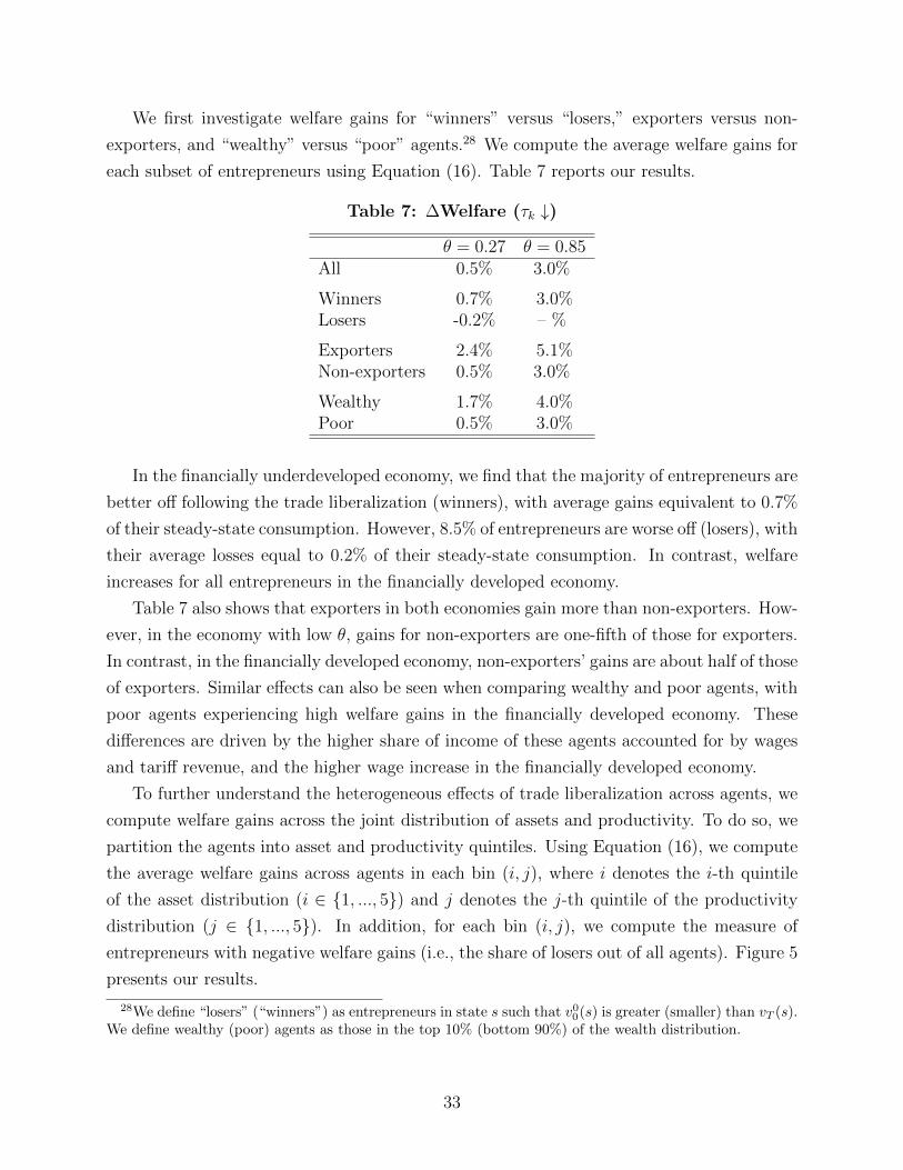
We first investigate welfare gains for “winners” versus “losers,” exporters versus non-

exporters, and “wealthy” versus “poor” agents.28 We compute the average welfare gains for

each subset of entrepreneurs using Equation (16). Table 7 reports our results.

Table 7: ∆Welfare (τk ↓)

θ = 0.27 θ = 0.85All 0.5% 3.0%

Winners 0.7% 3.0%Losers -0.2% – %

Exporters 2.4% 5.1%Non-exporters 0.5% 3.0%

Wealthy 1.7% 4.0%Poor 0.5% 3.0%

In the financially underdeveloped economy, we find that the majority of entrepreneurs are

better off following the trade liberalization (winners), with average gains equivalent to 0.7%

of their steady-state consumption. However, 8.5% of entrepreneurs are worse off (losers), with

their average losses equal to 0.2% of their steady-state consumption. In contrast, welfare

increases for all entrepreneurs in the financially developed economy.

Table 7 also shows that exporters in both economies gain more than non-exporters. How-

ever, in the economy with low θ, gains for non-exporters are one-fifth of those for exporters.

In contrast, in the financially developed economy, non-exporters’ gains are about half of those

of exporters. Similar effects can also be seen when comparing wealthy and poor agents, with

poor agents experiencing high welfare gains in the financially developed economy. These

differences are driven by the higher share of income of these agents accounted for by wages

and tariff revenue, and the higher wage increase in the financially developed economy.

To further understand the heterogeneous effects of trade liberalization across agents, we

compute welfare gains across the joint distribution of assets and productivity. To do so, we

partition the agents into asset and productivity quintiles. Using Equation (16), we compute

the average welfare gains across agents in each bin (i, j), where i denotes the i-th quintile

of the asset distribution (i ∈ {1, ..., 5}) and j denotes the j-th quintile of the productivity

distribution (j ∈ {1, ..., 5}). In addition, for each bin (i, j), we compute the measure of

entrepreneurs with negative welfare gains (i.e., the share of losers out of all agents). Figure 5

presents our results.

28We define “losers” (“winners”) as entrepreneurs in state s such that v00(s) is greater (smaller) than vT (s).We define wealthy (poor) agents as those in the top 10% (bottom 90%) of the wealth distribution.

33

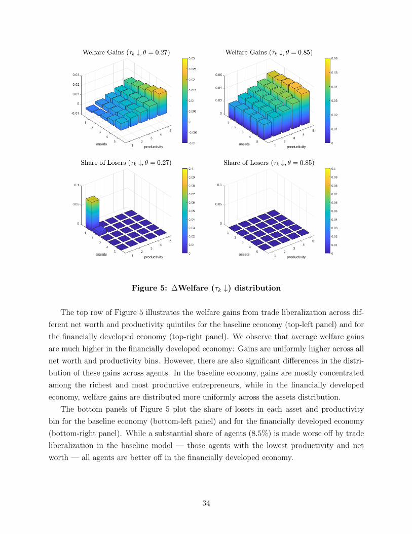
12

34

5

productivity

12

34

5assets

0

0.05

0.1

0

0.01

0.02

0.03

0.04

0.05

0.06

0.07

0.08

0.09

0.1

Figure 5: ∆Welfare (τk ↓) distribution

The top row of Figure 5 illustrates the welfare gains from trade liberalization across dif-

ferent net worth and productivity quintiles for the baseline economy (top-left panel) and for

the financially developed economy (top-right panel). We observe that average welfare gains

are much higher in the financially developed economy: Gains are uniformly higher across all

net worth and productivity bins. However, there are also significant differences in the distri-

bution of these gains across agents. In the baseline economy, gains are mostly concentrated

among the richest and most productive entrepreneurs, while in the financially developed

economy, welfare gains are distributed more uniformly across the assets distribution.

The bottom panels of Figure 5 plot the share of losers in each asset and productivity

bin for the baseline economy (bottom-left panel) and for the financially developed economy

(bottom-right panel). While a substantial share of agents (8.5%) is made worse off by trade

liberalization in the baseline model — those agents with the lowest productivity and net

worth — all agents are better off in the financially developed economy.

34

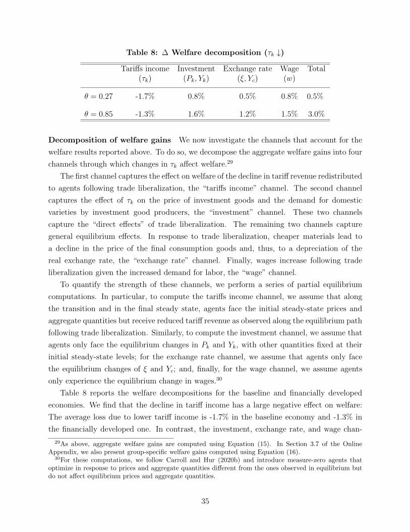
Table 8: ∆ Welfare decomposition (τk ↓)

Tariffs income Investment Exchange rate Wage Total(τk) (Pk, Yk) (ξ, Yc) (w)

θ = 0.27 -1.7% 0.8% 0.5% 0.8% 0.5%

θ = 0.85 -1.3% 1.6% 1.2% 1.5% 3.0%

Decomposition of welfare gains We now investigate the channels that account for the

welfare results reported above. To do so, we decompose the aggregate welfare gains into four

channels through which changes in τk affect welfare.29

The first channel captures the effect on welfare of the decline in tariff revenue redistributed

to agents following trade liberalization, the “tariffs income” channel. The second channel

captures the effect of τk on the price of investment goods and the demand for domestic

varieties by investment good producers, the “investment” channel. These two channels

capture the “direct effects” of trade liberalization. The remaining two channels capture

general equilibrium effects. In response to trade liberalization, cheaper materials lead to

a decline in the price of the final consumption goods and, thus, to a depreciation of the

real exchange rate, the “exchange rate” channel. Finally, wages increase following trade

liberalization given the increased demand for labor, the “wage” channel.

To quantify the strength of these channels, we perform a series of partial equilibrium

computations. In particular, to compute the tariffs income channel, we assume that along

the transition and in the final steady state, agents face the initial steady-state prices and

aggregate quantities but receive reduced tariff revenue as observed along the equilibrium path

following trade liberalization. Similarly, to compute the investment channel, we assume that

agents only face the equilibrium changes in Pk and Yk, with other quantities fixed at their

initial steady-state levels; for the exchange rate channel, we assume that agents only face

the equilibrium changes of ξ and Yc; and, finally, for the wage channel, we assume agents

only experience the equilibrium change in wages.30

Table 8 reports the welfare decompositions for the baseline and financially developed

economies. We find that the decline in tariff income has a large negative effect on welfare:

The average loss due to lower tariff income is -1.7% in the baseline economy and -1.3% in

the financially developed one. In contrast, the investment, exchange rate, and wage chan-

29As above, aggregate welfare gains are computed using Equation (15). In Section 3.7 of the OnlineAppendix, we also present group-specific welfare gains computed using Equation (16).

30For these computations, we follow Carroll and Hur (2020b) and introduce measure-zero agents thatoptimize in response to prices and aggregate quantities different from the ones observed in equilibrium butdo not affect equilibrium prices and aggregate quantities.

35

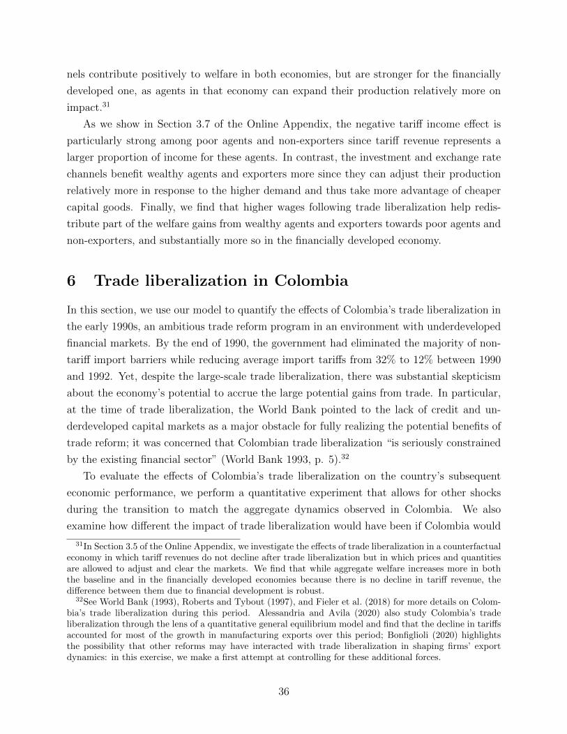
nels contribute positively to welfare in both economies, but are stronger for the financially

developed one, as agents in that economy can expand their production relatively more on

impact.31

As we show in Section 3.7 of the Online Appendix, the negative tariff income effect is

particularly strong among poor agents and non-exporters since tariff revenue represents a

larger proportion of income for these agents. In contrast, the investment and exchange rate

channels benefit wealthy agents and exporters more since they can adjust their production

relatively more in response to the higher demand and thus take more advantage of cheaper

capital goods. Finally, we find that higher wages following trade liberalization help redis-

tribute part of the welfare gains from wealthy agents and exporters towards poor agents and

non-exporters, and substantially more so in the financially developed economy.

6 Trade liberalization in Colombia

In this section, we use our model to quantify the effects of Colombia’s trade liberalization in

the early 1990s, an ambitious trade reform program in an environment with underdeveloped

financial markets. By the end of 1990, the government had eliminated the majority of non-

tariff import barriers while reducing average import tariffs from 32% to 12% between 1990

and 1992. Yet, despite the large-scale trade liberalization, there was substantial skepticism

about the economy’s potential to accrue the large potential gains from trade. In particular,

at the time of trade liberalization, the World Bank pointed to the lack of credit and un-

derdeveloped capital markets as a major obstacle for fully realizing the potential benefits of

trade reform; it was concerned that Colombian trade liberalization “is seriously constrained

by the existing financial sector” (World Bank 1993, p. 5).32

To evaluate the effects of Colombia’s trade liberalization on the country’s subsequent

economic performance, we perform a quantitative experiment that allows for other shocks

during the transition to match the aggregate dynamics observed in Colombia. We also

examine how different the impact of trade liberalization would have been if Colombia would

31In Section 3.5 of the Online Appendix, we investigate the effects of trade liberalization in a counterfactualeconomy in which tariff revenues do not decline after trade liberalization but in which prices and quantitiesare allowed to adjust and clear the markets. We find that while aggregate welfare increases more in boththe baseline and in the financially developed economies because there is no decline in tariff revenue, thedifference between them due to financial development is robust.

32See World Bank (1993), Roberts and Tybout (1997), and Fieler et al. (2018) for more details on Colom-bia’s trade liberalization during this period. Alessandria and Avila (2020) also study Colombia’s tradeliberalization through the lens of a quantitative general equilibrium model and find that the decline in tariffsaccounted for most of the growth in manufacturing exports over this period; Bonfiglioli (2020) highlightsthe possibility that other reforms may have interacted with trade liberalization in shaping firms’ exportdynamics: in this exercise, we make a first attempt at controlling for these additional forces.

36

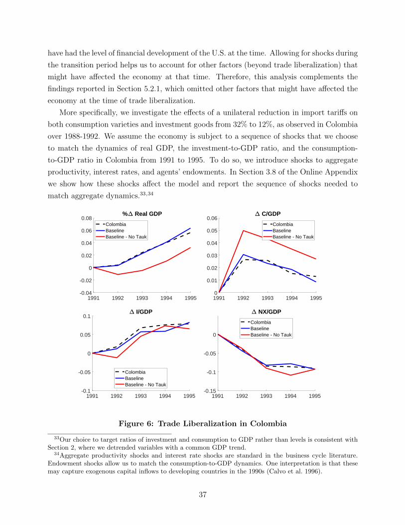
have had the level of financial development of the U.S. at the time. Allowing for shocks during

the transition period helps us to account for other factors (beyond trade liberalization) that

might have affected the economy at that time. Therefore, this analysis complements the

findings reported in Section 5.2.1, which omitted other factors that might have affected the

economy at the time of trade liberalization.

More specifically, we investigate the effects of a unilateral reduction in import tariffs on

both consumption varieties and investment goods from 32% to 12%, as observed in Colombia

over 1988-1992. We assume the economy is subject to a sequence of shocks that we choose

to match the dynamics of real GDP, the investment-to-GDP ratio, and the consumption-

to-GDP ratio in Colombia from 1991 to 1995. To do so, we introduce shocks to aggregate

productivity, interest rates, and agents’ endowments. In Section 3.8 of the Online Appendix

we show how these shocks affect the model and report the sequence of shocks needed to

match aggregate dynamics.33,34

1991 1992 1993 1994 1995-0.04

-0.02

0

0.02

0.04

0.06

0.08% Real GDP

ColombiaBaselineBaseline - No Tauk

1991 1992 1993 1994 19950

0.01

0.02

0.03

0.04

0.05

0.06 C/GDP

ColombiaBaselineBaseline - No Tauk

1991 1992 1993 1994 1995-0.1

-0.05

0

0.05

0.1 I/GDP

ColombiaBaselineBaseline - No Tauk

1991 1992 1993 1994 1995-0.15

-0.1

-0.05

0

NX/GDP

ColombiaBaselineBaseline - No Tauk

Figure 6: Trade Liberalization in Colombia

33Our choice to target ratios of investment and consumption to GDP rather than levels is consistent withSection 2, where we detrended variables with a common GDP trend.

34Aggregate productivity shocks and interest rate shocks are standard in the business cycle literature.Endowment shocks allow us to match the consumption-to-GDP dynamics. One interpretation is that thesemay capture exogenous capital inflows to developing countries in the 1990s (Calvo et al. 1996).

37

Figure 6 depicts the dynamics following trade liberalization of GDP, consumption-to-

GDP, investment-to-GDP, and net-exports-to-GDP for Colombia (black dashed line), the

baseline model (blue solid line), and a counterfactual experiment with the same shocks but

no reduction in tariffs on capital and intermediate goods (red solid line). Thus, the difference

between the blue and red solid lines captures the effects of trade liberalization on capital

and intermediate goods.

Figure 6 shows that Colombia’s trade liberalization explains a sizable portion of the

growth between 1991 and 1995: The tariff decrease explains 3.1 percentage points of the 5.7-

percentage-point growth in detrended GDP by 1995 (55% of the observed growth). Trade

liberalization also led to lower consumption-to-GDP, higher investment-to-GDP and lower

net-exports-to-GDP.35

We then perform an analogous exercise for our financially developed economy. Recall

that this is an economy calibrated to feature the level of credit-to-GDP of the U.S. but that

otherwise targets the same moments as in the baseline economy. In the same spirit, we

estimate an alternative sequence of shocks chosen to target the aggregate dynamics observed

in Colombia between 1991 and 1995. Figure 7 shows the effects of financial development

(the difference between the blue and red solid lines in Figure 6) on GDP, consumption-to-

GDP, investment-to-GDP, and net-exports-to-GDP for the baseline and for the financially

developed economies.36

As shown in Figure 7, if Colombia would have had the level of financial development of the

U.S., trade liberalization would have induced an increase of 7.7 percentage points in GDP

by 1995 — more than twice the 3.1 percentage points implied by our baseline economy.

Moreover, there would have been a much larger boom in investment and implied trade

deficit. Our findings confirm the results in Section 5: In response to trade liberalization,

GDP, consumption, and capital increase more in financially developed economies.

7 Conclusions

In this paper, we study the role of financial development on the aggregate effects and welfare

implications of reducing international trade barriers on capital and intermediate inputs. We

set up a quantitative general equilibrium model with heterogeneous firms subject to financial

constraints, estimate it to match salient features from Colombian plant-level data, and find

that the adjustment to trade liberalization is significantly slower in financially underdevel-

35Notice that lower consumption-to-GDP does not imply lower consumption but instead that consumptionincreased by less than GDP over this period as a consequence of trade liberalization.

36In Section 3.8 of the Online Appendix, we show an analogous figure to Figure 6 for the financiallydeveloped economy.

38

1991 1992 1993 1994 19950

0.02

0.04

0.06

0.08% Real GDP - Tauk Liberalization

BaselineFinancially Developed

1991 1992 1993 1994 1995-0.03

-0.025

-0.02

-0.015

-0.01

-0.005

0 C/GDP - Tauk Liberalization

BaselineFinancially Developed

1991 1992 1993 1994 1995-0.02

0

0.02

0.04

0.06

0.08

0.1 I/GDP - Tauk Liberalization

BaselineFinancially Developed

1991 1992 1993 1994 1995-0.1

-0.05

0

0.05

0.1 NX/GDP - Tauk Liberalization

BaselineFinancially Developed

Figure 7: Trade Liberalization in Colombia – Financially Developed

oped economies. Moreover, we find that financial development increases the welfare gains

from trade liberalization: Low-income agents benefit from higher wages, while exporters

benefit from a depreciated real exchange rate and lower capital costs.

Our paper contributes to the literature along three dimensions. First, we document that

financially underdeveloped economies grow relatively slower than their financially developed

counterparts after trade liberalization: 15 years after trade liberalization, GDP, consumption,

and capital are 25% to 40% larger on average across financially developed economies vs.

approximately 10% larger on average in economies with weaker financial development. Our

second contribution is to use a general equilibrium model to quantify the extent to which

these cross-country differences in aggregate dynamics are accounted for just by financial

development: we find that between 16% to 44% of the observed differences can be explained

by financial development alone. Our third contribution is to investigate the implications

of these findings for both aggregate welfare as well as for the distribution of welfare gains

across various population subgroups: we find that welfare gains in the financially developed

economy are six times higher than in the financially underdeveloped economy (3.0% versus

0.5%).

39

More broadly, our findings provide a rationale for the resistance to trade liberalization

in less-developed economies: There might be less to gain from trade openness in these

economies, particularly in the short and medium run. Therefore, our results imply that

trade liberalization might need to be pursued together with reforms aimed towards improving

firms’ access to external finance.

References

Alessandria, G. and O. Avila, “Trade integration in colombia: a dynamic general equilibrium studywith new exporter dynamics,” Journal of Economic Dynamics and Control 115 (2020), 103871.

Alessandria, G. and H. Choi, “Establishment Heterogeneity, Exporter Dynamics, and the Effects ofTrade Liberalization,” Journal of International Economics 94 (2014), 207–223.

Almunia, M., P. Antras, D. Lopez-Rodriguez and E. Morales, “Venting out: Exports during adomestic slump,” American Economic Review 111 (2021), 3611–62.

Amiti, M. and J. Konings, “Trade liberalization, intermediate inputs, and productivity: Evidence fromIndonesia,” American Economic Review 97 (2007), 1611–1638.

Anderson, J. E., M. Larch and Y. V. Yotov, “Growth and trade with frictions: A structural estimationframework,” Technical Report, National Bureau of Economic Research, 2015.

Asturias, J., S. Hur, T. J. Kehoe and K. J. Ruhl, “The interaction and sequencing of policy reforms,”Journal of Economic Dynamics and Control 72 (2016), 45–66.

Autor, D. H., D. Dorn and G. H. Hanson, “The China shock: Learning from labor-market adjustmentto large changes in trade,” Annual Review of Economics 8 (2016), 205–240.

Autor, D. H., D. Dorn, G. H. Hanson and J. Song, “Trade adjustment: Worker-level evidence,”Quarterly Journal of Economics 129 (2014), 1799–1860.

Bonfiglioli, A., “Comment on “Trade integration in Colombia: A dynamic general equilibrium study withnew exporter dynamics”,” Journal of Economic Dynamics and Control 115 (2020), 103872.

Brooks, W. and A. Dovis, “Credit market frictions and trade liberalizations,” Journal of MonetaryEconomics 111 (2020), 32–47.

Buera, F. J., J. P. Kaboski and Y. Shin, “Finance and Development: A Tale of Two Sectors,” AmericanEconomic Review 101 (2011), 1964–2002.

Buera, F. J. and B. Moll, “Aggregate Implications of a Credit Crunch,” American Economic Journal:Macro 7 (2015).

Buera, F. J. and Y. Shin, “Self-insurance vs. self-financing: A welfare analysis of the persistence ofshocks,” Journal of Economic Theory 146 (2011), 845–862.

Caggese, A. and V. Cunat, “Financing Constraints, Firm Dynamics, Export Decisions, and AggregateProductivity,” Review of Economic Dynamics 16 (January 2013), 177–193.

Calvo, G. A., L. Leiderman and C. M. Reinhart, “Inflows of Capital to Developing Countries in the1990s,” Journal of Economic Perspectives 10 (1996), 123–139.

Carroll, D. and S. Hur, “On the distributional effects of international tariffs,” Working Paper, 2020a.Carroll, D. R. and S. Hur, “On the heterogeneous welfare gains and losses from trade,” Journal of

Monetary Economics 109 (2020b), 1–16.Chaney, T., “Liquidity constrained exporters,” Journal of Economic Dynamics and Control 72 (2016),

141–154.Cihak, M., A. Demirguc-Kunt, E. Feyen and R. Levine, “Benchmarking financial systems around

the world,” The World Bank (2012).Do, Q.-T. and A. A. Levchenko, “Comparative advantage, demand for external finance, and financial

development,” Journal of Financial Economics 86 (2007), 796–834.Estevadeordal, A. and A. M. Taylor, “Is the Washington consensus dead? Growth, openness, and

the great liberalization, 1970s–2000s,” Review of Economics and Statistics 95 (2013), 1669–1690.Feenstra, R. C., R. Inklaar and M. P. Timmer, “The next generation of the Penn World Table,”

American Economic Review 105 (2015), 3150–82.

40

Fieler, A. C., M. Eslava and D. Y. Xu, “Trade, quality upgrading, and input linkages: Theory andevidence from Colombia,” American Economic Review 108 (2018), 109–46.

Goldberg, P., A. Khandelwal, N. Pavcnik and P. Topalova, “Trade liberalization and new importedinputs,” American Economic Review 99 (2009), 494–500.

Greenwood, J., Z. Hercowitz and G. W. Huffman, “Investment, capacity utilization, and the realbusiness cycle,” The American Economic Review (1988), 402–417.

Irwin, D. A., “Does Trade Reform Promote Economic Growth? A Review of Recent Evidence,” TechnicalReport, National Bureau of Economic Research, 2019.

King, R. G. and R. Levine, “Finance and growth: Schumpeter might be right,” Quarterly Journal ofEconomics 108 (1993), 717–737.

Kohn, D., F. Leibovici and M. Szkup, “Financial Frictions and New Exporter Dynamics,” InternationalEconomic Review 57 (2016), 453–486.

———, “Financial frictions and export dynamics in large devaluations,” Journal of International Economics122 (2020), 103257.

———, “Financial Frictions and International Trade: A Review,” Oxford Research Encyclopedia of Eco-nomics and Finance (2022).

Leibovici, F., “Financial development and international trade,” Journal of Political Economy 129 (2021),3405–3446.

Manova, K., “Credit Constraints and the Adjustment to Trade Reform,” in The Costs of Adjustment toTrade Reform (World Bank Trade and Development Series, Palgrave Macmillan, 2010).

———, “Credit Constraints, Heterogeneous Firms, and International Trade,” Review of Economic Studies80 (April 2013), 711–744.

Melitz, M. J., “The Impact of Trade on Intra-Industry Reallocations and Aggregate Industry Productiv-ity,” Econometrica 71 (November 2003), 1695–1725.

Midrigan, V. and D. Y. Xu, “Finance and Misallocation: Evidence from Plant-Level Data,” AmericanEconomic Review 104 (November 2014), 422–58.

Moll, B., “Productivity Losses from Financial Frictions: Can Self-Financing Undo Capital Misallocation?,”American Economic Review 104 (2014), 3186–3221.

Pavcnik, N., “Trade Liberalization, Exit, and Productivity Improvements: Evidence from Chilean Plants,”Review of Economic Studies 69 (2002), 245–276.

Ravikumar, B., A. M. Santacreu and M. Sposi, “Capital accumulation and dynamic gains from trade,”Journal of International Economics 119 (2019), 93–110.

Roberts, M. J. and J. R. Tybout, “The Decision to Export in Colombia: An Empirical Model of Entrywith Sunk Costs,” American Economic Review 87 (1997), 545–564.

Ruhl, K. J. and J. L. Willis, “New exporter dynamics,” International Economic Review 58 (2017),703–726.

Sachs, J. D., A. Warner, A. Aslund and S. Fischer, “Economic reform and the process of globalintegration,” Brookings Papers on Economic Activity 1995 (1995), 1–118.

Saffie, F., L. Varela and K.-M. Yi, “The Micro and Macro Dynamics of Capital Flows,” TechnicalReport, National Bureau of Economic Research, 2020.

Tetenyi, L., “Trade, misallocation, and capital market integration,” Working Paper, 2021.Topalova, P. and A. Khandelwal, “Trade liberalization and firm productivity: The case of India,”

Review of Economics and Statistics 93 (2011), 995–1009.Uribe, M. and S. Schmitt-Grohe, Open Economy Macroeconomics (Princeton University Press, 2017).Wacziarg, R. and K. H. Welch, “Trade liberalization and growth: New evidence,” World Bank Economic

Review 22 (2008), 187–231.World Bank, “Colombia - Export Development Project (English),” Technical Report, Washington, DC:

World Bank, 1993.

41