NBER WORKING PAPER SERIES

FINANCIAL DEVELOPMENT AND THE CHOICE OF TRADE PARTNERS

Man Lung ChanKalina Manova

Working Paper 18867http://www.nber.org/papers/w18867

NATIONAL BUREAU OF ECONOMIC RESEARCH1050 Massachusetts Avenue

Cambridge, MA 02138March 2013

I declare that I have no relevant or material financial interests that relate to the research described inthis paper. The views expressed herein are those of the authors and do not necessarily reflect the viewsof the National Bureau of Economic Research.

NBER working papers are circulated for discussion and comment purposes. They have not been peer-reviewed or been subject to the review by the NBER Board of Directors that accompanies officialNBER publications.

© 2013 by Man Lung Chan and Kalina Manova. All rights reserved. Short sections of text, not to exceedtwo paragraphs, may be quoted without explicit permission provided that full credit, including © notice,is given to the source.

Financial Development and the Choice of Trade PartnersMan Lung Chan and Kalina ManovaNBER Working Paper No. 18867March 2013, Revised March 2015JEL No. F10,F14,F36,G20

ABSTRACT

What determines the choice of countries' trade partners? We show theoretically and empirically thatfinancial market imperfections affect the number and identity of exporters' destinations. Bigger economieswith lower trade costs are more attractive markets because they offer higher export profits. This generatesa pecking order of destinations such that firms serve all countries above a cut-off level of market potential.Credit constraints, however, raise this cut-off above the first best. Financially advanced nations thushave more trade partners and go further down the pecking order, especially in sectors that rely heavilyon the financial system. Our results provide new, systematic evidence that countries follow a hierarchyof export destinations, that market size and trade costs determine this hierarchy, and that financialfrictions interact importantly with it. This has policy implications for the effects of cross-border linkagesthat depend on the number and identity of countries' trade partners.

Man Lung ChanPh.D. CandidateDepartment of EconomicsStanford University579 Serra MallStanford, CA 94305jmlchan@stanford.edu

Kalina ManovaDepartment of EconomicsStanford University579 Serra MallStanford, CA 94305and NBERmanova@stanford.edu

1 Introduction

For many developing countries, international trade contributes significantly to aggregate output and

economic growth. Exporting provides access to a bigger consumer market, enabling firms to expand

production, increase domestic employment and reap higher profits. This can in turn boost firms’ pro-

ductivity by allowing them to benefit from scale economies under existing manufacturing practices, as

well as to invest in innovation and technology upgrading. The very exposure to international know-how

and the frequent use of imported inputs in production for foreign countries can mediate productivity

spillovers across borders. Aside from raising income levels and growth rates, exporting can also reduce

volatility over time. By diversifying across multiple consumer markets, exporters may be able to hedge

fluctuations in country-specific demand and insure against downturns at home.

These arguments suggest that being able to not only export more, but also to sell to more destinations

matters for aggregate welfare. In practice, successful economies indeed boast high exports to many

destinations. For example, countries with more trade partners in 1985 exported substantially more over

the next 10 years (Figure 1). They attained faster average annual growth in both exports and GDP per

capita (Figures 2a and 2b). They also experienced less volatility, as reflected in lower standard deviations

of these growth rates over time (Figures 3a and 3b). As the regressions in Appendix Table 1 show, these

correlations are not driven by cross-country differences in initial export volumes in 1985. While faster

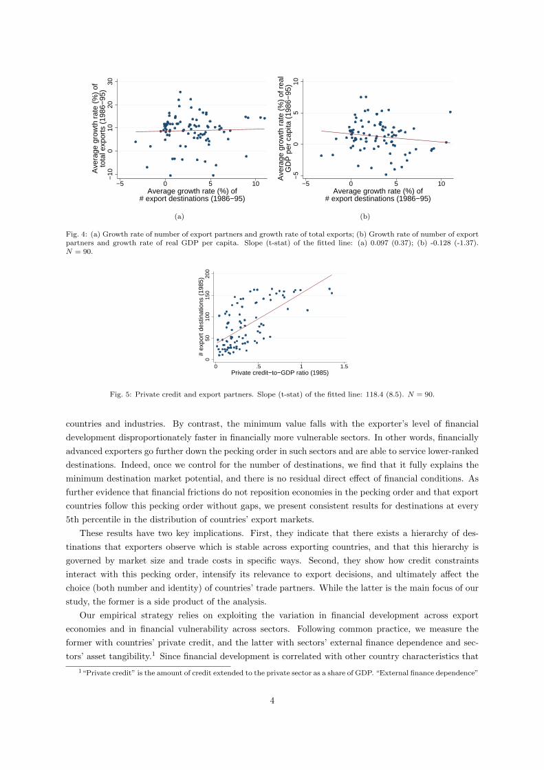
growth in the number of export destinations is not associated with faster income or export growth in the

raw data (Figures 4a and 4b), it is when catch-up effects are taken into account in regressions controlling

for initial trade activity (Appendix Table 1).

These patterns indicate that it is important to understand what determines countries’ ability to estab-

lish more trade links. Among other things, financial development appears strongly positively correlated

with exporters’ destination count (Figure 5).

This paper examines the effect of financial market imperfections on the number and characteristics of

exporters’ trade partners. Because market size and trade costs vary across countries, bigger economies

with lower trade costs are relatively more profitable export targets. This generates a pecking order of

destinations based on their market potential. In the absence of credit constraints, firms export to all

destinations above a cut-off level of market potential. Financial frictions, however, raise this cut-off

and prevent firms from serving some markets that they would otherwise have entered in the first best.

Financially developed nations thus have more trade partners and go further down the pecking order of

destinations, especially in sectors that rely more heavily on the financial system.

We study these questions formally by extending the theory developed in Manova (2013). In the

model, heterogeneous firms incur trade costs in each market they enter. They face liquidity problems

and require outside funding for a fraction of these costs, which they can raise by pledging collateral.

Financial contracts are imperfectly enforced and creditors face default risks. Producers are thus unable to

pursue all profitable export opportunities because they have limited access to capital. Instead, companies

optimally add destinations in decreasing order of profitability until they exhaust their financial resources.

Aggregating across firms, this implies that credit constraints restrict countries’ number of trade partners

to suboptimal levels and change the composition of these trade partners.

The theory illustrates how these distortions vary systematically across exporting countries and sectors.

The strength of financial contractibility depends on how developed the exporter’s financial institutions

are. Firms’ need for external finance and availability of collateralizable assets differ across industries for

technological reasons, exogenous from the perspective of individual producers. Hence while all countries

can export to the most attractive destinations in the world, financially advanced countries also sell to

2

1015

20

(log)

Tot

al e

xpor

ts(1

986−

95 m

ean)

0 50 100 150 200# export destinations (1985)

Fig. 1: Export partners and total exports. Slope (t-stat) of the fitted line: 0.047 (23.1). N = 90.

−10

010

2030

Ave

rage

gro

wth

rat

e (%

) of

tota

l exp

orts

(19

86−

95)

0 50 100 150 200# export destinations (1985)

(a)

−5

05

10

Ave

rage

gro

wth

rat

e (%

) of

rea

lG

DP

per

cap

ita (

1986

−95

)

0 50 100 150 200# export destinations (1985)

(b)

Fig. 2: (a) Export partners and growth rate of total exports; (b) Export partners and growth rate of GDP per capita.Slope (t-stat) of the fitted line: (a) 0.054 (4.2); (b) 0.018 (3.8). N = 90.

11.

52

2.5

Std

dev

of g

row

th r

ate

(%)

ofto

tal e

xpor

ts (

1986

−95

)

0 50 100 150 200# export destinations (1985)

(a)

11.

051.

11.

151.

21.

25

Std

dev

of g

row

th r

ate

(%)

of r

eal

GD

P p

er c

apita

(19

86−

95)

0 50 100 150 200# export destinations (1985)

(b)

Fig. 3: (a) Export partners and std. dev. of growth rate of total exports; (b) Export partners and std. dev. of growthrate of GDP per capita. Slope (t-stat) of the fitted line: (a) -0.003 (-6.2); (b) -0.0003 (-4.6). N = 90.

economies with less market potential. Importantly, these effects are more pronounced in sectors that

require more external capital and in sectors that are endowed with fewer tangible assets.

We provide strong empirical support for these predictions using panel data on bilateral trade for 78

export countries and 27 industries in 1985-1995. We first derive model-consistent estimating equations

that relate characteristics of an exporter’s destination countries to its number of destinations and credit

conditions at home. We then develop a model-consistent ranking of destinations by market potential,

and record the highest and lowest destination market potential among an exporter’s trade partners.

In line with the theory, we document no systematic variation in the maximum value across export

3

−10

010

2030

Ave

rage

gro

wth

rat

e (%

) of

tota

l exp

orts

(19

86−

95)

−5 0 5 10Average growth rate (%) of

# export destinations (1986−95)

(a)

−5

05

10

Ave

rage

gro

wth

rat

e (%

) of

rea

lG

DP

per

cap

ita (

1986

−95

)

−5 0 5 10Average growth rate (%) of

# export destinations (1986−95)

(b)

Fig. 4: (a) Growth rate of number of export partners and growth rate of total exports; (b) Growth rate of number of exportpartners and growth rate of real GDP per capita. Slope (t-stat) of the fitted line: (a) 0.097 (0.37); (b) -0.128 (-1.37).N = 90.

050

100

150

200

# ex

port

des

tinat

ions

(19

85)

0 .5 1 1.5Private credit−to−GDP ratio (1985)

Fig. 5: Private credit and export partners. Slope (t-stat) of the fitted line: 118.4 (8.5). N = 90.

countries and industries. By contrast, the minimum value falls with the exporter’s level of financial

development disproportionately faster in financially more vulnerable sectors. In other words, financially

advanced exporters go further down the pecking order in such sectors and are able to service lower-ranked

destinations. Indeed, once we control for the number of destinations, we find that it fully explains the

minimum destination market potential, and there is no residual direct effect of financial conditions. As

further evidence that financial frictions do not reposition economies in the pecking order and that export

countries follow this pecking order without gaps, we present consistent results for destinations at every

5th percentile in the distribution of countries’ export markets.

These results have two key implications. First, they indicate that there exists a hierarchy of des-

tinations that exporters observe which is stable across exporting countries, and that this hierarchy is

governed by market size and trade costs in specific ways. Second, they show how credit constraints

interact with this pecking order, intensify its relevance to export decisions, and ultimately affect the

choice (both number and identity) of countries’ trade partners. While the latter is the main focus of our

study, the former is a side product of the analysis.

Our empirical strategy relies on exploiting the variation in financial development across export

economies and in financial vulnerability across sectors. Following common practice, we measure the

former with countries’ private credit, and the latter with sectors’ external finance dependence and sec-

tors’ asset tangibility.1 Since financial development is correlated with other country characteristics that

1“Private credit” is the amount of credit extended to the private sector as a share of GDP. “External finance dependence”

4

could influence export activity, interpreting its direct effect as causal is problematic. It can also become

theoretically ambiguous in general equilibrium. On the other hand, the differential effect of financial

development across industries survives in general equilibrium and cannot easily be attributed to alter-

native explanations. For this reason, this difference-in-difference approach has been widely used in the

literature as a means of establishing a causal effect of credit constraints on various economic outcomes.

It permits the inclusion of a rigorous set of control variables such as Heckscher-Ohlin sources of compar-

ative advantage, country and sector fixed effects. We further ensure that our results do not capture the

role of overall development or other institutions by controlling for the interactions of GDP per capita,

rule of law and corruption with the sector measures of financial vulnerability.

We propose two methodologies to gauge destinations’ relative position in the pecking order. We

first examine different proxies for market size and trade costs as the sole determinants of destinations’

desirability. We then pursue an alternative approach, which remains agnostic about the exact drivers

of market potential and is based on the principle of revealed preferences: If a market is particularly

attractive and profitable, more exporters will enter it. The number of nations selling to a given country

thus implicitly signals its market potential. By the same logic, we also adopt a semi-structural two-

stage estimation technique. In the first stage, we run a probit regression of an indicator for positive

bilateral exports on exporter, importer and sector fixed effects. We use the coefficients on the importer

dummies from this regression as an index of market desirability in the second stage. We find robust

results consistent with the model’s predictions both with the direct and with the agnostic measures of

market potential.

Our findings extend three lines of research in the prior literature. We advance a large literature that

seeks to understand why the incidence and magnitude of cross-border transactions varies substantially

across countries, sectors and firms. At the aggregate level, about half of all country pairs conduct no

bilateral trade, and another 15% initiate only one-way flows (Helpman et al. 2008). At the micro level,

export sales are highly concentrated in a few large and productive firms that ship to many countries

(Bernard et al. 2007). These patterns can be explained if economies differ in their market potential and

exporters observe a pecking order of destinations. While recent work-horse models of international trade

incorporate this feature, however, they can have opposing implications as to which country characteristics

determine market potential and how. For example, bigger destinations rank higher in the pecking order

in Melitz (2003), but lower in Melitz and Ottaviano (2008) and Eaton and Kortum (2002). Separately,

Armenter and Koren (2014) present a random-assignment model of “balls” (i.e. export transactions) to

“bins” (i.e. export markets), in which a pecking order arises atheoretically, rather than because firms

purposefully add destinations in decreasing order of profitability.

Despite this theoretical interest, the pecking order hypothesis has received little attention in the

empirical literature to date, with mixed results. Eaton et al. (2011a) show that French companies with

more export destinations tend to enter less popular markets, i.e. countries served by fewer manufacturers.

However, there are significant deviations from a uniform pecking order across firms, which Eaton et al.

(2011a) rationalize with idiosyncratic firm-destination specific export cost and demand draws. In cross-

country data, Helpman et al. (2008) find that bigger market sizes and lower trade costs increase the

probability of bilateral trade on average, but do not examine whether exporting countries observe a

hierarchy of destinations without gaps. It has thus remained an open empirical question whether there is

a stable pecking order of exporting at the aggregate level and what factors govern it. Our analysis is one

of the first to provide systematic evidence that countries do follow a (common) hierarchy of destinations,

is the share of capital expenditures not financed from internal cash flows from operations. “Asset tangibility” is the shareof plant, property and equipment in total assets. See Section 4 for more details.

5

that bigger market size and lower trade costs raise destinations in this hierarchy, and that financial

frictions interact nontrivially with it.2 In the process, we develop a methodology for obtaining agnostic,

comprehensive measures of market potential from observable data that can be applied to other contexts,

such as testing models with and without a pecking order of products within multi-product firms (e.g.

Bernard et al. 2011, Dhingra 2013, Mayer et al. 2014).

Most directly, this paper adds to the growing body of work at the intersection of international trade

and corporate finance (c.f. Foley and Manova forthcoming). A number of theoretical models have

examined the mechanisms through which credit constraints disrupt trade activity (e.g. Manova 2013,

Feenstra et al. forthcoming). These frameworks have illustrated that financially developed countries have

a comparative advantage in financially vulnerable sectors. They have also emphasized the heterogeneous

impact of imperfect capital markets across firms. On the empirical side, evidence indicates that credit

constraints impede firms’ export operations and distort aggregate trade flows, both in normal times and

during crisis episodes (e.g. Berman and Hericourt 2010, Amiti and Weinstein 2011, Minetti and Zhu

2011, Chor and Manova 2012, Bricongne et al. 2012, Manova 2013, Feenstra et al. forthcoming).

Our contribution to this literature is in identifying a novel dimension of global commerce that is

affected by credit market imperfections: the choice of countries’ trade partners. Of note, Manova (2013)

establishes theoretically and empirically that (i) financially developed countries export to more desti-

nations in financially more vulnerable sectors. We complement this result by showing theoretically and

empirically that (ii) financial development operates by allowing exporting nations to go further down

the pecking order of destinations. Importantly, while our theoretical predictions follow directly from the

Manova (2013) framework which we extend, our empirical findings are not automatically implied by hers

because pattern (i) can obtain in alternative trade models with financial frictions that do not generate

pattern (ii). What guarantees (ii) is that credit constraints do not change the ranking of destinations in

the pecking order and do not cause gaps in the order in which destinations are added. These features

are, however, sensitive to modeling assumptions about the economic environment and the nature of fi-

nancial frictions (see Section 2.4). Hence our analysis implicitly provides validation for the theoretical

mechanisms we propose in favor of alternative models. This may shed light on the potential welfare

losses from imperfect capital markets if greater deviations from the first-best choice of trade partners is

associated with lower gains from trade.

More broadly, our work is motivated by and informs studies that relate international trade linkages

to economic growth, cross-country technology spillovers, and contagion. Trade openness is typically

associated with faster income growth, although results are somewhat mixed (Rodrik 2005). Countries’

number of trade partners too appears positively correlated with growth after controlling for other co-

variates (Kali et al. 2007, Figure 2). Evidence also suggests that access to imported inputs allows firms

in developing countries to improve product quality and to manufacture more products (Verhoogen 2008,

Goldberg et al. 2010, Manova and Zhang 2012). In addition, firms in developing economies appear to

learn from exporting and experience productivity gains when selling to developed nations (de Loecker

2007). Separately, business cycles are more synchronized between countries that trade with each other

(Frankel and Rose 1998, Clark and van Wincoop 2001, Baxter and Kouparitsas 2005). Moreover, cost

or demand shocks originating in one economy tend to propagate to its trade partners (Burstein et al.

2008, Eaton et al. 2011b).

The effects of these cross-country interdependencies clearly hinge on the identity of the economies in

2In work subsequent to ours, Muuls (2008) has confirmed that our results for the maximum and minimum GDP acrossan exporter’s destinations hold not only in aggregate, but also at the firm level: Financially healthier firms in Belgium areable to export to smaller destinations than credit constrained firms.

6

question in terms of their size, average income, overall development, TFP, and role in global financial

and goods markets. Understanding these interdependencies can thus be enhanced by better understand-

ing how countries’ trade partners are determined. Our results highlight the importance of financial

development and credit constraints as one such determinant.

The remainder of the paper is organized as follows. The next section outlines the theoretical frame-

work, while Section 3 derives model-consistent estimating equations. We introduce the data in Section

4 and present the empirical results in Section 5. The last section concludes.

2 Theoretical framework

We extend the Manova (2013) theoretical model to study how financial market imperfections affect

the choice of countries’ trade partners. We provide a variant of that model here, focusing specifically

on the predictions for the pecking order of export destinations. The underlying production and market

structure follows Melitz (2003) in a static, partial-equilibrium set-up. Correspondingly, the exposition

moves quickly and refers the reader to Manova (2013) for further details.

2.1 Set up

The world consists of I countries and S sectors. Within each country and sector, a continuum of

heterogeneous firms produce differentiated goods. The representative consumer in country i has utility

Ui =∏s C

θsis , where Cis =

[∫ω∈Ωis

qis(ω)αdω] 1α

, Ωis spans the set of available varieties, and θs gives the

share of expenditure on industry s. The constant elasticity of substitution across products is given by

ε = 1/(1− α) > 1 with 0 < α < 1. Demand for variety ω in sector s is thus qis(ω) = pis(ω)−εθsYiP 1−εis

, where

pis(ω) is the price of that variety, Yi equals total spending in country i, and Pis = [∫ω∈Ωis

pis(ω)1−εdω]1

1−ε

reflects an ideal price index.

2.2 Firms’ export behavior

Firms in country j pay a sunk cost cjsej in order to enter industry s. At that point, they draw

their productivity level 1/a from a cumulative distribution function G(a) with support [aL, aH ], aH >

aL > 0. This productivity draw uniquely determines manufacturers’ production and trade behavior.

The marginal cost of making one unit of output is cjsa, where cjs is the country-sector specific cost

of a cost-minimizing bundle of inputs. Exporting to market i entails fixed (cjsfij > 0) and variable

trade costs of the iceberg variety (τij > 1) in each period of trading.3 These costs could, for example,

relate to researching consumer demand, building and maintaining foreign distribution networks, product

customization, and transportation. Setting τjj = 1 would correspond to operations in the domestic

market. Given our interest, we concentrate on companies’ export decisions. In other words, we study

the selection of domestic producers into exporting, and leave the selection of entrants into domestic

production in the background.

3We allow the fixed costs of firm entry and exporting to depend on factor costs in the exporting country to add richnessand flexibility to the model. Intuitively, the fixed investment required to establish a new firm is bigger when local factorinputs are more expensive, for example because that raises the cost of building a plant, hiring managers, buying equipment,conducting research and product development etc. Likewise, fixed trade costs may be higher when the workers employedin marketing research, product customization or advertising are more expensive. This formulation is not consequential forthe model’s predictions since fixed costs enter all relevant expressions linearly and are additively separable.

7

Firms face liquidity needs because a portion ds ∈ (0, 1) of the fixed trade cost is incurred up-front and

cannot be financed with retained earnings or internal cash flows from operations.4 In order to raise these

funds in the external capital market, companies must pledge collateral. Their available collateralizable

assets constitute a fraction ts ∈ (0, 1) of the initial entry cost, which can be interpreted as tangible

investments in plant, property, and equipment. Financially more vulnerable sectors have relatively

higher ds and lower ts.

Entrepreneurs obtain outside financing by making a take-it-or-leave-it offer to potential (risk-neutral)

investors. However, agents operate in an environment with imperfect contractibility. With an exogenous

probability λj ∈ (0, 1), financial agreements are enforced and lenders are repaid a pre-specified amount

Fjs(a). Otherwise, with probability (1 − λj), the firm defaults, and the creditor claims the collateral

tscjsej . Manufacturers then have to replace this collateral to continue operations in the future. The

parameter λj can thus be thought of as an indicator of the strength of financial institutions or the level

of financial development in exporting country j.

Profit-maximizing exporters choose which destination markets i to enter, the optimal price pijs and

quantity qijs in each destination, and the terms of the financial contract they propose to investors (total

loan size, repayment Fjs(a), and collateral posted tscjsej).5 If TP (a) is the set of trade partners that

a firm with productivity 1/a sells to, the firm’s total liquidity needs will amount to∑i∈TP (a) dscjsfij .

The company’s maximization problem can therefore be expressed as follows:

maxTP,p,q,F

πjs(a) =∑

i∈TP (a)

pijs(a)qijs(a)− qijs(a)τijcjsa− (1− ds)cjsfij − λjFjs(a)− (1− λj)tscjsej

(2.1)

s.t. (1) qijs(a) =pijs(a)−εθsYi

P 1−εis

,

(2) Ajs(a) ≡∑

i∈TP (a)

pijs(a)qijs(a)− qijs(a)τijcjsa− (1− ds)cjsfij ≥ Fjs(a), and

(3) Bjs(a) ≡ −∑

i∈TP (a)

dscjsfij + λjFjs(a) + (1− λj)tscjsej ≥ 0.

The expression for profits reflects the fact that the firm finances all of its variable costs qijs(a)τijcjsa

and a fraction (1−ds) of its fixed costs internally, pays the investor Fjs(a) when the contract is enforced

(with probability λj), and replaces the collateral in case of default (with probability (1− λj)). In the

absence of financial frictions, exporters maximize profits subject to demand (1). With liquidity needs,

two additional conditions bind manufacturers’ decisions. In case of repayment, entrepreneurs can offer

at most their net revenues to the creditor, i.e. Ajs(a) ≥ Fjs(a). Also, investors only fund the company

if their net return Bjs (a) exceeds their outside option, here normalized to 0.

With competitive credit markets, lenders always break even in expectation. This implies that pro-

ducers adjust their payment Fjs(a) so as to bring the financier to his participation constraint in (3), i.e.

Bjs (a) = 0. The optimization problem therefore reduces to a familiar Melitz-type formulation with the

4While requiring firms to use external finance for part of their variable costs would not qualitatively affect our predic-tions, securing funding for fixed trade costs is plausibly more difficult than raising funds for their working capital needsassociated with variable trade costs. For example, banks often provide letters of credit to cover the latter since these aretied to specific trade transactions and the goods shipped can serve as collateral themselves.

5To maximize their chance of obtaining the loan, it is in firms’ interest to pledge all of their collateralizable assets.

8

additional credit constraint (2):

maxTP,p,q

πjs(a) =∑

i∈TP (a)

pijs(a)qijs(a)− qijs(a)τijcjsa− cjsfij =∑

i∈TP (a)

πijs(a) (2.2)

s.t. (1) qijs(a) =pijs(a)−εθsYi

P 1−εis

, and

(2) Ajs(a) ≥ 1

λj

∑i∈TP (a)

dscjsfij − (1− λj)tscjsej

.

The profits πijs(a) from any market are unaffected by financial considerations (conditional on ex-

porting there). This occurs because firms require external capital only for their fixed costs. They thus

optimally set the same price and quantity in every destination they choose to serve as in the absence of

financial frictions. Incorporating the demand condition (1), the maximization problem finally becomes:

maxTP

πjs(a) =∑

i∈TP (a)

(1− α)

(τijcjsa

αPis

)1−ε

θsYi − cjsfij

=

∑i∈TP (a)

πijs(a) (2.3)

s.t.∑

i∈TP (a)

(1− α)

(τijcjsa

αPis

)1−ε

θsYi − cjsfij

≥ 1− λj

λj

∑i∈TP (a)

dscjsfij − tscjsej

.

We build intuition for the solution to this problem in steps. Note first that profitability will vary

across export markets. From the perspective of firms in country j and sector s, destinations i can be

uniquely ranked in terms of their relative profitability: While profits πijs(a) increase with productivity

1/a, one can verify that πxjs(a′) > πyjs(a

′) whenever πxjs(a) > πyjs(a). In other words, if destination

x is more profitable than destination y for firm a, it is also more desirable for firm a′, if both firms are

based in the same country j and sector s.

Observe also that importing countries with a larger market size Yi and lower trade costs, τij and fij ,

are more attractive because they guarantee higher profits. We jointly refer to these characteristics as

market potential (MP), and to the ranking of destinations in decreasing order of market potential as the

pecking order. A summary statistic for the market potential of destination i relevant for firms exporting

from country j is MPijs = Yi/(τijfij). What matters for our purposes is not the exact functional form

for MPijs, but rather that it is increasing in Yi and decreasing in τij and fij .

In this set-up, all firms in a given country j will observe the same pecking order regardless of their

sector affiliation, since the pertinent sector characteristics (cjs, θs, ds and ts) enter separably. We capture

these characteristics with sector fixed effects in our empirical analysis. To the extent that the hierarchy of

destinations in fact varies across industries within j, the theoretical predictions below would be weakened

and we would be less likely to find support for them in the data.

On the other hand, our framework does not guarantee that manufacturers in different export countries

will follow the same pecking order. While all firms exporting to i face the same destination market size

Yi regardless of their country of origin j, they incur different bilateral trade costs τij and fij that depend

on the country pair. If these trade costs are separable into exporter- and importer-specific components,

then the pecking order will be stable across exporting nations. For example, if τij = τiτj and fij = fifj ,

then the summary statistic for market potential can be expressed as MPijs = MPi = Yi/(τifi) for all j.

We return to this point later on.

With perfect financial contractibility (λj = 1), each firm would export to all countries that promise

9

non-negative profits. For a firm with productivity 1/a, there will be a minimum level of market potential

such that the firm serves all destinations more attractive than it. This threshold is pinned down by

πijs(a) = 0. We denote this first-best group of trade partners TPFB(a), and the number of countries in

it #TPFB(a).

With financial frictions (λj < 1), entrepreneurs might have to forgo exporting to some countries in

their ideal set TPFB(a). This arises because each destination not only brings extra profits, but also

imposes additional liquidity needs. The limited collateral a firm possesses, however, constrains the total

loan it can access. This implies that the marginal country the producer ships to will have to generate

strictly positive profits to warrant the extra burden it places on the overall financial contract. We restrict

our attention to the interesting case when the total loan size needed to access all destinations in TPFB(a)

exceeds the value of the available collateral, i.e.,∑i∈TPFB(a) dscjsfij > tscjsej .

Formally, the exporter’s constrained optimal choice of trade partners TP ∗(a) satisfies:

∑i∈TP∗(a)

πijs(a) ≥ 1− λjλj

∑i∈TP∗(a)

dscjsfij − tscjsej

and

∑i∈TP∗(a)+1

πijs(a) <1− λjλj

∑i∈TP∗(a)+1

dscjsfij − tscjsej

, (2.4)

where the set TP ∗(a)+1 includes all countries in TP ∗(a) plus the destination ranked next in the pecking

order according to its market potential.

By construction, #TP ∗(a) ≤ #TPFB(a) necessarily holds. #TP ∗(a) will be strictly below the

first-best #TPFB(a) whenever∑i∈TPFB(a) πijs(a) <

1−λjλj

∑i∈TPFB(a) dscjsfij − tscjsej

, i.e. when

the profits from exporting to all destinations in the first-best set∑i∈TPFB(a) πijs(a) are insufficient to

incentivize investors to provide the necessary funding∑i∈TPFB(a) dscjsfij given the available collateral

tscjsej and probability of repayment λj . Note that the left-hand side of this inequality (i.e. global firm

profits) rises monotonically with productivity, while the right-hand side is invariant across firms. This

implies that more productive firms will be able to go further down the pecking order and export to more

destinations. Moreover, only companies below a certain productivity level will be affected by financial

concerns and forced to reduce their number of trade partners below the first best.

2.3 Countries’ trade partners

We next consider the implications of imperfect financial markets for countries’ aggregate export

behavior. All producers target destinations in decreasing order of market potential and follow the same

pecking order (for given exporter-sector characteristics). In the aggregate, country j will therefore export

to country i in sector s as long as at least one firm in j can afford to do so. This will in turn depend

on importer i’s position in j’s hierarchy of destinations. For example, if i is the fifth most attractive

market, at least one firm in j should sell to five or more nations in order to ship to i; if i is ranked tenth,

at least one firm should serve ten or more markets; etc. This implies a one-to-one mapping between the

number of country j’s trade partners #TPjs and the identity of these trade partners.

For any given set (number) of export destinations TPjs (#TPjs), there is a minimum productivity

level 1/aTPjs above which firms can sustain this many trade links. This cut-off is determined by the

10

liquidity constraint in equation (2.3):

∑i∈TPjs

(1− α)

(τijcjsaTPjs

αPis

)1−ε

θsYi − cjsfij

=

1− λjλj

∑i∈TPjs

dscjsfij − tscjsej

. (2.5)

The left-hand side of this equality is increasing in the productivity cut-off. Taking derivatives, simple

comparative statics describe the effect of financial market imperfections on the right-hand side RHS:

∂RHS

∂λj= − 1

λ2j

∑i∈TPjs

dscjsfij − tscjsej

< 0,

∂RHS

∂ds=

1− λjλj

∑i∈TPjs

cjsfij > 0,∂RHS

∂ts= −1− λj

λjcjsej < 0, (2.6)

∂2RHS

∂λj∂ds= − 1

λ2j

∑i∈TPjs

cjsfij < 0,∂2RHS

∂λj∂ts=

1

λ2j

cjsej > 0.

This immediately implies that the productivity cut-off for exporting from j to #TPjs destinations is

higher in sectors that require more external finance or have fewer tangible assets,∂(1/aTPjs)

∂ds> 0 and

∂(1/aTPjs)∂ts

< 0. The threshold also falls with the strength of financial contractibility,∂(1/aTPjs)

∂λj< 0.

Importantly, financial development reduces the export cut-off relatively more in financially vulnerable

industries,∂2(1/aTPjs)∂λj∂ds

< 0 and∂2(1/aTPjs)∂λj∂ts

> 0.6 If no firm in country j has productivity above this

cut-off (i.e., if 1/aTPjs > 1/aL), then j will sell to fewer than #TPjs markets and will certainly not

export to the destination country in position #TPjs of j’s pecking order.

Recall that the ranking of destinations by market potential will generally vary across exporting

nations because it depends on bilateral trade costs. Ceteris paribus, these comparative statics therefore

describe the impact of financial development on trade patterns within an exporting country over time

and across sectors. To the extent that the pecking order is universal, they would also apply to the

cross-sectional variation across exporting nations and sectors. Our empirical exercise takes this into

account by including export country, sector and time fixed effects. We also consider different proxies for

market potential, some of which are specific to each importer (market size, import costs), while others

are bilateral in nature (distance). This allows us to shed light on the stability of the pecking order in

practice.

The following propositions summarize the key implications of the model that we take to the data.

For brevity, we state them without reference to the above caveat about the uniformity of the pecking

order across countries.

Proposition 1. (Trade partners) The number of export destinations increases with the exporter’s level

of financial development. This effect is stronger in financially more vulnerable sectors, i.e.

∂ (#TPjs)

∂λj> 0,

∂2 (#TPjs)

∂λj∂ds> 0,

∂2 (#TPjs)

∂λj∂ts< 0.

Proposition 2. (Pecking order) Exporters follow a pecking order of destinations, determined by market

potential. All exporters sell to the destination with the greatest market potential. Financially developed

countries go further down the pecking order and also export to destinations with lower market potential.

6While the level effect of financial development can become ambiguous in general equilibrium, its differential impactacross sectors would persist. See Manova (2013) for more details.

11

This latter effect is stronger in financially more vulnerable sectors, i.e.

∂maxi∈TPjsMPijs

∂λj=∂2 maxi∈TPjsMPijs

∂λj∂ds=∂2 maxi∈TPjsMPijs

∂λj∂ts= 0, and

∂mini∈TPjsMPijs

∂λj< 0,

∂2 mini∈TPjsMPijs

∂λj∂ds< 0,

∂2 mini∈TPjsMPijs

∂λj∂ts> 0.

The first proposition restates theoretical and empirical results from Manova (2013), which we have

re-derived in the present version of the model. The second proposition is novel, and it is the one we

focus on in our empirical analysis.

2.4 Discussion

In our model, credit constraints disrupt trade activity but do not change the ranking of destinations

in the pecking order and do not cause gaps in the order in which destinations are added. This feature

is important in allowing us to derive Proposition 2. While it would also be present in other models of

international trade with imperfect capital markets, it is not insensitive to certain assumptions about the

economic environment and the nature of financial frictions. In particular, financing considerations may

reshuffle the hierarchy of destinations to one that is not based solely on market profitability as in the first

best, or they may lead different exporters to follow different pecking orders. Credit market imperfections

may also lead to gaps in the pecking order such that more profitable markets are not served first. To

illustrate this, we now briefly describe some alternative frameworks that would deliver Proposition 1 but

not necessarily Proposition 2. In light of this discussion, our empirical analysis below implicitly provides

validation for the theoretical mechanisms we propose in favor of alternative models.

Departures from the Melitz (2003) market demand structure may negate the prediction for a pecking

order of exporting even in the absence of financial frictions. Adding financial frictions would then trivially

imply no pecking order either. For example, firm-destination specific cost or demand draws would

generate a hierarchy of destinations that varies across firms from the same exporting country (Eaton et

al. 2011a). Whether a stable pecking order obtains across exporting countries at the aggregate level

would then become theoretically ambiguous and dependent on the joint distribution of firm productivity

and firm-destination specific draws.

When a pecking order does hold in the absence of financial frictions, it matters how different market

characteristics govern it and whether it interacts with credit constraints. While bigger markets are more

attractive export destinations with CES demand for instance (Melitz 2003), with linear demand they are

more competitive, require a higher productivity cut-off for exporting and place lower in the hierarchy

of destinations (Melitz and Ottaviano 2008). If a pecking order arises atheoretically due to the random

falling of “balls” into “bins” (Armenter and Koren 2014), financial frictions could restrict all trade flows

proportionately, rather than systematically shift trade activity towards more profitable markets.

Finally, alternative forms of credit market imperfections may affect how financial frictions interact

with the pecking order. First, if exporters face the risk of non-payment by the importer, and if this risk

varies across destinations but is not correlated with market size and trade costs, investors may be more

willing to fund exports to less risky countries. This would result in deviations from the first-best pecking

order based on market size and trade costs. Second, firms might require external finance for both their

fixed and variable costs. Under certain demand or production functions, it may be optimal for firms to

serve more, smaller markets with first-best export quantities than fewer, bigger destinations with reduced,

second-best export quantities. Third, violations of the pecking order could occur if financial frictions lead

12

to strategic interactions whereby financially more developed exporters choose to fully saturate demand

in destinations with less market potential, while financially less developed exporters use their limited

resources to sell in the top markets.

Fourth, our model features credit underprovision but no credit misallocation since there is no in-

formational asymmetry between borrowers and lenders: More productive firms receive more financing

than less productive firms, even if not enough to implement their first-best export strategy. Credit

misallocation may however arise if lenders do not observe firms’ productivity or firm-destination specific

profitability. Financiers might then extend the ”wrong” amount of funding to the “wrong” firms for the

“wrong” export markets. The pecking order of destinations would be violated at the firm level, with

ambiguous implications for its observance at the country level.

3 Empirical specification

Our model delivers clear predictions for exporters’ choice of destination countries in the presence of

imperfect capital markets. We test Proposition 2 with the following reduced-form equations:

maxi∈TPjst

MPijst = α+ α0FinDevjt + α1FinDevjt × ExtF ins + α2FinDevjt × Tangs + ΛXXjst

+ ϕj + ϕs + ϕt + εjst,(3.1)

mini∈TPjst

MPijst = β + β0FinDevjt + β1FinDevjt × ExtF ins + β2FinDevjt × Tangs +BXXjst

+ φj + φs + φt + νjst,(3.2)

mini∈TPjst

MPijst = γ + γ0FinDevjt + γ1FinDevjt × ExtF ins + γ2FinDevjt × Tangs + γ3#TPjst

+ ΓXXjst + ψj + ψs + ψt + ηjst.(3.3)

Here TPjst represents the set of trade partners that country j exports to in sector s and year t. If the

relative attractiveness of importer i is measured by its market potential MPijst, and if exporters observe

a pecking order governed by MPijst, then much can be learned from examining the maximum and

minimum values of MPijst among j’s chosen destinations. The unit of observation in these regressions is

thus the exporter-sector-year, and the outcomes precisely these extreme values. The main explanatory

variables of interest are exporter j’s level of financial development FinDevjt, sector s’s external finance

dependence ExtF ins, and sector s’s asset tangibility Tangs. These are the empirical counterparts to

the parameters λj , ds and ts in the model.

Consider the case of a stable pecking order across exporting countries. According to Proposition 2,

all exporters should be able to enter the most profitable market in the world. Thus, maxi∈TPjstMPijst

should not vary systematically across countries and sectors, and we would hypothesize that α1 = α2 = 0.7

On the other hand, financially developed economies should be able to go further down the hierarchy of

export destinations and penetrate less attractive markets as well, especially in financially vulnerable

industries. This implication would be validated if β1 < 0 and β2 > 0. Finally, the model generates

a direct mapping between the number of trade partners #TPjst and the market potential of the least

appealing one among them. In other words, #TPjst should exactly pin down mini∈TPjstMPijst. Once

we control for #TPjst, we would expect that γ1 = γ2 = 0 and γ3 < 0 in the third regression.

7While Proposition 2 also makes predictions regarding the coefficients on FinDevjt, i.e. α0, β0, and γ0, we focus onthe interaction terms since only they hold unambiguously in general equilibrium.

13

We adopt two strategies to address the possibility that the pecking order of destinations might vary

across exporters. First, we use panel data on bilateral trade by sector which allows us to include various

fixed effects. Exporter fixed effects (ϕj , φj and ψj) control for intransient country characteristics that

affect export outcomes in all sectors, such as local infrastructure or regulatory obstacles to production

and trade. Similarly, sector fixed effects (ϕs, φs and ψs) capture industry features that shape trade

activity in all countries, such as the composition of consumer demand, need for product customization,

marketing costs, and the main effects of ExtFins and Tangs. Finally, year fixed effects (ϕt, φt and ψt)

reflect cost or demand shocks common to all suppliers, such as changes in energy prices, shipping and

logistics technologies, or global crises. We cluster errors by country, to allow for correlated trade patterns

across sectors and over time within an exporter. Our results are very similar if we instead cluster by

exporter-sector pair. For a meaningful spread in market potential across export destinations, we focus

on observations with more than 5 trade partners, but our findings are not sensitive to this restriction.

Our second strategy is to consider different dimensions of market potential as dictated by the model.

Ceteris paribus, the comparative statics derived for overall market potential hold for its individual com-

ponents as well. We thus examine some proxies for MPijst that are invariant across exporting countries

(e.g. destinations’ market size and bureaucratic import costs). All exporters should order destinations

uniformly along these dimensions. We also study proxies that are bilateral in nature (e.g. distance).

While these would tend to generate varying pecking orders across exporting countries, they would still

imply a stable pecking order across sectors within a country. Since these different MPijst measures are

imperfectly correlated, no one factor alone will determine j’s overall hierarchy of destinations. Our re-

sults could thus deviate from our strict predictions when we focus on only one aspect of market potential.

For this reason, we also analyze more encompassing measures, which we expect to perform better.

Implicitly, these specifications test the base premise that a pecking order of exporting exists, as well

as the hypothesis that it interacts systematically with financial conditions. To the extent that countries

follow different pecking orders that we fail to capture, this would work against us finding support for

Proposition 2.

Separately, we want to rule out alternative explanations of the pecking order unrelated to credit

constraints. To this end, we include a series of controls Xjst to account for other determinants of

trade activity. Their corresponding coefficients form the vectors ΛX , BX and ΓX . We condition on the

exporter’s size with its annual log GDP. This accommodates the possibility that bigger economies have

more or different trade links, for example because they support a larger mass of firms. We also take

into account Heckscher-Ohlin sources of comparative advantage. We allow exporters’ log endowments

of physical capital K/Ljt, human capital H/Ljt and natural resources per capita N/Ljt to enter the

regression, as well as their interactions with sectors’ respective factor intensities ks, hs and ns. The main

effects of these sector characteristics are subsumed by the sector dummies. Finally, we ensure that our

estimates capture the role of financial development as opposed to overall economic development. We do

so by controlling for exporters’ log GDP per capita and its interactions with both ExtF ins and Tangs.

All country-level variables in Xjst are time-variant.

4 Data

Our empirical analysis requires five pieces of information. First, we obtain bilateral trade flows for

164 exporting and 175 importing countries over the 1985-1995 period from Feenstra’s World Trade Flows.

These data are available at the 4-digit SITC Rev. 2 industry level, which we aggregate up to the 3-digit

14

ISIC level to merge with various industry characteristics of interest.8

Second, we capture exporters’ level of financial development with a standard measure in the literature:

the amount of credit extended by deposit-money banks and other financial institutions to the private

sector, as a share of GDP. This outcome-based variable reflects the actual availability of financial resources

in an economy, and is commonly believed to gauge the depth and breadth of the financial system. It is

available for over 150 nations from Beck et al. (2000) and varies substantially both in the cross-section

and over time. In our sample, it has an average of 0.414 and standard deviation of 0.364. In robustness

checks, we also consider indicators of the underlying institutional environment and its ability to sustain

financial contracts. We discuss these alternative measures in Section 5.4.

Third, we employ two widely used measures of sectors’ financial vulnerability that correspond to the

concepts of ds and ts in the model. External finance dependence is the share of capital expenditures

not financed by internal cash flows from operations. It signals producers’ need for outside funding so

that they can meet up-front expenditures that have to be incurred before revenues are realized. Asset

tangibility is computed as net property, plant and equipment, as a share of total book-value assets. It

identifies producers’ ability to raise external finance by pledging hard, collateralizable assets.

These two variables are meant to capture inherent characteristics of the manufacturing process that

are largely exogenous from the perspective of individual firms. Consistent with this, they vary signifi-

cantly more across industries than across companies within an industry. Following best practice in the

literature, we adopt measures based on data for all publicly listed US companies in Compustat from

Braun (2003). These are available for 27 3-digit ISIC manufacturing industries.9 The mean (standard

deviation) of external finance dependence and asset tangibility are 0.242 (0.330) and 0.298 (0.139), re-

spectively. Both of their effects can be analyzed as they are only weakly correlated at 0.010. This low

correlation corroborates the notion that the variables capture two distinct aspects of financial vulnera-

bility. Manova (2013) and Manova et al. (forthcoming) provide further justification for the use of these

proxies.

Fourth, we examine a series of importer characteristics that determine countries’ attractiveness to

potential exporters. We measure market size using data on PPP-adjusted GDP from the Penn World

Tables 6.1 (PWT). Alternatively, we gauge aggregate consumer demand with the sum of net imports

and domestic output by sector from UNIDO (in international dollars in 1996 constant prices).

Since trade costs are not readily observed directly, we examine a variety of proxies proposed in the

prior literature.10 We use bilateral distance from CEPII as a correlate of transportation costs. We also

employ estimates of the regulation costs of exporting and importing from the World Bank Doing Business

Report (DB). These include the number of days, number of documents, and nominal cost (per shipping

container) required for a cross-border transaction. Separately, the World Bank collects survey data on

trade facilitation and calculates a Logistics Performance Index (LPI), based on 6 different indicators.11,12

8We use SITC-ISIC concordance tables provided by Haveman at http://www.macalester.edu/research/economics/

PAGE/HAVEMAN/Trade.Resources/tradeconcordances.html .9The measures are calculated as the median values across all firms in a given industry, after first averaging these firm

values over the 1986-1995 period. The measures are available for manufacturing, i.e. industries with first digit equal to3 in the ISIC Rev. 2 classification system. The industries excluded from our analysis are agriculture, mining, utilities(electricity/gas/water) and services (e.g. construction, retail, financial, transportation).

10See Novy (2013) for a short summary.11Specifically, these 6 components are: (1) the efficiency of customs and border management clearance; (2) the quality

of trade and transport infrastructure; (3) the ease of arranging competitively priced shipments; (4) the competence andquality of logistics services; (5) the ability to track and trace consignments; and (6) the frequency with which shipmentsreach consignees within scheduled or expected delivery times.

12The year closest to our panel for which DB and LPI data are available is 2007. While these costs may change overtime, they arguably reflect the underlying institutional environment which is slow-moving. The cross-sectional variationand ranking across nations is thus relatively stable. For example, the correlation between the values in 2007 and 2012 is in

15

Finally, the ESCAP-World Bank Trade Cost Database provides an index of comprehensive trade costs

and decomposes it into its tariff and non-tariff components.13 All of these trade cost measures are

country characteristics that do not vary over time.

Lastly, we require a number of control variables. GDP per capita is accessible from PWT. Economies’

endowments of physical and human capital per capita come from Caselli (2005). The World Bank’s

Expanding the Measure of Wealth gives estimates of natural resource endowments, which we translate

into per-capita terms by dividing by population size from PWT. Sectors’ physical capital, human capital,

and natural resource intensities are from Braun (2003).

The core sample for our empirical analysis comprises 78 export countries with available data on

financial development and the above control variables. The set of importing countries we use to construct

the dependent variables of interest in each regression (maxi∈TPjstMPijst and mini∈TPjstMPijst) varies

across specifications because different indicators of market potential MPijst are available for different

subsamples of countries. For example, GDP (a measure of market size) is observed for more destinations

than regulatory and logistical barriers to trade (a measure of trade costs). We are, however, able to

develop a comprehensive measure of market potential for all 175 destinations in the raw trade data by

estimating country fixed effects in an auxiliary probit regression that circumvents such data limitations.

4.1 A first glance at the data

As a prelude to the econometric analysis, we first present some suggestive descriptive patterns broadly

in line with the theory’s predictions. In particular, we tabulate summary statistics for the top and bottom

exporters and importers in the sample. For each nation, we record its total exports and imports. We

also count the number of destinations it exports to and the number of origin countries it imports from

(averaged across sectors). Tables 1 and 2 show averages for the 1985-1995 period, but qualitatively similar

patterns hold in any one year. Given our focus on the role of financial development, we concentrate on

a common set of 107 economies with data both on GDP and private credit.14

The five biggest importers in the sample are the US, Germany, France, the United Kingdom, and

Japan, in that order. The five destinations with the lowest import flows are Equatorial Guinea, Chad,

the Central African Republic, Burundi, and Sierra Leone. The contrasts between these two sets of

countries are striking: The largest importers receive shipments worth 3-4 orders of magnitude more

than the smallest ones. While the top importers purchase goods from 65-95 countries, the bottom five

source products from 6-16 suppliers only. Moreover, these outcomes appear strongly correlated with key

determinants of the pecking order of destinations in our model (Appendix Table A.2). Leading importers

are significantly larger and richer economies, as evidenced by their GDP and per capita income. They

also tend to have markedly lower trade costs. For the purposes of this table, we proxy the latter with an

overall index of the DB regulation cost variables. We construct it by first normalizing each of the three

components to a number between 0 and 100, and then taking the unweighted average.

We next turn to the most and least active exporters in the data (Table 2). The top five importers

are also the top five exporters in the world during this period, with a slightly reordered ranking. Their

cross-border sales dramatically exceed those of the bottom five exporters (Burundi, Rwanda, Equatorial

Guinea, the Central African Republic, and Guinea-Bissau) by 4 orders of magnitude. While the largest

exporters service 121-146 economies, the smallest enter only 2-4 foreign markets. Consistent with our

the range of 0.77 to 0.90 for the various DB and LPI measures.13See Arvis et al. (2013) for more details on these data.14We first count the number of trade partners in the full sample of 164 exporting and 175 importing countries in the

raw trade data. We then report the top and bottom trading countries among the 107 nations in our sample.

16

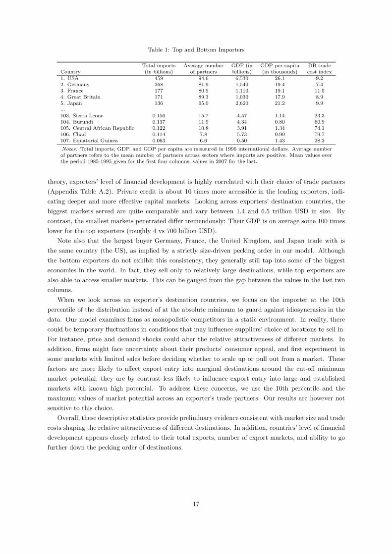
Table 1: Top and Bottom Importers

Total imports Average number GDP (in GDP per capita DB tradeCountry (in billions) of partners billions) (in thousands) cost index1. USA 459 94.6 6,530 26.1 9.22. Germany 268 81.9 1,540 19.4 7.43. France 177 80.9 1,110 19.1 11.54. Great Britain 171 89.3 1,030 17.9 8.95. Japan 136 65.0 2,620 21.2 9.9...103. Sierra Leone 0.156 15.7 4.57 1.14 23.3104. Burundi 0.137 11.9 4.34 0.80 60.9105. Central African Republic 0.122 10.8 3.91 1.34 74.1106. Chad 0.114 7.8 5.73 0.99 79.7107. Equatorial Guinea 0.063 6.6 0.50 1.43 28.3

Notes: Total imports, GDP, and GDP per capita are measured in 1996 international dollars. Average numberof partners refers to the mean number of partners across sectors where imports are positive. Mean values overthe period 1985-1995 given for the first four columns, values in 2007 for the last.

theory, exporters’ level of financial development is highly correlated with their choice of trade partners

(Appendix Table A.2). Private credit is about 10 times more accessible in the leading exporters, indi-

cating deeper and more effective capital markets. Looking across exporters’ destination countries, the

biggest markets served are quite comparable and vary between 1.4 and 6.5 trillion USD in size. By

contrast, the smallest markets penetrated differ tremendously: Their GDP is on average some 100 times

lower for the top exporters (roughly 4 vs 700 billion USD).

Note also that the largest buyer Germany, France, the United Kingdom, and Japan trade with is

the same country (the US), as implied by a strictly size-driven pecking order in our model. Although

the bottom exporters do not exhibit this consistency, they generally still tap into some of the biggest

economies in the world. In fact, they sell only to relatively large destinations, while top exporters are

also able to access smaller markets. This can be gauged from the gap between the values in the last two

columns.

When we look across an exporter’s destination countries, we focus on the importer at the 10th

percentile of the distribution instead of at the absolute minimum to guard against idiosyncrasies in the

data. Our model examines firms as monopolistic competitors in a static environment. In reality, there

could be temporary fluctuations in conditions that may influence suppliers’ choice of locations to sell in.

For instance, price and demand shocks could alter the relative attractiveness of different markets. In

addition, firms might face uncertainty about their products’ consumer appeal, and first experiment in

some markets with limited sales before deciding whether to scale up or pull out from a market. These

factors are more likely to affect export entry into marginal destinations around the cut-off minimum

market potential; they are by contrast less likely to influence export entry into large and established

markets with known high potential. To address these concerns, we use the 10th percentile and the

maximum values of market potential across an exporter’s trade partners. Our results are however not

sensitive to this choice.

Overall, these descriptive statistics provide preliminary evidence consistent with market size and trade

costs shaping the relative attractiveness of different destinations. In addition, countries’ level of financial

development appears closely related to their total exports, number of export markets, and ability to go

further down the pecking order of destinations.

17

Table 2: Top and Bottom Exporters

Average Maximum 10th percentileTotal exports number of Private destination GDP destination GDP

Country (in billions) partners credit (in billions) (in billions)1. USA 351 130.0 0.91 2,690 4.932. Germany 349 141.3 0.93 6,534 4.683. Japan 302 121.0 1.63 6,534 7.504. France 178 139.5 0.86 6,534 4.225. Great Britain 160 146.1 0.95 6,534 4.23...103. Guinea-Bissau 0.025 4.3 0.03 2,544 657104. Central Africa Republic 0.020 3.4 0.07 2,044 477105. Equatorial Guinea 0.015 2.4 0.18 1,362 682106. Rwanda 0.008 3.3 0.09 3,027 719107. Burundi 0.007 3.0 0.09 1,641 524

Notes: Total exports and GDP are measured in 1996 international dollars. Average # of partners refers to themean number of partners across sectors where exports are positive. Private credit is the ratio of the amountof private credit by deposit money banks and other financial institutions to GDP. Mean values over the period1985-1995 given.

5 Results

We next evaluate econometrically the impact of financial development on countries’ choice of trade

partners. We organize the analysis into three steps that correspond to different ways of ranking the

desirability of export destinations. We first consider a pecking order of importers based exclusively

on market size, and ignore cross-country differences in trade costs. We then study the opposite and

complementary case, in which only trade costs matter, while market size plays no role. Finally, we take

an integrated approach and develop summary statistics of market potential that incorporate information

on both size and costs.15

Implicit in our study is that credit conditions affect the level of countries’ exports and their number

of trade partners. For completeness, in Appendix Table A.3 we reproduce results from Manova (2013)

confirming that this is indeed the case.16 Financially advanced economies export relatively more in

sectors more reliant on external capital and in sectors more intensive in intangible assets than in less

financially vulnerable sectors. Countries with stronger financial systems also ship to more destinations in

such industries. These patterns hold in a baseline regression controlling for the exporter’s GDP, country,

year and sector fixed effects, as well as when we condition on the full set of control variables from the

specifications below.

Appendix Figure A.1 provides some canonical examples of the impact of financial development on

trade activity. We consider 6 nations that experienced some of the biggest improvements in financial

conditions in our panel: Bolivia, China, Indonesia, Mexico, Poland, and Thailand. The left-hand side

graphs illustrate how private credit and the aggregate number of export destinations generally moved

closely together within countries over the 1985-1995 period. The right-hand side graphs plot the rise

in the destination count by sector between 1985 and 1995 against sectors’ external finance dependence.

Financial development indeed tended to differentially affect market entry across sectors.17

15In our partial-equilibrium model, the aggregate price index in a destination country also affects its position along thepecking order. In general equilibrium, however, it too would be a function of market size and trade costs.

16Table 5, Panel B, Column 1 in Manova (2013) is identical to Table A.3, Panel A, Column 2 here. The other regressionresults we report are not exactly the same as those in Manova (2013) because of slight differences in the sample and thecontrol variables included.

17These figures are of course only suggestive since many other developments take place in these countries over the1985-1995 period aside from financial development. Our regression analysis will take this into account with a combinationof country, sector and year fixed effects, as well as various controls.

18

5.1 A pecking order of market sizes

We first evaluate how market size influences the pecking order of export destinations and if financial

development affects how far down this pecking order exporting countries reach. We use GDP as our main

measure of market size, since it is the conceptual counterpart to aggregate spending Yi in the model.

For each exporter j, we rank its trade partners in sector s (TPjst) by size, and record the log GDP of

its largest importer, maxi∈TPjst GDPit. We do this separately for each year in the panel to allow for

changes in economic conditions that affect destinations’ attractiveness. Similarly, we note the log GDP

of the destination at the 10th percentile of the distribution, our proxy for mini∈TPjst GDPit for reasons

outlined above. Using these two variables, we estimate specifications (3.1), (3.2), and (3.3).

The results in Panel A of Table 3 lend strong support to our model’s predictions. We find no

systematic variation in the market size of exporters’ largest trade partners across exporters at different

levels of financial development and across sectors at different levels of financial vulnerability (Column

1). By contrast, credit conditions are an important driver of the size of the smallest market that

exporters choose to service (Column 2). Financially advanced economies are able to penetrate smaller

destinations than financially less developed exporters, and this difference is bigger in financially more

vulnerable industries. The coefficients on the two interaction terms of interest (FinDevjt × ExtFinsand FinDevjt × Tangs) are highly statistically significant, both individually and jointly. The last row

in the panel reports the p-value from an F-test of β1 = β2 = 0, and decisively rejects this null hypothesis

at the 0.1% level of confidence.18

These effects are also of sizable economic magnitude. Consider a country such as Mexico that under-

goes financial reforms. Let these reforms increase the amount of private credit available in the economy

(as a share of GDP) by 0.364, which corresponds to one standard deviation in our data. As a result,

Mexico would be able to begin exporting to more destinations by going further down the pecking order

and entering progressively smaller markets. The extent of this expansion into additional export markets

would vary across industries and depend on their reliance on the financial system. Since sectors differ

along two dimensions that are not perfectly correlated with each other (external finance dependence

and asset tangibility), we characterize their differential response with three comparative statics. Take

first two sectors that have the same level of asset tangibility but one requires as much external capital

as the Electrical Machinery industry (ISIC 383, ExtF ins = 0.768), the sector at the 90th percentile

of the distribution, while the other uses as little outside finance as the Leather industry (ISIC 323,

ExtF ins = −0.140), the sector at the 10th percentile. Following financial reforms, the size of Mexico’s

smallest export destination would fall by 16.6 percentage points more in Electrical Machinery than in

Leather. Conversely, two sectors might exhibit the same reliance on external finance but have endow-

ments of tangible assets corresponding to the 10th and 90th percentiles of the distribution, Footwear

(ISIC 324, Tangs = 0.117) and Iron and Steel (ISIC 371, Tangs = 0.458). The size of Mexico’s smallest

trade partner would fall by 10.1 percentage points more in Footwear than in Iron and Steel. Finally,

we account for the actual variation across sectors in the data along both dimensions of financial vulner-

ability, and calculate the total implied impact of financial reforms for each sector. The industry that

experiences the biggest expansion into new export markets would see the size of its smallest destination

fall by 32.0 percentage points more than the industry that benefits the least.

Appendix Table A.4 reports these comparative statics, as well as similar calculations for other mea-

sures of market potential discussed below such as aggregate consumption or bilateral distance. For each

18In unreported results available on request, we have considered a decomposition of GDP into population and GDP percapita, and found consistent results for both components. While the maximum values of log population and log income donot vary systematically across exporters and sectors, the minimum values do much like aggregate GDP.

19

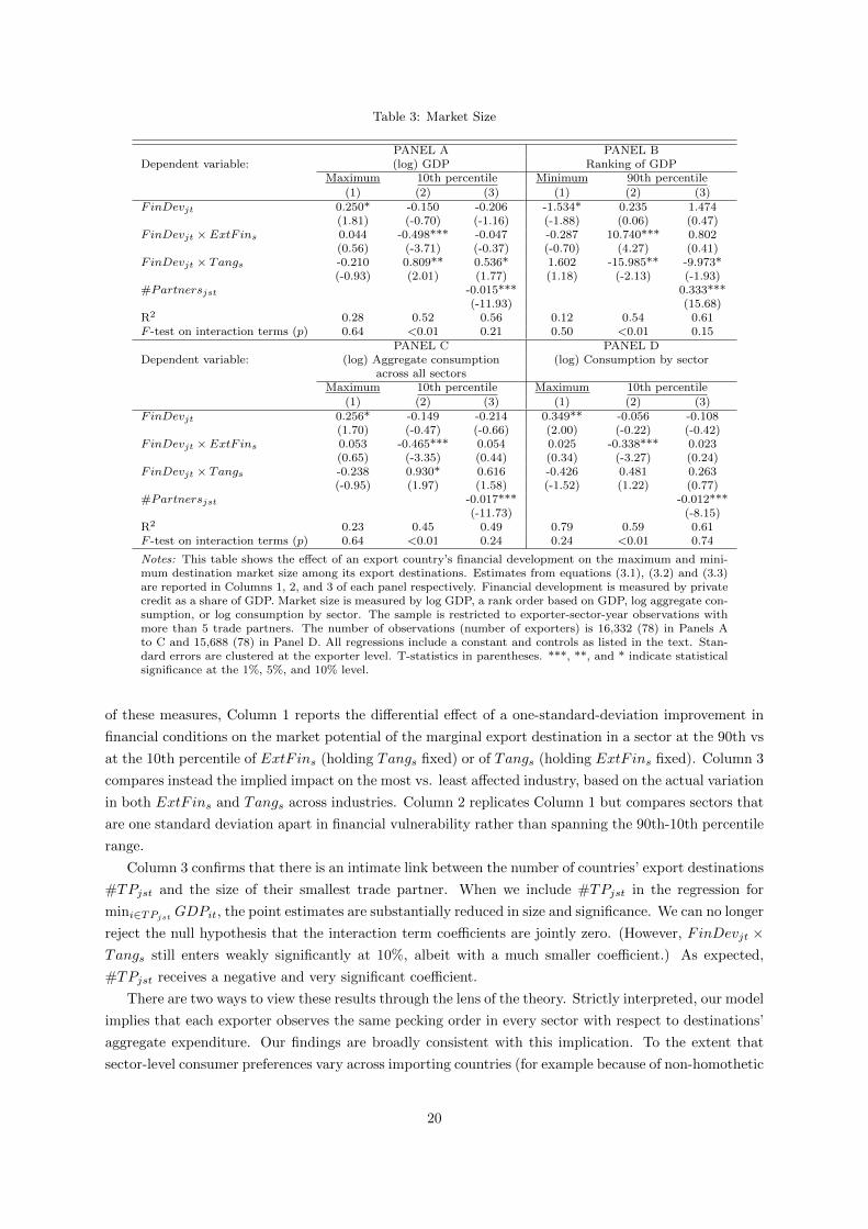
Table 3: Market Size

PANEL A PANEL BDependent variable: (log) GDP Ranking of GDP

Maximum 10th percentile Minimum 90th percentile

(1) (2) (3) (1) (2) (3)FinDevjt 0.250* -0.150 -0.206 -1.534* 0.235 1.474

(1.81) (-0.70) (-1.16) (-1.88) (0.06) (0.47)FinDevjt × ExtF ins 0.044 -0.498*** -0.047 -0.287 10.740*** 0.802

(0.56) (-3.71) (-0.37) (-0.70) (4.27) (0.41)FinDevjt × Tangs -0.210 0.809** 0.536* 1.602 -15.985** -9.973*

(-0.93) (2.01) (1.77) (1.18) (-2.13) (-1.93)#Partnersjst -0.015*** 0.333***

(-11.93) (15.68)R2 0.28 0.52 0.56 0.12 0.54 0.61F -test on interaction terms (p) 0.64 <0.01 0.21 0.50 <0.01 0.15

PANEL C PANEL DDependent variable: (log) Aggregate consumption (log) Consumption by sector

across all sectorsMaximum 10th percentile Maximum 10th percentile

(1) (2) (3) (1) (2) (3)FinDevjt 0.256* -0.149 -0.214 0.349** -0.056 -0.108

(1.70) (-0.47) (-0.66) (2.00) (-0.22) (-0.42)FinDevjt × ExtF ins 0.053 -0.465*** 0.054 0.025 -0.338*** 0.023

(0.65) (-3.35) (0.44) (0.34) (-3.27) (0.24)FinDevjt × Tangs -0.238 0.930* 0.616 -0.426 0.481 0.263

(-0.95) (1.97) (1.58) (-1.52) (1.22) (0.77)#Partnersjst -0.017*** -0.012***

(-11.73) (-8.15)R2 0.23 0.45 0.49 0.79 0.59 0.61F -test on interaction terms (p) 0.64 <0.01 0.24 0.24 <0.01 0.74

Notes: This table shows the effect of an export country’s financial development on the maximum and mini-mum destination market size among its export destinations. Estimates from equations (3.1), (3.2) and (3.3)are reported in Columns 1, 2, and 3 of each panel respectively. Financial development is measured by privatecredit as a share of GDP. Market size is measured by log GDP, a rank order based on GDP, log aggregate con-sumption, or log consumption by sector. The sample is restricted to exporter-sector-year observations withmore than 5 trade partners. The number of observations (number of exporters) is 16,332 (78) in Panels Ato C and 15,688 (78) in Panel D. All regressions include a constant and controls as listed in the text. Stan-dard errors are clustered at the exporter level. T-statistics in parentheses. ***, **, and * indicate statisticalsignificance at the 1%, 5%, and 10% level.

of these measures, Column 1 reports the differential effect of a one-standard-deviation improvement in

financial conditions on the market potential of the marginal export destination in a sector at the 90th vs

at the 10th percentile of ExtF ins (holding Tangs fixed) or of Tangs (holding ExtF ins fixed). Column 3

compares instead the implied impact on the most vs. least affected industry, based on the actual variation

in both ExtF ins and Tangs across industries. Column 2 replicates Column 1 but compares sectors that

are one standard deviation apart in financial vulnerability rather than spanning the 90th-10th percentile

range.

Column 3 confirms that there is an intimate link between the number of countries’ export destinations

#TPjst and the size of their smallest trade partner. When we include #TPjst in the regression for

mini∈TPjst GDPit, the point estimates are substantially reduced in size and significance. We can no longer

reject the null hypothesis that the interaction term coefficients are jointly zero. (However, FinDevjt ×Tangs still enters weakly significantly at 10%, albeit with a much smaller coefficient.) As expected,

#TPjst receives a negative and very significant coefficient.

There are two ways to view these results through the lens of the theory. Strictly interpreted, our model

implies that each exporter observes the same pecking order in every sector with respect to destinations’

aggregate expenditure. Our findings are broadly consistent with this implication. To the extent that

sector-level consumer preferences vary across importing countries (for example because of non-homothetic

20

preferences or home bias), the ranking of destinations might not be exactly the same across sectors. This

could contribute to the residual effect of FinDevjt × Tangs even after controlling for trade partner

intensity in Column 3. Separately, the pecking order is a function of both market size and trade costs

in the model. Since we consider only the former here, potential differences in trade costs across country

pairs and sectors remain unaccounted for.

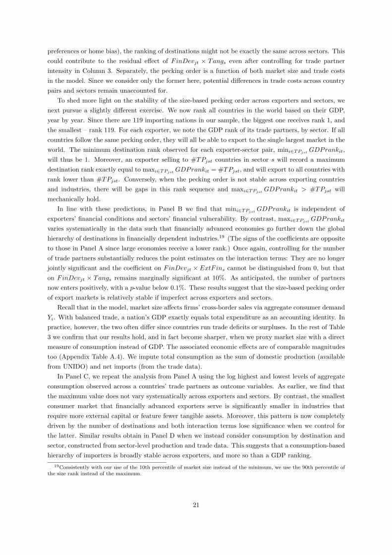
To shed more light on the stability of the size-based pecking order across exporters and sectors, we

next pursue a slightly different exercise. We now rank all countries in the world based on their GDP,

year by year. Since there are 119 importing nations in our sample, the biggest one receives rank 1, and

the smallest – rank 119. For each exporter, we note the GDP rank of its trade partners, by sector. If all

countries follow the same pecking order, they will all be able to export to the single largest market in the

world. The minimum destination rank observed for each exporter-sector pair, mini∈TPjst GDPrankit,

will thus be 1. Moreover, an exporter selling to #TPjst countries in sector s will record a maximum

destination rank exactly equal to maxi∈TPjst GDPrankit = #TPjst, and will export to all countries with

rank lower than #TPjst. Conversely, when the pecking order is not stable across exporting countries

and industries, there will be gaps in this rank sequence and maxi∈TPjst GDPrankit > #TPjst will

mechanically hold.

In line with these predictions, in Panel B we find that mini∈TPjst GDPrankit is independent of

exporters’ financial conditions and sectors’ financial vulnerability. By contrast, maxi∈TPjst GDPrankit

varies systematically in the data such that financially advanced economies go further down the global

hierarchy of destinations in financially dependent industries.19 (The signs of the coefficients are opposite

to those in Panel A since large economies receive a lower rank.) Once again, controlling for the number

of trade partners substantially reduces the point estimates on the interaction terms: They are no longer

jointly significant and the coefficient on FinDevjt × ExtF ins cannot be distinguished from 0, but that

on FinDevjt × Tangs remains marginally significant at 10%. As anticipated, the number of partners

now enters positively, with a p-value below 0.1%. These results suggest that the size-based pecking order

of export markets is relatively stable if imperfect across exporters and sectors.

Recall that in the model, market size affects firms’ cross-border sales via aggregate consumer demand

Yi. With balanced trade, a nation’s GDP exactly equals total expenditure as an accounting identity. In

practice, however, the two often differ since countries run trade deficits or surpluses. In the rest of Table

3 we confirm that our results hold, and in fact become sharper, when we proxy market size with a direct

measure of consumption instead of GDP. The associated economic effects are of comparable magnitudes

too (Appendix Table A.4). We impute total consumption as the sum of domestic production (available

from UNIDO) and net imports (from the trade data).

In Panel C, we repeat the analysis from Panel A using the log highest and lowest levels of aggregate

consumption observed across a countries’ trade partners as outcome variables. As earlier, we find that

the maximum value does not vary systematically across exporters and sectors. By contrast, the smallest

consumer market that financially advanced exporters serve is significantly smaller in industries that

require more external capital or feature fewer tangible assets. Moreover, this pattern is now completely

driven by the number of destinations and both interaction terms lose significance when we control for

the latter. Similar results obtain in Panel D when we instead consider consumption by destination and

sector, constructed from sector-level production and trade data. This suggests that a consumption-based

hierarchy of importers is broadly stable across exporters, and more so than a GDP ranking.

19Consistently with our use of the 10th percentile of market size instead of the minimum, we use the 90th percentile ofthe size rank instead of the maximum.

21

5.2 A pecking order of trade costs

The results in the previous subsection lend strong support to our prediction that financial development

importantly affects countries’ choice of trade partners in terms of market size. We next study the extent

to which this is also true of export costs, the second determinant of the pecking order of destinations in

our model.

Since trade costs are not directly observable, we employ a few standard proxies in the literature. We

first consider bilateral distance Distji, which is arguably associated with the expense of shipping goods

across borders. In this sense it provides an empirical counterpart to the iceberg costs in the model, τij .

To the extent that transportation entails both fixed and variable costs, distance may also partly capture

the fixed cost of exporting, fij . The same would apply if countries that are geographically closer are

more likely to be similar along various economic dimensions that reduce the cost of setting up a trade

partnership. For example, proximate nations might share similar business practices, legal frameworks,

and consumer preferences. Such factors could facilitate the establishment of new commercial links, ease

the maintenance of distribution networks, make researching market potential cheaper, and reduce the

need for customizing products and advertising to local tastes. We therefore do not take a stand as to

whether distance picks up the role of τij or fij in the model. While the measures of market size above

vary by importer and year, distance is a time-invariant characteristic of each exporter-importer pair.

Hence, it is not associated with a uniform pecking order across exporters (e.g. Mexico is closer to US

exporters than Germany, but the converse is true for French exporters).

In Panel A of Table 4, we assess whether financial development allows countries to go further down

the pecking order of export destinations in terms of bilateral distance. According to our model, exporters

will access all markets closer than a maximum distance, but this cut-off will vary across exporters and

sectors. To test this prediction, we record the shortest log distance at which countries export in each year

and industry, mini∈TPjst Distji. As expected, we find that this value does not vary systematically with

credit conditions. Instead, the longest distance at which countries ship their goods, maxi∈TPjst Distji,

rises with FinDevjt×ExtF ins. This implies that stronger financial markets enable firms to fund higher

trade costs, particularly in sectors that demand more external capital. As anticipated, this effect becomes

insignificant when we control for #TPjst, and so it can be attributed to an expansion into more markets:

The expected positive sign on #TPjst indicates that having more export partners is associated with

reaching farther destinations. The insignificant coefficient on FinDevjt × Tangs in Column 2, however,

suggests that financial development does not affect the choice of trade partners differentially across

sectors at different levels of asset tangibility.

We next examine a series of destination-specific proxies for trade costs that reflect the regulatory and

logistical barriers for exporting to country i, Costi. In Panel A of Table 5, we consider the log nominal

cost (per shipping container) required for cross-border sales. The lowest shipping cost observed across

country j’s destinations does not appear to vary systematically with j’s credit conditions (Column 1). By

contrast, the highest shipping cost rises with j’s private credit in sectors with high reliance on external

capital and few collateralizable assets (Column 2). In other words, financially developed exporters are

able to penetrate foreign markets that are more expensive to access. As expected, this pattern can be

explained with the fact that j has more trade partners in such sectors (Column 3).

We find similar results when we instead consider the log number of days it takes for customs trans-

actions to clear (Panel B). On the other hand, the log number of import documents needed does not

appear to generate a pecking order of destinations (Panel C). This suggests that shipping and customs

delays increase exporters’ working capital needs because they force suppliers to stretch their cash flow

22

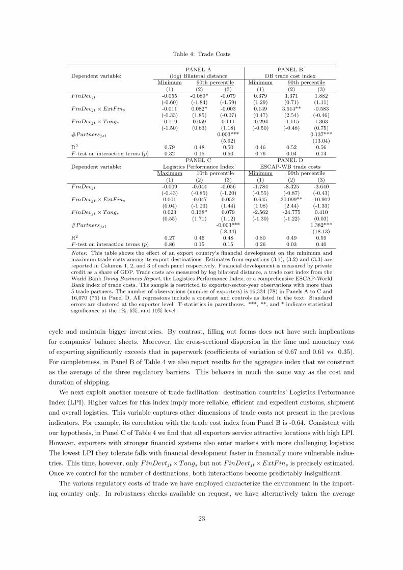
Table 4: Trade Costs

PANEL A PANEL BDependent variable: (log) Bilateral distance DB trade cost index

Minimum 90th percentile Minimum 90th percentile

(1) (2) (3) (1) (2) (3)FinDevjt -0.055 -0.089* -0.079 0.379 1.371 1.882

(-0.60) (-1.84) (-1.59) (1.29) (0.71) (1.11)FinDevjt × ExtF ins -0.011 0.082* -0.003 0.149 3.514** -0.583

(-0.33) (1.85) (-0.07) (0.47) (2.54) (-0.46)FinDevjt × Tangs -0.119 0.059 0.111 -0.294 -1.115 1.363

(-1.50) (0.63) (1.18) (-0.50) (-0.48) (0.75)#Partnersjst 0.003*** 0.137***

(5.92) (13.04)R2 0.79 0.48 0.50 0.46 0.52 0.56F -test on interaction terms (p) 0.32 0.15 0.50 0.76 0.04 0.74

PANEL C PANEL DDependent variable: Logistics Performance Index ESCAP-WB trade costs

Maximum 10th percentile Minimum 90th percentile

(1) (2) (3) (1) (2) (3)FinDevjt -0.009 -0.044 -0.056 -1.784 -8.325 -3.640

(-0.43) (-0.85) (-1.20) (-0.55) (-0.87) (-0.43)FinDevjt × ExtF ins 0.001 -0.047 0.052 0.645 30.099** -10.902

(0.04) (-1.23) (1.44) (1.08) (2.44) (-1.33)FinDevjt × Tangs 0.023 0.138* 0.079 -2.562 -24.775 0.410

(0.55) (1.71) (1.12) (-1.30) (-1.22) (0.03)#Partnersjst -0.003*** 1.382***

(-8.34) (18.13)R2 0.27 0.46 0.48 0.80 0.49 0.59F -test on interaction terms (p) 0.86 0.15 0.15 0.26 0.03 0.40

Notes: This table shows the effect of an export country’s financial development on the minimum andmaximum trade costs among its export destinations. Estimates from equations (3.1), (3.2) and (3.3) arereported in Columns 1, 2, and 3 of each panel respectively. Financial development is measured by privatecredit as a share of GDP. Trade costs are measured by log bilateral distance, a trade cost index from theWorld Bank Doing Business Report, the Logistics Performance Index, or a comprehensive ESCAP-WorldBank index of trade costs. The sample is restricted to exporter-sector-year observations with more than5 trade partners. The number of observations (number of exporters) is 16,334 (78) in Panels A to C and16,070 (75) in Panel D. All regressions include a constant and controls as listed in the text. Standarderrors are clustered at the exporter level. T-statistics in parentheses. ***, **, and * indicate statisticalsignificance at the 1%, 5%, and 10% level.

cycle and maintain bigger inventories. By contrast, filling out forms does not have such implications

for companies’ balance sheets. Moreover, the cross-sectional dispersion in the time and monetary cost

of exporting significantly exceeds that in paperwork (coefficients of variation of 0.67 and 0.61 vs. 0.35).

For completeness, in Panel B of Table 4 we also report results for the aggregate index that we construct

as the average of the three regulatory barriers. This behaves in much the same way as the cost and

duration of shipping.

We next exploit another measure of trade facilitation: destination countries’ Logistics Performance

Index (LPI). Higher values for this index imply more reliable, efficient and expedient customs, shipment

and overall logistics. This variable captures other dimensions of trade costs not present in the previous

indicators. For example, its correlation with the trade cost index from Panel B is -0.64. Consistent with

our hypothesis, in Panel C of Table 4 we find that all exporters service attractive locations with high LPI.

However, exporters with stronger financial systems also enter markets with more challenging logistics:

The lowest LPI they tolerate falls with financial development faster in financially more vulnerable indus-

tries. This time, however, only FinDevtjt×Tangs but not FinDevtjt×ExtFins is precisely estimated.

Once we control for the number of destinations, both interactions become predictably insignificant.

The various regulatory costs of trade we have employed characterize the environment in the import-

ing country only. In robustness checks available on request, we have alternatively taken the average

23

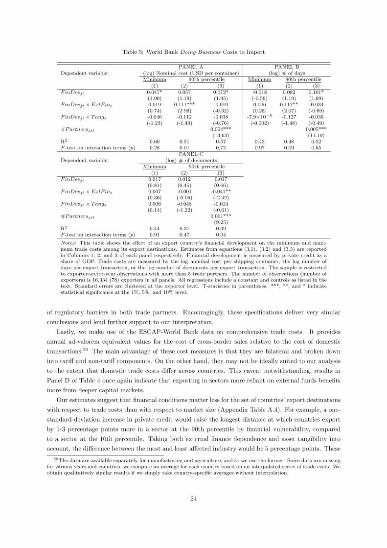
Table 5: World Bank Doing Business Costs to Import

PANEL A PANEL BDependent variable: (log) Nominal cost (USD per container) (log) # of days

Minimum 90th percentile Minimum 90th percentile

(1) (2) (3) (1) (2) (3)FinDevjt 0.047* 0.057 0.072* -0.018 0.082 0.101*

(1.90) (1.19) (1.95) (-0.59) (1.19) (1.69)FinDevjt × ExtF ins 0.019 0.111*** -0.010 0.006 0.117** -0.034

(0.74) (2.96) (-0.32) (0.25) (2.07) (-0.69)FinDevjt × Tangs -0.046 -0.112 -0.038 -7.9×10−5 -0.127 -0.036

(-1.23) (-1.49) (-0.76) (-0.002) (-1.48) (-0.49)#Partnersjst 0.004*** 0.005***

(13.63) (11.19)R2 0.60 0.51 0.57 0.43 0.48 0.52F -test on interaction terms (p) 0.28 0.01 0.72 0.97 0.09 0.65

PANEL CDependent variable: (log) # of documents

Minimum 90th percentile

(1) (2) (3)FinDevjt 0.017 0.012 0.017

(0.81) (0.45) (0.66)FinDevjt × ExtF ins 0.007 -0.001 -0.041**

(0.36) (-0.06) (-2.42)FinDevjt × Tangs 0.006 -0.048 -0.024

(0.14) (-1.22) (-0.61)#Partnersjst 0.001***

(9.25)R2 0.44 0.37 0.39F -test on interaction terms (p) 0.91 0.47 0.04

Notes: This table shows the effect of an export country’s financial development on the minimum and maxi-mum trade costs among its export destinations. Estimates from equations (3.1), (3.2) and (3.3) are reportedin Columns 1, 2, and 3 of each panel respectively. Financial development is measured by private credit as ashare of GDP. Trade costs are measured by the log nominal cost per shipping container, the log number ofdays per export transaction, or the log number of documents per export transaction. The sample is restrictedto exporter-sector-year observations with more than 5 trade partners. The number of observations (number ofexporters) is 16,334 (78) exporters in all panels. All regressions include a constant and controls as listed in thetext. Standard errors are clustered at the exporter level. T-statistics in parentheses. ***, **, and * indicatestatistical significance at the 1%, 5%, and 10% level.

of regulatory barriers in both trade partners. Encouragingly, these specifications deliver very similar

conclusions and lend further support to our interpretation.

Lastly, we make use of the ESCAP-World Bank data on comprehensive trade costs. It provides

annual ad-valorem equivalent values for the cost of cross-border sales relative to the cost of domestic

transactions.20 The main advantage of these cost measures is that they are bilateral and broken down

into tariff and non-tariff components. On the other hand, they may not be ideally suited to our analysis

to the extent that domestic trade costs differ across countries. This caveat notwithstanding, results in

Panel D of Table 4 once again indicate that exporting in sectors more reliant on external funds benefits

more from deeper capital markets.

Our estimates suggest that financial conditions matter less for the set of countries’ export destinations

with respect to trade costs than with respect to market size (Appendix Table A.4). For example, a one-

standard-deviation increase in private credit would raise the longest distance at which countries export

by 1-3 percentage points more in a sector at the 90th percentile by financial vulnerability, compared

to a sector at the 10th percentile. Taking both external finance dependence and asset tangibility into

account, the difference between the most and least affected industry would be 5 percentage points. These

20The data are available separately for manufacturing and agriculture, and so we use the former. Since data are missingfor various years and countries, we compute an average for each country based on an interpolated series of trade costs. Weobtain qualitatively similar results if we simply take country-specific averages without interpolation.

24

economic magnitudes are approximately a sixth of those for GDP.

In summary, it appears that no single measure of trade barriers uniquely characterizes the pecking

order of exporting. Taken collectively, however, the evidence points to financial frictions and trade costs

jointly affecting the location of foreign sales as predicted by theory.

5.3 A pecking order of market potential

Through the lens of our model, the above results suggest that multiple factors govern firms’ choice

of export markets. We next propose that these determinants can be jointly captured with summary

measures of market potential, which indicate the relative desirability of different destinations. In this

section, we develop three such summary measures, and show that financial development affects exporters’

set of trade partners in line with the pecking order implied by these measures.

We first consider a proxy for market potential that combines information about both consumer

demand and trade costs: the log ratio of GDP to distance. This measure is meant to concisely reflect

the basic idea that bigger and more proximate destinations are more attractive. Although it imposes

a specific functional form, we have confirmed that similar results obtain when we adopt alternative

formulations.21 Note that market size is common across all sellers to a given economy, while distance

is country-pair specific. The GDP-to-distance ratio thus allows the relative appeal of an importer to

depend on the identity of the exporter. For example, Canada may be a profitable and proximate market

for the US, but not for other exporters such as Korea, for whom Japan might be preferable.

Using this measure of market potential, we once again record its maximum and minimum (10th

percentile) value across all destinations that exporter j services in sector s. In Panel A of Table 6, we

re-estimate our baseline specifications with these values as outcome variables. We find strong support for

the predictions of the model. As expected, all countries are able to access the markets with the greatest

export potential, but financially advanced economies go further down their hierarchy of destinations in

financially more vulnerable industries. Moreover, both interaction terms are now highly statistically

significant in Column 2, but become insignificant when we control for the number of trade partners in

Column 3. Given the patterns in Panel A of Tables 3 and 4, this suggests that taking both market size

and trade costs into account indeed provides a tighter fit between theory and data. This is not surprising,

since the correlation between GDP and bilateral distance is only 0.06 for the average exporter, and it is

the combination of both country characteristics that determines the pecking order of exporting.

For completeness, in Panel B we perform the same analysis using the log ratio of GDP to the Doing

Business trade cost index as a summary statistic for market potential. In Panel C, we expand this to

the log ratio of GDP to the product of bilateral distance and the trade cost index. We obtain similar

results for these alternative measures as well.

Of note, the implied economic significance of financial development for countries’ choice of trade

partners is considerably larger when we use these summary measures of market potential, than when we

separately consider market size or trade costs (Appendix Table A.4). If a country improves its financial

system by 1 standard deviation, the lowest market potential (=GDP/DB trade costs) among its export

destinations would fall by 22 percentage points more in a financially dependent sector (90th percentile)

relative to a financially less dependent sector (10th percentile). Taking both sectors’ external finance

dependence and asset tangibility into account, the spread between the most and least affected sector

would be 45 percentage points.

21For example, the residuals from regressing (log) importers’ GDP on (log) bilateral distance as the only regressor canbe obtained and used to proxy market potential.

25

Table 6: Market Potential

PANEL A PANEL BDependent variable: (log) GDP/Bilateral distance (log) GDP/DB trade cost index

Maximum 10th percentile Maximum 10th percentile

(1) (2) (3) (1) (2) (3)FinDevjt 0.282* -0.072 -0.150 0.269* -0.305 -0.386*

(1.71) (-0.36) (-1.10) (1.81) (-1.09) (-1.68)FinDevjt × ExtF ins 0.013 -0.540*** 0.091 0.055 -0.677*** -0.032

(0.33) (-3.01) (0.66) (0.62) (-3.72) (-0.20)FinDevjt × Tangs -0.060 0.815* 0.433 -0.220 1.157** 0.767**

(-0.49) (1.89) (1.47) (-0.87) (2.34) (2.13)#Partnersjst -0.021*** -0.022***

(-16.14) (-12.31)R2 0.83 0.60 0.68 0.26 0.53 0.81F -test on interaction terms (p) 0.89 <0.01 0.18 0.69 <0.01 0.11

PANEL C PANEL DDependent variable: (log) GDP/(Bilateral distance × (log) # of exporters by sector

DB trade cost index)Maximum 10th percentile Maximum 10th percentile

(1) (2) (3) (1) (2) (3)FinDevjt 0.310* -0.212 -0.315* 0.032 0.008 -0.012

(1.80) (-0.82) (-1.75) (1.49) (0.09) (-0.15)FinDevjt × ExtF ins 0.013 -0.700*** 0.126 0.008 -0.150** 0.003

(0.27) (-3.11) (0.76) (0.54) (-2.46) (0.06)FinDevjt × Tangs -0.077 1.211** 0.712** -0.051 0.128 0.035

(-0.48) (2.27) (2.07) (-1.61) (0.93) (0.29)#Partnersjst -0.028*** -0.005***

(-16.88) (-10.49)R2 0.81 0.62 0.69 0.87 0.71 0.73F -test on interaction terms (p) 0.89 <0.01 0.07 0.28 0.05 0.96

PANEL E PANEL FDependent variable: (log) Average # of exporters Fixed effect coefficient from

across sectors auxiliary probit regressionMaximum 10th percentile Maximum 10th percentile

(1) (2) (3) (1) (2) (3)FinDevjt 0.035 -0.026 -0.044 0.059 -0.038 -0.059

(1.46) (-0.39) (-0.72) (1.48) (-0.49) (-0.85)FinDevjt × ExtF ins 0.007 -0.191*** -0.045 0.011 -0.201*** -0.033

(0.52) (-4.07) (-1.07) (0.48) (-3.84) (-0.69)FinDevjt × Tangs -0.028 0.218** 0.130* -0.050 0.241** 0.140*

(-0.77) (2.41) (1.94) (-0.79) (2.34) (1.85)#Partnersjst -0.005*** -0.006***

(-12.33) (-12.69)R2 0.17 0.54 0.59 0.88 0.82 0.84F -test on interaction terms (p) 0.74 <0.01 0.12 0.73 <0.01 0.17

Notes: This table shows the effect of an export country’s financial development on the maximum and min-imum market potential among its export destinations. Estimates from equations (3.1), (3.2) and (3.3) arereported in Columns 1, 2, and 3 of each panel respectively. Financial development is measured by privatecredit as a share of GDP. Market potential is measured by the log of GDP / bilateral distance, the log ofGDP / World Bank Doing Business Report trade cost index, the log GDP / (bilateral distance ×World BankDoing Business Report trade cost index), the log number of countries selling to a given destination-sector,the log average number of countries selling to a given destination across sectors, or a destination fixed effectfrom equation (5.1). The sample is restricted to exporter-sector-year observations with more than 5 tradepartners. The number of observations (number of exporters) is 16,332 (78) in Panels A to C and 16,334 (78)in Panels D to F. All regressions include a constant and controls as listed in the text. Standard errors areclustered at the exporter level. T-statistics in parentheses. ***, **, and * indicate statistical significance atthe 1%, 5%, and 10% level.

26

We next take an agnostic approach to what exact factors affect the relative attractiveness of different

foreign markets. To do so, we rely on the principle of revealed preferences: The more popular a given

destination is, the more profitable it must be. We thus count the number of countries exporting to

importer i, #TPist. We obtain this count separately for each sector s since trade conditions (such as

demand and cost structure) could vary not only across destinations, but also across sectors. On the

other hand, by construction #TPist imposes a hierarchy of markets that is shared by all exporters.

This indicator of market potential delivers more evidence in support of our model. In Panel D, we

replace the outcome variable with the log maximum and minimum (10th percentile) values of #TPist

across the countries to which j exports to in sector s. In Panel E, we instead use the log number

of importer i’s trade partners averaged across sectors s. In both cases, we find patterns consistent

with financial development allowing exporters to go further down the pecking order of destinations in

financially vulnerable industries.

Recall from the model that whether bilateral trade occurs depends on both characteristics of the

seller (productivity distribution, wages, trade costs, financial development) and of the buyer (aggregate

demand, trade costs, price index). The number of countries j that sell to i thus reflects how the

combination of exporter and importer factors affect the probability of a trade link between each j and

i. To isolate the contribution of importer-specific determinants without specifying their precise nature,

we finally estimate an auxiliary probit regression with importer fixed effects and examine the relative

magnitude of their coefficients.

Formally, let Tijst be a binary variable equal to 1 if j exports to i in sector s in year t, and zero

otherwise. Assuming a normally distributed error term, the conditional probability of this trade link is:

Pr(Tijst = 1) = Φ(δjt + δit + δst) (5.1)

where Φ is the c.d.f. of the standard normal distribution, and δjt, δit and δst indicate exporter-year,

importer-year and sector-year fixed effects.22 The coefficients δit give a summary measure of the ease and

attractiveness of entering market i in year t. Larger positive coefficients on δit are associated with more

popular destinations. We perform the estimation separately for each year since economic conditions may

vary over time.

Using our estimates of δit in Panel F of Table 6, we record highly statistically and economically

significant results in line with the model’s predictions. We estimate that a one-standard-deviation im-

provement in financial conditions would allow exporters to add 5 more countries down the pecking order

of destinations in an industry highly reliant on external finance (90th percentile) relative to a less de-

pendent industry (10th percentile). Accounting for the variation in both sector measures of financial

vulnerability implies a differential impact of 9 countries between the most and least affected sectors

(Appendix Table A.4).23 Since these fixed effects δit constitute our most agnostic ranking of export

destinations by relative market potential, they are our preferred summary statistic in the remainder of

the empirical analysis.

22We estimate this regression on the full sample of 164 exporting and 175 importing nations in the trade dataset, sinceno control variables are required. This arguably provides the most complete picture of global trade patterns and theirunderlying determinants. Very similar results hold if we instead restrict our attention to the 78 export countries withsufficient data to enter our baseline regressions above.

23Since it is difficult to directly interpret the point estimates in regressions with δit as the measure of market potential,we calculate these comparative statics using the δit-based ranking of countries in Panel D of Table 8 below. This rankingof destinations lends itself to a more natural interpretation.

27

Table 7: Alternative Measures of Financial Development

PANEL A PANEL BFinDevjt measure: Stock market turnover ratio Stock market value traded-to-GDP

Maximum 10th percentile Maximum 10th percentile

(1) (2) (3) (1) (2) (3)FinDevjt -0.004 -0.041* -0.018 -0.0003 -0.030 0.011

(-0.32) (-1.78) (-0.76) (-0.02) (-0.59) (0.28)FinDevjt × ExtF ins -0.021** -0.125*** -0.027 -0.010 -0.094* 0.017

(-2.31) (-5.36) (-1.23) (-0.92) (-1.88) (0.40)FinDevjt × Tangs 0.034 0.182** 0.054 -0.010 0.206* 0.010

(0.81) (2.65) (0.78) (-0.25) (1.70) (0.10)#Partnersjst -0.005*** -0.005***

(-13.08) (-13.31)R2 0.92 0.85 0.87 0.92 0.85 0.87F -test on interaction terms (p) 0.08 <0.01 0.34 0.50 0.12 0.86

PANEL C PANEL DFinDevj measure: Risk of contract repudiation Risk of expropriation

Maximum 10th percentile Maximum 10th percentile

(1) (2) (3) (1) (2) (3)FinDevj × ExtF ins -0.002 -0.065*** -0.010 -0.005 -0.052*** 0.011

(-0.19) (-3.91) (-0.73) (-0.58) (-2.82) (0.71)FinDevj × Tangs -0.033 0.078* 0.016 -0.001 0.111** 0.055

(-0.95) (1.74) (0.47) (-0.03) (2.03) (1.23)#Partnersjst -0.006*** -0.006***

(-12.74) (-12.78)R2 0.92 0.84 0.87 0.92 0.84 0.87F -test on interaction terms (p) 0.37 <0.01 0.70 0.70 0.02 0.30

PANEL E PANEL FFinDevjt measure: Accounting standards Private credit (extended controls)

Maximum 10th percentile Maximum 10th percentile

(1) (2) (3) (1) (2) (3)FinDevjt 0.029 -0.069 -0.073

(1.37) (-0.84) (-1.05)FinDevjt × ExtF ins -0.106* -0.393** -0.039 0.019 -0.170** -0.032

(-1.73) (-2.13) (-0.25) (0.66) (-2.62) (-0.61)FinDevjt × Tangs 0.026 0.517 0.150 -0.072 0.322** 0.180**

(0.11) (1.52) (0.40) (-1.11) (2.52) (2.16)#Partnersjst -0.006*** -0.006***

(-11.66) (-12.71)R2 0.97 0.88 0.91 0.92 0.85 0.87F -test on interaction terms (p) 0.22 0.09 0.90 0.50 0.01 0.10

Notes: This table shows that the effect of export countries’ financial development on their choice of exportdestinations is robust to alternative measures of financial development. Estimates from equations (3.1), (3.2)and (3.3) are reported in Columns 1, 2, and 3 of each panel respectively. Financial development is measuredby the stock market turnover ratio, stock market value traded as a share of GDP, the risk of contract repu-diation, the risk of expropriation, or accounting standards. Market potential is measured by a destinationfixed effect from equation (5.1). The sample is restricted to exporter-sector-year observations with more than5 trade partners. The number of observations (number of exporters) from Panels A to F are: 12,687 (55),13,224 (56), 12,091 (42), 12,091 (42), 9,962 (34), and 11,821 (42). All regressions include a constant and con-trols as listed in the text. Standard errors are clustered at the exporter level. T-statistics in parentheses.***, **, and * indicate statistical significance at the 1%, 5%, and 10% level.

28

Table 8: Specification Checks

PANEL A PANEL BDependent variable: Fixed effect coefficient from Fixed effect coefficient from

auxiliary probit regression auxiliary probit regressionFinV uls measure: External finance dependence Asset tangibility

Maximum 10th percentile Maximum 10th percentile

(1) (2) (3) (1) (2) (3)FinDevjt 0.044 0.037 -0.016 0.062 -0.094 -0.068

(1.26) (0.52) (-0.26) (1.51) (-1.24) (-1.00)FinDevjt × FinV uls 0.011 -0.204*** -0.034 -0.051 0.258** 0.142*

(0.50) (-3.86) (-0.72) (-0.79) (2.46) (1.87)#Partnersjst -0.006*** -0.006***

(-12.68) (-13.08)R2 0.88 0.82 0.84 0.88 0.82 0.84

PANEL C PANEL DDependent variable: Fixed effect coefficient from Ranking of fixed effect coefficient

auxiliary probit regression from auxiliary probit regression90th percentile Minimum Minimum 90th percentile

(1) (2) (3) (1) (2) (3)FinDevjt 0.117** 0.143 0.102 -1.126 2.620 4.216

(2.04) (1.19) (1.07) (-1.58) (0.48) (0.85)FinDevjt × ExtF ins -0.085* -0.354*** -0.025 -0.283 14.958*** 2.182

(-1.67) (-5.27) (-0.36) (-0.75) (3.87) (0.62)FinDevjt × Tangs 0.010 0.356** 0.157 0.770 -19.607** -11.878*

(0.09) (2.41) (1.45) (0.63) (-2.36) (-1.95)#Partnersjst -0.011*** 0.428***

(-15.93) (12.44)R2 0.84 0.76 0.80 0.09 0.54 0.59F -test on interaction terms (p) 0.19 <0.01 0.35 0.71 <0.01 0.15

PANEL E PANEL FDependent variable: Fixed effect coefficient from Fixed effect coefficient from

auxiliary logit regression auxiliary LPM regressionMaximum 10th percentile Maximum 10th percentile

(1) (2) (3) (1) (2) (3)FinDevjt 0.085 -0.054 -0.092 0.014 -0.012 -0.016

(1.21) (-0.40) (-0.74) (1.48) (-0.71) (-1.03)FinDevjt × ExtF ins 0.020 -0.369*** -0.066 0.002 -0.045*** -0.012

(0.50) (-3.81) (-0.75) (0.45) (-4.25) (-1.22)FinDevjt × Tangs -0.081 0.466** 0.282** -0.012 0.048** 0.028*

(-0.69) (2.43) (2.02) (-0.81) (2.19) (1.72)#Partnersjst -0.010*** -0.001***

(-2.41) (-12.59)R2 0.84 0.79 0.81 0.92 0.88 0.89F -test on interaction terms (p) 0.78 <0.01 0.12 0.72 <0.01 0.15

PANEL G PANEL HDependent variable: Fixed effect coefficient from Fixed effect coefficient from auxiliary

auxiliary probit regression (pooled) probit regression (by sector-year)Maximum 10th percentile Maximum 10th percentile

(1) (2) (3) (1) (2) (3)FinDevjt 0.068* -0.066 -0.086 0.039 -0.016 -0.042

(1.79) (-0.95) (-1.32) (0.95) (-0.17) (-0.49)FinDevjt × ExtF ins 0.009 -0.185*** -0.031 0.046 -0.280*** -0.075

(0.40) (-3.86) (-0.70) (1.41) (-4.51) (-1.45)FinDevjt × Tangs -0.047 0.224** 0.131* -0.086 0.265** 0.140

(-0.74) (2.32) (1.80) (-1.49) (2.11) (1.34)#Partnersjst -0.005*** -0.007***

(-11.79) (-13.78)R2 0.15 0.52 0.57 0.90 0.76 0.79F -test on interaction terms (p) 0.76 <0.01 0.18 0.25 <0.01 0.14

Notes: This table shows that the effect of export countries’ financial development on their choice of export desti-nations is robust to alternative estimation methods. Estimates from equations (3.1), (3.2) and (3.3) are reportedin Columns 1, 2, and 3 of each panel respectively. Financial development is measured by private credit as a shareof GDP. Market potential is measured by a destination fixed effect from equation (5.1). The sample is restrictedto exporter-sector-year observations with more than 5 trade partners. The number of observations (number of ex-porters) is 16,334 (78) in all panels. All regressions include a constant and controls as listed in the text. Standarderrors are clustered at the exporter level. T-statistics in parentheses. ***, **, and * indicate statistical significanceat the 1%, 5%, and 10% level.

29

5.4 Robustness

We conclude by showing that our empirical findings survive a series of specification checks that

reinforce our conclusions. We report these robustness tests using the fixed effects from the auxiliary

probit regression, but qualitatively similar patterns hold for the other measures we have employed as

well.

Our analysis has relied on the amount of private credit in an economy as a signal of financial market

development. In Table 7, we first confirm that other indicators of financial sector activity (also from

Beck et al. 2000) deliver comparable findings. In Panel A, we consider the stock market turnover

ratio, constructed as the value of total shares traded divided by stock market capitalization. While

private credit reflects firms’ use of debt financing, value traded captures the availability and liquidity of

equity capital. In Column 2, we find that active stock markets help exporters in reaching less attractive

destinations, and this is especially true in financially vulnerable sectors. (Although there is a statistically

significant effect present for the largest market as well in Column 1, it is much weaker in comparison.)

Similar patterns emerge in Panel B, where we study stock market value traded as a share of GDP. This

suggests that loan access and stock issuance are both relevant to trade activity, presumably because they

provide alternative sources of funding.24

Private credit and stock market activity are outcome-based measures that reflect the actual availabil-

ity and use of financial capital in a country. The health of the financial system in turn depends on the

underlying institutions that support financial contracts. For this reason, the prior literature has exploited

different institutional measures to gauge the variation in financial development across nations. As Panels

C, D, and E demonstrate, our results are qualitatively the same when we follow this strategy: Using the

risk of contract repudiation, the risk of expropriation, or accounting standards instead of private credit

delivers similar patterns for exporters’ choice of trade partners.25

We further verify that our measure of financial development does not simply pick up the strength of

the broader institutional environment. To do so, we expand the set of control variables to include the

interactions of rule of law and corruption with each of the two sector indicators of financial vulnerability.26

Panel F shows that this does not affect the coefficients of interest.

We next ensure that our findings are not driven by specific functional form assumptions. In Panels

A and B of Table 8, we include only one interaction term at a time. The magnitude and statistical

significance of the point estimates are barely affected, consistent with the low correlation between the

two sector measures. This supports the idea that ExtF ins and Tangs reflect separate dimensions of

financial vulnerability that are both important in practice.

In the rest of Table 8, we consider a series of other perturbations to the baseline functional form that

leave our results unchanged or stronger. In Panel C, we set the outcome variables equal to the 90th

percentile and the minimum value of market potential across a country’s export destinations, instead of

24In unreported results available on request, we have found that the size of the stock market itself (measured by stockmarket capitalization divided by GDP) does not affect exporters’ trade partners systematically. This is consistent withprior evidence in the literature that stock market activity can sometimes be a more informative measure of financial sectordevelopment than stock market size (c.f. Manova 2008). We have also studied total liquid liabilities (the sum of currencyin circulation, demand- and interest-bearing liabilities of all banks and non-bank financial intermediaries), divided by GDP.This ratio provides an alternative index of financial depth and of the overall size of the financial intermediary sector. Theresults are in line with our other findings, though the coefficients are less precisely estimated.

25The indices for the risk of contract repudiation or expropriation range from 0 to 10, while the rating of accountingstandards varies in the unit interval. All three measures come from La Porta et al. (1998), and are available for a smallersample of 34-42 export countries. Since they are time-invariant, the main effect of financial development in these regressionsis subsumed by the exporter country fixed effects.

26These two measures also come from La Porta et al. (1998), do not vary over time, and are available for 42 of theexport countries in the sample.

30

−.6

−.4

−.2

0.2

Coe

ffici

ent o

n F

inD

ev x

Ext

Fin

020406080100Distribution of Market Potential (Percentile)

(a)

−.2

0.2

.4.6

Coe

ffici

ent o

n F

inD

ev x

Tan

g

020406080100Distribution of Market Potential (Percentile)

(b)

Fig. 6: This figure shows the effect of an export country’s financial development on market potential at the 100th, 95th,90th, ..., 10th, 5th, and 0th percentile of the distribution of market potential among its export destinations. Plots (a) and(b) present coefficient estimates for FinDevjt × ExtF ins and FinDevjt × Tangs, respectively, from estimating equation(3.1) for each of these 21 percentiles as the outcome variable. The dashed lines correspond to the 95% confidence intervalaround these coefficient estimates. Financial development is measured by private credit as a share of GDP. Market potentialis measured by a destination fixed effect from equation (5.1). Coefficients at the 100th percentile (maximum) correspondto coefficients in Table 6 Panel F Column 1, and at the 10th percentile to Column 2.

the maximum and the 10th percentile as we have done so far. In Panel D, we study importers’ rank

based on their fixed effects from the auxiliary probit regression, instead of the value of those fixed effects.

In Panels E and F, we estimate the first-stage equation (5.1) either with logit or with a linear probability

model, instead of with probit. In Panel G, we run the first-stage probit in the pooled panel for 1985-1995

with year dummies, instead of year-by-year. This imposes time-invariant importer fixed effects, such

that the hierarchy of destinations is stable over this period. Conversely, in Panel H we allow the pecking

order to vary flexibly both across time and across sectors, by estimating the first stage separately for

each sector-year pair.

We next conduct a more stringent test of our model’s predictions. If countries follow a strict pecking

order of exporting, we should observe nestedness: no country should enter the Nth most popular market

unless it also serves the (N-1)th most popular market. We have so far provided indirect evidence for

nestedness by finding significant coefficients in equation (3.2) but not in (3.1) and (3.3). In particular,

these results imply a one-to-one mapping between an exporter’s number of destinations and the minimum

market potential among them, such that all destinations with higher market potential must also be served

with no gaps in the pecking order. As a more direct test of nestedness, we now estimate specification

(3.1) for 21 values from the distribution of market potential across an exporter’s trade partners: 100th

percentile (=maximum), 95th percentile, 90th percentile, ... , 10th percentile, 5th percentile, and 0th

percentile (=minimum). For each of these 21 regressions, we record the coefficients on the two interactions

of interest, and plot them against the percentile corresponding to the outcome variable.27

Figure 6 displays patterns strongly indicative of nestedness. With perfect nestedness, financial devel-

opment should not affect the maximum market potential among a country’s destinations differentially

across sectors with different levels of financial vulnerability. As we have already seen, the estimated

coefficients are indeed 0 for both sector measures when the outcome is the 100th percentile of market

potential. As we move right along the horizontal axis from the 100th to the 0th percentile, the line

27Bustos et al. (2012) employ other econometric tests of nestedness that are not readily applicable to difference-in-differences estimation. We leave the application of their methodology to the study of export-market nestedness withfinancial frictions to future work.

31

generally slopes down for external finance dependence and generally slopes up for asset tangibility. In

other words, financial development allows countries to smoothly go further down their pecking order of

destinations in financially more vulnerable sectors, relative to financially less vulnerable sectors. More-

over, any non-monotonicities in the precise point estimates disappear when we take into account the

95-percent confidence interval around these estimates.

Figure 6 indicates that the effects of financial development become statistically significant around and

below the 70th percentile of the distribution of export destinations by market potential. How important

are these destinations to countries’ aggregate exports? Our difference-in-differences identification strat-

egy prevents us from calculating implied magnitudes for effects at the country level. Summary statistics

nevertheless suggest that although the distribution of trade flows across destinations is very skewed, the

contribution of destinations outside the top deciles is not trivial. Appendix Figure A.2 plots the share of

exports (summed across sectors) going to each of ten deciles of destinations grouped by market potential,

averaged across exporting countries in 1995. The top, second and third deciles capture respectively about

65%, 18% and 7% of the average country’s exports. Very similar patterns obtain whether we rank all

potential destinations based on our preferred measure of market potential or order actual destinations

served separately for each exporter. Expansion into new markets abroad can also add substantially to

export growth within countries over time. We identify the new destinations that each exporter in our

data entered between 1985 and 1995. For the average country, sales to new markets contribute 10.9%

to total exports in 1995 (standard deviation 16.7%) and 14.5% to total export growth between 1985 and

1995 (standard deviation 80.3%).

Finally, we have performed sensitivity checks to address potential concerns with reporting errors in

trade values (available on request). While classical measurement error would introduce noise and bias our

results downwards, a particular form of non-classical measurement error might bias our results upwards:

If very low trade flows are systematically under-reported, the pecking order of countries would not be

affected, but the coefficients in regressions for the minimum market potential might be overestimated.

This might arise for two reasons. First, the raw data report only positive bilateral trade flows, in

thousands of dollars. Hence the lowest observed value is $1,000, and any unobserved exporter-importer-

sector triplet is assumed to conduct zero trade. Our results, however, remain robust when we set to 0

all observed positive trade flows below the 1st percentile ($5,000) or below $100,000.

Second, less developed nations may be more likely to misreport trade flows. Note that all of our

specifications already control for the exporter’s level of overall development (GDP per capita), and

Panel F of Table 7 shows that our findings also hold conditioning on the exporter’s corruption level. We

have additionally checked that our results survive when, in the first-stage auxiliary probit regression,

we drop origin and destination countries with GDP per capita below the 5th percentile, or exporter-

importer-sector triplets with annual export growth above 100% that might signal misreporting. We have

also estimated a weighted first-stage probit regression, where we weighted observations by the exporter’s

GDP per capita or anti-corruption index.

The stability of the results across these robustness checks bolsters our conclusion that countries’ level

of financial development is an important determinant of their export behavior, and the range of markets

they choose to service in particular.

32

6 Conclusion

This paper establishes that exporters follow a pecking order of destinations, but financial frictions

disrupt their decision to enter foreign markets. We develop a theoretical model to illustrate how firms

add destinations in decreasing order of profitability, determined by market size and trade costs. Credit

constraints limit firms’ access to financial resources and prevent them from entering all markets they could

serve in the first best. This distortion is alleviated in exporting countries with better-functioning capital

markets. As a result, financially advanced economies export to more destinations by going further down

the pecking order. This effect is especially pronounced in financially vulnerable sectors characterized by

high external finance dependence and low asset tangibility.

We confirm these theoretical predictions empirically by estimating model-consistent relationships

between characteristics of exporters’ destination countries and credit conditions at home. Using aggregate

bilateral trade data, we analyze how the maximum and minimum values of market potential amongst an

exporter’s trade partners vary with exporters’ financial development and sectors’ financial vulnerability.

In the process, we develop a model-consistent hierarchy of destinations based on observed market size

and trade costs, as well as on unobserved market potential inferred from actual trade links. Our findings

are robust to a series of specification checks and variable measurement.

Our results imply that financial institutions importantly affect the number and identity of countries’

trade partners. This adds to prior evidence in the literature that international trade linkages have a wide

range of economic repercussions that crucially depend on countries’ characteristics, such as overall level

of development and role in global goods and capital markets. A promising direction for future work lies

at the intersection of these two lines of research. By improving domestic financial conditions, countries

can expand their set of export destinations and foster entry into new locations. A key question for

policy makers in developing economies is how this would shape economic growth, volatility, cross-border

productivity spillovers, and the transmission of shocks across nations.

References

Amiti, M. and D. E. Weinstein (2011). Exports and financial shocks. Quarterly Journal of Eco-nomics 126 (4), 1841–1877.

Armenter, R. and M. Koren (2014). A balls-and-bins model of trade. American Economic Review 104 (7),2127–2151.

Arvis, J.-F., Y. Duval, B. Shepherd, and C. Utoktham (2013). Trade costs in the developing world: 1995- 2010. World Bank Policy Research Working Paper No. 6309 .

Baxter, M. and M. A. Kouparitsas (2005). Determinants of business cycle comovement: a robust analysis.Journal of Monetary Economics 52, 113–157.

Beck, T., A. Demirguc-Kunt, and R. Levine (2000). A new database on the structure and developmentof the financial sector. World Bank Economic Review 14 (3), 597–605.

Berman, N. and J. Hericourt (2010). Financial factors and the margins of trade: Evidence from cross-country firm-level data. Journal of Development Economics 93 (2), 206–217.

Bernard, A. B., J. B. Jensen, S. J. Redding, and P. K. Schott (2007). Firms in international trade.Journal of Economic Perspectives 21 (3), 105–130.

Bernard, A. B., S. J. Redding, and P. K. Schott (2011). Multiproduct firms and trade liberalization.Quarterly Journal of Economics 126 (3), 1271–1318.

33

Braun, M. (2003). Financial contractibtility and asset hardness. University of California- Los Angelesmimeo.

Bricongne, J.-C., L. Fontagne, G. Gaulier, D. Taglioni, and V. Vicard (2012). Firms and the globalcrisis: French exports in the turmoil. Journal of International Economics 87 (1), 134–146.

Burstein, A., C. Kurz, and L. Tesar (2008). Trade, production sharing, and the international transmissionof business cycles. Journal of Monetary Economics 55, 775–795.

Bustos, S., C. Gomez, R. Hausmann, and C. A. Hidalgo (2012). The dynamics of nestedness predictsthe evolution of industrial ecosystems. PLoS One 7 (11), e49393.

Caselli, F. (2005). Accounting for cross-country income differences. In P. Aghion and S. Durlauf (Eds.),Handbook of Economic Growth, pp. 679–741. Elsevier.

Chor, D. and K. Manova (2012). Off the cliff and back? Credit conditions and international trade duringthe global financial crisis. Journal of International Economics 87, 117–133.

Clark, T. E. and E. van Wincoop (2001). Borders and business cycles. Journal of International Eco-nomics 55, 59–85.

de Loecker, J. (2007). Do exports generate higher productivity? Evidence from Slovenia. Journal ofInternational Economics 73 (1), 69–98.

Dhingra, S. (2013). Trading away wide brands for cheap brands. American Economic Review 103 (6),2554–2584.

Eaton, J. and S. Kortum (2002). Technology, geography, and trade. Econometrica 70 (5), 1741–1779.

Eaton, J., S. Kortum, and F. Kramarz (2011a). An anatomy of international trade: Evidence fromFrench firms. Econometrica 79 (5), 1453–1498.

Eaton, J., S. Kortum, B. Neiman, and J. Romalis (2011b). Trade and the global recession. NBERWorking Paper No. 16666 .

Feenstra, R. C. (2000). World trade flows, 1980-1997. Center for International Data, University ofCalifornia Davis.

Feenstra, R. C., Z. Li, and M. Yu (forthcoming). Exports and credit constraints under incompleteinformation: Theory and evidence from China. Review of Economics and Statistics.

Foley, F. C. and K. Manova (forthcoming). International trade, multinational activity, and corporatefinance. Annual Review of Economics.

Frankel, J. A. and A. K. Rose (1998). The endogeneity of the optimum currency area criteria. TheEconomic Journal 108 (449), 1009–1025.

Goldberg, P. K., A. K. Khandelwal, N. Pavcnik, and P. Topalova (2010). Imported intermediate inputsand domestic product growth: Evidence from India. Quarterly Journal of Economics 125 (4), 1727–1767.

Haveman, J. Jon Haveman’s industry concordances. http://www.macalester.edu/research/

economics/PAGE/HAVEMAN/Trade.Resources/tradeconcordances.html. Accessed: 05/09/2014.

Helpman, E., M. J. Melitz, and Y. Rubinstein (2008). Estimating trade flows: Trading partners andtrading volumes. Quarterly Journal of Economics 123 (2), 441–487.

Kali, R., F. Mendez, and J. Reyes (2007). Trade structure and economic growth. The Journal ofInternational Trade and Economic Development 16 (2), 245–269.

La Porta, R., F. Lopez-de Silanes, A. Shleifer, and R. W. Vishny (1998). Law and finance. Journal ofPolitical Economy 106 (6), 1113–1155.

34

Manova, K. (2008). Credit constraints, equity market liberalizations and international trade. Journal ofInternational Economics 76, 33–47.

Manova, K. (2013). Credit constraints, heterogeneous firms, and international trade. Review of EconomicStudies 80, 711–744.

Manova, K., S.-J. Wei, and Z. Zhang (forthcoming). Firm exports and multinational activity undercredit constraints. Review of Economics and Statistics.

Manova, K. and Z. Zhang (2012). Export prices across firms and destinations. Quarterly Journal ofEconomics 127 (1), 379–436.

Mayer, T., M. J. Melitz, and G. I. P. Ottaviano (2014). Market size, competition, and the product mixof exporters. American Economic Review 104 (2), 495–536.

Melitz, M. J. (2003). The impact of trade on intra-industry reallocations and aggregate industry pro-ductivity. Econometrica 71 (6), 1695–1725.

Melitz, M. J. and G. I. P. Ottaviano (2008). Market size, trade, and productivity. Review of EconomicStudies 75, 295–316.

Minetti, R. and S. C. Zhu (2011). Credit constraints and firm export: Microeconomic evidence fromItaly. Journal of International Economics 83 (2), 109–125.

Muuls, M. (2008). Exporters and credit constraints: a firm-level approach. London School of Economicsmimeo.

Novy, D. (2013). Gravity redux: measuring international trade costs with panel data. Economic In-quiry 51 (1), 101–121.

Rodrik, D. (2005). Growth strategies. In P. Aghion and S. Durlauf (Eds.), Handbook of EconomicGrowth, pp. 967–1014. Elsevier.

Verhoogen, E. (2008). Trade, quality upgrading, and wage inequality in the Mexican manufacturingsector. Quarterly Journal of Economics 123 (2), 489–530.

35

Appendix

Table A.1: Export Destinations, Growth, and Volatility

Dependent variable: ∆(Exports) σ(∆(Exports)) ∆(Exports) ∆(GDPpc) σ(∆(GDPpc)) ∆(GDPpc)(1) (2) (3) (4) (5) (6)

(log) # of export destinations1985 5.985** -0.149** 11.851*** 1.231* -0.019* 2.113**(2.60) (-2.34) (6.21) (1.74) (-1.72) (2.45)

(log) total exports1985 -0.747 -0.010 -1.208*** 0.027 -0.001 -0.042(-1.15) (-0.53) (-2.67) (0.13) (-0.33) (-0.22)

∆(# of export destinations) 1.772*** 0.266*(6.34) (1.81)

R2 0.19 0.29 0.44 0.17 0.24 0.21

Notes: ∆(x) and σ(∆(x)) refer to the mean and standard deviation of the growth rate of x between 1986-1995. N = 90 ex-porters in all regressions. All regressions include a constant term. Heteroskedastic robust standard errors used. T-statistics inparentheses. ***, **, and * indicate statistical significance at the 1%, 5%, and 10% level.

Table A.2: Correlations for Variables in Tables 1 and 2

PANEL A- ImportersVariable 1 2 3 4 51. Total imports —2. Average # of partners 0.79 —3. GDP 0.86 0.60 —4. GDP per capita 0.63 0.80 0.40 —5. Trade cost index -0.34 -0.61 -0.22 -0.63 —PANEL B- ExportersVariable 1 2 3 4 51. Total exports —2. Average # of partners 0.77 —3. Private credit 0.63 0.78 —4. Max. of export partners’ GDP 0.24 0.61 0.49 —5. 10th percentile of distr. of -0.29 -0.56 -0.47 -0.63 —

export partners’ GDP

Notes: 104 countries in Panel A, 107 in Panel B.

Table A.3: Financial Development and Trade Activity

PANEL A PANEL BAt least 1 partner More than 5 partners

Dependent variable: (log) Exports # TP (log) Exports # TP

(1) (2) (1) (2)FinDevjt 0.150 -2.227 0.229 -3.732

(0.57) (-0.46) (0.70) (-0.58)FinDevjt × ExtF ins 1.564*** 41.942*** 1.356*** 29.872***

(8.31) (13.44) (4.38) (5.08)FinDevjt × Tangs -1.171* -17.045** -1.680** -18.074

(-1.89) (-2.12) (-2.06) (-1.53)Controls log(GDPjt) and log(GDPjt), K/L,H/L,N/L,

j, s, t fixed effects log(GDPPCjt), interactionsand j, s, t fixed effects

R2 0.82 0.90 0.80 0.88

Notes: # TP refers to the number of trade partners of the exporter in each sector.The measure of financial development is private credit. The unit of observation is atthe exporter-sector-year level. The sample is restricted to observations with at least1 trade partner in Panel A and more than 5 trade partners in B. The number of ob-servations (number of exporters) is 26,900 (107) in Panel A and 16,334 (78) in PanelB. Panel B controls are the same as those listed in the text. Standard errors areclustered at the exporter level. T-statistics in parentheses. ***, **, and * indicatestatistical significance at the 1%, 5%, and 10% level.

36

0.1

.2.3

.4.5

Priv

ate

Cre

dit

2030

4050

60#

of e

xpor

t des

tinat

ions

1985 1990 1995

# export dest.Private credit

Bolivia

(a)

−10

010

2030

Cha

nge

in #

of

expo

rt d

estin

atio

ns

−.5 0 .5 1External Finance Dependence

Bolivia

(b)

.7.7

5.8

.85

Priv

ate

Cre

dit

8010

012

014

016

0#

of e

xpor

t des

tinat

ions

1985 1990 1995

# export dest.Private credit

China

(c)

050

100

150

Cha

nge

in #

of

expo

rt d

estin

atio

ns

−.5 0 .5 1External Finance Dependence

China

(d)

.1.2

.3.4

.5

Priv

ate

Cre

dit

100

110

120

130

140

# of

exp

ort d

estin

atio

ns

1985 1990 1995

# export dest.Private credit

Indonesia

(e)

020

4060

80

Cha

nge

in #

of

expo

rt d

estin

atio

ns

−.5 0 .5 1External Finance Dependence

Indonesia

(f)

Fig. A.1: For each country (Bolivia, China, and Indonesia), we plot the number of export destinations and financialdevelopment (private credit) from 1985 to 1995 (left side), and the change in the number of export destinations from 1985to 1995 by industry against industries’ external finance dependence (right side).

37

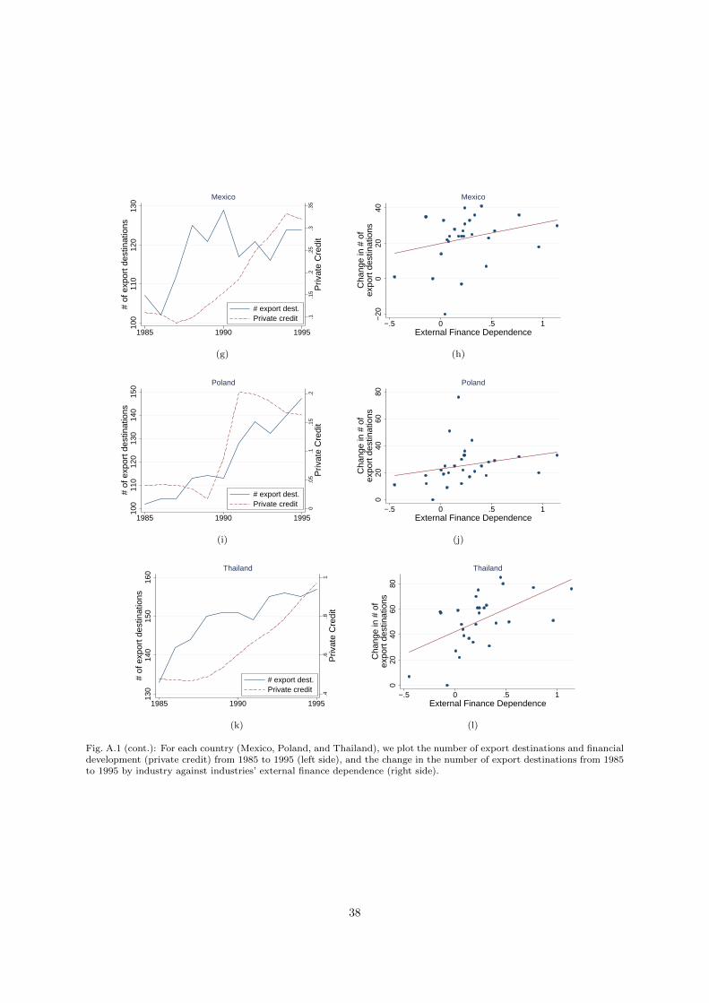
.1.1

5.2

.25

.3.3

5

Priv

ate

Cre

dit

100

110

120

130

# of

exp

ort d

estin

atio

ns

1985 1990 1995

# export dest.Private credit

Mexico

(g)

−20

020

40

Cha

nge

in #

of

expo

rt d

estin

atio

ns

−.5 0 .5 1External Finance Dependence

Mexico

(h)

0.0

5.1

.15

.2

Priv

ate

Cre

dit

100

110

120

130

140

150

# of

exp

ort d

estin

atio

ns

1985 1990 1995

# export dest.Private credit

Poland

(i)

020

4060

80

Cha

nge

in #

of

expo

rt d

estin

atio

ns

−.5 0 .5 1External Finance Dependence

Poland

(j)

.4.6

.81

Priv

ate

Cre

dit

130

140

150

160

# of

exp

ort d

estin

atio

ns

1985 1990 1995

# export dest.Private credit

Thailand

(k)

020

4060

80

Cha

nge

in #

of

expo

rt d

estin

atio

ns

−.5 0 .5 1External Finance Dependence

Thailand

(l)

Fig. A.1 (cont.): For each country (Mexico, Poland, and Thailand), we plot the number of export destinations and financialdevelopment (private credit) from 1985 to 1995 (left side), and the change in the number of export destinations from 1985to 1995 by industry against industries’ external finance dependence (right side).

38

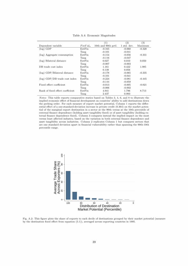
Table A.4: Economic Magnitudes

(1) (2) (3)Dependent variable FinV uls 10th and 90th pctl. 1 std. dev. Maximum(log) GDP ExtFin -0.165 -0.060 -0.320

Tang -0.101 -0.041(log) Aggregate consumption ExtFin -0.154 -0.056 -0.331

Tang -0.116 -0.047(log) Bilateral distance ExtFin 0.027 0.010 0.050

Tang -0.007 -0.003DB trade cost index ExtFin 1.161 0.422 1.985

Tang 0.139 0.056(log) GDP/Bilateral distance ExtFin -0.178 -0.065 -0.335

Tang -0.101 -0.041(log) GDP/DB trade cost index ExtFin -0.224 -0.081 -0.445

Tang -0.144 -0.059Fixed effect coefficient ExtFin -0.013 -0.005 -0.021

Tang -0.006 -0.002Rank of fixed effect coefficient ExtFin 4.941 1.796 8.713

Tang 2.437 0.993

Notes: This table reports comparative statics based on Tables 3, 4, 6, and 8 to illustrate theimplied economic effect of financial development on countries’ ability to add destinations downthe pecking order. For each measure of export market potential, Column 1 reports the differ-ential effect of a one-standard-deviation increase in private credit (0.364) on the market poten-tial of the marginal export destination in a sector at the 90th versus at the 10th percentile ofexternal finance dependence (holding asset tangibility fixed) or of asset tangibility (holding ex-ternal finance dependence fixed). Column 3 compares instead the implied impact on the mostversus least affected industry, based on the variation in both external finance dependence andasset tangibility across industries. Column 2 replicates Column 1 but compares sectors thatare one standard deviation apart in financial vulnerability rather than spanning the 90th-10thpercentile range.

020

4060

8010

0

Ave

rage

Tra

de S

hare

Acr

oss

Exp

orte

rs (

%)

020406080100

Distribution of DestinationMarket Potential (Percentile)

Fig. A.2: This figure plots the share of exports to each decile of destinations grouped by their market potential (measureby the destination fixed effect from equation (5.1)), averaged across exporting countries in 1995.

39