Embed Size (px)
Citation preview
Financial Constraints and Firm Export Behavior
Flora Bellone* Patrick Musso† Lionel Nesta‡ Stefano Schiavo§
This version: March 2009
Abstract The paper analyzes the link between financial constraints and firm export behavior exploiting a rich dataset of French firms. We use data from two main sources. The first (Enquête Annuelle d’Entreprises – EAE) is an annual survey conducted by the Ministry of Industry, which gathers balance sheet information for all manufacturing firms with at least 20 employees. The second source of information is the DIANE database published by Bureau van Dijk, which collects data on over 1 million (French) firms. DIANE contains many financial variables absent from the EAE survey. Merging the two datasets yields around 170,000 firm/year observations, stemming from an unbalanced panel of over 25,000 manufacturing enterprises followed over the period 1993 – 2005. The actual number of observations used in the empirical analysis varies according to the specific econometric exercise. Our main finding is that firms enjoying better financial health are more likely to become exporters. The result contrasts with the previous empirical literature which found evidence that export participation improves firm financial health, but not that export starters display any ex-ante financial advantage. On the contrary, we find that financial constraints act as a barrier to export participation. Better access to external financial resources increases the probability to start exporting and also shortens the time before firms decide to serve foreign customers. This finding has important policy implications as it suggests that, in presence of financial markets imperfections, public intervention can be called for to help efficient but financially constrained firms to overcome the sunk entry costs into export markets and expand their activities abroad. Keywords: Export; Firm heterogeneity; Financial constraints; Sunk costs JEL Classification: F14; G32; L25; D92
* University of Nice-Sophia Antipolis, GREDEG UMR n° 6227, e-mail: [email protected] † University of Savoie, IREGE (IMUS) and CERAM Business School, e-mail: [email protected] ‡ Observatoire Français des Conjonctures Economiques, Département de Recherche sur l’Innovation et la Concurrence (OFCE-DRIC), e-mail: [email protected] § Corresponding author. University of Trento, Department of Economics, and OFCE-DRIC, e-mail: [email protected]

1. INTRODUCTION
The paper analyzes the link between financial factors and firm export behavior exploiting a
large dataset on French manufacturing firms. There are several reasons making this a relevant
issue. With the rise of the ‘global economy’ export performance is increasingly perceived as a
key aspect of economic performance, both for firms and for the entire macroeconomic
outlook. In the meantime, academics have been paying increasing attention to firm level
studies. Wider access to firm level data, greater computational capabilities, as well as
theoretical advances that depart from the representative agent framework have led economists
to recognize that aggregate dynamics are the result of microeconomic behavior. Thus, a clear
grasp of the latter becomes crucial to understand the former and to design appropriate
policies.
In this paper we refer to export behavior in terms of both export participation and export
intensity. A vast empirical literature documents a substantial heterogeneity across firms with
respect to foreign markets penetration (ISGEP, 2008). This has mostly been explained in
terms of systematic differences between firms in productivity levels. We claim that financial
constraints represent an additional source of heterogeneity that can help to account for
different in export behavior across firms.
Our theoretical background is casted in terms of the recent ‘new-new’ trade theory
(Melitz, 2003) which emphasizes both firm heterogeneity and the relevance of sunk entry
costs into export markets.1 Once extended to allow for imperfect capital markets, these models
show that financial variables can play a key role in determining firm export behavior (Chaney,
2005; Manova, 2006). Indeed, the existence of sunk entry costs into export markets brings
about the question of the financing of such expenditures that, by their very nature, are not
matched by contemporaneous revenues. In the presence of financial market imperfections, it
may well be —and this is the main research question from which we start— that only those
firms that can successfully overcome this financial problem become exporters. In fact, this
would be consistent with the evidence of internationalized firms outperforming non exporters
in several dimensions as shown in the large literature triggered by Bernard and Jensen (1995).
Rather than supporting this prior, the scant empirical evidence on the topic suggests that
exporting improves firm access to financial markets either by reducing informational
1The assumption that entry into foreign markets involves large sunk costs is not a novelty in the trade literature: see for instance Baldwin (1988); Roberts and Tybout (1997). This assumption is supported by an expanding empirical literature (see, among others, Bernard and Wagner, 2001; Das et al., 2001; Tybout, 2001; Bellone et al., 2008b).

asymmetries or by reducing exposure to demand-side shocks through diversification (Ganesh-
Kumar et al., 2001; Campa and Shaver, 2002; Greenaway et al.,2007). In what follows we
present an evaluation of the self-selection and ex-post effects based on a large panel of French
manufacturing firms. Our contribution is twofold. First, we propose a new way to measure the
degree of financial constraint (based on the multivariate index proposed by Musso and
Schiavo, 2008), which we believe is superior to existing methodologies. Second, we shed
light on the role played by access to external financial resources in shaping firm export
behavior. In so doing, we do not limit ourselves to export participation, but we also look at
export intensity.
We can summarize our main findings as follows. First, firms starting to export display a
significant ex-ante financial advantage compared to their non exporting counterparts. This is
consistent with the idea that limited access to external financial funds may prevent firms from
selling their products abroad. Second, we do not find significant improvement in the financial
health of firms entering into export markets. Hence, in our sample foreign markets penetration
is not associated with easier access to external financial resources, contrary to the evidence
presented in other works (see for instance Greeneway et al., 2007). When we dig deeper into
the relation between financial factors and the decision to start exporting, we find that better
access to financial markets increases the probability of firm internationalization, and also
shortens the time before that happens. Finally, among the subsample of export starters, there
is a negative relationship between export intensity and financial health. Considering the
former as a proxy for the number of destinations served, our results suggest that entering
simultaneously into many different markets entails larger sunk costs and results in a
deterioration of a firm financial position.
The rest of the paper is organized as follows. We next present an overview of the literature
on financial constraints and firm export behavior. Section 3 presents the data, discusses the
shortcomings of usual strategies employed to measure financial constraints, and illustrates the
methodology adopted here. In Section 4, we test the two hypotheses that less constrained
firms self-select into exporting, and that selling abroad improves firm financial health. We
then look more in details at the role played by financial variables in shaping the decision to
export: these results are discussed in Section 5. Section 6 concludes and draws some policy
implications.

2. A GLANCE AT THE EXISTING LITERATURE
In presence of imperfect capital markets, one can figure out at least two reasons why
exporting firms should be less financially constrained than non exporting firms.
First, if firms have to incur large sunk costs to enter into export markets, then enterprises
unable to secure enough funds may have difficulties to reach foreign customers. This implies
that only less constrained firms will be able to start exporting: such an idea is formalized by
Chaney (2005) which adds liquidity constraints to a model of international trade with
heterogeneous firms (in the spirit of Melitz, 2003). In fact, the new-new trade theory
postulates that a large part of trade barriers faced by firms take the form of fixed costs to be
paid up-front. The empirical literature documents significant hysteresis effects associated with
firm export participation and interprets this as signaling the relevance of sunk entry costs: see
for instance Roberts and Tybout (1997) for Colombia, Bernard and Wagner (2001) for
Germany, Campa (2004) for Spain, Bernard and Jensen (2004) for the US. Das et al. (2001)
estimate a structural model to quantify sunk costs and conclude that entry costs into export are
substantial. In the business literature, Moini (2007) reports results form a survey among US
non exporters, where firms claim their primary obstacle to initiate an export program is the
presence of high up-front costs.
Second, the very fact of exporting could improve firm access to external financial funds.
Again there are different candidate explanations for such an effect. Exporting firms should in
principle enjoy more stable cash flows, as they benefit from international diversification of
their sales. Hence, under the assumption that international business cycles are only
imperfectly correlated, exporting reduces vulnerability to demand-side shocks. This is the
argument put forward by Campa and Shaver (2002) and Bridges and Guariglia (2008).
Alternatively, selling in international markets can be considered as a sign of efficiency and
competitiveness by domestic investors. In a context of information asymmetries —which lie
at the heart of financial markets imperfections— exporting would thus represent a clear signal
sent by the firm to external investors. Since only the best firms export —as we know very
well by the large body of empirical literature triggered by Bernard and Jensen (1995), and as
demonstrated theoretically by Melitz (2003) — then exporting represents by itself a sign of
efficiency and a costless way for creditors to assess the potential profitability of an
investment. Ganesh-Kumar et al. (2001) find that this kind of mechanism is especially
relevant in an emerging market such India, characterized by low institutional quality. Finally,
exporting is likely to open up access to international financial markets as well, at least those

pertaining to the destination countries. In anything, foreign exchanges revenues represent a
better collateral to access external funds in foreign financial markets. Once again this channel
probably applies more directly to emerging economies, as postulated by Tornell and
Westermann (2003).2
Empirically, Campa and Shaver (2002) show that investment is less sensitive to cash flow
for the group of always exporters compared to the group of never exporters. Since in presence
of perfect capital markets investment and cash flow should not be correlated, investment-cash
flow sensitivity is often regarded as a measure of financial constraints (more on this below).
Also, when the two authors consider firms that move in and out from export markets, they
find these are more constrained when they do not sell abroad. Hence, they conclude that
exporting can help firms to reduce their financial constraints. One possible weakness of the
paper lies in the fact that export intensity has no role in the play. In fact, if the diversification
and the signaling channels were actually at work, one would expect a positive correlation
between the export to sales ratio and its ability to reduce financial constraints. Yet, Campa
and Shaver fail to find such a relationship.
Two recent papers provide further evidence backing the idea that exporting exerts a
positive effect on firm financial health. Working with a large panel of UK manufacturing
firms Greeneway et al. (2007) look for a causal nexus between the two variables, and
conclude that causality runs from export to financial health. In other words, they find no
evidence in favor of the hypothesis of less constrained firms self-selecting into export
activities, but rather strong evidence of a beneficial effect of the latter on financial health.3 In
particular, they find no significant difference in the average liquidity (or leverage) ratio of
export starters and never exporting firms. On the contrary, when comparing continuous
exporters and starters, they find the former to enjoy a better average financial health over the
sample period. Hence, they conclude that exporting does improve firm financial status, since
participating to export for longer periods makes enterprises more liquid and less leveraged.
Bridges and Guariglia (2008) focus on survival among UK firms. More specifically, they
look at the interrelations between global engagement (of which export is just one possible
manifestation), financial health, and survival. They find that lower collateral and higher
2The relevance of the institutional context is witnessed by a recent work by Espanol (2006) who find exporting firms in Argentina more financially constrained than their competitors only serving the domestic market. This can be explained by the appreciation of the local currency in the early 1990s, which resulted in a profit squeeze for exporters, and weakened their balance sheets. 3We will discuss the issues related to the measurement of financial constrained in Section 3 below. For the moment, it suffices to say that Greeneway et al. (2007) use the liquidity ratio and the leverage ratio to proxy for financial constraints.

leverage do result in higher failure probabilities, but only for purely domestic firms. They
interpret this as evidence that international activities shield firms from financial constraints or,
to put it in the terminology used so far, that internationalization is beneficial from a financial
point of view.
Despite this body of literature, we claim that the issue is not fully settled yet. We base this
statement on different considerations. First, the way financial constraints are identified and
measured remains largely debated. As discussed below, the usefulness of investment cash
flow sensitivity as a measure of financial constraints is increasingly challenged and recent
theoretical works cast doubts also on other widespread proxies. Second, the role played by
export intensity has been largely disregarded so far and remains to be determined. Last, the
econometric specifications used in the literature appear not always consistent with the stated
goal of testing the relevance of self-selection into export markets and of the existence of a
beneficial effect of internationalization on firm financial health.
3. DATA AND METHODOLOGY
We use data from two main sources. Both of them collect information on French firms,
though their coverage is somehow different. The first (Enquête Annuelle d’Entreprises –
EAE) is an annual survey that gathers balance sheets information for all manufacturing firms
with at least 20 employees.4 The second source of information is the DIANE database
published by Bureau van Dijk, which collects data on over 1 million French firms. It provides
us with many financial variables absent from the EAE survey. Merging the two datasets yields
around 170,000 firm/year observations, stemming from an unbalanced panel of over 25,000
manufacturing enterprises followed over the period 1993 – 2005.
The actual number of observations used in the empirical analysis varies according to the
specific econometric exercise. When testing for self-selection effects or ex post benefits, we
restrict our attention to export starters and never exporting firms exclusively, reducing the
number of firms to 5,700 (900 when we use models with a longer lag structure, see Section 4).
The duration analysis (Section 5a) also focuses on never exporters and starters only, but the
absence of any lag in the econometric model grants us with a dataset of 12,000 firms. On the
contrary, our analysis of the decision to export (Section 5b) pools all firm types together and
4The survey is conducted by the French Ministry of Industry. The surveyed unit is the legal (not the productive) unit, which means that we are dealing with firm-level data. To investigate the role of financial constraints on growth and survival, firm, rather than plant level data seem indeed appropriate.

therefore exploits the entire dataset: there the number of observations ranges between 19,800
and 22,000.
a. Measuring financial constraints
The way financial constraints are measured is a very sensitive issue in the literature
investigating the link between financial factors and firm behavior. Theory offers only limited
guidance in this domain, so that a clear-cut consensus has still to emerge. Under perfect
capital markets, internal and external sources of financial funds should be perfectly
substitutable (Modigliani and Miller, 1958), so that the availability of internal funds should
not affect investment decisions. Yet, when a standard investment equation is augmented with
cash flow availability, the fit of the equation improves. The most common proxy for financial
constraints is thus the sensitivity of investment to cash flow. This methodology builds on
Fazzari et al. (1988) who first define firms as financially constrained or unconstrained based
on their dividend payout ratio, then show that likely constrained firms (low dividend payout)
display higher investment-cash flow sensitivity. A number of subsequent studies find
supporting evidence using different variables to identify constrained firms (see for instance
Bond and Meghir, 1994; Gilchrist and Himmelberg, 1995; Chirinko and Schaller, 1995).
On the contrary, Devereux and Schiantarelli (1990) find that larger firms (less likely to be
constrained) exhibit a higher cash flow coefficient in the regression equation, even after
controlling for sector heterogeneity. But it is only with the work by Kaplan and Zingales
(1997) that the usefulness of investment-cash flow sensitivity as a measure of financial
constraint has been definitely questioned. Since then, other authors have reported evidence of
a negative relation between investment-cash flow sensitivity and financial constraints (for
instance Kadapakkam et al., 1998; Cleary, 2006).
Alternative strategies consist of simply classifying firms according to various proxies of
informational asymmetries (as these represent the main source of financial markets
imperfections). Hence, variables such as size, age, dividend policy, membership in a group or
conglomerate, existence of bond rating, and concentration of ownership are used to capture
ways to cope with imperfect information, which hinders access to capital markets (see for
instance Devereux and Schiantarelli, 1990; Hoshi et al., 1991; Bond and Meghir 1994;
Gilchrist and Himmelberg, 1995; Chirinko and Schaller, 1995; Cleary, 2006). Other papers
(e.g. Becchetti and Trovato, 2002) use survey data where firms give a self-assessment of their
difficulty to obtain external financial funds.
The major weakness of these strategies —as already noted by Hubbard (1998) — is that
most of the criteria tend to be time invariant whereas one can imagine that firms switch
between being constrained or unconstrained depending on overall credit conditions,
investment opportunities and idiosyncratic shocks. As a further potential problem, we add that
all the abovementioned works rely on a unidimensional definition of financial constraint, i.e.
they assume that a single variable can effectively identify the existence of a constraint, which
is viewed as a binary phenomenon either in place or not. Notable exceptions are the works by
Cleary (1999), Lamont et al. (2001) and Whited and Wu (2006). The first paper derives a
financial score by estimating the probability of a firm reducing its dividend payments (viewed
as a sign of financial constraints) conditional on a set of variables that are observable also in
the case of unlisted firms. Lamont et al. (2001) build a multivariate index by collapsing into a
single measure five variables weighted using regression coefficients taken from Kaplan and
Zingales (1997). The main problem here rests with the need to extrapolate results derived
from a small sample of US firms and apply them to a larger and different population.5 Based
on a structural model, Whited and Wu (2006) use the shadow price of capital to proxy for
financial constraints.
In the paper, we experiment different measures of financial constraints. The first two are
the liquidity ratio and the leverage ratio as employed by Greeneway et al. (2007).6 We find
two main shortcomings in these measures. First, they only capture one dimension of access to
financial markets: a firm may be liquid but nonetheless present a bad financial situation; on
the other hand, strong fundamentals may compensate for a temporary shortage of liquid
assets. Second, both ratios may suffer from some endogeneity. In other words, there are no
clear-cut theoretical priors on the relation between either liquidity or leverage and financial
constraints. While liquidity is generally regarded a sign of financial health, firms may also be
forced to withhold cash by the fact that they are unable to access external funds. In fact, a
recent theoretical contribution by Almeida et al. (2004) shows that financially constrained
firms tend to hoard cash, so that liquidity would be associated with financial constraints, not
lack thereof. In a similar vein, a high leverage, while signaling potential dangers, suggests
5Furthermore, one of the variables needed to compute the index is Tobin’s Q, whose use as a proxy for investment opportunities has often been criticized. 6The liquidity ratio is defined as a firm’s current assets minus its short-term debt over total assets; the leverage ratio as a firm’s short-term debt over current assets.

also that the firm has enjoyed, at least in the recent past, wide access to external financial
funds. Hence, one could argue that highly leveraged firms are not financially constrained.7
To account for these potential problems, we build two other measures of financial health
according to the methodology first proposed by Musso and Schiavo (2008). They exploit
information coming from seven variables: size (total assets), profitability (return on total
assets), liquidity (current asset over current liabilities), cash flow generating ability8, solvency
(own funds over total liabilities), trade credit over total assets, and repaying ability (financial
debt over cash flow).9
For each variable, we scale each firm/year observation for the corresponding 2-digit
NACE sector average and then assign to it a number corresponding to the quintiles of the
distribution in which it falls.10 The resulting information for each of the seven variables (a
number ranging from 1 to 5) is then collapsed into a single index in two alternative ways: (i) a
simple sum of the seven numbers (Score A); (ii) a count of the number of variables for which
the firm/year lies in the first or second quintiles (Score B).11 In both cases the index is then
rescaled to lie on a common 1–10 range.
[Insert Table 1 here]
The correlations between the four measures of financial constraints are presented in Table 1.
Both the Pearson’s and the Spearman’s correlation coefficients are reported, respectively
below and above the main diagonal of the correlation matrix. Leverage and liquidity are
strongly negatively correlated: more liquid firms are also less leveraged, meaning that these
two measures of financial health go hand in hand. Something similar happens for the two
multivariate scores: irrespective of the way information is combined firms are ranked in a
very similar order in terms of access to external financial resources. This results in a
7A further problem is that leverage and liquidity appear as the financial variables best discriminating between exporting and non exporting firms in the sample analyzed by Greeneway et al. (2007). Therefore, one runs the risk of ending-up with some sort of a built-in relation between these two financial variables and export status (see Greeneway et al., 2005, for details on the choice of the financial variables). 8This is the maximum amount of resources that a firm can devote to self-financing, and corresponds to the French capacité d’autofinancement. 9They are selected on the basis of their performance in existing studies, and their perceived importance in determining ease of access to external financial funds. 10Sectoral averages are subtracted to account for industry-specific differences in financial variables. Furthermore, to limit the effect of outliers we trim observations lying in the top and bottom 0.5% of the distribution for each the seven variables. 11We have tried also other ways to combine the information, with identical results. Additional details are available upon request.

Spearman’s ρ correlation of 0.90, while Pearson’s correlation coefficient reaches 0.91. Hence,
Table 1 suggests that the two ratios, and the two scores provide very similar information. On
the other hand, measuring financial constraints by means of a ratio or of a multivariate index
provides us with a different picture of the phenomenon at stake. In what follows we will
concentrate on the liquidity ratio and on Score A only: both measures are increasing in
financial health (contrary to leverage), which simplifies the discussion. Results are
qualitatively unchanged if one uses the leverage ratio and Score B.12
b. Firm productivity
In the following empirical analysis we will often use measures of total factor productivity
(TFP) to control for the existing heterogeneity among firms. TFP is computed using the so-
called multilateral productivity index first introduced by Caves et al. (1982) and extended by
Good et al. (1997). This methodology consists of computing the TFP index for firm i at time t
as follows:
( ) ( )( ) ( )( )
−++−+−−+−= ∑∑∑∑
=−
=−
==−
t
nn
N
nnnntnit
N
nntnit
t
titit xxSSxxSSyyyyTFP2
11
112
1 21
21
τττττ
τττ (1)
where Yit denotes the real gross output of firm i at time t using the set of N inputs X
nit, where
input X is alternatively capital stocks (K), labor in terms of hours worked (L) and intermediate
inputs (M). Snit
is the cost share of input Xnit
in the total cost.13 Subscripts τ and n are indices
for time and inputs, respectively, upper bars denote sample means, and small letters stand for
the logs of the variables (e.g. itit Yy ln= ). This index makes the comparison between any two
firm-year observations possible because each firm’s inputs and outputs are calculated as
deviations from a reference firm. The reference firm is a hypothetical firm that varies across
industries with outputs and inputs computed as the geometric means of outputs and inputs
over all observations and input cost-based shares computed as an arithmetic mean of cost
shares over all observations.14 This non parametric measure of relative productivity has been
12This second set of results is not reported but remains available upon request. 13See Bellon et al. (2008a) for more details on the method and a full description of the variables. 14Firms are allocated to one of the following 14 two-digit industries: Clothing and footwear; Printing and Publishing; Pharmaceuticals; House equipment and furnishings; Automobile; Transportation Machinery; Machinery and Mechanical equipment; Electrical and electronic equipment; Mineral industry; Textile; Wood and paper; Chemicals; Metallurgy, Iron and Steel; Electric and Electronic components.

popularized in the export-productivity literature by the contributions of Aw et al. (2000), and
Delgado et al. (2002).
4. EXPORT AND FINANCE: SELF-SELECTION OR EX-POST BENEFIT?
We start our econometric analysis by explicitly testing the two hypotheses mentioned above,
namely that less constrained firms self-select into export, and the possibility that exporting
improves financial health.
a. Descriptive statistics
Table 2 presents descriptive statistics for the whole sample and also for different types of
firms. We classify firms according to their export status separating those which export
throughout the sample period (Continuous Exporters), those not exporting initially but
entering foreign markets between 1993 and 2005 (Export Starters), and those always serving
the domestic market only (Never Exporters).
Consistently with the large empirical literature on export and performance (see Bernard et
al., 2007, for a recent overview) we find that exporters tend to be larger and more productive,
as well as to pay higher wages. Similarly, exporting firms appear more liquid and display
easier access to external financial funds as measured by Score A. Export starters lie somewhat
in the middle of the two groups. The last column of the Table reports a F-test for equality of
means across the three groups. The F-statistics are always larger than the 1% critical values,
thus rejecting the null hypothesis of equal means across the different types of firms.
[Insert Table 2 here]
On average, continuous exporters are double the size of non exporting firms in terms of
employees, they pay salaries that are 17% higher, and are 33% more liquid. The difference
between starters and never exporters are much lower and in terms of productivity the equality
of means cannot be rejected.
b. The ex-ante financial advantage of future exporters
We start by comparing ex-ante financial health for exporters and non exporters. This tells us
whether future exporters were less financially constrained than their non exporting
counterparts even before entering foreign markets. The comparison is performed with firms
belonging to the same industry and sharing similar characteristics in terms of size and

efficiency. The econometric specification is adapted from the literature on export and
performance (Bernard and Wagner, 1997; Bernard and Jensen, 1999), where this kind of
empirical exercises are routinely performed. We focus our attention only on non exporting
firms and export starters, and compare their financial health 1 and 3 years before the latter
group begins to export. The resulting sample is comprised of 5,727 firms when we lag
observations one year (t-1), and 2169 firms when we lag observations three years (t-3).
Hence, t is the year of entry into foreign markets (in the case of export starters), while we set
it equal to the median year for never exporters (a similar solution is adopted in Bellone et al.,
2008b; ISGEP, 2008). Specifically, we estimate:
itstiitsti EXPFIN εγα +Ζ++= −− ,, (2)
where FIN is either Score A or the liquidity ratio, EXP is the dummy for export status, and Z a
vector of controls that comprises Size (captured by the log of Employment, measured in terms
of total hours worked), productivity (TFP), and a set of industry-year dummies. It must be
emphasized that equation (2) does not test for a causal relationship. Rather, it allows us to
evaluate the strength of the pre-entry premium —i.e. to see to what extent firms that export in
time t were already less financially constrained 1 and 3 years before entering foreign
markets— by means of a simple t-test on the significance of the β coefficient. Results are
presented in Table 3.
[Insert Table 3 here]
When access to financial resources is measured using of Score A, the coefficient of the export
dummy is positive and significantly different from zero both in t-1 and in t-3. Although the
point estimate for the β coefficient is larger in t -3, we cannot reject the hypothesis of the two
being equal, so that the difference in the estimated β in t-1 and t-3 is not statistically
significant. The better financial health of future exporters is less pronounced in terms of
liquidity: exporters appear more liquid one year before entry, but not 3 years before.
As discussed above, we claim that liquidity captures just one aspect of firm ability to
access external financial resources, and suffers from potential endogeneity since higher
liquidity may signal the need for the firm to hoard cash due to its difficulties in accessing
external financial funds. Therefore we give more credit to results obtained using Score A.

Overall, Table 3 suggests that firms deciding to enter into foreign markets enjoy better
financial health ex-ante.
Equation (2) is estimated using never exporters and export starters alone; moreover, we
include both successful exporters (i.e. those firms that keep exporting ever since their entry
into foreign markets) and firms that stop exporting after a few years. This reduces potential
sample selection biases and reinforces our results since it works against the hypothesis of self-
selection.
Our conclusions differ sharply from those reported in Greeneway et al. (2007): such
difference can be imputed both to the introduction of a new way to measure financial
constraints, and to the econometric methodology. In particular, while Greeneway et al. (2007)
look at the average liquidity of firms prior to entry into foreign markers, here we look at
different points in time as normally done in the literature on export and productivity (Bernard
and Jensen, 1999).
c. Detecting ex-post effects
The results from the previous Section suggest that less constrained firms tend to become
exporters. This does not rule out the possibility that internationalization further boosts firm
financial health. Here we look at the extent to which this happens while disregarding the
specific reason behind the phenomenon: this is to say that we do not ask whether it is a
diversification rather than a signaling effect that matter.
Once again we stick to an empirical specification taken from Bernard and Jensen (1999).
The idea is very simple and consists in running a regression of the change in financial
variables on initial export status and initial firm characteristics. From the previous Section we
know that exporters enjoy better access to external funds: if export participation is beneficial,
then we should observe a differential in the way financial variables move after exporting
firms have started to serve foreign markets. We focus on a subsample made of newly
internationalized firms (export starters) and purely domestic enterprises, and we estimate the
following equation:
tititiqtsti EXPFIN ,,,/,% εγβα +Ζ++=∆ ++ (3)
where , /% i t s t qFIN + +∆ identifies the growth rate of the financial variable between time t+s and
t+q computed as log differences. As before, t is the first year of export for starters, whereas it

identifies the median year of observation in case of never exporters. The coefficient β
represents the increase in the growth rate of exporting firm financial health relative to non
exporters. If export is truly beneficial then we expect β to be significantly different from zero.
[Insert Table 4 here]
As highlighted by estimated coefficients in Table 4 we do not find any evidence to support the
idea that exporting improves firm access to external financial funds. We look at the growth of
financial variables over a very short time span, namely between the first year of entry and the
following year, and also over 3- and 5-year periods. In none of the cases is the export dummy
significant. Arguably, this does not necessarily means that exporting does not affect financial
health, but simply that beneficial effects do not appear within a 5-year horizon. Data
limitations prevent us from looking at longer horizons, since we would end up with too few
observations.
Equation (3) is estimated on the sample comprising export starters and never exporting
firms only, restricting the first group to successful entrants, i.e. only those firms that do not
exit from foreign markets (this explains the drop in the number of observations when moving
from Table 3 to Table 4. Results are qualitatively unchanged if they are included: their
exclusion should make easier to find an ex post benefit since the sample is biased in favor of
the most successful firms.
In Section 2 above we have discussed two possible reasons why exporting may exert a
positive effect on firm financial health, namely a diversification effect and a signaling effect.
In both cases one could argue that the mere fact of selling part of the production above is not
sufficient to trigger those beneficial effects, but that there is a sort of threshold effect below
which export does not count. In other words, it seems natural to look at whether export
intensity plays a role in the game or not. As already mentioned, Campa and Shaver (2002) fail
to find a relation between the share of sales to foreign customers and financial constraints,
while Greeneway et al. (2007) disregard the issue.
Hence, we substitute the export dummy with the log of export intensity (defined as export
over sales). Results presented in Table 5 are qualitatively unchanged: a higher share of sales

in foreign markets is not associated with higher growth in financial health, regardless of the
way this is measured.15
Our conclusion is confirmed when we re-estimate equation (3) on a subsample comprising
only non exporting firms and those export starters characterized by an export intensity larger
than the sector median. Results (not reported) mimic those already presented in Table 4 and
therefore do not provide any support to the existence of a beneficial effect of exporting on
financial health. Thus, overall we do not find any compelling evidence that export
participation is associated with improved financial health in the years that follow entry into
foreign markets.
[Insert Table 5 here]
5. MODELLING THE DECISION TO EXPORT
Firm export behavior must ultimately be conceived as a series of decisions regarding both
participation to export markets and the firm’s commitment to international trade. These
decisions can be modeled as the outcome of a variety of factors. Heterogeneity of firm
productivity levels is the utmost explanation for the observed differences in export behavior
across firms. Because firms are heterogeneous in their productive efficiency, they all have an
idiosyncratic ability to cope with the sunk entry costs associated with exporting. Yet this may
not exhaust the explanation. The firm’s ability to access external financial resources may well
constitute another important part of the story. In this Section, we first investigate the factors
driving the decision to export in a standard binary choice framework (Roberts and Tybout,
1997; Bernard and Wagner, 2001). Then we focalize on those firms entering for the first time
foreign markets since, in presence of sunk costs, financial constraints should be particularly
relevant for first-time exporters. Finally, we look at the determinants of export intensity.
Taking stocks of our previous findings, we expect financial constraints to be an important
driver of export behavior by firms, controlling for other relevant factors such as productivity,
human capital and firm size.
15The message does not change if both the export dummy and export intensity are included among the regressors, as well as when we add additional controls such as a dummy for multi-plan firms and wage per employee.
a. The decision to export
In this Section we follow closely Roberts and Tybout (1997) and Bernard and Wagner (2001)
and estimate a reduced form econometric specification whereby the probability of exporting
at time t is considered as a function of firm characteristics at time t-1. These include firm size,
productivity, wage per employee, along with industry and year dummies. We augment this
standard specification with our two alternative measures of financial constraints, so that we
end up estimating the following equation:
ittiitititiit yearindustryFINSubsidTFPWageSizeEXP εβββββα ++++++++= −−−− 1,541,31,21,1 (4)
where the subscript i indexes firms and t, time. EXP is a dummy variable equal to 1 if firm i
exports in year t, and 0 otherwise. Size is the log of employment (total hours worked), Wage is
the log of the ratio between the firm total wage bill and the number of hours worked, TFP is
our index of relative productivity (in logs), Subsid is a dummy variable equal to 1 if the firm
has multiple business units, and 0 otherwise. FIN denotes alternatively Score A or the
Liquidity ratio.
In first instance equation (4) is estimated by means of a random effect probit model. Then,
taking stock from the previous literature that stresses the importance of hysteresis in export
markets, we augment the model with lagged export status. The dynamic specification is then
estimated again using both a random effect probit model and a Dynamic GMM estimator
(Bernard and Wagner, 2001; Greeneway et al. 2007). Results are presented in Table 6.
[Insert Table 6 here]
In the static model of Columns (1) and (2) financial variables have the expected sign and are
significant: more liquid firms are more likely to export in the next period, as well as firms
enjoying a better financial health (as measured by Score A). Results do not change when we
introduce lagged export status, suggesting that financial constraints remain a significant
determinant of export strategy also for firms that already operate in foreign markets.
However, once the lagged dependent variable is included among the regressors, potential
endogeneity biases arise, which must be taken care of. This is done by means of the panel
GMM estimator developed by Arellanoo and Bond (1991): results obtained using this
methodology are presented in Columns (5) and (6). These show that once endogeneity biases

are corrected for, past export status captures the effect of all other controls. Only size retains a
significant effect on the probability of exporting, whereas all other variables —including
financial constraints— seem irrelevant for firms that are already selling abroad.
Hence, results from Table 6, while broadly consistent with the prior of financial variables
being relevant for the decision to export, are not unambiguously supporting this intuition. The
likely cause is that in estimating equation (4) we are pooling together new exporters and firms
that already operate in foreign markets. But since the main reason why external financial
resources are relevant is because of the need to cover sunk entry costs into destination
countries, then it is likely that financial variables affect very differently first-time exporters
and firms already accustomed to selling abroad. To investigate this issue further, we now
focus our analysis only on those firms faced with the decision to start exporting for the first
time. This is done mobilizing two econometric methodologies that account for time duration
and selection biases, respectively.
b. Accounting for time duration to export markets
To model firm entry decision into foreign markets in terms of time duration is tantamount to
equating firm growth with entry into export markets. Although export is a relatively rare
activity (Bernard et al., 2007), it becomes extremely widespread for larger firms: for instance,
French data reveal that 70% of firms with more than 20 employees (with represent our unit of
analysis) will ultimately penetrate foreign markets; this proportion increases to 95% for firms
with more than 500 employees16. This suggests that entry into export markets is a necessary
—yet significant— step for growth. Hence, the relevant issue is not so much whether firms
enter into export market, but rather the time it takes for a firm to eventually start serving
foreign customers. This Section tackles this issue explicitly using discrete-time duration
models.
We estimate a duration model for grouped data following the approach first introduced by
Prentice and Gloeckler (1978). Suppose there are firms i = 1,…,N, that enter the industry at
time t = 0. The hazard rate function for firm i at time t and t = 1,...,T to start exporting is
assumed to take the proportional hazard form: qit=q
0(t)×X ',itb, where q
0 ( )t is the baseline
hazard function and Xit is a series of time-varying covariates. More precisely, let X = {Size;
Wage; TFP; Subs; FIN}, where Size stands for employment weighted by the numbers of hours
worked, Wage is the wage bill per employee in order to control for systematic differences 16Data for all firms, on the contrary, tells that less then one fifth of manufacturing firms exports, a figure well in line with the literature.
between firms in terms of human capital, TFP is total factor productivity, Subs is set to unity
if firms has one or more subsidiaries and FIN is a measure of financial constraints. In line
with the theoretical literature, a clear assumption of the empirical model is that two firms of
the same age and with similar characteristics should start exporting after the same number of
years from start-up. The discrete-time formulation of the hazard rate of first export for firm i
in time interval t is given by a complementary log logistic function such as:
( ) ( )( ){ }tXXh ititt θβ +−−= 'expexp1 (5)
where θ(t) is the baseline hazard function relating the hazard rate ( )itt Xh at the tth interval with
the spell duration (Jenkins, 1995). Importantly, our sample includes companies of different
age, which in turn may harm the estimation of the non-exporting spell. To deal with the issue
of left censoring, we augment vector X with a full vector of dummy variables controlling for
firm age. We also add a full set of year fixed effects in order to control for the business cycle.
Hence, controlling for both firm age and year-specific effects will allow us to interpret the
hazard function as the result of the mere passage of time on the probability to expand
activities abroad. Finally, we model the baseline hazard function by using the log-transformed
of θ(t), an integer counting the number of years of presence in the market. This choice is the
discrete-time counterpart of a continuous-time specification with a Weibull hazard function.17
This model can be extended to account for unobserved heterogeneity —or ‘frailty’, to
account for systematic differences between firms.18 In a way, the inclusion of unobserved
heterogeneity is a generalization of a pooled specification ignoring it. It controls for both the
omitted variable bias and measurement errors in observed survival times and regressors
(Jenkins, 1995). Suppose that unobserved heterogeneity is described by a random variable ei
independent of Xit. The proportional hazard form with unobserved heterogeneity can now be
written as:
17It is important to distinguish between the time variable θ(t) and year specific effects. Variable θ(t) is an integer counting the number of years of observations in the dataset for a specific company, and year dummies control for macro-economic shocks which pertain to all companies. Moreover, we have experimented for alternative specifications if Time, namely the semi-parametric, polynomial
specification using time together with its squared θ(t)2 and cubic values θ(t)3, and a fully non-parametric approach using duration-interval-specific dummy variables. Because this choice does not affect the conclusions, we do not report the results from these specifications, but they are available on request. 18The term ‘frailty’ comes from medical sciences where it represents the unobserved propensity to experience an adverse health event.
( ) ( )( ){ }iititt tXXh εθβ ++−−= 'expexp1 (6)
where εi is an unobserved individual-specific error term with zero mean, uncorrelated with the
X’s. Model (6) can be estimated using standard random effects panel data methods for a
binary dependent variable, under the assumption that some distribution is provided for the
unobserved term. In our case, we will assume that the εi are distributed Normal and Gamma
(see Jenkins, 1995 for more details). Note that our comments will focus on the Gamma
distribution exclusively, and other estimates are provided as robustness checks.19 Lastly, we
perform a likelihood ratio test between the unrestricted model (with unobserved
heterogeneity) and the restricted model (without unobserved heterogeneity) to test for the
relevance of unobserved frailty. The reported estimates are chosen from the log likelihood
ratio test (LR test).
[Insert Table 7 here]
The results are displayed in Table 7, where Score A and the liquidity ratio have been used as
proxies for financial constraints. The first two columns provide estimates for pooled data and
columns (3) to (6) display estimated parameters controlling for unobserved heterogeneity.20
Generally speaking, all specifications exhibit strong consistency in the direction and
significance of the parameter estimates. Since the LR test confirms the importance of
unobserved heterogeneity, we exclusively comment on the specification controlling that
controls for it.
Particularly satisfactory is the consistency and significance of the two measures of
financial constraints, despite the fact that, with a critical probability value of 7% in model (5),
Score A appears somewhat less significant. Both suggest that financially healthy firms find it
easier to start exporting. To put it differently, availability of financial resources shortens time
leading to first export. In a way, this should come as no surprise. Both the theoretical and
empirical literature insist on the sunk costs implied by the expansion of activities abroad.
19This choice is arbitrary. As of today, there is no particular reason to prefer the assumption of a Gamma-distributed frailty over the normal distributed one. This choice is mainly motivated by the fact that the Gamma distribution is particularly convenient to manipulate and has thus been the most popular. As displayed in Table 7, results under the alternative assumption are in all respect consistent with the Gamma assumption. 20In columns (3)and (4) unobserved heterogeneity is assumed to be normally distributed, while in columns (5) and (6) the assumption is a Gamma distribution.

Hence firms with stronger financial resources should be in a better position to cope with the
extra costs —with no immediate compensation— associated with first exports. One surprise
comes from the counter-intuitive sign of TFP, implying that more productive firms are less
likely to enter into export markets. Although apparently at odds with the theoretical literature
(Melitz, 2003), this results is consistent with Bellone et al. (2008b), where a U-shaped
productivity pattern is revealed for future French exporters.21 Lastly, both size and human
capital, i.e. respectively employment and wage per employee, have the expected sign. These
estimates imply that large firms intensive in human capital are more likely to go abroad.
[Insert Table 8 here]
Using model (5), Table 8 displays the estimated baseline hazard function for the
representative firm. Note that in using a discrete-time duration specification, hazard rates can
be interpreted as probabilities of entry into export markets. First, we observe that the hazard
rate function is monotonically decreasing in time. This suggests that as time goes by, firms
will find it increasingly difficult to start exporting. We observe that the probability of entry
into export markets is 35% at the year of entry into the industry, to reach 24% after year 13.
Second, Table 8 also displays the hazard function for firms located in the 1st and 9th decile of
each significant explanatory variables, holding all other firm characteristics constant. For
simplicity, we choose to comment year 5 exclusively. We observe the followings: with
respect to the first decile of the size distribution, firms located at the 9th decile are 30% more
likely to enter into export markets (the probability rises from 24 to 32%); firms paying higher
salaries (in the 9th decile of the distribution) are 7 times more likely to enter into export
markets than firms in the first decile; firms located at the 9th decile of financial constraints
(Score A) are 6% more likely to enter into export markets.
This important role for average wage suggests that the variable is probably serving as a
proxy for some unobserved firm characteristic, that are relevant in the decision to export, such
as human capital. Turning to the effect of financial constraints, its limited magnitude (+6%)
leads us to conclude that if their effect is statistically significant, its economic relevance is
somewhat limited as compared with other variables. Using the liquidity ratio of model (6), the
21The paper shows that future exporters outperform their non exporting counterparts five years prior to entry into export market. But in their preparation to first export, firm productivity is found to temporarily decrease to then recover contemporaneously with entry. The interpretation is that the benefits from sales to foreign markets accrue at the time of entry, boosting the firm’s level of productivity.

marginal effect of financial constraints on the probability of exports rises somewhat, with a
probability of exporting of 25.8% and 29.0% for firms located at the 1st and 9th decile,
respectively. Comparing these values with those of Table 8 shows strong consistency and the
conclusion that the effect of financial constraints on the probability to export is limited in
scope still holds.
To recapitulate, we find that financial constraints are a significant determinant of firm
export decision, but that as firm size, the impact of financial constraints upon the probability
of exporting is far less important than the firm’s endowment in human capital and skills. Next
Section extends the analysis to investigate the role of financial constraints on firm-level
export intensity.
c. Accounting for initial export intensity
Here, we tackle the issue of the relationship between financial constraints and export volume
at the year of entry. Because positive exports implies that non-exporters be excluded from the
sample of analysis, one must first correct for sample selection bias and depict in the
qualitative equation the probability of being an exporter. In other words, explaining firm
commitment to export markets necessarily calls for a broader investigation explaining why
firms choose to expand their activities abroad in the first place. First, firms must decide
whether to export and, conditional on this decision, they set the volume of their production to
sell abroad. We model these two decisions by means of a Heckman model as follows
( ) ististiitei υβλσβ +Χ+Χ= −−''
,'
,ˆ (7)
where i stands for firm i, t stands for year t, ei is log export intensity, X is the vector of
explanatory variables as previously defined, β is the vector of parameter of interest and υ is an
error term.22
[Insert Table 9 here]
22The Heckman specification augments the model by adding the inverse Mill’s ratio ( )''
, β̂λ sti −Χ , where 'β̂ is obtained from the first step probit regression of export decision on X', a vector of variables
describing the determinants of export entry, which may or may not be equal to X. In the present case, we set X≡X'. Parameter σ' is then used to estimate ρ, a measure of selection bias correction.

Table 9 reports the results for both the selection equation explaining the decision of entry into
export markets and the quantitative equation explaining export intensity at the time of first
export (firms exporting throughout the sample period are therefore excluded from the
analysis). Control variables are set both at time t-1 and t-3. Altogether, the qualitative
equation shows consistency with the previous results concerning wage per employee and
financial variables, whereas the role of size vanishes. Looking at the quantitative equation at
time t-1, the striking result is the switch in sign regarding financial constraints. Financially
healthy firms are more likely to enter into export markets, but conditional on this decision,
firms which commit more to international trade appear to be financially more constrained.
Since the regression analysis is performed only on export starters, export intensity
measures the share of sales shipped abroad in the first year of export. Hence, we interpret the
results as a signal that export intensity is an indirect measure of sunk entry costs into export
markets. Indeed, since these costs tend to be market-specific, high export intensity is most
likely associated with a firm entering simultaneously in several foreign markets.23
The above remarks should call for caution. Our interpretation suggests that financial
constraints suffer from an endogeneity problem yielding this negative association with export
intensity. Importantly, the endogeneity problem is essentially caused by the simultaneous
relationship between sunk costs of entry into export markets and financial health. Hence in
order to control for that, we lag all explanatory variables three years.24 We find that three
years before entry, financially healthy firms find it easier to enter into export markets, but
financial variables do not bear any relation with the choice of the share of production which
goes abroad.
To recapitulate, financial health is an important determinant of the decision to enter into
export markets made by firms. But export intensity is chosen irrespective of financial health.
The choices about the volume of export and the number of markets served are not driven by
the availability of external financial resources.
23We do not have information on the number of markets served by exporting firms in the sample. However, the (Spearman’s) correlation between export intensity and the number of export markets served —computed on a different sample of French firms— ranges between 0.53 and 0.65, thus signalling a rather strong relationship between the two variables (we thank Matthieu Crozet for providing us with this information). 24We also experimented for a five-year lag but since the results are strictly equivalent to those using a three-year lag, we report the results for a three-year lag exclusively.

6. CONCLUSION
In the last 10 years or so, a large empirical literature has emerged that studies the peculiar
characteristics of exporting firms. Two broad stylized facts emerge: exporters perform
substantially better than their non exporting competitors; there are wide cross-country
differences in firm export behavior. This paper adds to this stream of the literature by looking
at financial factors as a key determinant of firm decisions. More specifically, we investigate
whether limited access to external financial resources may prevent firms from expanding their
activities abroad, and whether internationalization has any positive effect on financial health.
We find strong evidence that less credit-constrained firms self-select into export markets
or, from a complementary point of view, that external funds are an important determinant of
firm export status. In fact, export starters display better financial health than their non
exporting competitors even before starting to operate abroad. On the contrary, the hypothesis
that internationalization leads to better access to financial markets finds no support in our
analysis. We observe that access to external financial resources is a significant but not crucial
determinant of the probability to start exporting, but we find no evidence of a positive
relationship between financial health and the share of production sold abroad. This result
corroborates the idea that the relevance of financial constraints is due to the presence of sunk
entry costs.
All in all, we conclude that our empirical analysis supports recent models of international
trade based on firm heterogeneity and sunk entry costs. In this context public intervention can
be called upon to help efficient but financially constrained firms expand their activities
abroad.
REFERENCES
Almeida, H., M. Campello and M. Weisbach (2004), ‘The Cash Flow Sensitivity of Cash’,
Journal of Finance, 59, 4, 1777-804.
Arellano, M. and S. Bond (1991), ‘Some Tests of Specification for Panel Data: Monte Carlo
Evidence and an Application to Employment Equations’, Review of Economic Studies, 58,
2, 277-97.
Aw, B., S. Chung and M. Roberts (2000), ‘Productivity and Turnover in the Export Market:
Micro-level Evidence from the Republic of Korea and Taiwan (China)’, World Bank
Economic Review, 14, 1, 65-90.

Baldwin, R. (1988), ‘Hyteresis in Import Prices: The Beachhead Effect’, American Economic
Review, 78, 4, 773-85.
Becchetti, L. and G. Trovato (2002), ‘The Determinants of Growth of Small and Medium
Sized Firms: The Role of the Availability of External Finance’, Small Business Economics,
19, 4, 291-306.
Bellone, F., P. Musso, L. Nesta and M. Quéré (2008a), ‘Market Selection along the Firm Life
Cycle’, Industrial and Corporate Change, 17, 4, 753-77.
Bellone, F., P. Musso, L. Nesta and M. Quéré (2008b), ‘The U-shaped Productivity Dynamics
of French Exporters’, Review of World Economics, 144, 4, 636-59.
Bernard, A. and B. Jensen (1995), ‘Exporters, Jobs, and Wages in U.S. Manufacturing: 1976-
1987’, Brookings Papers on Economic Activity: Microeconomics, 67-112.
Bernard, A. and B. Jensen (1999), ‘Exceptional Exporter Performance: Cause, Effect, or
Both?’, Journal of International Economics, 47, 1, 1-25.
Bernard, A. and B. Jensen (2004), ‘Why some firms export’, Review of Economics and
Statistics, 86, 2, 561-69.
Bernard, A., B. Jensen, S. Redding and P. Schott (2007), ‘Firms in International Trade’,
Journal of Economic Perspectives, 21, 3, 105-30.
Bernard, A. and J. Wagner (1997), ‘Exports and Success in German Manufacturing’,
Weltwirtschaftliches Archiv, 133, 1, 134-57.
Bernard, A. and J. Wagner (2001), ‘Export, Entry, and Exit by German Firms’, Review of
World Economics, 137, 105-23.
Bond, S. and C. Meghir (1994), ‘Dynamic Investment Models and the Firm’s Financial
Policy’, Review of Economic Studies, 61, 2, 197-222.
Bridges, S. and A. Guariglia (2008), ‘Financial Constraints, Global Engagement, and Firm
Survival in the United Kingdom: Evidence from Micro Data’, Scottish Journal of Political
Economy, 55, 4, 444-64.
Campa, J. (2004), ‘Exchange Rates and Trade: How Important is Hysteresis in Trade?’,
European Economic Review, 48, 3, 527-48.
Campa, J. and J. Shaver (2002), ‘Exporting and Capital Investment: On the Strategic Behavior
of Exporters’, Research Papers 469, IESE Business School.
Caves, D., L. Christensen and W. Diewert (1982), ‘Multilateral Comparisons of Output,
Input, and Productivity using Superlative Index Numbers’, Economic Journal, 92, 365, 73-
86.
Chaney, T. (2005), ‘Liquidity constrained exporters’, mimeo, University of Chicago.

Chirinko, R. and H. Schaller (1995), ‘Why does Liquidity Matter in Investment Equations?’,
Journal of Money, Credit and Banking, 27, 2, 527-48.
Cleary, S. (1999), ‘The Relationship between Firm Investment and Financial Status’, Journal
of Finance, 54, 2, 673-92.
Cleary, S. (2006), ‘International Corporate Investment and the Relationships between
Financial Constraint Measures’, Journal of Banking & Finance, 30, 5, 1559-80.
Das, S., M. Roberts and J. Tybout (2001), ‘Market Entry Costs, Producer Heterogeneity, and
Export Dynamics’, Working Papers 8629, National Bureau of Economic Research.
Delgado, M., J. Farinas and S. Ruano (2002), ‘Firm Productivity and Export Markets: A non-
Parametric Approach’, Journal of International Economics, 57, 2, 397-422.
Devereux, M. and F. Schiantarelli (1990), ‘Investment, Financial Factors and Cash Flow
Evidence from U.K. Panel Data’, in G. Hubbard (ed.) Information, Capital Markets and
Investment, (Chicago: University of Chicago Press), 279-306.
Espanol, P. (2006), ‘Why Exporters can be Financially Constrained in a recently Liberalised
Economy? A Puzzle based on Argentinean Firms during the 1990’s’, Proceedings of the
German Development Economics Conference, Berlin 2006 n.7, Verein für Socialpolitik,
Research Committee Development Economics.
Fazzari, S., G. Hubbard and B. Petersen (1988), ‘Financing Constraints and Corporate
Investment’, Brookings Papers on Economic Activity 1, 141-95.
Ganesh-Kumar, A., K. Sen and R. Vaidya (2001), ‘Outward Orientation, Investment and
Finance Constraints: A Study of Indian Firms’, Journal of Development Studies, 37, 4,
133-149.
Gilchrist, S. and C. Himmelberg (1995), ‘Evidence on the Role of Cash Flow for Investment’,
Journal of Monetary Economics, 36, 3, 541-572.
Good, D., M. Nadiri and R. Sickles (1997), ‘Index Number and Factor Demand Approaches
to the Estimation of Productivity’, in H. Pesaran and P. Schmidt (eds.) Handbook of
Applied Econometrics: Microeconometrics, (Oxford:Blackwell), 14-80.
Greenaway, D., A. Guariglia and R. Kneller (2005), ‘Do Financial Factors affect Exporting
Decisions?’, GEP Research Paper 05/28, Leverhulme Center.
Greenaway, D., A. Guariglia and R. Kneller (2007), ‘Financial Factors and Exporting
Decisions’, Journal of International Economics, 73, 2, 377-395.
Hoshi, T., A. Kashyap and D. Scharfstein (1991), ‘Corporate Structure, Liquidity, and
Investment: Evidence from Japanese Industrial Groups’, Quarterly Journal of Economics,
106, 1, 33-60.

Hubbard, G. (1998), ‘Capital-Market Imperfections and Investment’, Journal of Economic
Literature, 36, 1, 193-225.
International Study Group on Export and Productivity (ISGEP) (2008), ‘Understanding
Cross-Country Differences in Exporter Premia: Comparable Evidence for 14 Countries’,
Review of World Economics, 144, 4, 596-635.
Jenkins, S. (1995), ‘Easy Ways to Estimate Discrete Time Duration Models’, Oxford Bulletin
of Economics and Statistics, 57, 129-138.
Kadapakkam, P-R., P. Kumar and L. Riddick (1998), ‘The Impact of Cash Flows and Firm
Size on Investment: The International Evidence’, Journal of Banking & Finance, 22, 3,
293-320.
Kaplan, S. and L. Zingales (1997), ‘Do Investment-Cash Flow Sensitivities provide useful
Measures of Financing Constraints?’, Quarterly Journal of Economics, 112, 1, 169-215.
Lamont, O., C. Polk and J. Saa-Requejo (2001), ‘Financial Constraints and Stock Returns’,
Review of Financial Studies, 14, 2, 529-54.
Manova, K. (2008), ‘Credit Constraints, Heterogeneous Firms, and International Trade’,
Working Papers 14531, National Bureau of Economic Research.
Melitz, M. (2003), ‘The Impact of Trade on Intra-industry Reallocations and Aggregate
Industry Productivity’, Econometrica, 71, 6, 1695-1725.
Modigliani, F. and M. Miller (1958), ‘The Cost of Capital, Corporation Finance and the
Theory of Investment’, American Economic Review, 48, 3, 261-97.
Moini, A. (2007), ‘Export Behavior of Small Firms: The Impact of Managerial Attitudes’, The
International Executive, 33, 2, 14-20.
Musso, P. and S. Schiavo (2008), ‘The Impact of Financial Constraints on Firm Survival and
Growth’, Journal of Evolutionary Economics, 18, 2, 135-49.
Prentice, R. and L. Gloeckler (1978), ‘Regression Analysis of Grouped Survival Data with
Application to Breast Cancer Data’, Biometrics, 34, 57-67.
Roberts, M. and J. Tybout (1997), ‘The Decision to Export in Colombia: an Empirical Model
of Entry with Sunk Costs’, American Economic Review, 87, 4, 545-64.
Tornell, A. and F. Westermann (2003), ‘Credit Market Imperfections in Middle Income
Countries’, Working Papers 9737, National Bureau of Economic Research.
Tybout, J. (2001), ‘Plant- and Firm-Level Evidence on “New” Trade Theories’, Working
Papers 8418, National Bureau of Economic Research.
Whited, T. and G. Wu (2006), ‘Financial Constraints Risk’, Review of Financial Studies, 19,
2, 531-59.

Acknowledgments The authors blame each other for any remaining mistake. They nevertheless agree on the need to thank Sylvain Barde, Jean-Luc Gaffard, Sarah Guillou, Mauro Napoletano and Evens Salies for insightful conversations. Seminar participants at GREDEG, University of Trento, the 2nd ACE International Conference in Hong Kong, the ISGEP Workshop in Nottingham, the 12th International Schumpeter Society Conference in Rio de Janeiro, the 10th ETSG Conference in Warsaw, and the DIME Workshop ‘The dynamics of firm evolution: productivity, profitability and growth’ in Pisa provided us with valuable comments on earlier drafts.

TABLE 1 Correlations between Financial Constraints indexes
Pearson’s r and Spearman’s ρ Correlation Coefficients
Liquidity ratio Leverage ratio Score A Score B
Liquidity ratio – -0.98 0.49 0.44
Leverage ratio -0.92 – -0.53 -0.47
Score A 0.46 -0.44 – 0.90
Score B 0.41 -0.40 0.91 –
Notes: Numbers in italics denote Spearman’s ρ correlation coefficients
TABLE 2 Descriptive statistics
All Continuous Export Never
Firms Exporters Starters Exporters F-stat
Employees 88.083 115.839 59.672 56.799 1,477.65***TFP 0.997 1.003 0.990 0.992 85.57***
Wage per employee 0.103 0.107 0.099 0.091 515.14***
Score A 5.620 5.825 5.448 5.261 1,133.34***
Liquidity ratio 0.293 0.320 0.273 0.240 727.78***
Observations 167,597 85,720 63,402 18,475
TABLE 3
Self-selection into exporting by less constrained firms
Score A Liquidity ratio
s=1 s=3 s=1 s=3
(1) (2) (3) (4)
Export 0.146*** 0.228** 0.016* 0.009 [0.052] [0.094] [0.010] [0.016]
log Emplt-s 0.188*** 0.075 0.006 -0.025**
[0.041] [0.067] [0.008] [0.012]
log TFPt-s 2.794*** 2.933*** 0.347*** 0.443***
[0.142] [0.247] [0.026] [0.043]
Firms/Observations 5,727 2,169 5,727 2,169 of which: starters† 3,427 1,284 3,427 1,284
non export. 2,300 885 2,300 885
R-squared 0.111 0.159 0.073 0.132
Notes: † Including firms that later stop exporting
Standard errors in brackets
* significant at 10%; ** significant at 5%; *** significant at 1%

TABLE 4 Measuring ex-post effects
Score A Liquidity ratio
t t+1 t+1 t t+1 t+1
t+1 t+3 t+5 t+1 t+3 t+5
(1) (2) (3) (4) (5) (6)
log (Exp/Sales)t=0 -0,003 0,036 0,042 0,047 -0,057 -0,052
[0.013] [0.022] [0.034] [0.033] [0.057] [0.090]
log Emplt=0 -0,012 -0,001 0,019 -0,035 0,007 -0,003
[0.009] [0.014] [0.018] [0.026] [0.038] [0.053]
log TFPt=0 -0.185*** 0,065 -0,071 0,066 -0,198 -0,302
[0.034] [0.059] [0.083] [0.093] [0.157] [0.226]
Firms/Observations 4,387 1,823 1,152 3,307 1,448 905
of which: starters† 1,423 833 541 1,144 686 441
non export. 2,964 990 611 2,163 762 464
R-squared 0,056 0,088 0,113 0,043 0,093 0,143
Notes: † include only firms that keep exporting thereafter Standard errors in brackets * significant at 10%; ** significant at 5%; *** significant at 1%
TABLE 5. Measuring ex-post effects controlling for export intensity
Score A Liquidity ratio
t t+1 t+1 t t+1 t+1
t+1 t+3 t+5 t+1 t+3 t+5
(1) (2) (3) (4) (5) (6)
log (Exp/Sales)t=0 0.100 0.054 -0.047 -0.013 -0.166 -0.534
[0.061] [0.082] [0.120] [0.158] [0.217] [0.335]
log Emplt=0 -0.013 0.001 0.018 -0.030 0.004 -0.008
[0.009] [0.013] [0.018] [0.026] [0.038] [0.053]
log TFPt=0 -0.186*** 0.064 -0.070 0.064 -0.191 -0.289
[0.034] [0.059] [0.083] [0.093] [0.157] [0.226]
Firms/Observations 4,387 1,823 1,152 3,307 1,448 905
of which: starters† 1,423 833 541 1,144 686 441
non export. 2,964 990 611 2,163 762 464
R-squared 0,055 0,089 0,115 0,044 0,093 0,140
Notes: † Include only firms that keep exporting thereafter Standard errors in brackets * significant at 10%; ** significant at 5%; *** significant at 1%

TABLE 6.
Determinants of the decision to export
RE Probit Dynamic RE Probit Dynamic GMM
(1) (2) (3) (4) (5) (6)
log Emplt-1 0.925 0.931 0.375 0.384 0.155 0.201
[0.020]*** [0.020]*** [0.012]*** [0.012]*** [0.089]* [0.092]**
log (Wage/Empl)t-1 0.897 0.878 0.564 0.549 -0.004 0.050
[0.042]*** [0.042]*** [0.028]*** [0.028]*** [0.144] [0.141]
log TFPt-1 -0.097 0.001 -0.203 -0.097 -0.001 0.038
[0.069] [0.066] [0.049]*** [0.047]** [0.099] [0.102]
Subsidt-1 0.130 0.130 0.126 0.128 -0.130 0.212
[0.027]*** [0.027]*** [0.018]*** [0.018]*** [3.359] [2.773]
Score At-1 0.042 0.045 0.003
[0.005]*** [0.004]*** [0.012]
Liquidityt-1 0.235 0.195 -0.017
[0.029]*** [0.021]*** [0.081]
Exportt-1 1.902 1.898 0.348 0.349
[0.017]*** [0.017]*** [0.066]*** [0.067]***
Observations 134,926 134,926 134,926 134,926 108,755 108,755
Firms 22,713 22,713 22,713 22,713 19,880 19,880
of which: exporters 11,678 11,678 11,678 11,678 10,241 10,241
starters† 7,938 7,938 7,938 7,938 7,306 7,306
non export. 3,097 3,097 3,097 3,097 2,333 2,333
Sargan J-statistic 0.39 0.54
m2 1.29 1.17
Notes: † Including firms that later stop exporting Standard errors in brackets; sector and year dummies included * significant at 10%; ** significant at 5%; *** significant at 1%

TABLE 7. Estimating the hazard rate of entry into export markets
Pooled Normal RE† Gamma RE‡
(1) (2) (3) (4) (5) (6)
log Time -0.651 -0.652 -0.327 -0.340 -0.189 -0.198 [0.024]*** [0.024]*** [0.098]*** [0.096]*** [0.096]** [0.095]** log Empl. 0.103 0.106 0.172 0.172 0.226 0.226 [0.018]*** [0.018]*** [0.030]*** [0.030]*** [0.036]*** [0.036]*** log (Wage/Empl.) 0.817 0.825 0.959 0.959 1.002 1.002 [0.052]*** [0.052]*** [0.073]*** [0.072]*** [0.073]*** [0.072]*** log TFP -0.454 -0.475 -0.450 -0.465 -0.398 -0.412 [0.076]*** [0.075]*** [0.092]*** [0.090]*** [0.100]*** [0.098]*** Subsid. -0.034 -0.033 -0.054 -0.052 -0.069 -0.068 [0.041] [0.041] [0.047] [0.047] [0.050] [0.050] Score A 0.011 0.014 0.014 [0.006]* [0.007]* [0.008]* Liquidity Ratio 0.137 0.159 0.167 [0.033]*** [0.040]*** [0.042]***
Observations 35,794 35,794 35,794 35,794 35,794 35,794 Firms 12,193 12,193 12,193 12,193
of which: starters♯ 8,133 8,133 8,133 8,133
non export. 4,060 4,060 4,060 4,060
LR test § 19.82*** 19.17*** 33.05*** 33.90***
Notes: † Random Effect model with Normal distributed frailty
‡ Random Effect model with Gamma distributed frailty § Likelihood Ratio test for unobserved frailty; H0: non significant unobserved frailty
♯ Including firms that later stop exporting Standard errors in brackets; dummies for firm age, sector and year specific effects included * significant at 10%; ** significant at 5%; *** significant at 1%
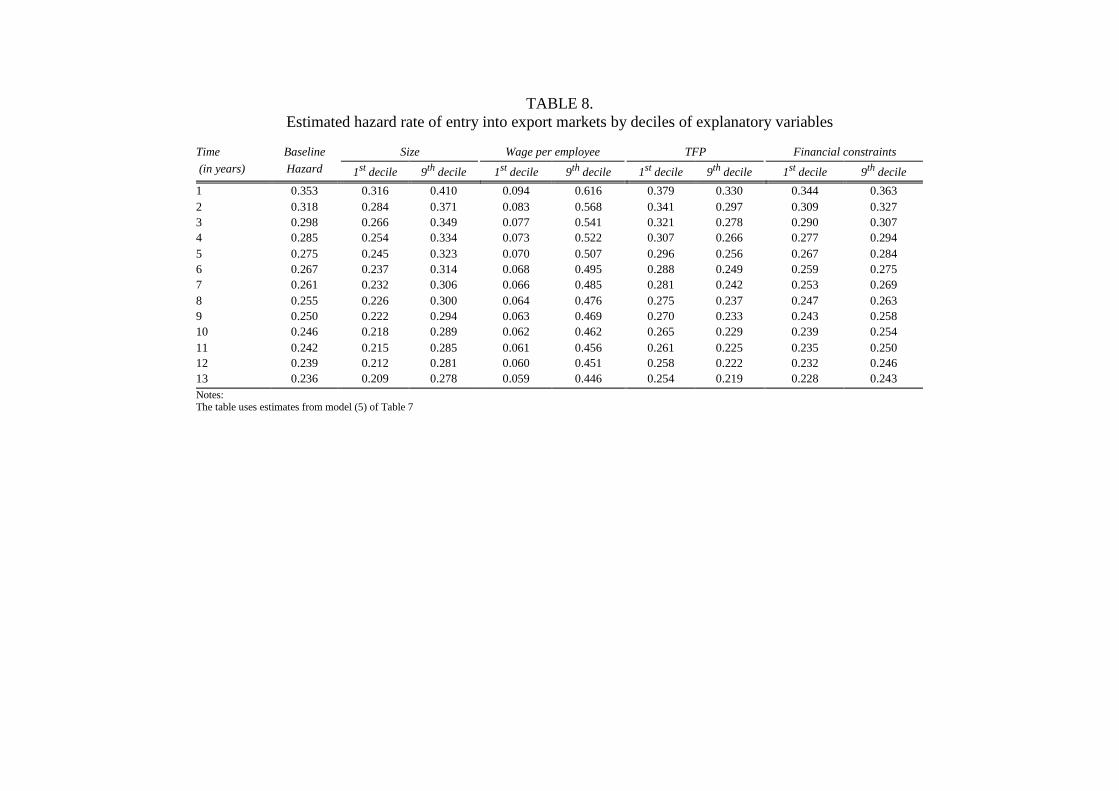
TABLE 8. Estimated hazard rate of entry into export markets by deciles of explanatory variables
Time Baseline Size Wage per employee TFP Financial constraints
(in years) Hazard 1st decile 9th decile 1st decile 9th decile 1st decile 9th decile 1st decile 9th decile
1 0.353 0.316 0.410 0.094 0.616 0.379 0.330 0.344 0.363 2 0.318 0.284 0.371 0.083 0.568 0.341 0.297 0.309 0.327 3 0.298 0.266 0.349 0.077 0.541 0.321 0.278 0.290 0.307 4 0.285 0.254 0.334 0.073 0.522 0.307 0.266 0.277 0.294 5 0.275 0.245 0.323 0.070 0.507 0.296 0.256 0.267 0.284 6 0.267 0.237 0.314 0.068 0.495 0.288 0.249 0.259 0.275 7 0.261 0.232 0.306 0.066 0.485 0.281 0.242 0.253 0.269 8 0.255 0.226 0.300 0.064 0.476 0.275 0.237 0.247 0.263 9 0.250 0.222 0.294 0.063 0.469 0.270 0.233 0.243 0.258 10 0.246 0.218 0.289 0.062 0.462 0.265 0.229 0.239 0.254 11 0.242 0.215 0.285 0.061 0.456 0.261 0.225 0.235 0.250 12 0.239 0.212 0.281 0.060 0.451 0.258 0.222 0.232 0.246 13 0.236 0.209 0.278 0.059 0.446 0.254 0.219 0.228 0.243 Notes: The table uses estimates from model (5) of Table 7

33
TABLE 9. Entry and export intensity: Heckman Two-Step model
s=1 s=3 Export Export Export Export Export Export Export Export decision intensity decision intensity decision intensity decision intensity (1) (2) (3) (4) (5) (6) (7) (8) log Emplt-s 0.047 -0.032 0.052 -0.038 0.067 -0.007 0.072 -0.02
[0.031] [0.069] [0.031]* [0.070] [0.052] [0.112] [0.052] [0.113] log TFPt-s -0.569 -0.117 -0.531 -0.214 -0.567 -0.946 -0.477 -0.936
[0.124]*** [0.373] [0.123]*** [0.355] [0.232]** [0.537]* [0.232]** [0.505]* log (Wage/Empl)t-s 0.511 0.333 0.514 0.361 0.134 0.555 0.130 0.551
[0.085]*** [0.297] [0.085]*** [0.297] [0.154] [0.303]* [0.154] [0.303]* Subsid.t-s 0.311 0.030 0.312 0.054 0.106 0.135 0.119 0.123
[0.060]*** [0.198] [0.060]*** [0.198] [0.091] [0.204] [0.091] [0.207] Score At-s 0.028 -0.059 0.044 -0.035
[0.010]*** [0.025]** [0.017]** [0.041] Liquidity ratiot-s 0.102 -0.308 0.079 -0.301
[0.054]* [0.124]** [0.099] [0.196] Firms/Observations 5727 5727 2169 2169
of which: starters† 3427 3427 1284 1284
never exporters 2300 2300 885 885
Wald c2 883.60*** 881.33*** 586.05*** 581.03***
ρ -0.169 -0.111 -0.046 -0.053 Notes: Standard errors in brackets; dummies for sector and time specific effects included * significant at 10%; ** significant at 5%; *** significant at 1% † including firms that later stop exporting