Final Report on JHT Project entitled:

Real-Time Dissemination of Hurricane Wind Fields Determined from Airborne Doppler Radar Data Real-Time Dissemination of Hurricane Wind Fields

Determined

P.I.: John F. Gamache, Hurricane Research Division (HRD) NHC/TPC Point of Contact: James Franklin

EMC Points of Contact: Naomi Surgi, Qingfu Liu

Overall goals of project: The goal of this JHT project was to transfer HRD software developed to analyze airborne

Doppler observations of hurricanes in a research framework (Gamache 1997; also see the 2003 JHT proposal for this project) to one in a “real-time” framework. The real-time version would then be able to provide information to the National Weather Service regarding winds in three dimensions near the core of the storm using the airborne Doppler radars aboard the NOAA P3 aircraft. The expertise to synthesize quality-controlled Doppler measurements into three-dimensional analyses was already well developed at HRD; however, quality control was always done manually, using analysts qualified to make judgments about which data are actually artifacts or will contribute to errors in the analysis. The analyst also had to correct many data that were badly de-aliased by the automatic processes. The analyses were also completed over a period that spanned months or years and were performed in a laboratory using computers on the ground, affording the analyst the luxury to mull over the data.

Consequently, the major tasks to be accomplished to provide real-time data were: 1) automatic quality control of radials of P3 airborne-Doppler data 2) production of analyses aboard the aircraft 3) successfully transmitting Doppler radial observations (in the form which the PI and

those receiving the data at EMC agree are most useful and practical) from the aircraft, and

4) transmitting and depicting the analyses conveniently for the very busy hurricane specialist.

The remainer of this report addresses the progress and success in performing the four

major tasks. The deliverables and metrics sections of the original proposal are also addressed briefly.

Accomplishment of Major Task No. 1—Develop automatic quality control:

The development of the quality control process has been reported on in previous reports for this project. This report discusses the quality control in its present form, as implemented aboard the NOAA P3 aircraft this year.

Description of the quality-control process: Three passes through the data are required to quality-control the data and produce wind-

field analyses. They are described in this section. First pass:

On each penetration of the storm, the observations that represent a reflection off the sea

surface must be removed. Both the main lobe and the side lobes can reflect off the sea surface and result in echo that is not from precipitation, and therefore does not measure the motion of the precipitation. These must be removed. In regions with strong, highly-reflective precipitation, the surface return will dominate only within a half-beamwidth or so of the center of the main lobe. In very weak precipitation, the echo for over a beamwidth may be dominated by sea-surface return. In regions where there is no precipitation, this region of bad data will be the largest, and it must be totally removed. Thus a simple “one size fits all” surface removal will only work if too much data are removed in a heavy precipitation situation. The result would be almost no analyzed winds at 500 m above the surface. To reduce the removal of data as much as possible, a sea-surface-reflectivity removal scheme was developed that examines both radial and azimuthal (relative to radar scan) change in reflectivity near the expected location of the sea surface. The expected location of the sea surface, and the volume expected to be dominated by its reflectivity, are determined using software modified by the PI and Mr. Peter Dodge of HRD from that reported on by Testud et al. (1996). If reflectivity increases by more than 5 dBZ per radial bin near the computed sea surface, then all data at that bin and beyond are removed. All data from the expected sea surface upward that also have a strong negative gradient with increasing height are removed. The critera used is to remove the lower bin if more than a 10 dBZ decrease in reflectivity occurs between adjacent bins on successive radials. This scheme was developed by trial and error and examining the resulting sweeps of data. After much experimentation, it appears that near the radar the scheme will keep some data down to the 150-m level, while still effectively removing the reflection of the main lobe off the sea surface. We have also developed techniques to remove the reflection of side lobes off the sea surface. The strongest manifestation of this is an annulus of contaminated data with a radius equal to the altitude of the aircraft. In regions of no or very weak precipitation, this annulus is removed automatically. If the reflectivity in this annulus is above 0 dBZ, then the ring is assumed to be dominated by reflection from precipitation and it is not removed.

In most airborne Doppler scans there are also data that are not continuous (speckles). They are usually collected at not much above the signal-to-noise ratio, or in regions where turbulence causes the spectral width of the observations to intermittently reach unacceptable levels. These “speckles,” if not removed, can reduce the effectiveness of the automatic Doppler de-aliasing (“unfolding”) software. The speckle removal appears to function well, based upon its use in many cases.

Finally, observations with a spectral velocity width of greater than a threshold value (6.25 m/s this year) are removed. Except in regions of high shear or turbulence, such observations are of low reliability, and all such observations tend to cause errors in the automatic Bargen-Brown (Bargen and Brown, 1980) de-aliasing which is the first de-aliasing method we use to pass through the velocity data. With the transmitter and signal processing used presently by the NOAA P3 Doppler radars, a spectral width threshold also effectively removes observations dominated by second-trip reflections off the sea surface.

After spurious observations are removed, the projection of aircraft motion on the radial is subtracted. The corrected observations are placed within the range of -1 to 1 times the Nyquist velocity. The Bargen-Brown algorithm is then used to de-alias (or unfold) the velocities. Bargen-Brown relies on the average of several velocities (usually 5 in 2005 season) in the bins adjacent and inward to determine the Nyquist interval in which to place the velocity measurement in question. It is initially “seeded” with the projection of the in situ wind observation made by the aircraft. This decision-making process propagates outward to the last available velocity observation on the radial. There are often gaps in observations, and in the high-velocity-gradient environment of the storm, gaps of greater than 1 km tend to cause the Bargen-Brown scheme to make errors. Thus, in each radial, no data in the initial pass are kept beyond a radial gap greater than 1 km.

The next scheme that we developed is a two-dimensional de-aliasing scheme that requires not only adjacent radial consistency, but also adjacent azimuthal (azimuth relative to radar scanning axis) consistency. Segments of radials with slowly changing velocity are separated from adjacent segments at points where there is a rapid change in radial velocity. Each segment is then compared to the adjacent previous radial to insure that the average difference of that segment from the same segment on the previous radial is less than the Nyquist velocity. This produces very consistent velocity patterns for entire sweeps.

Just as National Weather Service automatic de-aliasing may require (Eilts and Smith 1990) that de-aliased velocities fit with VAD analyses (Brown and Wexler 1968), so our automatic de-aliasing will require that the final product agree well with a low-wavenumber analysis similar to the VTD analysis of Lee et al. (1994). Thus, after passing through all these initial quality controls, the data are then interpolated to a polar grid that has an azimuthal resolution of 15 degrees, a vertical resolution of 0.5 km, and a radial resolution determined by what is allowed in memory. For most of the 2004 and 2005 cases, a radial resolution of 4 km was chosen. A three-dimensional variational synthesis of winds from the interpolated radials is then produced that has a radial resolution of 4 km, a vertical resolution of .5 km, and includes the wavenumber 0 and 1 Fourier components of radial, tangential, and vertical wind. Examples of such a wind field at the 0.5-km and 1-km level are shown in Figure 1 for the first penetration of Hurricane Katrina on 28 August 2005 (2 km horizontal resolution instead of real-time 3-5 km).

Second pass:

The entire purpose of the first pass through the data is to improve the de-aliasing used in

the second and third passes through the data. By producing such a smooth wind field, we have a way to correct for the errors that otherwise occur in the automatic de-aliasing process. In the second pass, the same decisions are made regarding sea-surface reflections, noise, and spectral width; however, the Bargen-Brown process is modified. The process still relies on the running average of previous velocities, until there is a gap in the data greater than 1 km. After the gap,

the velocities determined in the low-wavenumber analysis of pass 1 are projected on the Doppler radial. The value of the projection is then used to provide a new “seed” for the Bargen-Brown de-aliasing. This process is repeated everywhere there is a 1-km gap or greater, and there are velocities in the pass-1 analysis to “reseed” the de-aliasing process. If there are no velocities in pass 1, and there is a 1-km gap, all values in the radial beyond that radius are flagged, as in pass 1. This process allows a proper first guess to be reliably determined when the aircraft is in the eye and observing the eyewall from a distance, even where the difference between the wind speed observed at the aircraft, and the wind at the closest observation in the eyewall, may be one or two Nyquist intervals different. This process worked reliably to de-alias the winds in Hurricane Katrina while it was a category-5 hurricane on 28 August 2005.

After the enhanced Bargen-Brown de-aliasing has been performed on a sweep, the azimuthal de-aliasing technique of pass 1 is applied again. Sometimes this will produce an entire sweep that is incorrect by 2 times the Nyquist velocity, even though the sweep is internally consistent. When this occurs the average difference between the projection of the pass-1 analysis on to the sweep and the average velocities in the sweep will also be nearly 2 times the Nyquist velocity. Then the entire sweep is corrected by 2 Nyquist velocities. Finally, after all these quality controls have been applied, the data are once again compared to the pass 1 analysis, and any individual observations that differ from the wavenumber-0/1 projection by more than half a Nyquist velocity are removed. At this point, the quality control of the radials that would be sent off the aircraft for EMC is complete.

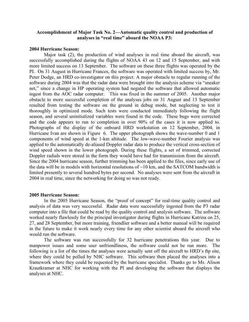
An example from an earlier analysis of the difference between a sweep that simply has the Bargen-Brown method applied to it, and a sweep that has the full de-aliasing scheme described here is shown in Fig. 2 for a sweep in Hurricane Olivia of 1994. In full disclosure, a research-quality wind field was used as substitute for the low-wavenumber field described here; however, the improvement provided by the pass-2 quality controlled is clear in this figure.

The quality-controlled radials are then used to produce a three-dimensional wind analysis. The grid used during the 2005 season was usually a 44 x 44 x 37 grid with east-west, north-south, and vertical resolutions of 4 km, 4 km, and .5 km, respectively. This is essentially the largest grid that will fit in the onboard memory, and that will allow the entire quality-control and analysis to be completed within 1 hour or so of the airborne hurricane penetration. The filtering performed in the interpolation of Doppler data is weighted more heavily in the azimuthal direction than in the radial direction to prevent significant distortion in the final Cartesian wind field. A finer-scale example of the Cartesian wind field for the same first penetration of Hurricane Katrina on 28 August 2005 is shown in Fig. 3. Besides providing a real-time analysis for the hurricane specialist to examine, the apparent quality of the analysis also provides a signal as to whether the quality control of the Doppler radial-velocity data to be sent to EMC was done properly.

Third pass:

Whenever interpolated Doppler observations are used to produce a wind field that

matches them closely, but also satisifies the discretized continuity equation, the resulting wind analysis has much lower resolution information than the original data. While the P-3 Doppler data have a radial resolution of 150 m, the real-time three-dimensional grid of pass 2 has a horizontal resolution of 3 or 4 km and a vertical resolution of .5 km, and the nature of the solution causes the actual wavelength of features resolved to be a least twice or four times that

resolution. Thus the true capability of the Doppler radar to resolve a small feature is not realized. To address this lack of full resolution, an analysis scheme was developed at HRD that allows us to see more of thie detail. It has also been modified to fit into the real-time scheme.

This new analysis type is a vertical cross-section of all three wind components along the radial flight legs. The three components are obtained without resort to the continuity equation. To accomplish this, a special grid has been developed. It uses data within 45 degrees of nadir or zenith. The radius of influence for the grid cells is 1.5 km in the radial direction (the along-track resolution that P3 fore/aft scanning is capable of), and 150 m in the vertical direction. All observations that meet the above criteria are essentially given equal weight, and it is assumed that the wind within the cell is constant throughout. There is then enough information at each grid cell to resolve the precipitation motion completely from the Doppler observations alone. A reflectivity-fall-speed relationship is used to subtract the fall speed from the precipitation motion. The result is a vertical-radial profile of winds that has 1.5 km radial resolution, and 150 m resolution. The azimuthal or cross-track resolution; however is approximately equal to twice the vertical distance of the grid cell from the flight altitude. The quality-controlled reflectivity profiles of the inbound and outbound flight legs corresponding to the same times as in Figs. 1 and 3 are shown in Fig 4. Note the lack of high reflectivity at 0 km altitude that would be present if the sea-surface had not been removed. The corresponding quality-controlled vertical profiles of total wind speed and radial wind (earth relative) for the inbound radial leg are shown in Fig. 5.

Accomplishment of Major Task No. 2—Automatic quality control and production of analyses in “real time” aboard the NOAA P3:

2004 Hurricane Season:

Major task (2), the production of wind analyses in real time aboard the aircraft, was successfully accomplished during the flights of NOAA 43 on 12 and 15 September, and with more limited success on 13 September. The software on these three flights was operated by the PI. On 31 August in Hurricane Frances, the software was operated with limited success by, Mr. Peter Dodge, an HRD co-investigator on this project. A major obstacle to regular running of the software during 2004 was that the radar data were brought into the analysis scheme via “sneaker net,” since a change in HP operating system had negated the software that allowed automatic ingest from the AOC radar computer. This was fixed in the summer of 2005. Another major obstacle to more successful completion of the analyses jobs on 31 August and 13 September resulted from testing the software on the ground in debug mode, but neglecting to test it thoroughly in optimized mode. Such tests were conducted immediately following the flight season, and several uninitialized variables were found in the code. These bugs were corrected and the code appears to run to completion in over 90% of the cases it is now applied to. Photographs of the display of the onboard HRD workstation on 12 September, 2004, in Hurricane Ivan are shown in Figure 6. The upper photograph shows the wave-number 0 and 1 components of wind speed at the 1-km altitude. The low-wave-number Fourier analysis was applied to the automatically de-aliased Doppler radar data to produce the vertical cross-section of wind speed shown in the lower photograph. During these flights, a set of trimmed, corrected Doppler radials were stored in the form they would have had for transmission from the aircraft. Since the 2004 hurricane season, further trimming has been applied to the files, since early use of the data will be in models with horizontal resolutions of ~10 km, and the SATCOM bandwidth is limited presently to several hundred bytes per second. No analyses were sent from the aircraft in 2004 in real time, since the networking for doing so was not ready. 2005 Hurricane Season:

In the 2005 Hurricane Season, the “proof of concept” for real-time quality control and analysis of data was very successful. Radar data were successfully ingested from the P3 radar computer into a file that could be read by the quality control and analysis software. The software worked nearly flawlessly for the principal investigator during flights in Hurricane Katrina on 25, 27, and 28 September, but more training, friendlier software and a better manual will be required in the future to make it work nearly every time for any other scientist aboard the aircraft who would run the software.

The software was run successfully for 32 hurricane penetrations this year. Due to manpower issues and some user unfriendliness, the software could not be run more. The following is a list of the times the analyses were actually sent off the aircraft to HRD’s ftp site, where they could be polled by NHC software. This software then placed the analyses into a framework where they could be requested by the hurricane specialist. Thanks go to Ms. Alison Krautkramer at NHC for working with the PI and developing the software that displays the analyses at NHC.

The analyses sent to NHC were:

• 5 analyses on 25 August 2005 in Hurricane Katrina • 4 analyses on 27 August 2005 in Hurricane Katrina • 5 analyses on 28 August 2005 in Hurricane Katrina • 2 analyses on 8 September 2005 in Hurricane Ophelia • 3 analyses on 9 September 2005 in Hurricane Ophelia • 5 analyses on 11 September 2005 in Hurricane Ophelia • 2 analyses on 12 September 2005 in Hurricane Ophelia • 1 analysis on 20 September 2005 in Hurricane Rita • 4 analyses on 21 September 2005 in Hurricane Rita • 1 analysis on 22 September 2005 in Hurricane Rita

Analyses of all penetrations in Hurricane Katrina, including 1 more analysis on 25

August and all 5 analyses on 29 August, were done later at a higher 2-km horizontal resolution. They have been helping hurricane specialists to understand the structure and intensity changes of Hurricane Katrina better, particularly nearly landfall. Similar higher-resolution post-flight analyses will be done for Hurricanes Ophelia and Rita.

Accomplishment of Major Task No. 3—Transmit quality-controlled Doppler radials in real-time to EMC: Production of Doppler radial files:

Unfortunately, quality-controlled Doppler radials were not sent from the P3 aircraft up to

the time of completion of this report. The trimmed quality-controlled file for each penetration was still over half a megabyte when “gzipped.” This file was designed to keep only enough radials to ensure one observation per real-time analysis grid point. In real time this ranged from 3 to 5 km. For each radial the radial resolution was 2.4 km. Even at such coarse resolution, the time to send the file from the aircraft would have been approximately a half to a full hour, assuming nothing else was using the 9600 baud channel, and assuming there were no dropouts of SATCOM. However, many other processes were competing for the bandwidth in 2005, and SATCOM dropouts occurred frequently. We expect that in the future more can be sent as the baud rates increase, and as the operational demand for quality controlled radials develops.

After the automatic Doppler processing of all data from P3 penetrations of Hurricanes in 2004, high-resolution, quality-controlled full sets of radials were made available at the Hurricane Research Division website. These high-resolution quality-controlled data sets were requested for EMC by John Waldrop. The request was that all radials be included and that the radial resolution be 150m. These quality-controlled radial data will be tested in hurricane simulations to see how they affect the results. The quality-controlled radials, in a file for each hurricane penetration, can be found at:

http://www.aoml.noaa.gov/hrd/Storm_pages/frances2004/radar.html http://www.aoml.noaa.gov/hrd/Storm_pages/ivan2004/radar.html http://www.aoml.noaa.gov/hrd/Storm_pages/jeanne2004/radar.html

Similar files will be made available in the fall of 2005 for the 2005 Hurricane Season

airborne Doppler observations.

Accomplishment of Major Task No. 4—Transmit and depict analyses for NHC hurricane specialists: 2004 Hurricane Season:

Although no files were transmitted in 2004, the entire set of penetrations for 2004 were analyzed and placed on the HRD website at: http://www.aoml.noaa.gov/hrd/Storm_pages/frances2004/radar.html http://www.aoml.noaa.gov/hrd/Storm_pages/ivan2004/radar.html http://www.aoml.noaa.gov/hrd/Storm_pages/jeanne2004/radar.html

2005 Hurricane Season:

The testing of the real-time transmission as a proof of concept went very well during the 2005 Hurricane Season. The principal investigator worked as HRD workstation scientist on NOAA 43 during the flights of 25, 27 and 28 August in Hurricane Katrina. Of all possible analyses of hurricane penetrations, 5 out of 6 were transmitted to the National Hurricane Center on 25 August, 4 out of 4 were transmitted on 27 August, and 5 out of 5 were transmitted on 28 August. Further analyses were performed and transmitted by HRD scientists Peter Dodge, Michael Black, Frank Marks, and Sim Aberson in Hurricanes Ophelia and Rita. The list of analyses sent was shown in the discussion of Major Task 2.

An example display of winds as seen at NHC is shown in Figure 7 The upper panel is a contour plot of winds in knots for the fix of Hurricane Katrina by NOAA 43 at 1755 UTC on 28 August 2005 at a level of 500 m. The lower panel shows a selection of winds as wind barbs for the same time and height level. The black barb shows the maximum wind at that level of the analysis, which was approximately 155 knots. Displays like these were available at 500 m and 1000 m for each penetration analysis sent from the aircraft. Other levels could be made available if the hurricane specialists request them in the future. Levels below 500 m are not possible, however, except in vertical cross-sections.

The vertical cross-sections from the real-time data in the same penetration are shown for the inbound and outbound legs. This year they were available from the surface to 3 km, but they could be sent for a much deeper level, to allow the forecaster to evaluate inner-core structure changes than might affect intensity. Note the much greater detail available, and the fact that data are available well below the 500 m level of the three-dimensional analysis.

The “real-time” software will be used to analyze all storm penetrations of 2005 that were observed by the NOAA P3 airborne Doppler radar. These analyses will be placed on the HRD data website as the ones for 2004 were.

Evaluation of Real-time Doppler wind fields with GPS dropsondes

The only way available to evaluate the accuracy of the real-time Doppler observations with other data is to compare them with observations made nearly concurrently with GPS dropsondes. To accomplish this the wind velocities from the three-dimensional mass-conserving analyses were mapped to the position of the GPS sondes by linear interpolation from the three-dimensional grid. The winds at the surface in the Doppler analyses were assumed to be the same as those at 500 m. The velocities from the 10-s filtered GPS winds were then compared to the real time analysis. Figure 9 shows the comparisons for all sondes dropped on 28 August 2005 in Hurricane Katrina that fell within the data coverage of the concurrent three-dimensional analyses.

The results for all comparisons on August 28th were:

• Radial wind mean difference (sonde – Doppler): -6.7 m/s -13.0 kts • Tangential wind mean difference (sonde – Doppler): -1.5 m/s -2.9 kts • Wind speed mean difference (sonde – Doppler): -0.4 m/s -0.8 kts • Radial wind RMS difference: 13.6 m/s 26.4 kts • Tangential wind RMS difference: 7.5 m/s 14.6 kts • Wind speed RMS difference: 6.4 m/s 12.4 kts

These comparisons were done only for the layer from 0 to 1 km. It should also be noted that nearly every sonde used for comparison was dropped near the radius of maximum winds. This is a region of very high wind-velocity gradients. This explains the very high RMS differences seen in the lowest 1 km. The large mean and RMS differences in radial wind show the inability of the three-dimensional analysis to resolve the low-level inflow below 500 m.

Another comparison between sondes and Doppler analyses were done for the entire set of Doppler analyses possible in the Hurricane Season of 2004. The analyses were done after the fact using the real-time Doppler software. The differences were evaluated for the entire portions of drops where there were both sonde and Doppler-wind observations. The Doppler analyses for these comparisons had a horizontal resolution of 2 km and a vertical resolution of .5 km. The analyses available for this larger comparison were for 30 August – 4 September, in Hurricane Frances, 9, 7, and 12-15 September in Hurricane Ivan, and 22 and 25 September in Hurricane Jeanne. The depth of the profiles compared ranged from 1.5 to 3 km (as opposed to 1 km or less in the first set of comparisons with real-time transmissions. The resulting comparisons for the entire 2004 Hurricane Season were:

Radial wind mean difference (sonde – Doppler): -1.4 m/s -2.7 kts Tangential wind mean difference (sonde – Doppler): 0.2 m/s 0.4 kts Wind speed mean difference (sonde – Doppler): 0.8 m/s 1.6 kts Radial wind RMS difference: 7.3 m/s 14.2 kts Tangential wind RMS difference: 6.0 m/s 11.7 kts Wind speed RMS difference: 6.2 m/s 12.1 kts

As in 2005, nearly all the drops that were made within the domain of the Doppler analyses were made near the radius of maximum wind. The variability there is quite high. All the individual sonde comparison graphs will be available at the HRD web site, and are temporarily available at:

ftp://ftp.aoml.noaa.gov/pub/hrd/gamache/2004CartesianDopplerSonde.tar. Unfortunately time has run out for this project, and this report is late. The PI plans to do

further, more systematic comparisons with sondes, including comparisons that are stratified by height of observation. We also plan to do a complete comparison for 2005. Furthermore, we plan to do a complete systematic comparison of dropsondes with the velocities seen in radial-vertical profiles. One possible comparison that might be done systematically is to search for the highest reported wind found by each eyewall sonde, and to compare these maxima with the maximum wind speed found in the vertical profiles. These comparisons will appear on the HRD website in the future.

They will also appear at: ftp://ftp.aoml.noaa.gov/pub/hrd/gamache/JHTreport The results will be in this ftp directory at least through the end of calendar year 2005.

Comparison of three-dimensional airborne Doppler wind analyses performed with manual and automatic quality control

One last test to be done is to compare the resulting wind field produced from automatic

quality control with one produced with manual quality control. An example of such an analysis is shown in Figure 11. The analyses are of wind speed at the 0.5 km level of EPAC Hurricane Guillermo observed by NOAA 43 at 0003 UTC on 3 August 1997. The clearest difference between the two methods is the smaller extent of the automatic analysis. This is unavoidable, since the automatic analysis is designed to produce as few bad analysis grid points as possible. Future work on this project could be aimed at increasing the coverage of the analysis on the inner edge of the eyewall. There are small differences in the analysis as well; however the following differences were found between the intersecting parts of the two analysis volumes:

• Mean u-component difference (auto – manual) at 0.5 km: -0.3 m/s • Mean u-component difference (auto – manual) at 1.0 km: -0.2 m/s • Mean u-component difference (auto – manual) through entire volume: -0.2 m/s • Mean v-component difference (auto – manual) at 0.5 km: 0.8 m/s • Mean v-component difference (auto – manual) at 1.0 km: 0.6 m/s • Mean v-component difference (auto – manual) through entire volume: -0.2 m/s • RMS u-component difference (auto – manual) at 0.5 km: 1.9 m/s • RMS u-component difference (auto – manual) at 1.0 km: 1.6 m/s • RMS u-component difference (auto – manual) through entire volume: 1.6 m/s • RMS v-component difference (auto – manual) at 0.5 km: 2.3 m/s • RMS v-component difference (auto – manual) at 1.0 km: 2.1 m/s • RMS v-component difference (auto – manual) through entire volume: 2.1 m/s

Thus the mean difference between the two types of analyes is well under a m/s, and the RMS vector difference is no more than about 3 m/s. The automatic quality control, although removing more data then would be preferred, did not appear to introduce marked differences in the analysis. It should be noted that is one of the examples of greater loss of coverage by the automatic mode over the manual mode. Other automatic analyses, for example in Hurricane Isabel of 2003, show that sometimes a more complete coverage of the inside edge of the eyewall occurs with automatically quality controlled data.

Deliverables

The following is a quote of the “deliverables” at the time of the proposal for this work:

1. A complete analysis in real time aboard the NOAA aircraft of the Doppler wind field.

2. A delivery of portions of this analysis in mapped form to hurricane specialists at TPC.

3. Development of input data platforms to H*Wind that are derived from the airborne Doppler wind analysis. This is a complement to the Dodge et al. JHT proposal that develops single-ground-based Doppler retrievals for H*Wind, permitting continuous incorporation of Doppler radar data into H*Wind from when the hurricane is on the high seas to when the hurricane is approaching land.

4. Prototypes of superobs, which will be developed at a further date as high-resolution models become capable of assimilating them.

Deliverable number 1 was achieved during Hurricane Ivan of 2004. At that time, due to

networking difficulties on the aircraft, there was no way to transmit the resulting analysis from the aircraft to the ground, and indeed “sneaker net” was used to get the data from the radar to the workstation to do the analysis. Sneaker net means a radar tape was read by the HRD workstation instead of a real-time file of captured ethernet radar data. A complete analysis without apparent badly de-aliased data was produced in Hurricane Ivan as shown in Fig. 6 above. Since then many real-time analyses were done in Hurricanes Katrina, Ophelia, and Rita of 2005.

Deliverable number 2 was accomplished for the first time on 25 August 2005 in Hurricane Katrina. It was accomplished 31 more times during the 2005 Hurricane Season to date.

Deliverable number 3 has been accomplished in October 2005 with the help of Mr. Nick Carrasco of HRD. It is not yet been used in H*Wind in real time, but will be evaluated over the coming months. The best way to use the Doppler data, which are not surface-wind data, will have to be determined, just as is done with flight-level data. An example of the inclusion of the data is shown in Figure 10. The panels on the right show the H*Wind analysis and data with the Doppler analyses that were actually transmitted. On the left is the operational analysis without the included Doppler analyses. Vertical-radial cross-sections may also provide aanother input platform in the future. The information in the profiles might help determine a better “real-time” reduction factor along the flight track.

Deliverable number 4 was adjusted, since it was decided provisionally that the best way to send data was to send trimmed observations of radial data that have been quality controlled. Sending the trimmed analyses allows the quality control within assimilation schemes to remove individual observations within a “superob,” and then recomputing the average. If superobs were sent, then the quality-control scheme would have to remove the entire superob, and thus eliminate the influence of all the data used to make the superob.

Trimming is needed because the data transfer will be limited. Trimming was incorporated into the software, so that presently on the aircraft, the radial resolution of included Doppler radials is 2.4 km, and the number of radials kept after trimming is enough to ensure a horizontal resolution of 3-5 km throughout the sweep.

Metrics for Success In the original proposal, three metrics for success were listed: The automatic analysis software will be considered a success if: 1. It produces an analysis very similar to that obtained with data completely

edited by human editors. 2. The analyses are available in a timely manner to hurricane specialists. 3. The specialists consider them of value in describing the wind structure of the

tropical cyclone in real time. On point 1, the agreement between the analysis from manually edited data and the

analysis from automatically quality controlled data was found to be very good. It is hoped that in the future we will be able to relax some of the conditions that lead to much more data being removed by the automatic method in some cases than is removed by manual method in the lower-reflectivity area inside the radius of maximum winds. A more complete 360o view of the eyewall from one pass through the storm might then be achieved.

Point 2--After a late start, analyses were available for Katrina. These were generally sent to the ground within an hour of the completion of the analyzed flight pattern.

The decision regarding point 3 will be up to the hurricane specialists. Another decision concerning whether these analyses indicate that work should continue on the project to send quality-controlled Doppler radials to the Environmental Modeling Center should be made by someone at EMC.

One further value for this software is its immediate forensic value. It is already being used to help decide the actual structure and intensity of Hurricane Katrina just before it make landfall, and in the coming weeks will be used in a similar manner on Hurricane Rita.

References

Bargen, D. W., and R. C. Brown, 1980: Interactive radar velocity unfolding. Proc. 19th

Conference on Radar Meteorology, Miami, Amer. Meteor. Soc., 278-283. Browning, K. A., and R. Wexler, 1968: The determination of kinematic properties of a wind

field using Doppler radar. J. Appl. Meteor., 7, 105-113. Eilts, Michael D., Steven D. Smith, 1990: Efficient dealiasing of Doppler Velocities using local

environment constraints. J. Atmos. Oceanic Technol., 7, 118-128. Gamache, John F., 1997: Evaluation of a fully-three dimensional variational Doppler analysis

technique. Preprints, 28th Conference on Radar Meteorology, Austin, TX, Amer. Meteor. Soc., 422-423.

Lee, Wen-Chau, Frank D. Marks, Jr., and Richard E. Carbone, 1994: Velocity Track Display—A technique to extract real-time tropical cyclone circulations using a single airborne Doppler radar.

Testud, Jacques, Peter H. Hildebrand, and Wen-Chau Lee, 1996: A procedure to correct airborne Doppler radar data for navigation errors using the echo returned from the Earth’s surface. J. Atmos. Oceanic Technol., 12, 800-820.

Figure 1. Wind speeds computed in quality control pass and analysis for 0.5 km (top) and 1.0 km levels. X and Y are the east-west and north-south distances from the storm center in km. Wind speeds in m/s as shown in legend

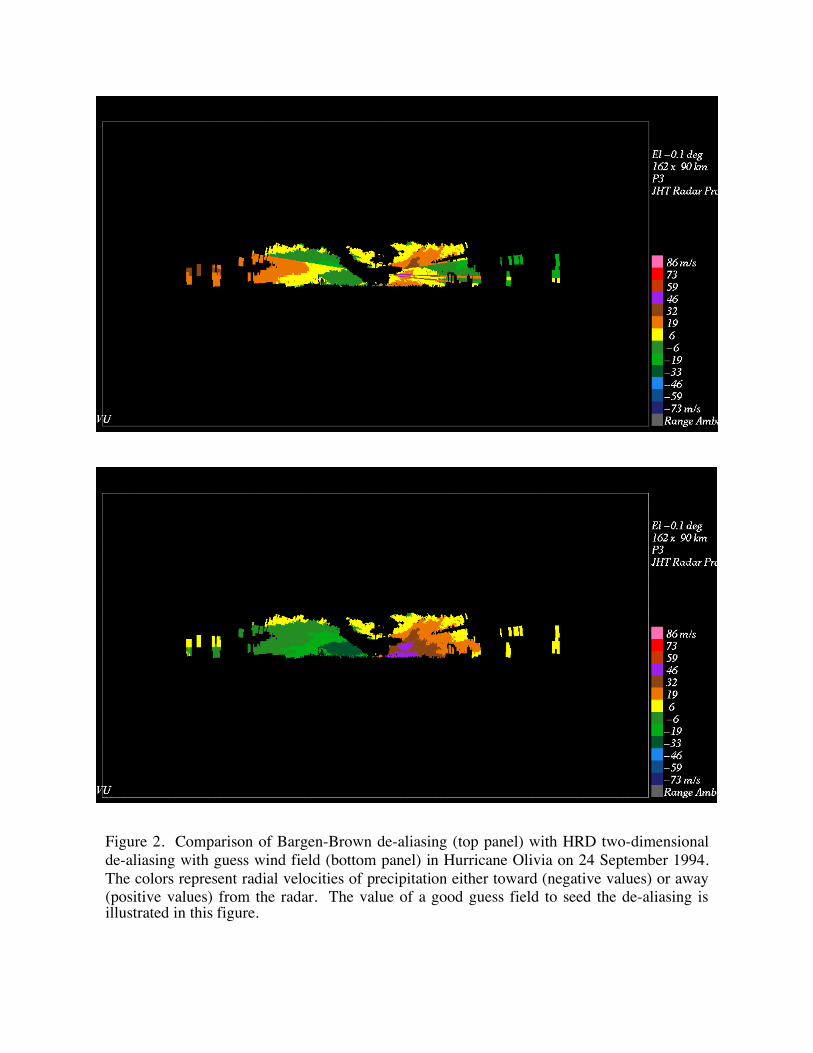
Figure 2. Comparison of Bargen-Brown de-aliasing (top panel) with HRD two-dimensional de-aliasing with guess wind field (bottom panel) in Hurricane Olivia on 24 September 1994. The colors represent radial velocities of precipitation either toward (negative values) or away (positive values) from the radar. The value of a good guess field to seed the de-aliasing is illustrated in this figure.

Figure 3. Horizontal slices of three-dimensional wind analysis produced in pass 2 of analysis and quality control system at 0.5-km (top) and 1.0-km (bottom) levels. X and Y are east-west, and north-south distances from storm center. Wind speeds in m/s as shown in legend.

Figure 4. Vertical profile of quality-controlled radar reflectivity (dbz) during inbound (top) and outbound (bottom) radial legs of the first penetration of Hurricane Katrina on 28 August 2005. Note the lack of the high reflectivity expected at the sea surface, since these data, along with the correspond radar-radial velocity data, have been removed.

Figure 5. High resolution vertical cross-sections of total windspeed on NE side of Hurricane Katrina during the first penetration from 1725 to 1818 UTC on 28 August 2005. X is radius from storm center in km. Wind speed is in m/s as shown in legend. Top panel is total wind speed, while bottom panel is radial inflow (negative) or outflow (positive). Note shallow inflow layer revealed by cross-section.

Figure 6. Digital photographs taken of HRD workstation display during the flight of NOAA 43 on 12 September 2004 in Hurricane Ivan. Top analysis shows the horizontal wind speed in m/s extending radially outward to 88 km, including wavenumbers 0 and 1 only, at 1 km flight level. Bottom analysis shows vertical cross-section of wind speed from 0.15 to 3 km in height and from 4.0 to 88 km in radius. Since these analyses were performed the radial resolution of the vertical cross-sections has been increased to 1.5 km, the resolution of the radar scans.

Figure 7. 0.5-km level wind analysis of first penetration of Hurricane Katrina on 28 August 2005, (1725-1818 UTC) as seen in the NHC displays. Upper panel shows contours of wind speed in knots, while lower panel shows wind barbs. Bold black arrow shows maximum wind at that level. Grid labels show values of latitude and longitude.

Figure 8. Vertical profiles of wind speeds in knots along the inbound and outbound radial legs flown by NOAA 43. Top panel shows the inbound profile, while bottom panel shows the outbound panel. Time shown on upper labels is for the full penetration, rather than for the respective inbound or outbound leg.

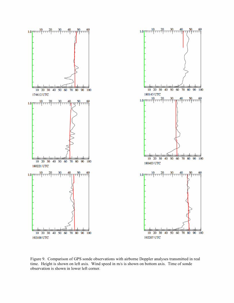
Figure 9. Comparison of GPS sonde observations with airborne Doppler analyses transmitted in real time. Height is shown on left axis. Wind speed in m/s is shown on bottom axis. Time of sonde observation is shown in lower left corner.

Figure 9 continued.

Figure9 continued.

Figure 10. H*Wind analyses for 28 August 2005 in Hurricane Katrina. Upper panels show the contours of surface wind speed. Lower panels show the data that were included in the analyses, and the extent of each type of data.

Figure 11. Comparison of wind-speed analyses of manually (top) and automatically (bottom) quality controlled data. Wind speed in m/s at 0.5 km level is shown.

References

Bargen, D. W., and R. C. Brown, 1980: Interactive radar velocity unfolding. Proc. 19th

Conference on Radar Meteorology, Miami, Amer. Meteor. Soc., 278-283. Browning, K. A., and R. Wexler, 1968: The determination of kinematic properties of a wind

field using Doppler radar. J. Appl. Meteor., 7, 105-113. Eilts, Michael D., Steven D. Smith, 1990: Efficient dealiasing of Doppler Velocities using local

environment constraints. J. Atmos. Oceanic Technol., 7, 118-128. Gamache, John F., 1997: Evaluation of a fully-three dimensional variational Doppler analysis

technique. Preprints, 28th Conference on Radar Meteorology, Austin, TX, Amer. Meteor. Soc., 422-423.

Lee, Wen-Chau, Frank D. Marks, Jr., and Richard E. Carbone, 1994: Velocity Track Display—A technique to extract real-time tropical cyclone circulations using a single airborne Doppler radar.

Testud, Jacques, Peter H. Hildebrand, and Wen-Chau Lee, 1996: A procedure to correct airborne Doppler radar data for navigation errors using the echo returned from the Earth’s surface. J. Atmos. Oceanic Technol., 12, 800-820.

Appendix

The following manual was written during Summer 2005 for the onboard scientist to run the real-time airborne Doppler quality-control and analysis software, and to send the analyses to the AOML ftp site on the ground. This manual was promised in the original proposal. The manual is actually in a fairly early stage. The software and this manual will be made more user friendly and automatic during the next year.

P3 DOPPLER-RADAR REAL-TIME INTERPOLATION AND ANALYSIS

INTRODUCTION: The software described here is designed to produce Cartesian and radial-vertical cross-sections (often referred to here as profiles) from P-3 Doppler-radar data captured in real time. HRD *.w files are produced that can be displayed for a final determination of whether the data are suitable for transmission to the ground. Small ascii text files containing a subset of these analyses are produced. They will be used to produce graphics at NHC in their NAWIPS environment. The software first interpolates to a highly smoothed, wavenumber-0 and1 polar grid, after automatic QC and dealiasing. The wavenumber-0 and 1 polar-coordinated wind field is used to produce a more effective de-aliasing, as the data are placed in a Cartesian coordinate system. This interpolation still uses a polar-coordinate weighting function. The result is a Cartesian wind field that can be displayed. The bottom two levels at .5 and 1 km are sent to the ground in the ascii files. The last part of the processing is to produce vertical profiles that do not require the continuity equation for solution, and thus have much greater detail than the full 3-D Cartesian analyses. After this processing the ascii Cartesian and vertical-radial profiles are ftp’ed to a ground computer. SYNOPSIS OF STEPS IN RADAR PROCESSING: Generating and transmitting radar analyses from the airborne radarworkstation requires these steps: Once per flight (and more if radar system crashes): Set up radar recording to single PRF, 2100-2400 pulses per second, with 2400 preferred in hurricanes. Initiate radar data capture to radar.dat by running start_radar.cmd For each penetration (in and out of the storm): 1. Run jobfile_maker to create jobfiles, based on flight track, storm position and motion. 2. Run job_auto_defreckle to create analyses and ascii data sets (for transmission)

automatically. 3. Examine analysis images with radar_slicer. 4. Ftp ascii files to ground based server. These steps are explained in more detail in the following text. After in-flight testing and experience, we hope to streamline these steps and instructions.

P3 DOPPLER-RADAR REAL-TIME INTERPOLATION AND ANALYSIS INSTRUCTIONS

1) Set radar recording parameters to single PRF. 2100 is ok for tropical storms to give a

little greater range, but if a storm has an eye, PRF should be 2400, major hurricane consider 2800 PRF. Single PRF is determined by making sure that PRF2 is equal to PRF1. To request 2400 or above you will need to reset the pulse width to its smallest size.

2) Once radar recording has begun on the P-3, run start_radar.cmd. This should be available as an icon (withouth the “.cmd” part of the name) on one of the workspaces on the HP workstation. If not, then run ./start_radar.cmd from the main hrd directory /home/hrd. This will initiate capture of radar data to the radar.dat file on /home/hrd.

3) From size of hurricane determine the outermost radius from storm center you would like to do the analysis. Be aware that for now, the maximum array size is 44x44x37. Thus if you want to go out 88 km with the storm in the center, use 88 km as the maximum radius and 4 km as the radial resolution. Take the maximum radius you want to use and divide by 22, and this will give you horizontal resolution you will have in real time. Note: if you go more than 88 km, the vertical profiles may not work due to memory problems.

4) Armed with the maximum radius information and the storm fix and motion, you should be able to answer most of the questions the jobfile maker will ask you except for transmitter related information. If you do not know the answers enter 0’s for azimuth, tilt, roll, drift, and pitch corrections, as well as 0 for the range delay. If someone has already determined these and left them in the /home/hrd directory as a param.dat file, you will have the option to use those values.

5) Check in /home/hrd to see if there are files named “radar_flt_params.dat” and “radar_analysis_params.dat”. If there are not, then see if they are in /home/hrd/workstation. If they are in /home/hrd/workstation COPY, DON’T MOVE, these files to /home/hrd.

6) In /home/hrd run ./jobfile_maker. If the “…params.dat” files do not exist there will be a much longer set of questions for you to answer. If the files exist, check to make sure the values in those files are correct or reasonable, to the best of your knowledge. If you are sure a parameter is in error follow the instructions to change that parameter. If jobfile maker bombs on you, delete these files and start from scratch below. Also remember to make sure the storm number and flight info are correct; i.e. check all the information in the menus to make sure they are correct to the best of your knowledge.

IF “params.dat” FILES DO NOT EXIST jobfile_maker answers if no param.dat files exist: Begin time is the time the aircraft was at the beginning of the inbound flight leg. Consider the maximum radius of the analysis, add 20-30 km to that, and estimate the time the aircraft was at that location. If it is a straight pass through the center figure 15 minutes earlier than the fix time for an analysis that goes out 88 km. Enter time as HHMMSS, where H M and S are the UTC hours, minutes, and seconds. End time is the time the aircraft is at the end of the outbound flight leg. Consider the maximum radius of the analysis, add 20-30 km to that, and estimate the time the aircraft was at that location. If it is a straight pass through the center figure 15 minutes later than the fix time for an analysis that goes out 88 km. If the analysis only goes out 44 km, figure about 10 minutes. Enter time as HHMMSS, where H M and S are the UTC hours, minutes, and seconds. Enter the east-west and north-south components of storm motion in m/s. Composite time should normally be the time the center was fixed. Enter the latitude and longitude of the storm when it was fixed during that pass. “Distance to go out” means the maximum radius from storm center to do the analysis. When entering this number, remember you are only allowed 22 radial bins, so if you pick 110 km, your horizontal resolution in the resulting Cartesian analyses will be 5 km. Note: if you go more than 88 km, the vertical profiles may not work due to memory problems. Enter horizontal and vertical grid resolutions for Cartesian analyses. Remember you are only allowed a box with a total number of points that is less than 44x44x37 points. Enter the vertical resolution of the radial profiles. This should usually be .15 km. Enter the ATCF storm number. If you do not know, ask the flight director or the LPS. This will be the number of the tropical cyclone for that year in the Atlantic Basin. If there have been no tropical depressions that never became tropical storms, you can get that number from the first letter of the name of the storm, for example, the ATCF number for Dennis would be 4 and for Irene would be 9. However, if there was a tropical depression that never became a tropical storm, that number must be included. If tropical depression 10 never became a tropical storm, then tropical storm Jose would have an ATCF number of 11. Your best bet is to ask the flight director, however. Next enter 0 for NOAA (varying tilt angle) antenna and 1 for French (dual fixed fore and aft pointing antennas). If you do not know, ask LPS or flight director. If you don’t know the aft azimuth and elevation (tilt) corrections enter 0 for both.

If you don’t know the range delay for the aft antenna enter 0. If you don’t know the roll, pitch or drift corrections for the aft antenna, enter 0 for each. Repeat the above 3 answers for the fore antenna. You have to repeat these answers even if it is the NOAA antenna. Enter a number between 6 and 10 for the tape drive—ignore the comment about entering a negative number for a file. Even though you are actually reading from a disk file, on the aircraft, if you open a tape with the tapeopen command (which is what the analysis software does), it will automatically open the radar.dat file and read it properly. A value of 6 to 10 will signal my software to use the tapeopen commands rather than the disk open commands, and this is correct for the HRD HP airborne workstations. If you do not know, put 1 for the first good gate, and 5 for the number of gates to average for Doppler unfolding. If you do not know enter: -99, -99, 0, 1 as suggested in the software. If you do not have a better idea, enter 6.25 for the spectral width automatic QC value. Continuity factor should be 1000. 5.5 and 2.0 are good guesses for melting band height and thickness 99 is a good default where it tells you to enter 99 100 is a good default where it tells you to enter 100 From what you know enter flight pattern estimates for inbound and outbound flight legs within 10 degrees, inbound first and then outbound. For example, if the inbound leg came in from the NE, and the outbound leg went out toward the SE, you would enter: “45, 135”. Pick a name for the Cartesian wind file. A suggested name format would be: dennis05ileg01_xy.w This name indicates hurricane dennis on the 5th day of the month, the first leg through the center of the storm and a Cartesian wind file that contains east-west, north-south, and vertical wind components. Pick a name for the vertical wind profile file. A suggested name format would be: dennis05ileg01_profile.w If you had to enter all the above information (because no “params.dat” files already existed) you are now ready to go to the section entitled: INTERPOLATION AND ANALYSIS.

IF “params.dat” FILES EXIST: IF both “params.dat” files exist, follow these instructions: Check values in “radar_flt_params.dat.” To the best of your ability, make sure the values for the listed parameters are correct. If you don’t know, leave them as they are. After finishing with the editing of “radar_flt_params.dat”: Enter a number between 6 and 10 for the tape drive—ignore the comment about entering a negative number for a file. Even though you are actually reading from a file, on the aircraft, if you open a tape with the tapeopen command (which is what the analysis software does), it will automatically open the radar.dat file and read it properly. A value of 6 to 10 will signal my software to use the tapeopen commands rather than the disk open commands, and this is correct for the HRD HP airborne workstations. Begin time is the time the aircraft was at the beginning of the inbound flight leg. Consider the maximum radius of the analysis, add 20-30 km to that, and estimate the time the aircraft was at that location. If it is a straight pass through the center figure 15 minutes earlier than the fix time for an analysis that goes out 88 km. Enter time as HHMMSS, where H M and S are the UTC hours, minutes, and seconds. End time is the time the aircraft is at the end of the outbound flight leg. Consider the maximum radius of the analysis, add 20-30 km to that, and estimate the time the aircraft was at that location. If it is a straight pass through the center figure 15 minutes later than the fix time for an analysis that goes out 88 km. If the analysis only goes out 44 km, figure about 10 minutes. Enter time as HHMMSS, where H M and S are the UTC hours, minutes, and seconds. Enter the east-west and north-south components of storm motion in m/s. Composite time should normally be the time the center was fixed. Enter the latitude and longitude of the storm when it was fixed during that pass. From what you know enter flight pattern estimates for inbound and outbound flight legs within 10 degrees, inbound first and then outbound. For example, if the inbound leg came in from the NE, and the outbound leg went out toward the SE, you would enter: “45, 135”. Pick a name for the Cartesian wind file. A suggested name format would be: dennis05ileg01_xy.w This name indicates hurricane dennis on the 5th day of the month, the first leg through the center of the storm and a Cartesian wind file that contains east-west, north-south, and vertical wind components. Pick a name for the vertical wind profile file. A suggested name format would be: dennis05ileg01_profile.w

INTERPOLATION AND ANALYSIS You should now be able to run the interpolation and analysis software. To start the process, type: ./job_auto_defreckle This should run a set of 9 routines that will produce the analyses. These routines are:

1) wind_interpolate_rt_auto_first_defreckle 2) wind_fourier_auto_first 3) indexwind_rt_fourier_auto 4) convert_rt_xy_fourier_auto 5) convert_wind_fourier_auto 6) wind_interpolate_auto_guess_fourier_defreckle 7) wind3_fill_auto_guess 8) wind_interpolate_rt_auto_guess_profile_fourier_defreckle 9) wind_rt_auto_guess_profile

In order these routines 1) interpolate data to a polar grid with the storm at the center, 2) do a wavenumber 0 and 1 fourier solution for the radial, azimuthal, and vertical winds, 3) computes polar-coordinate winds from fourier components, 4) converts polar to Cartesian wind field, 5) converts to a form “radar_slicer” can read. This file is called “first_guess_fourier_xy.w” The result from 5 is used as a guess field for dealiasing in the next 4 routines. 6) interpolates to a Cartesian grid using filtering that is polar, 7) solves for the Cartesian wind components in a Cartesian grid. Its result is the file that is named based upon your input in jobfile_maker. It also writes 4 small text files that contain the u and v wind components for the 500 and 1000 m levels. 8) interpolates to a polar grid, and 9) picks off the radius-height wind field in a vertical profile file. Its result is the file that is named based upon your input in jobfile_maker. It also writes 2 small text files that contain the wind speeds along radial cross-sections flown by the aircraft. Name examples for these 6 files are : AL09_200409121438_inbound_profile.txt AL09_200409121438_level1u.txt AL09_200409121438_level2u.txt AL09_200409121438_level1v.txt AL09_200409121438_level2v.txt AL09_200409121438_outbound_profile.txt Files with these names were created in a pass through Hurricane Ivan in 2004, and the begin time for these analyses was 1438 UTC.

CHECKING RESULTING WIND-FIELD FILES: The next step is to look at the wind fields using radar_slicer. To look at the Cartesian file type: radar_slicer dennis05ileg01_xy.w (substitute your Cartesian file name). Look at the wind field at a couple low levels (0.5 km through 1.5 km) to make sure the wind fields look realistic and appear to have been properly quality controlled. To look at the vertical cross sections you have to “play a trick” on radar_slicer. As with the Cartesian file, type “radar_slicer dennis05ileg01_profile.w”. Then pick the xz slice option. The u component is the radial component and the v component is the tangential component, DO NOT USE THE RADIAL AND TANGENTIAL BUTTONS WITH A PROFILE WIND FILE. The xz slice in this option is actually the rz slice option, since r is replaced with x in these files, and the y axis is actually the azimuthal direction in these files. When you look at the display value of y in these “xz” slices, y=15 corresponds to inbound, y=30 corresponds to outbound. If you believe the analyses to be good, look for the text files that begin with AL, have the beginning time of the analysis and end with “level1u.txt, level1v.txt, level2u.txt, and level2v.txt, or that have the correct time and either inbound or outbound in their names” You now want to ftp these to AOML. Before sending the inbound and outbound profile files, make sure to change the kmax variable from 20 to 19 in the 12th line both of those files using a text editor such as sue (microemacs), vi or pico. This has to be done manually for now. Then gzip all 6 of these text files.

FTP ftp ftp.aoml.noaa.gov login: anonymous (or I think you can use your own account to put files on my incoming directory) password: your email or something (or your own password) passive on (transfers will not work without this command) prompt bin cd hrd/incoming/gamache issue the command binary to send the files via binary “put” the 6 txt.gz files to hrd/incoming/gamache exit. Try to do this portion of the ftp correctly the first time, since you cannot change or delete files that have been placed on an “incoming” aoml ftp directory. If the transfer messes up (you are cut off in mid transfer) the only thing I can suggest is change the time in the name of the text files by one minute and try sending again. At this point you have completed the airborne processing for a given flight leg.