Final Group Report

Team RadioFreqs

Michelle Chang Michael Meegan

Gene Uehara Vlad Vakulchik

March 26, 2017

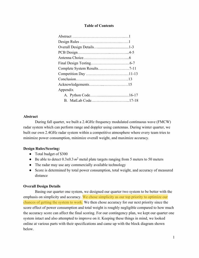
Table of Contents

Abstract …………………………………..…1 Design Rules …………………………..……1 Overall Design Details…................................1-3 PCB Design……………………..…………...4-5 Antenna Choice……………………………...6 Final Design Testing…………………………6-7 Complete System Results……………………7-11 Competition Day ……………………………11-13 Conclusion…………………………………..13 Acknowledgements………....………………15 Appendix

A. Python Code……................................16-17 B. MatLab Code………………………...17-18

Abstract

During fall quarter, we built a 2.4GHz frequency modulated continuous wave (FMCW) radar system which can perform range and doppler using cantennas. During winter quarter, we built our own 2.4GHz radar system within a competitive atmosphere where every team tries to minimize power consumption, minimize overall weight, and maximize accuracy. Design Rules/Scoring:

● Total budget of $300 ● Be able to detect 0.3x0.3 metal plate targets ranging from 5 meters to 50 metersm2 ● The radar may use any commercially available technology ● Score is determined by total power consumption, total weight, and accuracy of measured

distance Overall Design Details

Basing our quarter one system, we designed our quarter two system to be better with the emphasis on simplicity and accuracy. We chose simplicity as our top priority to optimize our chances of getting the system to work. We then chose accuracy for our next priority since the score effect of power consumption and total weight is roughly negligible compared to how much the accuracy score can affect the final scoring. For our contingency plan, we kept our quarter one system intact and also attempted to improve on it. Keeping these things in mind, we looked online at various parts with their specifications and came up with the block diagram shown below.

1

Fig 1. Block Diagram

In order to calculate the gain of the transmitting and receiving power, we used ADIsim to simulate the theoretical values. We obtained a theoretical transmitting power of 20.7 dBm and a theoretical receiving power of -90 dBm. The simulations for the transmitter and receiver are shown below.

Fig 2. Transmitter Simulation

2

Fig 3. Receiver Simulation

The table below shows the components and its model number that we selected for the final design.

Table 1. Component List

Component Model #

VCO ROS-2536C-119+

Splitter Mini SP-2U1+

Amplifier for Transmitting MMG20241H

Amplifier for Receiving MGA-13316

Mixer SIM-63LH+

Low Pass Filter LTC1563

Attenuator HMC655LP2E

PCB Design

3

After selecting the components, we began designing the PCBs according to the schematics which were provided on the component’s data sheet. Shown below are the RF and baseband schematics as well as the layouts. We made sure to align the pin headers on both boards so we can stack the RF board on top of the baseband board, making the overall system compact and durable.

Fig 4. Baseband Schematic

Fig 5. RF Schematic

4

Fig 6. Baseband Layout

Fig 7. RF Layout

5

Figure 8. Assembled PCBs Antenna Choice

When selecting the antenna, we made sure to obtain one with high gain in order to maximize the received signal. Because of this, we decided to pick an antenna with high directivity as we know that our targets are not dispersed and we care more for gain to allow for far distance measuring. This led us to purchase a Yagi antenna from Kent Electronics at wa5vjb.com as it provided a max signal of 10-11dBi at 2.4 to 2.45GHz. Below shows the antenna specification sheet which is accessible on Kent Electronic’s website at http://www.wa5vjb.com/pcb-pdfs/Yagi2400.pdf

Fig 9. Antenna Specification Sheet Final Design Testing Shown below are the individual testing of the components. LPF

6

Fig 10. LPF Demonstration LPF 3dB

Fig 11. LPF Cutoff Complete System Results

We began by testing inside the lab room and also in the Kemper hallway. We found that we were getting results with a maximum distance reading of roughly 12 meters in the hallway but we noticed a good amount of noise was prevalent in our results which led us to test outside. Figure 12 shows the noisy hallway results which is most likely due to reflection.

7

Fig 12. First Test Results We expected better results even when testing in the hallway and this led us to notice that the low noise amplifier was not working properly on our PCB. We found the problem was caused by two unconnected nodes and so as a quick fix, we directly attached two LNAs which were used in quarter one at our receiving side. We then tested our system outside using a power supply giving 8 volts. The only purpose of the 8V supply was to provide a regulated 5V input to the rest of the system, however we decided that the battery pack was stable enough to power everything, so we choose to bypass the voltage regulator and directly power our system using the provided battery pack. Using the battery pack provided mobility and greater simplicity to the system. We then made the rookie mistake of having our system on the ground when testing which led to little to no results. The reflection off the concrete and grass when the radar was placed on the ground over powered any signal we wanted to read. After making the realization that the system needed to be elevated, we measured a maximum distance of 35 meters. Figure 13 shows the results we obtained in the field. The range in this plot is not calibrated correctly as the 0 meter position should be placed at where the yellow lines end which is at around 15 meters on this plot. This test also only utilized the cantennas as the Yagi antennas were not working properly at the time of the test.

8

Figure 13. Outside Field Test In an attempt to fix the unwanted yellow lines, we managed to find the MATLAB code which does the exact same processing as the Python code. We noticed that when the MATLAB code ran, the results were much more visible and provided no unwanted yellow lines. The only downside to this method was the processing time was much longer but we decided to utilize the MATLAB code from that point on as the better visibility of our radar results outweighed the con of having to wait an extra minute. After multiple tests, we finally arrived to the conclusion that the best configuration for our system was to use the cantenna as the transmitting antenna and use the Yagi antenna as the receiving antenna. After even more tests and calibrations, we also figured out that one extra LNA being attached to our receiving side provided us with the most optimal results. Shown below are results from our testing.

9

Figure 14. Matlab Code Test Run at 30 - 40 Meters This test shows the measurement of someone walking back and forth between the 30 meter and 40 meter mark. After calibration, we were able to get accurate measurements with an error of about one meter.

10

Figure 15. Measurement Showing Max Range of Near 100 Meters This is our maximum range test and we were able to measure roughly 90 meters before the signal strength was too weak for us to make out any readings. Competition Day

During the day of the competition we were able to get readings for all the targets. The final weight of the system was 390 grams with a 1.2 W power consumption. The readings are weaker than we had hoped, however, we were still able to discern the signal from the background. Maximum range was removed from the competition. We took separate measurements for each target for a total of 5 measurements. We then processed the audio files with MatLab and compared the RTI without clutter rejection and RTI with 2-pulse canceler clutter rejection plots to find the distance of the target.

It had rained the day earlier so the water on the grass may have affected the clarity of the desired signal. Maximum range, however, was removed from the competition, so the drop in performance ultimately did not matter. Figure # shows the final configuration of the system with the housing.

11

(a)

(b) Figure 16. Final Testing Configuration

(a) (b)

12

(c) (d)

(e) Figure 17. Competition Day Results Conclusion

Overall, we learned that constructing a fully working radar system involves meticulous attention to detail and a good amount of luck. From purchasing enough components to connecting every node during PCB layout to debugging the complete system, we all agreed that the project, without a doubt, was an immense learning experience as problems we could have never predicted came up during the process. Minimal fixes such as testing the complete system outside instead of inside proved to greatly improve the measurements.

The real life application of this radar is limited as we did not process the data in real time. We could further improve the usability of the radar if we had on-board processing and a display to see the measurements as they occur. Course Suggestions

13

● Reference exemplified final reports during quarter one labs in order to mitigate problems that can arise in quarter two and get students more familiar with the entire system. Although we knew about the reports, we did not refer to them until quarter two. One possibility is to provide final report URLs in quarter one prelabs for students to view.

● Give the recommendation of purchasing at least three times the amount of components since each team will usually receive three PCBs and all PCBs may need to be soldered. It is usually cheaper to buy in bulk so there is not too big of a downside to doing this.

Bill of Materials

14

Acknowledgements Professor Xiaoguang Liu TAs: Daniel Kuzmenko, Hao Wang, Songjie Bi Team 3061 (2015-2016) Sean Huang

15

Appendix A - Python Code # -*- coding: utf-8 -*- #range radar, reading files from a WAV file # Originially modified by Meng Wei, a summer exchange student (UCD GREAT Program, 2014) from Zhejiang University, China, from Greg Charvat's matlab code # Nov. 17th, 2015, modified by Xiaoguang "Leo" Liu, lxgliu@ucdavis.edu import wave import os from struct import unpack import numpy as np from numpy.fft import ifft import matplotlib.pyplot as plt from math import log #constants c= 3E8 #(m/s) speed of light Tp = 20E-3 #(s) pulse duration T/2, single frequency sweep period. fstart = 2260E6 #(Hz) LFM start frequency fstop = 2590E6 #(Hz) LFM stop frequency BW = fstop-fstart #(Hz) transmit bandwidth trnc_time = 0 #number of seconds to discard at the begining of the wav file window = False #whether to apply a Hammng window. # for debugging purposes # log file #logfile = 'log_new.txt' #logfh = open(logfile,'w') #logfh.write('start \n') #read the raw data .wave file here #get path to the .wav file #filename = os.getcwd() + '\\running_outside_20ms.wav' filename = os.getcwd() + '\\range_test2.wav' # The initial 1/6 of the above wav file. To save time in developing the code #open .wav file wavefile = wave.open(filename, "rb") # number of channels nchannels = wavefile.getnchannels() # number of bits per sample sample_width = wavefile.getsampwidth() # sampling rate Fs = wavefile.getframerate() trnc_smp = int(trnc_time*Fs) # number of samples to discard at the begining of the wav file

# number of samples per pulse N = int(Tp*Fs) # number of samples per pulse # number of frames (total samples) numframes = wavefile.getnframes() # trig stores the sampled SYNC signal in the .wav file #trig = np.zeros([rows,N]) trig = np.zeros([numframes - trnc_smp]) # s stores the sampled radar return signal in the .wav file #s = np.zeros([rows,N]) s = np.zeros([numframes - trnc_smp]) # v stores ifft(s) #v = np.zeros([rows,N]) v = np.zeros([numframes - trnc_smp]) #read data from wav file data = wavefile.readframes(numframes) for j in range(trnc_smp,numframes): # get the left (SYNC) channel left = data[4*j:4*j+2] # get the right (Data) channel right = data[4*j+2:4*j+4] #.wav file store the sound level information in signed 16-bit integers stored in little-endian format #The "struct" module provides functions to convert such information to python native formats, in this case, integers. if len(left) == 2: l = unpack('h', left)[0] if len(right) == 2:

r = unpack('h', right)[0] #normalize the value to 1 and store them in a two dimensional array "s" trig[j-trnc_smp] = l/32768.0 s[j-trnc_smp] = r/32768.0 #trigger at the rising edge of the SYNC signal trig[trig < 0] = 0; trig[trig > 0] = 1; #2D array for coherent processing s2 = np.zeros([int(len(s)/N),N]) rows = 0; for j in range(10, len(trig)): if trig[j] == 1 and np.mean(trig[j-10:j]) == 0: if j+N <= len(trig): s2[rows,:] = s[j:j+N] rows += 1

16

s2 = s2[0:rows,:] #pulse-to-pulse averaging to eliminate system performance drift overtime for i in range(N): s2[:,i] = s2[:,i] - np.mean(s2[:,i]) #2pulse cancelation s3 = s2 for i in range(0, rows-1): s3[i,:] = s2[i+1,:] - s2[i,:] rows = rows-1 s3 = s3[0:rows,:] #apply a Hamming window to reduce fft sidelobes if window=True if window == True: for i in range(rows): s3[i]=np.multiply(s3[i],np.hamming(N)) ##################################### # Range-Time-Intensity (RTI) plot # inverse FFT. By default the ifft operates on the row v = ifft(s3) #get magnitude v = 20*np.log10(np.absolute(v)+1e-12) #only the first half in each row contains unique information v = v[:,0:int(N/2)] #normalized with respect to its maximum value so that maximum

is 0dB m=np.max(v) grid = v grid=[[x-m for x in y] for y in v] # maximum range max_range =c*Fs*Tp/4/BW # maximum time max_time = Tp*rows plt.figure(0) plt.imshow(grid, extent=[0,max_range,0,max_time],aspect='auto', cmap =plt.get_cmap('gray')) plt.colorbar() plt.clim(0,-100) plt.xlabel('Range[m]',{'fontsize':20}) plt.ylabel('time [s]',{'fontsize':20}) plt.title('RTI with 2-pulse clutter rejection',{'fontsize':20}) plt.tight_layout() plt.show() #plt.subplot(612) #plt.plot(grid[5]) #plt.subplot(613) #plt.plot(grid[6]) #plt.subplot(614) #plt.plot(grid[20]) # #plt.subplot(615) #plt.plot(grid[30]) #plt.subplot(616) #plt.plot(grid[40])

Appendix B MATLAB Code %MIT IAP Radar Course 20112.5 %Resource: Build a Small Radar System Capable of Sensing Range, Doppler, %and Synthetic Aperture Radar Imaging % %Gregory L. Charvat %Process Range vs. Time Intensity (RTI) plot tic clear all; close all; % read the raw data .wav file here % replace with your own .wav file [Y,FS] = audioread('win3040.wav'); dbv=@(x) 20*log10(abs(x)); %constants

c = 3E8; %(m/s) speed of light %radar parameters Tp = 20E-3; %(s) pulse time N = Tp*FS; %# of samples per pulse fstart = 2260E6; %(Hz) LFM start frequency fstop = 2590E6; %(Hz) LFM stop frequency BW = fstop-fstart; %(Hz) transmti bandwidth f = linspace(fstart, fstop, N/2); %instantaneous transmit frequency %range resolution rr = c/(2*BW); max_range = rr*N/2; %the input appears to be inverted trig = -1*Y(:,1); s = -1*Y(:,2); clear Y;

17

%parse the data here by triggering off rising edge of sync pulse count = 0; thresh = 0; start = (trig > thresh); for ii = 100:(size(start,1)-N) if start(ii) == 1 && mean(start(ii-99:ii-1)) == 0 %start2(ii) = 1; count = count + 1; sif(count,:) = s(ii:ii+N-1); time(count) = ii*1/FS; end end %check to see if triggering works % plot(trig,'.b'); % hold on;si % plot(start2,'.r'); % hold off; % grid on; %subtract the average ave = mean(sif,1); for ii = 1:size(sif,1); sif(ii,:) = sif(ii,:) - ave; end zpad = 8*N/2; %RTI plot figure(10); v = dbv(ifft(sif,zpad,2));

S = v(:,1:size(v,2)/2); m = max(max(v)); imagesc(linspace(0,max_range,zpad)*0.77,time,S-m,[-80, 0]); colorbar; ylabel('time (s)'); xlabel('range (m)'); title('RTI without clutter rejection'); xlim([0, 110]) set(gca, 'YDir', 'normal') set(gca, 'XTick', 0:10:110) %2 pulse cancelor RTI plot figure(20); sif2 = sif(2:size(sif,1),:)-sif(1:size(sif,1)-1,:); v = ifft(sif2,zpad,2); S=v; R = linspace(0,max_range,zpad); for ii = 1:size(S,1) %S(ii,:) = S(ii,:).*R.^(3/2); %Optional: magnitude scale to range end S = dbv(S(:,1:size(v,2)/2)); m = max(max(S)); imagesc(R*0.77,time,S-m,[-80, 0]); colorbar; ylabel('time (s)'); xlabel('range (m)'); xlim([0, 110]); set(gca, 'YDir', 'normal') set(gca, 'XTick', 0:10:110) title('RTI with 2-pulse cancelor clutter rejection'); toc

18