Field Tests and Analyses of Concrete Pavement in Texarkana ... · FIELD TESTS AND ANALYSES OF CONCRETE PAVEMENT May 1994 IN TEXARKANA AND LA PORTE, TEXAS 6. Performing Organization

TECHNICAL REPORT DOCUMENTATION PAGE

1. Report No. 2. Government Accession No. 3. Recipient's Catalog No.

FHW A/TX-94/1244-7

4. Title and Subtitle S. Report Date

FIELD TESTS AND ANALYSES OF CONCRETE PAVEMENT May 1994 IN TEXARKANA AND LA PORTE, TEXAS 6. Performing Organization Code

7. Author(s) 8. Performing Organization Report No.

Tianxi Tang, Dan G. Zollinger, and B. Frank McCullough Research Report 1244-7

9. Performing.Organization Name and Address 10. Work Unit No. (TRAIS)

Texas Transportation Institute The Texas A&M University System 11. Contract or Grant No. College Station, Texas 77843-3135 Study No. 0-1244

12. Sponsoring Agency Name and Address 13. Type of Report and Period Covered

Texas Department of Transportation Interim: Research and Technology Transfer Office September 1989-December 1992 P. 0. Box 5080 14. Sponsoring Agency Code Austin, Texas 78763-5080

15. Supplementary Notes

Research performed in cooperation with the Texas Department of Transportation and the U.S. Department of Transportation, Federal Highway Administration Research Study Title: Evaluation of the Performance of Texas Pavements Made with Different Coarse Aggregates

16. Abstract

This report summarizes the research results obtained from two field tests for Portland cement concrete pavements. One field test was carried out on test sections of jointed plain concrete pavement in Texarkana, Texas, and the other was carried out on test sections of continuously reinforced concrete pavement in La Porte, Texas. Laboratory tests and theoretical analysis were also performed to help in understanding and analyzing the field observation. A close-form solution is proposed for thermal stresses in a concrete slab when it is curled up. This solution is for the case where the temperature decrease in the concrete slab exce.eds a limit so that a gap between the slab and foundation forms. This case was not addressed in the Westergaard solution. Fracture tests were applied to the concrete made with different coarse aggregates used for Texas pavements and have shown that fracture mechanics is a powerful tool to judge the quality of the pavement. With these efforts, a method based on fracture mechanics is proposed to determine the depth and spacing of the jointed plain concrete pavement. This method has successfully been applied to the test section in Texarkana.

17. KeyWords 18. Distribution Statement

Aggregates, Concrete, Creep, Curing Methods, No restrictions. This document is available Fracture Mechanics, Joints, Mix Design, to the public through NTIS: Portland Cement Concrete Pavements, Pulse National Technical Information Service Velocity, Sawcut,Shrinkage, Thermal Stress 5285 Port Royal Road

Springfield, Virginia 22161

19 ... Security Classif. (of this report) 20. Security Classif. (of this page) 21. No. of Pages 22. Price

Unclassified Unclassified 310 Fonn DuT F 1700.7 (1Vi2) Reproduction of completed page authorized

FIELD TESTS AND ANALYSES OF CONCRETE PAVEMENT IN TEXARKANA AND LA PORrE, TEXAS

by

Tianxi Tung Texas Transportation Institute

Dan G. Zollinger Texas Transportation Institute

and

B. Frank McCullough University of Texas at Austin

Research Report 1244-7 Research Study Number 0-1244

Study Title: Evaluation of the Performance of Texas Pavements Made with Different Coarse Aggregates

Sponsored by the Texas Department of Transportation

In Cooperation with U.S. Department of Transportation

Federal Highway Administration

May 1994

TEXAS TRANSPORrATION INSTITUTE The Texas A&M University System College Station, Texas 77845-3135

IMPLEMENTATION STATEMENT

The results from pavement test sections, one consisting of jointed plain concrete

pavement, and the other, continuously reinforced concrete pavement, are summarized in this

report. In these test sections, different concrete mix designs with different coarse aggregates

(crushed limestone and river gravel) were used. Also, different methods were implemented

to control locations of cracks, particularly those which occur early in the pavement life.

These methods included: early-aged sawcutting, different curing methods, and use of

different patterns of transverse reinforcement. Strengths, temperature, moisture, and pulse

velocity of the pavement were monitored during the early ages of the pavement. Testing

techniques used in these two test sections have been applied to other test sections performed

afterwards under different conditions in this research project.

Material tests to determine the fracture toughness of concrete at an early age were

conducted in the field as well as in the laboratory. Fracture toughness is an important

material property for evaluating energy required to develop cracking in concrete. Analysis

of pavement behavior based on fracture mechanics using the field test data is outlined in this

report. It is shown that spacings and depths of sawcuts for pavement joints can be rationally

determined with the analysis, indicating that fracture mechanics can be used to improve

pavement design and construction procedures.

It is evident that interaction of temperature and moisture variations with constraint

induces stresses in the pavement, especially at early ages. Changes in coarse aggregate

selection can raise or lower the fracture toughness of a concrete material that will allow

improved control of pavement cracking and of pavement performance. Implementation of

techniques of this nature and others for controlling temperature and moisture (in light of the

given pavement constraint conditions) should control cracking and other distresses in the

pavement. Finally, these improvements can translate into direct cost savings to the Texas

Department of Transportation and to the U.S. Department of Transportation (Federal

Highway Administration).

v

DISCLAIMER

The contents of the report reflect the views of the authors, who are responsible for

the facts and accuracy of the data presented herein. The contents do not necessarily reflect

the official views or policies of the Federal Highway Administration or the Texas

Department of Transportation. This report does not constitute a standard, specification, or

regulation.

vu

ACKNOWLEDGMENT

Research results included in this report arose from joint efforts between the Texas

Transportation Institute and the University of Texas at Austin, Center for Transportation

Research. We would like to thank the staff of the Texas Department of Transportation and

the Federal Highway Administration for their support throughout this study.

Vlll·

TABLE OF CONTENTS

Page

LIST OF FIGURES ..................................................................................... xiii

LIST OF TABLES ...................................................................................... xxii

SUMMARY ............................................................................................. xxv

CHAPTER 1: FIELD TEST IN TEXARKANA ................................................... 1

1.1 Introduction . . . . . . . . . . . . . . . . . . . . . . . . . . . . . . . . . . . . . . . . . . . . . . . . . . . . . . . . . . . . . . . . . . . . . . . . . . . . . 1

1.2 Mix Designs and Curing Methods . . . . . . . . . . . . . . . . . . . . . . . . . . . . . . . . . . . . . . . . . . . . . . . . . . 2

1. 3 Joint Sawcutting . . . . . . . . . . . . . . . . . . . . . . . . . . . . . . . . . . . . . . . . . . . . . . . . . . . . . . . . . . . . . . . . . . . . . . . . 14

1.4 Weather Information ................................................................... 15

1.5 Measurement of Compressive Strengths of Concrete Specimens Prepared

in the Field .............................................................................. 15

1.6 Measurement of Fracture Toughness in the Field ................................ 19

1. 7 Measurement of Pavement Temperature and Relative Humidity . . . . . . . . . . . . . . 24

1.8 Measurement of Pulse Velocity of Pavement ..................................... 33

1.9 Analysis of Specimens Cored from the Pavement ................................ 35

1.10 Crack Survey - Observation of Formation of Joints by Sawcutting ........... 41

1.11 FWD Tests Measurement of Load Transfer Efficiency and Effective Modulus

at the Joints .............................................................................. 48

1.12 Conclusions and Recommendations . . . . . . . . . . . . . . . . . . . . . . . . . . . . . . . . . . . . . . . . . . . . . . . . 57

1.13 Appendix: Mix Design Used in the Test Section ................................ 61

IX

TABLE OF CONTENTS (Continued)

Page

CHAPTER 2: FIELD TEST IN LA PORTE .. . . . . . . . . . . . . . . . . . . . . . . . . . . . . . . . .. . . . . . . . . . . . . . . . . 103

2.1 Introduction ............................................................................. 103

2.2 Steel Reinforcement and Curing Methods . . . . . . . . . . . . . . . . . . . . . . . . . . . . . . . . . . . . . . . . 103

2.3 Sawcut for Crack Control ............................................................ 106

2.4 Weather Information .................................................................. 107

2.5 Measurement of Pavement Temperature and Relative Humidity . . . . . . . . . . . . . 107

2.6 Measurement of Pulse Velocity of Pavement .. ................................. 122

2. 7 Measurement of Compressive Strength of Concrete . . . . . . . . . . . . . . . . . . . . . . . . . . . . 126

2.8 Measurement of Fracture Toughness .............................................. 128

2.9 Correlation of Fracture Toughness with Compressive Strength . . . . . . . . . . . . . . . 132

2.10 Crack Surveys ........................................................................... 134

2.11 Analysis of Specimens Cored from the Pavement ................................ 154

2.12 Conclusions and Recommendations ................................................ 158

2.13 Appendix I: Test Data of Temperature and Relative Humidity in

Pavement ................................................................................ 160

2.14 Appendix II: Test Data of Pulse Velocity of Pavement ........................ 166

2.15 Appendix III: Formulas for Calculating Pulse Velocity in

Steel Reinforced Concrete Structure ................................................ 171

2.16 Appendix IV: Test Data of Compressive Strength .............................. 173

x


Page

CHAPTER 3: ANALYSIS OF CONCAVE CURLING IN PAVEMENT .................. 179

Abstract. .......................................................................................... 179

3 .1 Introduction ............................................................................. 179

3.2 Basic Equations ........................................................................ 181

3.3 Stresses in an Infinite Pavement ..................................................... 182

3.4 Stresses in a Semi-Infinite Pavement ............................................... 185

3.5 Stresses in an Infinitely Long Pavement of a Finite Width ...................... 194

3.6 Maximum Stress in a Finite Pavement ............................................. 199

3. 7 Stresses in a Curled Slab with its Edge Restrained .............................. .202

3.8 Conclusions ............................................................................. 205

3.9 Appendix I: References ............................................................. 206

3.10 Appendix II: Notation ............................................................... 207

CHAPTER 4: FRACTURE TOUGHNESS OF CONCRETE AT EARLY AGES ....... 209

Abstract. .......................................................................................... 209

4.1 Introduction ............................................................................. 209

4.2 Research Significance ................................................................. 211

4.3 Size Effect Law ........................................................................ 211

4.4 Experimental Program ................................................................ 213

xi


Page

4.5 Results and Discussions ............................................................... 224

4.6 Conclusions ............................................................................. 234

4. 7 Appendix I: Related Formulas ....................................................... 234

4.8 Appendix II: References ............................................................. 237

CHAPTER 5: SAWCUT DEPTH CONSIDERATIONS FOR JOINTED CONCRETE

PAVEMENTS BASED ON FRACTURE MECHANICS ANALYSIS ...................... 239

Abstract. .......................................................................................... 239

5 .1 Introduction ............................................................................ 239

5.2 Theoretical Approach: Climatic Stresses .......................................... 241

5.3 Sawcut Spacing Depth Requirements .............................................. 265

5 .4 Theory and Application of Fracture Mechanics .......................... , ....... 265

5 .5 Field Investigation of Crack Control ............................................... 274

5.6 Conclusions ............................................................................. 282

5.7 Appendix: References ............................................................... 282

Xll

Figure

1.1

1.2

LIST OF FIGURES

Page

Layout of the Test Sections (Part 1) . . . . . . . . . . . . . . . . . . . . . . . . . . 5

Layout of the Test Sections (Part 2) . . . . . . . . . . . . . . . . . . . . . . . . . . 6

1.3 Layout of the Test Sections (Part 3) . . . . . . . . . . . . . . . . . . . . . . . . . . 7



1.6 Layout of the Test Sections (Part 6) . . . . . . . . . . . . . . . . . . . . . . . . . 10



1.9 Compressive Strengths of Concrete . . . . . . . . . . . . . . . . . . . . . . . . . . 13

1.10 Daily Highest and Lowest Temperatures . . . . . . . . . . . . . . . . . . . . . . 16

1.11 Daily Average Temperatures . . . . . . . . . . . . . . . . . . . . . . . . . . . . . . 17

1.12 Temperature and Relative Humidity

Records by the Weather Station . . . . . . . . . . . . . . . . . . . . . . . . . . . . 18

1.13 Geometry of the Beam Specimen . . . . . . . . . . . . . . . . . . . . . . . . . . . 20

1.14 Fracture Toughness of Concrete

Measured at One-Day Age ................................ 22

1.15 Brittleness Number for Pavements of Different

Mix Designs at One-Day Age . . . . . . . . . . . . . . . . . . . . . . . . . . . . . . 23

1.16 Sketch of the Setup for Relative Humidity

Measurement in Concrete . . . . . . . . . . . . . . . . . . . . . . . . . . . . . . . . 25

1.17 Temperatures in Concrete (Mix Design 3, Paved

on October 14, 1991) . . . . . . . . . . . . . . . . . . . . . . . . . . . . . . . . . . . 26

1.18 Relative Humidity in Concrete (Mix Design 3,

Paved on October 14, 1991) . . . . . . . . . . . . . . . . . . . . . . . . . . . . . . . 27

1.19 Temperatures in Concrete (Mix Design 2, Paved

on November 8, 1991) . . . . . . . . . . . . . . . . . . . . . . . . . . . . . . . . . . 29

xiii

Figure

1.20

1.21

1.22

1.23

1.24

LIST OF FIGURES (Continued)

Page

Relative Humidity in Concrete (Mix Design 2,

Paved on November 8, 1991) . . . . . . . . . . . . . . . . . . . . . . . . . . 30

Temperatures in Concrete (Mix Design 4,

Paved on October 22, 1991) . . . . . . . . . . . . . . . . . . . . . . . . . . . 31

Relative Humidity in Concrete (Mix Design 4,

Paved on October 22, 1991) . . . . . . . . . . . . . . . . . . . . . . . . . . . 32

Pulse Travelling Path in the Pulse

Velocity Measurement . . . . . . . . . . . . . . . . . . . . . . . . . . . . . . 34

Pulse Velocities in the Test Section of Mix

Design 5 (Paved on October 26, 1991) . . . . . . . . . . . . . . . . . . . . 36

1.25 Split (Indirect) Tensile Strengths of Cored

Specimens at Different Depths in Concrete

Pavement . . . . . . . . . . . . . . . . . . . . . . . . . . . . . . . . . . . . . . 40

1.26 Percentage of Cracked Sawcuts Observed

on Different Dates . . . . . . . . . . . . . . . . . . . . . . . . . . . . . . . . . 43


on February 20, 1992 . . . . . . . . . . . . . . . . . . . . . . . . . . . . . . . 45


on June 4, 1992 . . . . . . . . . . . . . . . . . . . . . . . . . . . . . . . . . . 46


on July 13, 1992 . . . . . . . . . . . . . . . . . . . . . . . . . . . . . . . . . . 47

1.30 Basin Area Measurement from FWD Test . . . . . . . . . . . . . . . . . . 51

1.31 Average Load Transfer Efficiency at

Joints and Cracks . . . . . . . . . . . . . . . . . . . . . . . . . . . . . . . . . 53

1.32 Average Effective Stiffness at

Joints and Cracks . . . . . . . . . . . . . . . . . . . . . . . . . . . . . . . . . 54

XIV

Figure

1.33


Average Load Transfer Efficiency at Joints

Formed by Early-Aged and Conventional

Page

Sawcut Techniques . . . . . . . . . . . . . . . . . . . . . . . . . . . . . . . . 55

1.34 Average Effective Stiffness at Joints

Formed by Early-Aged and Conventional

Sawcut Techniques . . . . . . . . . . . . . . . . . . . . . . . . . . . . . . . . 56

1.35 Workability versus Coarseness of Mix Design 1 ............... 67

1.36 Full Gradation of Mix Design 1 . . . . . . . . . . . . . . . . ........ 68

1.37 Materials Distribution of Mix Design 1 ........ . ..... 69

1.38 Workability versus Coarseness of Mix Design 2 ..... 75

1.39 Full Gradation of Mix Design 2 ......... . .... 76

1.40 Materials Distribution of Mix Design 2 ......... 77

1.41 Workability versus Coarseness of Mix Design 3 .. 83

1.42 Full Gradation of Mix Design 3 . . . . . . . . . . . ..... 84

1.43 Materials Distribution of Mix Design 3 ....... 85

1.44 Workability versus Coarseness of Mix Design 4 .. 91

1.45 Full Gradation of Mix Design 4 . . . . . . . . . . . . . ..... 92

1.46 Materials Distribution of Mix Design 4 ....... 93

1.47 Workability versus Coarseness of Mix Design 5 99

1.48 Full Gradation of Mix Design 5 .......... 100

1.49 Materials Distribution of Mix Design 5 . . . . . . . . . . . . . . ..... 101

2.1 Layout of the Test Sections in La Porte, Texas . . . . . ..... 104

2.2 Steel Rebars in the Pavement of

the Test Sections . . . . . . . . . . ................... 105

2.3 Ambient Temperature and Relative

Humidity Records . . . . . . . . . . . . . . . . . . . . . . . . . . . . . . . . . 108

xv

Figure

2.4


Page

A Set-Up for Measurement of Temperature and

Relative Humidity in the Pavement .... . .............. 109


Records for Section 1 . . . . . . . . . . . . . . . . . . . . . . . . . . . . . . . 111



2. 7 Temperature and Relative Humidity

Records for Section 3 ............................... 113












2.14

2.15

2.16

2.17


Temperature Change in Sections Cured

with Different Methods . . . . . . . . . . .

Relative Humidity Change in Sections Cured

. ............... 120

with Different Methods . . . . . . . . . . . . . . . . 121

123 The Pulse Velocity in Sections 1 to 3

The Pulse Velocity in Sections 4 to 6

XVl

124

Figure

2.18

2.19

2.20

2.21

2.22

2.23

2.24

2.25

2.26


Page

The Pulse Velocity in Sections 7 to 9 . . . . . . . . . . . . . . . . . . . . . 125

Change in the Pulse Velocity with Pavement Age .............. 127

Change in the Compressive Strength with Concrete Age .......... 129

The Pulse Velocity versus the Compressive Strength ............ 130

Notched Beam Specimen ............................. 131

Fracture Test Data and the Regression ..................... 133

Increase in Krr Value with the Concrete Age

within One Day .................................. 135

Cracking Patterns on the Pavement Edge ................... 136

Cracks Initiated from the Transverse

Steel Rebars .................................... 137

2.27 Number of Surface Cracks of Each Section

Observed on Different Dates ........................... 140

2.28 Change in the Average Surface Crack Spacing

with Time for Sub-Sections 0 to 4 . . . . . . . . . . . . . . . . . . . . . . . 141


with Time for Sub-Sections 5 and 7 to 10 ................... 142

2.30 Change in the Number of Surface Cracks with

Time for the Sawcut Part of Sub-Section 6 .................. 143


with Time for the Sawcut Part of Sub-Section 6 ............... 144

2.32 Number of Surface Cracks for Each Section

on the 15th Day .................................. 146

xvii


Figure Page

2.33 Number of Surface Cracks and Edge Cracks

for Sections 0 to 5 on the 15th Day ...................... 147

2.34 Percentages of Surface Cracks and Edge Cracks

that Were Initiated at Transverse Steel Rebars

in Sections 0 to 5 on the 15th Day ....................... 149

2. 35 Percentages of Transverse Steel Rebars that

Initiated Cracks on the 15th Day . . . . . . . . . . . . . . . . . . . . . . . . 150

2.36 Crack Density Distribution on the 15th Day ................. 152

2.37 Crack Density Distribution on the !25th Day ................. 153

2.38 Illustration of Some Representative Core Samples 157

2.39 Temperature and Relative Humidity Records

at the 1-inch (25 mm) Depth .......................... 161

2.40 Temperature and Relative Humidity Records at

the 2-inch (51 mm) Depth ............................ 162

2.41 Temperature and Relative Humidity Records at

the 4-inch (102 mm) Depth ........................... 163

2.42 Temperatures at Different Depths ........................ 164

2.43 Relative Humidities at Different Depths .................... 165

2.44 Measurement of Pulse Velocity in Reinforced

Concrete with Reinforced Rebars Parallel

to Test Surface . . . . . . . . . . . . . . . . . . . . . . . . . . . . . . . . . . . 172

2.45 Average Compressive Strength versus

Concrete Age (Set 1) ............................... 177

2.46 Average Compressive Strength versus

Concrete Age (Set 2) . . . . . . . . . . . . . . . . . . . . . . . . . . . . . . . 178

3.1 A Pavement Slab with the Coordinate System ................ 183

XVlll

Figure

3.2

3.3

3.4

3.5

3.6

3.7

3.8

3.9

3.10


Page

Stress Resultants Acting on Plate Element . . . . . . . . . . . . . . . . . . . . . 184

Sketch of an Up-Curled Semi-Infinite Pavement Slab ............. 188

Mathematical Model for the Up-Curled

Semi-Infinite Slab ..................................... 189

Stress Distribution for an Up-Curled


Displacement for an Up-Curled


Stress Distribution for an Up-Curled

Infinitely Long Slab of a Finite Width . . . . . . . . . . . . . . . . . . . . . . . . 198

Displacement Distribution for an Up-Curled

Infinitely Long Pavement of a Finite Width .................... 200

Coefficients in Equation (3.43) ............................. 201

Coefficients for the Maximum Stress in a

Finite Pavement Slab Curled Up Due to

Temperature Gradient ................................... 203

4.1 Geometry of the Three-Point Bend Beam Specimen ............... 214

4.2 Test Data and the Regression for Concrete GI at

the I-Day Age (R2 = 0.960) ............................... 221

4.3 Test Data and the Regression for Concrete LI

at the 1-Day Age (R2 = 0.682) ............................. 222

4.4 Test Data and the Regression for Concrete of a

Pavement Test Section in South Texas at the

2-Day Concrete Age (R2 = 0.871) ........................... 223

4.5 Fracture Toughness Klf and the Compressive Strength

f c versus Concrete Age . . . . . . . . . . . . . . . . . . . . . . . . . . . . . . . . .. 225

XIX

Figure

4.6

4.7


Page

Increase in Krr Values with Concrete Age . . . . . . . . . . ............ 226

Apparent K1c Values of Concrete G 1 from

Specimens of Different Sizes . . . . . . . . . . . . . . . . . . ............ 228

4.8 Fracture Surfaces of Notched Concrete Beam Specimens ........... 230

4.9 Spalling of the Highway Pavement Made of

River Gravel Concrete Gl ................................ 232

5.1 Mean temperature curve in a newly cast concrete specimen

and induced thermal stresses at full restraint.

Stress time curve is based on laboratory tests ................... 242

5.2 Curling Stress Coefficients (From [4]) ........................ 245

5.3 Shrinkage-Induced Stresses ............................... 249

5.4 Record of Temperature of Concrete at the Top

of the Pavement and Calculated Stresses . . . . . . . . . . . . . . . . . . . ... 257

5.5 Record of Relative Humidity in Concrete at the

Top of the Pavement and Calculated Stresses ................... 258

5.6 Variation of Compressive Strength of Early-Aged Concrete ......... 259

5.7 Variation of Young's Modulus of Early-Aged Concrete ............ 260

5.8 Variation of the Radius of Relative Stiffness

of the Pavement at the First Seven Days ...................... 261

5.9 Combination of the Curling .and Warping Stresses at

the Top of the Pavement ................................. 263

5.10 Superimposition of the Curling, Warping and

Friction-Caused Stresses . . . . . . . . . . . . . . . . . . . . . . . . . . . . . . ... 264

5.11 Size Effect of the Nominal Strength of the Concrete Structure ....... 267

5.12 Notched Specimens Under Loading .......................... 268

5.13 Curling and Warping of Concrete Pavement .......... : ......... 269

xx

Figure

5.14

5.15

5.16

5.17

5.18

5.19

5.20

5.21


Page

Doubled Edge Notched Specimens in Tension .................. 270

A Two-Lane Sawcut Pavement ............................. 272

Determination of Sawcut Depths . . . . . . . . . . . . . . . . ............ 273

Development of Fracture Touglmess and Stress

Intensity Factor of the Sawcut ............................. 276

Layout of a Test Section ................................. 277

Soft-Cut Early Sawcutting Machine .......................... 278

Cracking Development . . . . . . . . . . . . . . . . .................. 279

Percentage of the Sawcuts Having Cracked Observed

at Different Dates in Test Sections Paved at

Different Dates (Dates in Parentheses) with

Different Concrete Mix Designs . . . . . . . . . . . . ................ 281

XX!

LIST OF TABLES

Table Page

1.1 Aggregates Used in Different Mix Designs . . . . . . . . . . . . . . . . . . . 2

1.2 Average Flexural Strength at the Age of Seven Days ............. 4

1.3 Compressive Strengths of Concrete Specimens

Prepared in the Test Sections . . . . . . . . . . . . . . . . . . . . . . . . . . 19

1.4 Two Fracture Parameters at 1-Day Age Measured

in the Field . . . . . . . . . . . . . . . . . . . . . . . . . . . . . . . . . . . . . 21

1.5 Criteria for Level of Honeycombing . . . . . . . . . . . . . . . . . . . . . . 37

1.6 Level of Honeycombing of Cored Specimen

of Each Mix Design . . . . . . . . . . . . . . . . . . . . . . . . . . . . . . . . 38

1. 7 Compressive Strength of Cored Specimen . . . . . . . . . . . . . . . . . . . 38

1. 8 Split Tensile Strength of Cored Specimen . . . . . . . . . . . . . . . . . . . 39

1.9 Results of FWD Tests . . . . . . . . . . . . . . . . . . . . . . . . . . . . . . 49

1.10 Average Crack Spacings of the Early-Aged Sawcut Part . . . . . . . . . . 57

1.11 Mix Design 1 (1 cubic yard, or 0. 765 m3, of concrete) . . . . . . . . . . 62

1.12 Mix Analysis of Mix Design 1 . . . . . . . . . . . . . . . . . . . . . . . . . 63

1.13 Materials Characteristics for Mix Design 1 . . . . . . . . . . . . . . . . . . 63

1.14 Full Gradation Analysis of Mix Design 1 . . . . . . . . . . . . . . . . . . . 64

1.15 Materials Distribution of Mix Design 1 . . . . . . . . . . . . . . . . . . . . 65

1.16 Mix Design 2 (1 cubic yard, or 0.765 m3, of concrete) . . . . . . . . . . 70


1.18 Material Characteristics for Mix Design 2 . . . . . . . . . . . . . . . . . . 71





1. 23 Material Characteristics for Mix Design 3 . . . . . . . . . . . . . . . . . . 79

xxii

LIST OF TABLES (Continued)

Table Page







1. 30 Materials Distribution of Mix Design 4 . . . . . . . . . . . . . . . . . . . . 89






2.1 Surface Crack Development with Time .................... 138

2.2 Crack Survey Results on Day 15 ........................ 145

2.3 Details of Cores Taken at the Longitudinal Sawcut ............. 155

2.4 Summary of Coring Operation Along Transverse Cracks/Sawcuts .... 156

2.5 The Pulse Velocity of Test Section 1 ...................... 166









2.14 The Pulse Velocity of Test Section 10 ..................... 170

xxiii

Table

2.15

2.16

LIST OF TABLES (Continued)

Cylinder Compressive Test Results for

Set 1 at La Porte Test Sections . . . . . . .

Average Compressive Strength for Set 1

2.17 Cylinder Compressive Test Results for Set 2 at

La Porte Sections . . . . . . . . . . . . . . . . . .

Page

174

174

175

2.18 Average Compressive Strength for Set 2 ................... 176

4.1 Physical Properties of the Aggregates ..................... 216

4.2 Gradations of the Coarse Aggregates ...................... 217

4.3 Gradation of the Siliceous Sand ......................... 217

4.4 Mix Designs of Concretes Tested in the Laboratory Batch

(using one sack of cement) ............................ 218

4.5 Mix Designs of Concretes Used in Pavement Test Section

in Texarkana, Texas (for 1 cubic yard, or 0.765 m3, of concrete) .... 220

4.6 Fracture Parameters and Compressive Strength

of Concrete G 1 at Different Ages . . . . . . . . . . . . . . . . . . . . . 224

4. 7 Fracture Parameters of Different Concretes

at the One-Day Age ............. . ............... 229

4.8 Fracture Pavements of Concrete G2 Prepared

4.9

5.1

Under Different Conditions .......... .

Fracture Parameters and Compressive Strength

of Concrete Prepared at the Pavement Work Sites

Typical Friction Coefficients for Subbases [l l] .

............. 233

.. 233

.. 253

5.2 Tabulated Concrete Mix Ratios . . . . . . . . . . . . ............ 256

5.3 Correction Factors for the Ultimate Creep Coefficient ........... 256

5.4 Aggregates Used in Different Mix Designs .................. 274

XXlV

SUMMARY

This report summarizes the research results obtained from two field tests on pavement

test sections under Research Project 1244 "Evaluation of the Performance of Texas

Pavements Made with Different Coarse Aggregates." One of the field tests was a study of

jointed plain concrete pavement, for which pavement test sections were constructed on FM

559 in Texarkana, Texas. They were paved from October 14 to November 8, 1991. The

other field test was carried out on continuously reieforced concrete pavement. Its pavement

test sections were located on SH 225 in La Porte, Texas, and paved on November 11, 1991.

When the two field tests were being performed, some laboratory tests and theoretical analysis

were also completed. These efforts have successfully helped in understanding and analyzing

the field observation. Results of these efforts are included in this report.

The report consists of five chapters. Chapters 1 and 2 pertain to the details of the

Texarkana and La Porte field tests, respectively. Original test data are included in these two

chapters. Because of climatic stresses, cracks occur in the concrete pavement at early ages,

and these cracks can develop and form severe distresses later on. To control these early

cracks, it is necessary to understand the mechanism of induction of the climatic stresses and

the strength of the concrete pavement at its early ages.

Chapter 3 presents a closed-form solution for thermal stress (curling stress) analysis

of a concrete slab when it is curled up. This solution is proposed for the case where the

temperature decrease in the concrete slab exceeds a limit so that a gap between the slab and

foundation forms. This case was not addressed in the Westergaard solution. The solution

can also be applied for shrinkage-caused stress (warping stress).

Fracture tests of concrete used in Texas pavements made with different coarse

aggregates are reported in Chapter 4. Since failure of concrete typically involves stable

growth of large cracking zones and formation of large fractures, only a failure criterion

which takes into account crack propagation can precisely predict the strength of a concrete

structure. Experienced design engineers know that it is not proper to directly apply the

strength value obtained from small specimens in the laboratory to the structure. This so-

xxv

called size effect of the concrete structure has been well interpreted by the nonlinear fracture

models of concrete. As well as in the laboratory, tests were conducted at the Texarkana and

La Porte areas. These tests are believed to be the first applications of nonlinear fracture

models of concrete to the field. The fracture parameters of concrete obtained from the tests

have provided very significant evaluations of the coarse aggregates used in Texas pavements.

The fracture parameters are material constants from which the strength for the concrete

pavement of any shape and size can be predicted. The test procedure and the theory that the

tests were based on are included in Chapter 4.

By comparing the climatic stresses in and the fracture strength of the jointed plain

concrete pavement, Chapter 5 proposes a method based on fracture mechanics to determine

sawcut spacing and depth. The test section in the Texarkana area is analyzed with this

method, demonstrating that this method is successful and reliable. Less expensive, the early

age sawcutting has tremendous promise for crack control. Contents of Chapter 5 were

presented at the 72nd Annual Meeting of the Transportation Research Board. A paper based

on Capter 5 has been accepted for publication in the Transportation Research Record.

xx vi

CHAPfER 1: FIELD TEST IN TEXARKANA

1.1. INTRODUCTION

The test sections on FM 559 in Texarkana, Texas, were paved from October 14

to November 8, 1991. They were opened to traffic on July 17, 1992. These test

sections are jointed plain concrete pavement placed 13 inches (33 cm) thick which

consist of five different concrete mix designs. Of these mix designs, three used

siliceous river gravel as the coarse aggregate, one used crushed limestone as the coarse

aggregate, and a blend of siliceous river gravel and crushed limestone coarse aggregates

were used in another mix design. Figs. 1.1 to 1.8 give the layout of the pavement test

sections of these mix designs, which are noted as Mix Designs 1 through 5 in the

figures. Details of these mix designs will be given in the following section of this

report. The paving direction was identical to the traffic direction, which was basically

northbound. Different curing methods were used to control the drying process of the

concrete. Joints of the pavement were cut by two different sawcut methods: the more

conventional method which requires the use of water to cool the saw blade during

cutting operations, and a light and portable concrete saw used to cut the concrete "dry"

at an early age. Several different types of data were collected after placement of the

concrete pavement. Surveys for cracks at sawed joint locations were conducted at

different intervals on October 16, November 10 and 26, and December 19 in 1991; and

January 8, February 20, June 4, and July 13 in 1992. The information obtained during

these crack surveys is noted in Figs. 1.1to1.8 and is analyzed in Section 1.10 "Crack

Survey - Observation of Formation of Joints by Sawcutting." One of the purposes of

this field investigation was to detect factors that affect the formation of joints and

behavior of the jointed concrete pavement in light of different coarse aggregate

characteristics. A discussion of the scope of this experimental pavement section

follows.

1

1.2. MIX DESIGNS AND CURING METHODS

The five mix designs used in the test sections used different aggregates, as shown

in Table 1.1.

Table 1.1. Aggregates Used in Different Mix Designs.

Mix Coarse Design Aggregate

1 Control 11/2" (38 mm) SRG Mix (100%) Item 360.1 (3)

2 Jl/2" (38 mm) L.S. (50%) 'l4" SRG (50%)

Item 360.1 (3)

3 11h" (38 mm) SRG (100%) Item 360.1 (3)

4 'l4" (19 mm) SRG (100%) Item 421.2

5 Jl/2" (38 mm) L.S. (100%) Item 360. l (3)

Note: SRG - siliceous river gravel LS - crushed limestone

Intermediate Aggregate

None

Buckshot

Same as above

Same as above

Same as above

Fine Aggregate

Little River Sand (100%) Item 360.1 (4)

Little River Sand (35 % ) Crushed Sand (65%) Item

360.1 (4)

Same as above

Same as above

same as above

Mix Design 1 is the control mix design for the experimental sections. In the

other four mix designs, buckshot was added as an intermediate aggregate to improve

gradation of aggregates. With no intermediate aggregate, "gaps" are formed among

coarse aggregate grains. The volume of these "gaps" is so small that it cannot be

occupied by the coarse aggregate, and it must be provided by mortar. With

intermediate aggregate, medium particles fill in these "gaps" and decrease the amount of

mortar needed. As a result, the volume of voids in the concrete is decreased by adding

intermediate aggregate. This effect of the intermediate aggregate will be shown by the

2

cored specimens of this experimental pavement. (See Section 1.9 "Analysis of

Specimens Cored from the Pavement.")

Mix Design 5 used crushed limestone as the coarse aggregate. Mix Design 2

used a blend of siliceous river gravel and crushed limestone as the coarse aggregate.

Previous investigations have shown that pavement of river-gravel concrete tends to

crack more likely in the early ages than crushed-limestone concrete. Mix Designs 3 and

5 were proposed to compare effects of river gravel and crushed limestone on joint

formation. Mix Design 2 was proposed to observe how a hybrid of crushed limestone

and river gravel change properties of concrete. One of the main objectives was to

prove that adding small coarse river gravel in the concrete, which is designed to use

crushed limestone as the coarse aggregate, helps joint formation. It will be shown that

this objective has been achieved in this field experiment. (See Section 1.10 "Crack

Survey - Observation of Formation of Joints by Sawcutting" of this report.) Different

from Mix Design 3, Mix Design 4 used smaller siliceous river gravel as the coarse

aggregate. These two mix designs were planned to understand size effects of coarse

aggregates. It will be shown later in Section 1.6 "Measurement of Fracture Toughness

in the Field" that smaller coarse aggregates caused the pavement to become more brittle

at early ages. In all these mix designs, the design water/cement ratio was 0.39 and the

design slump was 1.5 inches (38 mm). The proportioning, aggregate gradation, and

other material characteristics of each mix design are listed in Section 1.13, an appendix

of this chapter.

Twenty 6 x 6 x 20-inches (152 x 152 x 508 mm) beam specimens were tested to

certify each mix design by the contractor (Two States Construction Company, Inc.) at a

concrete age of seven days. Table 1.2 lists the average flexural strength, and its

standard deviation of each mix design based on these tests.

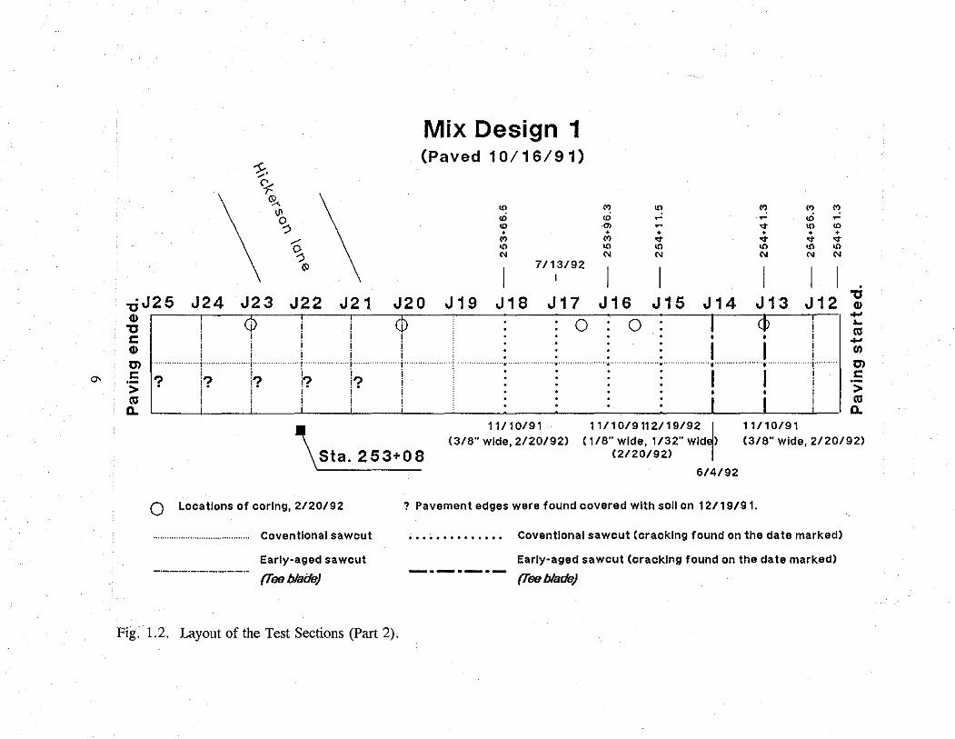
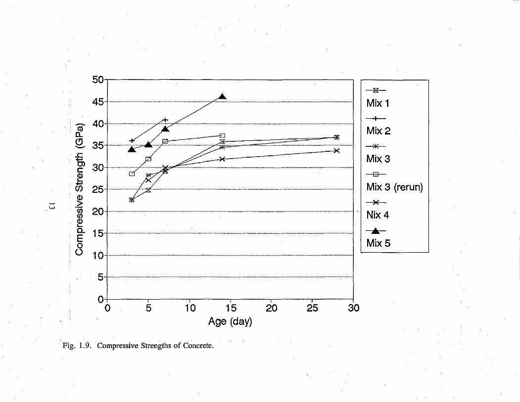
Compression tests were performed for each mix design at concrete ages of 3, 5,

7, 14 and 28 days. Fig. 1.9 shows the increase in the compressive strength with the

concrete age. Obviously, the specimen of Mix Design 5 (with crushed limestone as the

coarse aggregate) had higher tensile and compressive strengths at these ages than Mix

Designs 1, 3 and 4 (all with siliceous river gravel as the coarse aggregate) at these

3

concrete ages. Mix Design 2 was different from Mix Design 5 by the replacement of

50% of 1.5-inch (38 mm) limestone by 0. 75-inch (19 mm) siliceous river gravel (Table

1.1). Although the compressive strength of Mix Design 2 was higher (Fig. 1.9) than

that of Mix 5, it did not show a higher tensile strength at the age of 7 days (Table 1.2).

Mix Designs 3 and 4 used the same fine aggregate and the same intermediate aggregate,

but the coarse aggregate in Mix 3 was nominally 1.5 inches (38 mm) while Mix Design

4 was nominally 0.75 inch (19 mm). As a result, Mix 3 had higher compressive and

tensile strengths than Mix 4. On the other side, though Mix Design 1 had a larger

coarse aggregate than Mix Design 4, these two mix designs had similar tensile and

compressive strengths at the age of 7 days. It may be interesting to note that the

compressive strength of Mix 4 was higher than that of Mix 1 at the age of 5 days, but

lower after the age was older than 7 days.

Table 1.2. Average Flexural Strength at the Age of Seven Days.

Mix Design Average Flexural Strength Standard Deviation

1 662 psi (4.56 MPa) 34 psi (0.23 MPa) .

2 805 psi (5.55 MPa) 50 psi (0.34 MPa)

3 693 psi (4.78 MPa) 27 psi (0.19 MPa)

4 662 psi (4.56 MPa) 26 psi (0.18 MPa)

5 841 psi (5.80 MPa) 46 psi (0.32 MPa)

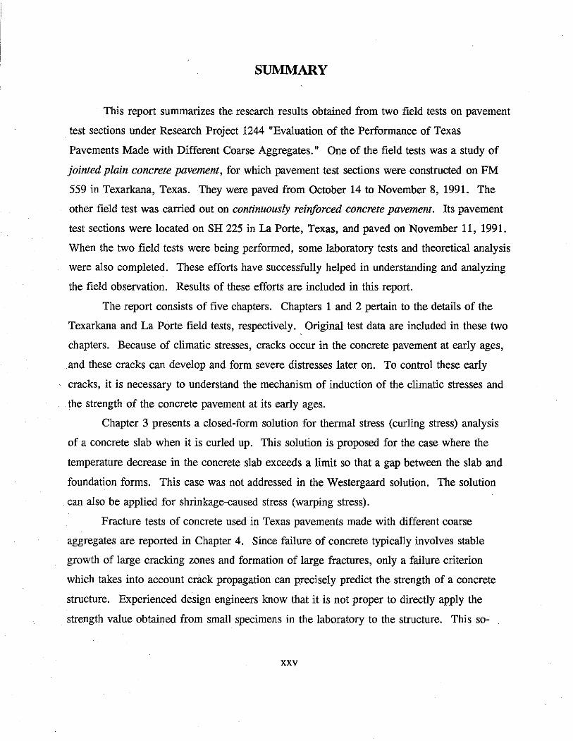
The pavement shown in Fig. 1.1 is the test section paved on October 14, 1991

with the concrete of Mix Design 3. Fig. 1.2 shows another segment of paving

completed in one day, which was paved with Mix Design 1 on October 16, 1991.

Three segments paved on October 18, October 26, and November 6, 1991, all used Mix

Design 5 as shown in Figs. 1.3 to 1.6 respectively. The test section of Mix Design 2

was paved on November 8, 1991, and its layout is shown in Fig. 1.7. The six test

4

J10 J9 JS ,, I I CJ) ,, • • • c I I I CJ)

D'I ....................... ........ ........... J .... ··········· i

c I I > • • • Ill I I I D. t 6/4/92 6/4/92 6/4/92

Jl 1 as counted by TxDOT

O Locations of coring, 2/20/92

Coventlonal sawcut

Early-aged sawcut

(Tee blade)

Mix Design 3 (PaVed 10/ 14/91)

J7 JS

<b • • I I

.... •. .........................

I I • • I I

6/4/92 6/4/92

0

"' ~ "' • "' "' N

JS

' I

·······'···· I ' I . I

J4

0 I • I

........... --~ ...

I • I

6/4/92

10/ 16/91

(1/4" wide, 2/20/92)

----·------------------·---

"' "' .,; ~

0 ~

• • "' "' "' "' N N

I I J3 J2 J1 ,,

CJ) -... Ill -f/l D'I c > Ill D.

6/4/92 614192

Coventlonal sawcut (cracking found on the date marked)

Early-aged sawcut (cracking found on the date marked)

(Tee blade)

Fig. 1.1. Layout of the Test Sections (Part 1).

Mix Design 1 (Paved 10/16/91)

"' "' <D .,; "! ~ "' ~ ~ .,;

<D "' ~ ... "' <D

• • • • • • "' "' ... ... ... ... "' "' "' "' "' "' "' "' N N N N

7/13/92

,;J25 J24 J23 J22 J21. J20 J19 J18 J17 J16 J15 J14 J13 J12 -g ~ ,-----~~ri ~~-x~~-ri~~-.i~~-:r~~~~~~~~~~~o=-~~o=-~~~--j,--~---,i:-~~,i ~,

C i I i j I . • • • j G> i i i i i • • I I i

1• i i i i i m ···········i·· ..... ············i ···················i·· ···i···· ········ ····t ... · ····' · ··················•···· .................... . ...... ·· ..................... ·················•··········· ········•··· ··· ···· ······i ... ..

.: ?. i? i? :,'.?. i? i I I i,. > ! • l · i. i i cu ! ! ! i i c..

-... m -f/I Cl c > m c..

\Sta. 253+08

11110/91 (3/6" wide, 2/20/92)

11/10/9112/19/92 ~ 11/10/91 C 116" wide, 1/32" wld ) (3/6" wide, 2/20/92)

O Locations of coring, 2120/92

Coventlonal sawcut

Early-aged sawcut

(Teo blade)


(2120/92)

6/4/92

? Pavement edges were found covered with soil on 12119/91.



(Teo blade)

"' "' • ~

"' N

J32

"' ... •

<O N

J31

I ............. ... ................... .

I

2/20/92

11/10/91

Mix Design 5 (Paved 10/ 18/91)

J30

; ;

....... ~ ...

J29

!

"' ~ • N

"' N

J28 J27

I ; ......... ) .... . .. . ....• . i

I '

11/10/91

(5/ 16" wide, 2/20/92)

(3/8" wide, 2/20/92)

? Pavement edges were found covered with soil on 12/ 19/91.

J26 J25.; GI

! ...... !.. .

; !? i •

.... ... (II .... (/)

m c > (II

a.

Coventlonal sawcut Conventional sawcut (cracking found If any)

Early-aged sawcut

(Sfmight blade) -··-··-··-



(Sfmight blade)

CX> .,; N +

0

"' N

J40


CX>

m "' + + 0 0

"' "' N N

I I J39 J38 J37

r ! I

I

! I

7/13/92 6/4/92

Crack found 11/10/91 (1/4" Wide, 2/20/92)

J36 J35 I

1 I ! .. .

I i !? i

' 6/4/92

J34 J33 ' !

i

······l ......... J. ... i

co "' +

"' N

J32

! I

I

11/10/91

____ .. " ___________ _

? Pavement edges were found covered with soil on 12119/91.

Coventlonal sawcut

Early-aged sawcut

(Straight blade)

..............


Conventional sawcut (cracking found If any)


(Straight blade)

,, Cl> ,, c Cl> Cl c ·-> m a.

N ... • Cl) ... N

J13 J12 J11 J10

Cl) ... l'i 0 • "' ... N

J9

Mix Design 5 (Payed 10/26/91)

"' ~ • O> ... N

JS J7 J6

Cl)

.; N N • •

0 0

"' "' N N

I I JS J4 J3 J2 J 1 'g

~-.,~~~~,~~~~,~~~,--~~-T1.~~~.,.-~~_,-~~~r1.~()~--,-rtl~-()~-r1.~~~r1.~~~r,,~~~,~~t'.

l l I l ! t I I ! ~ i m , , , . , , , ! 1 i , ! , en I r I r I ! ! ! ! ! ! ! !

·-·-·i-·-·-·-·-·-t-·-·-·-·-·+·-·-·-·-·-i-·-·-·-·---+·-· ·-·-·-+-·-·-·-·-·-t·-·-·-·-·-·+-·-·-·-·-·-J.-·-·0-:-·+·-·-·-·-·-1---·-·-·-·+·-·-·-·-·-•-·-·- m i i i i i ! i ! i ! j ! i c Ii

1!

1j !

1 !1

I I I I l I I I •-j i j i i ! i ! >

i i i i i ... ,! ,! ,! ! ! ,! ,! ,! m '----''~~~J'~~~J'~~~4'~~~~··~~''---1-~~~-'--~~-'-~~~J__~~-'-~~~J.-~~-'-~~--''----'D.

r Not counted as J 14

Crack found 11/10/91 (3/ 16" wide, 2/20/92)

() Locations of coring, 2/20/92

Early-aged sawcut -------(Tee Blade)

Early-aged sawcut (cracking found If any>

(TeeB/ade)


-0

'ti Cl> 'ti c Cl> IJ') c ·-> cg

D..

"': ~

"' + <O ... N

J25 i i

J24 J23

' '


Crack foud 7/13/92

Lopatlorl of••-•-·••• 17 ts Fliehtiiond •

,.., N ., ...

+ + <O <O ... ... N N

I 1-o J22 J21 J20 J19 J18 J17 J16 J15 J14 ! ...

i i i cg i l j • i +'

----~-----

i ----- J J ......... ! ..... -+--_-___ J. __ :_-___ -----r~--1;:------j~----~---··-··-··L··-··-··-··-··l··-··-··-··-·.J··-··-··-··-··l··-··-- ~ I ................... j ! ! ! C I i i i

' ' I I

6/4/92 6/4/92

Coventlonal sawcut

Early-aged sawcut

(Tee Blade)

Early-aged sawcut

(Straight blade)

i j I I I •-i i i i i > i i i i i cg

D.. 11/26/91 6/4/92 6/4/92

( 1/8" wide, 2/20/92)

Conventional sawcut (cracking If any)


(Tee Blade)

Early-aged sawcut (cracking found If any)

{Straight blade)


--

1J (])

ll. ll. 0 -rn lJl c > (ll

0..

m 0 . "' "' "'


- "' M ct) M a)...:

<:> ~ '!? ~~ '<t '° lO U)<O '<t '<t '<t '<t 'd" N N N N N

7/13/92 1J

J20 P,15 ? ? J10 JS J1 ~ : : 0 0 o • , o , ; j f f f I I I f I /.) ioi Cl J _______ : ____ ;_ __ ;_ __ ;_ __ : __ _; __ ~ _____ J ___ L __ L __ L __ L __ J ___ J __ J __ J __ ::t?._[ __ _[__ c • · • . J I f I I I I I I t I I >

,! i i. l'tl '--"--~--~----~------~----~--~--.L----11--__,_ __ _,_ __ ..____,,____,_ __ _,_ __ .._____,,___,_ __ ..L.....J 0..

6/4/92 6/4/92 ~I/ 6/4/92

11/26/91

C 1/8" wide, 2/20/92)

11/26/91

C 1/8" wide, 2/20/92)

11/26/91

C 118" wide, 2/20/92)

2/20/92

( 1/8" wide, 2/20/92)


Coventlonal sawcut

Early-aged sawcut

(Tee blade)

Fig. 1. 7. · Layout of the Test Sections (Part 7).



(Tee blade)

-p % ,,..

\ \

,. , J 12 ....... \·_ ............ ·

..... ..... \ \ .. J 11 \/ ,. ,,.,. \ "' ~


"' "' " .;

----.-~------~--·-------'-------- --~'

"' ~ ".'.>\{>

0 ".'.> 11/10/9

\ \ ..... ....-· J10 "' • N " • N

r-. • N

.; "' 0 0 • •

(') "' ~

0 0-

..... ).< ..... .. /,,,. \ J9

\ ,, 7/13/92 ),,..-··"' I

..... ,.,.. ,,-·· )

" " N N " N

J2

" " N N

I I J1 ; JS J6 JS J4 J3

'--.------------~----0 0 iJ7 '

J ..... ... J ' ...... L ' ......... L ' ' .......... L .... J .. I ' • ' ' ' i I i j

I I I I 11126/91 2120/91 11/10/91 6/4/92

( 1 /6" wide, 2120/92) (< 1/ 16", 2/20/92) (<1/16")

i i I

.J ... ! I ! !

F.M. 559

O Locations of coring, 2/20/92

Coventlonal sawcut

Early-aged sawcut

(Tee blade)

Early-aged sawcut

(Straight Blade) -··-··-··-


Conventional sawcut (cracking found If any)


(Tee blade)


(Straight blade)

~

45 ················--··················································· ··········································································································· Mix 1

t c:

~ 25 ····························· ·······················································································································································

~

Mix2

Mix3 D

Mix 3 (rerun) ---..)(--

"(i) (/)

20 ····································································································································································. Nix4 ~ 0. E 0 0

15 ···············································································································································································

10 ··································································································································································

5 ·····················································································································································

01-1-~~~~~~~~~~~~~~~~~~~---<

0 5 10 15 20 25 30 Age (day)

Fig. 1.9. Compressive Strengths of Concrete.

-A

Mix5

section segments mentioned were all paved from south to north. Another test section

(Fig. 1.8) was paved from south to north and then turned to northeast. This section

used Mix Design 4 and was paved on October 22, 1991, using a vibrating screen. It

was noted by the contractor that the concrete was very easy to place using this mix

design as were all the mix designs using the intermediate aggregate. This was

evidenced further by the lack of "honey combing" in core samples obtained several

months after the concrete was placed.

Four different curing methods were employed in this experimental section. These

curing methods are as follows:

(i) Membrane curing compound, Item 360.2 (13), which is called the

standard curing method;

(ii) Membrane curing compound, Item 360.2 (13), using Procrete - a

proprietary product;

(iii) Cotton mat curing, Item 360.2 (15), plus membrane curing, Item 360.2

(13), called "Cotton Mat";

(iv) Polyethylene film curing, Item 360.2 (12), plus membrane curing, Item

360.2 (13), called "Polyethylene" for brevity.

1.3. JOINT SA WCUTTING

As described previously, two sawcut techniques were used for longitudinal and

transverse joints: conventional sawcutting and early-aged sawcutting. The early-aged

sawcut technique uses a light and portable sawcut machine that allows the pavement to

be cut earlier than by using the conventional sawcut technique, differing from the

conventional sawcut method, which uses water to cool the blade during cutting

operations.

The spacing of the transverse joints in this experimental pavement was 15 feet

(4.57 m). The notch cut by the early-aged sawcut method was approximately 1 inch (25

mm) deep. The conventional method was used to cut the pavement D/4 which was

approximately 3 inches (76.2 mm) deep. The sawcut methods used at each joint are

noted in the layout of each test section (Figs. 1.1 to 1.8). Two different types of

14

diamond blades were used with the early-aged cutting method. One was T-shaped while

the other was a straight blade.

Early-aged sawcut operations generally started 4.5 to 5.5 hours after placement of

the concrete. When the weather was cold and humid, dry sawcut was delayed until the

pavement was solid enough to walk on. In some instances, this delay was extensive.

For example, in the test section where Mix Design 3 was used, the paving started at

9:00 a.m., and it was not sawcut until midnight. No apparent ravelling happened along

the notches sawcut by the early-aged sawcut technique.

1.4. WEATHER INFORMATION

Weather information was obtained from the weather station at the Texarkana

airport, located in Texarkana, Arkansas. The highest and lowest temperatures from

October 13 to November 11, 1991 are shown in Fig. 1.10. Daily average temperatures

during this period are given in Fig. 1.11. A portable weather station, Campbell

Scientific 012, was placed near the test sections and obtained ambient temperature and

relative humidity from November 7 to 10. Fig. 1.12 shows these data.

1.5 MEASUREMENT OF COMPRESSIVE STRENGTHS OF CONCRETE SPECIMENS PREPARED IN THE FIELD

Cylindrical specimens and beam specimens were prepared and cured in the field

while each mix design was placed. The cylindrical specimens were 6-inch (152 mm) in

diameter and 12-inch (305 mm) in height. Data from the compression tests are shown

in Table 1. 3.

15

30

0 .._.. (/) (I) .._ ii'

::J -m .._ 20 (I) 0.. E (I) I-"ti) Q)

10

~ -' 'U - c

"' cu +-' (/)

0 Q) .c 0)

I >.

·cu D -10

12 16 20 24 28 1 5 9

October 1991 I November 1991

Date

Fig. 1.10. Daily Highest and Lowest Temperatures.

--------- -~---~--------

0 ._.... Q) ..... :::l al 20 ..... Q) 0.. E Q)

f-Q) - l'.J)

-.) «l ..... 10 Q)

~ >. . «l 0

12 16 20 24 28 1 5 9

October 1991 November 1991

Date

Fig. L 11. Daily Average Temperatures.

-00

, ... __ , ' . : \ , '

; \ \ I I

\ ,' i 15 \._.,,/ \

" " ' ' \ / \

v ' \

" 10 '

5

' \ \ \ ' \

\ \ \

' / \ ' . , ' . .

I \

! \ : \ , ' . . , ' ' . , '

Nov. 10

: ·' : J \ !

\ : \ - r

' \ \ : ...... ,, \ '- \ :

100

90

80

70

60

50

40

'\ \ I \ : / I ' f ································································· .............. \............ r··········· -· ···········\· ... ··························r· .. ····· ····-······ ············- ............. ,-·······-;-······ 30

' _. \ I ._...,.,/

............ / ' :' \ :

!Nov. a j .... , : ' : ' " -~,

20

-5+-~~~~~~~~.i-~~~~~~~--1~~~~~~~~-+~~~--1-10

0 24 48 72 12 36 60 84

Time (hour)

\----- Temperature - Relative Hunidity

Fig. 1.12. Temperature and Relative Humidity Records by the Weather Station.

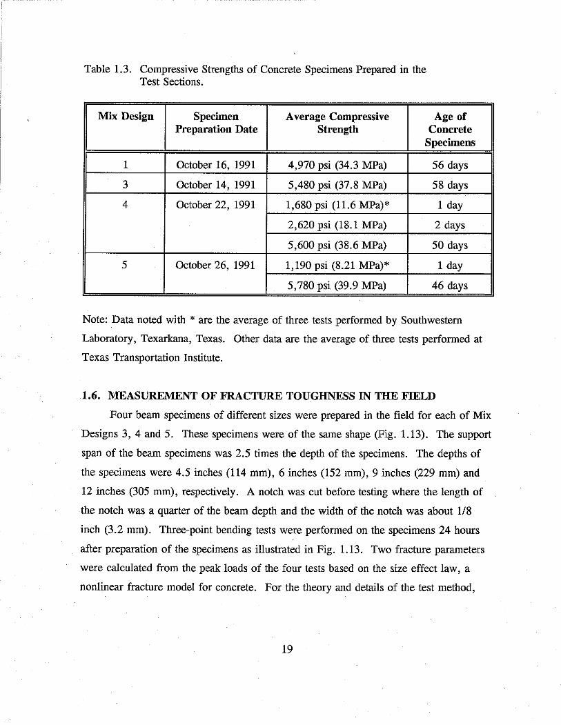
Table 1.3. Compressive Strengths of Concrete Specimens Prepared in the Test Sections.

Mix Design Specimen Average Compressive Preparation Date Strength

Age of Concrete

Specimens

1 October 16, 1991 4,970 psi (34.3 MPa) 56 days

3 October 14, 1991 5,480 psi (37.8 MPa) 58 days

4 October 22, 1991 1,680 psi (11.6 MPa)* 1 day

2,620 psi (18.1 MPa) 2 days

5,600 psi (38.6 MPa) 50 days

5 October 26, 1991 1, 190 psi (8.21 MPa)* 1 day

5,780 psi (39.9 MPa) 46 days

Note: Data noted with * are the average of three tests performed by Southwestern

Laboratory, Texarkana, Texas. Other data are the average of three tests performed at

Texas Transportation Institute.

1.6. MEASUREMENT OF FRACTURE TOUGHNESS IN THE FIELD

Four beam specimens of different sizes were prepared in the field for each of Mix

Designs 3, 4 and 5. These specimens were of the same shape (Fig. 1.13). The support

span of the beam specimens was 2.5 times the depth of the specimens. The depths of

the specimens were 4.5 inches (114 mm}, 6 inches (152 mm), 9 inches (229 mm) and

12 inches (305 mm}, respectively. A notch was cut before testing where the length of

the notch was a quarter of the beam depth and the width of the notch was about 1/8

inch (3.2 mm). Three-point bending tests were performed on the specimens 24 hours

after preparation of the specimens as illustrated in Fig. 1.13. Two fracture parameters

were calculated from the peak loads of the four tests based on the size effect law, a

nonlinear fracture model for concrete. For the theory and details of the test method,

19

Fig. 1.13. Geometry of the Beam Specimen.

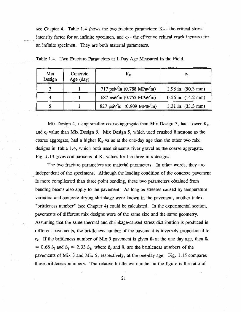
see Chapter 4. Table 1.4 shows the two fracture parameters: Kif - the critical stress

intensity factor for an infinite specimen, and c, - the effective critical crack increase for

an infinite specimen. They are both material parameters.

Table 1.4. Two Fracture Parameters at 1-Day Age Measured in the Field.

I Mix

I Concrete

I Kif I c,

I Design Age (day)

3 1 717 psi:v'in (0.788 MPaVm) 1.98 in. (50.3 mm)



Mix Design 4, using smaller coarse aggregate than Mix Design 3, had Lower Kif

and c, value than Mix Design 3. Mix Design 5, which used crushed limestone as the

coarse aggregate, had a higher Kif value at the one-day age than the other two mix

designs in Table 1.4, which both used siliceous river gravel as the coarse aggregate.

Fig. 1.14 gives comparisons of Kif values for the three mix designs.

The two fracture parameters are material parameters. In other words, they are

independent of the specimens. Although the loading condition of the concrete pavement

is more complicated than three-point bending, these two parameters obtained from

bending beams also apply to the pavement. As long as stresses caused by temperature

variation and concrete drying shrinkage were known in the pavement, another index

"brittleness number" (see Chapter 4) could be calculated. In the experimental section,

pavements of different mix designs were of the same size and the same geometry.

Assuming that the same thermal and shrinkage-caused stress distribution is produced in

different pavements, the brittleness number of the pavement is inversely proportional to

c,. If the brittleness number of Mix 5 pavement is given Jl5 at the one-day age, then Jl3

= 0.66 Jl5 and Jl4 = 2.33 Jl5, where Jl3 and Jl4 are the brittleness numbers of the

pavements of Mix 3 and Mix 5, respectively, at the one-day age. Fig. 1.15 compares

these brittleness numbers. The relative brittleness number in the figure is the ratio of

21

N N

K If (MPa• ni'2 )

1

Mix Design #3 Mix Design #4

Fig. 1.14. Fracture Toughness of Concrete Measured at One-Day Age.

Mix Design #5

Relative Brittleness Number 2.5 .-~~~~~~~~~~~~~~~~~~~~~~~~~~~~~~~-

2

1.5

N w 1

0.5

Mix Design 3 Mix Design 4 Mix Design 5

Fig. 1.15. Brittleness Number for Pavements of Different Mix Designs at One-Day Age.

the brittleness number of the specific pavement to the brittleness number of the

pavement of Mix 5. It will be seen later in this report that the larger the brittleness

number at the one-edge age, the more sawcuts cracked at early ages. (The percentage

of cracked sawcuts is shown in Fig. 1.26 of Section 1.9.)

1.7. MEASUREMENT OF PAVEMENT TEMPERATURE AND RELATIVE HUMIDITY

Temperature and relative humidity are two important variables in their effect on

concrete. Changes in either of these conditions can induce stresses in the pavement as

well as affect the rate of the strength gain of the concrete. The influence of these

parameters is very apparent during the early ages of the concrete. Both temperature and

relative humidity in the test sections were measured with three different digital systems.

One system, a product of Vaisala, measures both temperature and humidity in the

concrete, where the sensor works on a capacitance basis. It monitors the change in

capacitance of a thin polymer film as it absorbs water vapor. Another sensor,

manufactured by General Eastern, measures the change in electric resistance of a bulk

polymer sensor with the moisture that the sensor absorbs. The third digital system used

was a product of Omega.

To apply these instruments, a PVC tube was inserted in the pavement surface.

The sealed tube was placed while the concrete was fresh so that the concrete exposed

inside the tube was protected from the outside atmosphere (Fig. 1.16). When the

temperature and relative humidity were measured, the probe of

the measuring system was inserted in the PVC tube with a rubber "O" ring to seal the

small space between the sensor unit and the wall of the PVC tube. After the

measurement, the probe was removed from the PVC tube, and a PVC cap was screwed

on the top end of the tube to prevent air exchange between the space inside the tube and

the atmosphere.

For comparison of different curing methods, temperature and relative humidity

data for the test section using Mix Design 3, which was placed on October 14, 1991 are

shown in Figs. 1.17 and 1.18. Data were collected at different times as shown in the

24

Digital Display

Seal

/General Eastern Meter

/PVC Tube

Sensor

............ ..... ..... .. ·-·· .. .... . ..... ···-::::::.:::.:::·:·:::::::::::::::.:.:::.:-··· .... . ·.·.·.·.·.·.·-:-:-: :-:.:.:-:-:..-.·.-:: :-. :·::::·:::::::::::::::::

:·:: : i ::;:::::::::: ii1i1i::1 ::;:::i::;:::;;:;: ! :::-::.,...,.,~ •.• ~~:·i :·i :·~ :·i:·i:~:::::::::.::-.:.: ::::· ·:: ::: ::::::-: ::·::::-:::::::::::::::::: i:k·:.

:::::::::'::::::::::::::::::::::::::::::::::::::::= = .. 99Hsr~J~_::i:)-~¥~m~mt, :::

Fig. 1.16. Sketch of the Setup for Relative Humidity Measurement in Concrete.

25

Temperature (C) 30 r-~~~~~~~~~~~~~~~~~~~~~~~~

25

20

15

10

5

10/14/91 (10:00 p.m.)

10/16/91 (11 :oo p.m.)

10/22/91 (7:00 p.m.)

~ Cotton Mat m Polyethylene rssl Standard

Fig. I. 17. Temperatures in Concrete (Mix Design 3, Paved on October 14, 1991).

11/26/91 (2:00 p.m.)

R.H. (%) 120 .--~~~~~~~~~--.,.~~~~--.,.~~~~~~~--,

100

80

60

N -i 40

20

10/14/91 (10:00 p.m.)

10/16/91 (11 :oo p.m.)

10/22/91 (7:00 p.m.) .

[Zi Cotton Mat IB Polyethylene ~ Standard

Fig. 1.18. Relative Humidity in Concrete (Mix Design 3, Paved on October 14, 1991).

11/26/91 (2:00 p.m.)

figures. It is speculated that the pavement covered by the cotton mat obstructed solar

radiation and resulted in a lower pavement temperature as compared with the pavement

cured with the standard method. The pavement section covered with polyethylene film

was subjected to a "greenhouse" effect, which made the temperature in the pavement

higher than in the pavement cured with the standard curing method. On the other hand,

the relative humidity in the pavement cured with the cotton mat method and the

polyethylene method was higher than in the pavement cured by the standard curing

method. This was because the cotton mat and the polyethylene film isolated the

pavement top surface from the atmosphere and kept the moisture in the pavement from

evaporating. The differences between the temperatures and relative humidities in the

pavements cured with the three different methods decreased after approximately 30

days. The cotton mat and polyethylene film remained in place on the pavements for

seven days after pavement construction. The differences in temperature and relative

humidity caused by different curing methods in the test section of Mix Design 2, placed

on November 8, 1991 (Figs. 1.19 and 1.20), showed similar trends observed in the test

section of Mix Design 3.

In the test section of Mix Design 4, a different trend in temperature is observed in

Fig. 1.21. In the first two days, the temperature in the pavement covered by cotton mat

was the highest of all the curing test sections. On the third day, temperatures in the

pavement sections covered by cotton mat and polyethylene film were lower than

pavement sections cured with the standard method. This may have been caused by an

increase in the ambient temperature which occurred from October 22 to 25 (Fig. 1.10).

In the previous two cases (Mix Designs 2 and 3), ambient temperatures tended to

decrease from those which occurred during the paving with these mixes. The pavement

cured with the standard method may have absorbed more solar radiation thereby

affecting the temperatures in the pavement. There was no apparent difference in the

relative humidity with respect to the curing method (Fig. 1.22). However, by the third

day, the relative humidity in the test sections covered by either cotton mat or

polyethylene film was higher than the relative humidity in the test sections with the

standard curing method. As far as the proprietary-product method, higher pavement

28

Temperature (C) 14 ~~~~~~~~~~~~~~~~~~~~~~~~~~~~~~~~-,

12

10

8

6

4

2

0 11/8/91

(4:30 p.m.) 11/9/91

(10:00 a.m.)

~ Cotton Mat Ill Polyethylene [J Standard

Fig. 1.19. Temperatures in Concrete (Mix Design 2, Paved on November 8, 1991).

R.H.(%) 120

100

80

60

w 0 40

20

0 11/8/91

(4:30 p.m.)

~ Cotton Mat

11/9/91 (1 o:oo a.m.)

¥&% Polyethylene I••• I Standard

Fig. J.20. Relative Humidity in Concrete (Mix Design 2, Paved on November 8, 1991).

--------------~·"~~ .-----·--------

Temperature (C) 35

30

25

20

15

10

5

0

••••••

10/22/91 (6:00 p.m.)

10/23/91 (6:00 p.m.)

10/24/91 (6:00 p.m.)

10/25/91 (3:30 p.m.)

~ Cotton Mat • Polyethylene ~ Standard [J Proprietary product

Fig. 1.21. Temperatures in Concrete (Mix Design 4, Paved on October 22, 1991).

R.H. (%) 120

100

80

60

40

20

0 10/22/91 (6:00 p.m.)

10/23/91 (6:00 p.m.)

10/24/91 (6:00 p.m.) _

10/25/91 (3:30 p.m.)

~ Cotton Mat • Polyethylene ~ Standard !I] Proprietary product

Fig: 1.22. Relative Humidity in Concrete (Mix Design 4, Paved-on October 22, 1991).

temperature andJower relative humidity. occurred on. the third daythanthose_inthe

pavement sections cured with the standard method.

The test section consisting of Mix Design 5 was placed on October 26, 1991,

after which construction delays occurred due to rainfall which continued through

November 6. Another test section of Mix Design 5 was placed on November 6, 1991.

The test section of Mix Design 1 was placed on October 16, 1991.

1.8. MEASUREMENT OF PULSE VELOCITY OF PAVEMENT

The basic idea behind the pulse velocity method is: Given the velocity of a

longitudinal wave through a medium and the density and Poisson's ratio of the medium,

then the dynamic modulus of elasticity of the medium can be computed. Furthermore,

knowing the modulus of elasticity, other mechanical properties can be estimated from

empirical correlation with the dynamic modulus of elasticity.

Pulse velocity measurements in test sections of Mix Designs 2, 3, 4 and 5 were

performed. Previous research had indicated that temperature and moisture conditions of

the concrete had insignificant effects on the pulse velocity readings.

The V-Meter, a portable ultrasonic testing unit, was provided by the Federal

Highway Administration (FHW A) and used in the test sections to measure the pulse

velocity. The V-Meter uses transducers, each for transmitting and receiving the

ultrasonic pulse. The pulse travel time is displayed in three numerical digits ranging

from 0.1 to 999 micro-seconds. In the test sections, the two transducers were placed on

the pavement top surface, 12 inches (305 mm) apart from each other. Grease was used

to improve the contact between the transducer end surface and the pavement surface.

The pulse velocity was simply obtained by dividing the distance between the two

transducers, 12 inches (305 mm), by the recorded pulse traveling time, and then

multiplied by a factor 1. 05. The factor 1. 05 was a compensation for the pulse

travelling distance since the pulse path was not along a straight line (Fig. 1.23). This

technique was also applied in the field test in La Porte (Section 2. 6).

33

TX

..... : .· . : . . · . :

• •

l TA

. . • • • • • . " .

•••• : . -

----------- -------- ------,rl--

Fig. 1.23. Pulse Traveling Path in the Pulse Velocity Measurement.

Measurements show that the pulse velocity increased rapidly in the first days after

concrete was paved. For example, Fig. 1.24 shows changes in the pulse velocity in the

test section of Mix Design 5 paved on October 26, 1991. The origin of the time scale

in the figure is the time of pouring for the part where measurements were performed,

that is, 10:00 a.m., October 26. It is apparent that the pulse velocity increased even

more in the first several hours than at later ages, which reflects the fact that the strength

of concrete increases at a greater rate in the early ages. The pulse velocity was

correlated with early-aged sawcutting operations. These values ranged from 4.38 x HY'

inches/sec or 3650 feet/sec (1110 m/sec) in the concrete cured with the polyethylene

method, and 5.5 x 104 inches/sec or 4580 feet/sec (1400 m/sec) in the concrete cured

with the proprietary product. No apparent ravelling occurred along the dry sawcuts.

1.9. ANALYSIS OF SPECIMENS CORED FROM THE PAVEMENT

Specimens of four inches (102 mm) in diameter were cored from pavement of

different mix design test sections on February 20, 1992. The coring locations are all

noted in Figs. 1.1 to 1.8. These specimens were observed and tested for the following

engineering properties and features: (a) Honeycombing, (b) Compressive Strength, (c)

Elastic Modulus, and (d) Split Tensile Strength.

To explain honeycombing, an index has been developed called as "level of

honeycombing." Level of honeycombing is defined in terms of size and spacing of air

pockets in concrete. The smallest air pocket considered is an elongation of 1/8 inch

(3.2 mm). The different severity levels of honeycombing, which are somewhat

subjective in natures are given in Table 1.5.

Measuring elongation and spacing of air pockets can be done by linear traversing,

but specifying the common spacing is difficult as air pockets are scattered randomly in

the concrete body. In most of the cored specimens, the maximum elongation of air

pockets is 1/2 inch (12. 7 mm). For these specimens, severity of honeycombing can be

described in terms of spacing of the air pockets as follows:

35

w 0\

'U' QI

-!!!. a ._, a ·-(.I 0 -QI > QI Ill -0

i:i..

6000

5000

4000

3000

2000

1000

0+-.--.--.--.--.-.-.--r--r--r-,--,---;;-----r--.,----.j 0 100 200 300 400 500 600 700 800

Time (hours)

-polyethylene -+-

cotton -proprietary product -a-

standard

Fig. 1.24. Pulse Velocities in the Test Section of Mix Design 5 (Paved on October 26, 1991).

Table 1.5. Criteria for Level of Honeycombing.

Level of Honeycombing Severity

A low (small air pockets)

B moderate (small air pockets)

c high (small air pockets)

D very high (small air pockets)

I very high (large air pockets)

Level of Honeycombing A - indicates presence of air pockets with a spacing of 2

inches (50.8 mm) or more which is consistently distributed.

Level of Honeycombing B - indicates presence of air pockets with a spacing of

1/2 - 1 inch (12. 7 - 25 .4 mm) which is sparsely distributed.

Level of Honeycombing C - indicates presence of air pockets with a spacing of

1/2 inch (12. 7 mm) which is less densely distributed than level D.

Level of Honeycombing D - indicates presence of air pockets very closely

distributed with a consistent spacing as small as 114 inch (6.4 mm).

In the cored specimens of Mix Design 1, elongation of air pockets is very large.

The maximum elongation is near 1 inch (25.4 mm), and spacing is as large as 1 - 2

inches (25.4 - 50.8 mm). It may be because of lack of intermediate aggregates. A

description of this honeycombing case is provided below:

Level of Honeycombing I - indicates presence of large air pockets up to 1 inch

(25 mm) long, with a spacing of 1 - 2 inches (25.4 - 50.8 mm), which is sparsely

distributed. In terms of percentage of air pockets over the lateral surface of the cored

specimen, severity of Level 1 may be equivalent to Level C or Level D.

Level of honeycombing of cored specimens taken from each mix design is listed

in Table 1.6.

One cored specimen of each mix design was tested for the compression strength

on July 2, 1992. The 13-inch (330 mm) long core was cut at both ends with a diamond

saw to make the specimen 12 inches (305 mm) long. The specimen was capped before

37

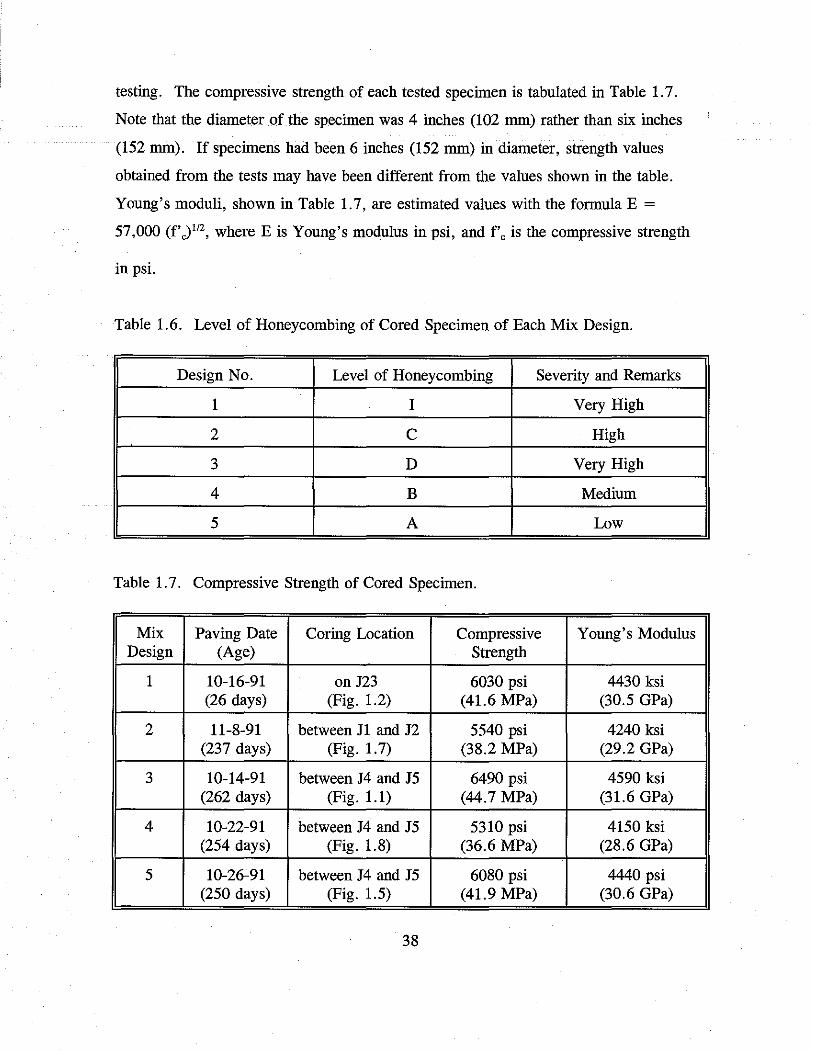
testing. The compressive strength of each tested specimen is tabulated in Table 1. 7.

Note that the diameter of the specimen was 4 inches (102 mm) rather than six inches

(152 mm). If specimens had been 6 inches (152 mm) in diameter, strength values

obtained from the tests may have been different from the values shown in the table.

Young's moduli, shown in Table 1.7, are estimated values with the formula E =

57,000 (f'J112, where Eis Young's modulus in psi, and f'c is the compressive strength

in psi.

Table 1.6. Level of Honeycombing of Cored Specimen of Each Mix Design.

Design No. Level of Honeycombing Severity and Remarks

1 I Very High

2 c High

3 D Very High

4 B Medium

5 A Low

Table 1. 7. Compressive Strength of Cored Specimen.

Mix Paving Date Coring Location Compressive Young's Modulus Design (Age) Strength

1 10-16-91 on J23 6030 psi 4430 ksi (26 days) (Fig. 1.2) (41.6 MPa) (30.5 GPa)

2 11-8-91 between J1 and J2 5540 psi 4240 ksi (237 days) (Fig. 1.7) (38.2 MPa) (29.2 GPa)



5 10-26-91 between J4 and J5 6080 psi 4440 psi (250 days) (Fig. 1.5) (41.9 MPa) (30.6 GPa)

38

Although Mix 2 showed higher compressive strengths than the other mixes at ages

of three days and five days in the lab tests (Fig. 1.9), the cored specimen of Mix 2 had

a lower compressive strength than Mixes 1, 3 and 5 due to the level of honeycombing

that was evident in this mix.

For Mixes 1, 2, 3, and 5, split tension tests were performed on July 8, 1992.

The cored specimens were cut with a diamond saw into three or four 3-inch (76 mm)

thick cylindrical specimens. The split tensile strengths of these specimens are shown in

Table 1.8.

Table 1.8. Split Tensile Strength of Cored Specimen.

Mix Paving Coring Location of Split Tension Split Tensile Date Location Specimen from Top Strength

Surface of Pavement

1 10-16-91 between 0-3" (0-76.2 mm) 595 psi (4.10 MPa) J16 and

3-6" (76.2-152 mm) 613 psi (4.23 MPa) J17 6-9" (152-229 mm) 681 psi (4.70 MPa)

9-12" (229-305 mm) 725 psi (5.00 MPa)

2 10-22-91 on J3 1.5-4.5" (38-114 mm) 613 psi (4.23 MPa)

4.5-7.5" (114-191 mm) 706 psi (4.87 MPa)

7.5-10.5" (191-267 mm) 722 psi (4.98 MPa)

3 10-14-91 on J6 1.5-4.5" (38-114 mm) 738 psi (5.09 MPa)

4.5-7.5" (114-191 mm) 780 psi (5.38 MPa)

7.5-10.5" (191-267 mm) 840 psi (5. 79 MPa)

5 10-26-91 between 0-3" (0-76.2 mm) 645 psi (4.45 MPa) J5 and J6

3-6" (76.2-152 mm) 730 psi (5.03 MPa)

6-9" (152-229 mm) 803 psi (5.54 MPa)

Data shown in Table 1. 8 indicate that the tensile strength of concrete increases

with the depth in the pavement. These data are plotted in Fig. 1. 25. The distance of

39

* D

* Mix 1 5- ............................................... '+.' .................... l:J ..................................................................... +····················~··················

+ + C? a. :2: -Cf) ..c

x D

* Mix3

x + x 4-············· ....................... ................. ............. ·················································· ··························

Mix2

..... C> c: D

~ ..... Cf)

3-··································································· ................................................................................................... Mix 5 Q)

"iii -!> c: 0

~ 2-·····················

."!: 0.

Cf) 1- ... ············ .................... . ............... ··················································· ..

0+-~~~,,--~~-,-,~~~-.-~~~,-~~---,,,--~~-1

0 50 1 00 150 200 250 300 Depth from Top Surface (mm)

Fig. 1.25. Split (Indirect) Tensile Strengths of Cored Specimens at Different Depths in Concrete Pavement.

the midpoint of the split tension specimen from the top surface of the pavement is taken

as the depth of the specimen, which is noted as the horizontal coordinate in Fig. 1.25.

1.10. CRACK SURVEY - OBSERVATION OF FORMATION OF JOINTS BY SAWCUTTING

All the sections were surveyed on October 16, November 10 and 26, and

December 19 in 1991, and January 8, February 20, June 4, and July 13 in 1992 to

observe the formation of joints, which were transversely sawcut after paving. All these

surveys were conducted before the sections were open to traffic on July 17, 1992.

Every observed crack that occurred from the sawcut tip and developed downward has

been noted in the layout of the sections shown in Figs. 1.1 to 1. 8. The date shown near

a crack (or a formed joint) is the date the crack was first observed. Construction joints

were constructed with dowel bars at the energy bulkhead, where paving terminated.

Cracks at the sawcut locations are desired and are considered to be controlled

cracks. Two transverse uncontrolled cracks were observed during the survey of

November 10, 1991. Although these two uncontrolled cracks occurred in sections that

were constructed of Mix Design 5 (in which crushed limestone was used as the coarse

aggregate), both cracks initiated from the corner of drainage blackouts where stress

concentration existed. If the joint labeled number 38 (Fig. 1.4) had been cut at the

station 250 + 91 instead of the station 250 + 98 or the blockout had been designed so

that its corner were located at the station 250 + 98 instead of the station 250 + 91, the

uncontrolled transverse crack may not have occurred. Also, the uncontrolled transverse

crack shown in Fig. 1.5 may have been avoided if Joint 9 had been designed at the

station 249 + 02.48. Therefore, it is recommended that joint layouts be reversed on

future projects in light of the above observations.

A longitudinal uncontrolled crack was inspected in the survey of July 13, 1992

(Fig. 1.6). It is located in the section of Mix Design 5 paved on November 6, 1991.

Parallel to the crack is a longitudinal sawcut made with the conventional sawcut

technique. It has not been determined what caused this crack; however, late cutting has

been the cause of problems similar to this in the past.

41

The development of the transverse cracking at the sawed joint locations is

described in Fig. 1.26 in terms of the percentage of sawcuts which cracked. Some

portions of the pavement edges were backfilled and were unobservable since November

19, 1991 (Figs. 1.2, 1.3, 1.4 and 1.7). Consequently, these joints are not included in

the percentages shown in Fig. 1.26. Of all the sawcuts adjacent to a construction joint,

only Joint 10 in Fig. 1.1 has developed a crack. This particular joint is 15 feet (4.6 m)

(designed transverse joint spacing away) from the construction joint, (Joint 11) while all

other sawcuts adjacent to construction joints are less than this. The shorter the distance

from a planned joint to the end of paving, the less the restraint provided to induce

stresses at the joint location. It is suggested that, with certain limits, construction joints

may replace planned sawcut joints. Due to the lack of restraint, those sawcuts less than

15 feet (4.6 m) from the construction joint were also not included in the percentages

shown in Fig. 1.26. Joints 7 to 12 in a section of Mix Design 4 (Fig. I. 8) were not

included in the analysis either because the area around these joints was paved in

December 1991, and a cracking observation has been impossible since then.

As seen in Fig. 1.26, in sections of concrete using river gravel as the coarse

aggregate (Mix Designs 1, 3 and 4), transverse joints (controlled cracks) showed a

greater likelihood of formation than the concrete using crushed limestone as the coarse

aggregate (Mix Design 5). It is also noted that including river gravel in a blend with

limestone significantly affects the potential for crack development at the joint location.

The potential for crack development can be evaluated quantitatively with the brittleness

number of the pavement at the early ages of concrete as discussed previously shown

(Fig. 1.15). Of all the mix designs where only river gravel was used as the coarse

aggregate (Mix Designs 1, 3 and 4), improved aggregate gradation in Mix Designs 3

and 4 made cracking more probable than the control mix, Mix Design 1. In the section

of Mix Design 5 paved on October 26, 1991, only one uncontrolled transverse crack has

been observed. Perhaps the weather conditions during and after paving played a role in

suppressing the development of stresses in pavement. A period of abnormal weather

began on October 27 in Texarkana when it rained for ten days. Paving did not begin

again until November 6. The rain may have reduced temperature change, blocked

42

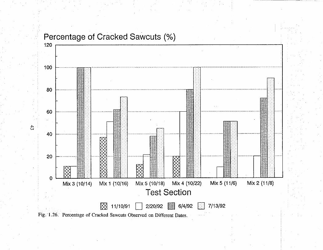
Percentage of Cracked Sawcuts (%) 120 .--~~~~~~~~~~~~~~~~~~~~~~~~~~~---,

100

80 ................... .

60

40

20

Mix 3 (10/14) Mix 1 (10/16) Mix 5 (10/18) Mix 4 (10/22) Mix 5 (11/6) Mix 2 (11/8)

Test Section

~ 11110191 D 2120192 • 6/4/92 D 1113192

Fig. 1.26. Percentage of Cracked Sawcuts Observed on Different Dates.

drying of concrete, and slowed down the hydration of concrete. As a result, small

stresses were induced.

It is interesting to note that the first cracking occurred approximately in the

middle of a one-day placement. The typical examples can be seen in the section of Mix

Design 3, paved on October 14, 1991 (Fig. 1.1), and the section of Mix Design 5,

paved on November 6, 1991 (Fig. 1.6). It is understood that, in the middle of a pour,

stresses caus.ed by curling and friction are larger than elsewhere. Cracks did not grow

simultaneously at every sawcut in the same section but appeared to develop gradually on

a random basis. The cracks which formed early opened widely, such as those cracks

observed in 1991. These widely-opened cracks may have lessened the restraint of the

pavement for stress development, not to mention the diminished load transfer efficiency

at the widened joints. Joint openings should be monitored as additional cracking at

other joints progresses to determine future distributions of the openings.

Percentage of cracked sawcuts on three different dates, February 20, June 4 and

July 13, 1992, is shown in Figs. 1.27 to 1.29 as a function of sawcut type and mix

design. Transverse sawcuts in the sections of Mix Design 4, paved on October 22,

1991 (Fig. 1.8), and of Mix Design 5, paved on November 6, 1991 (Fig. 1.6), were

made with the early-aged technique. Therefore, data shown in Fig. 1.26 for these two

sections are based on the early-aged sawcuts. (These data are not included in Figs.

1.27 to 1.29.) As of February 20, 1992, in two of the four sections referred to in Fig.

1.27 (Mixes 3 and 5), all of the observed cracks occurred at the early-aged sawcuts

while in the other sections, Mix 1 and Mix 2, there were more cracks at the

conventional sawcuts than at the early-aged sawcuts. As of June 4, 1992, in each of the

four sections, there were more cracks at the early-aged sawcut than at the conventional

sawcuts. More than a month later, on July 13, 1992, a greater number of

conventionally made sawcuts had induced cracking than the early-aged sawcuts in

sections in Mix Designs 1 and 2. Except for the section of Mix Design 5, percentages

of cracked early-aged sawcuts and percentages of cracked conventional sawcuts showed

no significant difference in performance as of July 13, 1992 .. The early-aged sawcut

technique did not require a supply of water for blade cooling and probably will result

44

Percentage of Cracked Sawcuts (%)as of 2/20/92 70 ~~~~~~~~~~~~~~~~~~~~~~~~~~~~~~

50 ............................................. ······················

40

30

20

10

Mix 3 (10/14) Mix 1 (10/16) Mix 5 (10/18) Mix 2 (11/8)

Test Section

~ early-aged sawcut l<J conventional sawcut

Fig. I .27. Percentage of Cracked Sawcuts Observed on February 20, 1992.

Percentage of Cracked Sawcuts (%)as of 6/4/92 120 ..--~~~~~~~~~~~~~~~~~~~~~~~~~~~~

100

80 ....... .

60

40

20

Mix 3 (10/14) Mix 1 (10/16) Mix 5 (10/18)

Test Section

~ early-aged sawcut I> I conventional sawcut

Fig. 1.28. Percentage of Cracked Sawcuts Observed on June 4, 1992.

Mix 2 (11/8)

Percentage of Cracked Sawcuts (%)as of 7/13/92 120 .--~~~~~~~~~~~~~~~~~~~~~~~~~~~~-.

Mix 3 (10/14) Mix 1 (10/16) Mix s (10/18)

·Test Section

~ early-aged sawcut 11 conventional sawcut

Fig. 1.29. Percentage of Cracked Sawcuts Observed on July 13, 1992.

Mix 2 (11/8)

in lower blade costs per foot. This method also provided a great deal of convenience in

pavement construction. This technique can be recommended for joint sawcutting in

jointed concrete pavement from the standpoint of performance noted in this project. It

should also be noted that the weather conditions under which most of these test sections

were placed were some of the most-stringent conditions as far as crack control is

concerned. Improved curing techniques may enhance the performance of the early-aged

sawcuts, but all things considered, this early-aged method did very well in controlling

cracking in the pavement system.

1.11. FWD TEST MEASUREMENT OF LOAD TRANSFER EFFICIENCY AND EFFECTIVE MODULUS AT THE JOINTS

FWD (falling weight deflectometer) testing was conducted on several sawcut

joints, construction joints and cracks on the morning of February 20, 1992. Locations

of these joints and cracks are listed in the first column of Table 1.9. The testing

equipment is a trailer-mounted FWD weighing approximately 1,500 pounds (6,670 N).

The impulse force is created by dropping masses. The load, measured by a transducer,

is transmitted to the pavement through a load plate having a radius of 5 .9055 inches

(150 mm). Deflections are measured by using velocity transducers mounted on a bar

that is lowered simultaneously with the load plate to the pavement surface. The loading

plate and deflection sensors layout is on 12-inch (304.8 mm) centers. Eight sensors are

mounted on the bar. One of the sensors measures the deflection at the load, noted as

D0• Six sensors are on one side of the load at 12 inches (304.8 mm), 24 inches (609.6

mm), 36 inches (914.4 mm), 48 inches (1219 mm), 60 inches (1524 mm) and 72 inches

(1829 mm) away from the load position. Deflection measured by these sensors is

designated as Dh D,, D3, D4, D5 and D6, respectively. Another sensor is on the other

side of the load, 12 inches (304.8 mm) away from load. It measures the deflection

noted as D_1•

The results of the FWD field measurements are described in terms of the load

plate deflection (D0), the load transfer efficiency (L TE), and the effective stiffness (Eo)

at the joint. The LTE is equal to the change in deflection on the unloaded side of the

48

Table 1.9. Results of FWD Tests.

Station Mix Design Date of Type of Joint or Crack Downstream Upstream Upstream Effective Stiffness Nnmber Paving LTE (%) LTE (%)

255+51.55 3 10-14-91 earlv-aged sawcut 88.89 No data No data

254+61.3 3-5 construction ioint 82.06 81.28 1154 ksi (7 .957 GPa)

254+41.3 1 10-16-91 early-aged sawcut 81.06 78.18 568 ksi (3.916 GPa)

254+11.5 1 10-16-91 conventional sawcut 78.31 79.36 967 ksi (6.667 GPa) '

253+96.3 1 10-16-91 conventional sawcut 80.20 78.00 ' 571 ksi (3.937 GPa)

253+66.5 1 10-16-91 conventional sawcut 81.96 79.58 559 ksi (3.854 GPa) '

252+ 18.0 5 10-18-91 early-aged sawcut 87.80 79.62 504 ksi (3.475 GPa)

251 +73.0 5 10-18-91 early-aged sawcut 78.99 85.64 1845 ksi (12. 72 GPa)

251 +58.0 5 10-18-91 earlv-aged sawcut 84.16 80.34 776 ksi (5.351 GPa)

250+91.0 5 10-18-91 crack 67.15 82.58 974 ksi (6. 716 GPa)

250+26.8 5 construction ioint 81.05 79.64 770 ksi (5.309 GPa) '

249+2.48 5 10-26-91 crack 84.69 81.09 819 ksi (5.647 GPa) '

248+42.0 5 construction ioint 79.39 82.91 1151 ksi (7.936 GPa) '

247+41.7 5 11-6-91 earlv-aged sawcut 80.79 77.68 2694 ksi (18.58 GPa) '

246+51.4 5-2 construction joint 87.11 78.14 998 ksi (6.881 GPa)

245+83.l 2 11-8-91 earlv-aged sawcut 85.97 89.28 1475 ksi (10.17 GPa) '

245+53.l 2 11-8-91 early-aged sawcut 85.86 88.08 1788 ksi (12.33 GPa)

244+33.l 2 11-8-91 conventional sawcut 89.74 85.56 1433 ksi (9.881 GPa)

243+88.1 2 11-8-91 conventional sawcut 87.65 85.55 1252 ksi (8.633 GPa)

243+9.l 2-4 construction ioint 87.17 87.35 1475 ksi (10.17 GPa)

242+74.6 4 10-23-91 early-aged sawcut 99.73 86.52 1384 ksi (9.543 GPa)

242+4.41 4 10-23-91 early-aged sawcut 92.92 87.44 1738 ksi (ll.98GPa)

241+31.6 4 10-23-91 early-aged sawcut 88.10 94.67 4208 ksi (29.01 GPa) , i

'

joint divided by the change in deflection on the loaded side of the joint. The effective

-------------------------- stiffnessE0 is-determined-from-the-Westergaard solution forslabcon-grade deflections at

an interior load position. The simplified form of the Westergaard solution rearranged to

solve for the modulus of subgrade reaction K (assuming Poisson's ratioµ = 0.15 for

concrete) is:

[l - (~)2 (0.217 - 0.367 log~)]

fK fK (1.1)

where Pis the applied load, a is the radius of the FWD load plate (150 mm), and fk is

the radius of relative stiffness of the slab based on the area basin. It leads to

E, = K(fJ4 (ll.73)/h 3 (1.2)

where h is the pavement thickness and f k can be determined from the deflection basin

area through the Westergaard solution or the computer program ILLISLAB.

The deflection basin area is defined as (Fig. 1.30).

(1.3)

The FWD was equipped with seven channels for deflection recording.

Deflections D_h D0, DI> D2, D4 , D5, and D6 were recorded in the FWD tests on the test

sections. Since D3 was not recorded, D3 in Eq. (1.3) was replaced by 1/2(D2 + D4) in

calculating the basin area.

In all the tests, the sensor for D_1 was on the downstream side of the joint or

crack while the sensors for D1 through D6 were on the upstream side. Therefore, when

the load acted on the upstream side of the joint or crack, the downstream LTE value

was obtained as LTD = D/D0 • When the load was acted on the downstream side of

the joint or crack, the upstream LTE was obtained as LTD = D_/D0• The deflection

basin area was determined when the load was placed on the upstream side of the joint or

50

15 cm

P • FWD Impulse Load

30->5 cm 61 cm !H.5 cm

(12") (24") 36") ..,,_.1...1.-+..:....l-'-~~~~~...;,,_r-~~~~~~......:....~~~~~~~--'~

l

2

3

5

6

Dl DZ

6 Area (in.) = D [D0 + 2D1 + 2Dz + D3)

0

Fig. l.3Q. Basin Area Measurement from' FWD Test.

D3

----·•--,-._ ____ .

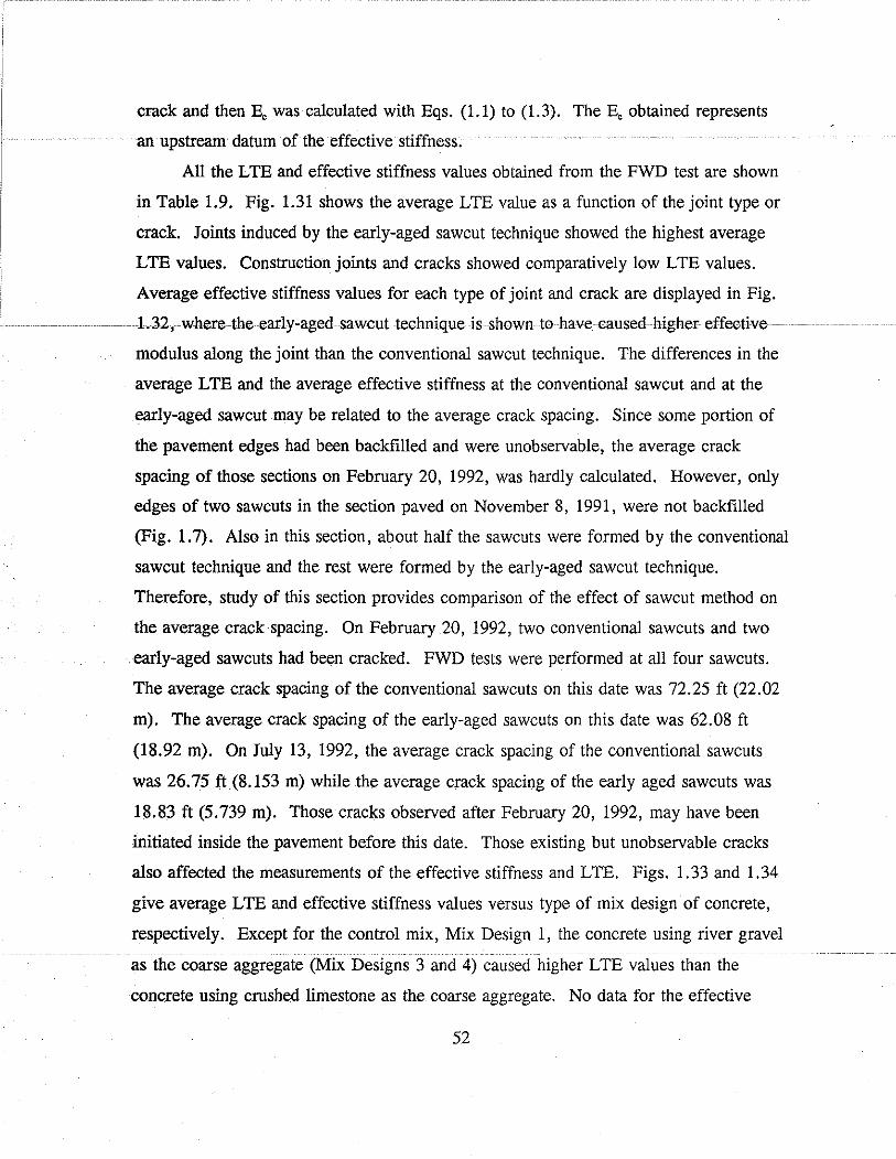
crack and then E, was calculated with Eqs. (1.1) to (1.3). The E, obtained represents

an upstream datum of the effective stiffness.

All the LTE and effective stiffness values obtained from the FWD test are shown

in Table 1.9. Fig. 1.31 shows the average LTE value as a function of the joint type or

crack. Joints induced by the early-aged sawcut technique showed the highest average

LTE values. Construction joints and cracks showed comparatively low LTE values.

Average effective stiffness values for each type of joint and crack are displayed in Fig.

-------- - - --- - -- --L32, where the early-aged sawcut technique is shown to have caused higher effective

modulus along the joint than the conventional sawcut technique. The differences in the

average LTE and the average effective stiffness at the conventional sawcut and at the

early-aged sawcut may be related to the average crack spacing. Since some portion of

the pavement edges had been backfilled and were unobservable, the average crack

spacing of those sections on February 20, 1992, was hardly calculated. However, only

edges of two sawcuts in the section paved on November 8, 1991, were not backfilled

(Fig. 1.7). Also in this section, about half the sawcuts were formed by the conventional

sawcut technique and the rest were formed by the early-aged sawcut technique.

Therefore, study of this section provides comparison of the effect of sawcut method on

the average crack spacing. On February 20, 1992, two conventional sawcuts and two

early-aged sawcuts had been cracked. FWD tests were performed at all four sawcuts.

The average crack spacing of the conventional sawcuts on this date was 72.25 ft (22.02

m). The average crack spacing of the early-aged sawcuts on this date was 62.08 ft

(18.92 m). On July 13, 1992, the average crack spacing of the conventional sawcuts

was 26. 75 ft (8.153 m) while the average crack spacing of the early aged sawcuts was

18.83 ft (5.739 m). Those cracks observed after February 20, 1992, may have been

initiated inside the pavement before this date. Those existing but unobservable cracks

also affected the measurements of the effective stiffness and LTE. Figs. 1.33 and 1.34

give average LTE and effective stiffness values versus type of mix design of concrete,

respectively. Except for the control mix, Mix Design 1, the concrete using river gravel

as the coarse aggregate (Mix Designs 3 and 4) caused higher LTE values than the

concrete using crushed limestone as the coarse aggregate. No data for the effective

52

Average LTE (%) 100 r-~~~~~~~~~~~~~~~~~~~-'--~~~~........,.....,

83.6

80 80.2 80

60

C'.l 40

20

early-aged sawcut conventional sawcut construction joint

Type of Joint or Crack ~ downstream. H j upstream

Fig. 1.31. Average Load Transfer Efficiency at Joints and Cracks.

81.8

crack

Average of Effective Stiffness (GPa) 12

10 f- .......................... 9.78

x

vvvvv~x Vv'v'Vv ',)'\

" J>( x;;o 8 i.- .......•.... .... Vv' '\.'\.•'''')("}('

xx ..................... .. ................................ ].8(1

6 I-········ xx

Vvv v'Vv' IJVv'v"' ,,,('}(Vv IJy'I./ x :)< 4 f- ................ K X '\. "V\ X..X, X...X.

2 -

0

n. ')'\.I'\ I\~ 1\,1\

v::>Ovvvvvv

t'\1\1\A, \l"",f'\A

·t'\1\1\A,AA'\.,I\ t'\1\1\"'\X.Xl'\I\ t) I\/\ I\ X/\ I\ I\,...,, " " "><"> ~'><V' N > XXX.XI\~)(

",'Vv '"

6.59 · """="""x"vv=v"'v""

,/..;~;~Xvvvv

Vvv v '>(")('J('./

>('"\'\.l'\.X..XA. '\.'\.l'\l'\~X.. ''v''v'\. "'" ·v ·v '

................................... AA vVvvvv Al\ V v'Vv'V

x:>< 'V\ '\'\

IO >0o:;K><"8>;::c;::>01

early-aged sawcut conventional sawcut

,;() v 'X..1\1\ " ,/ .t .t 'X " 'V'\ .x.. v v v v " '.)() : :x

vVvv v~~ Q~ 'V)()(VV

construction joint

Type of Joint or Crack Fig. 1.32. Average Effective Stiffness at Joints and Cracks.

6.18

r-.,0 VVvvvv

v x ><Xr'l'' V '' '"l''lrJA

.............. ~ ~~~:~~~,..., .. Y~'V'\:')""l""lr'l

v "\'.')( : )"''1'')0 v '\.A,I'\

,.?,X,.x X

crack

--------·~---.------···-----_,. __ _

LTE(%) 100

l&.2Yol

11.0'Yo) (1.7%1

80

60

~ 40

20

0 Mix 1 [e] Mix 1 [n] Mix 2 [e] Mix 2 [n] Mix 3 [e] Mix 4 [e] Mix 5 [e]

t;s downstream • upstream

Mix Design !el early-aged sawcut lnl conventional sawcut

( ) c.v. of average L TE L TE value from a slgle Joint with no c.v. noted

Fig. 1.33. Average Load Transfer Efficiency at Joints Formed by Early-Aged and Conventional Sawcut Techniques.

Effective Stiffness (GPa) 12 .-~~~~~~~~~~~~~~~~~~~~~~~~~~~~~~~~

10

8

6 ·······················

(13.5%)

(33.2%)

Mix 1 Mix2

Mix Design Mix4

( ) c.v. of average L TE L TE value from a single joint with no c.v. noted

(12.3%)

Mix5

~ early-aged sawcut li!itil conventional sawcut [a crack

Fig. 1.34. Average Effective Stiffness at Joints Formed by Early-Aged and Conventional Sawcut Techniques.

stiffness along joints in the test section of Mix Design 3 were acquired. However, it is

···················· shownthatMixDesign-4provided-highereffectivestiffness values than Mix Design 5.

Mix Design 2, replacing part of crushed limestone by 0.75 inch (19 mm) river gravel,

provided even higher LTE and effective stiffness than Mix Design 5. These differences

for sections of different mix design may also be explained by the average crack spacing.

The average crack spacings of the early-aged sawcut sections of Mix Designs 2, 4 and 5

The advantage of river gravel for the joint load transfer can be attributed to its

fracture behavior in concrete. Limestone is softer and may break during fracturing of

the concrete. In contrast, river gravel is very hard. The fracture toughness of river

gravel is higher than that of mortar as well as the interface between river gravel and

mortar. When concrete using river gravel as the coarse aggregate fractures, the fracture

surface goes around the river gravel aggregates. Therefore, in the pavement of river

gravel concrete, the joint surface, formed by fracturing from the sawcut, is tortuous.

Hard river gravel aggregates protrude from both sides of the joint and interlock one

another. More gravel interlocking provides better performance of joint in transferring

load across the joint are listed in Table 1.10 for comparison.

Table 1.10. Average Crack Spacings of the Early-Aged Sawcut Part.

Average Crack Spacing

Mix Paving Date February 20, 1992 July 13, 1992

2 November 8, 1991 62 ft (19 m) 19 ft (5.8 m)

4 October 22, 1991 36ft(llm) 18 ft (5.5 m)

5 November 6, 1991 95 ft (29 m) 32 ft (10 m)

1.12. CONCLUSIONS AND RECOMMENDATIONS

1. A jointed concrete pavement test section was placed in Texarkana, Texas, for

experimental studies in concrete placement, joint formation, and crack control. Five

57

different mix designs of concrete (using different coarse aggregates: crushed limestone,

river. gravel, or blends of both) and different curing methods were applied to different

sections of the pavement to compare their influences on performance of the pavement.

Two sawcut techniques, the conventional and the early-aged, were used for formation of

the joint. Temperature and relative humidity in these sections were monitored. Cracks

were surveyed eight times during the period of nine months after paving. It was found

that differences made by different mix designs, curing methods and sawcut techniques

were obvious, which made it clear that such field tests are useful in helping to

understand the effects of coarse aggregates, curing methods and sawcut techniques.

2. Early cracking at the sawcut tip occurred more frequently in sections of river

gravel concrete (Mix Designs 1, 3 and 4) than in sections of crushed-limestone concrete

(Mix Design 5). It also occurred more frequently in the concrete that consisted of a

blend of crushed limestone and river gravel as the coarse aggregate (Mix Design 2) than

concrete that used only pure crushed limestone purely as the aggregate (Mix Design 5).

Concrete of the control mix design that used 1.5-inch (38 mm) river gravel as the

coarse aggregate (Mix Design 1) was improved by adding buckshot as the intermediate

aggregate. The improved mix design (Mix Design 3) was better than the control mix

design in formation of controlled cracks. Another mix design (Mix Design 4) that used

0. 75-inch (19 mm) river gravel as the coarse aggregate and buckshot as the intermediate

aggregate also showed better performance in formation of control cracks than the

control mix design.

3. Lab tests showed that concrete of crushed limestone had higher flexural and

compressive strengths than concrete of river gravel. This may explain why cracks were

more likely to grow in river-gravel concrete. Also, smaller aggregates may have

lowered the strength of the concrete and increased the tendency to crack. However,

strength cannot explain why Mix Design 3 performed better in formation of controlled

cracks than Mix Design 1. From both lab specimen and cored specimen tests, Mix

Design 3 had higher compressive and tensile strengths than Mix Design 1. As observed

in crack surveys, some cracks occurred within one or two days after paving while

formation of some other cracks took a period as long as 9 months. For the cracks that

58

formed at the early ages of concrete, an analysis is included in Chapter 5. For those

delayed cracks, further study is needed. In the delayed fracture process, effects of

creep and fatigue may be important aspects.

4. There were two uncontrolled transverse cracks in the whole test section

pavement. Both of them were initiated from a blockout corner where stress

concentration existed. It is suggested that such stress-concentration causing sharp

comers should be avoided in design or a joint (sawcut) should be located to connect to

any sharp corner to control cracking. A random longitudinal crack was observed

alongside a part of the longitudinal sawcut, which was formed with the conventional

sawcut technique, although the cause is not clear yet.

5. The early-aged sawcut technique has the capability to be applied to pavement

earlier than the conventional sawcut technique so that controlled cracks were formed

earlier. With the early-aged sawcut method, the depth of c.ut was 1 inch (25 mm),

much less than D/4 to D/3 as used for the conventional sawcutting of joints. In

addition, the early-aged method did not require a supply of water for cooling saw

blades. These advantages of the early-aged sawcut technique provided great

convenience in construction. In this study, minimal raveling occurred along with the

early-aged sawcutting operations. Data showed that the operations can be arranged

when the pulse velocity reaches the order of 3600 - 4600 feet/sec (1110 - 1400 m/sec).

6. FWD tests were conducted at some of the joints where cracking had occurred

at the sawcut tip and developed through the pavement bottom surface, as well as at the

construction joints and the two uncontrolled transverse cracks. The tests were

conducted in order to obtain the load transfer efficiency and effective stiffness at these

locations. Sawcutting formed joints were found to have higher load transfer efficiencies

and higher effective stiffness than construction joints and uncontrolled cracks on the

average. The early-aged sawcutting provided higher load transfer efficiency and higher

effective stiffness than the conventional sawcutting. One apparent reason is that the

early-aged sawcut was 2 inches (51 mm) shallower than the conventional sawcut so that

a 2-inch longer zig-zag fracture surface existed at the joint by the early-aged sawcutting

providing more aggregate interlocking. A wide crack opening may have occurred at the

59

joint by the conventional sawcutting. However, it is not yet clear since the crack

opening was not measured with an instrument any better than a common ruler.

Although the crushed-limestone concrete had higher compressive and tensile strengths

than the river gravel concrete, the crushed-limestone concrete did not provide higher

load transfer efficiency. It may be due to different behaviors of limestone and river

gravel in concrete fracturing. River gravel does not break when concrete fractures, so

it provides better aggregate interlocking. With intermediate aggregate in concrete,

aggregate interlocking would be improved, and therefore, load transfer performance at

the joint would be improved.

7. The strength of concrete in the pavement not only depends on the mix design,

but also on construction operation. From tests on specimens prepared in the laboratory,

compressive and flexural tension strengths of concrete of Mix Design 2 were

comparatively high while the split tension strengths of the cored specimen of Mix

Design 2 were comparatively low. The most serious air pockets were observed in the

cored specimen of Mix Design 2.

8. Split tension tests on specimens from the same core but at different depths in

the pavement showed that the tensile strength increased with depth. This indicates that

concrete is not homogeneous through the pavement depth. Inhomogeneity in concrete

properties along the pavement depth would be a significant factor in stress analysis in

the pavement. Further experimental investigation of this phenomenon is needed.

9. In comparison with the membrane curing method (using standard white

pigments or Procrete), cotton mat and polyethylene film both slowed down the drying

process in pavement concrete. When the daily average ambient temperature dropped

from the day of the paving, the wet cotton mat may have helped cool the pavement, and

therefore, maintained the mat covered pavement at a lower temperature than the

membrane cured pavement. The polyethylene film covering the pavement formed a

"greenhouse" effect over the pavement, which made the temperature in the pavement

higher than in the pavement cured with the membrane method. When there was sun

and the daily average ambient temperature increased after the day of paving, pavement

with neither cotton mat nor polyethylene film covering absorbed more solar radiation,

60

and therefore, temperature was higher than that in pavement covered with cotton mat or

polyethylene film.

1.13. APPENDIX: MIX DESIGN USED IN THE TEST SECTIONS

The 5 mix designs with mix analysis, aggregates gradation, all-components

gradation and material distribution by sieve are given in this appendix. Terms used in

analysis are defined as follows.

Q - The plus 3/8-inch (9.5 mm) sieve particles are the high quality, insert

filler sizes.

I - The minus 3/8-inch (9.5 mm), plus No. 8 (2.36 mm) sieve particles are

the intermediate particles that fill major voids and aid in mix mobility,

or, if elongated and sharp, interference particles that contribute to mix

harshness.

W - The minus No. 8 (2.36 mm) sieve particles give the mixture workability.

Coarseness - It is defined as Q/(Q+ I).

Workability-Adjusted - The amount of fine aggregate needed is influenced by the

amount of cementitious materials. As cement content is varied, the sand content should

be adjusted. One 94-lb (42.6 kg) US bag of cement is equal to approximately 2.5

percent of the combined aggregate. Workability = Workability-Adjusted when the

cement factor is 6 bags. If the cement factor is higher than 6 bags, Workability

Adjusted will be higher than Workability and vice versa.

The mix designs were made by following the Construction Bulletin issued by the

Texas Department of Transportation.

61

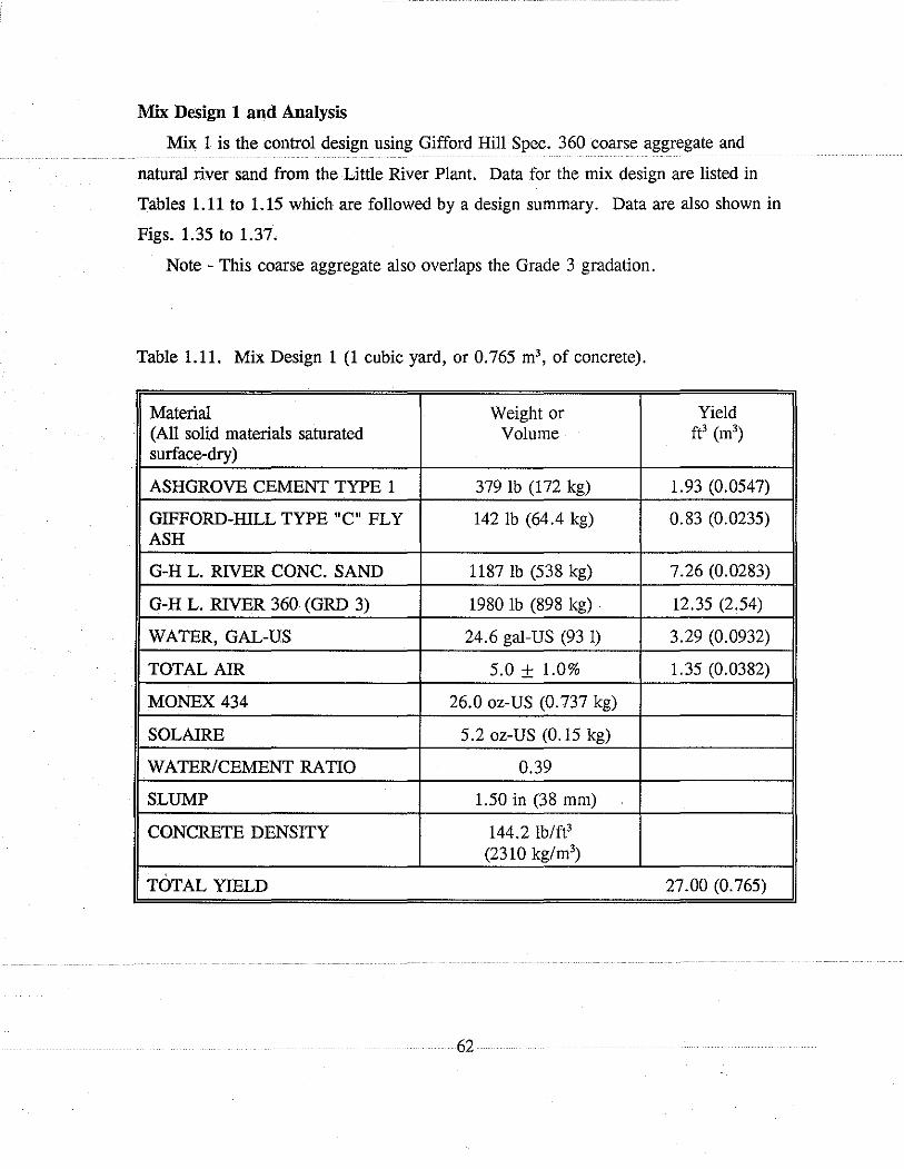
Mix Design 1 and Analysis

Mix 1 is the control design using Gifford Hill Spec. 360 coarse aggregate and

natural river sand from the Little River Plant. Data for the mix design are listed in

Tables 1.11to1.15 which are followed by a design summary. Data are also shown in

Figs. 1.35 to 1.37.

Note - This coarse aggregate also overlaps the Grade 3 gradation.

Table 1.11. Mix Design 1 (1 cubic yard, or 0.765 m3, of concrete).

Material Weight or Yield (All solid materials saturated Volume ft3 (m3

)

surface-dry)

ASHGROVE CEMENT TYPE 1 379 lb (172 kg) 1.93 (0.0547)

GIFFORD-HILL TYPE "C" FLY 142 lb (64.4 kg) 0.83 (0.0235) ASH

G-H L. RIVER CONC. SAND 1187 lb (538 kg) 7.26 (0.0283)

G-H L. RIVER 360 (GRD 3) 1980 lb (898 kg) 12.35 (2.54)

WATER, GAL-US 24.6 gal-US (93 1) 3.29 (0.0932)

TOTAL AIR 5.0 ± 1.0% 1.35 (0.0382)

MONEX 434 26.0 oz-US (0.737 kg)

SOLAIRE 5.2 oz-US (0.15 kg)

WATER/CEMENT RATIO 0.39

SLUMP 1.50 in (38 mm)

CONCRETE DENSITY 144.2 lb/ft3

(2310 kg/m3)

TOTAL YIELD 27.00 (0.765)

62

Table 1.12. Mix Analysis of Mix Design 1.

MIX VOLUME (ft3) 27.00 (0.765 m3)

COARSENESS (Q/(Q+I)) 31.3

WORKABILITY 30.2

W-ADJUST 29.0

PERCENT MORTAR 49.2

TOTAL FINENESS MODULUS 5.56

Note - Fig. 1.35 shows the Workability vs. the Coarseness.

Table 1.13. Materials Characteristics for Mix Design 1.

SRG SAND

SPECIFIC GRAVITY 2.57 2.62

% PASSING 3/8" (9.5 mm) 9.9 100.0 SIEVE

% PASSING # 8 SIEVE 0.1 81.8

FINENESS OF AGGREGATE 7.22 2.75

PERCENT OF AGGREGATE 63.0 37.0

MINERAL ADMIXTURE, SPECIFIC 2.75 GRAVITY

63

Table 1.14. Full Gradation Analysis of Mix Design 1.

SIEVE SRG SAND PASTE TOTAL AGGR

1 1/2" (38 mm) 100.0 100.0 100.0

l" (25 mm) 90.l 95.5 93.8

3/4" (19 mm) 68.0 85.4 79.8

1/2" (12.7 mm) 31.2 68.5 56.7

3/8" (9.5 mm) 9.9 100.0 58.8 43.3

# 4 0.5 98.5 54.1 36.8

# 8 0.1 81.3 49.3 30.2

# 16 - 70.2 46.3 26.0

# 30 - 57.6 42.9 21.8

# 50 - 16.6 31.8 6.1

# 100 - 0.9 27.6 0.3

# 200 - 0.1 100.0 27.4 0.0

# 325 - - 95.5 26.2 -

Liquid - - 62.8 17.2 -

Note - Fig. 1.36 shows the Gradation Analysis.

64

Table 1.15. Materials Distribution of Mix Design 1.

SIEVE SRG SAND PASTE TOTAL AGGR

1 1/2" (38 mm) 100.0 0.0 -

1" (25 mm) 90.1 4.5 6.2

3/4" (19 mm) 68.0 10.1 13.9

1/2" (12.7 mm) 31.2 16.8 23.2

I 3/8" (9.5 mm) 9.9 100.0 9.7 13.4

# 4 0.5 98.5 4.7 6.5

# 8 0.1 81.3 4.8 6.6

# 16 - 70.2 3.0 4.2

# 30 - 57.6 3.4 4.7

# 50 - 16.6 11.0 15.2

# 100 - 0.9 4.2 5.8

# 200 - 0.1 100.0 0.2 0.3

# 325 - - 95.5 1.3 0.0

Liquid - - 62.8 9.0 -

Note - Fig. 1.37 shows the Materials Distribution of Sieve.

65

DESIGN SUMMARY FOR MIX 1

DESIGN COMPRESSIVE STRENGTH: 4550 PSI (31.4 MPa) EQUIVALENT FLEXURAL STRENGTH: 700 PSI (4.83 MPa)

MAXIMUM AGGREGATE SIZE AGGREGATE SHAPE 1 1/2 IN (38 mm) NATURAL GRAVEL

TOTAL AIR: 5.00% +/-1.00

WATER METHOD: AMOUNT:

CEMENT METHOD: AMOUNT: W/C

541 4.3

MINERAL ADDITIVE METHOD: ADDITIVE 1: 142

SEVERE EXPOSURE CONDITIONS NO SEVERE EXPOSURE

COARSE AGGREGATE ACI bbo W-ADJUST TOTAL FM

SRG

METHOD:

29.0 5.56

AMOUNT 1980 LB (898

FINE AGGREGATE METHOD: SAND AMOUNT

kg)

1187 LB (538 kg)

MIX VOLUME:

66

SLUMP: 1.50 IN (38 mm)

MANUAL ENTRY 24.6 GAL-US (93 liters)

MANUAL ENTRY (379] LB (172 kg) (4.4] GAL/SK (16.7 liters)

REPLACEMENT BY VOLUME (142] LB (64.4 kg)

W-ADJUST WORKABILITY FACTOR PERCENT STONE 63.0 PERCENT MORTAR 49.3 NRMCA FM FINENESS MODULUS

7.22

PRODUCE A SPECIFIC VOLUME FINENESS MODULUS

2.75

27.00 CU FT (0.765 m3 )

-- ""------------"

Mix Analysis 45 ~-----~------r------~-----~----~

40 -+-------+-------+------+------+-------!

~ -·--·-.!2 m ~ :i..

0\ 0 --i 3:

... :.;.:.:.:··· :.;.,.:.•

25 -+-~-'--'--'-"''----+-------+-------+------+-------j

100 80 60 40 20 0

Coarseness ID Workability <> Workability - Adjusted

Fig. 1.35. Workbility versus Coarseness of Mix Design !.

Gradation Chart 100 --~~-,-~~~-,-~~~-,-~~~~~~~~~~~~~~~~~~~~~~~~~~

$ 90 - . . ........ , .. : ... , ... ·············•· ·····; ···············'···· ....... , .. . .............. \······· ·····r· .............. 1··· .................... ·····1··· .. ······· .. : ...

C> c ·-en

80 - ············ 1 ....

I =

70 - ............... r····r .. . ······j ............... r·· .. 1 .......

····~ ....... T ..

·•·!········· ·······\·· ······················· ···1············

·r· .. "''\"' ··········1······· ·········t ..

en C'IS a.

60 - ..... • • $ 6 : .................. . ···········j··················; ························· '''\''

-c Cl)

50 - ........ ........ ! . f .............. ~ .t ...................... .

"' 0 00 a.. .............. ;········"··· .. ·······"! 40 - : ! i ·······!····· .. ...... : .............................. .

Cl) a. 30 - ................. ; ...... ; ................ !····· '··················· ···~··· . ...... !··· ...

4 ................ ; ...... . .. ; ..

4 .. .. ; ...

20 - ................ . . . ·~ ...... ·~ ····<;>·-- ""·i

10 - .... ............ !·· ···············-:-····· ......... ~--··· ...

~ .. ... .. .. ... . .. .. .. .. . . .... j" ........ ...... ... . .. ·~

0 -\-~~-i--1 -i--1 ~--i-1 ~i--1 ~--i--1 ~~~i--,~~~i--1 ~~~i--1 ~-+-,~~~--1Tll-~~--1;~·~~,Elil-l 1.5 1 3/4 1/2 3/8 >114 >118 >1116 >1130 >1150 •100 >11200 >11325

Sieve 111 Aggregates 4 All Components

Fig. 1.36. Full Gradation of Mix Design I.

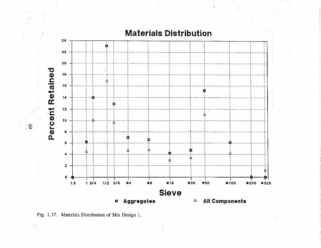
0\ \0

'tJ G> r::: ·-ca ..... G> a: ..... . r:::

G> 0 I.. G> a..

\

Materials Distribution 24

Iii 22 - .......... ...... !. '''''1"'' .. r ..... : ............... r .. ······· ............. 1··················· ...... I

.

.......... i ···········1 .. ····· ........ : .. .

......... ! ...... ~ ............... ·! ...... ! ............... l ....................... i .. . ':

20 - .......... j .. . .............. !·· ··············!···· ............... !

. . ! T ; ; i + +· . . r +· . i .. . .;

+~····Ji···········.... !·············· : il; <······ T

18 -

16 -

14 -

12 - .....................

A 10 - : + r i · r ···········j··· ...................... : ......................... , .. ' .. : . ' i

"1·········· ····················!·················· ·······i··· ············!··· !

·······!······· ·········i········· ···················~···················· ··-~········· ······!···

l i .. 1 .... , L

i + ,. :· ··; . ·~· . !

: ; ·r ; 1··········~·· .. I T ' T j ; . i .; .

4'

8 -

6 -

4 - ....

...... ·!·

* ......... t· ' : : ·······················:···· ....................... l:1····························1··· .. ···· ························r··

l i. 0 -8-r-~T--,~l~~~,~;..-,~-;..-,~~-+,~~~-;..-,~~--;l~~;l~~~~;,c--~~;,11-~-Tiil-1

2 - ................. .

1.5 1 3/4 1/2 3/8 !t4 !t8 !t16 !t30 !t50 •100 •200 !t325

Sieve 111 Aggregates a All Components

Fig. 1.37. Materials Distribution of Mix Design I.


Mix 2 is a design using a 50/50% blend of 1 1/2-inch (38 mm) crushed Limestone

and 3/4-inch (19 mm) SRG from the Gifford Hill Delight Plant; Gifford Hill Buckshot

from the Hoot Plant; 65% Gifford Hill crushed sand; and 35% concrete sand from

Little River. Data for the mix design are listed in Tables 1.16 to 1.20, followed by a

design summary. Data are also shown in Figs. 1.38 to 1.40.

Table 1.16. Mix Design 2 (1 cubic yard, or 0.765m3, of concrete).

Material Weight or Yield (All solid materials saturated Volume ft' (m3

)

surface-drv)



G-HHOOT 379 lb (172 kg) 2.35 (0.0666) PLANT/BUCKSHOT, LB

G-H LITTLE RIVER/CRUSHED 740 lb (336 kg) 4.58 (0.130) SAND

G-H LITTLE CONCRETE SAND 403 lb (183 kg) 2 .46 (0. 0697)

G-H 1 1/2" (38 mm) CRUSHED 857 lb (389 kg) 5.11 (0.145) LIMESTONE

G-H DELIGHT PLANT 3/4" 826 lb (375 kg) 5.11 (0.145) (19 mm) SRG

WATER 24.6 !!al-US (93 1) 3.29 (0.0932)

TOTAL AIR 5.0 +% 1.35 (0.0382)

MONEX 434 26.0 oz-US (0. 737 kg)




CONCRETE UNIT WEIGHT 145.6 (lb/ft') (2330 kg/m3)


70


MIX VOLUME 27.00 ft3 (0.765 m3)


WORKABILITY 32.7 .

W-ADJUST 31.5

PERCENT MORTAR 51.1



Table 1.18. Material Characteristics for Mix Design 2.

LIMESTONE SRG BUCKSHOT CRUSHED CONCRETE SAND SAND

DENSITY SPECIFIC GRAVITY 2.69 2.59 2.59 2.59 2.59

% PASSING 3/8" (9.5 mm) 17.7 38.0 100.0 100.0 100.0 SIEVE

% PASSING # 8 SIEVE 0.6 1.0 13.1 87.6 81.3

FINENESS MODULUS 7.32 6.60 4.86 2.82 2.75

PERCENT OF AGGREGATE 26.1 26.1 12.0 28.4 12.4

MINERAL ADMIXTURE, SPECIFIC GRAVITY 2.75

71


SIEVE LIMESTONE SRO BUCKSHOT CRUSHED CONCRETE PASTE TOTAL AGOR SAND SAND

1 1/2" (38 mm) 100.0 100.0 100

l" (25 mm) 75.9 100.0 95.4 93.6

3/4" (19 mm) 47.6 96.0 89.3 85.0

1/2" (12.7 mm) 31.2 59.0 79.2 71.0

3/8" (9.5 mm) 17.7 38.0 100.0 100.0 100.0 72.7 62.0

# 4 2.1 5.0 85.8 99.5 98.5 62.1 47.4

# 8 0.6 1.0 13.l 87.6 81.3 51.1 32.4

# 16 - - 6.8 60.5 70.2 44.6 23.6

# 30 - - 5.5 38.6 57.6 39.7 16.8

# 50 - - 2.1 22.6 16.6 32.9 7.6

# 100 - - 0.4 9.6 0.9 29.1 2.4

# 200 - - 0.1 3.3 0.1 100.0 28.0 0.5

# 325 - - - - - 95.5 26.2 0

Liquid - - - - - 62.8 17.2 0


72


SIEVE LIMESTONE SRO BUCKSHOT CRUSHED CONCRETE PASTE TOTAL AGOR SAND SAND

11/2" 100.0 0.0 0 (38 mm)

1" 75.9 100.0 4.6 6.4 (25 mm)

3/4' 47.6 96.0 6. I 8.6 (19 mm)

1/2" 31.2 59.0 IO. I I3.9 (12.7 mm)

3/8" 17.7 38.0 100.0 100.0 IOO.O 6.5 9.0 (9.5 mm)

# 4 2.1 5.0 85.8 99.6 98.5 10.6 I4.6

# 8 . ..

0.6 1.0 ... 13.J. 87.6 81.3 .. . .. . . I 1.0 I5.0 ..

# 16 - - 6.8 60.5 70.2 6.5 8.8

# 30 - - 5.5 38.6 57.6 5.0 6.7

# 50 - - 2.1 22.6 16.6 6.8 9.3

# 100 - - 0.4 9.6 0.9 3.8 5.2

# 200 - - 0.1 3.3 0.1 100.0 1.2 1.8

# 325 - - - - - 95.5 1.8 0.6

Liquid - - - - - 62.8 9.0 0

Note - Fig. 1.40 shows the Materials Distribution by Sieve.

73


DESIGN COMPRESSIVE STRENGTH: EQUIVALENT FLEXURAL STRENGTH:

MAXIMUM AGGREGATE SIZE 1 1/2 IN (38 mm)

TOTAL AIR: 5.00% +/-1.00


CEMENT METHOD: AMOUNT: W/C

541 4.3




LIMESTONE SRG

METHOD:

31. 5 5.21

AMOUNT 857 LB (389 826 LB (375

FINE AGGREGATE METHOD:

BUCKSHOT CRUSHED SAND CONCRETE SAND

AMOUNT 379 LB (172 740 LB (336 403 LB (183

kg) kg)

kg) kg) kg)

MIX VOLUME:

74

550 PSI (31.4 MPa) 700 PSI (4.83 MPa)

AGGREGATE SHAPE NATURAL GRAVEL



MANUAL ENTRY [379] LB (172 kg) [4.4] GAL/SK

REPLACEMENT BY VOLUME [142] LB (64.4 kg)

W-ADJUST WORKABILITY FACTOR PERCENT STONE 52.1 PERCENT MORTAR 51.1

NRMCA FM FINENESS MODULUS

7.32 6.60

PRODUCE A SPECIFIC FINENESS MODULUS

4.86 2.82 2.75

VOLUME

27.00 CU FT (0.765 m3)



MAXIMUM AGGREGATE SIZE 1 1/2 IN (38 mm)

TOTAL AIR: 5.00% +/-1.00


CEMENT METHOD:

AMOUNT: W/C liters/sk)

541 4.3




METHOD:

31. 0 5.28

AMOUNT SRG BUCKSHOT

1618 LB (734 kg) 408 LB (185 kg)

FINE AGGREGATE METHOD: AMOUNT

CRUSHED SAND 735 LB (333 kg) CONCRETE SAND 400 LB (181 kg)

MIX VOLUME:

82

4550 PSI (31.4 MPa) 700 PSI (4.83 MPa)


SLUMP: 1.50 IN {38 mm)


MANUAL ENTRY

(379) LB (172 kg) (4.4) GAL/SK (16.7

REPLACEMENT BY VOLUME [142) LB


7.11 4.86

PRODUCE A SPECIFIC VOLUME FINENESS MODULUS

2.81 2.75

27. 00 CU FT (0. 765 m3)

__ ,, -----~"--•-,M•-•••• ••--••-

Mix Analysis

40

>. -·-- 35 ·-.Q m

.ll:: El :i.. .• <;>.··,";' 0 30

.. ·:·:·· . 00

== w

25 -'"'-''-"-'-'-'-'"'-'~'------+------+------.\-------\---------1

100 80 60 40 20 0

Coarseness 111 Workability o Workability - Adjusted

Fig. 1.41. Workbility versus Coarseness of Mix Design 3.

00 ~

en c ·-U) U) ca a. -c Q) () ... Q) a.

100

90 -

80 -

70 -

60 -

50 -

40 -

30 -

20 -

10 -

Gradation Chart

A Iii

········ii-·········· , ... iii

' + .......... i ...... ! ............... \ ... . 4

········; ·········· • +.······ ......... , i u

' ' 'l l ····l··· ...... : ......... ~

'

.................. j .. ......... +···

............. ; .... ··············)····

.............. !

............. 1

A .......... ! ······:···· .. ··· ······r············· .......... ! ·························:······

Iii ...... l ············!

T : T ············:······ ' .

.... .......... : ...... ;... ····+""'

................ , ........ ........ :··· ···············:

. ............... i '

..................................... , .... (

............. , ....... i ............................ , •.•.

............................ ······••(·•

4 ··+···· .. ········!

..... , ..... ·····1·······

······~

, ........... = ........... ········•···

···········j···· ........ +·· '

................. ; .............. 1···

......... , ...

' ......... :

··!·" ............ .

.... ; ........ ······+·· 4

' ... 1 .............. '\' ..

. 1, ........ ,........... .·. ii.

ri. ..i.. 0 -+-~~,i--+--l~-+-,-i--,~-i--1~~--;--,~~~,i--~~-+--,~--;,~~~~-i-l~~--Jlll-l~~Tlll-

1.5 1 3/4 1/2 3/8 #4 #8 #16 #30 #50 #100 #200 #325

Sieve 111 Aggregates A All Components

Fig. 1.42. Full Gradation of Mix Design 3.

Materials Distribution 24 ,-~---,,-~~--,--,-~~,---~~-,-~~~~~~-,-~~,..-~~,---,--~~---,~~~

22 - ... '""'i"' ' .......... , ., .. , ..... !... ,...... ·: ............. .! 1 ·

20 - ................. i ··· .. ·1 ................ ! ······! ................ , ························!···· ············! ........................ !·····

: i ..... ; .... : l i

i ! ··············~ ' ............... , •

........ ·- .......................... i.······ I . . .... , . · Iii .............. ,.

4>

........... i ···············=···

... ; .... ! .................. ·······i,,

i .. ~

·······••:••······················••!.

'tJ Cl) 18 -

r: ·- 16 -ca -Cl) 14 -a: - 12 -r:

00 Cl) 10 -Ul

0 II. Cl) 8 -

a.

·······!··· "'l"···· .. ···· ' .

: T

····················1 ············ .... : ..

.... ,,., ........ .

···············j····· r ················r·· ······················~- .............. j··· ................. .

······;···· ············:······ ~

......... !····· ........... ;

t . . .......... · ................... ·• ....... : "'"': ·············: ll:jll

4 Iii ····! ······t ················~ ························! ·························!

4

·········: ........... : ···············i ··················· ····:·····

.......... ; ............... ; .. . .

iili • j

·····················j···

6 - ······4·····i ···! ...... !···· ············: ··········! ························4. ........ ; .. ···················· ···j ·················! ···············!··· . . 4 - """"""""'!• ..... , ................ , ...... , ............... .

···········l ··· .. ·:····

: ..... . .......... ii'"

······:··· i •

·····-r

2 - .. : .......... . ''''''4''' ~

0 ---~~,;--+-,~-;--,~,~~;--,~~-;--,~~-;--,~~-;---,~-.;--,~~~~.~~~~,r-~~,~

1 3/4 1/2 3/8 #4 #8 #16 #30 #50 #100 #200 #325 1.5

Sieve m Aggregates "" All Components

Fig. 1.43. Materials Distribution of Mix Design 3.


Mix 4 is a design using Gifford Hill Grade 5 coarse aggregate from the Delight

Plant and buckshot from the Hoot Plant with 65 % crushed sand and 35 % concrete sand

from Gifford Hill's Little River Plant. Data for the mix design are listed in Tables 1.26

to 1.30, followed by a design summary. Data are also shown in Figs. 1.44 to 1.46.

Table 1.26. Mix Design 4 (one cubic yard, or 0.765 m3, of concrete).

Material (All solid materials Weight or Volume Yield saturated, surface dry) ft3 (m3

)

ASHGROVE CEMENT TYPE 1 379 lb (172 kg) I.93 (0.0547)


G-H BUCKSHOT SAND 402 lb (182 kg) 2.49 (0.0705)

G-H L.R. CRUSHED SAND 780 lb (354 kg) 4.88 (0.1382)

G-H L.R. CONC. SAND 418 lb (190 kg) 2.64 (0.0748)

G-H 3/4" (19 mm) DELIGHT 1560 lb (708 kg) 9.65 (0.273) PLANT

. WATER 24.6 oz-US (93 I) 3.29 (0.0932)

TOTAL AIR 5.0 ± 1.0% 1.35 (0.0382)

MONEX434 26.0 oz-US (0.737 kg)




CONCRETE UNIT WEIGHT 144.4 lb/ft3

(2313 kg/ m3)


86

--- ---···-·------·,··---


MIX VOLUME 27.00 ft3 (0.765 m3)


WORKABILITY 34.7

W-ADJUST 33.5

PERCENT MORTAR 52.5




SRG BUCKSHOT CRUSHED CONCRETE SAND SAND

SPECIFIC GRAVITY 2.59 2.59 2.59 2.62

% PASSING 3/8" (9.5 mm) 38.0 100.0 100.0 100.0 SIEVE

% PASSING # 8 SIEVE 1.0 13. l 87.6 81.3

FINENESS MODULUS 6.60 4.86 2.82 2.75

PERCENT OF AGGREGATE 49.2 12.7 24.6 12.5

MINERAL ADMIXTURE, SPECIFIC GRAVITY 2.75

87

---------


SIEVE SRG BUCKSHOT CRUSHED CONCRETE PASTE TOTAL AGGR SAND SAND

1 1/2" (38 mm) 100.0 100.0 100.0

l" (25 mm) 96.0 100.0 100.0

3/4" (19 mm) 59.0 98.6 98.0

1/2" (12.7 mm) 38.0 85.3 79.8

3/8" (9.5 mm) 5.0 100.0 100.0 100.0 77.8 69.5

# 4 1.0 85.8 99.6 98.5 64.5 51.1

# 8 - 13.1 87.6 81.3 52.5 34.7

# 16 - 6.8 60.5 70.2 45.7 25.2

# 30 - 5.5 38.6 57.6 40.4 18.0

# 50 - 2.1 22.6 16.6 33.2 8.1

# 100 - 0.4 9.6 0.9 29.2 2.5

# 200 - 0.1 3.3 0.1 100.0 28.0 0.8

# 325 - - - - 95.5 26.2 -

Liquid - - - - 62.8 17.2 -


88


SIEVE SRG BUCKSHOT CRUSHED CONCRETE PASTE TOTAL AGGR SAND SAND

1 1/2" (38 mm) - 0.0 0.0

l" (25 mm) 100.0 - -

3/4" (19 mm) 96.0 1.4 2.0

1/2" (12.7 mm) 59.0 13.2 18.2

3/8" (9.5 mm) 38.0 100.0 100.0 100.0 7.5 10.3

# 4 5.0 85.8 99.6 98.5 13.3 18.4

# 8 1.0 13.l 87.6 81.3 12.0 16.5

# 16 - 6.8 60.5 70.2 6.9 9.5

# 30 - 5.5 38.6 57.6 5.3 7.3

# 50 - 2.1 22.6 16.6 7.2 9.9

# 100 - 0.4 9.6 0.9 4.0 5.5

# 200 - 0.1 3.3 0.1 100.0 1.2 1.7

# 325 - - - - 95.5 1.8 0.8

Liquid - - - - 62.8 9.0 -


89



MAXIMUM AGGREGATE SIZE 3/4 IN (19 mm)

TOTAL AIR: 5.00% +/-1.00


CEMENT METHOD: AMOUNT: W/C : liters/sk)

541 4.3




SRG

METHOD:

33.5 4.93

AMOUNT 1560 LB (708

FINE AGGREGATE METHOD: AMOUNT

kg)


402 LB (182 kg) 780 LB (35.4 kg) 431 LB (196 kg)

MIX VOLUME:

90

4550 PSI (31.4 MPa) 700 PSI (4.83 MPa)


SLUMP: 1. 50 (38 mm)

MANUAL ENTRY 24.6 GAL-US (93 1)

MANUAL ENTRY [379] LB (172 kg) [4.4] GAL/SK (16.7

REPLACEMENT BY VOLUME [142] LB (64.4 kg)


6.60


4.86 3.82 2.75

VOLUME

27. 00 CU FT (0. 765 m3 )

Mix Analysis

40

>a -·-- 35 .a rn)]

ca <> , .......

~ ~·····: .. ·

:i...

\0 0 30 - 3:

100 80 60 40 20 0

Coarseness llil Workability o Workability - Adjusted


Gradation Chart 100 -l,'t-~-llt-:.--~~-,-~~,--~~--,~~~~~~~~~~~~~~~~~~~~

~ 9

m

. : . L t r , , . . , . Li !

80 - .............. ! ...... ; .............. aroi ..... : ....... ~··· ............... 1.·.... '"i"''" ......... i ................ f.... . ........... 1 ........... !·· ............. ! .. . Li

90 -

c: ·-0 0 cu a. -c:

\0 (I)

70 - ·················1 ...... , ................ , ....•. ·············~··· ·············1 ·············T ............... 1 ················:····. ····~ ........... , ···············:···

Li ................ ,... . . ' . ···················· , ' r

. Li .JI!. . '

60 -

50 -

........... :

·········l ......... T ........................ ! ············· .. :···

"' 0 a.. (I)

a.

···········1 ······= ................ ! .... ,,; ............... ,:. ........................ ;

iii ' ··! ······i ................ ! ······i· ............. ,;, .... ···················+···

I 4

: . 4 6 :

40 - ..

30 -···

. ........... ! ................. . .. .... : ' ....... ~,' ......

............ ,,.,1

20 -······· ········l·······i ................ : .............. ! ......................... ; .................. ; ............................ 1··· ........ 1, i'''

11!1 '

.... 1,. i ............ . ............... l...... . .. ,:

'.. Dl!J i . ~ .;, ;_ 0 -f--~--t,~,i--~~,~i--,~~,'--~~~,'--~~-i--,~~-i--,~-i--,~~~+-,~~-.Jll,'--~ill-!T

10 - ...

............... -:-··· ....... :····

........... : ...... j ........... ; .... .. ; .. ..... r ............ + ..

1.5 1 3/4 112 3/8 •4 · •s •1s •3o •5o •100 •200 •325

Sieve 111 Aggregates "' All Components


···------ ---------------------·----·--------

Materials Distribution 24 -,--,-.,.---,---,..--,------------------------~

... , ·······1 · ............... i ...... 1 ········-:-· ........... ! ............ T. .. .. T .............. r·· 22 -.......... :···

'

'O CD c ·-m .... CD cc

20 - .................. ; ... ···!· ... ! ...... ~ ···-r

18 - .................. ! ...... ! ............... ·····i

... : ······: ................ , ..... r·····

'····················· ; ........... ; .. .

............ i i

.., .... ·················· ······r···

················!····

'""···! ......... 1

i

............. i

··l··"······· ............. ! • . .................. D,l ... .

' ······!··· ...................... ! ................ i,· '

...... l ......... ····+··

·····1··· 16 - .

14 - ...... i .. ··············:·· ... · .. :······ ......... .,. ..... .. 4 ' 4

. .... ····~ ...... ............ T

.... c CD

\0 (.) w a..

I : ····················· ' ··················· T ' 1 ' ~L r ' ..... j! ' ·············~·········· . T ' ;

12 - ............... ! ................ ; ............... ~

10 -

CD a.

a - ................. ! ······i· ···············i·· ···.6_ ··············r ........................ i ·························i ·······! ················~·· ···············-~- ............... ., ....... ! ···············!···

~ 4 A 6 - ········· : ! ......... ;. ! ' ' : ,;, ! ····························~ ........... ; ............... ; .. .

4 - ................ , ...... , ........ r·······: ··-:- ......................... 1 ................. i ....... ; ...................... 6 ........... 1 .............. :···

2- 'l ······························ ' :············· . 2 ti

~ 0 ~--~··1--T----i--i---r----r----;-----;..--;------r-----;~--H "T I I I I I I I I I I 11

1 3/4 112 3/8 •4 •a •16 •3o •5o •100 •200 •325 1.5

Sieve 111 Aggregates 6 All Components



Mix 5 is a design using Gifford Hill limestone aggregate from Bridgeport with

buckshot and a 65 % crushed sand with 35 % natural sand from the Little River Plant.

Data for the mix design are listed in Tables 1. 31 to 1. 35, followed by a design

summary. Data are also shown in Figs. 1.47 to 1.49.

Table 1.31. Mix Design 5 (1 cubic yard, or 0.765 m3, of concrete).

Material (All solid materials Weight or Volume Yield saturated, surface dry) ft3 (m3

)


GIFFORD-HILL TYPE "C" 142 lb (64.4 kg) 0.83 (0.0235)

G-H BUCKSHOT 381 lb (173 kg) 2.36 (0.0668)

G-H CRUSHED SAND 742 lb (337 kg) 4.50 (0.127)

G-H NATURAL SAND 405 lb (184 kg) 2.48 (0.0702)

G-H CRUSHED LIMESTONE 1711 lb (776 kg) 10.10 (0.286)

WATER 24.5 oz-US (92. 7 1) 3.29 (0.0932)

TOTAL AIR 5.0 ± 1.0% 1.35 (0.0382)

MONEX 434 26.0 oz-US (0.737 kg)

SOLAIRE 5.2 (oz-US)



CONCRETE DENSITY 146.8 lb/ft3

(2353 kg/m3)


94


MIX VOLUME 27.00 ft3 (0.765 m3)


WORKABILITY 32.7

W-ADJUST 31.5

PERCENT MORTAR 51.1




STONE BUCKSHOT CRUSHED CONCRETE SAND SAND

DENSITY SPECIFIC ORA VITY 2.69 2.59 2.59 2.62

% PASSING 3/8" (9.5 mm) 17.7 100.0 100.0 100.0 SIEVE

% PASSING# 8 SIEVE 0.6 13.1 87.6 81.3

FINENESS MODULUS 7.32 4.86 2.32 2.75

PERCENT OF AGGREGATE 51.9 12.0 23.4 19.6

MINERAL ADMIXTURE DENSITY SPECIFIC ORA VITY 2.75

95


SIEVE LIMESTONE BUCKSHOT CRUSHED CONCRETE PASTE TOTAL AGGR SAND SAND

I 1/2" (38 mm) 100.0 100.0 100.0

l" (25 mm) 75.9 90.0 87.5

3/4" (19 mm) 47.6 80.2 72.3

1/2" (12.7 mm) 31.2 74.0 64.3

3/8" (9.5 mm) 17.7 100.0 100.0 100.0 68.9 57.2

# 4 2.1 85.8 99.6 98.5 61.6 47.2

# 8 0.6 13.1 87.6 81.3 51.1 32.7

# 16 - 6.8 60.5 70.2 44.7 23.8

# 30 - 5.5 38.6 57.6 39.7 17.0

# 50 - 2.1 22.6 16.6 32.9 7.6

# 100 - 0.4 9.6 0.8 29.1 2.4

# 200 - 0.1 3.3 0.1 100.0 27.9 0.8 .

# 325 - - - - 95.5 26.1 -

Liquid - - - - 62.7 17 .1 -


96


SIEVE LlMESTONE BUCKSHOT CRUSHED CONCRETE PASTE TOTAL AGGR SAND SAND

1 1/2" (38 mm) 100.0 0.0 -

l" (25 mm) 75.9 9.1 12.5

3/4" (19 mm) 47.6 10.7 14.7

1/2" (12.7 mm) 31.2 6.2 8.5

3/8" (9.5 mm) 17.7 100.0 100.0 100.0 5.1 7.0

# 4 2.1 85.8 99.6 98.5 7.3 10.1

# 8 0.6 13.1 87.6 81.3 10.5 14.5

# 16 - 6.8 60.5 70.2 6.4 8.8

# 30 - 5.5 38.6 57.6 5.0 6.9

# 50 - 2.1 22.6 16.6 6.8 9.3

# 100 - 0.4 9.6 0.8 8.8 5.2

# 200 - 0.1 3.3 0.1 100.0 1.2 1.6

# 325 - - - - 95.5 1.8 0.8

Liquid - - - - 62.8 9.0 -


97

---··---"" ___ ----··----


DESIGN COMPRESSIVE STRENGTH: 4550 PSI (31.4 MPa) EQUIVALENT FLEXURAL STRENGTH: 700 PSI (4.83 MPa)

MAXIMUM AGGREGATE SIZE AGGREGATE SHAPE 1 1/2 IN {38 mm) NATURAL GRAVEL

TOTAL AIR: 5.00% +/-1.00


CEMENT METHOD: AMOUNT: W/C liters/sk)

541 4.3




LIMESTONE

METHOD:

31. 5 5.39

AMOUNT 1711 LB (776

FINE AGGREGATE METHOD:


AMOUNT 381 LB (173 742 LB (337 405 LB (184

kg)

kg) kg) kg)

MIX VOLUME:

98


MANUAL ENTRY 24.5 GAL-US (92.7 liters)

MANUAL ENTRY (379] LB (172 kg) [4.4] GAL/SK (16.7

REPLACEMENT BY VOLUME (142] LB (64.4 kg)


7.32


4.86 2.82 2.75

VOLUME

27.00 CU FT (0.765 m3 )

Mix Analysis

>. -·--·-.c m ~ I..

\0 0 \0

== . . . ·.·.-· · ... :_;,;.,.:.•"

;.:.;.:.

100 80 60 40 20 0

Coarseness Iii Workability ¢ Workability - Adjusted


-0 0

C'> c ·-fl) fl) ca 0. -c Cl) 0 .... Cl) 0.

-------------- _, __ . ----~ .. _ _____: ____ ._'. ______ _

Gradation Chart 100 -i;t----,-,----,--,---,-----,----~---,----~---~--~-,---~

90 - ......... !

! ......... ,, ........................ , .. .

,j. !

~ ...... ; ............... +

l 80 - ' ~ ............... ; .... !

Iii 4 70 - ! ' ....... ·······~ ····~ ' '

60 - ·······1 ...... : .···.····· ...... 4..... ' "'""''l'' "j··· .. ii

50 -

40 - ' •· .. : ' ··············j"·

30 - ··········! ······i ················1·····-.. ;. ··············?

' ··········T····· .......... 1··· ············1 . .... .. ·-~ .. ··~· ..

' 1 ......... ··! ............... ·······. ··~ ............... ·i .. . ....... l,. . ........................ ; ............... ; .. .

....... t .... , ................ ! ....................... ······ ~

............... ,

' ·················· .............. r '

' * ' ' ... !

' ' . ................. ···1 . .. .......... ... .. ... "j.... . .......... ~ .. .

,j. ............... j ············! ................ ; ............................. 4·· ......... ! ............... ! .. .

20 - :····················· , ................ ~ . ' + : : ' .............. , ................ ···~ ............... 1 ............... , .. .

.............. ! 10 - ................... ... ). .. .... , ............... ~. •;

. ........................ l . l ~ I 0 -f----1,~t--,--r-,-r-,--;--,---;--,---r-,----r-,--r-,---,,---~,fl---~,~

1 3/4 112 3/8 #4 #8 #16 #30 #50 #100 #200 #325 1.5

......... ; ...................... .. ·········: ...................... .

Sieve 111 Aggregates a All Components


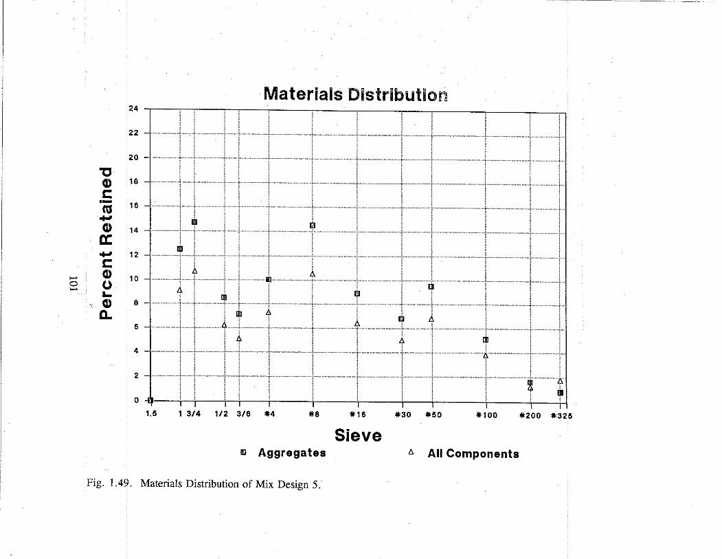
..... 0 .....

,, (I) c: ·-ca .... (I)

a: .... c: (I) (.) a.. (I) a.

_______ ,_ .. __ ,, _____ , ____ ,_ ___________ _

Materials Distribution 24 ,-~---,~,--~-,----,-~~,--~~-,-~~~,--~~---,-~~,--~~~~~~~~~...,,

22 - .......• ······: .............. ) ······: ...... .:... ·············: ·:········ .. ··········· .... : ............ ····i······ ··················· ···~ ··················:

I , 20 - ··················~ ······!······ ······f ······! ................ ; .......... ··············] ···1 ··+·· ............. ! ······················· ·····~··········· .............. i

1 ........ l. . .. !... ········: ..................... ·······!············· ············1 .. , ........ L .... ···········l··· ···1 ................ '.. 18 -

16 -· ............... , ...... , ............... , ...... , ........................................ , ........................ , .... ..

......

·.·.·.• ••• ·· ···············: ......................................... ···············i ............... l .. .

, I r 14 - ................. : ... ill l. .... ijJ

12 -

10 -

8 -

6 -

f:, ...... , ...... i 4 ' l ...... i ...... !

.............. : ........................... .j. ............................................... ) '

4 ........................... ! ....... !···············-......... j·····

ijJ ''iii

......... ! ...... ,

' mil .......... ! ..... ·i ................ ,. .. . .......... ····· ...... ~

4 ................ ; ......................... ; ................ i. ' .. ..... j

: , A····~ + ' 4 ~ f:, .......... -r·· :

......... ···~ ............. ;

........ 1 ............... : ...

............ ! .......... j ...

4 -······· • • •. • .. . • ! :r: . J: ·· ·· I : ' ............... : T ! ............... ; ··~ I 2 -

~ '{!.' . ........ i ············· .. :···

0 -111-~--r,~f--,~~,,.--;--,~~,,.--~~~,r-~~-;--,~~-;--,~-r-,~~~~,~~~~,~~T-1,

1.5 1 3/4 1/2 3/8 #4 #8 #16 #30 #50 #100 #200 #325

Sieve 111 Aggregates l!. All Components


CHAPTER 2: FIELD TEST IN LA PORTE

2.1. INTRODUCTION

The test sections on SH 225 in La Porte, Texas, were paved on November 11, 1991

and opened to traffic on December 12, 1991. These test sections are new CRC pavement

placed 13 inches (330 mm) thick with two layers of steel reinforcement. The total length of ·

the test pavement was 2550 feet (777 m) (Fig. 2.1) and was sub-divided into nine test sub

sections (with a buffer section at each end). Each sub-section was 250 feet (76 m) long, 12

feet (3.66 m) wide and each buffer section, 150 feet (45. 7 m) long. Paving started at the

west end of the test pavement at 8:00 a.m. and ended at the east end of the test pavement at

8:30 p. m. The paving direction was identical with the traffic direction. Although the

concrete mix design was the same for each sub-section pavement of the test, different

orientations of the transverse steel reinforcing, different curing methods and different

cracking control methods were applied. The purpose of the field investigation was to detect

the factors that affect the cracking behavior of the CRC pavement. Many different variables

were measured and cracks were surveyed at pavement ages ranging from 3 days to 125 days.

2.2. STEEL REINFORCEMENT AND CURING METIIODS

The concrete used for the pavement contained river gravel as the coarse aggregate.

The pavement section had two layers of reinforced steel with #5 steel as the longitudinal

rebars and #6 steel as the transverse rebars. The top layer of transverse rebars was placed at

the mid-depth of the pavement; and the bottom layer of transverse rebars was 2.5 inches

(63.5 mm) above the surface of the subgrade (Fig. 2.2). In all the sub-sections except Sub

section 2, the transverse rebars were perpendicular to the longitudinal reinforcement, and the

interval between adjacent longitudinal rebars was 8 inches (203 mm) while adjacent

transverse rebars were placed 3 feet (0.91 m) on center. Accordingly, the percentage of the

longitudinal steel was 0.6%. The transverse reinforcement was placed in an alternating

pattern between the fop arid bottom fa)'ers offongltudinal steel as shown in Fig. 2.2.

103

--- ·-·-----··-----

North

Q) '--:::i ()

Q) -0 '--..... al

'-- ~ -0 Q)

:t= () c 0 al :::i '-- ..... en Q_ Cf)

0 1 2

10 ~ c 0

15 0

3

Skewed Transverse

Steel

Q) '--:::i Q)

() c Q)

-0 £ '--al -0 .....

Q) c >-al 0 .....

Cf) Q_

4 5

Q) Q) Q) '-- '-- '--:::i :::i Q) ::'.:! () () c 0 Q) -0 -0 >- -0 '-- '-- '--,al (\j .c (1l -0 -0 ..... -0 '--Q) Q) c c >- c :t= (\j al 0 ,£1! ..... - :::i Cf) Cf) Q_ Cf) en

6 7 8 9 10

Sawcut Sawcut

45.7 m 76.2 m 76.2 m 76.2 m 76.2 m 76.2 m 76.2 rn 76.2 m 76.2 rn 76.2 rn 45.7 (150') I (250') I (250') 1 (250') 1 (250') I (250') 1 (250') 1 (250') 1 (250') 1 (250') 1 (150')

777 m (2550')

Fig. 2.1. Layout of the Test Sections in La Porte, Texas.·

33cm

(13")

Longitudinal Steel Rebar

><+r <s•·•·••••···••··••••••••• .. ••.s•····t·•·<·••·•··1·•••R>b•••••••·•·> ·····.·.·· .... 1 an verse . ee ...... e. ar .·.·.·.·.·.·.·.·.:-:.:-:-:-:-:-:-:.:.:-·.:····.

0.91 ri1 (3') 0.91 m (3') 0.91 m (3')

This sketch is not in proportion to the actual size.

Fig. 2.2. Steel Rebars in the Pavement of the Test Sections.

16.5 cm

(6.5")

6.5cm (2.5')

Transverse steel rebars were skewed in Sub-Section 2 to form an angle of 60° with the

pavement edge. These rebars were also placed 3 (0.91 m) feet on center. Four different

curing methods were employed. The curing method applied to each section is indicated in

Fig. 2.1. These curing methods are as follows:

(i) Membrane curing compound, Item 360.2 (13), is referred to as the

standard curing method and noted as "Standard Cure";

(ii) Membrane curing compound, Item 360.2 (13), using Procrete - a

proprietary product, is noted as "Procrete";

(iii) Cotton mat curing, Item 360.2 (15), plus membrane curing, Item

360.2 (13), noted as "Cotton Mat"; and

(iv) Polyethylene film curing, Item 360.2 (12), plus membrane curing,

Item 360.2 (13), noted as "Polyethylene."

The buffer sections were cured with the standard curing methods.

2.3. Sawcut for Crack Control

The longitudinal joint in the test sections was cut by using early-aged sawcutting

techniques. This technique is different from conventional sawcut methods which use external

sources of water to cool the blade during cutting operations. This method allows the

concrete to be sawcut at an early age with minimal or no raveling which is typically much

earlier than what is possible using conventional sawcut methods. The notch placed by the

early-aged method was approximately 1 inch (25.4 mm) in depth.

The early-aged technique was used to place transverse sawcuts at specified intervals in

Sub-Sections 6 and 9. A series of transverse sawcuts 175 feet (53. 3 m) in length was placed

in Sub-Section 6. Within the series, the spacing of the transverse sawcuts was 3 feet for a

length of 57 feet, and in the remaining portion, the spacing of the transverse sawcuts was 5

feet (4.5 m). The transverse sawcut operations started at 9:00 p.m. on Nov. 11, or about

seven hours after placement of the concrete in Sub-Section 6. Four sawcut machines were

used simultaneously in order to meet the pavement cutting schedule. Sawcutting operations,

Sub-Section· 6, ended at 9:00 ·a.m., November 12. NOil.pparerifril.vellirigoftliesawcufJofriis

was evident. Twenty-five feet of Sub- Section 9 was sawcut transversely.

106.

--------·--·--- ··------·--·· ·--- ------

2.4. Weather Information

A portable weather station was placed near the test sections during and after

placement of the concrete, recording the ambient temperature and relative humidity at the

time of paving. Fig. 2.3 shows hourly temperature data acquired once an hour from

November 11 to November 16, 1991. The origin of the time scale in the figure indicates

0:00 a.m., November 11. The relative humidity data represent instantly recorded data while

the temperature data represent an average over an hour. As seen in the figure, the daily

average temperature rose over the three-day period as did the daily average relative

humidity.

2.5. Measurement of Pavement Temperature and Relative Humidity

Temperature and relative humidity are two important variables for concrete. Changes

in either of these conditions can induce stresses in the pavement as well as affect the rate of

the strength gain of the concrete. The influence of the parameters is very apparent during

the early ages of the concrete .. Both temperature and relative humidity in the test sub

sections were measured with two different digital systems. One was a product of Vaisala, in

which the sensor is a capacitor. It monitors the change in capacitance of a thin polymer film

as it absorbs water vapor. The other, manufactured by General Eastern, measures the

change in electric resistance of a bulk polymer sensor with the moisture the sensor absorbs.

To implement these instruments, a PVC tube was inserted in the pavement from the

pavement top surface. The lateral wall of the tube was tightly fitted into the pavement

concrete and the concrete was exposed to the sensor though the opening end of the tube (Fig.

2.4). When the temperature and relative humidity were measured, the probe of the

measuring system was inserted in the PVC tube with a rubber seal fastened around it to form

a small closed space between the sensor unit and the concrete. After the measurement, the

probe was removed and a PVC cap was placed on the top end of the tube to prevent air

exchange between the space inside the tube and the atmosphere.

For each sub-section, 1 and 112 inch (25 or 13 mm) deep holes were formed in the

pavement surface where the probe was inserted. Therefore, the temperature and relative

humidity measurements were for the concrete close to the pavement top surface. Where

107

..... 0 00

~

u ~ .. .. " -" .. .. .. s " ....

TEMPERATURE & RELATIVE HUMIDITY VS TIME La Porte, Texas

26 ;.,--------------------------r-120

24

100 22

20 rl; • I!' 80

18 ' \ Iii .. '

16 : • 60 ' '

14 ' ' ; • 40

12 ;

~ 10 ~ '

.. i 20

8 .. 6 -1-----~---~----~---~---~-----+-0

0 24 48 72

Time (hours) 96

\-•- Temperature ""*- Relative humidity I

120 144

Fig. Ambient Temperature and Relative Humidity Records.

~

* ~ .€' .... ·a " ::i:: .. ~ ·.:: .:: ... >.::

Digital Display

Seal

/General Eastern Meter

/PVC Tube

Sensor . . . . . . . . . . . . .... ·.·.·.·.·.· ..... :-:-:-:-:-:-:-:.:-:.:1

:\'. : • : :: . : ::: :-:: : : . : :.~ \ ·.• ·.: .• ··.~ .•. ~ ·.: ·.·.,-.~ .•. ~ :.~ .~.· .• .~.· .•... ~ . ·.~.· .• ·.~.· . ·.~.· .: '.~.-.• ::::::··-·;·.·.·.·:::;:::::··:··-·.·.·.·

:~::~:::;\;:;:;~~~~:::::;:::::::~:~:~::;~;;~;~;:::::::~:~::::~::::::::~ . . . . . . . . . . . . . . . . . . . . . . . . . . . . . . : :: : : : ~

:~;~~~~~:~ i ~ i ~ (~~; ~; { ~ i: { ( ;~ \~ \ ~ { ~: ~ ~: ~: ~:~} ~:~:~: ~~ ~: i ......_ _ __.4 .·.·.·.·.·.:.:··-·.·.·-:-:-:-·-·.·.·.

Fig. 2.4. A Set-Up for Measurement of Temperature and Relative Humidity in the Pavement.

109

these measurements were made automatically by a portable data recording system, the data

were downloaded from the data logger system for analysis. In this way, continuous

recording was achieved. Three channels in the data logger (with one probe per channel)

were used to record the temperature and relative humidity at three different depths in the

pavement: 1 inch (25.4 mm), 2 inches (50.8 mm) and 4 inches (101.6 mm). For security

reasons, the logger system had to be dismantled during off hours, which meant that data

during these periods of time were not recorded. The digital records and the graphs are

included in Appendix I. As shown in the graphs, a period of time is necessary to achieve a

stable record of the relative humidity. The readings over 100% were caused by saturation of

the sensor element and should be considered showing 100% relative humidity in the closed

space. Two of the three channels had good calibration for temperature measurement. The

other one must be calibrated such that the reading can be interpreted properly.

Changes in the temperature and relative humidity in each test section measured are

shown in Figs. 2.5 to 2.13, one figure for each section. The starting time of paving for each

section is shown in the caption of the figure.

For comparison of different curing methods, temperature and relative humidity data

for Sub-Sections 1, 3, 5 and 6 are shown in Figs. 2.14 and 2.15. The curing method used in

each of these sections is indicated in the figures. It is speculated that the cotton mat kept the

pavement from solar radiation, and, as a result the temperature in Sub-Section 3 was lower

than in other sections (Fig. 2.14). The polyethylene film covering the pavement (Sub

section 5) caused a "greenhouse" effect, which made the temperature in Sub-Section 5 higher

than that in sub-sections which used other curing.methods. However, change in temperature

of pavement was caused by complicated environmental conditions as well as properties of

concrete mix. Further observations are necessary before a conclusion may be reached. On

the other hand, the relative humidity in Sub-Section 5 was the highest (Fig. 2.15), since the

polyethylene film isolated the pavement top surface from the atmosphere and kept the

moisture in the pavement from evaporating. Between the two membrane curing methods, the

standard method (Item 360) caused a lower temperature and higher relative humidity in the

pavement than the proprietary product.

110

____ _,__ _ _________ . _____ ,. ___ _-_ _,_·~-

100- Ill Ill Ill Ill

- Ill Ill

......... 80- Ill '# ----->. 0 -

:t::: ..._...

"O ~ 60-E :J :J rtl -..... I ._ ..... Q) ..... Q) C...40-.> E rtl Q) -

!'. I- !'. Q) !'. !'. !'.

a: 20- !'.

-Section 1, La Porte I Ill R.H. "'Temp.

0 ' I I I I ' ' ' I I ' 0 2 4 6 8 10 12

Time (day)

Fig. 2.5. Temperature and Relative Humidity Records for Section 1.

100- + + +

+ + + - + - 80-?ft.

...__.. ->-0 -~ ..._... ""O ~ 60-E ::J

+" ::J ct! -- I L. - (])

I'-> (]) 0..40-.> E +" ct! (]) - x x (]) I- Xx x

a: 20- x x

-Section 2, La Porte + R.H. x Temp.

0 I I I I ' I ' ' . ' ' I

0 2 4 6 8 10 12

Time (day)


100 () <>

()

<> <> <>

<>

........... 80 cf, <>

................... >. 0

:!:: ........ "O ~ 60 E :J ..... :J Ctl I .._ - Q.) - Q.) C..40 w

.> E ..... Ctl Q.) \1

I- \1 \1 Q.) \1

a: 20 \1 v

Section 3, La Porte <> R.H. "Temp. 0

0 2 4 6 8 10 12

Time (day)


100- Ill Ill

Ill -

Ill .-... 80-Cf.. ..._... .........

£2. -

"O ~ 60-·-E ::J +-' ::J ctl -- I ..... - Q) ...

Q) 0.40-> E :.;::::; ctl Q) - A

Q) f- A A

A A a: 20- A

-Section 4, La Porte 111 R.H. A Temp.

0 I I ' I I I l I I -, l

0 2 4 6 8 10 12

Time (day)


100 + + + +

+ +

.......... + '#- 80 -->.0 :!::::! ..._... "O ~ 60 ·-E ::J

+"" ::J ctl - I ..... - Q)

Vi Q) 0..40 .> E +"" Q) x x ctl x x Q) I- x x x a: 20

Section 5, La Porte + R.H. x Temp.

0 0 2 4 6 8 10 12

Time (day)


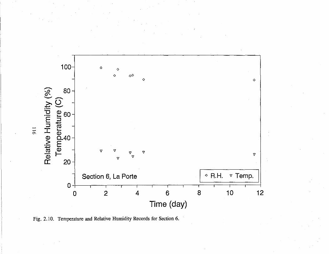
100- 0

0 oO - 0 0

............ 80-(fl. -->.0 :t: ..._.... -

"O ~ 60-·-E :J :J 1i1 -- I - ....

°' Q) Q) 0..40-> E +:i ro Q) - "' I- "' "' Q)

"' "' a: 20-

- Section 6, La Porte 0 R.H. "' Temp. 0 I I I I ' ' ' ' I I

0 2 4 6 8 10 12

Time (day)


100- llll Ill Ill II

ill ill -

- 80-(fl. -->.0 -:!::: ......... "C e 60-E ::J ::J 10 -I ..... - Q) - Q) C...40--..]

> E 1o Q) - A I- A A

Q) A A

0: 20-

-Section 7, La Porte 1111 R.H. "Temp.

0 I I I I I I I I I I I

0 2 4 6 8 10 12

Time (day)


100 + + +

+ - 80 *' ---- ->.0 :t= .............. "'O ~ 60 E ::J ........ ::J ro - I ._ - Q)

00 Q) C..40 .> E x ........ x ro Q)

Q) I- x x

a: 20

Section 8, La Porte + R.H. x Temp.

0 0 2 4 6 8 10 12

Time (day)


100- 0 0 0

0 -

<> 0

......... 0

Cf.. 80-................... >.0 -

.:t::: ...._.... "O ~ 60-E :J :J rti -

~ I ...... ~ Q) \0

Q) 0..40-.> E rti Q) - '\!

I- '\! 'V Q)

'V 'V a: 20-

-Section 9, La Porte o R.H. v Temp.

0 I ' I I I I ' ' I I I

0 2 4 6 8 10 12

Time (day)


Temperature (C) SH 225, La Porte, Texas 35 .--~~~~~~~~~~~~~~~~~~~~~~~~~~~~~~----.

30

25

20

15.

10

5

0 12/11/91 13/11/91

Procrete Section 1

14/11/91 15/11/91

Recording Date

raining

19/11/91

Cotton Mat 1m:mm1 Polyethylene D standard Section 3 i!in;:; Section 5 Section 6

Fig. 2.14. Temperature Change in Sections Cured with Different Methods.

22/11/91

R.H.(%) SH 225, La Porte, Texas (paved 11111/91) 120 .----~~~~~~~~~~~~~~~~~~~~~~~~~~~~~~~--.

100

80

60

40

20

0 12/11/91

(4:00 pm)

II

13/11/91 (6:30 pm)

Procrete Section 1

14/11/91 (5:30 pm)

15/11/91 (10:00 am)

raining

19/11/91 (9:00 pm)

cott~n Mat 1mrnmrn1 Poly~thylene D standard Section 3 ;;;;;;;;;;;; Section 5 Section 6

Fig. 2.15. Relative Humidity Change in Sections Cured with Different Methods.

22/11/91 (2:00 pm)

2.6. Measurement of Pulse Velocity of Pavement

The basic principle upon which the pulse velocity method is founded proposes that if

the velocity of a pulse of longitudinal waves through a medium can be determined, and if the

density and the Poisson's ratio of the medium is known, then the dynamic modulus of

elasticity of the medium can be computed. Furthermore, knowing the dynamic modulus of

elasticity, other mechanical properties can be estimated from empirical correlation with it.

Pulse velocity measurements in each section were made in conjunction with

temperature and relative humidity readings, because previous research indicated that

temperature and moisture conditions of the concrete had insignificant effects on the pulse

velocity. Accordingly, the pulse velocity could be considered an independent parameter to

estimate the concrete strength. It was also of interest to examine the possibility of

determining the proper time of sawcutting based on pulse velocity readings.

The V-Meter, a portable ultrasonic testing unit, was borrowed from the Federal

Highway Administration (FHWA) in Washington, D.C. and used in every test sub-section to

measure the pulse velocity. The V-Meter uses two transducers, one each for transmitting

and receiving the ultrasonic pulse. The pulse travel time is displayed in three numerical

digits ranging from 0.1 to 999 microseconds. In the sub-sections, the two transducers were

placed on the pavement top surface, 12 inches (304.8 mm) apart from each other. Grease

was used to improve the contact between the transducer end surface and the pavement

surface. The measured ultrasonic velocities for each test section are shown in Figs. 2.16 to

2.18. For digital data, see Appendix II.

Since there was reinforcing steel in the pavement, a question may exist if the effect of

the rebar on the pulse traveling time is negligible. Analysis results indicate that the effect of

the rebar can be ignored when the rebar is embedded deeper than half the distance between

the transducers, which is the case of the measurements performed in the sub-sections. For

further discussion, see Appendix III. Therefore, the pulse velocity was simply obtained by

dividing the distance between the two transducers, 12 inches (304. 8 mm), by the recorded

pulse traveling time, and then multiplied by a factor 1.05. The factor 1.05 was a

122

4000 <>

~ Bl ' + + !?Ill Ill . - + + (.) Q)

~ Ill +

E 3000 <> .._... >- <>

:t:: <> (.) Ill

0 ..... Q) <> N <> w > Iii

Q) 2000 (/)

:J 0....

D Section 1 + Section 2 <> Section 3

0 2 4 6 8 10 12

Time (day) Fig. 2.16. The Pulse Velocity in Sections 1 to 3.

-(.) CD (/) -E 3000

Ill -->-:t= (.)

- 0 N CD .j>.

> CD 2000 (/)

::J 0..

~

Ill

<)

'V

'V

<)

'V

11'.l

111 Section 4 "' Section 5 <> Section 6

~

1000-+--~.----,~~~~~-.--~~--,--~~~--.-~.----,~-1

0 2 4 6 8 10 12

Time (day) Fig. 2.17. The Pulse Velocity in Sections 4 to 6.

4000 <>

!J 'V lZ >«

......... ~

() Q)

~ <>!iii E 3000 <> - x x

>. 'V :!::::: () 0

- Q) N > Vl

Q) 2000 U'J :J a..

Section 7 <>

'V Section 8 x Section 9

1000 o 2 4 6 8 10 12

Time (day)

Fig. 2.18. The Pulse Velocity in Sections 7 to 9.

compensation for the pulse travelling distance since the pulse path was not along a straight

line.

From the V-meter measuring records on test sections 5 and 6, an increase in pulse

velocity with the pavement age can be expressed as with the coefficient of correlation r2 =

0. 715 (Fig. 2.19):

[ PV ) = 7.80 (Age)°-306

1000

where PV is the pulse velocity in feet/sec and Age is the pavement age in days.

(2.1)

Since the pulse velocity was not measured as early as the sawcutting started in the test

s_ections, the above equation would be extrapolated to estimate the pulse velocity in the

pavement when the sawcutting started. As reported above, the sawcutting started 7 hours

after paving for Sub-Section 6. The pulse velocity then is given by Eq. (2.1) as PV = 5350

feet/sec (1630 m/sec). As the Concrete Technology Laboratories, Inc. (CTL) reported, the

pulse velocity of the concrete that used 500 lb/yd3 (2.12 MN/m3) of cement in the mix design

with the rounded gravel as the coarse aggregate was 5800 ft/sec (1800 m/sec) at 9-hour age

when curing temperature was 50°F (l0°C). This confirms the conclusion drawn by the field

test as part of the same research project, Project 1244, on the test sections in Texarkana,

Texas. The test sections in Texarkana were jointed concrete pavement, placed in October

and November 1991, where the pulse velocity was measured when the joints were sawcut. It

was reported that, in Texarkana, no apparent ravelling occurred when the pulse velocity had

increased to 3600 - 4600 feet/sec (1100 - 1400 m/sec). These results suggest that the

pulse velocity may be used for determining the proper time for sawcutting.

2. 7. Measurement of Compressive Strength of Concrete

Two batches of standard-sized concrete cylinders were cast in the field. The first set

was prepared at 1:00 p.m. when Sub-Section 5 was paved. The second set was prepared at

5:00 p.m. when test section 9 was paved. These specimens were tested in compression at

concrete ages ranging approximately from 12 hours to seven days. The test data are

126

- Ill (..) 3000 + Q) +

~ Ill E _. +

>. Ill

:!:::: 2000 (..)

- a N Q) -:i

> Q) (/)

1000 ::J 0... {> Test Section 5

Ill Test Section 6

0 0 1 2 3 4 5

Age (days)

Fig. 2.19. Change in the Pulse Velocity with Pavement Age.

included in Appendix IV and shown in Fig. 2.20, where regression of the data on a semi

logarithmic curve is

Age = 0.534 + 2.613x 10-4 (f:) +1.901 x(l0f7 (()

2 (2.2)

where f{ is the compressive strength in psi and Age is the concrete age in days. The

coefficient of correlation r2 is 0.956. From this regression and relationship between the

pulse velocity and the concrete age, correlation of the pulse velocity with the compressive

strength is obtained, which is shown in Fig. 2.21. The regression curve for the correlation

is included in the figure as well. The regression equation is as follows:

[ PV ] = 0. 724 (f1)°"340

1000 '

where PV is the pulse velocity in feet/ sec, and f~ is the compressive strength in psi. The

coefficient of correlation r2 is 0.694; According to previous work by Construction

Technology Laboratories, Inc. (CTL), the relationship between the pulse velocity and the

compressive strength can be expressed as:

log f: = 0.732 + 0.192 PV 1000

(2.3)

(2.4)

This curve is shown in Fig. 2.21, noted as CTL. From the same value of the pulse velocity,

the CTL curve predicts lower compressive strength. It is worthwhile to point out that CTL

curve was obtained based on the laboratory specimens while readings taken for the pulse

velocity in this study were taken on actual pavements.

2.8 Measurement of Fracture Toughness

Four beam bending specimens were prepared in the field along with the first set of

cylinder specimens. These specimens were of the same shape (Fig. 2.22). The depth of

128

40 m -CC! a..

~ 30 ----.c

+-' O') c Q) Ill ,_

+-' Ill (f) 20

>-' Q) N .> l.O

Cl) Cl) Ill Q) ,_ a. 10 E

Ill Specimens were prepared in situ 0 0 during placement of test section 5

and the west buffer section. 0

0 2 4 6 8

Age (days)

Fig. 2.20. Change in the Compressive Strength with Concrete Age.

-.. (.) Q)

.s!2. E .....,. >-~ (.)

- 0 w

Q) 0

> Q) (/)

:J 0..

4000

3000

2000

1000

0

• • • • ' ' ' •

'

• •

CTL - .. -- --.. ---· -- . --Lab data .... ---.........

Pulse velocity of the pavement measured in situ

.... - ..

Ill

---_ .. -- .. __ ......... .. ---.. ----

Ill 6

---- --_ ......

6 Test Section 5

w Test Section 6

4 8 12 16 20 24

Compressive Strength (MPa)

Fig. 2.21. The Pulse Velocity versus the Compressive Strength.

--- --

28

Fig. 2.22. Notched Beam Specimen.

. p

. . . . .

. . . . . .

0 ..

s

d

the specimens was 4.5 inches (114 mm), 6 inches 152 mm), 9 inches (229 mm) and 12

inches (305 mm), respectively. The support span of the beam specimen was 2.5 times the

depth of the specimen. A notch was cut by a saw before testing. The length of the notch

was a quarter of the beam depth. The width of notch was about 1/8 inch (3.2 mm). Three

point bending tests were performed on these specimens two days after preparation of the

specimens. The load was placed on the other side of the beam specimen rather than the

notched side. Two fracture parameters were calculated from the peak loads of the four tests

based on the size effect law (SEL). For a brief review of this theory and the test method,

see Chapter 4. Fig. 2.23, shows the test data and a regression line. The parameters

obtained are:

Klf = 987 psi.Vin = 1.08 MPaVm, and cf = 2.23 inches (56.6 mm),

where K1f is the critical stress intensity factor for an infinite specimen and cf is the effective

critical crack increase for an infinite specimen, as defined in the size effect law. These are

both material parameters which can serve as indicators of the crack susceptibility of the

concrete.

2.9 Correlation of Fracture Toughness with Compressive Strength

From the laboratory fracture tests and compressive tests on concrete using river

gravel as the coarse aggregate, Klf increases with the age ranging from 12 hours to 28 days

following an equation as:

[ Kif ] = •rxge K~s J 28

(2.5)

where Ki8 is the Kif value at the 28-day age (See Chapter 4). This curve does not fit the data

for the 12 hour and twenty-eight day ages well, but shows the trend of increase in K 1f with

the age of concrete. By assuming a linear relationship, the following equation is obtained for

change in Kif during the first day:

Klf = 1.333 [Age] - 0.333 K~ 1

(2.6)

132

--------- ---

N

m 0.. .:.:: ........ .... -~

w N w 15:" ........ 'O .0 -

0.05,.-----~-------~----....,,___-~

0.045 •

• 0.04

• 0.035

0.03 •

0.025

0.02•-+------~----~-----~-------'

0 10 20 d (cm)

30 40

Fig. 2.23. Fracture Test Data and the Regression.

where K/t is the Krr value at the one-day age (Fig. 24). According to this equation, Krr

remains zero for a couple of hours after specimen casting. This may be reasonable since the

concrete needs some time to take on a set. Also, compressive strength cannot be measured

before concrete has taken on a set. By combining Eqs. (2.1) and (2.6), Krr increase can be

related to the compressive strength. For a more accurate correlation for the age within the

first day, change in the compressive strength with time may be obtained:

f: = 1625 Age - 705 (2.7)

where f; is in unit of psi. Consequently, Krr may be expressed in terms of the compressive

strength as:

K rr = 0.818x10-4( + 0.244 1

Kif

where f; is in unit of psi.

2.10. Crack Surveys

(2.8)

Cracks in the pavement of the test sections were surveyed. Sub-Sections 6, which

was transversely sawcut after paving, was surveyed on November 14 (3 days after paving),

November 15 (4 days after paving), November 19 (8 days after paving), November 22 (11

days after paving), and November 26 (15 days after paving) in 1991. It was surveyed again

on March 16, 1992 (125 days after paving). Other sub-sections were surveyed 3, 15 and 125

days after paving. All the sections were opened to traffic on December 12, 1992.

In Sub-Section 6, most of the cracks were initiated from the sawcuts, but in other

sections, many cracks were initiated from the steel rebars. Fig. 2.25 is a sketch of the

view of the pavement edge. Many of these cracks initiated from the steel rebars finally

developed and moved completely through the pavement (Fig. 2.26). Table 2.1 shows the

increase in the number of cracks that were through to the pavement top surface (called

"surface cracks" for brevity) of each section at the 3-, 15- and 125-day ages of the

134

------ - ·- ---------------

0.8

0.6

0.4

0.2

0 0.2 0.4 0.6 0.8 1

Age (Days)

Fig. 2.24. Increase in Krr Value with the Concrete Age within One Day.

~ (~ I Ill i ~

@ (! ~ ~

Fig. 2.25. Cracking Patterns on the Pavement Edge. ·

• • • • • •

Fig. 2.26. Cracks Initiated from the Transverse Steel Rebars.

pavement, where Section 0 designates the buffer section at the east end, and Section 10, the

buffer section at the west end. The first column lists the number of the surface cracks

observed on the 3rd day and the second column shows the number of the surface cracks

formed between the 3rd day and the 15th day. In the survey of the 15th day, cracks that had

been initiated on the pavement edge but had not yet developed as surface cracks were

carefully investigated and recorded. It was found in the survey of the 125th day, that some

of the surface cracks formed between the 15th day and the 125th day were from these edge

cracks observed on the 15th day, and the rest of the surface cracks were "newly" initiated.

The numbers of these two categories of cracks, initiated before and after the 15th day, are

listed in the table. The last column of the table gives the total number of surface cracks that

existed on the 125th day. Since the shoulder had been built up with Sub-Sections 9 and 10 at

15th day, pavement edge of these two sections could not be seen then. The shoulder had

been built up along with every section on the 125th day, and therefore, cracks distributed on

the pavement edge of all the sections could not be seen on that date.

Table 2.1. Surface Crack Development with Time.

New Cracks @ Day New Cracks@

Section New Cracks New Cracks 141 Initiated Before Day 141 Initiated Total Cracks

No @Day3 @Day 15 Day 15 After Day 15 @Day 141

0 11 0 10 4 25

1 21 0 17 12 50

2 24 0 11 7 42

3 18 6 13 16 53

4 21 5 26 6 58

5 24 2 5 18 49

6 13 18 0 4 35

7 24 0 0 27 51

8 31 1 1 11 44

9 25 3 3 12 43

10 11 2 1 8 22

138

To exhibit the increase in the number of the surface cracks, Fig. 2.27 shows a bar

chart. Sub-Sections 0 and 10 (the west and east buffer sections) had fewer cracks than other

sub-sections (they were shorter). Among Sub-Sections 1 to 9, Sub-Section 6 had the fewest

surface cracks at the 3rd day and 15th day, obviously because the sawcuts controlled

cracking. The number of surface cracks of Sub-Section 6 at the 125th day was somewhat

uncertain since the edge had been covered by the shoulder and surface cracks newly initiated

from the sawcuts, if any, were unable to be recognized. From the number of surface cracks,

the average surface crack spacing was calculated. Change in the spacing with time is shown

in Fig. 2.28 for Sub-Sections 0 to 5, and in Fig. 2.29 for Sub-Sections 7 to 10.

Sub-Section 6 has been surveyed more frequently than other sections. Fig. 2.30

shows the records of numbers of surface cracks in the sawcut part of the section. Although a

part of test section 9 was transversely sawcut also, crack development in this part was not

investigated in detail because this part was much shorter than the sawcut part of Sub-Section

6. Change in the average surface crack spacing with time for the sawcut part of Sub-Section

6 is shown in Fig. 2. 31. Since it is not certain whether any surface cracks from the sawcuts

were formed between the 15th day and 125th day, the average spacing at the 125th day is not

included in Fig. 2.31. Two new surface cracks were observed at the 125th day, and it was

identified that they were both located over transverse steel rebars, though all the rebars could

not have been seen since the shoulder had been placed and covered the pavement edge.

However, all the surface cracks observed were either from the sawcuts or from the

transverse steel rebars. All the surface cracks in this part were initiated from weak points in

the pavement, the pavement sawcuts or interfaces between rebars and mortar. In other

words, no random surface cracks were observed in the sawcut part of Sub-Section 6.

From the change in the average crack spacing for all the sections but Sub-Section 6 (Figs.

2.28 and 2.29), it is seen that the number of the surface cracks increased rapidly within the

first three days, and the rate of the increase in number of surface cracks decreased with time.

Many sections did not have new surface cracks between the 3rd day and 125th day.

Among the four different curing methods, cotton mat and polyethylene reduced

temperature variation in the pavement and slowed down the concrete drying process, as

139

~ 40 ····························· e u ~ 30 ··-···························· t

,.Q

:j;"'. 8 0 i 20 ··························

10 ······················

0-1---0 1 2 3 4 5 6 7 8 9 10

Section Number

I • 3 days CIJ 15 days ~ 125 days

Fig. 2.27. Number ()f Surface Cracks of Each Section Observed on Different Dates.

-E -Ol c ·o Cll a.

Cf) - .::.::. .j:>. - 0 e! 0 Q) Ol e! Q)

~

4.5 ······························································· ..... ······· ........ .

4 ······················································ ························ ..................... .

3 ··············································

2 ..................... ························

1.5 ···················-·- .. ························ ········ ··········· ....... ... . .................. ·······················

1 ·················· .... ··················· ...... . . ..... ·················· .. .

0.5 ··············· ························································· ··············· ········································

01+-~.--.-.-..-.-n-.-~.-.-..-r-,-,...rn-~--r--.--r..:.,-,--.-r~

-Section O

-·-+-·· Section 1 -Section 2 -a

Section 3

-*Section 4

1 10 100 1000 Time (day)

Fig. 2.28. Change in the Average Surface Crack Spacing with Time for Sub-Sections 0 to 4.

-E -O> c: ·5 <ll 0..

Cl) .:.:: ...... 0 -!>-~ N () Q)

~ Q)

~

4.5 ················································································· ······································· ······················

4 ........................ ................... .......... ...... ......... . ............. .

3.5 ......... ······························ ........... .

3 ···············

1.5 ...... ······································· ···················

1 ........................... . ················· . . ....... ...... .......... . .. .

o+-~.--,--,--rnrn-r-~,-,--,-,.,,TTT~--Y~,-,-,rnrn

-Section 5 -Section 7 --a

Section 8

-x-Section 9

-.Section 10

1 10 100 1000 Time (day)

Fig. 2.29. Change in the Average Surface Crack Spacing with Time for Sub-Sections 5 and 7 to 10.

Cl) .:.:: (,) CIS ... 0 -0 ... Cl) .Q - E .j:o.

- w ::I z

18.00-,----------~~-~

1 6. 00 ---------------------------------------------------------------------------------

14. 0 0 ----------------------------------------------------------- ----------------------

12. 00 -----------------------------------------------------------

1 0. 00 -------------------------------------

8. 00 ---------------

6. 00 ---------------

4. 00 --------------

2. 00 --------------

0. 00-+----3 4 8

Time (day) 11

., Initiated at Notch ~ Initiated at Steel

15

Fig. 2.30. Change in the Number of Surface Cracks with Time for the Sawcut Part of Sub-Section 6.

9· .............................................................. ·········································· ...

-E 8- ................................................................ ········ ·········· ....... .... . ............... . ... -

Cl 7· ···························································································· c: ·o <U a.

6· ....... ......... ................... ..... . ...................... . (/)

.:::t:. - 0

""" !!! """ ()

Q)

5- ......... ································ .... ..... .. .. ..... ...... ........ .. ... ......... ..

4 ........................................................................ .

~ ~

3· ....... ··································· ............ :...:·· .. ······ .... .

2······································ .............. ~ .................... .

1 · ....... ············ ............. ·········· ........ .... ...... ····· . .

01+-~~.-,~,~~,,~~,~,~,~~-~,-.-,~,-~,,-~,~,~,~,~-,.,~~,,.--,.......,,,~-.-r,,~,--M,

1 10 100 1000

Time (day)

Fig. 2.31. Change in the Average Surface Crack Spacing with Time for the Sawcut Part of Sub-Section 6.

displayed in the section titled "Measurement of Pavement Temperature and Relative

Humidity." As a result, increase in the number of surface cracks in Sub-Sections 3, 5 and 8

was suppressed in the first three days, but more surface cracks were formed between the 3rd

day and 15th day (Cotton Mat and Polyethylene were removed 7 days after paving). It

appears that the formation of these surface cracks were delayed by the effect of these two

curing methods.

Data listed in Table 2.2 are the results of the survey conducted on the 15th day,

which indicates that cracks were mostly initiated from the interfaces of the steel rebar and

mortar or the sawcut tips, because of the stress concentration at these locations, where

structure geometry, and/or material properties changed sharply. Fig. 2.32 shows the number

of surface cracks at the 15th day for each sub-section and the number of surface cracks that

were initiated from the steel rebars. Besides surface cracks, or cracks that went through the

top surface of the pavement, there were many cracks observable on the edge surface of the

pavement, which would potentially develop to form new surface cracks (Fig. 2.33). These

cracks, which were observed on the pavement edge but did not extend to the pavement

surface, are called "edge cracks" for brevity. Except for Sub-Section 6 and Sub

Table 2.2. Crack Survey Results on Day 15.

Section Number 0 1 2 3 4 5

No. of Surface Cracks 11 21 24 24 26 26

No. of Surface Cracks 7 17 11 18 21 26 Initiated at Steel .

No. of Edge Cracks not 19 46 18 7 21 3 Developed to Surface Cracks

No. of Edge Cracks Not 16 43 12 2 16 3 Developed to Surface Cracks,

and Initiated at Steel

Total No. of Surface & Edge 30 67 42 31 47 29 Cracks

Percentage of Cracks Initiated 77 90 55 65 79 100 at Steel

145

CJ) 30 ··················-····························································································································

~

~ 25 : ................................................... .

(.)

~ 20 ··········································· I-...... 0

""'" 0\ .... 15 ···········································

Q) .0 E 10 ...................... . ::J z 5 ...................... .

O-¥=== 0 1 2 3 4 5 6 7 8 9 10

Test Section Number

J R Total Crack Ill Crack On Steel

Fig. 2.32. Number of Surface Cracks for Each Section on the 15th Day.

~ (.)

~ 0 0 ._ al .0 E :::l z

60

50

40

30

20

10

o..J.C:== 0 1 2 3 4

Test Section Number

[~Surface Cracks~ Edge Cracks

Fig. 2.33. Number of Surface Cracks and Edge Cracks for Sections 0 to 5 on the 15th Day.

5

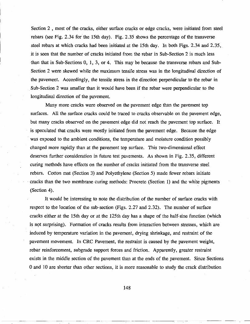
Section 2 , most of the cracks, either surface cra~ks or edge cracks, were initiated from steel

rebars (see Fig. 2.34 for the 15th day). Fig. 2.35 shows the percentage of the transverse

steel rebars at which cracks had been initiated at the 15th day. In both Figs. 2.34 and 2.35,

it is seen that the number of cracks initiated from the rebar in Sub-Section 2 is much less

than that in Sub-Sections 0, 1, 3, or 4. This may be because the transverse rebars and Sub

section 2 were skewed while the maximum tensile stress was in the longitudinal direction of

the pavement. Accordingly, the tensile stress in the direction perpendicular to the rebar in

Sub-Section 2 was smaller than it would have been if the rebar were perpendicular to the

longitudinal direction of the pavement.

Many more cracks were observed on the pavement edge than the pavement top

surfaces. All the surface cracks could be traced to cracks observable on the pavement edge,

but many cracks observed on the pavement edge did not reach the pavement top surface. It

is speculated that cracks were mostly initiated from the pavement edge. Because the edge

was exposed to the ambient conditions, the temperature and moisture condition possibly

changed more rapidly than at the pavement top surface. This two-dimensional effect

deserves further consideration in future test pavements. As shown in Fig. 2.35, different

curing methods have effects on the number of cracks initiated from the transverse steel

rebars. Cotton mat (Section 3) and Polyethylene (Section 5) made fewer rebars initiate

cracks than the two membrane curing methods: Procrete (Section 1) and the white pigments

(Section 4).

It would be interesting to note the distribution of the number of surface cracks with

respect to the location of the sub-section (Figs. 2.27 and 2.32). The number of surface

cracks either at the 15th day or at the 125th day has a shape of the half-sine function (which

is ngt surprising). Formation of cracks results from interaction between stresses, which are

induced by temperature variation in the pavement, drying shrinkage, and restraint of the

pavement movement. In CRC Pavement, the restraint is caused by the pavement weight,

rebar reinforcement, subgrade support forces and friction. Apparently, greater restraint

exists in the middle section of the pavement than at the ends of the pavement. Since Sections

0 and 10 are shorter than other sections, it is more reasonable to study the crack distribution

148

Q) Q) -CJ) Q)

~ Q)

> U) c: co ,_ I-c: 0 U) ~ - (.)

""' co "'

,_ 0 -c: Q) (.) ,_ Q)

Cl..

100~~~~~~~~~~~~..-~~~

90

80

70

60

50

40

30

20

10

.......................................................................

o-ic== 0 1 2 3 4

Test Section Number

j B Surface Cracks ~ Edge Cracks

5

Fig. 2.34. Percentages of Surface Cracks and Edge Cracks that Were Initiated at Transverse Steel Rebars in Sections 0 to 5 on the 15th Day

80

70

60

50 ..... c: w .....................

~ 40 w 0.

30

20

10

01-¥----0 1 2 3 4 5

Test Section Number

Fig. 2.35. Percentages of Transverse Steel Rebars that Initiated Cracks on the 15th Day.

in terms of number of surface cracks per unit length, which is called "crack density," instead

of the number of total cracks for each section. Distribution of the crack density on the 15th

day and the 125th day is shown in Figs. 2.36 and 2.37 respectively. A regression on the

half-sine function based on the least square method is given in each of the figures. In Fig.

2.36, the regression equation based on the least square method is:

r = 0.0599 + 0.511 sin?r(~) L

at the 15th day (2.9)

where ! is the crack density in number of surface cracks per foot and x designates the

distance from the west end of the pavement, and L is the total length of the pavement, or

2550 feet (777 m). (This length of pavement was placed in one day) The coefficient of

correlation r2 is 0.827. The regression with the least square method for the 125th-day data

is:

r = 0.167 + 0.034 sin7r(~) L

at the 125th day (2.10)

The coefficient of correlation r2 is 0.988: Crack densities for Sub-Sections 6, 8 and 9 at the

15th day (Fig. 2.36) are far apart from the regression, which was calculated from the data

for Sub-Sections 0, 1, 2, 4, 7 and 10. This may mean that sawcutting and polyethylene

curing caused higher crack densities than the other crack control and curing methods. Sub

section 3 was cured with cotton mat and had fewer cracks than the sub-sections cured by

membrane methods at the 3rd day, but its crack density at the 15th day had increased to be

close to the regression curve. Sub-Section 5 was cured with polyethylene. Although it did

not obtain an increase in the crack density as rapidly as Sub-Section 8, it did obtain a higher

crack density from the 3rd day to the 15th day. However, at the 125th day (Fig. 2.37), the

crack density for Sub-Section 6, and Sub-Sections 5 and 8 were lower than the regression,

which was calculated from the data for Sub-Sections 0, 1, 4, 7, 9 and 10. In other words,

these preliminary results indicate that sawcutting developed cracking in early ages but

reduced the crack density on a long-term basis. Besides Sub-Sections 5, 6 and 8,

151

........... E ~

0.4 Q)

..0 E 2

~ l!l ::s 0.3 1 3 c ...._.. D >- 0

:!::::: Ill ...... (/) Vi I'-> c 0.2

Q)

0 ~ (.) ctl 0.1 ...... 0

0 0.2 0.4

Fig. 2.36. Crack Density Distribution on the 15th Day.

5

x L

Ill

6

0.6

l!l 7

0 8

Ill

9

m 10

0.8 1

1

-- 0.9 E

--.:::-Q) 0.8 ..0 4 E llll

::::l c 0.7

1 ->- D 3 5 :t::: 0

..... en 0.6 8 Ul c 0 2 0 w Q) Ill

0 llll Ill 9

~ 0.5 6 Ill (.)

Ill co ...... 0 0.4

0.3 --+-----~-~--~-~-----.--.-------,-------.--r------i o 0.2 0.4

Fig. 2.37. Crack Density Distribution on the 125th Day.

x L

0.6 0.8 1

Sub-Section 2 had a low crack density at the 125th day, showing that skewed transverse

rebars may cause reduced cracking. Sub-Section 3 (cotton mat cured) did not deviate from

the regression curve in the crack density.

Among the points close to the regression curve in both Figs. 2.36 and 2.37 those on

the left side of the figure are higher than the curve while those on the right side are lower

than the curve. It may indicate that the pavement placed in the morning tended to create

more cracks than the pavement placed in the afternoon.

2.11. Analysis of Specimens Cored from the Pavement

Fig. 2.1 indicates the layout of different test sections in the SH-225 eastbound

direction in La Porte, Texas. These test sections were located in the 2 outside lanes in the

eastbound direction of the 8-lane highway. The main objectives of the coring operation were

to see if there were any delaminations being developed in the pavement, and to see if the

early sawcutting of the pavement (within a matter of a few hours) achieved the desired

effects on the pavement. The concrete pavement was paved on November 11, 1991 and was

open for traffic on December 12, 1991. Coring was performed on September 24, 1992.

This made the pavement a little over 10 months old and in use for more than 9 months. Our

previous investigations of spalling in BW-8 in Houston under this same research project

indicated that there were pronounced delaminations and spalling in pavements as early as 3

years after construction. This coring study would let us know if there were any

delaminations before a period of one year after construction.

The study indicated that there were delaminations present in the slab. Even though

these delaminations were not as pronounced as those we have seen in much older pavements,

there was no doubt about their presence. This adds credence to our earlier assertion that the

process of delamination starts at a very early age in the pavement, even as early as just after

the paving in the afternoon since they experienced different temperature cycles. This may

suggest that a different function, such as a Weibull Distribution, may be a more appropriate

distribution.

Details of this coring study are summarized in Tables 2.3 and 2.4. Cores were taken

both along the longitudinal sawcut as well as at the transverse sawcuts and cracks and at the

154

Table 2.3. Details of Cores Taken at the Longitudinal Sawcut.

Core Test Section Distance from Remarks ID preceding

ID Description section

Ll 2 Standard cure, 40 ft Crack originated from saw cut, Skewed rebar (12 m) but progressed at an angle of

60 ° from vertical

L2 5 Polyethylene cure 80 ft No crack originated from sawcut (24 m)

L3 6 Standard cure, 150 ft No crack originated from sawcut Sawcut (46 m)

middle of the crack/sawcut. In all cores, transverse cracks were clearly visible down to the

level of the bottom rebar layer (4 in. or 102 mm from the bottom). Fig. 2.38 illustrates

some typical cores taken at both random transverse cracks as well as at transverse saw cuts.

Important Observations

1. There were delaminations present near random transverse cracks.

2. In the cores taken, there were no indications of delaminations in the sawcut

section.

3. The delaminations at random transverse cracks occurred during the first 10 months

of the life of the pavement.

4. Slight spalling was observed mostly along wheel paths. ·

5. In the sawcut section (No. 6), a longitudinal crack runs through at a distance

varying from 0 to 3 feet from the longitudinal sawcut. This may be an indication that the

crack had already initiated when sawcutting was done.

6. Similarly, where cracks were not observed starting from sawcuts, there were

transverse cracks away from sawcuts nearby. This again may be an indication of a delay in

sawcutting.

155

Table 2.4. Summary of Coring Operation Along Transverse Cracks/Sawcuts.

Core Test Section Lane Distance from Does core indicate Remades # preceding section Delaminations ?

ID Description

1 1 Procrete IL 187 ft N (57 m)

2 1 Procrete OL 187 y Delaminations at 2.5 and 6 in (64 and ~52 mm) depths (top rebar) on both sides (57 m) of random crack.

3 2 Standard cure, IL 176 y Delamination at 1.5 in (38 mm) depth on one side of crack (only 2 inches or 51 Skewed rebar (54 m) nun long).

4 2 Standard cure, OL 176 y Delaminations at 2.5 and 4.5 in (64 and 114 mm) depths ·(on opposing sides of Skewed rebar (54 m) crack).

5 3 Cotton mat cure OL 40 y (12 m)

6 3 Cotton mat cure OL 40 N Core taken at crack branching.

(12 m)

7 4 Standard cure IL 191 y· Delaminations at 1 in (25 mm) and top rebar depths. (58 m)

8 5 Polyethylene cure OL 220 N (67 m)

9 6 Standard cure, IL 20 N Core taken at sawcut and longitudinal crack. Longitudinal crack is at rebar. No

3 ft (9 m) sawcuts (6 m) crack from sawcut.

10 6 Standard cure, OL 20 N No crack starts from saw cut. 3 ft (9 m) sawcuts (6 m)

11 6 Standard cure, OL 65 N No crack at sawcut. Random transverse cracks 6 in and 36 in (252 and 912 mm)

5 ft (1.5 m) sawcuts (20m) away from sawcut. Saw cut only 0.5 in (13 mm) deep (others 1 in or 25 mm).

12 6 Standard cure, IL 120 N Crack extended from sawcut.

5 ft (1.S m) sawcuts (37 m)

13 6 Standard cure, OL 120 N Crack extended from sawcut.

5 ft (1.5 m) sawcuts (37 m)

----------

Core# 2 (Random Crack)

Note: Dashed lines indicate delaminations.

I

'


Solid curved lines indicate transverse cracks.

Fig. 2.38. Illustration of Some Representative Core Samples.

----------!---·

________ ... ..\"'_ .... --......


I

Core# 12 (Saw Cut)

2.12 Conclnsions and Recommendations

1. A 2550-feet (777 m) long CRC pavement test section was placed in La Porte,

Texas for experimental studies in crack control. Different curing methods and crack-control

methods were applied to different sections of the pavement to compare their influences on

performance of the pavement. Temperature and relative humidity in these sections were

monitored. Differences made by these various methods were obvious, which made it clear

that such field tests are useful in helping understand the effects of these curing methods and

crack-control methods.

2. In comparison with the membrane curing method (using white pigments or

Procrete), cotton mat and polyethylene film reduced daily temperature variation and slowed

down the drying process in pavement concrete. Accordingly, the number of surface cracks,

cracks that went transversely through the top surface of the pavement, in test sections cured

with cotton mat or polyethylene film was lower than in test sections cured with membrane in

the first three days after paving. After the mat or the film was removed, the number of

surface cracks increased in the sections that were initially covered by the mat or film.

3. The crack density (number of surface cracks per unit length of pavement) was

affected by the restraints inherent within the pavement system (longitudinal steel rebars,

subbase friction, etc.). Its distribution with respect to the distance from the pavement end

(over a one-day placement) may be expressed in terms of a half-sine function. Regression

was made for the crack-density distribution on the 15th day and on the 125th day. On the

125th day, or four months after paving, crack density in sections cured by polyethylene film

was lower than the regression curve based on the data from membrane-cured sections, while

crack density in the section cured by cotton mat was very close to the regression curve.

4. A 175-feet (53.3 m) long test section cured by the standard membrane curing

method was transversely cut with the early-aged sawcut technique at an interval of 3 ft (0.91

m) and 5 feet (1.5 m). Different from the conventional sawcut method, no water-cooling

was used and the depth of the cut was 1 inch, approximately, which is much less than D/4 or

D/3 (where D is the pavement thickness), as used for conventional sawcutting of joints in

jointed concrete pavement. In the sawcut section, the average crack spacing decreased more

158

rapidly than any section that was not sawcut. The average crack spacing in the sawcut part

was ultimately larger than that in the non-sawcut sections.

The sawcut not only reduced the number of cracks, but it also controlled the location

of the crack. In the sawcut portion, most of cracks were initiated from the sawcut and the

rest of the cracks were initiated from the transverse steel positions.

5. No significant raveling occurred although the sawcutting operation started

relatively early, which indicates an improved sawcut efficiency with this type of approach.

Data analysis shows that early-aged sawcutting can occur without ravelling when the pulse

velocity reaches 5,000 feet/sec (1520 m/sec), and verifies the same conclusions drawn in the

previous field tests performed in Texarkana test sections.

6. A large percentage of the transverse steel rebars initiated cracks, part of which

developed as surface cracks. This means that these surface cracks are not random cracks,

but actually were initiated from the rebars' transverse positions. Good design practice may

suggest that cracking at the rebar interface should be avoided to improve the utility of the

reinforcement. It is apparent, however, that the transverse steel can be used to control

cracking which occurs randomly between rebars.

7. Some cracks may have been initiated on the lateral edge surface of the pavement

from the rebar interface. It may be because temperature varies more often and drying

proceeds faster on the edge surface than elsewhere in the pavement. Even in the cotton mat

and polyethylene film curing methods, the edge s,urface was not covered by the mat or film,

but exposed to the air. More moisture can evaporate from the surface so that, at the same

depth, moisture content could be lower near the edge than at greater distances from the edge.

Heat could dissipate faster from the edge surface due to the increased surface area. This

two-dimensional effect needs to be investigated in future test sections.

8. The General Eastern digital system, for temperature and relative humidity

measurement in pavement, provided significant data to show different effects of different

curing methods. This system may serve well for quality control purposes. To detect the

two-dimensional effect described previously, distributions of temperature and relative

humidity on the edge surface and in the depth from the edge surface should be considered in

future tests.

159

9. Since skewed transverse steel rebars constituted weak bonding not perpendicular to

the direction of the maximum tensile stress, the number of surface cracks in the skewed

rebar reinforced pavement section was lower than the half-sine regression curve on the !25th

day after paving. It may be appropriate to provide guidelines for the implementation of

polyethylene film curing method, sawcutting crack-control method and the arrangement of

skewed rebars in the construction of concrete pavements.

10. In the first one or two days after placement of the concrete, an increase in the

compressive strength of the concrete used to pave the test sections may be expressed in terms

of a linear relation with the concrete age. Formulas to correlate the pulse velocity and

fracture toughness with the compressive strength were constructed for the concrete used in

the test sections. These formulas may be improved to better reflect the relationships among

these parameters after more data are accumulated in further research.

11. Continuing cracking surveys on these test sections is required to trace future

crack development.

2.13 Appendix I: Test Data of Temperature and Relative Humidity in Pavement

The following five figures (Figs. 2.39 to 2.43) show the readings from the Vaisala

digital system for the east buffer section (or section 10). Paving for the section started at

5:30 p.m., November 11, 1991.

Temperature and relative humidity at three different depths, 1 inch (25 mm), 2 inches

(51 mm) and 4 inches (102 mm), were measured with three channels of the Vaisala.

160

us so

~

11 tffe '-' ~

,e> 40 u .. '-' .... I! ·a = = 10S .. = ... ... ~ "" .. 30 E ~ ...... .. " 0\ - E-< ...... " 1 i:i::

20 9S

10 0 10 20 30 40 so 60 70 80 90 100

Time (hours)

I-*- RH --+-- temperature Standard Curing

Fig. 2.39. Temperature and Relative Humidity Records at the 1-inch (25 mm) Depth.

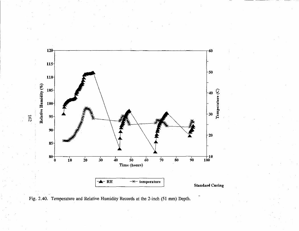
12.

115

11 ,...__ ~ ....,

105 ~ .• ... ·a

1 = = .. .. -= ...... .. 95 0\ -N .. i:r:

9

85

8 0 10 20 30 40 so 60 70 80 90

Time {hours)

,...._RH ~ temperature


50

40 Q: t ! E .. ...

30 ~ .E-<

20

10 100

Standard Curing

105 50

,...... 10 lffe

'-' ,...... ~ 40 u

'-' ·~ ::: .... ·~ e =

95 ~ = :: = " !:! "'

30 e <= " .. ~

.... - -0\ i:1i! 9 I w

20 85

8 10 0 10 20 30 40 50 60 70 80 90 100

Time (hours)

1-RH -- temperature Standard Curing


35

3 ,..... <;,) ....., t .. - 25 I? .. ... e - E!: °' .j>. 2

15

0 10 20 30 40 50 60 70 80 90 100 Time (hours)

1- 1" (25 mm) ---*"- 2" (51 mm) -H- 4" (102 mm) Standard Curing

Fig. 2.42. Temperatures at Different Depths.

CHAPTER 3: ANALYSIS OF CONCAVE CURLING IN PAVEMENT 1

ABSTRACT

A concrete pavement curls to a concave configuration when it is subjected to a

negative temperature gradient, which results when the temperature at its bottom surface is

higher than at its top surface. A gap may occur between the bottom of the slab and the

subgrade if the temperature gradient is large. This chapter offers an analytical approach to

the determination of displacement and stress distributions for a semi-infinite slab and for an

infinitely long slab of a finite width, which takes'into account a gap which may occur under

the slab resulting from curling. The elementary plate theory is applied to the slab resting on

a Winkler foundation.

The analysis for thermal stresses in a curled pavement slab developed by Westergaard

assumes a spring model to represent the subgrade support as a Winkler foundation. The

approach adopted by Westergaard is not valid for the case where a gap exists, although it has

been widely employed without respect to the effect of the gap on the resulting stress

distribution. This chapter examines a critical temperature difference between the bottom and

the top slab surfaces at the threshold of gap formation at the slab/subgrade interface in terms

of the concrete elastic constants and density, the thermal expansion coefficient of the

concrete, thickness of the pavement, and the modulus of the foundation support. If the

temperature difference is below the critical value, it is shown that Westergaard's solutions

are valid. Based on the solutions presented herein, correction of the coefficients in

Bradbury's approximate formula for the maximum stress in a finite pavement are suggested.

3.1. INTRODUCTION

A concrete slab will tend to curl when it is subjected to a temperature gradient

extending vertically through the slab thickness. The tendency to curl induces stresses in the

1 Contents of this chapter are published in "Analysis of Concave Curling in Concrete Slabs" By Tianxi Tang, Dan G. Zollinger and Sanjaya Senadheera in Journal of Transportation Engineering, Vol.119, N0.4, Jul.I Aug. 1993, pp. 618-633.

179

pavement as the pavement is restrained by its weight and the support pressures from the

subgrade (or foundation). The thermally induced stress caused by such interaction can be a

significant factor in contributing to early pavement cracking. This set of circumstances may

be critical, particularly within a few hours after placement since concrete is in the early stage

of hydration such that the strength may be insufficient to prevent cracking. Research has

shown (Emborg, 1991) that temperature rise caused by hydration does not immediately

produce thermal stresses because of the process of stress relaxation or creep in the concrete.

Thermal stresses arise when the temperature drops after its peak value and the concrete has

taken on a set. However, the temperature gradient which causes the slab to curl, as affected

by the heat of hydration, could be greater than that caused only by the effect of ambient

temperature and solar radiation. Therefore, analysis of thermal strains, as generated from all

sources of heat, is especially important for a curled slab at a very early concrete age.

Westergaard's solution (Westergaard, 1926) has been widely used in estimating

thermal stresses in curled concrete pavements (e.g., Yoder and Witczak, 1975; and Okamoto

et al., 1991). In his solutions, temperature change is assumed to be linear through the

thickness of the pavement, the concrete is assumed linear elastic, and a spring model is used

to define an elastic subgrade or a Winkler foundation. However, when the temperature

difference between the bottom surface and the top surface of the pavement slab exceeds a

critical value, the pavement may be so curled that a length of it near the slab edge separates

from the subgrade and a gap between the slab bottom and the subgrade results. Although no

mutual action exists between the separated portion of the slab and the subgrade, the spring

model in Westergaard's solutions is assembled over the entire slab bottom. A modification

to the Westergaard analysis is suggested which provides a separation of the spring model

from the portion of the slab which is free from the subgrade so as to more appropriately

reflect actual slab behavior. The Westergaard analysis provides expressions for displacement

and stress distributions for a semi-infinite slab and an infinitely-long slab of a finite width.

For a slab of finite dimensions, Bradbury (1938) suggested an approximate formula to

estimate the maximum stress, where two coefficients were given based on the Westergaard

analysis. Consequently, modifications of the Westergaard analysis can be encompassed

within modifications for curled slabs which all account for slab lift off at the slab edge.

180

3.2. BASIC EQUATIONS

Solutions of this study are, in a general sense, solutions to thermal stress and

displacement distributions in an elastic plate resting on a Winkler foundation, and

consequently, are applicable to concrete pavements.

The subgrade reaction of a Winkler foundation is expressed as (Scott, 1981):

q = -kw. (3.1)

where q is the subgrade stress on a unit area, w is the displacement of the slab, and constant

k is called the Foundation Modulus. The minus sign in Equation (1.1) indicates that the

reaction occurs in the opposite direction of displacement w. When the temperature in a

pavement slab is uniformly distributed, the slab theoretically remains planar, that is,

accompanied with a uniform vertical subgrade displacement. By denoting p and h as the

density and thickness of the concrete slab, respectively, one obtains the vertical displacement

due to the weight of the slab as:

w = ph 0 k

(3.2)

If the pavement slab is subjected to a negative temperature gradient through its thickness

(where the temperature of the slab bottom is higher than the temperature of the slab surface),

the slab tends to deform with its edges in an upward position, which contributes an additional

component of deflection. Thus, the total displacement of the slab in the downward direction

can be decomposed into two parts: w0 and w, that is, w,0 ta1=w0 +w, where w can be

determined by the following equations of the elementary plate theory and appropriate

boundary conditions for a weightless slab with a uniform temperature gradient (Westergaard,

1926):

= .E_ (M _ vM) + oult Eh 3 x Y h

(3.3)

181

and

- E_ (M - vM) Eh3 Y x

at.t + --

h

12 (1 + v) M . E h 3 xy

(3.4)

(3.5)

The displacement w is in the z direction (Fig. 3.1), and E, v and a are respectively Young's

modulus, Poisson's ratio and the thermal expansion coefficient of the slab. The moments in

Eqs. (3.3) to (3.5) and shear forces are denoted as positive when their directions are the

same as shown in Fig. 3.2. The temperature difference t.t is assumed to vary linearly

between the slab bottom surface and the slab top surface with no temperature change at the

mid-plane of the slab. When the temperature at the top surface is lower than at the bottom

surface, t.t is denoted as positive.

3.3. STRESSES IN AN INFINITE PAVEMENT

When the pavement slab is considered to be of infinite extent with respect to the

width and length of the slab, the tendency to curl is fully restrained or w = 0 such as

M,=MY= Eh 2at.t

12 (1 - v)' M = 0 xy

(3.6)

With a positive t.t, the maximum tensile stress is at the top surface of the slab either in x or

y direction, whose value is:

(f = 0

Eat.t 2 (1 - v)

(3.7)

If E = 3 X 106 psi (2070 MPa) , v = 0.15, a = 6 X l0-6/°F, k = 100 lb/in3 (27.1

MN/m3), and t.t = 22.2°C (40°F), then u

0 = 424 psi (2.92 MPa) according to Eq. (3.7).

These parameters will be employed in other examples in this chapter without further

182

x -~

/

/ •/ ,,.

/·: ----------------------------------- -----/" ,.. _________________________ _

-00 (.;.)

/' ,'' /' / ,'

/. ,. ,'

0 /. , , -·-·-·-·-·-·-·-·-·-·-·-·-·- -·-·-·-·-· ,,r·~-·-·-·-·-·-·-·-·- -·-· /" j,'

/. , i /. , ,,' i /'

/. ,' /. ,'

/' ,' /. ,'

/ ,' /' , ,

/. ,'' Top Surface

/ ,' // L..'.'---~~-+---=B:--o-:t:-:-t-o-m-=s:--u-r-=f-a_c_e_,

/

Fig. 3,1. A Pavement Slab with the Coordinate System.

y ·-·-·-·-·--~

/ /

/ /

/

.1'x /

/ /

/ My

0 !':--·-·-·-·-·~ y

dz

' z

q

Mx+dMx

~ Mxy+dMxy

I jax+dQx

Mxy Q x l .. ' ...... I · ..

"""'" I

My+dMy

r---------.' ,

Mxy+dMxy

Q y +dQ y

Fig. 3.2. Stress Resultants Acting on Plate Element.

comment unless otherwise indicated. Infinite slab behavior can be considered to apply to the

area that is far enough from the slab edges.

3.4. STRESSES IN A SEMI-INFINITE PAVEMENT

A pavement slab with an edge at y = 0 that is assumed to be infinite in the positive y

direction and in the positive and negative x directions is shown in Fig. 3 .1. The slab

behavior in this instance is independent of x. Combining Eqs. (3.3) and (3.4), one obtains

(Westergaard, 1926):

MY = Eh 3

[- d

2w. _ (1

dy2 + v) cxdt]

h . 12(1 - v2}

Static equilibrium requires:

= kw

for a slab element that is in contact with the subgrade. For the portion of the pavement

which is in contact with the subgrade, the following equation, from Eqs. (3.8) and (3.9),

holds:

(3.8)

(3.9)

Eh 3 d 4w dy•

+kw = 0 (3.10)

or c• a•w dy•

+ w = 0, f = 4

Eh 3 (3.11)

12 (1 - v2}k

where f is called the radius of relative stiffness. The general solution to Eq. (3.11) which

satisfies, the condition w = 0 at y = oo is:

185

w = __ Y_

e J T t. (3.12)

With the boundary conditions moment My = 0, shear force QY = 0 at the edge y = 0, one

obtains:

= _ £2 (1 + v) Ol!:;.t =

h

which the associated displacement is (Westergaard 1926):

w = -w '2cos [-y- + ?r] e-J~t $0 VL r;:;- 4 '

y2£

(3.13)

= £2 (1 + v)Ol!:;.t w,o h (3.14)

where w,0 is the magnitude of the displacement at the edge y = 0. The stress in y direction

at the top surface is (Westergaard 1926):

__ Y_

e J z- t '

(3.15)

which is the maximum tensile stress within the cross-section of the slab parallel to the x axis.

The stress in x direction at the top surface can be calculated by using the following

relationship (Westergarrd 1926):

(3.16)

These solutions are valid for a slab which remains in contact with the subgrade whether the

slab is subjected to a negative or positive temperature gradient. Nevertheless, when !:;.t > 0

(the temperature at the top surface is lower than at the bottom surface) the pavement is

186

curled such that the displacement at the edge w (y=O) = -W50• Therefore, the necessary and

sufficient condition for Eq. (3.9) to be valid is:

or [ ;f ] 2

-k(-1 2-:-V)-OI

(3.18)

where (.:it)sc is the critical temperature difference for the semi-finite pavement, since it is the

maximum temperature difference correlating to impending slab lift off.

When the temperature difference is larger than (.:it)5., the length of slab lift off, s, is

assumed to separate from the subgrade surface (Fig. 3.3). When the x=O is positioned at the

end of the length s rather than the edge of the slab as shown in Fig. 3.3, the governing

equations for the part -s :5 y :5 0 are provided by Eq. (3.8) and the following equation:

= -ph.

Combination of Eqs. (3.8) and (3.19) yields

Eh 3 d4w ---- -- - ph = 0 . 12 (1 - v2

) dy 4

(3.19)

(3.20)

The boundary condition for this portion is My = 0 and QY = 0 at y = -s. The general

solution for the displacement w, Eq. (3.12), is still applicable for the slab portion between

the limits 0 :5 y :5 + oo, but the coefficients A1 and A2 and another unknown s should be

determined to comply with the boundary condition at y = 0: w = -w0 , and w and its

derivatives with respect to y are continuous. In terms of loads, the boundary condition at y

= 0 can be summarized as (Fig. 3.4):

187

//" _____ _

...... 00 00

~-------------- --- -

Wtotal Wo

·-: ... ·-:=: :=:=:=: :=: ·=:=:=.=:=:=:=:=:=:=:=:=:-·-·-: ........... :=:-·-·-·-·-·-·-·-·-·-·-·-·-·-·-·-·-·-·-·-·-·-·-·-·-·-·-·-·-· .... I i i i I i i I i i i i I

i Zf

y

w

Fig. 3.3 Sketch of an Up-Curled Semi-Infinite Pavement Slab

Mo y

0 ·-·-·-·-·-·-·-·-·-·-·-·-·-·-·-·-·-·-·-·-·-·-·-·-·-·-·-·-·-·-·-·-·-·-·-·-·-·-·-·-·-·-·-·-·-·-·-·-·-·-·-·-·-·-· ......

Fig. 3.4 Mathematical Model for the Up-Curled Semi-Infinite Slab

MY = -M. = - .!. phs2 2

Qy = -P = -phs at y = 0. (3.21) 0

w = -w.

The results are:

(3.22)

(3.23)

and s

= ,,-1, (3.24)

where (3.25)

Therefore,

w __ Y_

w = --0- COS [ _L +\OJ

e J TI (3.26) COS\O /2£

,

and

ITY = er. [ 1 -w.

sin [;,,··]-~]. (3.27) W,

0COS\O

190

where

cos 'P 1

(3.28) J2(2°/-2y+ 1)

Note that solutions (3 .26) and (3 .27) are for temperature differences dt ~ (/J,.t),c In the

extreme case, where /J,.t = (/J,.t) 8c or w,0 = w0 , and hences = 0, and <p = 11"14, Eqs. (3.26)

and (3.27) become identical with Eqs. (3.14) and (3.15). Differentiating the right side of

Eq. (3.27) and equating it to zero, one concludes that uY reaches its maximum value at

y - fl £( 511" 14 - <p).

With the parameters used in the previous example and p = 0.087 lb/in3 (2.4 g/cm3)

and h = 8 in (2.03 cm), the following is calculated:

£ = 33.8 in (85.9 cm),

/J,.t = 40°F (22.2°C) > (dt),c = 14.13°F (7.85°C) or

w,0 = 0.0394 inch (1.001 mm) > w0 = 0.00696 inch (0.177 mm).

Eqs. (3.14) and (3.15) are not valid in this instance. From Eqs. (3.24), (3.26), and (3.27),

one obtains:

s = 1.37£ = 5.46 ft (166 cm), and

<p = 75.1°.

Displacement and stress distributions with these parameters calculated with Eqs. (3.26) and

(3.27) are shown in Figs. 3.5 and 3.6, where abscissa 0 represents the edge of the slab and

s/112£ represents the location of the x axis shown in Figs. 3.3 and 3.4. As seen in the

figures, Westergaard's solutions without consideration of the gap effects overestimate uy for

the range 0 < (yN2£) < 3. 7 . As illustrated, stress Uy approaches u0 when (y/1/2£) is

approximately 6. For y > 6\/2£, the slab behavior can be considered to be infinite.

191

w(mm)

3

2.5

2

1.5

.----------------------------.-0.12

s --12 e

w(in.) 0.1

0.08

0.06

0.04

0.02

0

-0.5+-----~----------r-----------,------t--0.02 0 1 2 3 4 5 6

j ....... Westergaard -- This Study

(y + s)

12 e

Fig. 3.5. Stress Distribution for an Up-Curled Semi-Infinite Slab.

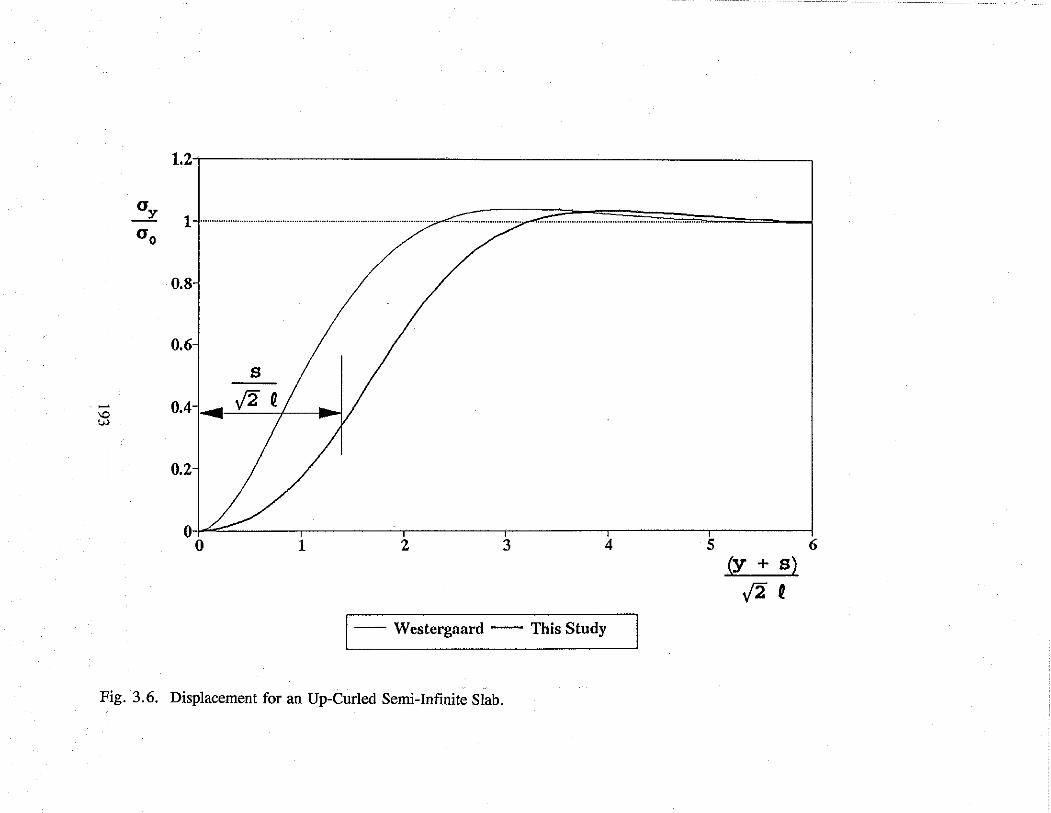
1.2.--r·---------------------------,

1 ........................................................................................... .............................. . ........................................................ .

0.8

0.6

0.2

01+0~:::::_--,1-----'-•2----,3----,4----sr----~6

1-- Westergaard -- This Study

Fig. 3.6. Displacement for an Up-Curled Semi-Infinite Slab.

(Y + s)

..f2 e

3.5. STRESSES IN AN INFINITELY LONG PAVEMENT OF A FINITE WIDTH

For the condition where the pavement slab is infinite in both the positive and negative

x directions with a finite width of bin they direction (-b/2 s; y s; b/2), the problem is

symmetric with respect to the x axis. The general solution to Eq. (3 .10) becomes:

- B y h y B . y "nh y w - I COS-- cos -- + 2 sm-- SI --

ff£ ff£ ff£ ff£ (3.29)

Then the corresponding uY is:

(3.30)

For a slab in full contact with the subgrade, Eqs. (3.29) and (3.30) must satisfy the boundary

condition:

MY = 0 } Qy = 0

b at y = 2

such that

and then

2(tanm - tanhm) cosm coshm B1 = w,o --'--~~---'-~~---

sin 2m + sinh 2m

2(tanm + tanhm) cosm coshm sin2m + sinh2m

194

(3.31)

(3.32)

(3.33)

w = -w 2cosm coshm [(-tamn + tanhm)cosLcoshL bo - sin2m +sinh2m fi f fi f

+ (tamn + tanhm)sin_Y_sinh_Y_] . {if {if

(3.34)

and

" = " [ 1 _ 2(tanm -tanhm) cosm coshm sinL sinhL Y

0 sin2m +sinh2m fi f fi f 2 (tanm + tanhm) cosm coshm ~sL coshL] ,

sin2m + sinh2m fi f fi f

(3.35)

where m = b/(zVU), -wb0 is the displacement at y = ±b/2, and

w = w - sin2m + sinh2m bo '

0 sin2m + sinh2m (3.36)

Solutions (3.34) and (3.35) were given by Westergaard. Similar to the semi-infinite case,

when At > 0, uY is the maximum tensile stress in they direction within the cross-section

parallel to the x axis, located at the top surface. The stress in the x direction at the top

surface is determined by Eq. (3 .16).

Displacement and stress distributions shown in Eqs. (3.34) to (3.35) are valid only

when:

(3.37)

or h 2p sin2m + sinh2m

[ ]

2

{if k (1 + v)a [ -sin2m + sinh2m)' (3.38)

where (At)bc = (At)sc (w,jwh0 ) is the critical temperature at which slab lift-off occurs for the

infinitely long pavement of a finite width.

195

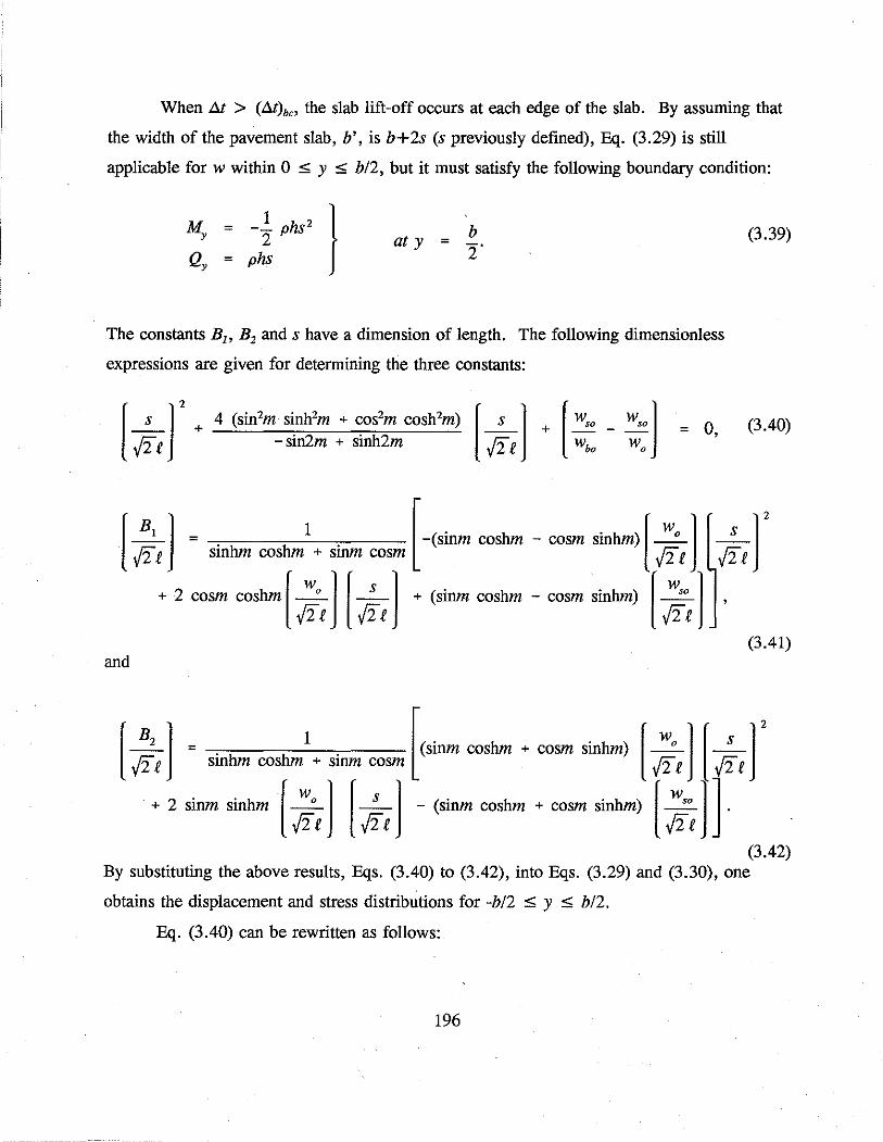
When t.t > (t.t)b<> the slab lift-off occurs at each edge of the slab. By assuming that

the width of the pavement slab, b', is b+2s (s previously defined), Eq. (3.29) is still

applicable for w within 0 ~ y ~ b/2, but it must satisfy the following boundary condition:

MY = -; phs2 )

Qy = phs

b at y = 2·

The constants B1 , B2 and s have a dimension of length. The following dimensionless

expressions are given for determining the three constants:

[ s ] 2

+ 4 (sin2m s~nh2m + ~os2m cosh

2m) [-s-] + [ w,0 _ w,o]

.j2 f - sm2m + smh2m .j2 f who w 0

= 0,

[ BJ 1 [ [w] _1_ = -(sinm coshm - cosm sinhm) - 0

-/2 f sinhm coshm + sinm cosm .j2 f

+ 2 cosm coshm ( w0 ] [-s-] + (sinm coshm - cosm sinhm) ( w,0

)

/2f /2f /2f

and

(3.39)

(3.40)

(3.41)

[!2_] = . 1

[(sinm coshm + cosm sinhm) r~J [-s ] 2

.j2 £ smhm coshm + sinm cosm .j2 £ .j2 £

+ 2 sinm sinhm ( ;f) ( ;f) -(sinm coshm + cosm sinhm) ( ~ J]. (3.42)

By substituting the above results, Eqs. (3.40) to (3.42), into Eqs. (3.29) and (3.30), one

obtains the displacement and stress distributions for -b/2 ~ y ~ b/2.

Eq. (3.40) can be rewritten as follows:

196

(3.43)

where 'I/ = (-sin2m + sinh2m)/2(sin2m sinh2m + cos2m cosh2m) and m = b/('2>12£) = (b'-

2s)/('2>12£). Eq. (3.43) for b ors is nonlinear for a specified b' since 'I/ and (w,,)w,0 ) are not

constant, but can be determined by iteratively solving the results using the quadratic formula.

The relations for the dimensionless quantities 'I/ and (wbjw,0 ) versus the normalized length m,

respectively, are shown in Fig. 3.7. These two curves provide an initial estimate of b ors

value in the iterative process. When the slab is wide enough, both 'I/ and (wbjw,0 ) approach

unity, and then Eq. (3 .43) can be simplified as:

or s =rw:--1 .;u- J w:-

(3.44)

(3.45)

which is identical to Eq. (3.24) for a semi-infinite slab. Eq. (3.45) may be taken as an

approximation for determining s when m is not too small. Judging the expressions for 'I/, wbo

and w,0 , one finds that both 'I/ and (wbjw,.,) approach unity as sinh2m > > 1 or m > > 1. If

ans value obtained from Eq. (3.45) results in m > > 1 for a specified b', behavior of slab

of corresponding width can be approximately considered to be a semi-infinite slab.

If the width of the slab is assumed as b' = 24 ft (7.3 m) as in a highway pavement

before the longitudinal joint is formed, the lengths b ands can be determined with Eq.

(3.43). First, ans value is solved from Eq. (3.44) as the initial value of s for iteration,

which is s = 5.52 ft (168 cm) or stv'2£ = 1.38. By substituting this s value in 'I/ in Eq.

(3.43), the second value of s is obtained. After four runs of iteration, an accurate s

197

~o -- and T) W.o

1

·············· ... ···· ········· ,..._,......,, ... ~·~:::::::::::::::::::::":":"7"'=--.,~~~~~~J .· ····· .· ..... . : ······························· . .·

?"] /

0.8

0.6

0.4

0.2

:

0 1 2 3 4

m Fig. 3. 7. Stress Distribution for an Up-Curled Infinitely Long Slab of a Finite Width.

value appears, which is s = 5.72 ft (174 cm) or sfl/2£=1.43. The displacement and stress

distributions calculated from this value are shown in Figs. 3.8 and 3.9. Since the strength of

concrete at early ages can be rather lower than that when concrete is mature, analysis of

thermal stresses in concrete pavement slab before the longitudinal joint is formed is

significant.

Location and the magnitude of the maximum <Ty in an infinitely long pavement of a

finite width can be acquired by maximizing <Ty in Eq. (3.30). When mis not too small, the

slab behavior along the slab edge may be assumed to be semi-infinite. Accordingly, the

maximum <Ty may be obtained by simply substituting y = V2f(5?r/4 - \0) to Eq. (3.27).

3.6. MAXIMUM STRESS IN A FINITE PAVEMENT

When a slab with a finite length Lx and a finite width Ly on a Winkler foundation is

curled in a concave configuration as subjected to a negative temperature gradient,

displacement and stress distributions can also be found analytically, where the governing

equations are not ordinary differential equations but partial differential equations. For

estimating the maximum <Ty in a finite slab, Bradbury (1938) proposed an approximate

formula as follows:

(f = EOLlit

2 (3.46)

where the coefficients C1 and C2 for the appropriate slab dimensions were given based on

Westergaard's stress solution Eq. (3.35) for an infinitely long slab of a finite width in terms

of the ratio of the maximum <Ty I <T 0

• In the cases where the temperature difference exceeds

the critical temperature difference (Jit)bc• the Bradbury coefficients should be corrected. By

combining Eq. (3.35) and Eqs. (3.40) to (3.42), the ratio of the maximum <Ty to <T"' C1 or C2,

is obtained for values of m. Fig. 3.10 shows an example of application for lit = 40°F

(22.2 °C), where the relation of C (C1 or C2) in terms of the ratio of d ( = Lx or Ly) to f,

rather than m, is given. It should be noted that the curve determined by this study is

dependent on the temperature difference, because the length s is dependent on the

199

IV 0 0

w(mm)

1.5 s -

1

0.5

,/ ,,/'

, , .

; ,·''

./ /

/ ,

w(in.)

0.06

0.04

0.02

/' ,., 0 ........................................................................................................................................................ ;,,.,............................................................................................. 0 _ .. __ .... --.... ____ ,. ________ ,, ______ ··--- -~

---·--·--------- ........... -.. ..

-0,5:-1-----~---.---~----.-----.----_,.-----r--o.02 o ~5 1 1.5 2 ~5 3 15

\ ·····-- Westergaard - This Study

Fig. 3.8. Displacement Distribution for an Up-Curled Infinitely Long Pavement of a Finite Width.

1 ................................................................................................................................................................................................................... ..

0.8

s 0.6 12 e

N 0 ~

0.4

0.2

0.5 1 1.5 2

1-- Westergaard -- This Study

Fig. 3.9. Coefficients in Equation (3.43).

2.5 3 3.5

temperature difference for a specified slab. However, there appears to be no significant

differences between the curves shown in Fig. 3.10. This analysis provides improved values

for coefficients C1 and C2 , and confirms that Westergaard's solution is applicable in

estimating the maximum stress (not the stress distribution) in the slab without significant

errors in a wide range of temperature differences. When the temperature difference between

the bottom surface and top surface of the slab is large enough, modification of C1 and C2

based on the solutions of this study is appropriate.

The above analysis is applicable to slabs with free boundary conditions. For the case

where the slab edge is restrained, displacement and stress solutions are provided in the

following section.

3.7. STRESSES IN A CURLED SLAB WITH ITS EDGE RESTRAINED

When a slab with its edge restrained is curled as subjected to a negative temperature

difference, displacement and stress distributions still can be found. Generally, the restrained

edge may be assumed to be connected to the subgrade or a neighboring structure through two

springs: Kh for the translational stiffness and K, for the rotational stiffness. For example, a

U-shaped drain structure connecting two concrete slabs may be simplified as a rotational

spring.

As an example, a semi-infinite slab on a Winkler foundation with its edge restrained

by a rotational spring K, is analyzed. When the temperature difference !:.t is not very large,

all the slab is in contact with the foundation. Eqs. (3.8) to (3.12) are valid in the case, but

the boundary condition (Fig. 3.4) is My = -M0 = K,00 and QY = 0 at y = 0, where 00 is the

rotation of the end surface y = 0. Thus, the displacement and stress solutions are obtained

as follows:

[ M J [ ) __ ,y w = - w --0

. .ficos _Y_+?r e ~Tl, ,0 k£2 fit 4

(3.47)

202

IV 0

"'

c

1.Z . ....-----.!-----,i----,.!---D-. ,.$_[jJ_lfJ_lfJ---;9-.IEJ-tEJ-. -lEl--rl-ij;;l_.q;J_.q;J--,n

. o+

"' ------+- - ------rnc- ---1 ---- - ----i- -- ----J-- -- ----+-- ------

0.2- ........ . .......... \ .. ··~-0 ........ \···

i+'b Offi~B+sei'Wll""'~i--.~~~i--~~~i--~~---;,~~~---;,~~~---;,~~~--J

0 2 4 6 8 10 12 14

D Westergaard + This Study

Lx or LY

e

Fig. 3.10. Coefficients for the Maximum Stress in a Finite Pavement Slab Curled Up Due to Temperature Gradient.

<J = <J [1 -(1 _ 6M0 ]{isin[L+11"]e-J~t], y o <Joh2 {if 4

and M = () K = o o r

wsoKr f K, _+_ fl kf'

These solutions are valid under the following condition:

or

M W __ o =:;:; Wo

so kf2

!::i.t :;;(t.t) [ l+ {iK,] = (t:i.t)sc(l+t) SC kf3

(3.48)

(3.49)

(3.50)

(3.51)

where .I = fY2K,)l(kf3). As seen in Eq. (3.51), the critical temperature difference is raised

because of the existence of the spring support at the slab edge. When the temperature

difference t:i.t is so large that Eq. (3.51) is not satisfied, there would be a portion of the slab

separated from the subgrade.

Similar to the case shown in Fig. 3.3, the part of the slab (-s :;::; y :;::; 0) is free from

the subgrade and governed by Eq. (3 .20), but its edge y = -s is restrained by a rotational

spring K" while the rest of the slab (y ~ 0) is governed by Eqs. (3.8) and (3.9). In this

case the boundary condition is MY = -M0 = -K/Js and QY = 0 at y = -s, where Os is the

rotation of the end surface y = -s, and w = w0 at y = 0. Certainly w, () (= dwldy) and the

third and fourth derivatives of w with respect to y are all continuous at y = 0. The

displacement and stress distributions are dependent on the length s:

204

w [;£ +~] __ Y_

w = --0- COS e J z- t

cos~

(3.52)

and [ 1 -

WO sin [ ;,, . ·] ,-*'] . <Iy = <Io

w,0cos~

(3.53)

where

cos~ = 1

1+ (1+~12 ./2£

(3.54)

The length s is determined by the following equation:

~r[-s J3

+(1+2r)[_s J2

+(2+2r-,,2r)[-s J+(l+f-,,2) = o.

3 ./2£ ./2£ ./2£ (3.55)

where I' = V(w,jw0 ) and f = r/2K,)/(k£3) as noted before. Eq. (3.55) is reduced to Eq.

(3.24) when there is no restraint at the slab edge, that is, K, = 0 .

3.8. CONCLUSIONS

Displacement and stress distributions are provided for a semi-infinite and an infinitely

long slab of a finite width on a Winkler foundation as the slab is subjected to a negative

temperature gradient that takes into account that a gap can form between the slab edge and

the subgrade. A critical temperature difference for each of the cases is noted such that when

the temperature difference is greater than the critical value, the gap occurs and solutions of

this study apply.

When an infinitely long strip of pavement is wide enough, it can be considered as a

semi-infinite pavement for determining stress and displacement distributions. This chapter

gives a procedure to judge if the width of the slab is "wide enough."

205

For a finite slab curled in a concave configuration due to the negative temperature

gradient, the maximum stress in either direction with sufficient accuracy may be

approximately estimated with Bradbury's formula. The coefficients in the formula can be

determined with the stress solution for the infinitely long strip of pavement.

3.9. APPENDIX I: REFERENCES

Bradbury, R. D., Reinforced Concrete Pavement, Wire Reinforcement Institute,

Washington, D.C., 1838, pp. 34-41.

Emborg, M., "Thermal Stress in Concrete at Early Ages," Analysis of Concrete

Structures by Fracture Mechanics. L. Elfgren and S. P. Shah, eds., Chapman and Hall,

New York, 1991, pp. 69-87.

Okamoto, P.A., Nussbaum, P. J., Smith, K. D., Darter, M. I., Wilson, T. P., Wu,

C. L., and Tayabji, S. D., Guidelines for Timing Contraction Joint Sawing and Earlier

Loading for Concrete Pavements, Report No. FHWA-RD-91-070, Federal Highway

Administration, McLean, Virginia, 1991.

Scott, R. F., Foundation Analysis. Prentice-Hall, Eaglewood Cliffs, New Jersey,

1981, pp. 119-201.

Yoder, E. J. and Witczak, M. W., Principles of Pavement Design. 2nd Edition, John

Wiley & Sons, New York, 1975, pp. 85-86.

Westergaard, H. M., "Analysis of Stress in Concrete Pavements due to Variations of

Temperature," Proceedings of Sixth Annual Meeting, Highway Research Board, 1926, pp.

201-205.

206

3.10. APPENDIX II: NOTATION

The following symbols are used in this pages:

E

h

k

=

=

Young's modulus;

pavement depth;

foundation modulus;

Kh = translational stiffness;

K, = rotational stiffness;

f = radius of the relative stiffness;

M = moment on the cross-section of the pavement;

q = reaction by the foundation;

Q = shear force on the cross-section of the pavement;

w = displacement in the z direction;

a = · thermal expansion coefficient;

At = temperature difference between the bottom surface and the top surface

p =

(J =

(Jx =

<ly =

of the pavement;

Poisson's ratio;

maximum tensile stress in the y direction;

stress in the x direction at the top surface of the pavement; and

stress in the y direction at the top surface of pavement.

207

CHAPTER 4: FRACTURE TOUGHNESS OF CONCRETE AT EARLY AGES'

ABSTRACT

This chapter reports the experimental results involving the application of the size

effect law to early-age concrete for determining the material fracture parameters K1r and

Cr. These parameters were determined for concrete with several different coarse

aggregates at 1-day age, showing that this test method is applicable both in the laboratory

and at the construction work site. Tests for concrete at different ages from 112 day to 28

days showed that early-age concrete is more brittle than mature concrete. Increases in Krr

and Cr with concrete age are observed. The Krr and Cr values at early ages may be used

as a criterion to evaluate concrete quality.

4.1. INTRODUCTION

Since linear elastic fracture mechanics (LEFM) was applied to concrete by Kaplan

in 19611, several investigations have measured apparent values of the critical stress

intensity factor K1c for cement paste, mortar and concrete specimens at their early ages.

For example, Naus and Lott2 showed, by testing notched 4 x 4 x 12 inch (10.2 X 10.2

X 30.5 cm) and 4 x 4 x 14 inch (10.2 X 10.2 X 35.6 cm) concrete beam specimens,

that the apparent value of the critical stress intensity factor K1c increased as the curing

time was increased from 3 to 28 days. Test results indicated that the corresponding

increase for concrete using a river gravel coarse aggregate was 54.2% and for concrete

using a crushed limestone as its coarse aggregate, K1c increased 23.0%. It was also

noted in this study that as the length of moist cure was increased from 28 days to 90

days, the increase in K1c was 7% for the concrete containing river gravel while there was

no apparent change in K1c for the concrete with the crushed limestone. Ojdrovic, et al. 3

1 Contents of this chapter are published in "Fracture Toughness of Concrete at Early Ages" by Dan G. Zollinger, Tianxi Tang and Rae H. Yoo in the ACI Material Journal, V.90, No.5, September-October 1993, pp. 463-471.

209

tested notched split-tension cylinders of concrete with the maximum aggregate size of 9.5

mm, in which the coarse aggregate type and the specimen size were not reported. Their

tests showed that K1c increased with the concrete age from 1-day to 28-day age. The

value of K1c at 1-day age was approximately 45% of the K1c at 28-day age. Although

these observations indicated the trend of rapid increase in the apparent value of K1c with

concrete age within 28 days, they also provided a great deal of evidence for dependence

of K1c on the concrete specimen geometry and size. In other words, the critical stress

intensity factor K1c based on LEFM and brittle fracture concepts does not constitute a

material constant for concrete.

With the development of the nonlinear fracture mechanics of concrete, which takes

into account the effect of the process zone at the crack tip, RILEM has tentatively

recommended two effective (or equivalent elastic) crack models, Jenq and Shah's two

parameter fracture model4 (TPFM) and Bal:ant's size effect laW' (SEL), for determining

the fracture parameters of concrete which are· material constants, and independent of

specimen geometry and size. These models characterize the fracture process zone by an

effective crack length that can be determined from an additional instability condition.

Recently, Wong and Miller6 measured the two material fracture parameters defined in

TPFM, the critical stress intensity factor K1~ and the critical crack tip opening

displacement CTODc, for concrete at 1-day, 3-day and 5-day ages, and concluded that

K1~ increased with concrete age and that early age concrete was more brittle than mature

concrete. Our work tends to confirm the findings of the earlier studies by Shah, et al.7

This chapter presents the results of an experimental investigation on concrete at early

ages based on SEL. Fourteen batches of concrete beams using different coarse

aggregates with the maximum size of 19 mm or 38 mm were produced and tested one

day after casting in laboratories or at work sites to obtain Km the critical stress intensity

factor (or fracture toughness) in the infinite specimen, and cf, the effective critical crack

length (or the process zone size) in the infinite specimen, as defined in SEL. The value

of cf can be used to evaluate the brittleness of concrete structures as SEL suggests. Also,

concrete beams were tested at the ages of 1/2 day, 1 day, 7 days, 21 days and 28 days to

show increases in Krr and cf with concrete age.

210

4.2. RESEARCH SIGNIFICANCE

Failure of concrete is a process of crack formation and growth. With fracture

parameters defined in SEL, resistance of concrete material against fracturing can be

appropriately and correctly evaluated. Through this study, it is shown that the size effect

law originally proposed for mature concrete can also be applied to early-age concrete.

Since many cracks in concrete structures are initiated due to temperature and shrinkage

stresses at early ages, the understanding and determination of fracture toughness and

effective critical crack length of early-age coricrete are crucial for crack control.

4.3. SIZE EFFECT LAW

According to LEFM and brittle fracture concepts, material fractures failure occurs

when K1 reaches a critical value Kie· However, it has been long observed that a steady

crack growth takes place in concrete before the peak load. In addition, many

microscopic-scale investigations have indicated that a process zone exists around the

concrete crack tip8• Microcracking in the process zone consumes energy, and therefore,

toughens the material and causes nonlinear fracture behavior, which, in tum, results in

the size effect on the nominal strength of the concrete structure. The size effect law

proposed in 1984 by Bai.ant' gives a formula to describe the size effect for the

geometrically similar structures (or specimens) as follows:

Maximum uN = Bf.

(4.1)

where fu is the tensile strength of the concrete, d is a specimen dimension, B and d0

depend on material, structure geometry and load type. A modification of the size effect

law proposed in 1990 by Bai.ant and Kazemi9 attributes the nonlinearity of concrete

fracture in an infinite specimen to two material constants: the critical stress intensity

factor in an infinite specimen Km and the critical effective crack length or the process

211

zone size in an infinite specimen cf, from which B and d0 for any geometry and load type

can be derived through LEFM. (For expressions of B and d0 in terms of Km and cf, and

geometry, and load type and related LEFM formulas, see Appendix I.) Inversely, Kif

and cf can be obtained by a series of tests on the geometrically similar specimens of

different sizes. The three-point bending beam test has been suggested for this purpose10•

By using linear regression techniques, test data can be analyzed as follows:

Y* =A*X*+C*, (4.2)

where, for the three-point bending beam test, y• = (bd/P)2, x· = d, P = the peak load,

b = thickness and d = depth of the beam, and A• and c· are regression constants. (See

Appendix I for the general expression for any geometry and load type.) It has been

shown11 that, in the three-point bending test, the contact width of the load does not have a

significant influence on the stress distribution or the value of K1• Therefore, the load in

this test can be reasonably simplified to a concentrated point-load in analysis. An

advantage of the three-point bending beam test is that it is convenient to conduct and a

reasonable degree of accuracy is assured in the analysis of the test results. Based on the

regression constants A· and c·, Kif and cf can be calculated with:

and

K = j g(w) If A* '

c = J

c· K~ g' (wo)

=

(4.3)

(4.4)

where g'(w) denotes the derivative of a function g(w) with respect to w, and w is the ratio

of the crack length a to the specimen dimension d, g( w0 ) and g' ( w0 ) are values of

functions g(w) and g'(w) at w = ajd respectively, and a0 is the notch (initial crack)

length. It should be pointed out that function g(w) is dependent on the specimen

212

geometry. (For the definition of g( w) and its· form for the three-point bending beam

specimen used in this study, see Appendix I.

To characterize the brittleness of structural response, a number of so-called

brittleness numbers have been proposed12•

13•

9 and are summarized by Gettu et al14• The

brittleness number is defined as {3 = d/d0 by SEL and it can be calculated as

g(w;J d D = = (4.5)

where D = [g( w0)/ g' ( w0)]d is called the effective structural dimension. After the structure

dimension is thus accounted for, {3 is independent of the geometrical shape15•

4.4. EXPERIMENTAL PROGRAM

Materials and specimens

The coarse aggregates used in this study were obtained from stockpiles prepared

for concrete pavement construction projects. The coarse aggregate was of maximum size

of 3/4 inch (19 mm) or 1-1/2 inch (38 mm). Due to the effect of the coarse aggregate,

the sizes of the beam specimens in this study were larger, in general, than those which

have been reported in many references. Fig. 4.1 shows the geometry of the beam

specimen. The thickness of each specimen was 5 inches (12.7 cm). For concretes with

aggregate size of 3/4 inch (1.9 cm), depths of the specimens for each batch were 3 inches

(7.6 cm), 4.5 inches (11.4 cm), 6 inches (15.2 cm), 9 inches (22.9 cm) and 12 inches

(30.8 cm). For concrete with maximum aggregate size of 1-1/2 inches (3.8 cm), the

depth of 3 inches (7. 6 cm) is less than three times the maximum aggregate size so that

only the four largest specimen sizes were used. The ratio of the support span of the

beam (s) to the beam depth (d) was 2.5 for each specimen, and the ratio of the notch

length (~) to the beam depth was 0.25 for each specimen. The total length of the beam

specimen was 1.2 times as long as the support span. Therefore, all the beam specimens

were geometrically similar. The ratio of s/d for these specimens was 2.5 in comparison

to the ratio of s/d = 4 or 8 which is more frequently used in bending tests. This ratio

213

p

' .

·········~ 0 Jl

d

... x

s

Fig. 4.1. Geometry of the Three-Point Bend Beam Specimen.

was chosen since the support span was restricted by the dimension of the work table and

the allowable stroke of the testing machine. It is conceivable that the depth of 12 inches

(30.8 cm) may be close to the limit for most industry and research laboratories.

When the specimen is very thin, it can be simplified as a plane stress problem;

when the specimen is very thick, it can be simplified as a plane strain problem. Since

Poisson's ratio of concrete is small, the two extreme simplifications do not make

significant differences in stress distribution in the specimen, which allows the specimens

of different sizes to be of the same thickness. In this study, all the beam specimens were

5 in (12. 7 cm) thick, which is larger than three times the maximum aggregate size of 1-

1/2 inches (3.8 cm).

Fourteen different concrete batch designs were prepared and tested in this study.

Eleven of them were prepared in the laboratory and the remaining four were prepared on

site of concrete pavement construction projects.

Each of the ten batches prepared in the laboratory contained Type I cement and

Class C fly ash provided by the same manufacturer. Siliceous river gravel, crushed sand

stone, and crushed limestone from different sources in Texas were used as coarse

aggregates. Physical properties and gradations of these aggregates were examined by

following test standards: ASTM Designation C 127 and C 12816, Test Method Tex-403-

A, Test Method-405-A and Test Method-401-A17• The results are listed in Tables 4.1 to

4.3. Table 4.4 gives the mix proportions based on one-sack of cement (43 kg or 94 lb).

These mix designs were based on designs which were used in concrete pavements

constructed in Texas, using slip-formed paving techniques which range in slump from 1

to 2 inches (2.5 to 5.1 cm).

A series of concrete batches using a siliceous river gravel, designated as G2 in

Table 4.4, were prepared. Two batches of specimens were cast indoors at the room

temperature of approximately 73 F (22.8 C) and another batch of specimens was cast

outdoor under ambient conditions at temperatures near 95 F (35 C). One set of

specimens cured under indoor conditions contained an unwashed coarse aggregate while

another set that was cured indoors contained an coarse aggregate that was thoroughly

215

Table 4.1. Physical Properties of the Aggregates.

Aggregate I.D. SSD Specific Gravity

SRG Gl 2.467

SRG G2 2.646

SRG G3 2.588

SRG G4 2.796

css 2.499

CLLl 2.600

CLL2 2.566

CLL3 2.688

Dolomite 2.757

Sand 2.441

Note: SRG - Siliceous River Gravel, CSS - Crushed Sandstone, CL - Crushed Limestone, DM - Dolomite

Bulk Specific Gravity

2.411

2.604

2.580

2.783

2.405

2.566

2.517

2.676

2.730

2.331

Absorption Percent Solid Capacity(%) (%)

2.27 57.81

1.59 60.70

0.33 58.73

0.46 54.28

3.76 55.31

1.31 56.25

1.91 55.78

0.46 53.21

0.99 54.10

5.31 69.13

cleaned. All other specimens were cured indoors at the room temperature of 73 F

(22.8 C).

A series of specimens that were cast using mix design G 1 consisted of five batches

which were tested at 1/2-day, 1-day, 7-day, 21-day and 28-dayages (one batch per age).

Fracture tests were performed only at a concrete age of one day for all other specimens.

The concrete beam specimens were cast in steel molds. The specimens were

demolded just before testing if they were tested at the 1/2-day and 1-day ages. Otherwise,

they were demolded one day after casting and then cured at 73 F (22.8 C) until testing.

216

Table 4.2, Gradations of the Coarse Aggregates.

Aggregate I.D.

1 1/2" 3/4" (38 mm) (19 mm)

SRG Gl 0 2.86

SRG G2 0 23.50

CLLl 0 44.28

Aggregate I.D.

1 1/2" 3/4" (38 mm) (19 mm)

SRG G3 1.26 52.46

SRG G4 28.54 26.79

CLL2 10.95 19.94

CLL3 33.72 33.10

css 0 21.89

DM 6.42 19.77

Note: SRG - Siliceous River Gravel, CSS - Crushed Sandstone, CL - Crushed Limestone, DM - Dolomite.

Percent Retained ( % )

5/8" 1/2" (15.9 mm) (12.7 mm)

6.96 22.32

12.45 23.35

10.96 13.33

Percent Retained (%)

1/2" 3/8" (12.7 mm) (9.5 mm)"

23.87 10.17

25.42 13.03

23.58 19.08

18.03 14.61

63.07 12.49

44.66 16.75

Table 4.3. Gradation of the Siliceous Sand.

Percent Retained (%)

No. 4 No. 8 No. 16 No. 30 No. 100

0.48 10.08 16.83 20.01 52.36

217

3/8" Pan (9.5 mm)

30.35 37.52

18.01 22.69

19.29 12.15

No. 4 Pan

9.33 2.91

5.01

24.94 1.51

0.54

2.55

12.06 0.35

No. 200 Pan

0.18 0.05

Table 4.4. Mix Designs of Concretes Tested in the Laboratory Batch (using one sack of cement).

Mix Coarse Aggregate Fine Aggregate Cement Fly Ash

I.D. Weight

Gl Gl 500 lb 240 lb 94 lb 0 (227 kg) (109 kg) (42.6 kg)

G2 G2 500 lb 240 lb 94 lb 0 (227 kg) (109 kg) (42.6 kg)

G3 G3 333 lb 205 lb 73.4 lb 20.5 lb (151 kg) (93 kg) (33.3 kg) (9.3 kg)

G4 G4 348 lb 201 lb 70 lb 23.4 lb (158 kg) (91 kg) (31.7 kg) (10.9 kg)

Gl 298 lb GSl (135 kg) 267 lb 94 lb 0

css 161 lb (121 kg) (42.6 kg)

(73 kg)

G2 298 lb GS2 (135 kg) 267 lb 94 lb 0

css 161 lb (121 kg) (42.6 kg)

(73 kg)

Ll Ll 333 lb 214 lb 74 lb 19.8 lb (151 kg) (97 kg) (33.6 kg) (9.0 kg)

L2 L2 377 lb 225 lb 73.4 lb 20.5 lb (171 lb) (102 kg) (33.3 kg) (9.3 kg)

L3 L3 315 lb 238 lb 74 lb 19.8 lb (143 kg) (108 kg) (33.6 kg) (9.0 kg)

DM DM 311 lb 234 lb 74 lb 19.8 lb (141 kg) (106 kg) (33.6 kg) (9.0 kg)

218

Water W/c Ratio

50 lb 0.53 (22.7 kg)

50 lb 0.53 (22.7 kg)

47.8 lb 0.51 (21.7 kg)

38.6 lb 0.41 (17.5 kg)

57 lb 0.60 (25.9 kg)

57 lb 0.60 (25.9 kg)

39 lb 0.42 (17.7 kg)

41.5 lb 0.44 (18.8 kg)

43.7 lb 0.46 (19.8 kg)

43.7 lb 0.46 (19.8 kg)

Four series of specimens were similarly prepared and cured at concrete pavement

construction sites located in north and south Texas (Texarkana and La Porte). (See

Chapters 1 and 2 for the field tests). Three of the series of specimens contained river

gravel as the coarse aggregate, and the remaining one contained crushed limestone as the

coarse aggregate. The specimens prepared in Texarkana consisted of three different

concrete batches which were tested at a 1-day age. Their mix designs are provided in

Table 4.5. The specimens prepared in La Porte (with river gravel as the coarse

aggregate) were tested at a 2-day age. (The mix design is not given.) These tests were

performed in laboratories near the construction sections.

Notches in the beam specimen were cut by a diamond saw prior to conducting the

fracture tests. The width of the notch was about 3 mm (1/8 inch). Each bending test

was performed immediately after the notch was made.

For some batches of concrete, cylinders of 6-inch diameter (15.2 mm) and 12 inch

length (30.5 mm) were prepared for determining the compressive strength. They were

cast in PVC molds and cured under the same conditions as the beam specimens.

Test procedure and data treatment

One of the advantages of employing SEL, among the existing nonlinear fracture

models for determining toughness of concrete against fracturing, is that only peak loads

need to be recorded in testing. Consequently, this feature allows this test method to be

extended to remote construction sites where testing equipment that can record deflection

or strain may be unavailable. In this study, tests were performed with a Tinius-Olsen

testing machine with a displacement rate of 0.05 in/minute.

Each batch of beam specimens made in the laboratory consisted of specimens of

four or five different sizes. Each batch made in the field had four specimens, which

were 4.5 inches (11.4 cm), 6 inches (15.2 cm), 9 inches (22.9 cm) and 12 inches (30.8

cm) in depth. The test data, taken from one batch of specimens, was fit by a linear

regression using the least squares method. Fig. 4.2 illustrates regression results for 1-day

old test data for concrete batch G 1. Figs. 4.3 and 4.4 illustrate similar analysis for the

tests on concrete batch Ll. For the specimens cast at the concrete pavement

219

Table 4.5 Mix Designs of Concretes Used in Pavement Test Section in Texarkana, Texas (for 1 cubic yard, or 0. 765 m3, of concrete).

Coarse Aggregate Intermediate Mix AP' regate

Type Weight Type Weight

l" 1618 lb 408 lb (25 mm)

or or #3 SRG BS

734 kg 185 kg

314" 1560 lb 400 lb (19 mm)

or or #4 SRG BS

707 kg 182 kg

1710 lb 380 lb

or or #5 CL BS

776 kg 173 kg

Note: SRG - Siliceous River Gravel CL - Crushed Limestone BS - Buckshot CS - Crushed Sand

Fine Aggregate Type-1 Type-C

Type and Weight Cement Fly Ash

cs 379 lb 141 lb

734 lb (333 kg) or or

Sand 172 kg 64 kg

399 lb (181 kg)

cs 379 lb 141 lb

780 lb (354 kg) or or Sand

172 kg 64 kg 430 lb (195 k!!)

cs 379 lb 141 lb

743 lb (337 kf") or or

Sand 172kg 64 kg

406 lb (184 kg)

Water w/c Slump Ratio

205 lb 1.5"

or or 0.39

93 kg 3.8 cm

205 lb 1.5"

or or 0.39

93 kg 3.8 cm

205 lb 1.5"

or or 0.39

93 kg 3.8 cm

8 Iii

N,-._

.-/: 6 ~

N,-._

~ 4 N N Ill ......

Iii 2

0 4 8 12 16 20 24 28 32

d (cm)

Fig. 4.2. Test Data and the Regression for Concrete Gl at the 1-Day Age (R2 = 0.960).

N N N

N,-._

.-1~ J

N,-._

~

4

l!fill

3 ITil

llil

2

1 --L-~~~~-,---.~,-..,--,-----,:--.--.--r~.----,-,---j 0 4 8 12 16

d (cm) 20 24 28 32

Fig. 4.3. Test Data and the Regression for Concrete Ll at the 1-Day Age (R2 = 0.682).

N N w

6

(II~

--1~ ~

4 C\1,-._

~ 2

0 4 8 12 16 20 24 28 32

d (cm)

Fig. 4.4. Test Data and the Regression for Concrete of a Pavement Test Section in South Texas at the 2-Day Concrete Age (R2 = 0.871).

sites, the regression analysis vertical intercept of the line is the constant A" in Eq. (4.2)

and the slope of the line is the constant C'. From these two constants, Krr and cf were

calculated with Eqs. (4.3) and (4.4). The square of the coefficient of correlation, (R2),

for these regressions is 0.96 and 0.68, respectively. Conventional compression tests

using cylindrical specimens were performed according to ASTM Designation C 39.

4.5. RESULTS AND DISCUSSIONS

For concrete batch Gl (river gravel cciarse aggregate), batches of beam specimens

and compression cylinders were cast and tested at different ages. The results are shown

in Table 4.6 and Fig. 4.5. It is seen that the fracture toughness Krr increases faster

Table 4.6. Fracture Parameters and Compressive Strength of Concrete Gl at Different Ages.

I Age

I Ku

I cf

I f',

I day MPav'm I psi v'in cm I m MP a I ksi

1/2 0.157 173 0.09 0.04 1.65 0.24

1 0.556 506 0.40 0.16 4.90 0.71

7 0.636 579 0.53 0.21 14.3 2.07

21 0.844 768 1.07 0.42 21.2 3.07

28 0.928 844 1.63 0.64 21.4 3.10

than the compressive strength f~ within the first day, where K~8 = 844 psiv'in (0.928

MPaVm) is the fracture toughness of concrete at the 28-day age and f'~8 = 3.10 ksi (21.4

MPa) is the compressive strength of concrete at the 28-day age. When both the fracture

toughness and the concrete age are normalized, the following curve can be used to

approximately fit the test data (Fig. 4.6):

224

1.0 + Ill

llll

0.8 llll

+

0.6 Ill)

IV IV Cl>

0.4 Kit K2s

If

0.2 Ill +

f'c +

f'~8 +

0 0 4 8 12 16 20 24 28

Age (day)

Fig. 4.5. Fracture Toughness Kif and the Compressive Strength f, versus Concrete Age.

Kif 1.2 .-----------------------,

K28 If

1

0.8

0.6

0.4

0.2

0 +-----.----,---.---c----,-----,---.---,---r-----1

0 0.2

Fig. 4.6. Increase in Krr Values with Concrete Age.

0.4 0.6

Age in days

28

0.8 1

(4.6)

where t is the concrete age in days. Increase in Kif and Cr with concrete age indicates that

early aged concrete is more brittle. Wong and Miller6 reached a similar conclusion by

measuring the fracture parameters defined by TPFM. The development of Kif and Cr with

concrete age is significant in the timing of sawcutting operations in jointed concrete

pavement systems and in determining or assessing the appropriate depth of the sawcut.

For mix G 1, Cr is of particular interest since it is small in comparison to other 1-day old

concrete batches (Table 4. 7). With little change within the first seven days (Table 4.6), a

small Cr value causes a large brittleness number (3 according to Eq. (4.5). The (3 value

exceeds 10 at the 7-day age for a beam of the same geometry as those tested, when the

depth of the beam is greater than 10 in (25.4 cm). As Bazant and Kazemi9 suggested, the

failure can be analyzed according to LEFM when (3 > 10. With a small notch depth, (3

becomes even greater, in which case LEFM is applicable. The same conclusion can be

reached if apparent K1e values from the beam tests are analyzed. Fig. 4.7 shows these

values calculated based on the assumption that no subcritical crack growth occurs. No

obvious trends in K1e with respect to the specimen size can be observed, which means

that the size effect is approximately governed by LEFM. Accordingly, the average of

these K1e values from specimens of different sizes at the same age of concrete is close to

the corresponding Kif value. For example, at half-a-day age, the average K1e is 0.159

MPa,/ m and Kif is 0.157 MPa,f m. This may be a significant conclusion in terms of the

application of fracture analysis to concrete pavement at the early ages. Additional tests

are required on specimens exhibiting greater strengths, such as those using limestone as

the coarse aggregate at ages less than 1 day old.

Table 4. 7 shows 1-day-old test results of Kif and Cr for the eleven laboratory

concrete batches prepared with thoroughly washed aggregates. The data indicates that

limestone concretes have higher Kif and Cr values than river gravel concretes at the

227

0.8

- 0

0.6 - 0 - 0 N .... - - + c + ·- + + • + ·- + en 0.4 -~ -

0 -N '::L.-N 00

0.2 -liJJ

l!I Iii Iii

-

0 I I T I ' I I '

I I I I I I

0 2 4 6 8 10 12 14

Beam Depth d (in)

111 1 3 hours old + 1 day old o 7 days old

Fig. 4. 7. Apparent K1o Values of Concrete G 1 from Specimens of Different Sizes.

Table 4.7 Fracture Parameters of Different Concretes at the One-Day Age.

I I Kl!

I cf

Concrete I.D. MPav'm I 2si v'in I in cm

Gl 0.556 506 0.41 0.16

G2 0.757 .689 3.58 1.41

G3 0.761 693 3.84 1.51

G4 1.08 981 8.51 3.35

GSl 0.670 610 0.91 0.36

GS2 0.806 733 4.95 1.98

Ll 1.56 1390 12.1 4.76

L2 1.84 1670 22.9 9.02

L3 1.03 933 9.07 3.57

DM 0.950 864 5.64 2.22

Note: All the aggregates were washed thoroughly before mixing. Specimens were prepared at temperature of 73 F (22.8 C).

age of one day. The fracture surface of the specimens of limestone concretes passed

through nearly all the limestone coarse aggregates in the path of the fracture surface.

However, only very few river gravel aggregates were broken in similar fracture tests.

Fig. 4.8 shows a close-up view of fracture surfaces specimens. The behavioral

characteristics of crushed limestone and river gravel in concrete fracturing described

above have been observed and reported by Petersson18, except that limestone was

identified as a "weak" aggregate which produced a lower value of the fracture energy G0

(note that the definition of G, is different from Gr as defined in SEL.) It was also pointed

out that gravel is a "strong" aggregate because large fracture surfaces form since the

crack surfaces move around the aggregate particles. Naus and Lott2 obtained nearly

equal K1e strengths at the 28-day age for limestone and river gravel concrete mixes.

However, the 28-day age, the K1e value of the limestone concrete was much higher than

that of the river gravel concrete at the 3-day age. In other words, K1e of the limestone

concrete increased more rapidly with age than the river gravel concrete within the first

229

I

(a) Fracture Surfaces of Two Specimens of Limestone Concrete L 1;

(b) Fracture Surfaces of Two Specimens of River Gravel Concrete G4

Fig. 4.8. Fracture Surfaces of Notched Concrete Beam Specimens.

230

days. According to their tests, fracturing of the)imestone aggregates did not make

concrete "weaker," at least in the first days. Zaitsev19 compared the critical stress

intensity factors for the matrix, aggregate and the bond interface to examine the

mechanism associated with the compressive strength of normal concrete, high-strength

concrete and lightweight concrete. He indicated that, in the case of high-strength

concrete, fracturing of the aggregates enhanced the strength. In a study of spalling

distress in Texas concrete pavements, it was noted the concrete pavements containing

river gravel coarse aggregates tended to develop a "shrinkage " delamination below the

pavement surface which was found to initiate at the early concrete ages20• However, very

few of these types of distress were noted in concrete pavements with limestone as the

coarse aggregate. Perhaps the higher fracture toughness and critical effective length at

the early ages may explain why this type of distress has not been as frequent in pavement

made of limestone concrete.

Among the four river gravel concretes, the K1, value of concrete G4 is 36% higher

than the average of the other three. Concrete G4 had lower water/cement ratio and a

larger maximum coarse aggregate size. However, it is not clear, from the test data of

this study, how the aggregate size affects the Kif value. By replacing an amount of river

gravel with sandstone and keeping other component percentages unchanged in the mix

designs for concretes G 1 and G2, respectively, the mix designs for concretes GS 1 and

GS2 were created. This change in mix design caused the Kif and c, values to increase by

a factor of 21 % and 25 % , respectively, for concrete GS 1, and by a factor of 6 % and

40%, respectively, for concrete GS2. Among all the concretes listed in Table 4.7, Gl

has the lowest Kif and c, values. An interesting fact is that extensive spalling has been

observed in concrete pavements made of concrete Gl (Fig. 4.9) while, in contrast, little

spalling has been seen in the highway pavement made of concrete GS 1. It indicates that,

in order to reduce distresses related to early-age cracks in concrete structures, the two

fracture parameters, Kif and cf, may be used as criteria for quality control.

The test results for three batches of beam specimens using mix G3 are given in

Table 4.8. One of these batches was prepared using unwashed coarse aggregate while the

231

Fig. 4.9. Spalling of the Highway Pavement Made of River Gravel Concrete Gl.

232

Table 4.8. Fracture Pavements of Concrete G2 Prepared Under Different Conditions.

I Casting

I K1i

Conditions MPavm I

* + 0.761

** + 0.689

** ++ 0.787

Note: * Coarse Aggregate Cleaned, ** Coarse Aggregate Unwashed,

J:!Si vin

693

627

716

+ Prepared at Temperature of 73 F (22.8 C), ++Prepared at Temperature near 95 F (35 C).

I cm Cr

in

3.84 1.51

2.97 1.17

5.21 2.05

Table 4.9. Fracture Parameters and Compressive Strength of Concrete Prepared at the Pavement Work Sites.

Work Site Location Mix Concrete Kif c, Design Age

MPaVm psi Vin in l.D. cm

#3 1 day 0.788 717 5.03 1.98

Texarkana, Texas #4 1 day 0.755 687 1.42 0.56

#5 1 day 0.909 827 3.33 1.31

La Porte, Texas 2 day 1.08 987 5.67 2.23

remaining two were prepared using washed aggregates. The data from these mixes are

provided in Table 4.8 for comparison. Though washing may have lowered the

aggregate temperature and therefore slowed down the hydration of the concrete, the Kif

and c, values of the concrete using washed coarse aggregates are higher than those of the

concrete using uncleaned coarse aggregate (Fine aggregates in both the concretes were

washed.) Table 4.9 shows the Kif and c, values for the specimens prepared at the

highway pavement construction sites which consisted of different mix designs.

233

I

4.6. CONCLUSIONS

1. The method based on the size effect law has been used for determining the

fracture parameters Krr and c, of early-age concrete. Fourteen kinds of concretes of

different coarse aggregates have been tested at early ages, showing that this test method

is applicable both in the laboratory and at the construction work site.

2. The values of Krr and c, increase with concrete age from half a day to twenty

eight days. Very early-age concrete is more brittle than 28-day concrete. It confirms the

previous studies based on other models. When concrete is very young, it may behave as

a brittle material to which linear elastic fracture mechanics applies.

3. At 1-day age, concrete using limestone as the coarse aggregate is tougher than

the concrete using the river gravel as the coarse aggregate. It was observed that

limestone coarse aggregates were ruptured in- 1-day aged concrete while only the

interfaces between river gravel and mortar fractured in the concrete using river gravel as

the coarse aggregate.

4. The Krr and c, values at early ages of concrete can be used as criteria to

evaluate concrete quality, especially when cracks at the concrete early ages are to be

controlled. More tests are needed to identify factors such as aggregate size,

water/cement ratio, etc., that affect these two parameters.

4.7. APPENDIX I: RELATED FORMULAS

Formulas in LEFM

According to LEFM solutions to the plane stress and plane strain problems, the

stress intensity factor21 for the opening-mode fracture can be expressed as

(4.7)

where a is the crack length, N(w) is a function of geometry and the ratio of the crack

length to a specimen dimension (w = aid), and wN is the nominal stress. For the beam

specimen, the beam depth is taken as d (Fig. 4.1), and the nominal stress is defined as

234

p UN= - '

bd

where P is the concentrated load, and b is the specimen thickness.

For a short beam10 where s/d = 2.5,

N(w) 1.0-2.5w+4.49w2 -3.98w3 + 1.33w4

3

(1-w)-:i

By substituting Eq. (4.8), Eq. (4.7) becomes

p KI= ~(w),

byd

'

(4.8)

(4.10)

where f(w) = V(?rw)N(w). In LEFM, the elastic energy release rate G1 is related to K1 as

Kz I

G, = -E'

where E' = E for plane strain,

E' = E/(l-v2) for plane stress, and

Eis Young's modulus and vis Poisson's ratio. Eq. (4.11) can be rewritten as

or p2

GI= -g(w), E'd

where g(w) = j2(w) = ?rwN2(w) .

235

(4.11)

(4.12)

(4.13)

(4.14)

Formulas of SEL

The size effect of the nominal strength of concrete specimen is expressed as

follows5:

Bf,, MaximumuN = ~--

Sf where Bfu and d0 are related to the material fracture parameters Krr and c{:

BJ,, = E'G

f

and similar to (11),

therefore, the size effect can be expressed in terms of Gt and Ct as:

or

(J = N

E'G f

Y"' =A "'X"'+C* ,

(4.15)

(4.16)

(4.17)

(4.18)

(4.19)

(4.20)

where y• = (1/uN)2, x• = d, A" = g(w0)/(E'G,), and Gt is the elastic energy release rate

in an infinite specimen. When Krr instead of Gt is required, the value of E' is not

needed.

236

4.8. APPENDIX II: REFERENCES

1. Kaplan, M. F., "Crack Propagation and the Fracture of Concrete," Journal of the

American Concrete Institute, V. 58, No. 11, November 1961, pp. 591-610.

2. Naus, D. J.; and Lott, J. L., "Fracture Toughness of Portland Cement Concretes,"

AC! Journal, V. 66, No. 6, June 1969, pp. 481-489.

3. Ojdrovic, R. P.; Stojimirovic; and Petroski, H.J., "Effect of Age on Splitting

Tensile Strength and Fracture Resistance of Concrete," Cement and Concrete Research,

V. 17, No. 1, January 1987, pp. 70-76.

4. Jenq, Y. S.; and Shah, S. P., "A Two Parameter Fracture Model for Concrete,"

Journal of Engineering Mechanics, V. 111, No. 4, October 1985, pp. 1227-1241.

5. Baiant, Z. P., "Size Effect in Blunt Fracture: Concrete, Rock, Metal," Journal of

Engineering Mechanics, V. 110, No. 4, April 1984, pp. 518-535.

6. Wong, W.; and Miller, R. A., "Mixed Mode Fracture at Early Ages,"

Micromechanics of Failure of Quasi-Brittle Materials, eds., S. P. Shah, S. E. Swartz,

and M. L. Wang, Elsevier, New York, 1990, pp. 166-175.

7. Shah, S. P.; Miller, R. A.; and Virding, T. E., "Early-Age Shear Strength of

Reinforced Concrete Beams," Properties of Concrete at Early Ages, ACI SP-95, ed., J.

F. Young, the American Concrete Institute, Detroit, MI, 1986, pp. 71-82.

8. Ziegeldorf, S., "Phenomenological Aspects of the Fracture of Concrete," Fracture

Mechanics of Concrete, ed., F. W. Wittmann, Elsevier, New York, 1983, pp. 31-41.

9. Baiant, Z. P.; Kazemi, M. T., "Determination of Fracture Energy, Process Zone

Length and Brittleness Number from Size Effect, With Application to Rock and

Concrete," International Journal of Fracture,'V. 44, July 1990, pp. 111-131.

10. RILEM Committee on Fracture Mechanics of Concrete - Test Methods, "Size

Effect Method for Determining Fracture Energy and Process Zone Size of Concrete,"

Materials and Structures, V. 23, No. 138, November 1990, pp. 461-465.

11. Tang, T.; Shah, S. P.; and Ouyang, C., "Fracture Mechanics and Size Effect of

Concrete in Tension," Journal of Structural Engineering, Vol. 118, No. 11, November

1992, pp. 3169-3185.

237

12. Hillerborg, H., "The Theoretical Basis of a Method to Determine the Fracture

Energy Gp of Concrete," Materials and Structures, V. 18, No. 106, March 1985, pp.

291-296.

13. Carpinteri, A., "Notch Sensitivity in Fracture Testing of Aggregative Materials,"

Engineering Fracture Mechanics, V. 16, No. 4, April 1982, pp. 467-481.

14. Gettu, R.; Prat, P. C.; and Kazemi, M.T., "Material Brittleness from Nonlinear

Fracture Mechanics," to appear in Fracture Mechanics of Concrete Structures, ed. Z. P.

Baiant, Elsevier, London, 1992.

15. Bafunt, Z. P.; and Pfeiffer, P.A., "Determination of Fracture Energy from Size

Effect and Brittleness Number," AC! Material Journal, V. 84, No. 6, June 1987, pp.

463-480.

16. Annual Book of ASTM Standards, Vol. 04.02, American Society for Testing and

Materials, Philadelphia, 1991.

17. Manual of Testing Procedures, Texas State Department of Highways and Public

Transportation, Austin, Texas, 1990.

18. Petersson, P. E., "Fracture Energy of Concrete: Practical Performance and

Experimental Results," Cement and Concrete Research, V. 10, No. 1, January 1980,

pp. 91-101.

19. Zaitsev, Y., "Crack Propagation in a Composite Material," Fracture Mechanics of

Concrete, ed., F. H. Wittmann, Elsevier, New York, 1983, pp. 251-300.

20. Senadheera, S.; Zollinger, D. G.; and Tang, T., "Spalling of Continuously

Reinforced Concrete Pavements," Journal of Transportation Engineering, ASCE, 120(3),

May/June 1994.

21. Broek, D., Elementary Engineering Fracture Mechanics, Martinus Nijhoff

Publishers, Boston, 1982.

238

CHAPrER 5: SA WCUT DEPI'H CONSIDERATIONS FOR JOINTED CONCRETE PAVEMENTS BASED ON FRACTURE MECHANICS ANALYSIS

ABSTRACT

The efficient control of slab cracking that develops in concrete pavements is

important to pavement performance. From the viewpoint of engineering analysis and

design of pavements, it is desirable to control pavement cracking to joint locations at

desirable intervals to decrease the possibility of uncontrolled cracking. The purpose of

this paper is to suggest an approach to estimate appropriate sawcut depths and placement

timing using fracture mechanics for jointed concrete systems. Early-aged sawcutting, as

one form of crack induction, has been applied to concrete pavement surfaces at specific

contraction joint locations. This paper presents a mechanics-based approach to the

determination of sawcut depth and spacing requirements using fracture mechanics

analysis. The stress field in a concrete slab induced by thermal and shrinkage gradients is

based upon curling and warping analysis, which also leads to sawcut spacing criteria.

Fracture parameters Krr and Cf defined by the size effect law are obtained from laboratory

notched beam fracture tests for specific coarse aggregate types. Modified linear elastic

fracture mechanics is applied to determine a sufficient notch or sawcut depth to insure

controlled cracking. Preliminary field results show that early-aged sawcutting with

appropriately determined joint spacing and depth can be utilized for the positive control

of cracking in jointed plain concrete pavements. The theoretical sawcut depth, as

determined by fracture analysis which can be used in pavement construction practice, is

significantly less than the conventional d/3 or d/4, where d is the slab thickness. Recent

pavement surveys have verified this conclusion.

5.1. INTRODUCTION

In newly-paved concrete pavements, the temperature rise caused by the hydration

process can be considerable. If unrestrained, the concrete pavement can expand and

239

contract during the heating and subsequent cooling process without stresses being

induced. Similar displacements may result due to shrinkage as the pavement dries and

expansion when it is wetted. However, actual pavements in the field, are nearly always

restrained to some degree either by external restraint such as friction, the slab weight,

tied adjoining lanes, or a combination of these. Interaction of the induced temperature

and drying shrinkage gradients and the slab restraint can induce tensile stresses, that lead

to slab cracking.

Field experiments have indicated that, typically, many sawcut joints break in the

concrete pavement within the first few days after placement under hot weather concreting

conditions. It is evident that an understanding of the mechanism related to early-age

cracking in concrete pavements should provide a basis for improvement in current

pavement sawcutting practice with respect to an appropriate combination of sawcut timing

and sawcut depths. The sawcut should be deep enough such that a crack initiated at a

sawcut-surface notch will propagate in an unstable manner from the sawcut tip to the slab

bottom under stresses caused by temperature and shrinkage gradients or variations. Since

this cracking consumes elastic energy which developed within the concrete slab, stress

and the incidence of cracking elsewhere is reduced in the slab. The controlled cracks

reduce the restraint in the concrete pavement slab, and therefore, lowers the maximum

tensile stress. One-third of the pavement thickness (d/3) has been accepted and assumed

to be the necessary depth of cut since the early 1950's. However, literature reviews

reveal little technical justification for this assqmption, other than field experience in

isolated instances of uncontrolled cracking in which engineers may have assumed that

deeper sawcuts would solve the problems they were experiencing with random cracking.

It will be shown later that little benefit is to be gained from deeper sawcuts, and that the

most significant factor in the effective control of random cracking is the time of sawcut

placement. In this sense, a sawcut depth of d/3 or d/4 without respect to aggregate type,

concrete properties, or pavement thickness characteristics is technically unjustified. The

conventional analysis of crack development in sawcut concrete pavement typically

assumes a flawless beam or plate, although crack formation and development is of

primary interest. In this paper, fracture mechanics is applied to determine sawcut depth

240

requirements based on stresses which develop during the first few days after placement.

Since the use of fracture mechanics to analyze sawcut depth criteria in jointed concrete

systems constitutes a new approach to the analysis of crack development (and, basically,

is the only rational approach to accurately account for the factors pointed out above),

sufficient mathematical derivation will be provided to adequately document and justify the

approach.

5.2. THEORETICAL APPROACH: CLIMATIC STRESSES

Environmental stresses in concrete pavements may be attributed to both

temperature and drying shrinkage effects, and are particularly important at an early age.

Stresses causes by both of these effects are discussed subsequently.

Thermal Stresses

The growth of early-age thermal stresses in a concrete structure may be illustrated

in the consideration of a fully-restrained concrete element in which the stress state is

uniaxial (Fig. 5.1) during a heating and cooling cycle. Laboratory tests [l] have

indicated that during the first few hours after placement, while the concrete is fully

plastic, no measurable stress build-up occurs. After this plastic stage, the strength of the

concrete can increase rapidly where continued rise in temperature induces compressive

stresses. However, due to the high creep of early-aged concrete, the compressive

stresses may be substantially relaxed. In the referenced study, laboratory results

indicated that a temperature maximum occurred at about 26 hours after casting of

concrete, but relaxation within the concrete occurred leading to a possible zero stress

condition. (Due to varying temperature conditions, this process may proceed at varying

rates under field conditions.) As cooling proceeds, tensile stresses gradually develop and

increase until, finally, a tensile failure occurs, Thus, tensile stresses and thermal

cracking in the structure result from temperature and shrinkage effects during the early

stages of hydration while the concrete is developing increasing stiffness.

Due to exposure to ambient conditions, a concrete pavement may cool to a

minimum temperature after cycling through a maximum temperature such that tensile

stresses can be induced in the slab. The tensile stress distribution through the pavement

241

6 -~ ::::J

+-"----ro ._ Q) Q_

E Q)

I-

ro Q_ ::;:;: -Ul Ul Q) ._ .,_,

Cf)

Fig. 5.1.

50 Tmax

40 ~II Tm

30

20 Tp

10-1-~-r~~.--~-r~~-,--~-,-~~-,--~-,-~---) 0 2 4 6 8

Compression 3.-~~~~~~~~~~~~~~~~~-.

2

1

0

-1

-2

' ' '

I

-.. --...... --- -......... ----- Failure

-3-t-~--,-~-.~~.--~-.-~...-~----,~~.,-~~ 0

Tension 2 4

Time (day)

6 8

Mean temperature curve in a newly cast concrete specimen and induced thermal stresses at full restraint. Stress time curve is based on laboratory tests. Concrete: Standard Portland cement Type II (Degerhamn), Cement content = 400 kg/m3, w/c = 0.41, ~~ = 63.2 MPa (150 mm cubes) (From [l]).

242

- --------------

thickness can be assumed to be linear for the sake of simplicity, but others [2] have

indicated that the distribution may be decomposed into three parts: axial stress, curling

stress and nonlinear stress. Not only is the stress distribution caused by a temperature

effect, as referenced above, but it may also be caused by moisture effects which were not

included in the above referenced study. Therefore, a complete analysis of early-aged

---:stresses will include curling; warping, and frictional stresses-where the axial stress

component may ·be-primarily due-to subbaseisub-grm:Ie-frictional--effecrs.--sttess ___ - -

development may become significant very soon after placement, perhaps even before the

concrete has attained a certain degree of stiffness (which may not occur until 18 to 24

hours after placement). Crack development in concrete pavements has been noted to be

sensitive to diurnal temperature effects. The tendency to curl is restrained by the slab

weight in which the resulting level of stress development is a function of the stiffness of

the sub base layer as reflected in the radius of relative stiffness ( f). When the slab curls

in an upward configuration, tensile stresses are induced in the upper part of the slab

while compressive stresses are induced in the lower part. Analysis of stress induced by a

linear temperature gradient in rigid pavements was developed by Westergaard [3] and

others [4].

The Westergaard solution for slab stresses under temperature gradients will not be

elaborated on here. However, a similar approach will be presented later for slab stresses

caused by moisture gradients. Westergaard presented solutions which considered curling

stresses in a slab of infinite and semi-infinite dimensions based on the following

governing equations:

£4 d4w +kw = 0 dy4

where f = [ Eh 3

12 (1- v2)k

stiffness and:

(5.1)

as pointed out previously is called the radius of relative

243

• E = Young's modulus (psi)

v = Poisson's ratio

k = Foundation modulus (psi/in)

h = Slab thickness (in)

w = Slab deflection (in).

Eq. (5.1) encompasses a spring model that was proposed for the base reaction

with the k value as the spring modulus. Though the slab weight restrains the curling, the

weight is not included in the equation. However, the displacement (w) caused by curling

can be considered only part of the slab displacement [5]. In addition to w, the slab

weight causes a uniform subsidence w,. The total displacement w, is the sum of w, and

w. So long as w, = w, + w ;;:: 0, the spring model is valid even if w < 0.

The solution to Eq. (5.1) indicates a negative w or upward displacement at and

near the slab edge in concave curling, which should not be interpreted that the slab is

pulled down by the base. Wherever w < 0, part of the slab weight is supported by the

base while the rest of it is supported by the slab itself which contributes to the stresses in

the slab. The total displacement w, must be positive, otherwise Eq. (5.1) is not valid.

Further explanation is provided elsewhere [5].

Nonetheless, the maximum curling stress (0-0 ) from Westergaard's analysis taken

far away from the slab edge is:

E at u=u'= c =

0 2(1-v)

where

EC 2(1-v)

(5.2)

--------~a = ThermaLcoefficient-of-expansion-E/-"F:)---------------- --

t = Temperature change or drop

E' = at

Bradbury [4] developed coefficients based on the Westergaard solution as applied

to slabs of practical dimensions. The coefficients are shown in Fig. 5.2 and are used in

the following equations:

244

1.2

1.0

t;.;i" 0.8 "O c:

"' .. t;.;J 0.6 Q

"' .. = -;;; > 0.4

0.2

0

I I I I I

I I I I I I I I I I I I I I I I I I I I I I I I I I I

I I I, I I I , I I !.Y I

I I I I I I I I I I ' I I I

,/r I

I I/ I I I I I I /1 I I I I I I I I I I I

I I I I I I I I I I I I I

I I I I I I I I I I I I I I I I I I I I I I I I I I I I I

o 2 4 6 a lD 12 14 va1ues of L,/l and Ly/I

Fig. 5.2. Curling Stress Coefficients (From [4]).

245

Edge stress:

CEc<xt u = = C(l-v) o' (5.3)

2

Interior stress:

o'(l-v)

If C1 = C2 = C, then u = Cu'. The coefficient C1 is the desired direction,

whereas C2 is for the direction perpendicular to this direction. Lx and Ly are the free

length and width, respectively.

Shrinkage Stresses

Similarly, the interaction of drying shrinkage {E'h) of concrete and pavement

restraint can induce stresses in a concrete slab. According to Ba.Zant and Wu [6], the

shrinkage of concrete can be described by the following function of humidity:

E'h = E'h°' (1 - h 3) (microstrain)

(5.4)

(5.5)

where h (or .rh toavoidconfusion-with-slabthicknes~)-in-this-and-foHowing-expressions-is _____ _

---1the-relativehumidity;-and-E'h"'-js-a--matertaJ.-parameter, Wfiiffi iS. the liltill.fa.fe COIJ.Crefe

shrinkage at the reference rh = 50 % . A formula from Ba.Zant and Panula' s model [7] for

calculating E'h°' is applied here:

E'h°' = 1330 - 970y (5.6)

246

where

y = (390z-4 + 1r'

a = Total aggregate/cement ratio c

g = Coarse aggregate/fine aggregate ratio s

s = Fine aggregate/cement ratio c

w = Water/cement ratio c

f' 28 = 28-day cylinder compressive strength (psi).

(5.7)

a2w a2w In t~f:_i11fi11it(!lyll!fgec()11creti:slal:J, = ~Q ,theshrinkageistotally ------- ax.2 ······ <Jy2

restrained. The shrinkage-induced stresses (cfh) are:

(5.9)

247

Moisture measurements in actual field slabs, using instrumentation described by

others [8], have indicated that the process tends to go through to the bottom of the

concrete slab. These measurements have also indicated the non-linearity of the humidity

profile vertically through a pavement slab during wetting and drying cycles. One would

expect that such variations will result in similar profiles or distributions of moisture

induced warping stresses. The representation of these distributions numerically in

analysis may well require sophisticated methods, such as the finite element or finite

difference approaches. However, for the purpose of introducing an approach to the

analysis of moisture-induced warping, the moisture-induced stress distribution in a

concrete slab is simplified (as was done for temperature-gradient related stresses) to vary

linearly along the thickness with the maximum tensile stress a'h at the top surface as

shown in Fig. 5.3. It is assumed that the shrinkage stress distributes linearly through the

thickness of the slab, varying from a'h at the top to zero at the bottom. The solutions

provided by Westergaard [3] and Bradbury [4] can be implemented by only replacing e' in

all the equations (e.g. Eqs. [5.2] to [5.4]) with e'h. Another simplification results in no

shrinkage related stresses within -H/2 < z < h/2 (0 < H < h - as defined in Fig. 5.3)

and that the shrinkage-induced normal stress ~ linearly decreases from z - -h/2 to 0 at z

= -H/2. Work is currently underway at the Texas Transportation Institute to model and

verify the non-linear temperature and moisture stress distributions in jointed concrete

pavement using numerical analysis techniques.

The following mathematical expressions are provided to lend adequate explanation

of the inclusion of moisture-induced stresses in curling and warping analysis, since

analysis of this nature has received little attention in published literature. The moment

caused by the shrinkage-induced, linearly distributed stress when the slabis fully -------------------- -----------------------------------------------

restrained is calculated as follows:

248

'

h H/2

-·-·-·-·-·-·-·-·-·-·-----·-·-·-·-·- ·-·-·-!--·-·

Fig. 5.3. Shrinkage-Induced Stresses.

249

..

sh CT*

Msh = y f

-~ - h

-1

u'h

h-H 2

= - u'• [2h 3 - 3Hh2 + _!_ H 3

] 24(h - H) 24

u'h = E

1 - II €'h

where €'• is the free shrinkage at the top surface of the pavement, which may

be estimated with Eqs. (5.6) to (5.8).

(5.10)

(5.11)

For the warping due to shrinkage, the following equations (in addition to Eq.

[5.1]) yield results corresponding to Westergaard's analysis for the thermal curling case.

M=D(-d2w_(l y dy2

+ v)(2h 3 - 3Hh + H 3k•)

2(h - H)h 3

(5.12)

(5.13)

Therefore, for a slab which has an edge along the axis of x and extends infinitely far in

the positive y-direction and positive and negative x-directions the tensile stress at the top

of the slab is:

- fi 4

(2h 3 - 3Hh2 + H 3)

(h - H)h 2

250

(5.14)

(5.15)

For an infinitely long strip of slab of finite width b with two edges y = ± b/2:

u : u'h [ l _ .!_ (2h 3 - 3Hh 2 + H 3

) COSAcoshA Y 2 (h - H) h 2 sin2A + sinh2A

((tanf. + tanhf.)cos__l'._cosh_L + (tanf. - tanhf.)sin__l'._sinh _r_)] £./f £./f £./f £./f

(5.16)

and <Ix is found from Eq. (5 .15) given above.

As seen, the difference between Westergaard's solution and Eq. (5.14) is a factor

of the second term in the brackets. The numerical solution listed in Tables IV and V in

Westergaard's paper can be easily modified for Eq. (14). For example, uJu0 = 1.084

for A= b/£Y8 = 3 in Table V, but for the shrinkage case with H = 0:

[l _ cosf.coshf. (tanf. + tanhf.)

uY : u'h sin2t- + sinh2A

cos__l'._ coshy +(tanA - tanht-) sin-Y-sinh__l'._] £./f £./f £./f £./f

(5.17)

Comparing (5.17) with Westergaard's solution, one gets:

<Jy : 1 + (1.084 - 1) : 1.042 u'h 2

Maximum frictional stresses (uf) at the mid-slab area of a concrete pavement may be

calculated from the traditional expressions elaborated by Yoder and Witzak: [10]. If the

unit weight of concrete is taken as lbs/CF then:

251

(5.18)

whereµ is the coefficient of subbase friction, and Lis the length of the slab. Eq. (5.18)

suggests that u, will increase directly with L (for a given value ofµ); however, a

practical limit does exist for u, when it equals the maximum frictional stress ( u.J that

results from complete restraint at the bottom of the slab of the climatic induced strains:

Therefore:

where L' represents the length of pavement (from a construction joint) where:

Note in Eq. (5.19) that as the friction coefficient increases, the distance to where u1 = um

decreases.

Friction coefficients depend upon the type of subbase, and typical coefficients are

listed below in Table 5 .1. The variation in frictional stress along the slab length as it

approaches the maximum frictional stress (u1) was found to vary non-linearly by

numerical analysis, as suggested by McCullough [ll] and Palmer, et al. [12].

Accordingly, the frictional stress at any point (x) from a construction joint (up to L') of a

newly placed pavement !Ilay only be linearly approximated by Eq. (5.19) if xis

substituted for L' in Eq. (5.19).

Creep Analysis

Creep can generally be defined as a time-dependent deformation of a material

subjected to a sustained stress. When deformation is kept constant, the creep reduces the

252

Table 5.1 Typical Friction Coefficients for Subbases [11]

Subbase Type Peak Slab Thickness

Unbound Granular 3.0, 3.4 psi (21, 23 kPa) 4, 8 in (100, 200 mm)

AC - Stabilized 1.6, 2.2 psi (11, 15 kPa) 3.5, 7 in (89, 178 mm)

Cement Stabilized 15.4 psi (106 kPa) 3.5 in (89 mm)

Lime-treated Clay 1.6, 1.7 psi (11, 11.7 kPa) 3.5, 7 in (89, 178 mm)

Untreated Clay 0.6, 1.1 psi (4.1, 7.6 kPa) 3.5, 7 in (89, 178 mm)

stress. This process is defined as relaxation. As suggested by Grzybowski [13], stresses

that result from the relaxation under varying strain such as restrained thermal expansion

and shrinkage can be calculated with the rate of Flow Method [14]. In this method, the

stress increment Au, = u,+ 1 - u, due to the strain increment AE; = E;+ 1 - E; can be obtained

as follows:

(5.20)

where tis time, R(1:;+1, 1:;) is the relaxation function, and So(l:;+i,0 is the creep coefficient.

From Eq. (5.20), the stress increment Au, = u;+i - u, due to the strain increment AEi = Ei+l - Ei, which is imposed at time j before time i can. be calculated as

Au = (5.21)

The total stress increment that occurs during the ith time interval is the sum of the stress

increments: Au, due to every strain increment AEiG $; i), and the stress increment due to

the strain increment AE;:

253

i=I

ll.u,, 101 = L [R(ti•I' t) - R(t,, t)] ll.e(t) + R(t,.I' t,) ll.e(t,) j=l

Thus, the stress at the end of the ith time interval can be written as:

(5.22)

(5.23)

A creep coefficient of the two time instants, t and to is suggested by ACI Document 209R

as:

where

(t - tr)0.6 c/J(t,tr) = ----- <P oo(tr)

10 + (t - tr)0·6

t - the actual age of concrete.

to - the age of concrete at which the strain increment is imposed.

(5.24)

¢ 00 (to) - an ultimate creep coefficient, depending on the load age, (t-to), concrete

properties and environmental conditions.

In absence of specific creep and shrinkage data for the aggregates and conditions,

ACI 209R suggests

(5.25)

where

'Yo is the correction factor, which is the product of correction factors for the load

age, ambient relative humidity, the average thickness of the concrete structure, cement

content, fine aggregate content, and air content in the concrete.

Calculation of Climatic Stresses

The calculation of climatic stresses in a pavement slab at an early age will require

the determination of Young's Modulus and Poisson's Ratio for the concrete. Oluokum,

254

et al. [15] examined the existing formula for Young's modulus of concrete at an early age

proposed by ACI 318. Their investigation showed that the ACI 318 relation for Young's

modulus evaluation is essentially valid at concrete ages 12 hours and greater:

E = 57000 « (psi) (5.26)

where f', is compressive strength of concrete in psi.

Klimk [16], and Higginson, et al. [17] observed that Poisson's ratio of concrete

varied little at different ages and curing conditions. According to their observations,

Poisson's ratio is insensitive to the mixture content as well as age, and it may be taken as

0.15.

For illustration purposes, climatic stresses in a 13-inch concrete slab constructed

in a closely monitored test section in Texarkana, Texas, placed directly on subgrade are

calculated. It is assumed that the test pavement, during the period of crack development,

meets the boundary conditions for an infinitely long slab of finite width b (assuming a 24-

foot-wide (7.3 m), two-lane pavement). The frictional subbase stresses (err) are calculated

according to Eq. (5.18) on the portion of the pavement segment where curling and

warping stresses are at a maximum. This was shown by Westergaard to be 4.44£ from a

free edge (the construction joint for new pavements or greater). The computation of

frictional stresses are based upon the temperature and moisture changes which occur at

the bottom of the slab and the appropriate coefficient of friction for an untreated clay

subgrade (µ = 1.5).

Information from one of the concrete mix designs (Fig. 5.17) used in experimental

pavement sections referred to previously is utilized in demonstrating the development of

early-aged stresses in jointed concrete pavements. Table 5.2 contains mix design ratios

relevant to Eq. (5.6). For this mix design, the correction factor relevant to the equation

for relaxation analysis is the product of all the correction factors listed in Table 5. 3.

255

Table 5.2 Tabulated Concrete Mix Ratios

Aggregate Type

ale w/c g/s sic

1.36 I o.51 I 1.36 I 2.80

Table 5.3 Correction Factors for the Ultimate Creep Coefficient

variable load ambient pavement Slump Cement air fine age R.H.=75% thickness s=1.5 Content content aggregate (t-t0 ) h=12 in in c=521 o:=5% percentage

(305 lllll) (38 lllll) lb/yard3 ~=35.9%

(309 kg/m3 J

Correction 1.25(t- 0.768 0.864 0.92 0.938 1 0.966 factor to>-0.11a

Fig. 5 .4 illustrates the temperature record at the top of the pavement within five

days after placement and the calculated maximum thermal stress history when under full

friction restraint conditions. Fig. 5.5 illustrates the relative humidity at the top of the

pavement, and the calculated maximum stress caused by shrinkage with full friction

restraint. Maximum curling (a') and warping ( a'h) stresses over the first few days of

construction require the determination of time-dependent properties of the concrete which

vary during hardening and a period of time after hardening. These properties may be

illustrated in the variation of the concrete compressive strength (f/), modulus of elasticity

(EJ, and the £-value shown in Figs. 5.6, 5.7, and 5.8. Noting how these parameters

vary with time, it is no surprise to see variation in the maximum a' and a'h values (as

determined at the surface in the longitudinal direction shown in Figs. 5 .4 and 5 .5. Since

the pavement under consideration was placed directly on subgrade, the subgrade k - value

256

ti) ti)

~

1500

1000

500

-500

-1000

-1500

40

6 -~ ::::J

30 ~ Q) a. E ~

-2000-1-~~~~~~~~~~~~~~~~~~~---1-10

0 1 2 3 4 5

Age of Concrete (day)

Fig. 5.4. Record of Temperature of Concrete at the Top of the Pavement and Calculated Stresses.

' -, _____ _

Temperature

Stress

400 90

m 300 80 a. -~ ~ ~ -t/) :c t/) Q) a: .I=;

tJ (J) 200 70 V> 00

100 60

01+-~~~---,~~~~-,-~~~~,--~~~-.~~~~T50

0 1 2 3 4 5


Fig. 5.5. Record of Relative Humidity in Concrete at the Top of the Pavement and Calculated Stresses.

~ ctl 1 0

..c: -""' - 0.8 ctl .

..c: -O'> + - 0.6

"" Ill • a.

E N 0 0.4 v. 0 :j: ID +

" +.

• ..c: - 0.2 O'> Ill -"" • a. E 0 0 0 2 4 6 8 0


Fig. 5.6. Variation of Compressive Strength of Early-Aged Concrete.

6 26

---------L.--- 5 . --. ----------· -..

----------· -......

.......... 22 Ctl a. CJ -(/) 18 ::J

/_ _ ... ------ 4 ... ---· , ...............

L ...... . --------- 3

/ .. · ............. · --- ------/ __ .-··· .......... ··" 2 .. ____ ....

_ ..... -·---- ------·-------·

/,· ... .......... " ~/ __ .,.. ......... -·---·-___ ..

.. -·· __ ..... ,- -----·----·-- 1 / -------·-·--. .. ...... .....

/. ~-/~~~./ ... ·:·~,,.--" .-· __ ............

. .... -------·--/ --··· _.; _.., ........

::J "O 14 0

N :?! 0\ _cn 0

0) 10 c ::J

~ 6

;;::·:·:: ... . /' ,.,.....- --,,..... ,...,.·" / /' ... ...-- ,....,. ... ' /'// V"'/ .... ·",,/ _,... ,,.-·' Comp. Strgth. at 7th day

'/ / ./

.·f,,//" I:

<.//' /" / 1. 2500 psi (17.2 GPa) ,' f ,/ /

j:? '/ )' 2. 3000 psi (20.7 GPa) .·, /' ,//

A'//// 3. 3500 psi (24.1 GP a) 'j/ 4. 4000 psi (27.6 GPa)

§'!! v.~· 5. 4500 psi (31.0 GPa)

' 6. 5000 psi (34.5 GPa) 2 I '

0 2 4 6 8


Fig. 5. 7. Variation of Young's Modulus of Early-Aged Concrete.

--E ............ fl) fl) (].) c ~ +; (j) (].)

> +; C'C

""' (].)

"' a: - -Comp. Strgth. at 7th day

1. 2500 psi (17.2 GPa)

0 2. 3000 psi (20. 7 GPa) fl) :J 3. 3500 psi (24.1 GPa) ·-"'O

C'C a:

4. 4000 psi (27.6 GPa)

5. 4500 psi (31.0 GPa)

6. 5000 psi (34.5 GPa) 0.7 -+-~~-+~~~+-~~-l-'~~--l~~~-l---~~-~,~~-~,~---1

0 2 4 6 8


Fig. 5.8. Variation of the Radius of Relative Stiffness of the Pavement at the First Seven Days.

was taken as 100 psi/in (17.5 N/mm). -Frictional stresses are calculated, as pointed out

previously, based upon the temperature and moisture changes at the slab bottom.

Depending on the magnitude and direction of change, the total stresses may be tensile or

compressive. The shrinkage stresses were calculated using Eqs. (5. 6) to (5. 8) and the

ratios tabulated in Table 5.2. Eq. (5.16) yields the warping stresses in the longitudinal

direction. Eq. (5 .2) yields the warping stresses in the longitudinal direction, where

shrinkage-caused strain is assumed to exist from the top to the bottom of the pavement;

however, these are not shown in Fig. 5.5. The Bradbury expressions (Eqs. [5.3] and

[5.4]) are used to find similar thermal stresses. The combination or total of the stresses

discussed above is also illustrated in Fig. 5.9 at a distance of 90 feet (27.4 m) from the

pavement free edge. The stresses were found at this distance since this is approximately

where maximum restraint occurred in the paved segment, which approaches the center of

the paving segment. The sum of the combination of curling, warping and friction will

vary along the longitudinal axis of the paving segment. The maximum combination of

these stresses, which occurs near the center of any paving segment, may be dominated by

the frictional component. However, curling and warping stresses may dominate near the

free edge of the paving segment. A combination of the longitudinal curling and warping

stresses at the top of the pavement is shown with a solid line in Fig. 5.9. By considering

the process of relaxation, the result of these two stress components is calculated by using

Eqs. (5.20) to (5.25) and indicated with a dotted line in the figure. The maximum

friction-caused stress at 90 feet (27.4 m) from the pavement free edge (see Fig. 5 .17,

where a first crack was found near the center of the paved segment) is 141 psi for a

pavement thickness of 12 inches (30 cm), a specific weight of the concrete is 0.087 lb/in3

(0.0236 MN/m3), and a friction coefficient of 1.5. The total longitudinal stress at the top

of the pavement is the sum of the curling, warping and friction-caused stresses at that

position. Fig. 5.10 shows superimposition of these three stresses at 90 feet (27.4 m)

from the pavement free edge. The dashed line includes only the combination of the

curling and warping stresses. When the contribution due to curling and warping is less

than 141 psi the subbase friction dominates the restraint to slab movement and causes

tresses that are equal to the value of the combination or exceeds them. The bold solid

262

Relaxation included

Relaxation ignored

'@' Q_ ..)<: .......... (/) 500 (/) (]) ...... -N (/)

0\ w

-500

-1soo-1f------,-----.,-----.-----,----_.j 0 2 3 4 5


Fig. 5.9. Combination of the Curling and Warping Stresses at the Top of the Pavement.

!'-'

°' """

ro CL ~ ........ (/) (/) Q) ..... -Cl)

3000

2500

2000

1500

1000

500

·1000

·15

............ ~ I '

,' '


, . .._ I '

I \ ' ' ' \

' ' ,' \ ' \

Fig. 5.10. Superimposition of the Curling, Warping and Friction-Caused Stresses.

Friction

Curling & warping

Total Maximum

' / I

line in the figure is the result ofthesuperimposition, the total longitudinal stress at the top

of the pavement (which includes creep). Cracking appears to occur initially from the

portion of the paved segment of maximum restraint, and then proceeds from this point at

intervals of 4.44£.

5.3 SA WCUT SPACING DEPTH REQUIREMENTS

To determine the spacing of the transverse joint locations or sawcuts for a newly

placed concrete pavement, the assumption applies that a newly paved pavement in the

encroached condition is infinitely long. Therefore, the maximum total climatic stress (as

described above) is calculated at approximate intervals of 4.44£ as predicted by

Westergaard analysis. The position of maximum stress may vary for early-aged concrete

since £ changes during this period of time. As the concrete ages, maximum stress

locations typically stabilize at 13 to 16 foot intervals, depending on the subbase type,

which provides some guidance as to the recommended joint spacing for design and

construction purposes.

The same analysis may apply to the spacing of the longitudinal sawcut locations;

however, the focus in this instance is normally to examine the suitability of standard joint

locations which often serve as lane dividers. In a two-lane pavement, the longitudinal

tensile stress at the pavement top is calculated at the longitudinal joint location (such as

along the center line where the pavement is divided to two 12-ft-wide strips). The total

tensile stress <Yx is reduced by a factor of 50% according to Eq. (16) which, in this case,

is below the tensile strength of concrete.

5.4. THEORY AND APPLICATION OF FRACTURE MECHANICS

The analysis of notched concrete pavement slab based on fracture mechanics

incorporates the stresses generated by temperature and shrinkage effects which are

applied as loads. Important material parameters as identified by the Size Effect Law [18]

are determined based on notched beam tests. The notch depth is great enough such that

the crack will develop quickly and extend to the slab bottom under the applied stress.

Through fracture tests, fracture parameters Krr and Cr at early ages of concrete have been

265

Q])tainedJ9rq:mcretes of different coarse aggregates [19]. The K1r is the critical stress

intensity factor for a specimen of infinite dimension (in depth), in which linear elastic

fracture mechanics (LEFM) applies to the analysis thereof. With respect to the

application of Kif to a concrete slab, LEFM still can be applied to determine a sufficient

notch depth, even though a concrete slab is not inlmitely large. This is because the

nominal strength of an infinite specimen is lower than the nominal strength which is

predicted for the finite specimen with LEFM based on Kif as the failure criterion (see

Fig. 5.11).

As in linear mechanics, the superposition principle can be used for the stress

intensity when a specimen or structure is subjected to more than one load. The stress

intensity factor due to any load can always be expressed as follows:

(5.27)

where ff is defined as the nominal stress, a is the crack length, and N(w) is a non

dimensional function of the ratio, w, of the crack length (a) to the specimen dimension, d.

N(w) is called nominal stress intensity factor. The beam depth (pavement thickness h) is

usually taken as the dimension d. The nominal stress intensity factor is dependent on the

specimen geometry, but independent of the specimen size. The nominal stress intensity

factor N(w) for the simple tension [20] is:

N(w) - 1.122 - 0.231 w + 10.550w2 - 21.710w3 + 30.382w4 (5.28)

where w = a/h (Fig. 5.12(a)) and the nominal stress ff is the load intensity. For the pure

bending [20]:

N(w) - 1.122 - l.40w + 7.33w2 - 13.08w3 + 14.0w4 (5.29)

where w = a/h (Fig. 5.12(b)) and the nominal stress ff is the maximum in

the distributed load. Note that these two formulas are for the geometry with top and

bottom surfaces free from external forces. Fig. 5.13 shows the tendencies of curling and

warping due to the temperature gradient and shrinkage, where Eq. (5.29) is

266

.--. z

b ......... O> 0

_J

Strength or Yield -----, I Criterion Linear Elastic • ..... ·... I Fmctura Mechon;"'

~\ !:TI---! /~-- ---- - -/--~-::_-_----~ - ---- - --- ---- - - .

Tests of Small Specimens

Nonlinear Fracture Mechanics

2

Log (size)

Fig. 5.11. Size Effect of the Nominal Strength of the Concrete Structure.

267

a

h I

(a) simple tension

a er --.---....-------.,---1---------. -~a - h

(b) pure bending

a

• I h

(c) triangular tensile loading

Fig. 5.12. Notched Specimens Under Loading.

268

[

Tt • Surface Temperature Tb ~ Boctom temperature

Tc ~ lb .

Tt < Tb

(a) Temperature Curling

J

;--f LHoi•~h Shrinka!il:e

/ ;--- ... ShrinkaRe

[ '1 J .· ........ · ..................... .

. . . . : .·:.-. · ... · : . .. · ..... · ... ·. ·: :-: -: -:- :. >·_:_ -: -: . : :_:_ <· :-. :: .. ·. :-(b) Shrinkage Warping

Fig. 5.13. Curling and Warping of Concrete Pavement.

269

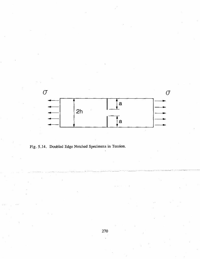
a a ' -a

'

2h -. /a '

Fig. 5.14. Doubled Edge Notched Specimens in Tension.

270

approximately valid. The double edge notched test specimen (Fig. 5.14) can be used to

develop the fracture analysis as this specimen is somewhat representative of a slab

configuration since the centerline in this symmetrical specimen does not move in the

vertical direction. The following equation is valid for w = (a/h) < 0. 7:

N(w) = 1.12 + 0.203 w - 1.197 w2 + 1.930 w3(5.30)

where the nominal stress u is the load intensity. Eqs. (5.22) and (5.23) are useful in

applying the stress field induced by climatic effects to the determination of the stress

intensity given in Eq. (5.27) by dividing the stress field into components of tensile forces

and bending moments. The finite element analysis in this study has shown that

replacement of the distributed load on a specimen in simple tension by its resultant--a

concentrated load acting along the specimen centerline--does not yield significant change

in the K1 value, particularly where the specimen length is four times the thickness. Eq.

(5.29) can be applied to pure bending loads other than that shown in Fig. 5.12(b) by

substituting u = 6M/h2• Accordingly, the shrinkage-induced stresses (Fig. 5.3) are

transformed to a tensile force and a bending moment. For instance, if H = h/2, the

resultant tensile force is h a'h/8 then Eq. (5.30) can be used in Eq. (5.27) by substituting

a = a'h/8 (the resultant force). The bending moment, M = (5/96) o'h h2, yields a =

(5/16) a'h in which Eq. (5.29) can be used for K1 Eq. (5.28) with a due to the bending

moment.

Determination of the stress intensity, as given in Eq. (5.27), can be accomplished

for a given set of climatic conditions at anticipated sawcut locations to generate sawcut

depth guidelines (Fig. 5.15). The K1 values with different notch (sawcut) depths under

temperature and shrinkage stresses are determined with Eqs. (5.29) and (5.30). Fig. 5.16

also gives the K1 values for the temperature difference t of 10 F (5.6 C), 20 F (11 C), 30

F (17 C), 40 F (22 C), and 50 F (28 C) between the pavement top and bottom, with the

same shrinkage-induced stresses.

The type of coarse aggregate is also important. When the critical stress intensity

factor K1r equals or exceeds the fracture toughness, Krr = 500 psi·in112 = 0.550 MPa·m112

(typical for river gravel concrete at an age of 12 hours), a sawcut depth of 1 inch (2.5)

cm is enough if temperature difference is not less than 20 F (11 C).

271

s = 4.6 m s = 4.6 m

r--1i-----1 . . . . .

. .. // .... .. .... ...... .... .. .. .. ;,·,;;;g1t;;di~;i ;;;;:~; ,/' .. .. . j y

.. i/ . ~~ ....... ':-''"'""'"""'"'""'"'""""""" ._,......................................... : . .' x .. ~· .............. .

transverse saw-cut /'J../1

... +

------------~-~-·_·~~=-a _______ .. ___ J h = 254 mm

Fig. 5.15. A Two-Lane Sawcut Pavement.

'cii' .....

E cO a... ~ 1.5 ............ ...... 0 ....... ()

t 11C(20F)

ctl LL >.

1 t = 5.6 C (10 F)

:t= Cl) c

IV Q) -..J w ....... Ki1 = 0.550 MPam112

c 0.5 Cl) Cl) Q) ...... .......

(f) Pavement Thickness = 25 cm (10 inches) 0-+-~~~-,--~~~-,--~~~.-~~~,-~~~,-~~--1

0 2 4 6

Sawcut Depth (in)

Fig. 5.16. Determination of Sawcut Depths.

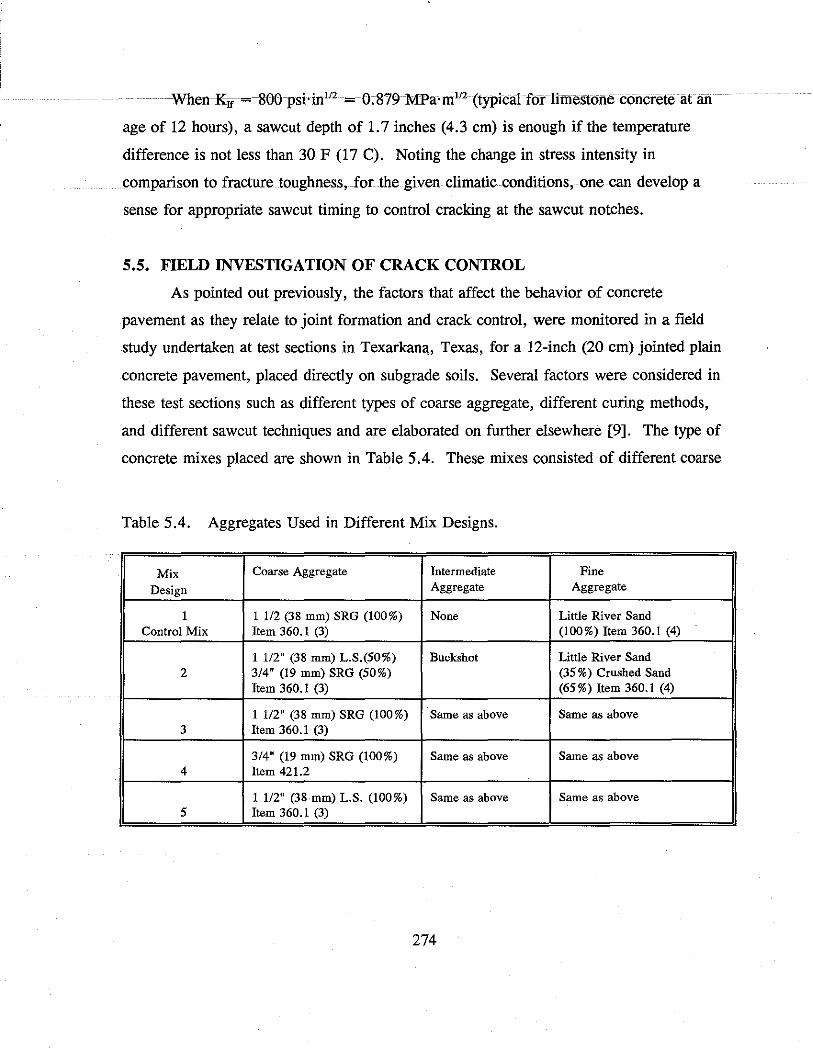
-When Krr 8()()-psi·in112 -=-0~8/9-MPa•m112 (typical for limestone concrete at an

age of 12 hours), a sawcut depth of 1. 7 inches (4.3 cm) is enough if the temperature

difference is not less than 30 F (17 C). Noting the change in stress intensity in

comparison to fracture toughness, for the given climatic conditions, one can develop a

sense for appropriate sawcut timing to control cracking at the sawcut notches.

5.5. FIELD INVESTIGATION OF CRACK CONTROL

As pointed out previously, the factors that affect the behavior of concrete

pavement as they relate to joint formation and crack control, were monitored in a field

study undertaken at test sections in Texarkan<t, Texas, for a 12-inch (20 cm) jointed plain

concrete pavement, placed directly on subgrade soils. Several factors were considered in

these test sections such as different types of coarse aggregate, different curing methods,

and different sawcut techniques and are elaborated on further elsewhere [9]. The type of

concrete mixes placed are shown in Table 5.4. These mixes consisted of different coarse

Table 5.4. Aggregates Used in Different Mix Designs.

Mix Coarse Aggregate Intermediate Fine

Design Aggregate Aggregate

1 1 1/2 (38 mm) SRG (100%) None Little River Sand Control Mix Item 360. l (3) (100%) Item 360.1 (4)

1 1/2" (38 mm) L.S.(50%) Buckshot Little River Sand 2 314" (19 mm) SRG (50%) (35 % ) Crushed Sand

Item 360.1 (3) (65%) Item 360.1 (4)

1 1/2" (38 mm) SRG (100%) Same as above Same as above 3 Item 360.1 (3)

314" (19 mm) SRG (100%) Sarne as above Same as above 4 Item 421.2

1 1/2" (38 mm) L.S. (100%) Same as above Same as above 5 Item 360.1 (3)

274

aggregate types and blends. However, some results of the-crack survey for observation

of formation of joints and cracks are provided here which coincide with calculations

previously shown. Ambient and pavement temperatures and relative humidities were

measured as indicated previously. The development of K1 and Kif are calculated and

shown in Fig. 5.17. This analysis suggests that cracking initiated 4 to 5 days after

placement. The joints in the test section pavement in Texarkana were sawcut by two

different techniques at 15 foot (4.6 m) intervals (Fig. 5.18). One method consisted of

conventional sawcut techniques using water to cool the saw blade. With this technique,

pavement was cut 3-inches (76 mm) deep (d/4). The other method consisted of early-aged

sawcut techniques. With this technique, a light and portable sawcutting machine was

used so that pavement surface notch could be placed early in the pavement life (typically

less than two to three hours after placement). Recent improvements have resulted in a

self-propelled saw shown in Fig. 5.19. This was achieved without noticeable joint

raveling. Typical sawcut depths were 1 inch_(2.5 cm) in which no cooling water was

used in the process. Crack surveys conducted from October 1991 to July 1992 (Fig. 5.20)

indicated that of all the transverse cracks which developed, only two occurred in

between the sawcut joints. These two uncontrolled cracks were initiated from the corners

of blockouts (i.e., inlet drainage structures), where stress concentration would have

existed. It is speculated that these stress-concentrations at the sharp corners could be

avoided by placing joint locations to coincide with sharp corners to guide cracking so that

uncontrolled transverse cracks would not occur.

Although the pavement test section in Texarkana was paved on November 8,

1991, (Fig. 5.20) no visible cracks were found until November 26. Cracks at the sawcut

tip were observed through the bottom of the pavement slab in later surveys. Earlier

cracks occurred at a distance from the pavement construction joint since sufficient

stresses needed to develop due to pavement restraint. It should be noted that on June 4,

1992, more joints had been formed at the early-aged sawcuts than at the conventional

sawcuts. One month later, three more cracks were found at the conventional sawcuts. A

significant amount of cracking developed after the pavement was subjected to a greater

range in temperature cycle. Since the concrete strength increased prior to the increase in

275

tv --l 0\ ,

........, ~ ..... E

"" <U Cl.. ~ ~

.... 0 0 <U u. ~ 'iii c (]) c (/) (/) Q) .... .....

(/)

1

0.8

0.6

0.4

0.2

Development of Fracture Toughness and Stress Intensity Factor

,,. .... / \ . \ . .

,,....... I \ : I ' I • J

.' \ .; \ : I • 1 1 I . \ , ' . : \! \,.,' I ' j : \ . ' • I ! ._,

• : i : ./'''· .

' I ...., : ', ; ,,,.' \ ! .....,/ ~ \ i

01+-~~~~,--~·~~~~~~~.---~~~---.~~~~~

0 1 2 3 4 5


Fig, 5.17. Development of Fracture Toughness and Stress Intensity Factor of the Sawcut.

Fracture toughness

Sirs. int let

'ti 41> l2. l2. 0 .... UI Cl c > (IJ

D..

oi 0 • "' "' N

.; Q) . "' "' N


- - "' (') 00 a) .....: lO co l.OlO

+ + + + • V lO lO IOtO '<t v '<t o::t o:t

7/.13/92 N N N N N "O

J20 ~15 ? ? J10 J5 J1 ~ : : 0 0 0 0 0 0 o : j t I I I I I I I ffi joj Cl

________ : ___ ~ __ :_ ___ :_ __ : __ ~--~---~--j ___ L __ L __ t __ L __ J __ J __ J __ J __ .:±:?_J_ _ _J_ c . I t I t I t I I I 1 I I >

i j i. <U 1--~-'-~~~~~~~~~~~~~-'-~~--11---J-~-+-~-l---11---J-~-t-~-1---11---J...~..L-...J D..

6/4/92 6/4/92 ~I/ 6/4/92

11/26/91

( 1/8" Wide, 2/20/92)

11/26/91

( 1/8" Wide, 2/20/92)

11/26/91 2/20/92

( 1/8" wide, 2/20/92) ( 118" wide, 2/20/92)


Coventlonal sawcut

Early-aged sawcut

(Tee blade)

Fig. 5.18. Layout of a Test Section.



(Tee blade)

'

Fig. 5.19. Soft-Cut Early Sawcutting Machine.

278

Mix Design 2 The section was paved on Nov. 8, 1991

90

80

Ol 70 c

:52 60 u cu .._

50 0 -0 40 IV .....

-.J c \{) Cll

u 30 .._ Cll a.. 20

10

0 Nov. 26 Feb.20 Jun.4 Jul. 13

Date after Paving

CJ Conventional Sawcut m Early Aged Sawcut

Fig. 5.20. Cracking Development.

cracking, it is speculated that cracking at the sawcuts, although observed much later after

construction, initiated early in the life of the pavement which may be indicative that a

certain level of damage is necessary to insure that cracking will occur at the sawcut joint.

A closer look at the evolution of cracking can be taken by examining the results shown in

Fig. 5.8. The initial crack interval was on the order of 90 feet (27.4 m) or more.

Apparently, it is intervals of this magnitude where the combination of curl, warping, and

frictional stresses was enough to initiate cracking (Fig. 5.17). The frictional stress may

have been the significant contribution to crack development given the climatic conditions

under which the paving was accomplished although a much improved crack pattern

developed the following summer. The disadvantage of a crack pattern developing in this

manner is that some joints open wider than designed, which may damage the joint sealant

material. It should be pointed out that this characteristic was prevalent whether

conventional or early-aged cutting techniques were used. This condition may be

minimized by using a jointed reinforced concrete pavement type.

It is interesting to note that different types of aggregate affect the fracture

properties and crack development of concrete pavement as shown in Fig. 5.21. Cracking

at the sawcut tip occurred more frequently where the concrete coarse aggregate type was

river gravel rather than crushed limestone concrete. This was also the case in the

subsection paved with the concrete that used a blend of crushed limestone and river

gravel as the coarse aggregate in comparison to that paved with the concrete that used

crushed limestone only as the coarse aggregate. Lab tests showed that concrete of

crushed limestone had higher flexural and compressive strengths than concrete of river

gravel at early ages [11, 19]. These field results tend to confirm the validity of using

early-aged sawcutting techniques. Although not expressly addressed in this paper, it

appears that sawcut timing is much more significant than sawcut depth. A shallow notch

placed early in the pavement surface can take advantage of the greater change in

temperature and moisture in the vicinity of the pavement surface (in comparison with the

changes occuring at a greater depth) which results in a greater amount of crack damage

and subsequent incidence of cracking at the notches.

280

N 00 -

Percentage of Cracked Sawcuts (%) 120

100

80

60

40

20

0 Mix 3 (10/14) Mix 1 (10/16) Mix 5 (10/18) Mix 4 (10/22) Mix 5 (11/6)

Test Section

~ 11110191 D 2120192 • 6/4/92 D 7/13/92

••••

.·.·

••••

Mix 2 (11/8)

Fig. 5.21. Percentage of the Sawcuts Having Cracked Observed at Different Dates in Test Sections Paved at Different· Dates (Dates in Parentheses) with Different Concrete Mix Designs.

5.6. CONCLUSIONS

Modified linear fracture mechanics is applicable in determining sawcut depth for

early cracks. The sawcut depth is dependent on the spacing of the transverse sawcut, the

material fracture parameters K1, and Cr, and the stress level in the concrete slab with

given geometrical conditions. The material fracture parameters vary with time, especially

at early ages of concrete. Field observation has found that late cracks are also initiated by

the sawcutting notches. However, the propagation of these cracks may be caused by long

term fluctuating thermal and moisture loads, for which further research is needed.

The reduction of sawcut depth (less than d/3 or d/4) at concrete joints by early-aged

sawcut or placement techniques will take advantage of the greater change in moisture and

temperature in the concrete at the pavement surface (in comparison to the change at d/3

or d/4) to initiate cracking at the notches at a greater incidence than otherwise.

Therefore, the control of concrete pavement cracking should be improved. Field surveys

indicate that under some circumstances (such as cool weather paving conditions)

transverse cracks at, the sawcut notches may initiate much later after placement. On a

preliminary basis, this study indicates that it is reasonable to use notch depths on the

order of 1 inch (2.5 cm), to initiate cracking at the pavement surface, which is

significantly less than the traditional d/4 or d/3.

5.7. APPENDIX: REFERENCES

I. Emborg, M., "Thermal Stresses in Concrete Structures at Early Ages," Doctoral

Thesis, Luleii University of Technology, Luleii, Germany, 1989.

2. Richardson, J.M., and Armaghani, J.M., "Stress Caused by Temperature Gradient

in Portland Cement Concrete Pavements," Transportation Research Record 1121,

1987, pp. 7-13. Transportation Research Board, Washington, D. C., 1987.

3. Westergaard, H. M., "Analysis of Stresses in Concrete Pavements Due to Variations

of Temperature," Proceedings of the Sixth Annual Meeting, Highway Research

Board, 1927, pp. 201-205.

4. Bradbury, R. D., "Reinforced Concrete Pavements," Wire Reinforcement Institute,

Washington, D. C., 1938, pp. 34-41.

282

5. Tang, T., and Zollinger, D.G., and Senadheera, S, "Analysis of Concrete Curling in

Concrete Slabs," Journal of Transportation Engineering, V. 119, No. 4, July/August

1993, pp. 618-633.

6. Ba.Zant, Z. P., and Wu, S. T., "Creep and Shrinkage Law for Concrete at Variable

Humidity," Journal of tbe Engineering Mechanics Division, Vol. 100, No. 1974, pp.

1183-1209.

7. Bafant, Z. P., and Panula, L., "Practical Prediction of Time-Dependent Deformation

of Concrete. Part 3: Drying Creep. Part 4: Temperature Effect on Basic Creep,"

Materiaux et Constructions, Vol. 11, No. 66, 1978, pp. 415-424.

8. Buch, Neeraj and Zollinger, D.G., "Preliminary Investigation on tbe Effect of

Moisture on Concrete Pavement Strengtb and Behavior," A paper prepared for tbe

72nd Annual Meeting of the Transportation Research Board, 1993.

9. Tang, T., Zollinger, D.G., and McCullough, Frank, "Texarkana Test Sections,"

Technical Memorandum, Research Project 1244, February 1993.

10. Yoder, E.J. and Witczak, M.W., (1975), Principles of Pavement Design, 2nd

Edition, John Wiley and Sons.

11. McCullough, B. Frank, "Mechanistic Analysis of Continuously Reinforced Concrete

Pavements Considering Material Characteristics, Variability, and Fatigue," Research

Report 1169-2, Center for Transportation Research, tbe University of Texas at

Austin, April 1990.

12. Palmer, R.P., Olsen, M., and Lytton, R.L., "TTICRCP - A Mechanistic model for

tbe Prediction of Stresses, Strains,and Displacements in Continuously Reinforced

Concrete Pavements," Research Report 371-2F, Texas Transportation Institute,

Texas A&M University, August 1987.

13. Grzybowski, M., "Determination of Crack Arresting Properties of Fiber Reinforced

Cementitious Composites," Royal Institute of Technology, Stockholm, Sweden,

1989.

14. England, G. L., and Illston, J. M., "Metbods of Computing Stress in Concrete from

a History of Measured Strain," Civil Engineering and Public Works Review, Vol.

60, 1965: April - pp. 513-717; May - pp. 692-694; and June - pp. 846-847.

283

Documents

Field Tests and Analyses of Concrete Pavement in Texarkana ... · FIELD TESTS AND ANALYSES OF CONCRETE PAVEMENT May 1994 IN TEXARKANA AND LA PORTE, TEXAS 6. Performing Organization