Embed Size (px)
Citation preview

Field Measurement and Evaluation of Time-Dependent Losses in Prestressed Concrete Bridges
Project Number: WPI-0510735
Draft Final Report
submitted to
Florida Department' of Transportation
Dr. Moussa Issa, P.M.
by Dr. Okey Onyemelukwe, P.L Dr. Sashi Kunnath, Co-P.I.
University of Central Florida
Orlando, Florida 32816
February 24, 1997


ii

iii

LIST OF TABLES
2-1 Properties for Standard and Modified Type VI Girders............................... 21
2-2 Detailed information about composite slab gauges...................................... 31
2-3 Experimental results of E,. and f.' ............................................................... 48
2-4 28 day strength for girders.......................................................................... 51
2-5 Design E,,(t) versus CEB-FIP E,(t) ............................................................. 52
3-1 AASHTO lump sum time-dependent equations........................................... 59
3-2 Values of K,.e and J ..................................................................................... 67
3-3 Values of C ................................................................................................ 68
3-4 Spreadsheet results for midspan.................................................................. 69
3-5 Spreadsheet results for other locations........................................................ 70
4-1 Examples of the raw collected data............................................................. 73
5-1 Limitations on strand stress ....................................................................... 128
5-2 Resulting tendon stresses............................................................................ 129
5-3 Allowable concrete stresses........................................................................ 131
5-4 Camber and deflection readings .................................................................151
A-1 ACI Committe 209 E,(t) versus Design E,-(t)............................................ 155
iv

LIST OF FIGURES
2-1 Bridge configuration .................................................................................. 19
2-2 Bridge cross-section.................................................................................... 19
2-3 Standard and Modified AASHTO Type VI................................................. 21
2-4 Ends and Midspan cross-section with tendons ............................................21
2-5 Tendon profile ......................................................................................…... 22
2-6 Vibrating wire strain gauge......................................................................... 23
2-7 Instrumented locations ............................................................................... 26
2-8 Midspan gauge distribution ........................................................................ 27
2-9 Quarter-span gauge distribution.................................................................. 29
2-10 1.52 m gauge distribution ............................. ......... .................. ................ 29
2-11 Slab gauge distribution............................................................................….31
2-12a Preparation of strain gauges ....................................................................... 34 .
2-12b Placement of strain gauges ..........................,.............................................. 35
2-12c Attachment of strain gauges ....................................................................... 36
2-12d Instrumented girder awaiting shipping ........................................................ 37
2-13 Bridge cross-section with equipment .......................................................... 39
2-14a Placement of girder and reinforcement........................................................ 41
2-14b Multiplexers attached to girder.................................................................42
v

2-14c Other equipment at bridge site..................................................................… 43
2-15a Preparation of shrinkage cylinders ..........................................................….. 44
2-15b Shrinkage cylinders at bridge site............................................................….. 45
4-1 Unfiltered strain and internal temperature data........................................….. 73
4-2 Unfiltered ambient temperature and relative humidity ................................. 74
4-3 Relative humidity and ambient temperature for Beams 1 and 4.................... 79
4-4 Relative humidity and ambient temperature for Beams 2 and 3.................... 79
4-5 Elastic shortening Beam 1 Midspan ..........................................................… 81
4-6 Elastic shortening Beam 4 Midspan .........................................................…. 81
4-7 Elastic shortening Beam 3 Midspan .........................................................…. 82
4-8 Average elastic shortening for midspans .................................................….. 83
4-9 Elastic shortening Beam 3 Quarter-span ................................................…... 84
4-10 Elastic shortening 1.52 m Beam 1..........................................................…... 84
4-11 Elastic shortening 1.52 m Beam 4..........................................................….... 85
4-12 Average elastic shortening for 1.52 m......................................................…. 86
4-13 Elastic shortening variation with length .................................................…... 87
4-14 Time-dependent prestress loss Beam 1 Midspan ........................................... 89
4-15 Time-dependent prestress loss Beam.4 Midspan .....................................….. 89
4-16 Time-dependent prestress loss Beam.3 Midspan .......................................… 90
4-17 Average time-dependent prestress loss for midspans.................................… 90
4-18 Time-dependent prestress loss Beam 3 Quarter-span ................................… 92
4-19 Time-dependent prestress loss 1.52 m Beam 1........................................….. 92
Vi

4-20 Time-dependent prestress loss 1.52 m Beam 4............................................ ..93
4-21 Average time-dependent prestress loss for 1.52 m ...............................…..... .93
4-22 Time-dependent prestress loss with length ..........................................…...... .94
4-23 Lump sum prestress loss Beam 1 Midspan.........................................….....… 96
4-24 Lump sum prestress loss Beam 4 Midspan..........................................…....… 96
4-25 Lump sum prestress loss Beam 3 Midspan.............................................….… 97
4-26 Average lump sum prestress loss for midspans......................................….... .97
4-27 Lump sum prestress loss Beam 3 Quarter-span......................................…... ..98
4-28 Lump sum prestress loss 1.52 m Beam 1 ............................................…....… 98
4-29 Lump sum prestress loss 1.52 m Beam 4 ...........................................…....... ..99
4-30 Average lump sum prestress loss for 1.52 m..........................................….… 99
4-31 Lump sum prestress loss with length...........................................................…101
5-la-b Cross-sectional loss variation Beam 1 Midspan.......................................……105
5-lc-d Cross-sectional loss variation Beam 1 Midspan.........................................…..106
5-2a-b Cross-sectional loss variation Beam 3 Quarter-span................................….. 108
5-2c-d Cross-sectional loss variation Beam 3 Quarter-span................................….. 109
5-3a-b Cross-sectional loss variation 1.52 m Beam 4... ....................................….... 111
5-3c-d Cross-sectional loss variation 1.52 m Beam 4 ..........................................…. 112
5-4 fpi / fp; for Midspan Beam 1..................................................................…...... 116
5-5 fpi / fpj for Quarter-span Beam 3 ...........................................................…..... 116
5-6 fpi I fpj for 1.52 m Beam 4 ....................................................................…...... 117
5-7a-b R and 1-R for Midspan Beam 1 .............................................................….... 120
vii

5-8a-b R and 1-R for Quarter-span Beam 3 .........................................................….121
5-9a-b R and 1-R for 1.52 m Beam 3...................................................................…..122
5-10 Lump sum loss to jacking stress ratio for NEdspan Beam 1......................... 125
5-11 Lump sum loss to jacking stress ratio for Quarter-span Beam 3 .................. 125
5-12 Lump sum loss to jacking stress ratio for 1.52 m Beam 4............................ 125
5-13 NEdspan Beam 1 at transfer......................................................................….135
5-14 NEdspan Beam 1 at transfer......................................................................….135
5-15 Quarter-span Beam 3 at transfer...............................................................…..136
5-16 Quarter-span Beam 3 at transfer.............................................................…... 136
5-17 1.52 m Beam 4 at transfer .............................................................…............ 137
5-18 1.52 m Beam 4 at transfer ..................................................................…....... 137
5-19 Relative Humidity versus Loss Midspan Beam 1.......................................... 141
5-20 Relative Humidity versus Loss NEdspan Beam 3......................................... 142
5-21 Relative Humidity versus Loss Quarter-span Beam 3 .................................. 143
5-22 Relative Humidity versus Loss 1.52 m Beam 4 ........................................... 144
5-23 Ambient Temperature versus Loss NEdspan Beam 1................................... 146
5-24 Ambient Temperature versus Loss Midspan Beam 3 ................................... 147
5-25 Ambient Temperature versus Loss Quarter-span Beam 3 ............................ 148
5-26 Ambient Temperature versus Loss 1.52 m Beam 4 ...................................... 149
5-27 Camber for Midspan of Beams 1, 4, and 3 ................................................... 153
viii

CHAPTER 1
INTRODUCTION
1.1 Background
The Florida Department of Transportation (FDOT) is frequently confronted with
contractor suggested redesigns of some of its prestressed concrete bridge projects. In
which case most of the contractors call for changing the bridge girder design from its
original post-tensioned continuous members to longer simple supported spans. Often,
these result in deeper simple span girders with larger cross-sectional areas, moment of
inertia and consequently, greater ultimate capacity. Thus, enabling the designer to
eliminate the post-tensioning and change the statical scheme from continuous to simply
supported.
Therefore, although the girders are designed as simple spans, the attached deck
slabs remain as continuous members. The final configuration of both the deck slab and the
girder acting as a unit, is in essence a hybrid between a strictly statically indeterminate
structure and a determinate structure. Further investigation of this sort of design is
necessary, since the time-dependent behavior of these members with respect to creep,
t

shrinkage and steel relaxation is drastically different for indeterminate structures when
compared to simple ones.
Therefore, it is the objective in this project to conduct the following studies:
Instrument sections of the bridge girder and deck slab for strain and temperature
measurements, which will be used in determining the prestress losses in the members
Utilize the field measured data to determine the effects of the relative shrinkage
between the continuous slab and the simply supported beam.
Reduce and process the measured data to form a useful database for future use by
MOT in related projects
Use analytical and code procedures for prestressed concrete bridge design to establish
the adequacy or ramifications of the modified design. Especially, since most of these
redesigns claim the simply supported system has the same structural capabilities as
the continuous post-tensioned design, and that both designs should be considered
equivalent.
In this report the effects of time-dependent prestress losses in prestressed concrete
bridges are studied. Time-dependent behavior of concrete is an important consideration in
11

the design and analysis of structures, especially with respect to prestressed concrete
bridges. Both prestressed concrete and conventional reinforced concrete tend to deform
with time. The reasons for these continuous deformations include creep and shrinkage.
These deformations directly affect the strains in the concrete, which also change with time.
Therefore, creep and shrinkage must be compensated for before a member can perform at
its best. Without accounting for creep and shrinkage effects, serviceability problems may
arise with excessive camber, deflection, and/or flexural stresses. The change in stress due
to the above mentioned phenomena are classified as part of the prestress losses, and must
be accounted for in the design of prestressed concrete members.
There are two categories of prestress loss: instantaneous losses and timedependent
losses. The instantaneous prestress losses are made up primarily of anchorage slip, friction,
and elastic shortening. These losses occur only once and do not necessarily vary with time.
The time-dependent losses consist of creep and shrinkage of concrete and relaxation of the
prestressing steel. These losses vary throughout the lifetime of a member and increase
rapidly at the early age of the concrete, while increase over the remaining life occurs at a
decreasing rate.
Prestress losses are often accounted for by two different approaches. One method
takes a known lump sum value established from similar members as the prestress loss for
the member being examined. In this approach, the prestressed loss is often expressed as a
percentage of the initial stress applied to the steel strands. The other method involves
calculating each contribution of the loss separately, summing these components and taking
12

that sum as the total prestress loss. In the sections that follow, a general overview of
prestressing of concrete structures will be presented. After which, more specific details as
they apply to the Westbound Gandy Bridge project will be covered.
1.2 Methods for Prestressing Concrete
Prestressed concrete involves the pre-application of compressive force, transferred
from the steel tendons, to the surrounding concrete. This compressive load, which is
typically eccentric, is designed to counteract the service load that will be applied on the
member during its lifetime. Upon application of this prestress force, the beam will bow
concave upward from the casting bed and rest on its ends. This bowing action caused by
the preloading is referred to as camber or "negative deflection." The stress distribution
resulting from the prestress force would consist of tensile stresses toward the top of the
member and compressive stresses toward its bottom. As the service loads are applied the
member tends to deform downward or deflect, overcoming the initial camber. This results
in the member being mainly kept in compression toward its top, and with little or no
tensile stresses near the bottom. Since concrete is much stronger in compression than it is
in tension, it would be beneficial to keep the member in as much compression as possible.
This is precisely what prestressing does, it virtually eliminates tensile stresses that would
otherwise occur under service load conditions.
4

Prestressed concrete offers many advantages over conventional reinforced concrete.
For example, prestressed concrete allows for the use of stronger materials, such as high-
strength steel (with yield strengths of 18621VIPa (270 ksi)) and high-strength concrete
(with compressive strengths of 34.5 MPa (5 ksi) and above). These materials cannot be
used with conventional reinforced concrete because their properties are not consistent with
that type of design. The higher strength concrete and steel allow for smaller and lighter
sections, than those used for conventional reinforced concrete members with the same load
carrying capacity. Cracking, deflections, and service load stresses can be controlled easily
using these high-strength materials with prestressed concrete.
It is theoretically possible to design a member with zero tensile stress and such a
case is known as full prestressing. This case is very limiting and often leads to troublesome
excessive camber after loads are applied. This excessive camber in flexural prestressed
members can create uneven driving surfaces in bridges, or promote cracking in walls of
buildings as well as other problems. These problems have lead to a viable alternative to full
prestressing known as partial prestressing. Lying somewhere between both conventional
reinforced concrete and full prestressing is partial prestressing. This midway alternative
requires the use of conventional steel reinforcement in addition to prestressing steel,
depending on the design, to provide additional load carrying capacity. Quite often the non-
prestressed steel is also used to control the crack width that develops in the member.
Prestressed concrete is used in many different types of structures such as bridges,
parking garages, and floor beams in buildings to name a few. The advantages of
14

prestressed concrete are vast, which explains why the use of this form of construction has
continued to increase throughout the years.
There are two methods used to induce a compressive load on a prestressed concrete
member. These methods are pretensioning and post-tensioning. The basic idea of
pretensioning is that the steel strands are tensioned before the concrete is cast around them.
With post-tensioning, the steel strands are not tensioned until after the concrete has been
casted. A brief discussion of these two methods will now be presented.
1.2.1 Pretensioning
Pretensioning consists of prestressing the tendons before the concrete is casted
around it. In order to achieve this, it is necessary to attach the ends of the prestressing
strands to permanent abutments. Then at one abutment a jack is used to tension the strands
against the other abutment. After the concrete is casted and achieves sufficient strength, the
strands are then cut from the abutments allowing the prestress to be transferred to the
concrete. This stress is transferred through the bond between the concrete and the
prestressing steel. Some advantages to pretensioning are the ability to produce many beams
within a shorter period of time and under controlled conditions. A specific method for
pretensioning concrete is the long'-line method. This method prestresses strands for many
members which will be casted end-to-end along a single bed. This economical method
saves on labor costs and allows for reusable forms.
15

Pretensioning is the method predominantly used for prestressing concrete in the industry
today.
1.2.2 Post-tensioning
Post-tensioning involves casting concrete around conduits which contain
unstressed steel. After the concrete reaches a specified strength these strands are then
tensioned, usually at the construction site. The beam is prepared with a special anchorage
system at one end which allows it to be tensioned against itself. Quite often multiple
beams are post-tensioned at the same time to form one continuous member. In this case
the conduits are left empty during casting and the strands are shot through just before
tensioning. Post-tensioning is usually done in the field. After the strands are tensioned,
grout is then pumped into the conduits filling any voids that may be present. An
advantage of post-tensioning is that the conduits can be easily shaped to allow for many
different types of tendon profiles. Post-tensioning also allows for the combination of
single members to form one continuous unit. This is achieved by passing the steel tendons
through the ducts of each of the members and tensioning the strands, thus causing these
members to act as one. l
Pretensioning and post-tensioning of prestressed concrete offer many different
alternatives to the designer. In most situations, the design itself will dictate which of these
options is more viable.
16

1.3 Prestress Losses
1.3.1 Introduction
In our discussion so far about prestressed concrete there has been little detail on
the variation of prestress force during the lifetime of the member. This is important
because the constant prestressing force first applied does not remain constant during the
lifetime of the structure. The loss of prestress, which is broken down into instantaneous
and time-dependent losses, accounts for this variation in force and stress in the strand.
The instantaneous prestress loss represent losses felt just before or immediately after the
transfer of the prestressing force to the concrete. Conversely, the time-dependent
prestress losses are those that are constantly varying throughout the lifetime of the
member. It is important to accurately account for both of these types of losses. Failure to
do so will affect serviceability conditions more so than the ultimate capacity of the
member. Camber, deflection, and cracking are examples of service conditions that can be
affected by incorrectly computing the prestress losses. Such errors would have little
effect on the ultimate strength of a flexural member unless the steel tendons are
unbonded or if their final stress after losses is less than 0.5fpu, where fpu, is equal to the
ultimate strength of the prestressing strand.2
17

1.3.2 Instantaneous Losses
The instantaneous prestress loss which occurs just before, or at transfer of
prestress from the strands to the concrete consists of three main constituents: frictional
losses, anchorage slip, and elastic shortening of the concrete. Depending on the method
of prestressing being used some of these losses may not be applicable. A brief
description of these losses and when they apply follows.
1.3.2.1 Anchorage Seating Loss and Frictional Losses
Upon transfer of the prestress force to the anchorage seat, some slippage is
caused due to the deformation of the connection holding the steel strands. This causes
the stressed tendons to loosen and lose some stress. Typically the anchorage slip can be
compensated for by overstressing the steel strands. Anchorage slip is typically
applicable to post-tensioning although in pretensioning a comparable condition occurs
with the connections at the abutment.
The loss of prestress due to friction occurs between the steel tendons and its duct
or ducts. Hence, this type of loss is often associated with post-tensioning. The loss is
comprised of two parts: the wobble effect and the curvature effect. These effects deal
with the friction due to the misalignment of the ducts, and accidental curvature of the
steel tendons, respectively. The frictional loss varies with the length of the member. The
frictional loss can also be compensated for by overstressing the tendons. In general,
18

frictional losses only apply to post-tensioned members and are often neglected for
pretensioned members because its effect is usually very small.'
Anchorage seat and friction loss are mechanical types of loss. These losses are the
difference between the jacking load and the applied load. The anchorage seat and frictional
losses can be calculated and either partially or fully compensated for by overstressing.4
1.3.2.2 Elastic Shortening
Elastic shortening of concrete deals directly with the relationship between the
prestressing steel strands, and the surrounding concrete which is bonded to it. The transfer
of the prestressing force to the steel strands causes them to shorten, which in turn causes
the bonded concrete to shorten as well. Elastic shortening is usually calculated at the
prestressing steel centroid and is accounted for differently depending on the method of
prestressing used.
For a pretensioned member, elastic shortening usually varies with length with a
maximum occurring at the midspan. In post-tensioned members, the loss is dependent
upon whether the strands are all tensioned at the same time or in a sequential order. If the
strands are all tensioned at once, there is no loss from elastic shortening. On the other
hand, if the strands are stressed at different times elastic shortening loss will occur and
must be accounted for.
19

These instantaneous losses, made up of anchorage slip, friction, and elastic
shortening, reduce the jacking stress and subsequent force to some lower value. The
reduced force is often referred to as the initial prestress force. This force will be considered
the actual force applied to the member. However, the initial prestress force does not remain
constant, it will be reduced by the time-dependent prestress losses.
1.3.3 Time-Dependent Prestress Losses
The prestressing force is continually changing throughout the lifetime of a
structure. This change is not only because of the variation of service loads, but because of
the time-dependent prestress losses. These losses, as their name suggests, are time
variant. As time proceeds the rate of increase of these losses continues at a decreasing rate.
The time-dependent losses are primarily made up of three components. These are creep and
shrinkage of the concrete, and relaxation of the prestressing steel after its application to the
concrete. It is very difficult to determine each individual contribution of these losses to the
time-dependent loss as a whole because they are all inter-related. Hence, a variation in one
directly causes a change in the others and vice-versa.
1.3.3.1 Creep
Creep is the continual straining of concrete under sustained loading for a period of
time. The phenomenon of creep is not only a problem for prestressed concrete, but for all
types of concrete members that have a constant load for a duration of time. This excess
II

deformation due to creep is caused in addition to the immediate elastic straining created by
the application of the load. As time of loading increases the effect of creep gradually
diminishes. These creep strains created are usually more significant than the elastic strains.
Unlike elastic strains, only a portion of the creep strains are recoverable.
The creep of concrete due to the prestress in turn reduces the stress in the steel,
which causes prestress loss. Creep is directly effected by the shrinkage of concrete and the
relaxation of the steel, both which will be explained later. These three time-dependent
mechanisms are inter-related and work together to create prestress loss over time.'
Creep is influenced by many factors. Some of these factors include; amount and
duration of sustained loading, age at time of loading, water-to-cement ratio of the concrete
mixture, aggregate modulus of elasticity and aggregate-paste ratios, the size of the concrete
member, and amount of steel reinforcement present. Most of these effects would be
considered in determining the prestress losses in the Gandy Bridge Project.
1.3.3.2 Shrinkage
Shrinkage is the time-varying loss of excess water in a concrete member. Like
creep, shrinkage is not just a problem for prestressed members but all concrete members in
general. When the concrete for a member is poured it usually contains water above what
is necessary for chemical hydration of the cement to enhance its workability. This excess
water slowly evaporates throughout time.
21

Shrinkage causes the member to shorten, which in turn leads to loss of some stress
in the prestressed steel tendons. If a member was totally immersed in a 100 percent
relative humidity environment over its life, there would be no shrinkage loss. But since
such a condition is highly irregular over the life of a member, shrinkage must be
accounted for.
Shrinkage of concrete is affected by many different factors. Some of these factors
include the materials used in the concrete design and mix. These include; the type of
aggregate used, the water-to-cement ratio, the type of admixtures and cement used. The
physical properties of the member may also affect the amount and rate of shrinkage
occurring. The strength of the concrete used, the amount of steel reinforcement used, and
the volume-to-surface area ratio are some of these physical properties. The existing
environmental conditions such as ambient temperature and relative humidity play a part
in determining the shrinkage that will occur.
1.3.3.3 Steel Relaxation
Steel relaxation is the decrease of stress in a tendon while the length remains
relatively constant. This differs from creep of concrete, which is change in strain under a
constant stress. The tendon length is assumed constant when considering the prestress
loss from steel relaxation. In reality this is not the case, the length is affected by the other
time-dependents losses, namely creep and shrinkage of the concrete a well as changes in
the applied loads.
22

Steel relaxation is not the only loss that affects the stress in the steel tendons. Elastic
shortening, creep, and shrinkage of the concrete also change the stress in the prestressing
steel. This inter-dependence between the steel relaxation, elastic shortening, and the other
time-dependent losses further complicates the calculations of the individual components
of the total loss.
There are a few conditions that influence steel relaxation. The amount of prestress
applied to the steel tendons, the type and strength of the tendons used, and the time the
stress was applied are the primary conditions of importance. Another factor that is
considered in accounting for the loss due to steel relaxation is the method of prestressing
used to tension the member. For pretensioned members, there is steel relaxation
occurring before the strands are applied to the concrete as well as after. The steel
relaxation for these two time periods are accounted for differently. For post-tensioned
members, the steel relaxation loss begins immediately after the strands are stressed
against the concrete.
As described in the previous paragraphs, the time-dependent losses, namely creep
and shrinkage of concrete and steel relaxation, are difficult to account for individually
since they are all inter-related. However, these time-dependent losses all continue
through time at a decreasing rate. Neglecting these losses may not lead to catastrophic
failure, but would directly influence serviceability conditions.
23

1.4 Westbound Gandy Bridge Project
This report studies the effects of time-dependent prestress losses in prestressed
concrete girders by instrumenting an actual bridge. Strain measurements, taken from these
girders, are used to deduce the actual prestress loss. The strain readings were obtained by
using embedded vibrating wire strain gauges.
The Westbound Gandy Bridge in Pinellas and Hillsborough Counties of Florida,
is the actual bridge used in this case study. The original design for the Approach span
consisted of 25 typical units made up primarily of 4-span continuous post-tensioned
girders of 144 ft. The re-design consists of 31 typical units made up primarily of 3-simply
supported spans of 144 ft. The new bridge configuration is primarily composed of 43.9
meter (144 foot) pretensioned modified AASHTO Type VI concrete girders. According to
the Value Engineering Report', this girder is 15.25 cm (6 inches) deeper than the Florida
Bulb-T, and has 18% additional area, but a 44% greater moment of inertia and 64% greater
ultimate capacity. These girders are set on the bridge as three span simply supported units.
Composite action is then achieved with a continuous slab over these spans. This hybrid
structural configuration is lacking in performance data, especially with respect to prestress
losses, camber, and deflection. To investigate these conditions four strategically located
girders were chosen for instrumentation in this project. Three locations along the span were
picked for the placement of a series of gauges. These points are at the midspan, quarter-
span and 1.52 meters (5 feet) from the end support.
24

Therefore, all instrumented girders have gauges at their midspans as well as gauges at
either the quarter-span or 1.52 meters (5 feet) from the end support.
At each of the location selected along the span, series of gauges were placed
throughout the cross-section. Some of the cross-sectional points chosen had physical
significance, such as the steel, concrete, and composite section centroids. Additional
points between those already mentioned were picked to account for the variation between
them.
Data collection began in December 1995 at the Hardaway Prestress Plant in
Tampa, Florida, where the beams were casted. The beams were placed at the bridge site in
April 1996 by Misener Marine Construction Company, where data collection is still on
going, and is currently scheduled to continue for another two years.
This report will deal with the data collected from the studied beams just after they
were cast and stressed, through their placement upon the bridge, and before the composite
slab was poured. The data from this period in all covers 150 days.
The format and content of the rest of the body of this report is presented next.
Chapter 2, Girder and Bridge Instrumentation, entails all instrumentation aspects of the
girder and bridge studied, what equipment was used and how it was installed, what gauge
locations were chosen and why, and other important experimental details. Chapter 3, Code
Treatment of Prestress Losses, illustrates how various Codes treat prestress losses.
Chapter 4, Data Analysis and Experimental Results, explains how results were obtained,
separates the immediate losses from the time-dependent losses, contains various plots of
25

prestress loss, and compares Code results with those obtained. Chapter 5, Effects of
Prestress Loss on Bridge Design, examines the effects of prestress losses within the
girder cross-sections, utilizes percent comparison with Codes, calculates tendon and
concrete stresses, investigates the relationship of relative humidity and ambient
temperature with prestress losses, and compares actual camber readings to those
calculated using the prestress loss of Chapter 4.
1.5 Unit Conversion
The calculations done throughout this research report were done using the
English system of units such as feet, pounds, and ksi. The final results were than
converted into the SI system of units, centimeters, Newton, and Mega-Pascal. The three
primary conversion factors used throughout this report are as follows:
1 in = 2.54 cm
1 lb = 4.448 N
1 ksi = 6.895 MPa
The dimensions and results are reported in SI units, with the English equivalent
occurring in parentheses. It is important to note that calculations were done in English
system of units and then converted to SI units, although the SI units are presented as the
primary unit.
17

CHAPTER 2
GIRDER AND BRIDGE INSTRUMENTATION
2.1 Introduction
The Westbound Gandy Bridge is made up of many different span lengths, of
which the most frequent occurring span length is 43.9 m (144 feet). Since this length is
most prevalent, girders this length were selected for this study. Each of these 43.9 meter
(144 foot) girders have the shape of the AASHTO Type VI girder with some
modifications. Four of these Modified AASHTO Type VI girders were selected for
instrumentation in this project.
2.1.1 Bridge Configuration
The design of the bridge calls for three simply-supported pretensioned girders with
a continuous reinforced concrete deck, to form composite action over the three spans. A
typical cross-section of the bridge consists of four girders, two of which are interior, and
two of which are exterior. This bridge configuration and typical cross-section can be seen
in Figure 2-1 and 2-2, respectively. In order to see the variation of the loading effects after
the slab is casted, for the interior spans versus the exterior spans, two of each type were
chosen for instrumentation. These four girders are representative of the entire three
18
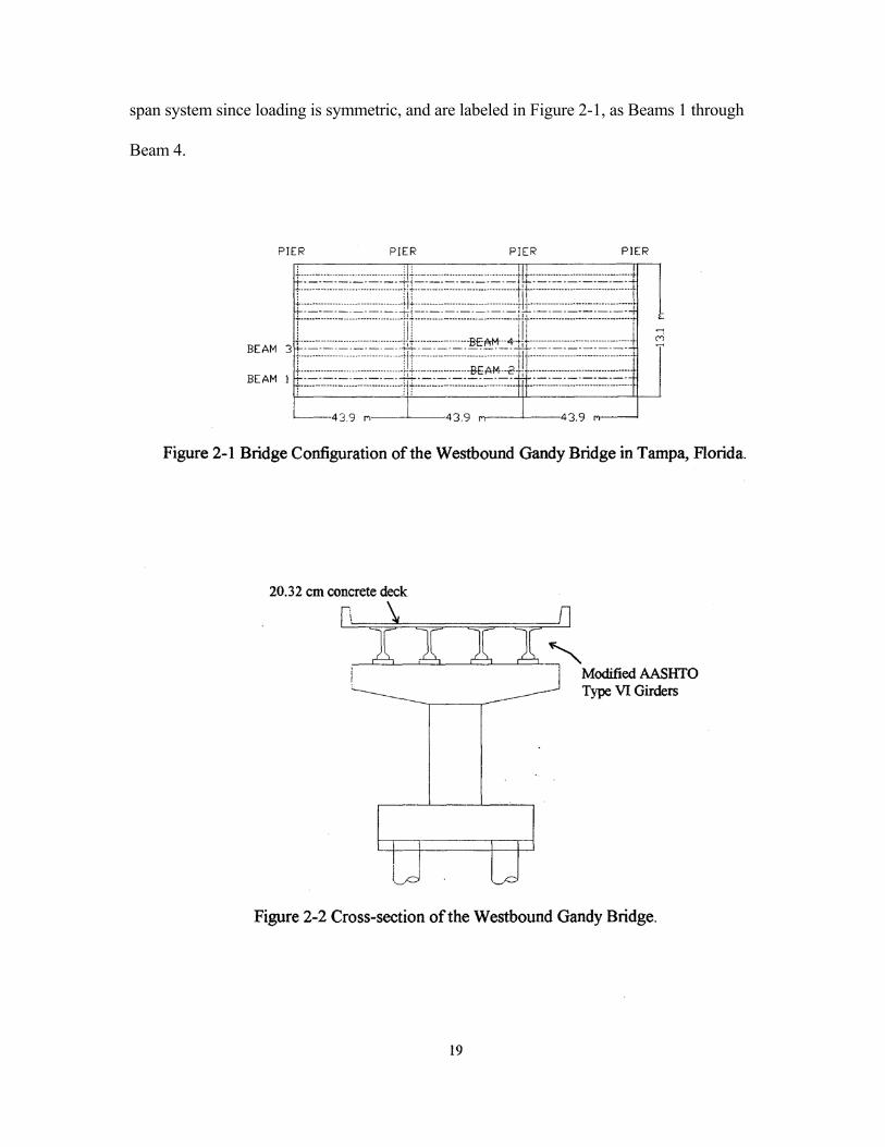
span system since loading is symmetric, and are labeled in Figure 2-1, as Beams 1 through
Beam 4.

2.1.2 Modified AASHTO Type VI
As mentioned earlier, the girder type investigated in this project is the Modified
AASHTO Type VI. This girder is derived from the Standard Type VI Bridge Girders suggested
by AASHTO. In Figure 2-3 both the Standard AASHTO and the Modified AASHTO Type VI
girders are presented with their properties in Table 2-1. The Modified Type VI is 15.2 cm (6 in)
taller, and has a maximum top flange width 47.5 cm (18 in) wider, when compared to that of the
Standard Type VI as well as other dimensional changes. These changes allow for an increase in
the gross moment of inertia of the section, I., of 21 % while only increasing the self weight of the
member by less than 2 %.
The design of the Modified AASHTO Type VI girder used on the Westbound Gandy
Bridge consists of, 64 - 1.27 cm (1/2 inch) oversized or special 1862 MPa (270 ksi -seven-wire
low relaxation prestressing strands pulled at 150.3 IN (33.8 kips) each. These 1.27 cm (i/2
inch) oversized or special strands have an area per strand of 1.08 cm2 (0.167 in 2), which is
larger than the area of standard strands this size at, 0.987 cm2 (0.153 in 2 ). Of the 64 strands used
,50 are straight and 14 are draped using a two point depressed configuration. In addition to these
strands, there are 2 - 0.95 cm (3/g inch 270) ksi strands in the top flange stressed at 44.5 kN (10
kips) each. These two strands are used as hanger bars for the shear reinforcement, and should not
be considered part of the initial prestressing force applied. Since there is no conventional steel
reinforcement used in the girders, they may be considered as fully prestressed. Figure 2-4. shows
the end and midspan cross- sections of the girder with tendons, and Figure 2-5 shows the tendon
profile of the Modified AASHTO Type VI girder used on the bridge.
20


2.2 Equipment Used for Instrumentation
2.2.1 Strain Gauges
In order to monitor the strain readings in the four girders investigated, a strain
measuring device had to be selected. In addition to strains created by the applied loads,
temperature variations also induce strains in concrete members. Therefore, the gauge
selected must have the capacity to measure temperature readings as well as strain. This
will allow for the extraction of the temperature effects from the overall strain. Also, the
gauge must be such that it can be embedded in the concrete, in order to achieve the strain
readings from deep within the girder.
The strain measuring device selected was Model VCE-4200 Vibrating Wire
Embedded Strain Gauge, manufactured by Geokon Inc., Lebanon, New Hampshire. A
schematic of this gauge can be seen in Figure 2-b. This strain gauge is suggested by
Geokon Inc. for long term measurements in concrete bridges. It also meets the

requirements necessary for this study, that is, this vibrating wire strain gauge has the
capacity to measure both temperature and strain within the concrete.
Strain measurements are obtained using the vibrating wire principle. These strain
gauges contain a steel wire that is tensioned between its two ends, which are embedded in
the concrete. When changes of strain occur, relative movement between these two ends
cause a change in the tensioned wire. This change of tension corresponds to a change in
frequency, which can be transformed to micro-strain- through a conversion factor.
In addition to the vibrating wire, each gauge contains a thermistor. This thermistor
allows for temperature readings to be obtained. Changes in temperature directly correspond
to changes in resistance output given by the thermistor.8
32
2.2.2 Other Equipment Used
In addition to the strain gauges, there are many other pieces of equipment
necessary to collect and store, strain and temperature readings. The strain gauges work in
conjunction with multiplexers to convey strain and temperature readings to a data
acquisition system. There are limits on how much data can be stored within the storage
module of the data acquisition system. Therefore, data must be collected periodically or
else newer data may displace the older data.
The collection of data can be done in two ways for this project. One way is by
directly connecting a computer to the data acquisition system and collecting. Another
alternative is accessing a cellular phone module, which is located within the data
acquisition system this access can be achieved from a remote location by using computer
equipped with a modem, and then collecting. In order to collect data by either approach, it
is necessary to have the Micro-10 software from Geokon Inc. installed on the receiving
computer used.
Environmental conditions are also important when considering prestress losses in
concrete structures. Of particular importance are the readings of the ambient temperature
and the relative humidity. These factors directly influence the prestress losses and are
important. In this study, these readings are obtained using a Campbell Scientific HIVIP
35C relative humidity and temperature probe, and stored by the data acquisition system.
The use of all the equipment mentioned requires a constant power source.
Therefore, connected to the data acquisition system is a 12-volt rechargeable battery. This
power source allows for data to be collected and stored in the storage module. It also
24

allows the cellular phone module to be turned on for set time intervals, for data collection
via a modem. Since, these activities tend to drain the battery, a recharging device must be
used. The battery is recharged in this project via a 20 watt solar panel which is connected to
it.
2.3 Girder Instrumentation
2.3.1 Gauge Placement Along Girder Span
The choice of the locations along the span in which to place the vibrating wire strain
gauges are important, especially, since it is necessary to determine the prestress loss
variation with length. Three points of importance were selected along the span of the
girders. These points consisted of the midspan, quarter-span, and 1.52 m (5 ft) from the end
support. The midspan and the quarter-span are located at 21.95 m (72 ft) and 10.97 m (36
ft) from the end support, respectively. Two of these three points were chosen for each of
the beams instrumented.
There are many reasons for these points to be selected along the span. The midspan
was chosen because it is where the maximum camber occurs after the prestress is applied. It
is also where the maximum deflection occurs after all loads are applied. The choice of the
location at 1.52 m (5 ft) from the end support was made because a very small moment is felt
at this location. It is also significant because it is beyond the transfer length of the girders.
Beyond the transfer length, the concrete will
34

have absorbed the full application of the prestressing force. The final location at the
quarter-span was chosen to better define the prestress loss variation along the span it
provides an intermediate point between the losses in the area of the large moment at the
midspan, and that of the small moment at 1.52 m (5 ft) from the support.
Of these points only two locations were selected for each of the four girders
instrumented. The distribution is as follows: the midspan of all four girders, 1.52 m (5 ft)
from one end support of both Beam 1 and Beam 4, and quarter-span point of Beam 2 and
Beam 3. Beams 1 and 2 are exterior girders and Beams 3 and 4 are interior girders, when
placed on the bridge. Figure 2-7 clearly depicts this distribution.
2.3.2 Gauge Placement Across Girder Cross-section
Since there are three independent locations instrumented along the span, there
will be three cross-sections to be considered. Each of these cross-sections will have its
own local properties, as well as global properties which are uniform throughout. It is then
35
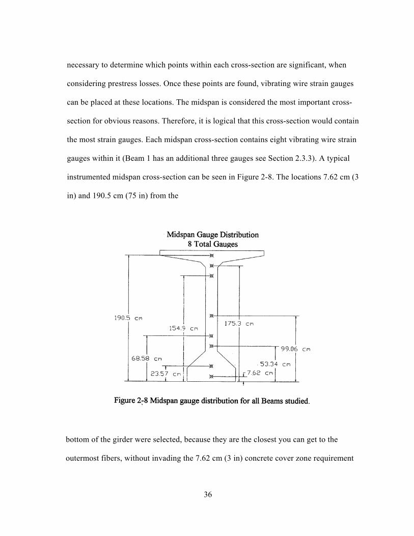
necessary to determine which points within each cross-section are significant, when
considering prestress losses. Once these points are found, vibrating wire strain gauges
can be placed at these locations. The midspan is considered the most important cross-
section for obvious reasons. Therefore, it is logical that this cross-section would contain
the most strain gauges. Each midspan cross-section contains eight vibrating wire strain
gauges within it (Beam 1 has an additional three gauges see Section 2.3.3). A typical
instrumented midspan cross-section can be seen in Figure 2-8. The locations 7.62 cm (3
in) and 190.5 cm (75 in) from the
bottom of the girder were selected, because they are the closest you can get to the
outermost fibers, without invading the 7.62 cm (3 in) concrete cover zone requirement
36

ACI Code 3 8R-89, Section 7.7.3.1.9 The location of 23.57 cm (9.28 in) represents the steel
centroi of all the prestressing strands within the cross-section. The choice of 99.06 cm (39
in) as made because this point is very close to the girder concrete centroid. The composite
section concrete centroid will occur at about 154.9 cm (61 in), after the deck is placed, so
this point was also chosen. The points 53.34 cm (21 in), 65.58 cm (27 in), and 175.3 cm (6
in) were picked to show the loss variation between the selected points of significance.
The uarter-span and 1.52 m (5 ft) from the support, each have 6 vibrating wire strain
gauge located throughout their respective cross-sections (Beam 1 has an additional three
gauges at the 1.52 m (5 ft) from the support see Section 2.3.3). Each of these cross-sectio s
contain the gauges placed at 7.62 cm (3 in), 175.3 cm (69 in), and 190.5 cm (75 in), whic
are similar to the midspan cross-section. The centroid of the steel in the bottom flange or the
straight tendons is 18.80 cm (7.4 in) for both cross-sections, and a gauge was paced at this
point also. An additional gauge was placed at the steel centroid of the drape strands for both
cross-sections. This location is 84.07 cm (33.1 in) at the quarter-span and 147.1 cm (57.9 in)
at the point located 1.52 m (5 ft) from the support. These two cross-sections can be seen in
Figures 2-9 for the quarter-span, and Figure 2-10 for the point 1.52 m (5 ft) from the end
support.
2.3.3 Gauge .Placement Along Strand
In addition to the cross-sectional variation of prestress, another area of interest was
how the stress would vary directly along the strands. For this an additional 6
37

29

vibrating wire strain gauges were placed in Beam 1. Three gauges were placed at 22.86
cm (9 in) from the bottom at the midspan, and the other three were placed at 17.78 cm (7
in) from the bottom at the point 1.52 m (5 ft) from the support. This gauges were directly
attached to the steel tendons at these locations, to secure them from shifting during
casting.
2.4 Composite Slab Instrumentation
2.4.1 Introduction
The girders of the Westbound Gandy Bridge are covered with a 20.32 cm (8 in)
continuous reinforced concrete deck slab over each three-span unit. This deck causes the
girder-deck combination to act as a single unit. Although this concrete deck is not
prestressed, it would be interesting to see how and if the prestress losses occurring in the
girders below it, would effect the slab's stress distribution. Figure 2-11 contains a top
view of the instrumented deck. Table 2-2 contains information about the depth, location,
and orientation of each gauge labeled in Figure 2-11.
39

31

2.4.2 Gauge Placement Along the Slab Longitudinal Axis
The choice of points along the slab in which gauges were placed was important,
especially, since the results obtained would have to work in conjunction with those from
the girders. The midspan of each girder would be a natural place, allowing a complete
stress distribution from the bottom portion of the girder to the top portion of the slab to be
determined directly. Other locations of interest are the points of maximum positive and
negative moment in the continuous deck.
2.4.3 Gauge Placement Across Depth of Slab
In the case of the girder, the gauges were placed parallel with the span of the
girder, in order, to obtain stresses in the axial direction. In the concrete deck, however; it is
important to obtain stress distributions in both the longitudinal and perpendicular
directions of the slab. This is necessary because applied loads create moments, which in
turn induce stresses in both directions within the deck.
The gauges were placed at approximately two depth locations within the slab.
These two depths are 0 and 10.16 cm (4 in), measured from the top of the girder. The
gauges placed at 0 represents the location where the interface between the girder and the
slab occurs. There should be a stress discontinuity occurring at this location. The point at
10.16 cm (4 in) was chosen because it is the mid-depth of the-20.32 cm (8 in) thick slab.
And in addition to this, it allows for a determination of the stress distribution between this
point and the 0 cm point.
41
2.5 Installation of Strain Gauges
2.5.1 Girder Strain Gauges
Effective installation of the vibrating wire strain gauges was imperative for this
research project to be successful. The strain gauges had to be installed securely, such that,
they would not shift during the casting of the beams. This was achieved by attaching the
gauges to two Number 3 steel rebars. These two rebars were separated by a distance
slightly smaller than the width of the gauge, and welded together by two pieces of steel.
The location of gauges were marked with chalk on the rebars, and then the gauges were
attached with steel tie wire. Finally, the gauge-rebar combination was tied securely to the
prestressed steel tendons to keep it in place.
Each of these strain gauges have a wire with a connector attached to its end. It was
very important to keep the connectors dry, so that they would not be damaged during
casting of the concrete. This was achieved by running the wires along the rebar and
placing the wires in several plastic bags above the top flange of the beam. After casting
and vibration of the concrete, the wires were removed from the bag and connected to the
multiplexers. Then, these multiplexers were connected to the data acquisition system
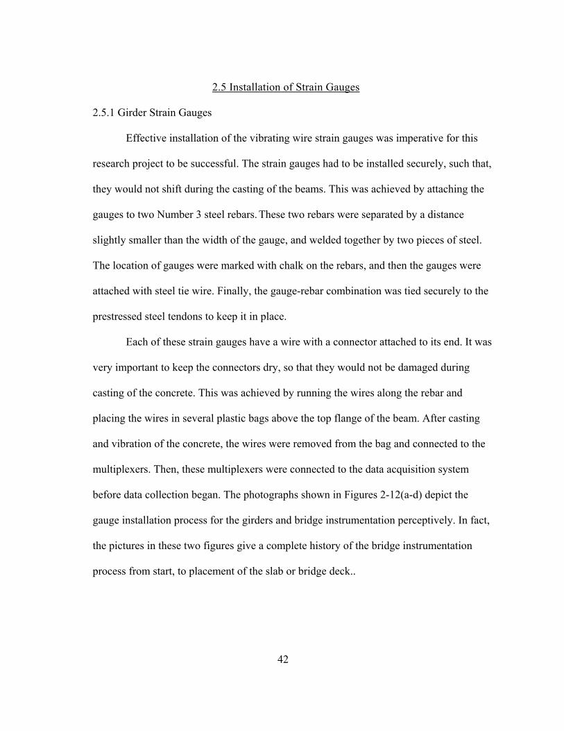
before data collection began. The photographs shown in Figures 2-12(a-d) depict the
gauge installation process for the girders and bridge instrumentation perceptively. In fact,
the pictures in these two figures give a complete history of the bridge instrumentation
process from start, to placement of the slab or bridge deck..
42

Figure 2-12a Preparation of strain gauges for placement in girders.
43

Figure 2-12b Shows placement of strain gauge within the girders.
44

Figure 2-12c Attachment of strain gauges along the steel strands.
45

Figure 2-12d The instrumented girders in the staging area awaiting shipment to the
bridge site.
46

2.5.2 Slab Strain Gauges
Instrumentation of the slab gauges promoted a different kind of problem, because
the slab forms and steel reinforcement were in place before the gauges could be installed.
The strain gauges could not be placed any time earlier, because they could be damaged
during the placement of the steel reinforcement for the slab. Hence, the strain gauges
were then attached to the steel rebar after the slab reinforcement was in place at the
specified locations using steel tie wire.
The connecting wire lengths were increased, by cutting and soldering longer
wires to them. Since the wires could not be placed earlier it was necessary for all the
wires to be feed below the steel reinforcement in the slab. This is because during casting
the workers walk directly on the reinforcement, and if the wires were caught between the
feet of the workers and the rebar, the wire could possibly be damaged.
To enable connection of the gauges to the multiplexers which were attached to
the web (see Section 2.6), it was necessary to cut holes in the bottom of the forms, and to
pass the wires through, to the multiplexers.
2.6 Equipment Attachment to Bridge
Once the girders were moved to the bridge -all equipment had to be permanently
secured to the bridge. The multiplexers were directly attached to the web of the girders.
A schematic of this can be seen in Figure 2-13. These multiplexers were attached with
47

5.72 cm (2-1/4 in) concrete bolts and a hammer drill. The strain gauge wires and
multiplexer wires connected to the data acquisition system required some sag, which
had to be accounted for. Using 1.27 cm (1/2 in) clips the wires were bolted to the web
of the adjacent girders.
The location of the data acquisition system was important because it had to be
easily accessed in case of a problem. The location selected was the pier between the
four instrumented beams. Along side of the datalogger is the 12-volt battery, both of
which are bolted using concrete bolts. This location allows for the datalogger to be
accessed by a ladder placed a the footer.
It was important to get the solar panel in an area where it would be directly
exposed to sunlight, in order to allow it to recharge the battery effectively. The relative
48

humidity and ambient temperature probe, and cellular phone antenna had to be in a
location where their readings or waves would not be inhibited. Hence, all of these three
pieces of equipment were attached to the outside of the pier. The wires from all these
three pieces of equipment are directly connected to the data acquisition system. Figure
214(a-c) shown pictures of the equipment attachments at the bridge site.
2.7 Shrinkage Cylinders
In a bid to separate the components of the time-dependent prestress loss, it is
important to get as much information about the concrete as possible. It was decided that
five 15.24 cm by 30.48 cm (6 by 12 in) cylinders would be casted for the purpose of
determining shrinkage strains in concrete. These cylinders were made from the same
concrete batch as used for the girders, and exposed to the same environmental
conditions as the girders.
Each of these shrinkage cylinders are instrumented with similar vibrating wire
strain gauges that were used in the girders and the deck. The gauge was placed in the
center of the cylinder mold, and held in place by three steel tie wires to allow
measurement of axial strain. These tie wires pass through small holes in the mold, and
are taped to the outside of the mold to hold it in place. A slit on the top of the mold was
left so the wire could be connected to the multiplexer.
49

Figure 2-14a Placement of girder on bridge pier and bridge deck with
50

Figure 2-14b Multiplexers attached to girder web with slack in the connecting wires.
51

Figure 2-14c Location of data acquisition system and battery (top) and solar panel, cellular phone antenna, and relative humidity probe (bottom).
52

The girders and cylinders were casted at the same time. The cylinders were
exposed to the same conditions as the girders from conception, to the bridge site. Once
at the bridge site, the cylinders were placed on an adjacent pier to that where the data
logger is located. The wires from the cylinders are attached to the side of the girders,
similarly, to those of the multiplexers and girder gauge wires. The photograph in
Figure 2-15a shows the preparation of a typical shrinkage cylinder mold before
casting. In Figure 215b. The shrinkage cylinders are depicted on top of the girder in the
stage area, and at their final location when moved to the bridge site.
Figure 2-15a A Preparation of shrinkage cylinder mold with strain gauge.
53

Figure 2-15b Shrinkage cylinders on top of the girder and at the bridge site.
54

2.8 Modulus of Elasticity
2.8.1 Introduction
The modulus of elasticity of any material directly relates the stress to the strain
according to Hooke's Law, which is a = E.s. The symbols a, E, and s, are the stress,
modulus of elasticity, and strain for a given material, respectively. For concrete, this
linear relationship holds true initially, but becomes nonlinear after a certain point.
2.8.2 ACI 318-89R Definition of E,
The American Concrete Institute Building Code Requirements for Reinforced
Concrete of 1989, Revised in 1992 (ACI 318-89R), defines the modulus of elasticity of
material as; the ratio of the normal stress to its strain for either tensile or compressive
stresses under the proportional limit of that material as described in Section 2.1 of the
Code. For concrete, the 89R Code states in Section 8.5 Commentary that the modulus of
elasticity of concrete, E, is the slope of the line drawn from 0 to 0.45fic on a stress strain
curve, where f,' is defined as the 28 day compressive strength of concrete. It also states
that measured E,- values may range from 80 to 120 percent of the calculated value.
The equation suggested by the ACI to determine E,, is based on w, and fc'. Where
w,, is -the specific weight of the concrete in lb/ft3 and f,-' is in psi. For w,, ranging from
90 to 155 lb/ft3 the equation for E, in Section 8.5 of the Code is as follows:
55

And this is the equation typically used in design.
2.8.3 Experimental Determination of E,
The actual modulus of concrete tends to deviate as a function of time from the
equation suggested by ACI. A more accurate modulus for concrete could give a better
representation of what the actual prestress losses are. , With this in mind, an additional
twenty test cylinders, 15.24 cm by 30.48 cm (6 by 12 in) were cast from the concrete
batch used, so that the modulus of concrete could be determined experimentally.
The experiments would be performed at the CEEFL ( the Civil and
Environmental Engineering Field Lab) at the University of Central Florida. The
equipment used was a compressive strength machine manufactured by SATEC
Systems, Inc., Grove City, Pennsylvania, and a strain measuring box borrowed from the
Florida Department of Transportation Structures Laboratory, Tallahassee, Florida. The
strain gauges used were attached to the outside of the cylinder being tested. From the
testing, the following measurements of the compressive strength and elastic modulus
were recorded. Table 2-3 contains the experimental results from this testing. Due to
some inconsistencies in the laboratory results, it was determined that perhaps a more
sophisticated experimentally setup could achieve more reliable results. This setup
would include an automatic data acquisition system that remove the human error aspect
of trying to obtain the readings manually. In this report, another method of calculating
E., is used in order to avoid including large experimental errors in
56

the values obtained. The elastic modulus is an essential component in this study and is
needed to be computed as a function of time.
2.8.4 CEB-FIP Model Code 1990 Method for Determining E,(t)
In the text "Concrete Structures: Stresses and Deformations," by Ghali and
Farve10, it suggests a few different methods for determining the time-dependent modulus
of elasticity of concrete. The method used here is that which was suggested by the CEB-
FIP Model Code 1990." This committee suggests the following equation for determining
the 28 day modulus of elasticity:
57

In Equation 2.2, f,. is the mean compressive strength at 28 days in MPa, and fcmo is equal to
10 MPa. The mean compressive strength, fcmis related to the characteristic strength, fck, as
follows:
In Equation 2.3, the quantity Of is equal to 8 MPa. The characteristic strength, f .k is
obtained performing compression tests on 15.0 by 30.0 cm (6 by 12 in) cylinders stored in
water at 20 ± 2 °C and tested 28 days after casting. So Equation 2.2 can now be rewritten as
follows:
The time-dependent modulus E,(t) is estimated by the following equation:
where
58

In Equation 2.6, the time t is measured in days, and s is a coefficient depending on the type
of cement used. For rapid hardening high strength cements, s is equal to 0.2, as it was
taken for this project.
2.8.5 Calculating E,(t) and Comparing to Design
In order for Equation 2.6 to be effective, it is necessary to have a reliable source of
f ck. The closest quantity available to fck is fc’ at 28 days. The Quality Control personnel at
the Hardaway Company in Tampa, Florida, measured compressive strength, at time of
transfer, 7, and 28 days after the concrete was casted. For each beam, two tests were
performed for each day mentioned. The only values needed here are those for f,.' at 28
days. Since Beams 1 and 4 were casted on the same day using the same concrete batch,
their compressive strengths were averaged to come up with one value. Similarly, the
procedure was done for the compressive strengths of Beams 2 and 3. The results obtained
can be seen in Table 2-4. It is interesting to note that the original design was done on the
assumption of fc' of 44.8 MPa (6500 psi), but the strength achieved in the field was are
much greater. With the quantities in Table 2-4, it is now possible to obtain values of Ec(t).
These values will be included in Table 2-5 and compared to those from the original design.
59

Now that all the parameters have been established the calculation of Ec(t) can proceed. The
calculated values Ec' for Beams 1 and 4, and Beams 2 and 3, versus the design calculated
values are shown in Table 2-5. As mentioned earlier, the results using another method, the
ACI Committee 209 method for determining Ec(t) can be found in Appendix A. The actual
design was based on the CEB-FIP Method, hence it was used over the ACI Committee
Method in this study.
These Ec values according to CEB-FIP were used in determining the prestress loss of the
members analyzed in this project. Additional days, which were between those values
reported in Table 2-5, were calculated and used in the loss calculations as well.
60


CHAPTER 3
CODE TREATMENT OF PRESTRESS LOSS
3.1 Introduction
There are several different methods for determining the prestress loss of a
member. The accepted methods are defined by various legal bodies. The American
Association of State Highway and Transportation Officials (AASHTO) is the legal
body that sets the standards for bridge design. For prestressed concrete, the Prestressed
Concrete Institute (PCI) suggests the methods of design, for both prestressed and
precast concrete. The standards for both prestressed and conventional concrete are
specified by the American Concrete Institute (ACI).
These bodies have different methods for determining the prestressed loss for
various types of members. Although, the ACI and PCI methods stem from the same
article and will be combined as one. In the sections that follow, a brief overview of how
these bodies determine prestress loss will be presented and discussed. At the end, a
spreadsheet program will be used to calculate the results for the methods presented.
53

The units specified for the equations in this chapter are based on the English system of
units. It is the results of these equations that are then converted to SI units through the
conversion factors of Section 1.5.
3.2 AASHTO-LRFD Method for Determining Prestress Loss
3.2.1 Introduction
The AASHTO-LRFD12 method defines the prestress loss for both pretensioning
and post-tensioning in Section 5.9.5. The prestress loss is broken into an instantaneous
portion and a time-dependent portion. The AASHTO-LRFD method offers two options for
determining the time-dependent prestress loss. The first is a lump sum based on the type of
member being examined, the 28 day compressive strength of that member, and the partial
prestressing ratio. The other option is a refined calculation of each of the components of
the time-dependent loss.
3.2.2 Total Prestress Loss
The AASHTO-LRFD in Section 5.9.5.1 defines the total prestress loss for
pretensioned members that are constructed and prestressed in a single stage as follows:
∆fpT = ∆fpES + ∆fpSR + ∆fpCR + ∆fpR (3.1)
and for post-tensioned members:
∆fpT = ∆fpF +∆ fpA + ∆fpES + ∆fpSR + ∆fpCR + ∆fpR (3.2)
54

3.2.3 Instantaneous Losses
In Section 5.9.5.2 of the AASHTO-LRFD, it discusses the methods for determining
the instantaneous losses. These losses are comprised of anchorage set, friction, and elastic
shortening.
3.2.3.1 Anchorage Set Loss
In Section 5.9.5.1 of the AASHTO-LRFD, it states that the anchorage set loss is the
larger of two possible slips. The first slip is what is measured while the anchorage is
restraining the stress in the prestressing steel, before and at transfer. The other slip, is the
amount suggested by the manufacturer of the anchor system. The commentary to this
section recommends possible values-of slip, depending on the type of equipment used, if
none are available.
55

3.2.3.2 Frictional Losses
In Section 5.9.5.2.2 of AASHTO-LRFD, for pretensioned members that have draped
strands the frictional losses should be considered at the hold-down devices. For post-
tensioned members, the frictional losses between the duct and the prestressing strands can
be determined as follows:
AfpF = fpj (1- e-(Kx+µα)`) (3.3) The
variables in Equations 3.3 are as follows:
fp; = stress in the prestressing steel at jacking in ksi
x = length of a prestressing tendon from the jacking end to any point under consideration
in ft.
K = wobble friction coefficient (ft-1)
µ= coefficient of friction (1/Rad)
α = sum of the absolute values of angular change of prestressing steel path from jacking
end
e = base of the Napieran logarithms
This section also contains a table of values that can be used for K and µ depending on the
type of tendon and sheathing used.
3.3.2.3 Elastic Shortening
In Section 5.9.5.2.3 of AASHTO-LRFD, the methods for determining the elastic
shortening for both pretensioned and post-tensioned members are presented. The elastic
56

shortening loss for pretensioned members is as
The variables in Equations 3.4 are defined as follows:
fcgp = sum of concrete stresses at the center of gravity of prestressing tendons due to
the prestressing force at transfer and the self-weight of the member at the sections of
maximum moment (ksi)
Ep = modulus of elasticity of prestressing steel (ksi)
Eci = modulus of elasticity of concrete at transfer (ksi)
It also suggests that for the usual design of pretensioned members, that fcgp be
calculated at an assumed stress of 0.65fpu for stress relieved strands and high strength
bars and 0.70fpu for low relaxation strands.
For post-tensioned members, the elastic shortening loss is computed differently
and is as follows:
The variables in Equations 3.5 are defined as follows:
N = number of identical prestressing tendons
fcgp = sum of concrete stresses at the center of gravity of prestressing tendons due to
the prestressing force after jacking and the self-weight of the member at the sections of
maximum moment (ksi)
57

It also states that the elastic shortening results in Equation 3.5 can be lower if stage
stressing and retensioning procedures are used.
3.2.4 Lump Sum Approximation for Time-Dependent Losses
In Section 5.9.5.3 of the AASHTO-LRFD Code, it suggests the use of an
approximate method for determining the total of all the time-dependent losses. This
method can be used for pretensioned members, if the compressive strength at transfer is
greater than or equal to 24.1 MPa (3.5 ksi). It may also be used for post-tensioned
members, if the members are non-segmental with spans up to 48.8 m (160 ft), and if the
stress transfer occurs between 10 and 30 days after casting. In addition to the above
criteria the following material conditions must also be true for both types of tensioning:
the member must be constructed from normal weight concrete and be either steam or
moist cured, and the prestressing strands or bars used within in the member must have
normal or relaxation properties. Average exposure conditions and temperatures must be
felt by the member during its lifetime.
This approximate method is a function of f.' and PPR. Table 3-1 gives a listing of
the applicable equations when using this procedure. The variable PPR is the partial
prestressing ratio and is defined in Section 5.5.4.2 of the AASHTO-LRFD Code as
follows:
67

The variables in Equation 3.6 are defined as follows:
AB = area of non-prestressed tension reinforcement (in 2)
Apg =area of prestressing steel (in 2)
Fy = specified yield strength of reinforcing bars (ksi)
Fpy = yield strength of prestressing steel (ksi)
Table 3-1 Equations used for lump sum prestress loss calculation according to AASHTO LRFD
Type of Beam Level For Wires or Strands with For Bars with fpu = 145 or Section f =235 250, or 270 ksi 160 ksi
Rectangular Upper Bound 29.0 + 4.0 PPR 19.0 + 6.0 PPR Beams, Solid Average 26.0 + 4.0 PPR
Slab Box Girder Upper Bound 21.0 + 4.0 PPR 15.0
Average 19.0 + 4.0 PPR I-Girder Average 19.0 + 6.0 PPR
PPRfc 0.6
0.60.6'15.00.10.33 +
−−
Single T Upper Bound Double T, Average
PPRfc 0.6
0.60.6'
15.00.10.39 +
−
−
Hollow Core and Voided
PPRfc 0.60.6
0.6'15.00.10.33 +
−−
Slab
The values obtained from equations of Table 3-1 can be reduced if low relaxation strands
are used. Box girders can be reduced by 27.6 MPa (4.0 ksi). Rectangular beams, solid
slabs, and I-girders can be reduced by 41.4 MPa (6.0 ksi). Single T's, double T's, hollow
core, and voided slabs can be reduced by 55.2 MPa (8.0 ksi).
59
PPRfc 0.60.6
0.6'15.00.10.33 +
−−

3.2.5 Detailed Estimates of the Time-Dependent Losses
In Section 5.9.5.4 of the AASHTO-LRFD Code, methods for determining the
individual components of the time-dependent prestress loss are discussed. Creep, and
shrinkage of concrete, and steel relaxation make up the total time-dependent prestress loss.
The methods in this section can be applied to non-segmental prestressed members that
have spans less than 76.2 m (250 ft), normal density concrete, and at time of prestress have
a compressive strength of 24.1 MPa (3.5 ksi).
3.2.5.1 Shrinkage
In Section 5.9.5.4.2 of the AASHTO-LRFD Code, the shrinkage prestress loss is
only a function of one variable for both pretensioned and post-tensioned members. The
average annual ambient relative humidity, H, in percent, is that variable. The shrinkage
loss is as follows:
∆fpSR = (17.0 - 0.150H) (3.7)
∆fpSR = (13.5 - 0.123H) (3.8)
Equation 3.7 applies for pretensioned members, and Equation 3.8 applies to posttensioned
members.
3.2.5.2 Creep
In Section 5.4.5.4.3 of the AASHTO-LRFD Code, the creep loss is considered the
same for both pretensioned and post-tensioned members. And is defined as follows:
60

∆fpCR = 12.0fcgp – 7.0fcdp ≥ 0 (3.9)
The variables in Equation 3.9 are defined as follows:
f g, = concrete stress at the center of gravity of prestressing steel at transfer (ksi)
∆fcdp = change in concrete stress at the center of gravity of prestressing steel due to
permanent loads, except the load acting at the time prestressing force is applied.
3.2.5.3 Steel Relaxation
In Section 5.9.5.4 of AASHTO-LRFD Code, the steel relaxation loss is broken
into two portions for pretensioned members. The first portion is the steel relaxation that
begins after the strands are stressed, and ends upon transfer of the stress from the steel
to the concrete. This steel relaxation loss calculated at transfers is as follows:
( )pj
py
pjpR f
fftf
−=∆ 55.0
0.100.24log
1 (3.10)
( )
pjpy
pjpR f
fftf
−=∆ 55.0
0.400.24log
1 (3.11)
Equation 3.10 applies for stress-relieved strands and Equation 3.11 applies for low-
relaxation strands. The variables in Equations 3.10 and 3.11 are as follows:
t = time estimated in days from stressing to transfer (Days)
fpj = initial stress in the tendon at the end of stressing just before transfer(ksi)
fpy = specified yield strength of prestressing steel (ksi)
61

The second portion of the steel relaxation loss that applies for pretensioned members, takes
place after the stress is transferred. The steel relaxation loss in post-tensioned members
occurs only at this stage. The equations for this is as follows:
∆fpR2 = 20.0 - 0.4∆fpFS - 0.2(∆fpSR + ∆fpCR) (3.12)
∆fPR2 =20.0 - 0.3∆fpF - 0.4∆fpES - 0.2(∆fpSR + ∆fpCR) (3.13)
Equation 3.12 is for pretensioned members with stress-relieved strands and Equation 3.13
for post-tensioned members with stress-relieved strands. All variables are defined as
before. If low relaxation prestressing steel is used the value of MpR2 can be taken as 30%
of those obtained using Equations 3.12 or 3.13.
3.3 ACI-PCI Method
3.3.1 Introduction
In Section 18.6 of the ACI 318R-89'3 Code, are given the types of loss that should
be accounted for in prestress concrete design. It also only gives equations for determining
frictional losses in post-tensioned tendons. In the Commentary to this section, it suggests
using the ACI-ASCE Committee 423 Report 14 for estimating the prestress losses. This
same report is the premise for the method described in Section 4.5 of the PCI Handbook."
Since the report is the basis for both the ACI and PCI procedures, they have been
combined here as one method. Applicable sections from both the ACI and PCI will be
presented in this section.
62

3.3.2 Sources of Loss from ACI Code
In Section 18.6.1 of the ACI Code, definitions of the types of losses that should be
estimated when the effective prestress is being determined are given. There are many
different types of losses and these lead to the eventual reduction of the jacking stress to
effective prestress. The sources of loss that most be allowed for are as follows:
anchorage seat loss, elastic shortening, creep, and shrinkage of concrete, relaxation of
tendon stress, and friction loss due to intentional or unintentional curvature of the tendons
in post-tensioning.
3.3.3 Typical Range of Total Loss According to PCI
The PCI handbook in Section 4.5.2, suggests typical ranges of total prestress loss
depending on the type of concrete being used. For normal weight concrete members the
total loss may lie between 173 to 345 MPa (25 to 50 ksi). For sand-lightweight concrete
members the total loss may be between 207 to 3791VIPa (30 to 55 ksi).
3.3.4 Frictional Loss According to ACI
In Section 18.6.2 of the ACI Code, the equations for calculating the friction loss in
post-tensioned members are presented. The PCI Handbook suggests that this loss can be
,ompensated for by overstressing, and presents no method for calculating this (see Section
3.3.5). The ACI equations are as follows:
( µα+= xKlxs ePP )
if(Klx+µα) ≥ 0.3 (3.14)
63

Ps = Px (1+Klx + µα) if (K1x +µα) < 0.3 (3.15)
The variables in Equation 3.15- and 3.16 are defined as follows:
Ps = prestressing force at jacking end
Px = prestressing tendon force at any point x
K = wobble friction coefficient
µ = curvature friction coefficient
α = total angular change of prestressing tendon profile in radians from tendon jacking end
to any point x
The Commentary to this section of the ACI Code contains suggested values for p and a,
based on the type of prestressing medium being used.
3.3.5 Equations for Determining Prestress Loss According to PCI
In Section 4.5.3 of the PCI Handbook, the equations for determining prestress
losses are presented. It is interesting to note that the PCI Handbook suggests that because
anchorage seat and frictional losses are mechanical losses, that they can be made up for
by overstressing. Because of this argument those two types of losses are not considered in
the total loss equation of Section 4.5.3 of the PCI Handbook. The equation for total loss
of prestress is as follows:
T.L.= ES + CR + SH + RE (3.16)
The variables in Equation 3.16 are defined as follows:
T.L. = total loss (psi)
64

ES = elastic shortening
CR = creep of concrete
SH = shrinkage of concrete
RE = relaxation of tendons
The equation for elastic shortening is very similar to that which is suggested by the
AASHTO-LRFD and is as follows:
(3.17)
The variables for Equation 3.17 are as follows:
Krg = 1.0 for pretensioned members
Es = Ep in AASHTO
Fcir = fcgp in AASHTO
g
g
g
i
g
icircir I
eMI
ePAPKf −
+= (3.18)
The variables in Equation 4.16 are defined as follows:
Kcir = 0.9 for pretensioned members
Pi = initial prestress force after anchorage seating loss
e = eccentricity of center of gravity of tendons with respect to the center of gravity of
concrete at the cross-section considered
Ag = area of gross concrete section at the cross-section considered
Ig = moment of inertia of gross concrete section at the cross-section considered
65

Mg = bending moment due to dead weight of prestressed member and any other permanent
dead loads in place at time of prestressing
The equation for creep is similar to that of the AASHTO-LRFD, except that it incorporates
more variables, and it is as follows:
)( cdscirc
scr ffE
EKCR −= (3.19)
The variables in Equation 3.19 are defined as follows:
Kcr = 2.0 for normal weight concrete or 1.6 for sand-lightweight concrete
fcds = stress in concrete at center of gravity of tendons due to all superimposed permanent
dead loads that are applied to the member after it has been prestressed
Ec = modulus of elasticity of concrete at 28 days
s
sdcds I
eMf = (3.20)
The variables in Equation 3.20 are defined as follows:
M.,= moment due to all superimposed permanent dead loads applied after prestressing
The equation for shrinkage is dependent on many variables and is as follows:
SH = (8.2 x 10⁻⁶)KshEs x (1-0.06 V/S)(100-R.H.) (3.21)
The variables in Equation 3.21 are defined as follows:
Ksh = 1.0 for pretensioned members
66

V/ S = volume to surface ratio
R.H. = percent relative humidity
The equation for steel relaxation uses values selected based on the type of tendon used, and
on the ratio of initial prestress after immediate losses, fpi, to the ultimate strength of the
tendon, fpu. The equation is as follows:
RE = [Kre - J(SH + CR + ES)]C (3.22)
The values K,., and J are functions of the type of tendon used and can be found in Table 3-
2.The values of C, which is a function of the ratio fpi/fpu, are found in Table 3-3.
67

Table 3-3 Values of CfPi/fpu Stress-relieved strand or Stress-relieved bar or low
wire relaxation strand or wire 0.80 1.28 0.79 1.22 0.78 1.16 0.77 1.11 0.76 1.45 1.05 0.75 1.36 1.00 0.74 1.27 0.95 0.73 1.27 0.90 0.72 1.18 0.85 0.71 1.09 0.80 0.70 1.00 0.75 0.69 0.94 0.70 0.68 0.89 0.66 0.67 0.83 0.61 0.66 0.78 0.57 0.65 0.73 0.53 0.64 0.68 0.49 0.63 0.63 0.45 0.62 0.58 0.41 0.61 0.53 0.37 0.60 0.49 0.33
68

3.4 Spreadsheet Prestress Loss Results
The equations from the AASHTO and ACI-PCI were incorporated into a
spreadsheet, and calculated for each girder section considered in this project. These
sections are the midspan and the 1.52 m (5 ft) from the end support of Beams 1 and 4, and
the midspan, and quarter-span of Beams 2 and 3. The results for all of these sections are
similar. These results will be presented here in this section for the beams being
investigated. The midspan had to be done for both sets of beams because the time at
transfer times, and the concrete compressive strengths were different. These results are
presented in Table 3-4 and Table 3-5 of this report.
Table 3-4 Spreadsheet results for the midspan of all beams studied.
Results for Midspan of Beams 1 and 4 in MPa
Code ES CR SH RE TL
ACI-PCI 116.9 204.6 30.7 53.8 406.1
AASHTO 123.3 228.9 39.6 25.6 417.5
Results for Midspan of Beams 2 and 3 in MPa
Code ES CR SH RE TL
ACI-PCI 126.4 207.2 30.7 52.9 417.1
AASHTO 133.2 228.9 39.6 22.4 424.3
69

Table 3-5 Spreadsheet results for quarter-span and 1.52 m from the end support of the beams studied.
Results for Quarter-span of Beams 2 and 3 in MPa
Code ES CR SH RE TL
ACI-PCI 123.4 202.2 30.7 53.6 410.3
AASHTO 129.4 222.3 39.6 23.4 414.9
Results for 1.52 m from End Support of Beams 1 and 4 in MPa
Code ES CR SH RE TL
ACI-PCI 116.9 204.6 30.7 54.0 406.2
AASHTO 123.3 228.9 39.6 26.6 417.5
The total loss values are higher for Beams 2 and 3, than Beams 1 and 4 at the midspans.
The results for the quarter-span of Beams 2 and 3, and the 1.52 m (5 ft) from the end
support of Beams 1 and 4, will be shown in Table 3-5. These results, for all points
examined, will be plotted and compared with those obtained experimentally.
70

Chapter 4
DATA ANALYSIS AND EXPERIMENTAL RESULTS
4.1 Introduction
The thousands and thousands of strain readings collected from the datalogger on
the Westbound Gandy Bridge, are used to determine the prestress losses within the
girders. However, it is not practical to use every reading for this task of determining the
losses. Portions of the readings have various fluctuations that are not consistent with
adjacent measurements. In order to have smooth data to work with, the raw data was
filtered to eliminate large fluctuations in the measured values.
The data file is first collected as a ANSI -DOS based file with each entry separated
by commas and each row representing the readings taken at a particular time. This file is
then brought into Microsoft Excel, and each data reading is placed in a separate cell. This
allows the data to be easily manipulated.
A typical example of the raw data collected and imported into Microsoft Excel is
shown in Table 4-1. This represents only a small portion of the file because the full
version is very large. The first column represents the datalogger number. The year, Julian
date, and hour of collection, which is represented in military time, are in columns 2, 3, 4,
71

and 5, respectively. The sixth column is the battery voltage, which needs to be greater
than 12 Volts, in order, for data to be stored and collected properly at time of
collection. The remaining columns are used to report the data in pairs of strain and
temperature. In which, the first column in the pair is the strain reading in microstrain
(106 - the actual strain) and the second column is the temperature reading in °F for
each gauge. This sequence continues until the last two columns of collected data. The
last two, represent the ambient temperature in °F and relative humidity in percent(not
shown in Table 4-1).
Figure 4-1 is a plot of the raw data collected from the gauge at the steel
centroid, of the section at the midspan of Beam 3. This plot contains the microstrain
and internal temperature versus time for December 31, 1995. Figure 4-2 shows the
ambient temperature and relative humidity measured for the same time interval shown
in Figure 41. The measurements used for these plots are raw and continuous for the
interval shown. Raw in the sense that the readings are as measured, and before any
filtering have been included. This is done to illustrate that high fluctuations do occur
due to extraneous vibrations, and are not considered useful data. One suggested reason
why these fluctuations occur, is because, sudden electric noise from adjacent
equipment could cause such a disturbance.
72

Table 4-1 Example of the raw collected Col 1 Col 2 Col 3 Col 4 Col 5 Col 6 Strain Temp Strain113 1995 355 12/21/95 1300 12 632 2445 9 67 334 2474 2113 1995 355 12/21/95 1400 12 631 2447 5 67 605 2465 2113 1995 355 12/21/95 1500 12 631 2447 5 68 424 2461 3113 1995 355 12/21/95 1600 12 631 2445 2 69 69 2455 4113 1995 355 12/21/95 1700 12 638 2439 2 71 137 2448113 1995 355 12/21/95 1800 12 625 2432 6 72 548 2440 1113 1995 355 12/21/95 1900 12 624 2425 8 73 662 2434 4113 1995 355 12/21/95 2000 12 624 2419 1 74 875 2427 8113 1995 355 12/21/95 2100 12 619 2411 5 76 158 2421113 1995 355 12/21/95 2200 12 625 2404 2 77 409 2416113 1995 355 12/21/95 2300 12 618 2397 5 78 668 2415 5113 1995 356 12/22/95 0 12 618 2397 1 78 49 2421 8113 1995 356 12/22/95 100 12 618 2402 7 77 297 2430 4113 1995 356 12/22/95 200 12 618 2410 1 75 767 2439 3113 1995 356 12/22/95 300 1 2 619 2418 9 74 029 2448 1113 1995 356 12/22/95 400 12 612 2428 1 72 262 2457113 1995 356 12/22/95 500 12 619 2456 4 70 577 2465 7113 1995 356 12/22/95 600 12 611 2445 4 69 081 2475 3113 1995 356 12/22/95 700 12 612 2451 3 67 113 2482 9113 1995 356 12/22/95 800 12 612 2455 1 65 548 2486 6

4.2 Determination of Prestress Loss from Measured Data
The strain and temperature measurements used for determining the prestress losses,
were taken from the most consistent data at the particular days of interest. The difference
between the strain readings are what is important, because, our concern is determining the
change in prestress throughout the member with time.
The measured strain reading is made up of many different components which induce
strain. In order to determine the change in strain and corresponding stress that belongs to
prestress loss, it is necessary to extract these other components. These components consist
of temperature effects and weight effects. The temperature effects are
74

created within the concrete and the steel of the vibrating wire in the strain gauge itself. The
weight effects are felt by the member immediately upon cutting of the steel strands from
the abutments. These effects must be removed to determine strain change due to prestress
loss.
However to start with, it is necessary to determine a datum or reference to relate the
change in the strain to, so that all changes refer back to the same point. Since we are
dealing with two types of prestress losses (instantaneous and time-dependent), it becomes
essential that there has to be two different reference points. The instantaneous loss, which
is considered all elastic shortening, has its reference point as the last reading before the
prestressing strands were cut. The last point used in determining the elastic shortening is
the first reading taken after all the strands have been cut (3 hours after the first strand was
cut). This point is also used as the new reference or datum for determination of the time
dependent prestress losses.
The change in concrete strain due to prestress, єprestress, is determined by the
following equation:
∆є Prestress – ∆єTotal - єTemp. - єWeight Effects (4-1)
Equation 4-1 extracts the prestress strain difference from the overall change in strain. Each
of the components of this equation will be explained in detail in the following paragraphs.
75

The change in total strain, D£Totai, is the difference between the strain readings,
after temperature corrections of the steel in the vibrating wire strain gauges have been
accounted for. This temperature correction is represented in the following equation:
∆є Total =(є t – є 0) + (T t – T t-1) x 6.78 (4-2) In
Equation 4-2, є and T represent the strain reading in microstrain and the internal temperature,
respectively. The subscripts, t and 0, represent the readings at any time t and at a reference
point 0. The subscript t-1 is the temperature reading used for the previous determination of
the ∆єPrestress. The 6.78 multiplied with the internal temperature change is the coefficient of
expansion of the steel used for the vibrating wire in the strain gauge. This number was
recommended by Geokon Inc. and has the units of micro-strain/°F.
The strain created from the change of internal temperature within the concrete is
ETomp. This strain can have large effects on the overall strain, in a concrete member, and
must be removed to extract ∆єPrestress. The equation for єTemp is as follows:
є Temp = 5.5 x (Tt – Tt-1) (4-3) In
Equation 4-3, the 5.5 multiplied with the internal temperature change is the coefficient of
expansion of concrete and has the units of micro-strain/°F. All the other terms in Equation 4-
3 are defined as before.
Another portion of the total strain that must be removed is the strain that is created
from the weight effects, £weigt Eff tr. The weight effects need to be considered
immediately after the strands are cut. At this time the members camber upward, and the force
due to the self weight is pulling against it. The standard equation for determining the stress
76

created by the weight effects can be converted to strain through its relationship with the
Young's Modulus. The stress equations due to weight effect is as follows:
Equation 4-4 and Equation 4-5 represent the stress in the top and bottom portions of the
member, with respect to the neutral axis, respectively. These portions are separated by the
concrete centroid, cConc with units of inches. Mo is in k-ft and is the moment created by
the self weight of the member. IConc is the moment of inertia of the concrete section in in4.
Both Equation 4.4 and Equation 4.5 will yield stresses in ksi.
The initial prestress force and stress is based upon the force applied to the area of
steel present. In determining the prestress losses of a member, it is usually customary to
calculate them is terms of equivalent steel throughout the cross-section. This then makes
it necessary to convert the strain changes in the concrete to equivalent stress changes in
the steel. It is assumed that changes in the concrete strains and the prestressing steel, are
equivalent because of the strong bond between them. The change in steel stress is
obtained by multiplying the change of strain extracted from the gauges in the concrete by
the modulus of elasticity of the prestressing steel. The equation for this is as follows:
∆fprestress = Es - ∆є Prestress (4-6)
For the Westbound Gandy bridge the modulus of the prestressing steel, Es, is 28,000 ksi
77

4.3 Ambient Temperature and Relative Humidity
Ambient temperature and relative humidity are considered important factors when
examining the time-dependent behavior of prestressed concrete. This is especially true when
studying shrinkage of concrete, as mentioned in Section 1.3.3.2 of this report. Shrinkage in
turn affects the concrete creep and steel relaxation also.
In the case of the Westbound Gandy Bridge project all beams were investigated not
cast on the same day. Beams 1 and 4, were cast five days before Beams 2 and 3, under
different environmental conditions. Figures 4-3 and 4-4 contain the ambient temperature and
relative humidity plots for Beams 1 and 4, and Beams 2 and 3, respectively. The points on
these plots cover the same time intervals, selected for determination of the change in prestress
force. An average of the conditions on each day was computed and plotted.
4.4 Immediate Prestress Loss
4.4.1 Introduction
In the case of the Modified AASHTO Type VI pretensioned prestress girders used on
the Westbound Gandy bridge, it is assumed that all of the immediate prestress loss is elastic
shortening. Anchorage slip and frictional losses were considered negligible in comparison to
elastic shortening. The steel relaxation before the strands were cut was also considered
negligible.
78


The portion of the prestress loss associated with elastic shortening is said to occur
simultaneously, with the application of the prestress from the steel strands to the concrete.
The cutting of the strands take place approximately over a 3-hour period. Since this loss is
considered a one time loss, it has an absolute start and end point. Therefore, the beginning
reference point was selected just before the strands were cut. The end reference point used
in the analysis was chosen at the time the cutting was finished. With this simple
assumption, elastic shortening loss can be determined for all locations where data was
available. Initial data for Beam 2 is unavailable and is not considered in this analysis.
4.4.2 At Midspan
The elastic shortening results obtained for midspans of Beams l, 4, and 3, can be
seen in Figures 4-5, 4-6, and 4-7, respectively. The differences between Beams 1 and 4, and
Beam 3, is the age of the concrete when the prestressing strands were cut, and the ambient
conditions (temperature and relative humidity). At the time the strands were cut, the age of
concrete for Beams 1 and 4 were five days old, while Beam 3 was three days old. Also
included on the plots are the elastic shortening results calculated by the ACIPCI and
AASHTO equations of Chapter 3. In examining these plots there are clear trends, ranging
from small changes in the top flange, to gradually larger changes toward the bottom flange.
The elastic shortening results are larger for Beam 3, than those of Beams 1 and 4. A
possible reason for this may be that the gauges were shifted during casting of the beams,
causing their position not to be parallel with the span.
80

81

Figure 4-8 contains an average of the elastic shortening of the three midspans
for five points of interest. At the steel centroid, 23.6 cm, where the average elastic
shortening loss is -221.6 MPa. Results for elastic shortening at the concrete centroid,
which is at approximately 99.1 cm, is -123.1 MPa. At the future composite centroid,
154.9 cm, the elastic shortening loss was -56.6 MPa. At 175.3 cm which is
approaching the top flange, the loss is -36.6 MPa, and at 190.5 cm which is 7.6 cm
from the top flange, the elastic shortening loss is -21.0 MPa. The value at the concrete
centroid is quite close to that of the Code results. At the steel centroid, however, the
elastic shortening loss is much larger.
82

4.4.3 At Quarter-span and 1.52 m from Support
The results obtained for the quarter span of Beam 3, and at the point 1.52 m
from the end support of Beams 1 and 4, can be seen in Figures 4-9, 4-10, 4-11,
respectively. These three Figures follow the same trend as the midspan loss, that is the
change is relatively small near the top flange, and gradually increases as you move
down the crosssection. This trend is consistent with the expectation, that greater values
of loss will occur closer to the area where the prestressing strands exist. The magnitude
of the loss seems to be smaller, at the quarter span and 1.52 m, when compared to the
midspans.
For the quarter-span, four points of interest are 190.5 cm (top flange), 175.3 cm
(near the future composite centroid), 84.1 cm (near the concrete centroid), and 18.8 cm
83

84

(straight strand steel centroid). The results for elastic shortening at 190.5 cm, 175.3 cm,
84.1 cm, and 18.8 cm are -0.92, -8.7, -151.4, and -241.4 MPa, respectively.
For the 1.52 m mark, the four points chosen for averaging of Beams 1 and 4 data
are 190.5 cm., 175.3 cm, 147.1 cm (near the future composite centroid), and 18.8 cm. The
results for the average of Beams 1 and 4 at the 1.52 m mark are shown in Figure 4-12. In
that Figure, for 190.5 cm., 175.3 cm, 147.1 cm, and 18.8 cm, the elastic shortening loss is
-24.7, -38.6, -65.0, and -154.1 MPa, respectively.
85

4.4.4 Variation Along the Length of the Beam
The elastic shortening loss has been represented at points within the cross-section
without any variation along the length of the beam. The average values at the points of
interest will now be plotted with consideration to length as well as depth. Since at the time
of this study (150 days), all beams are under similar loading, it is reasonable to
superimpose data from the midspan of 21.95 m, quarter-span of 10.97 m, and the 1.52 m
from the end support, in order to determine the lengthwise variation of the losses.
Figure 4-13 shows the elastic shortening variation with length for the above
mentioned points. It is assumed that at this time, the loading is symmetric so the results
from one side can be flipped to the other. The steel centroid loss is larger at the quarterspan
than at the midspan, but much smaller at the 1.52 m mark. The concrete centroid
86

loss is greater at the quarter-span, when compared with that of the midspan. The loss at the
level of the future composite centroid seems constant at the 1.52 m and the midspan points
(there is no gauge at this location at the quarter-span, although the line is extended through
that point). For the 190.5 and 175.3 cm points, the loss is very similar at the 1.52 m and
midspans but is less at the quarter-span for these points.
4.5 Time-Dependent Prestress Loss
4.5.1 Introduction
The time-dependent prestress loss is made up of creep, shrinkage of concrete, and
steel relaxation. This section does not break the time-dependent prestress loss into its
87

individual components, but it examines this loss without including the effect of elastic
shortening.
It is assumed that the time-dependent portion of the prestress loss begins to occur
directly after the immediate losses or when the strands are all cut. This point serves as a
reference point to which all time dependent losses will be referred back to. Hence, the
loss calculated at any time, t, will encompass all of the time-dependent loss up to that
moment in time.
4.5.2 At Midspan
The results obtained for the time-dependent loss at the midspans of Beams 1, 4,
and 3, can be seen in Figures 4-14, 4-15, and 4-16, respectively. These plots show data
from all gauge locations that occur within the girder cross-sections. There seems to be
little or no variation between the slopes of the time-dependent portion of the curves for all
the gauges. Also shown are the calculated time-dependent prestress losses from ACI-PCI
and AASHTO equations of Chapter 3.
Figure 4-17 contains an average time-dependent loss over the 150 day period, for
five points of interest that occur in the midspan. These points are 190.5, 175.3, 154.9,
99.1, and 23.6 cm, and the time-dependent losses are -77.5, -87.1, -96.0, -134.3, and -
193.6 MPa respectively. .
88


4.5.3 Quarter-span and 1.52 m from Support
The results obtained for the quarter span of Beam 3, and the 1.52 m points in
Beams 1 and 4, are Figures 4-18, 4-19, and 4-20, respectively. They follow the pattern
whereby they are progressively larger as you move from the top portion of the beam to the
bottom. There seems to be little variation between the time-dependent loss at quarterspan
and that at 1.52 m.
For the quarter point of Beam 3, the time-dependent loss over the 150 day period
for four points of interest are shown in Figure 4-18. For the points 190.5, 175.3, 84.1, and
18.8 cm the time-dependent losses is -80.0. -102.3, -153.3, and -195.9 MPa, respectively.
These values are just slightly larger than at 190.5 cm and 175.3 cm of the midspan, and
slightly smaller than at the steel centroid (23.6 cm) of the midspan.
The average time-dependent loss for Beams 1 and 4 for the selected points at 1.52
m is shown in Figure 4-21. For 190.5, 175.3, 147.1, and 18.8 cm, the losses are -85.0, -
93.7,-104.6, and -164.75 MPa, respectively. The top point losses of the 1.52 m mark are
larger than those at quarter-span and midspan, and the bottom point losses are less than at
the quarter-span.
4.5.4 Variation Along the Span
The average time-dependent prestress loss variation along the span is plotted in
Figure 4-22. The time-dependent prestress loss is very similar for the 1.52 m, quarterspan,
and midspan, at the 190.5 cm and the composite centroid levels. At 175.3 cm the
91


loss is larger for the quarter-span than the midspan and 1.52 m points. The concrete
centroid is larger for the quarter-span than the midspan. The steel centroid level loss is
larger for the midspan and quarter-span when compared with the 1.52 m points.
4.6 Lump Sum Prestress Loss
4.6.1 Introduction
The lump sum prestress loss is made up of both the immediate and time-dependent
prestress loss. This is considered the total prestress loss at any time t. And for this section t
is equal to 150 days.
94

4.6.2 At Midspan
The results obtained for the lump sum loss at the midspans of Beams 1, 4, and 3,
can be seen in Figures 4-23, 4-24, and 4-25, respectively. These plots show all gauge
locations that occur within the section. There seems to be little or no variation between the
slopes of the time-dependent portion of the curves for all the gauges. Also shown are the
calculated time-dependent prestress losses from ACI-PCI and AASHTO equations of
Chapter 3.
Figure 4-26 contains an average lump sum loss over the 150 day period for five
points of interest that occur in the midspan. For the points 190.5, 175.3, 154.9, 99.1,
and 23.6 cm, the lump sum loss is -98.6, -123.7, -152.6, -257.4, and -415.2 MPa
respectively. The loss at the steel centroid level has already surpassed the ACI-PCI lump
sum estimate and is very close to the AASHTO estimate.
4.6.3 At Quarter-span and 1.52 m from Support
The results obtained for the quarter span of Beam 3, and the 1.52 m points in
Beams 1 and 4 are in Figures 4-27, 4-28, and 4-29, respectively. They follow the pattern
whereby they progressively get larger as you move from the top portion of the beam to the
bottom. There seems to be little variation between the lump sum loss at quarter-span and
that at 1.52 m.
95


For the quarter point of Beam 3, the lump sum loss over 150 day period for the four
points of interest are shown in Figure 4-27. For the points 190.5, 175.3, 84.1, and 18.8 cm,
the lump sum loss is -80.9. -111.0, -304.7, and -438.3 MPa respectively.
The average time-dependent loss for Beams 1 and 4, for the selected points at 1.52
m is shown in Figure 4-30. For 190.5, 175.3, 147.1, and 18.8 cm, the losses are -109.8, -
132.3,-169.6, and -318.8 MPa, respectively.
4.6.4 Variation Along the Span
The average lump sum prestress loss variation along the span is plotted in Figure 4-
31. The lump sum loss is very similar for the 1.52 m, quarter-span, and midspan at 190.5,
175.3 cm, and the composite centroid levels. At the concrete centroid the loss is larger for
the quarter-span then the midspan. However, at the steel centroid level, the loss is larger
for the midspan and quarter-span compared with the 1.52 m points.
The results observed here will be used to determine the effects of these prestress
losses on prestressed concrete bridge design in the next chapter.
100

Figure 4-31 Lump sum loss variation along the
101

CHAPTER 5
EFFECTS OF PRESTRESS LOSS ON BRIDGE DESIGN
5.1 Introduction
In the previous chapter, the methods used to obtain the actual prestress losses were
presented and the results shown. In this chapter, the losses are further examined to better
understand their effects on bridge girder design. This is important because in design the
prestress loss is generally assumed to be constant across the cross-section at any particular
location being examined. Since this is not the case in reality, it is necessary to see the
effect this has on other areas of design, such as, in other areas such as in the levels of
concrete and tendon stresses, as well as, camber and deflection.
This chapter mainly examines three beams, using data at different locations along
the span unless otherwise stated. The locations selected are the midspan of Beam 1, the
quarter-span of Beam 3, and the 1.52m (5 ft.) from the end support of Beam 4. The results
of the other cross-sections are similar.
To begin with, the cross-sectional prestress loss distribution on specific days are
superimposed on the same plot for either 3 or 4 different days, to provide continuous time-
dependent variation of the losses. Then the various ratios and percentage losses are
102

shown to further illustrate the effects of the losses throughout the cross-sections. Also,
the stresses in both the prestressing tendons and concrete are computed and compared to
their allowable values as stated in the ACI Code. Plots of relative humidity and ambient
temperature versus loss for the midspan of the all beams studied are presented, and a
regression analysis is performed to establish the level of dependency of the losses on
these parameters, all things being equal. Finally, the effects of the prestress loss on the
camber and deflection of the girders are studied.
5.2 Cross-sectional Prestress Loss Variation
Prestress losses are generally assumed to be uniform across the section of a
member being examined during design. In reality this is not the case. The
experimentally determined prestress loss varies considerable from the bottom to the top
of a member. This variation appeared to be essentially linear within each specified
cross-section. Therefore, having a better understanding of the prestress loss variation
throughout a cross-section, allows for a more accurate determination of concrete and
tendon stresses after transfer, and under service conditions.
The cross-sectional prestress loss results are plotted for the following days: l, 3,
7, 14, 28, 50, 60, 90, 120, and 150 days. These days are consistent with those chosen for
the girder design also. There are four plots for each cross-section examined, which will
be presented in one figure per cross-section. The plots are in the following sequence: 1.
103

3, and 7 days, 7, 14, and 28 days, 28, 50, and 60 days, 60, 90, 120, and 150 days. The
calculated ACI-PCI and AASHTO prestress, loss results are assumed uniform and are
superimposed on each plot as well. Note that the days are measured from when the transfer
of stress from the prestressing strands to the concrete occurs.
5.2.1 Midspan of Beam 1
The cross-sectional prestress loss versus depth for the midspan of Beam 1 is plotted
in Figure 5-1(a-d). In Figure 5-la, there is only a slight change of the crosssectional loss
between 1 and 3 days, but the gap then widens upon 7 days. At 7 days the gauge at 7.6 cm.
(3 in.) approaches the ACI-PCI calculated loss. The loss at 190.5 cm. (75 in.) is actually
positive signifying the location was becoming less tensile.
In Figure 5-lb, a larger gap appears between 7 and 14 days, but the is little variation
between 14 and 28 days. After 14 days, the gauge at 7.6 cm. (3 in.) is beyond the ACI-PCI
calculated loss, and the loss at the steel centroid, which is located at 23.6 cm. (9.3 in.), is
approaching the ACI-PCI loss. The loss at 190.5 cm. (75 in.) is still positive at 28 days.
In Figure 5-lc, a larger variation is shown between 28 and 50 days with little or no
change at all between 50 and 60 days. The value of the loss at the steel centroid goes beyond
the ACI-PCI calculated loss by 50 days. The entire loss is now all showing negative values
as of 50 days.
104


In Figure 5-1 d, clearly indicates that the loss increases at a decreasing rate, as time elapses
This can be seen by the gradual decrement in the gaps between the days shown. The
prestress loss for 150 days at location 53.3 cm. (21 in.) is now approaching the ACIPCI
calculated loss, and the loss at 7.6 cm (3 in.) is approaching the AASHTO calculated loss.
5.2.2 Quarter-span of Beam 3
The cross-sectional prestress loss versus depth for the quarter-span of Beam 3 is
shown in Figure 5-2(a-d). In Figure 5-2a, the change between 1 and 3 days is larger than the
change between 3 and 7 days for this cross-section. At 7 days the gauge at the
straight prestressing steel centroid, 18.8 cm. (7.4 in.), is equal to the ACI-PCI calculated
loss. Initially, at 190.5 cm. (75 in.) and 175.3 cm. (69 in.) the positive loss shows that these
locations are becoming less tensile. After 7 days , however, only the 190.5 cm. (75 in )
remains in the positive loss zone.
In Figure 5-2b, a smaller gap is shown between 7 and 14 days than between 14 and
28 days. The loss at 34.0 cm (13.4 in.) is gradually approaching that of the ACI-PCI 28
days. The loss at 190.5 cm. becomes negative after 14 days.
In Figure 5-2c, it is interesting to note that the difference between the loss at 50 and
60 days is more pronounced than at the midspan of Beam 1. At 50 days, the value of the
loss at 34.0 cm. is equal to the ACI-PCI calculated loss. And at 18.8 cm., the loss is
approaching the AASHTO calculated loss.
107


Figure 5-2d is similar to Figure 5-ld in that it shows a decreasing rate of the loss
increment between the days. However, the rate at which the decrement occurs is more
gradual than at the midspan. The prestress loss by 150 days at 18.8 cm. has reached the
calculated AASHTO loss value. These plots are very similar to those of the midspan of
Beam 1, but show a more linear variation of the loss over the depth of the beam.
5.2.3 From the End Support (1.52 m) Beam 4
The cross-sectional prestress loss versus depth at 1.52 m (5 ft.) from the end
support for Beam 4 is shown in Figure 5-3(a-d). In the first plot, Figure 5-3a, the loss
appears to be occurring at higher rate in the lower portion of the cross-section than in the
upper. There is no positive loss at this cross-section, suggesting little tensile stresses this
close to the support..
Figure 5-3b shows a trend towards a more uniform rate of loss between the top
and bottom with little change between 14 and 28 days. However, the change between 7
and 14 days is much greater.
Figure 5-3c is consistent with that of Figure 5.3b except there is a larger change
between 28 and 50 days while remaining relatively unchanged between 50 and 60 days.
In Figure 5-3d, the loss starts showing a more consistent rate of decrement, and the
separation per month going to 150 days is approximately equal. It is interesting to
110


note that the losses for this cross-section are much less than those computed by either
ACI-PCI and AASHTO methods.
5.2.4 Discussion
The behavior of the cross-sectional prestress loss variation for the days mentioned
is very similar for both midspan of Beam 1 and the quarter-span of Beam 3. Both have
locations where the stress is becoming less tensile towards the top. At 7.6 cm from the
bottom, they both reach the ACI-PCI computed loss in approximately 7 days and the
AASHTO computed loss in about 150 days. The losses at 1.52 m from the end support has
no location that is becoming less tensile, and does not even come close to reaching the
values of loss calculated by the ACI-PCI and AASHTO methods. The magnitude of the
loss is generally greater at the midspan and the quarter-span than, at 1.52 m from the end
support.
5.3 Percentage Comparisons of the Prestress Loss
5.3.1 Introduction
So far the prestress loss has been represented by the value actually occurring at a
specific location. An example of this is the lump sum prestress loss at the steel centroid of
Beam 1 for 150 days is 430.6 MPa. In this section, the prestress loss is taken as
113

defined ratios to have a better understanding of what all these numbers actually mean, with
respect to prestressed concrete girder design.
5.3.2 Initial Prestress to Jacking Stress Ratio
The initial prestress, fi, is defined as the prestress after all immediate losses have
occurred. The immediate losses, in this report, are assumed to be all elastic shortening. The
initial prestress can be computed as follows:
fi - fpi - ∆fES (5-1)
In Equation 5-1, fpj is the jacking stress and ∆fES is the loss of prestress due to elastic
shortening. The jacking stress, fpj, was consider uniform throughout the cross-section and
was determined as follows:
ps
jpj A
Pf = (5-2)
In Equation 5-2, Pj represents the jacking force on one strand and A, is the crosssectional
area of one prestressing strand. For the case of the Westbound Gandy Bridge, Pj is equal to
150.4 kN (33.8 kips) and 4 is equal to 1.08 cm2 (0.167 in). Applying these quantities in
Equation 5-2 results for 1395 MPa (202.4 ksi), for the jacking stress.
Now that these parameters have been defined the initial prestress to jacking stress
ratio is defined as follows:
pj
ESpj
pj
pi
fff
ff ∆−
= (5-3)
114
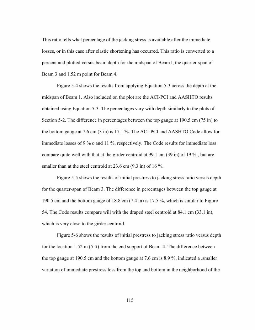
This ratio tells what percentage of the jacking stress is available after the immediate
losses, or in this case after elastic shortening has occurred. This ratio is converted to a
percent and plotted versus beam depth for the midspan of Beam l, the quarter-span of
Beam 3 and 1.52 m point for Beam 4.
Figure 5-4 shows the results from applying Equation 5-3 across the depth at the
midspan of Beam 1. Also included on the plot are the ACI-PCI and AASHTO results
obtained using Equation 5-3. The percentages vary with depth similarly to the plots of
Section 5-2. The difference in percentages between the top gauge at 190.5 cm (75 in) to
the bottom gauge at 7.6 cm (3 in) is 17.1 %. The ACI-PCI and AASHTO Code allow for
immediate losses of 9 % o and 11 %, respectively. The Code results for immediate loss
compare quite well with that at the girder centroid at 99.1 cm (39 in) of 19 % , but are
smaller than at the steel centroid at 23.6 cm (9.3 in) of 16 %.
Figure 5-5 shows the results of initial prestress to jacking stress ratio versus depth
for the quarter-span of Beam 3. The difference in percentages between the top gauge at
190.5 cm and the bottom gauge of 18.8 cm (7.4 in) is 17.5 %, which is similar to Figure
54. The Code results compare will with the draped steel centroid at 84.1 cm (33.1 in),
which is very close to the girder centroid.
Figure 5-6 shows the results of initial prestress to jacking stress ratio versus depth
for the location 1.52 m (5 ft) from the end support of Beam .4. The difference between
the top gauge at 190.5 cm and the bottom gauge at 7.6 cm is 8.9 %, indicated a .smaller
variation of immediate prestress loss from the top and bottom in the neighborhood of the
115


girder support. The Code results correspond quite well with those of the straight steel
centroid 18.8 cm.
The girder results compare well with those of the Codes at both the midspan of
Beam 1 and the quarter-span of Beam 3. However, the straight steel centroid results at
the 1.52 m from the end support compare favorably to the Code values. Although they
seem to correspond well at the girder centroid, the straight steel centroid indicates more
immediate loss than the Codes suggest.
117

5.3.3 The Effectiveness Ratio, R
The effectiveness ratio, R, is a parameter defined by Nilson16 which relates the effective
prestress force, Pe, at any time t to the initial prestress, Pi. The effectiveness ratio is as
follows:
i
e
PPR = (5.4)
This ratio can easily be converted into stress by dividing Po and P; by the area of
prestressing steel A., that corresponds to Pe and P;. Then the effectiveness ratio takes this
form:
pi
pe
ff
R = (5-5)
In Equation 5-5, fpe can be taken at any time t to determine the effectiveness ratio at that
time. The effective prestress, fpe is computed as follows:
fpe = fpi - ∆fTD (5-6)
In Equation 5-6, Af,D represents the time-dependent loss occurring up to the time
examined. The effectiveness ratio, describes how much prestress in terms of percent of fpi
is still available for the use in the girder. Nilson also suggests (1-R) as another interesting
quantity to investigate and is represented here in terms of stress as follows:
pi
TD
pi
pepi
ff
fff
R ∆=−
=−1 (5-7)
118

Equation 5-7 relates the time-dependent loss at any time t to the initial prestress. The plots
in this section are set with t = 150 days, that means., AfTD is the time-dependent loss
occurring up to this time.
Figure 5-7 contains the plots of R and 1-R versus depth for the midspan of Beam
1. The percent difference between the values of R at 190.5 cm (75 in) and 7.6 cm (3 in) is
11.5 %. The values from the ACI-PCI and AASHTO procedures are being approached at
the 7.6 cm mark and the steel centroid 23.6 cm (9.3 in), but the value at the girder
centroid is some degree higher. The higher the value of R, the more the stress that is still
available at the location. From the 1-R plot only 4.8 % of the initial prestress for the
location at 190.5 cm has been lossed as opposed to 16.3 % at 7.6 cm. The ACI-PCI and
the AASHTO Codes provide for 20 % and 25 % time-dependent losses, respectively.
Figure 5-8 contains the plots of R and 1-R versus depth for the quarter-span of
Beam 3. The percent difference between the values of R at 190.5 cm and 18.8 cm is 10.6
%. The value of R at 18.8 cm is somewhat larger than the computed Code values. Forthe
1-R plot, the 190.5 cm location has a time-dependent prestress loss of 5.1 % which differs
greatly from the location of 18.8 cm of 15.7 %. These losses are much smaller than the
Code suggested values up to this time
Figure 5-9 represents the plots of R and 1-R for the location 1.52 m from the end
support. The percent difference between the values of R at 190.5 cm and 7.6 cm is 6.6 %,
which is again getting smaller, as was the case for the immediate losses. All values of R
throughout this cross-section are far from those of the ACI-PCI and AASHTO computed
119


values. For the 1-R plot, 5.7 % of the time-dependent prestress loss has been lost at 190.5
cm compared to 12.3 % at 7.6 cm. If the Code values are to be used as a datum, this
suggests that much more time-dependent loss can be expected in the future.
The percent differences for R between the top and bottom, at the midspan of
Beam 1 and the quarter-span of Beam 3, are 11.5 % and 10.6 % which are very similar.
The location 1.52 m from the end support of Beam 4 shows much less at 6.6 %. This
suggests that the support location contains a more uniform loss throughout the cross-
section compared to the others. The 1-R values for 190.5 cm were 4.8 %, 5.1 %, and 5.7
% for the midspan, quarter-span and the location 1.52 m from the end support. This trend
shows that the time-dependent loss increase slightly in the top portion of the member, the
further away you go from the midspan. The steel centroid at the midspan and the straight
strand centroid at the quarter-span have almost equal losses at 15.8 % and 15.7 % o
respectively. The loss at the level of the straight strand centroid at the location 1.52 m
from the end support drops off to only 12.3 %. This suggests that the time-dependent
losses are felt greater toward the midspan, than at the supports, and areas with higher
concentration of the prestressing steel.
5.3.4 Lump Sum Loss to Jacking Stress Ratio
The lump sum loss to jacking stress ratio tells what percentage of the applied
jacking stress is lost. This is important because knowledge of this ratio can be allowed for
123

in design, so that more realistic service stresses can be obtained. The lump sum loss
reported includes immediate losses and the time-dependent losses occurring up to 150
days.
Figure 5-10 shows the lump sum loss to jacking stress ratio versus depth for the midspan
of Beam 1. There are significant differences from the top of the cross-section to its
bottom. At 190.5 cm, there has only been a 4.9 % loss, compared to 31.2 % loss at 7.6
cm. At both 23.6 and 7.6 cm, the percent loss is already beyond that suggested by the
ACI-PCI and AASHTO ratios.
Figure 5-11 shows the lump sum loss to jacking stress ratio versus depth for the
quarter-span of Beam 3. There also are significant differences from the top of the cross-
section to its bottom. At 190.5 cm, there has only been a 5.8 % loss, compared to 31.4
at 18.8 cm. At 18.8 cm, the percent loss is already beyond that suggested by ACI-PCI and
AASHTO ratios, and at 34 cm the ratio is approaching these values.
Figure 5-12 shows the lump sum loss to jacking stress ratio versus depth for the
1.52 m mark of Beam 4. There are as well, significant differences between the top and
bottom of the cross-sections, varying from 7.9 % at 190.5 to 23.2 % at 7.6 cm. This
difference, however, is smaller than those of the midspan of Beam 1 and the quarter-span
of Beam 3. In this end zone, there are no points within this cross-section with percent
losses beyond, either the ACI-PCI or AASHTO ratios.
124

125

5.4 Tendon and Concrete Stresses
5.4.1 Introduction
The ACI Code describes in Chapter 18 the limits for prestressed concrete design. In
particular, Section 18.4 and 18.5 of the ACI Code, the permissible stresses in the concrete
and the prestressing tendons are discussed. These limiting stresses will be applied to the
Westbound Gandy Bridge in this section. In order to do this, it will be necessary incorporate
the measured prestress losses in determining the tendon stresses and concrete stresses.
126

5.4.2 Prestressing Tendon Stresses
In Section 18.5 of the ACI-Code, the allowable tensile stresses for prestressing
tendons are stated for two specific stress times. The stress due to the jacking force and the
stress immediately after prestress transfer. These stress values will then be compared to
those values obtained for the girders that are being investigated. Remember that the
available data used in this report covers up to 150 days, which is before the slab and service
loads are applicable
The prestressing tendon stress is determined at the steel centroid of the midspan of
Beam 1, but for the quarter-span and the 1.52 m from the end support, the tendon stresses
will be determined for two different locations. These locations will be where the draped
steel centroid occurs in each section and the straight steel centroid, which is the same for
both the quarter-span and 1.52 m from the end support location.
In 18.5.1 (a) of the ACI-Code, it states that the tensile stress due to tendon jacking
force may not be larger than 0.94fpy, but not greater than the lesser of 0.80fpu and the
maximum value recommended by the prestressing tendon or anchorage manufacturer
because of the jacking force. The quantity fpy is the specific yield stress of a prestressing
tendon. In the Commentary of 18.5 of the ACI-Code, it suggests that the 0.90fpu be used for
determining fpy for low relaxation wires and tendons, which is the type of tendon used in the
Gandy project.
In 18.5.1 (b) of the ACI-Code, it states that the tensile stress may not be larger than
0.82fpy, but not greater than 0.74fpu, just after the transfer of the prestressing force from
127

the tendons to the concrete. Table 5-1 has the calculated stress limitations from Section
18.5 of the ACI-Code.
The stress limit caused by jacking force is controlled by 0.80fp„ which is 1489 MPa (216
ksi). The jacking stress fpj was calculated earlier as 13961VIPa (202.4 ksi), which is
below 0.80fp„, so this is okay.
The limiting stress immediately after transfer is controlled by 0.82fpy, which is
1339 MPa (194 ksi). The prestressing tendon stresses for the midspan of Beam 1, the
quarterspan of Beam 3, and the 1.52 m (5 ft) from the end support of Beam 3 can be seen
in Table 5-2.
128

Table 5-2 Resulting stresses at tendon centroid
The steel stress of 1332 MPa (193.2 ksi) at the draped steel centroid of Beam 4 at the 1.52
m (5 ft) from the end support is dangerously close to the limiting stress of 1339 MPa (194
ksi). All other locations are well within the 0.82fpy limit.
5.4.3 Concrete Stresses
In this section, the limitations on concrete stress immediately after transfer are
presented in Section 18.4.1 of the ACI-Code and will be discussed. Then the crosssectional
prestress losses presented in Section 5.2 of this project will be used to determine the
concrete stresses throughout the cross-section.. In addition to this, the concrete stress
resulting from the uniform loss provided by AASHTO is also computed. These stresses
will be determined for two different times. These times being immediately after transfer of
the prestress and at 150 days. The ACI-Code limitations will also be superimposed on the
plot, for limiting stresses immediately after transfer and at service loads. These plots will
129
Be done for the midspan of Beam 1, the quarter-span of Beam 3, and the 1.52m ( 5ft)
from the end support of Beam 4.
5.4.3.1. ACI Code Limits onCOncrete Stresses
In section 18.4.1 of the ACI-Code, it states for flexural members the limitations of
the allowable stresses in concrete for the extreme fibers immediately after transfer. The
limitation in the extreme fiber stress in compression is 0.66fci’ and for the extreme fiber
stress in tension as 3√fci’ . The tension in th e extreme fiber can be increased to 6√fci’, if
that section being examined is at the end of a simply supported member. Foe all the
limitations, the value fci’ is the compressive strength of concrete at the time the prestress is
applied to the concrete. Beam 1 and 4 have the same fci’ value, and Beams 2 and 3 have
the same fci’value. Table 5-3 has the fci’ values for the beams and the computed
compressive and tensile limits. The ACI-Code in the Commentary to Section 18.4
explians that these limits are concerned with serviceability conditions, and do not ensure
that the flexural member will be of adequate strength. It also states that the concrete stress
should be computed after immediate losses, but before anytime-dependent losses have
occurered.
It is interesting to note that the girders for th e Westbound Gandy Bridge were
designed to have fci’ of 34.5 Mpa (5000 psi). Comparing this design with those in the
Table 5-3, actural fci’ for Beams 1and 4 are 23% greater, and fci’ for Beams 2 and 3 are
14% greater based upon the design value.
130

5.4.3.2 Determination of Actual Concrete Stresses
It is now necessary to determine the concrete stresses in a section of the
member, based upon the actual prestress loss which occurs within that cross-section.
The actual prestress loss has been shown to vary throughout the cross-section of a
member at a specified location. To get an accurate representation of the actual concrete
stress this cross-sectional variation must be incorporated into the calculations.
The concrete stresses can be computed be computed by the following equations
with consistent units:
140

For Equations 5-8 and 5-9, the variables are defined as follows:
fTop = the concrete stress at or above the girder centroid
fBottom= the concrete stress below the girder centroid
P(t) = the prestressing force at any time t which varies depending on the loss
Ac- = the gross area of concrete
r2 = the radius of gyration
c2 = is the distance from the girder centroid to the bottom most fiber
y = is the distance where the stress is being calculated
Mo = the moment created from the self-weight of the girder
Ic = the moment of inertia of the cross-section
Equations 5-8 and 5-9 are based on an uncracked section stressed in elastic regions.
Further discussion is necessary for the variable P(t). This value is determined by
computing the effective stress fpe at any time t, and multiplying it by the area of one
prestressing strand Aps and the total number of strands. The value of P(t) is dependent
upon where along the depth of the cross-section the stress is being determined, as well as
the location along the span of the girder.
132

The two times the concrete stresses are determined in this section of the
project are immediately after transfer of the stress from the strands to the concrete and
at 150 days after transfer. At transfer, only the immediate losses, in our case elastic
shortening, is removed from the jacking stress to determine P(t). At 150 days, the total
loss, which includes both immediate and time-dependent losses, occurring at that time
are removed in order to determine P(t).
For the plots of concrete stress that follow, negative values are considered
compressive and positive values are considered tensile. The plots for immediately
after transfer contains the actual and AASHTO or design stress distributions, and
shows the ACI Code tensile and compressive limits as vertical lines. The plots for 150
days after transfer contain the actual and AASHTO concrete stress distributions. The
actual stress distributions take into account the varying of prestress loss along the
cross-section. The AASHTO concrete stress distribution uses the same loss
throughout the depth of the cross-section.
Figure 5-13 contains the plot for immediately after transfer of stress at the
midspan of Beam 1. The concrete stress is well within the limits required by the ACI
Code. The entire concrete stress distribution is compressive for the actual and
AASHTO according to this plot. The cross-section is much more compressive at the
bottom than at the top, which is expected. The actual maximum and minimum
concrete stress are -16.9 MPa occurring at 7.6 cm (3 in) and -5.1 MPa occurring at
190.5 cm (75 in). The actual concrete stress tends to be slightly more compressive in
the middle portion of the cross
133

section, and slightly less compressive towards the top of the cross-section compared to
that from the AASHTO design requirements. The actual stress distribution is essentially
nonlinear as can be seen in Figure 5-13.
Figure 5-14 contains the plot for 150 days after the transfer of stress at the
midspan of Beam 1. The actual maximum and minimum concrete stresses are -12.5 MPa
occurring at 7.6 cm (3 in) and -5.3 NIPa occurring at 190.5 cm (75 in). The actual
concrete stress appears to be virtually constant for the lower portion of the beam. And,
the actual concrete stress is much more compressive in the lower portion of the cross-
section, and slightly less compressive in the upper portion when compared to the
AASHTO results.
Figure 5-15 shows the plot immediately after the transfer of stress for the
quarterspan of Beam 3. The stress limits of ACI Code are not in jeopardy at all. The
entire concrete stress distribution is compressive for both the actual and AASHTO
values. The maximum and minimum actual concrete stresses are -16.5 MPa at 18.8 cm
(7.4 in) and - 5.0 MPa at 190.5 cm (75 in), respectively. The upper and lower portions of
the actual stress agree quite well with the AASHTO values, but the actual stress is more
compressive in the middle portion, as was the case at the midspan.
Figure 5-16 shows the plot for 150 days after the transfer of stress for the
quarterspan of Beam 3. The results are very similar to that of Figure 5-14 for the
midspan of Beam 1. The actual maximum and minimum concrete stresses are -12.5 MPa
134


occurring at 18.8 cm (7.4 in) and -5.1 MPa occurring at 190.5 cm (75 in). The actual
concrete stress appears to be virtually constant for the lower portion of the beam. And,
the actual concrete stress is much more compressive in the lower portion of the cross-
section, and slightly less compressive in the upper portion when compared to the
AASHTO results.
Figure 5-17 shows the plot of the concrete stress immediately after transfer Beam
4, at the 1.52 m (5 ft) from the end support. The results for the actual, and the AASHTO
concrete stresses are similar, in that they both show almost a straight line distribution.
The difference between the two is the slope of the line, the AASHTO has a higher slope.
The maximum and minimum of the actual concrete stress are -22.2 MPa at 7.6 cm (3 in)
and - 2.5 MPa at 190.5 cm (75 in), respectively. These maximum and minimum values
come closer to the limit values than either the midspan or the quarter-span of the previous
plots.
Figure 5-18 shows the plot for 150 days after transfer for the 1.52 m (5 ft) from
the end support of Beam 4. The actual concrete stress values are much more compressive
than the AASHTO values in the lower and middle portions of the cross-section although
the gap becomes smaller near the top portion of the cross-section. The actual concrete
distribution once again appears to be somewhat linear. The maximum and minimum of
the actual concrete stress is -19.1 MPa at 7.6 cm (3 in) and -2.5 MPa at 190.5 cm (75 in),
respectively.
138

5.5 Relative Humidity and Ambient Temperature Effects on Prestress Loss
5.5.1 Introduction
It is a known that relative humidity and ambient temperature effect the shrinkage in
a concrete member. In a prestressed concrete member, shrinkage correlates with a loss of
prestress for that member. It is important to see how changes in relative humidity and
ambient temperature directly relate to the prestress loss of a member. This section does not
try to distinguish between what portion of the prestress loss is shrinkage and what is not.
Rather, it shows plots of relative temperature and ambient versus lump sum prestress for
specific locations within the girder. In addition to these points, a line is presented for each
plot using a linear regression to come up with an equation relating relative humidity and
ambient temperature to lump sum prestress loss. These regression lines yield absolute value
of loss in MPa for inputs of relative humidity in percent and ambient temperature in °C.
Four different locations were chosen for this analysis. The midspan of both Beams 1 and 3,
the 1.52 m point for Beam 4, and the quarter-span of Beam 3 were selected.
5.5.2 Selection of Points
There are three points chosen for each section. These points are varying through the
depth of the section. For the midspan of Beams 1 and 3, the steel centroid at 23.6 cm, near
girder centroid at 99.1 cm, and the future composite centroid of 154.9 cm were selected.
For the quarter-span of Beam 3, the straight steel centroid at 18.8 cm, the draped steel
centroid at 84.1 cm, and a point near the top flange at 190.5 cm were chosen.
139

For the 1.52 m point of Beam 4, the straight steel centroid at 18.8 cm, the draped steel
centroid at 147.0 cm, and a point near the top flange at 190.5 cm were chosen.
5.5.3 Relative Humidity
The relative humidity versus prestress loss for the midspans of Beams 1 and 3 are
presented in Figure 5-19 and Figure 5-20, respectively. For the three points examined for
Beam 1 midspan, the slopes are positive and less than unity. However, points for Beam 3
midspan, the slopes are negative and are larger in the absolute sense than those of Beam
1 at midspan. Beam 1 has higher average relative humidity values than Beam 3, resulting
in positive slope for Beam 1 as opposed to a negative slope for Beam 3. This could mean
that less shrinkage was occurring for the days mentioned for Beam 1 than Beam 3,
providing all other things being equal.
The relative humidity versus prestress loss for the quarter-span of Beam 3 is
presented in Figure 5-21 for the points mentioned. The slopes are negative, which is
similar to Beam 3 midspan, for all three points. The slope is highest at the draped steel
centroid at 84.1 cm, which is located near the girder centroid. Smaller slopes occur at the
straight steel centroid of 18.8 cm and the 190.5 cm mark. These locations are located near
the bottom and top flanges, respectively.
Figure 5-22 shows the results of the relative humidity versus depth for the 1.52 m
from the end support. The slope of the line is positive gradually increases from the top
flange to the draped steel centroid to the straight steel centroid.
140


5.5.4 Ambient Temperature
The plots for ambient temperature versus prestress loss are presented in Figures
523 and 5-24, for Beams 1 and 3, respectively. The equations for all three points for
both midspans have similar slopes and intercepts. This indicates a smaller dependence
of the loss variations on ambient temperature.
In Figure 5-22, the prestress loss versus ambient temperature for the quarter-
span of Beam 3 are shown. They have larger slopes the further away from the top of the
member and all are positive.
In Figure 5-23, the prestress loss versus ambient temperature is for 1.52 m from
the support. Again, larger slopes prevail in the lower portion of the cross-section than
the upper portion.
Within the cross-sections, the rate of change of the loss with ambient
temperature (the slope) consistently higher in the lower portions of the beam, than the
top portion. These plots presented in this section can be enhanced later on to include
more points, and may help in extracting the shrinkage losses from the overall prestress
loss. The inclusion of more points will help define trends that may be hidden due to
limited points used here. In the future, consideration should also be given to gauges
located near the surface.
145


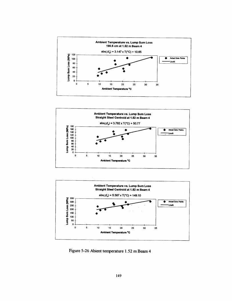

5.6 Effects of Prestress Loss on Camber and Deflection
5.6. l Introduction
Camber and deflection of prestressed members are inherently affected by the amount of
prestress force at any time, t. With the knowledge of what the prestress loss is at any time,
t, a better estimate of the time-dependent camber and deflection can be obtained. Camber
and deflection for simply-supported flexural members usually have their maximum values
occurring at the midspan.
Typically, in evaluating the equations for camber and deflection of prestressed
members, one loss value is assumed at any time and it is considered to be uniform across
the cross-section. It has been demonstrated throughout this report, that the prestress loss is
not uniform, rather, it varies within an examined cross-section. At what level should the
prestress loss within a given cross-section be used in the camber and deflection
calculations? Some examples of locations where the loss should be taken are the steel
centroid, concrete centroid, and composite centroid.
5.6.2 Field Measurement of Camber and Deflection
The Quality Control personnel, at the Hardaway Company Prestress Division,
recorded camber and deflection calculations before the girders were moved to the bridge
site. The times at which the readings were taken at the midspan are as follows:
immediately after transfer, 28, 60, and 90 days. The values obtained for the midspans
150
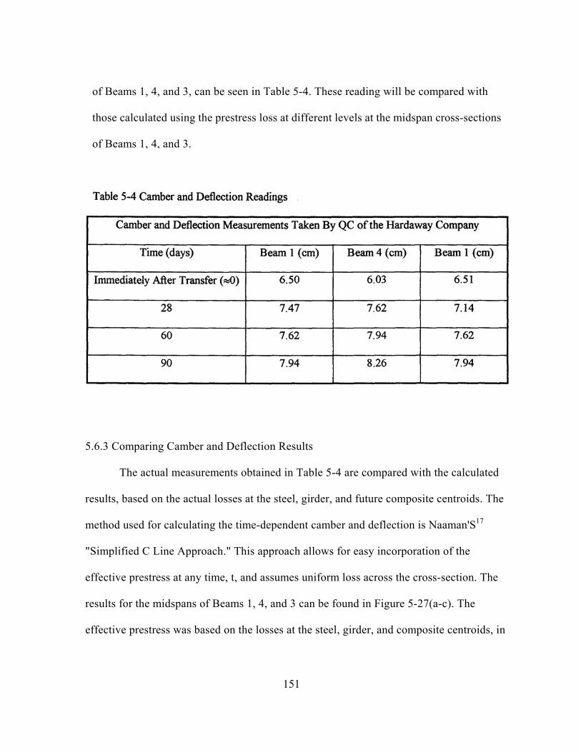
of Beams 1, 4, and 3, can be seen in Table 5-4. These reading will be compared with
those calculated using the prestress loss at different levels at the midspan cross-sections
of Beams 1, 4, and 3.
5.6.3 Comparing Camber and Deflection Results
The actual measurements obtained in Table 5-4 are compared with the calculated
results, based on the actual losses at the steel, girder, and future composite centroids. The
method used for calculating the time-dependent camber and deflection is Naaman'S17
"Simplified C Line Approach." This approach allows for easy incorporation of the
effective prestress at any time, t, and assumes uniform loss across the cross-section. The
results for the midspans of Beams 1, 4, and 3 can be found in Figure 5-27(a-c). The
effective prestress was based on the losses at the steel, girder, and composite centroids, in
151

order to see which may best model the actual measurements of camber and deflection.
From all three of these plots, the camber and deflection are best modeled after the loss
at the steel centroid.
152


APPENDIX A
ACI COMMITTEE 209 METHOD FOR DETERMINING E,(t)
In the text "Concrete Structures: Stresses and Deformations," by Ghali and Farvel8, it
suggests a few different methods for determining the time-dependent modulus of elasticity
of concrete. The method used here is that which was suggested by the ACI Committee
209.19 This committee suggests the following equation:
In Equation A- 1, E,.(to) is the modulus of elasticity of concrete at any time to, a and b are
constants based on the type of cement used, and E.(28) is the modulus of concrete at 28
days. The modulus of concrete, E,,(28), can be determined by Equation 2.1, but for high
strength concrete (fc' > 6000 psi) it will be overestimated. 20 Carrasquillo, Nilson, and Slate
suggest to use the following equation:
Equation A-2 requires fc' to be in psi and the corresponding result, Ec will also be in psi.


APPENDIX A
ACI COMMITTEE 209 METHOD FOR DETERMINING Ec(t)
In the text "Concrete Structures: Stresses and Deformations," by Ghali and Farve18, it
suggests a few different methods for determining the time-dependent modulus of elasticity
of concrete. The method used here is that which was suggested by the ACI Committee
209.19 This committee suggests the following equation:
In Equation A-1, E,-(to) is the modulus of elasticity of concrete at any tim
constants based on the type of cement used, and Ec(28) is the modulus of
The modulus of concrete, Ec(28), can be determined by Equation 2.1, but
concrete (fc' > 6000 psi) it will be overestimated.20 Carrasquillo, Nilson, a
use the following equation:
e to, a and b are
concrete at 28 days.
for high strength
nd Slate suggest to

Equation A-2 requires fc' to be in psi and the corresponding result, Ec will also be in
155

REFERENCES
'Nilson, Arthur H. Design of Prestressed Concrete. New York: John Wiley & Sons, 1987.
2PCI Committee. "Recommendations for Estimating Prestress Losses." PCI Journal July-
August 1975: 44-75.
'Lin, T. Y. and Burns, Ned H. Design of Prestressed Concrete Structures. 3rd ed. New
York: John Wiley & Sons, 1981.
4PCI Institute. PCI Design Handbook: Precast and Prestressed Concrete. 4th ed. Chicago:
1992.
5Naaman, Antoine E. Prestress Concrete Analysis and Design Fundamentals. New York:
McGraw-Hill Inc., 1982.
6Nawy, Edward G. Fundamentals of High Strength High Performance Concrete. Essex,
England: Longman Group Limited, 1996.
7Finley McNary/Janssen Spaans. State Road No. 600 Westbound Gandy Bridge (Value
Engineering Contract). Tallahassee, 1995.
BGeokon Inc. Instruction Manual: Models VCE-4200/4202/4210 Vibrating Wire Strain
Gages. Lebanon, New Hampshire: 1995.
9ACI. Building Code Requirements for Reinforced Concrete (ACI 318-89)S Revised
1992) and Commentary-ACI 318R-89 (Revised 1992,). Detroit, Michigan:
American Concrete Institute, 1992.
10Ghali, A. and Farve, R. Concrete Structures: Stresses and Deformations 2nd Edition.
London: E & FN Spon, 1994.
11CEB-FIP 1990. Model Code for Concrete Structures (MC-90). London: Thomas
Telford, 1993.
156

157