Feature extraction and tracking for scanning range sensors

Robotics and Autonomous Systems 33 (2000) 43–58

Feature extraction and tracking for scanning range sensors

N.E. PearsDepartment of Computer Science, York University, Heslington, York Y010 5DD, UK

Received 26 May 1999; received in revised form 14 February 2000Communicated by F.C.A. Groen

Abstract

A solution to the problem of simultaneously extracting and tracking a piecewise-linear range representation of a mobilerobot’s local environment is presented. The classical framework of the extended Kalman filter fits this problem extremelywell and the algorithm presented is immune to vehicle motion and active sensor reorientation during the finite capture timeof the range scan. The paper also tackles the problems of fast, non-iterative, initialisation of feature tracks, and feature trackmanagement over multiple scans. © 2000 Elsevier Science B.V. All rights reserved.

Keywords:Range sensing; Feature extraction; Feature tracking; Mobile robot navigation; Laser scanners

1. Introduction

Several different methods and numerous differentconfigurations of range sensing have been investi-gated for 3D inspection and Robotics applications [3].These include optical radar [10], sonar [6], projectedstripe [5], projected spot [9] and projected pattern[8] schemes. The latter three are based on opticaltriangulation. This provides an effective solution forshort to medium range sensing and systems can read-ily be reconfigured according to application. Indeed,a recent system has employed variable geometry toextract range maps with different qualities whichsubsequently may be fused into a single high qualitymap [18].

We have developed a scanning range sensor, basedon optical triangulation to guide obstacle avoidanceand docking manoeuvres of a mobile robot. Scanning acollimated laser beam rather than projecting a stripe, orpattern, requires extra mechanical complexity, but can

∗ E-mail address:[email protected] (N.E. Pears).

provide a more favourable signal-to-noise ratio. Also,the correspondence problem associated with projectedpatterns is obviated and, furthermore, some types ofdetector, such as the analogue lateral-effect photodi-ode, necessitate a collimated projection. Given that therange sensor is scanning over an angle which definesthe field of view, and we wish to reorient that fieldof view in order to fixate on a useful range feature,the problem then is to eliminate the distortions due tothese rapid active sensor movements and the motionof the vehicle, and track those features relative to thevehicle.

The mechatronic design of the sensor, its cali-bration, and its local processing structure have beenpresented in detail in previous papers [11,12]. Toprovide context, Appendices A and B briefly reviewsome of this work. However, the central idea pre-sented in this paper is a new feature extraction andtracking algorithm, where the features are linear seg-ments extracted from the scan. The essence of thisalgorithm is introduced in Section 2.1. The algorithmpresented is fast (minimal latency) and tracks features

0921-8890/00/$ – see front matter © 2000 Elsevier Science B.V. All rights reserved.PII: S0921-8890(00)00089-0

44 N.E. Pears / Robotics and Autonomous Systems 33 (2000) 43–58

with an accuracy and reliability which is essential forclose range avoidance manoeuvres. Other roboticsresearch using laser range scanners [16,17] has con-centrated on robot localisation within a map, whichhas a different set of sensor performance require-ments. Although our sensor system was designed forcollision avoidance, the feature extraction and track-ing algorithms presented here are also suitable formany mobile robot navigation applications such asmap building and localisation algorithms.

A requirement of the algorithm is that it permits(i.e. is robust to) vehicle motion and rotations of thesensor’s body (for active sensing). Section 2 discussesthe applicability of the extended Kalman filter and ar-gues that the algorithm presented is suitable for anyscanning range sensor which provides noisy rangemeasurements at deterministic orientations when therelative motion between sensor and scene is also noisy.Section 3 presents the detailed analysis and modellingthat is required for the algorithm. This includes a so-lution to obtaining a fast and accurate initial featurestate estimate. Section 4 discusses feature track man-agement over multiple scans, whilst Section 5 presentsresults from the extraction/tracking algorithm. Section6 discusses about extending the feature set to includeellipses.

1.1. Definition of frames of reference

The sensor used in our experiments makes a hor-izontal one-dimensional scan with a collimated laserabout aprojection axis. This scan defines the size ofthe sensor’s field of view. Also, the whole sensor bodycan rotate about the sensor axis, which allows reori-entation of the sensor field of view in the same planeas the laser scan. Due to the sensor design, the sensoraxis and projection axis are not coincident (see Ap-pendix A for more details), and it is necessary to de-fine a projection frame and sensor frame as shown in

Table 1Mobile robot reference frames

Frame Representations Tasks

Global, Og BCS location Strategic path planning, map building

Vehicle, Ov Vehicle dimensions, sensor locations Obstacle avoidance, feature extraction/tracking

Sensor,Os Calibration table Calibration

Projection,Op r, θ measurements Feature observation

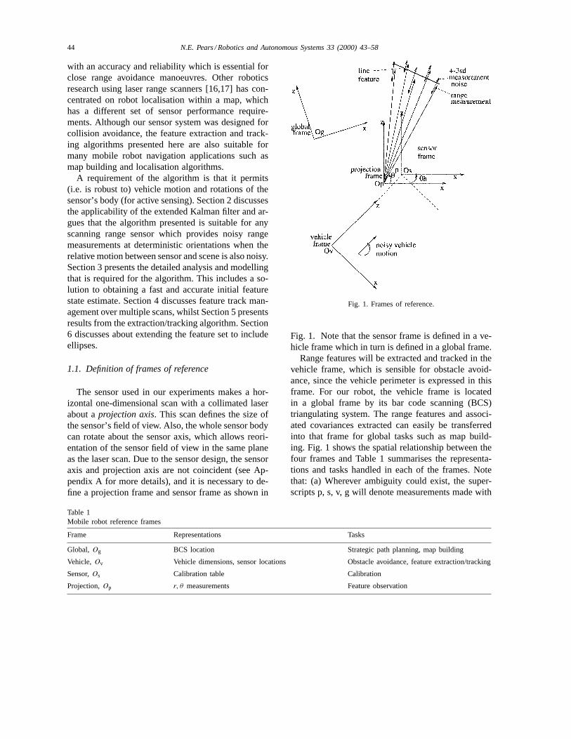
Fig. 1. Frames of reference.

Fig. 1. Note that the sensor frame is defined in a ve-hicle frame which in turn is defined in a global frame.

Range features will be extracted and tracked in thevehicle frame, which is sensible for obstacle avoid-ance, since the vehicle perimeter is expressed in thisframe. For our robot, the vehicle frame is locatedin a global frame by its bar code scanning (BCS)triangulating system. The range features and associ-ated covariances extracted can easily be transferredinto that frame for global tasks such as map build-ing. Fig. 1 shows the spatial relationship between thefour frames and Table 1 summarises the representa-tions and tasks handled in each of the frames. Notethat: (a) Wherever ambiguity could exist, the super-scripts p, s, v, g will denote measurements made with

N.E. Pears / Robotics and Autonomous Systems 33 (2000) 43–58 45

respect to one of these four frames. (b) We use the(x, z) plane in each case, they coordinate would beused if two-dimensional laser scans were employed.

2. Feature extraction and tracking using theEKF: Overview

The Kalman filter is a state estimator for linear sys-tems. When a nonlinear system is effectively modelledby linear equations (linearised), the resulting estimatoris called an extended Kalman filter. The fundamentaldifference between a standard least squares (LS) es-timator and the Kalman filter is that the former canonly be employed for the estimation of a static state,whereas the Kalman filter can estimate a dynamic state[1]. In designing a Kalman filter estimator, one needsto define (a) aprocess model(the system dynamics),which describes the evolution of the state with respectto some input(s), and subject to some processes noise,and (b) ameasurement model, which describes howmeasurements (subject to additive measurement noise)relate to the system state. The success of a particularestimator is crucially dependent on the representationsand modelling of both the system dynamics and sens-ing (measurement). The Kalman filter has been usedextensively in Robotics applications for a variety ofpurposes, such as data fusion [4] and feature tracking[2]. Here, we are particularly concerned with findinggood representations for an integrated feature extrac-tion and tracking process for scanning rangefinders.

It is assumed that the range data set for a givenscan can be associated with a piecewise linear modelof the world. For many real environments in whichautonomous vehicles operate (containing, e.g. walls,pillars and boxes) this assumption is not unrealistic.The feature extraction algorithm must estimate the pa-rameters of the line segments, the position of rangediscontinuities, and their associated uncertainties. InSection 1.1, it was pointed out that features must beextracted and tracked in the vehicle frame. This is be-cause of the following:• It removes the need for the rest of the system to

know the details of the sensor head positioning ofthe active sensor.

• It is the appropriate frame in which to use thefeatures for implementing obstacle avoidance ma-noeuvres.

• It is the appropriate frame in which to integratethe (abstracted) data from several different sensorsources in a sensor suite.We elected to examine recursive (point by point as

opposed to batch) approaches to ensure accurate com-pensation of the vehicle and sensor head motion be-tween range sample instants, and to ensure a featureset that is as up-to-date as possible. This, in additionto adding measurement to feature matching, avoids la-tency in sensor head control. An approach which isrelatively fast would be the standard formulation ofa recursive least squares (RLS) estimator. RLS couldnot be applied directly to(x, z) measurements in thesensor frame, since these two coordinates are not in-dependent, but are related through the laser scan angle(in factx needs to be deterministic). It is possible to re-move this dependence by appropriate transformationsof coordinate frames. However, we would still be leftwith an estimator that estimates a static (non-evolving)state. Clearly, for a moving vehicle, feature extractionand tracking in the vehicle frame requires estimationof a dynamic state. This implies the use of a Kalmanfilter, and since the robot/sensor system is modelledby a set of articulated rotations, it is formulated in itslinearised or extended form (EKF). A polar represen-tation of line segments (length and orientation of linenormal) is employed as this seems a natural choice ina scenario, where both the robot and sensor head canrotate. The main benefits the EKF provides are:1. The EKF’s mechanism for validating observations

provides a mean for determining range discontinu-ities (i.e. new features).

2. The process (dynamic state) in the EKF automat-ically compensates for vehicle movements duringfeature estimation.

3. The process also allows tracking of all features.(This includes those that have disappeared fromthe field of view, which gradually degrade, and un-less reobserved, are eventually removed from thetracking list.) In our application, feature tracking isused for obstacle avoidance, and repositioning ofthe sensor head.In summary, the algorithm described in Section 3

extracts and tracks polar line segments from sequencesof noisy range measurements, when the vehicle mo-tion estimate is noisy, and the orientation of the rangemeasurement relative to the robot body is assumed tobe noise free (deterministic).


2.1. Tracking features over multiple scans

The EKF process allows compensation for vehi-cle movement within a single sensor sweep, but alsoallows the localisation of features to improve acrossmultiple laser sweeps by matching individual rangemeasurements to features. This requires careful man-agement of line segment boundaries in the filter in or-der to predict feature visibility prior to association of arange measurement and feature. A feature is describedas visible at stepk if the laser projection direction ispredicted to intersect the feature within its boundarypoints (start point and end point).

Since we wish to compensate for vehicle motion asthe sensor sweeps, the EKF must cycle at the same fre-quency as range measurement are made. This meansthat the observation in the EKF can only operate ona representation of the infinite, ideal line. Boundarypoints and their derivatives, length and midpoint, arenot directly observed. However, boundary points arefundamental for vehicle and sensor head control, andare also required to predict feature visibility whenmatching new observations to features extracted fromprevious scans.

We use the state prediction of the EKF to propa-gate motion of the boundary points and their associ-ated uncertainty due to the noisy system process (ve-hicle motion). Describing a boundary point simply interms of its Cartesian coordinates does not containany information about the direction in which the linesegment was first observed. This means that it is notpossible to update the position of the boundary pointwhen observations of the infinite line segment changethe estimated polar parameters of that infinite line.

A natural way to solve this problem is to propagatethree (infinite) lines, each represented by a polar pa-rameterisation in the vehicle frame. One of these linesis the line feature, and the other two lines delimit theextent of the feature, i.e. their intersections with theline feature define the feature boundaries, which areused in feature visibility computations.

Thus, a novel feature of this algorithm is that thestate of a line segment feature isredundantlydefinedas three infinite lines, which is a redundant represen-tation since the bounding rays and line feature itselfrequire a total of six parameters to define rather thanthe four required to define end points of the line seg-ment feature. Each of the six infinite lines parame-

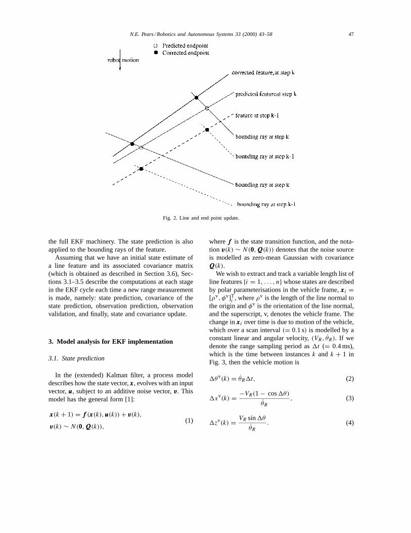
ters evolve through a predictive, noisy motion process,whereas only the two line segment parameters (not thebounding ray parameters) can be corrected ateveryrange measurement through the full EKF machinery(see Fig. 2).

Although each range reading updates an ideal line, itmay or may not update one of its associated boundingrays. If the feature is being resized (by growth or ero-sion as described in Section 4), then a bounding ray isset in the vehicle frame, and assigned zero covariancesince angular measurements of the laser projection areconsidered to be deterministic in the vehicle frame. Ifrange measurements are made (and validated) withinthe predicted bounding rays of the feature, then noobservation of a bounding ray is made. Note that theuncertainty in an unobserved bounding ray increasesat each time step due to noise in the vehicles motion(process noise).

In [17], the predictive–corrective structure of theKalman filter was employed for mobile robot localisa-tion using a range sensor, although here it is describedas a “statistical evolution uncertainty technique”. Inthis work, planar surfaces are extracted from rangedata using a method based on the Hough transform,and subsequently they are matched to predicted sur-faces from a map. In the work presented here, thereare a number of differences. Since segmentationand matching measurements to features are closelybound within the same algorithm, which is operatingat range sampling rate (rather than at frame capturerate), measurement to feature matching is taking placeat the earliest possible time. This gives two benefits:Firstly, it allows motion during the finite capture timebetween individual range measurements to be accu-rately compensated for. Secondly, it allows one tomatch every range measurement to the best possibleestimate of the tracked feature. Effectively matchingtakes place at a lower level, closer to the actual rangemeasurements, and as soon as they are made. Thisapproach can only be effective if an accurate estimateof measurement noise is available at each range sam-ple. Often, as in our case, it can be determined fromthe intensity image, as described in Appendix B and[11].

In the following section, we describe the processand measurement models for extracting and trackinglines. We describe these with reference to the ideal,infinite line, as this is the part of the state that uses


Fig. 2. Line and end point update.

the full EKF machinery. The state prediction is alsoapplied to the bounding rays of the feature.

Assuming that we have an initial state estimate ofa line feature and its associated covariance matrix(which is obtained as described in Section 3.6), Sec-tions 3.1–3.5 describe the computations at each stagein the EKF cycle each time a new range measurementis made, namely: state prediction, covariance of thestate prediction, observation prediction, observationvalidation, and finally, state and covariance update.

3. Model analysis for EKF implementation

3.1. State prediction

In the (extended) Kalman filter, a process modeldescribes how the state vector,xxx, evolves with an inputvector,uuu, subject to an additive noise vector,vvv. Thismodel has the general form [1]:

xxx(k + 1) = fff (xxx(k),uuu(k)) + vvv(k),

vvv(k) ∼ N(0,QQQ(k)),(1)

wherefff is the state transition function, and the nota-tion vvv(k) ∼ N(0,QQQ(k)) denotes that the noise sourceis modelled as zero-mean Gaussian with covarianceQQQ(k).

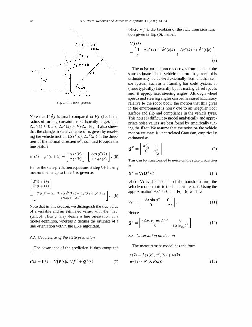
We wish to extract and track a variable length list ofline features{i = 1, . . . , n} whose states are describedby polar parameterisations in the vehicle frame,xxxi =[ρv, φv]Ti , whereρv is the length of the line normal tothe origin andφv is the orientation of the line normal,and the superscript, v, denotes the vehicle frame. Thechange inxxxi over time is due to motion of the vehicle,which over a scan interval(= 0.1 s) is modelled by aconstant linear and angular velocity,(VR, θR). If wedenote the range sampling period as1t (= 0.4 ms),which is the time between instancesk and k + 1 inFig. 3, then the vehicle motion is

1θv(k) = θR1t, (2)

1xv(k) = −VR(1 − cos1θ)

θR

, (3)

1zv(k) = VR sin1θ

θR

. (4)


Fig. 3. The EKF process.

Note that if θR is small compared toVR (i.e. if theradius of turning curvature is sufficiently large), then1xv(k) ≈ 0 and1zv(k) ≈ VR1t . Fig. 3 also showsthat the change in state variableρv is given by resolv-ing the vehicle motion(1xv(k), 1zv(k)) in the direc-tion of the normal directionφv, pointing towards theline feature:

ρv(k) − ρv(k + 1) =[

1xv(k)

1zv(k)

]·[

cosφv(k)

sinφv(k)

]. (5)

Hence the state prediction equations at stepk+1 usingmeasurements up to timek is given as[

ρv(k + 1|k)

φv(k + 1|k)

]

=[

ρv(k|k) − 1xv(k) cosφv(k|k) − 1zv(k) sinφv(k|k)

φv(k|k) − 1θv

]. (6)

Note that in this section, we distinguish the true valueof a variable and an estimated value, with the “hat”symbol. Thusφ may define a line orientation in amodel definition, whereasφ defines the estimate of aline orientation within the EKF algorithm.

3.2. Covariance of the state prediction

The covariance of the prediction is then computedas

PPP(k + 1|k) = ∇f Pf Pf P(k|k)∇fff T + QQQv(k), (7)

where∇fff is the Jacobian of the state transition func-tion given in Eq. (6), namely

∇fff (k)

=[

1 1xv(k) sinφv(k|k) − 1zv(k) cosφv(k|k)

0 1

].

(8)

The noise on the process derives from noise in thestate estimate of the vehicle motion. In general, thisestimate may be derived externally from another sen-sor system, such as a scanning bar code system, or(more typically) internally by measuring wheel speedsand, if appropriate, steering angles. Although wheelspeeds and steering angles can be measured accuratelyrelative to the robot body, the motion that this givesin the environment is noisy due to an irregular floorsurface and slip and compliance in the vehicle tyres.This noise is difficult to model analytically and appro-priate noise values are best found by empirically tun-ing the filter. We assume that the noise on the vehiclemotion estimate is uncorrelated Gaussian, empiricallyestimated as

QQQR =[

σ 2VR

00 σ 2

θR

]. (9)

This can be transformed to noise on the state predictionas

QQQv = ∇t Qt Qt QR∇tttT, (10)

where∇ttt is the Jacobian of the transform from thevehicle motion state to the line feature state. Using theapproximation1xv ≈ 0 and Eq. (6) we have

∇ttt =[ −1t sinφv 0

0 −1t

]. (11)

Hence

QQQv =[

(1tσVRsinφv)2 00 (1tσθR

)2

]. (12)

3.3. Observation prediction

The measurement model has the form

r(k) = h(xxx(k), θp, θh) + w(k),

w(k) ∼ N(0, R(k)), (13)


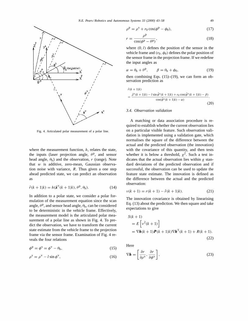
Fig. 4. Articulated polar measurement of a polar line.

where the measurement function,h, relates the state,the inputs (laser projection angle,θp, and sensorhead angle,θh) and the observation,r (range). Notethat w is additive, zero-mean, Gaussian observa-tion noise with variance,R. Thus given a one stepahead predicted state, we can predict an observationas

r(k + 1|k) = h(xxxv(k + 1|k), θp, θh). (14)

In addition to a polar state, we consider a polar for-mulation of the measurement equation since the scanangle,θp, and sensor head angle,θh, can be consideredto be deterministic in the vehicle frame. Effectively,the measurement model is the articulated polar mea-surement of a polar line as shown in Fig. 4. To pre-dict the observation, we have to transform the currentstate estimate from the vehicle frame to the projectionframe via the sensor frame. Examination of Fig. 4 re-veals the four relations

φp = φs = φv − θh, (15)

ρs = ρv − l sinφv, (16)

ρp = ρs + r0 cos(φp − φ0), (17)

r = ρp

cos(φp − θp), (18)

where(0, l) defines the position of the sensor in thevehicle frame and(r0, φ0) defines the polar position ofthe sensor frame in the projection frame. If we redefinethe input angles as

α = θh + θp, β = θh + φ0, (19)

then combining Eqs. (15)–(19), we can form an ob-servation prediction as

r(k + 1|k)

= ρv(k + 1|k) − l sinφv(k + 1|k) + r0 cos(φv(k + 1|k) − β)

cos(φv(k + 1|k) − α).

(20)

3.4. Observation validation

A matching or data association procedure is re-quired to establish whether the current observation lieson a particular visible feature. Such observation vali-dation is implemented using a validation gate, whichnormalises the square of the difference between theactual and the predicted observation (the innovation)with the covariance of this quantity, and then testswhether it is below a threshold,g2. Such a test in-dicates that the actual observation lies withing stan-dard deviations of the predicted observation and ifsuccessful, the observation can be used to update thefeature state estimate. The innovation is defined asthe difference between the actual and the predictedobservation:

ν(k + 1) = r(k + 1) − r(k + 1|k). (21)

The innovation covariance is obtained by linearisingEq. (13) about the prediction. We then square and takeexpectations to give

S(k + 1)

= E[ν2(k + 1)

]= ∇hhh(k + 1)PPP (k + 1|k)∇hhhT(k + 1) + R(k + 1).

(22)

Here

∇hhh =[

∂r

∂ρv ,∂r

∂φv

], (23)


where, in our application

∂r

∂ρv = 1

cos(φv − α), (24)

∂r

∂φv = −l cosφv − r0 sin(φv − β)

cos(φv − α)

+ (ρv − l sinφv + r0 cos(φv − β)) sin(φv−α)

cos2(φv−α).

(25)

To generateR(k + 1) = σ 2r (k + 1), the zero-mean

Gaussian noise computed for depth,z, using measuredimage position noise (Appendix B) and the calibra-tion table for image position to depth [11], must betransformed to a noise on the measured range. In theprojection frame, the scan angle is considered to bedeterministic, thus

σ 2r = σ 2

z cosec2 θp. (26)

Having computed the covariance of the innovation,association of the observation with the feature stateis achieved through a validation gate test, which isdefined by

ν2(k + 1)

S6 g2. (27)

3.5. State and covariance update

If an observation is validated by Eq. (27), themeasurement and its variance is used to update thefeature state and associated covariance matrix. Thewell-known information form of the Kalman filter [1]is used giving the state update for validated observa-tions as

xxx(k + 1|k + 1) = xxx(k + 1|k) + WWW(k + 1)ν(k + 1)

(28)

and covariance update as

PPP(k + 1|k + 1)

= PPP(k + 1|k) − WWW(k + 1)S(k + 1)WWWT(k + 1),

(29)

whereW is the Kalman gain, which is computed as

WWW(k + 1) = PPP(k + 1|k)∇hhhTS−1(k + 1). (30)

3.6. The bootstrap process

When a consecutive sequence ofn (typically five)observations are unmatched to an existing featuretrack, a new feature is instantiated. Ann point batchinitialisation process is required to provide the initialfeature state estimate,xxx(k|k), and associated covari-ance,PPP(k|k), on which the recursive process canoperate. Often, in Kalman filter implementations, avery rough estimate of the initial state is made andthe initial covariance matrix is made large, to reflectthis. Here we can compute an initial state, and itsassociated covariance as we know the variance associ-ated with each range measurement. In one approach,the problem may be formulated as a nonlinear leastsquares minimisation with [ρv, φv]T chosen to solve

[ρv, φv]T =

argminρv,φv

∑ [ri − ρv − l sinφv + r0 cos(φv − βi)

cos(φv − αi)

]2

.

(31)

However, it is not desirable to implement an iterativesolution to this equation in an algorithm which mustrun in real time. A preferable approach is transformthe problem into a more tractable linear form. As withthe recursive process, it is inappropriate to use a batchLS estimator directly to estimate the initial state, sincethe world coordinatesx andz are not independent, butare related by the scan angle. This means that errors inthe measured range will, in general, project into boththex andz coordinates. To minimise the projection oferrors into thex coordinate, which allows a standardbatch LS to be applied, the following algorithm isimplemented.

3.6.1. Initialisation algorithm1. Transform measurements [x, z]pi , i = 1, . . . , n−1,

to projection framen. This compensates for bothvehicle movements and sensor head movementsduring the initialisation process. Over the initial-isation period (typically 2 ms) the small vehiclemovement is treated as deterministic.

2. Compute the centroid, [x, z]p, of the data set inprojection framen and determine the angle,θc, ofthe centroid with respect to thezp axis of this frame.


3. Apply a rotation matrix to then initialisation pointsso that the centroid is coincident with thezp axis.

4. Compute a standard weighted least squares on thetransformed points to give a standard Cartesian(z = ax+ b) representation of the line segment.

5. Transform the above representation to a polar rep-resentation, [ρp, φp]T, in the projection frame suchthat

φp = tan−1b − θc + 12π,

ρp = zpm cos(tan−1a). (32)

6. Compute the covariance associated with this esti-mate as

PPP(k|k) =[∇hhhTRRR−1∇hhh

]−1. (33)

In the above,∇hhh is the stacked Jacobian measure-ment matrix

∇hhh =

∂r(θp1)

∂ρp

∂r(θp1)

∂φp

......

∂r(θpn)

∂ρp

∂r(θpn)

∂φp

=

1

cos(φp − θp1)

ρp tan(φp − θp1)

cos(φp − θp0)

......

1

cos(φp − θpn)

ρp tan(φp − θpn)

cos(φp − θpn)

(34)

andRRR is a diagonal matrix of observation variances

RRR =

σ 2r1

. . . 0...

. . ....

0 . . . σ 2rn

. (35)

7. Transform the projection frame state into the vehi-cle frame state using

ρv = ρp − r0 cos(φp − φ0)

+l sin(φp + θh), (36)

φv = φp + θh. (37)

8. Finally, transform the projection frame covarianceto the vehicle frame covariance:

PPP v = ∇uPuPuP p∇uuuT, (38)

where∇uuu is the Jacobian of the transform betweenthe projection frame and the vehicle frame

∇uuu =[

1 r0 sin(φp − φ0) − l cos(φp + θh)

0 1

].

(39)

4. Feature track management

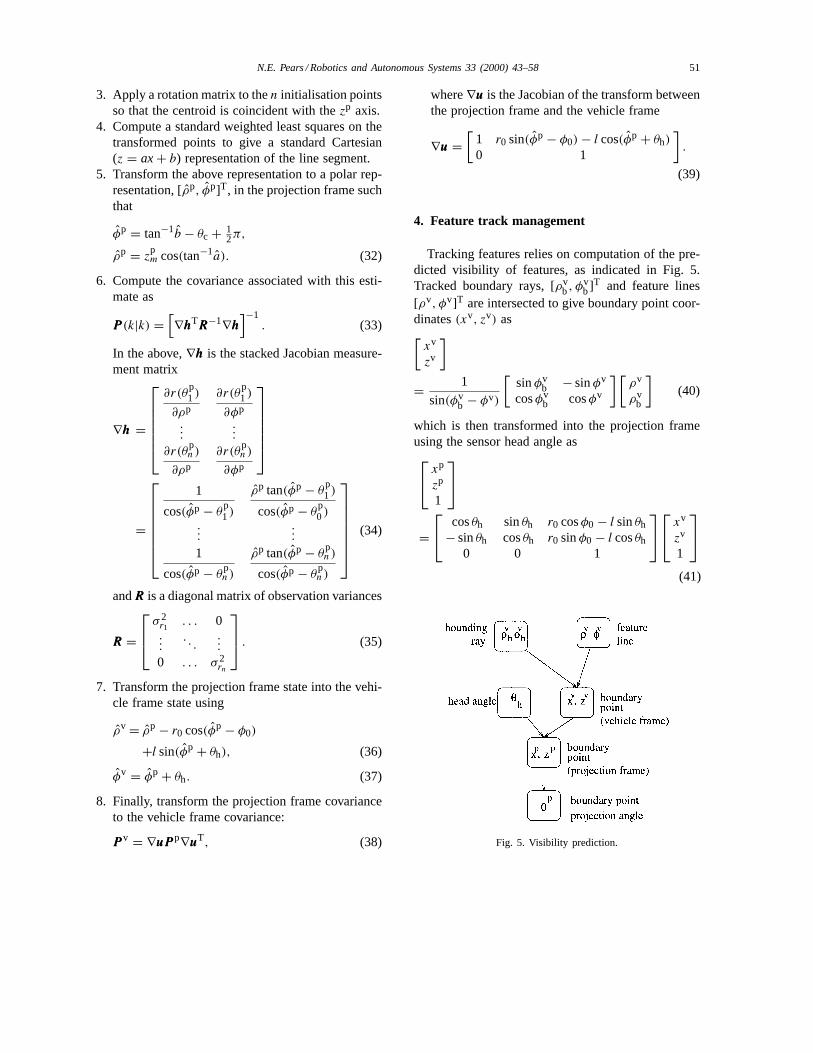
Tracking features relies on computation of the pre-dicted visibility of features, as indicated in Fig. 5.Tracked boundary rays, [ρv

b, φvb]T and feature lines

[ρv, φv]T are intersected to give boundary point coor-dinates(xv, zv) as[

xv

zv

]

= 1

sin(φvb − φv)

[sinφv

b − sinφv

cosφvb cosφv

] [ρv

ρvb

](40)

which is then transformed into the projection frameusing the sensor head angle as xp

zp

1

= cosθh sinθh r0 cosφ0 − l sinθh

− sinθh cosθh r0 sinφ0 − l cosθh0 0 1

xv

zv

1

(41)

Fig. 5. Visibility prediction.


and finally transformed into a visibility angle in theprojection frame, as illustrated in Fig. 5.

For each laser projection angle, an attempt to matchthe range measurement to visible features along thatray is made. In the simplest case, an observation ismade within the predicted visibility angle of the fea-ture and is matched (validated) to that feature, thenthe parameters and associated covariances of the infi-nite feature line are updated in the EKF framework.Multiple matches may be found as occlusion is notexplicitly modelled. In such cases the match with thesmallest innovation is chosen.

Beyond this simplest case, feature track manage-ment is required. (We refer to a feature track as theevolution of the redundant six-dimensional featurestate over multiple scans.) This entails the additionand removal of features from the tracking list, andmanages the features boundaries (start points andend points), as defined by the tracked bounding rays.Feature track management employs six specific oper-ations, described below, which can be conceptuallypaired as three operation/inverse pairs: add–delete,grow–erode, and split–merge.• Feature add. When a consecutive sequence ofn

(typically five) observations are unmatched to anexisting feature track, a new feature is instantiated.This occurs when there are either no visible features,or, for all visible features, the validation gate testfor data to track matching fails.

• Feature delete. When either of the infinite line fea-ture variances (σ 2

ρ , σ 2φ ) exceeds a threshold, the fea-

ture is deleted. (Other heuristic refinements may bemade, such as deleting features below a minimumlength, above a maximum product ofσρσφ , or abovea maximum range from the vehicle.)

• Feature grow. When observations are matched be-yond, but consecutive to the feature end point, thefeature grows from that end point. This requiresthat the system attempts a feature match to featureswhich have become invisible over the last incrementof projection angle.

• Feature erode. When observations are not matchedto a visible feature immediately after, and consecu-tive to, the feature start point, the feature is erodedat the start point. Also, when observations fail tomatch within the scan anglen dθp from the endpoint (wheredθp is the laser projection angle step),the feature is eroded at the end point.

• Feature split. If, after a sequence of matched obser-vations, a match fails before the scan angle is withinn dθp of the feature end point, the feature splits intotwo “child” features, which have the same ideal lineparameters, but different boundary points.

• Feature merge. When two features are visible at aparticular scan angle (or the previous scan angle ifa feature is growing), and the observation matchesboth feature tracks, then a check is made to see ifthe two features can be merged. This is possible iftheir parameters (of the ideal line) and associatedvariances overlap in bothρ andφ space. If sufficientoverlap is found, they are merged by weighting thetwo sets of infinite line parameters according to theirvariances, and selecting the appropriate boundarypoints. Typically, this occurs when a feature needsto grow, but in the opposite direction to the scanningmotion.

5. Performance results

The performance of the system is dependent on thelevel of noise entering the system. It seems that vehicleorientation noise has a bigger detrimental effect thantranslation noise. If the estimation of vehicle motionis noisy (e.g. if odometry only is used), then it is likelythat less matches between range measurements andfeatures will be made. However, the level of motionnoise must be included in the EKF. If this is high,then unmatched feature tracks are quickly deleted, andthe robots estimate of its immediate environment isessentially what it has seen over the last few scans.

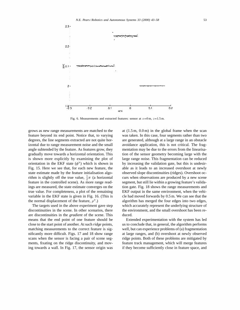
To test the performance of our algorithms, we usedthe detailed sensor simulation presented in [13], whichgives noisy range scans which are virtually indistin-guishable from our sensor. This allows us to use con-trolled scenes with known ground truth. In our firstexperiment, the line segments extracted from a scene,with low reflectivity targets parallel to the sensor, aresuperimposed on the measured points, and plotted inFig. 6. Here the sensor frame origin and vehicle frameorigin are coincident and the results are plotted in aglobal frame.

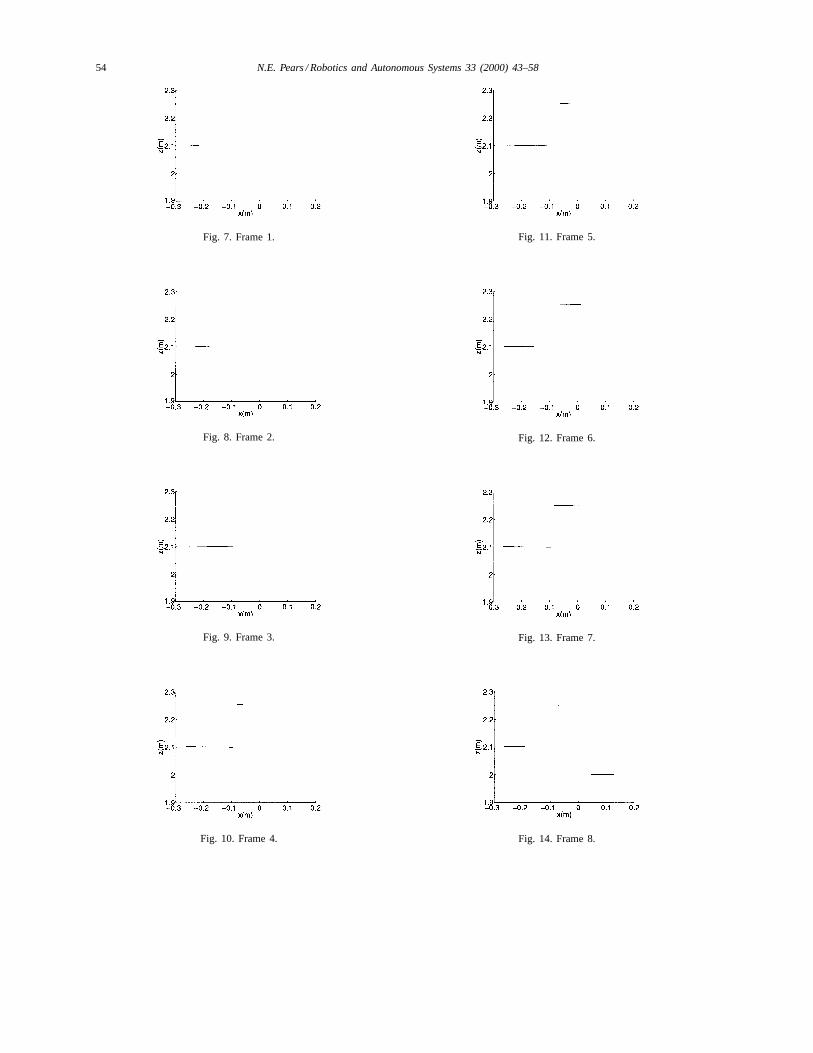
The growth of these line segments is plotted in asequence of frames shown in Figs. 7–14 as the sen-sor makes its initial scan. In this sequence of figures,we see three new features instantiated, each of which


Fig. 6. Measurements and extracted features: sensor atx=0 m, z=1.5 m.

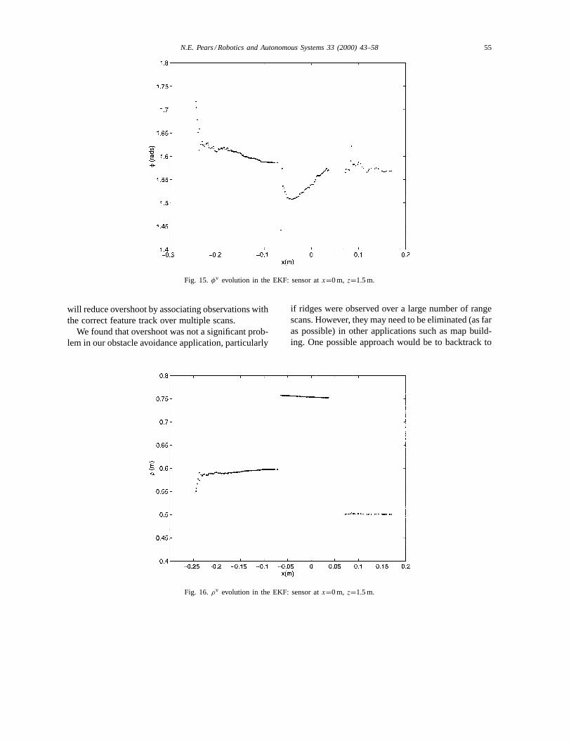
grows as new range measurements are matched to thefeature beyond its end point. Notice that, to varyingdegrees, the line segments extracted are not quite hor-izontal due to range measurement noise and the smallangle subtended by the feature. As features grow, theygradually move towards a horizontal orientation. Thisis shown more explicitly by examining the plot oforientation in the EKF state (φv) which is shown inFig. 15. Here we see that, for each new feature, thestate estimate made by the feature initialisation algo-rithm is slightly off the true value,12π (a horizontalfeature in the controlled scene). As more range read-ings are measured, the state estimate converges on thetrue value. For completeness, a plot of the remainingvariable in the EKF state is given in Fig. 16. (This isthe normal displacement of the feature,ρv.)

The targets used in the above experiment gave stepdiscontinuities in the scene. In other scenarios, thereare discontinuities in thegradientof the scene. Thismeans that the end point of one feature should beclose to the start point of another. At suchridgepoints,matching measurements to the correct feature is sig-nificantly more difficult. Figs. 17 and 18 show rangescans when the sensor is facing a pair of scene seg-ments, fixating on the ridge discontinuity, and mov-ing towards a wall. In Fig. 17, the sensor origin was

at (1.5 m, 0.0 m) in the global frame when the scanwas taken. In this case, four segments rather than twoare generated, although at a large range in an obstacleavoidance application, this is not critical. The frag-mentation may be due to the errors from the linearisa-tion of the sensor geometry becoming large with thelarge range noise. This fragmentation can be reducedby increasing the validation gate, but this is undesir-able as it leads to an increased overshoot at newlyobserved slope discontinuities (ridges). Overshoot oc-curs when observations are produced by a new scenesegment, but still lie within a growing feature’s valida-tion gate. Fig. 18 shows the range measurements andEKF output in the same environment, when the vehi-cle had moved forwards by 0.5 m. We can see that thealgorithm has merged the four edges into two edges,which accurately represent the underlying structure ofthe environment, and the small overshoot has been re-duced.

Extended experimentation with the system has ledus to conclude that, in general, the algorithm performswell, but can experience problems of (a) fragmentationat large ranges, and (b) overshoot at newly observedridge points. Both of these problems are mitigated byfeature track management, which will merge featuresif they become sufficiently close in feature space, and


Fig. 7. Frame 1.

Fig. 8. Frame 2.

Fig. 9. Frame 3.

Fig. 10. Frame 4.

Fig. 11. Frame 5.

Fig. 12. Frame 6.

Fig. 13. Frame 7.

Fig. 14. Frame 8.


Fig. 15.φv evolution in the EKF: sensor atx=0 m, z=1.5 m.

will reduce overshoot by associating observations withthe correct feature track over multiple scans.

We found that overshoot was not a significant prob-lem in our obstacle avoidance application, particularly

Fig. 16.ρv evolution in the EKF: sensor atx=0 m, z=1.5 m.

if ridges were observed over a large number of rangescans. However, they may need to be eliminated (as faras possible) in other applications such as map build-ing. One possible approach would be to backtrack to


Fig. 17. Measurements and extracted features: sensor atx=1.5 m,z=0.0 m.

a previously saved state to remove the offending out-lier(s), correct for vehicle motion in the backtrack pe-riod, and, if necessary, reconstruct the ridge points byintersection of extracted line features either side of theridge.

6. Discussion: Extending the EKF to ellipses

A possible extension to this algorithm is to aug-ment the feature set, so that the environment can be

Fig. 18. Measurements and extracted features: sensor atx=1.5 m,z=0.5 m.

modelled as set of planes and cylinders. The rangeprofile of a cylinder is circular if the cylinder is verti-cal, and elliptical, otherwise. Since circles are a sub-set of ellipses, the natural extension from exclusivelypiecewise-linear features is to allow for elliptical sec-tions. In the batch initialisation process, the appropri-ate model (linear/elliptical) which best fits the initiali-sation data could be selected, and the associated EKFmeasurement equation would be employed for the re-cursive stage of the algorithm. Unfortunately, the batchstage requires LS fitting of the standard bi-quadraticconic equation [15,19] over small sections of data.This is very ill-conditioned [14]: small changes in therange measurements can change the fit from an ellipseto a parabola or hyperbola, and the observation pre-diction has a large variance. This leads us to believethat a multi-feature set algorithm would be more suit-able to a pre-segmented batch scheme. As a conse-quence, significant latency could be introduced in thehead control. In the EKF algorithm described, ellip-tical profiles are broken down into a set of line seg-ments. Although this does not accurately reflect theunderlying structure of the environment, this situationcan be detected as the discontinuities extracted willnot exhibit predictable behaviour when the vehicle andsensor head move.

7. Conclusions

A line segment extraction and tracking algorithmhas been developed based on the EKF. The EKFprocess models the effect of (noisy) vehicle motionon a polar line representation. The EKF measure-ment model models the articulated polar observationof the polar line state. Choosing this representationhas given trivial line orientation (φ) computationsbut more complex computations for the line normal(ρ). A key idea introduced is the use of a redundantrepresentation of line features, such that a featureis represented by a polar feature line and a pair ofpolar bounding lines. This preserves informationabout the direction in which feature end points wereobserved, which is instrumental in accurate pre-diction of feature observability. The paper has alsodescribed a fast feature track initialisation procedureand has detailed a number feature track managementoperations.


A.1. Plan view of the sensor head.

Extended experimentation with the system has ledus to conclude that, in general, the algorithm performswell, and problems of fragmentation and overshootare mitigated by feature track management. Also, ifnecessary, overshoot may be eliminated by heuristicprocedures, which “fine tune” the algorithm.

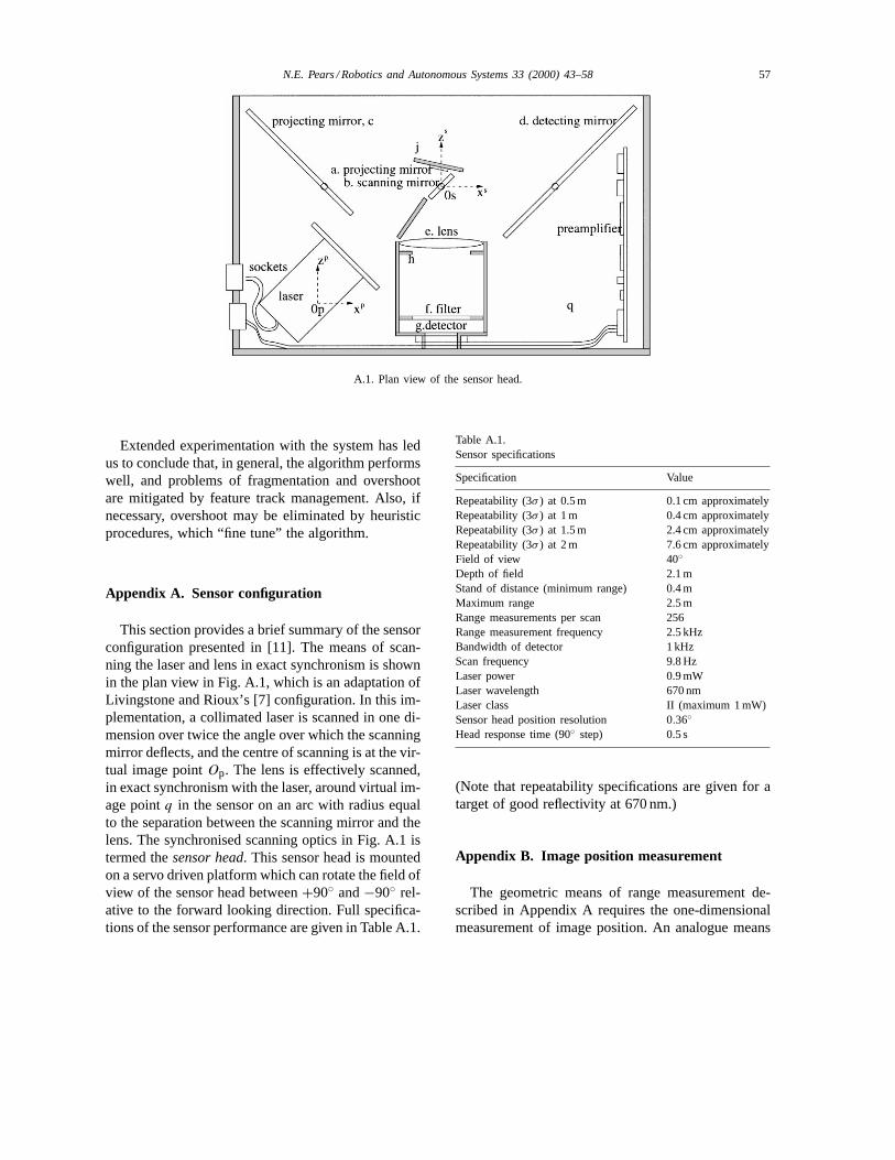
Appendix A. Sensor configuration

This section provides a brief summary of the sensorconfiguration presented in [11]. The means of scan-ning the laser and lens in exact synchronism is shownin the plan view in Fig. A.1, which is an adaptation ofLivingstone and Rioux’s [7] configuration. In this im-plementation, a collimated laser is scanned in one di-mension over twice the angle over which the scanningmirror deflects, and the centre of scanning is at the vir-tual image pointOp. The lens is effectively scanned,in exact synchronism with the laser, around virtual im-age pointq in the sensor on an arc with radius equalto the separation between the scanning mirror and thelens. The synchronised scanning optics in Fig. A.1 istermed thesensor head. This sensor head is mountedon a servo driven platform which can rotate the field ofview of the sensor head between+90◦ and−90◦ rel-ative to the forward looking direction. Full specifica-tions of the sensor performance are given in Table A.1.

Table A.1.Sensor specifications

Specification Value

Repeatability (3σ ) at 0.5 m 0.1 cm approximatelyRepeatability (3σ ) at 1 m 0.4 cm approximatelyRepeatability (3σ ) at 1.5 m 2.4 cm approximatelyRepeatability (3σ ) at 2 m 7.6 cm approximatelyField of view 40◦Depth of field 2.1 mStand of distance (minimum range) 0.4 mMaximum range 2.5 mRange measurements per scan 256Range measurement frequency 2.5 kHzBandwidth of detector 1 kHzScan frequency 9.8 HzLaser power 0.9 mWLaser wavelength 670 nmLaser class II (maximum 1 mW)Sensor head position resolution 0.36◦Head response time (90◦ step) 0.5 s

(Note that repeatability specifications are given for atarget of good reflectivity at 670 nm.)

Appendix B. Image position measurement

The geometric means of range measurement de-scribed in Appendix A requires the one-dimensionalmeasurement of image position. An analogue means


of measurement is provided by a two-terminal devicecalled the lateral-effect photodiode (LEP) which actsas a photocurrent divider so that the position of thelight, p, from the centre of a detector of length,P , is

p = I1 − I2

I1 + I2

(P

2

), −1

2P 6 p 6 +12P (B.1)

and the detector current,I0, is the sum of the terminalcurrents,I1 and I2. A previous analysis [11] estab-lished a relationship between the standard deviationassociated with an image position measurement andthe detector current for that measurement as

σpn = σp

12P

= In

I0. (B.2)

Hence, if we determineIn from calibration experi-ments, then every time a measurement is made, imageposition variance can be computed using the signalstrength,I0. This can be scaled by (the square of) thetriangulation gain, which is the magnitude of the localgradient,|∂z/∂p|z,θ in the calibration table to give anestimate of range variance. This variance informationis essential to allow robust algorithms to be applied tothe raw range data. In particular, it is used in theextended Kalman filter algorithm for simultaneousfeature extraction and tracking.

References

[1] Y. Bar-Shalom, X. Li, Estimation and Tracking: Principles,Techniques and Software, Artech House, Boston, MA, 1993.

[2] R. Deriche, O. Faugeras, Tracking line segments, Image andVision Computing 8 (4) (1990) 261–270.

[3] H.R. Everett, Survey of collision avoidance and rangingsensors for mobile robots, Robotics and Autonomous Systems5 (1989) 5–67.

[4] J. Horn, J. Neira, J.D. Tardos, G. Schmidt, Fusing rangeand intensity images for mobile robot localisation, IEEETransactions on Robotics and Automation 15 (1) (1999) 76–84.

[5] T. Kanade, A. Gruss, L.R. Carley, A very fast VLSIrangefinder, in: Proceedings of the IEEE InternationalConference on Robotics and Automation, Sacramento, CA,1991.

[6] R. Kuc, A spatial sampling criterion for sonar obstacledetection, IEEE Transactions on Pattern Analysis andMachine Intelligence 12 (7) (1990) 686–690.

[7] F.R. Livingstone, M. Rioux, Development of a large field ofview 3D vision system, SPIE Proceedings 665 (1986) 188–194.

[8] H.R. Lo, A. Blake, D. McCowen, D. Konash, Epipolargeometry for trinocular active range sensors, in: Proceedingsof the British Machine Vision Conference, 1990.

[9] J.A. Marszalec, H.M. Keranen, A photoelectric range scannerusing an array of led chips, in: Proceedings of the 1992 IEEEInternational Conference on Robotics and Automation, Nice,France, 1992, pp. 593–598.

[10] G.L. Miller, E.R. Wagner, An optical rangefinder forautonomous robot cart navigation, SPIE Proceedings 852(1987) 122–134.

[11] N.E. Pears, P.J. Probert, An intelligent active range sensor formobile robot guidance, Mechatronics 6 (7) (1996) 733–759.

[12] N.E. Pears, An intelligent active range sensor for vehicleguidance, in: Proceedings of the IEEE/RSJ InternationalConference on Intelligent Robots and Systems, Osaka, Japan,1996, pp. 81–88.

[13] N.E. Pears, Modelling of a scanning laser range sensorfor robotic applications, Advanced Robotics 13 (5) (1999)549–562.

[14] J. Porrill, Fitting ellipses and predicting confidence envelopesusing a bias corrected Kalman filter, Image and VisionComputing 8 (1) (1990) 37–41.

[15] P.L. Rosin, A note on the least squares fitting of ellipses,Pattern Recognition Letters 14 (10) (1993) 799–808.

[16] B. Schiele, J.L. Crowley, F. Wallner, Position estimationusing principal components of range data, Robotics andAutonomous Systems 23 (4) (1998) 267–276.

[17] G. Schmidt, J. Horn, Continuous localization of a mobilerobot based on 3D-laser-range-data, predicted sensor images,and dead-reckoning, Robotics and Autonomous Systems14 (2/3) (1995) 99–118.

[18] A.M. Wallace, J. Clark, G.C. Pronzato, Measuring rangeusing a triangulation sensor with variable geometry, IEEETransactions on Robotics and Automation 14 (1) (1998)60–68.

[19] W.Y. Wu, Elliptical object detection by using its geometricproperties, Pattern Recognition 26 (10) (1993) 1499–1509 .

Nick Pears was awarded a B.Sc. in Engi-neering Science, and a Ph.D. in Robotics,1990, by Durham University, UK. He thenundertook post-doctoral research in the“Sensors and Architectures” division of theRobotics Research Group, Oxford Univer-sity. In 1994, he was elected as a Col-lege Lecturer and Fellow of Girton Col-lege, Cambridge University. In 1998, hejoined the Computer Science Department,

University of York, UK, in his current Lectureship. His researchinterests are in Robotics and Computer Vision and include opticalsensor design, theoretical modelling of sensors, recursive range fea-ture extraction under motion, real-time architectures for robotics,vehicle guidance using visual cues, human–computer interactionand digital media applications of vision.

Documents

Feature extraction and tracking for scanning range sensors