Embed Size (px)
Citation preview
FATIMA MICHAEL COLLEGE OF ENGINEERING & TECHNOLOGYSenkottai Village, Madurai – Sivagangai Main Road,
Madurai - 625 020.[An ISO 9001:2008 Certified Institution]
LECTURE NOTES
EC 2029 – DIGITAL IMAGE PROCESSING
SEMESTER: VII / ECE PREPARED BY: C. Rajadurai , AP / ECE.
UNIT 1
DIGITAL IMAGE FUDAMENTALS
Digital image representation:
Digital image is a finite collection of discrete samples (pixels) of any observable object. Thepixels represent a two- or higher dimensional “view” of the object, each pixel having its owndiscrete value in a finite range. The pixel values may represent the amount of visible light, infrared light, electrons, or any other measurable value such as ultrasound wave impulses. The imagedoes not need to have any visual sense; it is sufficient that the samples form a two-dimensionalspatial structure that may be illustrated as an image.
The images may be obtained by a digital camera, scanner, electron microscope, ultrasoundstethoscope, or any other optical or non-optical sensor. Examples of digital image are:
digital photographs
satellite images
radiological images (x-rays, mammograms)
binary images, fax images, engineering drawings
Computer graphics, CAD drawings, and vector graphics in general are not considered in thiscourse even though their reproduction is a possible source of an image. In fact, one goal ofintermediate level image processing may be to reconstruct a model (e.g. vector representation)for a given digital image.
Digitization:
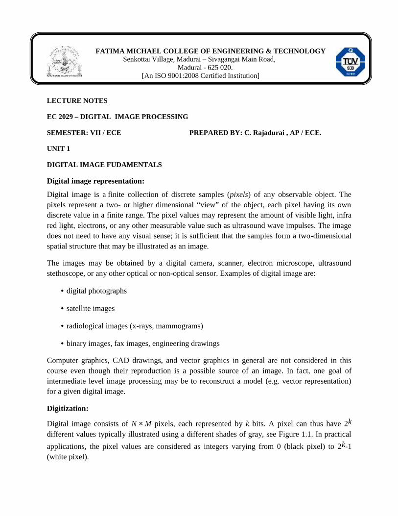
Digital image consists of N M pixels, each represented by k bits. A pixel can thus have 2k
different values typically illustrated using a different shades of gray, see Figure 1.1. In practical
applications, the pixel values are considered as integers varying from 0 (black pixel) to 2k-1(white pixel).
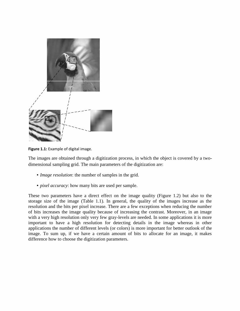
Figure 1.1: Example of digital image.
The images are obtained through a digitization process, in which the object is covered by a two-dimensional sampling grid. The main parameters of the digitization are:
Image resolution: the number of samples in the grid.
pixel accuracy: how many bits are used per sample.
These two parameters have a direct effect on the image quality (Figure 1.2) but also to thestorage size of the image (Table 1.1). In general, the quality of the images increase as theresolution and the bits per pixel increase. There are a few exceptions when reducing the numberof bits increases the image quality because of increasing the contrast. Moreover, in an imagewith a very high resolution only very few gray-levels are needed. In some applications it is moreimportant to have a high resolution for detecting details in the image whereas in otherapplications the number of different levels (or colors) is more important for better outlook of theimage. To sum up, if we have a certain amount of bits to allocate for an image, it makesdifference how to choose the digitization parameters.
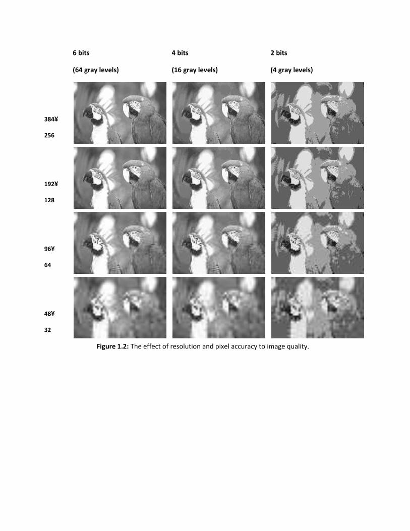
6 bits
(64 gray levels)
4 bits
(16 gray levels)
2 bits
(4 gray levels)
384
256
192
128
96
64
48
32
Figure 1.2: The effect of resolution and pixel accuracy to image quality.
6 bits
(64 gray levels)
4 bits
(16 gray levels)
2 bits
(4 gray levels)
384
256
192
128
96
64
48
32
Figure 1.2: The effect of resolution and pixel accuracy to image quality.
6 bits
(64 gray levels)
4 bits
(16 gray levels)
2 bits
(4 gray levels)
384
256
192
128
96
64
48
32
Figure 1.2: The effect of resolution and pixel accuracy to image quality.
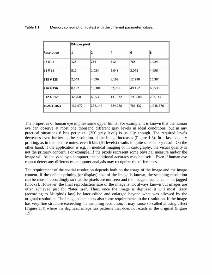
Table 1.1 Memory consumption (bytes) with the different parameter values.
Bits per pixel:
Resolution 1 2 4 6 8
32 32 128 256 512 768 1,024
64 64 512 1,024 2,048 3,072 4,096
128 128 2,048 4,096 8,192 12,288 16,384
256 256 8,192 16,384 32,768 49,152 65,536
512 512 32,768 65,536 131,072 196,608 262,144
1024 1024 131,072 262,144 524,288 786,432 1,048,576
The properties of human eye implies some upper limits. For example, it is known that the humaneye can observe at most one thousand different gray levels in ideal conditions, but in anypractical situations 8 bits per pixel (256 gray level) is usually enough. The required levelsdecreases even further as the resolution of the image increases (Figure 1.3). In a laser qualityprinting, as in this lecture notes, even 6 bits (64 levels) results in quite satisfactory result. On theother hand, if the application is e.g. in medical imaging or in cartography, the visual quality isnot the primary concern. For example, if the pixels represent some physical measure and/or theimage will be analyzed by a computer, the additional accuracy may be useful. Even if human eyecannot detect any differences, computer analysis may recognize the differences.
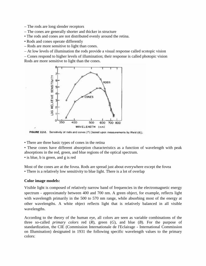
The requirement of the spatial resolution depends both on the usage of the image and the imagecontent. If the default printing (or display) size of the image is known, the scanning resolutioncan be chosen accordingly so that the pixels are not seen and the image appearance is not jagged(blocky). However, the final reproduction size of the image is not always known but images areoften achieved just for “later use”. Thus, once the image is digitized it will most likely(according to Murphy’s law) be later edited and enlarged beyond what was allowed by theoriginal resolution. The image content sets also some requirements to the resolution. If the imagehas very fine structure exceeding the sampling resolution, it may cause so-called aliasing effect(Figure 1.4) where the digitized image has patterns that does not exists in the original (Figure1.5).
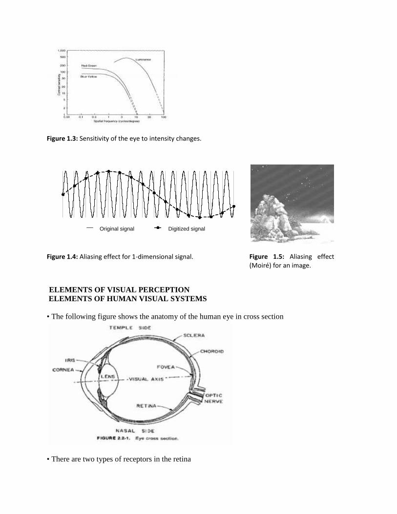
Figure 1.3: Sensitivity of the eye to intensity changes.
Original signal Digitized signal
Figure 1.4: Aliasing effect for 1-dimensional signal. Figure 1.5: Aliasing effect(Moiré) for an image.
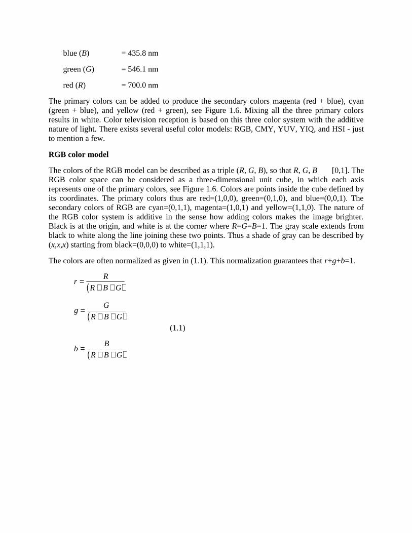
ELEMENTS OF VISUAL PERCEPTIONELEMENTS OF HUMAN VISUAL SYSTEMS
• The following figure shows the anatomy of the human eye in cross section
• There are two types of receptors in the retina
Figure 1.3: Sensitivity of the eye to intensity changes.
Original signal Digitized signal
Figure 1.4: Aliasing effect for 1-dimensional signal. Figure 1.5: Aliasing effect(Moiré) for an image.
ELEMENTS OF VISUAL PERCEPTIONELEMENTS OF HUMAN VISUAL SYSTEMS
• The following figure shows the anatomy of the human eye in cross section
• There are two types of receptors in the retina
– The rods are long slender receptors– The cones are generally shorter and thicker in structure• The rods and cones are not distributed evenly around the retina.• Rods and cones operate differently– Rods are more sensitive to light than cones.– At low levels of illumination the rods provide a visual response called scotopic vision– Cones respond to higher levels of illumination; their response is called photopic visionRods are more sensitive to light than the cones.
• There are three basic types of cones in the retina• These cones have different absorption characteristics as a function of wavelength with peakabsorptions in the red, green, and blue regions of the optical spectrum.• is blue, b is green, and g is red
Most of the cones are at the fovea. Rods are spread just about everywhere except the fovea• There is a relatively low sensitivity to blue light. There is a lot of overlap
Color image models:
Visible light is composed of relatively narrow band of frequencies in the electromagnetic energyspectrum - approximately between 400 and 700 nm. A green object, for example, reflects lightwith wavelength primarily in the 500 to 570 nm range, while absorbing most of the energy atother wavelengths. A white object reflects light that is relatively balanced in all visiblewavelengths.
According to the theory of the human eye, all colors are seen as variable combinations of thethree so-called primary colors red (R), green (G), and blue (B). For the purpose ofstandardization, the CIE (Commission Internationale de l'Eclairage - International Commissionon Illumination) designated in 1931 the following specific wavelength values to the primarycolors:
blue (B) = 435.8 nm
green (G) = 546.1 nm
red (R) = 700.0 nm
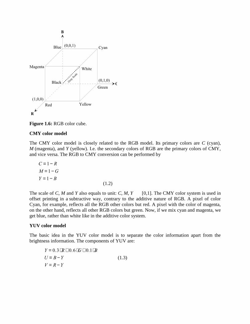
The primary colors can be added to produce the secondary colors magenta (red + blue), cyan(green + blue), and yellow (red + green), see Figure 1.6. Mixing all the three primary colorsresults in white. Color television reception is based on this three color system with the additivenature of light. There exists several useful color models: RGB, CMY, YUV, YIQ, and HSI - justto mention a few.
RGB color model
The colors of the RGB model can be described as a triple (R, G, B), so that R, G, B [0,1]. TheRGB color space can be considered as a three-dimensional unit cube, in which each axisrepresents one of the primary colors, see Figure 1.6. Colors are points inside the cube defined byits coordinates. The primary colors thus are red=(1,0,0), green=(0,1,0), and blue=(0,0,1). Thesecondary colors of RGB are cyan=(0,1,1), magenta=(1,0,1) and yellow=(1,1,0). The nature ofthe RGB color system is additive in the sense how adding colors makes the image brighter.Black is at the origin, and white is at the corner where R=G=B=1. The gray scale extends fromblack to white along the line joining these two points. Thus a shade of gray can be described by(x,x,x) starting from black=(0,0,0) to white=(1,1,1).
The colors are often normalized as given in (1.1). This normalization guarantees that r+g+b=1.
r
R
R B G
g
G
R B G
(1.1)
b
B
R B G
Cyan
YellowRed
WhiteMagenta
Blue
BlackGreen
(0,1,0)
(0,0,1)
(1,0,0)
GrayScal
e
R
G
B
Figure 1.6: RGB color cube.
CMY color model
The CMY color model is closely related to the RGB model. Its primary colors are C (cyan),M (magenta), and Y (yellow). I.e. the secondary colors of RGB are the primary colors of CMY,and vice versa. The RGB to CMY conversion can be performed by
C RM GY B
11
1(1.2)
The scale of C, M and Y also equals to unit: C, M, Y [0,1]. The CMY color system is used inoffset printing in a subtractive way, contrary to the additive nature of RGB. A pixel of colorCyan, for example, reflects all the RGB other colors but red. A pixel with the color of magenta,on the other hand, reflects all other RGB colors but green. Now, if we mix cyan and magenta, weget blue, rather than white like in the additive color system.
YUV color model
The basic idea in the YUV color model is to separate the color information apart from thebrightness information. The components of YUV are:
Y R G BU B YV R Y
0 3 0 6 0 1. . .(1.3)
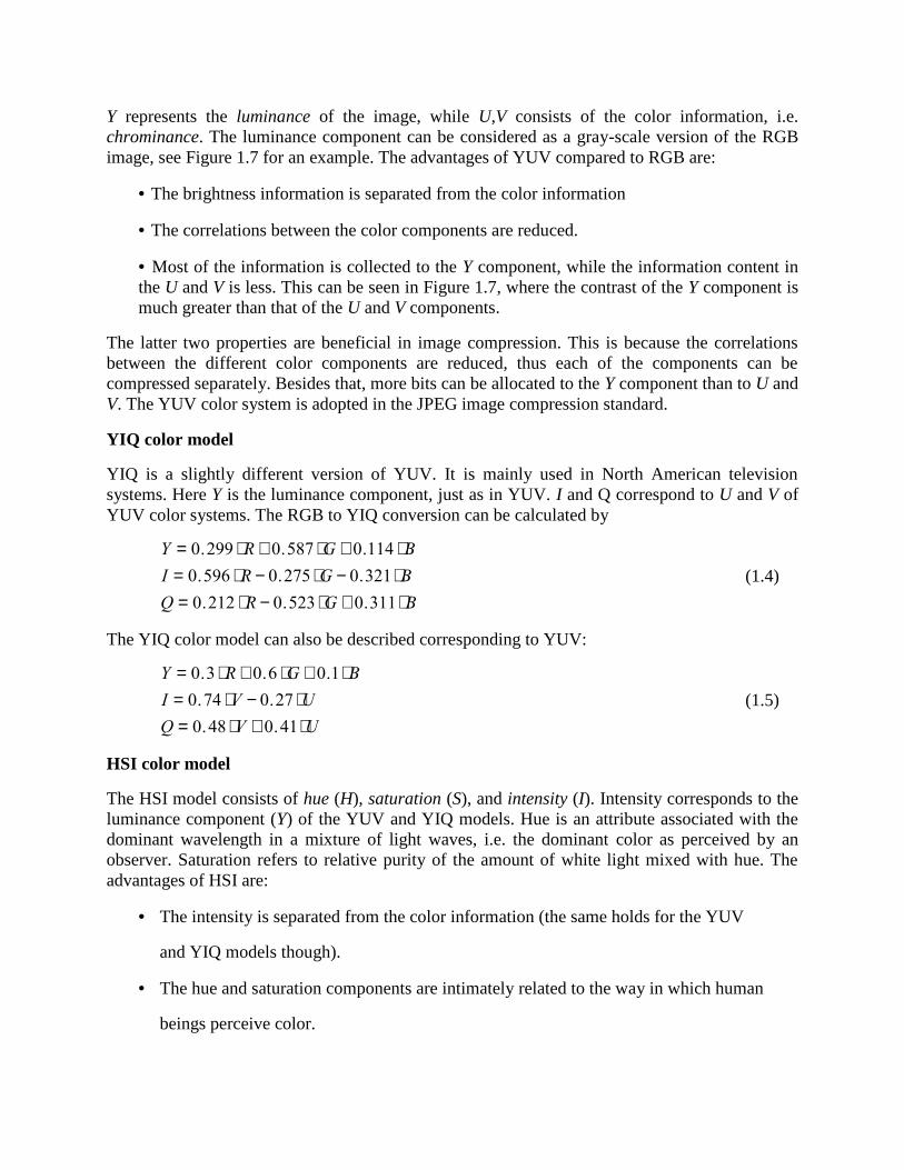
Y represents the luminance of the image, while U,V consists of the color information, i.e.chrominance. The luminance component can be considered as a gray-scale version of the RGBimage, see Figure 1.7 for an example. The advantages of YUV compared to RGB are:
The brightness information is separated from the color information
The correlations between the color components are reduced.
Most of the information is collected to the Y component, while the information content inthe U and V is less. This can be seen in Figure 1.7, where the contrast of the Y component ismuch greater than that of the U and V components.
The latter two properties are beneficial in image compression. This is because the correlationsbetween the different color components are reduced, thus each of the components can becompressed separately. Besides that, more bits can be allocated to the Y component than to U andV. The YUV color system is adopted in the JPEG image compression standard.
YIQ color model
YIQ is a slightly different version of YUV. It is mainly used in North American televisionsystems. Here Y is the luminance component, just as in YUV. I and Q correspond to U and V ofYUV color systems. The RGB to YIQ conversion can be calculated by
Y R G BI R G BQ R G B
0 299 0 587 0 1140 596 0 275 0 3210 212 0 523 0 311
. . .. . .. . .
(1.4)
The YIQ color model can also be described corresponding to YUV:
Y R G BI V UQ V U
0 3 0 6 0 10 74 0 270 48 0 41
. . .. .. .
(1.5)
HSI color model
The HSI model consists of hue (H), saturation (S), and intensity (I). Intensity corresponds to theluminance component (Y) of the YUV and YIQ models. Hue is an attribute associated with thedominant wavelength in a mixture of light waves, i.e. the dominant color as perceived by anobserver. Saturation refers to relative purity of the amount of white light mixed with hue. Theadvantages of HSI are:
The intensity is separated from the color information (the same holds for the YUV
and YIQ models though).
The hue and saturation components are intimately related to the way in which human
beings perceive color.
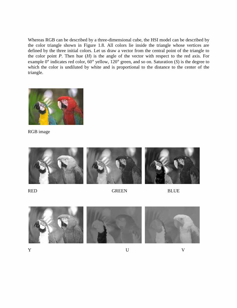
Whereas RGB can be described by a three-dimensional cube, the HSI model can be described bythe color triangle shown in Figure 1.8. All colors lie inside the triangle whose vertices aredefined by the three initial colors. Let us draw a vector from the central point of the triangle tothe color point P. Then hue (H) is the angle of the vector with respect to the red axis. Forexample 0 indicates red color, 60 yellow, 120 green, and so on. Saturation (S) is the degree towhich the color is undiluted by white and is proportional to the distance to the center of thetriangle.
RGB image
RED GREEN BLUE
Y U V
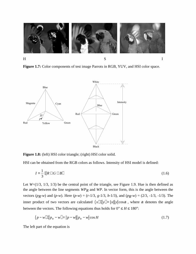
H S I
Figure 1.7: Color components of test image Parrots in RGB, YUV, and HSI color space.
Red Green
Blue
CyanMagenta
YellowPH Red Green
Blue
White
Black
Intensity
Figure 1.8: (left) HSI color triangle; (right) HSI color solid.
HSI can be obtained from the RGB colors as follows. Intensity of HSI model is defined:
I R G B 1
3(1.6)
Let W=(1/3, 1/3, 1/3) be the central point of the triangle, see Figure 1.9. Hue is then defined asthe angle between the line segments WPR and WP. In vector form, this is the angle between the
vectors (pR-w) and (p-w). Here (p-w) = (r-1/3, g-1/3, b-1/3), and (pR-w) = (2/3, -1/3, -1/3). The
inner product of two vectors are calculated x y x y cos , where denotes the angle
between the vectors. The following equations thus holds for 0 H 180:
p w p w p w p w HR R cos (1.7)
The left part of the equation is
p w p w r g b
r g b
R G B
R G B
R
2
3
1
3
1
3
1
3
1
3
1
3
2
32
3
(1.8)
PR
PG
PB
W
(1,0,1)
(0,0,1)
(1,0,0)
Blue
Green
Red
PT
P
P'
Q
PR
PG
PB
W
(0,0,1)
(1,0,1)
(1,0,0)
Blue
Green
Red
1/3
1/3
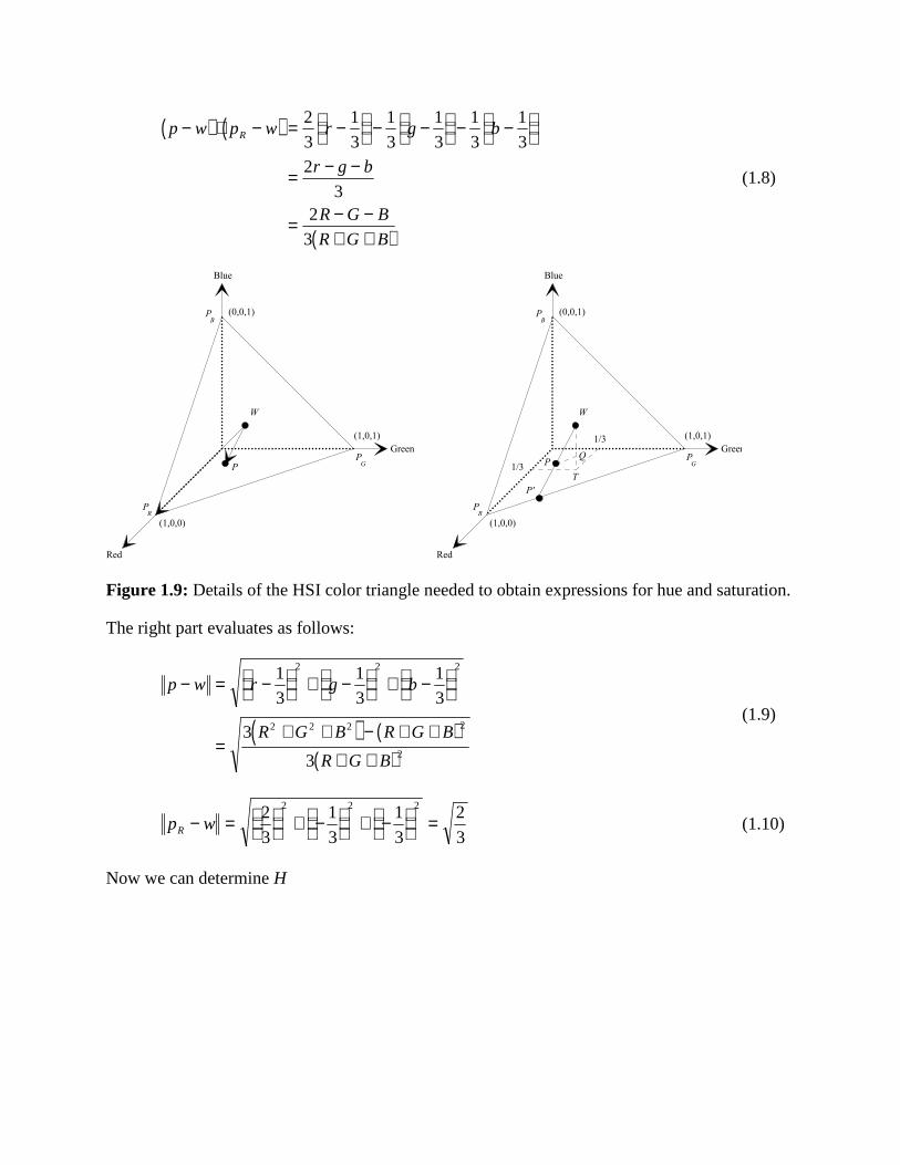
Figure 1.9: Details of the HSI color triangle needed to obtain expressions for hue and saturation.
The right part evaluates as follows:
p w r g b
R G B R G B
R G B
1
3
1
3
1
3
3
3
2 2 2
2 2 2 2
2
(1.9)
p wR
2
3
1
3
1
3
2
3
2 2 2
(1.10)
Now we can determine H
Hp w p w
p w p w
R G B
R B G
R G B
R G B R G B
R G R B
R G R B G B
R
R
cos
cos
cos
1
12
2
1
2
2
3
9
6 2
12
12
(1.11)
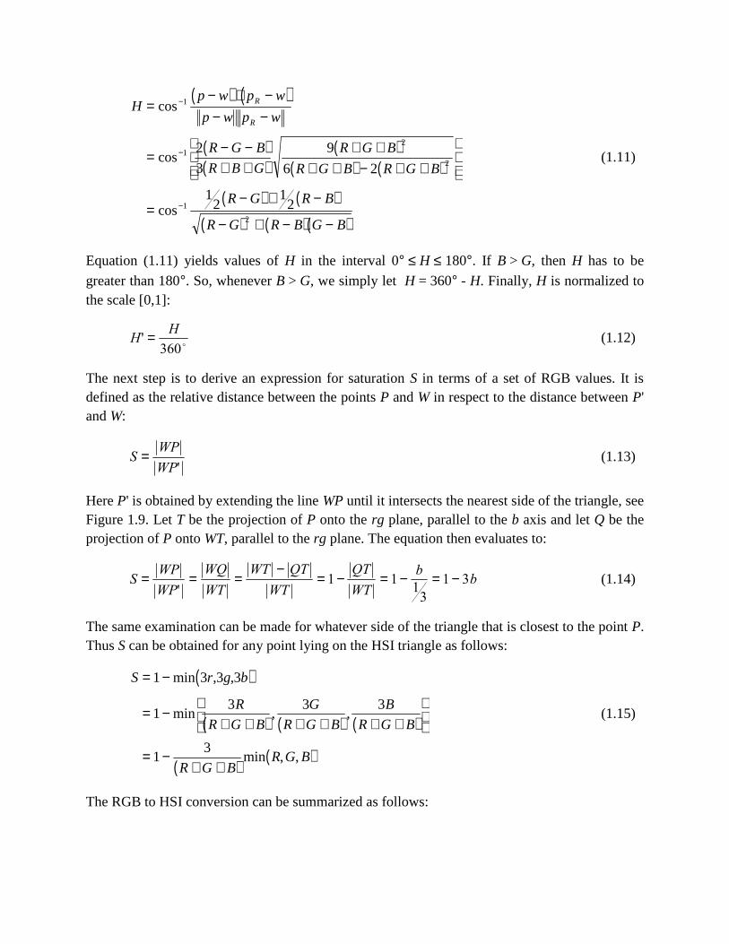
Equation (1.11) yields values of H in the interval 0 H 180. If B > G, then H has to be
greater than 180. So, whenever B > G, we simply let H = 360 - H. Finally, H is normalized tothe scale [0,1]:
H H' 360
(1.12)
The next step is to derive an expression for saturation S in terms of a set of RGB values. It isdefined as the relative distance between the points P and W in respect to the distance between P'and W:
S WPWP
'
(1.13)
Here P' is obtained by extending the line WP until it intersects the nearest side of the triangle, seeFigure 1.9. Let T be the projection of P onto the rg plane, parallel to the b axis and let Q be theprojection of P onto WT, parallel to the rg plane. The equation then evaluates to:
S WPWP
WQWT
WT QTWT
QTWT
b b
'
1 1 13
1 3 (1.14)
The same examination can be made for whatever side of the triangle that is closest to the point P.Thus S can be obtained for any point lying on the HSI triangle as follows:
S r g b
R
R G B
G
R G B
B
R G B
R G BR G B
1 3 3 3
13 3 3
13
min , ,
min , ,
min , ,
(1.15)
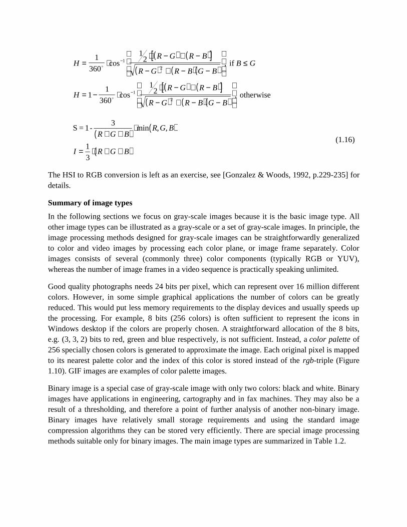
The RGB to HSI conversion can be summarized as follows:
HR G R B
R G R B G BB G
HR G R B
R G R B G B
1
360
12
11
360
12
1
2
1
2
cos
cos ,
, if
otherwise
S = 1-3
R G BR G B
I R G B
min , ,
1
3
(1.16)
The HSI to RGB conversion is left as an exercise, see [Gonzalez & Woods, 1992, p.229-235] fordetails.
Summary of image types
In the following sections we focus on gray-scale images because it is the basic image type. Allother image types can be illustrated as a gray-scale or a set of gray-scale images. In principle, theimage processing methods designed for gray-scale images can be straightforwardly generalizedto color and video images by processing each color plane, or image frame separately. Colorimages consists of several (commonly three) color components (typically RGB or YUV),whereas the number of image frames in a video sequence is practically speaking unlimited.
Good quality photographs needs 24 bits per pixel, which can represent over 16 million differentcolors. However, in some simple graphical applications the number of colors can be greatlyreduced. This would put less memory requirements to the display devices and usually speeds upthe processing. For example, 8 bits (256 colors) is often sufficient to represent the icons inWindows desktop if the colors are properly chosen. A straightforward allocation of the 8 bits,e.g. (3, 3, 2) bits to red, green and blue respectively, is not sufficient. Instead, a color palette of256 specially chosen colors is generated to approximate the image. Each original pixel is mappedto its nearest palette color and the index of this color is stored instead of the rgb-triple (Figure1.10). GIF images are examples of color palette images.
Binary image is a special case of gray-scale image with only two colors: black and white. Binaryimages have applications in engineering, cartography and in fax machines. They may also be aresult of a thresholding, and therefore a point of further analysis of another non-binary image.Binary images have relatively small storage requirements and using the standard imagecompression algorithms they can be stored very efficiently. There are special image processingmethods suitable only for binary images. The main image types are summarized in Table 1.2.

Table 1.2: Summary of image types.
Image type Typicalbpp
No. of
Colors
Common
file formats
Binary image 1 2 JBIG, PCX, GIF,TIFF
Gray-scale 8 256 JPEG, GIF, PNG,TIFF
Color image 24 16.6 106 JPEG, PNG, TIFF
Color palette image 8 256 GIF, PNG
Video image 24 16.6 106 MPEG
42 9855 19
Image
R G B012
97
...
9899
255
64 64 0
Figure 1.10: Look-up table for a color palette image.
SIMULTANEOUS CONTRAST• The simultaneous contrast phenomenon is illustrated below.• The small squares in each image are the same intensity.• Because the different background intensities, the small squares do not appear equally bright.• Perceiving the two squares on different backgrounds as different, even thought they are in factidentical, is called the simultaneous contrast effect.• Psychophysically, we say this effect is caused by the difference in the backgrounds, but what is thephysiological mechanism behind this effect?
LATERAL INHIBITION

• Record signal from nerve fiber of receptor A.• Illumination of receptor A alone causes a large response.• Add illumination to three nearby receptors at B causes the response at A to decrease.• Increasing the illumination of B further decreases A’s response.• Thus, illumination of the neighboring receptors inhibited the firing of receptor A.• This inhibition is called lateral inhibition because it is transmitted laterally, across the retina, in astructure called the lateral plexus.• A neural signal is assumed to be generated by a weighted contribution of many spatially adjacentrods and cones.• Some receptors exert an inhibitory influence on the neural response.• The weighting values are, in effect, the impulse response of the human visual system beyond theretina.MACH BAND EFFECT• Another effect that can be explained by the lateral inhibition.• The Mach band effect is illustrated in the figure below.• The intensity is uniform over the width of each bar.• However, the visual appearance is that each strip is darker at its right side than its left.MACH BAND• The Mach band effect is illustrated in the figure below.• A bright bar appears at position B and a dark bar appears at D.MODULATION TRANSFER FUNCTION (MTF) EXPERIMENT• An observer is shown two sine wave grating transparencies, a reference grating of constant contrastand spatial frequency, and a variable-contrast test grating whose spatial frequency is set at somevalue different from that of the reference.• Contrast is defined as the ratio (max-min)/(max+min) where max and min are the maximum andminimum of the grating intensity, respectively.• The contrast of the test grating is varied until the brightness of the bright and dark regions of thetwo transparencies appear identical.• In this manner it is possible to develop a plot of the MTF of the human visual system.• Note that the response is nearly linear for an exponential sine wave grating.MONOCHROME VISION MODEL• The logarithmic/linear system eye model provides a reasonable prediction of visual response over awide range of intensities.• However, at high spatial frequencies and at very low or very high intensities, observed responsesdepart from responses predicted by the model.LIGHT• Light exhibits some properties that make it appear to consist of particles; at other times, it behaveslike a wave.• Light is electromagnetic energy that radiates from a source of energy (or a source of light) in theform of waves• Visible light is in the 400 nm – 700 nm range of electromagnetic spectrumINTENSITY OF LIGHT• The strength of the radiation from a light source is measured using the unit called the candela, orcandle power. The total energy from the light source, including heat and all electromagneticradiation, is called radiance and is usually expressed in watts.• Luminance is a measure of the light strength that is actually perceived by the human eye. Radianceis a measure of the total output of the source; luminance measures just the portion that is perceived.Brightness is a subjective, psychological measure of perceived intensity.
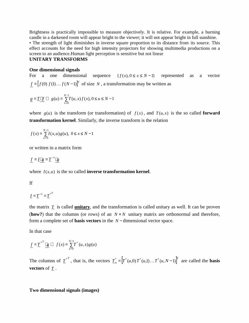
Brightness is practically impossible to measure objectively. It is relative. For example, a burningcandle in a darkened room will appear bright to the viewer; it will not appear bright in full sunshine.• The strength of light diminishes in inverse square proportion to its distance from its source. Thiseffect accounts for the need for high intensity projectors for showing multimedia productions on ascreen to an audience.Human light perception is sensitive but not linearUNITARY TRANSFORMS
One dimensional signalsFor a one dimensional sequence }10),({ Nxxf represented as a vector
TNffff )1()1()0( of size N , a transformation may be written as
10,)(),()(1
0
NuxfxuTugfTg
N
x
where )(ug is the transform (or transformation) of )(xf , and ),( xuT is the so called forward
transformation kernel. Similarly, the inverse transform is the relation
1
010),(),()(
N
uNxuguxIxf
or written in a matrix form
gTgIf 1
where ),( uxI is the so called inverse transformation kernel.
If
TTTI 1
the matrix T is called unitary, and the transformation is called unitary as well. It can be proven
(how?) that the columns (or rows) of an N N unitary matrix are orthonormal and therefore,form a complete set of basis vectors in the N dimensional vector space.
In that case
1
0)(),()(
N
u
TugxuTxfgTf
The columns ofT
T , that is, the vectors Tu NuTuTuTT )1,()1,()0,( are called the basis
vectors of T .
Two dimensional signals (images)
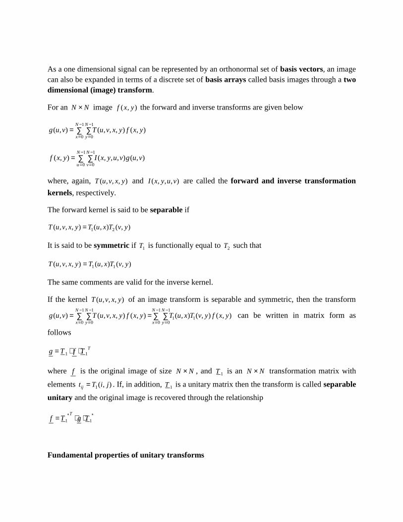
As a one dimensional signal can be represented by an orthonormal set of basis vectors, an imagecan also be expanded in terms of a discrete set of basis arrays called basis images through a twodimensional (image) transform.
For an N N image f x y( , ) the forward and inverse transforms are given below
1
0
1
0),(),,,(),(
N
x
N
yyxfyxvuTvug
1
0
1
0),(),,,(),(
N
u
N
vvugvuyxIyxf
where, again, ),,,( yxvuT and ),,,( vuyxI are called the forward and inverse transformation
kernels, respectively.
The forward kernel is said to be separable if
),(),(),,,( 21 yvTxuTyxvuT
It is said to be symmetric if 1T is functionally equal to 2T such that
),(),(),,,( 11 yvTxuTyxvuT
The same comments are valid for the inverse kernel.
If the kernel ),,,( yxvuT of an image transform is separable and symmetric, then the transform
1
01
1
01
1
0
1
0),(),(),(),(),,,(),(
N
x
N
y
N
x
N
yyxfyvTxuTyxfyxvuTvug can be written in matrix form as
follows
TTfTg 11
where f is the original image of size N N , and 1T is an N N transformation matrix with
elements ),(1 jiTtij . If, in addition, 1T is a unitary matrix then the transform is called separable
unitary and the original image is recovered through the relationship
11 TgTfT
Fundamental properties of unitary transforms

The property of energy preservation
In the unitary transformation
fTg
it is easily proven (try the proof by using the relation T TT 1 ) that
22fg
Thus, a unitary transformation preserves the signal energy. This property is called energypreservation property.
This means that every unitary transformation is simply a rotation of the vector f in the N -
dimensional vector space.
For the 2-D case the energy preservation property is written as
f x y g u vy
N
x
N
v
N
u
N( , ) ( , )
2
0
1
0
1 2
0
1
0
1
The property of energy compactionMost unitary transforms pack a large fraction of the energy of the image into relatively few ofthe transform coefficients. This means that relatively few of the transform coefficients havesignificant values and these are the coefficients that are close to the origin (small indexcoefficients).
This property is very useful for compression purposes. (Why?)
THE TWO DIMENSIONAL FOURIER TRANSFORM
Continuous space and continuous frequency
The Fourier transform is extended to a function f x y( , ) of two variables. If f x y( , ) is continuous
and integrable and F u v( , ) is integrable, the following Fourier transform pair exists:
dxdyeyxfvuF vyuxj )(2),(),(
dudvevuFyxf vyuxj )(22
),()2(
1),(

In general F u v( , ) is a complex-valued function of two real frequency variables u v, and hence, it
can be written as:
),(),(),( vujIvuRvuF
The amplitude spectrum, phase spectrum and power spectrum, respectively, are defined asfollows.
F u v R u v I u v( , ) ( , ) ( , ) 2 2
),(
),(tan),( 1
vuR
vuIvu
P u v F u v R u v I u v( , ) ( , ) ( , ) ( , ) 2 2 2
Discrete space and continuous frequency
For the case of a discrete sequence ),( yxf of infinite duration we can define the 2-D discrete
space Fourier transform pair as follows
x y
vyxujeyxfvuF )(),(),(
dudvevuFyxf vyxuj
u v
)(2
),()2(
1),(
F u v( , ) is again a complex-valued function of two real frequency variables u v, and it is periodic
with a period 2 2 , that is to say F u v F u v F u v( , ) ( , ) ( , ) 2 2
The Fourier transform of f x y( , ) is said to converge uniformly when F u v( , ) is finite and
),(),(limlim1
1
2
221
)( vuFeyxfN
Nx
N
Ny
vyxuj
NN
for all u v, .
When the Fourier transform of f x y( , ) converges uniformly, F u v( , ) is an analytic function and
is infinitely differentiable with respect to u and v .
Discrete space and discrete frequency: The two dimensional Discrete Fourier Transform(2-D DFT)
If f x y( , ) is an NM array, such as that obtained by sampling a continuous function of two
dimensions at dimensions NM and on a rectangular grid, then its two dimensional DiscreteFourier transform (DFT) is the array given by
1
0
1
0
)//(2),(1
),(M
x
N
y
NvyMuxjeyxfMN
vuF
1,,0 Mu , 1,,0 Nv
and the inverse DFT (IDFT) is
f x y F u v e j ux M vy N
v
N
u
M( , ) ( , ) ( / / )
2
0
1
0
1
When images are sampled in a square array, M N and
F u vN
f x y e j ux vy N
y
N
x
N( , ) ( , ) ( )/
1 2
0
1
0
1
f x yN
F u v e j ux vy N
v
N
u
N( , ) ( , ) ( )/
1 2
0
1
0
1
It is straightforward to prove that the two dimensional Discrete Fourier Transform is separable,symmetric and unitary.
Properties of the 2-D DFTMost of them are straightforward extensions of the properties of the 1-D Fourier Transform.Advise any introductory book on Image Processing.
The importance of the phase in 2-D DFT. Image reconstruction from amplitude or phaseonly.
The Fourier transform of a sequence is, in general, complex-valued, and the uniquerepresentation of a sequence in the Fourier transform domain requires both the phase and themagnitude of the Fourier transform. In various contexts it is often desirable to reconstruct asignal from only partial domain information. Consider a 2-D sequence ),( yxf with Fourier
transform ),(),( yxfvuF so that
),(),(},({),(
vuj fevuFyxfvuF
It has been observed that a straightforward signal synthesis from the Fourier transform phase),( vuf alone, often captures most of the intelligibility of the original image ),( yxf (why?). A
straightforward synthesis from the Fourier transform magnitude ),( vuF alone, however, does
not generally capture the original signal’s intelligibility. The above observation is valid for alarge number of signals (or images). To illustrate this, we can synthesise the phase-only signal
),( yxf p and the magnitude-only signal ),( yxfm by
),(1 1),(vuj
pfeyxf

01 ),(),( jm evuFyxf
and observe the two results (Try this exercise in MATLAB).
An experiment which more dramatically illustrates the observation that phase-only signalsynthesis captures more of the signal intelligibility than magnitude-only synthesis, can beperformed as follows.
Consider two images ),( yxf and ),( yxg . From these two images, we synthesise two other
images ),(1 yxf and ),(1 yxg by mixing the amplitudes and phases of the original images as
follows:
),(11 ),(),(
vuj fevuGyxf
),(11 ),(),(
vuj gevuFyxg
In this experiment ),(1 yxf captures the intelligibility of ),( yxf , while ),(1 yxg captures the
intelligibility of ),( yxg (Try this exercise in MATLAB).
THE DISCRETE COSINE TRANSFORM (DCT)One dimensional signals
This is a transform that is similar to the Fourier transform in the sense that the new independentvariable represents again frequency. The DCT is defined below.
1
0 2)12(
cos)()()(N
x N
uxxfuauC
, 1,,1,0 Nu
with )(ua a parameter that is defined below.
1,,1/2
0/1
)(
NuN
uN
ua
The inverse DCT (IDCT) is defined below.
1
0 2)12(
cos)()()(N
u N
uxuCuaxf
Two dimensional signals (images)
For 2-D signals it is defined as

N
vy
N
uxyxfvauavuC
N
x
N
y 2)12(
cos2
)12(cos),()()(),(
1
0
1
0
N
vy
N
uxvuCvauayxf
N
u
N
v 2)12(
cos2
)12(cos),()()(),(
1
0
1
0
)(ua is defined as above and 1,,1,0, Nvu
Properties of the DCT transform
The DCT is a real transform. This property makes it attractive in comparison to the Fouriertransform.
The DCT has excellent energy compaction properties. For that reason it is widely used inimage compression standards (as for example JPEG standards).
There are fast algorithms to compute the DCT, similar to the FFT for computing the DFT. KARHUNEN-LOEVE (KLT) or HOTELLING TRANSFORMThe Karhunen-Loeve Transform or KLT was originally introduced as a series expansion forcontinuous random processes by Karhunen and Loeve. For discrete signals Hotelling first studiedwhat was called a method of principal components, which is the discrete equivalent of the KLseries expansion. Consequently, the KL transform is also called the Hotelling transform or themethod of principal components. The term KLT is the most widely used.
The case of many realisations of a signal or image (Gonzalez/Woods)The concepts of eigenvalue and eigevector are necessary to understand the KL transform.
If C is a matrix of dimension nn , then a scalar is called an eigenvalue of C if there is a
nonzero vector e in nR such that
eeC
The vector e is called an eigenvector of the matrix C corresponding to the eigenvalue .
(If you have difficulties with the above concepts consult any elementary linear algebrabook.)
Consider a population of random vectors of the form
nx
x
x
x2
1
The mean vector of the population is defined as
xEm x
The operator E refers to the expected value of the population calculated theoretically using theprobability density functions (pdf) of the elements ix and the joint probability density functions
between the elements ix and jx .
The covariance matrix of the population is defined as
Txxx mxmxEC ))((
Because x is n -dimensional, xC and Txx mxmx ))(( are matrices of order nn . The element
iic of xC is the variance of ix , and the element ijc of xC is the covariance between the elements
ix and jx . If the elements ix and jx are uncorrelated, their covariance is zero and, therefore,
0 jiij cc .
For M vectors from a random population, where M is large enough, the mean vector andcovariance matrix can be approximately calculated from the vectors by using the followingrelationships where all the expected values are approximated by summations
M
kkx x
Mm
1
1
Txx
Tk
M
kkx mmxx
MC
1
1
Very easily it can be seen that xC is real and symmetric. In that case a set of n orthonormal (at
this point you are familiar with that term) eigenvectors always exists. Let ie and i ,
ni ,,2,1 , be this set of eigenvectors and corresponding eigenvalues of xC , arranged in
descending order so that 1 ii for 1,,2,1 ni . Let A be a matrix whose rows are formed
from the eigenvectors of xC , ordered so that the first row of A is the eigenvector corresponding
to the largest eigenvalue, and the last row the eigenvector corresponding to the smallesteigenvalue.
Suppose that A is a transformation matrix that maps the vectors sx ' into vectors sy ' by using
the following transformation
)( xmxAy
The above transform is called the Karhunen-Loeve or Hotelling transform. The mean of the y
vectors resulting from the above transformation is zero (try to prove that)
0ym
the covariance matrix is (try to prove that)
Txy ACAC
and yC is a diagonal matrix whose elements along the main diagonal are the eigenvalues of xC
(try to prove that)
n
yC
0
0
2
1
The off-diagonal elements of the covariance matrix are 0 , so the elements of the y vectors are
uncorrelated.
Lets try to reconstruct any of the original vectors x from its corresponding y . Because the rows
of A are orthonormal vectors (why?), then TAA 1 , and any vector x can by recovered from
its corresponding vector y by using the relation
xT myAx
Suppose that instead of using all the eigenvectors of xC we form matrix KA from the K
eigenvectors corresponding to the K largest eigenvalues, yielding a transformation matrix oforder nK . The y vectors would then be K dimensional, and the reconstruction of any of the
original vectors would be approximated by the following relationship
xTK myAx ˆ
The mean square error between the perfect reconstruction x and the approximate reconstruction
x̂ is given by the expression
n
Kjj
K
jj
n
jjmse
111 .
By using KA instead of A for the KL transform we achieve compression of the available data.
The case of one realisation of a signal or imageThe derivation of the KLT for the case of one image realisation assumes that the twodimensional signal (image) is ergodic. This assumption allows us to calculate the statistics of the
image using only one realisation. Usually we divide the image into blocks and we apply the KLTin each block. This is reasonable because the 2-D field is likely to be ergodic within a smallblock since the nature of the signal changes within the whole image. Let’s suppose that f is a
vector obtained by lexicographic ordering of the pixels ),( yxf within a block of size MM
(placing the rows of the block sequentially).
The mean vector of the random field inside the block is a scalar that is estimated by theapproximate relationship
2
12 )(
1 M
kf kf
Mm
and the covariance matrix of the 2-D random field inside the block is fC where
2
12 )()(
1 2
f
M
kii mkfkf
Mc
and
2
12 )()(
1 2
f
M
kjiij mjikfkf
Mcc
After knowing how to calculate the matrix fC , the KLT for the case of a single realisation is the
same as described above.
Properties of the Karhunen-Loeve transform
Despite its favourable theoretical properties, the KLT is not used in practice for the followingreasons. Its basis functions depend on the covariance matrix of the image, and hence they have to
recomputed and transmitted for every image.
Perfect decorrelation is not possible, since images can rarely be modelled as realisations ofergodic fields.
There are no fast computational algorithms for its implementation.
Singular Value Decomposition (SVD)
• Given any mn matrix A, algorithm to find matrices U, V, and W such that
A = U W VT
U is mn and orthonormal
W is nn and diagonal
V is nn and orthonormal
UNIT II
IMAGE ENHANCEMENT
Spatial domain methodsSuppose we have a digital image which can be represented by a two dimensional random field
),( yxf . An image processing operator in the spatial domain may be expressed as a mathematical
function T applied to the image ),( yxf to produce a new image ),(),( yxfTyxg as follows.
),(),( yxfTyxg The operator T applied on ),( yxf may be defined over:
(i) A single pixel ),( yx . In this case T is a grey level transformation (or mapping) function.
(ii) Some neighbourhood of ),( yx .
(iii) T may operate to a set of input images instead of a single image.
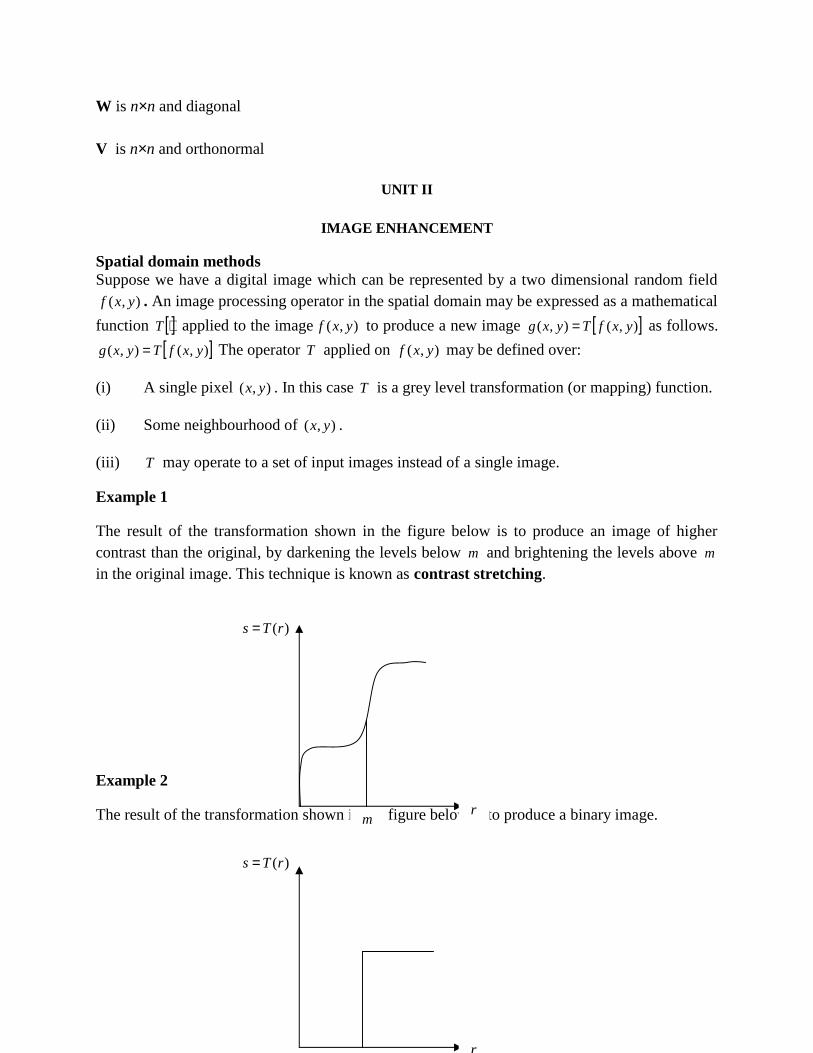
Example 1
The result of the transformation shown in the figure below is to produce an image of highercontrast than the original, by darkening the levels below m and brightening the levels above m
in the original image. This technique is known as contrast stretching.
Example 2
The result of the transformation shown in the figure below is to produce a binary image.m
)(rTs
r
)(rTs
r
1.2 Frequency domain methodsLet ),( yxg be a desired image formed by the convolution of an image ),( yxf and a linear,
position invariant operator ),( yxh , that is: ),(),(),( yxfyxhyxg
The following frequency relationship holds:),(),(),( vuFvuHvuG
We can select ),( vuH so that the desired image
),(),(),( 1 vuFvuHyxg
exhibits some highlighted features of ),( yxf . For instance, edges in ),( yxf can be accentuated
by using a function ),( vuH that emphasises the high frequency components of ),( vuF .
Spatial domain: Enhancement by point processingWe are dealing now with image processing methods that are based only on te intensity of singlepixels.Intensity transformationsImage Negatives
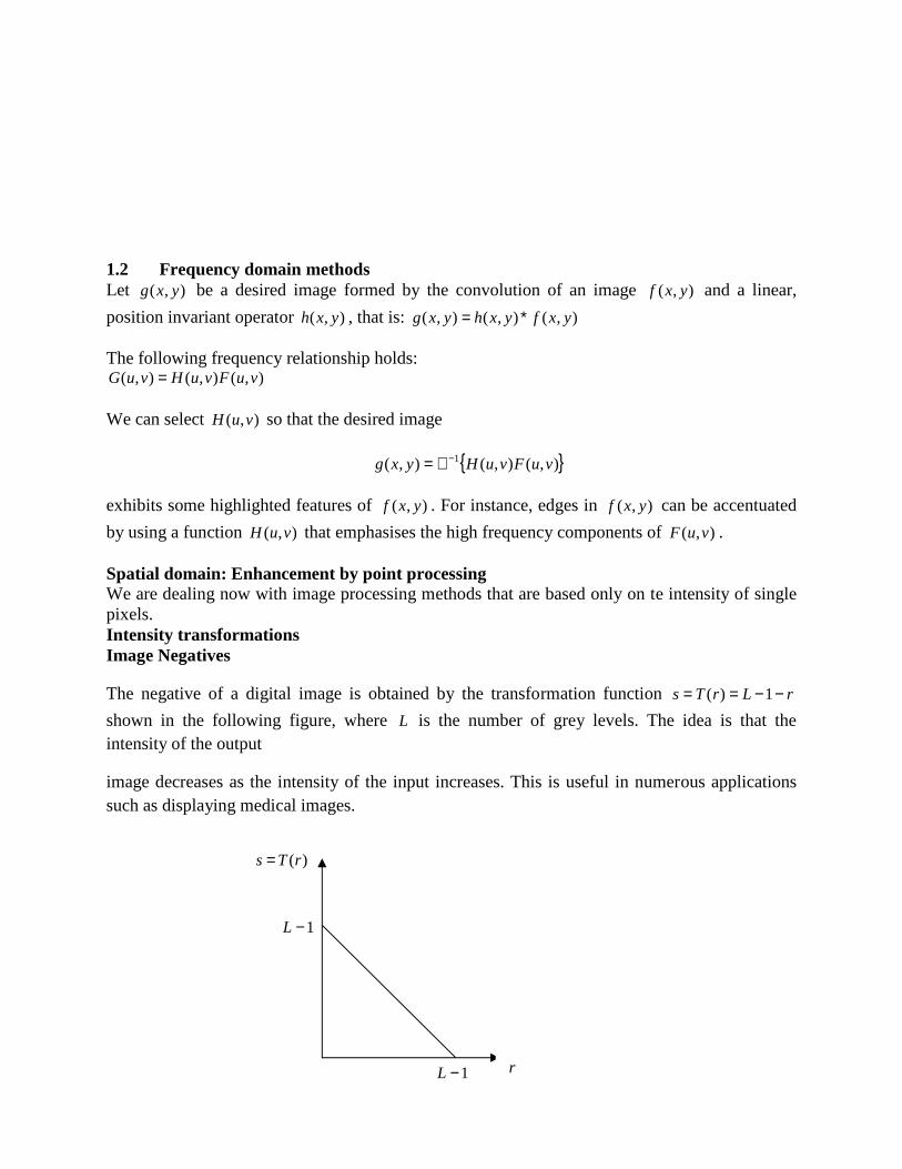
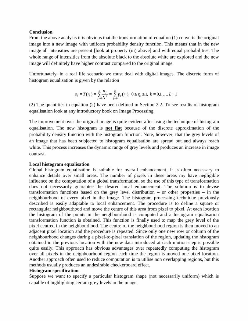
The negative of a digital image is obtained by the transformation function rLrTs 1)(
shown in the following figure, where L is the number of grey levels. The idea is that theintensity of the output
image decreases as the intensity of the input increases. This is useful in numerous applicationssuch as displaying medical images.
1L
1L
)(rTs
r

Contrast StretchingLow contrast images occur often due to poor or non uniform lighting conditions, or due tononlinearity, or small dynamic range of the imaging sensor. In the figure of Example 1 aboveyou have seen a typical contrast stretching transformation.
Histogram processing. Definition of the histogram of an image.By processing (modifying) the histogram of an image we can create a new image with specificdesired properties. Suppose we have a digital image of size NN with grey levels in the range
]1,0[ L . The histogram of the image is defined as the following discrete function:
2)(
N
nrp kk
where
kr is the thk grey level, 1,,1,0 Lk
kn is the number of pixels in the image with grey level kr
2N is the total number of pixels in the image
The histogram represents the frequency of occurrence of the various grey levels in the image. Aplot of this function for all values of k provides a global description of the appearance of theimage.
Global histogram equalisationIn this section we will assume that the image to be processed has a continuous intensity that lieswithin the interval ]1,0[ L . Suppose we divide the image intensity with its maximum value
1L . Let the variable r represent the new grey levels (image intensity) in the image, where now10 r and let )(rpr denote the probability density function (pdf) of the variable r . We now
apply the following transformation function to the intensity
r
r dwwprTs0
)()( , 10 r
(1) By observing the transformation of equation (1) we immediately see that it possesses thefollowing properties:
(i) 10 s .
(ii) )()( 1212 rTrTrr , i.e., the function )(rT is increase ng with r .
(iii) 0)()0(0
0
dwwpTs r and 1)()1(1
0
dwwpTs r . Moreover, if the original image has
intensities only within a certain range ],[ maxmin rr then 0)()(min
0min
r
r dwwprTs and
1)()(max
0max
r
r dwwprTs since maxmin and,0)( rrrrrpr . Therefore, the new intensity
s takes always all values within the available range [0 1].
Suppose that )(rPr , )(sPs are the probability distribution functions (PDF’s) of the variables r
and s respectively.
Let us assume that the original intensity lies within the values r and drr with dr a smallquantity. dr can be assumed small enough so as to be able to consider the function )(wpr
constant within the interval ],[ drrr and equal to )(rpr . Therefore,
drrpdwrpdwwpdrrrP r
drr
rr
drr
rrr )()()(],[
.
Now suppose that )(rTs and )(1 drrTs . The quantity dr can be assumed small enough so
as to be able to consider that dsss 1 with ds small enough so as to be able to consider the
function )(wps constant within the interval ],[ dsss and equal to )(sps . Therefore,
dsspdwspdwwpdsssP s
dss
ss
dss
sss )()()(],[
Since )(rTs , )( drrTdss and the function of equation (1) is increasing with r , all and
only the values within the interval ],[ drrr will be mapped within the interval ],[ dsss .
Therefore,
],[],[ dsssPdrrrP sr)(
)(
1
1
)()()()(sTr
rss
sTr
r ds
drrpspdsspdrrp
From equation (1) we see that
)(rpdr
dsr
and hence,
10,1)(
1)()(
)(1
srp
rpspsTrr
rs
ConclusionFrom the above analysis it is obvious that the transformation of equation (1) converts the originalimage into a new image with uniform probability density function. This means that in the newimage all intensities are present [look at property (iii) above] and with equal probabilities. Thewhole range of intensities from the absolute black to the absolute white are explored and the newimage will definitely have higher contrast compared to the original image.
Unfortunately, in a real life scenario we must deal with digital images. The discrete form ofhistogram equalisation is given by the relation
k
jkjr
k
j
jkk Lkrrp
N
nrTs
002 1,,1,0,10),()(
(2) The quantities in equation (2) have been defined in Section 2.2. To see results of histogramequalisation look at any introductory book on Image Processing.
The improvement over the original image is quite evident after using the technique of histogramequalisation. The new histogram is not flat because of the discrete approximation of theprobability density function with the histogram function. Note, however, that the grey levels ofan image that has been subjected to histogram equalisation are spread out and always reachwhite. This process increases the dynamic range of grey levels and produces an increase in imagecontrast.
Local histogram equalisationGlobal histogram equalisation is suitable for overall enhancement. It is often necessary toenhance details over small areas. The number of pixels in these areas my have negligibleinfluence on the computation of a global transformation, so the use of this type of transformationdoes not necessarily guarantee the desired local enhancement. The solution is to devisetransformation functions based on the grey level distribution – or other properties – in theneighbourhood of every pixel in the image. The histogram processing technique previouslydescribed is easily adaptable to local enhancement. The procedure is to define a square orrectangular neighbourhood and move the centre of this area from pixel to pixel. At each locationthe histogram of the points in the neighbourhood is computed and a histogram equalisationtransformation function is obtained. This function is finally used to map the grey level of thepixel centred in the neighbourhood. The centre of the neighbourhood region is then moved to anadjacent pixel location and the procedure is repeated. Since only one new row or column of theneighbourhood changes during a pixel-to-pixel translation of the region, updating the histogramobtained in the previous location with the new data introduced at each motion step is possiblequite easily. This approach has obvious advantages over repeatedly computing the histogramover all pixels in the neighbourhood region each time the region is moved one pixel location.Another approach often used to reduce computation is to utilise non overlapping regions, but thismethods usually produces an undesirable checkerboard effect.Histogram specificationSuppose we want to specify a particular histogram shape (not necessarily uniform) which iscapable of highlighting certain grey levels in the image.
Let us suppose that:
)(rpr is the original probability density function
)(zpz is the desired probability density function
Suppose that histogram equalisation is first applied on the original image r
r
r dwwprTs0
)()(
Suppose that the desired image z is available and histogram equalisation is applied as well
z
z dwwpzGv0
)()(
)(sps and )(vpv are both uniform densities and they can be considered as identical. Note that the
final result of histogram equalisation is independent of the density inside the integral. So in
equation z
z dwwpzGv0
)()( we can use the symbol s instead of v .
The inverse process )(1 sGz will have the desired probability density function. Therefore, the
process of histogram specification can be summarised in the following steps.
(i) We take the original image and equalise its intensity using the relation
r
r dwwprTs0
)()( .
(ii) From the given probability density function )(zpz we specify the probability distribution
function )(zG .
(iii) We apply the inverse transformation function )()( 11 rTGsGz
Spatial domain: Enhancement in the case of many realisations of an image of interestavailable
Image averagingSuppose that we have an image ),( yxf of size NM pixels corrupted by noise ),( yxn , so we
obtain a noisy image as follows.
),(),(),( yxnyxfyxg
For the noise process ),( yxn the following assumptions are made.
(i) The noise process ),( yxn is ergodic.
(ii) It is zero mean, i.e.,
1
0
1
00),(
1),(
M
x
N
yyxn
MNyxnE
(ii) It is white, i.e., the autocorrelation function of the noise process defined as
kM
x
lN
ylykxnyxn
lNkMlykxnyxnElkR
1
0
1
0),(),(
))((1
)},(),({],[ is zero, apart
for the pair ]0,0[],[ lk .
Therefore, ),(),(),())((
1,
1
0
1
0
2),( lklykxnyxn
lNkMlkR
kM
x
lN
yyxn
where 2
),( yxn
is the variance of noise.
Suppose now that we have L different noisy realisations of the same image ),( yxf as
),(),(),( yxnyxfyxg ii , Li ,,1,0 . Each noise process ),( yxni satisfies the properties (i)-
(iii) given above. Moreover, 22),( yxni
. We form the image ),( yxg by averaging these L noisy
images as follows:
L
ii
L
ii
L
ii yxn
Lyxfyxnyxf
Lyxg
Lyxg
111),(
1),()),(),((
1),(
1),(
Therefore, the new image is again a noisy realisation of the original image ),( yxf with noise
L
ii yxn
Lyxn
1),(
1),( .
The mean value of the noise ),( yxn is found below.
0)},({1
)},(1
{)},({11
L
ii
L
ii yxnE
Lyxn
LEyxnE
The variance of the noise ),( yxn is now found below.
2
1
22
1 12
1
22
1 12
1
22
2
12
2
1
22),(
10
1
)},(),({1
)},({1
))},(),(({(1
)}),({(1
),(1
),(1
)},({
LL
yxnyxnEL
yxnEL
yxnyxnEL
yxnEL
yxnEL
yxnL
EyxnE
L
i
ji
ji
L
i
L
j
L
iiji
ji
L
i
L
j
L
ii
L
ii
L
iiyxn
Therefore, we have shown that image averaging produces an image ),( yxg , corrupted by noise
with variance less than the variance of the noise of the original noisy images. Note that if L
we have 02),( yxn , the resulting noise is negligible.
Spatial domain: Enhancement in the case of a single image
Spatial masks
Many image enhancement techniques are based on spatial operations performed on localneighbourhoods of input pixels.
The image is usually convolved with a finite impulse response filter called spatial mask. The useof spatial masks on a digital image is called spatial filtering.
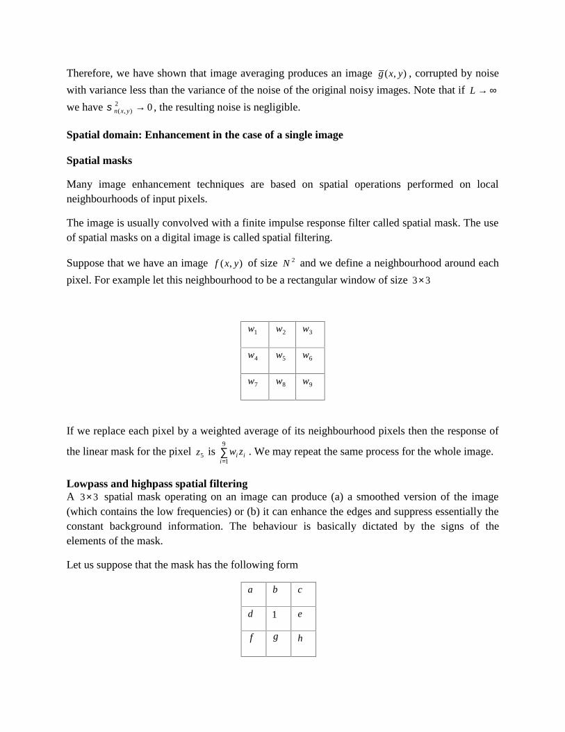
Suppose that we have an image ),( yxf of size 2N and we define a neighbourhood around each
pixel. For example let this neighbourhood to be a rectangular window of size 33
1w 2w 3w
4w 5w 6w
7w 8w 9w
If we replace each pixel by a weighted average of its neighbourhood pixels then the response of
the linear mask for the pixel 5z is
9
1iii zw . We may repeat the same process for the whole image.
Lowpass and highpass spatial filteringA 33 spatial mask operating on an image can produce (a) a smoothed version of the image(which contains the low frequencies) or (b) it can enhance the edges and suppress essentially theconstant background information. The behaviour is basically dictated by the signs of theelements of the mask.
Let us suppose that the mask has the following form
a b c
d 1 e
f g h

To be able to estimate the effects of the above mask with relation to the sign of the coefficientshgfedcba ,,,,,,, , we will consider the equivalent one dimensional mask
d 1 e
Let us suppose that the above mask is applied to a signal )(nx . The output of this operation will
be a signal )(ny as )()()()()1()()1()( 1 zezXzXzXdzzYnexnxndxny
)()1()( 1 zXezdzzY ezdzzHzX
zY 1)(
)(
)( 1 . This is the transfer function of a system
that produces the above input-output relationship. In the frequency domain we have
)exp(1)exp()( jejdeH j .
The values of this transfer function at frequencies 0 and are:
edeH j
1)(0
edeH j
1)(
If a lowpass filtering (smoothing) effect is required then the following condition must hold
0)()(0
edeHeH jj
If a highpass filtering effect is required then
0)()(0
edeHeH jj
The most popular masks for lowpass filtering are masks with all their coefficients positive andfor highpass filtering, masks where the central pixel is positive and the surrounding pixels arenegative or the other way round.
Popular techniques for lowpass spatial filteringUniform filtering
The most popular masks for lowpass filtering are masks with all their coefficients positive andequal to each other as for example the mask shown below. Moreover, they sum up to 1 in orderto maintain the mean of the image.
91
11
111
1

Gaussian filtering
The two dimensional Gaussian mask has values that attempts to approximate the continuousfunction
2
22
22
1),(
yx
eyxG
In theory, the Gaussian distribution is non-zero everywhere, which would require an infinitelylarge convolution kernel, but in practice it is effectively zero more than about three standarddeviations from the mean, and so we can truncate the kernel at this point. The following shows asuitable integer-valued convolution kernel that approximates a Gaussian with a of 1.0.
Median filtering
The median m of a set of values is the value that possesses the property that half the values inthe set are less than m and half are greater than m . Median filtering is the operation that replaceseach pixel by the median of the grey level in the neighbourhood of that pixel.
Median filters are non linear filters because for two sequences )(nx and )(ny
)(median)(median)()(median nynxnynx
Median filters are useful for removing isolated lines or points (pixels) while preserving spatialresolutions. They perform very well on images containing binary (salt and pepper) noise butperform poorly when the noise is Gaussian. Their performance is also poor when the number ofnoise pixels in the window is greater than or half the number of pixels in the window (why?)
2731
264
741
7 26 41
16
26
16
4
4 16 26 16
1 4 7 4
7
4
1
4
1
Isolatedpoint
Median filtering
0
00
0
0
0
0
0
0
0
10
0
0
0
0
0
0

Directional smoothingTo protect the edges from blurring while smoothing, a directional averaging filter can be useful.Spatial averages ):,( yxg are calculated in several selected directions (for example could be
horizontal, vertical, main diagonals)
),(
),(1
):,(lk W
lykxfN
yxg
and a direction is found such that ):,(),( yxgyxf is minimum. (Note that W is the
neighbourhood along the direction and N is the number of pixels within this neighbourhood).
Then by replacing ):,( with):,( yxgyxg we get the desired result.
High Boost FilteringA high pass filtered image may be computed as the difference between the original image and alowpass filtered version of that image as follows:
(Highpass part of image)=(Original)-(Lowpass part of image)
Multiplying the original image by an amplification factor denoted by A , yields the so called highboost filter:
(Highboost image)= )(A (Original)-(Lowpass)= )1( A (Original)+(Original)-(Lowpass)
= )1( A (Original)+(Highpass)
The general process of subtracting a blurred image from an original as given in the first line iscalled unsharp masking. A possible mask that implements the above procedure could be the oneillustrated below.
91
-1
-1-1
-1
-1
-1
-1
-1
-1
0
A0
0
0
0
0
0
0
91
19 A-1-1
-1-1-1
-1 -1 -1
The high-boost filtered image looks more like the original with a degree of edge enhancement,
depending on the value of A .
Popular techniques for highpass spatial filtering. Edge detection using derivative filtersAbout two dimensional high pass spatial filters
An edge is the boundary between two regions with relatively distinct grey level properties. Theidea underlying most edge detection techniques is the computation of a local derivative operator.The magnitude of the first derivative calculated within a neighbourhood around the pixel ofinterest, can be used to detect the presence of an edge in an image.
The gradient of an image ),( yxf at location ),( yx is a vector that consists of the partial
derivatives of ),( yxf as follows.
y
yxf
x
yxf
yxf),(
),(
),(
The magnitude of this vector, generally referred to simply as the gradient f is
2/122),().(
)),((mag),(
y
yxf
x
yxfyxfyxf
Common practice is to approximate the gradient with absolute values which is simpler toimplement as follows.
y
yxf
x
yxfyxf
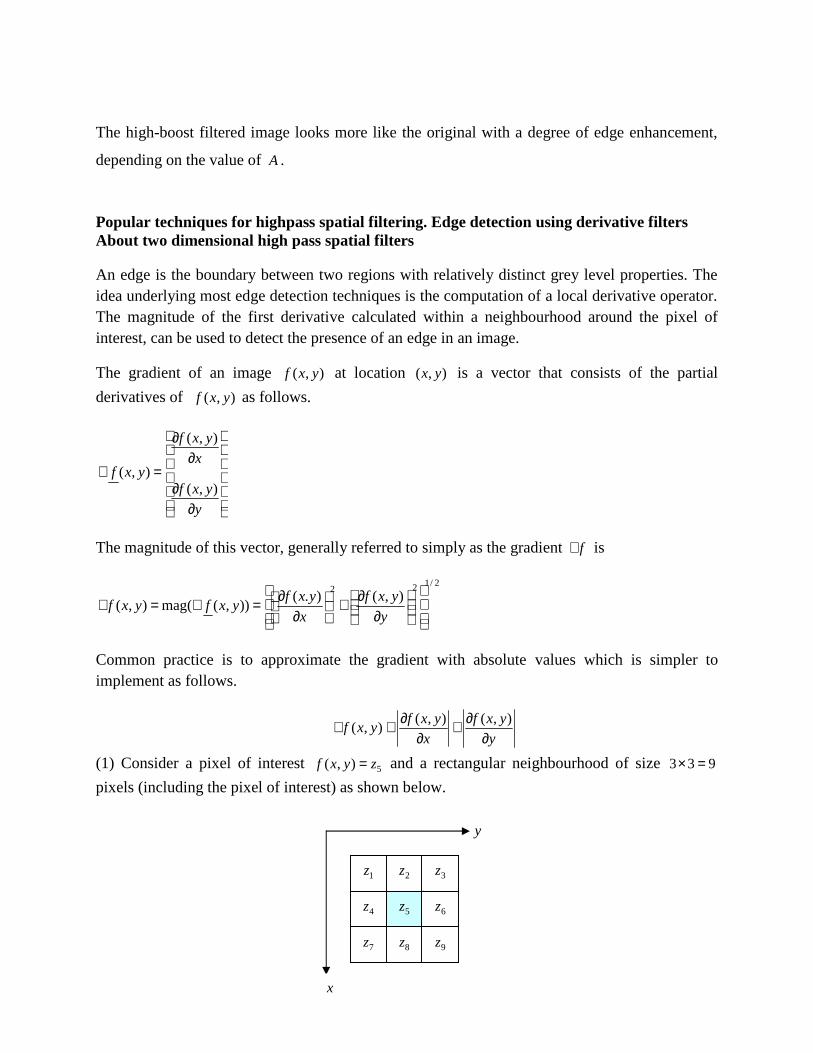
),(),(),(
(1) Consider a pixel of interest 5),( zyxf and a rectangular neighbourhood of size 933
pixels (including the pixel of interest) as shown below.
7z 8z
1z 2z 3z
4z 5z 6z
9z
y
x
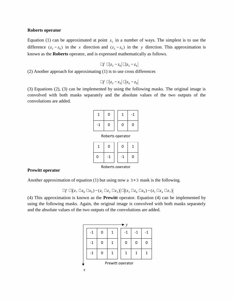
Roberts operator
Equation (1) can be approximated at point 5z in a number of ways. The simplest is to use the
difference )( 85 zz in the x direction and )( 65 zz in the y direction. This approximation is
known as the Roberts operator, and is expressed mathematically as follows.
6585 zzzzf
(2) Another approach for approximating (1) is to use cross differences
8695 zzzzf
(3) Equations (2), (3) can be implemented by using the following masks. The original image isconvolved with both masks separately and the absolute values of the two outputs of theconvolutions are added.
Prewitt operator
Another approximation of equation (1) but using now a 33 mask is the following.
)()()()( 741963321987 zzzzzzzzzzzzf
(4) This approximation is known as the Prewitt operator. Equation (4) can be implemented byusing the following masks. Again, the original image is convolved with both masks separatelyand the absolute values of the two outputs of the convolutions are added.
Roberts operator
0 1
-1 0
1 0
0 -1
1 0
-1 0
1 -1
0 0
Roberts operator
y
x
Prewitt operator
-1
00
1
-1
1
0
-1
1
-1
0-1
0
0
1
1
1
-1
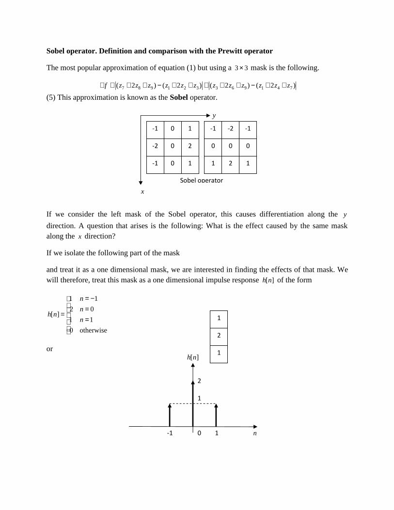
Sobel operator. Definition and comparison with the Prewitt operator
The most popular approximation of equation (1) but using a 33 mask is the following.
)2()2()2()2( 741963321987 zzzzzzzzzzzzf
(5) This approximation is known as the Sobel operator.
If we consider the left mask of the Sobel operator, this causes differentiation along the y
direction. A question that arises is the following: What is the effect caused by the same maskalong the x direction?
If we isolate the following part of the mask
and treat it as a one dimensional mask, we are interested in finding the effects of that mask. Wewill therefore, treat this mask as a one dimensional impulse response ][nh of the form
otherwise0
11
02
11
][n
n
n
nh
or
y
x
Sobel operator
-1
00
2
-2
1
0
-1
1
-1
0-2
0
0
1
2
1
-1
1
2
1
][nh
2
1
-1 10 n
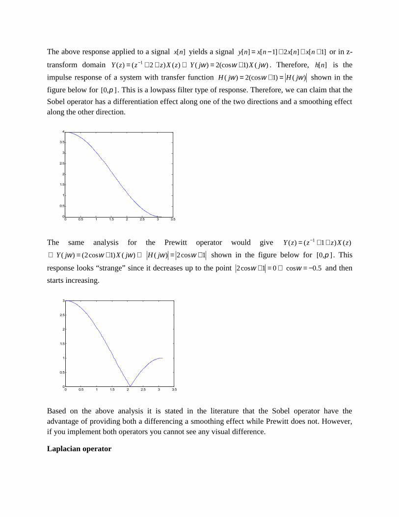
The above response applied to a signal ][nx yields a signal ]1[][2]1[][ nxnxnxny or in z-
transform domain )()1(cos2)()()2()( 1 jXjYzXzzzY . Therefore, ][nh is the
impulse response of a system with transfer function )()1(cos2)( jHjH shown in the
figure below for ],0[ . This is a lowpass filter type of response. Therefore, we can claim that the
Sobel operator has a differentiation effect along one of the two directions and a smoothing effectalong the other direction.
The same analysis for the Prewitt operator would give )()1()( 1 zXzzzY
)()1cos2()( jXjY 1cos2)( jH shown in the figure below for ],0[ . This
response looks “strange” since it decreases up to the point 5.0cos01cos2 and then
starts increasing.
Based on the above analysis it is stated in the literature that the Sobel operator have theadvantage of providing both a differencing a smoothing effect while Prewitt does not. However,if you implement both operators you cannot see any visual difference.
Laplacian operator
0 0.5 1 1.5 2 2.5 3 3.50
0.5
1
1.5
2
2.5
3
3.5
4
0 0.5 1 1.5 2 2.5 3 3.50
0.5
1
1.5
2
2.5
3

The Laplacian of a 2-D function ),( yxf is a second order derivative defined as
2
2
2
22 ),(),(
),(y
yxf
x
yxfyxf
In practice it can be also implemented using a 3x3 mask as follows (why?)
)(4 864252 zzzzzf
The main disadvantage of the Laplacian operator is that it produces double edges.
UNIT III
IMAGE RESTORATION
PreliminariesWhat is image restoration?Image Restoration refers to a class of methods that aim to remove or reduce the degradations that haveoccurred while the digital image was being obtained. All natural images when displayed have gonethrough some sort of degradation:
during display mode
during acquisition mode, or
during processing mode
The degradations may be due to
sensor noise
blur due to camera misfocus
relative object-camera motion
random atmospheric turbulence
others
In most of the existing image restoration methods we assume that the degradation process can bedescribed using a mathematical model.
How well can we do?Depends on how much we know about
the original image
the degradations

(how accurate our models are)
Image restoration and image enhancement difference Image restoration differs from image enhancement in that the latter is concerned more
with accentuation or extraction of image features rather than restoration of degradations.
Image restoration problems can be quantified precisely, whereas enhancement criteria aredifficult to represent mathematically.
Image observation models
Typical parts of an imaging system: image formation system, a detector and a recorder. Ageneral model for such a system could be:
),(),(),( jinjiwrjiy
jdidjifjijihjifHjiw ),(),,,(),(),(
),(),()],([),( 21 jinjinjiwrgjin
where ),( jiy is the degraded image, ),( jif is the original image and ),,,( jijih is an operator
that represents the degradation process, for example a blurring process. Functions g and r
are generally nonlinear, and represent the characteristics of detector/recording mechanisms.),( jin is the additive noise, which has an image-dependent random component
),()],([ 1 jinjifHrg and an image-independent random component ),(2 jin .
Detector and recorder models
The response of image detectors and recorders in general is nonlinear. An example is theresponse of image scanners
),(),( jiwjir
where and are device-dependent constants and ),( jiw is the input blurred image.
For photofilms
010 ),(log),( rjiwjir
where is called the gamma of the film, ),( jiw is the incident light intensity and ),( jir is called
the optical density. A film is called positive if it has negative .
Noise models
The general noise model
),(),()],([),( 21 jinjinjiwrgjin
is applicable in many situations. Example, in photoelectronic systems we may have xxg )( .
Therefore,
),(),(),(),( 21 jinjinjiwjin
where 1n and 2n are zero-mean, mutually independent, Gaussian white noise fields. The term
),(2 jin may be referred as thermal noise. In the case of films there is no thermal noise and the
noise model is
),(),(log),( 110 jinrjiwjin o
Because of the signal-dependent term in the noise model, restoration algorithms are quitedifficult. Often ),( jiw is replaced by its spatial average, w , giving
),(),(),( 21 jinjinrgjin w
which makes ),( jin a Gaussian white noise random field. A lineal observation model for
photoelectronic devices is
),(),(),(),( 21 jinjinjiwjiy w
For photographic films with 1
),(),(log),( 1010 yxanrjiwjiy
where ar ,0 are constants and 0r can be ignored.
The light intensity associated with the observed optical density ),( jiy is
),(),(10),(10),( ),(),( 1 jinjiwjiwjiI jianjiy
where ),(110ˆ),( jianjin now appears as multiplicative noise having a log-normal distribution.
A general model of a simplified digital image degradation process
A simplified version for the image restoration process model is
),(),(),( jinjifHjiy
where
),( jiy the degraded image

),( jif the original image
H an operator that represents the degradation process
),( jin the external noise which is assumed to be image-independent
Possible classification of restoration methodsRestoration methods could be classified as follows:
deterministic:we work with sample by sample processing of the observed (degraded)image
stochastic: we work with the statistics of the images involved in the process
non-blind: the degradation process H is known
blind: the degradation process H is unknown
semi-blind: the degradation process H could be considered partly known
From the viewpoint of implementation:
direct
iterative
recursive
Linear position invariant degradation models
Definition
We again consider the general degradation model
),(),(),( jinjifHjiy
If we ignore the presence of the external noise ),( jin we get
),(),( jifHjiy
H is linear if

),(),(),(),( 22112211 jifHkjifHkjifkjifkH
H is position (or space) invariant if
),(),( bjaiybjaifH
From now on we will deal with linear, space invariant type of degradations.
In a real life problem many types of degradations can be approximated by linear, positioninvariant processes.
Advantage: Extensive tools of linear system theory become available.Disadvantage: In some real life problems nonlinear and space variant models would be
more appropriate for the description of the degradation phenomenon.
Typical linear position invariant degradation models
Motion blur. It occurs when there is relative motion between the object and the cameraduring exposure.
otherwise,022
if,1
)(L
iL
Lih
Atmospheric turbulence. It is due to random variations in the reflective index of themedium between the object and the imaging system and it occurs in the imaging ofastronomical objects.
2
22
2exp),(
ji
Kjih
Uniform out of focus blur
otherwise,0
if,1
),(22 Rji
Rjih
Uniform 2-D blur
otherwise,0
2,
2if,
)(
1),( 2
Lji
L
Ljih
…
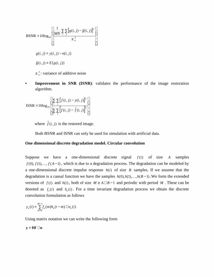
Some characteristic metrics for degradation models
Blurred Signal-to-Noise Ratio (BSNR): a metric that describes the degradation model.
2
2
10
),(),(1
10logBSNRn
i jjigjig
MN
),(),(),( jinjiyjig
)},({),( jigEjig
2n : variance of additive noise
Improvement in SNR (ISNR): validates the performance of the image restorationalgorithm.
i j
i j
jifjif
jiyjif
2
2
10
),(ˆ),(
),(),(
10logISNR
where ),(ˆ jif is the restored image.
Both BSNR and ISNR can only be used for simulation with artificial data.
One dimensional discrete degradation model. Circular convolution
Suppose we have a one-dimensional discrete signal )(if of size A samples
)1(,),1(),0( Afff , which is due to a degradation process. The degradation can be modeled by
a one-dimensional discrete impulse response )(ih of size B samples. If we assume that the
degradation is a causal function we have the samples )1(,),1(),0( Bhhh .We form the extended
versions of )(if and )(ih , both of size 1 BAM and periodic with period M . These can be
denoted as )(ife and )(ihe . For a time invariant degradation process we obtain the discrete
convolution formulation as follows
1
0)()()()(
M
meeee inmihmfiy
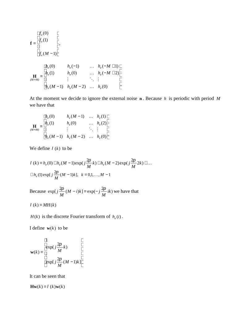
Using matrix notation we can write the following form
nHfy
)1(
)1(
)0(
Mf
f
f
e
e
e
f ,
)0()2()1(
)2()0()1(
)1()1()0(
eee
eee
eee
M)(M
hMhMh
Mhhh
Mhhh
H
At the moment we decide to ignore the external noise n . Because h is periodic with period M
we have that
)0()2()1(
)2()0()1(
)1()1()0(
eee
eee
eee
M)(M
hMhMh
hhh
hMhh
H
We define )(k to be
)22
exp()2()2
exp()1()0()( kM
jMhkM
jMhhk eee
1,,1,0],)1(2
exp[)1( MkkMM
jhe
Because )2
exp(])(2
exp[ ikM
jkiMM
j
we have that
)()( kMHk
)(kH is the discrete Fourier transform of )(ihe .
I define )(kw to be
])1(2
exp[
)2
exp(
1
)(
kMM
j
kM
jk
w
It can be seen that
)()()( kkk wHw
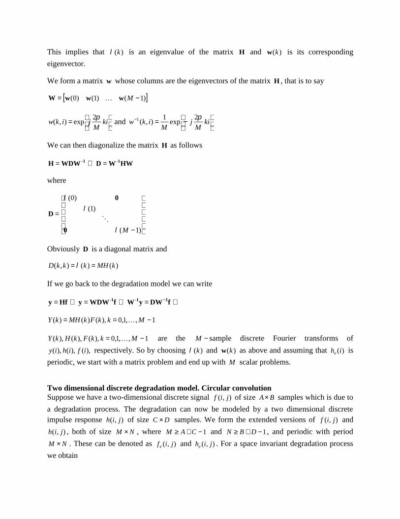
This implies that )(k is an eigenvalue of the matrix H and )(kw is its corresponding
eigenvector.
We form a matrix w whose columns are the eigenvectors of the matrix H , that is to say
)1()1()0( MwwwW
ki
Mjikw
2exp),( and
ki
Mj
Mikw
2exp
1),(1
We can then diagonalize the matrix H as follows
HWWDWDWH -1-1
where
)1(
)1(
)0(
M
0
0
D
Obviously D is a diagonal matrix and
)()(),( kMHkkkD
If we go back to the degradation model we can write
fDWyWfWDWyHfy 1-1-1
1,,1,0),()()( MkkFkMHkY
1,,1,0),(),(),( MkkFkHkY are the M sample discrete Fourier transforms of
),(),(),( ifihiy respectively. So by choosing )(k and )(kw as above and assuming that )(ihe is
periodic, we start with a matrix problem and end up with M scalar problems.
Two dimensional discrete degradation model. Circular convolutionSuppose we have a two-dimensional discrete signal ),( jif of size BA samples which is due to
a degradation process. The degradation can now be modeled by a two dimensional discreteimpulse response ),( jih of size DC samples. We form the extended versions of ),( jif and
),( jih , both of size NM , where 1 CAM and 1 DBN , and periodic with period
NM . These can be denoted as ),( jife and ),( jihe . For a space invariant degradation process
we obtain
1
0
1
0),(),(),(),(
M
mee
N
nee jinnjmihnmfjiy
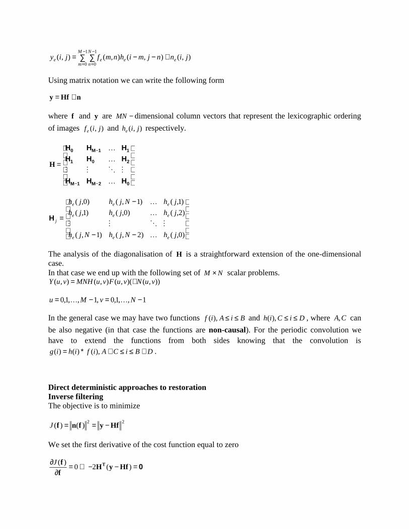
Using matrix notation we can write the following form
nHfy
where f and y are MN dimensional column vectors that represent the lexicographic ordering
of images ),( jife and ),( jihe respectively.
02M1M
201
11M0
HHH
HHHHHH
H
)0,()2,()1,(
)2,()0,()1,(
)1,()1,()0,(
jhNjhNjh
jhjhjh
jhNjhjh
eee
eee
eee
j
H
The analysis of the diagonalisation of H is a straightforward extension of the one-dimensionalcase.In that case we end up with the following set of NM scalar problems.
)),()(,(),(),( vuNvuFvuMNHvuY
1,,1,0,1,,1,0 NvMu
In the general case we may have two functions BiAif ),( and DiCih ),( , where CA, can
be also negative (in that case the functions are non-causal). For the periodic convolution wehave to extend the functions from both sides knowing that the convolution is
DBiCAifihig ),()()( .
Direct deterministic approaches to restorationInverse filteringThe objective is to minimize
22)()( Hfyfnf J
We set the first derivative of the cost function equal to zero
0
)(20
)(HfyH
ff TJ
yHHHf T-1T )(
If NM and 1H exists then
yHf -1
According to the previous analysis if H (and therefore -1H ) is block circulant the above problemcan be solved as a set of NM scalar problems as follows
21
2),(
),(),(),(
),(
),(),(),(
vuH
vuYvuHjif
vuH
vuYvuHvuF
Computational issues concerning inverse filtering
(I) Suppose first that the additive noise ),( jin is negligible. A problem arises if ),( vuH
becomes very small or zero for some point ),( vu or for a whole region in the ),( vu plane.
In that region inverse filtering cannot be applied. Note that in most real applications),( vuH drops off rapidly as a function of distance from the origin. The solution is that if
these points are known they can be neglected in the computation of ),( vuF .
(II) In the presence of external noise we have that
2),(
),(),(),(),(ˆ
vuH
vuNvuYvuHvuF
22),(
),(),(
),(
),(),(
vuH
vuNvuH
vuH
vuYvuH
),(
),(),(),(ˆ
vuH
vuNvuFvuF
If ),( vuH becomes very small, the term ),( vuN dominates the result. The solution is
again to carry out the restoration process in a limited neighborhood about the originwhere ),( vuH is not very small. This procedure is called pseudoinverse filtering. In that
case we set
TvuH
TvuHvuH
vuYvuH
vuF
),(0
),(),(
),(),(
),(ˆ2
The threshold T is defined by the user. In general, the noise may very well possess largecomponents at high frequencies ),( vu , while ),( vuH and ),( vuY normally will be
dominated by low frequency components.
Constrained least squares (CLS) restorationIt refers to a very large number of restoration algorithms.
The problem can be formulated as follows.
minimize
22)()( Hfyfnf J
subject to
2Cf
where Cf is a high pass filtered version of the image. The idea behind the above constraint isthat the highpass version of the image contains a considerably large amount of noise!Algorithms of the above type can be handled using optimization techniques. Constrained leastsquares (CLS) restoration can be formulated by choosing an f to minimize the Lagrangian
22min CfHfy
Typical choice for C is the 2-D Laplacian operator given by
00.025.000.0
25.000.125.0
00.025.000.0
C
represents either a Lagrange multiplier or a fixed parameter known as regularisation
parameter and it controls the relative contribution between the term2
Hfy and the term2
Cf . The minimization of the above leads to the following estimate for the original image
yHCCHHf TTT 1
Computational issues concerning the CLS method
(I) Choice of
The problem of the choice of has been attempted in a large number of studies anddifferent techniques have been proposed. One possible choice is based on a set theoretic
approach: a restored image is approximated by an image which lies in the intersection ofthe two ellipsoids defined by
}|{ 22EQ Hfyfy|f and
}|{ 22 CfffQ
The center of one of the ellipsoids which bounds the intersection of y|fQ and fQ , is given
by the equation
yHCCHHf TTT 1
with 2)/( E . Another problem is then the choice of 2E and 2 . One choice could be
BSNR
1
Comments
With larger values of , and thus more regularisation, the restored image tends to havemore ringing. With smaller values of , the restored image tends to have more amplifiednoise effects. The variance and bias of the error image in frequency domain are
M
u
N
vn
vuCvuH
vuHVar
0 0222
22
),(),(
),()(
1
0
1
0222
4222
),(),(
),(),()(
M
u
N
vn
vuCvuH
vuCvuFBias
The minimum MSE is encountered close to the intersection of the above functions.
A good choice of is one that gives the best compromise between the variance and biasof the error image.
Iterative deterministic approaches to restorationThey refer to a large class of methods that have been investigated extensively over the lastdecades. They possess the following advantages.
There is no need to explicitly implement the inverse of an operator. The restoration processis monitored as it progresses. Termination of the algorithm may take place beforeconvergence.
The effects of noise can be controlled in each iteration.
The algorithms used can be spatially adaptive.
The problem specifications are very flexible with respect to the type of degradation.Iterative techniques can be applied in cases of spatially varying or nonlinear degradationsor in cases where the type of degradation is completely unknown (blind restoration).
In general, iterative restoration refers to any technique that attempts to minimize a function of theform
)(fM
using an updating rule for the partially restored image.
Least squares iteration
In that case we seek for a solution that minimizes the function
2Hfyf )(M
A necessary condition for )(fM to have a minimum is that its gradient with respect to f is equal
to zero. This gradient is given below
Hf)HyHfff TT
f
(2)(
)(M
M
and by using the steepest descent type of optimization we can formulate an iterative rule asfollows:
yHf T0
kTT
kT
kk
kk fHHIyHHfyHf
f
fff )()(
)(
M
1k
Constrained least squares iteration
In this method we attempt to solve the problem of constrained restoration iteratively. As alreadymentioned the following functional is minimized
22),( CfHfyf M
The necessary condition for a minimum is that the gradient of ),( fM is equal to zero. That
gradient is
])[(2),()( yHfCCHHff TTTf M
The initial estimate and the updating rule for obtaining the restored image are now given by
yHf T0
])([ kTTT
k fCCHHyHff 1k
It can be proved that the above iteration (known as Iterative CLS or Tikhonov-Miller Method)converges if
max
20
where max is the maximum eigenvalue of the matrix
)( CCHH TT
If the matrices H and C are block-circulant the iteration can be implemented in the frequencydomain.
Projection onto convex sets (POCS)
The set-based approach described previously can be generalized so that any number of priorconstraints can be imposed as long as the constraint sets are closed convex.
If the constraint sets have a non-empty intersection, then a solution that belongs to theintersection set can be found by the method of POCS. Any solution in the intersection set isconsistent with the a priori constraints and therefore it is a feasible solution. Let mQQQ ,,, 21 be
closed convex sets in a finite dimensional vector space, with mPPP ,,, 21 their respective
projectors. The iterative procedure
k1k ff mPPP ,21
converges to a vector that belongs to the intersection of the sets miQi ,,2,1, , for any starting
vector 0f . An iteration of the form k1k ff 21PP can be applied in the problem described
previously, where we seek for an image which lies in the intersection of the two ellipsoidsdefined by
}|{ 22EQ Hfyfy|f and }|{ 22 CfffQ
The respective projections f1P and f2P are defined by
)(1
111 HfyHHHIff TT
λλP

fCCCCIIf TT ][1
222
λλP
Spatially adaptive iteration
The functional to be minimized takes the form
2W1W CfHfyf22
),( M
where
Hf)yWHf)yHfy 1T
1W ((2
Cf)WCf)Cf 2T
2W ((2
21 WW , are diagonal matrices, the choice of which can be justified in various ways. The entries in
both matrices are non-negative values and less than or equal to unity. In that case
yWHfCWCHWHff 1T
2T
1T
f )(),()( M
A more specific case is
WCfHfyf22
),( M
where the weighting matrix is incorporated only in the regularization term. This method isknown as weighted regularised image restoration. The entries in matrix W will be chosen sothat the high-pass filter is only effective in the areas of low activity and a very little smoothingtakes place in the edge areas.
Robust functionals
Robust functionals allow for the efficient supression of a wide variety of noise processes andpermit the reconstruction of sharper edges than their quadratic counterparts. We are seeking tominimize
CfHfyf xn RRM )(),(
()(), xn RR are referred to as residual and stabilizing functionals respectively.
Computational issues concerning iterative techniques
(I) Convergence
The contraction mapping theorem usually serves as a basis for establishingconvergence of iterative algorithms. According to it iteration
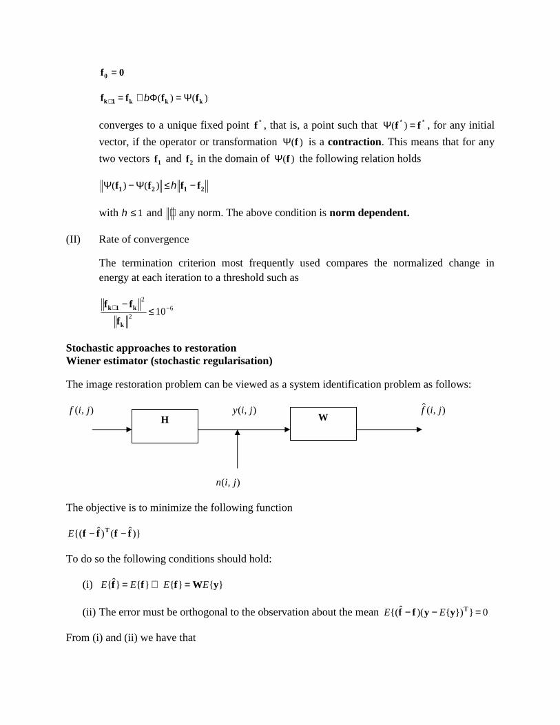
0f0
)()( kkk ffff 1k
converges to a unique fixed point f , that is, a point such that ff )( , for any initial
vector, if the operator or transformation )(f is a contraction. This means that for any
two vectors 1f and 2f in the domain of )(f the following relation holds
2121 ffff )()(
with 1 and any norm. The above condition is norm dependent.
(II) Rate of convergence
The termination criterion most frequently used compares the normalized change inenergy at each iteration to a threshold such as
62
2
10
k
k1k
f
ff
Stochastic approaches to restorationWiener estimator (stochastic regularisation)
The image restoration problem can be viewed as a system identification problem as follows:
),( jif ),( jiy ),(ˆ jif
),( jin
The objective is to minimize the following function
)}ˆ()ˆ{( ffff T E
To do so the following conditions should hold:
(i) }{}{}{}ˆ{ yWfff EEEE
(ii) The error must be orthogonal to the observation about the mean 0}}){)(ˆ{( Tyyff EE
From (i) and (ii) we have that
H W
0}}){)({( TyyfWy EE 0}}){)(}{}{{( TyyfyWfWy EEEE
0}}){})]({(}){({[ TyyffyyW EEEE
If }{~ yyy E and }{~
fff E then
0}~)~~{( TyfyWE yfyy
TTTT RWRyfyyWyfyyW ~~~~}~~{}~~{}~~
{}~~{ EEEE
If the original and the degraded image are both zero mean then yyyy RR ~~ and fyyf RR ~~ . In that
case we have that fyyy RWR . If we go back to the degradation model and find the
autocorrelation matrix of the degraded image then we get that
TTTT nHfynHfy
yynnT
ffT RRHHRyy }{E
fyT
ffT RHRfy }{E
From the above we get the following results
11 )( nnT
ffT
ffyyfy RHHRHRRRW
yRHHRHRf nnT
ffT
ff1 )(ˆ
Note that knowledge of ffR and nnR is assumed. In frequency domain
),(),(),(
),(),(),(
2vuSvuHvuS
vuHvuSvuW
nnff
ff
),(),(),(),(
),(),(),(ˆ
2vuY
vuSvuHvuS
vuHvuSvuF
nnff
ff
Computational issues
The noise variance has to be known, otherwise it is estimated from a flat region of the observedimage. In practical cases where a single copy of the degraded image is available, it is quitecommon to use ),( vuS yy as an estimate of ),( vuS ff . This is very often a poor estimate.
Wiener smoothing filter
In the absence of any blur, 1),( vuH and
1)(
)(
),(),(
),(),(
SNR
SNR
vuSvuS
vuSvuW
nnff
ff
(i) 1),(1)( vuWSNR
(ii) )(),(1)( SNRvuWSNR
)(SNR is high in low spatial frequencies and low in high spatial frequencies so ),( vuW can be
implemented with a lowpass (smoothing) filter.
Relation with inverse filtering
If),(
1),(0),(
vuHvuWvuSnn which is the inverse filter
If 0),( vuS nn
0),(0
0),(),(
1
),(lim0
vuH
vuHvuH
vuWnnS
which is the pseudoinverse filter.
Iterative Wiener filters
They refer to a class of iterative procedures that successively use the Wiener filtered signal as animproved prototype to update the covariance estimates of the original image as follows.
Step 0: Initial estimate of ffR
}{)0( Tyyff yyRR E
Step 1: Construct the thi restoration filter
1 ))(()()1( nnT
ffT
ff RHHRHRW iii
Step 2: Obtain the th)1( i estimate of the restored image
yWf )1()1(ˆ ii
Step 3: Use )1(ˆ if to compute an improved estimate of ffR given by
)}1(ˆ)1(ˆ{)1( iiEi Tff ffR
Step 4: Increase i and repeat steps 1,2,3,4.
UNIT IV
IMAGE SEGEMENTATION
Segmentation was used to identify the object of image that we are interested.
We have three approaches to do it. The first is Edge detection. The second is to use threshold. The third isthe region-based segmentation. It does not mean that these three of that method can solve all of theproblems that we met, but these approaches are the basic methods in segmentation.
Introduction:
We first discuss from the case of the monochrome and static images. The fundamental problem insegmentation is to partition an image into regions. Segmentation algorithms for monochrome images aregenerally based on one of the following two basic categories. The first one is Edge-based segmentation.The second one is Region-based segmentation. Another method is to use the threshold. It belongs toEdge-based segmentation.There are three goals that we want to achieve:
1. The first one is speed. Because we need to save the time from segmentation and givecomplicate compression more time to process.
2. The second, one is to have a good shape matching even under less computation time.3. The third, one is that the result of segmenting shape will be intact but not fragmentary
which means that we want to have good connectivity.
Edge-Based Segmentation
The focus of this section is on the segmentation methods based on detection in sharp, localchanges in intensity. The three types of image feature in which we are interested are isolatedpoints, lines , and edges. Edge pixels are pixels at which the intensity of an image functionchanges abruptly.
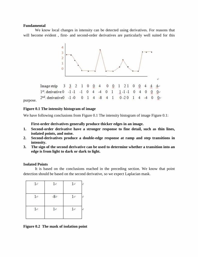
FundamentalWe know local changes in intensity can be detected using derivatives. For reasons that
will become evident , first- and second-order derivatives are particularly well suited for this
purpose.
Figure 0.1 The intensity histogram of image
We have following conclusions from Figure 0.1 The intensity histogram of image Figure 0.1:
First-order derivatives generally produce thicker edges in an image.1. Second-order derivative have a stronger response to fine detail, such as thin lines,
isolated points, and noise.2. Second-derivatives produce a double-edge response at ramp and step transitions in
intensity.3. The sign of the second derivative can be used to determine whether a transition into an
edge is from light to dark or dark to light.
Isolated PointsIt is based on the conclusions reached in the preceding section. We know that point
detection should be based on the second derivative, so we expect Laplacian mask.
Figure 0.2 The mask of isolation point

We can use the mask to scan the all point of image , and count the response of every point, if theresponse of point is greater than T(the threshold we set), we can define the point to 1(light), ifnot, set to 0(dark).
1 if ( , )0 otherwise( , ) R x y TG x y (2.1)
Line DetectionAs discussion in section2.1,we know the second order derivative have stronger response and
to produce thinner lines than 1st derivative. We can get four different direction of mask.
Figure 0.3 Line detection masks.
Let talk about how to use the four masks to decide which direction of mask is better than others.
Let 1R , 2R , 3R and 4R denote the response of the masks in Figure 0.3. If at a point in the image ,
kR > jR ,for all j k. 1R > jR for j=2,3,4,that point is said to be more likely associated with a
line in the direction of mask k.
Edge detection
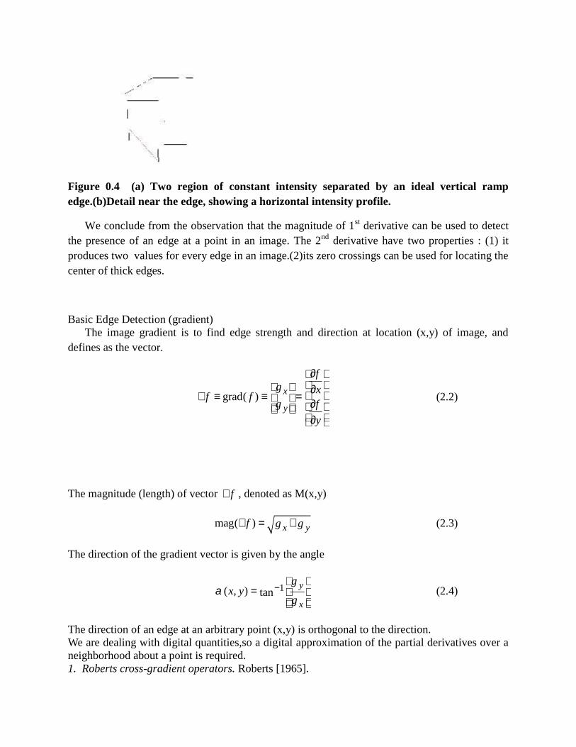
Figure 0.4 (a) Two region of constant intensity separated by an ideal vertical rampedge.(b)Detail near the edge, showing a horizontal intensity profile.
We conclude from the observation that the magnitude of 1st derivative can be used to detectthe presence of an edge at a point in an image. The 2nd derivative have two properties : (1) itproduces two values for every edge in an image.(2)its zero crossings can be used for locating thecenter of thick edges.
Basic Edge Detection (gradient)The image gradient is to find edge strength and direction at location (x,y) of image, and
defines as the vector.
grad( ) x
y
fg x
f fg f
y
(2.2)
The magnitude (length) of vector f , denoted as M(x,y)
mag( ) x yf g g (2.3)
The direction of the gradient vector is given by the angle
1( , ) tany
x
gx y
g
(2.4)
The direction of an edge at an arbitrary point (x,y) is orthogonal to the direction.We are dealing with digital quantities,so a digital approximation of the partial derivatives over aneighborhood about a point is required.1. Roberts cross-gradient operators. Roberts [1965].
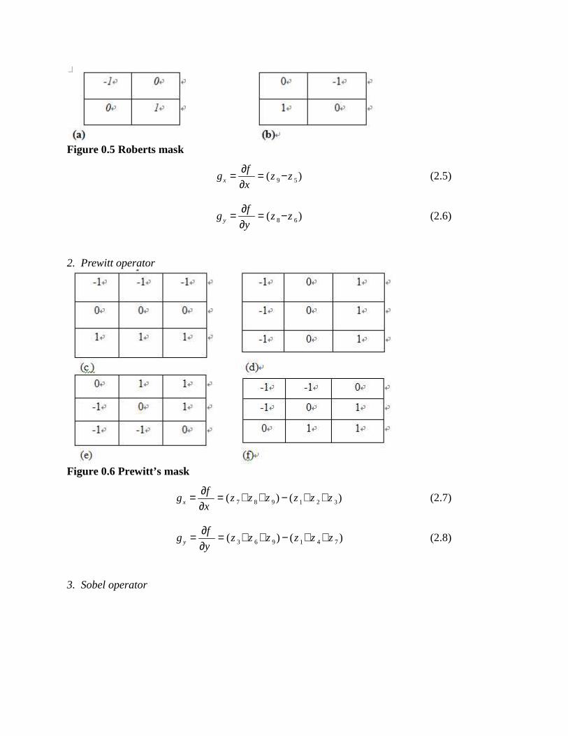
Figure 0.5 Roberts mask
9 5( )x
fg z z
x
(2.5)
8 6( )y
fg z z
y
(2.6)
2. Prewitt operator
Figure 0.6 Prewitt’s mask
7 8 9 1 2 3( ) ( )x
fg z z z z z z
x
(2.7)
3 6 9 1 4 7( ) ( )y
fg z z z z z z
y
(2.8)
3. Sobel operator
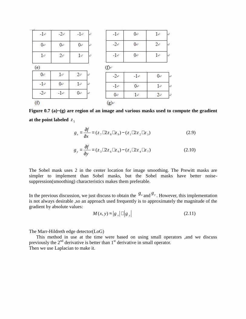
Figure 0.7 (a)~(g) are region of an image and various masks used to compute the gradient
at the point labeled 5z
7 8 9 1 2 3( 2 ) ( 2 )x
fg z z z z z z
x
(2.9)
3 6 9 1 4 7( 2 ) ( 2 )y
fg z z z z z z
y
(2.10)
The Sobel mask uses 2 in the center location for image smoothing. The Prewitt masks aresimpler to implement than Sobel masks, but the Sobel masks have better noise-suppression(smoothing) characteristics makes them preferable.
In the previous discussion, we just discuss to obtain the xg and yg. However, this implementation
is not always desirable ,so an approach used frequently is to approximately the magnitude of thegradient by absolute values:
( , ) x yM x y g g (2.11)
The Marr-Hildreth edge detector(LoG)This method in use at the time were based on using small operators ,and we discuss
previously the 2nd derivative is better than 1st derivative in small operator.Then we use Laplacian to make it.
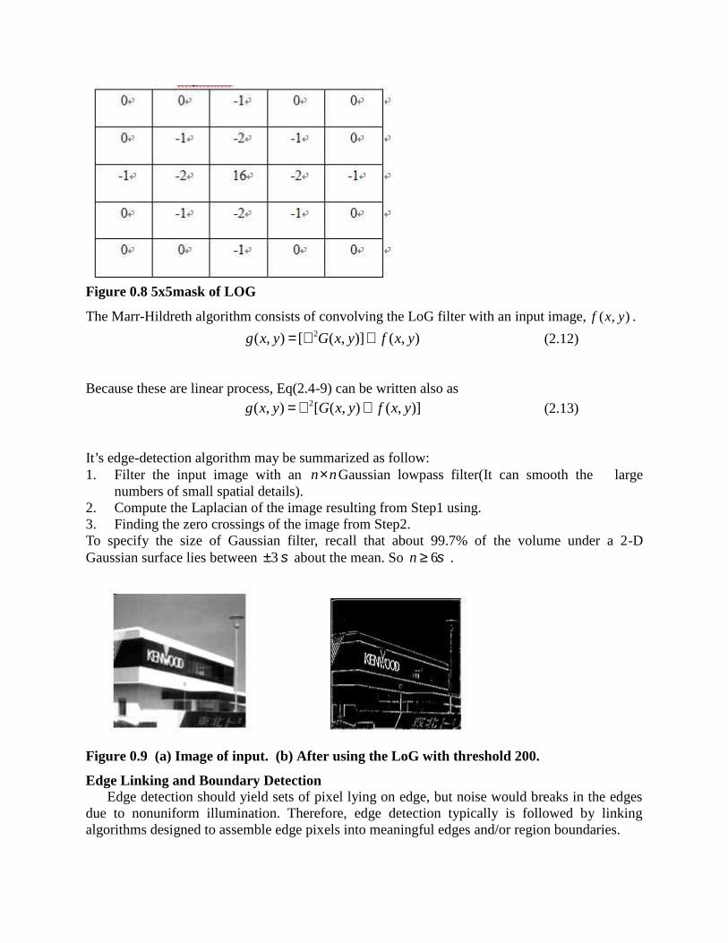
Figure 0.8 5x5mask of LOG
The Marr-Hildreth algorithm consists of convolving the LoG filter with an input image, ( , )f x y .2( , ) [ ( , )] ( , )g x y G x y f x y (2.12)
Because these are linear process, Eq(2.4-9) can be written also as2( , ) [ ( , ) ( , )]g x y G x y f x y (2.13)
It’s edge-detection algorithm may be summarized as follow:1. Filter the input image with an n n Gaussian lowpass filter(It can smooth the large
numbers of small spatial details).2. Compute the Laplacian of the image resulting from Step1 using.3. Finding the zero crossings of the image from Step2.To specify the size of Gaussian filter, recall that about 99.7% of the volume under a 2-DGaussian surface lies between 3 about the mean. So 6n .
Figure 0.9 (a) Image of input. (b) After using the LoG with threshold 200.
Edge Linking and Boundary DetectionEdge detection should yield sets of pixel lying on edge, but noise would breaks in the edges
due to nonuniform illumination. Therefore, edge detection typically is followed by linkingalgorithms designed to assemble edge pixels into meaningful edges and/or region boundaries.
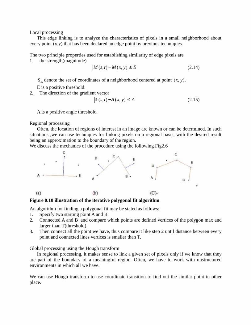
Local processingThis edge linking is to analyze the characteristics of pixels in a small neighborhood about
every point (x,y) that has been declared an edge point by previous techniques.
The two principle properties used for establishing similarity of edge pixels are1. the strength(magnitude)
( , ) ( , )M s t M x y E (2.14)
xyS denote the set of coordinates of a neighborhood centered at point ( , )x y .
E is a positive threshold.2. The direction of the gradient vector
( , ) ( , )s t x y A (2.15)
A is a positive angle threshold.
Regional processingOften, the location of regions of interest in an image are known or can be determined. In such
situations ,we can use techniques for linking pixels on a regional basis, with the desired resultbeing an approximation to the boundary of the region.We discuss the mechanics of the procedure using the following Fig2.6
Figure 0.10 illustration of the iterative polygonal fit algorithm
An algorithm for finding a polygonal fit may be stated as follows:1. Specify two starting point A and B.2. Connected A and B ,and compare which points are defined vertices of the polygon max and
larger than T(threshold).3. Then connect all the point we have, thus compare it like step 2 until distance between every
point and connected lines vertices is smaller than T.
Global processing using the Hough transformIn regional processing, it makes sense to link a given set of pixels only if we know that they
are part of the boundary of a meaningful region. Often, we have to work with unstructuredenvironments in which all we have.
We can use Hough transform to use coordinate transition to find out the similar point in otherplace.
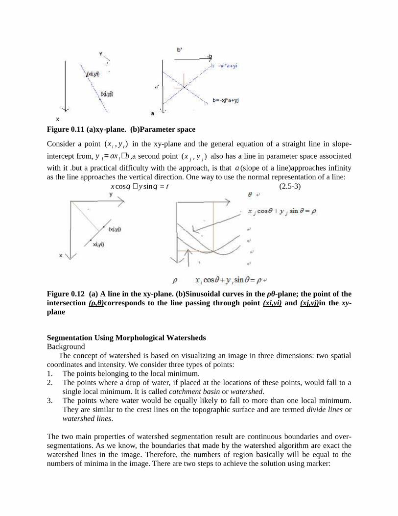
Figure 0.11 (a)xy-plane. (b)Parameter space
Consider a point ( , )i ix y in the xy-plane and the general equation of a straight line in slope-
intercept from, i iy ax b ,a second point ( , )j jx y also has a line in parameter space associated
with it .but a practical difficulty with the approach, is that a (slope of a line)approaches infinityas the line approaches the vertical direction. One way to use the normal representation of a line:
cos sinx y (2.5-3)
Figure 0.12 (a) A line in the xy-plane. (b)Sinusoidal curves in the ρθ-plane; the point of theintersection (ρ,θ)corresponds to the line passing through point (xi,yi) and (xj,yj)in the xy-plane
Segmentation Using Morphological WatershedsBackground
The concept of watershed is based on visualizing an image in three dimensions: two spatialcoordinates and intensity. We consider three types of points:1. The points belonging to the local minimum.2. The points where a drop of water, if placed at the locations of these points, would fall to a
single local minimum. It is called catchment basin or watershed.3. The points where water would be equally likely to fall to more than one local minimum.
They are similar to the crest lines on the topographic surface and are termed divide lines orwatershed lines.
The two main properties of watershed segmentation result are continuous boundaries and over-segmentations. As we know, the boundaries that made by the watershed algorithm are exact thewatershed lines in the image. Therefore, the numbers of region basically will be equal to thenumbers of minima in the image. There are two steps to achieve the solution using marker:
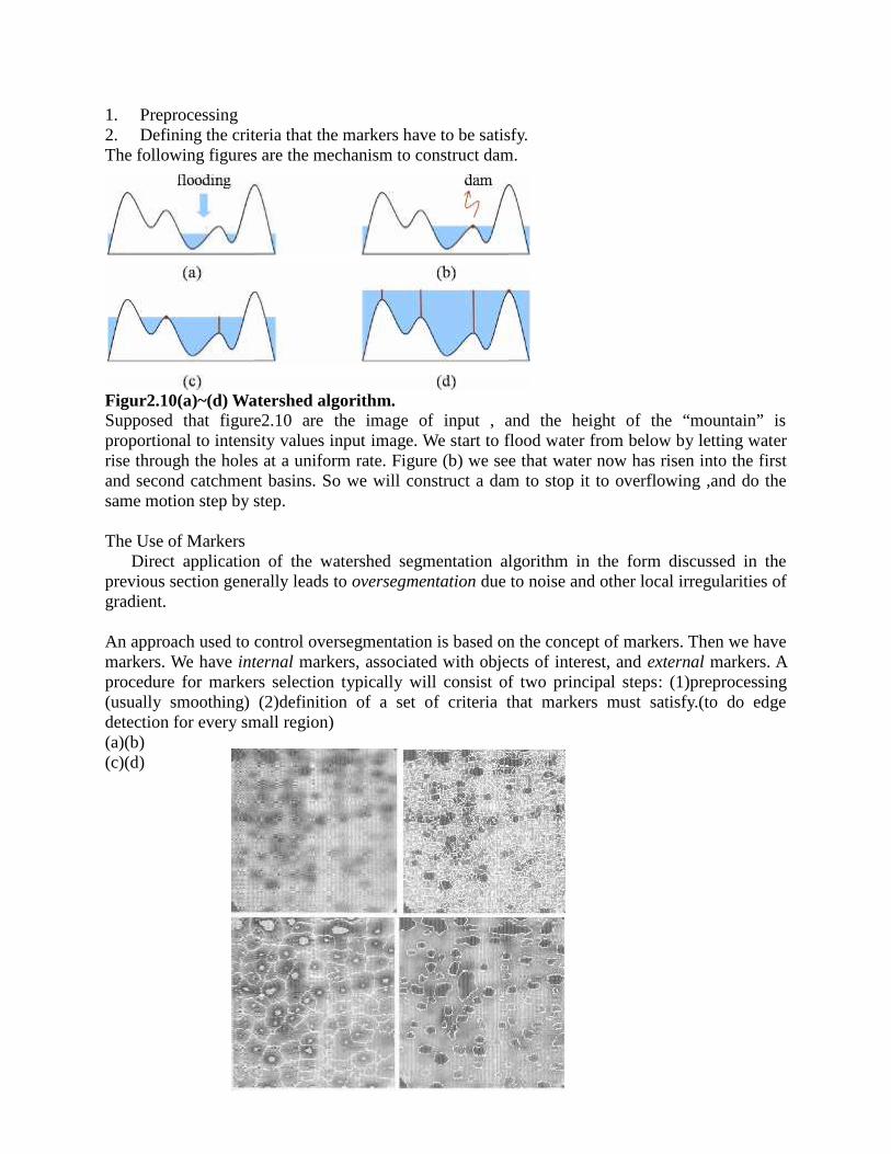
1. Preprocessing2. Defining the criteria that the markers have to be satisfy.The following figures are the mechanism to construct dam.
Figur2.10(a)~(d) Watershed algorithm.Supposed that figure2.10 are the image of input , and the height of the “mountain” isproportional to intensity values input image. We start to flood water from below by letting waterrise through the holes at a uniform rate. Figure (b) we see that water now has risen into the firstand second catchment basins. So we will construct a dam to stop it to overflowing ,and do thesame motion step by step.
The Use of MarkersDirect application of the watershed segmentation algorithm in the form discussed in the
previous section generally leads to oversegmentation due to noise and other local irregularities ofgradient.
An approach used to control oversegmentation is based on the concept of markers. Then we havemarkers. We have internal markers, associated with objects of interest, and external markers. Aprocedure for markers selection typically will consist of two principal steps: (1)preprocessing(usually smoothing) (2)definition of a set of criteria that markers must satisfy.(to do edgedetection for every small region)(a)(b)(c)(d)
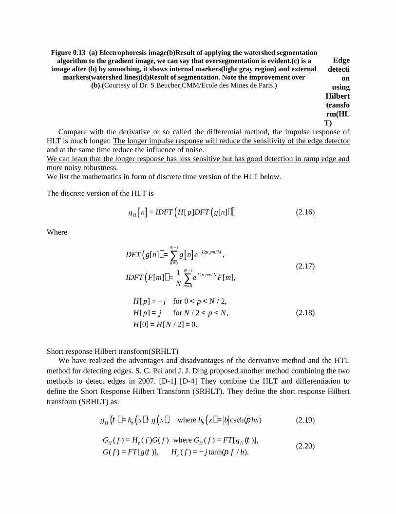
Edgedetecti
onusing
Hilberttransform(HL
T)Compare with the derivative or so called the differential method, the impulse response of
HLT is much longer. The longer impulse response will reduce the sensitivity of the edge detectorand at the same time reduce the influence of noise.We can learn that the longer response has less sensitive but has good detection in ramp edge andmore noisy robustness.We list the mathematics in form of discrete time version of the HLT below.
The discrete version of the HLT is
[ ] [ ]Hg n IDFT H p DFT g n (2.16)
Where
12 /
0
12 /
0
[ ] ,
1[ ] [ ],
Nj pm M
n
Nj pm N
m
DFT g n g n e
IDFT F m e F mN
(2.17)
[ ] for 0 / 2,
[ ] for / 2 ,
[0] [ / 2] 0.
H p j p N
H p j N p N
H H N
(2.18)
Short response Hilbert transform(SRHLT)We have realized the advantages and disadvantages of the derivative method and the HTL
method for detecting edges. S. C. Pei and J. J. Ding proposed another method combining the twomethods to detect edges in 2007. [D-1] [D-4] They combine the HLT and differentiation todefine the Short Response Hilbert Transform (SRHLT). They define the short response Hilberttransform (SRHLT) as:
, where csch( )H b bg h x g x h x b bx (2.19)
( ) ( ) ( ) where ( ) [ ( )],
( ) [ ( )], ( ) tanh( / ).H b H H
b
G f H f G f G f FT g
G f FT g H f j f b
(2.20)
Figure 0.13 (a) Electrophoresis image(b)Result of applying the watershed segmentationalgorithm to the gradient image, we can say that oversegmentation is evident.(c) is a
image after (b) by smoothing, it shows internal markers(light gray region) and externalmarkers(watershed lines)(d)Result of segmentation. Note the improvement over
(b).(Courtesy of Dr. S.Beucher,CMM/Ecole des Mines de Paris.)
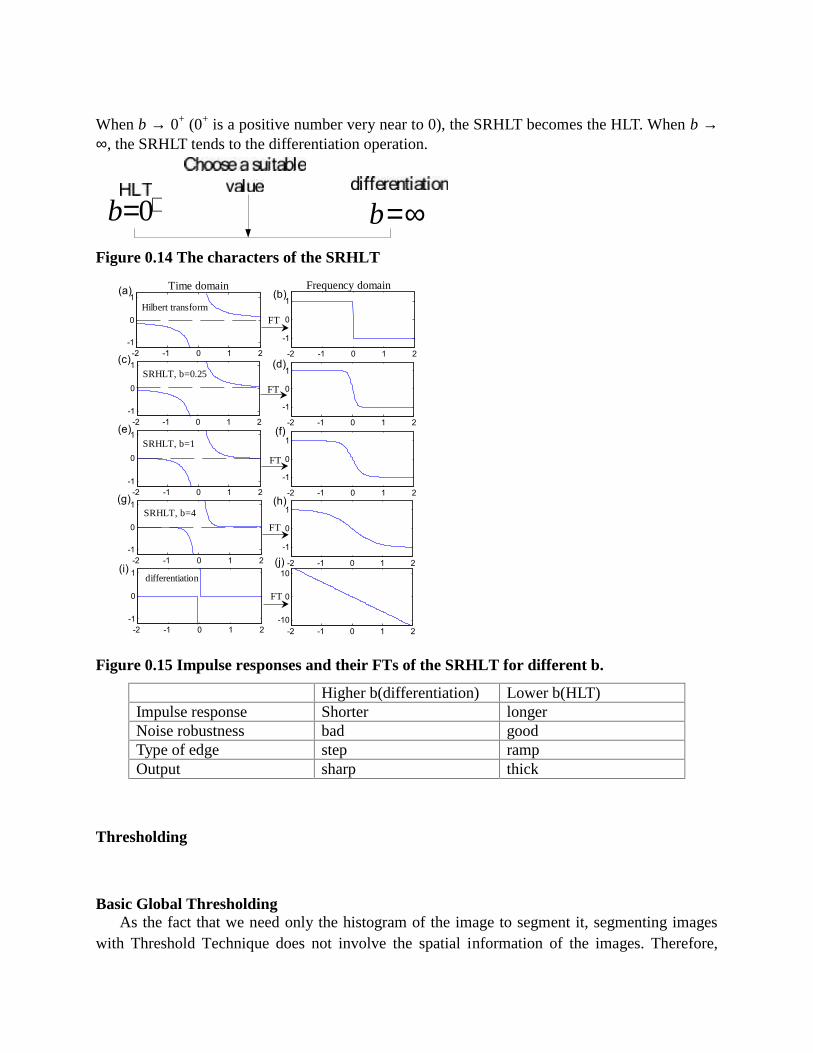
When b 0+ (0+ is a positive number very near to 0), the SRHLT becomes the HLT. When b , the SRHLT tends to the differentiation operation.
b0b Figure 0.14 The characters of the SRHLT
Figure 0.15 Impulse responses and their FTs of the SRHLT for different b.
Higher b(differentiation) Lower b(HLT)Impulse response Shorter longerNoise robustness bad goodType of edge step rampOutput sharp thick
Thresholding
Basic Global ThresholdingAs the fact that we need only the histogram of the image to segment it, segmenting images
with Threshold Technique does not involve the spatial information of the images. Therefore,
-2 -1 0 1 2-1
0
1
-2 -1 0 1 2
-1
0
1
-2 -1 0 1 2-1
0
1
-2 -1 0 1 2-10
0
10
-2 -1 0 1 2-1
0
1
-2 -1 0 1 2
-1
0
1
-2 -1 0 1 2-1
0
1
-2 -1 0 1 2
-1
0
1
-2 -1 0 1 2-1
0
1
-2 -1 0 1 2
-1
0
1
(a) (b)
(c) (d)
(e) (f)
(g) (h)
(i) (j)
Time domain Frequency domain
Hilbert transform
differentiation
SRHLT, b=0.25
SRHLT, b=1
SRHLT, b=4
FT
FT
FT
FT
FT
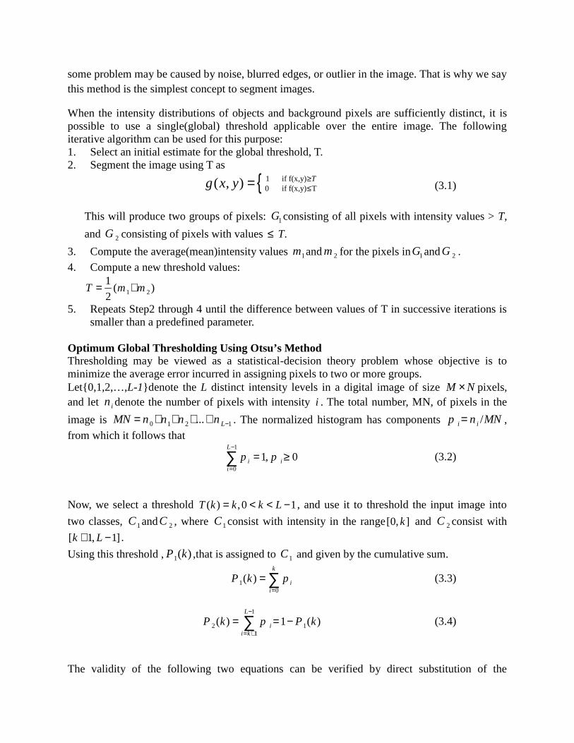
some problem may be caused by noise, blurred edges, or outlier in the image. That is why we saythis method is the simplest concept to segment images.
When the intensity distributions of objects and background pixels are sufficiently distinct, it ispossible to use a single(global) threshold applicable over the entire image. The followingiterative algorithm can be used for this purpose:1. Select an initial estimate for the global threshold, T.2. Segment the image using T as
1 if f(x,y)0 if f(x,y) T( , ) Tg x y
(3.1)
This will produce two groups of pixels: 1G consisting of all pixels with intensity values > T,
and 2G consisting of pixels with values T.
3. Compute the average(mean)intensity values 1m and 2m for the pixels in 1G and 2G .
4. Compute a new threshold values:
1 2
1( )
2T m m
5. Repeats Step2 through 4 until the difference between values of T in successive iterations issmaller than a predefined parameter.
Optimum Global Thresholding Using Otsu’s MethodThresholding may be viewed as a statistical-decision theory problem whose objective is tominimize the average error incurred in assigning pixels to two or more groups.Let{0,1,2,…,L-1}denote the L distinct intensity levels in a digital image of size M N pixels,and let in denote the number of pixels with intensity i . The total number, MN, of pixels in the
image is 0 1 2 1... LMN n n n n . The normalized histogram has components /i ip n MN ,
from which it follows that1
0
1, 0L
i ii
p p
(3.2)
Now, we select a threshold ( ) ,0 1T k k k L , and use it to threshold the input image into
two classes, 1C and 2C , where 1C consist with intensity in the range[0, ]k and 2C consist with
[ 1, 1]k L .
Using this threshold , 1( )P k ,that is assigned to 1C and given by the cumulative sum.
10
( )k
ii
P k p
(3.3)
1
2 11
( ) 1 ( )L
ii k
P k p P k
(3.4)
The validity of the following two equations can be verified by direct substitution of the
preceding result:
1 1 2 2 GP m P m m (3.5)
1 2+ =1P P (3.6)
In order to evaluate the “goodness” of the threshold at level k we use the normalized,dimensionless metric
2B
2G
( )=
k
(3.7)
Where 2G is the global variance
1
22G
0
=L
G ii
i m p
(3.8)
And 2B is the between-class variance, define as :
2 2 2B 1 1 2 2( ) ( )G GP m m P m m (3.9)
2 2B 1 2 1 2( ) ( )k P P m m
21
1 1
( ( ) ( ))
( )(1 ( ))Gm P k m k
P k P k
(3.10)
Indicating that the between-class variance and is a measure of separability between class.
Then, the optimum threshold is the value, k ,that maximizes 2B ( )k
2 2B B
1( ) max ( )
o k Lk k
(3.11)
In other word, to find k we simply evaluate (2.7-11) for all integer values of kOnce k has been obtain, the input image ( , )f x y is segmented as before:
1 if f(x,y) k*0 if f(x,y) k*( , )g x y
(3.12)
For x = 0,1,2,…,M-1 and y = 0,1,2…,N-1. This measure has values in the range0 ( *) 1k (3.13)
Using image Smoothing/Edge to improve Global ThresholdCompare the difference between preprocess of smoothing and Edge detection.
Smoothing Edge detectionWhat situation is moresuitable for the method
Large object we areinterested.
Small object we areinterested
Multiple ThresholdFor three classes consisting of three intensity intervals, the between-class variance is given by:
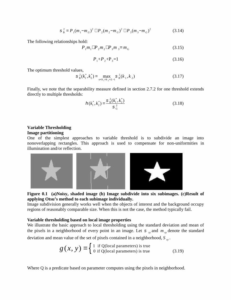
2 2 2 2B 1 1 2 2 3 3( ) ( ) ( )G G GP m m P m m P m m (3.14)
The following relationships hold:
1 1 2 2 3 3 GP m P m P m m (3.15)
1 2 3+ +P =1P P (3.16)
The optimum threshold values,
1 2
2 * * 2B 1 2 B 1 2
1( , ) max ( , )
o k k Lk k k k
(3.17)
Finally, we note that the separability measure defined in section 2.7.2 for one threshold extendsdirectly to multiple thresholds:
2 * ** * B 1 21 2 2
G
( , )( , )
k kk k
(3.18)
Variable ThresholdingImage partitioningOne of the simplest approaches to variable threshold is to subdivide an image intononoverlapping rectangles. This approach is used to compensate for non-uniformities inillumination and/or reflection.
Figure 0.1 (a)Noisy, shaded image (b) Image subdivide into six subimages. (c)Result ofapplying Otsu’s method to each subimage individually.Image subdivision generally works well when the objects of interest and the background occupyregions of reasonably comparable size. When this is not the case, the method typically fail.
Variable thresholding based on local image propertiesWe illustrate the basic approach to local thresholding using the standard deviation and mean ofthe pixels in a neighborhood of every point in an image. Let xy and xym denote the standard
deviation and mean value of the set of pixels contained in a neighborhood, xyS .
1 if Q(local parameters) is true0 if Q(local parameters) is true( , )g x y (3.19)
Where Q is a predicate based on parameter computes using the pixels in neighborhood.
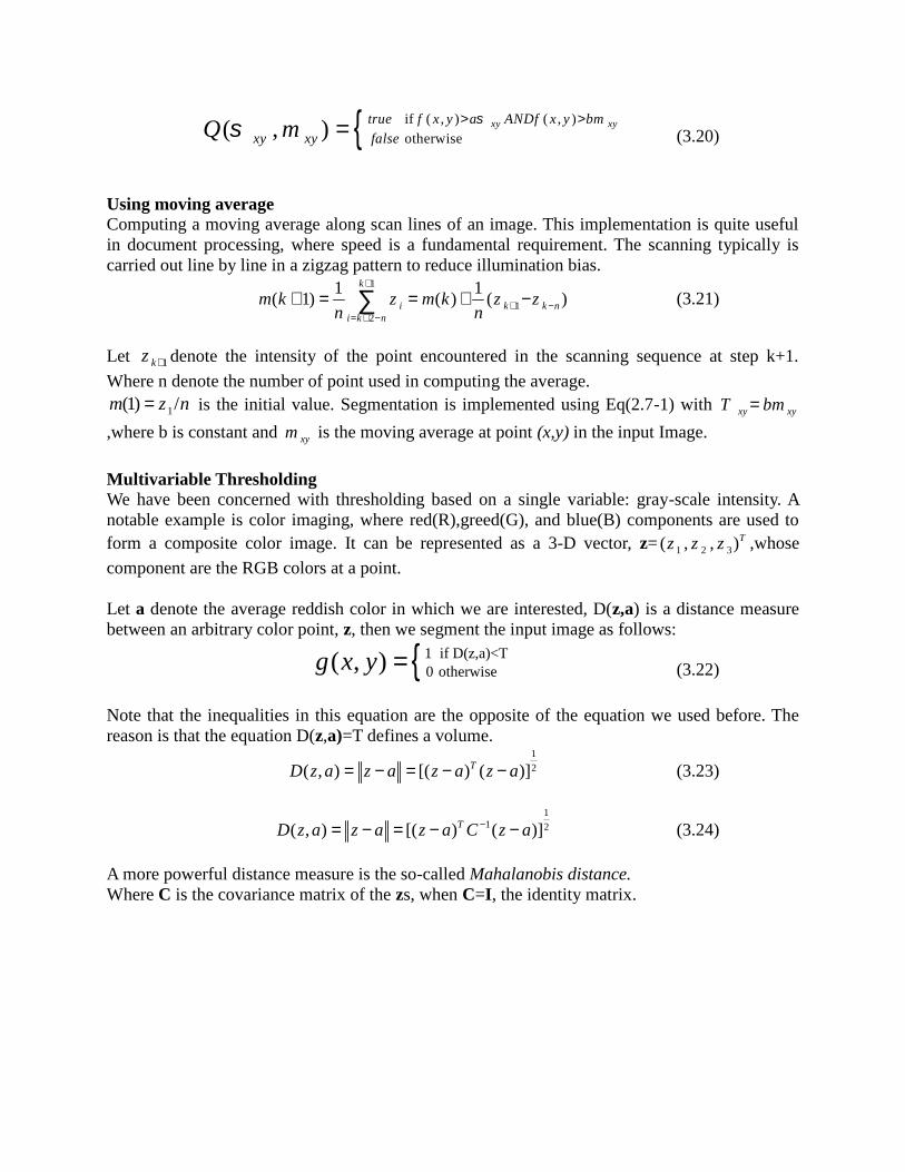
if ( , ) ( , ) otherwise( , ) xy xytrue f x y a ANDf x y bm
xy xy falseQ m (3.20)
Using moving averageComputing a moving average along scan lines of an image. This implementation is quite usefulin document processing, where speed is a fundamental requirement. The scanning typically iscarried out line by line in a zigzag pattern to reduce illumination bias.
1
12
1 1( 1) ( ) ( )
k
i k k ni k n
m k z m k z zn n
(3.21)
Let 1kz denote the intensity of the point encountered in the scanning sequence at step k+1.
Where n denote the number of point used in computing the average.
1(1) /m z n is the initial value. Segmentation is implemented using Eq(2.7-1) with xy xyT bm
,where b is constant and xym is the moving average at point (x,y) in the input Image.
Multivariable ThresholdingWe have been concerned with thresholding based on a single variable: gray-scale intensity. Anotable example is color imaging, where red(R),greed(G), and blue(B) components are used toform a composite color image. It can be represented as a 3-D vector, z= 1 2 3( , , )Tz z z ,whose
component are the RGB colors at a point.
Let a denote the average reddish color in which we are interested, D(z,a) is a distance measurebetween an arbitrary color point, z, then we segment the input image as follows:
1 if D(z,a)<T0 otherwise( , )g x y (3.22)
Note that the inequalities in this equation are the opposite of the equation we used before. Thereason is that the equation D(z,a)=T defines a volume.
1
2( , ) [( ) ( )]TD z a z a z a z a (3.23)
11 2( , ) [( ) ( )]TD z a z a z a C z a (3.24)
A more powerful distance measure is the so-called Mahalanobis distance.Where C is the covariance matrix of the zs, when C=I, the identity matrix.
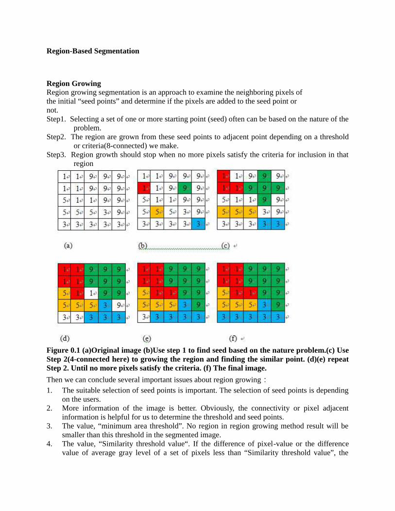
Region-Based Segmentation
Region GrowingRegion growing segmentation is an approach to examine the neighboring pixels ofthe initial “seed points” and determine if the pixels are added to the seed point ornot.Step1. Selecting a set of one or more starting point (seed) often can be based on the nature of the
problem.Step2. The region are grown from these seed points to adjacent point depending on a threshold
or criteria(8-connected) we make.Step3. Region growth should stop when no more pixels satisfy the criteria for inclusion in that
region
Figure 0.1 (a)Original image (b)Use step 1 to find seed based on the nature problem.(c) UseStep 2(4-connected here) to growing the region and finding the similar point. (d)(e) repeatStep 2. Until no more pixels satisfy the criteria. (f) The final image.
Then we can conclude several important issues about region growing:1. The suitable selection of seed points is important. The selection of seed points is depending
on the users.2. More information of the image is better. Obviously, the connectivity or pixel adjacent
information is helpful for us to determine the threshold and seed points.3. The value, “minimum area threshold”. No region in region growing method result will be
smaller than this threshold in the segmented image.4. The value, “Similarity threshold value“. If the difference of pixel-value or the difference
value of average gray level of a set of pixels less than “Similarity threshold value”, the
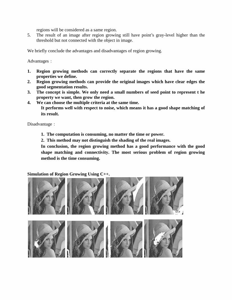
regions will be considered as a same region.5. The result of an image after region growing still have point’s gray-level higher than the
threshold but not connected with the object in image.
We briefly conclude the advantages and disadvantages of region growing.
Advantages:
1. Region growing methods can correctly separate the regions that have the sameproperties we define.
2. Region growing methods can provide the original images which have clear edges thegood segmentation results.
3. The concept is simple. We only need a small numbers of seed point to represent t heproperty we want, then grow the region.
4. We can choose the multiple criteria at the same time.It performs well with respect to noise, which means it has a good shape matching ofits result.
Disadvantage:
1. The computation is consuming, no matter the time or power.2. This method may not distinguish the shading of the real images.In conclusion, the region growing method has a good performance with the goodshape matching and connectivity. The most serious problem of region growingmethod is the time consuming.
Simulation of Region Growing Using C++.
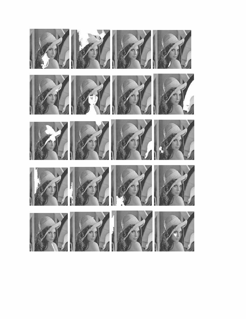

Figure 0.2 Lena image after using region growing, there are 90% pixels have beenclassified. Threshold/second: 20/4.7 seconds.
The method have connected region, but it need more time to process.
Region Splitting and MergingAn alternative method is to subdivide an image initially into a set of arbitrary, disjoint regionsand then merge and/or split the region.The quadtrees means that we subdivide that quadrant into subquadrants, and it is the followingas:1. Split into four disjoint quadrants any region iR for which ( )iQ R FALSE (means the
region don’t satisfy same logic in iR ) .
2. When no further splitting is possible, merge any adjacent region jR and kR for which
( )j kQ R R TRUE (means that jR and kR have similarity we define in some where) .
3. Stop when no further merging is possible.
Advantage of region splitting and merging:
We can split the image by choosing the criteria we want, such as segment varianceor mean of the pixel-value. And the splitting criteria can be different from themerging criteria.
Disadvantage of it:
1. Computation is intensive.
2. Probably producing the blocky segments.
The blocky segment problem effect can be reduce by splitting for higher resolution, but at thesame time, the computational problem will be more serious.
Data ClusteringThe main idea of data clustering is that we will use the centroids or prototypes to represent thehuge numbers of clusters to reach the two goals which are, “reducing the computational time

consuming on the image processing”, and “providing a better condition(say, more convenientlyfor us to compress it) on the segmented image for us to compress it”.
Different from hierarchical and partitional clustering.
Hierarchical clustering, we can change the number of cluster anytime during process ifwe want.Partitional clustering , we have to decide the number of clustering we need first before webegin the process.
Hierarchical clusteringThere are two kink of hierarchical clustering. Agglomerative algorithms(builds) begin with eachelement as a separate cluster and merge them in successively larger clusters. The divisivealgorithms(break up) begin with the whole set and proceed to divide it into successively smallerclusters.
Agglomerative algorithms begin at the top of the tree, whereas divisive algorithms begin at thebottom. (In the figure, the arrows indicate an agglomerative clustering.)
We introduce for the former one first.
Algorithm of hierarchical agglomeration:
1. See every single data (as for the image, pixel) point in the database (as for the image, the
whole image) as a cluster iC .
2. Find out two data points iC , jC for the distance between them is the shortest in the whole
database (as for the image, the whole image), and agglomerate them together to form a newcluster.
3. Repeat the step 1 and step 2 until the numbers of cluster satisfies our demand.
Notice that we have to define the “distance” in hierarchical algorithm. The mostly two adopteddefinitions are single-linkage agglomerative and complete-linkage agglomerative methods.
Single-Linkage agglomerative algorithm:
( , ) min( ( , )), a , bi j i jD C C d a b for C C (4.1)
Complete-Linkage agglomerative algorithm:

( , ) max( ( , )), a , bi j i jD C C d a b for C C (4.2)
We assume ( , )i jD C C as the distance between cluster iC and jC . And assume ( , )d a b as
the distance between data a and b (as for image, pixel a and pixel b).
For example, we have six elements {a} {b} {c} {d} {e} and {f}. The first step is to determinewhich elements to merge in a cluster. Usually, we want to take the two closest elements,
Suppose we have merged the two closest elements b and c, we now have the following clusters{a}, {b, c}, {d}, {e} and {f}, and want to merge them further. But to do that, we need to take thedistance between {a} and {b c}, and therefore define the distance between two clusters
Algorithm of hierarchical division:
1. See the whole database (as for the image, the whole image) as one cluster.2. Find out the cluster having the biggest diameter in the clusters group we have already had.3. Find the data point (as for image, the pixel) x in C that ( , ) max ( ( , )),d x C d y c
for y C 4. Split x out as a new cluster 1C , and see the rest data points of C as iC
5. Count 1( , )d y C and ( , )id y C , for y iC .
If ( , )id y C > 1( , )d y C , then split y out of iC and classify it to 1C
6. Back to step2 and continue the algorithm until every iteration of 1C and iC is not change
anymore.We assume that the diameter of a cluster iC as ( )iD C . The diameter is defined as
( ) max( (a,b)) , a , bi i iD C d for C C .
The distance between point x and cluster C is defined as below,
( , )d x C the mean of the distance between x and every single point in cluster C .
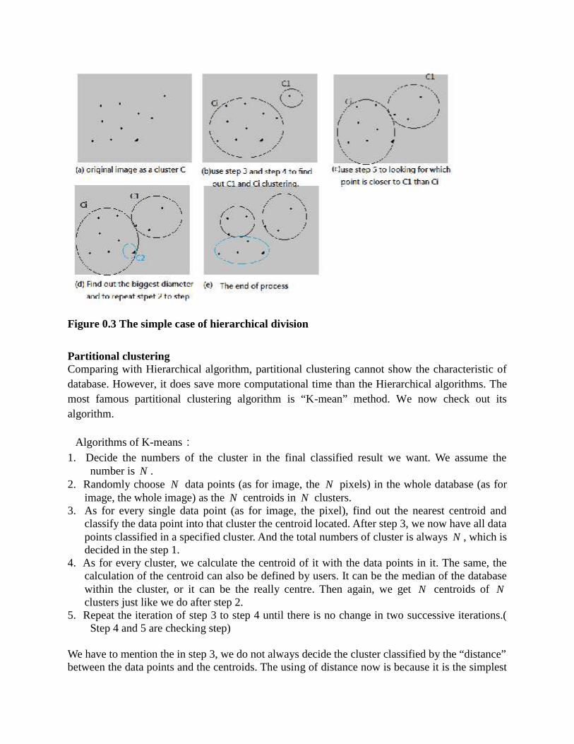
Figure 0.3 The simple case of hierarchical division
Partitional clusteringComparing with Hierarchical algorithm, partitional clustering cannot show the characteristic ofdatabase. However, it does save more computational time than the Hierarchical algorithms. Themost famous partitional clustering algorithm is “K-mean” method. We now check out itsalgorithm.
Algorithms of K-means:1. Decide the numbers of the cluster in the final classified result we want. We assume the
number is N .2. Randomly choose N data points (as for image, the N pixels) in the whole database (as for
image, the whole image) as the N centroids in N clusters.3. As for every single data point (as for image, the pixel), find out the nearest centroid and
classify the data point into that cluster the centroid located. After step 3, we now have all datapoints classified in a specified cluster. And the total numbers of cluster is always N , which isdecided in the step 1.
4. As for every cluster, we calculate the centroid of it with the data points in it. The same, thecalculation of the centroid can also be defined by users. It can be the median of the databasewithin the cluster, or it can be the really centre. Then again, we get N centroids of Nclusters just like we do after step 2.
5. Repeat the iteration of step 3 to step 4 until there is no change in two successive iterations.(Step 4 and 5 are checking step)
We have to mention the in step 3, we do not always decide the cluster classified by the “distance”between the data points and the centroids. The using of distance now is because it is the simplest
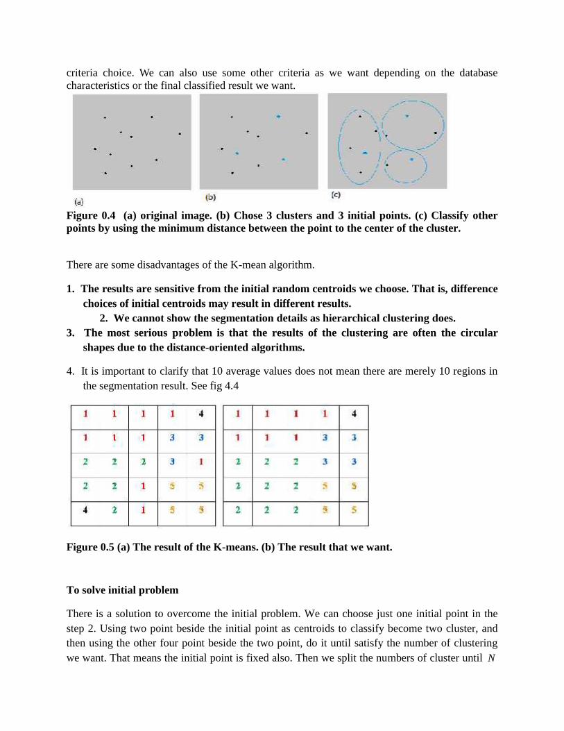
criteria choice. We can also use some other criteria as we want depending on the databasecharacteristics or the final classified result we want.
Figure 0.4 (a) original image. (b) Chose 3 clusters and 3 initial points. (c) Classify otherpoints by using the minimum distance between the point to the center of the cluster.
There are some disadvantages of the K-mean algorithm.
1. The results are sensitive from the initial random centroids we choose. That is, differencechoices of initial centroids may result in different results.
2. We cannot show the segmentation details as hierarchical clustering does.3. The most serious problem is that the results of the clustering are often the circular
shapes due to the distance-oriented algorithms.
4. It is important to clarify that 10 average values does not mean there are merely 10 regions inthe segmentation result. See fig 4.4
Figure 0.5 (a) The result of the K-means. (b) The result that we want.
To solve initial problem
There is a solution to overcome the initial problem. We can choose just one initial point in thestep 2. Using two point beside the initial point as centroids to classify become two cluster, andthen using the other four point beside the two point, do it until satisfy the number of clusteringwe want. That means the initial point is fixed also. Then we split the numbers of cluster until N
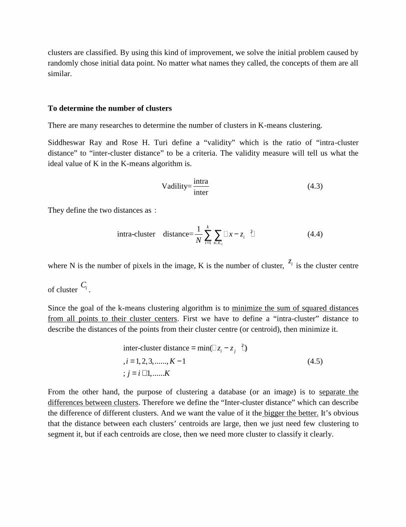
clusters are classified. By using this kind of improvement, we solve the initial problem caused byrandomly chose initial data point. No matter what names they called, the concepts of them are allsimilar.
To determine the number of clusters
There are many researches to determine the number of clusters in K-means clustering.
Siddheswar Ray and Rose H. Turi define a “validity” which is the ratio of “intra-clusterdistance” to “inter-cluster distance” to be a criteria. The validity measure will tell us what theideal value of K in the K-means algorithm is.
intraVadility=
inter(4.3)
They define the two distances as:
2
1
1intra-cluster distance=
i
k
ii x C
x zN
(4.4)
where N is the number of pixels in the image, K is the number of cluster, izis the cluster centre
of cluster iC.
Since the goal of the k-means clustering algorithm is to minimize the sum of squared distancesfrom all points to their cluster centers. First we have to define a “intra-cluster” distance todescribe the distances of the points from their cluster centre (or centroid), then minimize it.
2inter-cluster distance min( )
, 1,2,3,......, 1
; 1,......
i jz z
i K
j i K
(4.5)
From the other hand, the purpose of clustering a database (or an image) is to separate thedifferences between clusters. Therefore we define the “Inter-cluster distance” which can describethe difference of different clusters. And we want the value of it the bigger the better. It’s obviousthat the distance between each clusters’ centroids are large, then we just need few clustering tosegment it, but if each centroids are close, then we need more cluster to classify it clearly.
More method to solve initial problem but do not change the scheme of K-meanParticle Swarm optimization
PSO is a population-based randomly searching process. We assume that there are N“particles” randomly appear in a “solution space”. Mention that we are solving the optimizationproblem and for data clustering, there is always a criteria (for example, the squared errorfunction) for every single particle at their position in the solution space. The N particles willkeep moving and calculating the criteria in every position the stay (we call “fitness” in PSO)until the criteria reaches some threshold we need.
Each particle keeps track of its coordinates in the solution space which are associated with thebest solution (fitness) that has achieved so far by that particle. This value is called personal best,pbest.
Another best value that is tracked by the PSO is the best value obtained so far by any particle inthe neighborhood of that particle. This value is called global best, gbest.
We introduce the exact statement in mathematics below:
, , 1 1 ,
, 2 2 ,
,
( ) ( 1) ( ( 1)
( 1)) ( ( 1)
( 1))
i j i j i j
i j g j
i j
v t w v t c r p t
x t c r p t
x t
(4.6)
, , ,( ) ( 1) ( )i j i j i jx t x t v t (4.7)
where ix is the current position of the particle, iv is the current velocity of the particle, ip is the
personal best position of the particle, w, c, are all constant factors, and r are the random numbersuniform distributed within the interval [0,1].
We use last velocity and last position of personal and global best to predicate the velocity now.The position we stay is predicated by last position plus velocity now.
By using PSO, we can solve the initial problem of “K-means” and still maintain the wholepartitional clustering scheme. The most important thing is to think about it as an optimizationproblem.

Advantage and disadvantage of data clusteringHierarchical algorithm Partitional algorithms(K-means)
advantage 1. Concept is simple.2. Result is reliable. Result shows
strong correlation with originalimage.
3. Instead of calculating thecentroids of clusters, we haveto calculate the distancesbetween every single datapoint.
1. Computing speed is fast.2. Numbers of cluster is fixed, so
the concept is also simple.
disadvantage 1. Computing time isconsuming. So that thisalgorithm is not suitable forperforming on a largedatabase.
1. Numbers of cluster isfixed. So, what numbersof clustering we choose isthe best?
2. Initial problem.3. Partitional clustering
cannot show thecharacteristic of databasecompared withHierarchical clustering.
4. The results of theclustering are probably thecircular shapes.
5. We can’t improve K-means by setting lesscentroids.
We can solve the choice of numbers of clustering by observing the value “validity” proposed bySiddheswar Ray and Rose H. Turi. For the initial problem, we can solve it by choosing only oneinitial point or using the PSO algorithm directly.However, we cannot solve the circular shapes problem because that is due to the core computingscheme of partitional algorithms.
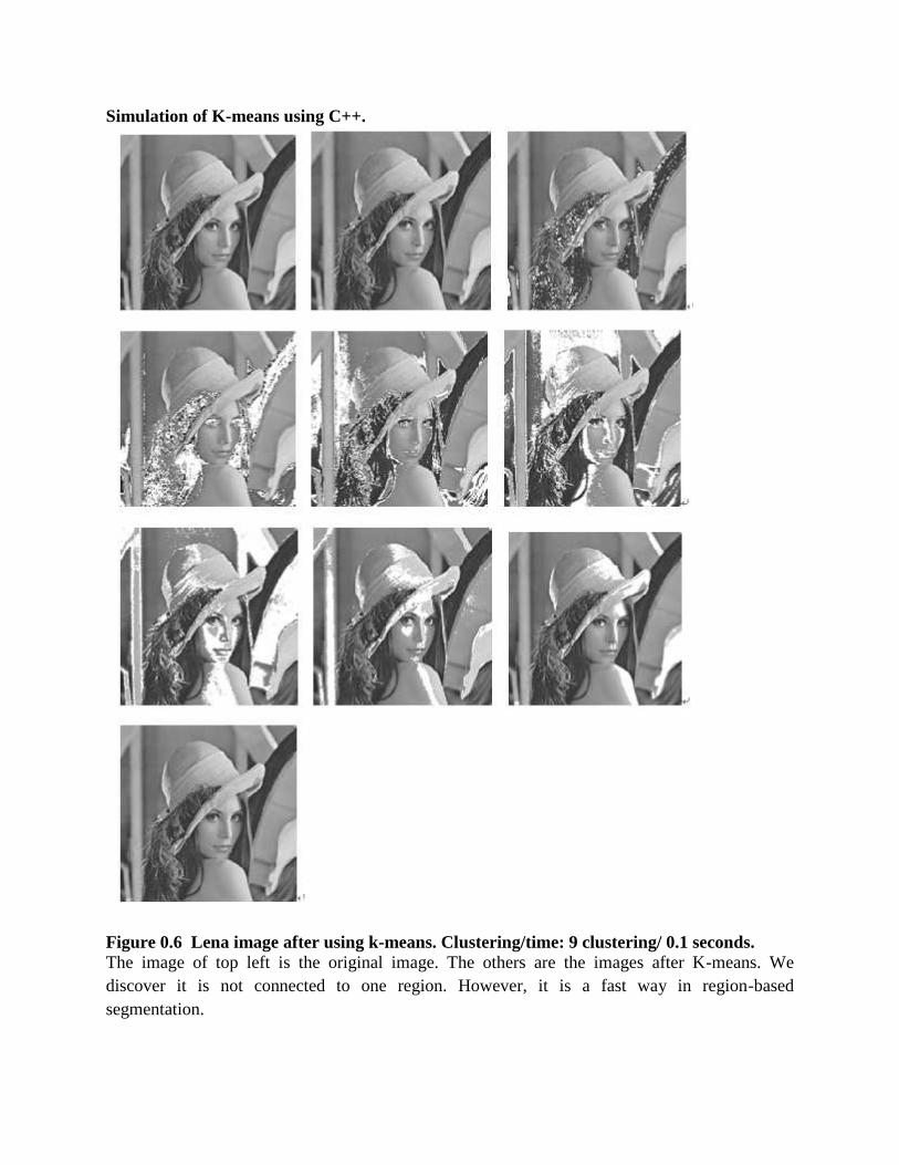
Simulation of K-means using C++.
Figure 0.6 Lena image after using k-means. Clustering/time: 9 clustering/ 0.1 seconds.The image of top left is the original image. The others are the images after K-means. Wediscover it is not connected to one region. However, it is a fast way in region-basedsegmentation.

Cheng-Jin Kuo`s methodWe will introduce the method we propose and explain why we would like to use this kind ofalgorithm by the “data compression”.
Ideal thought of segment we would like to obtain.The ideal result we would like to obtain is something like fig.5-6. It is very important for us toclassify the similar region together.
Figure 0.7 The ideal segment result we want.
We would like to see that the whole hair section is classified as one cluster. Because after weobtain the result, we can send the result directly to the compression stage to do the compressionfor every region. For almost all the methods of segmentation, it is unavoidable to over-segment aregion like the hair region in Lena image.
Algorithm of Cheng-Jin Kuo`s methodMake the first pixel (Mostly, it will be the top-left one) we scan as the first clustering.
1. See the pixel (x,1) in the image as one cluster iC . See the pixel which we are scanning as
jC .
2. From the first column, scan the next pixel (x,1+1) and make a decision with thethreshold if it will be merged into the first clustering or to be a new clustering.
If ( )j iC centroid C threshold , we merge jC into iC and recount the centroid of iC .
If ( )j iC centroid C threshold , we make jC as a new cluster 1iC .
3. Repeat step 2 until all the pixels in the same column have been scanned.

4. Scan the next column with pixel (x+1,1) and compare it to the region uC which is in the
upper side of it. And make the merge decision see if we have to merge pixel (x+1,1) tothe region uC .
If ( ) ,j uC centroid C threshold , we merge jC into uC and recount the centroid of uC .
If ( )j uC centroid C threshold , we make jC as a new cluster
, where n is the cluster number so farnC .
5. Scan the next pixel (x+1,1+1) and compare it to the region uC , lC which is upper to it
and in the left side of it, respectively. And make the merge decision see if we have tomerge pixel (x+1,1) to anyone of them.
If ( )j uC centroid C threshold and ( )j lC centroid C threshold ,
(1) We merge jC into uC , merge jC into lC .
(2) Combine the region uC and lC to be region nC , where n is the cluster number so
far.
(3) Recount the centroid of uC .
else if ( )j uC centroid C threshold and ( )j lC centroid C threshold ,
(1) We merge jC into uC and recount the centroid of uC .
else if ( )j uC centroid C threshold and ( )j lC centroid C threshold ,
(2) We merge jC into lC and recount the centroid of lC .else We make jC as a new
cluster , where n is the cluster number so farnC .
6. Repeat step 4 ~ step 5 until all the pixel in the image has been scanned.
7. Process the small regions which are classified from step1~ step4
It is important for us to deal with the isolated small regions carefully. For that we do not wantthere are too many fragmentary results after we segment the image using our method. Therefore,our goal is to classify the isolated small regions into the big region which is already classifiedand is adjacent to these isolated small regions.The following is the method to merge small region to big region.(a) We aim and are prepare to process the regions iR which have the small size.(For the
256x256 input images, we aim the regions which have the size below 32 pixels)
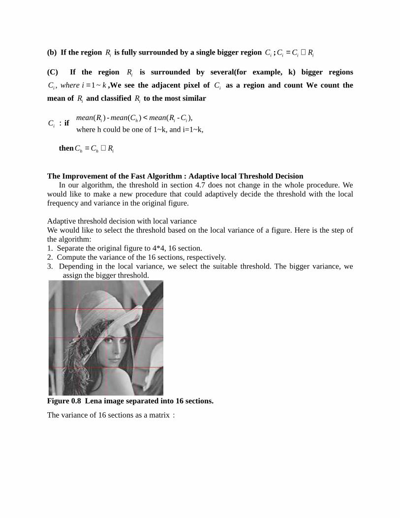
(b) If the region iR is fully surrounded by a single bigger region iC ; i i iC C R
(C) If the region iR is surrounded by several(for example, k) bigger regions
, 1 ~iC where i k ,We see the adjacent pixel of iC as a region and count We count the
mean of iR and classified iR to the most similar
iC :if( ) - ( ) ( - ),
where h could be one of 1~k, and i=1~k,i h i imean R mean C mean R C
then h h iC C R
The Improvement of the Fast Algorithm : Adaptive local Threshold DecisionIn our algorithm, the threshold in section 4.7 does not change in the whole procedure. We
would like to make a new procedure that could adaptively decide the threshold with the localfrequency and variance in the original figure.
Adaptive threshold decision with local varianceWe would like to select the threshold based on the local variance of a figure. Here is the step ofthe algorithm:1. Separate the original figure to 4*4, 16 section.2. Compute the variance of the 16 sections, respectively.3. Depending in the local variance, we select the suitable threshold. The bigger variance, we
assign the bigger threshold.
Figure 0.8 Lena image separated into 16 sections.
The variance of 16 sections as a matrix:
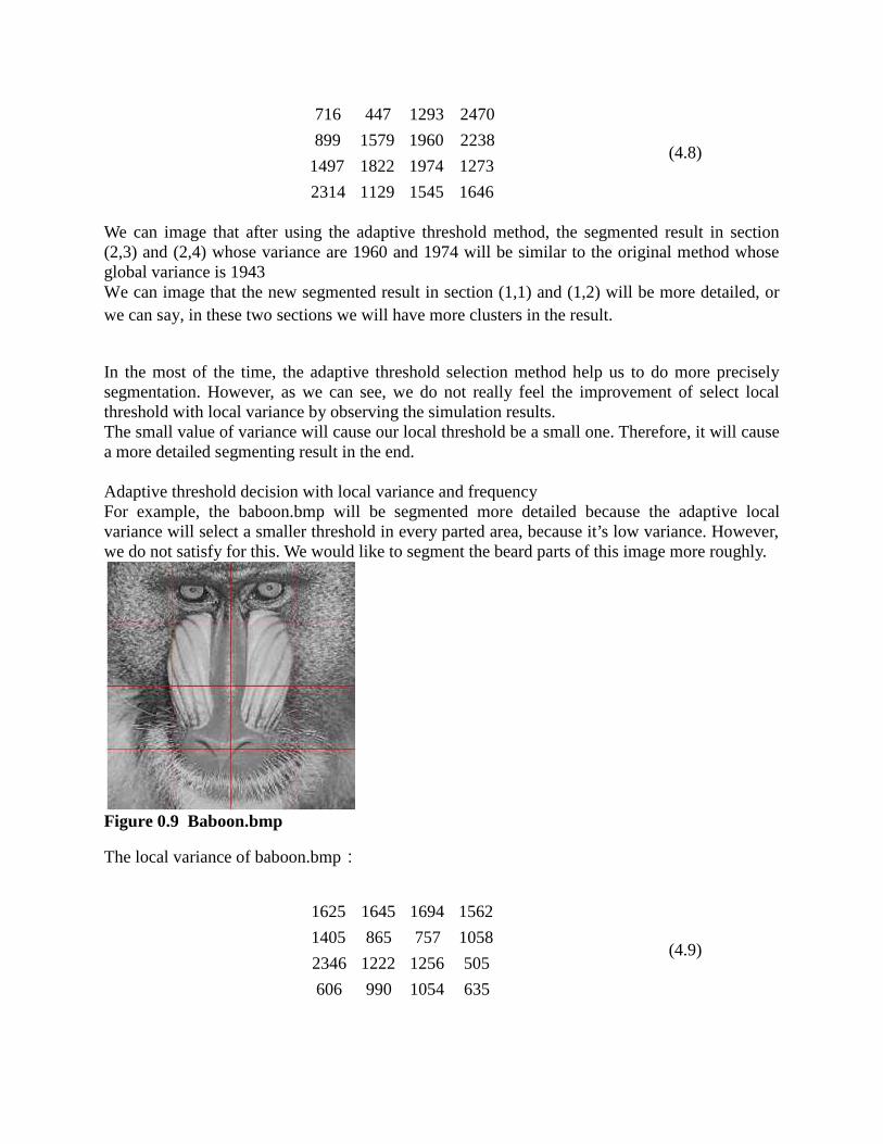
716 447 1293 2470
899 1579 1960 2238
1497 1822 1974 1273
2314 1129 1545 1646
(4.8)
We can image that after using the adaptive threshold method, the segmented result in section(2,3) and (2,4) whose variance are 1960 and 1974 will be similar to the original method whoseglobal variance is 1943We can image that the new segmented result in section (1,1) and (1,2) will be more detailed, orwe can say, in these two sections we will have more clusters in the result.
In the most of the time, the adaptive threshold selection method help us to do more preciselysegmentation. However, as we can see, we do not really feel the improvement of select localthreshold with local variance by observing the simulation results.The small value of variance will cause our local threshold be a small one. Therefore, it will causea more detailed segmenting result in the end.
Adaptive threshold decision with local variance and frequencyFor example, the baboon.bmp will be segmented more detailed because the adaptive localvariance will select a smaller threshold in every parted area, because it’s low variance. However,we do not satisfy for this. We would like to segment the beard parts of this image more roughly.
Figure 0.9 Baboon.bmp
The local variance of baboon.bmp:
1625 1645 1694 1562
1405 865 757 1058
2346 1222 1256 505
606 990 1054 635
(4.9)
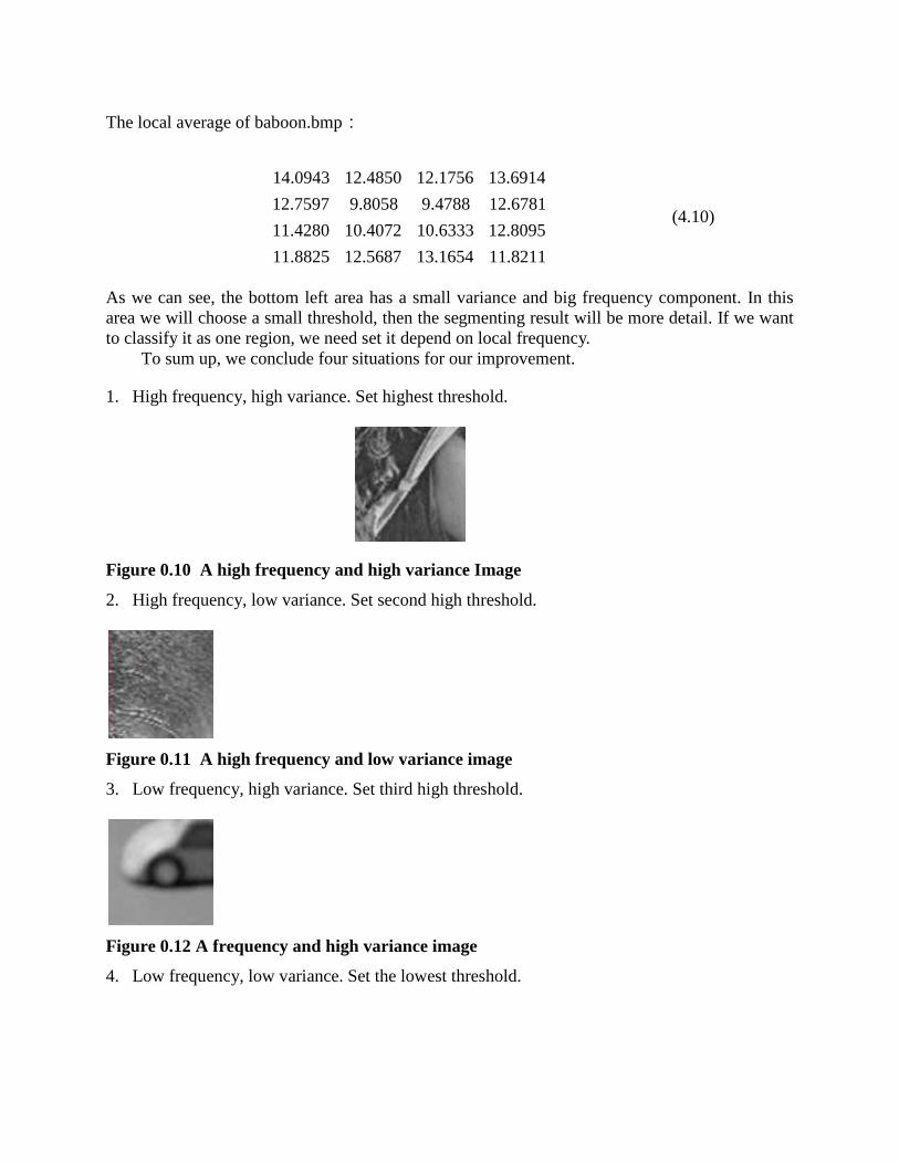
The local average of baboon.bmp:
14.0943 12.4850 12.1756 13.6914
12.7597 9.8058 9.4788 12.6781
11.4280 10.4072 10.6333 12.8095
11.8825 12.5687 13.1654 11.8211
(4.10)
As we can see, the bottom left area has a small variance and big frequency component. In thisarea we will choose a small threshold, then the segmenting result will be more detail. If we wantto classify it as one region, we need set it depend on local frequency.
To sum up, we conclude four situations for our improvement.
1. High frequency, high variance. Set highest threshold.
Figure 0.10 A high frequency and high variance Image
2. High frequency, low variance. Set second high threshold.
Figure 0.11 A high frequency and low variance image
3. Low frequency, high variance. Set third high threshold.
Figure 0.12 A frequency and high variance image
4. Low frequency, low variance. Set the lowest threshold.

Figure 0.13 A low frequency and low variance image
For the first case, the reason for a higher threshold we select is that there are often many edgesand different objects in this kind of area. The larger value of threshold may cause a roughsegmenting result, but we believe the clear edge and the high variety between different objectswill make the segmenting work. The larger threshold will remove some over-segmentation causeby the high variance and high frequency. It might be thought that the smallest threshold in casefour will cause an over-segment result. However, the stable and monotonous characteristic incase four will not make the over-segmentation work.
Decide the local threshold.we use a formula to decide the threshold:
16threshold F V (4.11)
The formula of F:
(local average frequency)F A B (4.12)
The formula of V:
(local variance)V C D (4.13)
In this thesis we always try to control the threshold value between 16 and 32 for the besttesting threshold value with the original method (without using adaptive threshold) will be 24.For that, the range of F will be 0 to 8, and so does the range of V. The maximum of F and V areall 8 which will make the maximum of threshold be 32.
If local average frequency>9,
F=6;
Else if local average frequency<3,
F=0;
End
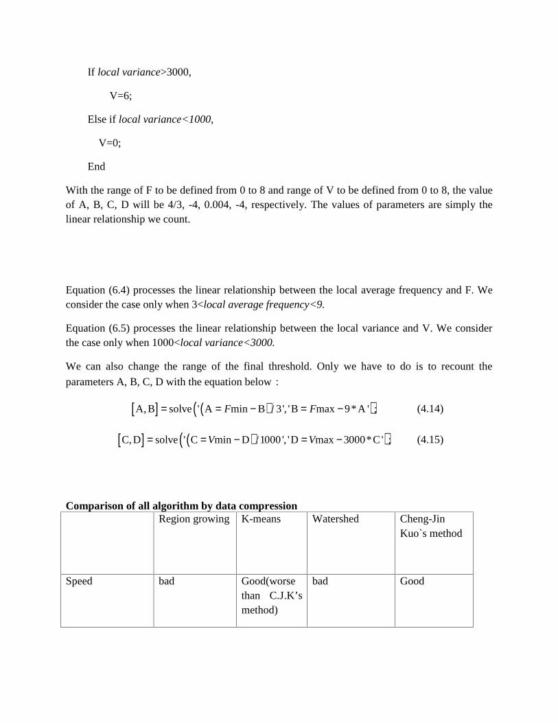
If local variance>3000,
V=6;
Else if local variance<1000,
V=0;
End
With the range of F to be defined from 0 to 8 and range of V to be defined from 0 to 8, the valueof A, B, C, D will be 4/3, -4, 0.004, -4, respectively. The values of parameters are simply thelinear relationship we count.
Equation (6.4) processes the linear relationship between the local average frequency and F. Weconsider the case only when 3<local average frequency<9.
Equation (6.5) processes the linear relationship between the local variance and V. We considerthe case only when 1000<local variance<3000.
We can also change the range of the final threshold. Only we have to do is to recount the
parameters A, B, C, D with the equation below:
A, B solve ' A min B / 3', 'B max 9*A ' ;F F (4.14)
C, D solve ' C min D /1000 ', 'D max 3000*C ' ;V V (4.15)
Comparison of all algorithm by data compressionRegion growing K-means Watershed Cheng-Jin
Kuo`s method
Speed bad Good(worsethan C.J.K’smethod)
bad Good
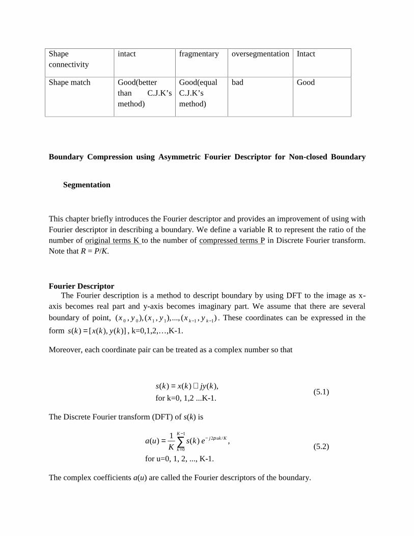
Shapeconnectivity
intact fragmentary oversegmentation Intact
Shape match Good(betterthan C.J.K’smethod)
Good(equalC.J.K’smethod)
bad Good
Boundary Compression using Asymmetric Fourier Descriptor for Non-closed Boundary
Segmentation
This chapter briefly introduces the Fourier descriptor and provides an improvement of using withFourier descriptor in describing a boundary. We define a variable R to represent the ratio of thenumber of original terms K to the number of compressed terms P in Discrete Fourier transform.Note that R = P/K.
Fourier DescriptorThe Fourier description is a method to descript boundary by using DFT to the image as x-
axis becomes real part and y-axis becomes imaginary part. We assume that there are several
boundary of point, 0 0 1 1 1 1( , ), ( , ),..., ( , )k kx y x y x y . These coordinates can be expressed in the
form ( ) [ ( ), ( )]s k x k y k , k=0,1,2,…,K-1.
Moreover, each coordinate pair can be treated as a complex number so that
( ) ( ) ( ),
for k=0, 1,2 ...K-1.
s k x k jy k (5.1)
The Discrete Fourier transform (DFT) of s(k) is
12 /
0
1( ) ( ) ,
for u=0, 1, 2, ..., K-1.
Kj uk K
k
a u s k eK
(5.2)
The complex coefficients a(u) are called the Fourier descriptors of the boundary.
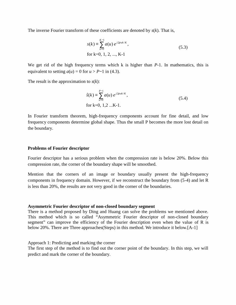
The inverse Fourier transform of these coefficients are denoted by s(k). That is,
12 /
0
( ) ( ) ,
for k=0, 1, 2, ..., K-1
Kj uk K
u
s k a u e
(5.3)
We get rid of the high frequency terms which k is higher than P-1. In mathematics, this is
equivalent to setting a(u) = 0 for u > P1 in (4.3).
The result is the approximation to s(k):
12 /
0
ˆ( ) ( ) ,
for k=0, 1,2 ...K-1.
Pj uk K
u
s k a u e
(5.4)
In Fourier transform theorem, high-frequency components account for fine detail, and lowfrequency components determine global shape. Thus the small P becomes the more lost detail onthe boundary.
Problems of Fourier descriptor
Fourier descriptor has a serious problem when the compression rate is below 20%. Below thiscompression rate, the corner of the boundary shape will be smoothed.
Mention that the corners of an image or boundary usually present the high-frequencycomponents in frequency domain. However, if we reconstruct the boundary from (5-4) and let Ris less than 20%, the results are not very good in the corner of the boundaries.
Asymmetric Fourier descriptor of non-closed boundary segmentThere is a method proposed by Ding and Huang can solve the problems we mentioned above.This method which is so called “Asymmetric Fourier descriptor of non-closed boundarysegment” can improve the efficiency of the Fourier description even when the value of R isbelow 20%. There are Three approaches(Steps) in this method. We introduce it below.[A-1]
Approach 1: Predicting and marking the cornerThe first step of the method is to find out the corner point of the boundary. In this step, we willpredict and mark the corner of the boundary.
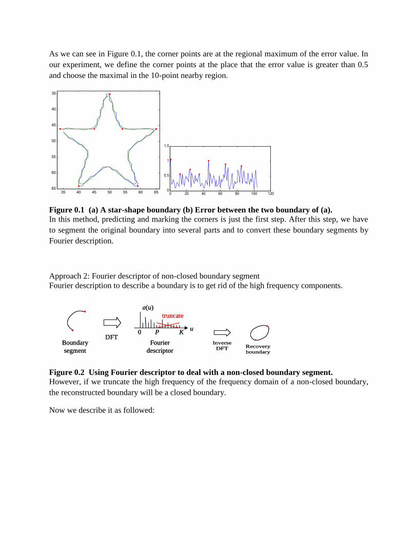
As we can see in Figure 0.1, the corner points are at the regional maximum of the error value. Inour experiment, we define the corner points at the place that the error value is greater than 0.5and choose the maximal in the 10-point nearby region.
Figure 0.1 (a) A star-shape boundary (b) Error between the two boundary of (a).In this method, predicting and marking the corners is just the first step. After this step, we haveto segment the original boundary into several parts and to convert these boundary segments byFourier description.
Approach 2: Fourier descriptor of non-closed boundary segmentFourier description to describe a boundary is to get rid of the high frequency components.
Figure 0.2 Using Fourier descriptor to deal with a non-closed boundary segment.However, if we truncate the high frequency of the frequency domain of a non-closed boundary,the reconstructed boundary will be a closed boundary.
Now we describe it as followed:
35 40 45 50 55 60 65
35
40
45
50
55
60
650 20 40 60 80 100 1200
0.5
1
1.5
u
a(u)
0
Boundarysegment
Fourierdescriptor
Recoveryboundary
truncate
P KDFT Inverse
DFT
Fig. . Use Fourier descriptor to a non-close boundary segment.
u
a(u)
0
Boundarysegment
Fourierdescriptor
Recoveryboundary
truncate
P KDFT Inverse
DFT
Fig. . Use Fourier descriptor to a non-close boundary segment.
u
a(u)
0
Boundarysegment
Fourierdescriptor
Recoveryboundary
truncate
P KDFT Inverse
DFT
Fig. . Use Fourier descriptor to a non-close boundary segment.
u
a(u)
0
Boundarysegment
Fourierdescriptor
Recoveryboundary
truncate
P KDFT Inverse
DFT
Fig. . Use Fourier descriptor to a non-close boundary segment.
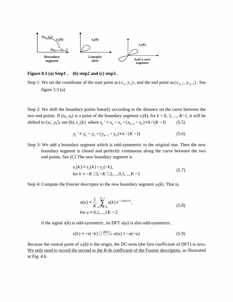
Figure 0.3 (a) Step1、 (b) step2 and (c) step3 .
Step 1: We set the coordinate of the start point as 0 0( , )x y , and the end point as 1 1( , )K Kx y . See
figure 5.3 (a)
Step 2: We shift the boundary points linearly according to the distance on the curve between thetwo end points. If (xk, yk) is a point of the boundary segment s1(k), for k = 0, 1, ..., K1, it will be
shifted to (xk', yk'), see (b), 2( )s k where 0 1 0' ( ) / ( 1)k k Kx x x x x k K (5.5)
0 1 0' ( ) / ( 1)k k Ky y y y y k K (5.6)
Step 3: We add a boundary segment which is odd-symmetric to the original one. Then the newboundary segment is closed and perfectly continuous along the curve between the twoend points. See (C) The new boundary segment is
3 2 2( ) ( ) ( ),
for 1, 2,...,0,1,..., 1
s k s k s k
k K K K
(5.7)
Step 4: Compute the Fourier descriptor to the new boundary segment s3(k). That is,
12 /
1
1( ) ( ) ,
for 0,1,..., 2 2
Kj uk K
k K
a u s k eK
u K
(5.8)
if the signal s(k) is odd-symmetric, its DFT a(u) is also odd-symmetric.
( ) ( ) ( ) ( )DFTs k s k a u a u (5.9)
Because the central point of s3(k) is the origin, the DC-term (the first coefficient of DFT) is zero.We only need to record the second to the K-th coefficient of the Fourier descriptors, as illustratedin Fig. 4.6.
s1(k) s2(k) s3(k)
Boundarysegment
Linearlyshift
Add a newsegment
Fig. . The steps to solve the non-closed problem.
(x0, y0)
(xK1, yK1)
s1(k) s2(k) s3(k)
Boundarysegment
Linearlyshift
Add a newsegment
Fig. . The steps to solve the non-closed problem.
(x0, y0)
(xK1, yK1)
s1(k) s2(k) s3(k)
Boundarysegment
Linearlyshift
Add a newsegment
Fig. . The steps to solve the non-closed problem.
(x0, y0)
(xK1, yK1)
s1(k) s2(k) s3(k)
Boundarysegment
Linearlyshift
Add a newsegment
Fig. . The steps to solve the non-closed problem.
(x0, y0)
(xK1, yK1)

Figure 0.4 Fourier descriptor of 3s
After doing all the steps, we can start to take the Fourier description of the processed boundaryand the problem we mention will not exist anymore.
Approach 3: Boundary compressionThis is talk about the process in approach 2 which can use on boundary compression.
We can only reserve the P1 coefficients and truncate the other coefficients. We recover thewhole coefficient by stuffing zeroes and then copy to the odd symmetry part
Figure 0.5 The reserve P1 coefficients
Figure 0.6 Recover the whole coefficients from fig. 5.5
Approach 4: boundary encodingIn the boundary segments encoding, we have four data to record:
u
|a(u)|
0
useless
K 2K2
s3
DFT
odd symmetry
DC-term is zero
u
|a(u)|
0
useless
K 2K2
s3
DFT
odd symmetry
DC-term is zerou
|a(u)|
0
useless
K 2K2
s3
DFT
odd symmetry
DC-term is zero
u
|a(u)|
0
useless
K 2K2
s3
DFT
odd symmetry
DC-term is zero
u
|a(u)|
0 K1P1
only reserve P1coefficients |a(u)|
P1
odd symmetrytruncate
u0 2K2
u
|a(u)|
0 K1P1
only reserve P1coefficients |a(u)|
P1
odd symmetrytruncate
u0 2K2
u
|a(u)|
0 K1P1
only reserve P1coefficients |a(u)|
P1
odd symmetrytruncate
u0 2K2
u
|a(u)|
0 K1P1
only reserve P1coefficients |a(u)|
P1
odd symmetrytruncate
u0 2K2
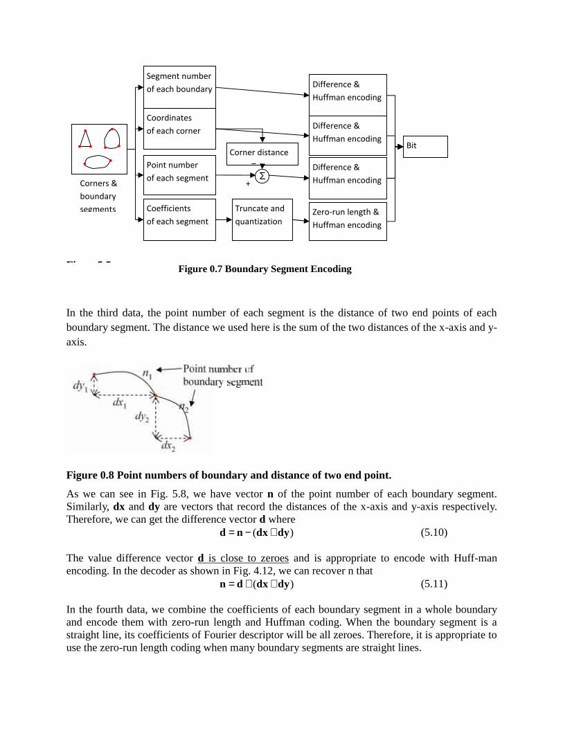
Figure5.5
In the third data, the point number of each segment is the distance of two end points of eachboundary segment. The distance we used here is the sum of the two distances of the x-axis and y-axis.
Figure 0.8 Point numbers of boundary and distance of two end point.
As we can see in Fig. 5.8, we have vector n of the point number of each boundary segment.Similarly, dx and dy are vectors that record the distances of the x-axis and y-axis respectively.Therefore, we can get the difference vector d where
( ) d n dx dy (5.10)
The value difference vector d is close to zeroes and is appropriate to encode with Huff-manencoding. In the decoder as shown in Fig. 4.12, we can recover n that
( ) n d dx dy (5.11)
In the fourth data, we combine the coefficients of each boundary segment in a whole boundaryand encode them with zero-run length and Huffman coding. When the boundary segment is astraight line, its coefficients of Fourier descriptor will be all zeroes. Therefore, it is appropriate touse the zero-run length coding when many boundary segments are straight lines.
Coordinatesof each corner
Coefficientsof each segment
Segment numberof each boundary
Point numberof each segment
Truncate andquantization
Corner distance
Zero-run length &Huffman encoding
Difference &Huffman encoding
Difference &Huffman encoding
Difference &Huffman encoding
+
Bitstream
Corners &boundarysegments
Figure 0.7 Boundary Segment EncodingFigure5.5
In the third data, the point number of each segment is the distance of two end points of eachboundary segment. The distance we used here is the sum of the two distances of the x-axis and y-axis.
Figure 0.8 Point numbers of boundary and distance of two end point.
As we can see in Fig. 5.8, we have vector n of the point number of each boundary segment.Similarly, dx and dy are vectors that record the distances of the x-axis and y-axis respectively.Therefore, we can get the difference vector d where
( ) d n dx dy (5.10)
The value difference vector d is close to zeroes and is appropriate to encode with Huff-manencoding. In the decoder as shown in Fig. 4.12, we can recover n that
( ) n d dx dy (5.11)
In the fourth data, we combine the coefficients of each boundary segment in a whole boundaryand encode them with zero-run length and Huffman coding. When the boundary segment is astraight line, its coefficients of Fourier descriptor will be all zeroes. Therefore, it is appropriate touse the zero-run length coding when many boundary segments are straight lines.
Coordinatesof each corner
Coefficientsof each segment
Segment numberof each boundary
Point numberof each segment
Truncate andquantization
Corner distance
Zero-run length &Huffman encoding
Difference &Huffman encoding
Difference &Huffman encoding
Difference &Huffman encoding
+
Bitstream
Corners &boundarysegments
Figure 0.7 Boundary Segment Encoding
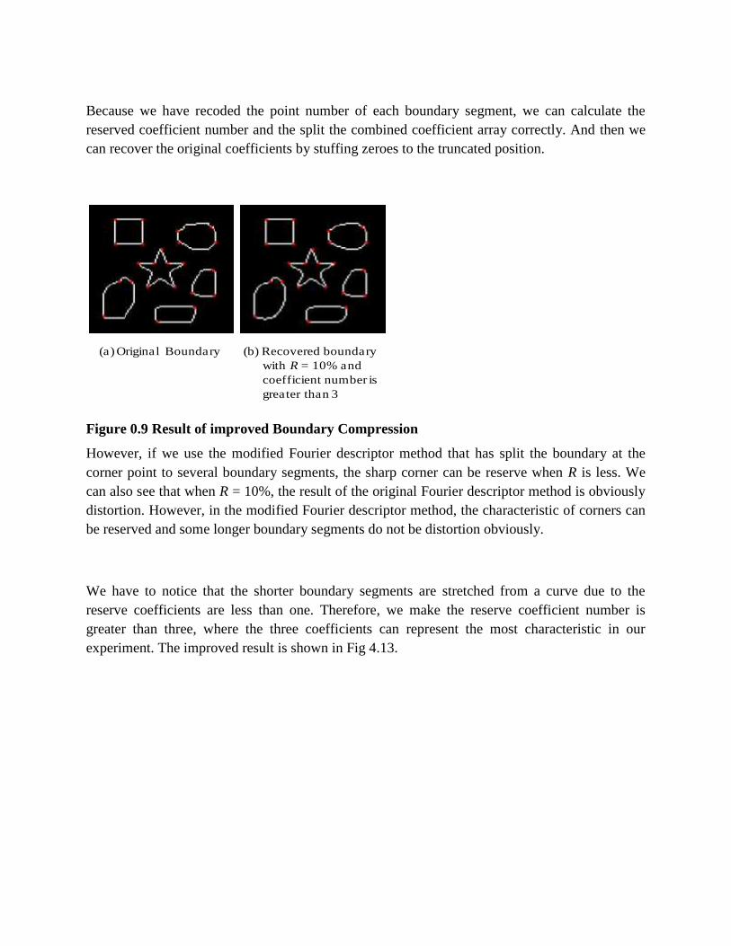
Because we have recoded the point number of each boundary segment, we can calculate thereserved coefficient number and the split the combined coefficient array correctly. And then wecan recover the original coefficients by stuffing zeroes to the truncated position.
Figure 0.9 Result of improved Boundary Compression
However, if we use the modified Fourier descriptor method that has split the boundary at thecorner point to several boundary segments, the sharp corner can be reserve when R is less. Wecan also see that when R = 10%, the result of the original Fourier descriptor method is obviouslydistortion. However, in the modified Fourier descriptor method, the characteristic of corners canbe reserved and some longer boundary segments do not be distortion obviously.
We have to notice that the shorter boundary segments are stretched from a curve due to thereserve coefficients are less than one. Therefore, we make the reserve coefficient number isgreater than three, where the three coefficients can represent the most characteristic in ourexperiment. The improved result is shown in Fig 4.13.
(a) Original Boundary (b) Recovered boundarywith R = 10% andcoefficient number isgreater than 3
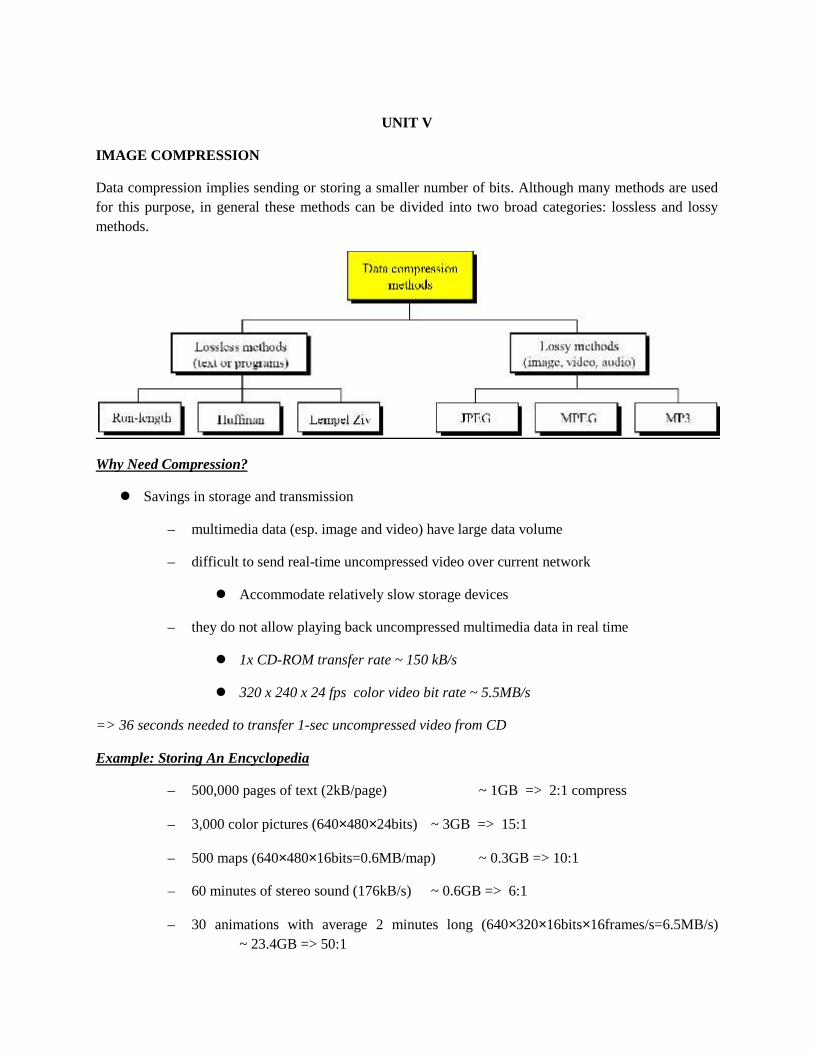
UNIT V
IMAGE COMPRESSION
Data compression implies sending or storing a smaller number of bits. Although many methods are usedfor this purpose, in general these methods can be divided into two broad categories: lossless and lossymethods.
Why Need Compression?
Savings in storage and transmission
– multimedia data (esp. image and video) have large data volume
– difficult to send real-time uncompressed video over current network
Accommodate relatively slow storage devices
– they do not allow playing back uncompressed multimedia data in real time
1x CD-ROM transfer rate ~ 150 kB/s
320 x 240 x 24 fps color video bit rate ~ 5.5MB/s
=> 36 seconds needed to transfer 1-sec uncompressed video from CD
Example: Storing An Encyclopedia
– 500,000 pages of text (2kB/page) ~ 1GB => 2:1 compress
– 3,000 color pictures (64048024bits) ~ 3GB => 15:1
– 500 maps (64048016bits=0.6MB/map) ~ 0.3GB => 10:1
– 60 minutes of stereo sound (176kB/s) ~ 0.6GB => 6:1
– 30 animations with average 2 minutes long (64032016bits16frames/s=6.5MB/s)~ 23.4GB => 50:1

– 50 digitized movies with average 1 minute long (64048024bits30frames/s =27.6MB/s) ~ 82.8GB => 50:1
– Require a total of 111.1GB storage capacity if without compression
– Reduce to 2.96GB if with compression
Outline
Lossless encoding tools
– Entropy coding: Huffman, Lemple-Ziv, and others (Arithmetic coding)
– Run-length coding
Lossy tools for reducing redundancy
– Quantization and truncations
Predictive coding
Transform coding
– Zonal coding (truncation)
– Rate-distortion and bit allocation
– Tree structure
Vector quantization
Huffman Coding
Variable length code
– assigning about log2 (1 / pi) bits for the ith value
has to be integer# of bits per symbol
Step-1
– Arrange pi in decreasing order and consider them as tree leaves
Step-2
– Merge two nodes with smallest probabilities to a new node and sum up probabilities
– Arbitrarily assign 1 and 0 to each pair of merging branch
Step-3
– Repeat until no more than one node left.
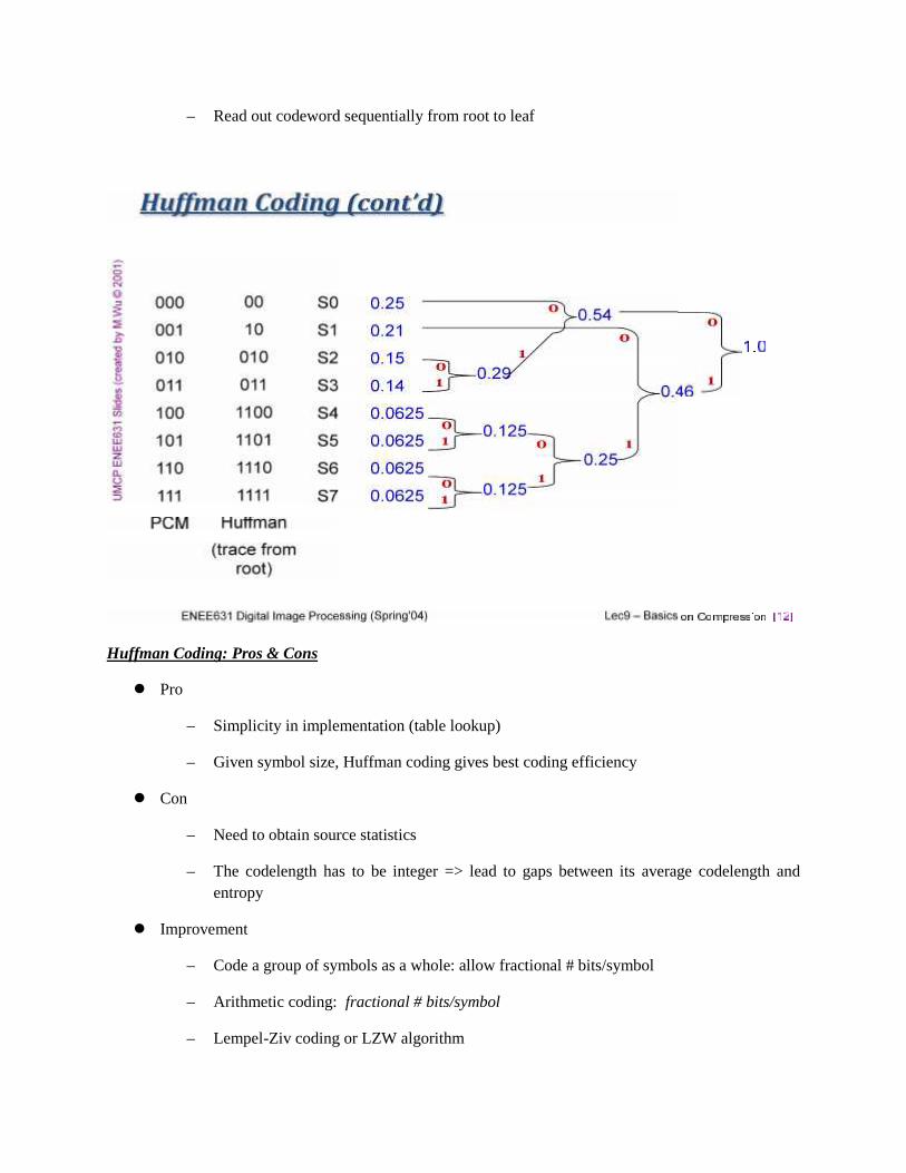
– Read out codeword sequentially from root to leaf
Huffman Coding: Pros & Cons
Pro
– Simplicity in implementation (table lookup)
– Given symbol size, Huffman coding gives best coding efficiency
Con
– Need to obtain source statistics
– The codelength has to be integer => lead to gaps between its average codelength andentropy
Improvement
– Code a group of symbols as a whole: allow fractional # bits/symbol
– Arithmetic coding: fractional # bits/symbol
– Lempel-Ziv coding or LZW algorithm
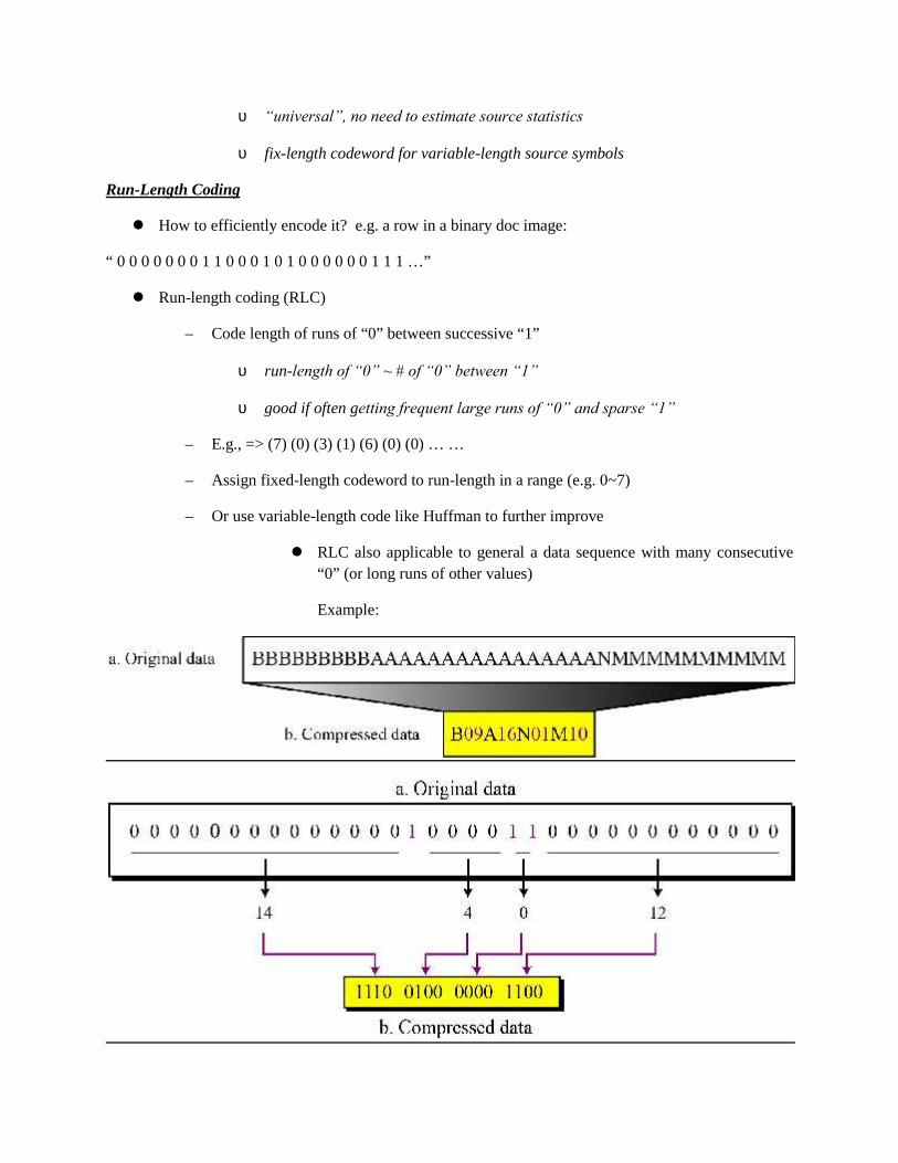
“universal”, no need to estimate source statistics
fix-length codeword for variable-length source symbols
Run-Length Coding
How to efficiently encode it? e.g. a row in a binary doc image:
“ 0 0 0 0 0 0 0 1 1 0 0 0 1 0 1 0 0 0 0 0 0 1 1 1 …”
Run-length coding (RLC)
– Code length of runs of “0” between successive “1”
run-length of “0” ~ # of “0” between “1”
good if often getting frequent large runs of “0” and sparse “1”
– E.g., => (7) (0) (3) (1) (6) (0) (0) … …
– Assign fixed-length codeword to run-length in a range (e.g. 0~7)
– Or use variable-length code like Huffman to further improve
RLC also applicable to general a data sequence with many consecutive“0” (or long runs of other values)
Example:
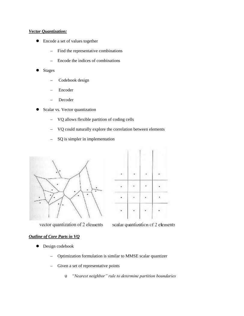
Vector Quantization:
Encode a set of values together
– Find the representative combinations
– Encode the indices of combinations
Stages
– Codebook design
– Encoder
– Decoder
Scalar vs. Vector quantization
– VQ allows flexible partition of coding cells
– VQ could naturally explore the correlation between elements
– SQ is simpler in implementation
Outline of Core Parts in VQ
Design codebook
– Optimization formulation is similar to MMSE scalar quantizer
– Given a set of representative points
“Nearest neighbor” rule to determine partition boundaries
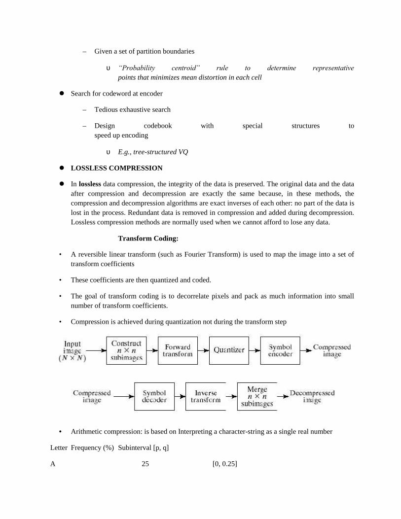
– Given a set of partition boundaries
“Probability centroid” rule to determine representativepoints that minimizes mean distortion in each cell
Search for codeword at encoder
– Tedious exhaustive search
– Design codebook with special structures tospeed up encoding
E.g., tree-structured VQ
LOSSLESS COMPRESSION
In lossless data compression, the integrity of the data is preserved. The original data and the dataafter compression and decompression are exactly the same because, in these methods, thecompression and decompression algorithms are exact inverses of each other: no part of the data islost in the process. Redundant data is removed in compression and added during decompression.Lossless compression methods are normally used when we cannot afford to lose any data.
Transform Coding:
• A reversible linear transform (such as Fourier Transform) is used to map the image into a set oftransform coefficients
• These coefficients are then quantized and coded.
• The goal of transform coding is to decorrelate pixels and pack as much information into smallnumber of transform coefficients.
• Compression is achieved during quantization not during the transform step
• Arithmetic compression: is based on Interpreting a character-string as a single real number
Letter Frequency (%) Subinterval [p, q]
A 25 [0, 0.25]

B 15 [0.25, 0.40]
C 10 [0.40, 0.50]
D 20 ?
E 30 ?
• Arithmetic compression: Coding ‘CABAC’
• Generate subintervals of decreasing length, subintervals depend uniquely on the string’scharacters and their frequencies.
• Interval [x, y] has width w = y – x, the new interval based on [p, q] is x = x + w.p, y = x + w.q
• Step 1: ‘C’ 0………..0.4…….0.5…………..1
based on p = 0.4, q = 0.5
• Step 2: ‘A’ 0.4………0.425..…….…………..0.5
based on p = 0.0, q = 0.25
• Step 3: ‘B’ 0.4……0.40625………0.41…..……0.425
based on p = 0.25, q = 0.4
Step 4: ‘A’
Step 5: ‘C’
…0.406625… 0.4067187…
Final representation (midpoint)?
• Arithmetic compression: Extracting ‘CABAC’
N Interval[p, q] Width Character N-p (N-p)/width
0.40670.4 – 0.5 0.1 C 0.0067 0.067
0.067 0 – 0.25 0.25 A 0.067 0.268
0.268 0.25 – 0.4 0.15 B 0.018 0.12
?
?
When to stop? A terminal character is added to the original
character set and encoded. During decompression, once it is

encountered the process stops.
JPEG:
• JPEG compression – both for grayscale and color images
• Previous compression methods were lossless – it was possible to recover all the information fromthe compressed code
• JPEG is lossy: image recovered may not be the same as the original
• It consists of three phases: Discrete Cosine Transform (DCT), Quantization, Encoding.
• DCT:
Image is divided into blocks of 8*8 pixels
For grey-scale images, pixel is represented by 8-bits
For color images, pixel is represented by 24-bits or three 8-bit groups
• DCT takes an 8*8 matrix and produces another 8*8 matrix.
• T[i][j] = 0.25 C(i) C(j) ∑ ∑ P[x][y] Cos (2x+1)iπ/16 * Cos (2y+1)jπ/16
i = 0, 1, …7, j = 0, 1, …7
C(i) = 1/√2, i =0
= 1 otherwise
T contains values called ‘Spatial frequencies’
• Spatial frequencies directly relate to how much the pixel values change as a function of theirpositions in the block
• T[0][0] is called the DC coefficient, related to average values in the array/matrix, Cos 0 = 1
• Other values of T are called AC coefficients, cosine functions of higher frequencies
• Case 1: all P’s are same => image of single color with no variation at all, AC coefficients are allzeros.
• Case 2: little variation in P’s => many, not all, AC coefficients are zeros.
• Case 3: large variation in P’s => a few AC coefficients are zeros.
P-matrix T-matrix
• 20 30 40 50 60 … 720 -182 0 -19 0 …
30 40 50 60 70 -182 0 0 0 0

40 50 60 70 80 0 0 0 0 0
50 60 70 80 90 -19 0 0 0 0
60 70 80 90 1000 0 0 0 0
… …
‘Uniform color change and little fine detail, easier to compress after DCT’
P-matrix T-matrix
• 100 150 50 100 100 … 835 15 -17 59 5…
200 10 110 20 200 46 -60 -36 11 14
10 200 130 30 200 -32 -9 130 105 -37
100 10 90 190 120 59 -3 27 -12 30
10 200 200 120 90 50 -71 -24 -56 -40
…. ….
‘Large color change, difficult to compress after DCT ’
• To restore, inverse DCT (IDCT) is performed:
• P[x][y] = 0.25 ∑ ∑ C(i) C(j) T[i][j] Cos (2x+1)iπ/16 * Cos (2y+1)jπ/16
x = 0, 1, …7, y = 0, 1, …7
# Can write a C-program to apply DCT on a P-array (8*8) to obtain T-array and also IDCT on T-array torecover P-array.
• Quantization: Provides an way of ignoring small differences in an image that may not beperceptible.
• Another array Q is obtained by dividing each element of T by some number and rounding-off tonearest integer => loss