Fast Mesh Segmentation using Random Walks

Yu-Kun Lai∗

Tsinghua UniversityBeiing, China

Shi-Min Hu†

Tsinghua UniversityBeijing, China

Ralph R. Martin‡

Cardiff UniversityWales, UK

Paul L. Rosin§

Cardiff UniversityWales, UK

Abstract

3D mesh models are now widely available for use in various appli-cations. The demand for automatic model analysis and understand-ing is ever increasing. Mesh segmentation is an important step to-wards model understanding, and acts as a useful tool for differentmesh processing applications, e.g. reverse engineering and model-ing by example. We extend a random walk method used previouslyfor image segmentation to give algorithms for both interactive andautomatic mesh segmentation. This method is extremely efficient,and scales almost linearly with increasing number of faces. Formodels of moderate size, interactive performance is achieved withcommodity PCs. It is easy-to-implement, robust to noise in themesh, and yields results suitable for downstream applications forboth graphical and engineering models.

CR Categories: I.3.5 [Computational Geometry and Object Mod-eling]: Geometric algorithms, languages, and systems.

Keywords: mesh segmentation, random walks, interactive

1 Introduction

With the development of 3D acquisition techniques, 3D mesh mod-els are now widely available and used in various applications. Thedemand for model analysis and understanding is thus ever increas-ing. However, techniques for intelligent automated processing oflarge mesh models have not matched the growth in availability ofmodels. The task of mesh segmentation is to decompose a meshmodel into a set of disjoint pieces whose union corresponds to theoriginal model. To be useful, segmentation must decompose a meshinto meaningful pieces (e.g. limbs and torso of an animal) or oneswhich satisfy other desirable criteria (e.g. each piece is bounded bysharp edges or small radius blends).

Mesh segmentation is an important step towards model analysisand understanding. A variety of different applications could benefitfrom preprocessing the mesh using an efficient and reliable meshsegmentation method. In the field of reverse engineering of CADmodels, segmentation plays an important role in splitting a modelinto pieces, each of which may then be fitted with a single analyt-ical surface [Varady et al. 1997]. In computer graphics, segmen-tation can be applied in various applications, including mesh sim-plification [Zuckerberger et al. 2002], collision detection [Li et al.2001], morphing [Shlafman et al. 2002; Zuckerberger et al. 2002]and skeleton-driven animation [Katz and Tal 2003].

∗e-mail:laiyk03@mails.thu.edu.cn†e-mail:shimin@tsinghua.edu.cn‡e-mail:ralph@cs.cf.ac.uk§e-mail:Paul.Rosin@cs.cf.ac.uk

The basis for mesh segmentation derives from cognitive science.As pointed out by Hoffmann [Hoffmann and Richards 1984; Hoff-mann and Singh 1997], the human visual system perceives regionboundaries at negative minima of principal curvature, or concavecreases—this observation is known as the minima rule. The depthof the concavity directly affects the salience of region boundaries.Such concave feature regions together with other information areimportant cues for segmentation. Moreover, it can be observed thatonly significant features are important to segmentation; small-scalefluctuations should be ignored, even if they represent sharp creases.On the other hand, in the case of reverse engineering, different sur-faces are separated along sharp edges, which may be convex or con-cave, or even along smooth edges—different criteria are applicableto segmentation for such uses.

Recently, Grady [2006] proposed an interactive algorithm for imagesegmentation based on the use of random walks. The main ideasare as follows: a set of seed pixels is first specified by the user. Forall other pixels, using an efficient process, we determine the prob-ability that a random walk starting at that pixel first reaches eachparticular seed, given some definition of the probability of steppingfrom a given pixel to each neighbor. The segmentation is formed byassigning the label of the seed first reached to the non-seed pixel.

Our work is an extension of the random walks method to the partic-ular problem of mesh segmentation; previous work has already con-sidered the use of random walks for solving the different problemof mesh denoising [Sun et al. 2007]. By using different methodsof assigning probability distributions, we are able to segment bothengineering object models and graphical models. Our results are re-liable even when the models are noisy or have small-scale texturesthat should be ignored.

As well as a method based on user selection of seeds, we give a gen-eralization of this method to automatic mesh segmentation, whichautomatically places seeds (usually with more seeds than the re-quired number of regions) using feature sensitive isotropic pointsampling. Our two-pass method segments the mesh using these ini-tial seeds, and then merges the regions found based on similaritiesof neighboring regions.

Compared to other methods, our proposed method has the follow-ing advantages. Our method:

• provides results of comparable quality to state-of-the-artmethods, but is significantly more efficient, making it espe-cially suitable for interactive applications or applications thatrequire segmentation of large models, or large numbers ofmodels,

• can be used both interactively or automatically, and in partic-ular the optimal number of regions can be deduced automati-cally,

• is robust to noise and small-scale texture that may be presentin real scanned models,

• is applicable to both CAD models and graphical models, and

• is easy-to-implement.

Section 2 briefly reviews related work. Interactive and automaticmesh segmentation algorithms based on random walks are pre-

sented in Sections 3 and 4 respectively. Experimental results aregiven in Section 5, with conclusions and discussions in Section 6.

2 Related Work

Compared to the problem of image segmentation, research intomesh segmentation is much more recent; however, it is now an ac-tive research topic, due to the wide range of potential applications.A complete survey of mesh segmentation is beyond the scope of thepaper, but an up-to-date review and comparison of different meth-ods can be found in [Attene et al. 2006a].

Based on the different aims, existing mesh segmentation algorithmscan be generally categorized into two classes. The first class isaimed at applications such as reverse engineering of CAD models(e.g. [Attene et al. 2006b]). Such methods segment a mesh modelinto patches each of which is a best fit to one of a given class ofmathematical surfaces, e.g. planes, cylinders, etc. The second classtries to segment typically ‘natural objects’ into meaningful pieces,as expected by a human observer. Our algorithm is mainly aimed atsolving problems of the latter class, but with certain modifications,it is also able to handle engineering objects reasonably well.

Most state-of-the-art work on mesh segmentation is based on it-erative clustering. Shlafman et al. [2002] use k-means clusteringto segment the models into meaningful pieces. Katz [Katz andTal 2003] improved on this by using fuzzy clustering and minimalboundary cuts to achieve smoother boundaries between clusters.Top-down hierarchical segmentation has also been used to segmentobjects with a natural hierarchy of features. Lai [Lai et al. 2006]suggested combining integral and statistical quantities derived fromlocal surface characteristics, producing more meaningful results onmeshes with noise or repeated patterns. One of the most prominentdrawbacks of such algorithms is the necessity to compute pairwisedistances, making it expensive or even prohibitive to handle largemodels directly. To handle models with e.g. more than 10,000faces, mesh simplification [Katz and Tal 2003; Katz et al. 2005;Liu and Zhang 2004] or remeshing [Lai et al. 2006] is typicallyused. Spectral clustering has also been used [Liu and Zhang 2004]with good results, but this approach also suffers from performanceproblems, although Nystrom approximation method has been usedfor accelerating it [Liu et al. 2006].

Unsupervised clustering techniques like the mean shift method canalso be applied to mesh segmentation. Shamir [Shamir et al. 2004]extended mean shift analysis to mesh models based on use of alocal parameterization method. Later, Yamauchi [Yamachi et al.2005] applied mean shift clustering to surface normals. Such meth-ods tend to oversegment a model into more pieces than expected ordesired.

Other methods for mesh segmentation also exist. Mangan andWhitaker [1999] applied bobsledding watershed algorithm to tri-angle meshes. Li [Li et al. 2001] proposed using skeletonizationbased on edge contraction and space sweeping to perform meshdecomposition. Visually appealing results are obtained; however,their results depend mainly on large-scale features, and do not al-ways capture salient geometric features. Recently, Reniers andTelea [2007] used curve skeletons in hierarchical mesh segmenta-tion. Katz [Katz et al. 2005] proposed a segmentation algorithmbased on multidimensional scaling and extraction of feature pointsand cores. The method is able to produce consistent results whenregions of a mesh are placed in differing relative poses. However,an expensive method is used to find feature points, which limitsthe complexity of models that can be efficiently handled, even aftersimplification. Mitani [Mitani and Suzuki 2004] proposed a tech-

nique for making paper models from meshes. This can be consid-ered to be a specialized mesh segmentation method that producesnaturally developable triangle strips.

In the sense of segmentation of engineering objects, especially forthe purpose of reverse engineering, there exist quite a few works.Most of such work deals with point cloud directly instead of tri-angle meshes due to its wide availability. Sapidis and Besl [Sa-pidis and Besl 1995] proposed a method to construct polynomialsurfaces from point cloud data, using region growing for segmen-tation. Benko and Varady [2002] proposed a method to directlysegment point cloud data of engineering objects based on a serialof top-down recursive tests. Gelfand and Guibas [2004] proposedto use slippage analysis and multi-pass region growing to segmentdifferent regions based on different slippage signatures. Edels-brunner [Edelsbrunner et al. 2003] proposed to segment mesheswith piecewise linear Morse-Smale theory. This idea has been ex-tended to suit the needs for producing CAD-like segmentation re-sults [Varady 2007].

Certain work explicitly considers the problem of interactive meshsegmentation. Lee proposed a method to segment models us-ing user-guided or automatically extracted cut lines based on 3Dsnakes [Lee et al. 2004; Lee et al. 2005]. Funkhouser [Funkhouseret al. 2004] provided an intuitive interactive segmentation tool tofind optimal cuts guided by user-drawn strokes, and applied it to amodeling system based on stitching parts extracted from a modeldatabase. An interactive segmentation method based on graph-cut was proposed by Sharf, again for use in a cut-and-paste sys-tem [Sharf et al. 2006].

Our method is different to any of the above in that it is based on arandom walk paradigm. The formulation leads to the need to solvea sparse linear system, which is very efficient. Unlike most interac-tive methods, user interaction is provided by specifying a set of seedmesh faces, which is much easier than specifying a rough cuttingboundary. In applications where automatic methods are preferred,we use a two-stage method that first oversegments the mesh usinga set of automatically chosen seeds, and then merges these initialregions to give the final regions.

3 Interactive Segmentation

In this section, we will discuss our algorithm for interactive meshsegmentation using random walks; extension to an automatic meshsegmentation algorithm will be discussed in the next section. Thebasic idea of the algorithm is in spirit similar to the correspondingmethod for image segmentation [Grady 2006], but due to the differ-ences of source data and aims, certain issues must be resolved.

We assume that the given models are triangular meshes. Randomwalk mesh segmentation proceeds as follows: assume that the userpicks n faces as seeds, where n is the number of final regionsdesired; seeds are placed so that one seed ‘obviously’ lies withineach of the final regions the user desires. We denote the seeds bys1, . . . , sn. Other faces are non-seed faces, denoted by f1, . . . , fm.We associate a probability with each of the three edges ek,i ofeach non-seed face fk, denoted by pk,1, pk,2 and pk,3 respectively.These correspond to the probabilities that a random walk will moveacross a particular edge to the corresponding neighbor. These prob-abilities satisfy the following equation:

3∑i=1

pk,i = 1. (1)

For i = 1, 2, 3, denote the face sharing ek,i with fk by fk,i. Fora particular seed face sl, denote the probability of a random walk

starting from a particular face fk arriving at sl first, before reachingother seeds, as P l(fk), for l = 1, . . . , n. P l(sl) = 1 and P l(sk) =0 for any k 6= l. As the number of steps considered increases, in thelimit, the following equation holds for each non-seed face fk (foreach l = 1, 2, . . . n):

P l(fk) =

3∑i=1

pk,iPl(fk,i). (2)

For a particular seed face sl, the P l(fk) form a column vector oflength m (denoted by P l) that needs to be computed, and we havem equations of the form given in Eqn. 2. We may rewrite Eqn. 2 inmatrix form as Am×mP l = Bl, where A and Bl can be deducedfrom Eqn. 2. Most values in Bl are zeros. However, from Eqn. 2,for a non-seed face fk adjacent to a seed face, the correspondingP l(fk,i) is not a variable, but a constant, either 0 (if not the lth

seed) or 1 (for lth seed). Since the lth seed has at most (and nor-mally, exactly) three neighbors, Bl also has at most (and normally)three non-zero values.

Note that A is independent of the choice of l. Thus we may put theP l together and form a matrix Pm×n with rows Pl,k = P l(fk),to give AP = B, where B = (B1, . . . , Bn). This sparse linearsystem has the same general nature as the one in [Grady 2006]; thissystem is sparse as each row of the matrix contains at most 4 non-zero entries, as shown in Eqn 2. Following the argument in [Grady2006], the matrix A is positive semi-definite, and the solution tothis linear system is uniquely determined. Please note that randomwalk model described above is in essence equivalent to electric net-work model as the distribution of electric potentials at each face,where the probability to move to neighboring face corresponds tothe reciprocal of resistors (i.e. conductances). See [Doyle and Snell1984] for a thorough study.

We now define that a given face belongs to the region attached toseed sl if a random walk starting at that face has a higher probabilityof reaching this seed than any other seed. Thus, after computingP l(fk) for l = 1, . . . , n and k = 1, 2, . . . , m, we assign the labelfor seed sl to those non-seed faces fk which satisfy

P l(fk) = maxt=1,...,n

P t(fk). (3)

It can be shown that each region produced by this segmentationprocess is guaranteed to be contiguous.

Given the basic framework given by the algorithm above, two sig-nificant issues remain: to determine appropriate probabilities forstepping from face to face, what optional preprocessing and post-processing steps may be needed to further improve the results.

3.1 Probability computation

Choice of suitable probability assignments, i.e. pi,1, pi,2, pi,3, foreach face i is essential for the random walk approach to give goodmesh segmentation results. Appropriate probabilities are affectedby the types of models, due to the different purposes of mesh seg-mentation. In the following, we will address ‘natural’ graphicalmodels and engineering object models separately.

3.1.1 Graphical models

Mesh segmentation of graphical models should split a model intomeaningful pieces. The most important information for segmenta-tion comes from the minima rule, as used by many segmentationalgorithms, where significant (concave) features are considered as

important hints. For a given face fi, we define a difference func-tion d(fi, fi,k) which measures the difference in some specific ge-ometric property between fi and one of its neighboring faces fi,k,k = 1, 2, 3. For graphical models, we define this function to mainlydepend on a function d1 measuring the dihedral angle:

d1(fi, fi,k) = η [1− cos (dihedral(fi, fi,k))] =η

2||Ni −Ni,k||2 ,

(4)where dihedral(fl, fm) represents the dihedral angle between ad-jacent faces fl and fm, and Nl is the normal to face fl. η is used togive higher priority to concave edges: we set η = 1.0 for concaveedges and a relatively small number (e.g. 0.2) for convex edges,according to the minima rule.

To handle variations in the dihedral distribution, we normalize d1

by its average over all edges, d1, giving as the overall differencefunction d:

d(fi, fi,k) =d1(fi, fi,k)

d1

. (5)

Given a definition for the difference function at hand, the probabil-ity distribution is now computed as

pi,k = |ei,k| exp

{−d(fi, fi,k)

σ

}, (6)

where |ei,k| is the edge length of the corresponding common edge,and σ is used to control how variation of differences maps to vari-ations in probability. In our experiments, we have found σ = 1.0works well for most of cases. pi,k is then normalized to sum to oneover each face. An exponential function is used above as a con-venient way of mapping differences in (0,∞) to probabilities in(0, 1), where a high difference corresponds to a low probability

3.1.2 Engineering models

Segmentation of engineering object meshes differs in its aims fromsegmentation of graphical models. We usually want to segmentsuch a mesh into pieces that can each be fitted with some analyt-ical surface [Varady et al. 1997]. In many typical cases (but notall), Gaussian and mean curvatures should be almost uniform overa segment, which is a different requirement from the case of graph-ical models.

Again, we use d1 to measure the change of normals between ad-jacent faces; however, for engineering object mesh segmentation,we set η = 1.0 for both convex and concave edges, since they areequally important for the segmentation of such models. Moreover,we introduce two further difference measures for the variation ofGaussian and mean curvatures. To begin with, we need to estimatethe Gaussian and mean curvatures on both sides of a given edge.Such curvature estimates are known to be sensitive to noise, so weuse robust estimators for this purpose—we use PCA-based integralinvariants in ball neighborhoods [Yang et al. 2006]. The methodbasically relies on a covariance analysis of the intersection volumebetween a ball of radius r and the volume of interior part of thegiven model. Since the method actually computes principal tensorsat a regular mesh point, we may adapt this method to directly in-terpolate the principal curvatures at the center of each face ratherthan at each vertex. We denote Gaussian and mean curvatures atface fi as K(fi) and H(fi) respectively. If the model is relativelyclean, we may set r to be 1 to 2 times the average edge length of themodel. For noisy models, to make the result robust, we must usea larger radius r at the cost of sacrificing the ability to accuratelylocate some boundaries.

The difference functions for Gaussian and mean curvatures are nowdefined as

d2(fi, fi,k) = |K(fi)−K(fi,k)|d3(fi, fi,k) = |H(fi)−H(fi,k)| . (7)

The overall difference function is defined by combining d1, d2 andd3 to be:

d∗(fi, fi,k) = max

{d1(fi, fi,k)

d1

,d2(fi, fi,k)

d2

,d3(fi, fi,k)

d3

},

(8)where d1, d2 and d3 are average values of the corresponding dif-ference function over the whole model. Note that the maximumof these three is used instead of their weighted average: the peakresponses of any component are significant, and this approach alsoavoids the difficulty of choosing appropriate weights. Given d∗, theprobability is again defined using Eqn. 6, but with d∗ in place of d.The method works well for separating smoothly touching regions,as illustrated in Fig. 1.

Figure 1: segmentation of CAD models without sharp edges.

3.2 Preprocessing and postprocessing

Although the method as described is much faster than any methodbased on iterative clustering, for very large models, it may bepreferable to simplify or remesh the models to a more practical size(e.g.10, 000-20, 000 faces) for efficiency. This is also reasonable,since extra detail in models actually provides little extra help insegmentation. Segmentation can be computed using the faces ofthe reduced model. This step is optional for the overall pipeline.

After random walk segmentation, each segment is represented by acontiguous set of faces. The boundaries may be somewhat jagged,partly due to noise and other variations in local properties nearthe separating edges, and partially due to the limited resolution ofthe mesh. We use feature sensitive smoothing as proposed in [Laiet al. 2007] to smooth the segment boundaries while keeping themsnapped to features. This amounts to optimizing a discretizedspline-in-tension energy in the feature sensitive metric. The bound-aries generally form a complicated graph, so branching points arefirst detected and each boundary segment between branching pointsis smoothed independently.

The smoothed boundaries are represented as a set of connectedpoints; however each point generally will not be located at anyvertex of the initial mesh. We suggest updating the input meshmodel slightly so that the smoothed boundaries map to a sequenceof edges in the updated mesh. To do so, we first project each pointon the smoothed boundary onto the input mesh model. The re-sulting point may be located at a vertex, on an edge, or within aface. In the latter two cases, we split the related faces to make this

point a vertex of the revised mesh (as illustrated in Fig. 2(left)).Projection is done quickly using the approximate nearest neigh-bors library [Mount and Arya 2005]. After projection, we findthe geodesic path across the mesh between adjacent projected ver-tices [Surazhsky et al. 2005], and split each face crossed by thegeodesic into two. To ensure that the resulting mesh remains a tri-angular mesh, quad faces induced by this splitting are further splitinto two triangles.

Such local updates can be performed efficiently. Since the geodesiccomputation requires a data structure that cannot be easily adaptedfor dynamic updating of the mesh structure, we use the assumptionthat adjacent points on the smoothed boundaries are usually closeto each other, build a small patch of the input mesh that covers bothprojected points, and compute the geodesics on such small patches.An example of such splitting is shown in Fig. 2(right). The blueedges correspond to those which must be added so that geodesicedges become edges of the mesh. Thick blue edges correspond toedges that are part of the smoothed boundary. After this process,the smoothed boundaries can be directly mapped to edges of themodified input model, and the segmentation results after smoothingmay be represented by assigning a label to each face of the modifiedinput mesh.

4 Automatic Segmentation

The random walk segmentation method may be adapted to workautomatically. In this case, a set of seeds is automatically selected,generally with more seeds than the number of finally expected clus-ters. For segmentation of graphical models, we usually require acoarse segmentation, which does not need a dense set of seeds; forengineering object meshes, or when a detailed segmentation is pre-ferred, more seeds may be necessary. Our interface allows users tospecify both an approximate number of seeds, and to place specificseeds before or after automatic selection.

The random walk algorithm described above is used to segment themodel. There will in general be more resulting pieces than desired,and so a further merging process is used to combine these overseg-mented pieces into the final segments. This approach works well inpractice, as it is based on our experimental observation that randomwalk segmentation results are not sensitive to the exact location ofthe seeds (as demonstrated later).

4.1 Coarse-Scale Seeding

If it is desired to segment the model into large pieces represent-ing large-scale structures, we should generally evenly distribute asparse set of seeds, so that only the most significant features orprotrusions are captured. Based on the observation that the seg-mentation results are generally insensitive to the exact location ofseeds, we use a clustering method similar to that used in k-meansclustering segmentation.

The first seed face is selected as the (or a) face furthest away, interms of geodesic distance, from the face closest to the centroidof all faces. We then iteratively add new seed faces one by one.For any two faces fi and fj , a path from fi to fj is a contiguoussequence of faces starting from fi and ending at fj . For any path,we may compute the sum of the difference measures d (or d∗ ifappropriate), and select the minimal sum among all possible paths,denoting it by D(fi, fj). Assume s1, . . . , sn are n faces alreadyselected as seeds. The next seed face sn+1 is determined by

sn+1 = arg maxfk∈F

{min

i=1,...,nD(fk, si)

}, (9)

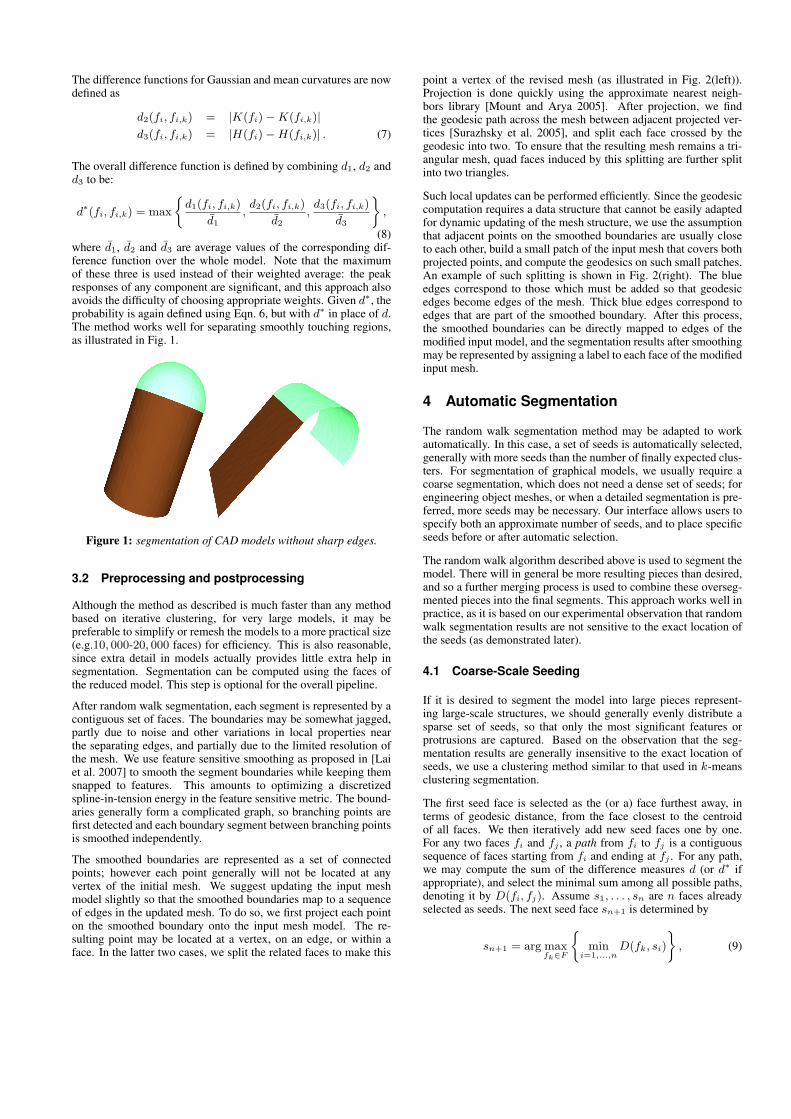
projected on face projected on edge

Figure 2: Projection and local update of the input model. Left: mapping smoothed boundary points onto the surface; right: mappingsmoothed boundary paths onto the surface.

Figure 3: Example of coarse seeding (left) and corresponding segmentation result (right).

where F is the set of all the faces. This process terminates whena significant decrease of D occurs between the newly selectedsn+1 to the nearest neighboring seed, whereupon sn+1 is dis-carded. Note that this computation is efficient, since we only needto solve a few single-source shortest distance problems startingfrom each seed face. Using Dijkstra’s algorithm gives a complexityof O(nm log m), where n and m are the number of seed faces andthe total number of faces, respectively.

Fig. 3 shows an example of coarse seeding. The left figure gives thepositions of seeds (the colored balls indicating the seed locations)and the right figure is the corresponding segmentation result.

4.2 Fine-Scale Seeding

In certain cases, we would like to segment the model into smallerpieces, where significant parts are segmented as much as possible.For example, given the skeleton example shown in Fig. 3, we maywant to segment to further detail than simply 5 fingers. Fine-scaleseeding based on automatic seed distribution and merging is thenmore appropriate.

4.2.1 Automatic seed selection

We should pick a set of random faces that are in general evenly dis-tributed over the surface, and gives higher priority to protrusionsand regions containing features. Feature sensitive sampling (thefirst phase of feature sensitive remeshing proposed in [Lai et al.2007]) suits this need well. The method basically distributes parti-cles over the model optimizing some spring-like energy [Witkin andHeckbert 1994]. After distribution, we pick those faces with parti-cles in them as seeds. For our purpose, we may use a sufficientlylarge number of sampling faces (e.g. 20–200 for most models).Again assuming that n is the number of seeds, and m is the total

number of faces, the time complexity is O(n log m), since nearestneighbor queries are performed using kd-tree acceleration. Place-ment of initial seeds is typically very fast (much less than a sec-ond). Note that if the original number of seeds is not large enoughto cover all the significant features, our semi-automatic interfaceallows users to add further seeds where desired.

4.2.2 Merging

Using such an approach, we expect many segments to have multi-ple seeds, which naturally leads to over-segmentation. However,as segmentation results are in general not sensitive to the exactplacement of seeds, we may simply merge the resulting segmentsto give suitable final regions. We perform merging as an iterativeprocess. To define the relative merging cost between two adjacentsegments Si and Sj , we first denote by ∂Si ∩ ∂Sj the commonboundary of the two segments, and by ∂Si ∪ ∂Sj the combinationof the two boundaries. We integrate the difference measure d (ord∗ if appropriate) along the common boundary, and denote it byD∂Si∩∂Sj =

∑e∈∂Si∩∂Sj

|e|de, where |e| and de are the lengthof edge e and the difference measure d (or d∗) between the twofaces adjacent to e. We also define the overall length of commonboundary as L∂Si∩∂Sj =

∑e∈Si∩Sj

|e|. D∂Si∪∂Sj and L∂Si∪∂Sj

can be defined similarly. We then define the relative merging costci,j as:

ci,j =D∂Si∩∂Sj /L∂Si∩∂Sj

D∂Si∪∂Sj /L∂Si∪∂Sj

. (10)

For each adjacent pair of segments Si and Sj , we compute themerging cost ci,j and put the pairs into a priority queue. Themerging process proceeds by picking the pair with minimal merg-ing cost, merging them into one segment and updating the prior-ity queue accordingly. This process can be terminated either when

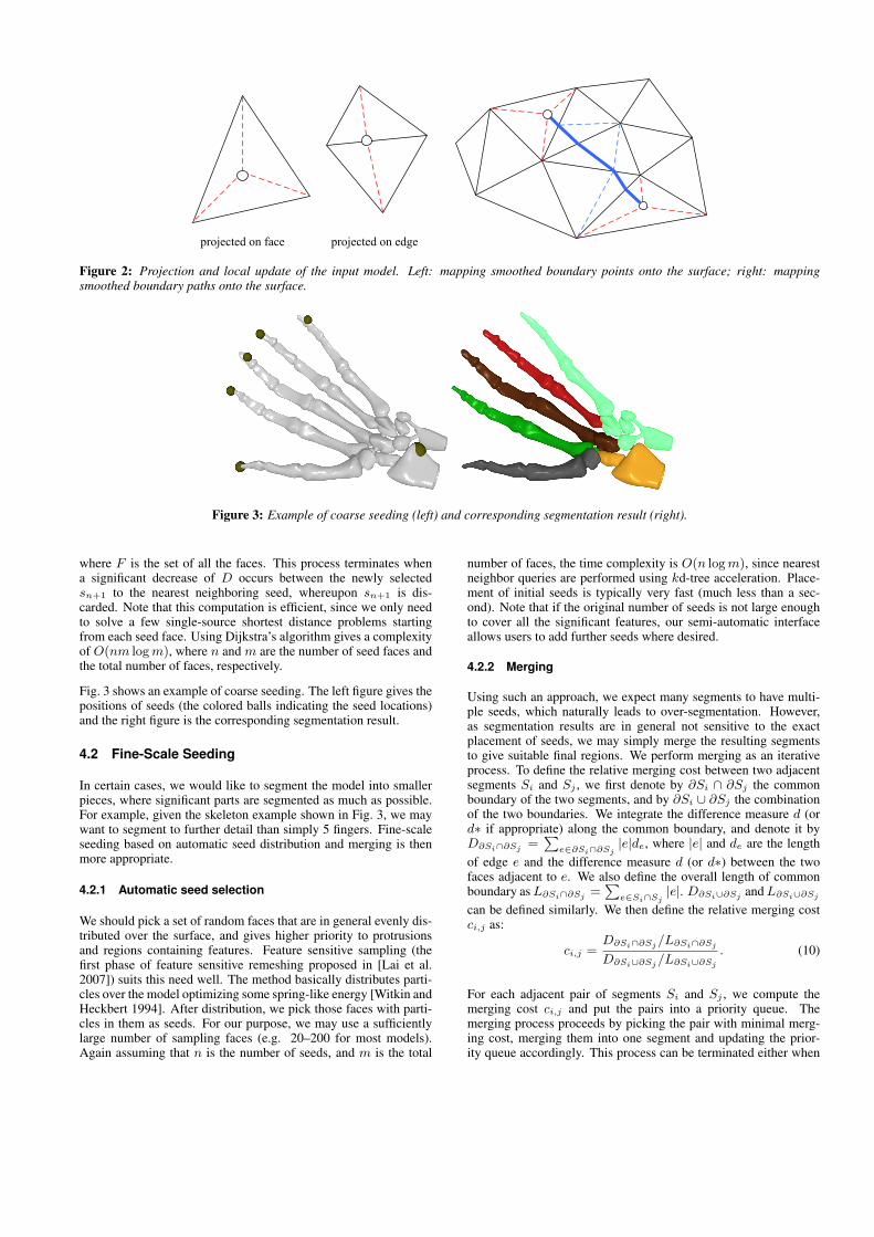
Figure 4: Example of fine-scale seeding. From top left to bottom right: input model with automatic seed selection; initial (over-) segmentedresults; result after merging; final result after boundary smoothing and mapping.

Figure 5: Segmentation of horse with varying seed locations. Balls represent seed locations.

there exists a significant increase in ci,j for the current pair, or whenwe have reached a final number of regions desired by the user. Inour experiments, the merging process usually stops with minimalrelative cost of about 0.5.

Experimental results of automatic segmentation before and aftermerging are shown in Fig. 4. The initial number of seeds is 60and the number of segments after merging is 30.

5 Experimental Results

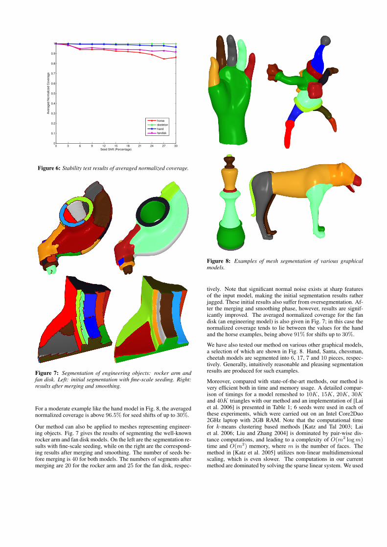
Our method is in general insensitive to the exact location of seeds.Fig. 5 shows an example of segmenting a horse model. Note thatthere are no clearly defined boundaries between the legs and thebody, so changing the positions of the seeds has a slight effect onthe final result; however, even if the seed positions are changedsignificantly, the results are similar, and snap to some local features.

A more accurate test of stability with respect to choice of seed faces

was also performed. Given some maximal seed shift radius r, weallow all seeds to move randomly to any face within a geodesic dis-tance of r from their original seed position (but we restrict new seedpositions to be within the same segment found by segmentation us-ing the original seeds). We performed tests using maximal shiftsof 3%, 6%, 9%, . . . , 30% of the size of the model. In each testwe computed the percentage of faces with the same labels foundwhen using the initial seeds (we call this the normalized coverage).To obtain a robust result, we performed 100 trials for each shiftdistance and averaged the normalized coverage. As illustrated inFig. 6, for models like the horse example in Fig. 5 where no clearlydefined boundaries exist between segments, the normalized cover-age decreases gradually with increasing shift. Even for shifts ofup to 30%, the averaged normalized coverage is above 84%. Formodels like the hand skeleton example in Fig. 3, where significantfeatures exist between segments, the averaged normalized coverageis above 99.6% for shifts up to 30%, which means almost identicalresults are produced even with significant change of seed locations.

0 3 6 9 12 15 18 21 24 27 300

0.1

0.2

0.3

0.4

0.5

0.6

0.7

0.8

0.9

1

Seed Shift (Percentage)

Ave

rag

ed

No

rma

lize

d C

ove

rag

e

horse

skeleton

hand

fandisk

Figure 6: Stability test results of averaged normalized coverage.

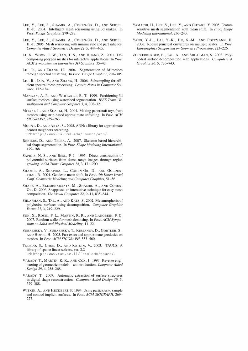
Figure 7: Segmentation of engineering objects: rocker arm andfan disk. Left: initial segmentation with fine-scale seeding. Right:results after merging and smoothing.

For a moderate example like the hand model in Fig. 8, the averagednormalized coverage is above 96.5% for seed shifts of up to 30%.

Our method can also be applied to meshes representing engineer-ing objects. Fig. 7 gives the results of segmenting the well-knownrocker arm and fan disk models. On the left are the segmentation re-sults with fine-scale seeding, while on the right are the correspond-ing results after merging and smoothing. The number of seeds be-fore merging is 40 for both models. The numbers of segments aftermerging are 20 for the rocker arm and 25 for the fan disk, respec-

Figure 8: Examples of mesh segmentation of various graphicalmodels.

tively. Note that significant normal noise exists at sharp featuresof the input model, making the initial segmentation results ratherjagged. These initial results also suffer from oversegmentation. Af-ter the merging and smoothing phase, however, results are signif-icantly improved. The averaged normalized coverage for the fandisk (an engineering model) is also given in Fig. 7; in this case thenormalized coverage tends to lie between the values for the handand the horse examples, being above 91% for shifts up to 30%.

We have also tested our method on various other graphical models,a selection of which are shown in Fig. 8. Hand, Santa, chessman,cheetah models are segmented into 6, 17, 7 and 10 pieces, respec-tively. Generally, intuitively reasonable and pleasing segmentationresults are produced for such examples.

Moreover, compared with state-of-the-art methods, our method isvery efficient both in time and memory usage. A detailed compar-ison of timings for a model remeshed to 10K, 15K, 20K, 30Kand 40K triangles with our method and an implementation of [Laiet al. 2006] is presented in Table 1; 6 seeds were used in each ofthese experiments, which were carried out on an Intel Core2Duo2GHz laptop with 2GB RAM. Note that the computational timefor k-means clustering based methods [Katz and Tal 2003; Laiet al. 2006; Liu and Zhang 2004] is dominated by pair-wise dis-tance computations, and leading to a complexity of O(m2 log m)time and O(m2) memory, where m is the number of faces. Themethod in [Katz et al. 2005] utilizes non-linear multidimensionalscaling, which is even slower. The computations in our currentmethod are dominated by solving the sparse linear system. We used

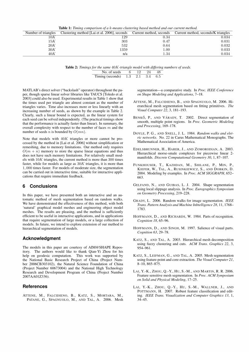
Table 1: Timing comparison of a k-means clustering based method and our current method.Number of triangles Clustering method [Lai et al. 2006], seconds Current method, seconds Current method, seconds/K triangles

10K 129 0.34 0.03415K 303 0.47 0.03120K 532 0.64 0.03230K 1359 1.00 0.03340K n/a 1.34 0.034

Table 2: Timings for the same 40K-triangle model with differing numbers of seeds.No. of seeds 6 12 24 48

Timing (seconds) 1.3 2.1 3.4 6.5

MATLAB’s direct solver (“backslash” operator) throughout the pa-per, though sparse linear solver libraries like TAUCS [Toledo et al.2003] could also be used. Experimental results in Table 1 show thatthe times used per triangle are almost constant as the number oftriangles varies. Time also increases more or less linearly with anincreasing number of seeds, as shown by the example in Table 2.Clearly, such a linear bound is expected, as the linear system foreach seed can be solved independently. (The practical timings showthat the performance is actually faster than linear). In summary, theoverall complexity with respect to the number of faces m and thenumber of seeds n is bounded by O(mn).

Note that models with 40K triangles or more cannot be pro-cessed by the method in [Lai et al. 2006] without simplification orremeshing, due to memory limitations. Our method only requiresO(m + n) memory to store the sparse linear equations and thusdoes not have such memory limitations. For relatively small mod-els with 10K triangles, the current method is more than 300 timesfaster, while for models as large as 30K triangles, it is more than1, 000 times faster. For models of moderate size, the segmentationcan be carried out in interactive time, suitable for interactive appli-cations that require immediate feedback.

6 Conclusions

In this paper, we have presented both an interactive and an au-tomatic method of mesh segmentation based on random walks.We have demonstrated the effectiveness of this method, with both‘natural’ graphical model meshes and engineering object modelmeshes. The results are pleasing, and the method is sufficientlyefficient to be useful in interactive applications, and in applicationsthat require segmentation of large models, or a large collection ofmodels. In future, we intend to explore extension of our method tohierarchical segmentation of models.

Acknowledgment

The models in this paper are courtesy of AIM@SHAPE Repos-itory. The authors would like to thank Qian-Yi Zhou for hishelp on geodesic computation. This work was supported bythe National Basic Research Project of China (Project Num-ber 2006CB303102), the Natural Science Foundation of China(Project Number 60673004) and the National High TechnologyResearch and Development Program of China (Project Number2007AA01Z336).

References

ATTENE, M., FALCIDIENO, B., KATZ, S., MORTARA, M.,PATANE, G., SPAGNUOLO, M., AND TAL, A. 2006. Mesh

segmentation—a comparative study. In Proc. IEEE Conferenceon Shape Modeling and Applications, 7–18.

ATTENE, M., FALCIDIENO, B., AND SPAGNUOLO, M. 2006. Hi-erarchical mesh segmentation based on fitting primitives. TheVisual Computer 22, 3, 181–193.

BENKO, P., AND VARADY, T. 2002. Direct segmentation ofsmooth, multiple point regions. In Proc. Geometric Modelingand Processing, 169–178.

DOYLE, P. G., AND SNELL, J. L. 1984. Random walks and elet-ric networks. No. 22 in Carus Mathematical Monographs. TheMathematical Association of America.

EDELSBRUNNER, H., HARER, J., AND ZOMORODIAN, A. 2003.Hierarchical morse-smale complexes for piecewise linear 2-manifolds. Discrete Computational Geometry 30, 1, 87–107.

FUNKHOUSER, T., KAZHDAN, M., SHILANE, P., MIN, P.,KIEFER, W., TAL, A., RUSINKIEWICZ, S., AND DOBKIN, D.2004. Modeling by examples. In Proc. ACM SIGGRAPH, 652–663.

GELFAND, N., AND GUIBAS, L. J. 2004. Shape segmentationusing local slippage analysis. In Proc. Eurographics Symposiumon Geometry Processing, 219–228.

GRADY, L. 2006. Random walks for image segmentation. IEEETrans. Pattern Analysis and Machine Inbtelligence 28, 11, 1768–1783.

HOFFMANN, D., AND RICHARDS, W. 1984. Parts of recognition.Cognition 18, 65–96.

HOFFMANN, D., AND SINGH, M. 1997. Salience of visual parts.Cognition 63, 29–78.

KATZ, S., AND TAL, A. 2003. Hierarchical mesh decompositionusing fuzzy clustering and cuts. ACM Trans. Graphics 22, 3,954–961.

KATZ, S., LEIFMAN, G., AND TAL, A. 2005. Mesh segmentationusing feature point and core extraction. The Visual Computer 21,8–10, 865–875.

LAI, Y.-K., ZHOU, Q.-Y., HU, S.-M., AND MARTIN, R. R. 2006.Feature sensitive mesh segmentation. In Proc. ACM Symposiumon Solid and Physical Modeling, 17–25.

LAI, Y.-K., ZHOU, Q.-Y., HU, S.-M., WALLNER, J., ANDPOTTMANN, H. 2007. Robust feature classification and edit-ing. IEEE Trans. Visualization and Computer Graphics 13, 1,34–45.

LEE, Y., LEE, S., SHAMIR, A., COHEN-OR, D., AND SEIDEL,H.-P. 2004. Intelligent mesh scissoring using 3d snakes. InProc. Pacific Graphics, 279–287.

LEE, Y., LEE, S., SHAMIR, A., COHEN-OR, D., AND SEIDEL,H.-P. 2005. Mesh scissoring with minima rule and part salience.Computer-Aided Geometric Design 22, 5, 444–465.

LI, X., WOON, T. W., TAN, T. S., AND HUANG, Z. 2001. De-composing polygon meshes for interactive applications. In Proc.ACM Symposium on Interactive 3D Graphics, 35–42.

LIU, R., AND ZHANG, H. 2004. Segmentation of 3d meshesthrough spectral clustering. In Proc. Pacific Graphics, 298–305.

LIU, R., JAIN, V., AND ZHANG, H. 2006. Subsampling for effi-cient spectral mesh processing. Lecture Notes in Computer Sci-ence, 172–184.

MANGAN, A. P., AND WHITAKER, R. T. 1999. Partitioning 3dsurface meshes using watershed segmentation. IEEE Trans. Vi-sualization and Computer Graphics 5, 4, 308–321.

MITANI, J., AND SUZUKI, H. 2004. Making papercraft toys frommeshes using strip-based approximate unfolding. In Proc. ACMSIGGRAPH, 259–263.

MOUNT, D., AND ARYA, S., 2005. ANN: a library for approximatenearest neighbors searching.url: http://www.cs.umd.edu/˜mount/ann/.

RENIERS, D., AND TELEA, A. 2007. Skeleton-based hierarchi-cal shape segmentation. In Proc. Shape Modeling International,179–188.

SAPIDIS, N. S., AND BESL, P. J. 1995. Direct construction ofpolynomial surfaces from dense range images through regiongrowing. ACM Trans. Graphics 14, 3, 171–200.

SHAMIR, A., SHAPIRA, L., COHEN-OR, D., AND GOLDEN-THAL, R. 2004. Geodesic mean shift. In Proc. 5th Korea-IsraelConf. Geometric Modeling and Computer Graphics, 51–56.

SHARF, A., BLUMENKRANTS, M., SHAMIR, A., AND COHEN-OR, D. 2006. Snappaste: an interactive technique for easy meshcomposition. The Visual Computer 22, 9–11, 835–844.

SHLAFMAN, S., TAL, A., AND KATZ, S. 2002. Metamorphosis ofpolyhedral surfaces using decomposition. Computer GraphicsForum 21, 3, 219–229.

SUN, X., ROSIN, P. L., MARTIN, R. R., AND LANGBEIN, F. C.2007. Random walks for mesh denoising. In Proc. ACM Sympo-sium on Solid and Physical Modeling, 11–22.

SURAZHSKY, V., SURAZHSKY, T., KIRSANOV, D., GORTLER, S.,AND HOPPE, H. 2005. Fast exact and approximate geodesics onmeshes. In Proc. ACM SIGGRAPH, 553–560.

TOLEDO, S., CHEN, D., AND ROTKIN, V., 2003. TAUCS: Alibrary of sparse linear solvers, ver. 2.2url: http://www.tau.ac.il/˜stoledo/taucs/.

VARADY, T., MARTIN, R. R., AND COX, J. 1997. Reverse engi-neering of geometric models—an introduction. Computer-AidedDesign 29, 4, 255–268.

VARADY, T. 2007. Automatic extraction of surface structuresin digital shape reconstruction. Computer-Aided Design 39, 5,379–388.

WITKIN, A., AND HECKBERT, P. 1994. Using partickles to sampleand control implicit surfaces. In Proc. ACM SIGGRAPH, 269–277.

YAMACHI, H., LEE, S., LEE, Y., AND OHTAKE, Y. 2005. Featuresensitive mesh segmentation with mean shift. In Proc. ShapeModeling International, 236–243.

YANG, Y.-L., LAI, Y.-K., HU, S.-M., AND POTTMANN, H.2006. Robust principal curvatures on multiple scales. In Proc.Eurographics Symposium on Geometry Processing, 223–226.

ZUCKERBERGER, E., TAL, A., AND SHLAFMAN, S. 2002. Poly-hedral surface decomposition with applications. Computers &Graphics 26, 5, 733–743.