Embed Size (px)
Citation preview

SPECTRAL MESH SEGMENTATION
by
Rong Liu
M. Sc., Beijing University of Aeronautics and Astronautics, 2003
B. Sc., Beijing University of Aeronautics and Astronautics, 2000
a Thesis submitted in partial fulfillment
of the requirements for the degree of
Doctor of Philosophy
in the School
of
Computing Science
c© Rong Liu 2009
SIMON FRASER UNIVERSITY
Spring 2009
All rights reserved. This work may not be
reproduced in whole or in part, by photocopy
or other means, without the permission of the author.

APPROVAL
Name: Rong Liu
Degree: Doctor of Philosoohv
Title of Thesis: Spectrai \, 'Iesh Segmentation
Examining Committee: Dr. Arthur Kirkpatrick
Clhair
Dr. Hao Zhang, Senior Superui,sor,
Assistant Professor, School of Computing Science
Sirnon Fraser Universitrr
Dr. Torsten N4oller, Superuisor,
Associate Professor, School of Computing Science
Simon Fraser Universitv
Dr. Ghassan Harnarneh, Supensisor,
Assistant Professor, School of Computing Science
Simon Fraser Universitv
Dr. Nirza Beg, SFL| Eramzner,
Assistant Professor, School of Engineering Science
Simon Fraser University
Dr. Karan Singh, Erternal Eraminer,
Associate Professor, Department of Computer Sci-
ence. Universitv of TorontoI t
Date Approved: MC'1C Lrt , ^ f I
t

Last revision: Spring 09
Declaration of Partial Copyright Licence The author, whose copyright is declared on the title page of this work, has granted to Simon Fraser University the right to lend this thesis, project or extended essay to users of the Simon Fraser University Library, and to make partial or single copies only for such users or in response to a request from the library of any other university, or other educational institution, on its own behalf or for one of its users.
The author has further granted permission to Simon Fraser University to keep or make a digital copy for use in its circulating collection (currently available to the public at the “Institutional Repository” link of the SFU Library website <www.lib.sfu.ca> at: <http://ir.lib.sfu.ca/handle/1892/112>) and, without changing the content, to translate the thesis/project or extended essays, if technically possible, to any medium or format for the purpose of preservation of the digital work.
The author has further agreed that permission for multiple copying of this work for scholarly purposes may be granted by either the author or the Dean of Graduate Studies.
It is understood that copying or publication of this work for financial gain shall not be allowed without the author’s written permission.
Permission for public performance, or limited permission for private scholarly use, of any multimedia materials forming part of this work, may have been granted by the author. This information may be found on the separately catalogued multimedia material and in the signed Partial Copyright Licence.
While licensing SFU to permit the above uses, the author retains copyright in the thesis, project or extended essays, including the right to change the work for subsequent purposes, including editing and publishing the work in whole or in part, and licensing other parties, as the author may desire.
The original Partial Copyright Licence attesting to these terms, and signed by this author, may be found in the original bound copy of this work, retained in the Simon Fraser University Archive.
Simon Fraser University Library Burnaby, BC, Canada

Abstract
Polygonal meshes are ubiquitous in geometric modeling. They are widely used in many appli-
cations, such as computer games, computer-aided design, animation, and visualization. One
of the important problems in mesh processing and analysis is segmentation, where the goal is
to partition a mesh into segments to suit the particular application at hand. In this thesis we
study structural-level mesh segmentation, which seeks to decompose a given 3D shape into
parts according to human intuition. We take the spectral approach to mesh segmentation.
In essence, we encode the domain knowledge of our problems into appropriately-defined
matrices and use their eigen-structures to derive optimal low-dimensional Euclidean embed-
dings to facilitate geometric analysis. In order to build the domain knowledge suitable for
structural-level segmentation, we develop a surface metric which captures part information
through a volumetric consideration. With such a part-aware metric, we design a spectral
clustering algorithm to extract the parts of a mesh, essentially solving a global optimization
problem approximately. The inherent complexity of this approach is reduced through sub-
sampling, where the sampling scheme we employ is based on the part-aware metric and a
practical sampling quality measure. Finally, we introduce a segmentability measure and a
salience-driven line search to compute shape parts recursively. Such a combination further
improves the autonomy and quality of our mesh segmentation algorithm.
Keywords: shape part; segmentation; spectral technique; salience
iii

To my family
iv

“Destiny is not a matter of chance,
it is a matter of choice;
it is not a thing to be waited for,
it is a thing to be achieved.”
— William Jennings Bryan
v

Acknowledgments
My deepest gratitude goes to my senior supervisor, Dr. Hao Zhang. It is he who introduced
me to this field, and taught me every single ingredient about being a good researcher, from
coming up with novel ideas all the way to writing good academic papers. Without his
help and support, I would not have reached this step. What he has taught me through his
everlasting enthusiasm and rigorous attitude in pursuing elegant solutions to challenging
problems will continue to ever guide me in my future endeavors. I would also like to extend
my sincere thanks to the Chair and my committee members, Dr. Kirkpatrick, Dr. Moller,
Dr. Hamarneh, Dr. Beg, and Dr. Singh, who have read my thesis and given me invaluable
suggestions for improving my thesis.
It is my great pleasure and honor to study in the GrUVi lab at Simon Fraser University,
where I have learned tremendously from my fellow colleagues and the time spent with them
is always enjoyable and fruitful. I can only name a few of them due to the limited space.
Andrea is such a Matlab guru and he even insists his Matlab code renders better than my
renderer programmed in C++ with OpenGL; Matt never lets me beat him easily at the
foosball table unless he is drunk; I admire Oliver so much for his unparalleled resistance to
bitterness as he never drinks regular coffee rather than espresso when we go to the cafe on
campus in afternoons; Ramsay is so knowledgeable and he always gives insightful answers
to my questions more than I asked for. I cherish the days I spent with all GrUVites.
I cannot thank my family enough for their unconditional support and endless love. My
parents always stand beside me; in their mind, I would probably never grow up. I got to
know my wife nineteen years ago when we were secondary school classmates. I still remember
the first time we talked to each other in vivid detail, and our little Brice is already two years
and three months old now. What a wonderful journey! All of you have defined my life and
this thesis is dedicated to you.
vi

Contents
Approval ii
Abstract iii
Dedication iv
Quotation v
Acknowledgments vi
Contents vii
List of Figures x
1 Introduction 1
1.1 Mesh Segmentation . . . . . . . . . . . . . . . . . . . . . . . . . . . . . . . . . 2
1.1.1 Problem Definition . . . . . . . . . . . . . . . . . . . . . . . . . . . . . 2
1.1.2 Geometric-level Segmentation . . . . . . . . . . . . . . . . . . . . . . . 4
1.1.3 Structural-level Segmentation . . . . . . . . . . . . . . . . . . . . . . . 4
1.1.4 Functional-level Segmentation . . . . . . . . . . . . . . . . . . . . . . . 5
1.2 Applications . . . . . . . . . . . . . . . . . . . . . . . . . . . . . . . . . . . . . 6
1.3 Contributions . . . . . . . . . . . . . . . . . . . . . . . . . . . . . . . . . . . . 8
1.4 Thesis Organization . . . . . . . . . . . . . . . . . . . . . . . . . . . . . . . . 10
2 Background and Related Work 11
2.1 Mesh Segmentation vs. Image Segmentation . . . . . . . . . . . . . . . . . . . 11
2.2 Segmentation Techniques . . . . . . . . . . . . . . . . . . . . . . . . . . . . . 13
vii

2.2.1 Bottom-up and Top-down . . . . . . . . . . . . . . . . . . . . . . . . . 13
2.2.2 User Intervention . . . . . . . . . . . . . . . . . . . . . . . . . . . . . . 17
2.3 Spectral Clustering . . . . . . . . . . . . . . . . . . . . . . . . . . . . . . . . . 18
2.3.1 Classical Examples . . . . . . . . . . . . . . . . . . . . . . . . . . . . . 19
2.3.2 Generic Paradigm . . . . . . . . . . . . . . . . . . . . . . . . . . . . . 21
3 Part-aware Metric 22
3.1 Overview . . . . . . . . . . . . . . . . . . . . . . . . . . . . . . . . . . . . . . 22
3.2 Geodesic Distance . . . . . . . . . . . . . . . . . . . . . . . . . . . . . . . . . 23
3.3 Angular Distance . . . . . . . . . . . . . . . . . . . . . . . . . . . . . . . . . . 24
3.4 VSI Distance . . . . . . . . . . . . . . . . . . . . . . . . . . . . . . . . . . . . 26
3.4.1 Algorithm Overview . . . . . . . . . . . . . . . . . . . . . . . . . . . . 28
3.4.2 Reference Point Construction . . . . . . . . . . . . . . . . . . . . . . . 28
3.4.3 Volumetric Shape Image (VSI) . . . . . . . . . . . . . . . . . . . . . . 30
3.5 Combining Distances . . . . . . . . . . . . . . . . . . . . . . . . . . . . . . . . 34
3.6 Experimental Results . . . . . . . . . . . . . . . . . . . . . . . . . . . . . . . . 34
3.7 Summary . . . . . . . . . . . . . . . . . . . . . . . . . . . . . . . . . . . . . . 42
4 Segmentation using Spectral Clustering 43
4.1 Overview . . . . . . . . . . . . . . . . . . . . . . . . . . . . . . . . . . . . . . 43
4.2 Construction of Spectral Embedding . . . . . . . . . . . . . . . . . . . . . . . 44
4.2.1 Affinities . . . . . . . . . . . . . . . . . . . . . . . . . . . . . . . . . . 44
4.2.2 Analogy to Kernel Principal Component Analysis . . . . . . . . . . . . 45
4.2.3 Kernel Width . . . . . . . . . . . . . . . . . . . . . . . . . . . . . . . . 48
4.2.4 Affinity Matrix Centering . . . . . . . . . . . . . . . . . . . . . . . . . 49
4.2.5 Positive-Semidefiniteness . . . . . . . . . . . . . . . . . . . . . . . . . 53
4.2.6 Distance between Embeddings . . . . . . . . . . . . . . . . . . . . . . 54
4.2.7 Further Discussions . . . . . . . . . . . . . . . . . . . . . . . . . . . . 55
4.3 K-means Clustering . . . . . . . . . . . . . . . . . . . . . . . . . . . . . . . . 55
4.3.1 Dimensionality Reduction . . . . . . . . . . . . . . . . . . . . . . . . . 57
4.3.2 Proxy Initialization . . . . . . . . . . . . . . . . . . . . . . . . . . . . . 57
4.3.3 Boundary Enhancement . . . . . . . . . . . . . . . . . . . . . . . . . . 58
4.4 Experimental Results . . . . . . . . . . . . . . . . . . . . . . . . . . . . . . . . 59
4.5 Summary . . . . . . . . . . . . . . . . . . . . . . . . . . . . . . . . . . . . . . 65
viii

5 Sub-sampling 66
5.1 Overview . . . . . . . . . . . . . . . . . . . . . . . . . . . . . . . . . . . . . . 66
5.2 Nystrom Method . . . . . . . . . . . . . . . . . . . . . . . . . . . . . . . . . . 67
5.3 Quality Measure . . . . . . . . . . . . . . . . . . . . . . . . . . . . . . . . . . 68
5.4 Sampling Scheme . . . . . . . . . . . . . . . . . . . . . . . . . . . . . . . . . . 71
5.5 Modified Segmentation Algorithm . . . . . . . . . . . . . . . . . . . . . . . . 73
5.6 Experimental Results . . . . . . . . . . . . . . . . . . . . . . . . . . . . . . . . 75
5.7 Summary . . . . . . . . . . . . . . . . . . . . . . . . . . . . . . . . . . . . . . 81
6 Segmentation Driven by Segmentability and Salience 83
6.1 Overview . . . . . . . . . . . . . . . . . . . . . . . . . . . . . . . . . . . . . . 83
6.2 Shape Segmentability . . . . . . . . . . . . . . . . . . . . . . . . . . . . . . . 84
6.2.1 Structure Projection . . . . . . . . . . . . . . . . . . . . . . . . . . . . 85
6.2.2 Geometry Projection . . . . . . . . . . . . . . . . . . . . . . . . . . . . 86
6.2.3 Contour Extraction and Pre-processing . . . . . . . . . . . . . . . . . 88
6.2.4 Segmentability Analysis . . . . . . . . . . . . . . . . . . . . . . . . . . 89
6.3 Face Linearization . . . . . . . . . . . . . . . . . . . . . . . . . . . . . . . . . 93
6.3.1 Derivation and Properties . . . . . . . . . . . . . . . . . . . . . . . . . 94
6.3.2 Relation to Normalized Cut . . . . . . . . . . . . . . . . . . . . . . . . 98
6.3.3 Sample Selection . . . . . . . . . . . . . . . . . . . . . . . . . . . . . . 99
6.4 Salient Cut . . . . . . . . . . . . . . . . . . . . . . . . . . . . . . . . . . . . . 101
6.4.1 Part Salience . . . . . . . . . . . . . . . . . . . . . . . . . . . . . . . . 101
6.4.2 Salience-driven Cut Search . . . . . . . . . . . . . . . . . . . . . . . . 102
6.4.3 Boundary Enhancement . . . . . . . . . . . . . . . . . . . . . . . . . . 106
6.5 Experimental Results . . . . . . . . . . . . . . . . . . . . . . . . . . . . . . . . 108
6.6 Summary . . . . . . . . . . . . . . . . . . . . . . . . . . . . . . . . . . . . . . 116
7 Conclusion 118
7.1 Summary . . . . . . . . . . . . . . . . . . . . . . . . . . . . . . . . . . . . . . 118
7.2 Future Directions . . . . . . . . . . . . . . . . . . . . . . . . . . . . . . . . . . 120
A Face Sequence 123
Bibliography 126
ix

List of Figures
1.1 A triangle mesh of a hand model and its segmentations at three levels. . . . . 3
2.1 Highlights of various segmentation algorithms. . . . . . . . . . . . . . . . . . 17
2.2 NJW spectral clustering algorithm. . . . . . . . . . . . . . . . . . . . . . . . . 20
2.3 Standard paradigm of spectral clustering. . . . . . . . . . . . . . . . . . . . . 21
3.1 Mesh dual graph and approximate geodesic weight between adjacent faces. . . 23
3.2 Example geodesic and angular distance fields on a dolphin model. . . . . . . . 25
3.3 Example geodesic and angular distance fields on a snake model. . . . . . . . . 25
3.4 Visible regions of a point as it travels inside a shape. . . . . . . . . . . . . . . 26
3.5 Three steps to compute VSI distance. . . . . . . . . . . . . . . . . . . . . . . 27
3.6 Reference points computed for various models. . . . . . . . . . . . . . . . . . 29
3.7 Plot of VSI differences as a point moves on the surface. . . . . . . . . . . . . 31
3.8 Two VSI distance fields on the snake model. . . . . . . . . . . . . . . . . . . . 33
3.9 Angular distance fields vs. VSI distance fields on various models. . . . . . . . 33
3.10 Iso-contours for four distance metrics. . . . . . . . . . . . . . . . . . . . . . . 36
3.11 Feature-sensitive sampling vs. part-aware sampling. . . . . . . . . . . . . . . 37
3.12 Spectral embeddings and registration of two Homer models. . . . . . . . . . . 38
3.13 Models used for shape retrieval test and their signature histograms. . . . . . . 40
3.14 Retrieval results using geodesic, D2, and part-aware distances. . . . . . . . . 41
4.1 Mesh segmentation based on spectral clustering. . . . . . . . . . . . . . . . . 43
4.2 Spectral embedding of mesh faces. . . . . . . . . . . . . . . . . . . . . . . . . 44
4.3 Exponential kernel functions with different kernel widths. . . . . . . . . . . . 48
4.4 Distribution of affinity-implied points in feature space. . . . . . . . . . . . . . 50
4.5 Influence of kernel width to the approximation quality for V2 and V1. . . . . . 52
x

4.6 K-means clustering in embedding space. . . . . . . . . . . . . . . . . . . . . . 56
4.7 Segmentation result with 5 parts for the enforcer model. . . . . . . . . . . . . 60
4.8 Segmentation results for the enforcer model with different numbers of segments. 61
4.9 Segmentations on Homer model and respective clusterings in the embeddings. 62
4.10 Segmentation results achieved with and without VSI distance. . . . . . . . . . 63
4.11 Segmentations on a variety of different kinds of models. . . . . . . . . . . . . 64
5.1 Strong correlation between FNSC and Γ. . . . . . . . . . . . . . . . . . . . . . 70
5.2 The geometric examination of 1T (A−11) in R2. . . . . . . . . . . . . . . . . . 72
5.3 Farthest-point sampling scheme in max-min fashion. . . . . . . . . . . . . . . 73
5.4 Mesh segmentation based on spectral clustering with sub-sampling. . . . . . . 74
5.5 Approximation quality of eigenvectors via different sub-sampling methods. . . 76
5.6 Quality of approximate eigenvectors is influenced by the tightness of clustering. 77
5.7 Segmentations of two models via sub-sampling and the eigenvectors. . . . . . 79
5.8 Segmentation results achieved with and without VSI distance. . . . . . . . . . 80
5.9 Segmentation results of various models with sub-sampling. . . . . . . . . . . . 81
6.1 Mesh segmentation driven by segmentability and salience. . . . . . . . . . . . 84
6.2 L-projection of a foot model with branching structure. . . . . . . . . . . . . . 86
6.3 Segmentability of a cheese model is better revealed in the M -projection. . . . 87
6.4 Contours obtained from the L-projection of the foot model. . . . . . . . . . . 89
6.5 Convexity measures of three shapes based on area and perimeter. . . . . . . . 90
6.6 Use of MDS to enhance the performance of segmentability measure. . . . . . 91
6.7 Contour segmentability analysis procedure. . . . . . . . . . . . . . . . . . . . 93
6.8 Characteristics of a face sequence produced for a synthetic 2D shape. . . . . . 96
6.9 The effectiveness of the face sequence in preserving desirable cuts. . . . . . . 97
6.10 Results of IBS-based sampling on 2D contours. . . . . . . . . . . . . . . . . . 101
6.11 Effect of the three factors of part salience. . . . . . . . . . . . . . . . . . . . . 102
6.12 An example of salience-driven cut search. . . . . . . . . . . . . . . . . . . . . 105
6.13 Fixing local artifacts of a boundary via dilation and erosion. . . . . . . . . . . 107
6.14 An example of boundary smoothing based on morphology. . . . . . . . . . . . 108
6.15 Four iterations of salience-driven cut on the bunny model. . . . . . . . . . . . 109
6.16 Low-frequency segmentation of the dinosaur model using L-projections. . . . 110
6.17 Segmentations of the snake model using L-projections and M -projections. . . 111
xi

6.18 Segmentation results using only L-projections. . . . . . . . . . . . . . . . . . 112
6.19 Segmentation results using both L-projections and M -projections. . . . . . . 113
6.20 Segmentabilty threshold tuning could help produce more meaningful results. . 115
6.21 The automatic cut and the best cut from the face sequence of Igea model. . . 116
xii

Chapter 1
Introduction
With the rapid advances in computer hardware and geometry acquisition devices, meshes,
as a means to represent 3D surface shapes, are becoming ubiquitous in computer graph-
ics. Accordingly, mesh processing and analysis has become an important research field. As
image segmentation is to image analysis, mesh segmentation is of primary importance to
numerous applications in mesh processing and analysis. In fact, segmentation itself has been
intensively studied as an important operation for generic data analysis. The goal of segmen-
tation is to identify from a given data set homogeneous groups with similar characteristics
to facilitate solving the problem at hand. We will see that mesh segmentation can operate
at three different conceptual levels, and the characteristics of the resulting segments at each
level are also application-dependent.
Mesh segmentation has received a great deal of attention in recent years. However,
the research work involved in this topic is still far from mature (the first survey paper by
Shamir [111] emerged in 2006), especially when the segmentation comes to extract higher
order information from a given shape. In this thesis, we work on a particular mesh seg-
mentation problem, which is to decompose a mesh shape into its constituent parts that are
intuitive to human beings.
1
CHAPTER 1. INTRODUCTION 2
1.1 Mesh Segmentation
1.1.1 Problem Definition
We work on triangle meshes in this thesis. According to the definition by Praun et al. [101],
a triangle mesh M is a pair (T ,K). T is a set of t point positions, i.e., T = vi ∈ R3 | 1 ≤i ≤ t, and K is an abstract simplicial complex that contains all the topological (adjacency)
information. The complex K is a set of subsets of 1, . . . , t. These subsets come in three
types: vertices i, edges i, j, and faces i, j, k, which are referred to as mesh primitives.
We denote the sets of vertices, edges, and faces of M by V, E , and F , respectively. In
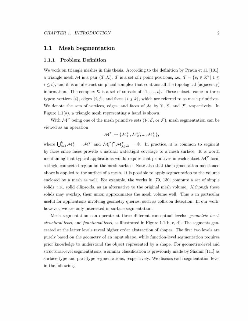
Figure 1.1(a), a triangle mesh representing a hand is shown.
With MP being one of the mesh primitive sets (V, E , or F), mesh segmentation can be
viewed as an operation
MP 7→ MP1 ,MP
2 , ...,MPk ,
where⋃k
i=1MPi = MP and MP
i
⋂MPj,j 6=i = ∅. In practice, it is common to segment
by faces since faces provide a natural watertight coverage to a mesh surface. It is worth
mentioning that typical applications would require that primitives in each subset MPi form
a single connected region on the mesh surface. Note also that the segmentation mentioned
above is applied to the surface of a mesh. It is possible to apply segmentation to the volume
enclosed by a mesh as well. For example, the works in [79, 130] compute a set of simple
solids, i.e., solid ellipsoids, as an alternative to the original mesh volume. Although these
solids may overlap, their union approximates the mesh volume well. This is in particular
useful for applications involving geometry queries, such as collision detection. In our work,
however, we are only interested in surface segmentation.
Mesh segmentation can operate at three different conceptual levels: geometric level,
structural level, and functional level, as illustrated in Figure 1.1(b, c, d). The segments gen-
erated at the latter levels reveal higher order abstraction of shapes. The first two levels are
purely based on the geometry of an input shape, while function-level segmentation requires
prior knowledge to understand the object represented by a shape. For geometric-level and
structural-level segmentations, a similar classification is previously made by Shamir [111] as
surface-type and part-type segmentations, respectively. We discuss each segmentation level
in the following.

CHAPTER 1. INTRODUCTION 3
(a) triangle mesh of a hand model (b) geometric-level
(c) structural-level (d) functional-level
Figure 1.1: A triangle mesh of a hand model (a) and its segmentations at three levels:geometric-level segmentation (b) with each patch being nearly planar and as compact aspossible; structural-level segmentation (c) that decomposes the shape into its constituentparts according to human intuition; and functional-level segmentation (d) that partitionsthe hand into two components — the fingers as a whole and the palm — with respect tothe anatomical property of the hand.

CHAPTER 1. INTRODUCTION 4
1.1.2 Geometric-level Segmentation
Meshes are normally given with only geometry (vertex coordinates) and connectivity (face
adjacency) information. At the geometric level, a shape is partitioned into segments that
possess certain simple surface geometric properties, such as planarity [25] and convexity [23],
or into segments that can be approximated by certain parametric surfaces, e.g. hyperbolic or
parabolic surfaces. The segments do not necessarily correspond to the shape’s constituent
parts as higher order information; they are simply connected homogeneous regions with
similar geometric properties. Geometric-level segmentation extracts the information of a
shape at the lowest level.
Figure 1.1(b) shows a geometric-level segmentation result on the hand model. As we can
see in this particular case, the segments are approximately planar patches that are compact
and the structural information of the hand is not revealed properly.
1.1.3 Structural-level Segmentation
Similar to segmentation at the geometric level, structural-level segmentation is also purely
geometry-based. However, structural-level segments reveal the structure of a given shape.
As the structure of a shape is typically characterized by its constituent parts, segmentation
at this level strives to decompose a shape into its parts. Note that our notion of parts is
generic by referring to the meaningful components of a shape that are intuitive to human
beings. Figure 1.1(c) exemplifies a segmentation on the hand model at structural level.
Compared to geometric-level segments, the five fingers and the palm, which correspond to
the intuitive parts of the hand, are obtained and the structure of the hand shape is revealed.
The concept of a part intuitive to human perception is by no means clearly defined. How
humans perceive parts and how to measure the strength (salience) of parts have long been
studied in psychology and cognition [50, 128]. Despite the absence of a clear definition for
shape parts, the geometry processing community has adopted the minima rule [51] for part
characterization:
All negative minima of the principal curvatures (along their associated lines of
curvature) form boundaries between parts.
The minima rule gives a constructive way to compute parts: mesh segmentation algorithms
may delineate parts by explicitly forming their boundaries from surface regions with nega-
tive minimum principal curvatures [69, 76]. Alternatively, algorithms can also cluster mesh

CHAPTER 1. INTRODUCTION 5
faces into groups by incorporating measures reflecting the minima rule implicitly via con-
siderations of concavity [59]. Since a part is typically convex, it is possible to extract parts
by fitting simple convex geometric primitives, e.g., ellipsoids and cylinders [119, 134], or
by computing convex volumetric regions directly [6, 61]. In addition, techniques are also
designed to find certain specific structures, such as tubular regions [43, 89].
It is worth emphasizing that when we say a part is intuitive to human perception at
the structural level, we emphasize on the intuition based only on the geometry of a shape.
Human intuition about a part could be affected by other higher order information of the
object a shape represents; such parts are at the functional level which is described next. We
are only interested in the structural-level segmentation in this thesis.
1.1.4 Functional-level Segmentation
At the structural level, it is the geometry of a shape that is recognized and the segments
produced are in accordance with the shape’s structure. Functional-level segmentation con-
siders not only a shape itself, but also the object the shape represents. Note that we draw a
clear distinction between an object and its shape. To apply function-level segmentation, an
algorithm needs to understand the functional properties of an object, which in general are
not encoded in the geometry, hence requiring prior knowledge. Segments produced at this
level reflect the functional information of objects based on a specific application context.
Figure 1.1 (d) shows one possible functional segmentation of the hand model. The
hand is divided into two segments, the five fingers as a whole and the palm. Obviously,
the segmentation result in this case follows a functional abstraction of the hand, while
the structural information of the hand shape is not respected. As another example of
functional-level segmentation, one may see the engine body and the pipes attached to it
under the hood of a car as a single intuitive part. We believe this intuition about a part, the
entire engine, has a lot to do with the notion of an engine and how the engine is contrasted
with its surroundings under the hood. For structural-level segmentation, however, we do
not demand our algorithm to understand the pipes are sub-parts of the engine; instead, it
is deemed appropriate to segment the engine into its main body and the pipes, since such a
segmentation is natural based on the engine’s shape only.
Clearly, functional-level mesh segmentation requires algorithms to understand the object
behind an input mesh. This is possible by incorporating prior knowledge using a template
or via training. Similar works for images have been studied, such as in template-based

CHAPTER 1. INTRODUCTION 6
segmentation [16, 46, 85] and image labeling [49, 136]. However, to the best of our knowledge,
such segmentation algorithms for meshes do not exist. This could be in part due to the lack of
a systematic mesh database with segmentation information, which is necessary for training.
1.2 Applications
A common application of mesh segmentation is parameterization, which in turn is useful
to many other applications [114], e.g., detail mapping, mesh editing, and remeshing. Take
texture atlas generation as an example. Since it is in general impossible to parameterize
a mesh surface onto an image plane without stretching, the problem is essentially how to
minimize the stretching of a parameterization. To this end, a mesh surface is partitioned
into approximately developable patches, which can be parameterized individually with less
stretching. Developable surfaces have zero Gaussian curvature everywhere; typical examples
include planes, cones, and cylinders. Segmentation for parameterization applications [56,
72, 107, 108, 121, 145] is at a geometric level in general.
Mesh segmentation is also commonly practiced in reverse engineering, where the goal
is to recover the parametric surfaces from a digitalized shape. This is particularly useful
for CAD models, as CAD software usually only deals with parametric surfaces. Primitive
fitting [54] is a popular strategy for this purpose. Simari and Singh [119], and Wu and
Kobbelt [134] utilize the variational approach [25] to approximate surfaces with planes,
spheres, cylinders, rolling-ball blend patches, and ellipsoids. This approach is extended
by Yan et al. [139] to incorporate general quadric surfaces. To speed up the processing,
hierarchical primitive fitting is adopted by Attene et al. [4]. Except for primitive fitting,
other techniques such as slippage [41] and curvature tensor analysis [68] are also utilized,
based on the observation that surface patches with similar slippage or curvature tend to
form a single parametric surface. Depending on the types of the fitting primitives, such
segmentations may sit at a geometric or a structural level. For example, if ellipsoids are
used, the resulting segments are likely to correspond to intuitive parts.
Animation makes use of mesh segmentation as an important auxiliary operation as
well. In order to generate a high quality deformation sequence of an articulated shape, it
is beneficial to represent the shape via its skeleton, because the skeleton can be animated
easily and the surface is then reconstructed from the deformed skeleton. Due to the strong

CHAPTER 1. INTRODUCTION 7
connection between the parts of a shape and its skeleton, quite a few skeletonization al-
gorithms [59, 76, 110] are segmentation-based. Once the parts of an articulated shape are
segmented out, skeletons can be readily constructed from these parts. Another example
where mesh segmentation comes handy is morphing [116, 148]. To enhance the quality of
morphing, both the source mesh and the target mesh are segmented into compatible parts,
and morphing is carried out between the matched pairs. Collision detection, a necessary
operation in a number of applications including gaming and physical simulation, could also
benefit from mesh segmentation. As shown in [40, 74], meaningful segments would help
build a well structured hierarchical bounding volume tree that is crucial to the efficiency of
collision detection. As the above applications usually need to have the resulting segments
reflect the structure of a shape, these segmentations are at a structural level.
Mesh coding is another area where segmentation is useful, from several aspects. From
the computational complexity perspective, partitioning a surface into segments helps reduce
the overhead in a divide-and-conquer manner. In the work by Karni and Gotsman [58], a
surface is decomposed into multiple patches and encoded separately, avoiding the eigenvalue
decomposition of an otherwise large matrix. Coding mesh patches separately is also error-
resilient and space-efficient; Yan et al. [140] show that carefully designed segmentation
algorithms are capable of producing patches suitable for efficient coding and robust against
patch corruption. To further optimize the transmission over a bandwidth-limited channel,
e.g., wireless network, mesh patches are deliberately constructed in the coding stage. During
transmission, only the patches visible to end users are transmitted or transmitted with higher
priority. The experiments in [45, 141] attest to the effectiveness of this strategy. Different
from the above works, time-dependent geometry coding is studied by Lengyel [71], in which
mesh vertices are clustered into groups with similar trajectories along the time axis so that
they can be encoded in a local coordinate system. Segmentations are all at a geometric-
level for these applications except for the last one, in which the mesh vertices with similar
trajectories often form a rigid structural part of a shape.
Last but not least, mesh segmentation also plays an important role in shape modeling and
shape recognition. One example shape modeling task is to model objects by parts. The ob-
servation herein is that objects can be classified into categories with similar part structures;
therefore similar parts can be reused to allow for efficient reconstruction of new models with
high details. In order to obtain reusable parts from shapes, both semi-automatic [39, 55] and
automatic [61] segmentation techniques are proposed. Shape recognition is a hard problem

CHAPTER 1. INTRODUCTION 8
in general. As lower geometric information, e.g., curvatures, is not sufficient to manifest
higher order semantic information about a shape, higher level information needs to be ex-
tracted to recognize the shape better. To this end, algorithms often make use of the parts of a
shape and their topological relations. Such an example is from shape retrieval [31, 110, 148],
in which the signature of a shape is calculated based on the features and the relations be-
tween its structural parts. In fact, researches in psychology and cognition [15, 50, 51] have
long shown that shape parts have a profound impact on the way human beings recognize
and understand shapes. Although related studies on this topic are primarily cast on image
data [2, 57, 62, 67, 105, 117], 3D shape representation with structural information and its
application has received much attention [1]. We believe mesh segmentation is indeed an
indispensable ingredient in this promising area and deserves long-term study.
1.3 Contributions
The difficulty of structural-level segmentation lies in the fact that the notion of parts in a
shape is not well-defined. In this thesis, we propose several ideas to address this problem.
Some of these ideas, including the part-aware metric, segmentability, and salience-driven
cut search, not only lead to quantitative measures for characterizing parts, but also suggest
constructive means to compute them. Our algorithms have been demonstrated to produce
high quality segmentation results. We elaborate our contributions as follows.
A novel metric to capture part information In order to apply spectral clustering to
mesh segmentation, we need a distance metric that is able to capture the part information
of a shape. Designing a part-aware metric on mesh surfaces is non-trivial since the parts are
yet to be found. In practice, one is supposed to utilize the metric to facilitate segmentation.
Therefore, the realization of an effective metric should be conceptually simple, at least not
more complicated than implementing a third party segmentation algorithm and using the
resulting parts to help build the metric. We design such a metric based on the characteristics
of how visible regions change for points within shapes and across part boundaries. To date,
our metric is the only one that is specifically designed to capture part information. It
is demonstrated to outperform existing metrics [30, 59, 66] that have been utilized for
mesh segmentation. Note that our part-aware metric is also useful for a variety of other
applications in geometry processing.

CHAPTER 1. INTRODUCTION 9
Application of spectral clustering to mesh segmentation We for the first time ap-
ply spectral clustering to mesh segmentation, effectively and efficiently. Spectral clustering
is a popular clustering algorithm studied in machine learning. Resorting to the part-aware
metric, we design yet another variant of spectral clustering for structural-level segmentation.
To make our algorithm effective in practice, we address several problems of spectral cluster-
ing within the context of mesh segmentation. For efficiency, we make use of sub-sampling
and the Nystrom method [10] to reduce the complexity involved in pairwise distance compu-
tation and eigenvalue decomposition. We provide a geometric interpretation to the Nystrom
method and reach a measure for its approximation quality. From this, practical sampling
schemes are suggested. Since our algorithm transforms the part-aware distances into an Eu-
clidean embedding and finds an approximate solution to a global optimization problem, it is
able to produce high quality segmentation results. This segmentation algorithm is efficient,
operating in a k-way partition manner, where k is the number of segments input by users.
Segmentability- and salience-driven segmentation via spectral embedding We
further improve our segmentation algorithm by enhancing its autonomy and quality. The
improved algorithm segments through recursive 2-way cuts. The current mesh piece is only
segmented when it has a sufficiently large segmentability score. The segmentability measure
is derived by spectral-embedding a mesh piece into 2D, in which its part information is
better revealed and readily quantified. Unlike the previous algorithm where users need to
specify k for each input model, the improved algorithm enjoys a higher autonomy with a
fixed segmentability threshold that is model-independent. Meanwhile, we apply salience
to enhance segmentation quality. Salience is an important concept studied in psychology
to measure the strength of a part and it is closely related to how humans perceive parts.
Although salience has been previously used for mesh segmentation, it is only used in post-
processing, probably due to the difficulty of incorporating it into the initial search for parts.
We found a solution to this by carefully arranging mesh faces into a sequence which can be
considered as derived through a 1D spectral embedding. Since the cut is only sought along
the sequence, the search space for parts is substantially reduced. As a result, we can afford to
integrate salience into the search procedure. As the face sequence preserves the meaningful
cuts and salience is exploited early on, this algorithm achieves superior segmentation quality.

CHAPTER 1. INTRODUCTION 10
1.4 Thesis Organization
The reminder of the thesis is organized into six chapters. In Chapter 2, we review mesh
segmentation techniques and spectral clustering. The part-aware metric is developed in
Chapter 3. Using this metric, we design a k-way mesh segmentation algorithm using spectral
clustering in Chapter 4. Chapter 5 studies and applies sub-sampling to this segmentation
algorithm to reduce its complexity. Next, Chapter 6 improves upon the k-way segmentation
algorithm via recursive 2-way cuts based on segmentability and salience. We conclude our
work and point out future directions in Chapter 7.

Chapter 2
Background and Related Work
This chapter presents a review of the related literature. In order to understand mesh
segmentation better, we first highlight certain differences between mesh segmentation and
image segmentation in Section 2.1. After this, we review some existing mesh segmentation
techniques in Section 2.2. Section 2.3 discusses spectral clustering briefly.
2.1 Mesh Segmentation vs. Image Segmentation
Segmentation has been studied extensively on image data. Image segmentation is of fun-
damental importance in many fields including computer vision, medical imaging, and video
coding [3]. A tremendous amount of work has been conducted in the last several decades.
A recent search in EI Compendex showed a total of 9154 records of papers with “image
segmentation” in title from the year of 1970 to 2008. Before we discuss the differences be-
tween mesh segmentation and image segmentation, we briefly discuss image segmentation
first. Interested readers are referred to the surveys in [47, 95, 99] for more details.
It is commonly practiced in computer vision to segment images along the boundaries
of the objects in a scene. Boundaries between objects are often detected in regions with
dramatic intensity changes, say by the Canny edge detector [20]. However, color images
with abundant textures and patterns easily produce many spurious edges, which do not cor-
respond to real object boundaries. To tackle this problem, statistical methods are applied to
select only salient edges and connect them into continuous boundaries [103, 133]. Another
approach to detecting meaningful boundaries is through supervised learning. Such an ex-
ample is in [84], where the authors make use of ground truth images with manually-marked
11

CHAPTER 2. BACKGROUND AND RELATED WORK 12
boundaries to train a classifier. Posterior probabilities of test image pixels on boundaries
are calculated via the trained classifier. In addition, it is also possible to segment images
via pixel grouping, where image pixels are clustered into regions directly without forming
explicit boundaries. Both the spectral technique [115] and the statistical technique [127] fall
into this category.
Image segmentation is also an indispensable step in medical image analysis. Before
anatomical structures captured in images by, e.g., computer tomography (CT) and mag-
netic resonance imaging (MRI), can be analyzed, they must be segmented out from their
surroundings. This is known as the delineation of anatomical structures. One popular
technique for this is deformable models. Boundary-based deformable models [63, 86] use a
parametric contour, which evolves on images to reduce its energy until a local minimum is
reached. As an energy functional encodes the desired properties of both the contour and
the target positions, the delineated boundary is often of higher quality. To better incorpo-
rate prior knowledge, template-based deformable models [16, 46, 85] are developed as an
alternative. Template deformable models are programmed to assume the generic shape of
the target structure, which amounts to encoding prior knowledge. Meanwhile, they are also
allowed to deform moderately to accommodate the slight differences from multiple instances
of the structure.
Mesh segmentation has certainly benefited from the research achievements of image seg-
mentation. In fact, as one of the early mesh segmentation techniques, the watershed algo-
rithm by Mangan and Whitaker [82] is extended from its counterpart in image segmentation.
Meanwhile, mesh segmentation is also a quite different topic from image segmentation; their
differences can be understood from several perspectives as follows.
In terms of the types of information contained in the data, images have intensity and
spatial information. These two types of information are different stimuli to human percep-
tion and they play different roles in deriving segmentation results. Roughly speaking, an
image segment is typically a spatially continuous region with similar intensities or patterns
(textures) [8, 96]. For mesh segmentation, however, current research is only concerned with
the shape of a mesh, i.e., a spatial information. Any other information, if any, such as color
and texture, is discarded.
One may view a 2D image as a mesh by virtually lifting its pixels vertically, where
the elevation of each pixel is determined by its intensity. However, unlike the pixels of an
image, the vertices of a mesh have irregular connectivity in general. For this reason, meshes

CHAPTER 2. BACKGROUND AND RELATED WORK 13
lack a global canonical parameterization. This may prevent certain useful techniques from
being used for meshes, such as the Fourier Transform. Essentially, meshes are 2D manifolds
embedded in 3D and their dimensionality is atypical.
Mesh segmentation is a relatively new research topic in contrast to image segmentation.
Due to their differences, techniques for image segmentation cannot be trivially extended to
mesh segmentation. So far, mesh segmentation has not seen the use of certain advanced
techniques, including supervised clustering. This is in part due to the absence of a systematic
mesh database with segmentation information for training purposes.
2.2 Segmentation Techniques
Mesh segmentation algorithms can be categorized via many criteria. In this section, we re-
view some existing algorithms based on their characteristics and how much user intervention
they require.
2.2.1 Bottom-up and Top-down
If a mesh segmentation algorithm seeks segments using global information, e.g., by comput-
ing a (approximate) solution to a global optimization problem, we call it top-down. On the
other hand, if an algorithm finds segments using only local information, e.g., via a greedy
approach, we call it bottom-up. In the bottom-up category, final segments are typically
formed by grouping smaller ones, for example, starting from individual faces. The segmen-
tation procedure is often guided by a cost function, which is minimized locally in a greedy
manner. Bottom-up approaches are usually efficient. However, they are subject to local
minima and over-segmentation. Top-down approaches address these problems by working
in the opposite direction: segments are obtained by decomposing a mesh into pieces, through
either a simultaneous k-way cut, or a sequence of cuts (typically 2-way cut) in a hierarchical
manner. Since top-down approaches optimize segmentation using more global information
than bottom-up approaches, they tend to achieve better results, but usually with a higher
computational cost.
Bottom-up and top-down only roughly characterize the properties of existing mesh seg-
mentation techniques. In the following, we further split them into seven sub-categories and
discuss their characteristics, pros, and cons briefly. Note that the categorization is neither
perfectly disjoint nor complete; we only investigate some popular techniques and try to

CHAPTER 2. BACKGROUND AND RELATED WORK 14
classify them according to their most prominent characteristics. Readers are referred to
[5, 111] for more detailed coverage.
Region growing is a bottom-up approach, in which a segment is formed by growing a
continuous surface region until the regulatory constraints fail. In sequential region grow-
ing [68, 82, 102, 146, 147, 148], the next region starts to grow after the previous one cannot
grow any more. This process iterates until the entire surface is covered. In simultaneous
region growing [55, 72, 94, 137, 144], multiple regions are seeded and grown simultaneously:
the immediate region to grow is always the one with the smallest growing cost. The asymp-
totic complexity for sequential growing is typically O(n) (n is the face count) since each mesh
face is visited only once, while simultaneous growing usually sees a complexity of O(n log n)
due to the maintenance of a global priority queue. At a higher complexity, simultaneous
growing often offers better segmentation quality because of its fine-tuned growing order
with smaller granularity. Region growing methods are fast and the framework is generic.
By applying different growing constraints, region growing methods are capable of achieving
both geometric-level and structural-level segmentations. As bottom-up approaches, how-
ever, region growing methods are susceptible to local minima.
Region merging methods [4, 40, 41, 113] start out by partitioning an entire mesh surface
into patches, each typically containing a single face initially, and recursively merge neigh-
boring patches. Similar to simultaneous region growing, the merging order is also guided by
a priority queue. As an example, Garland et al. [40] combine three error metrics to prioritize
all current possible merges, ensuring that each resulting segment is compact, nearly planar,
and has consistent face normals. It is worth mentioning one recent work [6] based on region
merging for computing convex parts, which works on volumes rather than on surfaces. The
algorithm decomposes the volume enclosed by a mesh into tetrahedra; neighboring solids
(initially consisting of a single tetrahedron) are then merged recursively. Unlike surface-
based convexity measures, the convexity measure for solids enjoys higher accuracy. The
most significant advantage of the region merging framework is its ability to create a seg-
mentation hierarchy and this is important to applications involving spatial queries. Region
merging is also bottom-up, and its small merging cardinality, usually 2 (merging only two
adjacent patches each time), may deteriorate the segmentation quality.

CHAPTER 2. BACKGROUND AND RELATED WORK 15
Variational approaches [25, 56, 59, 61, 65, 98, 116, 119, 134, 139] are probably the most
popular technique for mesh segmentation, which essentially solve the K-means clustering
problem [80] using Lloyd’s algorithm [78]. In short, Lloyd’s algorithm finds an approximation
(a local minimum) to the global optimal solution by alternating two operations, element
assignment and proxy fitting, until convergence. In the element assignment operation each
mesh face is assigned to the cluster whose proxy is closest to this face; in the proxy fitting
operation each proxy is refined to better fit, according to a chosen metric, the member faces
of its associated cluster. For example, if the goal is to partition a surface into planar patches,
a proxy should be the best fitting plane of its cluster. In practice, proxies often converge
with high rate. A variational method is top-down as all clustering elements are examined
simultaneously to optimize for a cost function. However, k, the number of desired segments
is non-trivial to infer from input data and is usually given by users.
Boundary formation [69, 75, 92] methods seek to delineate segments explicitly with
their boundaries. In contrast, techniques mentioned above all construct segments by group-
ing mesh primitives. A segment boundary is a closed contour typically formed by a sequence
of mesh edges. Such contours are either formed by connecting broken feature lines from con-
cave regions as in [69, 92] or computed as a graph cycle with minimum weight as in [75].
Boundary formation methods are top-down. As segment boundaries are formed explic-
itly, it is easier to make them clean and smooth. Due to the obliviousness to the interior
of the resulting segments, however, boundary formation approaches have only been used
for structural-level segmentation. In addition, this method is subject to featureless regions
where intuitive part boundaries are supposed to cross. Completing broken contours through
such regions is challenging.
Statistical approaches [30, 42, 64] are gaining increasing attention recently. Lai et
al. [64] model the distance between faces using random walks. Each edge of a triangle
face is associated with a probability describing how likely a random walk moves across
this edge to the neighboring face. The algorithm allows users select to (or automatically
select) several seed faces to represent the desirable parts of an input mesh. Each face
is clustered into the part of a seed face if a random walk starting from the face has the
highest probability of reaching this seed face. The whole modeling process is reduced to
solving a sparse linear system. For structural-level segmentation, the probabilities assigned
to edges are related to local concavities. The algorithm proposed by de Goes et al. [30] is

CHAPTER 2. BACKGROUND AND RELATED WORK 16
in the same vein, by modeling diffusion distance on surfaces. Golovinskiy and Funkhouser
propose a randomized approach [42]. Roughly speaking, the idea is to apply several popular
segmentation algorithms with different or random initial settings for a large number of
times. Each particular execution produces a set of boundary edges. With the results from
all executions, the algorithm computes a probability of each edge being on a part boundary.
A concrete segmentation is computed based on such probabilities. Statistical approaches,
especially the first two algorithms based on random walks and diffusion distance, are in
general top-down techniques. Also they have been empirically shown to be robust against
noise. Statistical approaches are so far only applied to structural-level segmentation.
Topology-driven approaches [7, 74, 104, 126, 135] are top-down segmentation tech-
niques, which utilize shape skeletons. Note that the skeleton herein refers to a 1D curve that
roughly lies inside a shape and reflects its structure. Shape skeletons are suggestive of shape
parts. Think of an articulated shape, such as a human being, whose skeleton can be divided
into sections at the critical points, e.g., branch points, with resulting sections correspond-
ing to the intuitive parts, i.e., torso, limbs, and head. That being said, topology-driven
approaches are in general divided into three steps: extract skeleton, identify critical points,
and associate skeleton sections with shape parts. Since the topology of the skeleton is pose-
invariant to the articulation of a shape, topology-driven approaches are invariant to poses.
However, robust skeleton extraction and critical points identification are both non-trivial.
Meanwhile, only structural-level segmentation is possible through this technique.
Symmetry-driven approaches are based on the observation that both natural and man-
made objects are usually symmetric to a certain degree [73], either globally or partially. It is
then rational to exploit symmetry information for segmentation. Simari et al. [118] propose
to partition a mesh iteratively using weighted principal component analysis to find extrinsic
reflectional symmetries. In each iteration, a subregion of the current mesh piece is extracted
and partitioned into two by a plane if the subregion is symmetric with respect to the plane.
Podolak et al. [100] introduce Planar-Reflective Symmetry Transform to compute major
local symmetric planes of a shape and such planes are used to simultaneously segment
the shape into self-symmetric parts. Different from the above two algorithms, Mitra et
al. [87] detect surface regions that are invariant up to rigid transformations and scaling.
This is achieved through a voting scheme in a transformation space. Symmetry-driven
segmentation is useful to many applications, including mesh coding, shape retrieval, and

CHAPTER 2. BACKGROUND AND RELATED WORK 17
Technique Strategies Level Pros / ConsRegion Growing B G, S efficient, generic / prone to local op-
timumRegion Merging B G, S hierarchical result / prone to local
optimumVariational Approach T G, S better approximation to global opti-
mum / unknown number of clustersBoundary Formation T S clean and smooth boundary / chal-
lenging to complete broken bound-aries over featureless regions
Statistical Approach T S mathematically sound, resistant tonoise / unknown number of clusters
Topology-driven Approach T S pose-invariance / non-trivial skele-ton extraction and critical pointsidentification
Symmetry-driven Approach T S informative segments / only extrin-sic symmetry so far, not necessarilystructural parts
Figure 2.1: Highlights of various segmentation algorithms. B: bottom-up, T: top-down, G:geometric-level, S: structural-level.
remeshing. The segments obtained by symmetry-driven approaches are typically informative
about the structure of a shape. However, depending on a shape’s symmetry structure,
such segments may not necessarily correspond to the intuitive parts of the shape as in
the structural-level segmentation. In addition, current symmetry-driven approaches handle
only extrinsic symmetries, but not intrinsic ones. For example, a bent left arm would not
be considered symmetric with respect to a straight right arm.
Figure 2.1 highlights the properties of the segmentation algorithms mentioned above.
2.2.2 User Intervention
We can also classify mesh segmentation algorithms based on the degree of user intervention.
In this thesis, we adopt three classes: automatic, semi-automatic, and manual.
In our classification, an automatic segmentation algorithm simply needs users to feed
a mesh and the segments are produced automatically. Note that we do allow automatic
algorithms to have free parameters, such as threshold values. Users can fine-tune these
parameters in order to suit different input models. We consider parameter setting as a

CHAPTER 2. BACKGROUND AND RELATED WORK 18
robustness issue, rather than an autonomy issue. We mention one special parameter, the
number of segments. The number of segments is directly related to segmentation output
and it is highly model-dependent. The variational approaches mentioned above are good ex-
amples where the number of segments is needed. Of course, it is ideal to have an automatic
algorithm perform robustly on all kinds of meshes with a fixed set of parameters. Unfortu-
nately, this is difficult, especially for the structural-level segmentation. The majority of the
available mesh segmentation algorithms, e.g., [40, 61, 76, 82, 93], are automatic.
For semi-automatic algorithms [55, 144], users are usually required to provide direct
assistance for segmentation, such as drawing sketches on a mesh to indicate desired segments.
Take the work by Ji et al. [55] for example. Users must first provide one stroke on the
background part and the other on the foreground part of a given mesh. Then a region
growing approach is executed to identify the two corresponding parts, as in an automatic
algorithm. In order to achieve better segmentation results, users may want to make the two
strokes longer and place them in parallel to the desired boundary. The algorithm developed
by Lee et al. [69] also allows for direct user assistance. Semi-automatic algorithms strike the
balance between autonomy and user assistance. They are in general capable of obtaining
higher segmentation quality than automatic algorithms.
If an algorithm requires a significant amount of segmentation information from users, we
consider it manual. For example, users may be asked to sketch the boundaries between all
desirable segments, while the algorithm only helps connect nearby broken boundary sketches
and smooth them. Conceptually, manual segmentation is more a tool than an algorithm. To
the best of our knowledge, there is not a systematic manual segmentation tool yet. However,
such a tool could be useful, especially when it comes to building a segmentation benchmark
for structural-level mesh segmentation. Generating ground-truth segmented models could
involve a large amount of strenuous and tedious work; having a handy segmentation tool
should greatly improve the efficiency.
2.3 Spectral Clustering
In this section, we briefly review spectral clustering that has inspired our work. Spectral
clustering refers to any partitioning algorithm that utilizes eigenvectors (and eigenvalues) of
an appropriately defined matrix which captures the domain knowledge. Spectral clustering
has its root in spectral graph theory [24, 35] and has seen a tremendous amount of work [9,

CHAPTER 2. BACKGROUND AND RELATED WORK 19
18, 37, 90, 97, 143] over the past decade. Spectral clustering can work either in 2-way, i.e.,
clustering data into two groups (recursively), or in k-way, i.e., clustering data into k groups
simultaneously. Interested readers are referred to a recent survey [36] for details.
2.3.1 Classical Examples
Given a set of data points Z = zi, |Z| = n, and an affinity matrix W ∈ Rn×n, where Wij
encodes the relation between zi and zj , clustering the data points in Z can be viewed as a
graph partitioning problem, in which Z is the set of graph nodes and Wij defines the weight
of edge (i, j). Note that in different algorithms, W may be modeled to describe either the
similarities or the dissimilarities between data: if similarity (dissimilarity) is modeled, a
larger Wij implies a more similar (dissimilar) pair of points.
Assuming that W encodes similarity information, the goal in the first example is to
partition the graph nodes into two well-separated sets Z1 and Z2 such that
Cut(Z1,Z2) =∑
zi∈Z1, zj∈Z2
Wij
is minimized. Denote by v the membership indicator vector (v(i) = −1, if zi ∈ Z1, and
v(i) = 1, if zi ∈ Z2; note that v(i) represents the i-th entry of v), we have
Cut(Z1,Z2) =14
∑
i,j
Wij(v(i) − v(j))2 =12vT (D −W )v,
where D = diag(D00, . . . , Dnn) is a diagonal matrix whose diagonals are row sums of W , i.e.,
Dii =∑
zj∈Z Wij . By relaxing the entries in v from discrete values to continuous values,
subject to the constraint ‖v‖2 = 1, it can be shown that the minimum value of Cut(Z1,Z2)
is achieved when v is the eigenvector of D−W that corresponds to the smallest eigenvalue.
However, since D −W has the smallest eigenvalue 0 and its corresponding eigenvector is a
constant vector, v is taken as the second smallest eigenvector to avoid the trivial solution.
Due to the relaxation, the eventual clustering is Z1 = zi|v(i) < 0, Z2 = zi|v(i) ≥ 0.This result is shown in [35]. For simplicity, we will from now on refer to an eigenvector as
large or small based on its corresponding eigenvalue, i.e., the largest eigenvector refers to
the eigenvector with the largest eigenvalue.
As the Cut measure undesirably favors small sets of isolated nodes, Normalized Cut is
proposed in [115] to deal with this problem. For Normalized Cut, the quality measure is
NCut(Z1,Z2) = Cut(Z1,Z2)( 1
V ol(Z1)+
1V ol(Z2)
),

CHAPTER 2. BACKGROUND AND RELATED WORK 20
1. Build an affinity matrix W , set its diagonals to 0, and process W ← D− 12 WD− 1
2 .
2. Compute the eigenvalue decomposition W = V ΛV T , where V = diag(λ1, λ2, . . . , λn)and λ1 ≥ λ2 ≥ . . . ≥ λn, select the largest k eigenvectors from V and stack them intothe columns of matrix U , i.e. U = [V1|V2| . . . |Vk].
3. Normalize each row of U , i.e., Uij ← Uij/‖Ui.‖.4. Considering the rows of U as the Euclidean-embeddings of Z, i.e., the i-th row is the
embedding of zi, cluster Z into k clusters.
Figure 2.2: NJW spectral clustering algorithm.
where V ol(Zi) =∑
zj∈ZiDjj . Djj measures the “degree” of zj and V ol(Zi) is the “volume”
of Zi. Since NCut is normalized by the volume of each cluster, the clustering result no
longer favors small clusters as Cut does. Unfortunately, computing the optimal solution
that minimizes NCut is NP-complete; therefore, the authors suggest to find an approximate
solution by computing the second smallest eigenvector of the generalized eigenvalue problem
(D −W )v = λDv,
and thresholding this eigenvector to derive the final cut.
Both spectral clustering algorithms mentioned above have clearly defined quality func-
tions to optimize for. On the other hand, some spectral clustering algorithms are only
empirically demonstrated or loosely proved to be able to discern the meaningful clustering
structures present in a given data set. Such an example is the NJW algorithm by Ng,
Jordan and Weiss [90], which runs as in Figure 2.2. The rationale behind this algorithm is
revealed by considering the ideal case, in which the inter-cluster points have zero similarities
(infinite distances). Without loss of generality, we assume that the points from the same
cluster are numbered continuously; hence the affinity matrix W is block-diagonal. If there
are k such ideal clusters, it is able to show that the embedded points (rows of U) from the
same cluster would be mapped to a single point on the unit sphere. Essentially, there are
k distinct points from k mutually orthogonal directions, which is easy to cluster. In reality
when the inter-cluster affinities are non-zero, it can be viewed that a perturbation is added
to W . It is shown that if W is still almost block diagonal and the size of each cluster and
the degree of each node do not vary much, similar properties are still expected.

CHAPTER 2. BACKGROUND AND RELATED WORK 21
1. Build an affinity matrix W , which models the relations (similarities or dissimilarities)between each pair of data points in Z. W is subject to further processing.
2. Compute the eigenvalue decomposition W = V ΛV T , and use the eigenvalues and theeigenvectors to obtain an Euclidean embedding of Z.
3. Cluster the embedded data points.
Figure 2.3: Standard paradigm of spectral clustering.
2.3.2 Generic Paradigm
A typical spectral clustering algorithm is comprised of three steps as shown in Figure 2.3.
The first step builds an affinity matrix W that models the relationships among the data
points in Z. The information encoded in W reflects the domain knowledge about the prob-
lem at hand. In the second step, the eigenvectors (and eigenvalues) of W are used to derive
an Euclidean embedding of Z; this embedding is typically called spectral embedding. Spec-
tral embedding per se has been studied intensively, in the context of manifold learning and
dimension reduction. Famous examples include Local Linear Embedding [106], Isomap [125],
and Laplacian Eigenmap [11]. They all share the common feature of utilizing local infor-
mation to capture curved manifolds embedded in higher dimensional ambient space. In
the last step, the actual clustering operation is applied to the embeddings. There are a
variety of ways to implement the clustering, including the popular K-means algorithm [78].
The affinities in W determine the spectral embedding, and hence influence the quality of
the clustering result. Therefore, it is crucial to compute meaningful affinities using the
domain knowledge about the problem at hand. Spectral embedding transforms the affinity
information in W into an Euclidean embedding, usually with low dimensionality, and the
subsequent clustering operation is readily implemented.
Spectral clustering techniques are diverse and a universal spectral clustering algorithm
that performs well on all kinds of data does not exist. There are several difficult questions
related to spectral clustering, such as how to choose the right kernel width for building
the affinity matrix W and how to cluster in the spectral embedding space [37, 83]. In the
subsequent chapters, we design spectral clustering algorithms suitable for the purpose of
mesh segmentation; various related problems are solved within our application context.

Chapter 3
Part-aware Metric
3.1 Overview
Since we apply spectral clustering to mesh segmentation and a crucial prerequisite for ap-
plying spectral clustering is to encode the domain knowledge of the problem at hand in an
affinity matrix, in our application, we need a metric to prescribe distances between the faces
of a given mesh. In this chapter, we only develop such a metric. How to use the metric to
define an affinity matrix for spectral clustering is left to the next chapter.
The distances between mesh faces prescribed by our metric should be suitable for
structural-level segmentation. In other words, we want distances between the faces from the
same part to be small, while distances between the faces from different parts to be large.
However, defining such a distance measure is challenging, since the concept of a “part” is
not well-defined. Moreover, the distance measure should be simple to compute yet effective
for the subsequent segmentation task; we shall not run a third party segmentation algorithm
to find the parts of a mesh first and then compute distances between the faces accordingly.
In this chapter, we derive three distance measures: geodesic, angular, and VSI distances,
in Section 3.2, Section 3.3, and Section 3.4, respectively. The VSI distance is most effective
in encoding part information, and the other two complement the VSI distance in different
scenarios. The resulting part-aware metric, described in Section 3.5, is a combination of
the three. Since our part-aware metric is of generic interest, we show its use in several
non-segmentation geometry processing applications in Section 3.6. A summary is given in
Section 3.7. In subsequent chapters, we show how the metric is used for mesh segmentation.
22

CHAPTER 3. PART-AWARE METRIC 23
3.2 Geodesic Distance
Consider two faces on a mesh surface. In general, they tend to belong to different parts if they
are geodesically far apart and vice versa. This is in accordance with the Gestalt principle
of proximity [88] about perception. Therefore, the first distance measure we employ is the
geodesic distance between faces.
Computing accurate geodesic distances [122] on surfaces is quite involved and not neces-
sary for our purpose. Instead, we make use of the dual graph of a mesh to derive approximate
geodesic distances between faces. A mesh dual graph, G, is constructed by representing the
faces of a mesh by nodes and connecting the nodes whose corresponding faces share a com-
mon edge. This is illustrated in Figure 3.1(a).
(a) (b)
Figure 3.1: Mesh dual graph and approximate geodesic weight between adjacent faces. In(a), the dashed blue lines are the edges of the dual graph G; G(i, j) denotes the edge incidentto faces fi and fj . (b) shows how the weight of G(i, j) is computed.
G stores the connectivity information of the faces. Note that for a triangle mesh without
boundary, G is a graph whose nodes all have degree 3. Given an edge G(i, j), we denote by
pc the middle point of the common edge shared by fi and fj , and by pi and pj the centroids
of fi and fj , respectively. The weight of G(i, j) is defined as
weight(G(i, j)
)= ||pi − pc||+ ||pj − pc||. (3.1)
This is shown in Figure 3.1(b).
With the edge weights defined, the geodesic distance between any two faces is approx-
imated by the shortest graph distance between their corresponding nodes in G. From now

CHAPTER 3. PART-AWARE METRIC 24
on, we refer to the dual graph with geodesic edge weights as Gg.
Note that in general, geodesic distance alone does not reflect part structure robustly,
which can be seen from Figure 3.2(a). Nonetheless, geodesic distance is important in some
part-related applications (see Section 3.6). Even for mesh segmentation, it can be exploited
to improve segmentation quality. We shall see such examples in Chapter 4 and Chapter 6.
3.3 Angular Distance
Angular distance is similarly obtained through another mesh dual graph Ga. Ga has the
same structure with Gg, but with different edge weights. Given two adjacent faces fi and
fj with normals ni and nj , respectively, the weight of edge Ga(i, j) is defined as
weight(Ga(i, j)
)=
acos(ni · nj)/π if fi and fj form a concave dihedral angle,
ε if fi and fj form a convex dihedral angle.(3.2)
We set ε = 0.001 to emphasize concave angles: the more concave a region is, the larger the
weights are. This is roughly in accordance with the minima rule (Section 1.1.3). With Ga,
the angular distance between any two faces is their shortest graph distance in Ga.
Figure 3.2 shows a geodesic distance field and an angular distance field on a dolphin
model. As we can see from this example, the geodesic distance fails to induce large distances
across the concave boundary regions between the body and the fins/beaks, while the angular
distance manifests large distance jumps across those regions. Note that in this thesis, we
color plot scalar fields by linearly interpolating the hue values in the HSL color space; bluish
colors indicate small field values and reddish colors indicate large field values. Since we are
not interested in the exact values of a distance field but its relative variations across a mesh
surface, we do not show color bars in such figures.
Although it reflects the parts of a shape when concave regions are present, angular
distance suffers from what we call the leakage problem. This is caused by defining edge
weights using only local surface properties. Figure 3.3 contrasts a geodesic distance field
with an angular distance field on a synthetic “snake” model to illustrate this problem. From
Figure 3.3(b), we see that although a concave region separates the left vertical part from the
horizontal part, the concave region itself does not form a closed loop between the two parts.
Therefore the shortest path between the two parts goes through the flat region to avoid the
concave region, as indicated by the magenta curve. As a result, the angular distance field

CHAPTER 3. PART-AWARE METRIC 25
(a) geodesic distance field (b) angular distance field
Figure 3.2: Example geodesic and angular distance fields on a dolphin model, where thered sphere indicates the source face. From the angular distance field, we see large distancejumps across the concave regions between the parts; this phenomenon is not observed fromthe geodesic distance field.
(a) geodesic distance field (b) angular distance field
Figure 3.3: Example geodesic and angular distance fields on a snake model. We see thatthe angular distance field is not sufficiently different from the geodesic distance field due tothe leakage problem. The red sphere indicates the source face.

CHAPTER 3. PART-AWARE METRIC 26
(a) (b) (c) (d)
Figure 3.4: Visible regions of a point (red dot) as it travels inside a shape. Comparing (a)and (b), or (c) and (d), we see the shape of visible regions are similar when the point staysin the same part. There is a large change in the shape of the visible region as the pointcrosses the part boundary, as shown in (b) and (c).
looks almost the same with the angular distance field, failing to reflect the part structure of
the snake model.
3.4 VSI Distance
In retrospect, although separation between parts inevitably involves concavity, to capture
it one is not restricted to surface measurement. The inherent limitation of surface mea-
surement can be addressed from a more global and volumetric view for part analysis. This
leads to the realization that shape concavity can be manifested inside the shape’s volume
via occlusion or visibility considerations.
Specifically, we examine a 3D object from within its enclosed volume and measure the
visibility of the object surface from appropriately chosen reference points in the volume.
Unlike a “part”, a visible region is clearly defined. Since parts are generally convex, the
visible regions from within a part remain stable or change only gradually while moving
inside the part. In contrast, when moving across a part boundary to another part, the
visible region undergoes large change due to the concave regions separating the two parts.
Such a property is exemplified in Figure 3.4. In this section, we exploit this idea and develop
a robust part-aware distance measure based on the difference of visible regions.

CHAPTER 3. PART-AWARE METRIC 27
Figure 3.5: Three steps to compute VSI distance. In step 1, two example faces (supposethey are adjacent), fi and fj are mapped to their reference points ri and rj . In step 2, thevisible regions at ri and rj are sampled and stored in their VSIs, Si and Sj . In step 3, Si
and Sj are used to derive the distance between fi and fj in graph Gv.
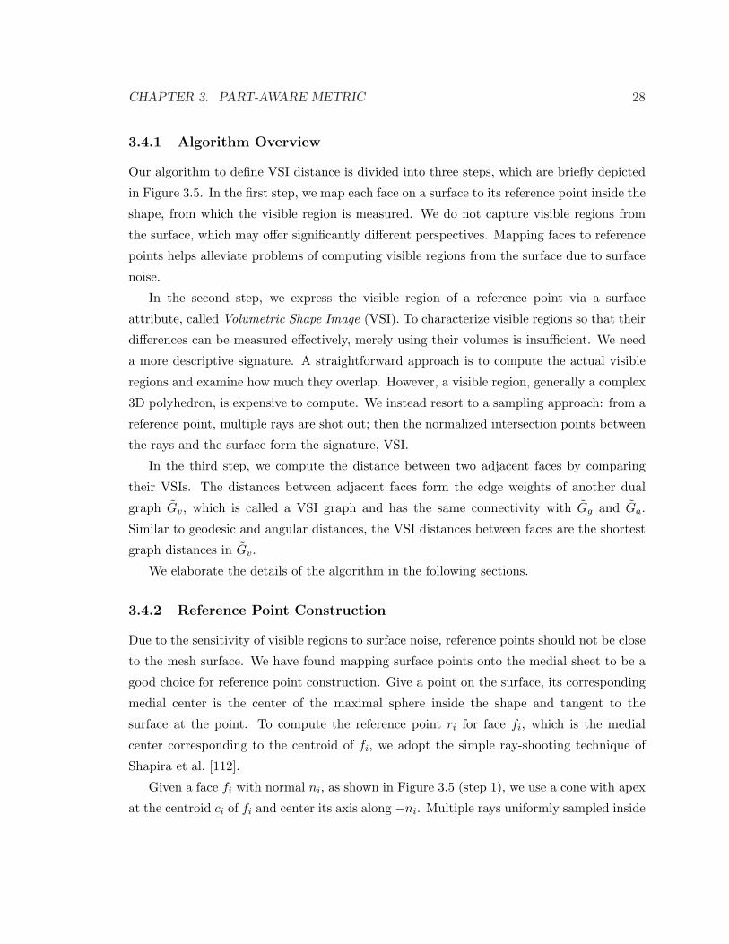
CHAPTER 3. PART-AWARE METRIC 28
3.4.1 Algorithm Overview
Our algorithm to define VSI distance is divided into three steps, which are briefly depicted
in Figure 3.5. In the first step, we map each face on a surface to its reference point inside the
shape, from which the visible region is measured. We do not capture visible regions from
the surface, which may offer significantly different perspectives. Mapping faces to reference
points helps alleviate problems of computing visible regions from the surface due to surface
noise.
In the second step, we express the visible region of a reference point via a surface
attribute, called Volumetric Shape Image (VSI). To characterize visible regions so that their
differences can be measured effectively, merely using their volumes is insufficient. We need
a more descriptive signature. A straightforward approach is to compute the actual visible
regions and examine how much they overlap. However, a visible region, generally a complex
3D polyhedron, is expensive to compute. We instead resort to a sampling approach: from a
reference point, multiple rays are shot out; then the normalized intersection points between
the rays and the surface form the signature, VSI.
In the third step, we compute the distance between two adjacent faces by comparing
their VSIs. The distances between adjacent faces form the edge weights of another dual
graph Gv, which is called a VSI graph and has the same connectivity with Gg and Ga.
Similar to geodesic and angular distances, the VSI distances between faces are the shortest
graph distances in Gv.
We elaborate the details of the algorithm in the following sections.
3.4.2 Reference Point Construction
Due to the sensitivity of visible regions to surface noise, reference points should not be close
to the mesh surface. We have found mapping surface points onto the medial sheet to be a
good choice for reference point construction. Give a point on the surface, its corresponding
medial center is the center of the maximal sphere inside the shape and tangent to the
surface at the point. To compute the reference point ri for face fi, which is the medial
center corresponding to the centroid of fi, we adopt the simple ray-shooting technique of
Shapira et al. [112].
Given a face fi with normal ni, as shown in Figure 3.5 (step 1), we use a cone with apex
at the centroid ci of fi and center its axis along −ni. Multiple rays uniformly sampled inside

CHAPTER 3. PART-AWARE METRIC 29
Figure 3.6: Reference points, shown as blue dots, computed for various models.
the cone, including one along −ni, are cast into the shape. Denote by lj one of the rays,
and ‖lj‖ its length inside the shape. The approximate diameter of the maximal inscribed
sphere touching ci at the surface is
di = argminj‖lj‖/ cos θj,
where θj is the angle between lj and −ni. The reference point ri is the center of that sphere
with radius di/2, namely,
ri = ci − 0.5 ∗ di ∗ ni.
If the local shape is a sphere, all the di’s are equal to its actual diameter. Due to the way
they are constructed, reference points are always inside the shape.
In practice, we set the opening angle of the cone to 80 degrees and cast 16 rays. Note
that if the opening angle is too large, some rays (those with large angles to −ni) may hit the

CHAPTER 3. PART-AWARE METRIC 30
surface immediately after being shot out, making the resulting reference points undesirably
close to the surface. We have found that our setting achieves quality results with high
efficiency. To further improve the robustness of reference points against surface noise and
possible poor tessellation quality, the reference points are subject to a Laplacian smoothing
over a neighborhood graph. The neighborhood graph connects two reference points if their
corresponding faces are adjacent on the mesh, or if the points themselves are close Euclidean
neighbors to each other. In very rare cases, a reference point may move outside the mesh
surface after the smoothing, which can be detected later on and at that time this reference
point is simply moved to its nearest neighbor that stays inside the mesh. Figure 3.6 shows
the reference points computed for four models.
It is worth emphasizing that we only compute the medial points roughly as the reference
points need not strictly reside on medial sheets. Computing rigorous medial sheets [28, 32]
of polygonal shapes is expensive and unnecessary for our purpose.
3.4.3 Volumetric Shape Image (VSI)
We sample the visible regions as seen from the reference points and quantify their differences.
From a reference point ri, we send out m rays uniformly sampled on a Gaussian sphere and
collect the intersection points, s(j)i ’s, between the rays and the surface. Each intersection
point is normalized with respect to its reference point, i.e., s(j)i ← s
(j)i − ri. The normalized
intersection points are stored in a set Si = s(1)i , . . . , s
(m)i , called the volumetric shape
image (VSI) of ri (or of fi). A larger m leads to better approximation of visible regions by
VSIs, but at a higher complexity. We found that setting m = 100 achieves a good trade-off
between accuracy and efficiency. Figure 3.5 (step 2) shows two VSIs, Si (red) of ri and Sj
(green) of rj . To avoid cluttering in the figure, only 8 sampling rays are drawn.
Since the directions of sampling rays are fixed in a global coordinate system, two VSIs are
naturally registered. We may define the difference between two VSIs simply as: diff(Si, Sj) =1m
∑mk=1‖s(k)
i − s(k)j ‖2, which tends to possess large values near boundary regions due to
dramatic visible region changes. Albeit meaningful, such a measure fails to accommodate
accumulated translation errors. Consider a reference point moving within a large part.
Though the slight translation between two adjacent positions generates only a small VSI-
difference, such small differences are easily accumulated up along the way. This can be
observed from the significant difference between Si and Sj , as illustrated in Figure 3.5 (step
2), despite that both ri and rj are within the same part.

CHAPTER 3. PART-AWARE METRIC 31
Figure 3.7: Plot (blue curve) of VSI differences as a point (red dot) moves along the whitecurve on the surface. Visible regions at reference points (blue dots) are in green. (a)-(b):Gradual changes of visible region and VSI (difference ≈ 0) while in the bottom part. (c)-(d):Large change near part boundary. (e): Gradual changes while in the top part.
We have observed that the reach of a local volume along a certain direction, measured
from reference points, is in general more stable. Figure 3.5 (step 3) attests to this obser-
vation, where we see that the reach of the lower part volume along the four directions are
almost the same, though ri and rj are distant. To exploit this property, we pick the m
sampling rays in opposite directions (m/2 ray pairs). Supposing the two intersection points
of a ray pair are stored consecutively in Si, we define the difference between two VSIs as
diff(Si, Sj) =1∑k wk
m/2∑
k=1
wk
(l(k)i − l
(k)j
)2, (3.3)
where l(k) = ‖s(2k−1) − s(2k)‖ is the local reach along the k-th direction. Weights wk’s
are designed to penalize outliers: since VSI is discrete, not all (l(k)i − l
(k)j )2 may faithfully
reflect the difference of the visible regions. To tackle this problem, we fit a Gaussian to the
distribution of such values and set
wk =
e−(dk−u)2/(2σ2) if dk < u + 2σ
0 else dk ≥ u + 2σ, (3.4)

CHAPTER 3. PART-AWARE METRIC 32
where dk = (l(k)i − l
(k)j )2, u is the mean, and σ is the standard deviation. Accordingly, values
are weighted based on their frequencies. Outliers falling two deviations above the mean are
ignored. Figure 3.7 illustrates how diff(·) changes between two adjacent positions when a
point travels on the surface of a simple synthetic “T” shape.
With the edge Gv(i, j) of graph Gv weighted by diff(Si, Sj), VSI distances are simply
the shortest graph distances in Gv. Two VSI distance fields on the snake model are shown
in Figure 3.8. Compared with the geodesic and angular distance fields on the same model
in Figure 3.3, VSI distance stays fairly stable within parts, and induces large jumps across
part boundaries. More comparative results on natural models are provided in Figure 3.9.
Notice how the boundary regions, either between the little finger and the palm, between
the horse’s front leg and the body, or between the dragon’s tail and the body, manifest
significant VSI distance changes. From these examples, we see that VSI distance clearly
outperforms angular distance with respect to encoding part structures.
Two practical Issues Computational-wise, the most expensive part of constructing Gv is
the ray-surface intersection tests required by computing reference points and VSIs. Suppose
an input mesh has n faces, computing reference points and VSIs require 16n and 100n
intersection tests, respectively. To speed up the processing, we voxelize the space using an
axis-aligned grid and assign each mesh face to the voxels it intersects. In our implementation,
we fix the number of voxels to 106. According to the extent of an input mesh along each axis,
the resolution of the grid along an axis is dynamically modified proportionally. During the
ray-surface intersection test, we traverse the voxels along the ray direction for intersection
detection. When an input mesh is dense, we further speed up the processing by computing
VSIs for only a small set of reference points and interpolating for nearby ones. In our
implementation, we compute only 1% of the VSIs and the remaining ones are interpolated.
Therefore the total number of ray-surface intersection tests is 16n + 1% · 100n = 17n.
Also note that although our discussion has assumed closed meshes so far, VSIs can be
computed for open meshes as well, so long as the mesh volume is reasonably well-defined.
This is achieved by simply ignoring rays that do not intersect the surface. The hand model
in Figure 3.9 is an open mesh.

CHAPTER 3. PART-AWARE METRIC 33
Figure 3.8: Two VSI distance fields on the snake model. Red spheres indicate source faces.
(a) hand (b) horse (c) dragon
Figure 3.9: Angular distance fields (top row) vs. VSI (bottom row) distance fields on variousmodels. Red spheres indicate source faces.

CHAPTER 3. PART-AWARE METRIC 34
3.5 Combining Distances
The final part-aware distance we develop is a combination of the geodesic, angular, and VSI
distances. In order to derive the combined distance, we blend the three graphs, Gg, Ga, and
Gv, i.e.,
Gc =(α⊗ Gg
)⊕
(β ⊗ Ga
)⊕
(γ ⊗ Gv
), (3.5)
where α+β +γ = 1 and 0 ≤ α, β, γ ≤ 1. Operator ⊗ multiplies the edge weights of a graph
by a scalar, and ⊕ blends two graphs by summing up the weights of corresponding edges.
The final part-aware metric is defined as the shortest graph distances between the nodes of
Gc. Note that as the three graphs encode different types of information, their edge weights
must be normalized first. To this end, we linearly normalize the edge weights of each graph
to [0, 1].
For the part-aware metric, the parameters, α, β and γ, control the relative importance of
the three distances, and their setting is application-dependent. For example, in structural-
level mesh segmentation, we are primarily interested in a shape’s part structure; therefore
we should emphasize the VSI distance. For shape registration, however, the importance of
geodesic distance ought to be increased, as both the invariance to stretching (merit of VSI
distance) and the invariance to pose (merit of geodesic distance) are desired. Note that the
edge weights in Gg are biased towards 1 after the normalization, since the majority of the
edges or the faces of a mesh typically tend to have similar sizes. However, this is not true
for the edge weights in Ga and Gv. For this reason, α is typically set to a small value in
order for the other two distances to take effect.
3.6 Experimental Results
Complexity Let’s first have a look at the expected asymptotic complexity of constructing
the graph Gc. Given an input mesh M with n faces, constructing the graphs Gg and Ga
involves only local tests and the complexity is O(n). The dominant complexity comes
from building Gv where intersections between rays and surface have to be computed. Let’s
assume that a space partitioning grid is used and the resolution along each dimension is
r. The expected number of voxels traversed before a ray hits a face is at most of O(r).
Our experiments show that typically only about 3% of the voxels are non-empty; so each
non-empty voxel contains about 100n/3r3 faces. As a result, each ray-surface intersection

CHAPTER 3. PART-AWARE METRIC 35
test involves a complexity of O(r + 100n/3r3) in expectation. As per Section 3.4.3, there
are 17n such tests, making the overall complexity to O(17rn + 1700n2/3r3). Though the
theoretical comlexity is quadratic, the constant factor 3r3 (3× 10⁶ in our implementation)
is able to reduce the complexity effectively in practice. If an input mesh is huge, we can
increase the resolution of the grid accordingly. For example, computing VSIs for the dragon
model with 50K faces in Figure 3.6 takes about 15 seconds.
Overview of experiments Although we develop the part-aware metric for mesh seg-
mentation, the metric itself, as a general tool, can be exploited in many other applications
as well. In this section, we conduct several experiments to verify the effectiveness of the
part-aware metric for some non-segmentation applications, including sampling, registration,
and retrieval. We show how this metric is used for segmentation in subsequent chapters.
In the first experiment, our part-aware distance (with emphasis on the VSI distance) is
compared with three existing ones to show how the VSI distance helps capture part infor-
mation. The three distances are the geodesic distance, the geodesic+angular distance [59],
and the diffusion distance studied in [30]. Modeled using random walk, the diffusion dis-
tance measures the overall connectedness between points over the surface. It considers more
global information than the geodesic and angular distances, hence more sensitive to parts
in general. However, it is still purely surface-based and does not account for volumetric
information explicitly. The iso-contour plots in Figure 3.10 clearly show that only our part-
aware metric fully senses the boundary of the bottom part of the “T” shape. This is not
surprising because the VSI difference based on visible region changes is not affected by the
local flatness, as already shown in Figure 3.7.
Part-aware sampling: The max-min sampling scheme can be used for uniform sampling
on a surface. It iteratively places a sample that maximizes the minimum distance, measured
by the geodesic metric, from all previously found samples. Beyond uniform sampling, it is
often desirable to distribute samples based on certain feature criteria. In typical feature-
sensitive remeshing, more samples are placed near high curvature regions, resulting in higher
triangle density therein. This can be accomplished using max-min sampling, but with
the isophotic metric [66]. Figure 3.11(a) shows a feature-sensitive sampling on the pliers
model. When our part-aware metric is applied, the feature regions tend to correspond to
part boundaries, even if a boundary region is locally flat (different from feature-sensitive
sampling). This is shown in Figure 3.11(b). In this test, we set α = 0.01, β = 0, and

CHAPTER 3. PART-AWARE METRIC 36
(a) geodesic (b) diffusion
(c) geodesic+angular (d) part-aware
Figure 3.10: Iso-contours for four distance metrics: 10 contours sampled up to the max-imum distance from the source (red dot). Both geodesic (a) and diffusion (b) distancesare insensitive to the perceived part boundary over the flat region indicated by the arrow.Angular distance (c) senses concavity, but not the part boundary over the flat region. Ourpart-aware metric (d) senses the whole part boundary.

CHAPTER 3. PART-AWARE METRIC 37
(a) (b)
Figure 3.11: Feature-sensitive sampling (a) vs. part-aware sampling (b), where the cyandots indicate the sample vertices. The sampling rate is 10%.
γ = 0.99. We emphasize the VSI distance and ignore the angular distance, so that samples
would not concentrate in concave regions.
A straightforward use of a part-aware surface tessellation is in neighborhood traversal:
a part-aware neighborhood can be traced simply by following topological distances in the
mesh graph. Also, more granularities near part boundaries enable more refined deformation
behavior over those non-rigid regions. In contrast, having large triangles which cut across
part boundaries would be undesirable in this context.
Shape registration: Shape registration or correspondence [21, 53] is another good exam-
ple where a surface metric can become useful. For such a task, bending-invariance is an
important property and it has been successfully addressed [33] by using geodesic distance,
which is insensitive to bending. However, stretch-invariance still remains challenging. In
this experiment, we investigate how our part-aware metric could potentially improve shape
registration. To this end, we consider the spectral correspondence framework [53]. Briefly,
we spectrally embed mesh vertices into a Euclidean space and the registration is established
by corresponding the embeddings using the iterative closest point algorithm [14].
Figure 3.12 shows the derived embeddings of two Homer models. To focus on stretching,
we purposely stretched the left arm and the right leg of one Homer. As stretching changes
the geodesic distance between vertices, the resulting embeddings in (b) and (e) using the

CHAPTER 3. PART-AWARE METRIC 38
(a) Homer (b) geodesic (c) part-aware
(d) stretched (e) geodesic (f) part-aware
(g) registration of (b) and (e) (h) registration of (c) and (f)
Figure 3.12: Spectral embeddings and registration of two Homer models. In the first row,plots (b) and (c) show the embeddings of the original Homer (a) using geodesic and part-aware distances, each of which from two viewing angles. Similarly, the second row is for thestretched Homer (d). The coloring implies the mapping between the original mesh verticesand their embeddings. We see that the embeddings in (c) and (f) are much more similar toeach other than those in (b) and (e) (especially for the feet), thanks to the stretch-invarianceof VSI distances. This helps the subsequent registration operation, whose results are shownin (g) and (h).

CHAPTER 3. PART-AWARE METRIC 39
geodesic distance are quite different. In contrast, the VSI distance is more stable against
stretching. When it is combined with the geodesic distance, the embeddings in (c) and
(f) are made much more similar, facilitating the registration operation in sequel. We set
α = 0.1, γ = 0, and γ = 0.9 and note that this setting places sufficient emphasis on geodesic
distances as per the weight distribution in Gg (see Section 3.5).
In practice, we believe that both geodesic and VSI distances should be considered si-
multaneously for registration, since the former contributes to bending-invariance, while
the latter contributes to stretch-invariance. Also, the geodesic distance imposes certain
distances between neighboring vertices and keeps them adequately spread-out in the em-
bedding. Their weights may be tuned to strike the balance between the two. It is worth
investigating how their weights can be set automatically based on the input data.
Shape retrieval: We also study the potential benefits our metric can offer for shape
retrieval. Osada et al. [91] consider using the probability distribution sampled from a shape
function as a shape descriptor. It is suggested that the D2 shape function, namely the
pairwise Euclidean distances between surface points, serves as a good candidate. Geodesic
distance shape function is investigated in [81]. Although it is invariant to bending, the
probability distribution function of geodesic distances is not sufficiently discriminative in
general. We plan to add more discriminating power to this descriptor, while preserving
sufficient bending-invariance.
In our experiment, we select ten models shown in Figure 3.13. The first five of them
(kangaroo, cat, camel, wolf, and dinopet) are animals with similar part structures, but under
different articulation and stretching. In retrieval, the ideal result should be that when using
each of these five shapes to query, the other four come on top. We consider three shape
functions: geodesic, D2, and our part-aware distances. For each sampled shape function,
we compute its histogram, which serves as the shape descriptor. During retrieval, the χ-
square distances between histograms are used to rank the matches. Figure 3.14 shows the
retrieval results using the three shape functions. We see that only our part-aware metric is
able to consistently achieve the ideal results for all the five similar shapes. Note that in the
last column, we query using the octopus simply for comparison purpose, in which the ideal
ranking is hard to judge.
We set α = 0.02, β = 0, and γ = 0.98, making γ À α to showcase our goal. From Fig-
ure 3.13, we observe that the histograms of geodesic and D2 distances stay relatively stable.
Contrastingly, the part-aware metric produces more discriminating histograms. Meanwhile,

CHAPTER 3. PART-AWARE METRIC 40
kangaroo Geodesic D2 Part−aware
cat
camel
wolf
dinopet
kitten
duck
venus
octopus
T
Figure 3.13: Models used for shape retrieval test and their signature histograms. The lastthree columns show the distance histograms of each model, via geodesic, D2, and part-awaredistances, respectively.

CHAPTER 3. PART-AWARE METRIC 41
Figure 3.14: Retrieval results using geodesic, D2, and part-aware distances. In each block,we run 6 queries and the query shapes sit in the first (shaded) row. In each column, the 4most similar shapes are shown; the non-optimally retrieved shapes are marked by squares.

CHAPTER 3. PART-AWARE METRIC 42
due to the geodesic ingredient in the metric, bending invariance is also preserved to a cer-
tain extent; this is exemplified by the similarity among the first four histograms in the last
column. This experiment highlights an advantage of our metric: by combining geodesic
distance and VSI distance, it provides an effective compromise between bending-invariance
and discriminating capability. However, this is a rather preliminary test and it is worth
expanding the database and investigating more in this issue.
3.7 Summary
A part-aware metric, as a fundamental tool, is not only useful for mesh segmentation, but
also of general interest to a variety of geometry analysis and processing tasks. Although
isophotic [66] and diffusion [30] distances have been successfully applied to mesh segmenta-
tion, the distances themselves do not explicitly take part information into consideration.
In this chapter, we develop a part-aware surface metric specifically for encoding part
information. The metric combines three components: geodesic, angular, and VSI distances.
Our key observation is that the visible region, of a point inside the shape volume, is sensi-
tive to part boundaries. Such a property is realized into the VSI distance which effectively
captures part information, while geodesic and angular distances complement the VSI dis-
tance. We compare our metric against existing ones and also apply it to several part-related
applications, including shape registration, part-aware sampling, and shape retrieval. The
effectiveness of our metric is testified empirically. We make use of this metric for mesh
segmentation in the following chapters.

Chapter 4
Segmentation using Spectral
Clustering
4.1 Overview
Using the part-aware metric from Chapter 3, we develop a k-way mesh segmentation algo-
rithm based on spectral clustering in this chapter. Figure 4.1 gives the flow of the algorithm.
input : Mesh M, the number of segments k.output: Sub-meshes O = M1,M2, ...,Mk.begin
U ← ComputeEmbedding(M) ; /* Section 4.2 */O =← Kmeans(M, U , k) ; /* Section 4.3 */
end
Figure 4.1: Mesh segmentation based on spectral clustering.
Given an input meshM and an intended number of segments k from a user, the algorithm
first constructs a spectral embedding U (Section 4.2) for the faces of M, using the part-
aware metric. We study our spectral embedding algorithm along with several related issues
in the light of kernel principal component analysis. With the embedding U at hand, the
classical K-means clustering algorithm is readily applied to obtain the segmentation result
(Section 4.3). Several questions associated with K-means are also addressed. Experimental
results and summary are presented in the last two sections.
43

CHAPTER 4. SEGMENTATION USING SPECTRAL CLUSTERING 44
4.2 Construction of Spectral Embedding
The spectral embedding for the faces of the input mesh M is derived from their distances
prescribed by the part-aware metric using the algorithm presented in Figure 4.2. There
are many spectral embedding algorithms and they all have their own pros and cons. Our
embedding algorithm is designed specifically for mesh segmentation, and it is analyzed in
the light of kernel principal component analysis [109]. We also address several practical
issues that are critical to the effectiveness of the algorithm.
1. Compute a distance matrix G and convert it to an affinity matrix W , whereWij = e−Gij/2σ2
and σ is set to the square root of the average of the entries of G.
2. Compute the eigenvalue decomposition W = V ΛV T .
3. Let Λ = diag(λ1, λ2, . . . , λn) and λ1 ≥ λ2 ≥ . . . ≥ λn. Supposing λr, 1 ≤ r ≤ n, is thesmallest positive eigenvalue, set Λ′ = diag(λ2, λ3, . . . , λr), ignoring the largesteigenvalue.
4. Set U = V[2...r]Λ′12 , where V[2...r] is the sub-block of U from the second column to the
r-th column, inclusive. Then Ui· (the i-th row of U) is the embedding, denoted byfe
i , of face fi. We denote Fe = fei .
Figure 4.2: Spectral embedding of mesh faces.
Through this algorithm, the mesh faces are embedded in Euclidean space to facilitate
the subsequent clustering operation. Clearly, W encodes the similarities between faces —
Wij is inversely (exponentially) proportional to Gij and recall that Gij is the part-aware
distance between faces fi and fj . In Section 4.2.6, we show that the distance between two
embedded faces, fei and fe
j , is approximately√
2− 2e−Gij/2σ2 . This implies that if a pair
of faces have a large part-aware distance, then their distance in the embedding space is also
large. Such a property is the premise for the success of our segmentation algorithm. In the
following sections, we study the details of this spectral embedding algorithm.
4.2.1 Affinities
In Section 3.5, we have defined the part-aware distance using the combined graph Gc: the
distance between two faces is the shortest graph distance between their corresponding nodes
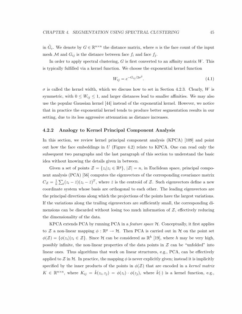
CHAPTER 4. SEGMENTATION USING SPECTRAL CLUSTERING 45
in Gc. We denote by G ∈ Rn×n the distance matrix, where n is the face count of the input
mesh M and Gij is the distance between face fi and face fj .
In order to apply spectral clustering, G is first converted to an affinity matrix W . This
is typically fulfilled via a kernel function. We choose the exponential kernel function
Wij = e−Gij/2σ2. (4.1)
σ is called the kernel width, which we discuss how to set in Section 4.2.3. Clearly, W is
symmetric, with 0 ≤ Wij ≤ 1, and larger distances lead to smaller affinities. We may also
use the popular Gaussian kernel [44] instead of the exponential kernel. However, we notice
that in practice the exponential kernel tends to produce better segmentation results in our
setting, due to its less aggressive attenuation as distance increases.
4.2.2 Analogy to Kernel Principal Component Analysis
In this section, we review kernel principal component analysis (KPCA) [109] and point
out how the face embeddings in U (Figure 4.2) relate to KPCA. One can read only the
subsequent two paragraphs and the last paragraph of this section to understand the basic
idea without knowing the details given in between.
Given a set of points Z = zi|zi ∈ Rg, |Z| = n, in Euclidean space, principal compo-
nent analysis (PCA) [56] computes the eigenvectors of the corresponding covariance matrix
CZ = 1n
∑i(zi − z)(zi − z)T , where z is the centroid of Z. Such eigenvectors define a new
coordinate system whose basis are orthogonal to each other. The leading eigenvectors are
the principal directions along which the projections of the points have the largest variations.
If the variations along the trailing eigenvectors are sufficiently small, the corresponding di-
mensions can be discarded without losing too much information of Z, effectively reducing
the dimensionality of the data.
KPCA extends PCA by running PCA in a feature space H. Conceptually, it first applies
to Z a non-linear mapping φ : Rg → H. Then PCA is carried out in H on the point set
φ(Z) = φ(zi)|zi ∈ Z. Since H can be considered as Rh [19], where h may be very high,
possibly infinite, the non-linear properties of the data points in Z can be “unfolded” into
linear ones. Thus algorithms that work on linear structures, e.g., PCA, can be effectively
applied to Z inH. In practice, the mapping φ is never explicitly given; instead it is implicitly
specified by the inner products of the points in φ(Z) that are encoded in a kernel matrix
K ∈ Rn×n, where Kij = k(zi, zj) = φ(zi) · φ(zj), where k(·) is a kernel function, e.g.,

CHAPTER 4. SEGMENTATION USING SPECTRAL CLUSTERING 46
a Gaussian. Then computations in H based only on inner products of the data can be
efficiently implemented in the original space by replacing inner products with the kernel
function k(·).We now review how KPCA is performed. Denoting by Φ = [φ(z1)|φ(z2)|, . . . , |φ(zn)],
then the covariance matrix of φ(Z), ignoring the normalization by 1n , is
Cφ(Z) = ΦΦT =n∑
i=1
φ(zi)φ(zi)T . (4.2)
Note that we assume for now that φ(Z) is already centered. For the simplicity of notation,
in the following we denote φ(zi) by ϕi. As we are interested in the eigenvectors of Cφ(Z),
we write
ρmHm = Cφ(Z)Hm =n∑
i=1
(ϕTi Hm)ϕi, (4.3)
where ρm ≥ 0 is the m-th largest eigenvalue and Hm ∈ H \ 0 is the corresponding
eigenvector. Notice that although ϕi may have infinite dimensionality, Cφ(Z) can have at
most n positive eigenvalues as there are only n points. From this equation, we see that the
principal component Hm can be represented by a linear combination of ϕj ,
Hm =n∑
j=1
ξ(j)ϕj , (4.4)
with ξ(j) standing for the j-th entry of the coefficient vector ξ. This is an important
observation. If we plug Hm into Equation 4.3 and left-multiply both sides by ϕT (ϕ ∈ φ(Z)),
it yields
ρm
n∑
j=1
ξ(j)(ϕ · ϕj) =n∑
j=1
ξ(j)(ϕj ·
n∑
i=1
ϕi
)(ϕ · ϕj), (4.5)
or in matrix form
ρmKξ = K2ξ. (4.6)
Since K is symmetric and positive semidefinite, Equation 4.6 is equivalent to
ρmξ = Kξ, (4.7)
from which we see that ξ is simply an eigenvector of K. Let µ1 ≥ . . . ≥ µm ≥ . . . ≥ µn ≥ 0
be the eigenvalues of K and Ξ = [Ξ1|Ξ2| . . . |Ξn] contains the corresponding eigenvectors, we
have Hm =∑
j Ξ(j)m ϕj from Equation 4.4. Intuitively, the entries of Ξm are the coefficients

CHAPTER 4. SEGMENTATION USING SPECTRAL CLUSTERING 47
of the linear combination of ϕj ’s that represents the m-th principal component, Hm, of
φ(Z). Therefore the projection of any point ϕi on Hm is
Hm · ϕi =( n∑
j
Ξ(j)m ϕj
) · ϕi =n∑
j
Ξ(j)m (ϕj · ϕi) =
n∑
j
Ξ(j)m Kji = KT
·i Ξm = Ki·Ξm, (4.8)
with K·i and Ki· being the i-th column and i-th row of K, respectively. If we require Hm
to be normalized, it implies
1 = Hm ·Hm =n∑
j
Ξ(j)m ϕj ·
n∑
j
Ξ(j)m ϕj =
n∑
i,j=1
Ξ(i)m Ξ(j)
m (ϕi · ϕj) = Ξm ·KΞm = µm(Ξm · Ξm).
(4.9)
Therefore we should normalize Ξm ← Ξm/√
µm and Equation 4.8 translates into
Hm · ϕi = Ki·Ξm/√
µm = (µmΞm)i/√
µm =√
µmΞ(i)m . (4.10)
Based on all above discussions, we are able to draw the similarity between KPCA and
spectral embedding, which has been previously noted in [13]. Assuming that the affinity
matrix W has only non-negative eigenvalues, we denote its eigenvalue decomposition by
W = V ΛV T and set U ′ = V Λ12 , namely,
U ′im =
√λmV (i)
m . (4.11)
Notice that the right sides of Equations 4.10 and 4.11 take the same form. Therefore,
if we consider W as the kernel matrix K, for the points in H induced by W , U ′im can
be viewed as the projection of the i-th point onto the m-th principal component. More
specifically, if we assume (a) the points in the feature space H induced by W are centered,
and (b) W is positive semidefinite (since W is symmetric, this implies that all its eigenvalues
are non-negative), the rows of U ′ are essentially the embeddings via KPCA induced by
W . Unfortunately, the above two conditions are not guaranteed for the affinity matrix W
produced in the first step of our algorithm in Figure 4.2. However, we show in Section 4.2.4
and Section 4.2.5 how our face embeddings in U (Figure 4.2) have already implicitly met
these two conditions. Let’s recapitulate the property of the embeddings in U in the following
observation:
Observation 4.1. The affinity matrix W induces n points in a high dimensional feature
space H. Ui· (the i-th row of U) are the embedded coordinates for face fi in the coordinate
system whose basis are the principal components of the induced points in H.

CHAPTER 4. SEGMENTATION USING SPECTRAL CLUSTERING 48
4.2.3 Kernel Width
The kernel width σ in Equation 4.1 plays an important role in spectral clustering. Au-
tomatically setting σ to achieve robust clustering results against all kinds of input data
is challenging and manual tuning is typically required, although automatic methods ex-
ist [37, 83]. We do not intend to solve this problem in general; instead, we simply find a
way to set σ to suit mesh segmentation in our application.
(a) enforcer model
0 0.5 1 1.5 2 2.50
0.2
0.4
0.6
0.8
1
Gij
Wij
=e−
Gij/2σ
2
σ = 0.15
σ = 0.69
σ = 2.62
(b) kernel functions with different σ
Figure 4.3: Exponential kernel functions with different kernel widths tested on the enforcermodel with 600 faces.
Take the model shown in Figure 4.3(a) for example. We compute the distance matrix
G for its faces. The average and maximum distances are 0.48 and 2.62, respectively. We
plot in Figure 4.3(b) three kernel functions with different kernel widths. From plot (b),
we see that if σ is too large (σ = 2.62, the maximum distance), Wij ’s are squeezed into
a narrow band near 1, sacrificing the contrast between different distances. In the extreme
case, if σ = ∞, W = 11T and all the embeddings reduce to a single point. On the other
hand, if σ is too small (σ = 0.15), Wij vanishes too quickly, making all faces far apart in
the embedding space unless they are sufficiently close on the surface. When σ = 0, W turns
into an identity matrix, in which case all the embeddings in H are equally far away from
each other.
Either too small or too large, σ produces a face embedding with undesirable distribution,

CHAPTER 4. SEGMENTATION USING SPECTRAL CLUSTERING 49
imperiling the segmentation quality. We choose to set σ based on the average distance which
provides a good clue for the right scale of σ. More specifically, we set σ to the square root
of the average distance in G. For example, the green curve (σ = 0.69) in plot (b) depicts
the kernel function when σ is set in such a way. This way, the function spans the range of
affinity values in a more meaningful manner: the changes of Gij gradually contribute less
changes to Wij as Gij increases. We have found that such a mapping works well for our
application in general.
4.2.4 Affinity Matrix Centering
In Section 4.2.2, one of our assumptions made for W is that the induced point set φ(Z)
in H is already centered. In practice, however, this assumption does not normally hold.
Note also that since the coordinates of φ(Z) are unknown, it is impossible to center them
explicitly. Fortunately, it is shown by Scholkopf et al. [109] that the centering can be
implicitly implemented by converting W to W :
W = (I − 1n11T )W (I − 1
n11T ). (4.12)
The major drawback of computing W is the high computational cost when the size of W
is large. As we will see in Chapter 5, the full W is also not available for centering due
to sub-sampling, which is necessary for handling large meshes. In practice, we make the
following observation:
Observation 4.2. Provided that the kernel width σ is sufficiently large, the eigenvalues
and eigenvectors of W well approximate, with a shift, those of W . Specifically, suppose
λ1 ≥ λ2 ≥ . . . are the eigenvalues of W and V1, V2, . . . are the corresponding eigenvectors;
λ1 ≥ λ2 ≥ . . . are the eigenvalues of W and V1, V2, . . . are the corresponding eigenvectors,
we have λ2 ≈ λ1, λ3 ≈ λ2, . . . and V2 ≈ V1, V3 ≈ V2, . . ..
This observation enables us to avoid the centering operation; we can simply ignore the
largest eigenvector of W and use the subsequent eigenvectors. We provide an explanation
and an experiment to attest to this observation.
Since Wij = φ(zi)T φ(zj) and Wii = 1, each φ(zi) has unit length in the feature space and
Wij is simply the cosine of the angle between vectors φ(zi) and φ(zj). Geometrically, this
implies that given any vector φ(zi), ∀j 6= i, φ(zj) lies inside a cone, which is rooted at the
origin with an opening angle of 2θi and its axis along vector φ(zi), where θi is determined

CHAPTER 4. SEGMENTATION USING SPECTRAL CLUSTERING 50
Figure 4.4: Distribution of affinity-implied points in feature space.
by the smallest entry Wit of the i-th row of W . If σ is sufficiently large (see Equation 4.1),
Wit is close to 1 and, accordingly, θi is small. Such a configuration is depicted in Figure 4.4.
Each point φ(zi) is associated with a cone and the intersection of these cones gives a region,
R, in which all the points lie. In the figure, R is the shaded region enclosed by the dashed
curve. Note that the cone and the region R are enlarged for illustration purpose. If φ(Z)
were centered, the region R would have moved to the place indicated by R.
We show that the principal components of the points in R are approximately the same
as the principal components of the points in R, only shifted by one position. Recall that
Cφ(Z) (Equation 4.2) is the covariance matrix of φ(Z). Note that now the points are not
centered yet. The largest eigenvector e1 of Cφ(Z) is the vector p that maximizes the term∑
i ||pT φ(zi)||2. Since all φ(zi)’s have unit length and small angles between each other
(suppose σ is sufficiently large), the region R is small and the distance from any point inside
R to the origin is about 1. So, e1 is roughly a constant vector pointing from the origin
toward the centroid of R to maximize the variance, as illustrated in Figure 4.4. With the
same reasoning, R is “thin” along the direction of e1. Consequently, the space spanned by
φ(Z) is close to the null space of e1. The subsequent eigenvectors e2, e3, . . . of Cφ(Z),
in the null space of e1, are then a good approximation to the principal components which
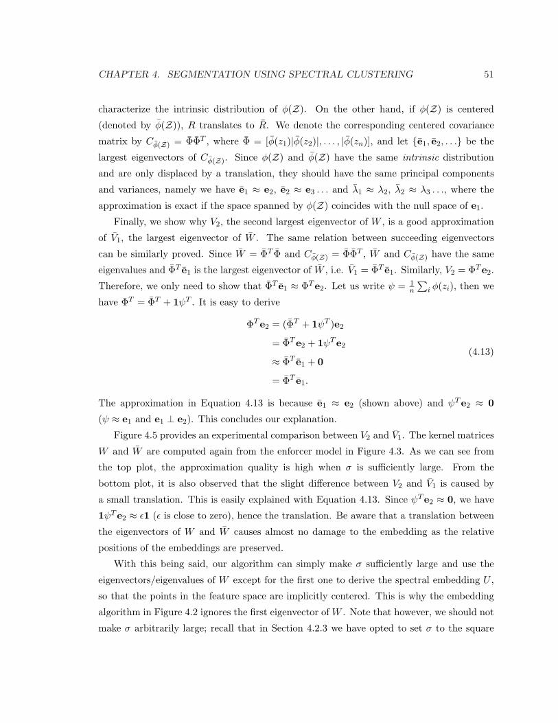
CHAPTER 4. SEGMENTATION USING SPECTRAL CLUSTERING 51
characterize the intrinsic distribution of φ(Z). On the other hand, if φ(Z) is centered
(denoted by φ(Z)), R translates to R. We denote the corresponding centered covariance
matrix by Cφ(Z) = ΦΦT , where Φ = [φ(z1)|φ(z2)|, . . . , |φ(zn)], and let e1, e2, . . . be the
largest eigenvectors of Cφ(Z). Since φ(Z) and φ(Z) have the same intrinsic distribution
and are only displaced by a translation, they should have the same principal components
and variances, namely we have e1 ≈ e2, e2 ≈ e3 . . . and λ1 ≈ λ2, λ2 ≈ λ3 . . ., where the
approximation is exact if the space spanned by φ(Z) coincides with the null space of e1.
Finally, we show why V2, the second largest eigenvector of W , is a good approximation
of V1, the largest eigenvector of W . The same relation between succeeding eigenvectors
can be similarly proved. Since W = ΦT Φ and Cφ(Z) = ΦΦT , W and Cφ(Z) have the same
eigenvalues and ΦT e1 is the largest eigenvector of W , i.e. V1 = ΦT e1. Similarly, V2 = ΦTe2.
Therefore, we only need to show that ΦT e1 ≈ ΦTe2. Let us write ψ = 1n
∑i φ(zi), then we
have ΦT = ΦT + 1ψT . It is easy to derive
ΦTe2 = (ΦT + 1ψT )e2
= ΦTe2 + 1ψTe2
≈ ΦT e1 + 0
= ΦT e1.
(4.13)
The approximation in Equation 4.13 is because e1 ≈ e2 (shown above) and ψTe2 ≈ 0
(ψ ≈ e1 and e1 ⊥ e2). This concludes our explanation.
Figure 4.5 provides an experimental comparison between V2 and V1. The kernel matrices
W and W are computed again from the enforcer model in Figure 4.3. As we can see from
the top plot, the approximation quality is high when σ is sufficiently large. From the
bottom plot, it is also observed that the slight difference between V2 and V1 is caused by
a small translation. This is easily explained with Equation 4.13. Since ψTe2 ≈ 0, we have
1ψTe2 ≈ ε1 (ε is close to zero), hence the translation. Be aware that a translation between
the eigenvectors of W and W causes almost no damage to the embedding as the relative
positions of the embeddings are preserved.
With this being said, our algorithm can simply make σ sufficiently large and use the
eigenvectors/eigenvalues of W except for the first one to derive the spectral embedding U ,
so that the points in the feature space are implicitly centered. This is why the embedding
algorithm in Figure 4.2 ignores the first eigenvector of W . Note that however, we should not
make σ arbitrarily large; recall that in Section 4.2.3 we have opted to set σ to the square

CHAPTER 4. SEGMENTATION USING SPECTRAL CLUSTERING 52
0 0.5 1 1.5 2 2.50
0.2
0.4
0.6
0.8
1
1.2
1.4
σ
||V
1−
V2||
← σ = 0.69
0 100 200 300 400 500 600−0.04
−0.02
0
0.02
0.04
0.06
0.08
0.1
index of eigenvector entries
valu
e of
eig
enve
ctor
ent
ries
V2
V1
Figure 4.5: Influence of kernel width to the approximation quality for V2 and V1. Thetop plot shows that ||V1 − V2|| decreases quickly while the kernel width σ increases, whereσ = 0.69 is the square root of the average distance in G. The bottom plot shows the twoeigenvectors when σ = 0.69, where ||V1−V2|| = 0.15, λ1 = 90.27 (the first eigenvalue of W ),and λ2 = 88.15 (the second eigenvalue of W ). We see that λ1 ≈ λ2 and V1 ≈ V2.

CHAPTER 4. SEGMENTATION USING SPECTRAL CLUSTERING 53
root of the average distance. Practically this is sufficiently large for the purpose of avoiding
centering W , which has been verified by the empirical example from Figure 4.5.
4.2.5 Positive-Semidefiniteness
In Section 4.2.2, we have also assumed that W is positive semidefinite in order for the
KPCA analogy to apply. This is because the kernel matrix K must be positive semidefinite,
which is necessary to derive Equation 4.7 and Equation 4.10. This requirement can be
explained from another perspective as well. Recall that K = ΦT Φ and Cφ(Z) = ΦΦT .
Cφ(Z) is positive semidefinite, since given any vector x ∈ H, xT Cφ(Z)x = xT ΦΦT x =
(ΦT x)T (ΦT x) = ‖ΦT x‖2 ≥ 0. In addition, it is easy to prove that K and Cφ(Z) have the
same eigenvalues1. Therefore K is positive semidefinite.
In reality, however, the W we derive is not guaranteed to be positive semidefinite. The-
oretically speaking, we can deal with this problem by converting W to W which is positive
semidefinite. Let W = V ΛV T be the eigenvalue decomposition, we can also write it as
W =n∑
i=1
λiViVTi , (4.14)
where λi is the i-th largest eigenvalue and Vi is the corresponding eigenvector. Supposing
only the leading r eigenvalues, λ1, . . . , λr, are greater than 0, we set
W =r∑
i=1
λiViVTi , (4.15)
which is obviously positive semidefinite. As we are essentially interested in the eigenvalues
and eigenvectors of W , we may simply take the positive eigenvalues of W and their eigen-
vectors to derive the face embeddings without constructing W explicitly. This is reflected
in the embedding algorithm in Figure 4.2.
With this approach, we need to make sure that not too much information is lost by
discarding the negative eigenvalues and eigenvectors. It is well known in numerical linear
algebra that for a symmetric matrix M with eigenvalue decomposition M =∑n
i=1 λiViVTi ,
where the λi’s are the eigenvalues sorted in descending order by their magnitude and Vi’s
are the respective eigenvectors, the best rank r matrix approximating M (in the sense of
1For any eigenvalue λ and the corresponding eigenvector v of K, λ and Φv are an eigenvalue and thecorresponding eigenvector of Cφ(Z).

CHAPTER 4. SEGMENTATION USING SPECTRAL CLUSTERING 54
the Frobenius norm) is∑r
i=1 λiViVTi . Comparing Equation 4.14 with Equation 4.15, we see
that if W has only a few negative eigenvalues with relatively small magnitudes, only a small
amount of information will be lost when converting W to W .
Empirically, the affinity matrix W we produce from the distance matrix G via an expo-
nential kernel is either positive semidefinite or sufficiently close to be, in the sense that the
number of negative eigenvalues of W is relatively small and their magnitudes are negligible
compared with those of positive eigenvalues. Again let’s take the enforcer model as an ex-
ample, for which W is obtained with the kernel width σ = 0.69. The eigenvalues of W are
88.15, 75.29, 37.65, 26.40, 6.73, . . . , 0, . . . ,−0.029,−0.034; the largest eigenvalue is ignored as
W is not centered (see Section 4.2.4). Only 16% of the eigenvalues are negative, which share
about 0.15% of the energy of the entire spectrum.
4.2.6 Distance between Embeddings
Let’s examine how distances between embedded faces relate to their affinities. Since W in
Equation 4.15 is strictly positive semidefinite and centering inH does not affect the distances
between embedded faces, we can compute the distance between any two embedded faces
φ(fi) and φ(fj) in H as
||φ(fi)− φ(fj)|| =√(
φ(fi)− φ(fj))T (
φ(fi)− φ(fj))
=√
φ(fi)T φ(fi) + φ(fj)T φ(fj)− 2φ(fi)T φ(fj)
=√
Wii + Wjj − 2Wij
≈ √Wii + Wjj − 2Wij
=√
1 + 1− 2Wij
=√
2− 2e−Gij/2σ2,
(4.16)
where the approximation step is due to the fact that W is close to be positive semidefinite
as discussed in Section 4.2.5. Through this equation, we observe that the distances between
embedded faces are exponentially proportional to their distances in G, and the rank order of
distances is preserved as well. Since Ui· (Figure 4.2) is the dimensionality-reduced embedding
of φ(fi) in H via PCA and PCA embedding does not change the distances between entities,
we have
‖Ui· − Uj·‖ ≈√
2− 2e−Gij/2σ2. (4.17)

CHAPTER 4. SEGMENTATION USING SPECTRAL CLUSTERING 55
We also take the enforcer model to verify Equation 4.17 empirically. To this end, we
denote deij = ‖Ui·−Uj·‖ and dHij =
√2− 2e−Gij/2σ2 . For any faces fi and fj , the discrepancy
between deij and dHij is defined as 2|de
ij − dHij |/(deij + dHij ). Then the average discrepancy over
all pairs of faces gives a quantitative estimation about the accuracy of Equation 4.17. For
the enforcer model, the average discrepancy is only 1.23%.
4.2.7 Further Discussions
Our spectral embedding algorithm serves to transform the distances encoded in G to Eu-
clidean embeddings of mesh faces for the subsequent K-means clustering operation. The-
oretically, it is possible to run a K-means algorithm simply based on G without explicit
embeddings, for example, using the method from [59]. Nonetheless, such a method is inef-
ficient and all the entries of G have to be known. When the size of a mesh is large, even
computing the entire G itself is already not affordable. In such cases, we show (Chapter 5)
how to use only a few rows of G to derive face embeddings. With an Euclidean embedding,
K-means can be performed efficiently.
The distances between embedded faces are approximately√
2− 2e−Gij/2σ2 . A large
Gij induces a large embedding distance and vice versa. Note that this distance relation
is monotone and non-linear. By setting the kernel width σ and using the eigenvectors
appropriately, such a distance relation is accurately enforced by our embedding algorithm. In
other words, all the distances encoded in G are consistently reconstructed in the embedding
space governed by this relation. Also, the contrast of the distances in G is well preserved
(see Section 4.2.3); this is important for achieving high quality segmentation results. On the
other hand, if we apply the metric Multi-Dimensional Scaling [27] based on G to derive face
embeddings, inferior segmentation results are shown by our experiments. This is because
G in general has relatively large negative eigenvalues, which defies the positive semidefinite
requirement in order for MDS to apply meaningfully.
4.3 K-means Clustering
So far, we have obtained the spectral embedding Fe = fei n
i=1 for the faces of the input mesh
M. The embedding coordinate for face fi is denoted by fei = Ui·, and the dimensionality is
at most n− 1, which is achieved when W is positive definite (note that we discard the first
eigenvalue/eigenvector). In the embedding space, the face distances reflect the part-aware

CHAPTER 4. SEGMENTATION USING SPECTRAL CLUSTERING 56
1. Assuming k ≤ r − 1, reduce the dimensionality of Fe by keeping only the first kcolumns of U . Recall that r is the number of positive eigenvalues of W (Figure 4.2).
2. Initiate a proxy set P = piki=1, where P ⊂ Fe. Each pi represents cluster Fe
i andall pi’s are mutually farthest apart in the embedding space.
3. Element assignment : for each fe, assign it to the cluster Fei , where
i = argmin1≤j≤k‖fe − pj‖. Namely, a face is assigned to the closest proxy.
4. Proxy fitting : refine each proxy pi to the centroid of cluster Fei .
5. Repeat step 3 and step 4 until P is stable.
Figure 4.6: K-means clustering in embedding space.
distances in G. The next step is to apply K-means clustering to Fe to obtain the actual
segmentation result.
The general framework of a K-means algorithm has been briefed in Section 2.2.1 when
variational segmentation approaches are discussed. We formally describe the K-means al-
gorithm for our application in the following.
Given the face embedding Fe, we seek a clustering Θ = Fei k
i=1, where⋃k
i=1Fei = Fe
and Fei
⋂Fej,j 6=i = ∅, such that the cost function
cost(Fe
i ki=1
)=
k∑
i=1
( ∑
fej ∈Fe
i
‖fej − Fe
i ‖)
(4.18)
is minimized, where k is the number of segments given by a user and Fei is the centroid of
cluster Fei . The term in the bracket on the right side of the equation measures the intra-
cluster cost. If every embedding is close to the centroid of its cluster, the cluster is tight
and the intra-cluster cost is low. Figure 4.6 demonstrates how the K-means is performed in
our algorithm. Intuitively, the algorithm finds an approximate solution (a local minimum)
to Equation 4.18 by iteratively reducing intra-cluster costs. In each iteration, a face is
assigned to its closest proxy and each proxy is refined to its cluster centroid. These two
steps alternate until all the proxies are stable, implying that a local minimum is reached.
When the K-means algorithm converges, each cluster Fei is tight and the distances
between the centroids of different clusters are large. Such clusters are likely to correspond
to the parts of the input mesh M.

CHAPTER 4. SEGMENTATION USING SPECTRAL CLUSTERING 57
4.3.1 Dimensionality Reduction
The initial embedding of Fe, derived as in Figure 4.2, has a dimensionality of at most n−1.
As discussed in Section 4.2.5, we may discard those dimensions whose corresponding eigen-
values are non-positive. However, the resulting dimensionality could still be high, especially
when n is large. High embedding dimensionality poses two computational bottlenecks: one
for the eigenvalue decomposition of W and the other for the K-means clustering.
We reduce the dimensionality of an embedding by dropping the trailing columns of
U . According to the analogy to KPCA, this is equivalent to the standard dimensionality
reduction via PCA, but carried out in the feature space H. In practice, the embedding
dimensionality is reduced rather aggressively — we only keep the first k columns of U .
The benefits are twofold. First, as k is typically small (less than 15 as a model usually
does not contain too many parts), we only need to compute the first k + 1 eigenvectors of
W . This can be efficiently carried out using the ARPACK [70] package, which is designed
to solve large scale eigenvalue problems with capability to compute only leading or trailing
eigenvectors. Secondly, discarding the trailing eigenvectors helps get rid of high “frequency”
information. This means that the resulting embeddings would attempt to preserve only the
distances between prominent clusters, while the distances between intra-cluster points are
ignored. This makes the K-means algorithm work more favorably to extract prominent
clusters without being distracted by intra-cluster distances.
4.3.2 Proxy Initialization
Our K-means algorithm is subject to local minima, and the clustering result has much to
do with the seed proxy set P. Although finding the global optimum for a K-means problem
is known to be NP-hard, it is possible to apply certain heuristics to improve the clustering
quality. One simple way is to run K-means with random initial proxies for multiple times
and choose the result for which Equation 4.18 is minimized. Another way is to randomly
select a subset of the original data, run K-means on the selected data, and utilize the
preliminary clustering result to initialize the proxies for the final clustering performed on
the full data.
However, both methods do not make full use of the information encoded in the embed-
ding. Since we want the resulting clusters to correspond to the mesh parts, it is natural to
pick a seed proxy from each part. As our part-aware metric imposes large distances between

CHAPTER 4. SEGMENTATION USING SPECTRAL CLUSTERING 58
parts and the distances are well preserved in the embedding space, it implies that the seed
proxies are likely to be mutually far apart. Therefore, we adopt a max-min scheme to find
such proxies. We select the first two proxies that are farthest away in the embedding space.
Then each subsequent proxy is inserted such that it maximizes the smallest distance to the
previously chosen proxies. We have found that such a scheme effectively alleviates the local
minima problem of our K-means algorithm.
4.3.3 Boundary Enhancement
Nearby faces on a mesh face should be close in the embedding space because we derive
distances in G as graph distances, which are continuous. However, faces in each cluster
output by the K-means algorithm are not guaranteed to form a single connected region
(referred to as a component in this context) on a mesh surface, although in practice they
often do. Rarely, few faces along a part boundary might be disconnected from the core
region. The boundaries between the parts could also present some local artifacts, including
jaggedness or slight deviation from the intended boundary positions. We fix such problems
in a post-processing stage.
We adopt a functional optimization framework that considers spatial coherence. This
idea is developed by Boykov et al. [17] and used for meshes [112]. Recall that Θ is the
clustering result from the K-means algorithm. It can also be considered as a labeling of
faces with respect to the converged proxies. Let’s denote the converged proxies by P ′. Our
goal is then to come up with a refined clustering/labeling Θ′ with respect to P ′ such that
the following functional is minimized:
E(Θ′) = Edata(Θ′) + µEsmooth(Θ′). (4.19)
Edata(Θ′) is designed to respect Θ, and Esmooth(Θ′), weighted by µ, is used to enhance part
boundaries.
Given a face fi, suppose it is labeled pfi in Θ′, where pfi ∈ P ′. We define function
h1(fi, pfi) = − log
(1/d(fi, pfi)∑k
j=1
(1/d(fi, pfj
)))
,
where d(·) denotes the Euclidean distance between the embedding of a face and a proxy.
Intuitively, h1(·) ∈ (0, +∞) measures how “bad” it is if fi is clustered to pfi . Specifically, if
fi’s embedding, fei , is actually closest to pfi after our K-means clustering, h1(fi, pfi) would

CHAPTER 4. SEGMENTATION USING SPECTRAL CLUSTERING 59
be small and vice versa. We define Edata(Θ′) =∑n
i=1 h1(fi, pfi); therefore minimizing Edata
means to honor the overall result from the previous K-means clustering.
The smooth term is defined as Esmooth(Θ′) =∑
(fi,fj)∈N h2(fi, fj , pfi , pfi), where N is
the set of pairs of adjacent faces (sharing a common edge). Esmooth(Θ′) is a measure about
part boundaries, providing h2(·) does not vanish only when pfi 6= pfj . Specifically, we define
h2(fi, fj , pfi , pfi) =
l(eij)(1− weight(eij)
)pfi
6= pfj
0 pfi = pfj
,
where l(eij) is the length of the common edge eij of fi and fj , normalized by the maximum
edge length over the entire mesh surface, and weight(eij) is the mapped angular weight
(Section 3.3) of eij , defined as
weight(eij) = log(νGa(i, j) + 1
)/ log(ν + 1). (4.20)
Via this logarithmic mapping [112], with ν controlling the mapping strength, the influences
of small angular weights are enhanced. Such a mapping helps improve the boundary qual-
ity in our experiments. Intuitively, minimizing Esmooth(Θ′) implies to favor a short part
boundary consisting of concave edges. In our application, we set µ = 0.3 and ν = 10.
Equation 4.19 is minimized approximately via a minimum graph cut problem [17]. By
subjecting Θ to such a smoothing procedure, the refined clustering Θ′ induces short bound-
aries across concave regions. Connected components are also implicitly ensured as short
boundaries are preferred; we have never encountered a part with multiple components in
our experiments.
4.4 Experimental Results
Complexity Recall that the input mesh M has n faces. Building the distance matrix
G from Gc requires running Dijkstra’s algorithm for each node, which has a complexity of
O(n2 log n). Converting G to W requires O(n2). Since we only need a small number of
leading eigenvalues and eigenvectors, we avoid the high complexity of computing the full
eigenvalue decomposition of W , which is O(n3). Using the ARPACK package [70], the
leading eigenvectors are computed by a variant of the Lanczos process called the Implicitly
Restarted Lanczos Method. With reasonable accuracy settings suitable for our applica-
tion, such a method achieves much higher empirical efficiency than constructing G. Since

CHAPTER 4. SEGMENTATION USING SPECTRAL CLUSTERING 60
the K-means algorithm converges quickly, its complexity in practice also does not exceed
O(n2). Therefore, the overall complexity of our algorithm is O(n2 log n), dominated by the
construction of the distance matrix G.
Overview of experiments We demonstrate how the algorithm works on a simple model,
and set different numbers of segments to test how it performs. We run another two exper-
iments to show the effectiveness of the VSI-distance. Finally, our algorithm is tested on a
number of additional models.
It is worth pointing out that in all our experiments, including those in Section 5.6,
the graph Gc is constructed using a fixed set of parameters unless stated otherwise, with
α = 0.01, β = 0.195, and γ = 0.795 (see Section 3.5) to emphasize the VSI distance.
The geodesic distance is not completely discarded, since it helps produce smoother part
boundaries and prevent undesirably large parts from being formed as well.
(a) segmentation on the mesh (b) clustering in the embedding space
Figure 4.7: Segmentation result with 5 parts for the enforcer model. In plot (b), theembeddings are rendered using the first three dimensions, where the large spheres indicatethe mutually farthest seed proxies for the K-means clustering algorithm.
We first test our algorithm on a enforcer model with 4000 faces, which has a clear part
structure. We set k = 5. As shown in Figure 4.7 (a), intuitive parts are obtained. In
Figure 4.7 (b), the clustering result in the embedding space is given. In the embedding

CHAPTER 4. SEGMENTATION USING SPECTRAL CLUSTERING 61
(a) 3 parts (b) 9 parts (b) 13 parts
Figure 4.8: Segmentation results for the enforcer model with different numbers of segments.
space, we see that the points (gray-blue) corresponding to the body sit in the middle of the
four limb-parts; this is in accordance with the part-aware distance from the graph Gc. The
five large brownish spheres mark the seed proxies for the K-means algorithm. They are
selected as the embeddings that are mutually farthest apart as described in Section 4.3.2.
From this example, we observe that such an initialization scheme does tend to locate proxies
from different parts, hence improving the robustness of our K-means clustering.
We also set k = 3, 9, 13 for the enforcer model and the segmentation results are shown
in Figure 4.8, which are intuitive. Although we did not perform hierarchical decomposition
explicitly, by changing the number of segments, we note that the algorithm tends to segment
in a hierarchical manner. Having such a hierarchical segmentation property is deemed as a
merit of our algorithm.
Figure 4.9 provides a comparative example as to how the distances in Gc are reflected
in the embedding, which in turn affects the clustering result. For illustration purpose,
we consider two cases: one with the geodesic distance only and the other with our part-
aware distance. Plot (a) shows the segmentation on the mesh (from both front and back
views) and the clustering in the embedding. Since the geodesic distance does not accurately
characterize the parts, the resulting parts straddle across the intended boundaries between
the limbs and the body. Plot (b) shows the results obtained via the part-aware distance.
Clearly, we see that the parts are tighter and better clustered in the embedding space,
hence the better segmentation result on the mesh. Plot (c) illustrates how the boundary
enhancement operation (Section 4.3.3) helps fix local artifacts along the part boundaries.
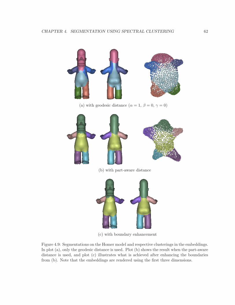
CHAPTER 4. SEGMENTATION USING SPECTRAL CLUSTERING 62
(a) with geodesic distance (α = 1, β = 0, γ = 0)
(b) with part-aware distance
(c) with boundary enhancement
Figure 4.9: Segmentations on the Homer model and respective clusterings in the embeddings.In plot (a), only the geodesic distance is used. Plot (b) shows the result when the part-awaredistance is used, and plot (c) illustrates what is achieved after enhancing the boundariesfrom (b). Note that the embeddings are rendered using the first three dimensions.

CHAPTER 4. SEGMENTATION USING SPECTRAL CLUSTERING 63
(a) colibri, 5 parts (b) hand, 6 parts (c) bixo, 11 parts
Figure 4.10: Segmentation results achieved with (bottom row) and without (top row) theVSI distance.
We demonstrate the effectiveness of the VSI distance component in Gc through more
tests and the results are presented in Figure 4.10. In this figure, parts in the bottom row
are achieved using the pre-set weights for the three distance components, while those in the
top row are obtained ignoring the VSI distance (α = 0.01, β = 0.99, γ = 0). It is clear that
when the VSI distance is in place, the parts obtained are of superior quality.
Finally, more segmentation results are given in Figure 4.11, which includes models with
genus greater than zero (vase, kitten, and dragon), as well as models with boundaries (heart).
Clearly, the segments obtained correspond to the constituent parts of the shapes that are
intuitive to human beings; the part boundaries have high quality as well.
Note that in all the above segmentation experiments, we set the dimensionality of face
embeddings equal to k; this is discussed in Section 4.3.1. k is the only user-input parameter
for this algorithm, and it is model-dependent. All other parameters are either fixed or

CHAPTER 4. SEGMENTATION USING SPECTRAL CLUSTERING 64
(a) heart, 5 parts (b) vase, 5 parts (c) kitten, 6 parts
(d) dragon, 7 parts (e) armadillo, 7 parts (f) dino-pet, 12 parts
Figure 4.11: Segmentations on a variety of different kinds of models.

CHAPTER 4. SEGMENTATION USING SPECTRAL CLUSTERING 65
automatically determined. Some heuristics [29, 59], including the eigen-gap [90], have been
proposed to automatically infer an appropriate k. We notice that such methods are not
sufficiently robust in general. Instead, we leave this problem to users.
Due to the super-quadratic complexity involved in the current algorithm, we have so far
only been able to deal with meshes with up to a few thousand faces. For this thesis, we test
our algorithms on a Windows machine with an AMD Opteron CPU at 2.41GHz and 8GB
RAM. Running the algorithm on the vase model (5000 faces) takes about 44 seconds. When
mesh size goes up, the computation time will increase rapidly and so will the space required
to store the affinity matrix W , which is not sparse. It would be intangible to handle a mesh
with hundreds of thousands of faces. We address this problem in the next chapter.
4.5 Summary
Our work in this chapter transforms the part information in the graph Gc to a face em-
bedding via a spectral embedding algorithm specifically designed for mesh segmentation.
Resorting to the analogy to KPCA, we justify our algorithm and address several issues im-
portant to the effectiveness of the face embedding. The final mesh segmentation result is
obtained from the embedding using the standard K-means clustering algorithm. In order to
improve its efficiency and quality, we propose methods to reduce the embedding dimension-
ality, initialize seed proxies, and enhance part boundaries. Experiments have shown that
our algorithm is able to extract parts from a shape with high quality.
However, the current algorithm is highly involved, incurring a complexity of O(n2 log n).
With such a super-quadratic complexity, the algorithm is only able to handle meshes with
up to several thousand faces. We address this issue in Chapter 5.

Chapter 5
Sub-sampling
5.1 Overview
The segmentation algorithm based on spectral clustering proposed in Chapter 4 has a high
computational cost — O(n2 log n). As it is normal to segment meshes with up to hundreds
of thousands of faces, we need to reduce its complexity for practical use.
We resort to sub-sampling for this purpose. Briefly, given an input mesh M with n
faces, we first compute a small set of sample faces Fs = fsi | 1 ≤ si ≤ n, i = 1, . . . , l,where l ∈ [2, n] is the sampling size. Then we construct only the corresponding rows of
the distance matrix G and the affinity matrix W . As the full W is unknown, we apply the
Nystrom method to approximate the eigenvectors of W . Afterwards, the construction of
the spectral embeddings of the faces and the K-means clustering are similarly conducted.
Meanwhile, we provide a geometric interpretation for the Nystrom method. This leads to
a practical quality measure for a sample set and a farthest-point sampling scheme we use
in practice. With sub-sampling, the overall complexity of the segmentation algorithm is
reduced to O(ml2) + O(l · n log n), where m = n− l.
In Section 5.2, we review the Nystrom method. Its geometrical interpretation is studied
in Section 5.3, through which a quality measure of sub-sampling is derived. With such a
quality measure, a farthest-point sampling scheme is suggested in Section 5.4. In Section 5.5
we modify the original segmentation algorithm to integrate sub-sampling. Experimental
results and summary are given in the last two sections.
66

CHAPTER 5. SUB-SAMPLING 67
5.2 Nystrom Method
The Nystrom method is one of the best known approximation schemes for sampling and
reconstruction for kernel techniques. It originates from finding numerical solutions of con-
tinuous eigenfunction problems [10] and has been applied by Williams and Seeger [132] for
providing low-rank approximation to kernel matrices and by Fowlkes et al. [38] for image
segmentation.
Consider a partition of a data set Z, |Z| = n, into two disjoint subsets X and Y, with
|X | = l, |Y| = m, respectively. Note that n = l + m and l ¿ m in practice. Without loss of
generality, we designate the points in X as samples and write the symmetric kernel matrix
K ∈ Rn×n for Z (recall that W can be considered as a kernel matrix) in block form:
K =
[A B
BT C
], (5.1)
where A ∈ Rl×l encodes the affinities between the points in X , C ∈ Rm×m encodes the
affinities between the points in Y, and B ∈ Rl×m encodes the inter-affinities between X and
Y. Let A = E∆ET be the eigenvalue decomposition of A, with the largest eigenvectors in
the leading columns of E, then the l leading eigenvectors of K can be approximated, using
the Nystrom method, by
E =
[E
BT E∆−1
], (5.2)
with columns of E containing the approximate eigenvectors. We see that only the sub-block
[A B] is required to compute E. The complexity involved is O(l3) + O(ml2), where the
first term is for computing the eigenvalue decomposition of A and the second term is for
computing BT E∆−1. Since l ¿ m, the complexity is essentially O(ml2).
With E, the reconstructed kernel matrix, K, can be computed as
K = E∆ET =
[A B
BT BT A−1B
]. (5.3)
The quality of the sample set X can then be quantified by ‖K − K‖F . Since K only
replaces block C of K with BT A−1B, this quantification is equivalent to ‖C −BT A−1B‖F ,
the Frobenius norm of the Schur complement (FNSC).

CHAPTER 5. SUB-SAMPLING 68
Note that the approximated eigenvectors in E are not normalized. Fowlkes et al. [38]
have shown how to meaningfully normalize them. However, we have found that such a
normalization works less preferably for our application.
The above discussion of the Nystrom method has assumed that the sampled rows are at
the leading rows of K for the sake of simplicity of presentation. In practice, we can simply
permute the sampled rows to the leading rows. Be aware that the respective columns have to
be consistently permuted as well to keep K symmetric. After the eigenvectors are computed,
their entries are permuted back accordingly to recover the original ordering. This process
is done implicitly and it is always assumed in the future that the leading rows of K are the
sampled rows.
5.3 Quality Measure
The Nystrom method only tells us how to extrapolate the eigenvectors given a subset of rows
of the kernel matrix K; it does not specify how to select the rows for better approximation
quality. FNSC is impractical for this purpose because C is unknown. In the following, we
provide a geometric interpretation for the Nystrom method and suggest a function Γ for
evaluating the quality of a sample set, which is much more efficient to evaluate.
Following the discussion in Section 4.2.2, we reiterate that K implicitly defines a mapping
φ(·) that maps set Z to φ(Z) = φ(zi)|zi ∈ Z in a high dimensional feature space H ∈Rh. Similarly, we have in the feature space φ(X ) for the sample set X and φ(Y) for its
complementary set. Suppose Xh×l = [φ(x1)|φ(x2)| . . . |φ(xl)] contains the mapped points
of φ(X ), and Y h×m and Zh×n are defined similarly. As the entries of K are the inner
products of φ(Z) in H, we have A = XT X, B = XT Y and C = Y T Y . It has been shown
in Section 5.2 that the Nystrom method approximates C with BT A−1B. We now examine
the geometric properties associated with this approximation.
Proposition 5.1. BT A−1B are the inner products between the points in φ(Y) after being
orthogonally projected into Space(φ(X )
), the space spanned by the points in φ(X ).
Proof. Denote by X+ the pseudo-inverse of X, i.e., X+ = (XT X)−1XT . Given any
point φ(yi) ∈ φ(Y), it is well known that φ(yi)’s orthogonal projection (also its clos-
est point) in Space(φ(X )
)can be computed as φ(yi)⊥ = (XX+)φ(yi). Having Y⊥ =
[φ(y1)⊥|φ(y2)⊥| . . . |φ(ym)⊥] = (XX+)Y , we obtain the pairwise inner products of the points

CHAPTER 5. SUB-SAMPLING 69
in φ(Y) after they are orthogonally projected into Space(φ(X )
)as
Y T⊥ Y⊥ = (XX+Y )T (XX+Y )
= Y T (X+)T XT X(X+Y )
= Y T((XT X)−1XT
)TXT X(X+Y )
= Y T XX+Y
= Y T X((XT X)−1XT
)Y
= (XT Y )T (XT X)−1(XT Y )
= BT A−1B
Therefore FNSC = ‖C − BT A−1B‖F = ‖Y T Y − Y T⊥ Y⊥‖F , and this implies that in
general the closer the points in φ(Y) are to Space(φ(X )
)the smaller FNSC is. When
Space(φ(Y)
) ⊆ Space(φ(X )
), we have Y = Y⊥ and BT A−1B = Y T
⊥ Y⊥ = Y T Y = C,
namely, BT A−1B reconstructing C exactly. With that said, the scale of FNSC can be
reflected by the overall distances from the points in φ(Y) to Space(φ(X )
). In fact, we have
Proposition 5.2. The trace of C −BT A−1B is the sum of the squared distances from the
points in φ(Y) to Space(φ(X )
).
Proof. Given a φ(yi) ∈ φ(Y), the squared distance from φ(yi) to Space(φ(X )
)is ‖φ(yi) −
φ(yi)⊥‖22 = ‖φ(yi)−XX+φ(yi)‖2. Then the sum of all the squared distances is
m∑
i=1
‖φ(yi)−XX+φ(yi)‖2 =m∑
i=1
(φ(yi)−XX+φ(yi)
)T (φ(yi)−XX+φ(yi)
)
=m∑
i=1
φ(yi)T (I −XX+)φ(yi)
=m∑
i=1
φ(yi)T φ(yi)−m∑
i=1
φ(yi)T (XX+)φ(yi)
= tr(C)− tr(Y T XX+Y )
= tr(C)− tr(BT A−1B
)
= tr(C −BT A−1B
)
where tr(·) is the matrix trace operator. The second last step is due to the fact Y T XX+Y =
BT A−1B, which is shown in the proof of Proposition 5.1.

CHAPTER 5. SUB-SAMPLING 70
−2 −1 0 1 2
−2
−1
0
1
2
y
x
(a) test point set
20 40 60 80 100 12020
40
60
80
100
120
140
160
FNSC
Γ
ρ = 0.9895
(b) (FNSC, Γ) observations
Figure 5.1: Strong correlation between FNSC and Γ. (a): The point set with a Gaussiandistribution, where the variances along x and y axes are 0.76 and 0.54, respectively. (b):Plot of the 100 observations to (FNSC, Γ). The correlation coefficient is ρ = 0.9895.
Via Proposition 5.1 and Proposition 5.2, we define function
Γ , tr(C)− tr(BT A−1B) (5.4)
to measure the quality of a sample set. We have shown that a small Γ would tend to lead
to a small FNSC. With Γ, we can evaluate the quality of a sample set without knowing
the entire C, which is needed when FNSC is used. Although C is not known, tr(C) can
usually be efficiently computed. In our implementation with equation 4.1, we have Wii ≡ 1,
in which case, tr(C) = m is a constant and only tr(BT A−1B) matters.
Figures 5.1 verifies the strong correlation between FNSC and Γ. In this experiment,
we generate 200 points with a Gaussian distribution, whose deviation along each axis is
randomly selected in (0, 1). The corresponding kernel matrix K is constructed using Eu-
clidean distance and an exponential kernel function. We randomly sample only 2 points and
the resulting pair (FNSC, Γ) is treated as an observation to their corresponding random
variables. We obtain 100 observations and the correlation of the two random variables is
0.9895. Clearly, FNSC and Γ are strongly correlated.

CHAPTER 5. SUB-SAMPLING 71
5.4 Sampling Scheme
Given a sampling size, our goal is to find the samples such that Γ is minimized. One
possible approach is to add samples iteratively, in a greedy manner: the next sample to
add is always the one that minimizes the current Γ. In short, the sampling scheme keeps
track of the current affinity matrices A and B. The next sample is selected as the one
such that the updated A and B would minimize Γ. Given the updated A and B, the
evaluation of Γ has a complexity of O(ml2). If carried out naively by evaluating Γ against
each data point, finding the next sample would cost O(m2l2), which is not acceptable. To
overcome this, we consider the best sampling scheme [120]. Instead of finding the next best
sample from all the remaining data points, we only try to find it among the best 1% with
probability 95%. Assuming that the columns of B are independent identically-distributed
(IID) random variables, we simply need to evaluate Γ on a random sample set of size
dlog(0.01)/log(0.95)e = 90, regardless of the data size. The overall complexity for finding
l samples with this approach would be O(90ln log n) + O(90ml3), where the first term is
for computing the geodesic distances from Gc to update A and B. We call this approach
Γ-sampling.
Although it achieves low asymptotic complexity, the Γ-sampling scheme is still not suf-
ficiently efficient due to the large constant in its complexity, especially for a dense mesh
(n is large). In practice, we use a more efficient farthest-point sampling scheme which is
suggested by an observation made on Γ.
In order to minimize Γ, we can aim to maximize tr(BT A−1B) as tr(C) is a constant in
our case. Based on the cyclic property of matrix trace, we have
tr(BT A−1B) = tr(A−1BBT ) = tr(A−1m∑
j=1
BjBTj ). (5.5)
With the assumption that the columns of B (Bj ’s) are random variables with IID distri-
bution, entries of∑m
j=1 BjBTj tend to be similar. We have observed such a property in
practice, especially when m is large. Therefore we can rewrite∑m
j=1 BjBTj ≈ κ11T , with
κ ∈ (0, m) being a fixed value, hence
tr(BT A−1B) ≈ κtr(A−111T ) = κ1T (A−11). (5.6)
From Equation 5.6, we see that there are two conditions for tr(BT A−1B) to attain a large
value: (1) a large 1T (A−11), and (2) a large κ.

CHAPTER 5. SUB-SAMPLING 72
Figure 5.2: The geometric examination of 1T (A−11) in R2. Suppose A = [1, α; α, 1], 0 ≤α ≤ 1, then the columns of A represent the coordinate basis shown as oa and ob. If we writeA−11 = [s; t], s and t can be computed geometrically by drawing lines pd and pc parallelto axes oa and ob, respectively. In other words, s = |oc|/|oa| and t = |od|/|ob|. It is easyto see s = |oc|/|oa| = |oe|/|ox| ≤ 1. Similarly, t = |od|/|ob| = |of |/|oy| ≤ 1. As a result,1T (A−11) = s + t ≤ 2. As oa and ob approach ox and oy, s + t keeps increasing until 2 isreached, at which time oa and ob turn into the canonical basis.
For condition (1), note that the vector A−11 contains the coefficients of the expansion
of 1 in the space whose basis are the columns of A, and the diagonals of A are 1 and the
off-diagonals are in the range [0, 1]. Figure 5.2 shows that, in 2D, 1T (A−11) ≤ l, where l
is the number of samples (l = 2 in this case). The equality is achieved when the columns
of A are the canonical basis. Since this can be generalized to arbitrary dimension and the
canonical basis mean that the off-diagonals of A are zeros, we should select samples such
that the affinities (distances) between them are as small (large) as possible.
Condition (2) requires κ to be large. To this end, entries of B should be large, indicating
that the distances between the sample faces and the un-sampled faces are small in average.
To satisfy condition (1), we have distributed sample faces mutually far apart on a mesh
surface. Therefore the average distances from the sample faces to the un-sampled faces tend
to converge, making condition (2) much less influential. Our experiments have also verified

CHAPTER 5. SUB-SAMPLING 73
that the first condition plays the dominant role.
In accordance with condition (1), we propose to sample faces that are mutually farthest
away using a max-min strategy as inspired by previous works, e.g., [34]. Given a distance
graph Gc, the sampling scheme works as in Figure 5.3. Note that step 1 attempts to find
the first two samples that are globally farthest apart efficiently. We do not find the exact
solution for this since it is expensive.
1. Randomly sample a face fsp and find the face fsq that is farthest to fsp . Switch fsp
and fsq and repeat this process until both faces stabilize. Then set fs1 = fsp ,fs2 = fsq , and Fs = fs1 , fs2.
2. Iteratively find the remaining samples. Specifically, select the next sample fsi as theone that maximizes the minimum distance to the previous samples fs1 , . . . , fsi−1 .
Figure 5.3: Farthest-point sampling scheme in max-min fashion.
Since the distances between faces are the graph distances in Gc, finding the face farthest
to a given one takes O(n log n) time. In step (2), whenever a new sample face is added,
we compute its distances to all the other faces. By maintaining the distances between
all the previous sample faces and the un-sampled faces, we can find the next sample face
in O(n) time. Since the convergence rate of step (1) is high (usually below 5 iterations),
the complexity is dominated by step (2), making the overall complexity of this sampling
algorithm O(l · n log n).
5.5 Modified Segmentation Algorithm
The modified segmentation algorithm based on spectral clustering with sub-sampling is
described in Figure 5.4. Overall it is similar to the case without sampling as described in
Section 4.2 and Section 4.3. However, it is worth mentioning the following issues.
• Given a sampling size l, the Nystrom method tells how to extrapolate l eigenvectors
approximately. However, it does not specify which original eigenvectors the extrap-
olated eigenvectors correspond to. Practically our experiments have shown that the
extrapolated eigenvectors correspond to the largest original eigenvectors. Roughly,
this can be understood by thinking of the eigenvectors as frequencies of the 2D signal

CHAPTER 5. SUB-SAMPLING 74
1. Compute sample face set Fs, |Fs| = l, as in Figure 5.3.
2. Calculate a partial distance matrix G′ that contains the rows (corresponding to thesamples) of the full distance matrix G. Convert G′ to a partial affinity matrix W ′,where W ′
ij = e−G′ij/2σ2
and σ is the square root of the average of the entries of G′.
3. Compute the l approximate eigenvectors for the affinity matrix W through W ′ withthe Nystrom method as in Section 5.2 (W is considered as the kernel matrix K).Denote by E the approximate eigenvectors and ∆ the eigenvalues of sub-block A.
4. Supposing all the eigenvalues of A are non-negative, derive the spectral embeddingU = E[2...l]∆
12 .
5. Treat the rows of U as the face embeddings, set the seed proxies as the embeddingsof the sample faces in Fs, and run the K-means algorithm.
Figure 5.4: Mesh segmentation based on spectral clustering with sub-sampling.
W [123, 124], where the largest eigenvectors correspond to low frequencies. When
sub-sampling, it is the low-frequency information that is reconstructed first. This
phenomenon is also observed by Belongie et al. [12].
• For the spectral embedding algorithm in Figure 4.2 without sampling, step (4) scales
the eigenvectors (V[2...r]) by the square root of the eigenvalues (Λ′12 ). With sub-
sampling, since the Nystrom method does not compute the eigenvalues of W , how
should we scale the approximate eigenvectors in E? It is noticed in [132] that the
eigenvalues of W are roughly nl times of those of A. Therefore we use the eigenvalues
of A to scale the approximate eigenvectors in E; the uniform scaling factor nl is ignored
without affecting the subsequent clustering.
• We have assumed that the eigenvalues of A are all positive. If not, we can simply
ignore the non-positive ones as described in 4.2.5. In fact, we have never encountered
such cases in our experiments. Since the eigenvalues of A and W are approximately
the same up to a scaling factor (nl ) and W always has positive leading eigenvalues
(Section 4.2.5), A’s eigenvalues are likely to be positive as well.
• In the clustering step, we could find the seed proxies as the embeddings that are
mutually farthest away (Section 4.3.2). But as the distances between the embeddings

CHAPTER 5. SUB-SAMPLING 75
mimic the distances in Gc (Section 4.2.6) and the faces in sample set Fs are computed
from Gc to be mutually farthest away, we can reuse this information by simply setting
the seed proxies as the embeddings of the sample faces. This makes the algorithm
more efficient.
Another issue we need to address is how to set l, the number of samples. As discussed
in Section 4.3.1, we set the dimensionality of the spectral embedding to k, the number
of segments given by a user. When sub-sampling, the number of samples determines the
number of eigenvectors in E. Therefore, we only need to set l = k + 1 in order to obtain
enough eigenvectors for embedding (note that the first approximate eigenvector is discarded
as it is close to a constant vector). Empirically, such a low sampling rate achieves high
segmentation quality while keeping the complexity low.
5.6 Experimental Results
Complexity Since our K-means algorithm has a high convergence rate, the asymptotic
complexity of the entire algorithm is dominated by the first three steps in Figure 5.4. Accord-
ing to the analysis in Section 5.2 and Section 5.4, the complexity of our spectral clustering
algorithm with sub-sampling is O(ml2) + O(l · n log n). In practice, we set l = k + 1.
Overview of experiments We have five experiments in this section. The first two
experiments test our sampling scheme with the Nystrom method in general. The last three
experiments demonstrate how the segmentation algorithm with sampling works on meshes.
In our first experiment, we test the performance of the farthest-point sampling method,
by measuring the difference between approximate eigenvectors and accurate eigenvectors.
For comparison purpose, we also test the Γ-sampling scheme described in Section 5.4. To
focus on the effect of sampling only, we consider points in R3, treating each point as a mesh
face and the Euclidean distances between points as the graph distances between faces in
Gc. We generate a total of 200 point sets and the reported result is the average of the
corresponding 200 tests. A point set is produced by a mixture of 10 Gaussian distributions.
Each Gaussian distribution has a random size between 30 and 60, with its mean at a random
point within a cube of side length 1 and deviations along each dimension randomly picked
from (0, 0.1]. Figure 5.5 shows the test results. In plots (a) and (b), we observe that the
approximation errors for both the second and the third eigenvectors decrease as the number

CHAPTER 5. SUB-SAMPLING 76
of samples increases. In fact, this is true for all other eigenvectors as well. Note that in
plot (b), the number of samples is at least 3; this is because the Nystrom method cannot
extrapolate more eigenvectors than the number of samples. Plot (c) shows the average
approximation error over all available eigenvectors given a sampling size. Since a larger
sampling size is able to extrapolate more trailing eigenvectors and the trailing eigenvectors
typically have lower approximation accuracy, we see that the average approximation error
for all eigenvectors increases when more samples are used. By this experiment, it is verified
that the farthest-point sampling consistently outperforms random sampling. Although it
does not perform as well as Γ-sampling, it is more efficient and works well in our experiments.
2 4 6 8 100.2
0.4
0.6
0.8
1
1.2
# of samples
appr
oxim
atio
n er
ror
random
farthest
Γ-
(a) for 2nd eigenvector
2 4 6 8 100.2
0.4
0.6
0.8
1
1.2
# of samples
appr
oxim
atio
n er
ror
random
farthest
Γ-
(b) for 3rd eigenvector
2 4 6 8 100.2
0.4
0.6
0.8
1
# of samples
appr
oxim
atio
n er
ror
random
farthest
Γ-
(c) for all eigenvectors
Figure 5.5: Approximation quality of eigenvectors via different sub-sampling methods. Theapproximation error is measured as the L2 norm of the difference between the original andthe approximate eigenvectors, up to sign flips.
The approximation quality of extrapolated eigenvectors through the Nystrom method
is also influenced by the tightness of clustering present in a point cloud. This phenomenon
is demonstrated in Figure 5.6. In this test, we build three point clouds in 2D shown in
the first column, and sample three points for each case. Each point cloud consists of three
Gaussian clusters centered at (0, 0), (10, 0), and (10, 10). Three levels of clustering tightness
are introduced by setting the deviations along x-axis and y-axis in each point cloud to 0.1,
1, and 3, respectively. The second (third) column shows, for the corresponding affinity
matrix W , the second (third) eigenvectors obtained with and without sub-sampling. It
is clear that if the clusters are tight and far apart from each other, the approximation
quality is high and vice versa. This is easy to explain according to Proposition 5.1 and
Proposition 5.2. For the ideal case in which the three clusters are infinitely far away and
the points within each cluster coincide with each other, based on the feature space distance

CHAPTER 5. SUB-SAMPLING 77
−4 0 4 8 12 16
−4
0
4
8
12
16
−0.2
−0.1
0
0.1
0.2
w/o samplingw/ sampling
−0.2
−0.1
0
0.1
0.2
w/o samplingw/ sampling
−4 0 4 8 12 16
−4
0
4
8
12
16
−0.2
−0.1
0
0.1
0.2
w/o samplingw/ sampling
−0.2
−0.1
0
0.1
0.2
w/o samplingw/ sampling
−5 0 5 10 15 20
−5
0
5
10
15
20
−0.2
−0.1
0
0.1
0.2
w/o samplingw/ sampling
−0.2
−0.1
0
0.1
0.2
w/o samplingw/ sampling
Figure 5.6: Quality of approximate eigenvectors is influenced by the tightness of clustering.In each row, the first plot shows a point cloud with a certain degree of clustering tightness,where the red circles indicate the three sample points chosen by our farthest-point sam-pling. The second plot and the third plot illustrate the second and the third eigenvectors,respectively, of the affinity matrix W derived from the corresponding point cloud, with andwithout sub-sampling.

CHAPTER 5. SUB-SAMPLING 78
calculation (Equation 4.16), each cluster degenerates to a single point in the feature spaceH.
Therefore the three sample points span the entire space spanned by all the points in H; in
other words, we have Space(φ(X )
)= Space
(φ(Y)
). This implies Γ = 0 and the eigenvector
extrapolation is exact. On the other hand, if the clusters are loose and overlap with each
other, points will be scattered out in H. Then Space(φ(X )
)would tend to occupy only a
small subspace of Space(φ(Y)
), causing large Γ and lower approximation quality in general.
With this being said, a sensitive part-aware metric, as the one described in Chapter 3, not
only contributes to a face embedding easy for the K-means algorithm to extract prominent
clusters, but also helps the sub-sampling method achieve high accuracy.
Let us now apply the spectral clustering algorithm with sub-sampling to two small
meshes used in Section 4.4, and compare the approximate eigenvectors with the accurate
ones. In Figure 5.7, the two columns show the segmentation results, the original, and the
approximated eigenvectors of the enforcer model and the armadillo model, respectively.
Compared with those in Figure 4.7(a) and Figure 4.11(e), almost the same segmentation
results are achieved with sub-sampling. For each model, we also see that the extrapolated
eigenvectors (blue) approximate the accurate ones (red) reasonably well, which is why the
segmentation quality under sub-sampling is not significantly sacrificed. Reminiscent of the
analysis for Figure 5.6, the approximation quality of eigenvectors for the enforcer model is
higher than that for the armadillo model, since the faces of the enforcer form tighter clusters
due to the larger distance changes across the part boundaries. It is worth reiterating that
we only set the sample number to k + 1 (k is the number of segments) as mentioned in
Section 5.5; if we increase the sampling rate, better approximation quality is expected. In
practice, we found that such a low sampling rate is sufficient.
Recall the comparison of the distance fields shown in Figure 3.9. Since the three meshes
are too large, we were unable to handle them in Chapter 4 before the sub-sampling is
introduced. In Figure 5.8, segmentation results on these three meshes via sub-sampling are
shown. Again, to demonstrate the effectiveness of VSI distance, we also give in the top
row the segmentation results obtained using only geodesic and angular distances (α = 0.01,
β = 0.99, and γ = 0). For example, the fingers of the hand model are better segmented
off the palm along the intuitive boundaries in the bottom row. So are the horse’s front leg
and right ear, and the dragon’s left arm and tail. These are the natural consequences of the
sudden distance changes across those regions as shown in the bottom row of Figure 3.9.
Finally, more segmentations on a variety of models are reported in Figure 5.9. Note that

CHAPTER 5. SUB-SAMPLING 79
enforcer, 5 parts armadillo, 7 parts
−0.04
−0.02
0
0.02
0.04
w/o samplingw/ sampling
2nd eigenvectors
−0.1
−0.05
0
0.05
0.1
w/o samplingw/ sampling
2nd eigenvectors
−0.04
−0.02
0
0.02
0.04
w/o samplingw/ sampling
3rd eigenvectors
−0.2
−0.1
0
0.1
0.2
w/o samplingw/ sampling
3rd eigenvectors
Figure 5.7: Segmentations of two models via sub-sampling and the eigenvectors. In eachcolumn, both the second and the third eigenvectors obtained with (blue) and without (red)sampling are drawn.

CHAPTER 5. SUB-SAMPLING 80
(a) hand, 7 parts (b) horse, 9 parts (c) dragon, 9 parts
Figure 5.8: Segmentation results achieved with (bottom row) and without (top row ) VSIdistance.

CHAPTER 5. SUB-SAMPLING 81
(a) bone, 3 parts (b) snake, 4 parts (c) teapot, 4 parts
(d) dilo, 7 parts (e) camel, 7 parts (f) cat, 9 parts
Figure 5.9: Segmentation results of various models with sub-sampling.
both the teapot and the camel have genus greater than 0. High quality segmentation results
are achieved on all these models using a small number of samples. For the dilo model with
about 55K faces, our algorithm takes only about 4 seconds. If we subdivide the model into
220K faces, only 13 seconds are needed.
5.7 Summary
We integrate sub-sampling to the mesh segmentation algorithm described in Chapter 4.
The complexity of the new algorithm is significantly reduced from O(n2 log n) to O(ml2) +
O(l · n log n), where l is the number of samples and m = n − l. In our application, we set
l = k + 1 ¿ n, with k being the desired number of segments given by users. With such a
low sampling rate, the size of meshes that our algorithm can handle increases from several

CHAPTER 5. SUB-SAMPLING 82
thousands to hundreds of thousands.
Our sub-sampling scheme is based on the Nystrom method, a popular technique for
computing approximate eigenvectors of a symmetric matrix when only a subset of its rows
are available. By examining the geometric meaning of the Nystrom method, we propose a
function Γ to evaluate the sampling quality. Eventually, a farthest-point sampling scheme
is used to optimize for Γ approximately. The experiments have demonstrated that our sub-
sampling approach is able to achieve comparable segmentation results with higher efficiency.
We also notice two limitations of the current segmentation algorithms, with and with-
out sub-sampling. First, it requires users to input the number of segments k. Segmentation
quality could suffer if k is not set appropriately. Secondly, although the part-aware distance
enhances the clusters in the embedding space, prominent parts may still be missed occasion-
ally due to the limitations of the K-means clustering, especially when the desired k is large,
such as for those shown in Figure 6.18(f) and Figure 6.19(f). The algorithm proposed in
Chapter 6 improves on these issues by incorporating segmentability and salience, but with
higher computational cost.

Chapter 6
Segmentation Driven by
Segmentability and Salience
6.1 Overview
In this chapter, we improve upon the previous segmentation algorithm by introducing seg-
mentability and salience-driven cut. Rather than using a simultaneous k-way partitioning,
the improved algorithm iteratively bisects mesh parts. In each iteration, a mesh part with
the largest surface area is considered. If the mesh part has a segmentability score above a
fixed threshold, it is cut into two sub-parts, which are to be considered for further segmen-
tation; otherwise this mesh part is deemed not segmentable and becomes an output part. In
order to find the best cut, the faces of the selected mesh part are first sorted into a sequence.
Then the algorithm searches through this sequence, measures the salience at each location,
and chooses the cut that has the highest salience score. Figure 6.1 illustrates the flow of
this algorithm. Such an algorithm has the following merits:
• Segmentability provides a robust quantitative evaluation as to whether a shape con-
tains any parts. Accordingly, our algorithm can fix a segmentability threshold as the
stopping criteria for the iterative cut. Note that a single segmentability threshold
works for different models, while the number of segments used in the previous algo-
rithm is model-dependent. Thus, the improved algorithm achieves higher autonomy.
• With mesh faces sorted in a sequence, the search space for the best cut is significantly
reduced. This makes the salience-driven cut search affordable. Computed carefully,
83

CHAPTER 6. SEGMENTATION DRIVEN BY SEGMENTABILITY AND SALIENCE 84
input : Mesh M.output: Sub-meshes O = M1,M2, ....begin
O = ∅, Q = M ;η = 0.1 ;while |Q| 6= 0 do
Mc ← the mesh piece in Q with the largest surface area ;Q = Q− Mc ;S ← Segmentability(Mc) ; /* Section 6.2 */if S ≥ η then
% = FaceLinearization(Mc) ; /* Section 6.3 */
M′s,M′
s ← SalienceCut(Mc, %) ; /* Section 6.4 */
Q = Q⋃M′s,M′
s ;else
O = O⋃Mc ;end
endend
Figure 6.1: Mesh segmentation driven by segmentability and salience.
the sequence also effectively preserves the meaningful cuts.
• By incorporating a salience measure mimicking human intuition for parts into the cut
search, the segmentation quality is enhanced.
In Section 6.2, we discuss the concept of segmentability within our context and show
how the segmentability analysis is performed. Once a mesh part passes the segmentability
test, Section 6.3 studies how to obtain an effective face sequence for the subsequent salience-
driven cut search, which is discussed in Section 6.4. Experiments are given in Section 6.5
and Section 6.6 presents the summary.
6.2 Shape Segmentability
Instead of letting users provide the number of segments for each input mesh, it is desirable
to have an algorithm that can figure out this information on its own. To fulfill this goal, we
want to tell when a mesh has any parts, or, in other words, is segmentable. A key observation
we make is that there are two primary factors that can render a shape segmentable. The

CHAPTER 6. SEGMENTATION DRIVEN BY SEGMENTABILITY AND SALIENCE 85
first one is the branching factor. That is, if a shape has branches, then it is segmentable.
We refer to the segmentability caused by branching as structure segmentability. The second
factor is due to concavity over the boundary of a part in the absence of branching, where
the induced segmentability is referred to as geometry segmentability. Do not confuse these
two terms with structural-level and geometrical-level segmentations. In our context, both
structure and geometry segmentabilities are for the structural-level segmentation.
Obtaining either the structure or the geometry segmentability information from a 3D
mesh is rather difficult and inefficient. As a solution, we project the mesh into 2D and ex-
ploit the outer contour of the 2D projection for segmentability analysis. It is not a surprise
that a significant amount of information may be lost when going from 3D to 2D. However, by
carefully manipulating the projecting procedure, we are able to preserve, and even enhance,
the part information useful for the subsequent shape analysis. In our approach, structure
and geometry segmentability information are extracted from 3D meshes separately, using
two projection operators: L and M . Note that the resulting projections are essentially 2D
spectral embeddings. In order to differentiate this operation from the spectral embedding
for K-means (Section 4.3), we call these 2D embeddings for segmentability analysis seg-
mentability projections, or simply projections. For simplicity, we refer to a projection via L
(M) as L-projection (M -projection). We study both projection operators as follows.
6.2.1 Structure Projection
Given an input mesh with n vertices, its graph Laplacian L ∈ Rn×n is defined as L = D−T ,
where Tij = 1 whenever (i, j) is an edge, otherwise Tij = 0; D is a diagonal matrix whose
diagonals are row sums of T . Hence the affinity Tij between vertices is determined only
by their connectivity. Let L = ΞΛΞT be the eigenvalue decomposition of L, where the
eigenvalues in Λ are in ascending order. It is well known that L is positive semidefinite
with the smallest eigenvalue λ1 = 0 and the corresponding eigenvector Ξ1 being a constant
vector. Since L is symmetric, its eigenvectors are orthogonal and span the entire space
Rn×n.
Suppose the rows of X ∈ Rn×3 contain the coordinates of the vertices of the input
mesh. Then X can be written as a linear combination of the eigenvectors of L (since the
eigenvectors span the entire space). Projecting X into the subspace spanned by the first k
eigenvectors of L, we obtain
X = Ξ[1...k]ΞT[1...k]X,

CHAPTER 6. SEGMENTATION DRIVEN BY SEGMENTABILITY AND SALIENCE 86
(a) a foot mesh (b) L-projection
Figure 6.2: L-projection (b) of a foot model (a) with branching structure. Color dotsindicate correspondence.
where Ξ[1...k] denotes the first k columns of Ξ. This projection process can also be seen as
applying an ideal low-pass filter (only allowing the leading k frequencies to “pass”) to the
mesh coordinate signal, akin to Laplacian smoothing [123]. Choosing k = 3, we obtain a
planar shape, since the first eigenvector is a constant vector.
As a result of Laplacian smoothing, high-frequency information, e.g., surface fluctua-
tions, in the original shape is removed, while low-frequency (high-level) shape characteristics,
e.g., branching, is retained and even enhanced in the 2D projection. Figure 6.2 illustrates
this property. The five toes of the foot mesh, shown in plot (a), form branches. Plot (b)
shows its 2D L-projection. As observed, the “toe branches”, as a low-frequency structure,
is extracted and enhanced in the 2D projection space.
6.2.2 Geometry Projection
Although projecting using the L operator is able to reveal the structure segmentability of
a shape, it may fail to capture geometry segmentability information since L is only defined
by mesh connectivity. Figure 6.3 depicts such a situation. We see that the original mesh
(a) is clearly segmentable due to the concavity between the handle part and the body
part. However, since there is no branching structure in place, its L-projection (b) does not
exemplify strong segmentability; this could introduce difficulty to the subsequent analysis.
To resolve this issue, we design a new Laplacian operator M . M is defined similar to L
as M = D − T , with the only exception that the entries of T herein need to take into

CHAPTER 6. SEGMENTATION DRIVEN BY SEGMENTABILITY AND SALIENCE 87
(a) a cheese mesh (b) L-projection (c) M -projection
Figure 6.3: Segmentability of a cheese model is better revealed in the M -projection.
consideration the geometric information of a mesh surface. To this end, we define for edge
e = (i, j) its corresponding entry Tij as
Tij =
(|κi|+ |κj |) · |〈e, z〉| · l if κi < 0 or κj < 0,
ε otherwise.
κi and κj , computed as in [26], are the minimal principal curvatures at vertices vi and
vj , z is the normalized average of the principal curvature directions of κi and κj , e is the
normalized direction of e, and l is the length of e divided by the average length of all edges
in this mesh. When κi ≥ 0 and κj ≥ 0, implying local convexity at e, we set Tij = ε = 0.1
to simply maintain vertex connectivity information in T . If (i, j) is not an edge, Tij = 0.
We see that if an edge is roughly aligned up with the local minimal curvature direction and
any of the end vertices of this edge has negative minimal curvature, this edge would carry a
large weight. We examine the effect of this weighting scheme on the projection as follows.
Consider any matrix Y ∈ Rn×k, it can be shown that
12
∑
ij
Tij ||yi − yj ||2 = tr(Y T (D − T )Y
)= tr(Y T MY ), (6.1)
where Y = [yT1 |yT
2 | . . . |yTn ]T and each yi, a row vector, is seen as a k-dimensional point. Let
M = ΞΛΞT be the eigenvalue decomposition. The first (smallest) k eigenvectors of Ξ can
be denoted, in column and row vector format, by Ξ[1...k] = [ξ1|ξ2| . . . |ξk] = [uT1 |uT
2 | . . . |uTn ]T .
It is known that when Y = Ξ[1...k], i.e., yi = ui, i = 1 . . . k, Equation 6.1 is minimized,
under the constraint that the columns of Y are of unit length. With a large weight Tij ,

CHAPTER 6. SEGMENTATION DRIVEN BY SEGMENTABILITY AND SALIENCE 88
Equation 6.1 should be minimized with small ||yi−yj ||2. Since ui and uj are the minimizers,
it induces that ||ui − uj ||2 should be small, given a large Tij .
Similar to Section 6.2.1, we obtain the projection X = Ξ[1...k]ΞT[1...k]X. It follows that
the squared distance between two embedded vertices, xi and xj (two rows of X), is
||xi − xj ||2 = ||(ui − uj)ΞT[1...k]X||2 ≤ ||ui − uj ||2||ΞT
[1...k]X||2.
Given a large Tij , ||ui−uj ||2 is relatively small as reasoned above; therefore ||xi−xj ||2 should
also be relatively small, since ||ΞT[1...k]X||2 is a constant. Thus for each pair of vertices, a
larger Tij suggests that their embeddings should be closer to each other. With the way the
weights in T are defined, mesh vertices from a concave region are to be pulled closer to
each other after the projection, helping form a constriction in the projection space between
the two parts. This is illustrated in Figure 6.3(c), where we see that the concavity between
the handle part and the body part of the cheese mesh leads to an aggressively constricted
region in the M -projection, thus a greatly enhanced segmentability. It is worth pointing
out that the concavities from the circular dents in the body part do not contribute to any
segmentability, as they are “contained” within the shape and do not influence the resulting
outer contour of the M -projection. Therefore, only the handle part, but not the dents, is
to be segmented off the body part and this is intuitive (see Figure 6.19(b)).
6.2.3 Contour Extraction and Pre-processing
Our segmentability analysis is based on the outer contour of a 2D L-projection or a M -
projection. Therefore we need to extract the contour of a projection first. This is done by
rendering in black the faces of the projected mesh against a white background and tracing
the outer boundary of the resulting binary image. In our application, we set the image
resolution to 200 × 200. As the mesh is connected, so is the rendered region. Ignoring
interior holes, which can be caused by the openings of the mesh piece, we obtain a single
continuous outer contour of the 2D projection. Since the traced contour consists of discrete
pixels and is usually jaggy, we smooth it first using truncated Fourier descriptors (FDs)[142].
Intuitively, low-frequency FDs correspond to the smooth and approximate shape of the con-
tour, while high-frequency FDs correspond to local noise on the contour. In our smoothing,
low-frequency FDs are added one by one until the reconstruction error (measured by the
overall distance between corresponding points from the reconstructed contour and the orig-
inal contour) falls below a threshold, which is set to be 0.5% of the scale of the contour.
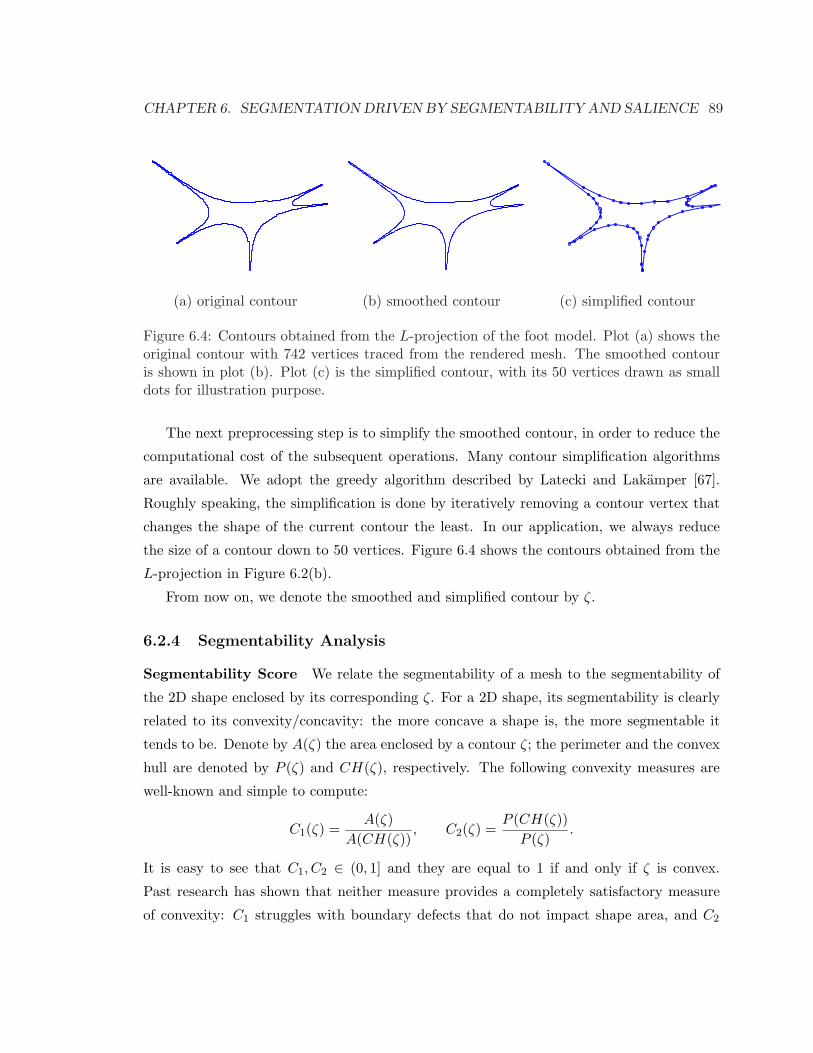
CHAPTER 6. SEGMENTATION DRIVEN BY SEGMENTABILITY AND SALIENCE 89
(a) original contour (b) smoothed contour (c) simplified contour
Figure 6.4: Contours obtained from the L-projection of the foot model. Plot (a) shows theoriginal contour with 742 vertices traced from the rendered mesh. The smoothed contouris shown in plot (b). Plot (c) is the simplified contour, with its 50 vertices drawn as smalldots for illustration purpose.
The next preprocessing step is to simplify the smoothed contour, in order to reduce the
computational cost of the subsequent operations. Many contour simplification algorithms
are available. We adopt the greedy algorithm described by Latecki and Lakamper [67].
Roughly speaking, the simplification is done by iteratively removing a contour vertex that
changes the shape of the current contour the least. In our application, we always reduce
the size of a contour down to 50 vertices. Figure 6.4 shows the contours obtained from the
L-projection in Figure 6.2(b).
From now on, we denote the smoothed and simplified contour by ζ.
6.2.4 Segmentability Analysis
Segmentability Score We relate the segmentability of a mesh to the segmentability of
the 2D shape enclosed by its corresponding ζ. For a 2D shape, its segmentability is clearly
related to its convexity/concavity: the more concave a shape is, the more segmentable it
tends to be. Denote by A(ζ) the area enclosed by a contour ζ; the perimeter and the convex
hull are denoted by P (ζ) and CH(ζ), respectively. The following convexity measures are
well-known and simple to compute:
C1(ζ) =A(ζ)
A(CH(ζ)), C2(ζ) =
P (CH(ζ))P (ζ)
.
It is easy to see that C1, C2 ∈ (0, 1] and they are equal to 1 if and only if ζ is convex.
Past research has shown that neither measure provides a completely satisfactory measure
of convexity: C1 struggles with boundary defects that do not impact shape area, and C2

CHAPTER 6. SEGMENTATION DRIVEN BY SEGMENTABILITY AND SALIENCE 90
is sensitive to noise. However, they appear to complement each other [149]. Motivated by
this, we propose to use the following simple extension as our convexity measure,
C(ζ) = maxC1(ζ), C2(ζ)wcvx,
where the exponent wcvx ≥ 1 not only ensures that C ∈ (0, 1] and C = 1 if and only if ζ
is convex, but also addresses possible differences in scale between C1 and C2. Throughout
our experiments, we set wcvx = 4.
C1 = 0.3878
C2 = 0.9823
C =0.9311
C1 = 0.7987
C2 = 0.8242
C = 0.7987
C1 = 0.3858
C2 = 0.7962
C = 0.4019
Figure 6.5: Convexity measures of three shapes based on area and perimeter.
For a telling example which illustrates the advantage of our convexity measure, consider
the rough outlines of the letters I and R, shown in Figure 6.5. By C1, I is deemed to be
more concave and thus more segmentable than R; this is counter-intuitive. With the new
measure C, Cwcvx2 would prevail over C1 for I and return a more reasonable result. The new
measure can also properly rank the convexity between the outlines of the letters I and C.
The potentially large discrepancies between C1 and C2, e.g., for I, explains our preference
of using the max operator over a convex combination. The inability of either C1 or C2 to
properly capture the convexity of a shape should not diminish the utility of the other.
Finally, with the convexity measure in place, we define the segmentability score, S(ζ),
of a contour ζ as
S(ζ) = 1− C(ζ). (6.2)
Clearly, S(ζ) ∈ [0, 1) and the larger S(ζ) is, the more segmentable ζ is.
Articulation Invariance Despite a correlation between convexity and segmentability,
they are not exactly the same concept. Naturally, the result of structural-level segmentation
should be invariant to shape articulation and this should also hold for a segmentability mea-
sure. However, the same cannot be said about convexity/concavity. The effect of bending

CHAPTER 6. SEGMENTATION DRIVEN BY SEGMENTABILITY AND SALIENCE 91
(a) C = 0.9557. (b) C = 0.9084.
(c) C = 0.7809. (d) C = 0.6275.
Figure 6.6: Use of MDS to enhance the performance of segmentability measure. The shapesin (a) and (b) compromise the effectiveness of C. However, they can be “stretched out” viaMDS using inner distances, as shown in (c) and (d), respectively, for more intuitive results.
can compromise the performance of the convexity measure C, and hence the segmentability
measure S. The contours illustrated in Figure 6.6(a, b) give two such examples: though
the two contours are sufficiently segmentable (due to the deep concavity), their convexity
measures are in fact close to 1 (segmentability close to 0).
Our solution to this problem involves normalizing contours with respect to shape ar-
ticulation, using Multi-Dimensional Scaling (MDS) [27]. Roughly speaking, given pairwise
distances between a set of points, MDS embeds the points in Euclidean space, while pre-
serving the original distances through the new Euclidean distances as much as possible.
If there is a distance measure between contour vertices that is insensitive to bending, we
can use MDS based on this distance measure to re-embed the contour vertices, and the
resulting contours are therefore invariant to articulation. We resort to inner distances [77]
to achieve this goal. The inner distance between two vertices u and v on a contour ζ is
defined as the length of the shortest path between u and v which lies in the interior of ζ.

CHAPTER 6. SEGMENTATION DRIVEN BY SEGMENTABILITY AND SALIENCE 92
As shown in Figure 6.6 (a) and (b), the red dotted lines depict the shortest paths between
the corresponding contour vertices inside the shape. Ling and Jacob [77] first propose the
use of inner distances for the retrieval of articulated shapes and they have shown that inner
distances are insensitive to shape articulation.
A natural way to compute pairwise inner distances between n contour vertices is to
first construct a visibility graph, where the nodes are the contour vertices and each pair
of nodes are connected by an edge if and only if the line segment between them are inside
the contour. After the visibility graph is constructed, the inner distance between any two
contour vertices is simply their shortest graph distance in the visibility graph. A simple
implementation of this method has a complexity of O(n3), due to the construction of the
visibility graph. Theoretically speaking, there is an optimal O(n) scheme for finding inner
distances emanating from a vertex, leading to an overall complexity of O(n2). However,
this scheme relies on the linear-time polygon triangulation algorithm of Chazelle [22], which
is generally believed to be extremely hard to implement. We have opted to implement the
simplistic O(n3) approach since each contour ζ we need to analyze has only 50 vertices after
the contour simplification.
After the pairwise inner distances are computed, we perform MDS to embed the contour
onto a plane. The inner distances are approximated by Euclidean distances via MDS and as
such, the contour is normalized against bending. Two results of MDS via inner distances are
shown in Figure 6.6(c, d). The convexity measure C can then be applied to the normalized
contours, successfully recognizing the two shapes with high segmentability scores.
Segmentability Analysis Procedure As illustrated in Figure 6.1, supposing the mesh
pieces that have not been classified as output parts are stored in the set Q, our algorithm
always selects from Q the mesh piece Mc with the largest surface area for the current
segmentation. Figure 6.7 recapitulates the segmentability analysis on Mc, where returned
value TRUE indicates Mc is segmentable and vice versa. η (= 0.1) is the segmentability
threshold value.
To consider both structure and geometry segmentabilities, we conduct contour analysis
on ζL and ζM in order. For each contour, we also examine its normalized counterpart, ζ∗Lor ζ∗M , via MDS to achieve articulation invariance. If all the four thresholding tests fail
(FALSE returned), Mc is deemed not segmentable and becomes an output part; otherwise
Mc is to be segmented by our salience-driven cut algorithm, which we discuss next.

CHAPTER 6. SEGMENTATION DRIVEN BY SEGMENTABILITY AND SALIENCE 93
1. Compute ζL, the contour of the L-projection of Mc. If S(ζL) > η, return TRUE.
2. Compute the MDS-embedding ζ∗L of ζL via inner distances. If S(ζ∗L) > η, returnTRUE.
3. Compute ζM , the contour of the M -projection of Mc. If S(ζM ) > η, return TRUE.
4. Compute the MDS-embedding ζ∗M of ζM via inner distances. If S(ζ∗M ) > η, returnTRUE.
5. return FALSE.
Figure 6.7: Contour segmentability analysis procedure.
6.3 Face Linearization
Once the current mesh piece Mc is deemed segmentable, it is subject to the actual segmen-
tation. The segmentation procedure has two steps: arrange the faces of Mc in a sequence,
and search through the sequence to obtain the most salient cut. We call the first step face
linearization and discuss it in this section. The second step is discussed in Section 6.4.
Recall that we have defined the part-aware graph Gc in Section 3.5 and the induced
graph distances have been used for the segmentation algorithm in Chapter 4. Supposing Gc
is the corresponding part-aware graph of Mc, we want to use Gc again to derive the face
sequence for Mc. However, we cannot construct Gc for Mc in the same way any more. This
is because the current algorithm segments iteratively and the intermediate mesh piece Mc
is open. Since an open mesh in general does not admit a well-defined enclosed volume, the
VSI-distance component in Gc is no longer robust. Therefore we only consider the geodesic
and angular distances and build the corresponding graph G′c similarly. Although G′
c is no
longer equipped with VSI-distance, the face linearization and salience-driven cut are still
able to ensure high quality segmentation results.
In order to linearize the faces effectively so that the meaningful cuts are preserved in
the resulting sequence, we first need to find two sample faces which are from two different
parts of Mc. We discuss this issue in Section 6.3.3. Assuming we have already obtained G′c
and the two sample faces fs and ft, the computation of the sequence per se turns out to be
fairly simple. Let’s denote by dis and dit the graph distances in G′c between fi and fs, fi

CHAPTER 6. SEGMENTATION DRIVEN BY SEGMENTABILITY AND SALIENCE 94
and ft, respectively. We then define a vector e, where e(i) = dis − dit. By sorting e,
[es, %] = sort(e), (6.3)
we have es as the sorted vector, say in ascending order, and % as the index vector of es. For
example, if e(a) ≤ e(b), a would proceed b in %. % is the face sequence we seek.
Although simple, the sequence % has a variety of nice features that make it suitable to be
used for our salience-driven cut search. We discuss this sequence in detail in the following.
6.3.1 Derivation and Properties
In Chapter 5, we have adopted sub-sampling and the Nystrom method to compute the
approximate eigenvectors of W to reduce complexity. If we sample only two faces, the sub-
block A in Equation 5.1 reduces to [1 α; α 1], with 0 ≤ α ≤ 1 being the affinity between
sample faces fs and ft. The sub-block B can be written as
B =
[. . . xi . . .
. . . yi . . .
], (6.4)
where xi (yi) is the affinity between fi and fs (ft). For the simplicity of notation, we assume
that the faces are re-indexed so that fs and ft are the first two faces and fi, 3 ≤ i ≤ n, is
an un-sampled face. Note that this does not affect the properties of %.
Following the formula in Equation 5.2, it is not hard to show that the two approximated
eigenvectors using only two samples are
E =12
1 −1
1 1
. . . . . .yi+xi1+α
yi−xi1−α
. . . . . .
. (6.5)
So the component-wise ratio of the second eigenvector (E·2) to the first eigenvector (E·1) is
e =[−1, 1, . . . ,
(yi − xi
yi + xi· 1 + α
1− α
), . . .
]. (6.6)
If we consider e as a 1D embedding of the mesh faces, we have e(fs) = −1, e(ft) = 1, and
e(fi) = yi−xi
yi+xi· 1+α
1−α . Let’s write the affinities between the faces based on their distances as
α = e−dst/2σ2, xi = e−dis/2σ2
, and yi = e−dit/2σ2, where dis and dit are mentioned above,
and dst is the graph distance between sample faces fs and ft. We prove two properties of e.

CHAPTER 6. SEGMENTATION DRIVEN BY SEGMENTABILITY AND SALIENCE 95
Proposition 6.1. ∀fi, e(fs) ≤ e(fi) ≤ e(ft). This means that the embeddings of the two
sample faces fs and ft are at the two ends of e.
Proof. We only prove e(fi) ≤ e(ft). e(fs) ≤ e(fi) can be proved similarly.
e(fi) ≤ e(ft) ⇔ yi − xi
yi + xi· 1 + α
1− α≤ 1
⇔ (yi − xi)(1 + α) ≤ (yi + xi)(1− α)
⇔ αyi − xi ≤ −αyi + xi
⇔ α ≤ xi
yi
⇔ e−dst/2σ2 ≤ e(dit−dis)/2σ2
⇔ −dst ≤ dit − dis
⇔ dis ≤ dit + dst.
Since the graph distance in G′c is a metric, satisfying the triangle inequality, the last in-
equality holds. This concludes our proof.
Proposition 6.2. Sorting vectors e or e produces the same face sequence.
Proof. For e, let’s denote F (fi) = yi−xiyi+xi
· 1+α1−α . Representing β = xi/yi, we can also write
F (β) = 1+α1−α · (1− 2
1/β+1). Clearly F (β) is monotone and inversely proportional to β. Mean-
while, as β = e−dis/2σ2/e−dit/2σ2
= e−(dis−dit)/2σ2, β is monotone and inversely proportional
to (dis − dit). Therefore F is monotone and proportional to (dis − dit). This implies that
except for the two sample faces, the face sequences obtained by sorting e and e are identical.
Due to the triangle inequality, it is easy to see that (dis − dit) is minimized when i = s and
maximized when i = t. As a result, the two sample faces are sitting at the two ends of e.
Plus Proposition 6.1, we prove that the two sequences are the same. Note that we have
assumed that neither e nor e has equal entries. If they do, we can mandate that the sorting
algorithm be stable to ensure the same sequence.
With Proposition 6.1 and Proposition 6.2, we have:
• fs and ft are always at the two ends of sequence %, and
• the sequence % from Equation 6.3 is the same with the sequence obtained by sorting
e from Equation 6.6.

CHAPTER 6. SEGMENTATION DRIVEN BY SEGMENTABILITY AND SALIENCE 96
(a) (b)
Figure 6.8: Characteristics of a face sequence produced for a synthetic 2D shape. Plot (a)shows the shortest paths between faces fi, fj and the sample faces fs and ft, where thearrow at the bottom indicates the rough direction of the corresponding face sequence. Inplot (b), the sequence is shown with gray-scale colors: each jump in the sequence causesan equal shift in the color space. The meaningful cut is available in such a sequence, asindicated by the vertical dashed line.
First, this implies that we must select two sample faces from two different parts; otherwise,
counter-intuitive results would be produced, since any cut sought from % would have to
separate the samples which are at the two ends of % into different parts. Secondly, as e is
spectral-based, % can be considered spectral-based as well.
As a concrete example, Figure 6.8 illustrates how the faces from a synthetic 2D shape
are arranged in %, given a sample pair. In this toy example, the distance we use is the inner
distance (Section 6.2.4). For faces fi and fj as configured in plot (a), it is apparent that
djs − djt < dis − dit; therefore fj is closer to fs in % than fi is to fs. The face sequence
roughly follows the order: fs → . . . → fj → . . . → fi → . . . → ft. Plot (b) color-codes the
corresponding sequence, where brighter colors indicate positions closer to fs. The migration
of the brightness attests to our analysis.
There is no doubt that arranging faces in % could potentially eliminate some meaningful
cuts. However, the cut producing the two parts from which the sample faces were selected are
most likely to be well preserved. Figure 6.9 gives an intuitive explanation. In plot (a), let’s
first presume that the two sample faces fs and ft are from the tips of the second and the third
fingers, which is what our sampling approach (Section 6.3.3) tends to do. We also assume
that the joint region between the second finger and the palm contains a single face fi. Based
on the previous analysis, we know that fs is at one end of % and, clearly, the faces between fs
and fi on the surface sit between fs and fi in %. We have shown that the position of fi in % is

CHAPTER 6. SEGMENTATION DRIVEN BY SEGMENTABILITY AND SALIENCE 97
(a) (b)
(c) (d)
Figure 6.9: The effectiveness of the face sequence in preserving desirable cuts. (a): theshortest paths between faces in an ideal case where the second finger has a one-face jointregion with the palm. (b): color coding for the face sequence of the ideal case. (c-d): colorcoding for the face sequences produced by two sample pairs in a realistic case where the jointregion is wide. The dashed lines indicate the meaningful cuts preserved in the correspondingsequences.

CHAPTER 6. SEGMENTATION DRIVEN BY SEGMENTABILITY AND SALIENCE 98
determined by dis−dit. Since dis−dit = (dis +dij)−(dit +dij) = djs−(dit +dij) ≤ djs−djt,
where the last step is based on the triangle inequality, i.e., dit+dij ≥ djt, fj must sit between
fi and ft in %. This is true for any fj outside the second finger; therefore, a clean cut which
segments the second finger off the palm is guaranteed in %. Plot (b) shows the color coding
of %. In reality such an ideal case seldom exists and a joint region between parts is often
wide, as shown in plot (c). However, the face ordering from the ideal case can still be well
maintained in the resulting sequence from (c), thanks to the use of geodesic distance and
the continuity of our distance metric defined on surfaces. This is why a similar color coding
is observed in (c). Plot (d) shows the sequence when both sample faces are placed near the
part boundaries. It is not hard to similarly verify that the sequence from the blue triangle
side does not invade beyond the dashed line into the palm region until the entire second
finger is covered. In all these cases, the desirable cuts indicated by the dashed lines are thus
always present in the corresponding face sequences.
That being said, the face sequence % can effectively preserve meaningful cuts, provided
that the two samples are chosen from two different parts (Section 6.3.3). In our experiments,
we have found that such a sequencing technique works quite well. Since part boundaries
typically follow concave regions, the shortest path between two faces often travels through
the openings (if exist) of concave regions. In other words, concave regions essentially help
narrow down the joint regions between parts (similar to the ideal case in Figure 6.9(a)),
enhancing the effectiveness of %.
With the face sequence % of the current mesh piece Mc computed, we discuss how to
find the best cut from % to divide Mc into two parts in Section 6.4. In the next section,
we examine how % relates to Normalized Cut. This section can be safely skipped without
affecting the understanding of subsequent sections.
6.3.2 Relation to Normalized Cut
Normalized Cut [115] is probably one of the most well-known spectral clustering techniques.
In this section, we show the relationship between our face sequence % and the Normalized
Cut. As briefed in Section 2.3.1, Normalized Cut seeks the second smallest eigenvector of
the generalized eigenvalue problem
(D −W )v = λDv. (6.7)

CHAPTER 6. SEGMENTATION DRIVEN BY SEGMENTABILITY AND SALIENCE 99
Recall that D is a diagonal matrix with its diagonals being the row sums of W . Then the
entries of this second smallest eigenvector are thresholded to produce two groups: entries
with values above the threshold belong to one group and entries with values below the
threshold belong to the other group. Weiss [131] defines the normalized affinity matrix as
N = D− 12 WD− 1
2 , (6.8)
and it is shown that e, the component-wise ratio of the second largest eigenvector to the
first largest eigenvector of N , is equal to the second smallest generalized eigenvector of
Equation 6.7. Therefore, thresholding e is equivalent to applying the Normalized Cut.
In order to reduce the complexity involved in dealing with N , the Nystrom method could
also be applied to N as in Section 5. Let’s denote by e the approximate eigenvector for e.
In Appendix A, we prove that sorting e or e produces the same face sequence, if only two
samples are used. Having said that, we make the observation that the face sequence % we
derive for the salience-driven cut is the same with that derived from the Normalized Cut
under our sampling configuration. From a different perspective this property speaks well for
the merit of %. Of course, such a property alone does not guarantee an effective sequence;
it is only so when the two samples are selected appropriately.
6.3.3 Sample Selection
We have assumed that the two sample faces fs and ft are from two different parts of the
mesh piece Mc, so that the face sequence % can preserve the meaningful cuts. We discuss
in this section how to find two faces from different parts robustly.
One naive solution is to find two faces which are farthest away in G′c. This can be
efficiently carried out approximately through the farthest-point sampling scheme described
in Figure 5.3. The rationale behind this is that distant faces tend to reside on different
parts. However, this method easily fails in practice because the two samples can be placed
in different (deep) concave regions from a single part. Such an example is the cheese model
shown in Figure 6.3(a). Because of the deep concavities caused by the circular dents, the two
samples farthest apart are actually from two of those dents. However, the two salient parts
that we perceive are the handle part and the body part, as segmented out in Figure 6.19(b).
In Figure 6.7, we obtain a contour in each of the first four steps for segmentability
analysis. Suppose that the segmentability test passes in one of the four steps and the
corresponding contour is ζ. As ζ reveals and enhances the part structure of Mc, our

CHAPTER 6. SEGMENTATION DRIVEN BY SEGMENTABILITY AND SALIENCE 100
sampling scheme can make use of ζ to find samples from different parts of Mc robustly.
Briefly, we find two contour vertices s and t that are from different parts of ζ and map them
back to the surface of Mc to locate fs and ft.
Before describing the details, we first introduce the concept of integrated bending score
or IBS at a vertex along a contour with respect to the whole contour. Given a vertex p on
ζ, its IBS is defined as
Ωp =∫
q∈ ζ−p
Ipq
Epqdq,
where Epq and Ipq denote the Euclidean and inner distances (Section 6.2.4) between contour
vertices p and q, respectively. Note that Ipq
Epq∈ [1, +∞], and it roughly describes how much
the inner path between p and q bends. Intuitively, if many inner paths emanating from p
bend significantly, Ωp tends to be large, suggesting that p is likely to be on a part separated
by concave regions along ζ. Since ζ is piece-wise linear, we compute the above integral per
line segment ij in ζ, namely, Ωp =∑
ij∈ζ Ωp(ij).
To compute Ωp(ij), we first calculate the inner and Euclidean distances from vertex p
to vertices i and j; these are Ipi, Ipj , Epi, and Epj . We rely on a linear interpolation along
ij to estimate Ωp(ij). Let l be the length of ij, we have
Ωp(ij) =∫ l
0
Ipi + ql (Ipj − Ipi)
Epi + ql (Epj − Epi)
dp.
After some algebraic derivations, we arrive at
Ωp(ij) =dbl + (ad− bc)
(ln(c + dl)− ln(c)
)
d2,
where a = Ipil, b = Ipj − Ipi, c = Epil, and d = Epj −Epi.
Ideally, we would want to compute the IBS at a vertex with respect to a contour after the
smoothing but before the simplification (Section 6.2.3). Our approach is aimed at achieving
efficiency and it can introduce approximation errors of IBS from both contour simplification
and linear interpolation. However, our experiments verify that these errors are negligible
for the purpose of sampling.
The first sample s is simply selected as the contour vertex which maximizes Ωp, i.e.,
s = argmaxpΩp. This way s tends to reside on a peripheral part that is most isolated
from the core of the shape enclosed by ζ. The second sample t = argmaxqIsq is selected
as the contour vertex with the largest inner distance to the first sample s. Figure 6.10 uses

CHAPTER 6. SEGMENTATION DRIVEN BY SEGMENTABILITY AND SALIENCE 101
s
t
(a)
st
(b)
t
s
(c)
Figure 6.10: Results of IBS-based sampling on 2D contours: samples s and t are marked bystars and diamonds. In (c), we compare our algorithm against two variations of farthest-point sampling. The first one finds two vertices, marked by squares, which are mutuallyfarthest apart in terms of inner distance. The second one picks two vertices, shown as trian-gles, which have the largest contour distance. The contour distance between two vertices isthe sum of the magnitude of negative curvatures along the contour between the two vertices.Since each two vertices divide a contour into two sections, we consider the section givingthe smaller distance.
three increasingly harder test cases to show the advantage of our sampling scheme. IBS
utilizes global information and robust results are produced.
After s and t are found, they need to be mapped to two faces of Mc. To this end, we
find a mesh vertex v that is closest to s in the corresponding 2D projection. Then from the
faces incident to v, we select the one whose centroid is closest to v on Mc. This is the first
sample face fs and the other sample face ft is found similarly. Through this, we locate two
faces from two different parts. It is not necessary to find sample faces that “accurately”
correspond to s and t. Real mapping examples on meshes can be found in Figure 6.15.
6.4 Salient Cut
Finally, we are ready to discuss how to find a good cut from the face sequence %. Simply
put, our strategy is to go through %, measure the salience of the cut at each position, and
choose the cut with the maximum salience.
6.4.1 Part Salience
The concept of salience has been proposed by Hoffman and Singh [51] to measure the
strength of a part in terms of human perception. They conclude that part salience depends

CHAPTER 6. SEGMENTATION DRIVEN BY SEGMENTABILITY AND SALIENCE 102
(a) size (b) boundary strength (c) protrusiveness
Figure 6.11: Effect of the three factors of part salience. In each plot, the salience of partM2 is higher than that of M1 because M2 is larger (a), has a more concave boundary (b),and is more protrusive (c).
on three factors: size, boundary strength, and protrusiveness. Figure 6.11 shows the effect
of these three factors with 2D illustrations. We discuss how to measure them along with
the cut search procedure in the following.
6.4.2 Salience-driven Cut Search
Salience has been utilized previously for mesh segmentation, such as by Lee et al. [69]
and Page [93]. However, previous works only use it passively, in the sense that salience is
measured to tell whether the computed parts are good enough; if not, the parts are rejected
or post-processed somehow (e.g., merged with adjacent ones). Such a passive way of using
salience does not make the most of it for segmentation. In our application, we measure
salience along % to find the best segmentation. In this sense, our method is salience-driven.
Supposing the current mesh piece Mc has n faces, there are n − 1 locations to cut %.
Each cut location in % corresponds to a segmentation on Mc, dividing the surface into two
regions. We judge the quality of a cut by the salience of the region with smaller size; this
region is often a peripheral part that we wish to cut off the core body of Mc. For measuring
the size of a region, one may use its enclosed volume. However, as a region is typically open
and its enclosed volume is not well-defined in general, we use its surface area to measure
size. Denoting by Ms the region with smaller surface area, we define the salience of Ms as
a weighted sum of the three salience factors:
Υ(Ms) = wsΥs(Ms) + wbΥb(Ms) + wpΥp(Ms), (6.9)
where Υs(Ms), Υb(Ms),Υp(Ms) ∈ [0, 1] represent the measures for size, boundary strength,

CHAPTER 6. SEGMENTATION DRIVEN BY SEGMENTABILITY AND SALIENCE 103
and protrusiveness, respectively; 0 ≤ ws, wb, wp ≤ 1 and ws + wb + wp = 1.
The size of Ms is defined relative to the entire Mc, i.e.,
Υs(Ms) =Area(Ms)Area(Mc)
.
Letting ∂Ms be the set of the boundary edges between the two regions, boundary strength
Υb(Ms) is accumulated over ∂Ms,
Υb(Ms) =1l
∑
ei∈∂Ms
liweight(ei)
wmax,
where li is the length of edge ei, l =∑
ei∈∂Msli, weight(ei) is the edge weight defined as
in Equation 4.20, and wmax = max(weight(ei) | ∀ei ∈ ∂Ms). Intuitively, if a boundary
contains long edges from concave regions, then its strength is high. In order to achieve
efficiency when searching through %, we need to update the salience factors in constant time
as a face is inserted to or removed from Ms. By tracking faces and their edges during the
searching, ∂Ms, Υs(Ms), and Υb(Ms) can all be updated in constant time. Clearly, both
Υs(Ms) and Υb(Ms) are in the range [0, 1].
Following Hoffman and Singh [51], we use the surface area and the base area of Ms to
measure its protrusiveness. The base area of Ms is the area subtended by ∂Ms; we denote
it by Area(∂Ms). To update Area(∂Ms) in constant when searching through %, we follow
the strategy from [93] to approximate Area(∂Ms) and measure the protrusiveness of Ms as
Υp(Ms) = 1− Area(∂Ms)Area(Ms)
≈ 1− 4√
λ1λ2
Area(Ms).
Area(∂Ms) is approximated by 4√
λ1λ2, where λ1 and λ2 are the largest two eigenvalues of
the covariance matrix of the mesh vertices contained in ∂Ms. This means that Area(∂Ms)
is approximated by the area of the bounding box of the boundary vertices. Good approxi-
mation is achieved when the vertices in ∂Ms are coplanar. Notice that constant time update
for Υp(Ms) is possible since both the mean and the covariance matrix of a point set can
be updated in O(1) time after the insertion or deletion of a point. Specifically, let µ and Σ
be the mean and covariance matrix of m points. When a new point p is added (deletion is
similar), the mean and covariance matrix can be updated as
µ′ =mµ + p
m + 1, Σ′ = Σ + ppT + mµµT − (m + 1)µ′µ′T .

CHAPTER 6. SEGMENTATION DRIVEN BY SEGMENTABILITY AND SALIENCE 104
Most of the time, Area(∂Ms) ≤ Area(Ms). When a counter case happens, we simply set
Υp(Ms) to 0, since such cases are typically caused by sufficiently flat Ms. Clearly, we have
Υp(Ms) also in the range [0, 1].
The cut search procedure starts from one end of % and visits one face at a time sequen-
tially. The salience score in Equation 6.9 is updated along the way. Once the area of Ms
becomes larger than half of the area of Mc, Ms switches to its complement region. During
the search, Ms is most likely to form a single component (a component refers to a connected
surface region) as the graph distance from G′c used to derive % is continuous. To address
the problem that Ms may consist of disconnected regions, we could maintain a connected
“meta” patch, and only work on this meta patch rather than work on all the faces of Ms.
In practice, however, we found this unnecessary. This is because disconnected faces in fact
rarely emerge, and even if they do, their population is negligible. For better efficiency, we
simply treat Ms as a single component and this does not affect the segmentation quality at
all. Upon finishing searching, we select the cut that generates the largest salience score and
split Mc into two parts. We denote these two parts by M′s and M′
s, where M′s
⋂M′s = ∅
and Mc = M′s +M′
s.
Figure 6.12 gives an example salience-driven cut search on a bird model, where the two
samples are located at the tips of the two wings. Plot (a) shows the curves of the three
equally weighted salience factors and the combined salience. The size curve is like a hat
function because we always consider the smaller region when computing the salience. There
are three major peaks along the salience (red) curve, all corresponding to meaningful cuts on
the bird model as shown in plots (b-d). Since the largest salience, 0.71, is achieved at position
11116 in %, the segmentation result shown in (d) is returned. In this particular example,
the boundary strength factor plays the dominant role in determining the cut position.
Empirically, the edge boundary between M′s and M′
s could contain certain local arti-
facts. Before the actual splitting, we therefore add a boundary enhancement step to smooth
the boundary locally, which is described in the next section. This smoothing operation is
also capable of making both M′s and M′
s contain a single component, if they do not initially
after the cut search procedure. We have never encountered a single case in which either of
them consists of multiple components after the boundary enhancement step.
The final question about the cut search procedure is how to weight the three salience
factors in Equation 6.9. Through experimental study, we observe that the size factor should
take the least weight. Depending on whether it is the outer contour of an L-projection or

CHAPTER 6. SEGMENTATION DRIVEN BY SEGMENTABILITY AND SALIENCE 105
0 4000 8000 12000 160000
0.1
0.2
0.3
0.4
0.5
0.6
0.7
0.8
size
( 0.68, 7888 ) ( 0.71, 11116 )( 0.61, 4544 )
salience
cut strength
protrusiveness
(a) salience curves
(b) position 4544 (c) position 7888 (d) position 11116
Figure 6.12: An example of salience-driven cut search. In plot (a), the curves of the threesalience factors and the combined salience are shown, where the x-axis is the position in theface sequence % and y-axis is the salience score. We identify three major peaks indicated bythe arrows; their salience scores and positions are given in the brackets. Plots (b-d) showthe three segmentations on the mesh surface with respect to the three peaks identified.

CHAPTER 6. SEGMENTATION DRIVEN BY SEGMENTABILITY AND SALIENCE 106
an M -projection that has passed the segmentability test (see Figure 6.7), either wp or wb
should be emphasized more. Specifically, if ζ is considered segmentable via an M -projection
(L-projection), it implies that the current segmentability is mainly caused by concavity
(protrusion), therefore wb (wp) should assume more weight.
6.4.3 Boundary Enhancement
The initial salient cuts found in the previous section often demonstrate high quality. Some-
times, however, local artifacts may be present along the boundary between M′s and M′
s.
We utilize morphological operations to fix such local artifacts.
Mathematical morphology has been studied in image processing for a long time. One
is referred to [48] for more details. In our application, we are only interested in two basic
morphological operations: erosion and dilation. Let I be an integer grid, A a binary image
on I, and B a structuring element, the erosion of A by B is defined as
Aª B = z ∈ I | Bz ⊆ A, (6.10)
where Bz is the translation of B by a vector z, i.e., Bz = b + z|b ∈ B, ∀z ∈ I. Intuitively,
the erosion can be understood as the set of all grid points that the center of the structuring
element B can reach while it moves and is completely contained inside A. The dilation of
A by B is defined as
A⊕ B =⋃
b∈BAb, (6.11)
where Ab = a+b|a ∈ A. Similarly, the dilation can be thought as the set of all grid points
that are covered by B when the center of B moves inside A. By first running dilation and
then erosion (this combination is called closing), we could fix some local boundary artifacts.
Figure 6.13 illustrates this idea. In plot (a), the boundary (red curve) between the gray
region and the white region has a local jaggedness in the middle. After a dilation by a
square as the structuring element, the new boundary is shown in plot (b). Finally in (c),
an erosion takes away the green elements in the bottom row and pushes the boundary one
square up. We see that the boundary in (c) is the same with that in (a), except that the
jaggedness in the middle is removed. Note that the four-square hole in the middle is closed
in (c) by the green squares, which is why this combination is called a closing.
After an initial cut is returned, we smooth the boundary between the two parts using a
closing operation. In our context, the structuring element is a virtual 1-ring circle and two

CHAPTER 6. SEGMENTATION DRIVEN BY SEGMENTABILITY AND SALIENCE 107
(a) original boundary (b) boundary after dilation (c) boundary after erosion
Figure 6.13: Fixing local artifacts of a boundary via dilation and erosion.
faces are considered neighbors if they share any vertex. Suppose that each face is labeled
1 or 2 to indicate its part membership. We first find the boundary faces within part 1,
namely, faces with label 1 and adjacent to any face with label 2. Let us call these faces as
part-1-boundary faces. For dilation, we temporarily mark faces from part 2 into part 1 if
these faces (e.g., the green squares in Figure 6.13(b)) are neighbors of any part-1-boundary
face. During erosion, we simply check these temporarily marked faces. For each of them, if
it has any neighbor with label 2, it is eroded back into part 2; otherwise, it stays in part 1
(e.g., the four green squares in Figure 6.13(c)).
Note that smoothing results may be different depending on the working region of a
closing operation. For Figure 6.13, we work on the gray region. It is easy to verify that if we
work on the white region: first dilate from the white region into the gray region and then
erode, the boundary would stay unchanged. Therefore, in practice we do a closing operation
from either side separately, and choose the result that causes more membership swaps. This
implies that the local artifacts along a boundary are better fixed. Also, we first smooth
with larger structuring element (3-ring circle), and then smooth with smaller structuring
element (1-ring circle). Through this, not only can relatively large local artifacts be fixed,
but a boundary is also smoothed with fine granularity. We found that this produces better
boundaries than using a single structuring element. Figure 6.14 shows how the morphology-
based smoothing enhances the boundary between the wing and the body of the bird model
(segmentation result for the entire model is shown in Figure 6.19(a)). We notice that several
local jaggedness are eliminated. Since we do not allow boundaries to cross faces, a final
boundary may not be completely smooth due to tessellation artifacts. This is a limitation
of our smoothing scheme.

CHAPTER 6. SEGMENTATION DRIVEN BY SEGMENTABILITY AND SALIENCE 108
(a) before smoothing (b) after smoothing
Figure 6.14: An example of boundary smoothing based on morphology.
6.5 Experimental Results
Complexity In each iteration, the complexity of the cut search is linear as the salience
factors can be updated in constant time at each position. The morphological operation for
boundary enhancement is also no more complex than linear. Therefore the complexity of
the whole algorithm is dominated by the operations before a face sequence is computed.
For obtaining L- or M -projections, we apply ACE [60], a multi-level method, to compute
the second and third smallest eigenvectors of L and M . Since the asymptotic complexity of
ACE is not reported by the authors, we denote it by O(Cace). The complexities associated
with contour extraction, pre-processing, and face sampling are all negligible. Computing
a sequence % in Equation 6.3 has a complexity of O(n log n). Supposing that the mesh is
eventually segmented into k parts, k − 1 iterations are needed and the entire complexity is
roughly O((k − 1) · Cace
)+ O
((k − 1)n log n
). Empirically, ACE runs efficiently, especially
for L-projections when only integers are involved in L.
Overview of experiments In this section, we first give a concrete example of our al-
gorithm in iterations. After that, we present another two examples to show the merits of
using L-projections or M -projections. Then we test our algorithm on a wide range of models
followed by discussions about the limitations of our algorithm.
In the following experiments, we fix all the free parameters unless otherwise stated
explicitly. We set η = 0.1 as the threshold value for segmentability tests and wcvx = 4 for
convexity measure C. The weights for the salience factors are: ws = 0.1, wb = 0.3, wp = 0.6,

CHAPTER 6. SEGMENTATION DRIVEN BY SEGMENTABILITY AND SALIENCE 109
(a) 1 part (b) 2 parts (c) 3 parts
(a′) L, 0.45 (b′) L, 0.35 (c′) M , 0.24
(d) 4 parts (e) 5 parts (f) L, 0.006
(d′) M , 0.28 (e′) M , 0.21 (g) M , 0.0008
Figure 6.15: Four iterations of salience-driven cut on the bunny model. The color dotsrepresent the sample faces fs and ft, on the mesh piece to segment. Segmentation resultsare given in plots (a-e) and the corresponding projections are in plots (a′-e′). The projectionsare via either L or M , as indicated, along with the final segmentability score. Plots (f) and(g) show the projections of the left ear using L and M , both failing the segmentability test.

CHAPTER 6. SEGMENTATION DRIVEN BY SEGMENTABILITY AND SALIENCE 110
when an L-projection passes the segmentability test, or ws = 0.1, wb = 0.6, wp = 0.3 when
an M -projection passes the segmentability test.
Let’s illustrate our algorithm at work in iterations for the bunny model in Figure 6.15.
Plots (a-e) show the obtained parts in different colors. The brownish part in each plot
is the current mesh piece (Mc) to segment. Plots (a′-e′) show the 2D projections of the
corresponding current mesh pieces, i.e., (a′) is the projection of the current mesh piece in
(a). Plots (f) and (g) are the L- and M -projections of the bunny’s left ear. As neither of
them passes the segmentability test, the ear is not segmented. The final result is shown in
Figure 6.19(d).
Figure 6.16: Low-frequency segmentation of the dinosaur model using L-projections. Shownon the right is the projection in the first iteration, where the color dots show the correspon-dence between 2D and 3D. Note that the upper limbs of the dinosaur are “absorbed” intothe body in the first projection, but they will stand out in later iterations.
In certain cases, it is desirable to only focus on the “low-frequency” branching informa-
tion reflected by L-projections, such as the one shown in Figure 6.16. It is counter-intuitive
to segment the dinosaur model along all the concavities over its surface. If we only use
L-projection for structure segmentability detection, the segmentation stops as shown in the
figure. Note that in this test the protrusion and boundary strength salience factors, ωp and
ωb, need to be tuned to obtain such a result. On the other hand, M -projections have their
own merits too. Figure 6.17(a) shows the segmentation result using L-projection only. The
brownish part fails the segmentability test since its projection, shown in plot (b), has a low

CHAPTER 6. SEGMENTATION DRIVEN BY SEGMENTABILITY AND SALIENCE 111
(a) 3 parts (b) L-projection (c) M -projection (d) 4 parts
Figure 6.17: Segmentations of the snake model using L-projections and M -projections. Thebrownish part in (a) is not segmentable via the L-projection (b). When the M -projection(c) is considered, the part is further segmented, as shown in (d).
segmentability score. However, its M -projection enhances the bending and manifests itself
with strong segmentability, resulting in a better segmentation shown in plot (d).
An interesting question one may ask is — can we set a salience threshold as a stopping
criterion to substitute for segmentability? If so, we are able to remove the use of seg-
mentability and only resort to salience for both stopping tests and locating meaningful cuts.
In fact, we have tried this idea but the results were not robust because of the limitations of
the current salience measure. Let’s take the dinosaur model from Figure 6.16 as an example.
Due to many concavities over the surface, salience scores measured for the face sequences
are likely to be high (close to 1) and thus many spurious parts are to be produced if the
stopping criterion is tested against a salience threshold. Segmentability is more suitable
for this task as it better characterizes the two factors (see Section 6.2) that render a shape
segmentable. Instead, the salience works better to rank the cuts based on their quality.
More segmentation results are available in Figure 6.18 and Figure 6.19. In Figure 6.18,
models are segmented only through L-projections, where the goal is to show structure
segmentability at work. Note that for the children model, the skirt in green would have
been segmented by schemes relying on concavity, e.g., when our M -projection is considered;
this is due to the presence of concavities, but it does not appeal to our intuition. With our
algorithm, there is the option of focusing on structure segmentability only which may lead
to a stopping configuration that better reflects shape semantics. Note also that the trident
tines in the Neptune model are not considered segmentable as they are relatively short
compared with the whole trident, thus not segmented out as a significant “low-frequency”
structure. For the man model, however, the toes and fingers are all detected properly, as

CHAPTER 6. SEGMENTATION DRIVEN BY SEGMENTABILITY AND SALIENCE 112
(a) table, 5 parts (b) hand, 6 parts (c) claw, 9 parts
(d) Neptune, 9 parts (e) children, 16 parts (f) man, 31 parts
Figure 6.18: Segmentation results using only L-projections.

CHAPTER 6. SEGMENTATION DRIVEN BY SEGMENTABILITY AND SALIENCE 113
(a) bird, 4 parts (b) mouse, 6 parts (c) oil pump, 9 parts
(d) bunny, 13 parts (e) frog, 14 parts (f) horse, 14 parts
Figure 6.19: Segmentation results using both L-projections and M -projections.

CHAPTER 6. SEGMENTATION DRIVEN BY SEGMENTABILITY AND SALIENCE 114
they are relatively large in their own subparts. Compared with the result via the k-way
spectral clustering shown in the lower plot of Figure 5.8(a) , the segmentation on the hand
model in plot (b) has better boundaries between the fingers and the palm. This improvement
is thanks to the merits of the salience-driven cut. But the palm is not segmented off the
lower arm as the L-projection of the dark brown part does not pass the segmentability test.
Models in Figure 6.19 are segmented using both L-projections and M -projections. As a
result, salient parts caused by concavities are also segmented out. As our algorithm is top-
down, it is less likely to produce over-segmentation, which is typically caused by schemes
based on local optimization, e.g., region growing. This can be understood from the torso
of the bunny and the cheese part in the mouse model, where many local concavities exist.
In practice, we have not observed that high genus would necessarily pose a problem for our
algorithm. In Figure 6.18 and Figure 6.19, the Neptune, children, and oil pump models
all have genus greater than 0 and our algorithm works robustly on them. Timing-wise,
segmenting the frog model with about 100K faces into 14 parts takes 86 seconds, where 47
seconds are spent computing the eigenvectors using ACE for the projections.
Limitations A single segmentability threshold η may not always produce completely sat-
isfactory results. For example, for the oil pump model in Figure 6.19(c), the big green part
is not adequately segmented. Similarly, the eyes of the frog, in Figure 6.19(e), do not pass
the segmentability test either. However, by fine tuning the segmentability threshold η, our
algorithm is able to produce desirable segmentations. The test results on the frog model
and a rabbit model are given in Figure 6.20. In the first column, the original results are
shown. In the second column, we are able to achieve more meaningful results by relaxing η
appropriately. To illustrate the robustness of our sampling algorithm, we show, in the third
column, the working mesh pieces and the outer contours of their M -projections, respec-
tively. The red and green dots mark the samples on the contours and their corresponding
faces on the original mesh found by our sampling algorithm. We see that the samples are
located from different parts of each working mesh piece. Although the use of segmentability
scores has led to a better control than simply specifying a number of segments which is
model-dependent, we realize that the current segmentability measure still requires further
study for higher robustness.
The current salience measure also leaves room for improvement. The segmentation result
on the Igea model in Figure 6.21 gives such an example. Due to the bumpy hair region,

CHAPTER 6. SEGMENTATION DRIVEN BY SEGMENTABILITY AND SALIENCE 115
frog, 14 parts frog, 16 parts sampling
rabbit, 4 parts rabbit, 8 parts sampling
Figure 6.20: Segmentabilty threshold tuning could help produce more meaningful results.The first column shows the original segmentations with the default threshold; while thesecond column shows better results with relaxed threshold. In the last column, we showthe working mesh pieces, their M -projections, and the two samples marked by the red andgreen dots.

CHAPTER 6. SEGMENTATION DRIVEN BY SEGMENTABILITY AND SALIENCE 116
(a) automatic cut (b) best cut existent
Figure 6.21: The automatic cut and the best cut from the face sequence of Igea model.
our algorithm produces a sub-optimal result as shown in plot (a). However, a much better
cut actually exists as shown in plot (b). This attests to the fact that the face sequence % is
effective in terms of preserving meaningful cuts; however, a fully robust algorithm able to
automatically find the most meaningful cut is still to be worked on.
6.6 Summary
We improve upon our k-way spectral segmentation algorithm through recursive 2-way cuts,
equipped with segmentability analysis and salience-driven cut search. Although there are
a few free parameters to set, a set of fixed values have enabled us to produce meaningful
parts for a variety of mesh models with different geometric properties. Our algorithm relies
on spectral embeddings and it is driven by segmentability and salience.
Defining a robust stopping criterion for structural-level mesh segmentation is challeng-
ing, as it relates to quantifying how humans perceive parts and this is non-trivial. Our
segmentability analysis copes with this difficulty, via measuring segmentability scores for
outer contours of 2D spectral embeddings (projections). In such 2D embeddings, parts of
3D shapes are revealed and enhanced for easy investigation. Assisted with inner distance and
Multi-Dimensional Scaling (also a spectral approach), our segmentability analysis achieves
robust model-independent stopping criterion.

CHAPTER 6. SEGMENTATION DRIVEN BY SEGMENTABILITY AND SALIENCE 117
Once a mesh piece is considered segmentable by the segmentability analysis, it is divided
into two parts using a salience-driven cut search. Our use of salience differs from previous
algorithms in that we exploit salience actively by incorporating it into the search for parts.
Previous algorithms are unable to do this because it is not clear how to make use of salience
in the large search space for parts. We linearize the faces of a mesh piece in a sequence to
reduce the search space significantly, while still manage to maintain the meaningful cuts in
the sequence. This is made possible by a robust sampling scheme to find two faces from
different parts of the given mesh piece and a linearization scheme with spectral properties.
Our linearization scheme is theoretically sound and its realization turns out to be simple.
Driven by segmentability and salience, this improved algorithm produces robust and
superior segmentation results.

Chapter 7
Conclusion
7.1 Summary
Mesh segmentation is an important research topic in geometry processing and analysis. It
has seen a rapid increase in published works recently. This dissertation studies structural-
level mesh segmentation via the spectral approach. Through the spectral approach, we
model our problems globally using affinity matrices and their eigenvectors and eigenvalues
are utilized to build optimal low-dimensional embeddings, in which our problem is solved
efficiently and effectively. Our algorithms are automatic and work in a top-down manner.
We recapitulate our works as follows.
As a crucial prerequisite for applying the spectral approach, we need to encode part
information into an affinity matrix. To this end, we build a surface metric (Chapter 3)
that is able to capture the part information of a shape. A part-aware metric is helpful
since the segmentation quality benefits not only from a sound segmentation scheme, but
also from an informative part characterization. The design of this metric is based on the
observation that visible regions measured from within a shape change more rapidly across
part boundaries. To the best of our knowledge, our metric is the first that can effectively
capture part information. Besides, our part-aware metric, as a general tool, is demonstrated
to be useful for a variety of other geometry processing applications, including sampling,
registration, and retrieval.
With the part-aware metric that defines distances between mesh faces, we adapt spec-
tral clustering to compute shape parts (Chapter 4). This algorithm is made effective by
addressing several questions related to spectral embedding and K-means in our context.
118

CHAPTER 7. CONCLUSION 119
Due to the algorithm’s high computational complexity which restricts its use, we resort to
sub-sampling (Chapter 5) based on the Nystrom method. Through a geometric interpre-
tation of the Nystrom method, we propose a practical function to measure the sampling
quality, which suggests a farthest-point sampling scheme to be employed in practice. Our
sub-sampling approach substantially reduces the complexity of the spectral clustering algo-
rithm without significantly sacrificing segmentation quality.
We further improve the autonomy and quality of our segmentation algorithm through
a segmentability measure and a salience-driven cut search procedure (Chapter 6). We
identify two factors that contribute to prominent parts of a shape, or in other words, make
a shape segmentable. Since the two factors are difficult to measure on the original mesh,
we propose spectral methods to transform the problem into the 2D domain, where the
two factors are enhanced and readily measured. This leads to a segmentability score and
we use a fixed threshold value against it to define a stopping criterion. Without letting
users provide a different number of segments for each input model, this stopping criterion is
model-independent and hence improves the autonomy of the algorithm. We also incorporate
part salience into the search for parts to enhance segmentation quality. To this end, we
arrange mesh faces into a sequence with spectral properties. Thanks to the substantially
reduced search space for parts, we are able to realize a salience-driven segmentation through
a line search, which would otherwise be too expensive to execute. Meanwhile, our sampling
scheme ensures that the desirable cuts are well preserved in the sequence. This improved
algorithm works via recursive 2-way cuts. Although this improved algorithm in general
achieves higher autonomy and segmentation quality, the first one using K-means is more
efficient as it obtains all the parts simultaneously. In addition, a user may sometimes want
to have direct control over the number of segments, for example, when models need to be
segmented into the same number of segments for correspondence analysis.
We believe that the effectiveness of a mesh segmentation algorithm can be attributed
to two factors: robust measures for the characteristics of the desired segments and a well-
designed procedure to compute such segments with the specified characteristics. In our case,
we have a part-aware metric, as well as segmentability and salience to specify the character-
istics of the parts we seek from different perspectives, and they are utilized effectively based
on spectral techniques. When designing their own algorithms, readers could consider how
to make their algorithms perform well on these two factors. As our algorithms are modular,
a reader could reuse or improve upon some components of our algorithms. For example, a

CHAPTER 7. CONCLUSION 120
user can take our spectral embedding method using the part-aware metric, but make use
of other clustering algorithms, e.g., the mean shift clustering [138], or adopt our line search
procedure with their own part measures incorporated rather than the salience measure.
The segmentation algorithms developed in this thesis have been demonstrated to work
effectively on a variety of models. When a mesh is noisy, our distance measures, especially
the angular distance, may not reflect the part structures truthfully. In such cases, we
can first apply a few iterations of Laplacian smoothing [123]. As our algorithms count on
distances between faces measured across mesh surfaces via mesh dual graphs, inferior mesh
connectivities could hinder the performance of our algorithms, especially around boundary
regions. In addition, even if two parts are only connected by a few triangle, the distances
between the faces from the two parts may be significantly reduced. Imagine two fingers
from two arms touching each other. In this case, our algorithms may produce less than
ideal segmentation results. We plan to look into this issue in the future. Other than this,
we point out another three interesting future research directions in the following.
7.2 Future Directions
Enhanced Salience Measurement The robustness of the salience measure directly af-
fects the segmentation quality of our recursive 2-way algorithm. In Figure 6.21, we have
seen that there is still room to improve upon the current salience measure. We see two
aspects for improvement. First, it is desirable to assess the three salience factors more ac-
curately. It might not be the best to use surface area for the size salience factor and average
edge concavity for the boundary strength salience factor. The protrusiveness ought to be
further refined as well; currently only a rough estimation through the bounding volume is
used. Note that an accurate salience estimation is challenging due to the efficiency con-
straint. When searching through the face sequence, salience measures have to be computed
with sub-linear complexity; otherwise quadratic complexity would be incurred, which is not
acceptable for large meshes.
Secondly, one can investigate how to utilize the three salience factors in a better way.
Figure 6.12(a) gives an example cut search procedure for a particular mesh. We suspect
that segmentation quality in general can benefit from enhancing the salience curves. For
example, one may search through the face sequence in the first round simply for obtaining
the three salience curves. The curves are then smoothed and fed to the second round for

CHAPTER 7. CONCLUSION 121
seeking the best cut. Such a strategy may help alleviate the influence of local inaccuracies.
Besides, we currently use only two sets of weights for the salience factors, one for the L-
projection and the other for the M -projection. It is worth studying the properties of the
salience curves to help fine-tune their weights accordingly. For example, if one salience curve
has a much larger variation than the other two, it may imply that the corresponding salience
factor dominates the overall part salience. Therefore, a larger weight should be given to this
salience factor. However, the implementation of such a strategy is likely to incur intensive
user studies.
Supervised Segmentation The segmentation algorithms proposed in this thesis are un-
supervised approaches: no prior information is used and the segmentation result is obtained
based on the input mesh alone. Supervised segmentation has been considered for images [49,
52, 129] and it is natural to extend it to mesh segmentation.
In order to apply supervised segmentation, test models for an algorithm should bear
similar geometric properties with the training models. For example, if an algorithm is trained
to segment articulated shapes, such as human beings and animals, the algorithm should only
be expected to work well on articulated shapes. A more interesting but challenging task
is to train an algorithm to “understand” the meaning of a part so that it can work on
generic shapes. Although it is not immediately clear to us how such a generic training can
be realized systematically, there are two places in our recursive 2-way algorithm that may
be investigated for such a generic training. One is for setting the weights for the salience
factors, and the other is for the segmentability analysis based on the outer contours of mesh
projections. For the salience weights, it is interesting to study how to build a correlation
between the characteristics of the salience curves and their ideal weights. This may be
achieved by training an algorithm with suitable salience curves and the ideal corresponding
weights set by users. For the segmentability analysis, we can manually label a sufficient
number of ground-truth contours as segmentable or not. By combining such labels with
the characteristics of the contours, we may be able to predict whether a mesh piece is
segmentable with higher accuracy.
Also, supervised techniques might help achieve the functional-level segmentation men-
tioned in Section 1.1.4. Recall that the resulting segments at the functional level reflect
certain higher order information about the object represented by a mesh. This requires an
algorithm to understand the functional properties of the object, which in general cannot

CHAPTER 7. CONCLUSION 122
be obtained only from the geometry of the input mesh. Therefore, a supervised algorithm
becomes necessary.
Segmentation Benchmark An important missing piece for the current mesh segmen-
tation research is a benchmark for evaluating segmentation results objectively. Currently,
segmentation results, especially those at the structural level, are only judged subjectively.
They are illustrated via color plots; it is the users’ responsibility to judge the segmentation
quality. A systematic and effective benchmark is hence called for.
Building such a benchmark involves a large amount of tedious manual segmentation
work on many meshes. This also has to be done by a sufficient number of users to avoid
biased input. Therefore, a handy interactive segmentation tool ought to be available to
assist users navigating on mesh surfaces and making cuts easily. It would be desirable to
have the tool automatically change the view point based on the current cut sketch and
occlusion considerations. The tool should also be able to connect broken sketches to form
continuous boundaries. Of course, functionalities including boundary smoothing and editing
are useful as well.
In addition, how to appropriately measure the difference between ground-truth bound-
aries and those produced by algorithms is intricate. Simply counting how many vertices
coincide is unlikely to work robustly, e.g., an algorithm may generate good segments but
with all boundary vertices off the ground-truth by a small shift. Another complication
emerges when hierarchy considerations come in, since it is meaningful to evaluate segmen-
tation results in a hierarchical manner.

Appendix A
Face Sequence
As in Equation 5.1, we denote the affinity matrix W = [A B; BT C]. Suppose the two
sampled rows are
[A B] =
[1 α . . . xi . . .
α 1 . . . yi . . .
], (A.1)
with A = [1 α; α 1] and α being the affinity between the two sample faces. Note that as
the samples occupy the first two indices, i is in range [3, n]. With only [A B], the two
approximated eigenvectors of W via the Nystrom method are given in Equation 6.5. In
Equation 6.8, the normalized affinity matrix N is defined when entire W is known. The
question is how to apply the Nystrom method to compute the approximate eigenvectors of
N when only the entries in [A B] are available.
We can similarly write N = [A′ B′; B′T C ′] and the entries of the first two rows are
[A′ B′] =
1s1
α√s1s2
. . . xi√s1si
. . .
α√s2s1
1s2
. . . yi√s2si
. . .
, (A.2)
where si is the sum of the i-th row of W . Let A′ = E′∆′E′T be the eigenvalue decomposition,
it is derived that
∆′ =
[λ1 0
0 λ2
]=
[(Q+J)2s1s2
0
0 (Q−J)2s1s2
], (A.3)
and
E′ =
[e11 e12
e21 e22
]=
[P+J
2α√
s1s2
P−J2α√
s1s2
1 1
], (A.4)
123

APPENDIX A. FACE SEQUENCE 124
where P = s2−s1, Q = s2+s1, and J =√
(s2 − s1)2 + 4α2s1s2. Based on the approximation
formula in Equation 5.2, the approximated eigenvectors of N are
E′ =
[E′
B′T E′∆′−1
]=
P+J2α√
s1s2
P−J2α√
s1s2
1 1
. . . . . .1
λ1√
si
(xie11√
s1+ yie21√
s2
)1
λ2√
si
(xie12√
s1+ yie22√
s2
)
. . . . . .
. (A.5)
Then the component-wise ratio of the second eigenvector to the first eigenvector is
e =[P − J
P + J, 1, . . . ,
λ1
λ2·(√
s2xie12 +√
s1yie22√s2xie11 +
√s1yie21
). . .
]. (A.6)
Note that the unknown value si is canceled out.
In Section 6.3.1, we have shown that the face sequences obtained by sorting e (Equa-
tion 6.3) and e (Equation 6.6) are the same. In the following, we prove that the sequences
obtained by sorting e and e are also the same in a similar way.
Proposition A.1. ∀fi, e(fs) ≤ e(fi) ≤ e(ft). This means that the embeddings of the two
sample faces fs and ft are at the two ends of e.
Proof. Assume e(fi) = P−JP+J and e(ft) = 1. We only prove e(fs) ≤ e(fi). e(fi) ≤ e(ft) can
be proved similarly.
e(fs) ≤ e(fi) ⇔ P − J
P + J≤ λ1
λ2·(√
s2xie12 +√
s1yie22√s2xie11 +
√s1yie21
)
⇔ P − J
P + J≤ Q + J
Q− J· (P − J)xi + 2αs1yi
(P + J)xi + 2αs1yi
⇔ . . .
⇔ (PQ + J2)xi ≤ (P + Q)(Pxi + 2αs1yi)
⇔ . . .
⇔ α ≤ yi
xi
⇔ e−dst/2σ2 ≤ e(dis−dit)/2σ2
⇔ −dst ≤ dis − dit
⇔ dit ≤ dis + dst.

APPENDIX A. FACE SEQUENCE 125
Recall that α = e−dst/2σ2, xi = e−dis/2σ2
, and yi = e−dit/2σ2, where d denotes the graph
distance between two faces. Since the graph distance is a metric, satisfying the triangle
inequality, the last inequality holds. This concludes our proof.
Proposition A.2. Sorting vectors e or e produces the same face sequence.
Proof. For e, we denote F ′(fi) = λ1λ2·(√
s2xie12+√
s1yie22√s2xie11+
√s1yie21
). Representing β = xi/yi, we
can also write F ′(β) = Q+JQ−J
(1− 2J
(P+J)+2s1α/β
); note that Q, J , P , s1, and α are all
independent of β. Clearly F ′(β) is monotone and inversely proportional to β. Meanwhile,
as β = e−dis/2σ2/e−dit/2σ2
= e−(dis−dit)/2σ2, β is monotone and inversely (exponentially)
proportional to (dis − dit). Therefore F ′ is monotone and (exponentially) proportional to
(dis − dit). Except for the two sample faces, this ensures that the face sequences obtained
by sorting e and e are the same. With the same argument used in Proposition 6.2, the two
sample faces are sitting at the two ends of e. Plus Proposition A.1, we prove that the two
sequences are the same.
With these being said, the face sequences produced by sorting e, e, or e are all the same.

Bibliography
[1] A.I.M.A.T.S.H.A.P.E. - Advanced and Innovative Models And Tools for the develop-ment of Semantic-based systems for Handling, Acquiring, and Processing knowledgeEmbedded in multidimensional digital objects. http://www.aimatshape.net/.
[2] K. Abe, C. Arcelli, T. Hisajama, and T. Ibaraki. Parts of planar shapes. PatternRecognition, 29(90):1703–1711, 1996.
[3] J. Ahmed, J. Bosworth, and S. T. Acton. Image segmentation techniques for object-based coding. In Proc. Image Analysis and Interpretation, pages 41–45, 2000.
[4] M. Attene, B. Falcidieno, and M. Spagnuolo. Hierarchical segmentation based onfitting primitives. The Visual Computer, pages 181–193, 2006.
[5] M. Attene, S. Katz, M. Mortara, G. Patane, M. Spagnuolo, and A. Tal. Mesh seg-mentation - a comparative study. In Proc. IEEE International Conference on ShapeModeling and Applications, pages 14–25, 2006.
[6] M. Attene, M. Mortara, M. Spagnuolo, and B. Falcidieno. Hierarchical convex ap-proximation of 3D shapes for fast region selection. Computer Graphics Forum (Proc.Eurographics Symposium on Geometry Processing), 27(5):1323–1333, 2008.
[7] O. K.-C. Au, C.-L. Tai, H.-K. Chu, D. Cohen-Or, and T.-Y. Lee. Skeleton extractionby mesh contraction. ACM Transactions on Graphics, 27(3):1–10, 2008.
[8] S. P. Awate, T. Tasdizen, and R. T. Whitaker. Unsupervised texture segmentationwith nonparametric neighborhood statistics. In Proc. European Conference on Com-puter Vision, pages 494–507, 2006.
[9] F. Bach and M. Jordan. Learning spectral clustering. Technical Report UCB/CSD-03-1249, University of California Berkeley, June 2003.
[10] C. T. H. Baker. The Numerical Treatment of Integral Equations. Oxford: ClarendonPress, 1977.
[11] M. Belkin and P. Niyogi. Laplacian eigenmaps for dimensionality reduction and datarepresentation. Neural Computation, 15(6):1373–1396, 2003.
126

BIBLIOGRAPHY 127
[12] S. Belongie, C. Fowlkes, F. Chung, and J. Malik. Spectral partitioning with indefi-nite kernels using the nystrm extension. In Proc. European Conference on ComputerVision, pages 531–542, 2002.
[13] Y. Bengio, O. Delalleau, N. L. Roux, J.-F. Paiement, P. Vincent, and M. Ouimet.Learning eigenfunctions links spectral embedding and kernel pca. Neural Computation,16(10):2197–2219, 2004.
[14] P. J. Besl and N. D. McKay. A method for registration of 3D shapes. IEEE Transac-tions on Pattern Analysis and Machine Intelligence, 14(2):239–256, 1992.
[15] I. Biederman. Recognition-by components: a theory of human image understanding.Psychological Review, 94:115–147, 1987.
[16] S. Bouix, P. Dimitrov, and K. Siddiqi. Physics-based skeletons. In Proc. VisionInterface, pages 23–30, 2000.
[17] Y. Boykov, O. Veksler, and R. Zabih. Fast approximate energy minimization via graphcuts. IEEE Transactions on Pattern Analysis and Machine Intelligence, 23(11):1222–1239, 2001.
[18] M. Brand and K. Huang. A unifying theorem for spectral embedding and clustering.In Proc. 9th International Workshop on Artificial Intelligence and Statistics, 2003.
[19] C. J. C. Burges. A tutorial on support vector machines for pattern recognition. DataMining and Knowledge Discovery, 2(2):121–167, 1998.
[20] J. Canny. A computational approach to edge detection. IEEE Transactions on PatternAnalysis and Machine Intelligence, 8:679–698, 1986.
[21] M. Carcassoni and E. R. Hancock. Spectral correspondence for point pattern match-ing. Pattern Recognition, 36:193–204, 2003.
[22] B. Chazelle. Triangulating a simple polygon in linear time. Discrete ComputationalGeometry, 6:485–524, 1991.
[23] B. Chazelle, D. Dobkin, N. Shourhura, and A. Tal. Strategies for polyhedral sur-face decomposition: An experimental study. Computational Geometry: Theory andApplications, 7(4-5):327–342, 1997.
[24] F. R. K. Chung. Spectral Graph Theory (CBMS Regional Conference Series in Math-ematics, No. 92). American Mathematical Society, 1997.
[25] D. Cohen-Steiner, P. Alliez, and M. Desbrun. Variational shape approximation. ACMTransactions on Graphics, 23(3):905–914, 2004.

BIBLIOGRAPHY 128
[26] D. Cohen-Steiner and J.-M. Morvan. Restricted delaunay triangulations and normalcycle. In Proc. 19th annual Symposium on Computational Geometry, pages 312–321,2003.
[27] M. Cox and T. Cox. Multidimensional Scaling. Chapman and Hall, 1994.
[28] T. Culver, J. Keyser, and D. Manocha. Accurate computation of the medial axis of apolyhedron. In Proc. 5th ACM symposium on Solid modeling and applications, pages179–190, 1999.
[29] E. de Aguiar, C. Theobalt, S. Thrun, and H.-P. Seidel. Automatic Conversion ofMesh Animations into Skeleton-based Animations. Computer Graphics Forum (Proc.Eurographics), 27(2):389–397, 4 2008.
[30] F. de Goes, S. Goldenstein, and L. Velho. A hierarchical segmentation of articu-lated bodies. Computer Graphics Forum (Proc. Symposium on Geometry Processing),27(5):1349–1356, 2008.
[31] T. K. Dey, J. Giesen, and S. Goswami. Shape segmentation and matching with flowdiscretization. In Proc. Workshop Algorithms Data Structures, pages 25–36, 2003.
[32] T. K. Dey and W. Zhao. Approximate medial axis as a voronoi subcomplex. In Proc.ACM symposium on Solid modeling and applications, pages 356–366, 2002.
[33] A. Elad and R. Kimmel. On bending invariant signatures for surfaces. IEEE Trans-actions on Pattern Analysis and Machine Intelligence, 25(10):1285–1295, 2003.
[34] Y. Eldar, M. Lindenbaum, M. Porat, and Y. Y. Zeevi. The farthest point strategy forprogressive image sampling. IEEE Transactions on Image Processing, 6(9):1305–1315,1997.
[35] M. Fiedler. Algebraic connectivity of graphs. Czech Mathematical Journal, 23:298–305, 1973.
[36] M. Filippone, F. Camastra, F. Masulli, and S. Rovetta. A survey of kernel and spectralmethods for clustering. Pattern Recognition, 41(1):176–190, 2008.
[37] I. Fischer and J. Poland. New methods for spectral clustering. Technical ReportIDSIA-12-04, Dalle Molle Institute for Artificial Intelligence, Jun. 2004.
[38] C. Fowlkes, S. Belongie, F. Chung, and J. Malik. Spectral grouping using the Nystrommethod. IEEE Transactions on Pattern Analysis and Machine Intelligence, 26:214–225, 2004.
[39] T. Funkhouser, M. Kazhdan, P. Shilane, P. Min, W. Kiefer, A. Tal, S. Rusinkiewicz,and D. Dobkin. Modeling by example. ACM Transactions on Graphics, 23(3):652–663,2004.

BIBLIOGRAPHY 129
[40] M. Garland, A. Willmott, and P. Heckbert. Hierarchical face clustering on polygonalsurfaces. In Proc. ACM Symposium on Interactive 3D Graphics, pages 49–58, 2001.
[41] N. Gelfand and L. Guibas. Shape segmentation using local slippage analysis. In Proc.Eurographics Symposium on Geometry Processing, pages 214–223, 2004.
[42] A. Golovinskiy and T. Funkhouser. Randomized cuts for 3D mesh analysis. ACMTransactions on Graphics (Proc. SIGGRAPH ASIA), 27(5):1–12, 2008.
[43] S. Goswami, T. K. Dey, and C. L. Bajaj. Identifying flat and tubular regions of a shapeby unstable manifolds. In Proc. ACM Symposium on Solid and Physical Modeling,pages 27–37, 2006.
[44] L. Grady. Random walks for image segmentation. IEEE Transactions on PatternAnalysis and Machine Intelligence, 28(11):1768–1783, 2006.
[45] W. Guan, J. Cai, J. Zheng, and C. W. Chen. Segmentation based view-dependent3D graphics model transmission. IEEE Transactions on Multimedia, 10(5):724–734,2008.
[46] G. Hamarneh, R. Abugharbieh, and T. McInerney. Medial profiles for modeling defor-mation and statistical analysis of shape and their use in medical image segmentation.International Journal of Shape Modeling, 10(2):187–209, 2004.
[47] R. M. Haralick and L. G. Shapiro. Image segmentation techniques. Computer Vision,Graphics, Image Processing, 29:100–132, 1985.
[48] R. M. Haralick, S. Sternberg, and X. Zhuang. Image analysis using mathematical mor-phology. IEEE Transactions on Pattern Analysis and Machine Intelligence, 9(4):532–550, 1987.
[49] X. He, R. S. Zemel, and M. A. Carreira-Perpinan. Multiscale conditional randomfields for image labeling. In Proc. IEEE Conference on Computer Vision and PatternRecognition, pages 695–702, 2004.
[50] D. D. Hoffman and W. A. Richards. Parts of recognition. Cognition, 18:65–96, 1984.
[51] D. D. Hoffman and M. Singh. Salience of visual parts. Cognition, 63:29–78, 1997.
[52] D. Hoiem, A. A. Efros, and M. Hebert. Recovering surface layout from an image.International Journal of Computer Vision, 75(1), 2007.
[53] V. Jain, H. Zhang, and O. van Kaick. Non-rigid spectral correspondence of trianglemeshes. International Journal on Shape Modeling, 13(1):101–124, 2007.
[54] A. Jaklic, A. Leonardis, and F. Solina. Segmentation and recovery of superquadrics.Kluwer Academic Publishers, 2000.

BIBLIOGRAPHY 130
[55] Z. Ji, L. Liu, Z. Chen, and G. Wang. Easy mesh cutting. In Proc. Eurographics,volume 25, pages 283–291, 2006.
[56] D. Julius, V. Kraevoy, and A. Sheffer. D-charts: Quasi-developable mesh segmenta-tion. In Computer Graphics Forum (Proc. Eurographics), volume 24, pages 581–590,2005.
[57] F. Kanehara, S. Satoh, and T. Hamada. Shape decomposition based on erosion model.In Proc. Physics-Based Modeling in Computer Vision, pages 128–134, 1995.
[58] Z. Karni and C. Gotsman. Spectral compression of mesh geometry. In Proc. SIG-GRAPH, pages 279–286, 2000.
[59] S. Katz and A. Tal. Hierarchical mesh decomposition using fuzzy clustering and cuts.ACM Transactions on Graphics, 22(3):954–961, 2003.
[60] Y. Koren. On spectral graph drawing. In Proc. International Computing and Combi-natorics Conference, 2003.
[61] V. Kraevoy, D. Julius, and A. Sheffer. Shuffler: Modeling with interchangeable parts.In Proc. Pacific Grahpics, 2007.
[62] S. Kumar, S. H. Ong, S. Ranganath, T. C. Ong, and F. T. Chew. A rule-basedapproach for robust clump splitting. Pattern Recognition, 39(6):1088–1098, 2006.
[63] J. O. Lachaud and A. Montanvert. Deformable meshes with automated topologychanges for coarse-to-fine three-dimensional surface extraction. Journal of MedicalImage Analysis, 3(1):1–21, 1999.
[64] Y.-K. Lai, S.-M. Hu, R. R. Martin, and P. L. Rosin. Fast mesh segmentation usingrandom walks. In Proc. ACM Symposium on Solid and Physical Modeling, pages183–191, 2008.
[65] Y. K. Lai, Q. Y. Zhou, S. M. Hu, and R. R. Martin. Feature sensitive mesh seg-mentation. In Proc. ACM Symposium on Solid and Physical Modeling, pages 17–26,2006.
[66] Y.-K. Lai, Q.-Y. Zhou, S.-M. Hu, J. Wallner, and H. Pottmann. Robust feature clas-sification and editing. IEEE Transactions on Visualization and Computer Graphics,13(1):34–45, 2007.
[67] L. J. Latecki and R. Lakamper. Convexity rule for shape decomposition based ondiscrete contour evolution. Computer Vision and Image Understanding, 73(3):441–454, 1999.
[68] G. Lavoue, F. Dupont, and A. Baskurt. A new CAD mesh segmentation method,based on curvature tensor analysis. Computer-Aided Design, 37(10):975–987, 2005.

BIBLIOGRAPHY 131
[69] Y. Lee, S. Lee, A. Shamir, D. Cohen-Or, and H.-P. Seidel. Mesh scissoring withminimal rule and part salience. Computer Aided Geometric Design, 22:444–465, 2005.
[70] R. B. Lehoucq, D. C. Sorensen, and P. Vu. ARPACK: An implementation of theimplicitly re-started Arnoldi iteration that computes some of the eigenvalues andeigenvectors of a large sparse matrix. http://www.caam.rice.edu/software/arpack/.
[71] J. E. Lengyel. Compression of time-dependent geometry. In Proc. the 1999 symposiumon Interactive 3D graphics, pages 89–95, 1999.
[72] B. Levy, S. Petitjean, N. Ray, and J. Maillot. Least squares conformal maps forautomatic texture atlas generation. ACM Transactions on Graphics, 21(3):362–371,2002.
[73] M. Leyton. A Generative Theory of Shape (Lecture Notes in Computer Science, 2145).Springer, November 2001.
[74] X. Li, T. Toon, T. Tan, and Z. Huang. Decomposing polygon meshes for interactiveapplications. In Proc. Symposium on Interactive 3D Graphics, pages 35–42, 2001.
[75] J. Lien and N. Amato. Simultaneous shape decomposition and skeletonization usingapproximate convex decomposition. Technical Report TR05-015, Texas A&M Univer-sity, Dec. 2005.
[76] J.-M. Lien and N. M. Amato. Approximate convex decomposition of polyhedra. InProc. ACM Symposium on Solid and Physical Modeling, pages 121–131, 2007.
[77] H. Ling and D. W. Jacobs. Using the inner-distance for classification of articulatedshapes. In Proc. Computer Vision and Pattern Recognition, volume 2, pages 719–726,2005.
[78] S. Lloyd. Least square quantization in PCM. IEEE Transaction on InformationTheory, 28(2):129–137, 1982.
[79] L. Lu, Y.-K. Choi, W. Wang, and M.-S. Kim. Variational 3D shape segmentationfor bounding volume computation. Computer Graphics Forum (Proc. Eurographics),26:329–338, 2007.
[80] J. B. MacQueen. Some methods for classification and analysis of multivariate observa-tions. In Proc. 5-th Berkeley Symposium on Mathematical Statistics and Probability,pages 281–297. University of California Press, 1967.
[81] M. Mahmoudi and G. Sapiro. Three-dimensional point cloud recognition via distri-butions of geometric distances. In Proc. IEEE Conference on Computer Vision andPattern Recognition, pages 1–8, 2008.

BIBLIOGRAPHY 132
[82] A. P. Mangan and R. T. Whitaker. Partitioning 3D surface meshes using watershedsegmentation. IEEE Transactions on Visualization and Computer Graphics, 5(4):308–321, 1999.
[83] L. Manor and P. Perona. Self-tuning spectral clustering. In Proc. Advances in NeuralInformation Processing Systems, pages 1601–1608, 2004.
[84] D. R. Martin, C. C. Fowlkes, and J. Malik. Learning to detect natural image bound-aries using local brightness, color, and texture cues. IEEE Transactions on PatternAnalysis and Machine Intelligence, 26(5):530–549, 2004.
[85] B. Micusik and A. Hanbury. Template patch driven image segmentation. In Proc.British Machine Vision Conference, pages II:819–829, 2006.
[86] J. V. Miller, D. E. Breen, W. E. Lorensen, R. M. O’Bara, and M. J. Wozny. Geo-metrically deformed models: a method for extracting closed geometric models formvolume data. In Proc. SIGGRAPH, pages 217–226, New York, NY, USA, 1991. ACM.
[87] N. J. Mitra, L. Guibas, and M. Pauly. Partial and approximate symmetry detectionfor 3D geometry. ACM Transactions on Graphics, 25(3):560–568, 2006.
[88] P. Moore and C. Fitz. Gestalt theory and instructional design. Journal of TechnicalWriting and Communication, 23(2):137–157, 1993.
[89] M. Mortara, G. Patane, M. Spagnuolo, B. Falcidieno, and J. Rossignac. Plumber: amulti-scale decomposition of 3D shapes into tubular primitives and bodies. In Proc.ninth ACM Symposium on Solid Modeling and Applications, pages 139–158, 2004.
[90] A. Y. Ng, M. I. Jordan, and Y. Weiss. On spectral clustering: analysis and analgorithm. In Proc. Advances in Neural Information Processing Systems, pages 857–864, 2002.
[91] R. Osada, T. Funkhouser, B. Chazelle, and D. Dobkin. Shape distributions. ACMTransactions on Graphics, 21(4):807–832, 2002.
[92] D. Page, A. Koschan, and M. Abidi. Linking feature lines on 3D triangle meshes withartificial potential fields. In Proc. IEEE 3rd International Symposium on 3D DataProcessing, Visualization and Transmission, pages 358–364, 2006.
[93] D. L. Page. Part decomposition of 3D surfaces. PhD thesis, University of Tennessee,Knoxville, 2003. Major Professor-Mongi A. Abidi.
[94] D. L. Page, A. F. Koschan, and M. A. Abidi. Perception-based 3D triangle meshsegmentation using fast marching watershed. In Proc. IEEE Conference on ComputerVision and Pattern Recognition, pages 27–32, 2003.
[95] N. R. Pal and S. K. Pal. A review on image segmentation techniques. Pattern Recog-nition, 26:1277–1294, 1993.

BIBLIOGRAPHY 133
[96] N. Paragios and R. Deriche. Geodesic active regions and level set methods for super-vised texture segmentation. International Journal of Computer Vision, 46(3):223–247,2002.
[97] P. Perona and W. Freeman. A factorization approach to grouping. In Proc. EuropeanConference on Computer Vision, pages 655–670, 1998.
[98] G. Peyre and L. Cohen. Surface segmentation using geodesic centroidal tesselation. InProc. 3D Data Processing, Visualization, and Transmission, 2nd International Sym-posium, pages 995–1002, 2004.
[99] D. L. Pham, C. Xu, and J. L. Prince. Current methods in medical image segmentation.Annual Review of Biomedical Engineering, 2:315–337, 2000.
[100] J. Podolak, P. Shilane, A. Golovinskiy, S. Rusinkiewicz, and T. Funkhouser. Aplanar-reflective symmetry transform for 3D shapes. ACM Transactions on Graphics,25(3):549–559, 2006.
[101] E. Praun, W. Sweldens, and P. Schroder. Consistent mesh parameterizations. In Proc.SIGGRAPH, pages 179–184, 2001.
[102] A. Razdan and M. Bae. A hybrid approach to feature segmentation of 3-dimensionalmeshes. Computer-Aided Design, 35(9):783–789, 2002.
[103] X. Ren and J. Malik. A probabilistic multi-scale model for contour completion basedon image statistics. In Proc. European Conference on Computer Vision, pages 312–327. Springer-Verlag, 2002.
[104] D. Reniers and A. Telea. Skeleton-based hierarchical shape segmentation. In Proc.IEEE International Conference on Shape Modeling and Applications, pages 179–188,2007.
[105] E. Rosin. Shape partitioning by convexity. IEEE Transactions on Systems, Man andCybernetics, 30:202–210, 2000.
[106] S. T. Roweis and L. K. Saul. Nonlinear dimensionality reduction by locally linearembedding. Science, 290(5500):2323–2326, December 2000.
[107] P. Sander, J. Snyder, S. Gortler, and H. Hoppe. Texture mapping progressive meshes.In Proc. SIGGRAPH, pages 409–416, 2001.
[108] P. V. Sander, Z. J. Wood, S. J. Gortler, J. Snyder, and H. Hoppe. Multi-chart geometryimages. In Proc. Eurographics Symposium on Geometry Processing, pages 146–155,2003.
[109] B. Scholkopf, A. Smola, and K.-R. Muller. Nonlinear component analysis as a kerneleigenvalue problem. Neural Computation, 10(5):1299–1319, 1998.

BIBLIOGRAPHY 134
[110] S. Shalom, L. Shapira, A. Shamir, and D. Cohen-Or. Part analogies in sets of objects.In Proc. Eurographics Symposium on 3D Object Retrieval, pages 33–40, 2008.
[111] A. Shamir. Segmentation and shape extraction of 3D boundary meshes. In State-of-the-Art Report, Proc. Eurographics, pages 137–149, 2006.
[112] L. Shapira, A. Shamir, and D. Cohen-Or. Consistent mesh partitioning and skeleton-isation using the shape diameter function. Visual Computer, 24(4):249–259, 2008.
[113] A. Sheffer. Model simplification for meshing using face clustering. Computer-AidedDesign, 33:925–934, 2001.
[114] A. Sheffer, E. Praun, and K. Rose. Mesh parameterization methods and their ap-plications. Foundations and Trends in Computer Graphics and Vision, 2(2):105–171,2006.
[115] J. Shi and J. Malik. Normalized cuts and image segmentation. In IEEE Conferenceon Computer Vision and Pattern Recognition, pages 731–737, 1997.
[116] S. Shlafman, A. Tal, and S. Katz. Metamorphosis of polyhedral surfaces using decom-position. Computer Graphics Forum, 21(3):219–228, 2002.
[117] K. Siddiqi and B. B. Kimia. Parts of visual form: Computational aspects. IEEETransactions on Pattern Analysis and Machine Intelligence, 17(3):239–251, 1995.
[118] P. Simari, E. Kalogerakis, and K. Singh. Folding meshes: Mierarchical mesh segmen-tation based on planar symmetry. In Proc. Eurographics Symposium on GeometryProcessing, 2006.
[119] P. D. Simari and K. Singh. Extraction and remeshing of ellipsoidal representationsfrom mesh data. In Proc. Graphics Interface, pages 161–168, 2005.
[120] J. Smola and B. Scholkopf. Sparse greedy matrix approximation for machine learning.In Proc. 17th International Conference on Machine Learning, pages 911–918, 2000.
[121] O. Sorkine, D. Cohen-Or, R. Goldenthal, and D. Lischinski. Bounded-distortion piece-wise mesh parameterization. In Proc. Conference on Visualization, pages 355–362,2002.
[122] V. Surazhsky, T. Surazhsky, D. Kirsanov, S. J. Gortler, and H. Hoppe. Fast exact andapproximate geodesics on meshes. ACM Transactions on Graphics, 24(3):553–560,2005.
[123] G. Taubin. A signal processing approach to fair surface design. In ACM SIGGRAPH,pages 351–358, 1995.
[124] C. J. Taylor, D. H. Cooper, and J. Graham. Training models of shape from sets ofexamples. In Proc. British Machine Vision Conference, pages 9–18, 1992.

BIBLIOGRAPHY 135
[125] J. B. Tenenbaum, V. de Silva, and J. C. Langford. A global geometric framework fornonlinear dimensionality reduction. Science, 290(5500):2319–2323, December 2000.
[126] J. Tierny, J.-P. Vandeborre, and M. Daoudi. Topology driven 3D mesh hierarchi-cal segmentation. In Proc. IEEE International Conference on Shape Modeling andApplications, pages 215–220, 2007.
[127] Z. Tu, S. Zhu, and H. Shum. Image segmentation by data driven Markov chain MonteCarlo. In Proc. International Conference on Computer Vision, volume 2, pages 131–138, 2001.
[128] L. M. Vaina and S. S. Zlateva. The largest convex patches: a boundary-based methodfor obtaining object parts. Biological Cybernetics, 62(3):225–236, 1990.
[129] J. Verbeek and B. Triggs. Region classification with markov field aspect models.In Proc. IEEE Conference on Computer Vision and Pattern Recognition, pages 1–8,2007.
[130] R. Wang, K. Zhou, J. Snyder, X. Liu, H. Bao, Q. Peng, and B. Guo. Variationalsphere set approximation for solid objects. Visual Computer, 22(9):612–621, 2006.
[131] Y. Weiss. Segmentation using eigenvectors: a unifying view. In IEEE InternationalConference on Computer Vision, pages 975–982, 1999.
[132] C. K. I. Williams and M. Seeger. Using the Nystrom method to speed up kernelmachines. In Proc. Advances in Neural Information Processing Systems, pages 682–688, 2001.
[133] L. R. Williams and D. W. Jacobs. Stochastic completion fields: a neural model ofillusory contour shape and salience. Neural Computation, 9(4):837–858, 1997.
[134] J. Wu and L. Kobbelt. Structure recovery via hybrid variational surface approxima-tion. Computer Graphics Forum (Proc. Eurographics), 24(3):277–284, 2005.
[135] Y. Xiao, N. Werghi, and P. Siebert. A topological approach for segmenting humanbody shape. In Proc. 12th International Conference on Image Analysis and Processing,page 82, 2003.
[136] Y. Xu, , P. Duygulu, E. Saber, A. M. Tekalp, and F. T. Yarman-Vural. Object-basedimage labeling through learning by example and multi-level segmentation. PatternRecognition, 36(6):1407–1423, 2003.
[137] H. Yamauchi, S. Gumhold, R. Zayer, and H.-P. Seidel. Mesh segmentation driven byGaussian curvature. Visual Computer, 21(8-10):649–658, 2005.
[138] H. Yamauchi, S. Lee, Y. Lee, Y. Ohtake, A. Belyaev, and H.-P. Seidel. Feature sensitivemesh segmentation with mean shift. In Proc. IEEE International Conference on ShapeModeling and Applications, pages 238–245, 2005.

BIBLIOGRAPHY 136
[139] D. Yan, Y. Liu, and W. Wang. Quadric surface extraction by variational shape ap-proximation. In Proc. Geometric Modeling and Processing, pages 73–86, 2006.
[140] Z. Yan, S. Kumar, and C. C. J. Kuo. Mesh segmentation schemes for error resilientcoding of 3D graphic models. IEEE Transactions on Circuits and Systems for VideoTechnology, 15:138–144, 2005.
[141] S. Yang, C.-S. Kim, and C. C. J. Kuo. A progressive view-dependent technique forinteractive 3D mesh transmission. IEEE Transactions on Circuits and Systems forVideo Technology, 14:1249–1264, 2004.
[142] C. Zahn and R. Roskies. Fourier descriptors for plane closed curves. IEEE Transac-tions on Computers, 21(3):269–281, 1972.
[143] H. Zha, X. He, C. Ding, H. Simon, and M. Gu. Spectral relaxation for k-meansclustering. In Proc. Advances in Neural Information Processing Systems, pages 1057–1064, 2001.
[144] C. Zhang, N. Zhang, C. Li, and G. Wang. Marker-controlled perception-based meshsegmentation. In Proc. 3rd International Conference on Image and Graphics, pages390–393, 2004.
[145] E. Zhang, K. Mischaikow, and G. Turk. Feature-based surface parameterization andtexture mapping. ACM Transactions on Graphics, 24(1):1–27, 2005.
[146] Y. Zhang, J. Paik, A. Koschan, M. Abidi, and D. Gorsich. A simple and efficientalgorithm for part decoposition of 3D triangulated models based on curvature analysis.In Proc. International Conference on Image Processing, pages 273–276, 2002.
[147] Y. Zhou and Z. Huang. Decomposing polygon meshes by means of critical points. InProc. Conference on Multimedia Modeling, pages 187–195, 2004.
[148] E. Zuckerberger, A. Tal, and S. Shlafman. Polyhedral surface decomposition withapplications. Computer and Graphics, 26:733–743, 2002.
[149] J. Zunic and P. Rosin. A new convexity measure for polygons. IEEE Transactions onPattern Analysis and Machine Intelligence, 26(7):923–934, 2004.


![A Compact Spectral Descriptor for Shape Deformationsecai2020.eu/papers/1265_paper.pdf · mesh processing (e.g., [19, 24]). Spectral mesh processing represents geometric shapes as](https://img.pdfslide.us/doc/110x75/5fac21c5d894431ea53f4824/a-compact-spectral-descriptor-for-shape-mesh-processing-eg-19-24-spectral.jpg)