Embed Size (px)
Citation preview
U.U.D.M. Project Report 2014:37
Examensarbete i matematik, 30 hpHandledare: Lina von Sydow Examinator: Anders ÖbergDecember 2014
Department of MathematicsUppsala University
Fast Fourier Transforms in IMEX-schemes to price
options under Bates model
Chi Zhang


1
1. Introduction
In the financial market, an option is a contract giving the buyer the right but not the
obligation to buy or sell an asset, S, at the strike price, K, at a maturity date T. Two
common option types are American and European options.
The most commonly used model is the standard Black-Scholes model, which was
introduced by Black-Scholes in [1] and Merton in [2]
𝑑𝑆𝑡 = 𝜇𝑆𝑡dt + σ𝑆𝑡𝑑𝑊𝑡 , (1)
where S is the price of underlying asset, 𝜇 is the drift rate of 𝑆 and σ is the
volatility of 𝑆.
Later, a model was developed by Merton [3] who added log-normally distributed
jumps in the asset and by Heston [4] who allowed for stochastic variations in the
volatility.
In this paper, we mainly focus on the pricing of European and American options
under Bates model [5], which combines Heston’s stochastic volatility model with the
Merton’s jump model. Thus this model allows jumps in the underlying asset S and
stochastic variance V, see Equation (2)
𝑑𝑆𝑡 = 𝑟 − 𝑞 − 𝜆𝜉 𝑆𝑡𝑑𝑡 + 𝑉𝑡𝑆𝑡𝑑𝑊𝑡1 + 𝐽 − 1 𝑆𝑡𝑑𝑁, (2)
𝑑𝑉𝑡 = 𝜅 휃 − 𝑉𝑡 𝑑𝑡 + 𝜍 𝑉𝑡𝑑𝑊𝑡2,
where r is the risk free interest rate, q is the dividend yield, 𝜆 is the intensity of the
Poisson process N, 𝑊1 and 𝑊2 are Wiener processes with correlation ρ, 휃 is the
mean level of the jump, and 𝜅 is the rate of reversion to the mean level of the
variance V.
The jump size J is a Poisson process with a log-normal distribution
𝑓 𝐽 = 1
2𝜋𝛿𝐽exp −
𝑙𝑛𝐽 − 𝛾−𝛿2
2
2
2𝛿2 , (3)
where 𝛾 − 𝛿2/2 is the mean of log J, 𝛿2 is the variance of log J, and 𝜉 is defined
by 𝜉 = 𝑒𝛾 − 1 . Let 𝜏 = 𝑇 − 𝑡 , and we formulate the partial integro-differential
equation in forward time
2
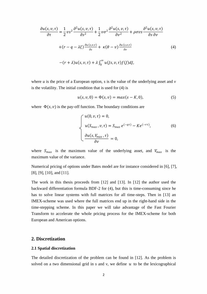
∂𝑢 𝑠, 𝑣, 𝜏
∂𝜏=
1
2𝑣𝑠2
∂2𝑢 𝑠, 𝑣, 𝜏
∂𝑠2+
1
2𝑣𝜍2
∂2𝑢 𝑠, 𝑣, 𝜏
∂𝑣2+ 𝜌𝜍𝑣𝑠
∂2𝑢 𝑠, 𝑣, 𝜏
∂𝑠 ∂𝑣
+ 𝑟 − 𝑞 − 𝜆𝜉 𝜕𝑢 𝑠,𝑣,𝜏
𝜕𝑠+ 𝜅 휃 − 𝑣
𝜕𝑢 𝑠,𝑣,𝜏
𝜕𝑣 (4)
− 𝑟 + 𝜆 𝑢 𝑠, 𝑣, 𝜏 + 𝜆 𝑢 𝐽𝑠, 𝑣, 𝜏 𝑓 𝐽 𝑑𝐽,∞
0
where u is the price of a European option, s is the value of the underlying asset and v
is the volatility. The initial condition that is used for (4) is
𝑢 𝑠, 𝑣, 0 = Ф 𝑠, 𝑣 = 𝑚𝑎𝑥 𝑠 − 𝐾, 0 , (5)
where Ф(𝑠, 𝑣) is the pay-off function. The boundary conditions are
𝑢 0, 𝑣, 𝜏 = 0,
𝑢 𝑆𝑚𝑎𝑥 , 𝑣, 𝜏 = 𝑆𝑚𝑎𝑥 𝑒(−𝑞𝜏) − 𝐾𝑒(−𝑟𝜏), (6)
∂𝑢 𝑠, 𝑉𝑚𝑎𝑥 , 𝜏
∂𝑣 = 0,
where 𝑆𝑚𝑎𝑥 is the maximum value of the underlying asset, and 𝑉𝑚𝑎𝑥 is the
maximum value of the variance.
Numerical pricing of options under Bates model are for instance considered in [6], [7],
[8], [9], [10], and [11].
The work in this thesis proceeds from [12] and [13]. In [12] the author used the
backward differentiation formula BDF-2 for (4), but this is time-consuming since he
has to solve linear systems with full matrices for all time-steps. Then in [13] an
IMEX-scheme was used where the full matrices end up in the right-hand side in the
time-stepping scheme. In this paper we will take advantage of the Fast Fourier
Transform to accelerate the whole pricing process for the IMEX-scheme for both
European and American options.
2. Discretization
2.1 Spatial discretization
The detailed discretization of the problem can be found in [12]. As the problem is
solved on a two dimensional grid in s and v, we define 𝑢 to be the lexicographical
3
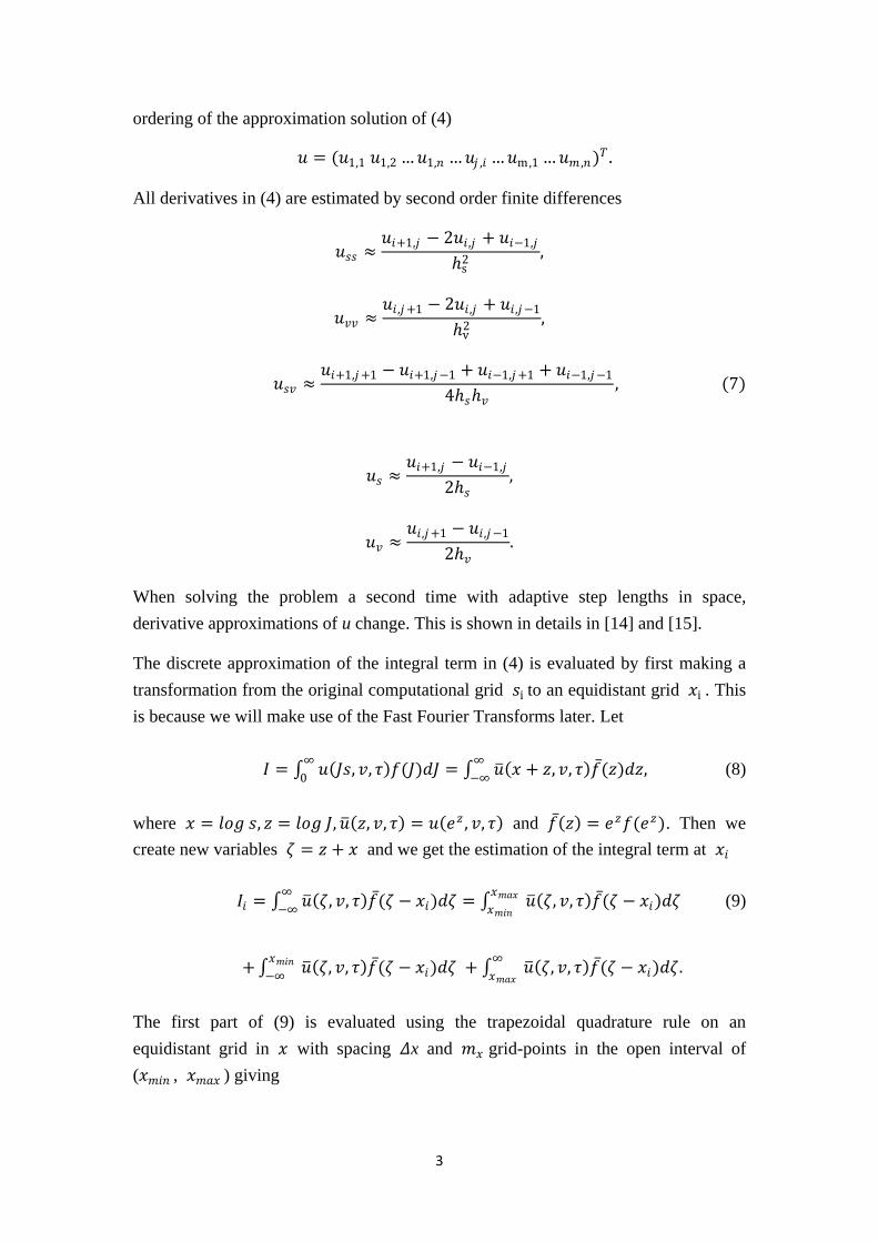
ordering of the approximation solution of (4)
𝑢 = (𝑢1,1 𝑢1,2 … 𝑢1,𝑛 … 𝑢𝑗 ,𝑖 … 𝑢m,1 … 𝑢𝑚 ,𝑛)𝑇 .
All derivatives in (4) are estimated by second order finite differences
𝑢𝑠𝑠 ≈𝑢𝑖+1,𝑗 − 2𝑢𝑖 ,𝑗 + 𝑢𝑖−1,𝑗
s2
,
𝑢𝑣𝑣 ≈𝑢𝑖 ,𝑗 +1 − 2𝑢𝑖 ,𝑗 + 𝑢𝑖 ,𝑗−1
v2
,
𝑢𝑠𝑣 ≈𝑢𝑖+1,𝑗 +1 − 𝑢𝑖+1,𝑗−1 + 𝑢𝑖−1,𝑗 +1 + 𝑢𝑖−1,𝑗−1
4𝑠𝑣, (7)
𝑢𝑠 ≈𝑢𝑖+1,𝑗 − 𝑢𝑖−1,𝑗
2𝑠,
𝑢𝑣 ≈𝑢𝑖 ,𝑗 +1 − 𝑢𝑖 ,𝑗−1
2𝑣.
When solving the problem a second time with adaptive step lengths in space,
derivative approximations of u change. This is shown in details in [14] and [15].
The discrete approximation of the integral term in (4) is evaluated by first making a
transformation from the original computational grid 𝑠i to an equidistant grid 𝑥i . This
is because we will make use of the Fast Fourier Transforms later. Let
𝐼 = 𝑢 𝐽𝑠, 𝑣, 𝜏 𝑓(𝐽)𝑑𝐽∞
0= 𝑢 𝑥 + 𝑧, 𝑣, 𝜏 𝑓 (𝑧)𝑑𝑧
∞
−∞, (8)
where 𝑥 = 𝑙𝑜𝑔 𝑠, 𝑧 = 𝑙𝑜𝑔 𝐽, 𝑢 𝑧, 𝑣, 𝜏 = 𝑢 𝑒𝑧 , 𝑣, 𝜏 and 𝑓 𝑧 = 𝑒𝑧𝑓(𝑒𝑧). Then we
create new variables 휁 = 𝑧 + 𝑥 and we get the estimation of the integral term at 𝑥𝑖
𝐼𝑖 = 𝑢 휁, 𝑣, 𝜏 𝑓 (휁 − 𝑥𝑖)𝑑휁∞
−∞= 𝑢 휁, 𝑣, 𝜏 𝑓 (휁 − 𝑥𝑖)𝑑휁
𝑥𝑚𝑎𝑥
𝑥𝑚𝑖𝑛 (9)
+ 𝑢 휁, 𝑣, 𝜏 𝑓 (휁 − 𝑥𝑖)𝑑휁 𝑥𝑚𝑖𝑛
−∞+ 𝑢 휁, 𝑣, 𝜏 𝑓 (휁 − 𝑥𝑖)𝑑휁
∞
𝑥𝑚𝑎𝑥.
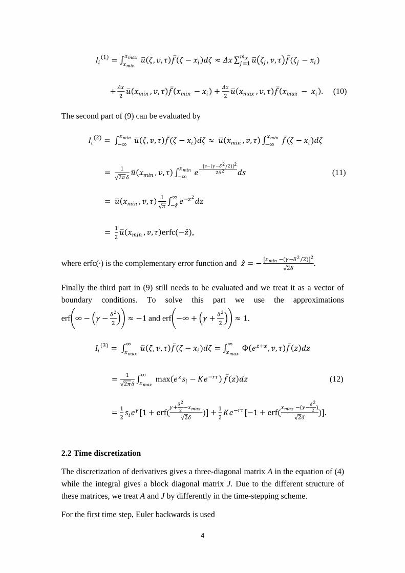
The first part of (9) is evaluated using the trapezoidal quadrature rule on an
equidistant grid in 𝑥 with spacing 𝛥x and 𝑚𝑥 grid-points in the open interval of
(𝑥𝑚𝑖𝑛 , 𝑥𝑚𝑎𝑥 ) giving
4
𝐼𝑖 1 = 𝑢 휁, 𝑣, 𝜏 𝑓 휁 − 𝑥𝑖 𝑑휁
𝑥𝑚𝑎𝑥
𝑥𝑚𝑖𝑛≈ 𝛥𝑥 𝑢 휁𝑗 , 𝑣, 𝜏 𝑓 (휁𝑗 − 𝑥𝑖)
𝑚𝑥𝑗 =1
+𝛥𝑥
2𝑢 𝑥𝑚𝑖𝑛 , 𝑣, 𝜏 𝑓 𝑥𝑚𝑖𝑛 − 𝑥𝑖 +
𝛥𝑥
2𝑢 𝑥𝑚𝑎𝑥 , 𝑣, 𝜏 𝑓 𝑥𝑚𝑎𝑥 − 𝑥𝑖 . (10)
The second part of (9) can be evaluated by
𝐼𝑖(2) = 𝑢 휁, 𝑣, 𝜏 𝑓 (휁 − 𝑥𝑖)𝑑휁
𝑥𝑚𝑖𝑛
−∞≈ 𝑢 𝑥𝑚𝑖𝑛 , 𝑣, 𝜏 𝑓 (휁 − 𝑥𝑖)𝑑휁
𝑥𝑚𝑖𝑛
−∞
= 1
2𝜋𝛿𝑢 𝑥𝑚𝑖𝑛 , 𝑣, 𝜏 𝑒
−[𝑠−(𝛾−𝛿2/2)]2
2𝛿2 𝑑𝑠𝑥𝑚𝑖𝑛
−∞ (11)
= 𝑢 𝑥𝑚𝑖𝑛 , 𝑣, 𝜏 1
𝜋 𝑒−𝑧2
𝑑𝑧 ∞
−𝑧
= 1
2𝑢 𝑥𝑚𝑖𝑛 , 𝑣, 𝜏 erfc(−𝑧 ),
where erfc(∙) is the complementary error function and 𝑧 = −[𝑥𝑚𝑖𝑛 −(𝛾−𝛿2/2)]2
2𝛿.
Finally the third part in (9) still needs to be evaluated and we treat it as a vector of
boundary conditions. To solve this part we use the approximations
erf ∞ − 𝛾 −𝛿2
2 ≈ −1 and erf −∞ + 𝛾 +
𝛿2
2 ≈ 1.
𝐼𝑖(3) = 𝑢 휁, 𝑣, 𝜏 𝑓 (휁 − 𝑥𝑖)𝑑휁
∞
𝑥𝑚𝑎𝑥= Ф 𝑒𝑧+𝑥 , 𝑣, 𝜏 𝑓 𝑧 𝑑𝑧
∞
𝑥𝑚𝑎𝑥
=1
2𝜋𝛿 max 𝑒𝑧𝑠𝑖 − 𝐾𝑒−𝑟𝜏 𝑓 𝑧 𝑑𝑧
∞
𝑥𝑚𝑎𝑥 (12)
=1
2𝑠𝑖𝑒
𝛾 [1 + erf(𝛾+
𝛿2
2−𝑥𝑚𝑎𝑥
2𝛿)] +
1
2𝐾𝑒−𝑟𝜏 [−1 + erf(
𝑥𝑚𝑎𝑥 −(𝛾−𝛿2
2)
2𝛿)].
2.2 Time discretization
The discretization of derivatives gives a three-diagonal matrix A in the equation of (4)
while the integral gives a block diagonal matrix J. Due to the different structure of
these matrices, we treat A and J by differently in the time-stepping scheme.
For the first time step, Euler backwards is used
5
𝑢1 = ∆𝑡(𝐴+𝐽)𝑢1 + 𝑢0, (13)
where ∆𝑡 is the discretization parameter in time.
For the remaining time-steps, the Bates model is solved with an IMEX-scheme.
Specifically, we treat the matrix A implicitly whereas we treat the matrix J explicitly
in the Crank-Nicholson, Adams-Bashforth scheme. The advantage of this
IMEX-scheme is that it is faster than the fully implicit method and more stable than
the pure explicit method.
𝑢𝑘+1 ≈ ∆𝑡𝐴𝑢𝑘+1+𝑢𝑘
2+ ∆𝑡𝐽
3𝑢𝑘−𝑢𝑘−1
2+ 𝑢𝑘 , for k=2,…m-1. (14)
More details about the IMEX method can be found in [16].
3. Fast Fourier Transforms
In order to increase the efficiency of the multiplication by the J matrix and the vector
𝑢, we will use the Fast Fourier Transforms (FFTs).
Let 𝐼 𝑖 = 𝛥𝑥 𝑢 휁𝑗 , 𝑣, 𝜏 𝑓 휁𝑗 − 𝑥𝑖 𝑚𝑥𝑗 =1 in (9) and all 𝐼 𝑖 , i=1,2,… 𝑚𝑥 can be
computed by
𝐼 = 𝑇𝑚𝑥𝑢 , (15)
where 𝐼 = (𝐼 1 𝐼 2 … 𝐼 𝑚𝑥)𝑇, 𝑢 = (𝑢 1 𝑢 2 … 𝑢 𝑚𝑥
)𝑇, and 𝑇𝑚𝑥 is the Toeplitz matrix
𝑇𝑚𝑥=
𝑓 0
𝑓 −𝛥𝑥
𝑓 𝛥𝑥
𝑓 0 ⋯
𝑓 𝑚𝑥 − 1 𝛥𝑥
𝑓 𝑚𝑥 − 2 𝛥𝑥
⋮ ⋮ ⋱ ⋮𝑓 − 𝑚𝑥 − 1 𝛥𝑥 𝑓 − 𝑚𝑥 − 2 𝛥𝑥 ⋯ 𝑓 0
.
As the constant diagonal Toeplitz matrix 𝑇𝑚𝑥 can be embedded into a circulant
matrix 𝐶2𝑚𝑥−1 with the first row c
𝑐 = ( 𝑓 0 𝑓 𝛥𝑥 ⋯ 𝑓 𝑚𝑥 − 1 𝛥𝑥 0 0 … 0 𝑓 − 𝑚𝑥 − 1 𝛥𝑥 ⋯ 𝑓 −𝛥𝑥 ), (16)
we can first compute 𝐼 = 𝐶2𝑚𝑥−1𝑢 ,where 𝑢 = (𝑢 1 𝑢 2 … 𝑢 𝑚𝑥 0 … 0)𝑇 . 𝐼 can then
be achieved by the first 𝑚𝑥 elements in 𝐼 .
To make use of the FFTs, we must first decompose the matrix 𝐶2𝑚𝑥−1 as
𝐶2𝑚𝑥−1 = 𝐹2𝑚𝑥−1−1 𝛬𝐹2𝑚𝑥−1, (17)
where 𝐹2𝑚𝑥−1 is a Fourier matrix of order 2𝑚𝑥 − 1 and 𝛬 is a diagonal matrix
6
with the eigenvalues of 𝐶2𝑚𝑥−1 on the diagonal. Then 𝐼 is given by
𝐼 = 𝐹2𝑚𝑥−1−1 𝛬𝐹2𝑚𝑥−1𝑢 , which could be accomplished by using two fast Fourier
transforms (FFTs) and one inverse fast Fourier transforms (IFFTs). To get an accurate
estimation, we choose to embed 𝑇𝑚𝑥 in a circulant matrix 𝐶𝑀𝑥
where 𝑀𝑥 is the
smallest power of 2 such that 𝑀𝑥 ≥ 2𝑚𝑥 − 1 and the number of grid points in x is
twice as many as those in s. The eigenvalues of 𝐶𝑀𝑥 can be computed once in the
beginning to improve the efficiency.
Generally, the computation of the matrix-vector multiplication in (15) follows the
algorithm below:
Interpolate values to new equidistant points 𝑥𝑖 from the 𝑠𝑖 grid-points in
Section 2.
Compute 𝑇𝑚𝑥 and embed it into a circulant matrix 𝐶𝑀𝑥
.
Use the FFTs above to compute 𝐼 .
Get 𝐼 by taking the first 𝑚𝑥 elements in 𝐼 .
Interpolate values of 𝐼𝑖 back to the original grid-points 𝑠𝑖 .
4. Adaptive method
The purpose of making use of the adaptive method is to place grid-points where they
are most needed for accuracy reasons, [14], [15]. First of all, we need to solve the
problem on a sparse equidistant grid. Then a new, adaptive grid can be constructed
where grid points could be distributed more efficiently. In this paper, we consider
adaptivity in s and v.
The adaptive process in s works like this: (v is treated analogously): Let B be the
“exact” discrete representation of the right hand side of equation (4). For any smooth
solution u, it holds that
𝐵𝑠𝑣𝑢𝑠𝑣
= 𝐵𝑢 + 𝜏𝑠𝑣, (18)
where 𝐵𝑠𝑣𝑢𝑠𝑣
is the discrete approximation in space of (4), 𝑢𝑠𝑣 is the vector
of the numerical solution, and 𝜏𝑠𝑣 is the truncation error of the approximation with
step-lengths 𝑠 and 𝑣. Use the approximation
𝜏𝑠𝑣≈ 𝑠
2휂𝑠 𝑠, 𝑣 + 𝑣2휂𝑣 𝑠, 𝑣 = 𝜏𝑠
+ 𝜏𝑣, (19)
and consider first
7
𝜏𝑠≈ 𝑠
2휂𝑠 𝑠, 𝑣 . (20)
Define
𝛿𝑠= 𝐵𝑢 + 𝜏𝑠
, (21)
𝛿2𝑠= 𝐵𝑢 + 𝜏2𝑠
.
The local discretization error of the approximation of order p on the grid with step
size 𝑠 can be approximated in the coarse grid with the step size 2𝑠 by using (19)
and (20)
𝜏𝑠=
1
3 𝛿2𝑠
− 𝛿𝑠 . (22)
The local truncation error 𝜏𝑠 is computed in several points in time. The maximum
absolute value of 𝜏𝑠 is chosen in each spatial point to calculate the new grid.
In order to get an approximation for 휂𝑠 𝑠, 𝑣 , we compute a solution with a step
length . Then from equation (20), we get
휂𝑠 𝑠, 𝑣 =𝜏 𝑠
(𝑠,𝑣)
𝑠2 . (23)
To control the local discretization error such that 𝜏𝑠 𝑠 ≤ 휀𝑠 for any 휀𝑠>0, we
obtain the following by combining (20) ,(21) and (22)
𝜏𝑠 𝑠 = 𝑠
2 𝑠 휂𝑠 𝑠, 𝑣 ≈ 𝑠2 𝑠
𝜏 𝑠 𝑠,𝑣
𝑠2 𝑠
≤ 휀𝑠 . (24)
Using Equation (25)
𝜏 𝑠 𝑠 = 𝑚𝑎𝑥𝑣 𝜏 𝑠
𝑠, 𝑣 , (25)
we could obtain
𝑠 𝑠 = 𝑠 𝑠 (휀𝑠
𝜏 𝑠 𝑠
)1/2. (26)
To prevent the algorithm from taking too big space-steps in s when the truncation
error is small, we introduce a parameter 𝛾𝑠 to the equation (26)
𝑠 𝑠 = 𝑠 𝑠 (휀𝑠
휀𝑠𝛾𝑠+𝜏 𝑠 𝑠
)1/2. (27)
Finally, a simple linear interpolation could be used to get 𝑠 𝑠 between known
function values.
8
5. American Option Pricing
In this paper, we use the operator splitting method [17] for the pricing of American
options. For simplicity, we introduce the operator
ℒ𝑢 = ∂𝑢 𝑠, 𝑣, 𝜏
∂𝜏−
1
2𝑣𝑠2
∂2𝑢 𝑠, 𝑣, 𝜏
∂𝑠2−
1
2𝑣𝜍2
∂2𝑢 𝑠, 𝑣, 𝜏
∂𝑣2− 𝜌𝜍𝑣𝑠
∂2𝑢 𝑠, 𝑣, 𝜏
∂𝑠 ∂𝑣
− 𝑟 − 𝑞 − 𝜆𝜉 ∂𝑢 𝑠,𝑣,𝜏
∂𝑠− 𝜅 휃 − 𝑣
∂𝑢 𝑠,𝑣,𝜏
∂𝑣 (28)
−𝜆 𝑢 𝐽𝑠, 𝑣, 𝜏 𝑓(𝐽)𝑑𝐽∞
0+ 𝑟 + 𝜆 𝑢 𝑠, 𝑣, 𝜏 .
As American options can be exercised earlier than the maturity date T, we have to
include the following constraint for the option price:
𝑢 𝑠, 𝑣, 𝜏 ≥ Ф 𝑠, 𝑣 , 𝑠 ∈ 0, 𝑆𝑚𝑎𝑥 , 𝑣 ∈ 0, 𝑉𝑚𝑎𝑥 , 𝜏 ∈ 0, 𝑇 . (29)
This gives that the price of the American option based on the Bates model can be
obtained by solving a time dependent linear complementarity problem
ℒ𝑢 ≥ 0, 𝑢 ≥ Ф,
𝑢 − Ф ℒ𝑢 = 0, (30)
for 𝑠, 𝑣, 𝜏 ϵ 0, 𝑆𝑚𝑎𝑥 × 0, 𝑉𝑚𝑎𝑥 × 0, 𝑇 with the initial condition (5) and
boundary conditions
𝑢 0, 𝑣, 𝜏 = 0,
𝑢 𝑆𝑚𝑎𝑥 , 𝑣, 𝜏 = 𝑚𝑎𝑥(𝑆𝑚𝑎𝑥 𝑒(−𝑞𝜏) − 𝐾𝑒(−𝑟𝜏), 𝑆𝑚𝑎𝑥 − 𝐾), (31)
∂𝑢 𝑠, 𝑉𝑚𝑎𝑥 , 𝜏
∂𝑣= 0.
We now present the operator splitting method for the linear complementarity problem
(30) based on the following formulation with an auxiliary variable 𝜆:
ℒ𝑢 = 𝜆,
𝜆 ≥ 0, 𝑢 ≥ Ф, 𝑢 − Ф 𝜆 = 0,
(31)
with the initial condition (5) and boundary conditions (31).
9
By using the same space and time discretizations as in Section 2, the operator splitting
method [17] can be applied based on two fractional time steps. In the first fractional
step, we solve a system of linear equations. Then the solution and the variable 𝜆 are
updated which satisfy the constraints for them in the second step. Since the operator
splitting depends on the underlying time discretization, we describe the operator
splitting methods for Euler backwards and the IMEX scheme.
For the first time step, the operator splitting method for the implicit Euler scheme
reads
1
∆𝑡𝑰 − 𝑨 + 𝑱 𝒖 𝑘+1 =
1
∆𝑡𝐼 𝒖𝑘 + 𝝀𝑘 , (33)
1
∆𝑡 𝒖𝑘+1 − 𝒖 𝑘+1 − 𝝀𝑘+1 − 𝝀𝑘 = 0,
(𝝀𝑘+1)𝑇 𝒖𝑘+1 − 𝒈 = 0, 𝒖𝑘+1 ≥ 𝒈 𝐚𝐧d 𝝀𝑘+1 ≥ 0, (34)
for k=1. The solution 𝒖 𝑘+1 of the linear system of equations (33) is obtained and
updates for 𝝀𝑘+1 and 𝒖𝑘+1 by using Equations (34).
Then for the time step k= 2,3,…m-1, the operator splitting for IMEX scheme reads
1
∆𝑡𝑰 −
1
2𝑨 𝒖 𝑘+1 =
1
∆𝑡𝑰 +
1
2𝑨 +
3
2𝑱 𝒖𝑘 −
1
2𝑱𝒖𝑘−1 + 𝝀𝑘 , (35)
1
∆𝑡 𝒖𝑘+1 − 𝒖 𝑘+1 − 𝝀𝑘+1 − 𝝀𝑘 = 0,
(𝝀𝑘+1)𝑇 𝒖𝑘+1 − 𝒈 = 0, 𝒖𝑘+1 ≥ 𝒈 𝐚𝐧d 𝝀𝑘+1 ≥ 0. (36)
Again, the solution 𝒖 𝑘+1 is achieved by solving (35) and updates are performed
using Equation (36).
6. Numerical results
In this section we present some computational results for European options and
American options using equidistant and adaptive grids.
The implementation is done in MATLAB and the matrix A is allocated as a sparse
matrix. The linear system of equations obtained from Euler backwards and the
IMEX-scheme are solved by the iterative method Generalized Minimal Residual
Method (GMRES), see [19]. We restart GMRES after six iterations for efficiency.
When the residual is smaller than 10−8 , we terminate the iteration process.
10
MATLAB’s built-in, sparse, incomplete LU factorization, ilu has been used as a
preconditioner. To improve the efficiency, we only need to calculate L and U once for
Euler backwards and once again for the IMEX-scheme.
Parameters are chosen as follows: risk free interest rate 𝑟 = 0.03, the dividend yield
𝑞 = 0.05, the strike price 𝐾 = 100, the maturity date T = 0.5, the correlation
between the two Wiener processes 𝜌 = −0.5, the mean level of variance 휃 = 0.04,
the rate of reversion 𝜅 = 2.0, the volatility of the variance 𝜍 = 0.25, the intensity
rate of the jump 𝜆 = 0.2, the parameters of mean and variance of the jump 𝛾 and 𝛿
are −0.5 and 0.4 respectively. We use the rule of thumb, 𝑆𝑚𝑎𝑥 = 4𝐾, 𝑆𝑚𝑖𝑛 = 0,
and 𝑉𝑚𝑎𝑥 =1.
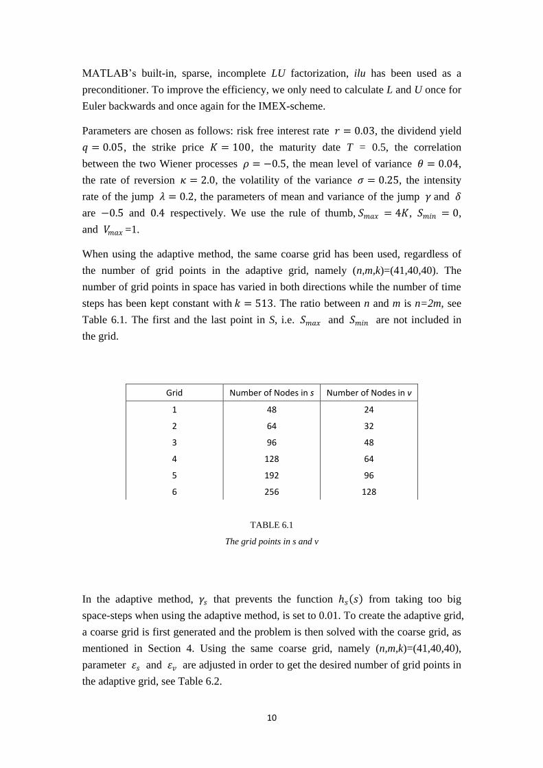
When using the adaptive method, the same coarse grid has been used, regardless of
the number of grid points in the adaptive grid, namely (n,m,k)=(41,40,40). The
number of grid points in space has varied in both directions while the number of time
steps has been kept constant with 𝑘 = 513. The ratio between n and m is n=2m, see
Table 6.1. The first and the last point in S, i.e. 𝑆𝑚𝑎𝑥 and 𝑆𝑚𝑖𝑛 are not included in
the grid.
TABLE 6.1
The grid points in s and v
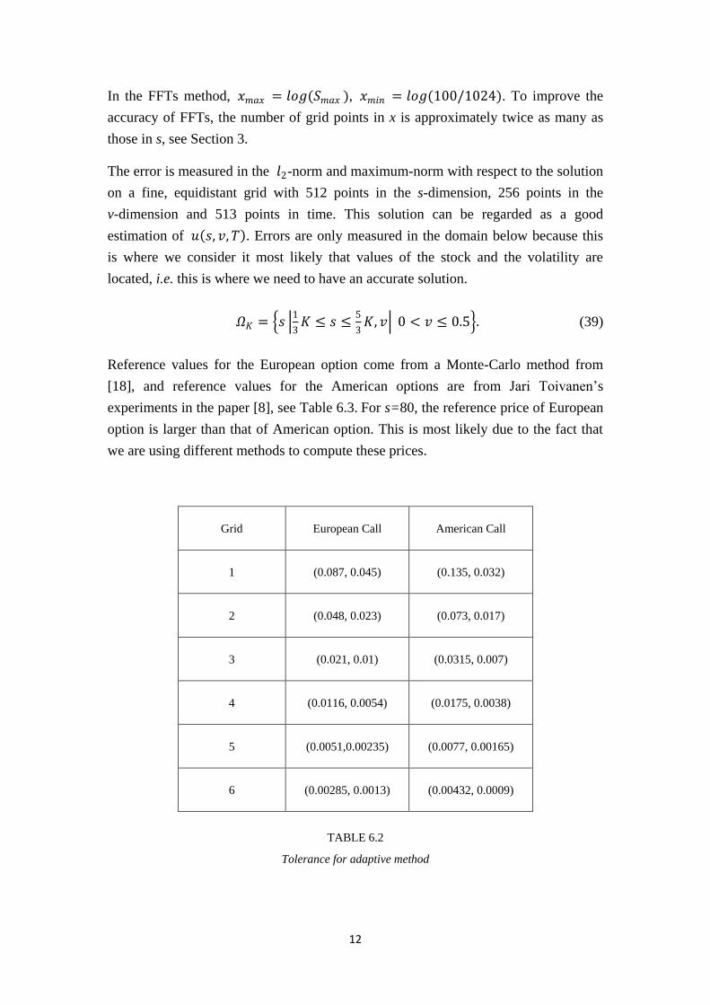
In the adaptive method, 𝛾𝑠 that prevents the function 𝑠 𝑠 from taking too big
space-steps when using the adaptive method, is set to 0.01. To create the adaptive grid,
a coarse grid is first generated and the problem is then solved with the coarse grid, as
mentioned in Section 4. Using the same coarse grid, namely (n,m,k)=(41,40,40),
parameter 휀𝑠 and 휀𝑣 are adjusted in order to get the desired number of grid points in
the adaptive grid, see Table 6.2.
Grid Number of Nodes in s Number of Nodes in v
1
2
3
4
5
6
48
64
96
128
192
256
24
32
48
64
96
128
11
K
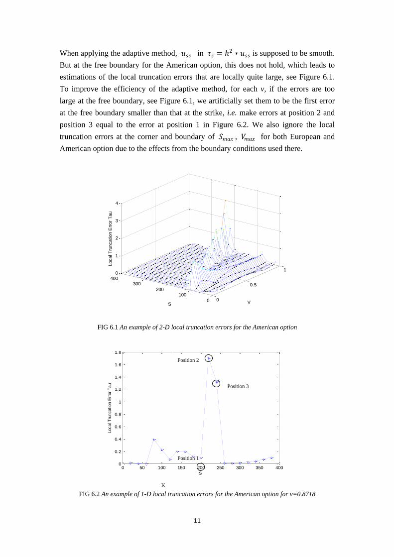
When applying the adaptive method, 𝑢𝑠𝑠 in 𝜏𝑠 = 2 ∗ 𝑢𝑠𝑠 is supposed to be smooth.
But at the free boundary for the American option, this does not hold, which leads to
estimations of the local truncation errors that are locally quite large, see Figure 6.1.
To improve the efficiency of the adaptive method, for each v, if the errors are too
large at the free boundary, see Figure 6.1, we artificially set them to be the first error
at the free boundary smaller than that at the strike, i.e. make errors at position 2 and
position 3 equal to the error at position 1 in Figure 6.2. We also ignore the local
truncation errors at the corner and boundary of 𝑆𝑚𝑎𝑥 , 𝑉𝑚𝑎𝑥 for both European and
American option due to the effects from the boundary conditions used there.
FIG 6.1 An example of 2-D local truncation errors for the American option
FIG 6.2 An example of 1-D local truncation errors for the American option for v=0.8718
0
0.5
1
0
100200
300400
0
1
2
3
4
VS
Local T
runcation E
rror
Tau
0 50 100 150 200 250 300 350 4000
0.2
0.4
0.6
0.8
1
1.2
1.4
1.6
1.8
S
Local T
runcation E
rror
Tau
Position 1
Position 3
Position 2
12
In the FFTs method, 𝑥𝑚𝑎𝑥 = 𝑙𝑜𝑔(𝑆𝑚𝑎𝑥 ), 𝑥𝑚𝑖𝑛 = 𝑙𝑜𝑔(100/1024). To improve the
accuracy of FFTs, the number of grid points in x is approximately twice as many as
those in s, see Section 3.
The error is measured in the 𝑙2-norm and maximum-norm with respect to the solution
on a fine, equidistant grid with 512 points in the s-dimension, 256 points in the
v-dimension and 513 points in time. This solution can be regarded as a good
estimation of 𝑢 𝑠, 𝑣, 𝑇 . Errors are only measured in the domain below because this
is where we consider it most likely that values of the stock and the volatility are
located, i.e. this is where we need to have an accurate solution.
𝛺𝐾 = 𝑠 1
3𝐾 ≤ 𝑠 ≤
5
3𝐾, 𝑣 0 < 𝑣 ≤ 0.5 . (39)
Reference values for the European option come from a Monte-Carlo method from
[18], and reference values for the American options are from Jari Toivanen’s
experiments in the paper [8], see Table 6.3. For s=80, the reference price of European
option is larger than that of American option. This is most likely due to the fact that
we are using different methods to compute these prices.
TABLE 6.2
Tolerance for adaptive method
Grid European Call American Call
1 (0.087, 0.045) (0.135, 0.032)
2 (0.048, 0.023) (0.073, 0.017)
3 (0.021, 0.01) (0.0315, 0.007)
4 (0.0116, 0.0054) (0.0175, 0.0038)
5 (0.0051,0.00235) (0.0077, 0.00165)
6 (0.00285, 0.0013) (0.00432, 0.0009)
13
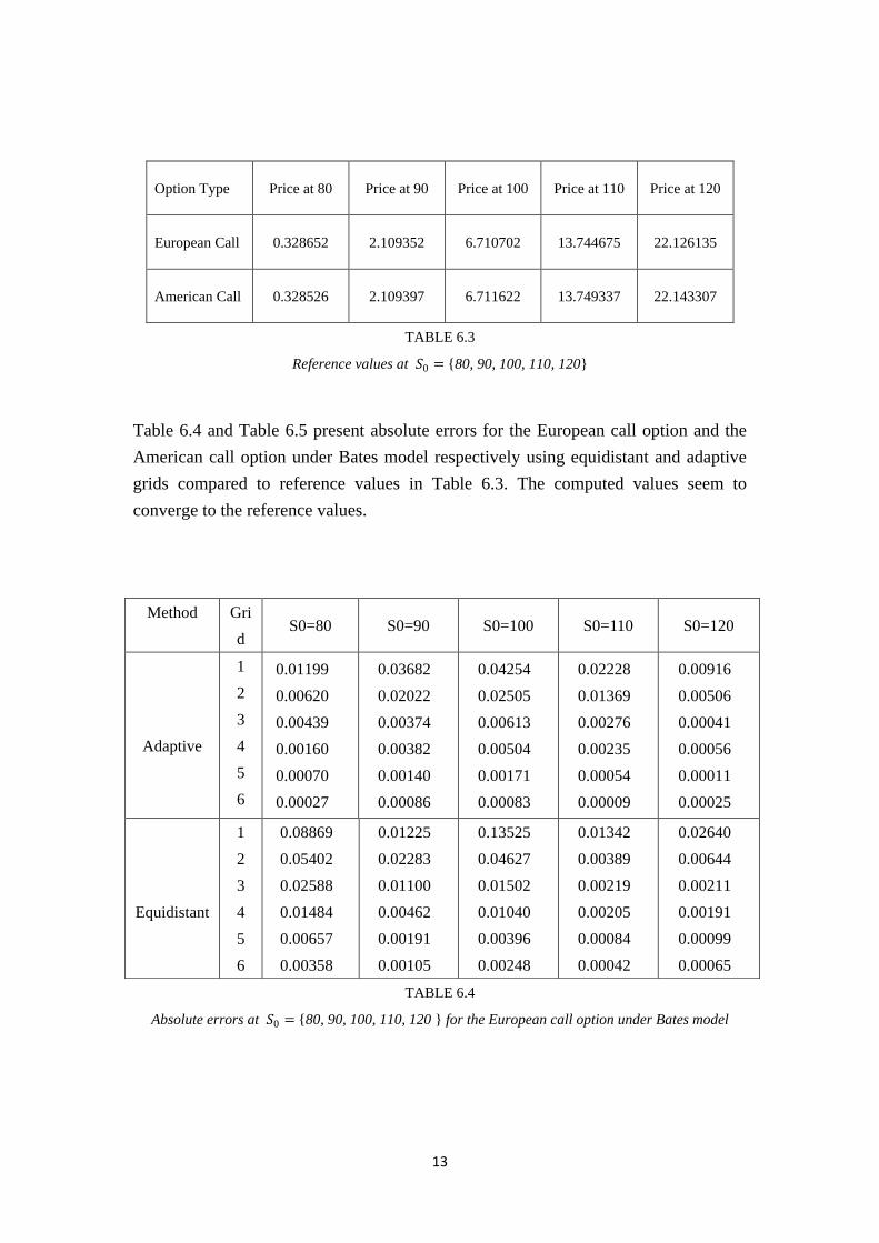
TABLE 6.3
Reference values at 𝑆0 = {80, 90, 100, 110, 120}
Table 6.4 and Table 6.5 present absolute errors for the European call option and the
American call option under Bates model respectively using equidistant and adaptive
grids compared to reference values in Table 6.3. The computed values seem to
converge to the reference values.
TABLE 6.4
Absolute errors at 𝑆0 = {80, 90, 100, 110, 120 } for the European call option under Bates model
Option Type Price at 80 Price at 90 Price at 100 Price at 110 Price at 120
European Call 0.328652 2.109352 6.710702 13.744675 22.126135
American Call 0.328526 2.109397 6.711622 13.749337 22.143307
Method Gri
d S0=80 S0=90 S0=100 S0=110 S0=120
Adaptive
1
2
3
4
5
6
0.01199
0.00620
0.00439
0.00160
0.00070
0.00027
0.03682
0.02022
0.00374
0.00382
0.00140
0.00086
0.04254
0.02505
0.00613
0.00504
0.00171
0.00083
0.02228
0.01369
0.00276
0.00235
0.00054
0.00009
0.00916
0.00506
0.00041
0.00056
0.00011
0.00025
Equidistant
1
2
3
4
5
6
0.08869
0.05402
0.02588
0.01484
0.00657
0.00358
0.01225
0.02283
0.01100
0.00462
0.00191
0.00105
0.13525
0.04627
0.01502
0.01040
0.00396
0.00248
0.01342
0.00389
0.00219
0.00205
0.00084
0.00042
0.02640
0.00644
0.00211
0.00191
0.00099
0.00065
14
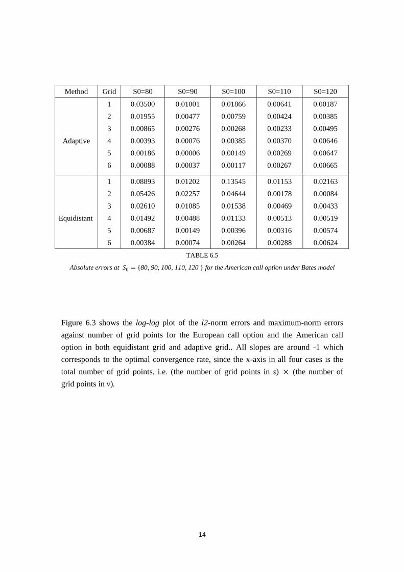
TABLE 6.5
Absolute errors at 𝑆0 = {80, 90, 100, 110, 120 } for the American call option under Bates model
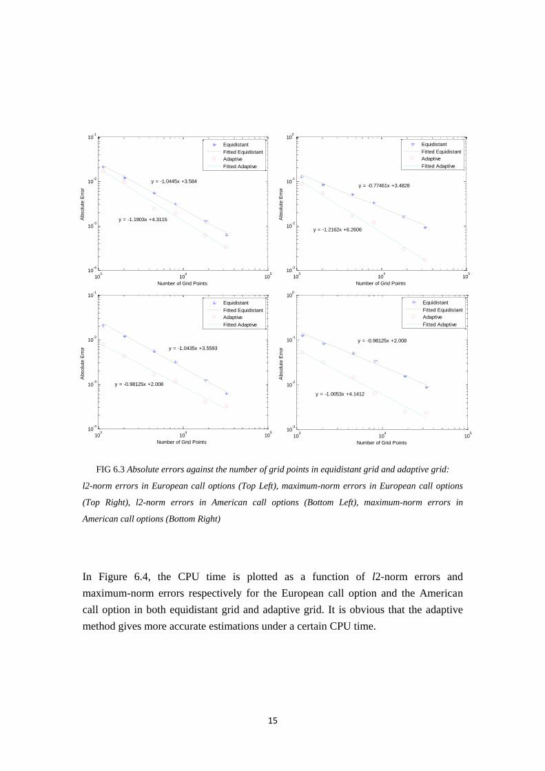
Figure 6.3 shows the log-log plot of the l2-norm errors and maximum-norm errors
against number of grid points for the European call option and the American call
option in both equidistant grid and adaptive grid.. All slopes are around -1 which
corresponds to the optimal convergence rate, since the x-axis in all four cases is the
total number of grid points, i.e. (the number of grid points in s) × (the number of
grid points in v).
Method Grid S0=80 S0=90 S0=100 S0=110 S0=120
Adaptive
1
2
3
4
5
6
0.03500
0.01955
0.00865
0.00393
0.00186
0.00088
0.01001
0.00477
0.00276
0.00076
0.00006
0.00037
0.01866
0.00759
0.00268
0.00385
0.00149
0.00117
0.00641
0.00424
0.00233
0.00370
0.00269
0.00267
0.00187
0.00385
0.00495
0.00646
0.00647
0.00665
Equidistant
1
2
3
4
5
6
0.08893
0.05426
0.02610
0.01492
0.00687
0.00384
0.01202
0.02257
0.01085
0.00488
0.00149
0.00074
0.13545
0.04644
0.01538
0.01133
0.00396
0.00264
0.01153
0.00178
0.00469
0.00513
0.00316
0.00288
0.02163
0.00084
0.00433
0.00519
0.00574
0.00624
15
FIG 6.3 Absolute errors against the number of grid points in equidistant grid and adaptive grid:
l2-norm errors in European call options (Top Left), maximum-norm errors in European call options
(Top Right), l2-norm errors in American call options (Bottom Left), maximum-norm errors in
American call options (Bottom Right)
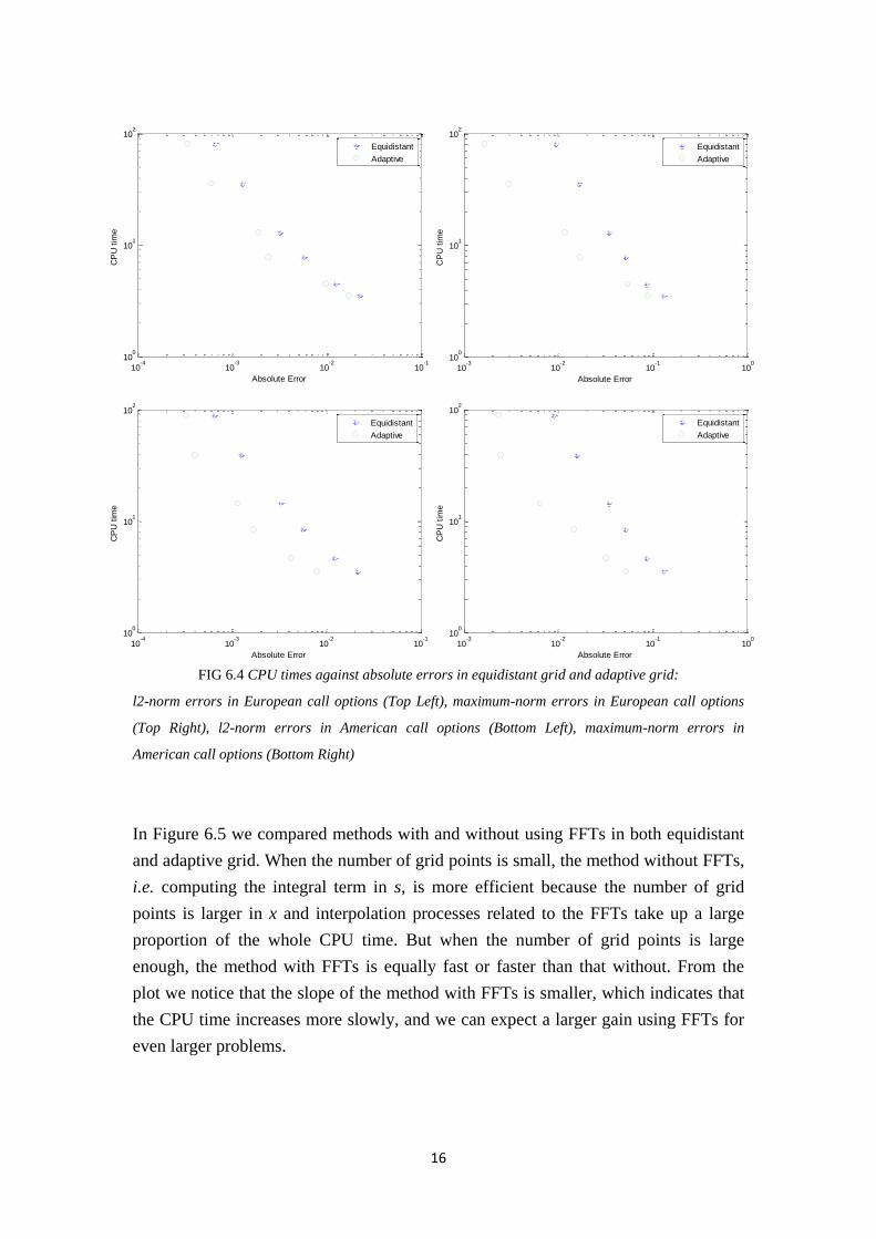
In Figure 6.4, the CPU time is plotted as a function of l2-norm errors and
maximum-norm errors respectively for the European call option and the American
call option in both equidistant grid and adaptive grid. It is obvious that the adaptive
method gives more accurate estimations under a certain CPU time.
103
104
105
10-4
10-3
10-2
10-1
Number of Grid Points
Absolu
te E
rror
Equidistant
Fitted Equidistant
Adaptive
Fitted Adaptive
y = -1.0445x +3.584
y = -1.1903x +4.3115
103
104
105
10-3
10-2
10-1
100
Number of Grid PointsA
bsolu
te E
rror
y = -0.77461x +3.4828y = -1.2162x +6.2606
Equidistant
Fitted Equidistant
Adaptive
Fitted Adaptive
y = -0.77461x +3.4828
y = -1.2162x +6.2606
103
104
105
10-4
10-3
10-2
10-1
Number of Grid Points
Absolu
te E
rror
Equidistant
Fitted Equidistant
Adaptive
Fitted Adaptive
y = -0.98125x +2.008
y = -1.0435x +3.5593
103
104
105
10-3
10-2
10-1
100
Number of Grid Points
Absolu
te E
rror
Equidistant
Fitted Equidistant
Adaptive
Fitted Adaptive
y = -0.98125x +2.008
y = -1.0053x +4.1412
16
FIG 6.4 CPU times against absolute errors in equidistant grid and adaptive grid:
l2-norm errors in European call options (Top Left), maximum-norm errors in European call options
(Top Right), l2-norm errors in American call options (Bottom Left), maximum-norm errors in
American call options (Bottom Right)
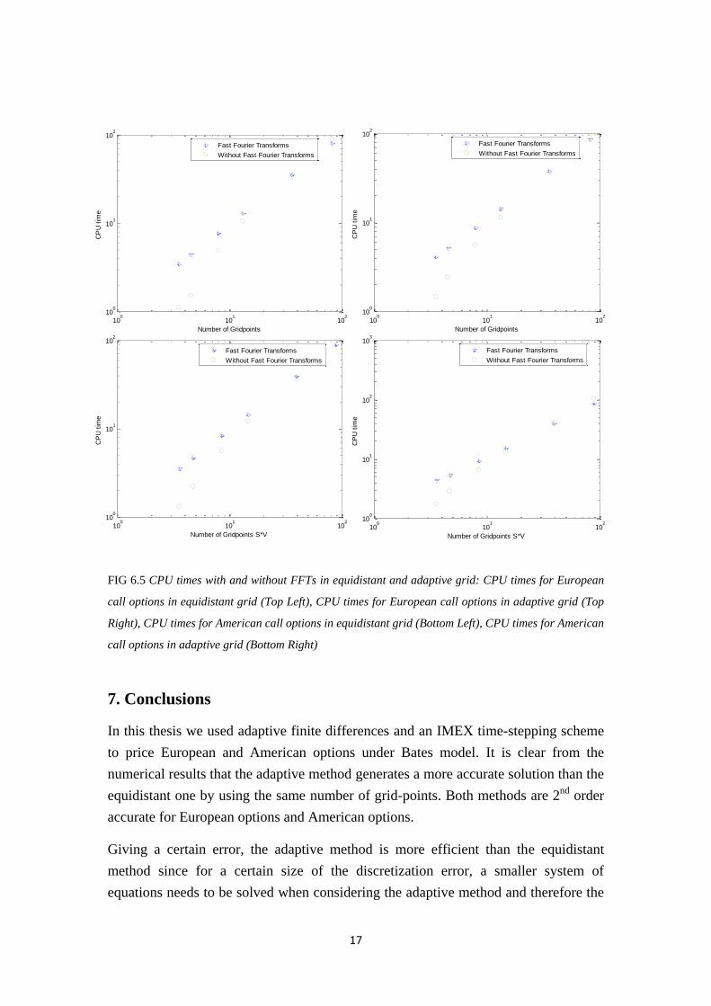
In Figure 6.5 we compared methods with and without using FFTs in both equidistant
and adaptive grid. When the number of grid points is small, the method without FFTs,
i.e. computing the integral term in s, is more efficient because the number of grid
points is larger in x and interpolation processes related to the FFTs take up a large
proportion of the whole CPU time. But when the number of grid points is large
enough, the method with FFTs is equally fast or faster than that without. From the
plot we notice that the slope of the method with FFTs is smaller, which indicates that
the CPU time increases more slowly, and we can expect a larger gain using FFTs for
even larger problems.
10-4
10-3
10-2
10-1
100
101
102
Absolute Error
CP
U t
ime
Equidistant
Adaptive
10-3
10-2
10-1
100
100
101
102
Absolute Error
CP
U t
ime
Equidistant
Adaptive
10-4
10-3
10-2
10-1
100
101
102
Absolute Error
CP
U t
ime
Equidistant
Adaptive
10-3
10-2
10-1
100
100
101
102
Absolute Error
CP
U t
ime
Equidistant
Adaptive
17
FIG 6.5 CPU times with and without FFTs in equidistant and adaptive grid: CPU times for European
call options in equidistant grid (Top Left), CPU times for European call options in adaptive grid (Top
Right), CPU times for American call options in equidistant grid (Bottom Left), CPU times for American
call options in adaptive grid (Bottom Right)
7. Conclusions
In this thesis we used adaptive finite differences and an IMEX time-stepping scheme
to price European and American options under Bates model. It is clear from the
numerical results that the adaptive method generates a more accurate solution than the
equidistant one by using the same number of grid-points. Both methods are 2nd
order
accurate for European options and American options.
Giving a certain error, the adaptive method is more efficient than the equidistant
method since for a certain size of the discretization error, a smaller system of
equations needs to be solved when considering the adaptive method and therefore the
100
101
102
100
101
102
Number of Gridpoints
CP
U t
ime
Fast Fourier Transforms
Without Fast Fourier Transforms
100
101
102
100
101
102
Number of Gridpoints
CP
U t
ime
Fast Fourier Transforms
Without Fast Fourier Transforms
100
101
102
100
101
102
Number of Gridpoints S*V
CP
U t
ime
Fast Fourier Transforms
Without Fast Fourier Transforms
100
101
102
100
101
102
103
Number of Gridpoints S*V
CP
U t
ime
Fast Fourier Transforms
Without Fast Fourier Transforms

18
CPU time is reduced.
Using FFTs in the computation of the integrals is more efficient than standard
matrix-vector multiplication for both European and American option pricing if we
solve large problems.
19
References
[1] F. Black and M. Scholes, The pricing of options and corporate liabilities,
J. Political Economy, 81 (1973), pp. 637-654.
[2] R. C. Merton, Theory of rational option pricing, Bell J. Econom. Management Sci.,
4 (1973), pp. 141-183.
[3] R. C. Merton, Option pricing when underlying stock returns are discontinuous,
Journal of financial economics, 3(1976), pp. 125–144.
[4] S. Heston, A closed-form solution for options with stochastic volatility with
applications to bond and currency options, Rev. Financial Stud., 6 (1993),
pp. 327-343.
[5] D. S. Bates, Jumps and stochastic volatility: Exchange rate processes implicit
Deutsche mark options, Review Financial Stud., 9 (1996), pp. 69-107.
[6] L. V. Ballestra and C. Sgarra, The evaluation of American options in a stochastic
volatility model with jumps: an efficient finite element approach, Comput. Math.
Appl., 60 (2010), pp. 1571-1590.
[7] C. Chiarella, B. Kang, G. H. Meyer, and A. Ziogas, The evaluation of American
option prices under stochastic volatility and jump-diffusion dynamics using the
method of lines, Int. J. Theor. Appl. Finance, 12 (2009), pp. 393-425.
[8] J. Toivanen, A componentwise splitting method for pricing American options
under the Bates model, in Applied and Numerical Partial Differential Equations,
Comput. Methods Appl. Sci. 15, Springer, New York, 2010, pp. 213–227.
[9] E. Miglio and C. Sgarra, A finite element discretization method for option pricing
with the Bates model, SeMA J., 55 (2011), pp. 23–40.
[10] S. Salmi, J. Toivanen, and L. von Sydow, Iterative methods for pricing American
options under the Bates model, in Proceedings of the 2013 International
Conference on Computational Science, Procedia Computer Science Series 18,
Elsevier, Amsterdam, 2013, pp. 1136–1144.
[11] N. Rambeerich, D. Y. Tangman, M. R. Lollchund, and M. Bhuruth, High-order
computational methods for option valuation under multifactor models, European J.
Oper. Res., 224 (2013), pp. 219–226.
[12] A. Sjöberg, Adaptive finite differences to price European options under the Bates
model, IT Report 13063, Department of Information Technology, Uppsala
University, 2013.
[13] A. Westlund, An IMEX-method for pricing options under Bates model using
adaptive finite differences, Department of Information Technology, Uppsala
University, 2014.
20
[14] J. Persson and L. von Sydow, Pricing European multi-asset options using a
space-time adaptive FD-method, Comput. Vis. Sci., 10 (2007), pp. 173-183.
[15] J. Persson and L. von Sydow, Pricing American options using a space-time
adaptive finite difference method, Mathematics and Computers in Simulation,
80(2010), pp. 1922-1935.
[16] S. Salmi and J. Toivanen, Robust and efficient IMEX schemes for option pricing
under jump-diffusion models, Appl. Num. Math, 84(2014), pp. 33-45.
[17] S. Ikonen and J. Toivanen, Operator splitting method for American options with
stochastic volatility, European Congress on Computational Methods in Applied
Sciences and Engineering, ECCOMAS 2004.
[18] J. Toivanen, Private communication, KME, Stanford University, e-mail:
[19] Y. Saad and M. H. Schultz, GMRES: A generalized minimal residual
algorithm for solving nonsymmetric linear systems, SIAM Journal on scientific
and statistical computing, 7(1986), pp. 856-869.