Embed Size (px)
Citation preview
Potassium(I) in waterfrom Theoretical Calculations
Maria RudbeckU.U.D.M. Project Report 2006:9
Examensarbete i matematik, 20 poäng
Handledare: Daniel Spånberg, Institutionen för materialkemioch Lars-Erik Persson, Matematiska institutionen
Examinator: Lars-Erik Persson
Oktober 2006
Department of Mathematics
Uppsala University

Abstract The optimized geometry and energy for [K(H2O)n=1-8]+ clusters have been studied using different
basis sets and different methods (HF, MP2(FULL), BLYP and B3LYP). Moreover, two analytical potentials
have been developed for potassium in water based on MP2(FULL) and B3LYP computations using the 6-
311g* for potassium and the aug-cc-pVTZ(H2O) basis set for water. Two molecular dynamics simulations
have been performed using the potentials, separately, together with a polarizable water potential. The
simulation using both models show that the local water structure in both the first and second solvation shell
of the ion is flexible. The distribution of the coordination numbers for both the models is wide (5-12) and the
average coordination number higher for the model based on the MP2(FULL) calculations (8.1) than for the
model based on B3LYP calculations (6.5). This difference can mostly be explained by differences in K+-
(H2O)n binding energies for the two methods, as well as the fact that the water model was developed using
MP2.

“If it is true that every theory must be based upon observed facts, it is equally true that facts can not be observed without the guidance of some theory. Without such guidance, our facts would be desultory and fruitless; we could not retain them: for the most part we could not even perceive them.”
(Comte, A. (1974 reprint). The positive philosophy of Auguste Comte freely translated and condensed by Harriet Martineau. New York, NY: AMS Press. (Original work published in 1855, New York, NY: Calvin Blanchard, p. 27.)
”Every attempt to employ mathematical methods in the study of chemical questions must be considered profoundly irrational and contrary to the spirit of chemistry. If mathematical analysis would ever hold a prominent place in chemistry – an aberration which is happily almost impossible - it would occasion a rapid and widespread degeneration of that science”
Auguste Comte, 1830.
Contents
1. Introduction
2. Theory
2.1 Quantum Mechanics
2.1.1 Basis sets
2.1.2 Hartree-Fock Theory
2.1.3 Many-Body Perturbation Theory
2.1.4 Coupled Cluster Theory
2.1.5 Density Functional Theory
2.1.6 Hybrid Hartree-Fock/Density Functional Theory
2.1.7 Time versus Accuracy
2.1.8 Counterpoise Basis Set Superposition Error Correction
2.2 Molecular Dynamics
2.2.1 Ensembles
2.2.2 The Potential Energy
2.2.3 Periodic Boundary Conditions
2.2.4 Long-Range Forces
2.2.5 Equations of Motion
2.2.6 Constraint Dynamics
3. Methods
3.1 Quantum Mechanical Calculations
3.1.1 Selection of Methods and Basis Sets
3.1.2 Optimization of [K(H2O)2-8]+
3.1.2 The Potential Energy Curve
3.1.4 Fitting the Potential Energy Curve to the Analytical Potential
3.2 Molecular Dynamical Simulations
3.2.1 Simulation Protocol
3.2.2 Analysis of Molecular Dynamic Simulation Results
4. Results and Discussion
4.1 Quantum Mechanical Results
4.1.1 Selection of Methods and Basis Sets
4.1.2 Optimization of [K(H2O)2-8]+
4.1.3 The Potential Energy Curve
4.1.4 Fitting the Potential Energy Curve to the Analytical Potential
4.2 Molecular Dynamical Results
5. Conclusions
6. Acknowledgment
7. References
8. Appendix I-II
1
1. Introduction
Auguste Comte, often called the father of sociology, named himself the Pope of Positivism. If he was alive
today he would probably be even an inch happier - since mathematical methods are now employed in
chemical questions contrary to his rather sombre prediction (see the pretext). However, theoretical
descriptions need to be handled with great care since small inaccuracies, in energy for instance, can give
large differences in the calculated chemical properties. In order to be “within chemical accuracy” the energy
needs to lie within 1-2 kcal/mol of the true values. The goal of this thesis was to study the structural
properties of the potassium ion in water, an ion which is not only used in alkali batteries and as a fertilizer
[1] but is probably best known for its activities in the plasma membrane in the human cells [2] – a feature
which was acknowledged with two Nobel prizes in chemistry 1991 and 2003. It is already known that the
potassium ion's radius is greater than the sodium ion - but are more water molecules coordinated to the
potassium ion in an aqueous solution? Numerous X-ray and neutron diffraction studies have been performed
for aqueous K+-solutions at different concentrations; see for example the review article by Ohtaki and Radnai
from 1993 [3]. Since the bond length between a potassium ion and a water molecule is close to the bond
length between two water molecules, the hydration structure of the ion is very difficult to measure using the
diffraction methods. Therefore the studies have a large spread ranging from 4 to 8 in coordination number.
EXAFS studies [4] have the advantage over normal X-ray diffraction methods that it has a high selectivity of
the central elements and therefore the K+/H2O distances are completely decoupled from the H2O/H2O
distances. However, the method is also less reliable with respect to the coordination number and therefore
the large spread in the coordination number still exists. In this thesis, properties such as the coordination
number of potassium in water and how the solvated ion fits into bulk water was studied theoretically using
the theories quantum mechanics (QM) and molecular dynamics (MD).
The theory of QM was derived in the beginning of the 20th century and is based on all properties of a system
being fully obtainable from the wave function. The wave function is obtained by solving the Schrödinger
equation – an equation which can only be solved exactly for very simple problems involving no more than
two particles, but it can be solved approximately for many-body systems. The methods employed in this
thesis all assume that the solution of the wave function of the electrons and the wave function of the nuclei
can be separated, due to the large mass difference, the so-called Born-Oppenheimer approximation. Three of
the methods, the ab initio, the Density Functional Theory (DFT) and the hybrid Hartree-Fock (HF)/DFT,
assume that the location of the nuclei is fixed and that the properties of a system is obtained from the
electronic wave function. Within the three basic theories, a number of subdivisions exist - five of which were
employed in this thesis and are described in the theory section.
Due to the time consumption and computational expense, QM is not an ideal tool when studying large
systems including 100s of molecules. Classical molecular dynamics (MD) is a method which also employs
the Born-Oppenheimer approximation but follows the time evolution of the nuclei. The theory is developed
2

using classical mechanics and is solved through Newtons' equations of motion. Just like QM, MD is
branched into a range of methods - in this thesis classical MD was performed where the particle interactions
were described using an analytical potential. The analytical potential was derived through fitting a potential
expression to QM calculations, contrary to the most common approach used in the literature, namely fitting
to a small set of experimental data.
The main focus of this thesis was the optimizations and potential energy calculations of clusters
[K(H2O)n=1-8]+ using QM, the fitting of an analytical potential to the QM computations and finally the MD
simulations. Subsequently, the simulations were analyzed with respect to the coordination number and the
orientation of the water molecules surrounding the potassium in the first and second solvation shells.
3
2. Theory
Quantum Mechanics (QM) and Molecular Dynamics are two complementary techniques: In this thesis, the
QM was considered time-independent and only the electronic degrees of freedom were taken into
consideration, while the MD was time-dependent and only took the motion of the nuclei into account
explicitly. The more computational expensive but more accurate QM was used in order to study smaller
systems while MD was used for the larger systems. Below is a short summary of the two techniques. It
should be noted that the QM energy has been abbreviated with E while the energy used in the MD simulation
has been abbreviated with U in this thesis.
2.1. Quantum Mechanics
In classical mechanics, the motion of matter is described by Newtons' three equations of motion – the total
energy is constant in the absence of external forces, the response of the particles when the forces are acting
on them and that to every action there is an equal and opposite reaction. Quantum mechanics (QM) is used
when the three equations fail to describe light particles, such as electrons, and suggests that a particle can be
described as a wave rather than a finite object traveling along a definitive path. In other words, in QM the
dynamical properties are expressed by a wavefunction which can be obtained by solving the Schrödinger
equation. The Schrödinger equation was proposed by the Austrian physicist Erwin Schrödinger 1926 and its
time-independent form is shown in equation 2.1.
H=E (2.1)
where
H=−ℏ2
2m∇2V (2.2)
and
∇ 2=2
x22
y22
z2 (2.3)
for a three-dimensional system.
Since the Schrödinger equation cannot be solved exactly for many-body systems, a first step in the treatment
is the Born-Oppenheimer approximation, which states that the nuclei can be considered stationary compared
to the electrons due to the large relative mass. This approximation allows the Schrödinger equation to be
written as a product of two wave functions – one for the electronic part and one for the nuclei (see equation
2.4). Since the wave function for the nuclei is in this case considered fixed, it can be assumed to be a
constant at arbitrary locations and be computed using classical mechanics.
tot nuclei , electrons=electronsnuclei (2.4)
4
Apart from the Born-Oppenheimer approximation other approximations need to be adopted in order to solve
the equation. Four different strategies to solve the Schrödinger equation are discussed below in sections
2.1.2-2.1.5. A more detailed description of the methods can be found in the references 5 and 6. Some of the
methods use the variation theory which says that the energy corresponding to an arbitrary wave function is
never less than the true energy - consequently the best function corresponds to the minimum in energy. Other
methods use the perturbation theory which aims to find an easier computed but related problem and then
considers how the difference between the real and simpler problems affects the solution. The perturbation
theory is very useful when the difference between the two problems is small.
2.1.1 Basis sets
Atomic orbitals describe where an electron may be found in a single atom whereas the molecular orbitals
describes where an electron may be found in a molecule. Each molecular orbital is commonly, and in the
methods employed, expressed as a linear combination of atomic orbitals (LCAO), i.e. atomic-like functions
are used as basis sets, see equation 2.5.
i=∑v=1
K
cviv (2.5)
The most natural way to describe the atomic orbitals is through Slater type orbitals, STO, since these are the
exact solutions of the Schrödinger equation for the hydrogen atom, see equation 2.5. However, when solving
the Schrödinger equation for many-electron systems, integrals of products of the basis functions are required.
Since the calculations can be very expensive, the STO:s are often replaced with Gaussian type orbitals,
GTO:s (see equation 2.7). The advantage with the GTO:s is that the product of two orbitals can be expressed
as one, see equation 2.8.
x h yk z l e− r (2.6)
x h yk z l e− r 2
(2.7)
Aa e−a ra2
⋅Ab e−b rb2
=Ac e−c rc2
(2.8)
where α is a radial extent and the sum of the Cartesian variables h, k and l determines the order of the
Gaussian.
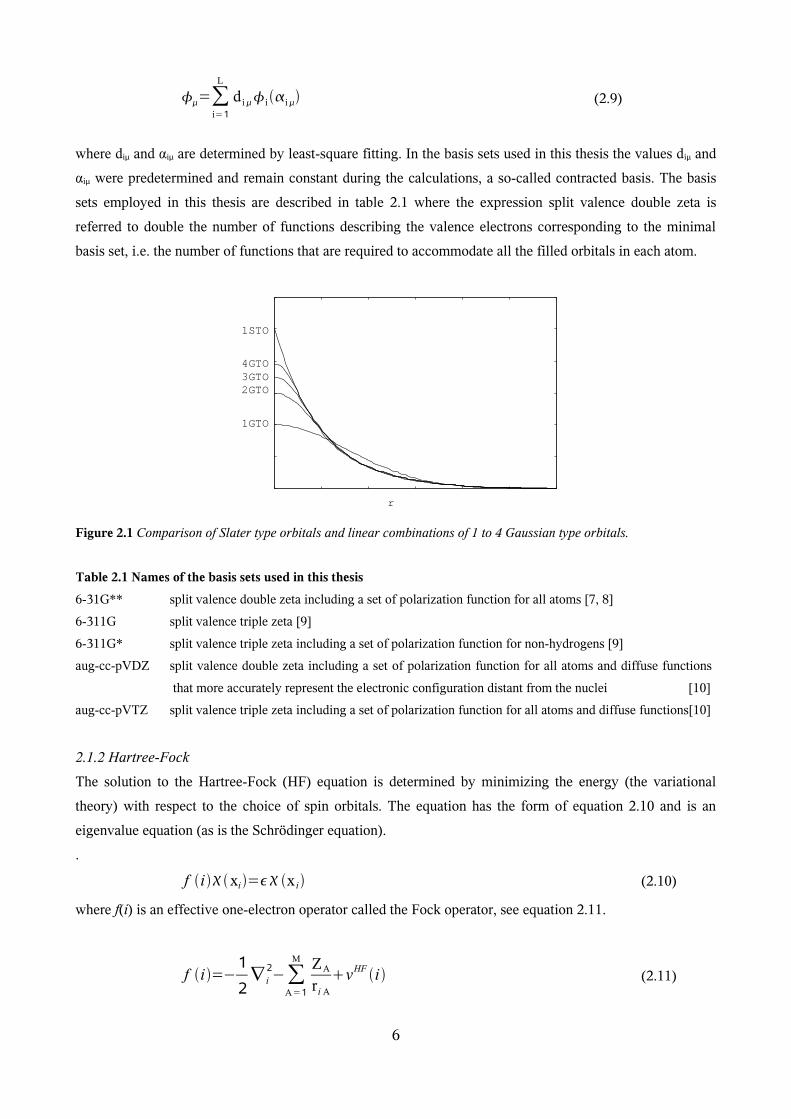
However, GTO:s do have disadvantages – for instance the STO:s do not have a cusp at the origin (see figure
2.1), i.e the values of the derivatives, at r=0, of the STO:s are negative while for the GTO:s it is zero. One
way to overcome the shortcomings of one GTO, is to express the basis sets as linear combinations of several
GTO:s, see equation 2.9, since the expansions improve the description of the atomic orbitals (see figure 2.1).
The more functions added, the better the description.
5
=∑i=1
L
d iii (2.9)
where diμ and αiμ are determined by least-square fitting. In the basis sets used in this thesis the values diμ and
αiμ were predetermined and remain constant during the calculations, a so-called contracted basis. The basis
sets employed in this thesis are described in table 2.1 where the expression split valence double zeta is
referred to double the number of functions describing the valence electrons corresponding to the minimal
basis set, i.e. the number of functions that are required to accommodate all the filled orbitals in each atom.
Figure 2.1 Comparison of Slater type orbitals and linear combinations of 1 to 4 Gaussian type orbitals.
Table 2.1 Names of the basis sets used in this thesis
6-31G** split valence double zeta including a set of polarization function for all atoms [7, 8]
6-311G split valence triple zeta [9]
6-311G* split valence triple zeta including a set of polarization function for non-hydrogens [9]
aug-cc-pVDZ split valence double zeta including a set of polarization function for all atoms and diffuse functions
that more accurately represent the electronic configuration distant from the nuclei [10]
aug-cc-pVTZ split valence triple zeta including a set of polarization function for all atoms and diffuse functions[10]
2.1.2 Hartree-Fock
The solution to the Hartree-Fock (HF) equation is determined by minimizing the energy (the variational
theory) with respect to the choice of spin orbitals. The equation has the form of equation 2.10 and is an
eigenvalue equation (as is the Schrödinger equation).
.
f ixi= x i (2.10)
where f(i) is an effective one-electron operator called the Fock operator, see equation 2.11.
f i=−1
2∇ i
2−∑A=1
M ZA
ri A
vHF i (2.11)
6
1STO
r
1GTO
2GTO3GTO4GTO
where vHF(i) is the average potential experienced by the ith electron due to the presence of the other
electrons. In order to simplify the Schrödinger equation, the many-body problem is approximated with an
one-electron problem in which the electron-electron repulsion is treated in an average way – the Hartree-
Fock Approximation. Since vHF(i) depends on the spin orbitals of the other electrons, the Hartree-Fock
equation is non-linear and must be solved iteratively. This procedure is called the self-consistent-field (SCF)
and the idea is to make an initial guess at the spin orbitals, calculate the average field (i.e. vHF(i)) and then
solve the Hartree-Fock equation. The spin orbitals obtained are subsequently used in order to calculate a new
field and a new set of spin orbitals. The procedure is repeated until self-consistency is reached.
The disadvantage with the HF method is that it fails to describe the electron correlation – the equation does
not take the correlation of the motion of the electrons into account. In other words the instantaneous
Coulomb interactions that keeps the electrons of opposite spin apart are not accounted for. Consequently the
energy from HF is too high - the difference between the HF energy and the exact energy is defined as the
correlation energy. However, it should be remembered that while HF already determines the total energy
99% correctly small energy differences are relevant in chemistry for instance in chemical reactions.
2.1.3 Many-body Perturbation Theory
One way of tackling the electron correlation is to split the total Hamiltonian, H, in two pieces: a zeroth-order
part, H0, which has known eigenfunctions and a perturbation, H' (see equation 2.12). When the zeroth order
Hamiltonian is the HF Hamiltonian, the many-body perturbation theory is referred to as MØller-Plesset
(MP).
H = H 0 +λ H' (2.12)
where λ is a parameter between 0 and 1 which describes the strength of the perturbation. The first, second,
etc order wave function can be described as a Taylor expansion in powers of the perturbation parameter, see
equation 2.13 and 2.14.
E=∑i=0
n
i E i (2.13)
=∑i=0
n
ii (2.14)
The higher the order of corrections, the more complicated types of equation need to be considered for the
energy correction. The second order corrections, MP2, accounts for about 80-90% of the electron correlation
and is the most economical wave function based method including electron correlation.
7
2.1.4 Coupled Cluster methods (CC)
Coupled Cluster theory is one of the more reliable QM methods but is also more computationally expensive
and was therefore only used as a reference in this thesis. The theory also uses the HF equation as a base but
the wave function is improved by adding a cluster function. The purpose of the functions is to correlate the
motions of any two electrons within a selected pair of occupied orbitals. The complexity of the equations and
the corresponding computer codes, as well as the cost of the computation increases sharply with the highest
level of excitation (the quantum state with the highest energy allowed). For many applications sufficient
accuracy may be obtained with the so-called CCSD, which includes single and double excitations, and the
more accurate (and more expensive) CCSD(T) is often called "the gold standard of quantum chemistry" for
its excellent compromise between the accuracy and the cost for the molecules near equilibrium geometries.
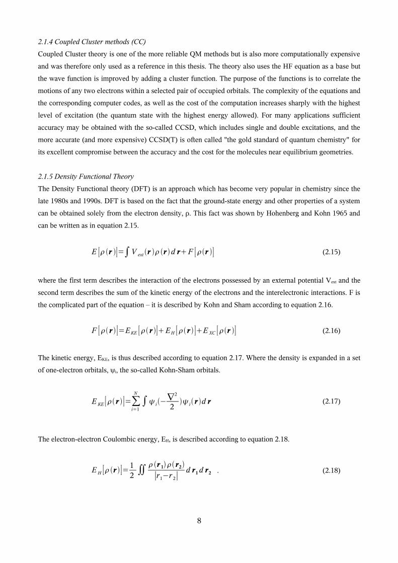
2.1.5 Density Functional Theory
The Density Functional theory (DFT) is an approach which has become very popular in chemistry since the
late 1980s and 1990s. DFT is based on the fact that the ground-state energy and other properties of a system
can be obtained solely from the electron density, ρ. This fact was shown by Hohenberg and Kohn 1965 and
can be written as in equation 2.15.
E 〚r 〛=∫V ext r r d rF 〚r 〛 (2.15)
where the first term describes the interaction of the electrons possessed by an external potential Vext and the
second term describes the sum of the kinetic energy of the electrons and the interelectronic interactions. F is
the complicated part of the equation – it is described by Kohn and Sham according to equation 2.16.
F 〚 r 〛=EKE 〚 r 〛EH 〚 r 〛E XC 〚r 〛 (2.16)
The kinetic energy, EKE, is thus described according to equation 2.17. Where the density is expanded in a set
of one-electron orbitals, ψi, the so-called Kohn-Sham orbitals.
E KE 〚 r 〛=∑i=1
N
∫i−∇2
2 i r d r (2.17)
The electron-electron Coulombic energy, EH, is described according to equation 2.18.
E H 〚r 〛=1 2 ∬ r 1 r2
∣r1−r 2 ∣d r1 d r2 . (2.18)
8
The Exc component is the crucial feature to the DFT theory, its exact form is not known, therefore it has been
expressed in very many alternative approximate ways. This thesis employed the BLYP expression, i.e.
Becke's (B) description for the exchange energy and Lee, Yang and Parr's definition for the correlation
energy.
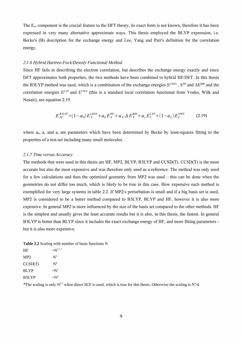
2.1.6 Hybrid Hartree-Fock/Density Functional Method
Since HF fails in describing the electron correlation, but describes the exchange energy exactly and since
DFT approximates both properties, the two methods have been combined to hybrid HF/DFT. In this thesis
the B3LYP method was used, which is a combination of the exchange energies ELSDA , EHF and ΔEB88 and the
correlation energies ELYP and EVWN (this is a standard local correlation functional from Vosko, Wilk and
Nusair), see equation 2.19.
E XCB3LYP=1−a0 E X
LSDAa0 E XHFa X E X
B88ac ECLYP1−aC EC
VWN (2.19)
where a0, ax and ac are parameters which have been determined by Becke by least-squares fitting to the
properties of a test-set including many small molecules.
2.1.7 Time versus Accuracy
The methods that were used in this thesis are HF, MP2, BLYP, B3LYP and CCSD(T). CCSD(T) is the most
accurate but also the most expensive and was therefore only used as a reference. The method was only used
for a few calculations and then the optimized geometry from MP2 was used – this can be done when the
geometries do not differ too much, which is likely to be true in this case. How expensive each method is
exemplified for very large systems in table 2.2. If MP2:s perturbation is small and if a big basis set is used,
MP2 is considered to be a better method compared to B3LYP, BLYP and HF, however it is also more
expensive. In general MP2 is more influenced by the size of the basis set compared to the other methods. HF
is the simplest and usually gives the least accurate results but it is also, in this thesis, the fastest. In general
B3LYP is better than BLYP since it includes the exact exchange energy of HF, and more fitting parameters -
but it is also more expensive.
Table 2.2 Scaling with number of basis functions N
HF ~N2.7 *
MP2 N5
CCSD(T) N8
BLYP ~N3
B3LYP ~N4
*The scaling is only N2.7 when direct SCF is used, which is true for this thesis. Otherwise the scaling is N4/4.
9
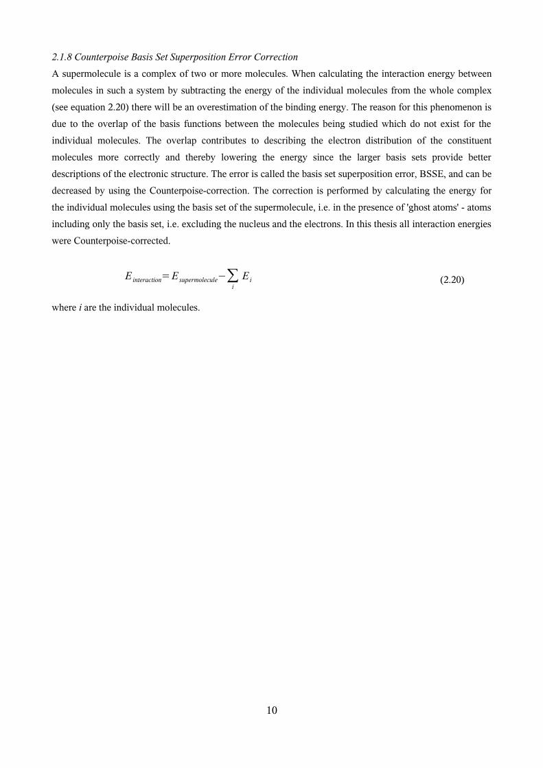
2.1.8 Counterpoise Basis Set Superposition Error Correction
A supermolecule is a complex of two or more molecules. When calculating the interaction energy between
molecules in such a system by subtracting the energy of the individual molecules from the whole complex
(see equation 2.20) there will be an overestimation of the binding energy. The reason for this phenomenon is
due to the overlap of the basis functions between the molecules being studied which do not exist for the
individual molecules. The overlap contributes to describing the electron distribution of the constituent
molecules more correctly and thereby lowering the energy since the larger basis sets provide better
descriptions of the electronic structure. The error is called the basis set superposition error, BSSE, and can be
decreased by using the Counterpoise-correction. The correction is performed by calculating the energy for
the individual molecules using the basis set of the supermolecule, i.e. in the presence of 'ghost atoms' - atoms
including only the basis set, i.e. excluding the nucleus and the electrons. In this thesis all interaction energies
were Counterpoise-corrected.
E interaction=E supermolecule−∑i
E i (2.20)
where i are the individual molecules.
10
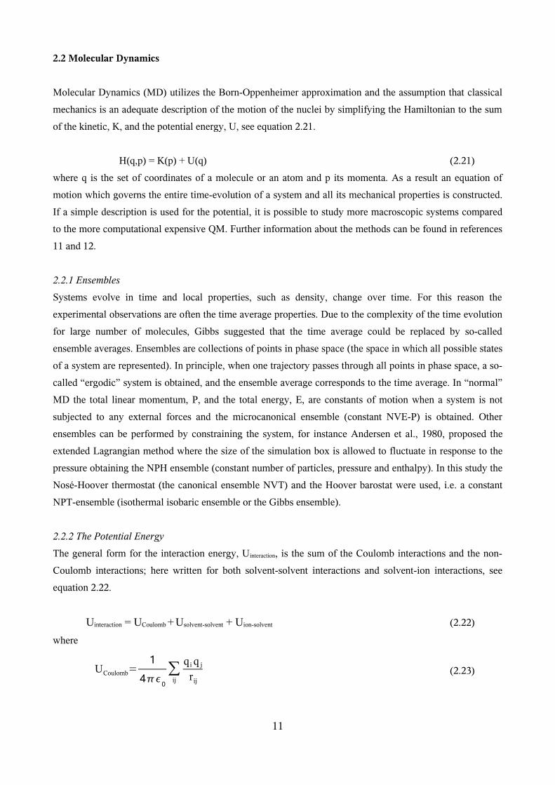
2.2 Molecular Dynamics
Molecular Dynamics (MD) utilizes the Born-Oppenheimer approximation and the assumption that classical
mechanics is an adequate description of the motion of the nuclei by simplifying the Hamiltonian to the sum
of the kinetic, K, and the potential energy, U, see equation 2.21.
H(q,p) = K(p) + U(q) (2.21)
where q is the set of coordinates of a molecule or an atom and p its momenta. As a result an equation of
motion which governs the entire time-evolution of a system and all its mechanical properties is constructed.
If a simple description is used for the potential, it is possible to study more macroscopic systems compared
to the more computational expensive QM. Further information about the methods can be found in references
11 and 12.
2.2.1 Ensembles
Systems evolve in time and local properties, such as density, change over time. For this reason the
experimental observations are often the time average properties. Due to the complexity of the time evolution
for large number of molecules, Gibbs suggested that the time average could be replaced by so-called
ensemble averages. Ensembles are collections of points in phase space (the space in which all possible states
of a system are represented). In principle, when one trajectory passes through all points in phase space, a so-
called “ergodic” system is obtained, and the ensemble average corresponds to the time average. In “normal”
MD the total linear momentum, P, and the total energy, E, are constants of motion when a system is not
subjected to any external forces and the microcanonical ensemble (constant NVE-P) is obtained. Other
ensembles can be performed by constraining the system, for instance Andersen et al., 1980, proposed the
extended Lagrangian method where the size of the simulation box is allowed to fluctuate in response to the
pressure obtaining the NPH ensemble (constant number of particles, pressure and enthalpy). In this study the
Nosé-Hoover thermostat (the canonical ensemble NVT) and the Hoover barostat were used, i.e. a constant
NPT-ensemble (isothermal isobaric ensemble or the Gibbs ensemble).
2.2.2 The Potential Energy
The general form for the interaction energy, Uinteraction, is the sum of the Coulomb interactions and the non-
Coulomb interactions; here written for both solvent-solvent interactions and solvent-ion interactions, see
equation 2.22.
Uinteraction = UCoulomb + Usolvent-solvent + Uion-solvent (2.22)
where
UCoulomb=1
40
∑ij
q i q j
rij(2.23)
11
Permanent dipoles occur when two or more atoms in a molecule have different electronegativity. An
example is water. The oxygen attracts the electrons more and thereby becomes more negative while the
hydrogens become more positive. A polar molecule is a molecule with a permanent dipole. An induced
dipole moment occurs when a polar molecule attracts the electrons of another atom or molecule. The solvent
model used in this thesis includes effects of induced dipole moments and is based on the “shell model”. The
shell model describes each ion or atom as a pair of point charges which include a positive “core” charge
located at the site of the nucleus and a negative “shell” charge; the charges are connected by a harmonic
spring, with the spring constant related to the polarisability. When a shell-model atom approaches a charged
ion or dipolar molecule, the potential energy is lowered by allowing the shell and the core to separate - an
induced dipole moment is produced.
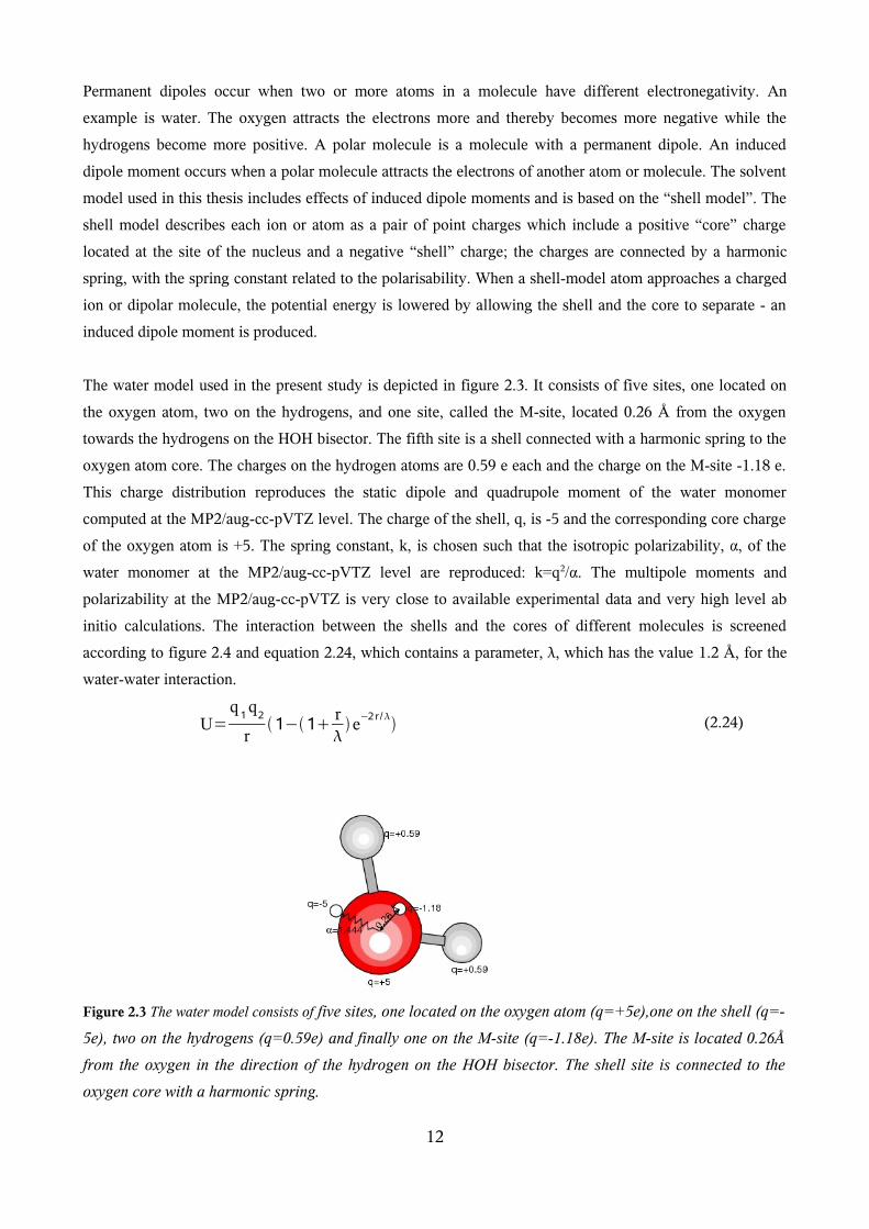
The water model used in the present study is depicted in figure 2.3. It consists of five sites, one located on
the oxygen atom, two on the hydrogens, and one site, called the M-site, located 0.26 Å from the oxygen
towards the hydrogens on the HOH bisector. The fifth site is a shell connected with a harmonic spring to the
oxygen atom core. The charges on the hydrogen atoms are 0.59 e each and the charge on the M-site -1.18 e.
This charge distribution reproduces the static dipole and quadrupole moment of the water monomer
computed at the MP2/aug-cc-pVTZ level. The charge of the shell, q, is -5 and the corresponding core charge
of the oxygen atom is +5. The spring constant, k, is chosen such that the isotropic polarizability, α, of the
water monomer at the MP2/aug-cc-pVTZ level are reproduced: k=q2/α. The multipole moments and
polarizability at the MP2/aug-cc-pVTZ is very close to available experimental data and very high level ab
initio calculations. The interaction between the shells and the cores of different molecules is screened
according to figure 2.4 and equation 2.24, which contains a parameter, λ, which has the value 1.2 Å, for the
water-water interaction.
U=q1q2
r1−1 r
e
−2 r / (2.24)
Figure 2.3 The water model consists of five sites, one located on the oxygen atom (q=+5e),one on the shell (q=-
5e), two on the hydrogens (q=0.59e) and finally one on the M-site (q=-1.18e). The M-site is located 0.26Å
from the oxygen in the direction of the hydrogen on the HOH bisector. The shell site is connected to the
oxygen core with a harmonic spring.
12
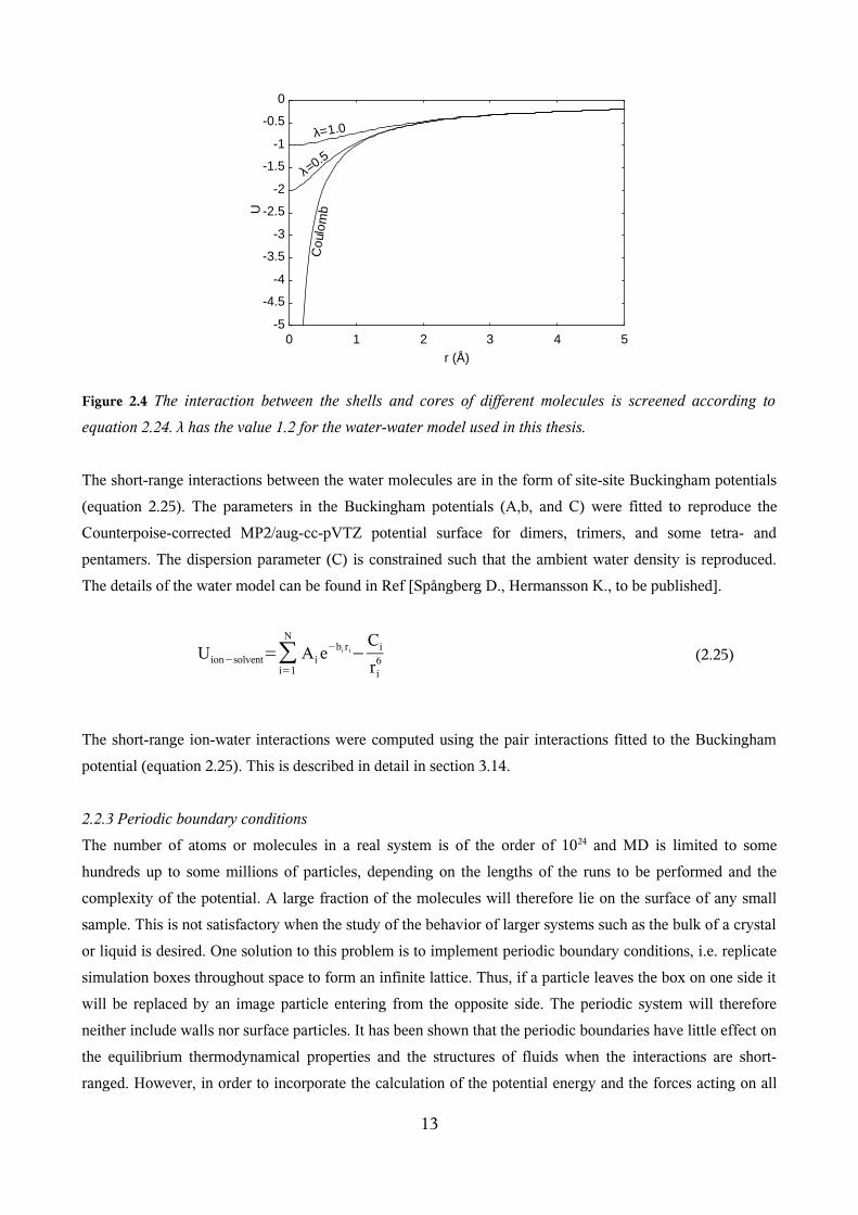
Figure 2.4 The interaction between the shells and cores of different molecules is screened according to
equation 2.24. λ has the value 1.2 for the water-water model used in this thesis.
The short-range interactions between the water molecules are in the form of site-site Buckingham potentials
(equation 2.25). The parameters in the Buckingham potentials (A,b, and C) were fitted to reproduce the
Counterpoise-corrected MP2/aug-cc-pVTZ potential surface for dimers, trimers, and some tetra- and
pentamers. The dispersion parameter (C) is constrained such that the ambient water density is reproduced.
The details of the water model can be found in Ref [Spångberg D., Hermansson K., to be published].
Uion−solvent=∑i=1
N
Ai e−bi r i−
Ci
ri6 (2.25)
The short-range ion-water interactions were computed using the pair interactions fitted to the Buckingham
potential (equation 2.25). This is described in detail in section 3.14.
2.2.3 Periodic boundary conditions
The number of atoms or molecules in a real system is of the order of 1024 and MD is limited to some
hundreds up to some millions of particles, depending on the lengths of the runs to be performed and the
complexity of the potential. A large fraction of the molecules will therefore lie on the surface of any small
sample. This is not satisfactory when the study of the behavior of larger systems such as the bulk of a crystal
or liquid is desired. One solution to this problem is to implement periodic boundary conditions, i.e. replicate
simulation boxes throughout space to form an infinite lattice. Thus, if a particle leaves the box on one side it
will be replaced by an image particle entering from the opposite side. The periodic system will therefore
neither include walls nor surface particles. It has been shown that the periodic boundaries have little effect on
the equilibrium thermodynamical properties and the structures of fluids when the interactions are short-
ranged. However, in order to incorporate the calculation of the potential energy and the forces acting on all
13
-5
-4.5
-4
-3.5
-3
-2.5
-2
-1.5
-1
-0.5
0
0 1 2 3 4 5
r (Å)
U
Cou
lom
b
λ=0.5
λ=1.0
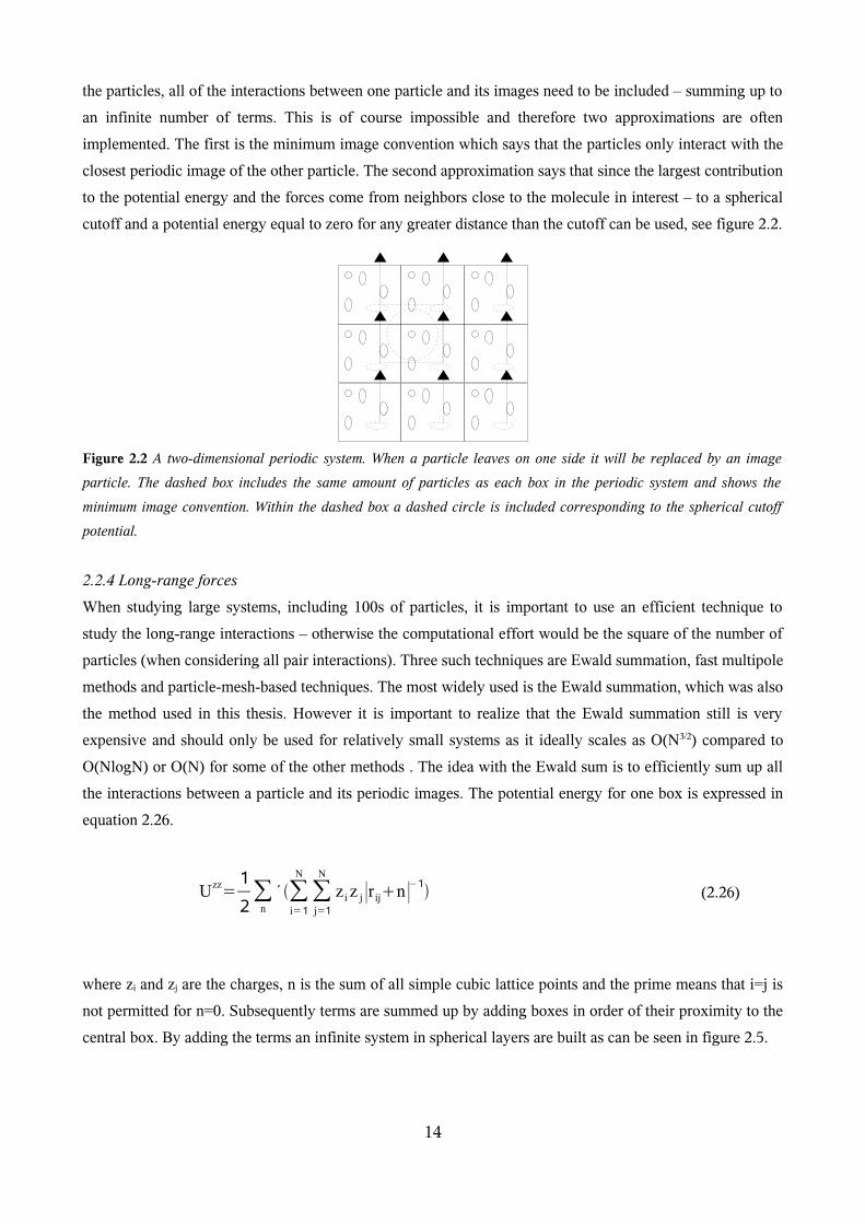
the particles, all of the interactions between one particle and its images need to be included – summing up to
an infinite number of terms. This is of course impossible and therefore two approximations are often
implemented. The first is the minimum image convention which says that the particles only interact with the
closest periodic image of the other particle. The second approximation says that since the largest contribution
to the potential energy and the forces come from neighbors close to the molecule in interest – to a spherical
cutoff and a potential energy equal to zero for any greater distance than the cutoff can be used, see figure 2.2.
Figure 2.2 A two-dimensional periodic system. When a particle leaves on one side it will be replaced by an image
particle. The dashed box includes the same amount of particles as each box in the periodic system and shows the
minimum image convention. Within the dashed box a dashed circle is included corresponding to the spherical cutoff
potential.
2.2.4 Long-range forces
When studying large systems, including 100s of particles, it is important to use an efficient technique to
study the long-range interactions – otherwise the computational effort would be the square of the number of
particles (when considering all pair interactions). Three such techniques are Ewald summation, fast multipole
methods and particle-mesh-based techniques. The most widely used is the Ewald summation, which was also
the method used in this thesis. However it is important to realize that the Ewald summation still is very
expensive and should only be used for relatively small systems as it ideally scales as O(N3/2) compared to
O(NlogN) or O(N) for some of the other methods . The idea with the Ewald sum is to efficiently sum up all
the interactions between a particle and its periodic images. The potential energy for one box is expressed in
equation 2.26.
Uzz=1
2∑
n
´ ∑i=1
N
∑j=1
N
z i z j ∣r ijn∣−1 (2.26)
where zi and zj are the charges, n is the sum of all simple cubic lattice points and the prime means that i=j is
not permitted for n=0. Subsequently terms are summed up by adding boxes in order of their proximity to the
central box. By adding the terms an infinite system in spherical layers are built as can be seen in figure 2.5.
14
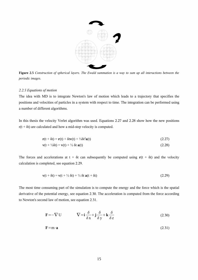
Figure 2.5 Construction of spherical layers. The Ewald summation is a way to sum up all interactions between the
periodic images.
2.2.5 Equations of motion
The idea with MD is to integrate Newton's law of motion which leads to a trajectory that specifies the
positions and velocities of particles in a system with respect to time. The integration can be performed using
a number of different algorithms.
In this thesis the velocity Verlet algorithm was used. Equations 2.27 and 2.28 show how the new positions
r(t + δt) are calculated and how a mid-step velocity is computed.
r(t + δt) = r(t) + δtv(t) + ½δt2a(t) (2.27)
v(t + ½δt) = v(t) + ½ δt a(t) (2.28)
The forces and accelerations at t + δt can subsequently be computed using r(t + δt) and the velocity
calculation is completed, see equation 2.29.
v(t + δt) = v(t + ½ δt) + ½ δt a(t + δt) (2.29)
The most time consuming part of the simulation is to compute the energy and the force which is the spatial
derivative of the potential energy, see equation 2.30. The acceleration is computed from the force according
to Newton's second law of motion, see equation 2.31.
F=−∇ U ∇=ix
j y
kz
(2.30)
F=m⋅a (2.31)
15

2.2.6 Constraint dynamics
In this thesis the molecules were considered to be rigid. One way of handling the dynamics of such a system
is the SHAKE approach [11] where the bond-lengths are constrained by solving the equations of motion for
one time-step in the absence of the constraint forces and subsequently their magnitudes are determined and
the atomic positions corrected. Since SHAKE was derived for the Verlet algorithm, a modification of
SHAKE called RATTLE was proposed by Andersen in 1983 for the velocity Verlet algorithm. The
difference is that the velocity Verlet algorithm includes two integration steps (see above) instead of one – in
RATTLE the first adjusts the atoms coordinates and velocity and at the second step the velocity along the
bonds are corrected.
16
3 Methods
The methods used in this study includes the optimization of potassium-water clusters, followed by the
computation of the interaction energy as a function of the ion-water distance. Subsequently, the potential
energies were fitted to the analytical potential functions which was used in the MD simulations and the
analyses of the simulation data.
3.1 Quantum Mechanical Calculations
3.1.1 Selection of Method and Basis Set
Before optimizing the geometry and before developing the potential energy curves for the clusters it is
important to chose appropriate methods and basis sets. Numerous methods and basis sets were evaluated by
performing calculations for one potassium ion and one water molecule. The methods included were HF,
MP2(FULL), BLYP and B3LYP, while CCSD(T)(FULL) was used as a reference. FULL is an option in
MP2 and CCSD(T) which signifies that all inner-core electrons are included in the correlation calculation.
This option was chosen since the frozen core otherwise includes all electrons of the K+, i.e. no perturbation
involving potassium would be included. The basis sets in table 2.1 were included for each method in the
evaluation. The methods and basis sets were selected by comparing the Counterpoise-corrected interaction
energies, Einteraction, and the optimized geometries with the results from the CCSD(T)(FULL) calculation and
results from the literature. The three best methods and the three best basis sets were used when optimizing
the remaining clusters.
The methods and basis sets were further evaluated by computing the interaction energy as a function of the
ion-water distance for the potassium ion and a single water molecule. The function was also computed using
the 6-311g*(K)aug-cc-pVQZ(H2O) and the 6-311g(2df)(K)aug-cc-pVTZ(H2O) basis set for each of the
methods. The functions were subsequently used as references. The best methods and basis sets were selected
for computing the interaction energy function for the remaining clusters. All quantum chemical calculations
were performed with the GAMESS/US program [13]
3.1.2 Optimization of [K(H2O)2-8]+
The geometries and the energies of the optimized clusters containing one K+ surrounded by 2-8 water
molecules were studied. The purpose of this part of the work was to find the optimal geometry for the first
solvation shell structures incorporating different coordination numbers. It is known that in the gas phase the
water-water interaction is energetically favored compared to the ion-water interactions for K+(H2O)n systems
with large n [14], leading to a global minimum with low K+ -H2O coordination numbers. However, since the
goal of this thesis was to study potassium in bulk water and not in the gas phase and since potassium has a
larger coordination number in bulk water than in the gas phase, only clusters with rather high K+ -H2O
coordination numbers were considered. The initial cluster configuration were chosen so that all water
molecules pointed towards the potassium ion and had approximately the same ion-oxygen distance.
17
3.1.2 The Potential Energy Curve
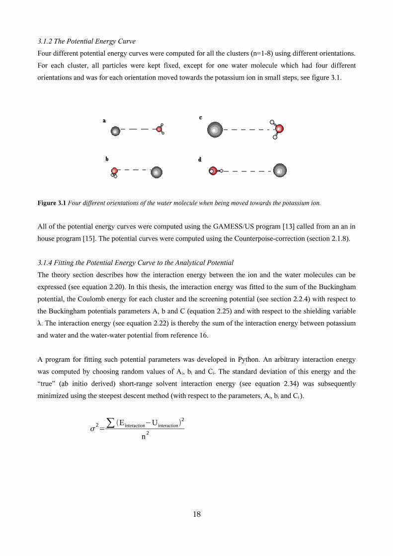
Four different potential energy curves were computed for all the clusters (n=1-8) using different orientations.
For each cluster, all particles were kept fixed, except for one water molecule which had four different
orientations and was for each orientation moved towards the potassium ion in small steps, see figure 3.1.
Figure 3.1 Four different orientations of the water molecule when being moved towards the potassium ion.
All of the potential energy curves were computed using the GAMESS/US program [13] called from an an in
house program [15]. The potential curves were computed using the Counterpoise-correction (section 2.1.8).
3.1.4 Fitting the Potential Energy Curve to the Analytical Potential
The theory section describes how the interaction energy between the ion and the water molecules can be
expressed (see equation 2.20). In this thesis, the interaction energy was fitted to the sum of the Buckingham
potential, the Coulomb energy for each cluster and the screening potential (see section 2.2.4) with respect to
the Buckingham potentials parameters A, b and C (equation 2.25) and with respect to the shielding variable
λ. The interaction energy (see equation 2.22) is thereby the sum of the interaction energy between potassium
and water and the water-water potential from reference 16.
A program for fitting such potential parameters was developed in Python. An arbitrary interaction energy
was computed by choosing random values of Ai, bi and Ci. The standard deviation of this energy and the
“true” (ab initio derived) short-range solvent interaction energy (see equation 2.34) was subsequently
minimized using the steepest descent method (with respect to the parameters, Ai, bi and Ci ).
2=∑ E interaction−Uinteraction2
n2
18
3.2 Molecular Dynamics
3.2.1 Simulation Protocol
The molecular-dynamics simulations were performed for liquid systems, including 1024 water molecules
and a single ion. The simulation used cubic periodic boundary conditions, with spherical cutoffs at 13 Å,
which were employed for short-range interactions, and Ewald lattice sums [12] were used for the Coulomb
interactions. The simulation time step was 0.5 fs, the velocity Verlet integrator [12] was employed in order to
integrate the equations of motion and the RATTLE method was used to keep the molecules rigid. Finally, the
method of Nosé and Hoover [12] and the method of Hoover [12] were applied to obtain the NPT ensemble,
with parameters set to keep ambient conditions of an average temperature of 300K and an average pressure
of 0 Pa.
The initial configurations need to be designed in such a way that it can relax quickly to the structure and
velocity distribution appropriate of a fluid. The water molecules and the potassium ion were placed randomly
on a primitive lattice in a volume corresponding to a density of 0.06g/cm3. For 1000 time steps the
coordinates and velocities were integrated and the density slightly increased at each time step – this was done
until the density reached 1g/cm3. The system was thereafter simulated for another 1000 time steps at a fixed
density of 1g/cm3. During these two procedures the velocities of the particles were scaled to correspond a
temperature of 300K. The following step, the run to reach equilibration, was performed in 5000 time steps
while the volume of the cell was smoothly changed to correspond to a pressure of 0 Pa using the Berendsen
weak coupling sheme [12]. In the last step, the procedure run, the system was simulated for 1 500 000 time
steps, corresponding to 750 ps of the simulation time. More detailed information about the simulation
protocol can be found in reference 17.
3.2.2 Analysis of Molecular Dynamic Simulation Results
The aim of this thesis was to study the structure of potassium in water, i.e. properties such as the
coordination number and the coordination geometry. Functions such as the radial distribution, the angular
distribution and the spatial distribution function were used in order to visualize these properties.
The Coordination Number
The radial distribution function is the collective name for pair, triplet or higher radial functions. The pair
distribution function, g(r), gives the probability of finding a pair of particles at a distance, r, apart, relative to
the probability expected in an ideal gas distribution of the same overall density. In other words it
characterizes the local structure of a fluid by describing how many particles β surround particle α, see
equation 3.1.
g−=n r
V r (3.1)
19
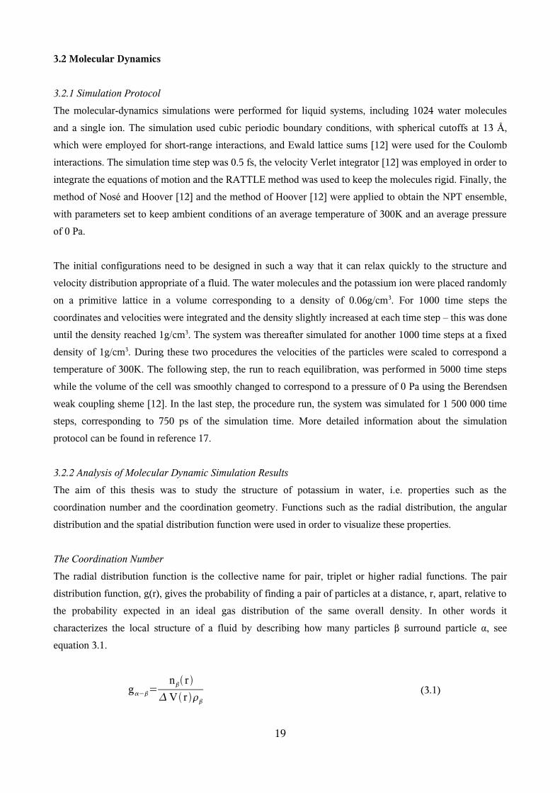
where nβ is the number of β particles in a thin spherical shell between r and r+Δr from an α particle, see
figure 3.2. ρβ is the number density of β-particles (total number of β-particles/total volume) and ΔV(r) is the
volume of the thin spherical shell.
Figure 3.2 A sphere where an α – particle is placed in the center and where nβ is the number of β particles within the
shell between r and r+Δr.
By integrating the radial distribution function, the number of particles surrounding the α particle is obtained,
see equation 3.2. The coordination number is most often and in this thesis defined as the number of particles
surrounding the α particle between 0 and the distance where g(r) has its first minimum. See also references 5
and 11.
n− r =∫0
r
g− r V r dr (3.2)
The coordination of the potassium ion was also studied by looking at the distribution of the coordination
numbers, i.e. a histogram constructed to show how high probability a certain coordination number has.
The Orientation of the Water Molecules
The orientation of the water molecules was studied by looking at tilt angles, see figure 3.3. Angles
substantially smaller than 180o are classified as “tetrahedral” while angles close to 180o as “trigonal”. The
characteristics of bulk water is the typical tetrahedral orientation, suggesting that the water molecules that are
surrounding the ions in the first solvation shell, accept hydrogen bonds from the second solvation shell. In
this thesis the angle distribution was computed for the first solvation shell using two different definitions
with two variations of the first definition following reference 18. The first was defined as θdip and is the angle
between the oxygen-ion vector and the water bisector, see figure 3.3. Two distributions, one of the θdip itself
and one of the cosine of the θdip were computed. The second tilt angle was defined as θdihed and is the angle
between the plane of the water molecule and the plane containing the ion and and two hydrogen atoms which
have been translated in the water plane so that the midpoint of the two hydrogens corresponds to the
untranslated oxygen, see figure 3.4. The translation is done to ensure that all angles are equal for the different
definitions in the special case when the two ion-hydrogen distances are the same.
20
r
Δr
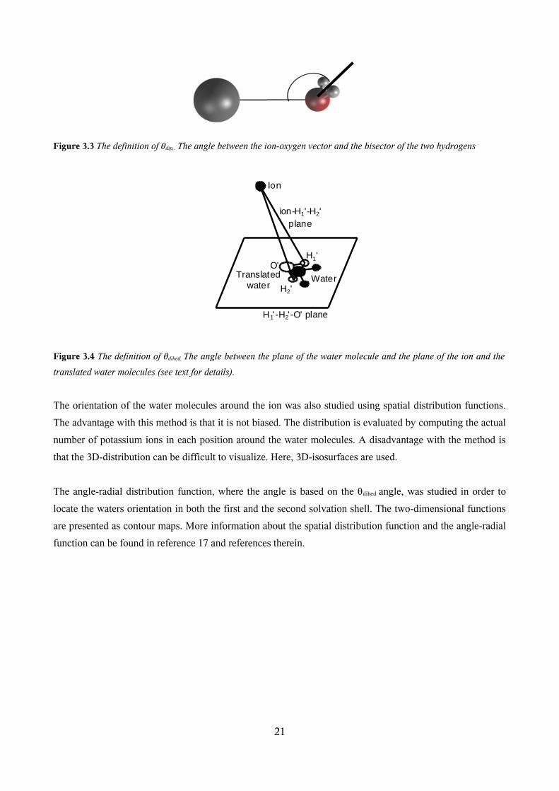
Figure 3.3 The definition of θdip,. The angle between the ion-oxygen vector and the bisector of the two hydrogens
Figure 3.4 The definition of θdihed. The angle between the plane of the water molecule and the plane of the ion and the
translated water molecules (see text for details).
The orientation of the water molecules around the ion was also studied using spatial distribution functions.
The advantage with this method is that it is not biased. The distribution is evaluated by computing the actual
number of potassium ions in each position around the water molecules. A disadvantage with the method is
that the 3D-distribution can be difficult to visualize. Here, 3D-isosurfaces are used.
The angle-radial distribution function, where the angle is based on the θdihed angle, was studied in order to
locate the waters orientation in both the first and the second solvation shell. The two-dimensional functions
are presented as contour maps. More information about the spatial distribution function and the angle-radial
function can be found in reference 17 and references therein.
21
Ion
WaterTranslatedwater
ion-H1'-H2'plane
H1' -H2' -O' plane
O'H1'
H2'
4 Results and Discussion
4.1 Quantum Mechanics
4.1.1 Selection of Methods and Basis Sets
Geometry optimization of the K+ ion and a single water molecule was performed for the different methods
and basis sets to determine the level needed to properly describe the K+-water interaction. The minimum
interaction energy and the corresponding distances between the oxygen and the potassium ion (for each of
the methods HF, MP2(FULL), BLYP and B3LYP) are presented in figures 4.1-4.4 and table 4.1. Numerous
theoretical studies that have been performed on water clusters and ion-water clusters show that the polarized
basis sets are necessary [14, 17-19]. It is also known that the additional shell of diffuse functions, that are
incorporated in the aug-cc-pVDZ and aug-cc-pVTZ basis sets, are important when describing the electric
moments and the polarizability of water and that they play an important role for the larger clusters where
water-water predominate [14]. Consequently, in the results only the basis sets including polarization
functions, 6-31g**, aug-cc-pVDZ and aug-cc-pVTZ, for water are presented.
For K+ the basis sets 6-311g, 6-31g* and 6-311g** were evaluated. For all the methods, except HF, the
obtained interaction energies were smaller for the basis sets that did not include polarization functions than
for the basis set that did include the functions. From the results it was therefore obvious that basis sets
including the polarization functions for potassium were necessary. This can partly be explained by the ion
being highly polarizable (due to its relatively large size) and that the interaction energy depends on the
induced dipole moment. The basis sets were further evaluated by computing the polarizabilities for the K+-
ion for all the methods and basis sets. The polarizability was also computed for the 6-311g(2df) basis set,
which includes a larger set of polarization functions, and was used as a reference. Table 4.2 shows that the
values of the 6-311g* basis set were very close to the reference. The corresponding polarizabilities of 6-31g*
were relatively close while the polarizabilities for the 6-311g basis set were much lower. The geometry
optimizations for the remaining clusters (n=2-8) were therefore performed only using the polarized basis sets
6-31g*, 6-311g*(K)aug-cc-pVDZ (H2O) and 6-311g* (K)aug-cc-pVTZ (H2O).
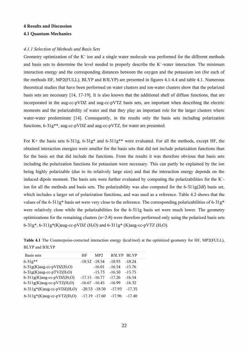
Table 4.1 The Counterpoise-corrected interaction energy (kcal/mol) at the optimized geometry for HF, MP2(FULL),
BLYP and B3LYP
Basis sets HF MP2 B3LYP BLYP
6-31g** -18.52 -18.54 -18.93 -18.246-31g(K)aug-cc-pVDZ(H2O) -16.01 -16.54 -15.766-31g(K)aug-cc-pTVZ(H2O) -15.73 -16.50 -15.756-311g(K)aug-cc-pVDZ(H2O) -17.15 -16.77 -17.26 -16.546-311g(K)aug-cc-pVTZ(H2O) -16.67 -16.45 -16.99 -16.32
6-311g*(K)aug-cc-pVDZ(H2O) -20.53 -18.50 -17.93 -17.35
6-311g*(K)aug-cc-pVTZ(H2O) -17.19 -17.60 -17.96 -17.40
22
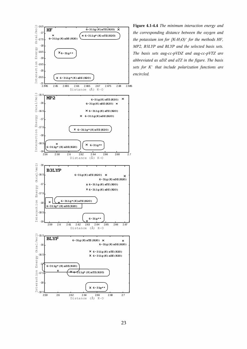
Figure 4.1-4.4 The minimum interaction energy and
the corresponding distance between the oxygen and
the potassium ion for [K-H2O)+ for the methods HF,
MP2, B3LYP and BLYP and the selected basis sets.
The basis sets aug-cc-pVDZ and aug-cc-pVTZ are
abbreviated as aDZ and aTZ in the figure. The basis
sets for K+ that include polarization functions are
encircled.
23
-19
-18.5
-18
-17.5
-17
-16.5
-16
-15.5
2.56 2.58 2.6 2.62 2.64 2.66 2.68 2.7
Interaction
Energy
(kcal/mol)
Distance (Å) K-O
6-311g*(K)aDZ(H2O)6-31g**
6-311g*(K)aTZ(H2O)
6-311g(K)aDZ(H2O)
6-311g(K)aTZ(H2O)
6-31g(K)aDZ(H2O)6-31g(K)aTZ(H2O)
-21
-20.5
-20
-19.5
-19
-18.5
-18
-17.5
-17
-16.5
2.645 2.65 2.655 2.66 2.665 2.67 2.675 2.68 2.685
Interaction
Energy
(kcal/mol)
Distance (Å) K-O
6-31g**
6-311g(K)aDZ(H2O)
6-311g(K)aTZ(H2O)
6-311g*(K)aTZ(H2O)
6-311g*(K)aDZ(H2O)
HF
MP2
-19
-18.5
-18
-17.5
-17
-16.5
-16
2.59 2.6 2.61 2.62 2.63 2.64 2.65 2.66 2.67
Interaction
Energy
(kcal/mol)
Distance (Å) K-O
-18.5
-18
-17.5
-17
-16.5
-16
-15.5
2.58 2.6 2.62 2.64 2.66 2.68 2.7
Interaction
Energy
(kcal/mol)
Distance (Å) K-O
6-31g**
6-311g*(K)aDZ(H2O)
6-311g*(K)aTZ(H2O)
6-311g(K)aDZ(H2O)6-311g(K)aTZ(H2O)
6-31g(K)aDZ(H2O)6-31g(K)aTZ(H2O)BLYP
B3LYP
6-31g**
6-311g*(K)aDZ(H2O)
6-311g*(K)aTZ(H2O)
6-311g(K)aDZ(H2O)
6-311g(K)aTZ(H2O)
6-31g(K)aTZ(H2O)
6-31g(K)aDZ(H2O)
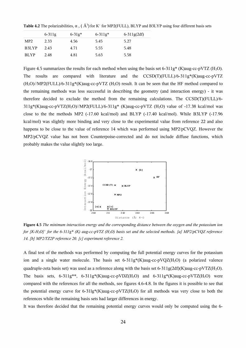
Table 4.2 The polarizabilities, α , ( Å3) for K+ for MP2(FULL), BLYP and B3LYP using four different basis sets
6-311g 6-31g* 6-311g* 6-311g(2df)
MP2 2.33 4.56 5.45 5.27
B3LYP 2.43 4.71 5.55 5.48
BLYP 2.48 4.81 5.63 5.58
Figure 4.5 summarizes the results for each method when using the basis set 6-311g* (K)aug-cc-pVTZ (H2O).
The results are compared with literature and the CCSD(T)(FULL)/6-311g*(K)aug-cc-pVTZ
(H2O)//MP2(FULL)/6-311g*(K)aug-cc-pVTZ (H2O) result. It can be seen that the HF method compared to
the remaining methods was less successful in describing the geometry (and interaction energy) - it was
therefore decided to exclude the method from the remaining calculations. The CCSD(T)(FULL)/6-
311g*(K)aug-cc-pVTZ(H2O)//MP2(FULL)/6-311g* (K)aug-cc-pVTZ (H2O) value of -17.38 kcal/mol was
close to the the methods MP2 (-17.60 kcal/mol) and BLYP (-17.40 kcal/mol). While B3LYP (-17.96
kcal/mol) was slightly more binding and very close to the experimental value from reference 22 and also
happens to be close to the value of reference 14 which was performed using MP2/pCVQZ. However the
MP2/pCVQZ value has not been Counterpoise-corrected and do not include diffuse functions, which
probably makes the value slightly too large.
Figure 4.5 The minimum interaction energy and the corresponding distance between the oxygen and the potassium ion
for [K-H2O]+ for the 6-311g* (K) aug-cc-pVTZ (H2O) basis set and the selected methods. [a] MP2/pCVQZ reference
14. [b] MP2/TZ2P reference 20. [c] experiment reference 2.
A final test of the methods was performed by computing the full potential energy curves for the potassium
ion and a single water molecule. The basis set 6-311g*(K)aug-cc-pVQZ(H2O) (a polarized valence
quadruple-zeta basis set) was used as a reference along with the basis set 6-311g(2df)(K)aug-cc-pVTZ(H2O).
The basis sets, 6-311g**, 6-311g*(K)aug-cc-pVDZ(H2O) and 6-311g*(K)aug-cc-pVTZ(H2O) were
compared with the references for all the methods, see figures 4.6-4.8. In the figures it is possible to see that
the potential energy curve for 6-31lg*(K)aug-cc-pVTZ(H2O) for all methods was very close to both the
references while the remaining basis sets had larger differences in energy.
It was therefore decided that the remaining potential energy curves would only be computed using the 6-
24
-18
-17.8
-17.6
-17.4
-17.2
-17
-16.8
2.58 2.6 2.62 2.64 2.66 2.68
Interaction
Energy
(kcal/mol)
Distance (Å) K-O
B3LYP[c][a]
MP2
BLYPCCSD(T)
[b]
HF
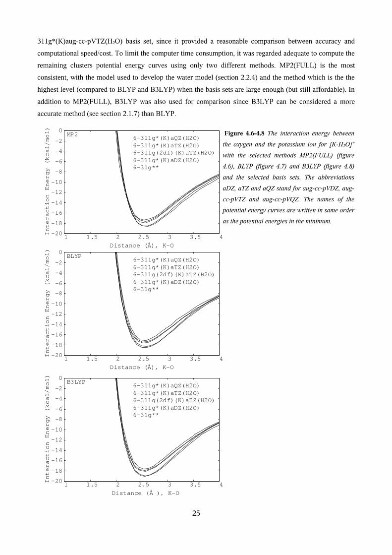
311g*(K)aug-cc-pVTZ(H2O) basis set, since it provided a reasonable comparison between accuracy and
computational speed/cost. To limit the computer time consumption, it was regarded adequate to compute the
remaining clusters potential energy curves using only two different methods. MP2(FULL) is the most
consistent, with the model used to develop the water model (section 2.2.4) and the method which is the the
highest level (compared to BLYP and B3LYP) when the basis sets are large enough (but still affordable). In
addition to MP2(FULL), B3LYP was also used for comparison since B3LYP can be considered a more
accurate method (see section 2.1.7) than BLYP.
Figure 4.6-4.8 The interaction energy between
the oxygen and the potassium ion for [K-H2O]+
with the selected methods MP2(FULL) (figure
4.6), BLYP (figure 4.7) and B3LYP (figure 4.8)
and the selected basis sets. The abbreviations
aDZ, aTZ and aQZ stand for aug-cc-pVDZ, aug-
cc-pVTZ and aug-cc-pVQZ. The names of the
potential energy curves are written in same order
as the potential energies in the minimum.
25
-20
-18
-16
-14
-12
-10
-8
-6
-4
-2
0
1 1.5 2 2.5 3 3.5 4Interaction
Energy
(kcal/mol)
Distance (Å), K-O
6-311g*(K)aQZ(H2O)6-311g*(K)aTZ(H2O)6-311g(2df)(K)aTZ(H2O)6-311g*(K)aDZ(H2O)6-31g**
MP2
-20
-18
-16
-14
-12
-10
-8
-6
-4
-2
0
1 1.5 2 2.5 3 3.5 4Interaction
Energy
(kcal/mol)
Distance (Å), K-O
6-311g*(K)aQZ(H2O)6-311g*(K)aTZ(H2O)6-311g(2df)(K)aTZ(H2O)6-311g*(K)aDZ(H2O)6-31g**
BLYP
-20
-18
-16
-14
-12
-10
-8
-6
-4
-2
0
1 1.5 2 2.5 3 3.5 4Interaction
Energy
(kcal/mol)
Distance (Å ), K-O
6-311g*(K)aTZ(H2O)
6-311g*(K)aDZ(H2O)6-31g**
6-311g*(K)aQZ(H2O)B3LYP
6-311g(2df)(K)aTZ(H2O)
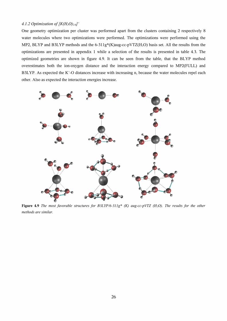
4.1.2 Optimization of [K(H2O)2-8]+
One geometry optimization per cluster was performed apart from the clusters containing 2 respectively 8
water molecules where two optimizations were performed. The optimizations were performed using the
MP2, BLYP and B3LYP methods and the 6-311g*(K)aug-cc-pVTZ(H2O) basis set. All the results from the
optimizations are presented in appendix 1 while a selection of the results is presented in table 4.3. The
optimized geometries are shown in figure 4.9. It can be seen from the table, that the BLYP method
overestimates both the ion-oxygen distance and the interaction energy compared to MP2(FULL) and
B3LYP. As expected the K+-O distances increase with increasing n, because the water molecules repel each
other. Also as expected the interaction energies increase.
Figure 4.9 The most favorable structures for B3LYP/6-311g* (K) aug-cc-pVTZ (H2O). The results for the other
methods are similar.
26
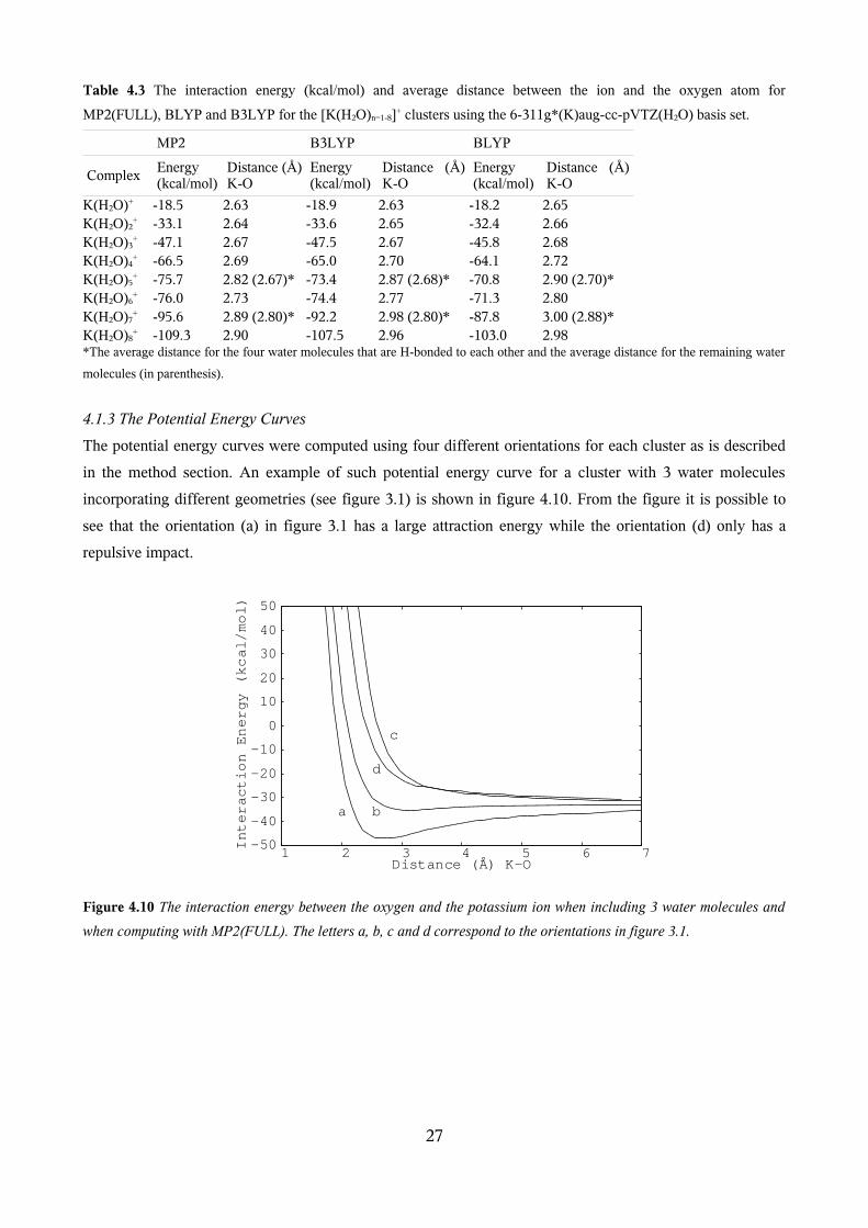
Table 4.3 The interaction energy (kcal/mol) and average distance between the ion and the oxygen atom for
MP2(FULL), BLYP and B3LYP for the [K(H2O)n=1-8]+ clusters using the 6-311g*(K)aug-cc-pVTZ(H2O) basis set.
MP2 B3LYP BLYP
ComplexEnergy (kcal/mol)
Distance (Å) K-O
Energy (kcal/mol)
Distance (Å) K-O
Energy (kcal/mol)
Distance (Å) K-O
K(H2O)+ -18.5 2.63 -18.9 2.63 -18.2 2.65K(H2O)2
+ -33.1 2.64 -33.6 2.65 -32.4 2.66K(H2O)3
+ -47.1 2.67 -47.5 2.67 -45.8 2.68K(H2O)4
+ -66.5 2.69 -65.0 2.70 -64.1 2.72K(H2O)5
+ -75.7 2.82 (2.67)* -73.4 2.87 (2.68)* -70.8 2.90 (2.70)*K(H2O)6
+ -76.0 2.73 -74.4 2.77 -71.3 2.80K(H2O)7
+ -95.6 2.89 (2.80)* -92.2 2.98 (2.80)* -87.8 3.00 (2.88)*K(H2O)8
+ -109.3 2.90 -107.5 2.96 -103.0 2.98*The average distance for the four water molecules that are H-bonded to each other and the average distance for the remaining water
molecules (in parenthesis).
4.1.3 The Potential Energy Curves
The potential energy curves were computed using four different orientations for each cluster as is described
in the method section. An example of such potential energy curve for a cluster with 3 water molecules
incorporating different geometries (see figure 3.1) is shown in figure 4.10. From the figure it is possible to
see that the orientation (a) in figure 3.1 has a large attraction energy while the orientation (d) only has a
repulsive impact.
Figure 4.10 The interaction energy between the oxygen and the potassium ion when including 3 water molecules and
when computing with MP2(FULL). The letters a, b, c and d correspond to the orientations in figure 3.1.
27
-50
-40
-30
-20
-10
0
10
20
30
40
50
1 2 3 4 5 6 7InteractionEnergy
(kcal/mol)
Distance (Å) K-O
a b
c
d
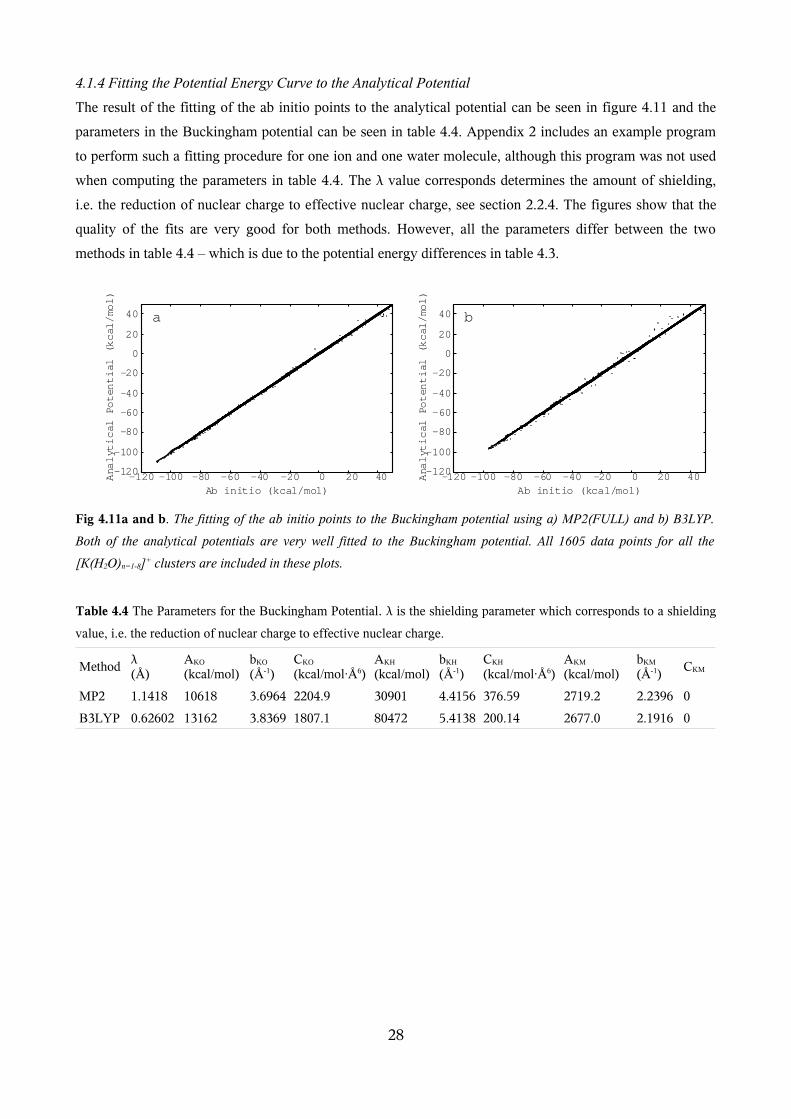
4.1.4 Fitting the Potential Energy Curve to the Analytical Potential
The result of the fitting of the ab initio points to the analytical potential can be seen in figure 4.11 and the
parameters in the Buckingham potential can be seen in table 4.4. Appendix 2 includes an example program
to perform such a fitting procedure for one ion and one water molecule, although this program was not used
when computing the parameters in table 4.4. The λ value corresponds determines the amount of shielding,
i.e. the reduction of nuclear charge to effective nuclear charge, see section 2.2.4. The figures show that the
quality of the fits are very good for both methods. However, all the parameters differ between the two
methods in table 4.4 – which is due to the potential energy differences in table 4.3.
Fig 4.11a and b. The fitting of the ab initio points to the Buckingham potential using a) MP2(FULL) and b) B3LYP.
Both of the analytical potentials are very well fitted to the Buckingham potential. All 1605 data points for all the
[K(H2O)n=1-8]+ clusters are included in these plots.
Table 4.4 The Parameters for the Buckingham Potential. λ is the shielding parameter which corresponds to a shielding
value, i.e. the reduction of nuclear charge to effective nuclear charge.
Method λ (Å)
AKO
(kcal/mol)bKO
(Å-1)CKO
(kcal/mol∙Å6)AKH
(kcal/mol)bKH
(Å-1)CKH
(kcal/mol∙Å6)AKM
(kcal/mol)bKM
(Å-1)CKM
MP2 1.1418 10618 3.6964 2204.9 30901 4.4156 376.59 2719.2 2.2396 0
B3LYP 0.62602 13162 3.8369 1807.1 80472 5.4138 200.14 2677.0 2.1916 0
28
-120
-100
-80
-60
-40
-20
0
20
40
-120 -100 -80 -60 -40 -20 0 20 40Analytical
Potential
(kcal/mol)
Ab initio (kcal/mol)
-120
-100
-80
-60
-40
-20
0
20
40
-120 -100 -80 -60 -40 -20 0 20 40Analytical
Potential
(kcal/mol)
Ab initio (kcal/mol)
a b
4.2 Molecular Dynamics
The Coordination Number
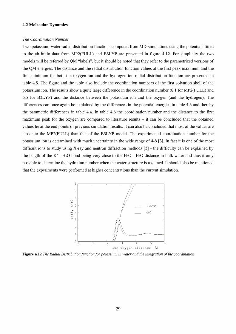
Two potassium-water radial distribution functions computed from MD-simulations using the potentials fitted
to the ab initio data from MP2(FULL) and B3LYP are presented in figure 4.12. For simplicity the two
models will be referred by QM “labels”, but it should be noted that they refer to the parametrized versions of
the QM energies. The distance and the radial distribution function values at the first peak maximum and the
first minimum for both the oxygen-ion and the hydrogen-ion radial distribution function are presented in
table 4.5. The figure and the table also include the coordination numbers of the first solvation shell of the
potassium ion. The results show a quite large difference in the coordination number (8.1 for MP2(FULL) and
6.5 for B3LYP) and the distance between the potassium ion and the oxygen (and the hydrogen). The
differences can once again be explained by the differences in the potential energies in table 4.3 and thereby
the parametric differences in table 4.4. In table 4.6 the coordination number and the distance to the first
maximum peak for the oxygen are compared to literature results – it can be concluded that the obtained
values lie at the end points of previous simulation results. It can also be concluded that most of the values are
closer to the MP2(FULL) than that of the B3LYP model. The experimental coordination number for the
potassium ion is determined with much uncertainty in the wide range of 4-8 [3]. In fact it is one of the most
difficult ions to study using X-ray and neutron diffraction methods [3] - the difficulty can be explained by
the length of the K+ - H2O bond being very close to the H2O - H2O distance in bulk water and thus it only
possible to determine the hydration number when the water structure is assumed. It should also be mentioned
that the experiments were performed at higher concentrations than the current simulation.
Figure 4.12 The Radial Distribution function for potassium in water and the integration of the coordination
29
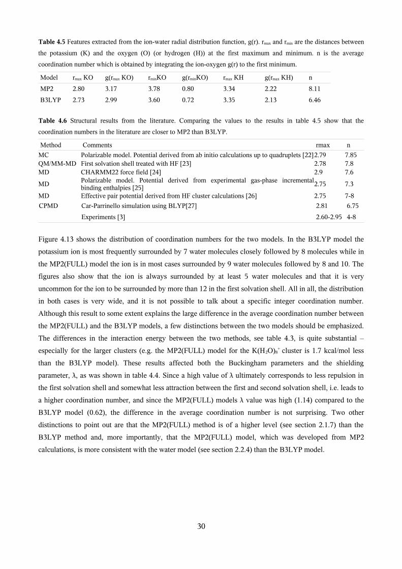
Table 4.5 Features extracted from the ion-water radial distribution function, g(r). rmax and rmin are the distances between
the potassium (K) and the oxygen (O) (or hydrogen (H)) at the first maximum and minimum. n is the average
coordination number which is obtained by integrating the ion-oxygen g(r) to the first minimum.
Model rmax KO g(rmax KO) rminKO g(rminKO) rmax KH g(rmax KH) n
MP2 2.80 3.17 3.78 0.80 3.34 2.22 8.11
B3LYP 2.73 2.99 3.60 0.72 3.35 2.13 6.46
Table 4.6 Structural results from the literature. Comparing the values to the results in table 4.5 show that the
coordination numbers in the literature are closer to MP2 than B3LYP.
Method Comments rmax n
MC Polarizable model. Potential derived from ab initio calculations up to quadruplets [22]2.79 7.85QM/MM-MD First solvation shell treated with HF [23] 2.78 7.8MD CHARMM22 force field [24] 2.9 7.6
MD Polarizable model. Potential derived from experimental gas-phase incremental binding enthalpies [25]
2.75 7.3
MD Effective pair potential derived from HF cluster calculations [26] 2.75 7-8
CPMD Car-Parrinello simulation using BLYP[27] 2.81 6.75
Experiments [3] 2.60-2.95 4-8
Figure 4.13 shows the distribution of coordination numbers for the two models. In the B3LYP model the
potassium ion is most frequently surrounded by 7 water molecules closely followed by 8 molecules while in
the MP2(FULL) model the ion is in most cases surrounded by 9 water molecules followed by 8 and 10. The
figures also show that the ion is always surrounded by at least 5 water molecules and that it is very
uncommon for the ion to be surrounded by more than 12 in the first solvation shell. All in all, the distribution
in both cases is very wide, and it is not possible to talk about a specific integer coordination number.
Although this result to some extent explains the large difference in the average coordination number between
the MP2(FULL) and the B3LYP models, a few distinctions between the two models should be emphasized.
The differences in the interaction energy between the two methods, see table 4.3, is quite substantial –
especially for the larger clusters (e.g. the MP2(FULL) model for the K(H2O)8+ cluster is 1.7 kcal/mol less
than the B3LYP model). These results affected both the Buckingham parameters and the shielding
parameter, λ, as was shown in table 4.4. Since a high value of λ ultimately corresponds to less repulsion in
the first solvation shell and somewhat less attraction between the first and second solvation shell, i.e. leads to
a higher coordination number, and since the MP2(FULL) models λ value was high (1.14) compared to the
B3LYP model (0.62), the difference in the average coordination number is not surprising. Two other
distinctions to point out are that the MP2(FULL) method is of a higher level (see section 2.1.7) than the
B3LYP method and, more importantly, that the MP2(FULL) model, which was developed from MP2
calculations, is more consistent with the water model (see section 2.2.4) than the B3LYP model.
30
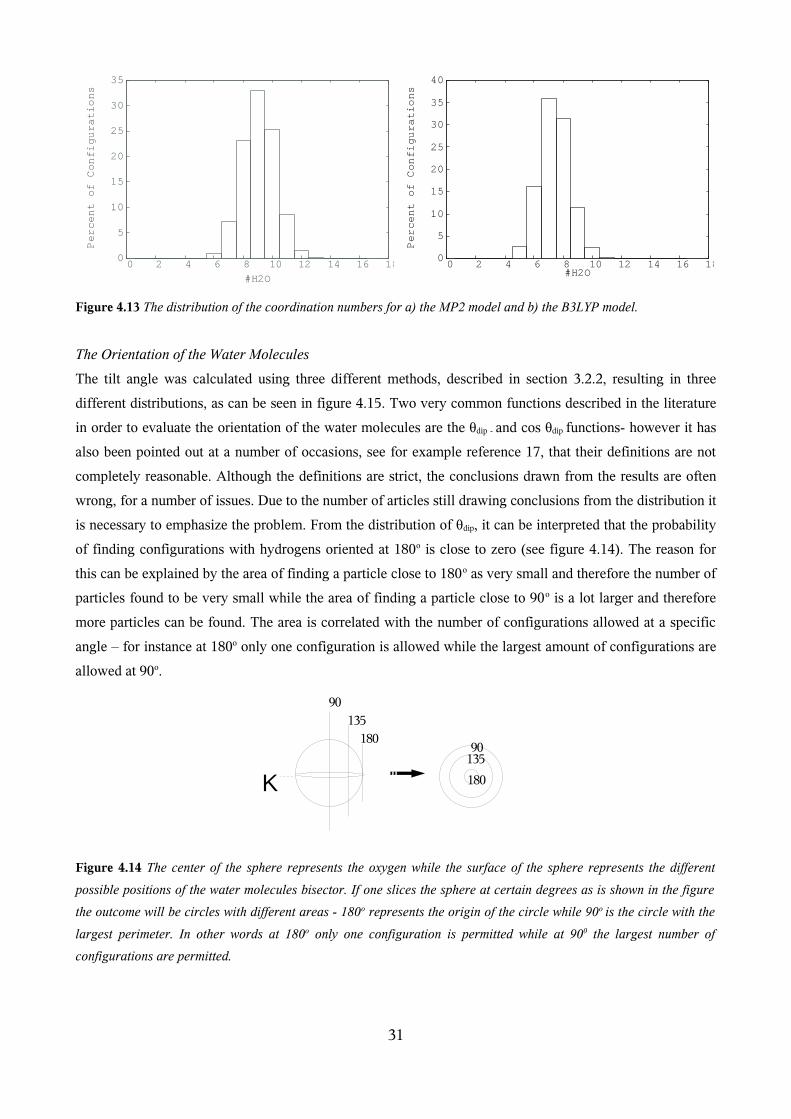
Figure 4.13 The distribution of the coordination numbers for a) the MP2 model and b) the B3LYP model.
The Orientation of the Water Molecules
The tilt angle was calculated using three different methods, described in section 3.2.2, resulting in three
different distributions, as can be seen in figure 4.15. Two very common functions described in the literature
in order to evaluate the orientation of the water molecules are the θdip - and cos θdip functions- however it has
also been pointed out at a number of occasions, see for example reference 17, that their definitions are not
completely reasonable. Although the definitions are strict, the conclusions drawn from the results are often
wrong, for a number of issues. Due to the number of articles still drawing conclusions from the distribution it
is necessary to emphasize the problem. From the distribution of θdip, it can be interpreted that the probability
of finding configurations with hydrogens oriented at 180o is close to zero (see figure 4.14). The reason for
this can be explained by the area of finding a particle close to 180o as very small and therefore the number of
particles found to be very small while the area of finding a particle close to 90o is a lot larger and therefore
more particles can be found. The area is correlated with the number of configurations allowed at a specific
angle – for instance at 180o only one configuration is allowed while the largest amount of configurations are
allowed at 90o.
Figure 4.14 The center of the sphere represents the oxygen while the surface of the sphere represents the different
possible positions of the water molecules bisector. If one slices the sphere at certain degrees as is shown in the figure
the outcome will be circles with different areas - 180o represents the origin of the circle while 90o is the circle with the
largest perimeter. In other words at 180o only one configuration is permitted while at 900 the largest number of
configurations are permitted.
31
180135
90
90135
180K
0
5
10
15
20
25
30
35
0 2 4 6 8 10 12 14 16 18
Percentof
Configurations
#H2O
0
5
10
15
20
25
30
35
40
0 2 4 6 8 10 12 14 16 18
Percentof
Configurations
#H2O
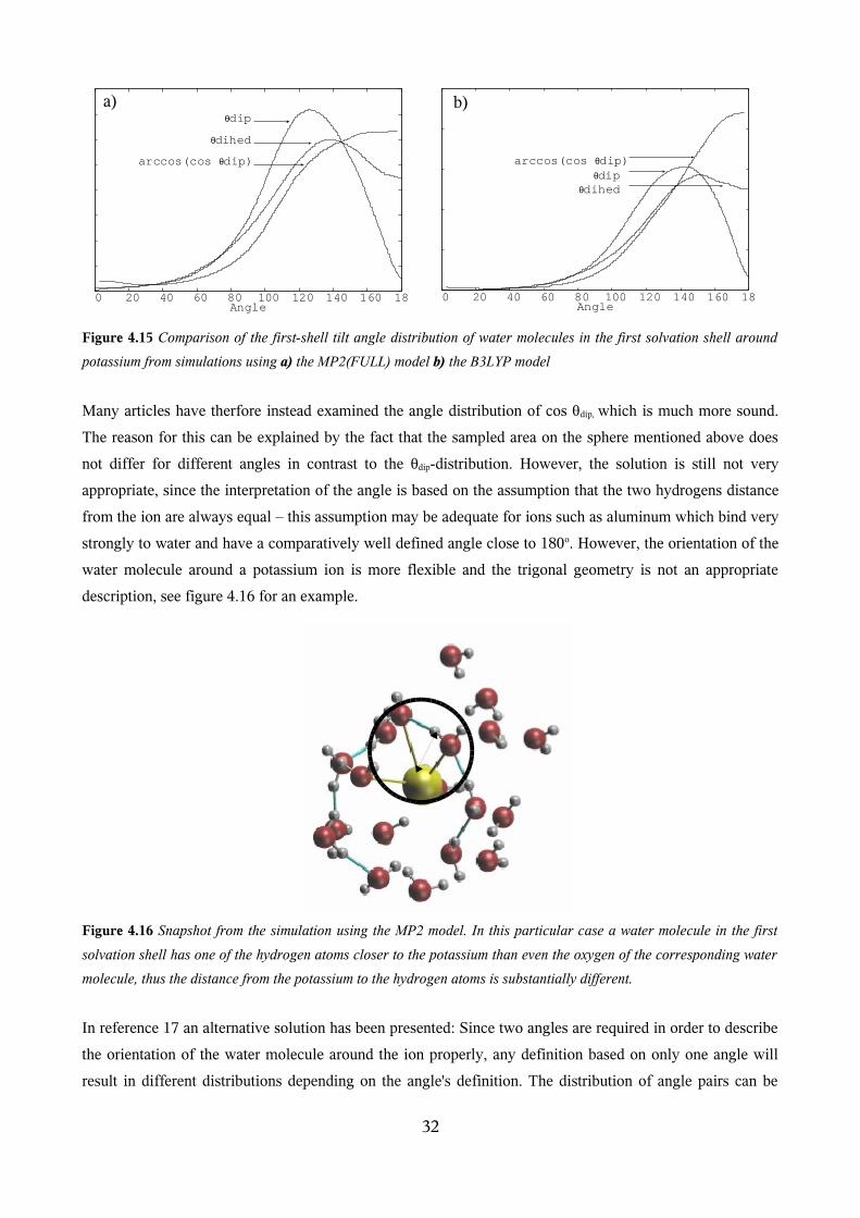
Figure 4.15 Comparison of the first-shell tilt angle distribution of water molecules in the first solvation shell around
potassium from simulations using a) the MP2(FULL) model b) the B3LYP model
Many articles have therfore instead examined the angle distribution of cos θdip, which is much more sound.
The reason for this can be explained by the fact that the sampled area on the sphere mentioned above does
not differ for different angles in contrast to the θdip-distribution. However, the solution is still not very
appropriate, since the interpretation of the angle is based on the assumption that the two hydrogens distance
from the ion are always equal – this assumption may be adequate for ions such as aluminum which bind very
strongly to water and have a comparatively well defined angle close to 180o. However, the orientation of the
water molecule around a potassium ion is more flexible and the trigonal geometry is not an appropriate
description, see figure 4.16 for an example.
Figure 4.16 Snapshot from the simulation using the MP2 model. In this particular case a water molecule in the first
solvation shell has one of the hydrogen atoms closer to the potassium than even the oxygen of the corresponding water
molecule, thus the distance from the potassium to the hydrogen atoms is substantially different.
In reference 17 an alternative solution has been presented: Since two angles are required in order to describe
the orientation of the water molecule around the ion properly, any definition based on only one angle will
result in different distributions depending on the angle's definition. The distribution of angle pairs can be
32
b)a)
0 20 40 60 80 100 120 140 160 180Angle
arccos(cos θdip)
θdihedθdip
0 20 40 60 80 100 120 140 160 180Angle
θdihed
arccos(cos θdip)
θdip
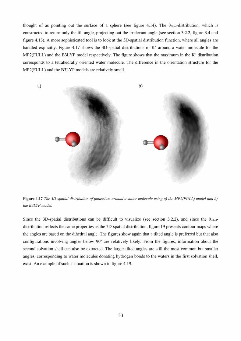
thought of as pointing out the surface of a sphere (see figure 4.14). The θdihed-distribution, which is
constructed to return only the tilt angle, projecting out the irrelevant angle (see section 3.2.2, figure 3.4 and
figure 4.15). A more sophisticated tool is to look at the 3D-spatial distribution function, where all angles are
handled explicitly. Figure 4.17 shows the 3D-spatial distributions of K+ around a water molecule for the
MP2(FULL) and the B3LYP model respectively. The figure shows that the maximum in the K+ distribution
corresponds to a tetrahedrally oriented water molecule. The difference in the orientation structure for the
MP2(FULL) and the B3LYP models are relatively small.
Figure 4.17 The 3D-spatial distribution of potassium around a water molecule using a) the MP2(FULL) model and b)
the B3LYP model.
Since the 3D-spatial distributions can be difficult to visualize (see section 3.2.2), and since the θdihed-
distribution reflects the same properties as the 3D-spatial distribution, figure 19 presents contour maps where
the angles are based on the dihedral angle. The figures show again that a tilted angle is preferred but that also
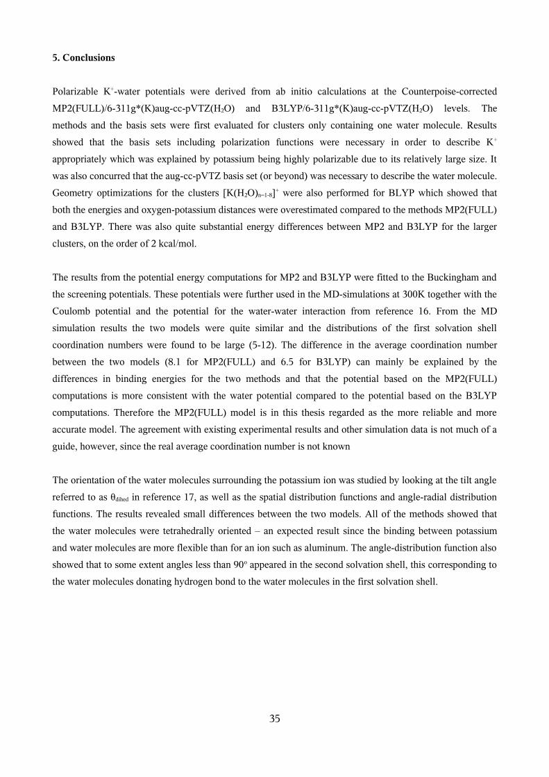
configurations involving angles below 90o are relatively likely. From the figures, information about the
second solvation shell can also be extracted. The larger tilted angles are still the most common but smaller
angles, corresponding to water molecules donating hydrogen bonds to the waters in the first solvation shell,
exist. An example of such a situation is shown in figure 4.19.
33
a) b)
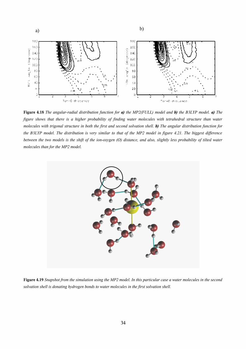
Figure 4.18 The angular-radial distribution function for a) the MP2(FULL) model and b) the B3LYP model. a) The
figure shows that there is a higher probability of finding water molecules with tetrahedral structure than water
molecules with trigonal structure in both the first and second solvation shell. b) The angular distribution function for
the B3LYP model. The distribution is very similar to that of the MP2 model in figure 4.21. The biggest difference
between the two models is the shift of the ion-oxygen (O) distance, and also, slightly less probability of tilted water
molecules than for the MP2 model.
Figure 4.19 Snapshot from the simulation using the MP2 model. In this particular case a water molecules in the second
solvation shell is donating hydrogen bonds to water molecules in the first solvation shell.
34
b)a)
5. Conclusions
Polarizable K+-water potentials were derived from ab initio calculations at the Counterpoise-corrected
MP2(FULL)/6-311g*(K)aug-cc-pVTZ(H2O) and B3LYP/6-311g*(K)aug-cc-pVTZ(H2O) levels. The
methods and the basis sets were first evaluated for clusters only containing one water molecule. Results
showed that the basis sets including polarization functions were necessary in order to describe K+
appropriately which was explained by potassium being highly polarizable due to its relatively large size. It
was also concurred that the aug-cc-pVTZ basis set (or beyond) was necessary to describe the water molecule.
Geometry optimizations for the clusters [K(H2O)n=1-8]+ were also performed for BLYP which showed that
both the energies and oxygen-potassium distances were overestimated compared to the methods MP2(FULL)
and B3LYP. There was also quite substantial energy differences between MP2 and B3LYP for the larger
clusters, on the order of 2 kcal/mol.
The results from the potential energy computations for MP2 and B3LYP were fitted to the Buckingham and
the screening potentials. These potentials were further used in the MD-simulations at 300K together with the
Coulomb potential and the potential for the water-water interaction from reference 16. From the MD
simulation results the two models were quite similar and the distributions of the first solvation shell
coordination numbers were found to be large (5-12). The difference in the average coordination number
between the two models (8.1 for MP2(FULL) and 6.5 for B3LYP) can mainly be explained by the
differences in binding energies for the two methods and that the potential based on the MP2(FULL)
computations is more consistent with the water potential compared to the potential based on the B3LYP
computations. Therefore the MP2(FULL) model is in this thesis regarded as the more reliable and more
accurate model. The agreement with existing experimental results and other simulation data is not much of a
guide, however, since the real average coordination number is not known
The orientation of the water molecules surrounding the potassium ion was studied by looking at the tilt angle
referred to as θdihed in reference 17, as well as the spatial distribution functions and angle-radial distribution
functions. The results revealed small differences between the two models. All of the methods showed that
the water molecules were tetrahedrally oriented – an expected result since the binding between potassium
and water molecules are more flexible than for an ion such as aluminum. The angle-distribution function also
showed that to some extent angles less than 90o appeared in the second solvation shell, this corresponding to
the water molecules donating hydrogen bond to the water molecules in the first solvation shell.
35
Future Work
The differences between the MP2(FULL) and B3LYP model lies not so much in the orientation as the
differences in distance and the average coordination number. In comparison to literature, the coordination
number of the MP2(FULL) model was closer to previous model studies than the B3LYP model except for
the results obtained with the Car-Parrinello method using the BLYP functional [27]. Interestingly the Car-
Parrinello method is the only other model which is based on DFT-calculations (BLYP). Since the Car-
Parrinello method using the BLYP functional gives an impressive water structure and since the B3LYP
model in this thesis was considered less accurate, it would be interesting to perform MD simulations using
the same type of water model as used in this study but based on BLYP – in order to see if the differences is
related to the DFT functionals or to the potential/method.
It would also be interesting to perform simulations by including other ions. How do anions, such as chlorine,
affect the water molecules surrounding the potassium ion? If one anion does not affect the water molecules,
will two, three or four ions affect a solution including 1024 water molecule?. Considering that the
experiments were done for much higher concentrations (3.2-53.7 molar ratio H2O/salt [3]), it would also be
intriguing to see if higher concentrations change the coordination number of the potassium ion.
Acknowledgments
I would first of all like to give my special thanks you to my supervisor, Daniel Spångberg, at the
Departments of Materials Chemistry. He has not only been a great source of inspiration, but he has also
helped and encouraged me a whole lot. I would also like to thank my supervisor, Professor Lars-Erik
Persson, at Department of Mathematics for giving me the opportunity to do my thesis in mathematics. A
great thank you to Kersti Hermansson for giving me the opportunity to do my thesis at the Department of
Materials Chemistry and for her remarks. Many thanks to the rest of the Theoretical Inorganic Chemistry
group for their great company and for making me feel like a part of the group.
36
7. References
[1] Doyle D. A., Cabral J. M., Pfuetzner R. A., Kuo A., Gulbis J. M., Cohen S. L., Chait B. T. and Mc
Kinnon R., Science 280, 69 (1998)
[2] Lide D. R., CRC Handbook of Chemistry and Physics 87th ed. CRC press Boca Raton, FL. 2005-6
[3] Ohtaki H. and Radnai R., Chem. Rev. 93 1157 (1993)
[4] Glezakou V. A., Chen Y., Fulton J. L., Schenter G. K. and Dang L. X., Theor. Chem. Acc. 115, 86
(2006)
[5] Leach A R, Molecular Modeling - Principles and Applications, 2nd ed. Harlow: Prentice Hall 2001
[6] Jensen F, Introduction to Computational Chemistry, New York: Wiley 1999
[7] J.A. Pople, J. Chem. Phys. 62, 2921 (1975)
[8] V. Rassolov, J.A. Pople, M. Ratner and T.L. Windus, J. Chem. Phys. 109, 1223 (1998)
[9] J-P. Blaudeau, M. P. McGrath, L.A. Curtiss and L. Radom, J. Chem. Phys. 107, 5016 (1997)
[10] T.H. Dunning, Jr. J. Chem. Phys. 90, 1007 (1989)
[11] Frenkel D. and Smit B.,Understanding Molecular Simulation: From Algorithms to Applications, 2nd
ed. San Diego: Academic Press 2002
[12] Allen M. P. and Tildesley D., Computer Simulation of Liquids, Oxford: Clarendon 1987
[13] M. W. Schmidt, K. K. Baldridge, J.A. Boatz, S.T. Elbert, M.S. Gordon, J. J. Jensen, S. Koseki, N.
Matsunaga, K.A. Nguyen, S. Su, et al., J. Comput. Chem. 14, 1347 (1993)
[14] Feller D., Glendening E. D., Woon D. E. and Feyereisen M. W., J. Chem. Phys. 103 3526 (1995)
[15] Ypot is an in-house program by Spånberg D., Uppsala University
[16] Spångberg D. and Hermansson K., to be published
[17] Spångberg D. and Hermansson K., J. Chem. Phys. 119, 7263 (2003)
[18] Spångberg D. and Hermansson K., J. Chem. Phys 120, 4289 (2002)
[19] Feller D., J. Chem. Phys. 96, 6104 (1992)
[20] Myoung Lee H., Kim J., Lee S., Jin Mhin B. and Kim K. S., J. Chem. Phys. 111 3995 (1999)
[21] Dzidic I. and Kebarle P., J. Phys. Chem., 74, 1466 (1970)
[22] Carillo-Tripp M., Saint-Martin H. and Ortega-Blake I., J. Chem. Phys. 118, 7062 (2003)
[23] Tongraar A. Liedl K. R. and Rode B. M., J. Phys. Chem. A 102,10340 (1998)
[24] Obst S. and Bradaczek H., J.Phys. Chem. 100, 15677 (1996)
[25] Chang T. M. and Dang L. X., J. Phys. Chem. B 103, 4724 (1999)
[26] Periole X., Allouche D., Daudey J. P. and Sanejouand Y. H., J. Phys. Chem. B 101, 5018 (1997)
[27] Ramaniah L. M., Bernasconi M. and Parrinello M., J. Chem. Phys. 111, 1587 (1999)
37
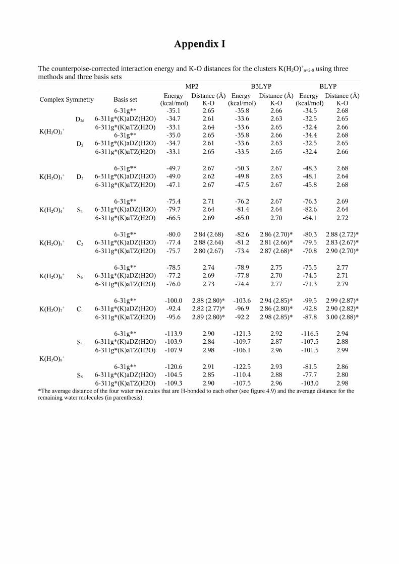
Appendix I
The counterpoise-corrected interaction energy and K-O distances for the clusters K(H2O)+n=2-8 using three
methods and three basis setsMP2 B3LYP BLYP
Complex Symmetry Basis setEnergy
(kcal/mol)Distance (Å)
K-OEnergy
(kcal/mol)Distance (Å)
K-OEnergy
(kcal/mol)Distance (Å)
K-O
K(H2O)2+
D2d
6-31g** -35.1 2.65 -35.8 2.66 -34.5 2.686-311g*(K)aDZ(H2O) -34.7 2.61 -33.6 2.63 -32.5 2.656-311g*(K)aTZ(H2O) -33.1 2.64 -33.6 2.65 -32.4 2.66
D2
6-31g** -35.0 2.65 -35.8 2.66 -34.4 2.686-311g*(K)aDZ(H2O) -34.7 2.61 -33.6 2.63 -32.5 2.656-311g*(K)aTZ(H2O) -33.1 2.65 -33.5 2.65 -32.4 2.66
K(H2O)3+ D3
6-31g** -49.7 2.67 -50.3 2.67 -48.3 2.686-311g*(K)aDZ(H2O) -49.0 2.62 -49.8 2.63 -48.1 2.646-311g*(K)aTZ(H2O) -47.1 2.67 -47.5 2.67 -45.8 2.68
K(H2O)4+ S4
6-31g** -75.4 2.71 -76.2 2.67 -76.3 2.696-311g*(K)aDZ(H2O) -79.7 2.64 -81.4 2.64 -82.6 2.646-311g*(K)aTZ(H2O) -66.5 2.69 -65.0 2.70 -64.1 2.72
K(H2O)5+ C2
6-31g** -80.0 2.84 (2.68) -82.6 2.86 (2.70)* -80.3 2.88 (2.72)*6-311g*(K)aDZ(H2O) -77.4 2.88 (2.64) -81.2 2.81 (2.66)* -79.5 2.83 (2.67)*6-311g*(K)aTZ(H2O) -75.7 2.80 (2.67) -73.4 2.87 (2.68)* -70.8 2.90 (2.70)*
K(H2O)6+ S6
6-31g** -78.5 2.74 -78.9 2.75 -75.5 2.776-311g*(K)aDZ(H2O) -77.2 2.69 -77.8 2.70 -74.5 2.716-311g*(K)aTZ(H2O) -76.0 2.73 -74.4 2.77 -71.3 2.79
K(H2O)7+ C1
6-31g** -100.0 2.88 (2.80)* -103.6 2.94 (2.85)* -99.5 2.99 (2.87)*6-311g*(K)aDZ(H2O) -92.4 2.82 (2.77)* -96.9 2.86 (2.80)* -92.8 2.90 (2.82)*6-311g*(K)aTZ(H2O) -95.6 2.89 (2.80)* -92.2 2.98 (2.85)* -87.8 3.00 (2.88)*
K(H2O)8+
S4
6-31g** -113.9 2.90 -121.3 2.92 -116.5 2.946-311g*(K)aDZ(H2O) -103.9 2.84 -109.7 2.87 -107.5 2.886-311g*(K)aTZ(H2O) -107.9 2.98 -106.1 2.96 -101.5 2.99
S8
6-31g** -120.6 2.91 -122.5 2.93 -81.5 2.866-311g*(K)aDZ(H2O) -104.5 2.85 -110.4 2.88 -77.7 2.806-311g*(K)aTZ(H2O) -109.3 2.90 -107.5 2.96 -103.0 2.98
*The average distance of the four water molecules that are H-bonded to each other (see figure 4.9) and the average distance for the remaining water molecules (in parenthesis).
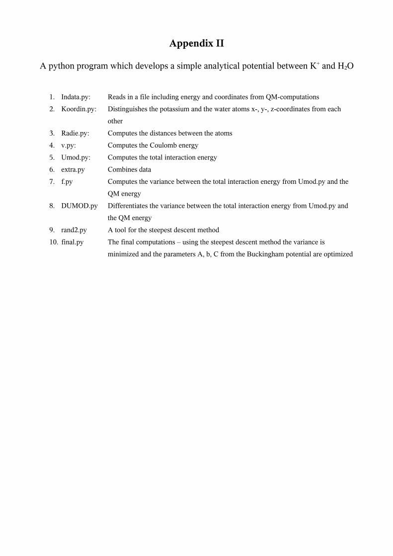
Appendix II
A python program which develops a simple analytical potential between K+ and H2O
1. Indata.py: Reads in a file including energy and coordinates from QM-computations
2. Koordin.py: Distinguishes the potassium and the water atoms x-, y-, z-coordinates from each
other
3. Radie.py: Computes the distances between the atoms
4. v.py: Computes the Coulomb energy
5. Umod.py: Computes the total interaction energy
6. extra.py Combines data
7. f.py Computes the variance between the total interaction energy from Umod.py and the
QM energy
8. DUMOD.py Differentiates the variance between the total interaction energy from Umod.py and
the QM energy
9. rand2.py A tool for the steepest descent method
10. final.py The final computations – using the steepest descent method the variance is
minimized and the parameters A, b, C from the Buckingham potential are optimized

1. Indata.py: Reads in a file including energy and coordinates from QM-computations. Separates the energy variable and the four atoms (K, O, H and H) coordinates.
def lasin(): f=open("h2ok.out2") #Opens the file with the QM computations en=[] co=[] co1=[] co2=[] co3=[]
while 1: x=f.readline() #Reads in line by line if not x: break en.append(x) # Defines an array including the energy f.readline() co.append(f.readline()) # Defines an array including the coordinates for the potassium f.readline() co1.append(f.readline()) #Defines an array including the coordinates for oxygen co2.append(f.readline()) #Defines an array including the coordinates for the first hydrogen atom co3.append(f.readline()) #Defines an array including the coordinates for the second hydrogen atom at=f.readline() return (en, co, co1, co2, co3)
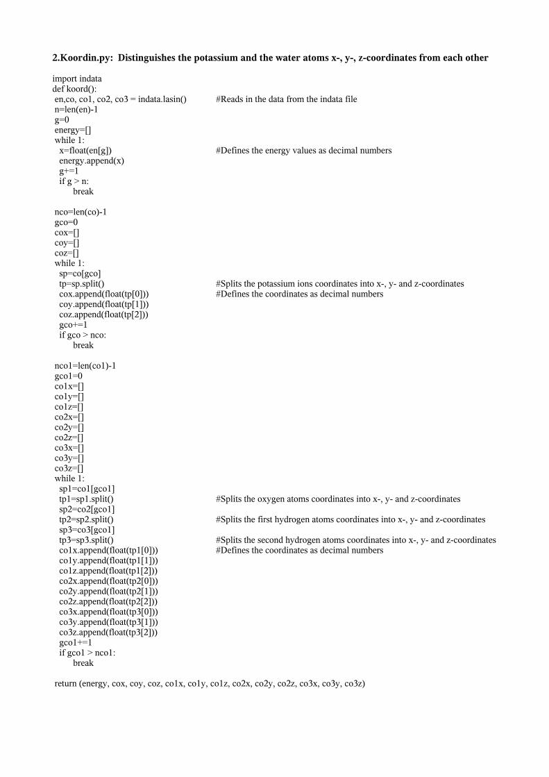
2.Koordin.py: Distinguishes the potassium and the water atoms x-, y-, z-coordinates from each other
import indatadef koord(): en,co, co1, co2, co3 = indata.lasin() #Reads in the data from the indata file n=len(en)-1 g=0 energy=[] while 1: x=float(en[g]) #Defines the energy values as decimal numbers energy.append(x) g+=1 if g > n: break
nco=len(co)-1 gco=0 cox=[] coy=[] coz=[] while 1: sp=co[gco] tp=sp.split() #Splits the potassium ions coordinates into x-, y- and z-coordinates cox.append(float(tp[0])) #Defines the coordinates as decimal numbers coy.append(float(tp[1])) coz.append(float(tp[2])) gco+=1 if gco > nco: break
nco1=len(co1)-1 gco1=0 co1x=[] co1y=[] co1z=[] co2x=[] co2y=[] co2z=[] co3x=[] co3y=[] co3z=[] while 1: sp1=co1[gco1] tp1=sp1.split() #Splits the oxygen atoms coordinates into x-, y- and z-coordinates sp2=co2[gco1] tp2=sp2.split() #Splits the first hydrogen atoms coordinates into x-, y- and z-coordinates sp3=co3[gco1] tp3=sp3.split() #Splits the second hydrogen atoms coordinates into x-, y- and z-coordinates co1x.append(float(tp1[0])) #Defines the coordinates as decimal numbers co1y.append(float(tp1[1])) co1z.append(float(tp1[2])) co2x.append(float(tp2[0])) co2y.append(float(tp2[1])) co2z.append(float(tp2[2])) co3x.append(float(tp3[0])) co3y.append(float(tp3[1])) co3z.append(float(tp3[2])) gco1+=1 if gco1 > nco1: break
return (energy, cox, coy, coz, co1x, co1y, co1z, co2x, co2y, co2z, co3x, co3y, co3z)
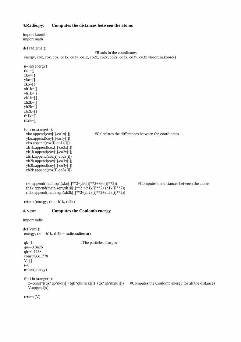
3.Radie.py: Computes the distances between the atoms
import koordinimport math
def radierna():#Reads in the coordinates
energy, cox, coy, coz, co1x, co1y, co1z, co2x, co2y, co2z, co3x, co3y, co3z =koordin.koord()
n=len(energy) rko=[] xko=[] yko=[] zko=[] xh1k=[] yh1k=[] zh1k=[] xh2k=[] yh2k=[] zh2k=[] rh1k=[] rh2k=[]
for i in xrange(n): xko.append(cox[i]-co1x[i]) #Calculates the differences between the coordinates yko.append(coy[i]-co1y[i]) zko.append(coz[i]-co1z[i]) xh1k.append(cox[i]-co2x[i]) yh1k.append(coy[i]-co2y[i]) zh1k.append(coz[i]-co2z[i]) xh2k.append(cox[i]-co3x[i]) yh2k.append(coy[i]-co3y[i]) zh2k.append(coz[i]-co3z[i])
rko.append(math.sqrt(xko[i]**2+yko[i]**2+zko[i]**2)) #Computes the distances between the atoms rh1k.append(math.sqrt(xh1k[i]**2+yh1k[i]**2+zh1k[i]**2)) rh2k.append(math.sqrt(xh2k[i]**2+yh2k[i]**2+zh2k[i]**2))
return (energy, rko, rh1k, rh2k)
4. v.py: Computes the Coulomb energy
import radie
def Vim(): energy, rko, rh1k, rh2k = radie.radierna()
qk=1. #The particles charges qo=-0.8476 qh=0.4238 const=331.778 V=[] i=0 n=len(energy)
for i in xrange(n): x=const*((qk*qo/rko[i])+(qk*qh/rh1k[i])+(qk*qh/rh2k[i])) #Computes the Coulomb energy for all the distances V.append(x)
return (V)

5. Umod.py: Computes the total interaction energyimport radieimport math
def umod(V, ako, bko, cko): energy, rko, rh1k, rh2k = radie.radierna()
n=len(energy) expo=[] r6=[] UMOD=[] f=0 for i in xrange(n): e=ako*math.exp(-bko*rko[i]) #Computes the Buckingham potential energy e2=cko/(rko[i]**6) UMOD.append(V[i]+e-e2) #Adds the Coulomb energy and the Buckingham potential return UMOD
6. extra.py Combines data
import vimport Umodimport radie
def ex(a, b, c):
V=v.Vim() UMOD=Umod.umod(V, a, b, c) energy, rko, rh1k, rh2k = radie.radierna() return (a, b, c, V, UMOD, energy)
7. f.py Computes the variance between the total interaction energy from Umod.py and the QM energy
import extraimport math
def F(a, b, c): a, b, c, V, UMOD, energy = extra.ex(a, b, c) n=len(UMOD) f=0 for ii in xrange(n): f+=((UMOD[ii]-energy[ii])**2)*math.exp(-energy[ii]) #Computes the variance for each distance and adds the
#terms func=f/(n**2) return func
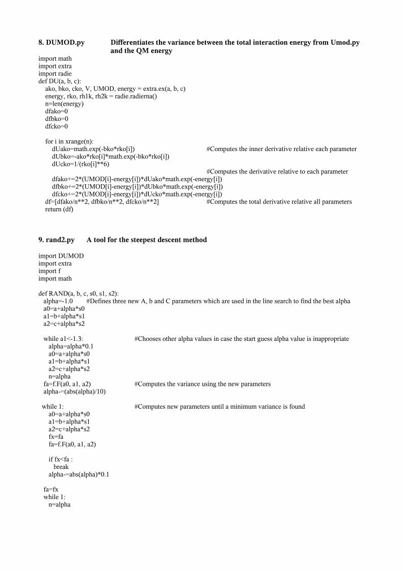
8. DUMOD.py Differentiates the variance between the total interaction energy from Umod.py and the QM energy
import mathimport extraimport radiedef DU(a, b, c): ako, bko, cko, V, UMOD, energy = extra.ex(a, b, c) energy, rko, rh1k, rh2k = radie.radierna() n=len(energy) dfako=0 dfbko=0 dfcko=0
for i in xrange(n): dUako=math.exp(-bko*rko[i]) #Computes the inner derivative relative each parameter dUbko=-ako*rko[i]*math.exp(-bko*rko[i]) dUcko=1/(rko[i]**6)
#Computes the derivative relative to each parameter dfako+=2*(UMOD[i]-energy[i])*dUako*math.exp(-energy[i]) dfbko+=2*(UMOD[i]-energy[i])*dUbko*math.exp(-energy[i]) dfcko+=2*(UMOD[i]-energy[i])*dUcko*math.exp(-energy[i]) df=[dfako/n**2, dfbko/n**2, dfcko/n**2] #Computes the total derivative relative all parameters return (df)
9. rand2.py A tool for the steepest descent method
import DUMODimport extraimport fimport math
def RAND(a, b, c, s0, s1, s2): alpha=-1.0 #Defines three new A, b and C parameters which are used in the line search to find the best alpha a0=a+alpha*s0 a1=b+alpha*s1 a2=c+alpha*s2
while a1<-1.3: #Chooses other alpha values in case the start guess alpha value is inappropriate alpha=alpha*0.1 a0=a+alpha*s0 a1=b+alpha*s1 a2=c+alpha*s2 n=alpha fa=f.F(a0, a1, a2) #Computes the variance using the new parameters alpha-=(abs(alpha)/10) while 1: #Computes new parameters until a minimum variance is found a0=a+alpha*s0 a1=b+alpha*s1 a2=c+alpha*s2 fx=fa fa=f.F(a0, a1, a2) if fx<fa : break alpha-=abs(alpha)*0.1
fa=fx while 1: n=alpha

alpha+=(abs(alpha)/10) a0=a+alpha*s0 a1=b+alpha*s1 a2=c+alpha*s2 fx=fa fa=f.F(a0, a1, a2) if fx<fa: break if alpha>-1e-10: break n=alpha
alpha=abs(alpha) if fx>fa: while 1: n=alpha alpha+=(abs(alpha)/10) a0=a+alpha*s0 a1=b+alpha*s1 a2=c+alpha*s2 fx=fa fa=f.F(a0, a1, a2) if fx<fa: break
a0=a+n*s0 a1=b+n*s1 a2=c+n*s2 fa=f.F(a0, a1, a2) nb=n+10 while 1: a0=a+(nb)*s0 a1=b+(nb)*s1 a2=c+(nb)*s2 fb=f.F(a0, a1, a2) if fa<fb: break nb=nb+10
nc=n-abs(n)*1e-6 aa=1 while 1: a0=a+(nc)*s0 a1=b+(nc)*s1 a2=c+(nc)*s2 fc=f.F(a0, a1, a2) if fa<fc: break nc=n-abs(n)*10**aa aa+=aa
return nc, n, nb #Returns the “favorite“ alpha value and two “extra values” - one lower and one higher
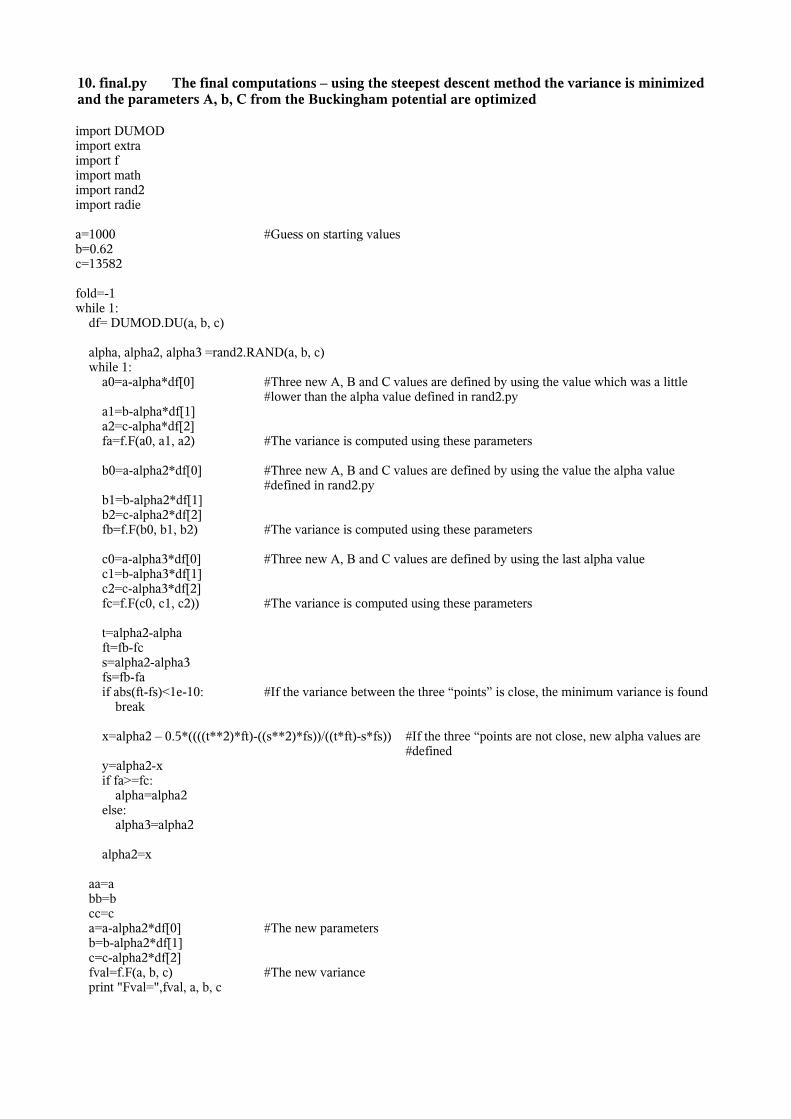
10. final.py The final computations – using the steepest descent method the variance is minimized and the parameters A, b, C from the Buckingham potential are optimized
import DUMODimport extraimport fimport mathimport rand2import radie
a=1000 #Guess on starting valuesb=0.62c=13582
fold=-1while 1: df= DUMOD.DU(a, b, c)
alpha, alpha2, alpha3 =rand2.RAND(a, b, c) while 1: a0=a-alpha*df[0] #Three new A, B and C values are defined by using the value which was a little
#lower than the alpha value defined in rand2.py a1=b-alpha*df[1] a2=c-alpha*df[2] fa=f.F(a0, a1, a2) #The variance is computed using these parameters
b0=a-alpha2*df[0] #Three new A, B and C values are defined by using the value the alpha value #defined in rand2.py
b1=b-alpha2*df[1] b2=c-alpha2*df[2] fb=f.F(b0, b1, b2) #The variance is computed using these parameters c0=a-alpha3*df[0] #Three new A, B and C values are defined by using the last alpha value c1=b-alpha3*df[1] c2=c-alpha3*df[2] fc=f.F(c0, c1, c2)) #The variance is computed using these parameters
t=alpha2-alpha ft=fb-fc s=alpha2-alpha3 fs=fb-fa if abs(ft-fs)<1e-10: #If the variance between the three “points” is close, the minimum variance is found break
x=alpha2 – 0.5*((((t**2)*ft)-((s**2)*fs))/((t*ft)-s*fs)) #If the three “points are not close, new alpha values are #defined
y=alpha2-x if fa>=fc: alpha=alpha2 else: alpha3=alpha2 alpha2=x
aa=a bb=b cc=c a=a-alpha2*df[0] #The new parameters b=b-alpha2*df[1] c=c-alpha2*df[2] fval=f.F(a, b, c) #The new variance print "Fval=",fval, a, b, c

if abs(fval-fold)<1e-9: #If the new variance is very close to the “old” variance, the minimum variance is #found
break fold=fval
print a, b, c, fval
a, b, c, V, UMOD, energy = extra.ex(a,b,c)energy, rko, rh1k, rh2k = radie.radierna()f=open ("h2ok.dat", "w")n=len(UMOD)-1i=0while 1: print >> f, UMOD[i], energy[i], rko[i] #The analytical potential is saved and can be visualized in the h2ok.dat file i+=1 if i>n: breakf.close()