Fast drift-approximated pricing in the BGM model Notation for BGM model In this section our notation of the BGM model is introduced. Consider a BGM model,M.1 Such a model features

It is demonstrated that the forward rates process discretized by a single timestep together with a separability assumption on the volatility function allowsfor representation by a low-dimensional Markov process. This in turn leads toefficient pricing by, for example, finite differences. We then develop a discret-ization based on the Brownian bridge that is especially designed to have highaccuracy for single time stepping. The scheme is proven to converge weaklywith order one. We compare the single time step method for pricing on a gridwith multi-step Monte Carlo simulation for a Bermudan swaption, reportinga computational speed increase by a factor 10, yet maintaining sufficientlyaccurate pricing.

1 Introduction

The BGM framework, developed by Brace, Gatarek and Musiela (1997),Miltersen, Sandmann and Sondermann (1997) and Jamshidian (1996, 1997), isnow one of the most popular models for pricing interest rate derivatives. In theBGM framework almost all prices are computed using Monte Carlo simulation.An advantage of Monte Carlo is its applicability to almost any product. However,it has the drawback of being computationally rather slow. In an attempt to limitthe computational time, Hunter, Jäckel and Joshi (2001a,b), Jäckel (2002, Section12.5) and Kurbanmuradov, Sabelfeld and Schoenmakers (1999, 2002) introduced

93

Fast drift-approximated pricing inthe BGM model

Raoul PieterszErasmus Research Institute of Management, Erasmus University Rotterdam, P.O. Box 1738, 3000

DR Rotterdam,The Netherlands

Antoon PelsserEconometric Institute, Faculty of Economics, Erasmus University Rotterdam, P.O. Box 1738, 3000

DR Rotterdam,The Netherlands

Marcel van RegenmortelProduct Development Group (HQ7011),ABN AMRO Bank, P.O. Box 283, 1000 EA Amsterdam,

The Netherlands

We are grateful for the comments of Tomas Björk, Dick Boswinkel, Marije Elkenbracht,Dariusz Gatarek, Lane Hughston, Dimitri Neumann, Martin Martens, Ton Vorst, Lars Wulf,and seminar participants at ABN AMRO Bank, ECFR, Mathematics in Finance 2002, SouthAfrica, and Quantitative Methods in Finance 2002, Australia. We thank Glyn Baker for the useof his hopscotch implementation. The first author is grateful for the financial support of theErasmus Center of Financial Research.

predictor-corrector drift approximations, which reduce the Monte Carlo stage tosingle time-step simulation.

This paper presents a significant addition to the single time step pricingmethod. We show that much more efficient numerical methods (either numericalintegration or finite differences) may be used at the cost of a minor additionalassumption, separability. The latter is a non-restrictive requirement on the formof the volatility function. The single time step together with separability rendersthe state of the BGM model completely determined by a low-dimensional Markovprocess. This enables efficient implementation.

We give an example of the fast single time step pricing framework for Bermudanswaptions. A comparison is made with prices obtained by least-squares multi-time step Monte Carlo simulation in the BGM model. This includes the use of theLongstaff and Schwartz (2001) method.

The computational speed increase achieved with the use of finite differencesfor BGM single time step pricing is the main result. This paper also contains twoother results:

The first result is a new time discretization using a Brownian bridge, as intro-duced in Section 3, which is proven to have least-squares error in a certain sense(to be defined) for single time step discretizations. In Section 4 it is shownnumerically that the Brownian bridge scheme outperforms (in the case ofsingle time steps) various other discretizations for the Libor-in-arrears densitytest. In the first part of Section 5, we prove theoretically that the Brownianbridge scheme converges weakly with order one when used for multi-time stepMonte Carlo. In the second part of Section 5, we compare the Brownian bridgescheme numerically with other discretizations for multi-time steps.

The second result is a method for measuring the accuracy of single timestepping. This is the timing inconsistency test as outlined in Section 8.

A further application of the Brownian bridge drift approximation is its use inthe likelihood ratio method. This method, introduced by Broadie and Glasserman(1996), efficiently estimates risk sensitivities for Monte Carlo pricing. Theparticular application of the likelihood ratio method to the Libor market modelhas been developed by Glasserman and Zhao (1999), who proposed the use ofdrift approximations.

The outline of this paper is as follows. After setting out some basic notationand the most important formulas for the BGM model, the single time step pricingframework is developed, various discretization schemes are discussed and theBrownian bridge scheme is introduced. The Brownian bridge scheme is theninvestigated theoretically and numerically for both single and multi-time steps,respectively. Next, the proposed framework is worked out for the one-factor case.This is followed by an example of the pricing of Bermudan swaptions, both for aone- and a two-factor model. A test is then developed to assess the quality ofsingle time steps. Finally, conclusions are drawn.

Raoul Pietersz, Antoon Pelsser and Marcel van Regenmortel

www.thejournalofcomputationalfinance.com Journal of Computational Finance

94

2 Notation for BGM model

In this section our notation of the BGM model is introduced.Consider a BGM model, M.1 Such a model features N forward rates, Li,

i = 1,…, N, where forward i accrues from time Ti to time Ti+1, 0 < T1 < … < TN+1.Define the accrual factor, δi, to be Ti+1 – Ti. Denote by Bi(t) the time-t price of adiscount bond that expires at time Ti. Bond prices and forward rates are linked bythe relation

Each forward rate is driven by a d-dimensional Brownian motion (where d is thenumber of stochastic factors in the BGM model), W, as follows:

µi(t)dt + σi(t) · dW(t) (1)

Here σi is the d-dimensional volatility vector, and µ~ i is the drift term, whose formwill in general depend on the choice of probability measure. Throughout, we usethe numeraire probability measure associated with the bond maturing at timeTN+1, the so called terminal measure. There is a specific reason why we use theterminal measure, and this is explained in Remark 2 of Section 3. For the termi-nal measure, the drift term will have the following form for i < N:

µi (t , Li +1,…, LN) (2)

For i = N the drift term is zero. This simply expresses the well-known fact that aforward rate is a martingale under its associated forward measure.

For the remainder of this paper it will be useful to have stochastic differentialequation (SDE) (1) in logarithmic form:

d log Li(t) = µi(t)dt + σi(t) · dWN+1(t),

µi(t) = µ~ i(t) – 1–2

σi(t)2

(3)

Last, we introduce the notion of all available forward rates at a given point intime. Define i(t) to be the smallest integer i such that t ≤ Ti. Define L to consist ofall forward rates that have not yet expired at time t, ie,

(4)L(t) = (Li(t)(t),…, LN (t))

δ σ σ

δk k k i

k kk i

L t t

L

( ) ( )

= +

= −⋅

+111

N

∑

dL t

L t

i

i

( )

( )=

11

+ =+

δi ii

i

L tB t

B t( )

( )

( )

Fast drift-approximated pricing in the BGM model

Volume 8/Number 1, Fall 2004 www.thejournalofcomputationalfinance.com

95

1 The construction of such a model may be found in, eg, Musiela and Rutkowski (1997),Pelsser (2000) or Brigo and Mercurio (2001).

3 Single time step method for pricing on a grid

The two key elements in the development of a method to price interest ratederivatives in the BGM model by low-dimensional finite differences are:

the forward rates process should be discretized by a single time step scheme;and

the volatility structure should be separable, which permits the dynamics of thesingle time step forward rates process to be represented by a low-dimensionalMarkov process.

3.1 Justification of the above assumptions

Because the forward rates are approximated by a single-step scheme, the modelwill in general no longer be arbitrage-free. This timing inconsistency is addressedin Section 8, where it is shown that its impact is negligible for most cases.The single-step approximation is accurate enough for the pricing of derivatives,as shown numerically in Section 7. At the end of this section we introduce anovel discretization scheme based on the Brownian bridge that is especiallydesigned for single time stepping. Its superiority (for single time steps only) overother discretizations is established in Section 4.

We proceed by first introducing notation for the single step-approximatedforward rates process. This is followed by a statement of the separability assump-tion, after which we establish the low-dimensional Markov representation result.Single time step discretizations are then discussed, and we end by consideringmethods for pricing American style options with Monte Carlo methods.

3.2 Notation

We assume as given a time discretization τ1 < … < τJ. Define Zi(u, v) = ∫u

vσi(t) ·

dWN+1(t). Given a scheme for the log rates

(5)log Li(τj+1) = log Li(τj) + Di (τj, τj+1, L(τj), Z(τj, τj+1)) + Zi(τj, τj+1)

then denote by

LiA(t) = Li(0) expDi(0, t, L(0), Z(0, t)) + Zi(0, t)

its single time step-approximated equivalent. Here D stands for “drift approxi-mation” and it is determined by the scheme applied, which may be the Euler,the predictor-corrector or the Brownian bridge scheme. These schemes will beelaborated on at the end of this section. The A in LA stands for “approximated”.The vector Z is defined by analogy with L in Equation (4).

3.3 Separability

DEFINITION 1 (SEPARABILITY) A collection of instantaneous volatility functionsσi : [0, Ti] → d, i = 1,…, N, is called “separable” if there exists a vector-valued



96

function σ : [0, T ] → d and vectors vi ∈d, i = 1,…, N, such that

(6)σi(t) = vi σ(t)

(no vector product; entry-by-entry multiplication) for 0 ≤ t ≤ Ti, i = 1,…, N.

Separability appears regularly in the context of requiring a process to be Markov.We mention three examples. First, we mention Ritchken and Sankarasubra-manian (1995, Proposition 2.1). Working in the HJM model (Heath, Jarrow andMorton, 1992), they show that separability is a necessary and sufficient conditionon the volatility structure such that the dynamics of the term structure may berepresented by a two-dimensional Markov process. Second, we mention theWiener chaos expansion framework of Hughston and Rafailidis (2002). In thisframework any interest rate model is completely characterized by its so-calledWiener chaos expansion. The n th chaos expansion is represented by a functionφn : +

n → that satisfies certain integrability conditions. If all φn are separable,the resulting interest rate model turns out to be Markov. Third, we mention thefinite-dimensional Markov realizations for stochastic volatility forward ratemodels (see Björk, Landén and Svensson, 2002). Here a necessary condition fora stochastic volatility model to have a finite-dimensional Markov realization isthat the drift term and each component of the volatility term in the Stratonovichrepresentation of the short rate SDE should be a sum of functions that are sepa-rable in time to expiry and the stochastic volatility driver.

We give an example of a separable volatility function in the case of a one-factor model (d = 1).

Example (mean-reversion) Following De Jong, Driessen and Pelsser (2002), theinstantaneous volatility may be specified as

(7)σi(t) = γi e–κ(Ti – t)

The constant κ is usually referred to as the mean-reversion parameter.

3.4 Single time step method

The following proposition shows that a single time step plus separability yieldslow-dimensional representability.

PROPOSITION 1 Suppose that M is a d-factor BGM model, for which the instan-taneous volatility structure is separable. Then the single time step discretizedforward rates process may be represented by a d-dimensional Markov process.

PROOF Define the Markov process X : [0, T ] → d by

X W( ) ( ) ( )t s sN

t

= +∫ σ d 1

0



97

(entry-by-entry multiplication) where σ is as in Definition 1. Then the single timestep process LA : [0, T ] → (0, ∞)n– i(t)+1 at time t satisfies

(8)LiA(t) = Li(0) expDi(0, t, L(0), vX(t)) + vi · X(t)

Here Di is defined implicitly by Equation (5) and v is a matrix of which row i isvi. The claim follows, bar a clarifying remark:

The second term in the exponent of Equation (8) is exactly equal to the sto-chastic part occurring in the BGM SDE (1), in virtue of the separability of thevolatility structure:

where the notation of Definition 1 has been used.

REMARK 1 The vector of single time-stepped rates may be considered (if separa-bility holds) to be a time-dependent function of the Markov process X, ie,

LA(t) = f (t, X(t))

for some function f. Hunt, Kennedy and Pelsser (2000, Theorem 1) showed thatthis is impossible to achieve for the true BGM forward rates themselves in thecase when X is one-dimensional and under some technical restrictions.

Another essential building block for the fast single time step pricing framework isuse of the terminal measure. This is explained in the following remark.

REMARK 2 (Choice of numeraire) For the workings of the fast single time steppricing algorithm it is essential that the terminal measure be used. This isexplained as follows. As proven in Proposition 1, the time-t single time-steppedforward rates are fully determined by X(t). This result holds for any choice ofmeasure or numeraire. However, for the terminal numeraire, the value of thenumeraire at time t is fully determined by the forward rate values at time t, butthis does not hold in the case of, for example, the spot numeraire, in that thelatter is generally determined by bond values observed at earlier times. The spotnumeraire B0 rolls its holdings over by the spot Libor account. Its time-Ti value is

Put in another way, the value of the spot numeraire is path-dependent, whereas

B TB T

Ti

j jj

i0

11

0

10( )

( ), := =

−=∏

σ σiN

t

i

tN

i

s s v s s

t

( ) ( ) ( ) ( )

( )

⋅ = ( ) ⋅

= ⋅

+ +∫ ∫d dW W

v X

1

0 0

1



98

that of the terminal numeraire is not. For pricing on a grid it is essential that thenumeraire value is known given the value of X(t). Therefore the fast single timestep framework requires the use of the terminal numeraire.

3.5 Valuation of interest rate derivatives with the single time step method

Interest rate derivatives with mild path-dependency may be valued by numericalintegration, by a lattice/tree or by finite differences, provided that the single time-stepped rates are used and the separability assumption holds. The derivatives thatmay be valued include, but are not restricted to: caps, floors, European andBermudan swaptions, trigger swaps and discrete barrier caps.

3.6 Discretizations

We discuss four time-discrete approximation schemes of the log BGM SDE (3):

Euler; predictor-corrector; Milstein second-order scheme; and Brownian bridge.

The notation (Equation (5)) for a discretization of SDE (3) is recalled here:

log Li(τj+1) = log Li(τj) + Di(τj, τj+1, L(τj), Z(τj, τj+1)) + Zi(τj, τj+1)

We implicitly define D~

by

Di (τj, τj+1, L(τj), Z(τj, τj+1)) = D~

i(τj, τj+1, L(τj), Z(τj, τj+1))

so as to remove the term common to the Euler, predictor-corrector and Brownianbridge discretizations.

3.6.1 Euler discretizationThe Euler discretization (see, for example, Kloeden and Platen (1999, Equation(9.3.1))) sets

Di (τj, τj+1, L(τj), Z(τj, τj+1)) =

3.6.2 Predictor-corrector discretizationThe predictor-corrector discretization was introduced to the setting of Libormarket models by Hunter, Jäckel and Joshi (2001a). The key idea is to use pre-dicted information to more accurately estimate the contribution of the drift to the

Lk k j kδ τ σ τ( ) (− jj i j

k k jk i

N

jL

) ( )

( )

⋅

+

−

= ++∑

σ τ

δ ττ τ

111 jj( )

−+

∫1

2

21

στ

τ

i s s

j

j

( ) d



99

increment of the log rate. For the terminal measure, an iterative procedure may beapplied that loops from the terminal forward rate, N, to the spot Libor rate, i(t).Initially, we set D

~N (τj, τj+1, L(τj), Z(τj, τj+1)) = 0. Then, for i = N – 1, …, i(t),

Di (τj , τj+1, L(τj), Z(τj , τj+1)) =

with Lk(τj+1) dependent on Lm(τj) and Zm(τj, τj+1), m = k + 1,…, N.

3.6.3 Milstein discretizationThe second-order Milstein scheme (see, for example, Kloeden and Platen (1999,Equation (14.2.1))) was introduced to the setting of Libor market models in theseries of papers by Glasserman and Merener (2003a,b and 2004). Moreover,these papers extended the convergence results to the case of jump–diffusion withthinning, which is key to the development of the jump–diffusion Libor marketmodel. Also, these papers considered discretizations in various different sets ofstate variables, such as forward rates, log-forward rates, relative discount bondprices and log-relative discount bond prices. In Glasserman and Merener (2003b,2004) it is shown numerically that the time-discretization bias of the log-Eulerscheme is less than the bias of other discretizations, for example, in terms of thebonds. The results of Glasserman and Merener thus justify the log-type discret-ization (5) used in the present work.

The Milstein scheme can indeed be used to obtain a single time step discret-ization of the forward rates process – and hence it may be applied to the singletime step pricing framework – but it is not particularly suited to single large timesteps, as shown in the numerical comparisons for single time step accuracy inSection 4. Therefore we omit here the exact form of the scheme.

3.6.4 Brownian bridge discretizationHere we develop a novel discretization for the drift term. The idea is to calculatethe expectation of the drift integral given the (time-changed) Wiener increment.

Di (τj , τj+1, L(τj), Z(τj , τj+1)) =

(9)

The Brownian bridge discretization is superior when a single time step is applied.

N kδ+− 1

LL s s s

L s

k k i

k kj j j

k

( ) ( ) ( )

( )( ), ( , )

σ σ

δτ τ τ

⋅

+ +1

1F Z== +∑∫

+

i

N

j

j

1

1

τ

τ

Lk k j kδ τ σ( )−

1

2

(( ) ( )

( )

( ) ( )τ σ τ

δ τ

δ τ σ τj i j

k k j

k k j k j

L

L⋅

++ + +

1

1

2

1 1 ⋅⋅

+

+

+= += +∑∑

σ τ

δ τi j

k k jk i

N

k i

N

L

( )

( )

1

111 1

×

−( )+τ τj j1



100

This is shown theoretically and numerically in Section 4. Viewed as a numericalscheme for multi-step discretizations, it converges weakly with order one, as willbe shown in the first part of Section 5. In the multi-step Monte Carlo numericalexperiments of the second part of Section 5, we show that the bias is significantlyless than for the Euler discretization.

In the remainder of this section, we first show how expression (9) can be cal-culated in practice, and, second, we establish that the Brownian bridge schemehas least-squares error (in a yet to be defined sense).

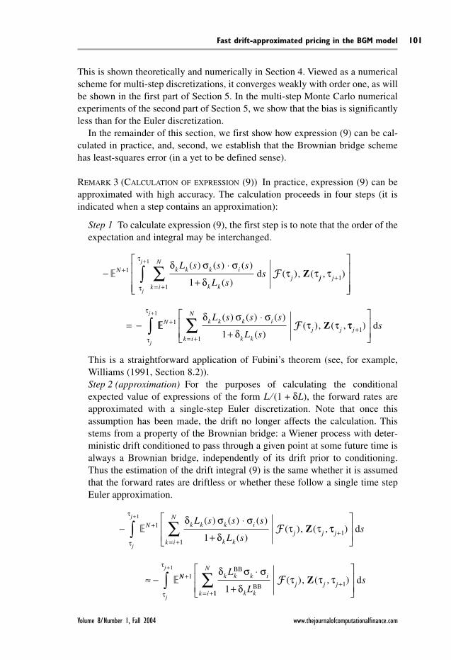
REMARK 3 (CALCULATION OF EXPRESSION (9)) In practice, expression (9) can beapproximated with high accuracy. The calculation proceeds in four steps (it isindicated when a step contains an approximation):

Step 1 To calculate expression (9), the first step is to note that the order of theexpectation and integral may be interchanged.

This is a straightforward application of Fubini’s theorem (see, for example,Williams (1991, Section 8.2)).Step 2 (approximation) For the purposes of calculating the conditionalexpected value of expressions of the form L ⁄ (1 + δL), the forward rates areapproximated with a single-step Euler discretization. Note that once thisassumption has been made, the drift no longer affects the calculation. Thisstems from a property of the Brownian bridge: a Wiener process with deter-ministic drift conditioned to pass through a given point at some future time isalways a Brownian bridge, independently of its drift prior to conditioning.Thus the estimation of the drift integral (9) is the same whether it is assumedthat the forward rates are driftless or whether these follow a single time stepEuler approximation.

−⋅

++

N k k k i

k kj j

L s s s

L s1

1

δ σ σ

δτ τ

( ) ( ) ( )

( )( ), ( ,F Z ττ

τ

τ

j

k i

N

j

j

s+= +∑∫

≈ −

+

11

1

) d

NN k k k i

k kj j j

k i

L

L

++

= +

⋅

+1

11

δ σ σ

δτ τ τ

BB

BBF ( ), ( , )Z

11

1 N

j

j

s∑∫

+

τ

τ

d

−⋅

++

N k k k i

k kj

L s s s

L ss1

1

δ σ σ

δτ τ

( ) ( ) ( )

( )( ), (d F Z jj j

k i

N

j

j

, )ττ

τ

+= +∑∫

+

= −

11

1

N k k k i

k kj j

L s s s

L s+ ⋅

+1

1

δ σ σ

δτ τ

( ) ( ) ( )

( )( ), ( ,F Z ττ

τ

τ

j

k i

N

j

j

s+= +∑∫

+

11

1

) d



101

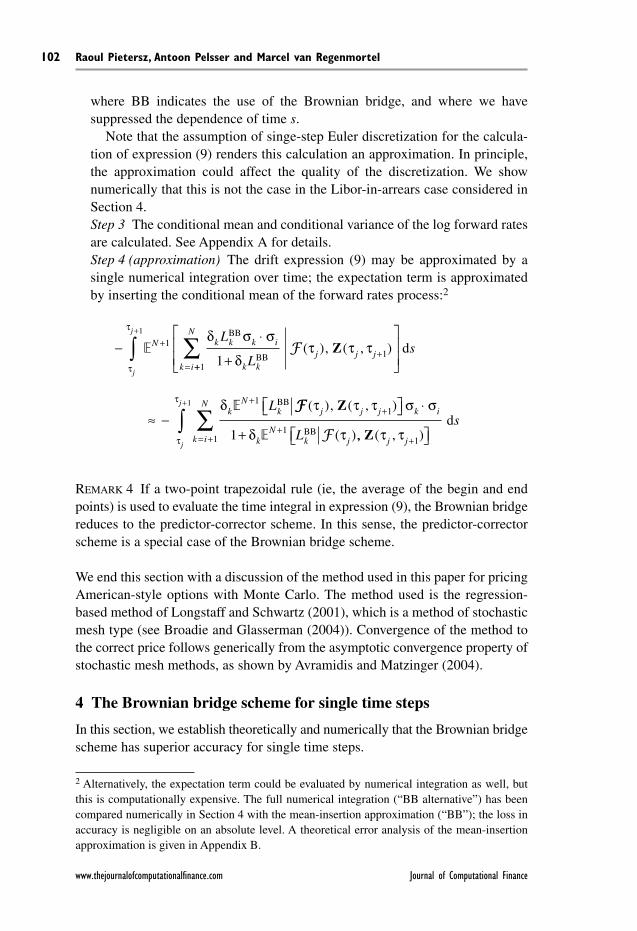
where BB indicates the use of the Brownian bridge, and where we havesuppressed the dependence of time s.

Note that the assumption of singe-step Euler discretization for the calcula-tion of expression (9) renders this calculation an approximation. In principle,the approximation could affect the quality of the discretization. We shownumerically that this is not the case in the Libor-in-arrears case considered inSection 4.Step 3 The conditional mean and conditional variance of the log forward ratesare calculated. See Appendix A for details.Step 4 (approximation) The drift expression (9) may be approximated by asingle numerical integration over time; the expectation term is approximatedby inserting the conditional mean of the forward rates process:2

REMARK 4 If a two-point trapezoidal rule (ie, the average of the begin and endpoints) is used to evaluate the time integral in expression (9), the Brownian bridgereduces to the predictor-corrector scheme. In this sense, the predictor-correctorscheme is a special case of the Brownian bridge scheme.

We end this section with a discussion of the method used in this paper for pricingAmerican-style options with Monte Carlo. The method used is the regression-based method of Longstaff and Schwartz (2001), which is a method of stochasticmesh type (see Broadie and Glasserman (2004)). Convergence of the method tothe correct price follows generically from the asymptotic convergence property ofstochastic mesh methods, as shown by Avramidis and Matzinger (2004).

4 The Brownian bridge scheme for single time steps

In this section, we establish theoretically and numerically that the Brownian bridgescheme has superior accuracy for single time steps.

−⋅

++

+=

N k k k i

k kj j j

k i

L

L

11

1

δ σ σ

δτ τ τ

BB

BBF ( ), ( , )Z

++

+

∑∫

≈ −

+

1

1

1 N

kN

k

j

j

s

L

τ

τ

δ

d

BB FFF

( ), ( , )

( )

τ τ τ σ σ

δ τ

j j j k i

kN

k jL

Z +

+

⋅

+

1

11 BB ,, ( , )Z τ ττ

τ

j jk i

N

j

j

s+= +

∑∫+

11

1

d



102

2 Alternatively, the expectation term could be evaluated by numerical integration as well, butthis is computationally expensive. The full numerical integration (“BB alternative”) has beencompared numerically in Section 4 with the mean-insertion approximation (“BB”); the loss inaccuracy is negligible on an absolute level. A theoretical error analysis of the mean-insertionapproximation is given in Appendix B.

4.1 Theoretical result

Consider a stochastic differential equation of the form

(10)dX(t) = µ(t, X(t))dt + σ(t) dW(t)

Note that the BGM log SDE (3) is of the above form. We consider a certain classof discretizations:

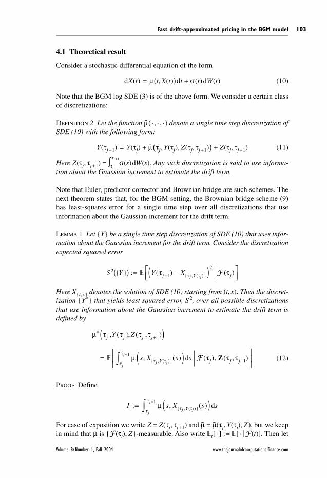
DEFINITION 2 Let the function µ( · , · , · ) denote a single time step discretization ofSDE (10) with the following form:

(11)Y(τj+1) = Y(τj) + µ(τj, Y(τj), Z(τj, τj+1)) + Z(τj, τj+1)

Here Z(τj, τj+1) = ∫τi

τi+1

σ(s)dW(s). Any such discretization is said to use informa-tion about the Gaussian increment to estimate the drift term.

Note that Euler, predictor-corrector and Brownian bridge are such schemes. Thenext theorem states that, for the BGM setting, the Brownian bridge scheme (9)has least-squares error for a single time step over all discretizations that useinformation about the Gaussian increment for the drift term.

LEMMA 1 Let Y be a single time step discretization of SDE (10) that uses infor-mation about the Gaussian increment for the drift term. Consider the discretizationexpected squared error

Here Xt, x denotes the solution of SDE (10) starting from (t, x). Then the discret-ization Y* that yields least squared error, S2, over all possible discretizationsthat use information about the Gaussian increment to estimate the drift term isdefined by

(12)

PROOF Define

For ease of exposition we write Z = Z(τj, τj+1) and µ = µ(τj, Y(τj), Z), but we keepin mind that µ is F(τj), Z-measurable. Also write t[ · ] := [ ·F(t)]. Then let

I s X s sj j

j

j

Y: , ( ) , ( )= ( )+∫ µ τ ττ

τd

1

µ τ τ τ τ

µ τ τ

*

, ( )

, ( ), ( , )

,

j j j j

Y

Y Z

s Xj j

+( )

=

1

(( ) ( ), ( , )s sj

j

j j j( )

+∫ +dτ

ττ τ τ1

1F Z

S Y Y Xj Y jj j

21

2 : ( ) ( ) , ( )( ) = −( )

+ τ ττ τ F



103

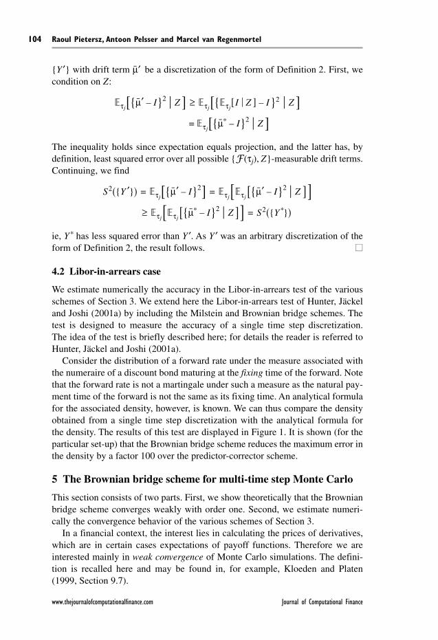
Y ′ with drift term µ′ be a discretization of the form of Definition 2. First, wecondition on Z:

τj[µ′ – I2Z ] ≥ τj[τj[ I Z ] – I2 Z ]

= τj[µ* – I2Z ]The inequality holds since expectation equals projection, and the latter has, bydefinition, least squared error over all possible F(τj), Z-measurable drift terms.Continuing, we find

S2(Y ′) = τj[µ′ – I2] = τj[τj [µ′ – I2Z ]]≥ τj[τj [µ* – I2Z ]] = S2(Y*)

ie, Y* has less squared error than Y ′. As Y ′ was an arbitrary discretization of theform of Definition 2, the result follows.

4.2 Libor-in-arrears case

We estimate numerically the accuracy in the Libor-in-arrears test of the variousschemes of Section 3. We extend here the Libor-in-arrears test of Hunter, Jäckeland Joshi (2001a) by including the Milstein and Brownian bridge schemes. Thetest is designed to measure the accuracy of a single time step discretization.The idea of the test is briefly described here; for details the reader is referred toHunter, Jäckel and Joshi (2001a).

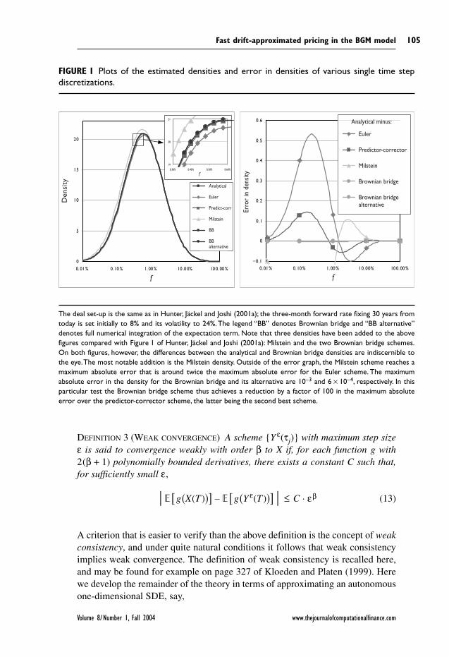
Consider the distribution of a forward rate under the measure associated withthe numeraire of a discount bond maturing at the fixing time of the forward. Notethat the forward rate is not a martingale under such a measure as the natural pay-ment time of the forward is not the same as its fixing time. An analytical formulafor the associated density, however, is known. We can thus compare the densityobtained from a single time step discretization with the analytical formula forthe density. The results of this test are displayed in Figure 1. It is shown (for theparticular set-up) that the Brownian bridge scheme reduces the maximum error inthe density by a factor 100 over the predictor-corrector scheme.

5 The Brownian bridge scheme for multi-time step Monte Carlo

This section consists of two parts. First, we show theoretically that the Brownianbridge scheme converges weakly with order one. Second, we estimate numeri-cally the convergence behavior of the various schemes of Section 3.

In a financial context, the interest lies in calculating the prices of derivatives,which are in certain cases expectations of payoff functions. Therefore we areinterested mainly in weak convergence of Monte Carlo simulations. The defini-tion is recalled here and may be found in, for example, Kloeden and Platen(1999, Section 9.7).



104

DEFINITION 3 (WEAK CONVERGENCE) A scheme Y ε(τj) with maximum step sizeε is said to convergence weakly with order β to X if, for each function g with2(β + 1) polynomially bounded derivatives, there exists a constant C such that,for sufficiently small ε,

(13) [g(X(T ))] – [g(Y ε(T ))] ≤ C · εβ

A criterion that is easier to verify than the above definition is the concept of weakconsistency, and under quite natural conditions it follows that weak consistencyimplies weak convergence. The definition of weak consistency is recalled here,and may be found for example on page 327 of Kloeden and Platen (1999). Herewe develop the remainder of the theory in terms of approximating an autonomousone-dimensional SDE, say,



105

FIGURE 1 Plots of the estimated densities and error in densities of various single time stepdiscretizations.

0

5

10

15

20

0. 01 % 0. 10 % 1. 00 % 10 .0 0% 10 0. 00 %

f

S

19

20

21

0.30% 0.40% 0.50% 0.60%

f

–0.1

0

0.1

0.2

0.3

0.4

0.5

0.6

0.01% 0.10% 1.00% 10.00% 100.00%

f

Den

sity Analytical

Euler

Predict-corr

Milstein

BB

BBalternative

Erro

r in

den

sity

Analytical minus:

Euler

Predictor-corrector

Milstein

Brownian bridge

Brownian bridgealternative

The deal set-up is the same as in Hunter, Jäckel and Joshi (2001a); the three-month forward rate fixing 30 years fromtoday is set initially to 8% and its volatility to 24%.The legend “BB” denotes Brownian bridge and “BB alternative”denotes full numerical integration of the expectation term. Note that three densities have been added to the abovefigures compared with Figure 1 of Hunter, Jäckel and Joshi (2001a): Milstein and the two Brownian bridge schemes.On both figures, however, the differences between the analytical and Brownian bridge densities are indiscernible tothe eye.The most notable addition is the Milstein density. Outside of the error graph, the Milstein scheme reaches amaximum absolute error that is around twice the maximum absolute error for the Euler scheme. The maximumabsolute error in the density for the Brownian bridge and its alternative are 10–3 and 6 × 10–4, respectively. In thisparticular test the Brownian bridge scheme thus achieves a reduction by a factor of 100 in the maximum absoluteerror over the predictor-corrector scheme, the latter being the second best scheme.

dX(t) = a(X(t))dt + b(X(t))dW(t), X(0) deterministic (14)

However, the theory holds in more general cases too.

DEFINITION 4 (WEAK CONSISTENCY) A scheme Y ε(τj) with maximum step size εis weakly consistent if there exists a function c = c(ε) with

(15)limε↓0

c(ε) = 0

such that

(16)

and

(17)

Here F(t) is the filtration generated by the Brownian motion driving SDE (14).

Kloeden and Platen prove the following theorem (see Theorem 9.7.4 of Kloedenand Platen (1999)) linking weak consistency to weak convergence.

THEOREM 1 (LINKING WEAK CONSISTENCY TO WEAK CONVERGENCE) Suppose thata and b of Equation (14) are four times continuously differentiable with poly-nomial growth and uniformly bounded derivatives. Let Y ε(τj) be a weaklyconsistent scheme with equitemporal steps ∆τj = ε and initial value Y ε(0) = X(0)which satisfies the moment bounds

and

(18)

where c(ε) is as in Definition 4. Then Y ε converges weakly to X.

1

1

6

ετ τ εε εY Y cj j( ) ( ) ( )+ −

≤

max ( ) ( ) , , ,j

j

q qY K X qε τ

2 21 0 1 2

≤ +( ) = ……

1

1 1∆τ

τ τ τ τε ε ε ε

j

j j j jY Y Y Y( ) ( ) ( ) ( ) (+ +− − F ττ j )

−

( ) ( ) ( )b Y b Y cj jε ετ τ ε( ) ( )

≤2

Y Y

a Yj j

jj j

ε εε

τ τ

ττ τ

( ) ( )( ) ( )

+ −

− ( )1

∆F

22

≤ c( )ε



106

In the proposition below we show that the Brownian bridge scheme with theproposed calculation method is weakly consistent. The above theorem then allowsus to deduce that the Brownian bridge scheme converges weakly.

PROPOSITION 2 (BROWNIAN BRIDGE SCHEME IS WEAKLY CONSISTENT) Assume thatthe volatility functions σi( · ) are piecewise analytical on the model horizon [0, T].Then the Brownian bridge scheme defined by Equation (9) and by the four-stepcalculation method described in Remark 3 is weakly consistent with the forwardrates process defined in Equation (3).

PROOF Without loss of generality, we may assume that the volatility functions areanalytical. Otherwise, due to the piecewise property of the volatility functions,we can break up the problem into sub-problems for which each has analyticalvolatility functions. Note also that all derivatives of the volatility functions arebounded because the interval [0, T ] is compact.

We need only verify the consistency Equation (16) for the drift term. Toachieve this, define for i and for all τ ∈[0, T ] and for all L the functionfi,τ,L : [0, T – τ] → :

Due to the assumption that the volatility functions are analytical, it follows thatthe function fi,τ,L is analytical in t. Taylor’s formula states that there exists anerror term Ei,τ,L( · ) depending on i, τ and L such that

(19)

with

(20)

Due to the analyticity, boundedness and limiting behavior of the functionh(x) = x ⁄ (1 + x), namely h ↑ 1 (h ↓ 0) as x → ∞ (x → – ∞, respectively), wehave that all its derivatives are bounded. Viewed as a function [0, T ] × [0, T ]× N → ,

(t, τ, L) fi,τ,L(t)

We can thus find a bound on the second derivative, ∂2fi,τ,L∂t2, independent of(τ,L). Theorem 7.7 of Apostol (1967) then states that the error term of Equation (19)

lim( ) , ,

t

iE t

t↓< ∞

0 2

τ L

f t f tf

tEi i

i

i , , , ,

, ,

( ) ( ) ( )τ ττ

L LL= +

∂

∂+0 0 ,, , ( )τ L t

f tL

Lsi

k k

k kk i

N

k i , , ( ) ( ) (τ

δ

δσ τ σ τL = −

++ ⋅ +

= +∑

11

ss st

) d0

∫



107

may be chosen independently of τ and L. Hence we find that

with E satisfying the second-order Equation (20). Here we have used

If Yε denotes the Brownian bridge scheme, then

Note that the term within braces is exactly drift term i evaluated at (τj, Yε(τj)). Itfollows that consistency Equation (16) holds with c(ε) equal to (E(ε) ⁄ ε)2. Thefunction c( · ) is then quadratic in ε.

COROLLARY 1 (BROWNIAN BRIDGE SCHEME CONVERGES WEAKLY WITH ORDER ONE)Under the assumptions of Proposition 2, the Brownian bridge scheme definedby Equation (9) and by the four-step calculation method described in Remark 3converges weakly to the forward rates process defined in Equation (3). It hasorder of convergence one.

PROOF We only need verify the claim with regards to the order of convergence.In the proof of Theorem 1 in Kloeden and Platen (1999), it is shown that the errorterm in the weak convergence criterion (13) is less than

——c(ε), with c( · ) satisfying

the requirements (15), (16), (17) and (18). All these requirements can be met forthe Brownian bridge scheme with a quadratic function c. Taking the square rootthen yields first-order weak convergence for the Brownian bridge scheme.

5.1 Numerical results

We now turn to the second part of Section 5, in which the various discretizationschemes are compared numerically. A floating leg and a cap were valued with10 million simulation paths. This large number of paths was used because thetime discretization bias for the log rates is small compared to the standard erroroften observed with 10,000 paths. For example, the Euler one-step-per-accrual

Y Y fi j i j j i j j

ε ετ τ

τ τ τ ε( ) ( ) ( ) ( , , ( )+ − =1 F

Yεε

εδ τ σ τ σ τ

δ τ

ε

ε

)

( ) ( ) ( )

( )= −

⋅

+= +

k k j k j i j

k k jk i

Y

Y111

N

E∑

+ ( )ε

f

f

t

i

i

tk

, ,

, ,

( )

( )

τ

τ σ τ

L

L

0 0

0

=

∂

∂= − ⋅

=

and

σσ τδ

δik k

k kk i

N L

L( )

11 +

= +∑

f t tL

Li k i

k k

k kk i

N

, , ( ) ( ) ( )τ σ τ σ τδ

δL = − ⋅+

= +∑

11

+ E t( )



108

discretization relative bias for the floating leg and the cap was estimated at 0.02%and 0.003%, whereas twice the standard error at 10,000 paths is 0.07% and0.01%, respectively.

To filter out the time discretization bias from the simulation standard errorwe reduce the latter by simultaneously simulating the prices under the respectiveforward measures. Under the forward measure, there is no drift term and the Eulerlog-scheme solves the stochastic differential equation without time discretizationerror; in such a way unbiased prices are obtained. The standard error of thesimulated bias is then a measure of its accuracy. Because the correlation betweenthe discounted payoff under the terminal and the forward measure is high, thestandard error will be lower than the analytical value of the contract.

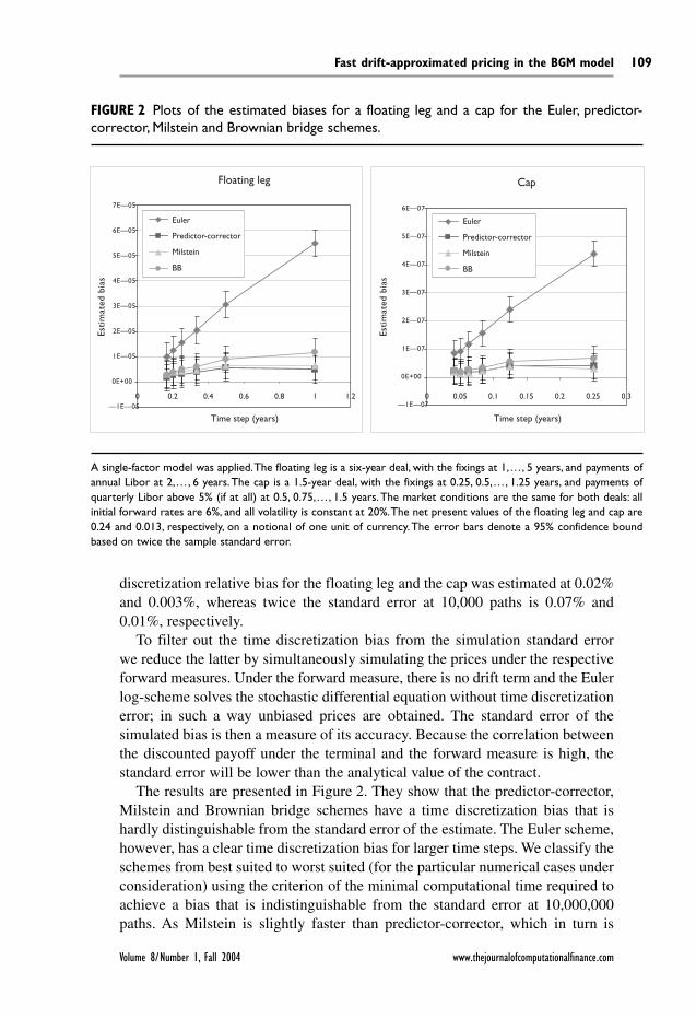
The results are presented in Figure 2. They show that the predictor-corrector,Milstein and Brownian bridge schemes have a time discretization bias that ishardly distinguishable from the standard error of the estimate. The Euler scheme,however, has a clear time discretization bias for larger time steps. We classify theschemes from best suited to worst suited (for the particular numerical cases underconsideration) using the criterion of the minimal computational time required toachieve a bias that is indistinguishable from the standard error at 10,000,000paths. As Milstein is slightly faster than predictor-corrector, which in turn is



109

FIGURE 2 Plots of the estimated biases for a floating leg and a cap for the Euler, predictor-corrector, Milstein and Brownian bridge schemes.

Esti

mat

ed b

ias

Floating leg

Time step (years)

Euler

Predictor-corrector

Milstein

BB

Time step (years)

Esti

mat

ed b

ias

Cap

Euler

Predictor-corrector

Milstein

BB

6E—07

5E—07

4E—07

3E—07

2E—07

1E—07

0E+00

—1E—070 0.05 0.1 0.15 0.2 0.25 0.30 0.2 0.4 0.6 0.8 1 1.2

7E—05

6E—05

5E—05

4E—05

3E—05

2E—05

1E—05

0E+00

—1E—05

A single-factor model was applied.The floating leg is a six-year deal, with the fixings at 1,…, 5 years, and payments ofannual Libor at 2,…, 6 years.The cap is a 1.5-year deal, with the fixings at 0.25, 0.5,…, 1.25 years, and payments ofquarterly Libor above 5% (if at all) at 0.5, 0.75,…, 1.5 years.The market conditions are the same for both deals: allinitial forward rates are 6%, and all volatility is constant at 20%.The net present values of the floating leg and cap are0.24 and 0.013, respectively, on a notional of one unit of currency.The error bars denote a 95% confidence boundbased on twice the sample standard error.

faster than the Brownian bridge, we obtain: first, Milstein; second, predictor-corrector; third, Brownian bridge; and fourth, Euler. We stress here that this clas-sification might be particular to the numerical cases that we considered. We alsostress that the strength of the Brownian bridge lies in single time steps rather thanin multi-time steps.

6 Example: one-factor drift-approximated BGM framework

This section illustrates the framework for fast single time step pricing in BGM bysetting it up in the special case of a one-factor model with a volatility structure asin the example in Section 3.3. This structure may be written as follows:

σi(t) = γi eκ t

for certain constants γi. The corresponding Markov factor, X, is then defined asand characterized by

X(t) N (0, Σ2(t))

where

Prices may now be computed by either numerical integration or finite differences.In the case of numerical integration, if Π(t, X ) denotes the numeraire-deflatedvalue of the contingent claim, we have

where t denotes the expiry of the contingent claim and p( · ; µ, Σ2) denotes theGaussian density with mean µ and standard deviation Σ. In case of finite differ-ences, Feynman–Kac yields the following PDE for the price relative to theterminal bond:

(21)

with use of appropriate boundary conditions. For example, for a Bermudan payerswaption we have Π( · , –∞) ≡ 0, zero convexity ∂2Π ⁄ ∂X2 ≡ 0 at X = ∞, andexercise boundary conditions at the exercise times.

∂

∂+

∂

∂=

Π Π

t Xt

1

202

2

2e κ

Π Π Σ0 0 0 2, ( ) ( , ) ; , ( )X t x p x t x( ) = ( )− ∞

∞

∫ d

Σ2 2

0

2 1

20

0

( ),

,

t sk

t k

s

tt

= =−

≠

=

∫ e de

κ

κ

κ

X t W ss

t

( ) ( ),= ∫ e dκ

0



110

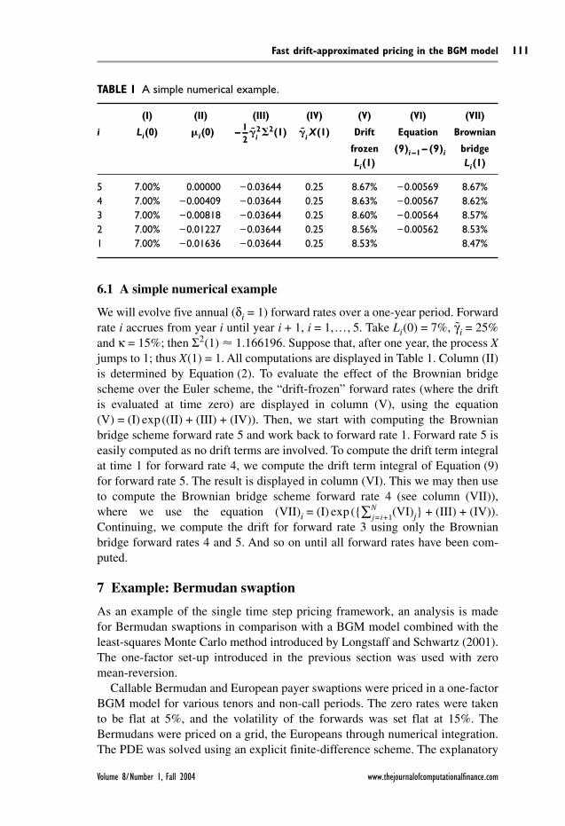
6.1 A simple numerical example

We will evolve five annual (δi = 1) forward rates over a one-year period. Forwardrate i accrues from year i until year i + 1, i = 1,…, 5. Take Li(0) = 7%, γi = 25%and κ = 15%; then Σ2(1) 1.166196. Suppose that, after one year, the process Xjumps to 1; thus X(1) = 1. All computations are displayed in Table 1. Column (II)is determined by Equation (2). To evaluate the effect of the Brownian bridgescheme over the Euler scheme, the “drift-frozen” forward rates (where the driftis evaluated at time zero) are displayed in column (V), using the equation(V) = (I) exp ((II) + (III) + (IV)). Then, we start with computing the Brownianbridge scheme forward rate 5 and work back to forward rate 1. Forward rate 5 iseasily computed as no drift terms are involved. To compute the drift term integralat time 1 for forward rate 4, we compute the drift term integral of Equation (9)for forward rate 5. The result is displayed in column (VI). This we may then useto compute the Brownian bridge scheme forward rate 4 (see column (VII)),where we use the equation (VII)i = (I) exp (∑N

j= i+1(VI)j + (III) + (IV)).Continuing, we compute the drift for forward rate 3 using only the Brownianbridge forward rates 4 and 5. And so on until all forward rates have been com-puted.

7 Example: Bermudan swaption

As an example of the single time step pricing framework, an analysis is madefor Bermudan swaptions in comparison with a BGM model combined with theleast-squares Monte Carlo method introduced by Longstaff and Schwartz (2001).The one-factor set-up introduced in the previous section was used with zeromean-reversion.

Callable Bermudan and European payer swaptions were priced in a one-factorBGM model for various tenors and non-call periods. The zero rates were takento be flat at 5%, and the volatility of the forwards was set flat at 15%. TheBermudans were priced on a grid, the Europeans through numerical integration.The PDE was solved using an explicit finite-difference scheme. The explanatory



111

TABLE 1 A simple numerical example.

(I) (II) (III) (IV) (V) (VI) (VII)

i Li(0) i(0) – 1–2

i22(1) i X(1) Drift Equation Brownian

frozen (9)i –1 – (9)i bridgeLi(1) Li(1)

5 7.00% 0.00000 –0.03644 0.25 8.67% –0.00569 8.67%4 7.00% –0.00409 –0.03644 0.25 8.63% –0.00567 8.62%3 7.00% –0.00818 –0.03644 0.25 8.60% –0.00564 8.57%2 7.00% –0.01227 –0.03644 0.25 8.56% –0.00562 8.53%1 7.00% –0.01636 –0.03644 0.25 8.53% 8.47%

variable in the least-squares Monte Carlo was taken to be the NPV of the under-lying swap. This was regressed on to a constant and a linear term. These two basisfunctions yield sufficiently accurate results because the value of a Bermudanswaption increases almost linearly with the value of the underlying swap.

Problems may possibly occur for American-style derivatives in the single timestep framework. Since the framework is not arbitrage-free, spurious early ordelayed exercise may take place to collect the arbitrage opportunity. The effectsof these phenomena have been analyzed by comparing the exercise boundaries3

and risk sensitivities of Longstaff–Schwartz and single time step BGM. In both



112

TABLE 2 Specification of the Bermudan swaption comparison deal.

Callable Bermudan swaptionMarket dataZero rates Flat at 5%Volatility Flat at 15%

Product specificationTenor Variable (2–8 years)Non-call period VariableCall dates Semi-annualPay/receive Pay fixed

Fixed leg propertiesFrequency Semi-annualDate roll NoneDay count Half year = 0.5Fixed rate 5.06978% (ATM)

Floating leg propertiesFrequency Semi-annualDate roll NoneDay count Half year = 0.5Margin 0%

NumericsSimulation paths 10,000Finite-difference scheme Explicit

Longstaff–SchwartzExplanatory variable Swap NPVBasis function type MonomialsNo. of basis functions Two (constant and linear)

3 In the Longstaff–Schwartz case, the future discounted cashflows are regressed against theNPV of the underlying swap with a constant and linear term – say, with coefficients a and b.So the option is exercised whenever S > a + bS ⇔ S > a(1 – b) =: S*, where it is assumedthat b < 1, which turns out to hold in practice. Hence the exercise boundary S* may be com-puted from the regression coefficients by the above formula.

models the exercise rule turned out to be of the following form: exercise when-ever the NPV of the underlying swap, S, is larger than a certain value S*, whichis then defined to be the exercise boundary.

For a full description of the deal see Table 2. Results have been summarizedin Table 3. Computational times may be found in Table 4. Exercise boundariesfor the 8 year deal are displayed in Figure 3, including confidence bounds on theLongstaff–Schwartz boundaries.4 We looked at exercise boundaries for other deals



113

4 The empirical covariance matrix of the regression-estimated coefficients a and b may beused to obtain the empirical variance of S*. Denote random errors in a and b by a and b,respectively. If it is assumed that these errors are relatively small, a Taylor expansion yields(ignoring second-order terms)

We thus obtain the empirical variance of S* (as well as its standard error). Assuming that S* is nor-mally distributed, a 95% confidence interval is given by plus and minus twice the standard error.

Sa

b a b

a b* ≈−

+ +−

11

1

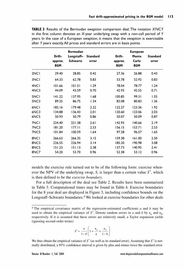
TABLE 3 Results of the Bermudan swaption comparison deal. The notation XNCYin the first column denotes an X-year underlying swap with a non-call period of Yyears. In the case of a European swaption, it means that the swaption is exercisableafter Y years exactly.All prices and standard errors are in basis points.

Bermudan EuropeanDrift- Longstaff– Standard Drift- Monte Standard

approx. Schwartz error approx. Carlo errorBGM BGM BGM

2NC1 29.40 28.85 0.42 27.36 26.88 0.43

3NC1 64.33 62.78 0.83 53.78 52.92 0.83

4NC1 101.66 101.51 1.29 78.04 78.77 1.244NC3 44.09 43.59 0.70 42.93 42.55 0.71

5NC1 141.22 137.95 1.68 100.85 99.31 1.555NC3 89.25 86.75 1.34 83.08 80.83 1.36

6NC1 182.16 179.48 2.22 122.27 123.36 1.926NC3 134.88 136.43 2.01 120.60 123.06 2.036NC5 50.93 50.79 0.86 50.07 50.09 0.87

7NC1 224.40 221.38 2.61 142.93 140.66 2.197NC3 181.20 177.11 2.53 156.15 153.71 2.537NC5 101.84 100.59 1.64 97.28 96.57 1.65

8NC1 266.63 266.35 3.15 159.38 161.00 2.508NC3 226.55 226.94 3.14 185.20 190.98 3.088NC5 151.23 151.13 2.38 137.73 140.95 2.418NC7 54.20 53.70 0.96 52.38 53.12 0.96



114

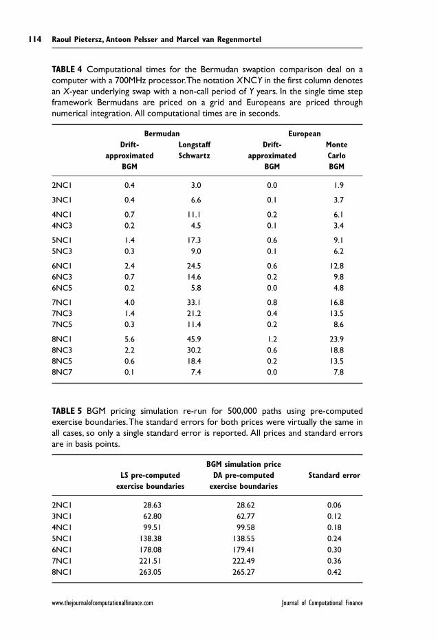
TABLE 4 Computational times for the Bermudan swaption comparison deal on acomputer with a 700MHz processor.The notation XNCY in the first column denotesan X-year underlying swap with a non-call period of Y years. In the single time stepframework Bermudans are priced on a grid and Europeans are priced throughnumerical integration. All computational times are in seconds.

Bermudan EuropeanDrift- Longstaff Drift- Monte

approximated Schwartz approximated CarloBGM BGM BGM

2NC1 0.4 3.0 0.0 1.9

3NC1 0.4 6.6 0.1 3.7

4NC1 0.7 11.1 0.2 6.14NC3 0.2 4.5 0.1 3.4

5NC1 1.4 17.3 0.6 9.15NC3 0.3 9.0 0.1 6.2

6NC1 2.4 24.5 0.6 12.86NC3 0.7 14.6 0.2 9.86NC5 0.2 5.8 0.0 4.8

7NC1 4.0 33.1 0.8 16.87NC3 1.4 21.2 0.4 13.57NC5 0.3 11.4 0.2 8.6

8NC1 5.6 45.9 1.2 23.98NC3 2.2 30.2 0.6 18.88NC5 0.6 18.4 0.2 13.58NC7 0.1 7.4 0.0 7.8

TABLE 5 BGM pricing simulation re-run for 500,000 paths using pre-computedexercise boundaries.The standard errors for both prices were virtually the same inall cases, so only a single standard error is reported. All prices and standard errorsare in basis points.

BGM simulation priceLS pre-computed DA pre-computed Standard error

exercise boundaries exercise boundaries

2NC1 28.63 28.62 0.063NC1 62.80 62.77 0.124NC1 99.51 99.58 0.185NC1 138.38 138.55 0.246NC1 178.08 179.41 0.307NC1 221.51 222.49 0.368NC1 263.05 265.27 0.42

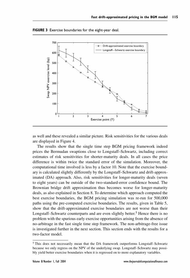
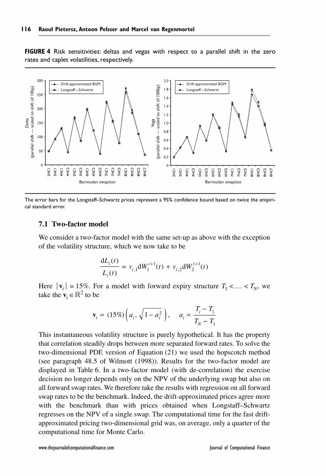
as well and these revealed a similar picture. Risk sensitivities for the various dealsare displayed in Figure 4.

The results show that the single time step BGM pricing framework indeedprices the Bermudan swaptions close to Longstaff–Schwartz, including correctestimates of risk sensitivities for shorter-maturity deals. In all cases the pricedifference is within twice the standard error of the simulation. Moreover, thecomputational time involved is less by a factor 10. Note that the exercise bound-ary is calculated slightly differently by the Longstaff–Schwartz and drift-approx-imated (DA) approach. Also, risk sensitivities for longer-maturity deals (sevento eight years) can be outside of the two-standard-error confidence bound. TheBrownian bridge drift approximation thus becomes worse for longer-maturitydeals, as also explained in Section 8. To determine which approach computed thebest exercise boundaries, the BGM pricing simulation was re-run for 500,000paths using the pre-computed exercise boundaries. The results, given in Table 5,show that the drift-approximated exercise boundaries are not worse than theirLongstaff–Schwartz counterparts and are even slightly better.5 Hence there is noproblem with the spurious early exercise opportunities arising from the absence ofno-arbitrage in the fast single time step framework. The non-arbitrage-free issueis investigated further in the next section. This section ends with the results for atwo-factor model.



115

5 This does not necessarily mean that the DA framework outperforms Longstaff–Schwartzbecause we only regress on the NPV of the underlying swap. Longstaff–Schwartz may possi-bly yield better exercise boundaries when it is regressed on to more explanatory variables.

FIGURE 3 Exercise boundaries for the eight-year deal.

1 2 3 4 5 6 70

100

200

300

400

500

600

700

Exercise point (Y )

Swap

NPV

exe

rcis

e le

vel (

bp)

Drift-approximated exercise boundary

Longstaff—Schwartz exercise boundary

7.1 Two-factor model

We consider a two-factor model with the same set-up as above with the exceptionof the volatility structure, which we now take to be

Here vi = 15%. For a model with forward expiry structure T1 < … < TN, wetake the vi ∈2 to be

This instantaneous volatility structure is purely hypothetical. It has the propertythat correlation steadily drops between more separated forward rates. To solve thetwo-dimensional PDE version of Equation (21) we used the hopscotch method(see paragraph 48.5 of Wilmott (1998)). Results for the two-factor model aredisplayed in Table 6. In a two-factor model (with de-correlation) the exercisedecision no longer depends only on the NPV of the underlying swap but also onall forward swap rates. We therefore take the results with regression on all forwardswap rates to be the benchmark. Indeed, the drift-approximated prices agree morewith the benchmark than with prices obtained when Longstaff–Schwartzregresses on the NPV of a single swap. The computational time for the fast drift-approximated pricing two-dimensional grid was, on average, only a quarter of thecomputational time for Monte Carlo.

vi i i ii

N

a a aT T

T T= −( ) =

−

−( %) , ,15 1 2 1

1

dd d

L t

L tv W t v W ti

ii

ii

i( )

( )( ) ( ), ,= ++ +

1 11

2 21



116

FIGURE 4 Risk sensitivities: deltas and vegas with respect to a parallel shift in the zerorates and caplet volatilities, respectively.

2NC

1

3NC

1

4NC

1

4NC

3

5NC

1

5NC

3

6NC

1

6NC

3

6NC

5

7NC

1

7NC

3

7NC

5

8NC

1

8NC

3

8NC

5

8NC

7

2NC

1

3NC

1

4NC

1

4NC

3

5NC

1

5NC

3

6NC

1

6NC

3

6NC

5

7NC

1

7NC

3

7NC

5

8NC

1

8NC

3

8NC

5

8NC

7

Del

ta(p

aral

lel s

hift

— s

cale

d to

shi

ft o

f 10b

p)

Bermudan swaption

300

250

200

150

100

50

0

Vega

(par

alle

l shi

ft —

sca

led

to s

hift

of 1

00bp

)Drift-approximated BGM

Longstaff—Schwartz

2.0

1.8

1.6

1.4

1.2

1.0

0.8

0.6

0.4

0.2

0

Bermudan swaption

Drift-approximated BGM

Longstaff—Schwartz

The error bars for the Longstaff–Schwartz prices represent a 95% confidence bound based on twice the empiri-cal standard error.

8 Test of accuracy of drift approximation

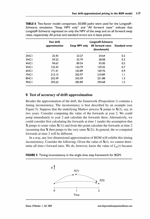
Besides the approximation of the drift, the framework (Proposition 1) contains atiming inconsistency. The inconsistency is best described by an example (seeFigure 5). Suppose that the underlying Markov process X jumps to X(2), say, intwo years. Consider computing the value of the forwards at year 2. We couldjump immediately to year 2 and calculate the forwards there. Alternatively, wecould consider first calculating the forwards at time 1 (under the assumption thatX jumps to some value X(1)) and from this point calculate the forwards at time 2(assuming that X then jumps to the very same X(2)). In general, the so computedforwards at time 2 will be different.

In a way, any low-dimensional approximation of BGM will exhibit this timinginconsistency. Consider the following. Given the value of X(t), we cannot deter-mine all time-t forward rates. We do, however, know the value of LN(t) because



117

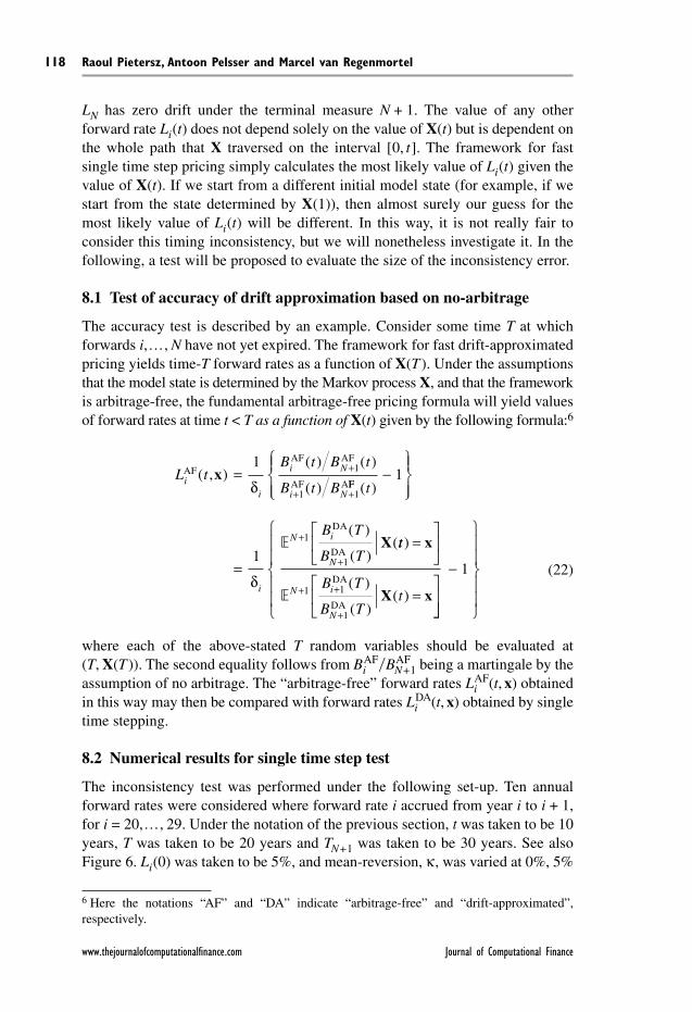
TABLE 6 Two-factor model comparison. 50,000 paths were used for the Longstaff–Schwartz simulation. “Swap NPV only” and “All forward rates” indicate thatLongstaff–Schwartz regressed on only the NPV of the swap and on all forward swaprates, respectively. All prices and standard errors are in basis points.

Fast drift Longstaff–Schwartzapproximation Swap NPV only All forward rates Standard error

(benchmark)

2NC1 25.45 23.27 24.64 0.23NC1 59.22 55.79 58.08 0.34NC1 94.67 89.54 93.00 0.55NC1 132.35 124.79 129.42 0.76NC1 171.41 162.89 169.76 0.97NC1 212.15 202.97 210.89 1.18NC1 252.49 242.59 251.88 1.39NC1 292.62 283.89 294.68 1.5

FIGURE 5 Timing inconsistency in the single time step framework for BGM.

XX(1)

X(2)

0 1 2

Time

LN has zero drift under the terminal measure N + 1. The value of any otherforward rate Li(t) does not depend solely on the value of X(t) but is dependent onthe whole path that X traversed on the interval [0, t]. The framework for fastsingle time step pricing simply calculates the most likely value of Li(t) given thevalue of X(t). If we start from a different initial model state (for example, if westart from the state determined by X(1)), then almost surely our guess for themost likely value of Li(t) will be different. In this way, it is not really fair toconsider this timing inconsistency, but we will nonetheless investigate it. In thefollowing, a test will be proposed to evaluate the size of the inconsistency error.

8.1 Test of accuracy of drift approximation based on no-arbitrage

The accuracy test is described by an example. Consider some time T at whichforwards i,…, N have not yet expired. The framework for fast drift-approximatedpricing yields time-T forward rates as a function of X(T ). Under the assumptionsthat the model state is determined by the Markov process X, and that the frameworkis arbitrage-free, the fundamental arbitrage-free pricing formula will yield valuesof forward rates at time t < T as a function of X(t) given by the following formula:6

(22)

where each of the above-stated T random variables should be evaluated at(T, X(T )). The second equality follows from Bi

AFBAFN+1 being a martingale by the

assumption of no arbitrage. The “arbitrage-free” forward rates LiAF(t, x) obtained

in this way may then be compared with forward rates LiDA(t, x) obtained by single

time stepping.

8.2 Numerical results for single time step test

The inconsistency test was performed under the following set-up. Ten annualforward rates were considered where forward rate i accrued from year i to i + 1,for i = 20,…, 29. Under the notation of the previous section, t was taken to be 10years, T was taken to be 20 years and TN+1 was taken to be 30 years. See alsoFigure 6. Li(0) was taken to be 5%, and mean-reversion, κ, was varied at 0%, 5%

L tB t B t

B t Bi

i

i N

i N

AFAF AF

AF A( , )

( ) ( )

( )x = +

+ +

1 1

1 1δ FF

DA

DA

( )

( )

( )(

t

B T

B T

i

N i

N

−

=

+

+

1

11

1

δ

X tt

B T

B TtN i

N

)

( )

( )( )

=

=

+ +

+

x

X x 1 1

1

DA

DA

−

1



118

6 Here the notations “AF” and “DA” indicate “arbitrage-free” and “drift-approximated”,respectively.

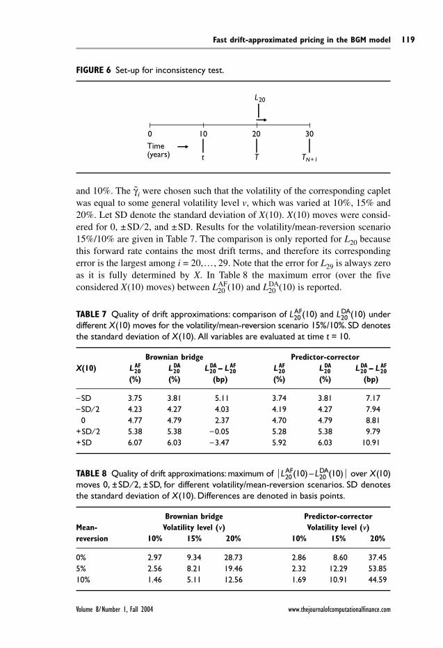
and 10%. The γi were chosen such that the volatility of the corresponding capletwas equal to some general volatility level v, which was varied at 10%, 15% and20%. Let SD denote the standard deviation of X(10). X(10) moves were consid-ered for 0, ±SD ⁄ 2, and ±SD. Results for the volatility/mean-reversion scenario15%/10% are given in Table 7. The comparison is only reported for L20 becausethis forward rate contains the most drift terms, and therefore its correspondingerror is the largest among i = 20,…, 29. Note that the error for L29 is always zeroas it is fully determined by X. In Table 8 the maximum error (over the fiveconsidered X(10) moves) between L20

AF(10) and L20DA(10) is reported.



119

FIGURE 6 Set-up for inconsistency test.

0 10 20 30

L20

Time(years) t T TN+1

TABLE 7 Quality of drift approximations: comparison of L20AF(10) and L20

DA(10) underdifferent X(10) moves for the volatility/mean-reversion scenario 15%/10%. SD denotesthe standard deviation of X(10). All variables are evaluated at time t = 10.

Brownian bridge Predictor-correctorX(10) L20

AF L20DA L20

DA – L20AF L20

AF L20DA L20

DA – L20AF

(%) (%) (bp) (%) (%) (bp)

–SD 3.75 3.81 5.11 3.74 3.81 7.17–SD ⁄ 2 4.23 4.27 4.03 4.19 4.27 7.94

0 4.77 4.79 2.37 4.70 4.79 8.81+SD ⁄ 2 5.38 5.38 –0.05 5.28 5.38 9.79+SD 6.07 6.03 –3.47 5.92 6.03 10.91

TABLE 8 Quality of drift approximations: maximum of L20AF(10) – L20

DA(10) over X(10)moves 0, ±SD ⁄ 2, ±SD, for different volatility/mean-reversion scenarios. SD denotesthe standard deviation of X(10). Differences are denoted in basis points.

Brownian bridge Predictor-correctorMean- Volatility level (v) Volatility level (v)reversion 10% 15% 20% 10% 15% 20%

0% 2.97 9.34 28.73 2.86 8.60 37.455% 2.56 8.21 19.46 2.32 12.29 53.8510% 1.46 5.11 12.56 1.69 10.91 44.59

The test was performed for both the Brownian bridge and predictor-correctorschemes. The results show that the former outperforms the latter in the timinginconsistency test.

The inconsistency test results show that, for less volatile market scenarios, thesingle time step framework performs very accurately, with errors only up to a fewbasis points. For more volatile market scenarios the approximation deteriorates.But for realistic yield curve and forward volatility scenarios there are no prob-lems with respect to pricing (see Section 7). The worsening of the approximationfor more volatile scenarios is what may be expected from the nature of the driftapproximations: as the model dimensions increase, the single time step approxi-mation will break up. By “model dimensions” we mean the volatility level, thetenor of the deal, the difference between the forward index i and N, or time zeroforward rates, etc. Care should be taken in applying the single time step frame-work for BGM that the market scenario does not violate the realm where thesingle time step approximation is reasonably valid.

9 Conclusions

We have introduced a fast approximate pricing framework as an addition to thepredictor-corrector drift approximation developed by Hunter, Jäckel and Joshi(2001a). These authors used the drift approximation only to speed up their MonteCarlo by reducing it to single time step simulation. We have shown that, at aslight cost, much faster computational methods may be used, such as numericalintegration or finite differences. The additional cost is a non-restrictive assump-tion, namely, separability of the volatility function. The proposed drift approxi-mation framework was applied to the pricing of Bermudan swaptions, for whichit yielded very accurate prices with much lower computation times.

Appendix A Mean of generalized geometric Brownian bridge

In this appendix, the time-t mean of the process Lk defined in Equation (9) isdetermined. Equivalently, we may determine the time-t mean of the process Y,given by

(Compare with Equation (9).) The solution of Y (unconditional of time-t*) isgiven by

Y t yX t t

( )( ) ( )

=−

0

1

22

eΣ

dd

Y t

Y tt t Y y Y t

( )

( )( ) ( ) , ( ) , ( )*= ⋅ = =σ W 0 0 yy*



120

where

Note that

ω ∈Ω; Y(t*) = y* = ω ∈Ω; X(t*) = log (y*y0) + 1–2

Σ2(t*) =: x*According to the martingale time change theorem (for example Theorem 4.6 ofKaratzas and Shreve (1991)), we have that X(τ( · )) is a Brownian motion, wherethe time change τ is defined by

τ (t) = infs ≥ 0; Σ2(t) > s

Working in the time-changed time coordinates, X( · )X(τ*) = x* is a standardBrownian bridge, and so, according to Section 5.6.B of Karatzas and Shreve(1991),

X(τ )X(τ*) = x* N

Back in the original time coordinates, this translates to

X(t)X(t*) = x* N

With this, we may evaluate the mean of Y(t)Y(t*) = y* to be

where the following simple rule has been used: [eZ] = eβ+τ2 ⁄ 2 whenever Z isnormally distributed, Z N (β, τ2).

Appendix B Approximation of substituting the mean in theexpectation of expression (9)

In Section 3 a four-step method for the calculation of expression (9) is described.An approximating fourth step is proposed that evaluates the expectation ofthe BGM drift inserting the mean. In this appendix an error bound for thisapproximation is derived, and it is shown that the approximation is of order twoin volatility in the neighbourhood of zero.

Y t Y t y yy

y

t

T

( ) ( ) exp* **

( )

( )

=[ ] =

0

0

2

2 1

2

Σ

Σ ΣΣ

ΣΣ Σ

2

22 2

( )

( )( ) ( )

t

TT t−( )

t

tx t

t( )

( ), ( )

( )

** −

( )Σ

ΣΣ

Σ

Σ

2

22

2 2

22( )*t

x ,*

**

τ

ττ

τ

τ−

2

X t s s t s st t

( ) : ( ) ( ), ( ) : ( )= ⋅ =∫ ∫σ σd dW0

2 2

0

Σ



121

The expectation term can always be rewritten as

where Z is distributed standard normally. It is straightforward to verify that theabove function f : 2 → is infinitely differentiable at every point of the wholereal plane. Note that approximating the above expectation at the mean signifiesthat the above function is approximated as

Fix µ and calculate the derivative of f with respect to σ. The interchange of dif-ferentiation and expectation is a subtle argument that may, for example, be foundin Williams (1991, paragraph A.16.1). We carefully verified that in the above caseall the requirements for interchange are satisfied. We then find

Due to the odd nature of the above integrand at the point σ = 0, we find that

Taylor’s formula then states that there exists C ≥ 0 (possibly depending on µ)such that

Because a bound on the second derivative of σ f (µ, σ) may be found inde-pendently of µ on some interval [0, σ– ], it follows from Theorem 7.7 of Apostol(1967) that the constant C may then be chosen independently of µ for allσ ∈[0, σ– ].

f C( , )exp

exp µ σ

µ

µσ−

+≤

12

∂∂

=f

σµ( , )0 0

∂∂

=+

+ +( )

fZ

Z

Zσµ σ

µ σ

µ σ( , )

exp

exp

12

f f( , ) ( , )exp

exp µ σ µ

µ

µ≈ =

+0

1

fZ

Z( , )

exp

exp µ σ

µ σµ σ

=+

+ +

1



122

REFERENCES

Apostol, T. M. (1967). Calculus, Volume 1, Second edition. John Wiley & Sons, Chichester.

Avramidis, A. N., and Matzinger, H. (2004). Convergence of the stochastic mesh estimator forpricing Bermudan options. Journal of Computational Finance 7(4), 73–91.

Björk, T., Landén, C., and Svensson, L. (2002). Finite dimensional Markovian realizations forstochastic volatility forward rate models. Working paper.

Brace, A., Gatarek, D., and Musiela, M. (1997). The market model of interest rate dynamics.Mathematical Finance 7(2), 127–55.

Brigo, D., and Mercurio, F. (2001). Interest rate models: theory and practice. Springer-Verlag,Berlin.

Broadie, M., and Glasserman, P. (1996). Estimating security price derivatives using simulation.Management Science 42(2), 269–85.

Broadie, M., and Glasserman, P. (2004). A stochastic mesh method for pricing high-dimen-sional American options. Journal of Computational Finance 7(4), 35–72.

De Jong, F., Driessen, J., and Pelsser, A. A. J. (2002). LIBOR market models versus swap mar-ket models for pricing of interest rate derivatives: an empirical analysis. European FinanceReview 5(3), 201–37.

Glasserman, P., and Merener, N. (2003a). Cap and swaption approximations in LIBOR marketmodels with jumps. Journal of Computational Finance 7(1), 1–36.

Glasserman, P., and Merener, N. (2003b). Numerical solution of jump–diffusion LIBORmarket models. Finance and Stochastics 7(1), 1–27.

Glasserman, P., and Merener, N. (2004). Convergence of a discretization scheme for jump–

diffusion processes with state-dependent intensities. Proceedings of the Royal Society460(2041), 111–27.

Glasserman, P., and Zhao, X. (1999). Fast Greeks by simulation in forward LIBOR models.Journal of Computational Finance 3(1), 5–39.

Heath, D., Jarrow, R., and Morton, A. (1992). Bond pricing and the term structure of interestrates: a new methodology for contingent claims valuation. Econometrica 60(1), 77–105.

Hughston, L. P., and Rafailidis, A. (2002). A chaotic approach to interest rate modelling. Toappear in Finance and Stochastics.

Hunt, P., Kennedy, J., and Pelsser, A. A. J. (2000). Markov-functional interest rate models.Finance and Stochastics 4(4), 391–408.

Hunter, C. J., Jäckel, P., and Joshi, M. S. (2001a). Drift approximations in a forward-rate-basedLIBOR market model. Working paper, www.rebonato.com.

Hunter, C. J., Jäckel, P., and Joshi, M. S. (2001b). Getting the drift. Risk, July.

Jäckel, P. (2002). Monte Carlo methods in finance. J. Wiley & Sons, Chichester.

Jamshidian, F. (1996). LIBOR and swap market models and measures. Working paper, SakuraGlobal Capital, London.

Jamshidian, F. (1997). LIBOR and swap market models and measures. Finance andStochastics 1(4), 293–330.



123

Karatzas, I., and Shreve, S. E. (1991). Brownian motion and stochastic calculus, Secondedition. Springer-Verlag, Berlin.

Kloeden, P. E., and Platen, E. (1999). Numerical solution of stochastic differential equations,Volume 23 of Applications of mathematics. Springer-Verlag, Berlin.

Kurbanmuradov, O., Sabelfeld, K., and Schoenmakers, J. (1999). Lognormal random fieldapproximations to LIBOR market models. Working paper, Weierstrass Institute, Berlin(www.wias-berlin.de).

Kurbanmuradov, O., Sabelfeld, K., and Schoenmakers, J. (2002). Lognormal approximationsto LIBOR market models. Journal of Computational Finance 6(1), 69–100.

Longstaff, F. A., and Schwartz, E. S. (2001). American options by simulation: a simple least-squares approach. Review of Financial Studies 14(1), 113–47.

Miltersen, K. R., Sandmann, K., and Sondermann, D. (1997). Closed form solutions for termstructure derivatives with log-normal interest rates. Journal of Finance 52(1), 409–30.

Musiela, M., and Rutkowski, M. (1997). Continuous-time term structure models: forwardmeasure approach. Finance and Stochastics 1(4), 261–91.

Pelsser, A. A. J. (2000). Efficient methods for valuing interest rate derivatives. Springer-Verlag,Berlin.

Ritchken, P., and Sankarasubramanian, L. (1995). Volatility structures of the forward rates andthe dynamics of the term structure. Mathematical Finance 5(1), 55–72.

Williams, D. (1991). Probability with martingales. Cambridge University Press, Cambridge.

Wilmott, P. (1998). Derivatives: the theory and practice of financial engineering. John Wiley& Sons, Chichester.



124

Documents

Fast drift-approximated pricing in the BGM model Notation for BGM model In this section our notation of the BGM model is introduced. Consider a BGM model,M.1 Such a model features