A belief-based theory of homophily∗

Willemien Kets† Alvaro Sandroni‡

March 4, 2015

Abstract

We introduce a model of homophily that does not rely on the assumption of ho-

mophilous preferences. Rather, it builds on the dual process account of Theory of Mind

in psychology which focuses on the role of introspection in decision making. Homophily

emerges because players find it easier to put themselves in each other’s shoes when they

share a similar background. The model delivers novel comparative statics that emphasize

the interplay of cultural and economic factors. Whether homophily is socially optimal

depends crucially on the degree of economic stability.

∗We thank Sandeep Baliga, Vincent Crawford, Georgy Egorov, Tim Feddersen, Matthew Jackson, Rachel

Kranton, Nicola Persico, Yuval Salant, Paola Sapienza, Rajiv Sethi, Eran Shmaya, Andy Skrzypacz, Jakub

Steiner, Jeroen Swinkels, and numerous seminar audiences and conference participants for helpful comments

and stimulating discussions. Alex Limonov provided research assistance.†Kellogg School of Management, Northwestern University. E-mail: w-kets@kellogg.northwestern.edu‡Kellogg School of Management, Northwestern University. E-mail: sandroni@kellogg.northwestern.edu

1

1. Introduction

Homophily, the tendency of people to interact with similar people, is a widespread phe-

nomenon that has been studied in a variety of different fields, ranging from economics (Ben-

habib et al., 2010), to organizational research (Borgatti and Foster, 2003), social psychology

(Gruenfeld and Tiedens, 2010), political science (Mutz, 2002), and sociology (McPherson et al.,

2001). Homophily produces segregated social and professional networks, affect hiring and pro-

motion decisions, investment in education, and the diffusion of information. For decades,

these matters have been at the center of political confrontations and public policy. Thus,

understanding the root sources of homophily is of paramount importance.

Much of the existing literature explains homophily by assuming a direct preference for

associating with similar others (see Jackson, 2014, for a survey). However, without a theory

of the determinants of these preferences, it is difficult to explain why homophily is observed

in some cases, but not in others (beyond positing homophilous preferences only in the former

cases). We provide a theory of homophily that does not assume homophilous preferences.

Rather, these preferences are a natural outcome of individuals’ desire to reduce uncertainty in

strategic settings. Our framework makes it possible to evaluate different policy interventions

and to derive clear and intuitive comparative statics.

Our starting point is that to understand homophily we need to unlook the black box of

cultural identity. Following Kreps (1990), we view culture as a means to reduce strategic

uncertainty. To fix ideas, consider a manager and an employee. The manager can choose a

direct or indirect communication style, and the employee can choose a mode of interpretation.

While direct communication is appropriate in some settings, sometimes tact is called for.

When there is uncertainty about the appropriate behavior, cultural rules can act as focal

principles. If the manager and employee have a similar background, they will typically agree

on what mode of communication is appropriate in a given context, and they will be able to

communicate effectively.

As a metaphor for situations that are characterized by strategic uncertainty, we consider

(pure) coordination games like the following:

s1 s2

s1 1,1 0,0

s2 0,0 1,1

Such games are rife with strategic uncertainty: the payoff structure provides little guidance for

action. However, there may be a focal point in this game, which may depend on the context

of the game. If players share a cultural code, they may successfully coordinate by inferring

the same focal point from the context of the game.

2

To formally model these ideas and connect them to the problem of homophily, we build

on the dual process account of Theory of Mind in psychology.1 The dual process account of

Theory of Mind posits that an individual start with instinctive reactions and then adapt his

views by reasoning about what he would do if he were in the opponent’s position. To capture

this, we assume that each player has some initial (random) impulse telling him which action

is appropriate. A player’s first reaction is to follow his impulse. By introspection, the player

realizes that he may act on instinct and so, his opponent may also act on instinct. In addition,

he reasons that if his opponent is similar to him that the impulse of the opponent may also

be similar to his own. This means that impulses can be used as input to form initial beliefs.

But if the player thinks a little more, he realizes that his opponent may have gone through a

similar reasoning process, leading the player to revise his initial beliefs. This process continues

to higher orders. The limit of this procedure, where players go through the entire reasoning

process in their mind before making a decision, defines an introspective equilibrium.

In line with neurological and behavioral evidence (de Vignemont and Singer, 2006; Jackson

and Xing, 2014), players find it easier to put themselves into the shoes of players that are similar

to them.2 Formally, players belong to different groups, and initial impulses are (imperfectly)

correlated within groups and independent across groups. So, players from the same group are

more likely to agree on which action is focal.

Our first result shows that there is an unique introspective equilibrium, and in this equi-

librium each player follows his initial impulse. So, the naive response of following one’s initial

impulse is, in fact, optimal under the infinite process of reasoning through higher-order beliefs.

This holds even if impulses are noisy and people from different subcultures have uncorrelated

impulses. It now follows that similar players coordinate more effectively. This provides an

incentive to seek out similar people, that is, to be homophilous.3

One way players can enhance the chance of interacting with each other is to choose the same

project (e.g., a hobby, profession, or neighborhood). So, we consider an extended game where

players first choose a project and subsequently play the coordination game with an opponent

that has chosen the same project. We analyze this extended game using the same method

as before. Players introspect on their impulses, use them to form initial beliefs and finally

1See Epley and Waytz (2010) for a survey. The dual process account of Theory of Mind relies on a rapid

instinctive process and a slower cognitive process. So, it is related to the two-systems account of decision-

making under uncertainty, popularized by Kahneman (2011). The foundations of dual processes theory go

back to the work of the psychologist William James (1890/1983). See Section 2 for an extended discussion.2Empirical and experimental evidence also shows that people trust people that are similar to them more

(DeBruine, 2002; Guiso et al., 2009).3Alternatively, players could reduce the risk of miscoordinating by learning the cultural code of the other

group (Lazear, 1999). However, this may be costly.

3

modify them through higher-order reasoning. We show that there is a unique introspective

equilibrium. In the unique equilibrium, players from the same group overwhelmingly choose

the same project, regardless of their intrinsic sentiments over projects. The level of homophily

depends on economic incentives (i.e., the coordination payoffs) and the strength of cultural

identity (i.e., similarity in impulses within a group). Thus, introspection and reasoning lead

to effective coordination as well as homophily.

Our results show that the root cause of homophily may not be a direct taste for interacting

with similar others, but rather reflects a preference to reduce strategic uncertainty. This

approach is consistent with the observation that homophily is often based on traits that

are behaviorally relevant (e.g., profession, religion) rather than traits that are not directly

tied to behavior, such as height (McPherson et al., 2001). This allows us to explain the

prevalence of homophily in organizational settings, as discussed in Section 1.1. Our model also

allows us to shed light on various empirical regularities, such as why homophily is observed

in some settings, but not in others, even if the underlying game is similar. For example,

some organizational cultures do not strongly guide initial impulses, and this leads to less

segregated networks (Staber, 2001). Consistent with these observations, our model predicts

that the level of homophily is lower when cultural identity is weaker. Finally, regardless of

the distribution over impulses, when coordination payoffs are high, the level of homophily

is necessarily high. This is a testable implication of our model that does easily follow from

standard game-theoretical models.

We next turn to the question of optimal social structure. We allow for uncertainty about

the underlying game. Either the game is the pure coordination game considered above, or

one of the equilibria Pareto dominates the other. We distinguish two cases. The first case

concerns a stable economic environment: with high probability, the game is close to the

pure coordination game. The second case considers an uncertain economic environment where

there is a significant chance that an innovation significantly enhances the payoffs in the Pareto-

dominant equilibrium. We investigate how the social structure that maximizes social welfare

depends on the economic environment.

If the economic environment is stable, it is socially optimal to have high levels of homophily.

Moreover, strengthening players’ cultural identity reduces strategic uncertainty and increases

social welfare, even though it leads to segregation. This may be the purpose of policies

that strengthen cultural identity in organizations (e.g., Tichy and Sherman, 2005) and at the

national level (Macdonald, 2012).

The conclusions are starkly different in an uncertain economic environment. In this case,

social welfare is maximal if there is a minority of a significant size. Intuitively, a member of

the minority group faces less pressure to conform than a member of the majority group. This

4

is because a player from the minority group is unlikely to be matched with a player from his

own group, and thus faces only a weak incentive to conform to the (expected) action choice

by members of his group. He may thus take the high-payoff action even if it goes against his

impulse. To maximize social welfare, this non-conformist behavior of the minority has to spill

over to the majority, so that all players choose the high-payoff action. This can happen only

if the minority has a critical mass. As before, strengthening players’ cultural identity reduces

strategic uncertainty, but the welfare effects are now reversed: social welfare is lower if cultural

identity is stronger. This is because the stronger players’ cultural identity, the stronger the

pressure to conform, and thus the harder it is for players to choose the high-payoff action

when it is against their initial impulse. This suggests a rationale for promoting diversity even

in the absence of complementarity of skills across groups: a more diverse organization harbors

dissent, and dissent may prevent excessive conformism in the face of innovations.

So, whereas a segregated organization with a strong cultural identity does well in a stable

economic environment, the same factors that make such an organization successful at coor-

dination also limits its flexibility when potentially Pareto improving innovations are likely.

By contrast, more integrated organizations with a weaker cultural identity have the agility to

perform well in such an uncertain environment, consistent with historical evidence (Mokyr,

1990). As we discuss in Section 4, these results cannot be obtained using the standard frame-

work. In particular, the standard framework cannot explain how the optimal social structure

depends on the economic environment. Formally modeling a mechanism that can capture

these common intuitions has several benefits. First, it allows us to ask how the optimal size

of the minority varies with primitives such as the strength of players’ cultural identity and

the coordination payoff. Moreover, it allows us to characterize the conditions under which

homophily is socially optimal.

Thus far, we have assumed that all players are matched with exactly one other player.

Section 5 captures network formation, by allowing players to interact with multiple players at

a cost. The level of homophily can now be even higher, as greater success in coordinating with

similar others translates into greater incentives to form connections. In addition, the model

accommodates important properties of social and economic networks. Since these features

arise endogenously, the model provides novel testable hypotheses about how these properties

change when the fundamentals vary. For example, when cultural identity is strong, networks

tend to be densely connected, with high levels of homophily and significant inequality in

the number of connections. This means that the network consists of a tightly connected

core of gregarious players from one group, with a periphery of hermits from the other group

that are loosely connected with the core, consistent with empirical observations of social and

economic networks (Jackson, 2008). Other extensions of the model consider the effects of

5

skill complementarities between groups (Appendix D) and the ability to use markers, such as

tatoos or business attire, as a way to signal cultural identity (Appendix C).

The heart of our contribution lies in the modeling of players’ reasoning process. In a setting

where standard equilibrium refinements have no bite, an explicit model of players’ reasoning

process is a powerful method to obtain uniqueness in a range of different settings.4 This

equilibrium uniqueness permits intuitive yet subtle comparative statics, and allows for direct

welfare analysis of commonly used policies.

1.1. Related literature

Homophily is a widespread phenomenon that has important economic implications, af-

fecting hiring and promotion decisions, the spread of information and educational outcomes

(Jackson, 2014). The literature on homophily in economics mostly assumes homophilous pref-

erences and investigates the implications for network structure and economic outcomes (e.g.,

Schelling, 1971; Alesina and La Ferrara, 2000; Currarini et al., 2009; Golub and Jackson, 2012;

Alger and Weibull, 2013), with Baccara and Yariv (2013) and Peski (2008) being notable ex-

ceptions.5 By contrast, we derive players’ incentives to interact with similar others from a

desire to reduce strategic uncertainty. This makes it possible to obtain intuitive comparative

statics and to evaluate the tradeoffs inherent in diversity policies.

Our approach is particularly well-suited to study the prevalence of homophily in organi-

zational settings (McPherson et al., 2001). Consistent with our approach, homogenous teams

tend to have fewer coordination and communication problems, and teams and organizations

tend to be homophilous as a result (Brass et al., 2004; Jackson et al., 2003; Milliken and Mar-

tins, 1996; van Knippenberg and Schippers, 2007). By explicitly modeling the driving factors,

we can shed light on the conditions under which teams are likely to be homophilous. More-

over, it allows us to ask how the optimal organizational structure varies with the economic

environment.

In its aim to explain interaction patterns from underlying economic drivers, our paper

4The multiple equilibria in games typically used in models homophily may have very different properties

(Appendix B). Multiplicity of equilibrium is sometimes dealt with by focusing on equilibria that satisfy sta-

bility properties (e.g., Alesina and La Ferrara, 2000; Benabou, 1993; Sethi and Somanathan, 2004), but such

refinements do not always produce uniqueness.5In a public good provision model, Baccara and Yariv (2013) show that groups are stable if and only if their

members have similar preferences. Peski (2008) shows that segregation is possible if players have preferences

over the interactions that their opponents have with other players (also see Peski and Szentes, 2013). No

such assumption is needed for our results. Also, Greif (1993) shows that it may be optimal for individuals to

interact with members of the own group if there are market imperfections. We show that homophily may be

optimal even in the absence of market imperfections.

6

is related on the literature on residential segregation (e.g., Benabou, 1993, 1996; Durlauf,

1996; Cutler and Glaeser, 1997). However, while that literature focuses on specific sources

of complementarities or externalities, we abstract away from the specifics of the institutional

environment. Our results thus suggest that segregation can be a natural outcome in a wide

range of environments, even if none of the mechanisms previously considered in the literature

(e.g., peer effects, externalities in public good provision) are present. Moreover, in contrast

with much of the literature, there is no asymmetry across groups in skills, wealth, or spillovers

in our model (either exogenous or endogenously derived), so that it is not the case that all

players have a preference to interact with the members of the same group (e.g., the high-skilled

group). Again, this greatly expands the range of settings where homophily and segregation can

be prominent phenomena, and allows us to analyze measures aimed at influencing interactions

when no group is universally seen as a more desirable partner than another.

The process we consider bears some resemblance with level-k models (see Crawford et al.,

2013, for a survey). A key difference is that we are interested in equilibrium selection, while

the level-k literature focuses on non-equilibrium behavior. Indeed, we show that modeling

players’ reasoning process can give rise to new insights even if one focuses on the equilibrium

limit. In addition, the level-k literature does not consider payoff-irrelevant signals such as

impulses, which are critical in our setting. Our model is also very different from global games

(e.g., Morris and Shin, 2003), as there is no payoff uncertainty in our model. Importantly,

global games do not select an equilibrium in all pure coordination games, while our process

does.6

Our work sheds light on experimental findings that social norms and group identity can

lead to successful coordination, as in the minimum-effort game (Weber, 2006; Chen and Chen,

2011), the provision point mechanism (Croson et al., 2008) and the Battle of the Sexes (Char-

ness et al., 2007; Jackson and Xing, 2014). Chen and Chen (2011) explain the high coordination

rates on the efficient equilibrium in risky coordination games in terms of social preferences.

Our model provides an alternative explanation, based on beliefs: players are better at pre-

dicting the actions of players with a similar background. Our mechanism operates even if no

equilibrium is superior to another, as in some pure coordination games.

6The introspective process also bears some formal resemblance to the deliberative process introduced by

Skyrms (1990). Skyrms focuses on the philosophical underpinnings of learning processes and the relation with

classical game theory. Fey (1997) studies a best-response process in the context of voting, and shows that it can

be used to rule out equilibria with unintuitive properties if players differ in their preferences over alternatives.

7

2. Coordination, culture and introspection

There are two groups, A and B, each consisting of a unit mass of players. Members of

these groups are sometimes called A-players and B-players, respectively. Group membership

is not observable. Players are matched with an opponent of the same group with probability

p ∈ (0, 1]. In this section, the probability p is exogenous. In Section 3, we endogenize p.

Matched players interact in a coordination game, with payoffs given by:

s1 s2

s1 v,v 0,0

s2 0,0 v,v

Payoffs are commonly known. Nature draws a (payoff-irrelevant) state θG = 1, 2 for each

group G = A,B, independently across groups. The state is the focal point for the group (in

the given context). So, if θA = 1 then the culture of A-players takes s1 to be the appropriate

action in the current context. Ex ante, states 1 and 2 are equally likely for both groups.

Each player has an initial impulse to take an action. Their impulse is influenced by their

culture. That is, a player’s initial impulse is more likely to match the focal point of his group

than the alternative action. So, if θA = 1 then A-players initial impulse is to take action

s1 with probability q > 12, independently across players. The analogous statement holds for

B-players. When q is close to 1, a player’s culture strongly guides initial impulses. When q

is close to 12, a player’s culture has a minor impact on initial impulses. Thus, players have an

imperfect understanding of their cultural code.

A player’s first instinct is to follow his initial impulse, without any strategic considerations.

We refer to this initial stage as level 0. At higher levels, players realize that if their opponent

is in the same group, then they are likely to have a similar impulse. So, by introspecting

(i.e., by observing their own impulses), players obtain an informative signal about what their

opponents will do. At level 1, a player formulates a best response to the belief that his

opponent will follow her impulse. This introspective process continues to higher orders: at

level k > 1, players formulate a best response to their beliefs about their opponents’ action at

level k− 1. Together, this constitutes a reasoning process of increasing levels. These levels do

not represent actual behavior; they are merely constructs in a player’s mind. We are interested

in the limit of this process as the level k goes to infinity. If such a limit exists for each player,

then the profile of such limiting strategies is referred to as an introspective equilibrium.

Our approach is motivated by the dual process account of Theory of Mind in psychology

(Apperly, 2012; Baron-Cohen et al., 2013; Epley and Waytz, 2010; Fiske and Taylor, 2013).

The key idea behind this approach is that reasoning about other people’s beliefs and desires

8

involves reasoning about unobservable mental states. This reasoning process starts from a

base of readily accessible knowledge and proceeds by adjusting instinctive responses in light of

less accessible information, for example, how the other person’s mental state may differ from

one’s own. So, while people have instinctive reactions (modeled here with impulses), they

may modify their initial views using theoretical inferences about others (captured here by

the different levels).7,8 A critical assumption is that players’ impulses are correlated (perhaps

slightly) within groups (i.e., q > 12), that is, a player’s own impulse is informative of the

impulses of players that are similar to him. Thus, players find it easier to put themselves in

the shoes of those from their own group. This is consistent with experimental evidence from

neuroscience and psychology that shows that it is easier to predict the behavior or feelings

of similar people (de Vignemont and Singer, 2006). This is also supported by experimental

studies in economics (Currarini and Mengel, 2013; Jackson and Xing, 2014).

Our first result shows that the seemingly naive strategy of following one’s initial impulse

is the optimal strategy that results from the infinite process of high-order reasoning.

Proposition 2.1. There is a unique introspective equilibrium. In this equilibrium, each player

follows his initial impulse.

So, the reasoning process delivers a simple answer: it is optimal to act on instinct. In-

tuitively, the initial appeal of following one’s impulse is reinforced at higher levels, through

introspection: if a player realizes that his opponent follows her impulse, it is optimal for him

to do so as well; this, in turn, makes it optimal for the opponent to follow her impulse.

As is well-known, coordination games have multiple (correlated) equilibria. For example,

all players choosing action s1, regardless of their signal, is a correlated equilibrium. Moreover,

standard equilibrium refinements have no bite in pure coordination games such as the one

considered here.9 By contrast, the introspective process selects a unique equilibrium. This

uniqueness will prove critical for the comparative static results in the next sections.

7These ideas have a long history in philosophy. According to Locke (1690/1975) people have a faculty

of “Perception of the Operation of our own Mind” which, “though it be not Sense, as having nothing to do

with external Objects; yet it is very like it, and might properly enough be call’d internal Sense,” and Mill

(1872/1974) writes that understanding others’ mental states first requires understanding “my own case.” Kant

(1781/1997) suggests that people can use this “inner sense” to learn about mental aspects of themselves, and

Russell (1948) observes that “[t]he behavior of other people is in many ways analogous to our own, and we

suppose that it must have analogous causes.”8Kimbrough et al. (2013) interpret Theory of Mind as the ability to learn other players’ payoffs, and shows

that this confers an evolutionary benefit in volatile environments.9Bacharach and Stahl (2000) similarly show that if nonstrategic players favor a certain option in a coor-

dination game, then this advantage gets magnified at higher levels. However, they focus on nonequilibrium

outcomes, and their procedure does not guarantee uniqueness.

9

While it is natural to assume that players follow their impulse at level 0, our results do not

depend on this. As long as each player is more likely than not to follow his impulse, our result

continues to hold. A core assumption is that players do not have a strong predisposition to

choose a fixed action, regardless of context. Also, the result does not hinge on the states of

the groups being independent, or on impulses coming in the form of action recommendations

(as opposed to, say, beliefs about the other’s belief or actions).

Let Q := q2+(1−q)2 > 12

be the odds that two players from the same group have the same

initial impulse. If Q is close to 1, impulses are strongly correlated within a group. If Q is close

to 12, impulses within a group are close to independent, as they are across groups. We refer to

Q as the strength of players’ cultural identity. Indeed, in a complex and unpredictable world,

cultural identity is a critical means to simplify otherwise excessive information flows (Jenkins,

2014, Ch. 12). While we focus on this particular aspect of identity, our notion of cultural

identity is broad in its scope: it encompasses social, ethnic, religious, and organizational

identity, among others, as these can all be a source of greater predictability.

In the unique introspective equilibrium, expected payoffs are:[pQ+ (1− p) · 1

2

]· v.

Thus:

Corollary 2.2. For every Q > 12, the expected utility of a player strictly increases with the

probability p of being matched with a player from the own group.

If players share common cultural identity, they are more likely to coordinate their actions

on the focal point determined by their culture (which may be context-dependent). This is

consistent with experimental evidence that shows that focal points may differ across groups,

and may depend on the fine details of the decision context (Weber and Camerer, 2003; Bardsley

et al., 2009).

By Corollary 2.2, players have an incentive to seek out similar players,10 consistent with

work in social psychology and sociology showing that people want to interact with members of

their own group to reduce uncertainty (Hogg, 2007; Jenkins, 2014). We explore the implications

in the next section.

10Similar results have been shown in other settings. See, for example, Phelps (1972) and Cornell and Welch

(1996) on hiring practices, Sethi and Yildiz (2014) on prediction and information aggregation, and Crawford

(2007) and Ellingsen and Ostling (2010) on coordination and communication.

10

3. Homophily

In ordinary life, there is often no exogenous matching mechanism. People meet after they

have independently chosen a common place or a common activity. Accordingly, we model

an extended game in which there are two projects (e.g., occupations, clubs, neighborhoods),

labeled a and b. Players first choose a project and are then matched uniformly at random

with someone that has chosen the same project. Once matched, players play the coordination

game described in Section 2.

Each player has an intrinsic value for each project. Players in group A have a slight

tendency to prefer project a. Specifically, for each A-player j, the value wA,aj of project a is

drawn uniformly at random from [0, 1], while the value wA,bj of project b is drawn uniformly

at random from [0, 1 − 2ε], for small ε > 0. For B-players, an analogous statement holds

with the roles of projects a and b reversed. So, B-players have a slight tendency to prefer

project b. Values are drawn independently (across players, projects, and groups). Under these

assumptions, a fraction 12

+ ε of A-players intrinsically prefer project a, and a fraction 12

+ ε of

B-players intrinsically prefers project b (Appendix A). Thus, project a is the group-preferred

project for group A, and project b is the group-preferred project for group B. Such a slight

asymmetry in preferences between could result if some project fits better with culture-specific

norms than others (Akerlof and Kranton, 2000).

Players’ payoffs are the sum of the intrinsic value of the chosen project and the (expected)

payoff from the coordination game. As players follow their impulse when playing the coordi-

nation game (Proposition 2.1), the probability that a player successfully coordinates with a

member of her own group is Q, while the probability that she coordinates successfully with

a member of the other group is 12. So, if the probability of interacting with a member of the

own group is p, then the expected payoff of an A-player with project a is

v ·[p ·Q+ (1− p) · 1

2

]+ wA,aj ,

and likewise for other projects and groups.

Players follow the same process as before. At level 0, players follow their impulse and

select the project they intrinsically prefer. At level k > 0, players formulate a best response

to actions selected at level k− 1: a player chooses project a if and only if the expected payoff

from a is at least as high as from b, given the choices at level k − 1. Let pak be the fraction of

A-players among those with project a at level k, and let pbk be the fraction of B-players among

those with project b at level k. The limiting behavior, as k increases, is well-defined.

Lemma 3.1. The limit pπ of the fractions pπ0 , pπ1 , . . . exists for each project π = a, b. Moreover,

the limits are the same for both projects: pa = pb.

11

Let p := pa = pb be the limiting probability in the introspective equilibrium. So, p is the

probability that a player with the group-preferred project is matched with a player from the

same group. Let the level of homophily h := p − 12

be the difference between the probability

that a player with the group-preferred project meets a player from the same group in the

introspective equilibrium and the probability that he is matched with a player from the same

group uniformly at random, independent of project choice. When the level of homophily is

close to 0, there is almost full integration. When the level of homophily is close to 12, there is

nearly complete segregation.

There is a fundamental difference between exogenous and endogenous matching. When

matching is exogenous, players end up following their impulses after they have gone through

the entire reasoning process. In contrast, in the case of endogenous matching, players may not

act on impulse. Intuitively, at level 1, player realize that there is a slightly higher chance of

meeting a similar player if they choose the group-preferred project. So, players may select the

group-preferred project even if their intrinsic value for the alternative project is slightly higher.

At level 2 an even higher fraction of agents may select the group-preferred project because the

odds of finding a similar player this way are now higher than at level 1. So, the attractiveness

of the group-preferred project is reinforced throughout the entire process in this case. For

some parameters, all players choose the group-preferred project. This include those who have

a strong intrinsic preference for the alternative project, and, hence, would instinctively choose

the alternative project. Complete segregation may arise even in cases where there would be

almost complete integration if players were to act on their initial impulses (i.e., ε small). In this

sense, introspection and reasoning are root causes of segregation. This intuition is formalized

in the next result.

Proposition 3.2. There is a unique introspective equilibrium. In the unique equilibrium, there

is complete segregation (h = 12) if and only if

v(Q− 12) ≥ 1− 2ε.

If segregation is not complete (h < 12), then the equilibrium level of homophily is given by:

h =(1− 2ε)

4v2(Q− 12)2·[2v(Q− 1

2)− 1 +

√4v2(Q− 1

2)2

1− 2ε− 4v(Q− 1

2) + 1

].

In any case, the equilibrium level of homophily exceeds the initial level of homophily (i.e.,

h > ε).

Proposition 3.2 characterizes the introspective equilibrium. In the unique equilibrium, a

large share of players choose the group-preferred project. In fact, strategic considerations

12

0.5

0.6

0.7

0.8

0.9

1

0

1

2

3

40

0.1

0.2

0.3

0.4

0.5

Qv

h

Figure 1: The equilibrium level of homophily h as a function of the coordination payoff v and

the strength of players’ cultural identity Q.

always produce more segregation than would follow from differences in intrinsic preferences

over projects alone (i.e., h > ε). The result demonstrates that a strong cultural identity

may give rise to segregation. If cultural identity is sufficiently strong, then all players choose

the group-preferred project, regardless of their intrinsic preferences. So, introspection and

reasoning may lead to complete segregation even if players do not have any direct preferences

for interacting with similar others and, ex ante, group preferences over projects are arbitrarily

close (i.e., ε small). It follows that people that share a common background have incentives to

become similar on other dimensions as well, e.g., by choosing the same hobbies, professions,

or clubs as other members of their group, consistent with empirical evidence (Kossinets and

Watts, 2009). Note that this is different from the well-known phenomenon that individuals who

interact frequently influence each other, and thus become more similar in terms of behavior

(e.g., Benhabib et al., 2010). Here, becoming more similar is a pre-condition for interaction,

not the result thereof.

The comparative statics for the level of homophily follow directly from Proposition 3.2:

Corollary 3.3. The level of homophily h increases with the strength of the cultural identity Q

and with the coordination payoff v. Cultural identity and economic incentives are complements:

homophily is high when either cultural identity or the coordination payoff is high.

Figure 1 shows the level of homophily as a function of the coordination payoff v and the

strength of players’ cultural identity Q. Regardless of the strength of the cultural identity,

the level of homophily increases with economic incentives to coordinate. These comparative

statics results deliver clear and testable predictions for the model. That is, even if it is not

13

possible to observe the strength of players’ cultural identity, the model still predicts a positive

correlation between coordination payoffs and homophily. Also, when cultural rules provide

clear guidance (i.e., Q close to 1), the level of homophily increases.

While intuitive, these predictions require some form of equilibrium selection, which we

obtain here through the dual process account of Theory of Mind. Standard analysis delivers

a multiplicity of equilibria. Some of these equilibria are highly inefficient. For example, there

may be equilibria in which all players choose the non-group preferred project (e.g., all A-

players choose project b); see Appendix B. In such equilibria, the majority of players choose

a project that they do not intrinsically prefer. Choosing a project constitutes a coordination

problem, and inefficient lock-in can occur in standard equilibrium analysis. In contrast, in

this model, the majority chooses the group-preferred project, inefficient lock-in is avoided,

and successful coordination on the payoff-maximizing outcome ensues. In turn, this gives rise

to unambiguous and intuitive comparative statics for the introspective equilibrium.

Our framework suggests that any aspect of identity that affects predictability, like religion,

a shared upbringing, educational background or profession, may be a basis for homophily,

while other aspects, such as height, are less likely sources. Thus, our framework captures

what sociologists call value homophily (McPherson et al., 2001). By emphasizing predictabil-

ity and strategic uncertainty, our model can shed light on why preferences for interacting with

other groups are often situational. For example, homophily on the basis of race is reduced

substantially when individuals are similar on some other dimension, such as socioeconomic

status (Park et al., 2013). This can also help understand the strong use of distinguishing

characteristics, even those that are negatively valued (Ashford and Mael, 1989). Also, the

desire to reduce strategic uncertainty may help explain the interaction patterns that are ob-

served when identities are nested (Nagel, 1994; Ashford and Johnson, 2014). Individuals may

seek those that match a narrow identity in some cases (e.g., Korean-Americans vs. Asian-

Americans); and a broader one in other cases (e.g., Asian-Americans vs. Americans at large).

Finally, the incentives for segregation are not affected by the type of the other group in our

model, provided that the degree of strategic uncertainty does not change. If a group, say B,

is replaced by another group B′, and B′-players are as unpredictable for members of group

A as B-players (and vice versa), then the level of homophily remains unchanged. This is

consistent with empirical evidence which shows that homophily is typically not the result of a

dislike of a particular group of outsiders (e.g., Marsden, 1988; Jacquemet and Yannelis, 2012).

While these features can potentially be captured by models that directly posit homophilous

preferences (e.g., Alesina and La Ferrara, 2000), this would require tailoring preferences to

the observed phenomena. More fundamentally, it would not allow one to predict interaction

patterns from primitives ex ante.

14

Our results do not depend on our specific assumptions, such as the exact assumptions

on preferences or the signal structure. For example, the assumption that there are group-

preferred projects can be relaxed substantially. All we need is that there is some asymmetry

in intrinsic preferences over projects between groups. In particular, our results go through

if a (large) majority of both groups (intrinsically) prefer a certain project, say a, as long as

one of the groups has an even stronger preference for that project. Our results also continue

to hold if players can “opt out” of the coordination game by choosing an outside option that

gives each player a fixed utility u, independent of which other players choose this option or

what further actions players take. Moreover, similar results obtain when players cannot sort

by choosing projects, but instead can signal their identity. As we show in Appendix C, we

show that our results go through if players choose markers, that is, observable attributes such

as tattoos or specific attire, to signal their identity and enhance their chances to meet similar

others. Again, high levels of homophily can arise in equilibrium, with a large share of players

choosing the group-preferred marker. These results help explain why groups are often marked

by seemingly arbitrary traits (Barth, 1969).

On the other hand, our framework can also be used to investigate the conditions under

which homophily is limited. One possibility is that players from different groups have comple-

mentary skills. Our model can easily accommodate this possibility, by assuming that players

receive a payoff V > v if they coordinate with someone from the other group (and a payoff v if

they coordinate with a member of their own group). This makes that players need to trade off

the greater likelihood of successfully interacting with the own group with the higher payoffs

from skill complementarities, conditional on successful coordination. In Appendix D, we char-

acterize this tradeoff, and show that there is significant homophily in equilibrium if and only if

the gains from skill complementarities are limited. Since the effects of skill complementarities

are entirely expected, we abstract from it in the remainder of the paper.

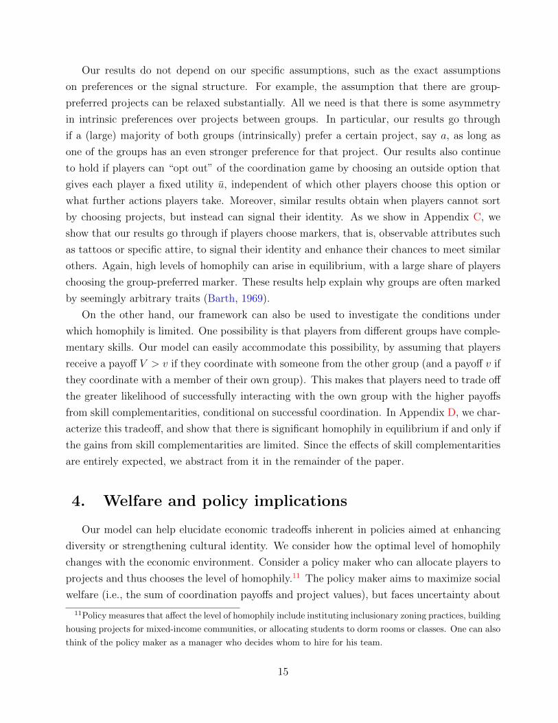
4. Welfare and policy implications

Our model can help elucidate economic tradeoffs inherent in policies aimed at enhancing

diversity or strengthening cultural identity. We consider how the optimal level of homophily

changes with the economic environment. Consider a policy maker who can allocate players to

projects and thus chooses the level of homophily.11 The policy maker aims to maximize social

welfare (i.e., the sum of coordination payoffs and project values), but faces uncertainty about

11Policy measures that affect the level of homophily include instituting inclusionary zoning practices, building

housing projects for mixed-income communities, or allocating students to dorm rooms or classes. One can also

think of the policy maker as a manager who decides whom to hire for his team.

15

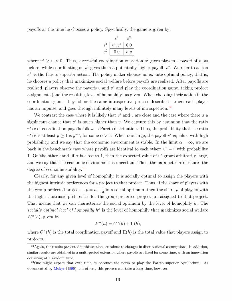
payoffs at the time he chooses a policy. Specifically, the game is given by:

s1 s2

s1 v∗,v∗ 0,0

s2 0,0 v,v

where v∗ ≥ v > 0. Thus, successful coordination on action s2 gives players a payoff of v, as

before, while coordinating on s1 gives them a potentially higher payoff, v∗. We refer to action

s1 as the Pareto superior action. The policy maker chooses an ex ante optimal policy, that is,

he chooses a policy that maximizes social welfare before payoffs are realized. After payoffs are

realized, players observe the payoffs v and v∗ and play the coordination game, taking project

assignments (and the resulting level of homophily) as given. When choosing their action in the

coordination game, they follow the same introspective process described earlier: each player

has an impulse, and goes through infinitely many levels of introspection.12

We contrast the case where it is likely that v∗ and v are close and the case where there is a

significant chance that v∗ is much higher than v. We capture this by assuming that the ratio

v∗/v of coordination payoffs follows a Pareto distribution. Thus, the probability that the ratio

v∗/v is at least y ≥ 1 is y−α, for some α > 1. When α is large, the payoff v∗ equals v with high

probability, and we say that the economic environment is stable. In the limit α =∞, we are

back in the benchmark case where payoffs are identical to each other: v∗ = v with probability

1. On the other hand, if α is close to 1, then the expected value of v∗ grows arbitrarily large,

and we say that the economic environment is uncertain. Thus, the parameter α measures the

degree of economic stability.13

Clearly, for any given level of homophily, it is socially optimal to assign the players with

the highest intrinsic preferences for a project to that project. Thus, if the share of players with

the group-preferred project is p = h+ 12

in a social optimum, then the share p of players with

the highest intrinsic preferences for the group-preferred project are assigned to that project.

That means that we can characterize the social optimum by the level of homophily h. The

socially optimal level of homophily hα is the level of homophily that maximizes social welfare

Wα(h), given by

Wα(h) = Cα(h) + Π(h),

where Cα(h) is the total coordination payoff and Π(h) is the total value that players assign to

projects.

12Again, the results presented in this section are robust to changes in distributional assumptions. In addition,

similar results are obtained in a multi-period extension where payoffs are fixed for some time, with an innovation

occurring at a random time.13One might expect that over time, it becomes the norm to play the Pareto superior equilibrium. As

documented by Mokyr (1990) and others, this process can take a long time, however.

16

4.1. Stable economic environments

In a stable economic environment, there is only a small probability that a technological

innovation increases the payoffs of one of the actions. In the limit α = ∞, the coordination

payoff to both actions is the same: the coordination payoff to either action is v. This is the

benchmark case we have studied so far. The next result shows that the socially optimal level

of homophily in a stable economic environment is arbitrarily close to the socially optimal level

of homophily in this benchmark case.

Proposition 4.1. As α goes to infinity, the socially optimal level of homophily converges

to the socially optimal level of homophily in the benchmark case where v = v∗, that is, hα

converges to h∞ as α→∞. Moreover, social welfare also converges: Wα(hα)→ W∞(h∞).

So, we can concentrate on the benchmark case where v∗ = v to study welfare in stable eco-

nomic environments. By Proposition 4.1, the results hold approximately for stable economic

environments. The next result fully characterizes the socially optimal level of homophily for

the benchmark case:

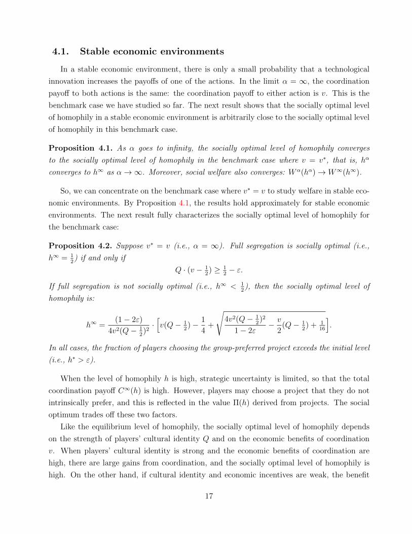
Proposition 4.2. Suppose v∗ = v (i.e., α = ∞). Full segregation is socially optimal (i.e.,

h∞ = 12) if and only if

Q · (v − 12) ≥ 1

2− ε.

If full segregation is not socially optimal (i.e., h∞ < 12), then the socially optimal level of

homophily is:

h∞ =(1− 2ε)

4v2(Q− 12)2·[v(Q− 1

2)− 1

4+

√4v2(Q− 1

2)2

1− 2ε− v

2(Q− 1

2) + 1

16

].

In all cases, the fraction of players choosing the group-preferred project exceeds the initial level

(i.e., h∗ > ε).

When the level of homophily h is high, strategic uncertainty is limited, so that the total

coordination payoff C∞(h) is high. However, players may choose a project that they do not

intrinsically prefer, and this is reflected in the value Π(h) derived from projects. The social

optimum trades off these two factors.

Like the equilibrium level of homophily, the socially optimal level of homophily depends

on the strength of players’ cultural identity Q and on the economic benefits of coordination

v. When players’ cultural identity is strong and the economic benefits of coordination are

high, there are large gains from coordination, and the socially optimal level of homophily is

high. On the other hand, if cultural identity and economic incentives are weak, the benefit

17

0.60.7

0.80.9

24

68

10

0.1

0.2

0.3

0.4

0.5

Qv

h*

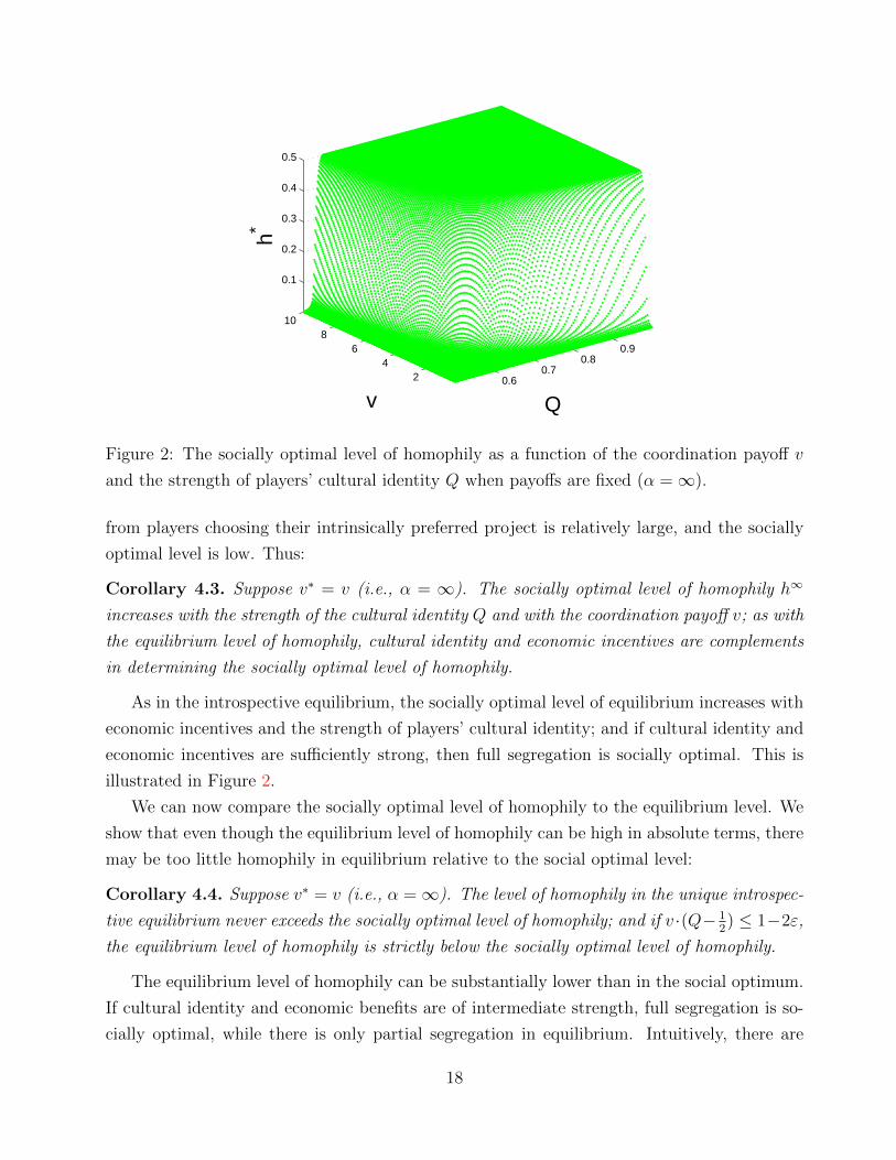
Figure 2: The socially optimal level of homophily as a function of the coordination payoff v

and the strength of players’ cultural identity Q when payoffs are fixed (α =∞).

from players choosing their intrinsically preferred project is relatively large, and the socially

optimal level is low. Thus:

Corollary 4.3. Suppose v∗ = v (i.e., α = ∞). The socially optimal level of homophily h∞

increases with the strength of the cultural identity Q and with the coordination payoff v; as with

the equilibrium level of homophily, cultural identity and economic incentives are complements

in determining the socially optimal level of homophily.

As in the introspective equilibrium, the socially optimal level of equilibrium increases with

economic incentives and the strength of players’ cultural identity; and if cultural identity and

economic incentives are sufficiently strong, then full segregation is socially optimal. This is

illustrated in Figure 2.

We can now compare the socially optimal level of homophily to the equilibrium level. We

show that even though the equilibrium level of homophily can be high in absolute terms, there

may be too little homophily in equilibrium relative to the social optimal level:

Corollary 4.4. Suppose v∗ = v (i.e., α =∞). The level of homophily in the unique introspec-

tive equilibrium never exceeds the socially optimal level of homophily; and if v ·(Q− 12) ≤ 1−2ε,

the equilibrium level of homophily is strictly below the socially optimal level of homophily.

The equilibrium level of homophily can be substantially lower than in the social optimum.

If cultural identity and economic benefits are of intermediate strength, full segregation is so-

cially optimal, while there is only partial segregation in equilibrium. Intuitively, there are

18

both positive and negative externalities associated with players choosing the group-preferred

project. Consider a player who considers switching to the group-preferred project. His switch-

ing increases the expected coordination payoff for the players with the group-preferred project,

as it increases the probability that they interact with players of their own group. On the other

hand, the switch lowers the expected coordination payoff to the players with the other project,

as there are now fewer players of their group with that project.14 Since there are more players

with the group-preferred project, the positive externality dominates the negative one, and

there tends to be too little homophily in equilibrium.

A policy maker can also influence social welfare by strengthening cultural identity, for

example by subsidizing cultural programs. Strengthening players’ cultural identity has a direct

impact on coordination payoffs by reducing strategic uncertainty. There is also an indirect

effect, through the adjustment of the level of homophily in response to changes in cultural

identity. This further reduces strategic uncertainty. The next result shows that the overall

effect on social welfare is positive.

Corollary 4.5. Suppose v∗ = v (i.e., α =∞). Policies that strengthen cultural identity lead

to more homophily and improve welfare.

The results are illustrated in Figure 3. These results may explain the popularity of policies

that aim to strengthen cultural identity. For example, a strong organizational culture is often

described as a key to a company’s success (e.g., Tichy and Sherman, 2005). In 19th-century

Europe, newly formed nation states built national museums to strengthen national identity

(Macdonald, 2012). And social movements in 19th-century U.S. stimulated public school

enrollment to build a new, common identity (Meyer et al., 1979). While such narratives are

both widespread and intuitive, they are difficult to formalize within the standard framework.

First, the standard framework does not explicitly model cultural identity. If we augment the

standard framework with a signal structure so as to capture context-dependent norms and

cultural identity, then the welfare implications of strengthening players’ cultural identity may

be ambiguous. This is because there are multiple (correlated) equilibria. As cultural identity

is strengthened, the set of equilibria changes, and there are instances where strengthening

players’ cultural identity gives rise to new equilibria with lower welfare.15

14A player’s choice also affects the payoffs of members of the other group. These effects go in the same

direction.15Since any introspective equilibrium is a correlated equilibrium, there is a correlated equilibrium where

strengthening cultural identity improves welfare. However, it is not clear how this equilibrium can be selected

using standard methods.

19

0.55 0.6 0.65 0.7 0.75 0.8 0.85 0.9 0.95

0.55

0.6

0.65

0.7

0.75

0.8

0.85

0.9

0.95

1

Q

h

(a)

0.55 0.6 0.65 0.7 0.75 0.8 0.85 0.9 0.951

1.1

1.2

1.3

1.4

1.5

1.6

1.7

1.8

Q

W

(b)

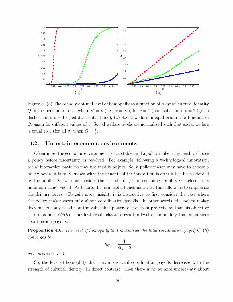
Figure 3: (a) The socially optimal level of homophily as a function of players’ cultural identity

Q in the benchmark case where v∗ = v (i.e., α =∞), for v = 1 (blue solid line), v = 2 (green

dashed line), v = 10 (red dash-dotted line); (b) Social welfare in equilibrium as a function of

Q, again for different values of v. Social welfare levels are normalized such that social welfare

is equal to 1 (for all v) when Q = 12.

4.2. Uncertain economic environments

Oftentimes, the economic environment is not stable, and a policy maker may need to choose

a policy before uncertainty is resolved. For example, following a technological innovation,

social interaction patterns may not readily adjust. So, a policy maker may have to choose a

policy before it is fully known what the benefits of the innovation is after it has been adopted

by the public. So, we now consider the case the degree of economic stability α is close to its

minimum value, viz., 1. As before, this is a useful benchmark case that allows us to emphasize

the driving forces. To gain more insight, it is instructive to first consider the case where

the policy maker cares only about coordination payoffs. In other words, the policy maker

does not put any weight on the value that players derive from projects, so that his objective

is to maximize Cα(h). Our first result characterizes the level of homophily that maximizes

coordination payoffs.

Proposition 4.6. The level of homophily that maximizes the total coordination payoff Cα(h)

converges to

hC :=1

8Q− 2

as α decreases to 1.

So, the level of homophily that maximizes total coordination payoffs decreases with the

strength of cultural identity. In direct contrast, when there is no ex ante uncertainty about

20

payoffs (i.e., v∗ = v with probability 1), a policy maker that aims to maximize coordination

payoffs (as opposed to social welfare) would opt for full segregation, for any value of the

parameters.

While the result may appear surprising at first sight, there is a clear intuition. To achieve

the high payoff v∗, players may have to go against their instincts when their initial impulse is

to choose the other action. If players go against their impulse, they face the risk of miscoor-

dinating. This risk is smaller for the minority because they are less likely to meet a similar

opponent and so their initial impulse is a weaker signal. So, if v∗ can be moderately high

then the minority may decide to play the Pareto superior action even if their impulse says

otherwise. But this does not necessarily induce the majority to go against their impulse to

choose the Pareto superior action. The majority has an incentive to choose the Pareto su-

perior action only if the minority is sizeable. So, a policy maker interested in maximizing

coordination payoffs must strike a balance: the minority needs to be small enough so that it

faces limited pressure to conform, while it has the critical mass to influence the majority. This

result is consistent with work on team composition and creativity. For example, De Dreu and

West (2001) and Gibson and Vermeulen (2003) show empirically that minority dissent can

make teams more innovative (i.e., choose the high-payoff option), but only if the minority can

influence the decision-making process of the majority.

In the case that project payoffs are also taken into account, the same intuitions apply,

but the optimal level of homophily is no longer monotonic in the strength of players’ cultural

identity:

Proposition 4.7. If the economic environment is uncertain (i.e., α close to 1), there is

Q∗ ∈ (12, 1) such that:

• If the strength of players’ cultural identity Q is below Q∗, then the socially optimal level

of homophily is strictly below the level hC that maximizes coordination payoffs;

• If the strength of players’ cultural identity Q exceeds Q∗, then the socially optimal level

of homophily and the level hC that maximizes coordination payoffs coincide.

The threshold Q∗ decreases with the coordination payoff v.

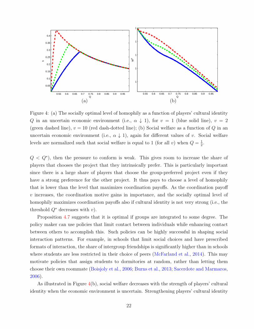
So, there are two regimes, as shown in Figure 4(a). If cultural identity is strong (i.e.,

Q > Q∗), there is a strong pressure to conform. Any level of homophily that deviates from the

level hC that maximizes coordination payoffs results in a low probability that players choose

the Pareto superior action.Hence, it is socially optimal to choose the level of homophily to

maximize coordination payoffs. On the other hand, if players’ cultural identity is weak (i.e.,

21

0.55 0.6 0.65 0.7 0.75 0.8 0.85 0.9 0.95

0.05

0.1

0.15

0.2

0.25

0.3

0.35

0.4

Q

h

(a)

0.55 0.6 0.65 0.7 0.75 0.8 0.85 0.9 0.95

1

1

1

1

1

Q

Wα

(b)

Figure 4: (a) The socially optimal level of homophily as a function of players’ cultural identity

Q in an uncertain economic environment (i.e., α ↓ 1), for v = 1 (blue solid line), v = 2

(green dashed line), v = 10 (red dash-dotted line); (b) Social welfare as a function of Q in an

uncertain economic environment (i.e., α ↓ 1), again for different values of v. Social welfare

levels are normalized such that social welfare is equal to 1 (for all v) when Q = 12.

Q < Q∗), then the pressure to conform is weak. This gives room to increase the share of

players that chooses the project that they intrinsically prefer. This is particularly important

since there is a large share of players that choose the group-preferred project even if they

have a strong preference for the other project. It thus pays to choose a level of homophily

that is lower than the level that maximizes coordination payoffs. As the coordination payoff

v increases, the coordination motive gains in importance, and the socially optimal level of

homophily maximizes coordination payoffs also if cultural identity is not very strong (i.e., the

threshold Q∗ decreases with v).

Proposition 4.7 suggests that it is optimal if groups are integrated to some degree. The

policy maker can use policies that limit contact between individuals while enhancing contact

between others to accomplish this. Such policies can be highly successful in shaping social

interaction patterns. For example, in schools that limit social choices and have prescribed

formats of interaction, the share of intergroup friendships is significantly higher than in schools

where students are less restricted in their choice of peers (McFarland et al., 2014). This may

motivate policies that assign students to dormitories at random, rather than letting them

choose their own roommate (Boisjoly et al., 2006; Burns et al., 2013; Sacerdote and Marmaros,

2006).

As illustrated in Figure 4(b), social welfare decreases with the strength of players’ cultural

identity when the economic environment is uncertain. Strengthening players’ cultural identity

22

enhances the pressure to conform. That makes it harder for a policy maker to strike a good

balance and choose a level of homophily such that the minority is small enough for it to face

limited pressure to conform, yet large enough so that it can influence the majority. There is

thus a marked contrast with the results for stable economic environments. While in a stable

economic environment, strengthening cultural identity enhances players’ ability to coordinate,

in an uncertain economic environment a strong cultural identity can be harmful, as it increases

the pressure to conform. While the welfare implications of policies that strengthen cultural

identity are different for stable and economic environments, the results really present two

sides of the same coin: strengthening cultural identity mitigates strategic uncertainty, which

increases the pressure to conform. In a stable economic environment, this is beneficial, but in

an uncertain economic environment, the pressure to conform reduces social welfare.

Once again, our results are consistent with common narratives on the trade-offs involved in

setting social policy. In particular, our analysis can explain why segregated societies may find

it harder to break out of low-payoff equilibria than more open-minded societies, consistent with

historical data (Mokyr, 1990). It also allows us to explore the interaction between cultural

identity and social structure. Our analysis shows that a more integrated society or societies

with a weak cultural identity gives rise to more behavioral variation, and this gives the society

an opportunity to escape Pareto inferior equilibria.

While these insights are intuitive, standard equilibrium analysis does produces these re-

sults. In a standard equilibrium framework, the Pareto superior equilibrium is arguably focal,

and dynamic processes that operate through the gradual accretion of precedent indeed predict

this outcome (Young, 1993). However, neither the standard equilibrium framework nor such

a dynamic framework can explain why certain societies or cultures find it easier to coordinate

on the Pareto superior outcome than others, as documented by Mokyr (1990) and others.

Our analysis shows that a more integrated society or societies with a weak cultural identity

gives rise to more behavioral variation, and this gives the society an opportunity to escape

Pareto inferior equilibria. These driving forces, though intuitive, cannot be captured by either

a standard equilibrium analysis or in a dynamic model.

5. Network formation

In many situations, people can choose how many people they interact with. So, we extend

the basic model to allow players to choose how much effort they want to invest in meeting

others. We show that the basic mechanisms that drive the tendencies to segregate may be

reinforced, and that the model gives rise to network properties that are commonly observed

in social and economic networks.

23

To analyze this setting, it is convenient to work with a finite (but large) set of players.16

Each group G = A,B has N players, so that the total number of players is 2N . Players

simultaneously choose effort levels and projects in the first stage. They then interact in the

coordination game (with fixed payoffs, i.e., v∗ = v). Effort is costly: a player that invests

effort e pays a cost ce2/2. By investing effort, however, a player meets more partners to play

the coordination game with (in expectation). Specifically, if two players j, ` have chosen the

same project π = a, b, and invest effort ej and e`, respectively, then the probability that they

are matched (and play the coordination game) is

ej · e`Eπ

,

where Eπ is the total effort of the players with project π.17 Thus, efforts are complements:

players tend to meet each other when they both invest time and resources. This is related

to the assumption of bilateral consent in deterministic models of network formation (Jackson

and Wolinsky, 1996). By normalizing by the total effort Eπ, we ensure that the network does

not become arbitrarily dense as the number of players grows large.18 So, the probability of

being matched with a member of the own group is endogenous here, as in Section 3. Matching

probabilities are now affected not only by players’ project choice, as in Section 3, but also by

their effort levels.

As before, at level 0 players choose the project that they intrinsically prefer. So, the

probability that a player chooses the group-preferred project is 12

+ ε. In addition, each player

chooses some default effort e0 > 0, independent of his project or group. At higher levels k,

each player formulates a best response to their partners choices at level k− 1. As before, each

player receives a (single) signal that tells him which action is appropriate in the coordination

game. He then plays the coordination game with each of the players he is matched to.19

A preliminary result is that the limiting behavior is well-defined, and that it is independent

of the choice of effort at level 0.

Lemma 5.1. The limiting probability p and the limiting effort choices exist and do not depend

on the effort choice at level 0.

16Defining networks with a continuum of players gives rise to technical problems. Our results in Sections

2 and 3 continue to hold under the present formulation of the model (with a finite player set), though the

notation becomes more tedious.17To be precise, to get a well-defined probability, if Eπ = 0, we take the probability to be 0; and if ej ·e` > Eπ,

we take the probability to be 1.18See, e.g., Cabrales et al. (2011) and Galeotti and Merlino (2014) for applications of this model in economics.19We allow players to take different actions in each of the (two-player) coordination games he is involved in.

Nevertheless, in any introspective equilibrium, a player chooses the same action in all his interactions, as it is

optimal for him to follow his impulse (Proposition 2.1).

24

0

1

2

3

4

5

0.50.55

0.60.65

0.70.75

0.80.85

0.90.95

1

0

0.05

0.1

0.15

0.2

0.25

0.3

0.35

0.4

0.45

0.5

vQ

h

Figure 5: The level of homophily h as a function of the coordination payoff v and the strength

of players’ cultural identity Q (c = 1).

As before, we have a unique introspective equilibrium, with potentially high levels of

homophily:

Proposition 5.2. There is a unique introspective equilibrium. In the unique equilibrium,

all players choose positive effort. Players that have chosen the group-preferred project exert

strictly more effort than players with the other project. In all cases, the fraction of players

choosing the group-preferred project exceeds the initial level (i.e., h > ε).

As before, players segregate for strategic reasons and the level of homophily is greater than

what would be expected on the basis of intrinsic preferences alone (i.e., h > ε). Importantly,

players with the group-preferred project invest more effort in equilibrium than players with the

other project. This is intuitive: a player with the group-preferred project has a high chance

of meeting people from her own group, and thus a high chance of coordinating successfully.

In turn, this reinforces the incentives to segregate.

Figure 5 illustrates the comparative statics of the unique equilibrium. As before, the

level of homophily increases with the strength of players’ cultural identity and with economic

incentives, and the two are complements. While the proof of Proposition 5.2 provides a full

characterization of the equilibrium, the comparative statics cannot be analyzed analytically, as

the effort levels and the level of homophily depend on each other in intricate ways. We therefore

focus on deriving analytical results for the case where the network becomes arbitrarily large

25

(i.e., |N | → ∞). As a first step, we give an explicit characterization of the unique introspective

equilibrium:

Proposition 5.3. Consider the limit where the number of players in each group goes to infin-

ity. The effort chosen by the players with the group-preferred project in the unique introspective

equilibrium converges to

e∗ =v

4c·

(1 + 2Q− 1

2h+

√4Q2 − 1 +

1

4h2

),

while the effort chosen by the players with the other project converges to

e− =v

c· (Q+ 1

2)− e∗,

which is strictly smaller than the effort e∗ (while positive).

Proposition 5.3 shows that in the unique introspective equilibrium, the effort levels depend

on the level of homophily. The level of homophily, in turn, is a function of the equilibrium

effort levels. For example, by increasing her effort, an A-player with the group-preferred

project a increases the probability that players from both groups interact with her and thus

with members from group A. This makes project a more attractive for members from group

A, strengthening the incentives for players from group A to choose project a, and this leads

to higher levels of homophily. Conversely, if more players choose the group-preferred project,

this strengthens the incentives of players with the group-preferred project to invest effort, as

it increases their chances of meeting a player from their own group. This, in turn, further

increases the chances for players with the group-preferred project of meeting someone from

the own group, reinforcing the incentives to segregate. On the other hand, if effort is low,

then the incentives to segregate are attenuated, as the probability of meeting similar others is

small. This, in turn, reduces the incentives to invest effort.

As a result of this feedback loop, there are two different regimes. If effort costs are small

relative to the benefits of coordinating, then players are willing to exert high effort, which in

turn leads more players to choose the group-preferred project, further enhancing the incentives

to invest effort. In that case, groups are segregated, and players are densely connected.

Importantly, players with the group-preferred project face much stronger incentives to invest

effort than players with the other project, as players with the group-preferred project have

a high chance of interacting with players from their own group. On the other hand, if effort

costs are sufficiently high, then the net benefit of interacting with others is small, even if

an organization is fully segregated. In that case, choices are guided primarily by intrinsic

preferences over projects, and the level of homophily is low. As a result, players face roughly

26

the same incentives to invest effort, regardless of their project choice, and all players have

approximately the same number of connections. Hence, high levels of homophily go hand in

hand with inequality in the number of connections that players have. The following result

makes this precise:20

Proposition 5.4. Consider the limit where the number of players in each group goes to in-

finity. In the unique introspective equilibrium, the distribution of connections of players with

the group-preferred project first-order stochastically dominates the distribution of the number

of connections of players with the other project. The difference in the expected number of con-

nections of the players with the group-preferred project and the other project strictly increases

with the level of homophily.

These results are consistent with empirical evidence. More homogeneous groups have a

higher level of social interactions (Alesina and La Ferrara, 2000); and the distribution of the

number of connections in social and economic networks has considerable variance (Jackson,

2008). Furthermore, consistent with the theoretical results, friendships are often biased to-

wards own-group friendships, and larger groups form more friendships per capita (Currarini

et al., 2009).

Our results put restrictions on the type of networks that can be observed. When relative

benefits v/c are high and there is a strong cultural identity Q, networks are dense and are

characterized by high levels of homophily and a skewed distribution of the number of connec-

tions that players have. Moreover, the network consists of a tightly connected core of players

from one group, with a smaller periphery of players from the other group. When v/c increases

further, segregation is complete (h = 12), and a densely connected homogenous network results.

On the other hand, when economic benefits are limited and cultural identity is weak, networks

are disconnected, and feature low levels of homophily and limited variation in the number of

connections. Most data on network on social and economic networks is consistent with the

case where there is a strong cultural identity and sizeable economic benefits to coordination,

with many networks featuring high levels of homophily, a core-periphery structure, high levels

of connectedness, and a skewed degree distribution (Jackson, 2008). More research, however,

is needed, to establish the extent that these observations can be attributed to the economic

and cultural factors related to strategic uncertainty.

20This result follows directly from Proposition 5.2 and Theorem 3.13 of Bollobas et al. (2007). In fact, more

can be said: the number of connections of a player with the group-preferred project converges to a Poisson

random variable with parameter e∗, and the number of connections of players with the other project converges

to a Poisson random variable with parameter e− < e∗.

27

6. Conclusions

This paper introduces a novel approach to model players’ introspective process, grounded

in the Theory of Mind. We show that high levels of homophily are possible even if there are no

group-specific externalities and no direct preference for interacting with similar players. Mod-

eling players’ introspective process explicitly makes it possible to derive unique predictions and

robust and intuitive comparative statics results. Consistent with empirical and experimental

evidence, homophily is high when cultural identities are strong, benefits from coordination are

large, and networks are formed endogenously. The theory elucidates how the socially optimal

level of homophily varies with the economic environment. While segregation can be optimal in

a stable economic environment, diversity and integration is better in uncertain environments.

There are a number of directions for future research. On the methodological side, we plan

to examine the potential of our approach in general games. In ongoing experimental work, we

are investigating the extent to which beliefs and the need to reduce strategic uncertainty drives

homophily. Another promising direction is to study how players’ cultural identity coevolves

with social structure. Indeed, members of inclusive organizations may gain a better under-

standing of the cultural background of others, while individuals belonging to more segregated

organizations specialize in their own culture. If that is the case, different social structures

may develop depending on initial conditions, and interaction patterns may be persistent, con-

sistent with empirical evidence (Ellison and Powers, 1994). Opening the black box of how

intergroup contact affects intergroup understanding may also make it possible to assess which

types of interventions are welfare improving: for example, is it important that individuals be-

come sensitive to each other’s culture, or is it necessary that they develop a joint identity? To

answer these types of questions, it is critical to model cultural identity and players’ reasoning

processes, and this paper presents a first step in this direction.

A. Intrinsic preferences

We denote the values of an A-player j for projects a and b are denoted by wA,aj and

wA,bj , respectively; likewise, the values of a B-player for projects b and a are wB,bj and wB,aj ,

respectively. As noted in the main text, the values wA,aj and wA,bj are drawn from the uniform

distribution on [0, 1] and [0, 1 − 2ε], respectively. Likewise, wB,bj and wB,aj are uniformly

distributed on [0, 1] and [0, 1−2ε]. All values are drawn independently (across players, projects,

and groups). So, players in group A (on average) intrinsically prefer project a (in the sense of

first-order stochastic dominance) over project b; see Figure 6. Likewise, on average, players in

group B have an intrinsic preference for b.

28

−0.2 0 0.2 0.4 0.6 0.8 1 1.20

0.1

0.2

0.3

0.4

0.5

0.6

0.7

0.8

0.9

1

y

Pro

b(w

jA,a

≤ y)

, Pro

b(w

jA,b

≤ y)

Figure 6: The cumulative distribution functions of wA,ai (solid line) and wA,bi (dashed line) for

x = 0.75.

Given that the values are uniformly and independently distributed, the distribution of the

difference wA,aj −wB,aj in values for an A-player is given by the so-called trapezoidal distribution.

That is, if we define x := 1−2ε, we can define the tail distribution Hε(y) := P(wA,aj −wA,bj ≥ y)

by

Hε(y) =

1 if y < −(1− 2ε);

1− 12−4ε · (1− 2ε+ y)2 if y ∈ [−(1− 2ε), 0);

1− 12· (1− 2ε)− y if y ∈ [0, 2ε);

1

4(12−ε)· (1− y)2 if y ∈ [2ε, 1];

0 otherwise.

By symmetry, the probability P(wB,bj −wB,aj ≥ y) that the difference in values for the B-player

is at least y is also given by Hε(y). So, we can identify wA,aj − wA,bj and wB,bj − wB,aj with the

same random variable, denoted ∆j, with tail distribution Hε(·); see Figure 7.

The probability that A-players prefer the a-project, or, equivalently, the share of A-players

that intrinsically prefer a (i.e., wA,aj − wA,bj > 0), is 1 − 12x = 1

2+ ε, and similarly for the

B-players and project b.

29

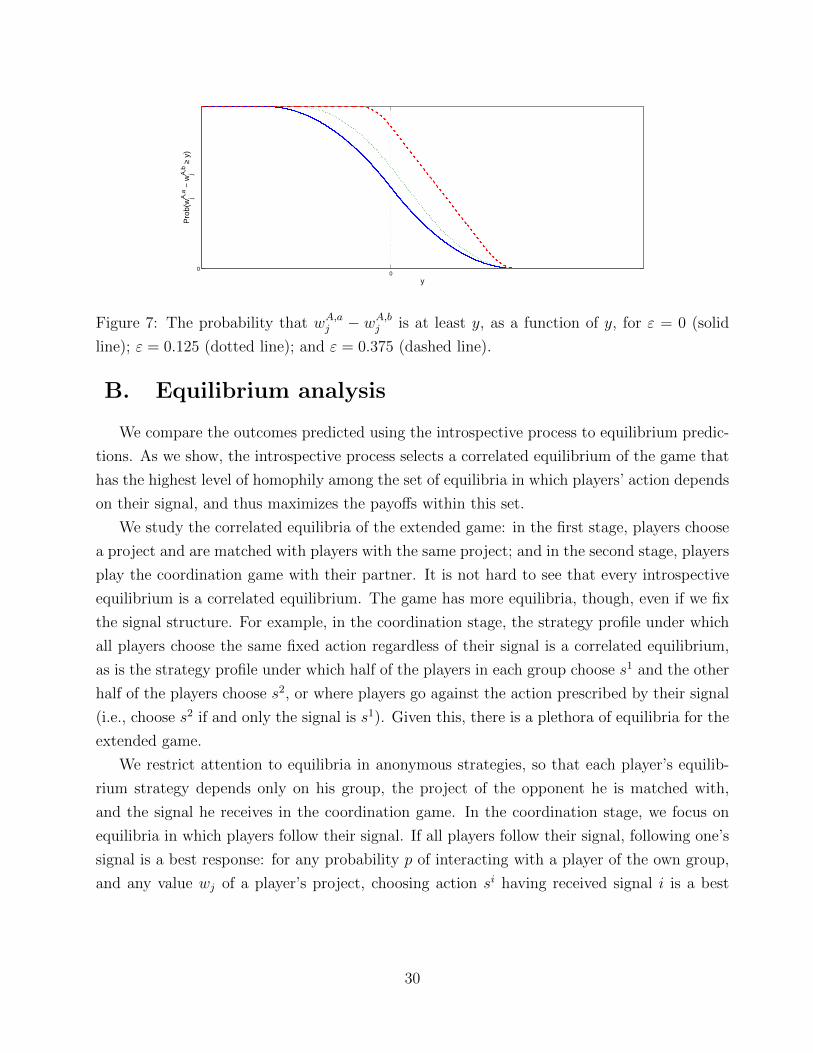
00

y

Pro

b(w

A,a

j −

wA

,bj

≥ y

)

Figure 7: The probability that wA,aj − wA,bj is at least y, as a function of y, for ε = 0 (solid

line); ε = 0.125 (dotted line); and ε = 0.375 (dashed line).

B. Equilibrium analysis

We compare the outcomes predicted using the introspective process to equilibrium predic-

tions. As we show, the introspective process selects a correlated equilibrium of the game that

has the highest level of homophily among the set of equilibria in which players’ action depends

on their signal, and thus maximizes the payoffs within this set.

We study the correlated equilibria of the extended game: in the first stage, players choose

a project and are matched with players with the same project; and in the second stage, players

play the coordination game with their partner. It is not hard to see that every introspective

equilibrium is a correlated equilibrium. The game has more equilibria, though, even if we fix

the signal structure. For example, in the coordination stage, the strategy profile under which

all players choose the same fixed action regardless of their signal is a correlated equilibrium,

as is the strategy profile under which half of the players in each group choose s1 and the other

half of the players choose s2, or where players go against the action prescribed by their signal

(i.e., choose s2 if and only the signal is s1). Given this, there is a plethora of equilibria for the

extended game.

We restrict attention to equilibria in anonymous strategies, so that each player’s equilib-

rium strategy depends only on his group, the project of the opponent he is matched with,

and the signal he receives in the coordination game. In the coordination stage, we focus on

equilibria in which players follow their signal. If all players follow their signal, following one’s

signal is a best response: for any probability p of interacting with a player of the own group,

and any value wj of a player’s project, choosing action si having received signal i is a best

30

response if and only if[pQ+ (1− p) · 1

2

]· v + wj ≥

[p · (1−Q) + (1− p) · 1

2

]· v + wj.

This inequality is always satisfied, as Q > 12.

So, it remains to consider the matching stage. Suppose that mA,a and mB,b are the shares

of A-players and B-players that choose projects a and b, respectively. Then, the probability

that a player with project a belongs to group A is

pA,a =mA,a

mA,a + 1−mB,b;

similarly, the probability that a player with project b belongs to group B equals

pB,b =mB,b

mB,b + 1−mA,a.

An A-player with intrinsic values wA,aj and wA,bj for the projects chooses project a if and only

if [pA,aQ+ (1− pA,a) · 1

2

]· v + wA,aj ≥

[(1− pB,b) ·Q+ pB,b 1

2

]· v + wA,bj ;

or, equivalently,

wA,aj − wA,bj ≥ −(pA,a + pB,b − 1) · β,

where we have defined β := v · (Q − 12). Similarly, a B-player with intrinsic values wB,bj and

wB,aj chooses b if and only if

wB,bj − wB,aj ≥ −(pA,a + pB,b − 1) · β

In equilibrium, we must have that

P(wA,aj − wA,bj ≥ −(pA,a + pB,b − 1) · β

)=mA,a; and

P(wB,bj − w

B,aj ≥ −(pA,a + pB,b − 1) · β

)=mB,b.

Because the random variables wA,aj − wA,bj and wB,bj − wB,aj have the same distribution (cf.

Appendix A), it follows that mA,a = mB,b and pA,a = pB,b in equilibrium. Defining p := pA,a

(and recalling the notation ∆j := wA,aj − wA,bj from Appendix A), the equilibrium condition

reduces to

P(∆j ≥ −(2p− 1) · β) = p. (B.1)

Thus, equilibrium strategies are characterized by a fixed point p of Equation (B.1).

It is easy to see that the introspective equilibrium characterized in Proposition 3.2 is an

equilibrium. However, the game has more equilibria. The point p = 0 is a fixed point of (B.1)

31

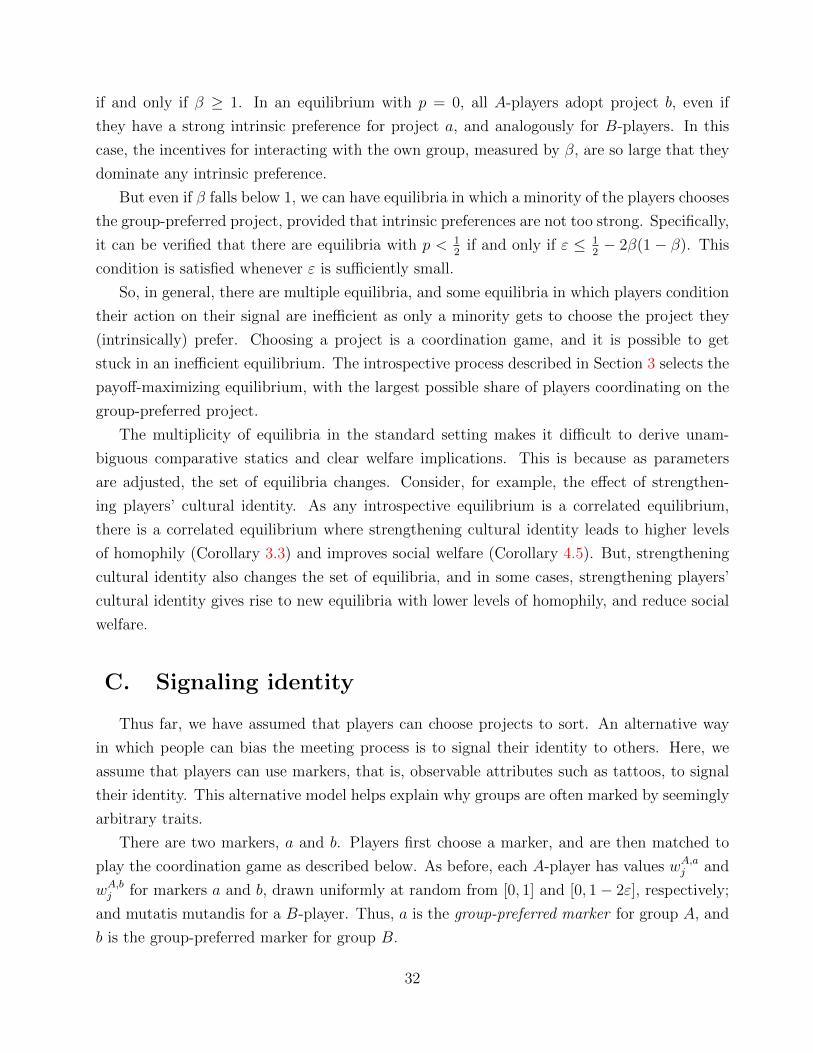
if and only if β ≥ 1. In an equilibrium with p = 0, all A-players adopt project b, even if

they have a strong intrinsic preference for project a, and analogously for B-players. In this

case, the incentives for interacting with the own group, measured by β, are so large that they

dominate any intrinsic preference.

But even if β falls below 1, we can have equilibria in which a minority of the players chooses

the group-preferred project, provided that intrinsic preferences are not too strong. Specifically,

it can be verified that there are equilibria with p < 12

if and only if ε ≤ 12− 2β(1 − β). This

condition is satisfied whenever ε is sufficiently small.

So, in general, there are multiple equilibria, and some equilibria in which players condition

their action on their signal are inefficient as only a minority gets to choose the project they

(intrinsically) prefer. Choosing a project is a coordination game, and it is possible to get

stuck in an inefficient equilibrium. The introspective process described in Section 3 selects the

payoff-maximizing equilibrium, with the largest possible share of players coordinating on the

group-preferred project.

The multiplicity of equilibria in the standard setting makes it difficult to derive unam-

biguous comparative statics and clear welfare implications. This is because as parameters

are adjusted, the set of equilibria changes. Consider, for example, the effect of strengthen-

ing players’ cultural identity. As any introspective equilibrium is a correlated equilibrium,

there is a correlated equilibrium where strengthening cultural identity leads to higher levels

of homophily (Corollary 3.3) and improves social welfare (Corollary 4.5). But, strengthening

cultural identity also changes the set of equilibria, and in some cases, strengthening players’

cultural identity gives rise to new equilibria with lower levels of homophily, and reduce social

welfare.

C. Signaling identity

Thus far, we have assumed that players can choose projects to sort. An alternative way

in which people can bias the meeting process is to signal their identity to others. Here, we

assume that players can use markers, that is, observable attributes such as tattoos, to signal

their identity. This alternative model helps explain why groups are often marked by seemingly

arbitrary traits.

There are two markers, a and b. Players first choose a marker, and are then matched to

play the coordination game as described below. As before, each A-player has values wA,aj and

wA,bj for markers a and b, drawn uniformly at random from [0, 1] and [0, 1− 2ε], respectively;

and mutatis mutandis for a B-player. Thus, a is the group-preferred marker for group A, and

b is the group-preferred marker for group B.

32

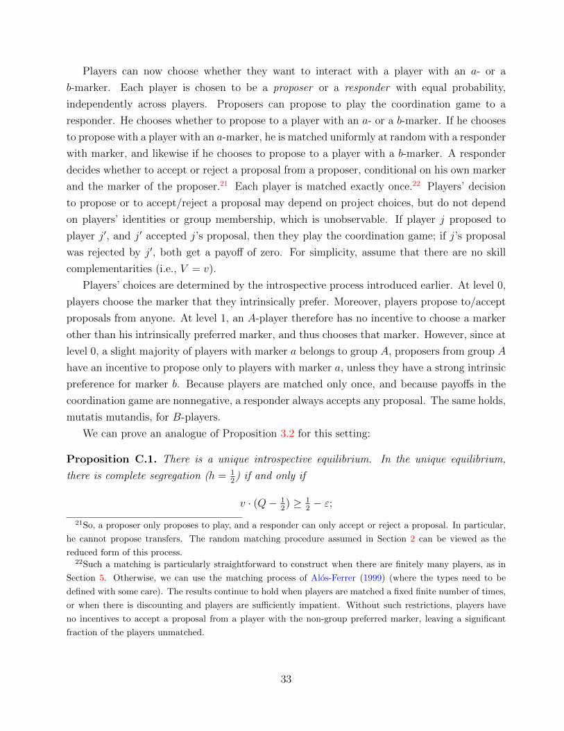
Players can now choose whether they want to interact with a player with an a- or a

b-marker. Each player is chosen to be a proposer or a responder with equal probability,

independently across players. Proposers can propose to play the coordination game to a

responder. He chooses whether to propose to a player with an a- or a b-marker. If he chooses

to propose with a player with an a-marker, he is matched uniformly at random with a responder

with marker, and likewise if he chooses to propose to a player with a b-marker. A responder

decides whether to accept or reject a proposal from a proposer, conditional on his own marker

and the marker of the proposer.21 Each player is matched exactly once.22 Players’ decision

to propose or to accept/reject a proposal may depend on project choices, but do not depend

on players’ identities or group membership, which is unobservable. If player j proposed to

player j′, and j′ accepted j’s proposal, then they play the coordination game; if j’s proposal

was rejected by j′, both get a payoff of zero. For simplicity, assume that there are no skill

complementarities (i.e., V = v).

Players’ choices are determined by the introspective process introduced earlier. At level 0,

players choose the marker that they intrinsically prefer. Moreover, players propose to/accept

proposals from anyone. At level 1, an A-player therefore has no incentive to choose a marker

other than his intrinsically preferred marker, and thus chooses that marker. However, since at

level 0, a slight majority of players with marker a belongs to group A, proposers from group A

have an incentive to propose only to players with marker a, unless they have a strong intrinsic

preference for marker b. Because players are matched only once, and because payoffs in the

coordination game are nonnegative, a responder always accepts any proposal. The same holds,

mutatis mutandis, for B-players.

We can prove an analogue of Proposition 3.2 for this setting:

Proposition C.1. There is a unique introspective equilibrium. In the unique equilibrium,

there is complete segregation (h = 12) if and only if

v · (Q− 12) ≥ 1

2− ε;

21So, a proposer only proposes to play, and a responder can only accept or reject a proposal. In particular,

he cannot propose transfers. The random matching procedure assumed in Section 2 can be viewed as the

reduced form of this process.22Such a matching is particularly straightforward to construct when there are finitely many players, as in

Section 5. Otherwise, we can use the matching process of Alos-Ferrer (1999) (where the types need to be

defined with some care). The results continue to hold when players are matched a fixed finite number of times,

or when there is discounting and players are sufficiently impatient. Without such restrictions, players have

no incentives to accept a proposal from a player with the non-group preferred marker, leaving a significant

fraction of the players unmatched.

33

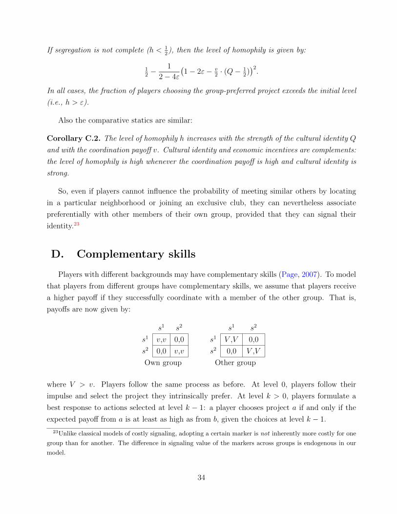
If segregation is not complete (h < 12), then the level of homophily is given by:

12− 1

2− 4ε

(1− 2ε− v

2· (Q− 1

2))2.

In all cases, the fraction of players choosing the group-preferred project exceeds the initial level

(i.e., h > ε).

Also the comparative statics are similar:

Corollary C.2. The level of homophily h increases with the strength of the cultural identity Q

and with the coordination payoff v. Cultural identity and economic incentives are complements:

the level of homophily is high whenever the coordination payoff is high and cultural identity is

strong.

So, even if players cannot influence the probability of meeting similar others by locating

in a particular neighborhood or joining an exclusive club, they can nevertheless associate

preferentially with other members of their own group, provided that they can signal their

identity.23

D. Complementary skills

Players with different backgrounds may have complementary skills (Page, 2007). To model

that players from different groups have complementary skills, we assume that players receive

a higher payoff if they successfully coordinate with a member of the other group. That is,

payoffs are now given by:

s1 s2

s1 v,v 0,0

s2 0,0 v,v

Own group

s1 s2

s1 V ,V 0,0

s2 0,0 V ,V

Other group

where V > v. Players follow the same process as before. At level 0, players follow their

impulse and select the project they intrinsically prefer. At level k > 0, players formulate a

best response to actions selected at level k − 1: a player chooses project a if and only if the

expected payoff from a is at least as high as from b, given the choices at level k − 1.

23Unlike classical models of costly signaling, adopting a certain marker is not inherently more costly for one

group than for another. The difference in signaling value of the markers across groups is endogenous in our

model.

34

If the probability that players are matched with an opponent of the same group is p ∈ (0, 1],

then a player’s expected payoff is

pQv + (1− p)12V,

so the marginal benefit of interacting with the own group is

βCS := Qv − 12V.

Note that βCS can be positive or negative, depending on the relative strengths of players’

cultural identity, economic incentives, and skill complementarities. If βCS < 0, the effect of

skill complementarities on payoffs is greater than the benefit of interacting with the own group,

and we say that skill complementarities dominate. Otherwise, if βCS > 0, players benefit

from interacting with members of their own group as that reduces strategic uncertainty. The

analysis from Section 3 extends directly to this case. We therefore focus on the case βCS < 0

here.

As before, let pak be the fraction of A-players among those with project a at level k, and

let pbk be the fraction of B-players among those with project b at level k. We can prove the

analogue of Lemma 3.1 for this setting:24

Lemma D.1. Suppose skill complementarities dominate and that βCS > −12. The limit pπ of

the fractions pπ0 , pπ1 , . . . exists for each project π = a, b. Moreover, the limits are the same for

both projects: pa = pb.

Proof. Suppose βCS ∈ (−12, 0). By an argument similar to the one in the proof of Lemma

3.1, it follows that the sequence {pπk}k is weakly decreasing and bounded for every project π.

Moreover, pπk <12

+ ε for all k. Again, by the monotone convergence theorem, the sequences

{pak}k and {pbk}k converge to a common limit p. �

The next result shows that there is a unique introspective equilibrium also in this case, and

characterizes the equilibrium level of homophily.

Proposition D.2. Suppose skill complementarities dominate and that βCS > −12. There is

a unique introspective equilibrium. The equilibrium fraction of players choosing the group-

preferred project is strictly below the initial level (i.e., h < ε), and is given by

h =ε

1− 2(Qv − 12V )

> 0.

24It can be checked that if βCS < − 12 , then the sequence pπ0 , p

π1 , . . . does not settle down. Intuitively, players

have an incentive to “flee” from players of their own group to reap the high payoffs from interacting with the

other group. For example, if A-players make up the majority of players with project a at level k, then even

an A-player for whom it is optimal to choose project a at level k may find it beneficial to choose project b at

level k + 1, and A-players form the minority of players with project a at that level.

35

Proof. By Lemma D.1, pk ≤ pk−1 for all k. By the monotone sequence convergence theorem,

p = infk pk. As before, we can find p by solving the fixed-point equation

p = Hε(−(2p− 1) · βCS).

Writing y := −(2p− 1) · βCS, we now need to consider two regimes: y ∈ (0, ε) and y ∈ [2ε, 1]

(cf. Appendix A). In the second regime, Hε(y) = 12x

(1 − y)2, and the fixed-point equation

p(y) = Hε(y) has two roots y1, y2 that lie outside the domain (0, 2ε). So consider the first

regime, where Hε(y) = 1 − 12x − y. The fixed-point equation has a unique solution y∗, with

corresponding limiting probability

p = 12− ε

2βCS − 1.

It can be checked that p is increasing in βCS, and lies in (12, 12

+ ε) for βCS < 0. �

This is consistent with empirical evidence that skill complementarities across groups can

reduce the level of homophily (Aldrich and Kim, 2007). Our model shows how these factors in-

teract: if cultural identities are weak, then complementarities of skills become more important

in shaping interactions.

The next result characterizes the socially optimal level of homophily in the presence of

skill complementarities.

Proposition D.3. Suppose skill complementarities dominate. Full segregation is never opti-

mal. The socially optimal level of homophily is given by:

h∗ = 4(Qv − 12V )(1− 2ε) + 5ε− 2 +

√4(Qv − 1

2V )2 − 5(Qv − 1

2V ) + 1 +

(Qv − 12V )

1− 2ε.

The fraction of players choosing the group-preferred project in the social optimum is below the

initial level (i.e., h∗ < ε).

This result follows readily from the proof of Proposition 4.2 if we modify the expression

C∞(p) for the coordination payoffs to take into account that coordinating with a member of

the other group provides payoff V ≥ v.

Proposition D.3 demonstrates that if skill complementarities dominate, there can be too

much homophily in equilibrium. This is consistent with other arguments that show that

reducing segregation can improve welfare when there are significant complementarities of skill

(e.g. Alesina and La Ferrara, 2005; Ottaviano and Peri, 2006). However, the difference between

the socially optimal and equilibrium level of homophily is minimal in our setting, as both are

36

below ε, which can be taken to be arbitrarily small. Intuitively, if skill complementarities

dominate, an A-player that chooses the group-preferred project a exerts a negative externality

on A-players that choose project a (and a positive one on B-players with project a), as well

as a positive externality on A-players that choose project b (and a negative one on B-players

that choose b), and likewise for B-players that choose project b (as βCS < 0). However, in

this case, players face a strong incentive to form integrated groups in equilibrium. This means

that the share of players experiencing a negative externality is about as large as the share of

players experiencing a positive externalities, so that the two types of externalities essentially

cancel out.

E. Proofs for Sections 2–3

E.1. Proof of Proposition 2.1

By assumption, a player chooses action si at level 0 if and only if his initial impulse is

i = 1, 2. For k > 0, assume, inductively, that at level k − 1, a player chooses si if and only

if his initial impulse is i. Consider level k, and suppose a player’s impulse is i. Choosing si

is the unique best response for him if the expected payoff from choosing si is strictly greater

than the expected payoff from choosing the other action sj 6= si. That is, if we write j 6= i for

the alternate impulse, si is the unique best response for the player if

p · v · P(i | i) + (1− p) · V · P(i) > p · v · P(j | i) + (1− p) · V · P(j) · v,

where P(m | i) is the conditional probability that the impulse of a player from the same group

is m = 1, 2 given that the player’s own impulse is i, and P(m) is the probability that a player

from the other group has received signal m. Using that P(m) = 12, P(i | i) = q2 + (1− q)2 and

P(j | i) = 1− q2 − (1− q)2, and rearranging, we find that this holds if and only if

pv(q2 + (1− q)2) > p(1− q2 − (1− q)2),

and this holds for every p > 0, since q2 + (1 − q)2 > 12. This shows that at each level, it is

optimal for a player to follow his impulse. So, in the unique introspective equilibrium, every

player follows his impulse. �

37

E.2. Proof of Lemma 3.1

At level 0, players choose the project that they intrinsically prefer. So, the share of players

that choose project a that belong to group A is

pa0 =12+ε

12+ε+(1−( 1

2+ε))

= 12

+ ε.

Likewise, the share of players that choose project b that belong to group B is pb0 = 12

+ε. Also,

recall that x := 1− 2ε (Appendix A).

If the probability that players are matched with an opponent of the same group is p ∈ (0, 1],

then a player’s expected payoff is

v · (pQ+ (1− p)12).

The marginal benefit of interacting with the own group is thus

β := v · (Q− 12).

As Q > 12, the marginal benefit of interacting with the own group is positive. We show that

the sequence {pπk}k is (weakly) increasing and bounded for every project π.

At higher levels, players choose projects based on their intrinsic values for the project as

well as the coordination payoff they expect to receive at each project. Suppose that a share

pak−1 of players with project a belong to group A, and likewise for project b and group B.

Then, the probability that an A-player with project a is matched with a player of the own

group is pak−1, and the probability that a B-player with project a is matched with a player of

the own group is 1− pk−1. Applying Proposition 2.1 (with p = pk−1 and p = 1− pk−1) shows

that both A-players and B-players with project a follow their signal in the coordination game,

and similarly for the A- and B-players with project b.

So, for every k > 0, given pak−1, a player from group A chooses project a if and only if[pak−1 ·Q+ (1− pak−1) · 12

]· v + wA,aj ≥

[(1− pak−1) ·Q+ pak−1 · 12

]· v + wA,bj .

This inequality can be rewritten as

wA,aj − wA,bj ≥ −(2pak−1 − 1) · β, (E.1)

and the share of A-players for whom this holds is

pak := Hε

(−(2pk−1 − 1) · β

),

where we have used the expression for the tail distribution Hε from Appendix A. The same

law of motion holds, of course, if a is replaced with b and A is replaced with B.

38

Fix a project π. Notice that −(2pπ0−1) ·β < 0. We claim that pπ1 ≥ pπ0 and that pπ1 ∈ (12, 1].

By the argument above,

pπ1 = P(wA,aj − wA,bj ≥ −(2pπ0 − 1) · β)

= Hε(−(2pπ0 − 1) · β)

=

{1− 1

2−4ε · (1− 2ε− (2pπ0 − 1) · β)2 if (2pπ0 − 1) · β ≤ 1− 2ε;

1 if (2pπ0 − 1) · β > 1− 2ε;

where we have used the expression for the tail distribution Hε(y) from Appendix A. If (2pπ0 −1) · β > 1 − 2ε, the result is immediate, so suppose that (2pπ0 − 1) · β ≤ 1 − 2ε. We need to

show that

1− 12−4ε · (1− 2ε− (2pπ0 − 1) · β)2 ≥ pπ0 .

Rearranging and using that pπ0 ∈ (12, 1], we see that this holds if and only if

(2pπ0 − 1) · β ≤ 2 · (1− 2ε).

But this holds because (2pπ0 − 1) ·β ≤ 1− 2ε and 1− 2ε ≥ 0. Note that the inequality is strict

whenever β < 1− 2ε, so that pπ1 > pπ0 in that case.

For k > 1, suppose, inductively, that pπk−1 ≥ pπk−2 and that pπk−1 ∈ (12, 1]. By a similar

argument as above,

pπk =

{1− 1

2−4ε · (1− 2ε− (2pπk−1 − 1) · β)2 if (2pπk−1 − 1) · β ≤ 1− 2ε;

1 if (2pπk−1 − 1) · β > 1− 2ε.

Again, if (2pπk−1− 1) · β > 1− 2ε, the result is immediate, so suppose (2pπk−1− 1) · β ≤ 1− 2ε.

We need to show that

1− 12−4ε · (1− 2ε− (2pπk−1 − 1) · β)2 ≥ pπk−1,

or, equivalently,

2 · (1− 2ε) · (1− pπk−1) ≥ (1− 2ε− (2pπk−1 − 1) · β)2.

By the induction hypothesis, pπk−1 ≥ pπ0 , so that 1− 2ε ≥ 2− 2pπk−1. Using this, we have that

2 · (1− 2ε) · (1− pπk−1) ≥ 4 · (1− pπk−1)2. Moreover,

(1− 2ε− (2pπk−1 − 1) · β)2 ≤ 4 · (1− pπk−1)2 − 2β(1− 2ε)(2pπk−1 − 1) + (2pπk−1 − 1)2β2.

So, it suffices to show that

4 · (1− pπk−1)2 ≥ 4 · (1− pπk−1)2 − 2β(1− 2ε)(2pπk−1 − 1) + (2pπk−1 − 1)2β2.

39

The above inequality holds if and only if

(2pπk−1 − 1)β ≤ 2 · (1− 2ε),

and this is true since (2pπk−1 − 1) · β ≤ 1− 2ε.

So, the sequence {pπk}k is weakly increasing and bounded when β > 0. It now follows from

the monotone sequence convergence theorem that the limit pπ exists. The argument clearly

does not depend on the project π, so we have pa = pb. �

E.3. Proof of Proposition 3.2

Recall that the marginal benefit of interacting with the own group is β > 0. The first step

is to characterize the limiting fraction p, and show that p > 12

+ ε. By the proof of Lemma

3.1, we have pk ≥ pk−1 for all k. By the monotone sequence convergence theorem, p = supk pk,

and by the inductive argument, p ∈ (12

+ ε, 1]. It is easy to see that p = 1 if and only if

Hε(−(2 · 1− 1) · β) = 1, which holds if and only if β ≥ 1− 2ε.

So suppose that β < 1 − 2ε, so that p < 1. Again, p = Hε(−(2p − 1) · β), or, using the

expression from Appendix A,

p = 1− 12−4ε · (1− 2ε− (2p− 1) · β)2.

It will be convenient to substitute x = 1− 2ε for ε, so that we are looking for the solution of

p = 1− 12x· (x− (2p− 1) · β)2. (E.2)

Equation (E.2) has two roots,

r1 = 12

+ 14β2

((2β − 1) · x+

√4β2x− (4β − 1) · x2

)and

r2 = 12

+ 14β2

((2β − 1) · x−

√4β2x− (4β − 1) · x2

).

We first show that r1 and r2 are real numbers, that is, that 4β2x − (4β − 1) · x2 ≥ 0. Since

x > 0, this is the case if and only if 4β ≥ (4β − 1) · x. This holds if β ≤ 14, so suppose that

β > 14. We need to show that

x ≤ 4β2

4β − 1.

Since the right-hand side achieves its minimum at β = 12, it suffices to show that x ≤ (4 ·

(12)2)/(4 · 1

2− 1) = 1. But this holds by definition. It follows that r1 and r2 are real numbers.

We next show that r1 >12, and r2 <

12. This implies that p = r1, as p = supk pk > p0 >

12.

40

It suffices to show that 4β2x − (4β − 1) · x2 > (1 − 2β)2x2. This holds if and only if

β > (2 − β) · x. Recalling that β ≤ 1 − 2ε < 1 by assumption, we see that this inequality is

satisfied. We conclude that p = r1 when β > 0. �

As for the comparative statics in Corollary 3.3, it is straightforward to verify that the

derivative of p with respect to β is positive whenever p < 1 (and 0 otherwise). It then follows

from the chain rule that the derivatives of p with respect to v and Q are both positive for any

p < 1 (and 0 otherwise).

F. Proofs for Section 4

F.1. Preliminary results

Fix an assignment of players to project (i.e., a mapping from the set of players in each

group to the set of projects), and let p be the corresponding probability that a player with

the group-preferred project (e.g., an A-player assigned to project a) interacts with a member

of his own group; note that a player with the non-group preferred project (e.g., a B-player

assigned to project a) has a probability of 1−p of interacting with a member of his own group.

Note that in any social optimum, at least half the players of each project are assigned to the

group-preferred project (i.e., p ≥ 12).25 Recall that action s1 gives a payoff of v∗ if both players

choose it, while action s2 gives a payoff equal to v ≤ v∗; we refer to s1 and s2 as the Pareto

superior and the Pareto inferior action.

F.1.1. Introspective equilibrium

We characterize the introspective equilibrium in the coordination game when one action

is potentially Pareto superior. The project assignments (and thus the probability p) and the

payoffs are commonly known among the players. At level 0, each player follows his impulse

in the coordination game, as before. For k > 1, suppose that all players follow their impulse

at level k − 1. At level k, an A-player assigned to project a with value wA,aj for project a and

the impulse to play the Pareto superior action s1 chooses s1 if and only if26

v∗ ·[p ·Q+ (1− p) · 1

2

]+ wA,aj ≥ v ·

[p · (1−Q) + (1− p) · 1

2

]+ wA,aj ,

25To see this, suppose by contradiction that a share p < 12 of players (of a given group, say A) is assigned

to the group-preferred project (say a). Then social welfare increases if the share 1 − p of players with the

strongest preference for the group-preferred project is assigned to that project (and the other players to the

other project): this does not impact total coordination payoffs (as it does not affect the probability that

players interact with a member of their own group), while it increases the share of players that is assigned to

the project that they intrinsically prefer.26As before, we assume that a player follows his impulse if he is indifferent. This does not affect our results.

41

or, equivalently, if and only if

v∗

v≥p · (1−Q) + (1− p) · 1

2

p ·Q+ (1− p) · 12

.

Since the left-hand side is at least 1, and the right-hand side is less than 1 (as Q > 12), this

inequality is always satisfied. Likewise, a B-player assigned to project a who has the impulse

to play s1 chooses s1 if and only if

v∗

v≥

(1− p) · (1−Q) + p · 12

(1− p) ·Q+ p · 12

.

Again, this inequality is satisfied for any combination of parameters given that Q > 12

and

v∗ ≥ v. So, if all players follow their impulse at level k− 1, a player assigned to project a with

an impulse to play s1 chooses s1; the analogous statement clearly holds for players assigned

to project b. We next consider players that have an impulse to play the Pareto inferior action

s2. An A-player assigned to project a with value wA,aj for project a and the impulse to play

action s2 goes against his impulse and chooses s1 if and only if27

v∗ ·[p · (1−Q) + (1− p) · 1

2

]+ wA,aj > v ·

[p ·Q+ (1− p) · 1

2

]+ wA,aj ,

or, equivalently, if and only if

v∗

v>

p ·Q+ (1− p) · 12

p · (1−Q) + (1− p) · 12

=: TD(p,Q),

where D stands for “dominant group.” Likewise, a B-player assigned to project a who has

the impulse to play s2 goes against his impulse and chooses s1 if and only if

v∗

v>

(1− p) ·Q+ p · 12

(1− p) · (1−Q) + p · 12

=: TM(p,Q),

where M stands for “minority group.” This characterizes the behavior of players assigned to

project a that have an impulse to play the Pareto inferior action; of course, the characterization

of the behavior of players assigned to project b that have an impulse to play the Pareto inferior

action is similar. This gives the following result:

Lemma F.1. If all players follow their impulse at level k − 1, then at level k:

(a) a player with the group-preferred project chooses the Pareto superior action, regardless

of his impulse, if and only ifv∗

v> TD(p,Q),

and follows his impulse otherwise;

27As before, we assume that a player follows his impulse if he is indifferent. This does not affect our results.

42

(b) a player with the non-group preferred project chooses the Pareto superior action, regard-

less of his impulse, if and only if

v∗

v> TM(p,Q),

and follows his impulse otherwise.

Since Q > 12, we have TM(p,Q) ≤ TD(p,Q) for all p ≥ 1

2. So, if at level k − 1, all players

follow their impulse, then at level k:

• if v∗

v≥ TD(p,Q), TM(p,Q), all players choose the Pareto superior action, regardless of

their impulse;

• if v∗

v∈ [TM(p,Q), TD(p,Q)), players assigned to the non-group preferred project choose

the Pareto superior action, regardless of their impulse, while players assigned to the

group-preferred project follow their impulse;

• if v∗

v< TM(p,Q), TD(p,Q), all players follow their impulse.

It can easily be checked that if at level k, all players choose the Pareto superior action (re-

gardless of their impulse), then at level k + 1, all players choose the Pareto superior action.

Also, if at level k ≥ 1, all players follow their impulse, then all players follow their impulse at

level k + 1 (since TD(p,Q) and TM(p,Q) are independent of players’ level).

So, it remains to consider the case where players with the non-group preferred project

(e.g., B-players with project a) choose the Pareto superior action and players with the group-

preferred project (e.g., A-players with project a) follow their signal. Suppose that at level

k ≥ 1, players with the non-group preferred project choose the Pareto superior action, while

players with the group-preferred project follow their signal. As before, at level k+ 1, a player

with an impulse to choose the Pareto superior action chooses that action. A player with the

non-group preferred project and the impulse to choose the Pareto inferior action goes against

his impulse and chooses the Pareto superior action at level k + 1 if and only if

v∗ ·[(1− p) · 1 + p · 1

2

]> v ·

[(1− p) · 0 + p · 1

2

],

a condition that is satisfied whenever p < 1, where the factor 1 stems from the fact that

all players with the non-group preferred project choose the Pareto superior action at level k,

regardless of their impulse. Since there are players with the non-group preferred project only

if p < 1, we will largely ignore this condition in what follows.

43

A player with the group-preferred project and the impulse to choose the Pareto inferior

action goes against his impulse and chooses the Pareto superior action at level k + 1 if and

only if

v∗ ·[(1− p) · 1 + p ·Q

]> v ·

[(1− p) · 0 + p · (1−Q)

],

or, equivalently, if and only if

v∗

v>

pQ

1− pQ=: TC(p,Q).

This gives the following result:

Lemma F.2. If at level k ≥ 1, players with the non-group preferred project choose the Pareto

superior action, while players with the group-preferred project follow their signal. At level k+1,

players with the non-group preferred project choose the Pareto superior action (if p < 1); and

a player with the group-preferred project chooses the Pareto superior action, regardless of his

impulse, if and only ifv∗

v> TC(p,Q),

and follows his impulse otherwise.

For given p and Q, either TM(p,Q) ≥ TC(p,Q) or TM(p,Q) < TC(p,Q). In the remainder,

we write TC and TM for TC(p,Q) and TM(p,Q), respectively, for simplicity. Using Lemmas

F.1 and F.2, we can prove the following result.

Proposition F.3. For any p and Q, there is a unique equilibrium for the coordination game.

(a) Suppose TM ≥ TC. Then:

– If v∗

v> TM , all players choose the Pareto superior action, regardless of their im-

pulse;

– If v∗

v≤ TM , all players follow their impulse.

(b) Suppose TM < TC. Then:

– If v∗

v> TC, all players choose the Pareto superior action, regardless of their impulse;

– If v∗

v∈ (TM , TC ], all players with the non-group preferred project choose the Pareto

superior action, and all players with the group preferred project follow their impulse;

– If v∗

v≤ TM , all players follow their impulse.

44

F.1.2. Coordination payoffs

Proposition F.3 allows us to calculate the total (expected) coordination payoff as a function

of p. It will be convenient to work with payoffs per project. Define Cα(p) to be the total

(expected) coordination payoff attained in the unique introspective equilibrium by players with

project a when a share p of players choose the group-preferred project. By symmetry, Cα(p) is

equal to the total expected coordination payoff for players with project b. So, Cα(h) = 2Cα(p)

when the level of homophily is h = p− 12.

Proposition F.3 can be used to calculate the expected coordination payoffs. If TM < TC ,

then

Cα(p) = P(v∗

v≥ TC

)E[v∗ | v∗

v≥ TC

]+

P(v∗

v∈ (TM , TC ]

)· (1− p) · E

[v∗ | v∗

v∈ (TM , TC ]

]+

P(v∗

v∈ (TM , TC ]

)· p2 ·Q ·

[v2

+ 12· E[v∗ | v∗

v∈ (TM , TC ]

]]+

P(v∗

v≤ TM

)·((p2 + (1− p)2) ·Q+ p · (1− p)

)·[v2

+ 12· E[v∗ | v∗

v≤ TM

]]. (F.1)

The first term is the expected coordination payoff if the realization of ratio v∗

vis sufficiently

high so that in the unique introspective equilibrium, all players choose the Pareto superior

action. The second and the third term are the expected payoffs for the players with the non-

group preferred project and with the group-preferred project, respectively, if v∗

vis such that

players with the non-group preferred players choose the Pareto superior action, and the other

players follow their impulse. The last term is the expected coordination payoff if v∗

vis such

that in the unique introspective equilibrium, all players follow their impulse. If TM ≥ TC , the

per-project expected coordination payoff is

Cα(p) = P(v∗

v≥ TM

)E[v∗ | v∗

v≥ TM

]+

P(v∗

v≤ TM

)·((p2 + (1− p)2) ·Q+ p · (1− p)

)·[v2

+ 12· E[v∗ | v∗

v≤ TM

]]. (F.2)

Again, the first term is the expected coordination payoff if the realization of v∗

vis sufficiently

high so that all players choose the Pareto superior action in the unique introspective equilib-

rium, whereas the last term is the expected coordination payoff if v∗

vis low and all players

follow their impulse in the unique introspective equilibrium.

F.1.3. Project values

Let Π(p) be the total project value for players that are assigned to project a when a share

p of players with the strongest intrinsic preference for the group-preferred project are assigned

to that project. That is, Π(p) is the sum (i.e., integral) of the values wA,aj of the players j in

45

group A that belong to the share p of the A-players with the strongest intrinsic preference for

project a, plus the sum of the values wB,aj of the players j in group B that belong to the share

1− p of the B-players with the strongest intrinsic preference for project a. As before, Π(p) is

equal to the total value derived from project b. So, Π(h) = 2Π(p) when the level of homophily

is h = p− 12. The next result characterizes the payoffs Π(p) derived from a project.

Lemma F.4. In any social optimum where the share of players assigned to the group-preferred

project is p ≥ 12, the total value derived from a project is

Π(p) :=

12x·[x+ x3

3− 2x

(1− p− x

2

)2+ 1

3

(1− p− x

2

)3]if p ∈ [1

2, 12

+ ε);

12x·[x+ x3

3− x(x−

√2x(1− p)

)2+ 2

3

(x−

√2x(1− p)

)3]if p ∈ [1

2+ ε, 1).

Proof. To calculate total project value Π(p), fix a group, say A. Recall that in any social

optimum, the share p of players of group A with the strongest intrinsic preference for project

a is assigned to project a. So, in any social optimum, all A-players for whom the difference

wA,aj − wA,bj exceeds a certain threshold y is assigned to project a, and the other A-players

are assigned to project b. The share of players for whom wA,aj − wA,bj is at least y is given

by p = Hε(y), where Hε(y) is the tail distribution introduced in Appendix A. Since this tail

distribution has different regimes, depending on y, we need to consider different cases. Rather

than considering different ranges for the threshold y, it will be easier to work with different

ranges for p = Hε(y).

Case 1: p ∈ [12, 12

+ ε). First suppose that the share p of players assigned to the the group-

preferred project lies in the interval [12, 12

+ ε). As noted above, the threshold y = y(p) solves

the equation p = Hε(y). It is easy to check that for every p ∈ [12, 12+ε), the equation p = Hε(y)

has a solution y ∈ [0, 2ε), so that (by the definitions in Appendix A) the equation reduces to

p = 1− x2− y, or, equivalently,

y = 1− x2− p.

For a given y = y(p), if every A-player is assigned to project a if and only if wA,aj − wA,bj ≥ y,

then the share of A-players assigned to project a is p. If the A-players with wA,aj − wA,bj ≥ y

are assigned to project a, then their total project value is

1x

∫ x

0

∫ 1

wA,aj +y

wA,aj dwA,aj dwA,bj ,

where the factor 1/x comes from the uniform distribution of wA,bj on [0, x]. The total project

value for A-players that are assigned to project b is given by

1x

∫ x

y

∫ x

wA,aj −ywA,bj dwA,bj dwA,aj + 1

x

∫ y

0

∫ x

0

wA,bj dwA,bj dwA,aj .

46

The second term is for A-players for whom wA,aj is so small (relative to the threshold y) that

they are assigned to project b for any value wA,bj ∈ [0, x] (that is, wA,aj −y < 0). The first term

describes the total value for A-player for whom wA,aj − y ≥ 0. Working out the integrals and

summing the terms gives the expression for Π(p) in the lemma for p ∈ [12, 12

+ ε).

Case 2: p ∈ [12

+ ε, 1]. Next suppose p ∈ [12

+ ε, 1]. Again, fix a group, say A, and note

that the A-players for whom wA,aj −wA,bj exceeds a threshold z = z(p) are assigned to project

a (and the other A-players are assigned to project b). The threshold is again given by the

equation p = Hε(z), and for p ∈ [12

+ ε, 1], this equation reduces to

p = 1− 12x

(x+ z).

It will be convenient to work with a nonnegative threshold, so define y := −z ≥ 0. Then,

rewriting gives28

y = x−√

(2x(1− p)).

The total project value for A-players that choose project a (given p) is

1x

∫ y

0

∫ 1

0

wA,aj dwA,aj dwA,bj + 1x

∫ x

y

∫ 1

wA,bj −ywA,aj dwA,aj dwA,bj ,

where the first term is for A-players for whom wA,bj is sufficiently low that they are assigned to

project a for any wA,aj ∈ [0, 1] (given y), and the second term describes the total project value

for the other A-players for whom wA,aj − wA,bj ≥ −y, analogously to before. Again, working

out the integrals and summing the term gives the expression for Π(p) for p ∈ [12

+ ε, 1]. �

We are now ready to derive an expression for (expected) social welfare as a function of

p ∈ [12, 1]. Social welfare per project is

Wα(p) = Cα(p) + Π(p),

and social welfare (over all projects) as a function of the level of homophily h = p− 12

is

Wα(h) = 2Wα(p). (F.3)

We will use this expression in the following to characterize the socially optimal level of ho-

mophily in stable and uncertain economic environments. The following result will also be

useful:

28Note that y′ = x +√

(2x(1− p)) also solves the equation. However, a threshold z′ = −y less than −x is

not feasible: it corresponds to a share of players that choose the group-preferred project that is greater than

1.

47

Lemma F.5. Suppose that v∗ = v (i.e., α = ∞), and that a share p ≥ 12

of players in each

group is assigned to the group-preferred project. The per-project coordination payoff is

C∞(p) := v · [Q ·(p2 + (1− p)2

)+ 2 · p · (1− p) · 1

2

]. (F.4)

Proof. Let p ∈ [12, 1] be the share of players that are assigned to the group-preferred project.

Fix a project, say a, and consider an A-player with that project, that is, a player that is

assigned to the group-preferred project. The expected coordination payoff to such a player is

v · [pQ+ (1− p)12];

and since the share of A-players with project a is p, the total expected payoff to A-players

with project a is

p · v ·[pQ+ (1− p)1

2

].

Similarly, the expected coordination payoff to a B-player with project a is

v · [(1− p)Qv + p2];

and the total expected payoff to B-players with project a is

(1− p) · v ·[(1− p)Q+ p

2

].

Adding all terms together gives C∞(p). A similar calculation, of course, applies to project b. �

F.2. Proof of Proposition 4.1

We use the notation and results from Appendix F.1. Fix Q and v. From Lemmas F.1 and

F.2, it follows that conditional on v∗, per-project social welfare in the unique introspective

equilibrium is

W α(p) =

v∗ + Π(p) if v∗

v> max{TM , TC};

p2 ·Q · (v2

+ v∗

2) + (1− p) · v∗ + Π(p) if v∗

v∈ (TM , TC ];(

(p2 + (1− p)2) ·Q+ p · (1− p))· (v

2+ v∗

2) + Π(p) if v∗

v≤ TM ;

where we write TC and TM for TC(p,Q) and TM(p,Q), respectively, as in Appendix F.1. It

is straightforward to verify that W α(·) is continuous and bounded, and that W α(p) increases

with v∗

vfor every α, p, Q. Moreover, for α′ > α, the cumulative distribution function Fα(y) :=

1−y−α of v∗

vfirst-order stochastically dominates Fα′(y). It follows that the expectation Wα(p)

of W α(p) (under Fα) decreases monotonically in α (for every p). Using Lemma F.5, we can

48

define the per-project social welfare when the payoff to both actions is v (with probability 1),

given by

W∞(p) :=((p2 + (1− p)2) ·Q+ p · (1− p)

)· v + Π(p)

where Π(p) is as defined previously. Of course, the per-project social welfare W∞(p) when

v∗ = v (with probability 1) is equal to the expectation of W α(p) (for given p) under the

degenerate distribution F∞ that puts probability 1 on v∗

v= 1. By standard arguments, we

have Wα(p)→ W∞(p) for every p as α goes to infinity.

As Wα(·) and W∞(·) are continuous functions of p ∈ [12, 1], we can apply Dini’s theorem

to show that Wα converges uniformly to W∞ as α→∞.

By Proposition 4.2 below,29 per-project social welfare W∞(·) has a unique maximizer

p∞ ∈ [12, 1] when v∗ = v (with probability 1).

The result now follows from the following lemma:

Lemma F.6. For α > 1, let pα be the probability that maximizes per-project social welfare

Wα(p). Then pα → p∞ as α goes to infinity.

Proof. Let η > 0, and define

Pη := {p ∈ [12, 1] : |p− p∞| < η}.

Since Pη is open (in the usual topology), the intersection [12, 1] ∩ P c

η is compact, where we

have used the standard notation Ac to denote the complement of a set A. Since W∞(·) is

continuous, W∞(·) attains its supremum p∗ on [12, 1] ∩ P c

η . Since p∞ is the unique maximizer

of W∞(·), we have

W∞(p∞)− W∞(p∗) =: δ > 0

(recall that p∗ 6∈ Pη, so p∗ 6= p∞ by definition). As Wα(·) converges uniformly to W∞(·) as α

goes to infinity, there is α such that for all α > α,

supp∈[ 1

2,1]∩P cη

|Wα(p)− W∞(p)| < δ

2.

Hence, for all p ∈ P cη and α > α,

Wα(p) < W∞(p) +δ

2

≤ W∞(p∗) +δ

2

= W∞(p∞)− δ

2, (F.5)

29Note that Proposition 4.2 does not rely on the present result.

49

where the last equality follows from the definition of δ. Also, by uniform convergence, there

is α′ > 1 such that for all α > α′,

supp∈Pη|Wα(p)− W∞(p)| < δ

2.

It follows that for all p ∈ Pη and α > α′,

Wα(p) > W∞(p)− δ

2.

In particular,

Wα(p∞) > W∞(p∞)− δ

2. (F.6)

It follows from (F.5) and (F.6) that there is αη > 1 such that for all α > αη, the probability

pα that maximizes Wα(p) is in Pη. �

It follows from Lemma F.6, as α goes to infinity, the level of homophily hα that maximizes

social welfare Wα(h) converges to the level of homophily h∞ that maximizes social welfare

W∞(h) when v∗ = v (with probability 1). That social welfare also converges follows from

the continuity of the social welfare function as well as the uniform convergence of Wα(·) to

W∞(·). �

F.3. Proof of Proposition 4.2

Maximizing social welfare is equivalent to maximizing per-project social welfare. By the

results in Appendix F.1, per-project welfare as a function of the probability p is given by

W∞(p) = v · [Q ·(p2 + (1− p)2

)+ 2 · p · (1− p) · 1

2

]+ Π(p),

where the first term are the per-project coordination payoffs (Lemma F.5), and the second

term is the value derived from a project, as characterized in Lemma F.4.

It will be useful to define the marginal benefit of interacting with the own group as

β := Qv − 12v.

The first term is the expected coordination payoff for a player of interacting with a member

of the own group; the second term is the expected coordination payoff of interacting with a

member of the other group. So, β is the marginal benefit to a player when the probability of

interacting with the own group is increased. Since Q > 12, we have β > 0. We characterize the

socially optimal level of homophily both for the case that the marginal benefit of interacting

with the own group β is positive, as well as for the case that β is negative. The characterization

for this latter case will be useful when we consider complementarities of skills between groups

in Appendix D.

As in the proof of Lemma F.4, we need to consider two cases.

50

Case 1: p ∈ [12, 12

+ ε). In this case, the derivative of social welfare with respect to p is given

by

2 · (2p− 1)β + 12x

[4x(1− p− x

2)− (1− p− x

2)2].

Setting the derivative equal to 0 and solving for p gives two roots:

r1 = 4βx− 5x2

+ 1 +√

4β2 − 5β + 1 + βx,

and

r2 = 4βx− 5x2

+ 1−√

4β2 − 5β + 1 + βx.

It is straightforward to verify that r2 ≤ 12

whenever x ≥ 19. Also, if x ≥ 1

9, the root r1 lies in

[12, 12

+ ε) if and only if β < 0. It can be checked that the second-order conditions are satisfied,

so h∗ = r1 − 12

is the optimal level of homophily if β < 0.

Case 2: p ∈ [12

+ ε, 1]. In this case, the derivative is

2 · (2p− 1)β +√

2x(1− p)− x.

Again, the first-order condition gives two solutions:

r′1 = 12

+x

4β2

[β − 1

4+

√β2

x− β

2+ 1

16

],

and

r′2 = 12

+x

4β2

[β − 1

4−√

β2

x− β

2+ 1

16

].

For any combination of parameters, r′2 ≤ 12. Clearly, r′1 > r′2; moreover, r′1 is a saddle point

(and thus a point of inflection) if and only if 2β ≥ x. If 2β ≥ x, then the derivative of

social welfare with respect to p is positive in the neighborhood of r′1. In that case, social

welfare attains its maximum at the boundary p = 1, and the optimal level of homophily is

h∗ = 1 − 12

= 12. If 2β ∈ (0, x), then r′1 ∈ (1

2+ ε, 1], and conversely, if r′1 ∈ [1

2+ ε, 1], then

β ∈ (0, x1−x ]. Hence, if 2β ∈ (0, x), the optimal level of homophily is h∗ = r′1 − 1

2> ε. �

F.4. Proof of Proposition 4.6

Maximizing the total coordination payoff Cα(h) is equivalent to maximizing the per-project

expected coordination payoff Cα(p) (where p = h+ 12). Note that the threshold values TM(p,Q)

and TC(p,Q) defined in Appendix F.1 are (strictly) decreasing and increasing in p, respectively

(for a given Q). Fix Q. It will be useful to define pc to be the probability p for which TC(p,Q)

is equal to TM(p,Q), that is,

pc :=Q

2Q− 12

,

51

so that TC(p,Q) ≥ TM(p,Q) if and only if p ≥ pc. Note that for ε sufficiently small, pc >12

+ε

for all Q ∈ [12, 1]. The associated level of homophily is

hc := pc − 12

=Q

8Q− 2.

We consider two cases.

Case 1: p ≤ pc (TM ≥ TC). In the unique introspective equilibrium, either all players follow

their impulse (if the realization of v∗

vis less than TM), or all players choose the Pareto superior

action (if v∗

v≥ TM). By (F.2), and using that v∗

vis Pareto distributed with parameter α, we

have

Cα(p) =αv

α− 1T−α+1M +

v

2·((p2 + (1− p)2) ·Q+ p · (1− p)

)·(1− T−αM +

α

α− 1(1− T−α+1

M )).

Differentiating this expression shows that Cα(·) increases with p for every Q ∈ [12, 1].

Case 2: p > pc (TM < TC). In the unique introspective equilibrium, there are three possibil-

ities, depending on the realization of v∗

v. If the realization of ratio v∗

vis sufficiently high (viz.,

v∗

v> TC , then in the unique introspective equilibrium, all players choose the Pareto superior

action. If v∗

vis sufficiently low (viz., v∗

v≤ TM), then in the unique introspective equilibrium,

all players follow their impulse. If v∗

vis between these two extremes (viz., v∗

v∈ (TM , TC ]), then

players with the non-group preferred players choose the Pareto superior action, and the other

players follow their impulse. By (F.1), using that v∗

vis Pareto distributed with parameter α,

we can write

Cα(p)

v=(p− p2Q

2

)· αT

−α+1C

α− 1+

α

α− 1·(

1− p+p2Q

2

)+

α

α− 1·(

(p2 + (1− p)2) · Q2

+p

2· (1− p)− (1− p)− p2Q

2

)·(1− T−α+1

M

)+

p2Q

2·(1− T−αC

)+(

(p2 + (1− p)2) · Q2

+p

2· (1− p)− p2Q

2

)· (1− T−αM ).

It can be checked that this function strictly decreases with p if α is sufficiently close to 1.

Putting these two cases together shows that the optimum is attained when TM = TC for

α sufficiently close to 1, that is, when h = hc. Intuitively, at h = hc, the maximum of the two

bounds, viz., TM and TC , is minimized. This maximizes the probability that both groups will

switch to the Pareto superior action. �

52

F.5. Proof of Proposition 4.7

Fix v. By the proof of Proposition 4.6, if α is sufficiently close to 1, coordination payoffs

are maximized if the probability p that a player with the group-preferred project interacts

with a member with the same group equals pc = Q/(2Q − 12) (for a given Q). For ε > 0

sufficiently small, pc >12

+ ε for all Q ∈ [12, 1]. Also, it can be checked that the derivative

dCα/dp of the coordination payoffs (with respect to p) increases with Q for p ∈ [12

+ ε, pc] .

Fix Q ∈ (12, 1]. For any p ∈ [1

2, 12

+ε), both the coordination payoffs Cα(p) and payoffs from

projects `(p) (strictly) increase in p (assuming α is close to 1), so that social welfare increases

in p. For any p ∈ (pc, 1], both the coordination payoffs and payoffs from projects decrease in

p, so social welfare decreases in p. Hence, the socially optimal probability p lies in [12

+ ε, pc].

For Q = 12, the coordination payoffs do not depend on p for any p. So, the socially optimal

level of homophily is determined by the payoffs from projects, and is maximized when each

player chooses the project that he intrinsically prefers. Hence, the socially optimal probability

p equals pQ=

12

= 12

+ ε, and the socially optimal level of homophily is hQ=

12

= pQ=

12− 1

2= ε in

this case. Since the derivative dCα/dp of the coordination payoffs increases with Q (and the

payoffs `(p) of projects do not depend on Q), for any Q > 12, social welfare is maximized at

hQ > hQ=

12.

Finally, suppose that there is Q ∈ (12, 1) such that social welfare increases with p for every

p ∈ [12

+ ε, pc) when the strength of players’ cultural identity is Q; that is, dCα/dp > d`/dp for

all p ∈ [12

+ ε, pc). Then, the socially optimal level of homophily is equal to the level hc that

maximizes coordination payoffs. Since the derivative dCα/dp increases with Q (and d`/dp

does not depend on Q), the same is true for any Q > Q. Hence, there is a threshold such that

the socially optimal level of homophily coincides with hc whenever the strength of players’

cultural identity exceeds the threshold. Note that as the coordination payoff v increases, so

does the derivative dCα/dp (for every p), so the threshold decreases with v. �

G. Proofs for Section 5

G.1. Proof of Lemma 5.1

Recall that at level 0, players invest effort e0 > 0 in socializing. Moreover, they choose

project a if and only if they intrinsically prefer project a over project b. It follows from the

distribution of the intrinsic values (Appendix A) that the number NA,a0 of A-players with

project a at level 0 follows the same distribution as the number NB,b0 of B-players with project

b at level 0; similarly, the number NA,a0 of A-players with project b at level 0 has the same

53

distribution as the number NB,a0 of B-players with project a at level 0. Let ND

0 and NM0 be

random variables with the same distribution as NA,a0 and NB,a

0 , respectively (where D stands

for “dominant group” and M stands for “minority group”; the motivation for this terminology

is that a slight majority of the players with an intrinsic preference for project a belongs to

group A).

Conditional on ND0 and NM

0 , the expected utility of project a to an A-player at level 1 is30

v ·[ej ·ND

0 · e0 ·Q+ ej ·NM0 · e0 · 12

ND0 · e0 +NM

0 · e0

]+ wA,aj − cej

2

if he invests effort ej and his intrinsic value for project a is wA,aj . Likewise, conditional on ND0

and NM0 , the expected utility of project b to an A-player at level 1 is

v ·[ej ·NM

0 · e0 ·Q+ ej ·ND0 · e0 · 12

ND0 · e0 +NM

0 · e0

]+ wA,bj −

cej2

if he invests effort ej and his intrinsic value for project b is wA,bj . Taking expectations over

ND0 and NM

0 , it follows from the first-order conditions that the optimal effort levels for an

A-player at level 1 with projects a and b are given by

eA,a1 =(vc

)· E[ND

0 · e0 ·Q+NM0 · e0 · 12

ND0 · e0 +NM

0 · e0

]; and

eA,b1 =(vc

)· E[NM

0 · e0 ·Q+ND0 · e0 · 12

ND0 · e0 +NM

0 · e0

];

respectively, independent of the intrinsic values. It can be checked that the optimal effort

levels eB,a1 and eB,b1 for a B-player at level 1 with projects a and b are equal to eA,b1 and eA,a1 ,

respectively. It will be convenient to define eD1 := eA,a1 = eB,b1 and eM1 := eA,b1 = eB,a1 . We claim

that eD1 > eM1 . To see this, note that ND0 is binomially distributed with parameters |N | and

p0 := 12+ε > 1

2(the probability that a player has an intrinsic preference for the group-preferred

project) and that NM0 is binomially distributed with parameters |N | and 1 − p0 < 1

2. If we

define

gD1 (ND0 , N

M0 , e0) :=

(vc

)·(ND

0 · e0 ·Q+NM0 · e0 · 12

ND0 · e0 +NM

0 · e0

); and

gM1 (ND0 , N

M0 , e0) :=

(vc

)·(NM

0 · e0 ·Q+ND0 · e0 · 12

ND0 · e0 +NM

0 · e0

);

so that eD1 and eM1 are just the expectations of gD1 and gD1 , respectively, then the result follows

immediately from the fact that ND0 first-order stochastically dominates NM

0 , as gD1 is (strictly)

30If ND0 = NM

0 = 0, then the expected benefit from networking is 0. In that case, the player’s expected

utility is thus wA,aj − cej2 . A similar statement applies at higher levels.

54

increasing in ND0 and (strictly) decreasing in NM

0 , and gM1 is decreasing in ND0 and increasing

in NM0 (again, strictly).

Substituting the optimal effort levels eD1 and eM1 into the expression for the expected utility

for each project shows that the maximal expected utility of an A-player at level 1 of projects

a and b is given by

c

2(eD1 )2 + wA,aj ; and

c

2(eM1 )2 + wA,bj ;

respectively. At level 1, an A-player therefore chooses project a if and only if

wA,aj − wA,bj ≥ − c2

((eD1 )2 − (eM1 )2

).

The analogous argument shows that a B-player chooses project b at level 1 if and only if

wB,bj − wB,aj ≥ − c

2

((eD1 )2 − (eM1 )2

).

Since wA,aj −wA,bj and wB,bj −w

B,aj both have tail distribution Hε(·) (Appendix A), the proba-

bility that an A-player chooses project a (or, that a B-player chooses project b) is

p1 := Hε

(− c

2

((eD1 )2 − (eM1 )2

)).

Since eD1 > eM1 , we have p1 > p0. Note that both the number NA,a1 of A-players at level 1

with project a and the number NB,b1 of B-players at level 1 with project b are binomially

distributed with parameters |N | and p1 >12; the number NA,a

1 of A-players at level 1 with

project b and the number NB,a1 of B-players at level 1 with project a are both binomially

distributed with parameters |N | and 1 − p1. Let ND1 and NM

1 be random variables that are

binomially distributed with parameters (|N |, p1) and (|N |, 1 − p1), respectively, so that the

distribution of ND1 first-order stochastically dominates the distribution of NM

1 .

Note that while NA,a1 and NA,a

1 are clearly not independent (as NA,a1 + NA,a

1 = N), NA,a1

and NB,a1 are independent (and similarly if we replace NA,a

1 , NA,a1 , and NB,a

1 with NB,b1 , NB,a

1 ,

and NA,a1 , respectively). When we take expectations over the number of players from different

groups with a given project (e.g., NA,a1 and NB,a

1 ) to calculate optimal effort levels, we therefore

do not have to worry about correlations between the random variables. A similar comment

applies to levels k > 1.

Finally, it will be useful to note that

eD1 + eM1 =v

c(Q+ 1

2).

55

Both eD1 and eM1 are positive, as they are proportional to the expectation of a nonnegative

random variable (with a positive probability on positive realizations), and we have

eD1 − eM1 > eD0 − eM0 = 0,

where eD0 = eM0 = e0 are the effort choices at level 0.

For k > 1, assume, inductively, that the following hold:

• we have pk−1 ≥ pk−2;

• the number NA,ak−1 of A-players with project a at level k − 1 and the number NB,b

k−1 of

B-players with project b at level k − 1 are binomially distributed with parameters |N |and pk−1;

• the number NA,ak−1 of A-players with project b at level k − 1 and the number NB,a

k−1 of

B-players with project a at level k − 1 are binomially distributed with parameters |N |and 1− pk−1;

• for every level m ≤ k−1, the optimal effort level at level m for all A-players with project

a and for all B-players with project b is equal to eDm;

• for every level m ≤ k−1, the optimal effort level at level m for all A-players with project

b and for all B-players with project a is equal to eMm ;

• we have eDk−1 > eMk−1 > 0 for k ≥ 2;

• we have eDk−1 − eMk−1 ≥ eDk−2 − eMk−2.

We write NDk−1 and NM

k−1 for random variables that are binomially distributed with param-

eters (|N |, pk−1) and (|N |, 1− pk−1), respectively.

By a similar argument as before, it follows that the optimal effort level for an A-player

that chooses project a or for a B-player that chooses b is

eDk :=(vc

)· E[NDk−1 · eDk−1 ·Q+NM

k−1 · eMk−1 · 12NDk−1 · eDk−1 +NM

k−1 · eMk−1

],

and that the optimal effort level for an A player that chooses project b or for a B-player that

chooses a is

eMk :=(vc

)· E[NMk−1 · eMk−1 ·Q+ND

k−1 · eDk−1 · 12NDk−1 · eDk−1 +NM

k−1 · eMk−1

].

Again, it is easy to verify that

eDk + eMk =v

c(Q+ 1

2). (G.1)

56

We claim that eDk ≥ eDk−1 (so that eMk ≤ eMk−1). It then follows from the induction hypothesis

that eDk > eMk and that eDk − eMk ≥ eDk−1 − eMk−1.To show this, recall that form = 1, . . . , k−1, we have that eDm > eMm and eDm+eMm = v

c(Q+ 1

2).

Define

gDk−1(NDk−2, N

Mk−2, e

Dk−2) :=

(vc

)·(NDk−2 · eDk−2 ·Q+NM

k−2 · eMk−2 · 12NDk−2 · eDk−2 +NM

k−2 · eMk−2

)gDk (ND

k−1, NMk−1, e

Dk−1) :=

(vc

)·(NDk−1 · eDk−1 ·Q+NM

k−1 · eMk−1 · 12NDk−1 · eDk−1 +NM

k−1 · eMk−1

)so that eDk−1 and eDk are just proportional to the expectation of gDk−1 and gDk (over ND

k−1 and

NMk−1), respectively, analogous to before. It is easy to verify that gDk (ND

k−1, NMk−1, e

Dk−1) ≥

gDk (NDk−1, N

Mk−1, e

Mk−1). Consequently,

eDk ≥(vc

)· E[NDk−1 · eMk−1 ·Q+NM

k−1 · eMk−1 · 12NDk−1 · eMk−1 +NM

k−1 · eMk−1

]=

(vc

)· E[NDk−1 ·Q+NM

k−1 · 12NDk−1 +NM

k−1

].

Using that gDk is decreasing in its second argument, and that the distribution of NMk−2 first-order

stochastically dominates the distribution of NMk−1, we have

eDk ≥(vc

)· E[NDk−1 ·Q+NM

k−2 · 12NDk−1 +NM

k−2

]. (G.2)

From the other direction, use that gDk−1(NDk−2, N

Mk−2, e

Mk−2) ≤ gDk−1(N

Dk−2, N

Mk−2, e

Dk−1) to obtain

eDk−1 ≤(vc

)· E[NDk−2 · eDk−2 ·Q+NM

k−2 · eDk−2 · 12NDk−2 · eDk−2 +NM

k−2 · eDk−2

].

Using that gDk−1 is increasing in its first argument, and that the distribution of NDk−1 first-order

stochastically dominates the distribution of NDk−2, we obtain

eDk−1 ≤(vc

)· E[NDk−1 ·Q+NM

k−1 · 12NDk−1 +NM

k−1

]. (G.3)

The result now follows by comparing Equations (G.2) and (G.3). Also, using that gDk is

increasing and decreasing in its first and second argument, respectively, we have that

eDk ≥(vc

)· E[N · eMk−1 · 12N · eMk−1

]=

v

2c

eDk ≤(vc

)· E[N · eDk−1 ·QN · eDk−1

]=v ·Qc

,

57

and it follows from (G.1) that eDk , eMk ∈ [ v

2c, v·Q

c].

By a similar argument as before, the probability at level k that an A-player chooses project

a (or, that a B-player chooses project b) is

pk := Hε

(− c

2

((eDk )2 − (eMk )2

)).

Hence, the number NA,ak of A-players with project a (or, the number NB,b of B-players with

project b) at level k is a binomially distributed random variable NDk with parameters |N | and

pk. Similarly, the number NA,ak of A-players with project b (or, the number NB,a of B-players

with project a) at level k is a binomially distributed random variable with parameters |N | and

1− pk.Using that eDk − eMk ≥ eDk−1 − eMk−1 > 0, and Equation (G.1) again, it follows that (eDk )2 −

(eMk )2 ≥ (eDk−1)2 − (eMk−1)

2 > 0, it follows that pk ≥ pk−1, and the induction is complete.

We thus have that the sequences p0, p1, p2 and eD1 , eD2 , . . . are monotone and bounded,

so that by the monotone convergence theorem, their respective limits p := limk→∞ pk and

eD := limk→∞ eDk exist (as does eM := limk→∞ e

Mk = v

c(Q+ 1

2)− eD). �

G.2. Proof of Proposition 5.2

Recall the definitions from the proof of Lemma 5.1. It is straightforward to check that the

random variables NDk and NM

k converge in distribution to a binomially distributed random

variable ND with parameters |N | and p and a binomially distributed random variable NM

with parameters |N | and 1 − p. It then follows from continuity and the Helly-Bray theorem

that eD satisfies

eD =(vc

)· E[ND · eD ·Q+NM · eM · 1

2

ND · eD +NMk−2 · eM

].

where the expectation is taken over ND and NM , so that eD is a function of p. Also, by

continuity, the limit p satisfies

p = Hε

(− c

2

((eD)2 − (eM)2

)).

By the proof of Lemma 5.1, we have 0 < eM < eD < vc(Q+ 1

2). Moreover, eD +eM = v

c(Q+ 1

2).

It remains to show that the equilibrium is unique (after all, the equations above could have

multiple solutions). Define

hD(eD) :=(vc

)· E[ND · eD ·Q+NM · eM · 1

2

ND · eD +NM · eM

],

so that eD = hD(eD) in the introspective equilibrium.31 Since eD + eM = vc(Q + 1

2) and

eM > 0, we have eD ∈ (0, vc(Q + 1

2)). It is easy to check that limeD↓0 h

D(eD) = v2c> 0 and

31As before, the expectation is taken over ND, NM such that ND > 0 or NM > 0.

58

that limeD↑v

c(Q+

12)hD(eD) = vQ

c< v

c(Q + 1

2). So, to show that there is a unique introspective

equilibrium, it suffices to show that hD(eD) is increasing and concave.

To show that hD(eD) is increasing, define

gD(ND, NM , eD) :=ND · eD ·Q+NM · eM · 1

2

ND · eD +NMk−2 · eM

,

so that hD(eD) is proportional to the expectation of gD over ND and NM , as before. It is

easy to verify that gD(ND, NM , eD) is increasing in eD for all ND and NM , and it follows that

hD(eD) is increasing in eD.

To show that hD(eD) is concave, consider the second derivative of hD(eD):32

d2hD(eD)

deD=

2v2

c2·(Q2 − 1

4

) N∑nD=1

(N

nD

)pnD(1− p)N−nD

N∑nM=1

(N

nM

)pN−nM (1− p)nM · nDnM(nM − nD)

(nD · eD + nM · eM)3.

We can split up the sum and consider the cases nM > nD and nD ≥ nM separately. To prove

that hD(eD) is concave, it thus suffices to show that

N∑nD=1

(N

nD

)pnD(1− p)N−nD

N∑nM=nD+1

(N

nM

)pN−nM (1− p)nM · nDnM(nM − nD)

(nD · eD + nM · eM)3−

N∑nM=1

(N

nM

)pN−nM (1− p)nM

N∑nD=nM

(N

nD

)pnD(1− p)N−nD · nDnM(nD − nM)

(nD · eD + nM · eM)3≤ 0.

We can rewrite this condition as

N∑nD=1

N∑nM=nD+1

(N

nD

)(N

nM

)· nDnM(nM − nD)

(nD · eD + nM · eM)3·[pnD(1− p)N−nDpN−nM (1− p)nM−

(1− p)nDpN−nD(1− p)N−nMpnM]≤ 0.

But this is equivalent to the inequality

N∑nD=1

N∑nM=nD+1

(N

nD

)(N

nM

)nDnM(nM − nD)

(nD · eD + nM · eM)3·[1−

( p

1− p

)2nM−2nD]≤ 0,

and this clearly holds, since p > p0 >12

and nM > nD for all terms in the sum.

32As before, we can ignore the case nD = nM = 0; and if nD = 0 and nM > 0, then the contribution to the

sum is 0, and likewise for nD > 0, nM = 0.

59

It remains to make the connection between the effort level eD of the dominant group and

the effort level e∗ of the players with the group-preferred project. By definition, the two are

equal (see the proof of Lemma 5.1). For example, A-players with project a are the dominant

group at project a, but they are also the players with the group-preferred project among the

players from group A. Similarly, the effort level eM of the minority group and the effort level

e− of the players with the non-group preferred project are equal. For example, A-players with

project b form the minority group at project b, and are the A-players that have chosen the

non-group preferred project among A-players. �

G.3. Proof of Proposition 5.3

Recall the notation introduced in the proof of Lemma 5.1. By the results of Bollobas et al.

(2007, p. 8, p. 10), the total number ND + NM of players with a given project converges

in probability to |N |, and the (random) fraction ND

|N | converges in probability to p. It is then

straightforward to show that the fraction ND

ND+NM converges in probability to p. Hence, the

function hD(eD) (defined in the proof of Proposition 5.2) converges (pointwise) to

hD(eD) =(vc

)·[p · eD ·Q+ (1− p) · eM · 1

2

p · eD + (1− p) · eM

].

The effort in an introspective equilibrium thus satisfies the fixed-point condition eD = hD(eD).

This gives a quadratic expression (in eD), which has two (real) solutions. One root is negative,

so that this cannot be an introspective equilibrium by the proof of Proposition 5.2. The other

root is as given in the proposition (where we have substituted eD for e∗, eM for e− (see the

proof of Proposition 5.2), and where we have used that h = p− 12). �

References

Akerlof, G. A. and R. E. Kranton (2000). Economics and identity. Quarterly Journal of

Economics 115, 715–753.

Aldrich, H. E. and P. H. Kim (2007). Small worlds, infinite possibilities? How social networks

affect entrepreneurial team formation and search. Strategic Entrepreneurship Journal 1,

147–165.

Alesina, A. and E. La Ferrara (2000). Participation in heterogeneous communities. Quarterly

Journal of Economics 115, 847–904.

60

Alesina, A. and E. La Ferrara (2005). Ethnic diversity and economic performance. Journal of

Economic Literature 43, 762–800.

Alger, I. and J. W. Weibull (2013). Homo Moralis: Preference evolution under incomplete

information and assortative matching. Econometrica. Forthcoming.

Alos-Ferrer, C. (1999). Dynamical systems with a continuum of randomly matched agents.

Journal of Economic Theory 86, 245–267.

Apperly, I. (2012). Mindreaders: The Cognitive Basis of “Theory of Mind”. Psychology Press.

Ashford, B. E. and S. A. Johnson (2014). Which hat to wear? The relative salience of multiple

identities in organizations. In M. A. Hogg and D. J. Terry (Eds.), Social Identity Processes

in Organizational Contexts, Chapter 3. Psychology Press.

Ashford, B. E. and D. Mael (1989). Social identity theory and the organization. Academy of

Management Review 14, 20–39.

Baccara, M. and L. Yariv (2013). Homophily in peer groups. American Economic Journal:

Microeconomics 5, 69–96.

Bacharach, M. and D. O. Stahl (2000). Variable-frame level-n theory. Games and Economic

Behavior 32, 220–246.

Bardsley, N., J. Mehta, C. Starmer, and R. Sugden (2009). Explaining focal points: Cognitive

hierarchy theory versus team reasoning. Economic Journal 120, 40–79.

Baron-Cohen, S., M. Lombardo, H. Tager-Flusberg, and D. Cohen (Eds.) (2013). Understand-

ing Other Minds: Perspectives from Developmental Social Neuroscience. Oxford University

Press.

Barth, F. (1969). Introduction. In F. Barth (Ed.), Ethnic groups and boundaries. Boston:

Little, Brown.

Benabou, R. (1993). Workings of a city: Location, education, and production. Quarterly

Journal of Economics 108, 619–652.

Benabou, R. (1996). Heterogeneity, stratification, and growth: Macroeconomic implications

of community structure and school finance. American Economic Review 86, 584–609.

Benhabib, J., A. Bisin, and M. O. Jackson (Eds.) (2010). The Handbook of Social Economics.

Elsevier.

61

Boisjoly, J., G. J. Duncan, M. Kremer, D. M. Levy, and J. Eccles (2006). Empathy or

antipathy? The impact of diversity. American Economic Review 96, 1890–1905.

Bollobas, B., S. Janson, and O. Riordan (2007). The phase transition in inhomogeneous

random graphs. Random Structures & Algorithms 31, 3–122.

Borgatti, S. P. and P. C. Foster (2003). The network paradigm in organizational research: A

review and typology. Journal of Management 29 (6), 991–1013.

Brass, D. J., J. Galaskiewicz, H. R. Greve, and W. Tsai (2004). Taking stock of networks and

organizations: A multilevel perspective. Academy of Management Journal 47, 795–817.

Burns, J., L. Corno, and E. La Ferrara (2013). Does interaction affect racial prejudice and

cooperation? Evidence from randomly assigned peers in South Africa. Working paper.

Cabrales, A., A. Calvo-Armengol, and Y. Zenou (2011). Social interactions and spillovers.

Games and Economic Behavior 72, 339–360.

Charness, G., L. Rigotti, and A. Rustichini (2007). Individual behavior and group membership.

American Economic Review 97, 1340–1352.

Chen, R. and Y. Chen (2011). The potential of social identity for equilibrium selection.

American Economic Review 101, 2562–2589.

Cornell, B. and I. Welch (1996). Culture, information, and screening discrimination. Journal

of Political Economy 104, 542–571.

Crawford, V. P. (2007). Let’s talk it over: Coordination via preplay communication with

level-k thinking. Working paper, U.C. San Diego.

Crawford, V. P., M. A. Costa-Gomes, and N. Iriberri (2013). Structural models of nonequi-

librium strategic thinking: Theory, evidence, and applications. Journal of Economic Liter-

ature 51, 5–62.

Croson, R. T. A., M. B. Marks, and J. Snyder (2008). Groups work for women: Gender and

group identity in the provision of public goods. Negotiation Journal 24, 411–427.

Currarini, S., M. O. Jackson, and P. Pin (2009). An economic model of friendship: Homophily,

minorities, and segregation. Econometrica 77, 1003–1045.

Currarini, S. and F. Mengel (2013). Identity, homophily and in-group bias. Working paper,

University of Essex.

62

Cutler, D. and E. Glaeser (1997). Are ghettos good or bad? Quarterly Journal of Eco-

nomics CXII, 827–872.

De Dreu, C. K. W. and M. A. West (2001). Minority dissent and team innovation: The

importance of participation in decision making. Journal of Applied Psychology 86, 1191–

1201.

de Vignemont, F. and T. Singer (2006). The empathic brain: How, when and why? Trends

in Cognitive Sciences 10 (10), 435–441.

DeBruine, L. M. (2002). Facial resemblance enhances trust. Proceeding of the Royal Soci-

ety 269, 1307–1312.

Durlauf, S. N. (1996). A theory of persistent income inequality. Journal of Economic Growth 1,

75–93.

Ellingsen, T. and R. Ostling (2010). When does communication improve coordination? Amer-

ican Economic Review 100, 1695–1724.

Ellison, C. C. and D. A. Powers (1994). The contact hypothesis and racial attitudes among

Black Americans. Social Science Quarterly 75, 385–400.

Epley, N. and A. Waytz (2010). Mind perception. In S. T. Fiske, D. T. Gilbert, and G. Lindzey

(Eds.), Handbook of Social Psychology (Fifth ed.), Volume 1, Chapter 14. Wiley.

Fey, M. (1997). Stability and coordination in Duverger’s law: A formal model of preelection

polls and strategic voting. American Political Science Review 91, 135–147.

Fiske, S. T. and S. E. Taylor (2013). Social Cognition: From Brains to Culture. SAGE.

Galeotti, A. and L. Merlino (2014). Endogeneous job contact networks. International Eco-

nomic Review . Forthcoming.

Gibson, C. and F. Vermeulen (2003). A healthy divide: Subgroups as a stimulus for team

learning behavior. Administrative Science Quarterly 48, 202–239.

Golub, B. and M. O. Jackson (2012). How homophily affects the speed of learning and best-

response dynamics. Quarterly Journal of Economics 127, 1287–1338.

Greif, A. (1993). Contract enforceability and economic institutions in early trade: The

Maghribi traders’ coalition. American Economic Review 83, 525–548.

63

Gruenfeld, D. H. and L. Z. Tiedens (2010). Organizational preferences and their consequences.

In S. T. Fiske, D. T. Gilbert, and G. Lindzey (Eds.), Handbook of Social Psychology (Fifth

ed.), Volume II, Chapter 33. John Wiley & Sons.

Guiso, L., P. Sapienza, and L. Zingales (2009). Cultural biases in economic exchange? Quar-

terly Journal of Economics 124, 1095–1131.

Hogg, M. A. (2007). Uncertainty-identity theory. Volume 39 of Advances in Experimental

Social Psychology, pp. 69 – 126. Academic Press.

Jackson, M. O. (2008). Social and Economic Networks. Princeton University Press.

Jackson, M. O. (2014). Networks in the understanding of economic behaviors. Journal of

Economic Perspectives 28, 3–22.

Jackson, M. O. and A. Wolinsky (1996). A strategic model of social and economic networks.

Journal of Economic Theory 71, 44 – 74.

Jackson, M. O. and Y. Xing (2014). Culture-dependent strategies in coordination games.

Proceedings of the National Academy of Sciences 111, 10889–10896.

Jackson, S. E., A. Joshi, and N. L. Erhardt (2003). Recent research on team and organizational

diversity: SWOT analysis and implications. Journal of Management 29, 801–830.

Jacquemet, N. and C. Yannelis (2012). Indiscriminate discrimination: A correspondence test

for ethnic homophily in the Chicago labor market. Labour Economics 19, 824–832.

James, W. (1890/1983). Principles of Psychology. Harvard University Press.

Jenkins, R. (2014). Social Identity (Fourth ed.). Routledge.

Kahneman, D. (2011). Thinking, Fast and Slow. Macmillan.

Kant, I. (1781/1997). The critique of pure reason. Cambridge University Press.

Kimbrough, E. O., N. Robalino, and A. J. Robson (2013). The evolution of “Theory of Mind”:

Theory and experiments. Working paper 1907, Cowles Foundation.

Kossinets, G. and D. J. Watts (2009). Origins of homophily in an evolving social network.

American Journal of Sociology 115, 405–450.

Kreps, D. M. (1990). Corporate culture and economic theory. In J. Alt and K. Shepsle (Eds.),

Perspectives on Positive Political Economy, pp. 90–143. Cambridge University Press.

64

Lazear, E. P. (1999). Culture and language. Journal of Political Economy 107 (S6), S95–S126.

Locke, J. (1690/1975). An essay concerning human understanding. Oxford University Press.

Macdonald, S. J. (2012). Museums, national, postnational and transcultural identities. In

B. M. Carbonell (Ed.), Museum Studies: An Anthology of Contexts, Chapter 29. John

Wiley & Son.

Marsden, P. V. (1988). Homogeneity in confiding relations. Social Networks 10, 57–76.

McFarland, D. A., J. Moody, D. Diehl, J. A. Smith, and R. J. Thomas (2014). Network

ecology and adolescent social structure. American Sociological Review . Forthcoming.

McPherson, M., L. Smith-Lovin, and J. M. Cook (2001). Birds of a feather: Homophily in

social networks. Annual Review of Sociology 27, 415–444.

Meyer, J. W., D. Tyack, J. Nagel, and A. Gordon (1979). Public education as nation-building

in America: Enrollments and bureaucratization in the American states, 1870–1930. Amer-

ican Journal of Sociology 85, 591–613.

Mill, J. S. (1872/1974). A system of logic, ratiocinative and inductive, Volume 7 of Collected

works of John Stuart Mill. University of Toronto Press.

Milliken, F. J. and L. L. Martins (1996). Searching for common threads: Understanding the

multiple effects of diversity in organizational groups. Academy of Management Review 21,

402–433.

Mokyr, J. (1990). The Lever of Riches: Technological Creativity and Economic Progress.

Oxford University Press.

Morris, S. and H. S. Shin (2003). Global games: Theory and applications. In M. Dewatripont,

L. P. Hansen, and S. J. Turnovsky (Eds.), Advances in economics and econometrics: Eighth

World Congress, Volume 1. Cambridge University Press.

Mutz, D. C. (2002). Cross-cutting social networks: Testing democratic theory in practice.

American Political Science Review 0, 111–126.

Nagel, J. (1994). Constructing ethnicity: Creating and recreating ethnic identity and culture.

Social Problems 41, 152–176.

Ottaviano, G. I. P. and G. Peri (2006). The economic value of cultural diversity: Evidence

from US cities. Journal of Economic Geography 6, 9–44.

65

Page, S. E. (2007). The Difference: How the Power of Diversity Creates Better Groups, Firms,

Schools, and Societies. Princeton University Press.

Park, J. J., N. Denson, and N. A. Bowman (2013). Does socioeconomic diversity make a

difference? Examining the effects of racial and socioeconomic diversity on the campus

climate for diversity. American Educational Research Journal 50, 466–496.

Peski, M. (2008). Complementarities, group formation and preferences for similarity. Working

paper, University of Toronto.

Peski, M. and B. Szentes (2013). Spontaneous discrimination. American Economic Review 103,

2412–2436.

Phelps, E. S. (1972). The statistical theory of racism and sexism. American Economic Re-

view 62, 659–661.

Russell, B. (1948). Human knowledge: Its scope and limits. George Allen & Unwin.

Sacerdote, B. and D. Marmaros (2006). How do friendships form? Quarterly Journal of

Economics 121, 79–119.

Schelling, T. (1971). Dynamic models of segregation. Journal of Mathematical Sociology 1,

143–186.

Sethi, R. and R. Somanathan (2004). Inequality and segregation. Journal of Political Econ-

omy 112, 1296–1321.

Sethi, R. and M. Yildiz (2014). Perspectives, opinions, and information flows. Working paper,

Barnard College and MIT.

Skyrms, B. (1990). The Dynamics of Rational Deliberation. Harvard University Press.

Staber, U. (2001). The structure of networks in industrial districts. International Journal of

Urban and Regional Research 25, 537–552.

Tichy, N. M. and S. Sherman (2005). Control Your Destiny or Someone Else Will: How Jack

Welch is Making General Electric the World’s Most Competitive Company. Harper Collins.

van Knippenberg, D. and M. Schippers (2007). Work group diversity. Annual Review of

Psychology 58, 515–541.

Weber, R. A. (2006). Managing growth to achieve efficient coordination in large groups.

American Economic Review 96, 114–126.

66

Weber, R. A. and C. F. Camerer (2003). Cultural conflict and merger failure: An experimental

approach. Management Science 49, 400–415.

Young, H. P. (1993). The evolution of conventions. Econometrica 61, 57–84.

67