Chapter 2

Famous Plane Curves

Plane curves have been a subject of much interest beginning with the Greeks.

Both physical and geometric problems frequently lead to curves other than

ellipses, parabolas and hyperbolas. The literature on plane curves is extensive.

Diocles studied the cissoid in connection with the classic problem of doubling

the cube. Newton1 gave a classification of cubic curves (see [Newton] or [BrKn]).

Mathematicians from Fermat to Cayley often had curves named after them. In

this chapter, we illustrate a number of historically-interesting plane curves.

Cycloids are discussed in Section 2.1, lemniscates of Bernoulli in Section 2.2

and cardioids in Section 2.3. Then in Section 2.4 we derive the differential

equation for a catenary, a curve that at first sight resembles the parabola. We

shall present a geometrical account of the cissoid of Diocles in Section 2.5,

and an analysis of the tractrix in Section 2.6. Section 2.7 is devoted to an

illustration of clothoids, though the significance of these curves will become

1

Sir Isaac Newton (1642–1727).English mathematician, physicist, and as-

tronomer. Newton’s contributions to mathematics encompass not only

his fundamental work on calculus and his discovery of the binomial the-

orem for negative and fractional exponents, but also substantial work in

algebra, number theory, classical and analytic geometry, methods of com-

putation and approximation, and probability. His classification of cubic

curves was published as an appendix to his book on optics; his work in

analytic geometry included the introduction of polar coordinates.

As Lucasian professor at Cambridge, Newton was required to lecture

once a week, but his lectures were so abstruse that he frequently had

no auditors. Twice elected as Member of Parliament for the University,

Newton was appointed warden of the mint; his knighthood was awarded

primarily for his services in that role. In Philosophiæ Naturalis Principia

Mathematica, Newton set forth fundamental mathematical principles and

then applied them to the development of a world system. This is the basis

of the Newtonian physics that determined how the universe was perceived

until the twentieth century work of Einstein.

39

40 CHAPTER 2. FAMOUS PLANE CURVES

clearer in Chapter 5. Finally, pursuit curves are discussed in Section 2.8.

There are many books on plane curves. Four excellent classical books are

those of Cesaro [Ces], Gomes Teixeira2 [Gomes], Loria3 [Loria1], and Wieleitner

[Wiel2]. In addition, Struik’s book [Stru2] contains much useful information,

both theoretical and historical. Modern books on curves include [Arg], [BrGi],

[Law], [Lock], [Sav], [Shikin], [vonSeg], [Yates] and [Zwi].

2.1 Cycloids

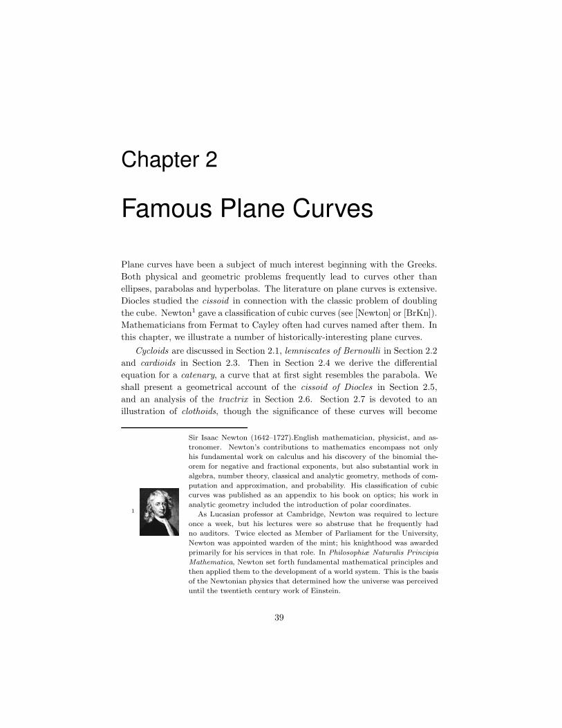
The general cycloid is defined by

cycloid[a, b](t) =(

at − b sin t, a − b cos t)

.

Taking a = b gives cycloid[a, a], which describes the locus of points traced by a

point on a circle of radius a which rolls without slipping along a straight line.

Figure 2.1: The cycloid t 7→ (t − sin t, 1 − cos t)

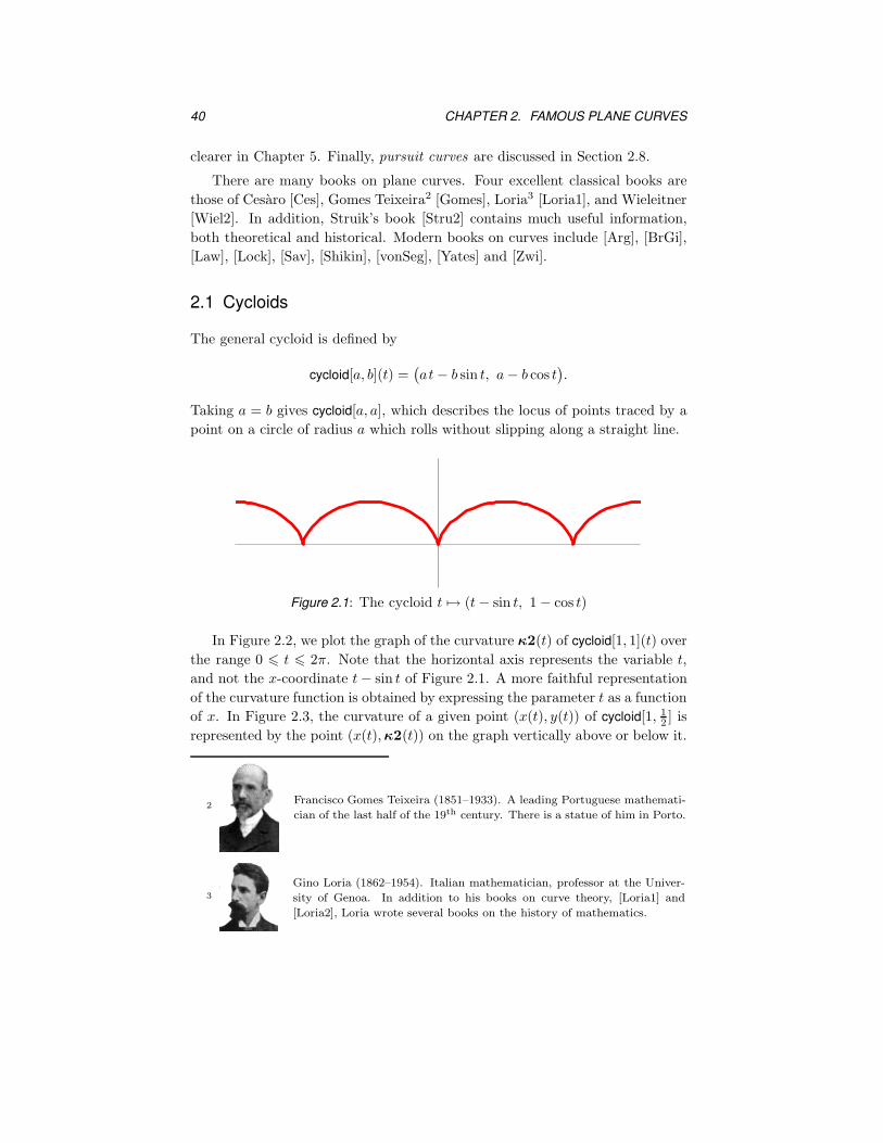
In Figure 2.2, we plot the graph of the curvature κ2(t) of cycloid[1, 1](t) over

the range 0 6 t 6 2π. Note that the horizontal axis represents the variable t,

and not the x-coordinate t − sin t of Figure 2.1. A more faithful representation

of the curvature function is obtained by expressing the parameter t as a function

of x. In Figure 2.3, the curvature of a given point (x(t), y(t)) of cycloid[1, 1

2] is

represented by the point (x(t), κ2(t)) on the graph vertically above or below it.

2Francisco Gomes Teixeira (1851–1933). A leading Portuguese mathemati-

cian of the last half of the 19th century. There is a statue of him in Porto.

3

Gino Loria (1862–1954). Italian mathematician, professor at the Univer-

sity of Genoa. In addition to his books on curve theory, [Loria1] and

[Loria2], Loria wrote several books on the history of mathematics.

2.1. CYCLOIDS 41

-1 1 2 3 4 5 6 7

-7

-6

-5

-4

-3

-2

-1

1

Figure 2.2: Curvature of cycloid[1, 1]

2 4 6

-2

-1

1

2

3

4

Figure 2.3: cycloid[1, 1

2] together with its curvature

Consider now the case in which a and b are not necessarily equal. The curve

cycloid[a, b] is that traced by a point on a circle of radius b when a concentric

circle of radius a rolls without slipping along a straight line. The cycloid is

prolate if a < b and curtate if a > b.

Figure 2.4: The prolate cycloid t 7→ (t − 3 sin t, 1 − 3 cos t)

42 CHAPTER 2. FAMOUS PLANE CURVES

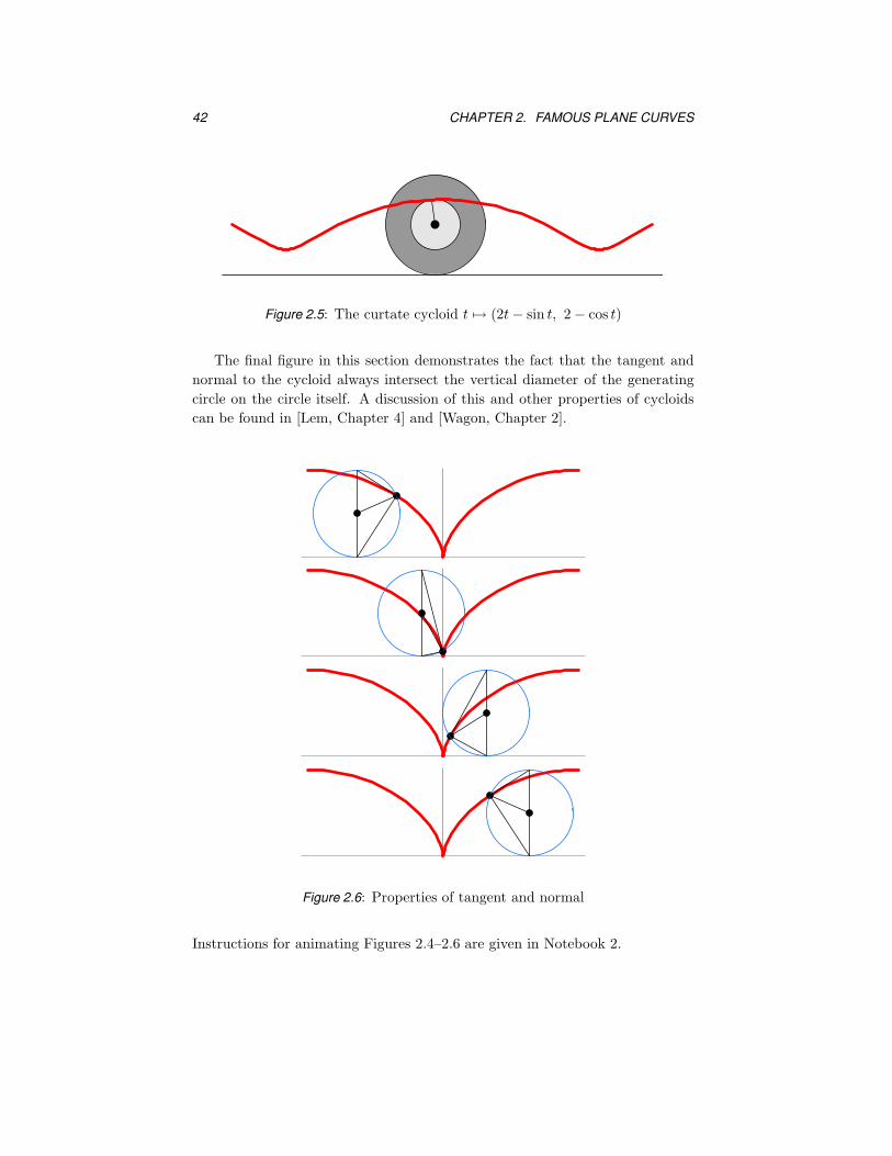
Figure 2.5: The curtate cycloid t 7→ (2t − sin t, 2 − cos t)

The final figure in this section demonstrates the fact that the tangent and

normal to the cycloid always intersect the vertical diameter of the generating

circle on the circle itself. A discussion of this and other properties of cycloids

can be found in [Lem, Chapter 4] and [Wagon, Chapter 2].

Figure 2.6: Properties of tangent and normal

Instructions for animating Figures 2.4–2.6 are given in Notebook 2.

2.2. LEMNISCATES OF BERNOULLI 43

2.2 Lemniscates of Bernoulli

Each curve in the family

lemniscate[a](t) =

(

a cos t

1 + sin2 t,

a sin t cos t

1 + sin2 t

)

,(2.1)

is called a lemniscate of Bernoulli4. Like an ellipse, a lemniscate has foci F1

and F2, but the lemniscate is the locus L of points P for which the product of

distances from F1 and F2 is a certain constant f2. More precisely,

L ={

(x, y) | distance(

(x, y), F1

)

distance(

(x, y), F2

)

= f2}

,

where distance(F1, F2) = 2f . This choice ensures that the midpoint of the

segment connecting F1 with F2 lies on the curve L .

Let us derive (2.1) from the focal property. Let the foci be (±f, 0) and let

L be a set of points containing (0, 0) such that the product of the distances

from F1 = (−f, 0) and F2 = (f, 0) is the same for all P ∈ L . Write P = (x, y).

Then the condition that P lie on L is

(

(x − f)2 + y2)(

(x + f)2 + y2)

= f4,(2.2)

or equivalently

(x2 + y2)2 = 2f2(x2 − y2).(2.3)

The substitutions y = x sin t, f = a/√

2 transform (2.3) into (2.1).

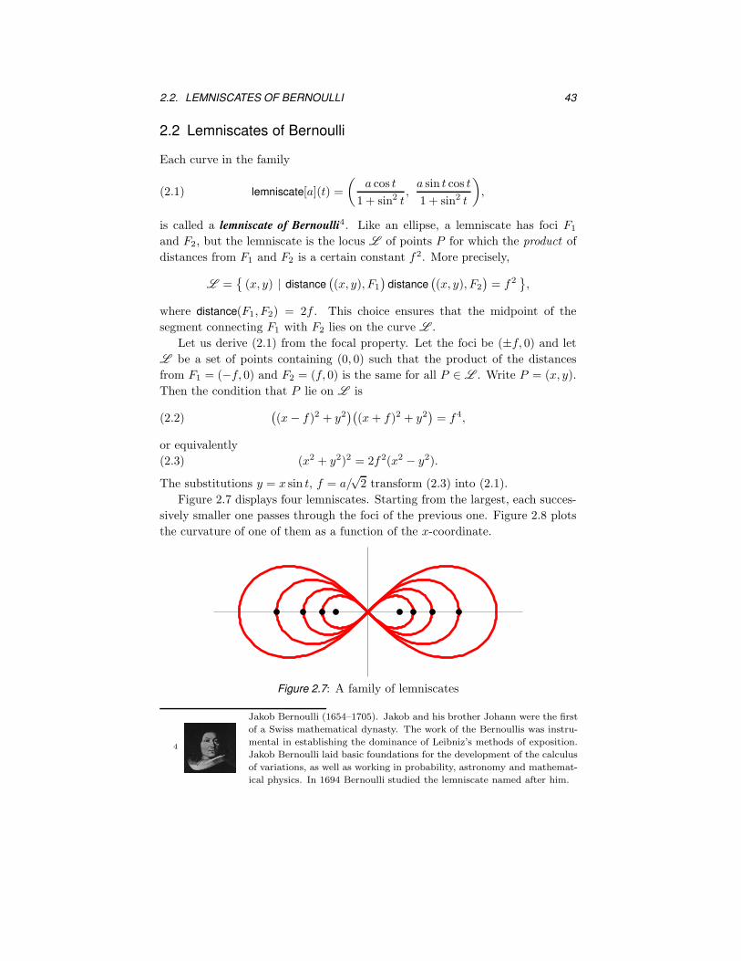
Figure 2.7 displays four lemniscates. Starting from the largest, each succes-

sively smaller one passes through the foci of the previous one. Figure 2.8 plots

the curvature of one of them as a function of the x-coordinate.

Figure 2.7: A family of lemniscates

4

Jakob Bernoulli (1654–1705). Jakob and his brother Johann were the first

of a Swiss mathematical dynasty. The work of the Bernoullis was instru-

mental in establishing the dominance of Leibniz’s methods of exposition.

Jakob Bernoulli laid basic foundations for the development of the calculus

of variations, as well as working in probability, astronomy and mathemat-

ical physics. In 1694 Bernoulli studied the lemniscate named after him.

44 CHAPTER 2. FAMOUS PLANE CURVES

Although a lemniscate of Bernoulli resembles the figure eight curve parame-

trized in the simper way by

eight[a](t) =(

sin t, sin t cos t)

,(2.4)

a comparison of the graphs of their respective curvatures shows the difference

between the two curves: the curvature of a lemniscate has only one maximum

and one minimum in the range 0 6 t < 2π, whereas (2.4) has three maxima,

three minima, and two inflection points.

-1 -0.5 0.5 1

-3

-2

-1

1

2

3

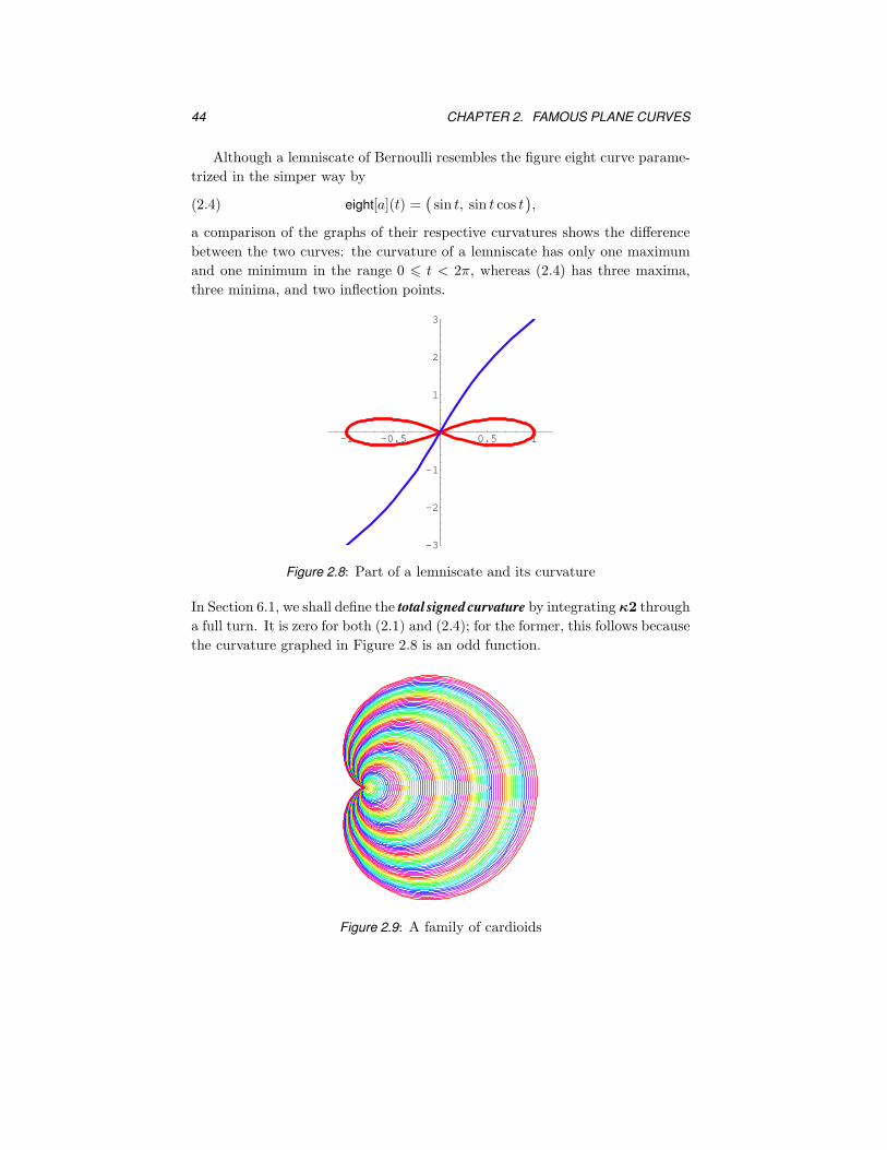
Figure 2.8: Part of a lemniscate and its curvature

In Section 6.1, we shall define the total signed curvature by integrating κ2 through

a full turn. It is zero for both (2.1) and (2.4); for the former, this follows because

the curvature graphed in Figure 2.8 is an odd function.

Figure 2.9: A family of cardioids

2.3. CARDIOIDS 45

2.3 Cardioids

A cardioid is the locus of points traced out by a point on a circle of radius a which

rolls without slipping on another circle of the same radius a. Its parametric

equation is

cardioid[a](t) =(

2a(1 + cos t) cos t, 2a(1 + cos t) sin t)

.

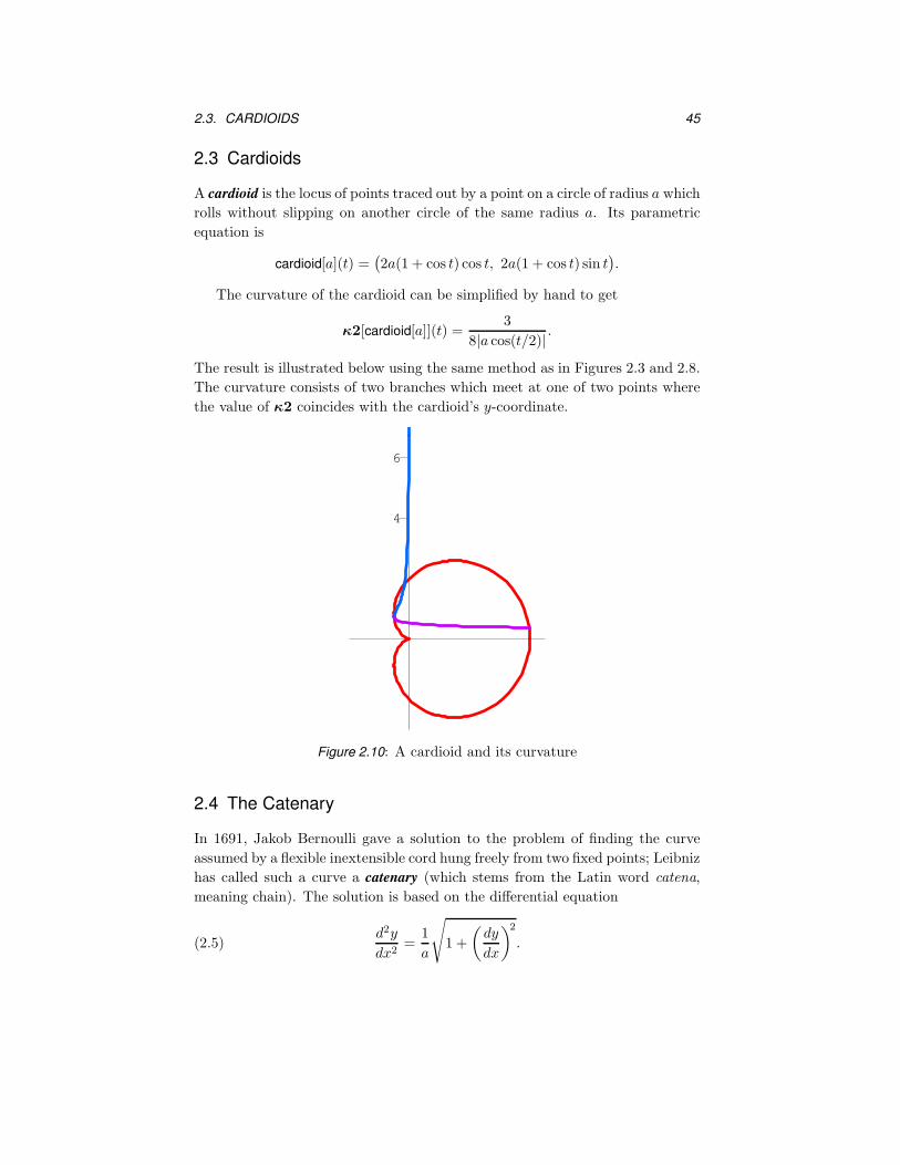
The curvature of the cardioid can be simplified by hand to get

κ2[cardioid[a]](t) =3

8|a cos(t/2)| .

The result is illustrated below using the same method as in Figures 2.3 and 2.8.

The curvature consists of two branches which meet at one of two points where

the value of κ2 coincides with the cardioid’s y-coordinate.

4

6

Figure 2.10: A cardioid and its curvature

2.4 The Catenary

In 1691, Jakob Bernoulli gave a solution to the problem of finding the curve

assumed by a flexible inextensible cord hung freely from two fixed points; Leibniz

has called such a curve a catenary (which stems from the Latin word catena,

meaning chain). The solution is based on the differential equation

d2y

dx2=

1

a

√

1 +

(

dy

dx

)2

.(2.5)

46 CHAPTER 2. FAMOUS PLANE CURVES

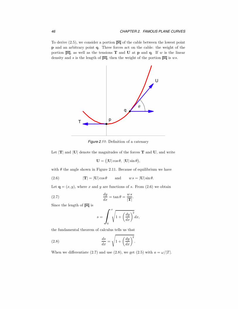
To derive (2.5), we consider a portion pq of the cable between the lowest point

p and an arbitrary point q. Three forces act on the cable: the weight of the

portion pq, as well as the tensions T and U at p and q. If w is the linear

density and s is the length of pq, then the weight of the portion pq is ws.

Θ

T

U

p

q

Figure 2.11: Definition of a catenary

Let |T| and |U| denote the magnitudes of the forces T and U, and write

U =(

|U| cos θ, |U| sin θ)

,

with θ the angle shown in Figure 2.11. Because of equilibrium we have

|T| = |U| cos θ and ws = |U| sin θ.(2.6)

Let q = (x, y), where x and y are functions of s. From (2.6) we obtain

dy

dx= tan θ =

ws

|T| .(2.7)

Since the length of pq is

s =

∫ x

0

√

1 +

(

dy

dx

)2

dx,

the fundamental theorem of calculus tells us that

ds

dx=

√

1 +

(

dy

dx

)2

.(2.8)

When we differentiate (2.7) and use (2.8), we get (2.5) with a = ω/|T |.

2.5. CISSOID OF DIOCLES 47

Although at first glance the catenary looks like a parabola, it is in fact the

graph of the hyperbolic cosine. A solution of (2.5) is given by

y = a coshx

a.(2.9)

The next figure compares a catenary and a parabola having the same curvature

at x = 0. The reader may need to refer to Notebook 2 to see which is which.

-4 -3 -2 -1 1 2 3 4

1

2

3

4

5

6

7

8

Figure 2.12: Catenary and parabola

We rotate the graph of (2.9) to define

catenary[a](t) =

(

a cosht

a, t

)

,(2.10)

where without loss of generality, we assume that a > 0. A catenary is one of

the few curves for which it is easy to compute the arc length function. Indeed,

|catenary[a]′(t)| = cosht

a,

and it follows that a unit-speed parametrization of a catenary is given by

s 7→ a

(√

1 +s2

a2, arcsinh

s

a

)

.

In Chapter 15, we shall use the catenary to construct an important minimal

surface called the catenoid.

2.5 The Cissoid of Diocles

The cissoid of Diocles is the curve defined nonparametrically by

x3 + xy2 − 2ay2 = 0.(2.11)

48 CHAPTER 2. FAMOUS PLANE CURVES

To find a parametrization of the cissoid, we substitute y = xt in (2.11) and

obtain

x =2at2

1 + t2, y =

2at3

1 + t2.

Thus we define

cissoid[a](t) =

(

2at2

1 + t2,

2at3

1 + t2

)

.(2.12)

The Greeks used the cissoid of Diocles to try to find solutions to the problems

of doubling a cube and trisecting an angle. For more historical information and

the definitions used by the Greeks and Newton see [BrKn, pages 9–12], [Gomes,

volume 1, pages 1–25] and [Lock, pages 130–133]. Cissoid means ‘ivy-shaped’.

Observe that cissoid[a]′(0) = 0 so that cissoid is not regular at 0. In fact, a

cissoid has a cusp at 0, as can be seen in Figure 2.14.

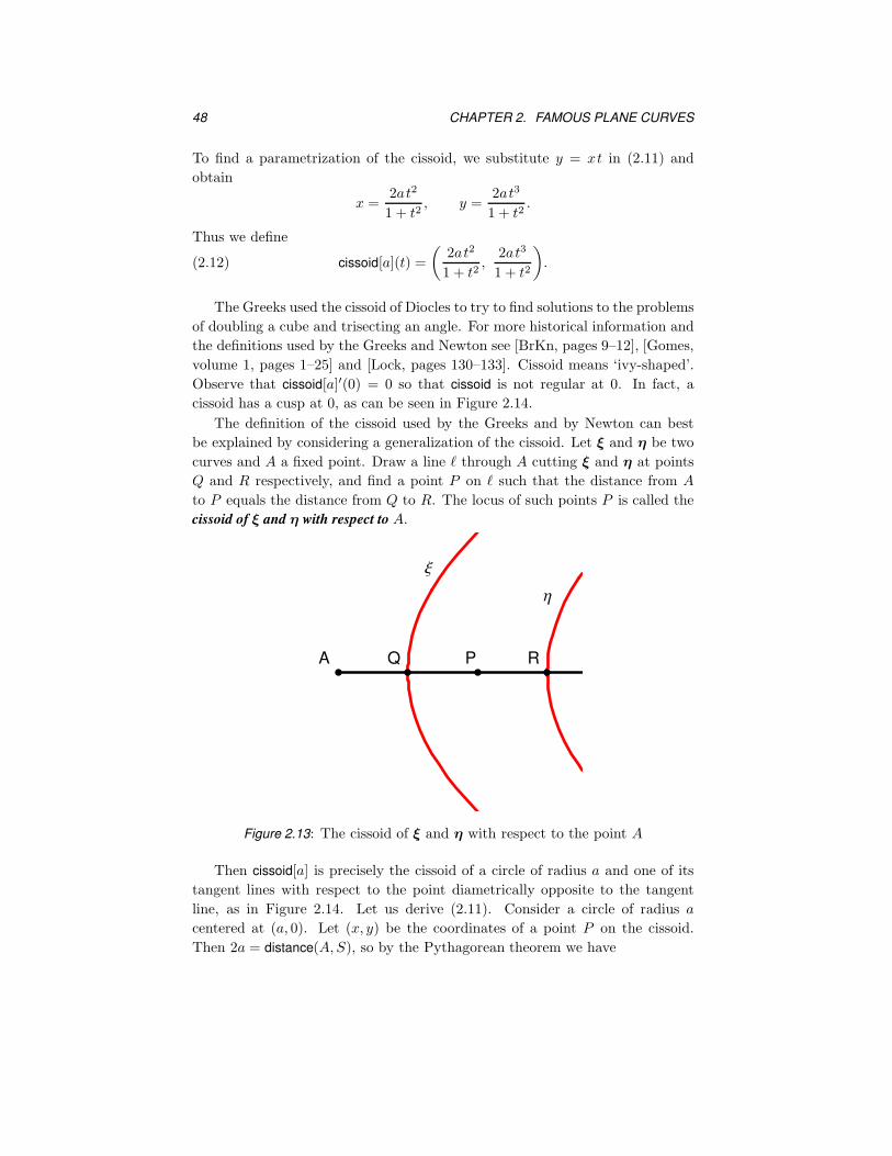
The definition of the cissoid used by the Greeks and by Newton can best

be explained by considering a generalization of the cissoid. Let ξ and η be two

curves and A a fixed point. Draw a line ` through A cutting ξ and η at points

Q and R respectively, and find a point P on ` such that the distance from A

to P equals the distance from Q to R. The locus of such points P is called the

cissoid of ξ and η with respect to A.

A Q P R

Ξ

Η

Figure 2.13: The cissoid of ξ and η with respect to the point A

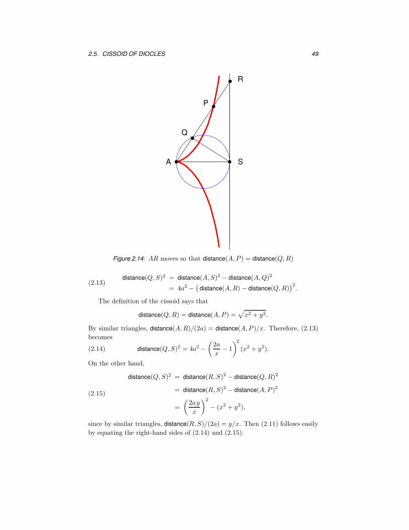
Then cissoid[a] is precisely the cissoid of a circle of radius a and one of its

tangent lines with respect to the point diametrically opposite to the tangent

line, as in Figure 2.14. Let us derive (2.11). Consider a circle of radius a

centered at (a, 0). Let (x, y) be the coordinates of a point P on the cissoid.

Then 2a = distance(A, S), so by the Pythagorean theorem we have

2.5. CISSOID OF DIOCLES 49

A

Q

P

R

S

Figure 2.14: AR moves so that distance(A, P ) = distance(Q, R)

distance(Q, S)2 = distance(A, S)2 − distance(A, Q)2

= 4a2 −(

distance(A, R) − distance(Q, R))2

.(2.13)

The definition of the cissoid says that

distance(Q, R) = distance(A, P ) =√

x2 + y2.

By similar triangles, distance(A, R)/(2a) = distance(A, P )/x. Therefore, (2.13)

becomes

distance(Q, S)2 = 4a2 −(

2a

x− 1

)2

(x2 + y2).(2.14)

On the other hand,

distance(Q, S)2 = distance(R, S)2 − distance(Q, R)2

= distance(R, S)2 − distance(A, P )2

=

(

2ay

x

)2

− (x2 + y2),

(2.15)

since by similar triangles, distance(R, S)/(2a) = y/x. Then (2.11) follows easily

by equating the right-hand sides of (2.14) and (2.15).

50 CHAPTER 2. FAMOUS PLANE CURVES

From Notebook 2, the curvature of the cissoid is given by

κ2[cissoid[a]](t) =3

a|t|(4 + t2)3/2,

and is everywhere strictly positive.

-1 -0.5 0.5 1

10

20

30

40

50

Figure 2.15: Curvature of the cissoid

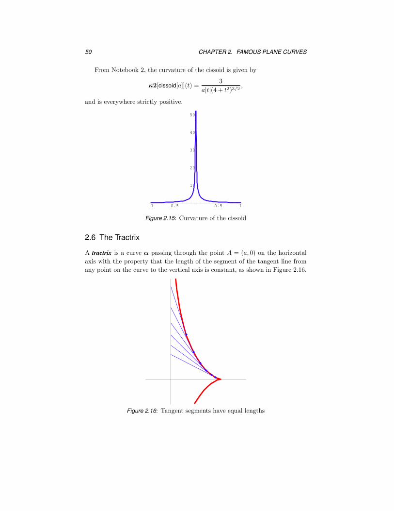
2.6 The Tractrix

A tractrix is a curve α passing through the point A = (a, 0) on the horizontal

axis with the property that the length of the segment of the tangent line from

any point on the curve to the vertical axis is constant, as shown in Figure 2.16.

Figure 2.16: Tangent segments have equal lengths

2.6. TRACTRIX 51

The German word for tractrix is the more descriptive Hundekurve. It is the

path that an obstinate dog takes when his master walks along a north-south

path. One way to parametrize the curve is by means of

tractrix[a](t) = a(

sin t, cos t + log(

tant

2

)

)

,(2.16)

It approaches the vertical axis asymptotically as t → 0 or t → π, and has a cusp

at t = π/2.

To find the differential equation of a tractrix, write tractrix[a](t) = (x(t), y(t)).

Then dy/dx is the slope of the curve, and the differential equation is therefore

dy

dx= −

√a2 − x2

x.(2.17)

It can be checked (with the help of (2.19) overleaf) that the differential equation

is satisfied by the components x(t) = a sin t and y(t) = a(

cos t + log(tan(t/2)))

of (2.16), and that both sides of (2.17) equal cot t.

Ha,0L

Hx,yL

x

a

Figure 2.17: Finding the differential equation

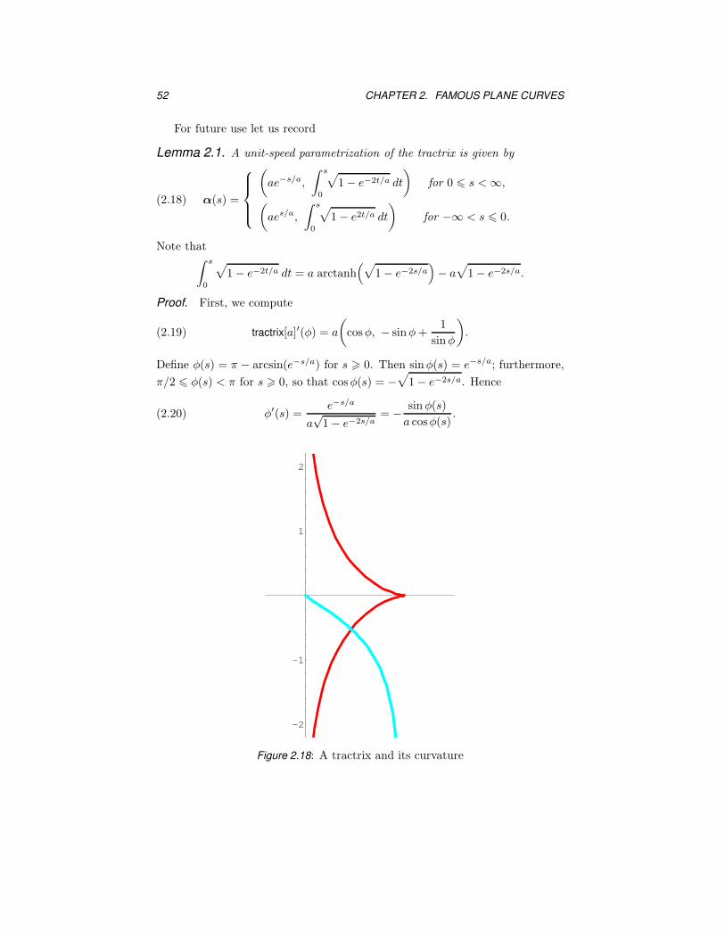
The curvature of the tractrix is

κ2[tractrix[1]](t) = −| tan t |.

In particular, it is everywhere negative and approaches −∞ at the cusp. Figure

2.18 graphs κ2 as a function of the x-coordinate sin t, so that the curvature at

a given point on the tractrix is found by referring to the point on the curvature

graph vertically below.

52 CHAPTER 2. FAMOUS PLANE CURVES

For future use let us record

Lemma 2.1. A unit-speed parametrization of the tractrix is given by

α(s) =

(

ae−s/a,

∫ s

0

√

1 − e−2t/a dt

)

for 0 6 s < ∞,

(

aes/a,

∫ s

0

√

1 − e2t/a dt

)

for −∞ < s 6 0.

(2.18)

Note that∫ s

0

√

1 − e−2t/a dt = a arctanh(√

1 − e−2s/a)

− a√

1 − e−2s/a.

Proof. First, we compute

tractrix[a]′(φ) = a

(

cosφ, − sin φ +1

sin φ

)

.(2.19)

Define φ(s) = π − arcsin(e−s/a) for s > 0. Then sinφ(s) = e−s/a; furthermore,

π/2 6 φ(s) < π for s > 0, so that cosφ(s) = −√

1 − e−2s/a. Hence

φ′(s) =e−s/a

a√

1 − e−2s/a= − sin φ(s)

a cosφ(s).(2.20)

-2

-1

1

2

Figure 2.18: A tractrix and its curvature

2.7. CLOTHOIDS 53

Therefore, if we define a curve β by β(s) = tractrix[a](

φ(s))

, it follows from

(2.19) and (2.20) that

β′(s) = tractrix[a]′(

φ(s))

φ′(s)

= a

(

cosφ(s),− sin φ(s) +1

sin φ(s)

)(

− sinφ(s)

a cosφ(s)

)

=(

− sin φ(s),− cosφ(s))

=(

−e−s/a,√

1 − e−2s/a)

= α′(s).

Also, β(0) = (a, 0) = α(0). Thus α and β coincide for 0 6 s < ∞, so that

α is a reparametrization of a tractrix in that range. The proof that α is a

reparametrization of tractrix[a] for −∞ < s 6 0 is similar. Finally, an easy

calculation shows that α has unit speed.

2.7 Clothoids

One of the most elegant of all plane curves is the clothoid or spiral of Cornu5.

We give a generalization of the clothoid by defining

clothoid[n, a](t) = a

(∫ t

0

sin

(

un+1

n + 1

)

du,

∫ t

0

cos

(

un+1

n + 1

)

du

)

.

Clothoids are important curves used in freeway and railroad construction (see

[Higg] and [Roth]). For example, a clothoid is needed to make the gradual

transition from a highway, which has zero curvature, to the midpoint of a freeway

exit, which has nonzero curvature. A clothoid is clearly preferable to a path

consisting of straight lines and circles, for which the curvature is discontinuous.

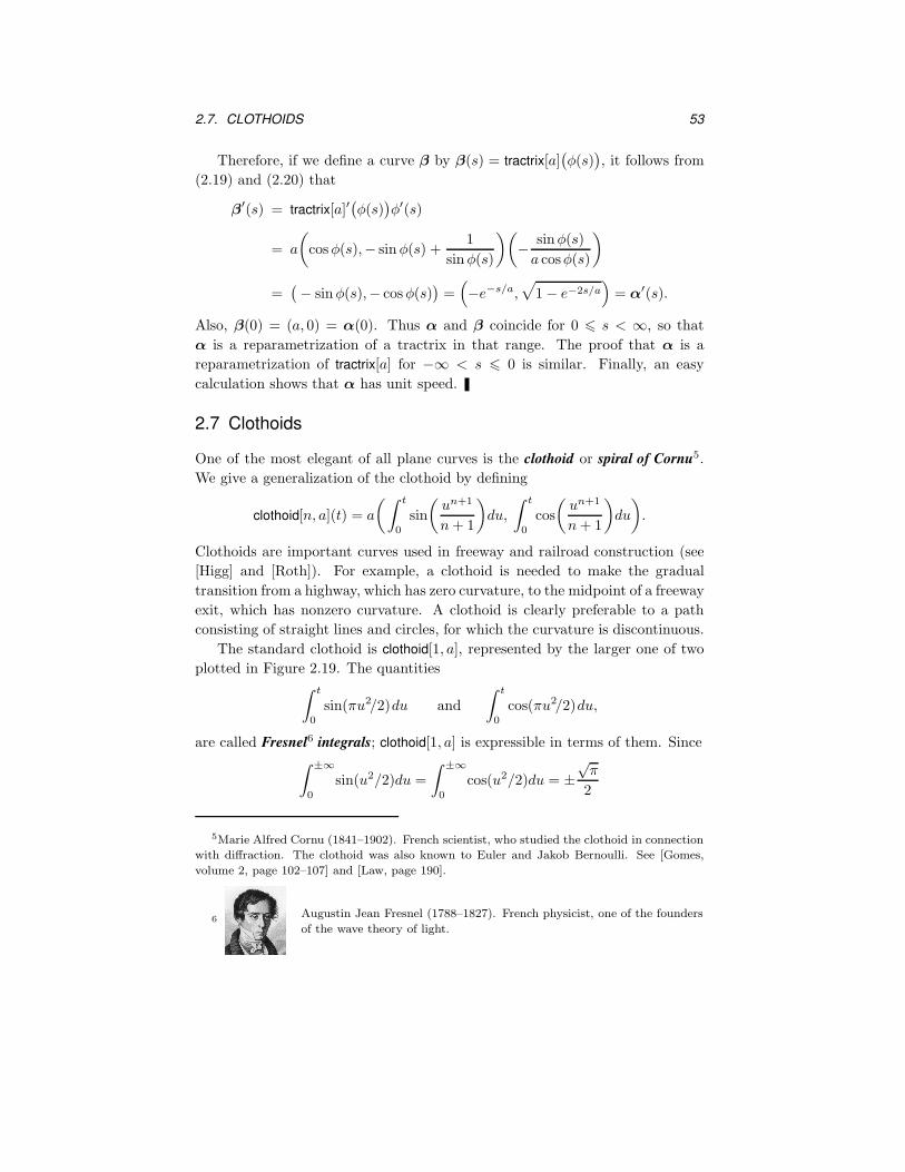
The standard clothoid is clothoid[1, a], represented by the larger one of two

plotted in Figure 2.19. The quantities∫ t

0

sin(πu2/2)du and

∫ t

0

cos(πu2/2)du,

are called Fresnel6 integrals; clothoid[1, a] is expressible in terms of them. Since∫ ±∞

0

sin(u2/2)du =

∫ ±∞

0

cos(u2/2)du = ±√

π

2

5Marie Alfred Cornu (1841–1902). French scientist, who studied the clothoid in connection

with diffraction. The clothoid was also known to Euler and Jakob Bernoulli. See [Gomes,

volume 2, page 102–107] and [Law, page 190].

6Augustin Jean Fresnel (1788–1827). French physicist, one of the founders

of the wave theory of light.

54 CHAPTER 2. FAMOUS PLANE CURVES

(as is easily checked by computer), the ends of the clothoid[1, a] curl around the

points ± 1

2a√

π(1, 1). The first clothoid is symmetric with respect to the origin,

but the second one (smaller in Figure 2.19) is symmetric with respect to the

horizontal axis. The odd clothoids have shapes similar to clothoid[1, a], while

the even clothoids have shapes similar to clothoid[2, a].

-1.5 -1 -0.5 0.5 1 1.5

-1.5

-1

-0.5

0.5

1

1.5

Figure 2.19: clothoid[1, 1] and clothoid[2, 1

2]

Although the definition of clothoid[n, a] is quite complicated, its curvature is

simple:

κ2[clothoid[n, a]](t) = − tn

a.(2.21)

In Chapter 5, we shall show how to define the clothoid as a numerical solution

to a differential equation arising from (2.21).

2.8 Pursuit Curves

The problem of pursuit probably originated with Leonardo da Vinci. It is to

find the curve by which a vessel moves while pursuing another vessel, supposing

that the speeds of the two vessels are always in the same ratio. Let us formulate

this problem mathematically.

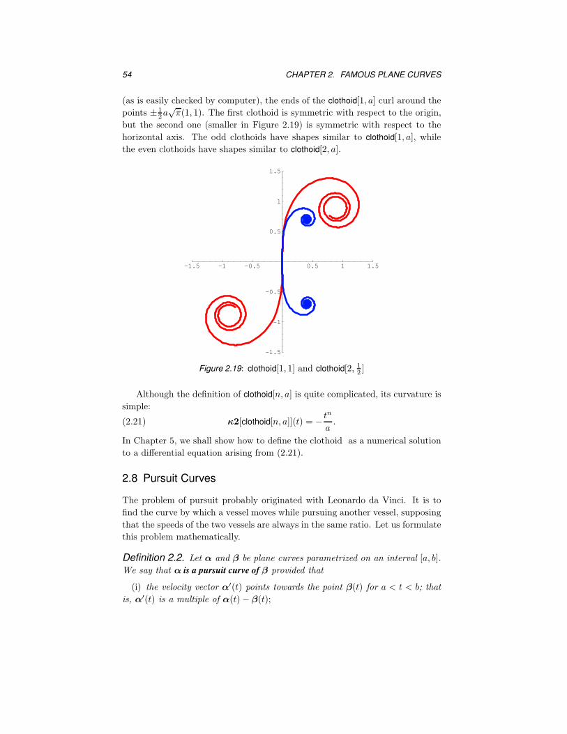
Definition 2.2. Let α and β be plane curves parametrized on an interval [a, b].

We say that α is a pursuit curve of β provided that

(i) the velocity vector α′(t) points towards the point β(t) for a < t < b; that

is, α′(t) is a multiple of α(t) − β(t);

2.8. PURSUIT CURVES 55

(ii) the speeds of α and β are related by ‖α′‖ = k‖β′‖, where k is a positive

constant. We call k the speed ratio.

A capture point is a point p for which p = α(t1) = β(t1) for some t1.

In Figure 2.20, α is the curve of the pursuer and β the curve of the pursued.

Β

Α

Figure 2.20: A pursuit curve

When the speed ratio k is larger than 1, the pursuer travels faster than the

pursued. Although this would usually be the case in a physical situation, it is

not a necessary assumption for the mathematical analysis of the problem.

We derive differential equations for pursuit curves in terms of coordinates.

Lemma 2.3. Write α = (x, y) and β = (f, g), and assume that α is a pursuit

curve of β. Then

x′2 + y′2 = k2(f ′2 + g′2)(2.22)

and

x′(y − g) − y′(x − f) = 0.(2.23)

Proof. Equation (2.22) is the same as ‖α′‖ = k‖β′‖. To prove (2.23), we

observe that α(t) − β(t) =(

x(t) − f(t), y(t) − g(t))

and α′(t) =(

x′(t), y′(t))

.

Note that the vector J(

α(t)−β(t))

=(

−y(t)+g(t), x(t)−f(t))

is perpendicular

to α(t)−β(t). The condition that α′(t) is a multiple of α(t)−β(t) is conveniently

expressed by saying that α′(t) is perpendicular to J(

α(t) − β(t))

, which is

equivalent to (2.23).

Next, we specialize to the case when the curve of the pursued is a straight

line. Assume that the curve β of the pursued is a vertical straight line passing

through the point (a, 0), and that the speed ratio k is larger than 1. We want

to find the curve α of the pursuer, assuming the initial conditions α(0) = (0, 0)

and α′(0) = (1, 0).

56 CHAPTER 2. FAMOUS PLANE CURVES

We can parametrize β as

β(t) =(

a, g(t))

.

Furthermore, the curve α of the pursuer can be parametrized as

α(t) =(

t, y(t))

.

The condition (2.22) becomes

1 + y′2 = k2g′2,(2.24)

and (2.23) reduces to

(y − g) − y′(t − a) = 0.

Differentiation with respect to t yields

−y′′(t − a) = g′.(2.25)

From (2.24) and (2.25) we get

1 + y′2 = k2(a − t)2y′′2.(2.26)

Let p = y′; then (2.26) can be rewritten as

k dp√

1 + p2=

dt

a − t.

This separable first-order equation has the solution

arcsinh p = −1

klog

(

a − t

a

)

,(2.27)

when we make use of the initial condition y′(0) = 0. Then (2.27) can be rewrit-

ten as

y′ = p = sinh(

arcsinh p)

= 1

2

(

earcsinh p − e−arcsinhp)

=1

2

(

(

a − t

a

)−1/k

−(

a − t

a

)1/k)

.

Integrating, with the initial condition y(0) = 0, yields

y =ak

k2 − 1+

1

2

(

ak

k + 1

(

a − t

a

)1+1/k

− ak

k − 1

(

a − t

a

)1−1/k)

.(2.28)

The curve of the pursuer is then α(t) = (t, y(t)), where y is given by (2.28).

Since α(t1) = β(t1) if and only if t1 = a, the capture point is

p =

(

a,ak

k2 − 1

)

.(2.29)

2.9. EXERCISES 57

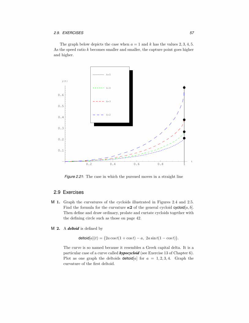
The graph below depicts the case when a = 1 and k has the values 2, 3, 4, 5.

As the speed ratio k becomes smaller and smaller, the capture point goes higher

and higher.

0.2 0.4 0.6 0.8 1t

0.1

0.2

0.3

0.4

0.5

0.6

yHtL

k=2

k=3

k=4

k=5

Figure 2.21: The case in which the pursued moves in a straight line

2.9 Exercises

M 1. Graph the curvatures of the cycloids illustrated in Figures 2.4 and 2.5.

Find the formula for the curvature κ2 of the general cycloid cycloid[a, b].

Then define and draw ordinary, prolate and curtate cycloids together with

the defining circle such as those on page 42.

M 2. A deltoid is defined by

deltoid[a](t) =(

2a cos t(1 + cos t) − a, 2a sin t(1 − cos t))

.

The curve is so named because it resembles a Greek capital delta. It is a

particular case of a curve called hypocycloid (see Exercise 13 of Chapter 6).

Plot as one graph the deltoids deltoid[a] for a = 1, 2, 3, 4. Graph the

curvature of the first deltoid.

58 CHAPTER 2. FAMOUS PLANE CURVES

M 3. The Lissajous7 or Bowditch curve8 is defined by

lissajous[n, d, a, b](t) =(

a sin(nt + d), b sin t)

.

Draw several of these curves and plot their curvatures. (One is shown in

Figure 11.19 on page 349.)

M 4. The limacon, sometimes called Pascal’s snail, named after Etienne Pascal,

father of Blaise Pascal9, is a generalization of the cardioid. It is defined

by

limacon[a, b](t) = (2a cos t + b)(

cos t, sin t)

.

Find the formula for the curvature of the limacon, and plot several of

them.

5. Consider a circle with center C = (0, a) and radius a. Let ` be the line tan-

gent to the circle at (0, 2a). A line from the origin O = (0, 0) intersecting `

at a point A intersects the circle at a point Q. Let x be the first coordinate

of A and y the second coordinate of Q, and put P = (x, y). As A varies

along ` the point P traces out a curve called versiera, in Italian and mis-

named in English as the witch of Agnesi10. Verify that a parametrization

of the Agnesi versiera is

agnesi[a](t) =(

2a tan t, 2a cos2 t)

.

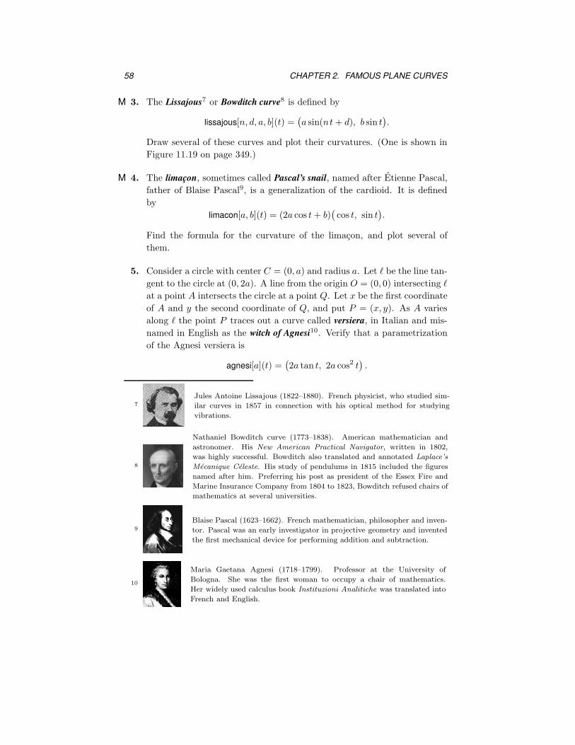
7

Jules Antoine Lissajous (1822–1880). French physicist, who studied sim-

ilar curves in 1857 in connection with his optical method for studying

vibrations.

8

Nathaniel Bowditch curve (1773–1838). American mathematician and

astronomer. His New American Practical Navigator, written in 1802,

was highly successful. Bowditch also translated and annotated Laplace’s

Mecanique Celeste. His study of pendulums in 1815 included the figures

named after him. Preferring his post as president of the Essex Fire and

Marine Insurance Company from 1804 to 1823, Bowditch refused chairs of

mathematics at several universities.

9

Blaise Pascal (1623–1662). French mathematician, philosopher and inven-

tor. Pascal was an early investigator in projective geometry and invented

the first mechanical device for performing addition and subtraction.

10

Maria Gaetana Agnesi (1718–1799). Professor at the University of

Bologna. She was the first woman to occupy a chair of mathematics.

Her widely used calculus book Instituzioni Analitiche was translated into

French and English.

2.9. EXERCISES 59

M 6. Define the curve

tschirnhausen[n, a](t) =

(

acos t

(cos(t/3))n, a

sin t

(cos(t/3))n

)

.

When n = 1, this curve is attributed to Tschirnhausen11. Find the formula

for the curvature of tschirnhausen[n, a][t] and make a simultaneous plot of

the curves for 1 6 n 6 8.

7. In the special case that the speed ratio is 1, show that the equation for

the pursuit curve is

y(t) =a

4

(

(

a − t

a

)2

− 1 − 2 log

(

a − t

a

)

)

,

and that the pursuer never catches the pursued.

M 8. Equation (2.28) defines the function

y(t) =ak

k2 − 1+

k(a − t)1+1/k

2a1/k(1 + k)− a1/kk(a − t)1−1/k

2(k − 1).

Plot a pursuit curve with a = 1 and k = 1.2.

11Ehrenfried Walter Tschirnhausen (1651–1708). German mathematician, who tried to

solve equations of any degree by removing all terms except the first and last. He contributed

to the rediscovery of the process for making hard-paste porcelain. Sometimes the name is

written von Tschirnhaus.