Asymptotic Curves and Geodesics on Surfaceswebmath2.unito.it/paginepersonali/sergio.console/Curve...Chapter 18 Asymptotic Curves and Geodesics on Surfaces In this chapter we begin

Chapter 18

Asymptotic Curves andGeodesics on Surfaces

In this chapter we begin a study of special curves lying on surfaces in R3. An

asymptotic curve on a surface M ⊂ R3 is a curve whose velocity always points

in a direction in which the normal curvature of M vanishes. In some sense, Mbends less along an asymptotic curve than it does along a general curve. As

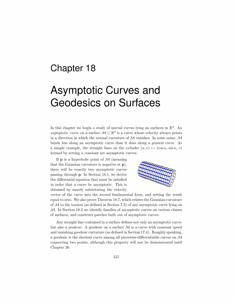
a simple example, the straight lines on the cylinder (u, v) 7→ (cosu, sinu, v)

formed by setting u constant are asymptotic curves.

If p is a hyperbolic point of M (meaning

that the Gaussian curvature is negative at p),

there will be exactly two asymptotic curves

passing through p. In Section 18.1, we derive

the differential equation that must be satisfied

in order that a curve be asymptotic. This is

obtained by merely substituting the velocity

vector of the curve into the second fundamental form, and setting the result

equal to zero. We also prove Theorem 18.7, which relates the Gaussian curvature

of M to the torsion (as defined in Section 7.2) of any asymptotic curve lying on

M. In Section 18.2 we identify families of asymptotic curves on various classes

of surfaces, and construct patches built out of asymptotic curves.

Any straight line contained in a surface defines not only an asymptotic curve,

but also a geodesic. A geodesic on a surface M is a curve with constant speed

and vanishing geodesic curvature (as defined in Section 17.4). Roughly speaking,

a geodesic is the shortest curve among all piecewise-differentiable curves on Mconnecting two points, although this property will not be demonstrated until

Chapter 26.

557

558 CHAPTER 18. ASYMPTOTIC CURVES AND GEODESICS

Geodesics were first studied by Johann Bernoulli1 in 1697, though the name

‘geodesic’ is due to Liouville in 1844. In Section 18.3, we determine the dif-

ferential equations for a geodesic. Their formulation allows one to prove that

there is a geodesic through a given point p pointing in any direction tangent

to M at p. This of course contrasts with the case of asymptotic curves, but is

what one expects intuitively from the distance-minimizing property of geodes-

ics. Many examples of parametrizations of surfaces that we have already given

in this book are so-called Clairaut patches, as defined in Section 18.5. These are

patches for which the geodesics equations simplify and are more readily solvable.

Applications are given in Section 18.6.

Since we shall be doing mostly local calculations in this chapter, we shall

assume that all surfaces are orientable, unless explicitly stated otherwise. This

means that we can choose once and for all a globally defined unit normal U for

any surface M.

18.1 Asymptotic Curves

Let M be a regular surface in R3. On page 390, we defined asymptotic directions

and asymptotic curves on a surface M. The former are defined by the vanishing

of the normal curvature at a given p ∈ M.

The following lemma is obvious from the definitions.

Lemma 18.1. Let M ⊂ R3 be a regular surface.

(i) At an elliptic point of M there are no asymptotic directions.

(ii) At a hyperbolic point of M there are exactly two asymptotic directions.

(iii) At a parabolic point of M there is exactly one asymptotic direction.

(iv) At a planar point of M every direction is asymptotic.

Hyperbolic points are considered in more detail in Theorem 18.4 below.

An asymptotic curve is a curve α in M for which the normal curvature

vanishes in the direction α′, that is

k(α′(t)

)= 0

1

Johann Bernoulli (1667–1748) occupied the chair of mathematics at

Groningen from 1695 to 1705, and at Basel, where he succeeded his el-

der brother Jakob, from 1705 to 1748. Although Johann was tutored

by Jakob, he became involved in controversies with him, and also with

his own son Daniel (1700–1782). Discoveries of Johann Bernoulli include

the exponential calculus, the treatment of trigonometry as a branch of

analysis, the determination of orthogonal trajectories and the solution of

the brachistochrone problem. Other mathematician sons of Johann were

Nicolaus (1695-1726) and Johann (II) (1710–1790).

18.1. ASYMPTOTIC CURVES 559

for all t in the domain of definition of α. Here is an alternative description.

Lemma 18.2. A curve α in a regular surface M ⊂ R3 is asymptotic if and

only if its acceleration α′′ is always tangent to M.

Proof. Without loss of generality, we can assume that α is a unit-speed curve.

If U denotes the surface normal to M, then differentiation of α′· U = 0 yields

0 = α′· U′ + α′′

· U = −k(α′) + α′′· U(18.1)

(see page 387). Hence k(α′) vanishes if and only if α′′ is perpendicular to U.

Next, we derive the differential equation for the asymptotic curves.

Lemma 18.3. Let α be a curve that lies in the image of a patch x. Write

α(t) = x(u(t), v(t)). Then α is an asymptotic curve if and only if one of the

following equivalent conditions is satisfied for all t:

(i) e(α(t)

)u′(t)2 + 2f

(α(t)

)u′(t)v′(t) + g

(α(t)

)v′(t)2 = 0;

(ii) II(α′(t),α′(t)

)= 0, where II is the second fundamental form defined on

page 401.

Proof. Corollary 10.15, page 294, implies that α′ = xuu′ + xvv

′. Hence by

Lemma 13.17 on page 395, we have

k(α′(t)

)=

e(α(t)

)u′(t)2 + 2f

(α(t)

)u′(t)v′(t) + g

(α(t)

)v′(t)2

E(α(t)

)u′(t)2 + 2F

(α(t)

)u′(t)v′(t) +G

(α(t)

)v′(t)2

.(18.2)

Then (i) follows from (18.2), and (ii) is a restatement of (i).

The equation in (i) can be written more succinctly as

eu′2 + 2f u′v′ + gv′2 = 0.(18.3)

We call (18.3) the differential equation for the asymptotic curves of a surface.

Using Lemma 13.31 on page 405, we see that (18.3) is equivalent to

eu′2 + 2fu′v′ + gv′2 = 0,(18.4)

in terms of the triple products

e = [xuu xu xv], f = [xuv xu xv], g = [xvv xu xv].

Theorem 18.4. In a neighborhood of a hyperbolic point p of a regular surface

M ⊂ R3 there exist two distinct families of asymptotic curves.


Proof. In a neighborhood of a hyperbolic point p, the equation

ea2 + 2f ab+ g b2 = 0

has real roots. Hence we have the factorization

ea2 + 2f ab+ g b2 = (Aa+Bb)(Ca+Db),

where A,B,C,D are real. Thus the differential equation for the asymptotic

curves also factors:

(Au′ +Bv′)(Cu′ +Dv′) = 0,(18.5)

where now A,B,C,D are real functions. One family consists of the solution

curves to Au′ +Bv′ = 0, and the other family consists of the solution curves to

Cu′ +Dv′ = 0.

Next, we give a characterization of an asymptotic curve in terms of its cur-

vature as a curve in R3.

Theorem 18.5. Let α be a regular curve on a regular surface M ⊂ R3, and

denote by {T,B,N} the Frenet frame and by κ[α] the curvature of α. Also, let

U be the surface normal of M. Then α is an asymptotic curve if and only if at

every point α(t), either κ[α](t) = 0 or N(t) · U = 0.

Proof. Without loss of generality, we can assume that α has unit speed. The

first Frenet formula (see page 197) in the case of nonzero curvature κ[α] is

T′ = κ[α]N.(18.6)

We can also make sense of (18.6) at points where κ[α] vanishes, by choosing

the unit vector N arbitrarily. By (18.1), we have

k(α′) = α′′· U = T′

· U = κ[α]N · U.

It follows that at each point α(t), either κ[α] = 0 or N is well defined and

perpendicular to U. The conclusion follows.

The curvature of a straight line vanishes identically, whence

Corollary 18.6. A straight line that is contained in a regular surface is neces-

sarily an asymptotic curve.

Now we establish an important relation between the torsion of an asymptotic

curve and the Gaussian curvature of the surface containing it.

18.1. ASYMPTOTIC CURVES 561

Theorem 18.7. (Beltrami2-Enneper) Let α be an asymptotic curve on a regu-

lar surface M ⊂ R3, and assume the curvature κ[α] of α does not vanish. Then

the torsion τ [α] of α and the Gaussian curvature K of M are related along α

by

K ◦ α = −τ [α]2.

Proof. Without loss of generality, we can assume that α is a unit-speed curve.

Since α is an asymptotic curve with nonvanishing curvature, it follows from

Theorem 18.5 that

T · U = N · U = 0.

Therefore, U = ±B along α. Then the third Frenet formula of (7.12) implies

that

τ [α]2 = B′· B′ =

dU

ds· dUds

.(18.7)

On the other hand, since the second fundamental form II of M vanishes along

α, equation (13.23), page 402, for the third fundamental form reduces to

0 = (III +K I)(α′,α′) =dU

ds·

dU

ds+K.(18.8)

The theorem follows from (18.7) and (18.8).

Corollary 18.8. An asymptotic curve on a regular surface M ⊂ R3 with con-

stant negative curvature has constant torsion.

This result applies in particular to the examples of surfaces given in Sections 15.4

and 15.6.

Next, we consider the problem of building patches from asymptotic curves.

Definition 18.9. An asymptotic patch on a regular surface M ⊂ R3 is a patch

for which the u- and v-parameter curves are asymptotic curves.

Theorem 18.10. Let x be a patch for which f never vanishes. Then x is an

asymptotic patch if and only if e and g vanish identically.

2

Eugenio Beltrami (1835–1900). Professor at the Universities of Bologna,

Pisa, Padua and Rome. He found the first concrete model of non-Euclidean

geometry, published in [Beltr] and in this paper showed how possible

contradictions in non-Euclidean geometry would reveal themselves in the

Euclidean geometry of surfaces. Beltrami also made known the work of

the Jesuit mathematician Saccheri, whose work Euclides ab omni naevo

vindicatus foreshadowed non-Euclidean geometry.


Proof. If the curve u 7→ x(u, v) is asymptotic, it follows from Lemma 18.2 that

e = xuu · U = 0. Similarly, if v 7→ x(u, v) is asymptotic, then g = 0. Conversely,

if e and g vanish identically, the differential equation for the asymptotic curves

becomes

f u′v′ = 0.

Clearly, u = u0 and v = v0 are solutions of this differential equation. Otherwise

said, the u- and v-parameter curves are asymptotic.

18.2 Examples of Asymptotic Curves and Patches

Ruled surfaces

According to Corollary 18.6, ruled surfaces are constructed from asymptotic

straight lines. For example, if we parametrize the hyperbolic paraboloid z = xy

by (10.12), page 296, it is easy to compute e = g = 0 and f = (1+u2 + v2)−1/2.

Hence, by Theorem 18.10, (u, v) 7→ (u, v, uv) is an asymptotic patch. Of course

the resulting curves

u 7→ (u, v0, uv0) and v 7→ (u0, v, u0v)

are the straight-line rulings visible in Figure 14.3 on page 435.

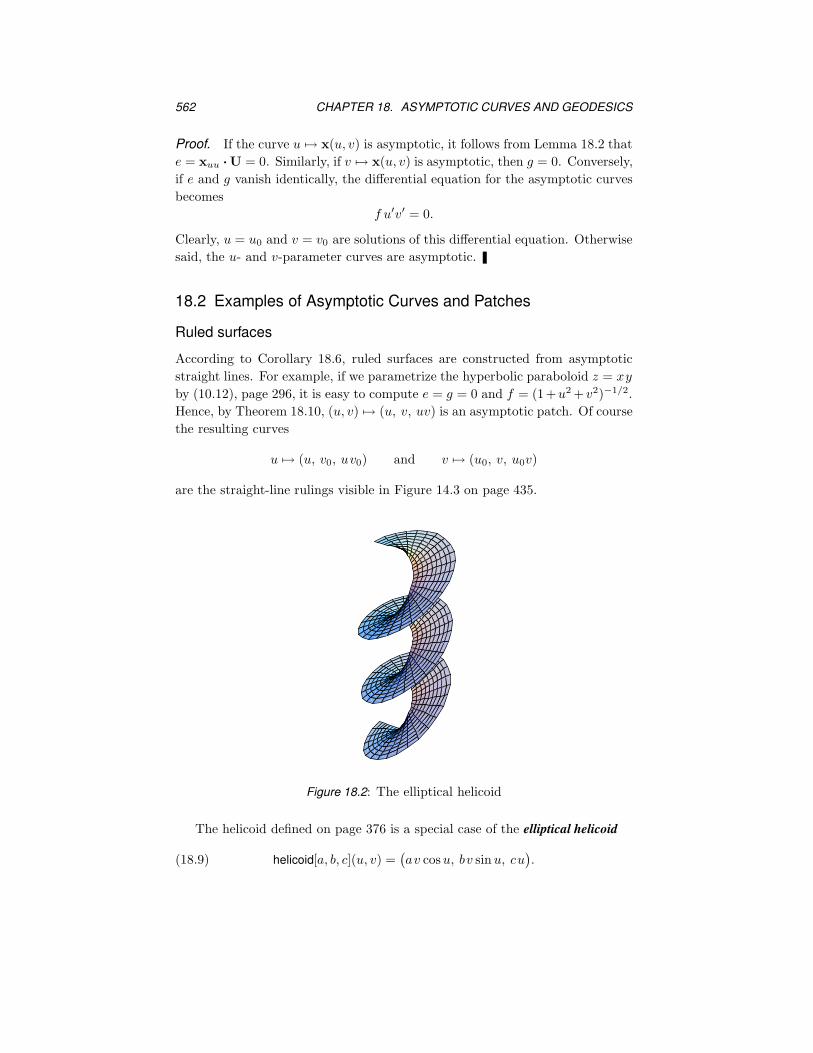
Figure 18.2: The elliptical helicoid

The helicoid defined on page 376 is a special case of the elliptical helicoid

helicoid[a, b, c](u, v) =(av cosu, bv sinu, cu

).(18.9)

18.2. EXAMPLES OF ASYMPTOTIC CURVES 563

Like the previous example, helicoid[a, b, c] is an asymptotic patch, but this time

only the v-parameter curves are straight lines. The u-parameter curves are, of

course, elliptical helices. Theorem 18.7 tells us that the Gaussian curvature of

the elliptical helicoid, when restricted to one of these helices, equals minus the

square of the torsion of the helix. This fact is verified in Notebook 18.

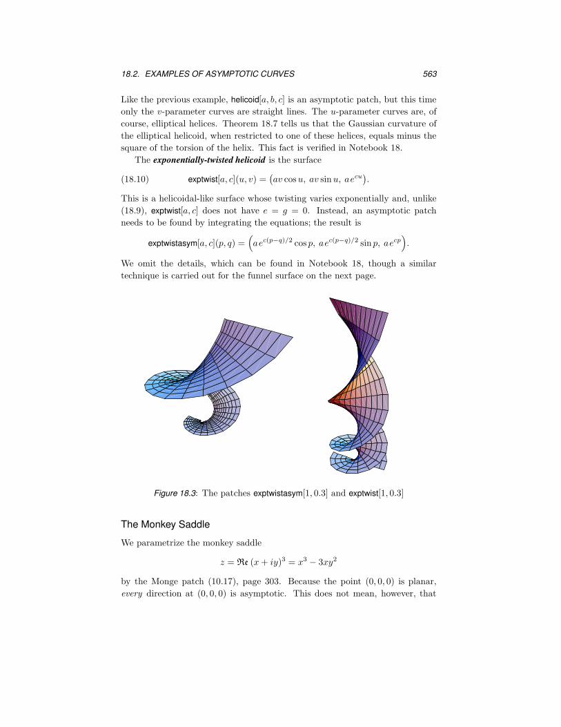
The exponentiallytwisted helicoid is the surface

exptwist[a, c](u, v) =(av cosu, av sinu, aecu

).(18.10)

This is a helicoidal-like surface whose twisting varies exponentially and, unlike

(18.9), exptwist[a, c] does not have e = g = 0. Instead, an asymptotic patch

needs to be found by integrating the equations; the result is

exptwistasym[a, c](p, q) =(aec(p−q)/2 cos p, aec(p−q)/2 sin p, aecp

).

We omit the details, which can be found in Notebook 18, though a similar

technique is carried out for the funnel surface on the next page.

Figure 18.3: The patches exptwistasym[1, 0.3] and exptwist[1, 0.3]

The Monkey Saddle

We parametrize the monkey saddle

z = Re (x+ iy)3 = x3 − 3xy2

by the Monge patch (10.17), page 303. Because the point (0, 0, 0) is planar,

every direction at (0, 0, 0) is asymptotic. This does not mean, however, that


there are asymptotic curves in every direction. But it is easy to find three

straight lines passing through (0, 0, 0) that lie entirely in the surface, namely

v 7→ (0, v, 0),

v 7→ (v√

3, v, 0),

v 7→ (−v√

3, v, 0).

Independently, it can be checked that each of these curves satisfies the differen-

tial equation

uu′2 − 2vu′v′ − uv′2 = 0

for asymptotic curves. These three lines are also examples of geodesics, and

have been emphasized as such in Figure 18.5.

The Funnel Surface

Consider the regular surface which is the image of the patch

x : (0,∞) × [0, 2π] −→ R3

x(r, θ) = (r cos θ, r sin θ, log r).(18.11)

This is a parametrization of the graph of the function

z =1

2log(x2 + y2).

We compute

e =−1

r√

1 + r2, f = 0, g =

r√1 + r2

.

Thus the differential equation for the asymptotic curves becomes

−r′2

r+ rθ′2 = 0, or θ′ = ±r

′

r.(18.12)

The two equations θ′ = ±r′/r have respective solutions

θ + 2u = log r, θ + 2v = − log r,

where u and v are constants of integration. Solving for r and θ in terms of u

and v gives

r = eu−v and θ = −u− v.

The patch

y(u, v) = x(r(u, v), θ(u, v)

)

=(eu−v cos(u+ v), −eu−v sin(u + v), u− v

)

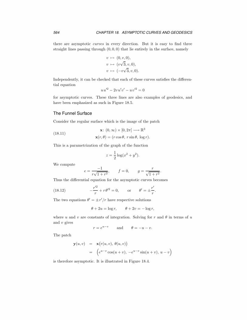
is therefore asymptotic. It is illustrated in Figure 18.4.

18.3. GEODESIC EQUATIONS 565

Figure 18.4: The funnel surface with asymptotic patch

18.3 The Geodesic Equations

Our starting point is the following definition of a geodesic on a surface in R3.

Definition 18.11. Let M ⊂ R3 be a surface and α : (a, b) → M a curve. We

say that α is a geodesic on M if the tangential component α′′(t)> of the accel-

eration of α vanishes.

It is important to note that we do not assume that α has unit speed in this

definition. Nonetheless,

Lemma 18.12. A geodesic α necessarily has constant speed.

Proof. We computed

dt‖α′(t)‖2 = 2α′′(t) · α′(t).

Since α′(t) is tangential to the surface, the right-hand side is zero, and

ds

dt= ‖α′(t)‖

is constant.

The definition of geodesic is in some sense complementary to that of asymp-

totic curve. Recall (see page 390) that α : (a, b) → M ⊂ R3 is an asymptotic

curve provided the normal component of α′′ vanishes. However, there is an

important difference, since the definition of geodesic requires no knowledge of


normal directions, and immediately extends to a surface in Rn. Indeed, we shall

soon see that geodesics can be defined instrinsically, in terms of just the first

fundamental form.

The following result is an immediate consequence of Theorem 17.7 on page 539,

and an analogue of Corollary 18.6.

Corollary 18.13. A straight line in R3 that is contained in a surface M is a

geodesic on M, provided its parametrization has constant speed.

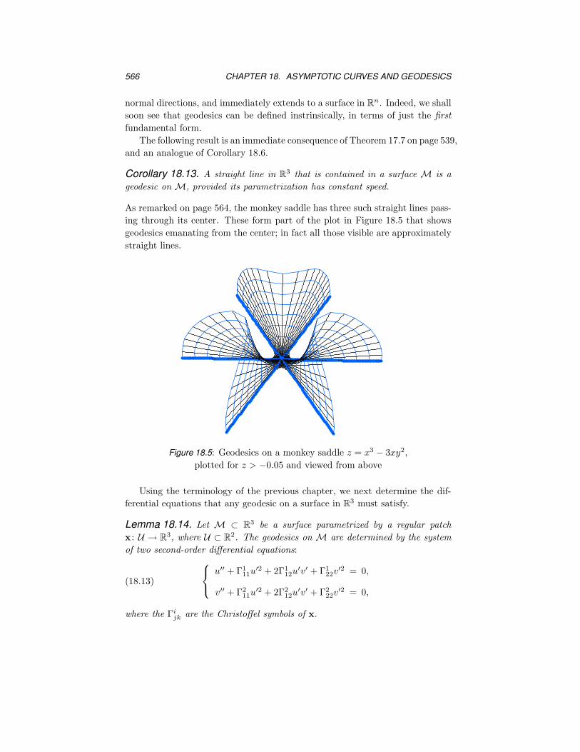
As remarked on page 564, the monkey saddle has three such straight lines pass-

ing through its center. These form part of the plot in Figure 18.5 that shows

geodesics emanating from the center; in fact all those visible are approximately

straight lines.

Figure 18.5: Geodesics on a monkey saddle z = x3 − 3xy2,

plotted for z > −0.05 and viewed from above

Using the terminology of the previous chapter, we next determine the dif-

ferential equations that any geodesic on a surface in R3 must satisfy.

Lemma 18.14. Let M ⊂ R3 be a surface parametrized by a regular patch

x : U → R3, where U ⊂ R

2. The geodesics on M are determined by the system

of two second-order differential equations:

u′′ + Γ111u

′2 + 2Γ112u

′v′ + Γ122v

′2 = 0,

v′′ + Γ211u

′2 + 2Γ212u

′v′ + Γ222v

′2 = 0,(18.13)

where the Γijk are the Christoffel symbols of x.

18.3. GEODESIC EQUATIONS 567

Proof. Let α : (a, b) → M be a curve. We can write

α(t) = x(u(t), v(t)

),(18.14)

where u, v : (a, b) → R are differentiable functions. When we differentiate (18.14)

twice using the chain rule, we get

α′′ = xuuu′2 + xuu

′′ + 2xuvu′v′ + xvvv

′2 + xvv′′.(18.15)

Then (17.8), page 538, and (18.15) imply that

α′′(t) =(u′′ + Γ1

11u′2 + 2Γ1

12u′v′ + Γ1

22v′2

)xu

+(v′′ + Γ2

11u′2 + 2Γ2

12u′v′ + Γ2

22v′2

)xv

+(eu′2 + 2f u′v′ + gv′2

)U,

(18.16)

where

U =xu × xv

‖xu × xv‖is the unit normal vector field to M. In order that α be a geodesic, the coeffi-

cients of xu and xv in (18.16) must each vanish. Hence we get (18.13).

Now we can obtain another important property of geodesics.

Corollary 18.15. Isometries and local isometries preserve geodesics.

Proof. Since the Christoffel symbols are expressible in terms of E, F and G,

Corollary 12.8 implies that local isometries preserve equations (18.13).

Next, we prove that from each point on a surface there is a geodesic in every

direction. More precisely:

Theorem 18.16. Let p be a point on a surface M and vp a tangent vector to

M at p. Then there exists a geodesic γ parametrized on some interval contain-

ing 0 such that γ(0) = p and γ′(0) = vp. Furthermore, any two geodesics with

these initial conditions coincide on any interval containing 0 on which they are

defined.

Proof. Let x : U → M be a regular patch with x(0, 0) = p. Then (18.13) is

the system of differential equations determining the geodesics on the trace of x.

Writing γ(t) = x(u(t), v(t)), the initial conditions translate into{

u(0) = 0,

v(0) = 0,and

{u′(0) = v1,

v′(0) = v2,(18.17)

where v1, v2 are the components of vp. From the theory of ordinary differential

equations, we know that the system (18.13) together with the four initial con-

ditions (18.17) has a unique solution on some interval containing 0. Hence the

theorem follows.


Theorem 18.16 gives no information concerning the size of the interval on

which the geodesic satisfying given initial conditions is defined. Let γ1 and γ2

be geodesics satisfying the same initial conditions. Since the two geodesics must

coincide on some interval, it is clear that there is a geodesic γ3 whose domain

of definition contains those of both γ1 and γ2 and coincides wherever possible

with the two geodesics. Applying this consistency result, we obtain a single

maximal geodesic. The domain of a maximal geodesic may or may not be the

whole real line, and we shall discuss this matter further in Chapter 26.

It is important to distinguish between a geodesic and the trace of a geo-

desic, because not every reparametrization of a geodesic has constant speed.

Therefore, we introduce the following notion:

Definition 18.17. A curve α in a surface M is called a pregeodesic provided

there is a reparametrization α ◦ h of α such that α ◦ h is a geodesic.

We can now characterize a pregeodesic by the vanishing of the geodesic curva-

ture, defined in Section 17.4. See also Exercise 11.

Lemma 18.18. Let M be a surface and let α : (a, b) → M be a regular curve.

Then the following conditions are equivalent:

(i) α is a pregeodesic;

(ii) there exists a function f : (a, b) → R such that

α′′(t)> = f(t)α′(t)

for a < t < b;

(iii) the geodesic curvature of α vanishes.

Proof. Suppose β = α ◦ h is a geodesic. Without loss of generality, β′ never

vanishes. Then β′ = (α′ ◦ h)h′, so that h′ never vanishes. Furthermore, it

follows that

0 = (β′′)> = h′2(α′′ ◦ h)> + h′′(α′ ◦ h),so that

(α′′)> = −(h′′

h′2◦ h−1

)α′;

thus we can take f = −(h′′/h′2) ◦ h−1.

Conversely, assume that (α′′)> = fα′ and let h be a nonzero solution of the

differential equation h′′ + h′2(f ◦ h) = 0. Put β = α ◦ h; then

(β′′)> = h′2(α′′ ◦ h)> + h′′(α′ ◦ h) =((f ◦ h)h′2 + h′′

)α′ ◦ h = 0.

This establishes the equivalence of (i) and (ii).

The equivalence of (ii) and (iii) follows from equation (17.18) on page 542.

For κg[α] vanishes if and only if α′′(t) · Jα(t)′ = 0 for all t, which is equivalent

to (ii).

18.4. FIRST EXAMPLES OF GEODESICS 569

18.4 First Examples of Geodesics

We begin with a general result relating the shape operator of a surface in R3

and the Frenet frame of a curve on the surface.

Lemma 18.19. Let M be an orientable surface in R3, and let α : (a, b) → M

be a unit-speed geodesic on M with nonzero curvature. Denote by {T,N,B} the

Frenet frame field of α and by κ and τ the curvature and torsion of α. Then

it is possible to choose a unit normal vector field U to M such that

S(T) = κT − τ B,(18.18)

where S denotes the shape operator of M with respect to U.

Proof. Since α has nonzero curvature, the vector field N is defined on all

of (a, b). The assumption that α is a geodesic implies that N = α′′/κ2 is

everywhere perpendicular to M. Thus it is possible to choose U so that

N(t) = U(α(t)

)

for a < t < b. By the definition of the shape operator and by the Frenet

Formulas (7.12), page 197, we have

S(T) = − d

dtU

(α(t)

)= −N′ = κT − τ B.

Before proceeding further with the general theory, we find geodesics in three

important cases.

Geodesics on a Sphere

We can use Lemma 18.19 to determine the geodesics of a sphere.

Lemma 18.20. The geodesics on a sphere of radius c > 0 in R3 are parts of

great circles.

Proof. Let β be a geodesic on a sphere of radius c. By part (i) of Theorem 8.15,

page 242, the curvature of β is nonzero, so that the Frenet frame {T,N,B} of

β is well defined. Since the principal curvatures of a sphere are constant and

equal, the shape operator of the sphere (with a proper choice of the unit normal)

satisfies

S(T) =1

cT.(18.19)

It follows from (18.18) and (18.19) that the curvature of β has the constant

value 1/c, and that the torsion vanishes. Moreover, part (vi) of Theorem 8.15

implies that β is part of a circle. Since the radius of the circle is the maximum

possible, β must be part of a great circle.


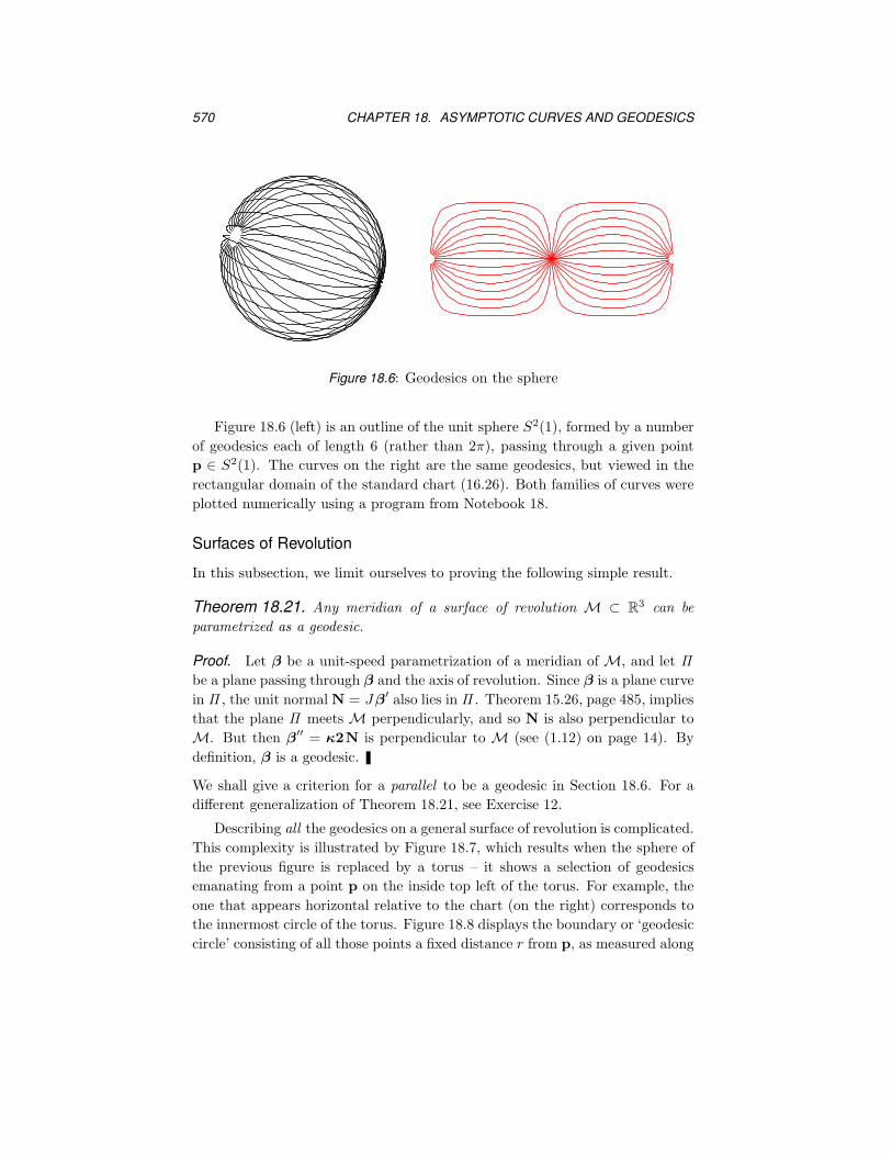
Figure 18.6: Geodesics on the sphere

Figure 18.6 (left) is an outline of the unit sphere S2(1), formed by a number

of geodesics each of length 6 (rather than 2π), passing through a given point

p ∈ S2(1). The curves on the right are the same geodesics, but viewed in the

rectangular domain of the standard chart (16.26). Both families of curves were

plotted numerically using a program from Notebook 18.

Surfaces of Revolution

In this subsection, we limit ourselves to proving the following simple result.

Theorem 18.21. Any meridian of a surface of revolution M ⊂ R3 can be

parametrized as a geodesic.

Proof. Let β be a unit-speed parametrization of a meridian of M, and let Π

be a plane passing through β and the axis of revolution. Since β is a plane curve

in Π , the unit normal N = Jβ′ also lies in Π . Theorem 15.26, page 485, implies

that the plane Π meets M perpendicularly, and so N is also perpendicular to

M. But then β′′ = κ2N is perpendicular to M (see (1.12) on page 14). By

definition, β is a geodesic.

We shall give a criterion for a parallel to be a geodesic in Section 18.6. For a

different generalization of Theorem 18.21, see Exercise 12.

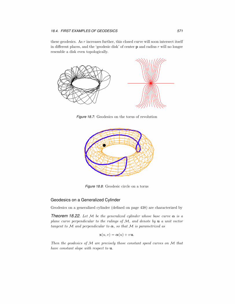
Describing all the geodesics on a general surface of revolution is complicated.

This complexity is illustrated by Figure 18.7, which results when the sphere of

the previous figure is replaced by a torus – it shows a selection of geodesics

emanating from a point p on the inside top left of the torus. For example, the

one that appears horizontal relative to the chart (on the right) corresponds to

the innermost circle of the torus. Figure 18.8 displays the boundary or ‘geodesic

circle’ consisting of all those points a fixed distance r from p, as measured along

18.4. FIRST EXAMPLES OF GEODESICS 571

these geodesics. As r increases further, this closed curve will soon intersect itself

in different places, and the ‘geodesic disk’ of center p and radius r will no longer

resemble a disk even topologically.

Figure 18.7: Geodesics on the torus of revolution

Figure 18.8: Geodesic circle on a torus

Geodesics on a Generalized Cylinder

Geodesics on a generalized cylinder (defined on page 438) are characterized by

Theorem 18.22. Let M be the generalized cylinder whose base curve α is a

plane curve perpendicular to the rulings of M, and denote by u a unit vector

tangent to M and perpendicular to α, so that M is parametrized as

x(u, v) = α(u) + vu.

Then the geodesics of M are precisely those constant speed curves on M that

have constant slope with respect to u.


Proof. Let γ : (a, b) → M be a curve on the generalized cylinder; we can write

γ(t) = α(u(t)

)+ v(t)u.(18.20)

for some functions t 7→ u(t) and t 7→ v(t). Then

γ′ = α′u′ + v′u and γ ′′ = α′′u′2 + α′u′′ + v′′u.(18.21)

Now assume that γ is a geodesic. Since any normal vector to M is always

perpendicular to u, it follows from the second equation of (18.21) that v′′ = 0,

so that v′ is a constant. But u · α′ = 0, so γ makes a constant angle with u,

and γ must have constant slope (see Section 8.5).

Conversely, let γ : (a, b) → M be a constant speed curve that has constant

slope with respect to u. Then (18.20) holds with v′ constant, so that α ◦ u is

the projection of γ onto the plane perpendicular to u, and γ′′ is perpendicular

to u. Moreover, it follows from (18.20) that γ ′′ = (α ◦ u)′′. Also, Lemma 8.21

on page 247 implies that α ◦ u has constant speed. Hence γ ′′ is perpendicular

to both xu = α′ and u = xv, proving that γ is a geodesic.

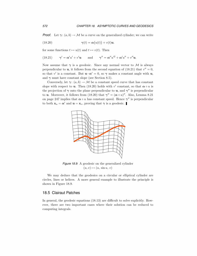
Figure 18.9: A geodesic on the generalized cylinder

(u, v) 7→ (u, sinu, v)

We may deduce that the geodesics on a circular or elliptical cylinder are

circles, lines or helices. A more general example to illustrate the principle is

shown in Figure 18.9.

18.5 Clairaut Patches

In general, the geodesic equations (18.13) are difficult to solve explicitly. How-

ever, there are two important cases where their solution can be reduced to

computing integrals.

18.5. CLAIRAUT PATCHES 573

Definition 18.23. Let M be a surface with metric

ds2 = Edu2 + 2F dudv +Gdv2.

(i) A uClairaut patch on M is a patch x : U → M for which

Ev = Gv = F = 0.

(ii) A vClairaut patch on M is a patch x : U → M for which

Eu = Gu = F = 0.

We work mainly with v-Clairaut patches, leaving the corresponding results for

u-Clairaut patches to the reader. To cite two examples, consider

(i) the standard parametrization of the unit sphere S2(1), having E = cos2 v,

F = 0 and G = 1.

(ii) the isothermal chart on S2(1) of Lemma 16.16 on page 519 (with v in place

of w), having E = G = sech v and F = 0.

Many others can be found from earlier chapters.

The Christoffel symbols for a v-Clairaut patch are considerably simpler than

those of a general patch. The following lemma is an immediate consequence of

Theorem 17.7 on page 539.

Lemma 18.24. For a v-Clairaut patch with ds2 = Edu2 +Gdv2 we have

Γ111 = 0, Γ2

11 =−Ev

2G,

Γ112 =

Ev

2E, Γ2

12 = 0,

Γ122 = 0, Γ2

22 =Gv

2G,

(18.22)

so that the geodesic equations (18.13) reduce to

u′′ +Ev

Eu′v′ = 0,

v′′ − Ev

2Gu′2 +

Gv

2Gv′2 = 0.

(18.23)

Some geodesics on a Clairaut patch are easy to determine.

Lemma 18.25. Let x : U → M be a v-Clairaut patch. Then:

(i) any v-parameter curve is a pregeodesic;


(ii) a u-parameter curve u 7→ x(u, v0) is a geodesic if and only if Ev(u, v0)

vanishes along u 7→ x(u, v0).

Proof. To prove (i), consider a v-parameter curve β defined by β(t) = x(u0, t).

It suffices by Lemma 18.18 to show that β′′(v)> is a scalar multiple of xv(u0, v).

Since xu and xv are orthogonal, this will be the case provided⟨β′′(v),xu(u0, v)

⟩

is zero. This equals

〈xvv(u0, v),xu(u0, v)〉 = 〈xv,xu〉′ − 〈xv,xuv〉

= Fv − 12Gu = 0,

the prime indicating differentiation with respect to t = v.

To prove (ii), we observe that if the u-parameter curve α(t) = x(t, v0) is a

geodesic, then

Ev(u, v0) = 2 〈xuv(u, v0),xu(u, v0)〉 = 2 〈xv,xu〉′ − 2 〈xv,xuu〉

= 2Fu − 2 〈xv,α′′〉 = 0,

where this time the prime denotes d/du. Conversely, if Ev(u, v0) = 0, then

〈xuu,xv〉 = 〈xu,xv〉u − 〈xu,xvu〉 = Fu − 12Ev = − 1

2Ev,

so that

〈α′′,xv〉 (u, v0) = − 12Ev(u, v0) = 0.

But also,

〈α′′,xu〉 = 12Eu = 0,

so that α is a geodesic.

We turn now to the problem of finding other geodesics on a Clairaut patch.

The key result we need is:

Theorem 18.26. (Clairaut’s relation) Let x : U → M be a v-Clairaut patch,

and let β be a geodesic whose trace is contained in x(U). Let θ be the angle

between β′ and xu. Then

√E ‖β′‖ cos θ is constant along β.(18.24)

Proof. We write β(t) = x(u(t), v(t)). From the assumption that Eu = 0 and

the first equation of (18.23), it follows that

(Eu′)′ = E′u′ + Eu′′ = Evv′u′ + Eu′′ = 0.

Hence there is a constant c such that

Eu′ = c.(18.25)

18.5. CLAIRAUT PATCHES 575

Furthermore,

‖β′‖ cos θ =〈xu,β

′〉‖xu‖

=〈xu,xuu

′ + xvv′〉

‖xu‖= ‖xu‖u′ =

√Eu′.

When this is combined with (18.25), we obtain (18.24).

Definition 18.27. The constant c given by (18.25) is called the slant of the

geodesic β in the v-Clairaut patch x. Then the angle between the geodesic and

xu is given by

cos θ =c

‖β′‖√E.

We next obtain information about geodesics on a Clairaut patch other than

those covered by Lemma 18.25.

Lemma 18.28. Let x : U → M be a v-Clairaut patch, and let β : (a, b) → R be

a unit-speed curve whose trace is contained in x(U). Write β(t) = x((u(t), v(t)).

If β is a geodesic, then there is a constant c such that

u′ =c

E,

v′ = ±√E − c2√EG

.

(18.26)

Conversely, if (18.26) holds, and if v′(t) 6= 0 for a < t < b, or if v′(t) = 0 for

a < t < b, then β is a geodesic.

Proof. Suppose that β is a unit-speed geodesic. The first equation of (18.26)

follows from (18.25). Furthermore,

1 =⟨β′,β′

⟩= 〈xuu

′ + xvv′, xuu

′ + xvv′〉

= Eu′2 +Gv′2 =c2

E+Gv′2,

so that

v′2 =1

G

(1 − c2

E

)=E − c2

EG.

Thus the second equation of (18.26) also holds.

Conversely, suppose that (18.26) holds. The first equation implies that

u′′ =( cE

)′

= −cEvv′

E2= −Evu

′v′

E.

Thus we see that the first equation of (18.23) is satisfied. Furthermore, β has

unit speed because

⟨β′,β′

⟩= Eu′2 +Gv′2 = E

( cE

)2

+G

(E − c2

EG

)= 1.


Next, when we differentiate the equation Gv′2 = 1 − Eu′2, we obtain

Gvv′3 + 2Gv′′v′ = −Evv

′u′2 − 2Eu′u′′(18.27)

= −Evv′u′2 + 2Eu′

(Ev

Eu′v′

)= Evv

′u′2.

Then (18.27) implies that the second equation of (18.23) is satisfied on any

interval where v′ is different from zero. On the other hand, on an interval

where v′ vanishes identically, the second equation of (18.26) implies that E is a

constant on that interval. Again, the second equation of (18.23) is satisfied.

Corollary 18.29. Let x : U → M be a v-Clairaut patch. A curve α : (a, b) → Mof the form

α(v) = x(u(v), v

)

is a pregeodesic if and only if there is a constant c such that

du

dv= ±c

√G

E(E − c2).(18.28)

Then c is the slant of α with respect to x.

Proof. There exists a unit-speed geodesic β reparametrizing α such that

β(s) = α(v(s)

)= x

(u(v(s)), v(s)

).

Then Lemma 18.28 implies that

du

ds=

c

Eand

dv

ds= ±

√E − c2√EG

.

Hence

du

dv=

du

ds

dv

ds

=

c

E

±√E − c2√EG

= ±c√

G

E(E − c2).

Conversely, if (18.28) holds, we define u′ and v′ by

u′

v′= ±c

√G

E(E − c2)and Eu′2 +Gv′2 = 1.

An easy calculation then shows that (18.26) holds, and so we get a pregeodesic.

18.6 Use of Clairaut Patches

Let us consider several examples of Clairaut patches and find their geodesics.

18.6. USE OF CLAIRAUT PATCHES 577

The Euclidean Plane in Polar Coordinates

The polar-coordinate parametrization of the xy-plane is

x(u, v) = (v cosu, v sinu, 0).(18.29)

It is clear that (18.29) is a v-Clairaut patch; indeed

E = v2, F = 0, G = 1.

Equation (18.28) becomes

du

dv= ± c√

v2(v2 − c2), or equivalently

cdv√v2(v2 − c2)

= ±du.

Carrying out the integration (done by computer in Notebook 18), we obtain

arctan

(c√

v2 − c2

)= ±(u− u0), or c = ±v sin(u− u0)

for some constant u0. This is merely the equation of a general straight line in

polar coordinates.

Solving the geodesic equations in polar coordinates is harder without the

techniques of the previous section. Finding the geodesics in the plane using

Cartesian coordinates is of course easier; see Exercise 13.

Surfaces of Revolution

The standard parametrization of a surface of revolution in R3 is

x(u, v) =(ϕ(v) cos u, ϕ(v) sinu, ψ(v)

).

Let us assume that ϕ(v) > 0; then ϕ(v) can be interpreted as the radius of the

parallel u 7→ (ϕ(v) cos u, ϕ(v) sin u, ψ(v)). Since

E = ϕ(v)2, F = 0 and G = ϕ′(v)2 + ψ′(v)2,

we see that Eu = Gu = F = 0; thus x is again a v-Clairaut patch, and the

equation for the geodesics is

du

dv= ±

√ϕ′2 + ψ′2

ϕ√ϕ2 − c2

.

Since the v-parameter curves are meridians, we recover Lemma 18.21 from

Lemma 18.25(i). Indeed, Theorem 18.26 is often quoted in the special case of a

surface of revolution. From Lemma 18.25, we deduce

Corollary 18.30. Let M be a surface of revolution in R3. Then a parallel is a

geodesic if an only if ϕ′(v0) = 0.


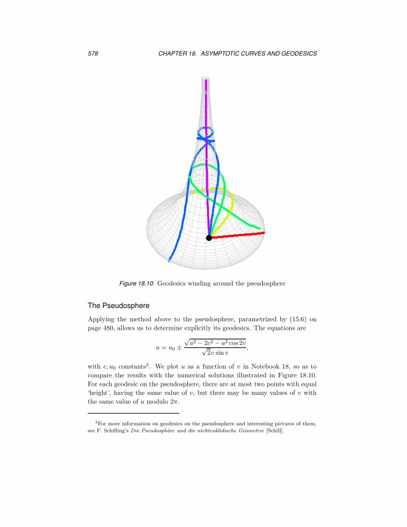
Figure 18.10: Geodesics winding around the pseudosphere

The Pseudosphere

Applying the method above to the pseudosphere, parametrized by (15.6) on

page 480, allows us to determine explicitly its geodesics. The equations are

u = u0 ±√a2 − 2c2 − a2 cos 2v√

2c sin v,

with c, u0 constants3. We plot u as a function of v in Notebook 18, so as to

compare the results with the numerical solutions illustrated in Figure 18.10.

For each geodesic on the pseudosphere, there are at most two points with equal

‘height’, having the same value of v, but there may be many values of v with

the same value of u modulo 2π.

3For more information on geodesics on the pseudosphere and interesting pictures of them,

see F. Schilling’s Die Pseudosphare und die nichteuklidische Geometrie [Schill].

18.7. EXERCISES 579

18.7 Exercises

1. Show that the differential equation for the asymptotic curves on a Monge

patch x(u, v) = (u, v, h(u, v)) is

huuu′2 + 2huvu

′v′ + hvvv′2 = 0.

2. Show that the differential equation for the asymptotic curves on a polar

patch of the form x(r, θ) = (r cos θ, r sin θ, h(r)) is

h′′(r)r′2 + h′(r)rθ′2 = 0.

M 3. Show that an asymptotic parametrization of a catenoid is given by

y(p, q) =(

cosp+ q

2cosh

−p+ q

2, sin

p+ q

2cosh

−p+ q

2,−p+ q

2

).

Plot this surface for 0 < p, q < 2π.

4. Find the differential equation for the asymptotic curves on the torus

x(u, v) =((a+ b cos v) cos u, (a+ b cos v) sin u, b sin v

).

M 5. Find the asymptotic curves of the generalized hyperbolic paraboloid

z = x2n − y2n.

Display some particular cases.

M 6. Find the asymptotic curves of the surface defined by

z = xmyn.

Display some particular cases.

7. Show that the Gaussian and mean curvatures of the (circular) helicoid

defined on page 376 are given by

K = − c2

(c2 + a2v2)2, H = 0.

Conclude that each u-parameter curve has constant torsion. Is this fact

known from an earlier chapter?

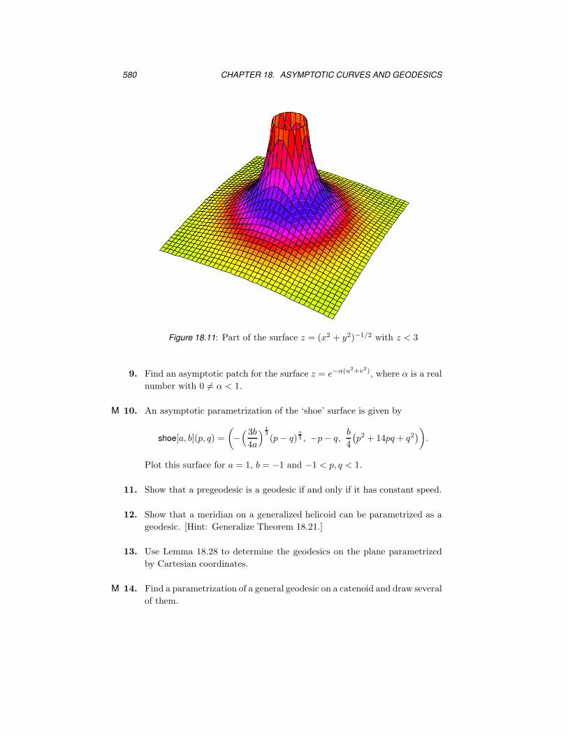
8. Find an asymptotic patch for the surface

z = (x2 + y2)α,

where α is a real number with 0 6= α < 1/2. Figure 18.11 is an ordinary

plot of the case α = −1/2 colored by Gaussian curvature.


Figure 18.11: Part of the surface z = (x2 + y2)−1/2 with z < 3

9. Find an asymptotic patch for the surface z = e−α(u2+v2), where α is a real

number with 0 6= α < 1.

M 10. An asymptotic parametrization of the ‘shoe’ surface is given by

shoe[a, b](p, q) =

(−

( 3b

4a

) 1

3

(p− q)2

3 , −p− q,b

4

(p2 + 14pq + q2

)).

Plot this surface for a = 1, b = −1 and −1 < p, q < 1.

11. Show that a pregeodesic is a geodesic if and only if it has constant speed.

12. Show that a meridian on a generalized helicoid can be parametrized as a

geodesic. [Hint: Generalize Theorem 18.21.]

13. Use Lemma 18.28 to determine the geodesics on the plane parametrized

by Cartesian coordinates.

M 14. Find a parametrization of a general geodesic on a catenoid and draw several

of them.

18.7. EXERCISES 581

15. Let β be a geodesic on a catenoid other than the center circle, and suppose

the initial velocity of β is perpendicular to the axis of revolution. Use

Clairaut’s relation (Theorem 18.26) to show that β approaches the center

curve asymptotically, but never reaches it.

M 16. Plot geodesics and geodesic circles on ellipsoids with two distinct axes and

on ellipsoids with three distinct axes.

17. Let α be an asymptotic curve defined by

α(t) = surfrev[α](u(t), v(t)

),

where surfrev[α] is the standard parametrization of a surface of revolution

given by (15.1). Show that u and v satisfy the differential equation

u′(t)2 =

(ϕ′′(t)ψ′(t) − ϕ′(t)ψ′′(t)

ϕ(t)ψ′(t)

)v′(t)2.

18. Fill in the proof of Lemma 18.24.

Documents

Asymptotic Curves and Geodesics on Surfaceswebmath2.unito.it/paginepersonali/sergio.console/Curve...Chapter 18 Asymptotic Curves and Geodesics on Surfaces In this chapter we begin