Shape and Curvature - unito.itwebmath2.unito.it/paginepersonali/sergio.console/CurveSuperfici/AG13.pdf · Chapter 13 Shape and Curvature In this chapter, we study the relationship

Chapter 13

Shape and Curvature

In this chapter, we study the relationship between the geometry of a regular

surface M in 3-dimensional space R3 and the geometry of R

3 itself. The basic

tool is the shape operator defined in Section 13.1. The shape operator at a point

p of M is a linear transformation S of the tangent space Mp that measures

how M bends in different directions. The shape operator can also be considered

to be (minus) the differential of the Gauss map of M (Proposition 13.5), and

its effect is illustrated using tangent vectors to coordinate curves on both the

original surface and the sphere (Figure 13.1).

In Section 13.2, we define a variant of the shape operator called normal

curvature. Given a tangent vector vp to a surface M, the normal curvature

k(vp) is a real number that measures how M bends in the direction vp. This

number is easy to understand geometrically because it is the curvature of the

plane curve formed by the intersection of M with the plane passing through vp

meeting M perpendicularly.

Techniques for computing the shape operator and normal curvature are given

in Section 13.3. The eigenvalues of the shape operator at p ∈ M are studied

at the end of that section. They turn out to be the maximum and minimum

of the normal curvature at p, the so-called principal curvatures, and the corre-

sponding eigenvectors are orthogonal. The principal curvatures are graphed for

the monkey saddle in Figure 13.6.

The most important curvature functions of a surface in R3 are the Gaussian

curvature and the mean curvature, both defined in Section 13.4. This leads to

a unified discussion of the the first, second and third fundamental forms. Two

separate techniques for computing curvature from the parametric representation

of a surface are described in Section 13.5, which includes calculations from

Notebook 13 with reference to Monge patches and other examples.

Section 13.6 is devoted to a global curvature theorem, while we discuss how

to compute the curvatures of nonparametric surfaces in Section 13.7.

385

386 CHAPTER 13. SHAPE AND CURVATURE

13.1 The Shape Operator

We want to measure how a regular surface M bends in R3. A good way to

do this is to estimate how the surface normal U changes from point to point.

We use a linear operator called the shape operator to calculate the bending of

M. The shape operator came into wide use after its introduction in O’Neill’s

book [ON1]; however, it occurs much earlier, for example, implicitly in Blashke’s

classical book [Blas2]1, and explicitly in [BuBu]2.

The shape operator applied to a tangent vector vp is the negative of the

derivative of U in the direction vp:

Definition 13.1. Let M ⊂ R3 be a regular surface, and let U be a surface

normal to M defined in a neighborhood of a point p ∈ M. For a tangent vector

vp to M at p we put

S(vp) = −DvU.

Then S is called the shape operator.

Derivatives of vector fields were discussed in Section 9.5, and regular surfaces

in Section 10.3. The precise definition of DvU relies on Lemma 9.40, page 281,

since U is not defined away from the surface M.

It is easy to see that the shape operator of a plane is identically zero at

all points of the plane. For a nonplanar surface the surface normal U will

twist and turn from point to point, and S will be nonzero. At any point of an

orientable regular surface there are two choices for the unit normal: U and −U.

The shape operator corresponding to −U is the negative of the shape operator

corresponding to U. If M is nonorientable, we have seen that a surface normal

U cannot be defined continuously on all of M. This does not matter in the

present chapter, because all calculations involving U are local, so it suffices to

perform the local calculations on an open subset U of M where U is defined

continuously.

1

Wilhelm Johann Eugen Blaschke (1885–1962). Austrian-German mathe-

matician. In 1919 he was appointed to a chair in Hamburg, where he built

an important school of differential geometry.

2Around 1900 the Gibbs–Heaviside vector analysis notation (which one can read about in

the interesting book [Crowe]) spread to differential geometry, although its use was controversial

for another 30 years. Blashke’s [Blas2] was one of the first differential geometry books to use

vector analysis. The book coauthored by Burali-Forti and Burgatti [BuBu] contains an amus-

ing attack on those resisting the new vector notation. In the multivolume works of Darboux

[Darb1] and Bianchi [Bian] most formulas are written component by component. Compact

vector notation, of course, is indispensable nowadays both for humans and for computers.

13.1. SHAPE OPERATOR 387

Recall (Lemma 10.26, page 299) that any point q in the domain of definition

of a regular patch x : U → R3 has a neighborhood Uq of q such that x(Uq) is a

regular surface. Therefore, the shape operator of a regular patch is also defined.

Conversely, we can use patches on a regular surface M ⊂ R3 to calculate the

shape operator of M.

The next lemmas establish some elementary properties.

Lemma 13.2. Let x : U → R3 be a regular patch. Then

S(xu) = −Uu and S(xv) = −Uv.

Proof. Fix v and define a curve α by α(u) = x(u, v). Then by Lemma 9.40,

page 281, we have

S(

xu(u, v))

= S(

α′(u))

= −Dα′(u)U = −(U ◦ α)′(u).

But (U ◦ α)′ is just Uu. Similarly, S(xv) = −Uv.

Lemma 13.3. At each point p of a regular surface M ⊂ R3, the shape operator

is a linear map

S : Mp −→ Mp.

Proof. That S is linear follows from the fact that Dav+bw = aDv + bDw. To

prove that S maps Mp into Mp (instead of merely into R3p), we differentiate

the equation U · U = 1 and use (9.12) on page 276:

0 = vp[U · U] = 2(DvU) · U(p) = −2S(vp) · U(p),

for any tangent vector vp. Since S(vp) is perpendicular to U(p), it must be

tangent to M; that is, S(vp) ∈ Mp.

Next, we find an important relation between the shape operator of a surface

and the acceleration of a curve on the surface.

Lemma 13.4. If α is a curve on a regular surface M ⊂ R3, then

α′′· U = S(α′) · α′.

Proof. We restrict the vector field U to the curve α and use Lemma 9.40.

Since α(t) ∈ M for all t, the velocity α′ is always tangent to M, so

α′· U = 0.

When we differentiate this equation and use Lemmas 13.2 and 13.3, we obtain

α′′· U = −U′

· α′ = S(α′) · α′.

Observe that α′′· U can be interpreted geometrically as the component of the

acceleration of α that is perpendicular to M.


Figure 13.1: Coordinate curves and tangent vectors, together with

(on the right) their Gauss images

Lemma 13.2 allows us to illustrate −S by its effect on tangent vectors to

coordinate curves to M. These are mapped to the tangent vectors to the cor-

responding curves on the unit sphere defined by U. This is expressed more

invariantly by the next result that asserts that −S is none other than the tan-

gent map of the Gauss map.

Proposition 13.5. Let M be a regular surface in R3 oriented by a unit normal

vector field U. View U as the Gauss map U : M → S2(1), where S2(1) denotes

the unit sphere in R3. If vp is a tangent vector to M at p ∈ M, then U∗(vp)

is parallel to −S(vp) ∈ Mp.

Proof. By Lemma 9.10, page 269, we have

U∗(vp) =(

vp[u1], vp[u2], vp[u3])

U(p).

On the other hand, Lemma 9.28, page 275, implies that

−S(vp) = DvU =(

vp[u1], vp[u2], vp[u3])

p.

Since the vectors (vp[u1],vp[u2],vp[u3])U(p) and (vp[u1],vp[u2],vp[u3])p are

parallel, the lemma follows.

We conclude this introductory section by noting a fundamental relationship

between shape operators of surfaces and Euclidean motions of R3.

Theorem 13.6. Let F : R3 → R

3 be an orientation-preserving Euclidean mo-

tion, and let M1 and M2 be oriented regular surfaces such that F (M1) = M2.

Then

13.2. NORMAL CURVATURE 389

(i) the unit normals U1 and U2 of M1 and M2 can be chosen so that

F∗(U1) = U2;

(ii) the shape operators S1 and S2 of the two surfaces (with the choice of unit

normals given by (i)) are related by S2 ◦ F∗ = F∗ ◦ S1.

Proof. Since F∗ preserves lengths and inner products, it follows that F∗(U1)

is perpendicular to M2 and has unit length. Hence F∗(U1) = ±U2; we choose

the plus sign at all points of M2. Let p ∈ M1 and vp ∈ M1p, and let wF (p) =

F∗(vp). A Euclidean motion is an affine transformation, so by Lemma 9.35,

page 278, we have

(S2 ◦ F∗)(vp) = S2(wF (p)) = −DwU2 = −DwF∗(U1)

= −F∗(DvU1) = (F∗ ◦ S1)(vp).

Because vp is arbitrary, we have S2 ◦ F∗ = F∗ ◦ S1.

13.2 Normal Curvature

Although the shape operator does the job of measuring the bending of a surface

in different directions, frequently it is useful to have a real-valued function, called

the normal curvature, which does the same thing. We shall define it in terms of

the shape operator, though it is worth bearing in mind that normal curvature

is explicitly a much older concept (see [Euler3], [Meu] and Corollary 13.20).

First, we need to make precise the notion of direction on a surface.

Definition 13.7. A direction ` on a regular surface M is a 1-dimensional sub-

space of (that is, a line through the origin in) a tangent space to M.

A nonzero vector vp in a tangent space Mp determines a unique 1-dimensional

subspace `, so we can use the terminology ‘the direction vp’ to mean `, provided

the sign of vp is irrelevant.

Definition 13.8. Let up be a tangent vector to a regular surface M ⊂ R3 with

‖up‖ = 1. Then the normal curvature of M in the direction up is

k(up) = S(up) · up.

More generally, if vp is any nonzero tangent vector to M at p, we put

k(vp) =S(vp) · vp

‖vp‖2.(13.1)


If ` is a direction in a tangent space Mp to a regular surface M ⊂ R3, then

k(vp) is easily seen to be the same for all nonzero tangent vectors vp in ` (this

is Exercise 9). Therefore, we call the common value of the normal curvature the

normal curvature of the direction `.

Let us single out two kinds of directions.

Definition 13.9. Let ` be a direction in a tangent space Mp, where M ⊂ R3

is a regular surface. If the normal curvature of ` is zero, we say that ` is an

asymptotic direction. Similarly, if the normal curvature vanishes on a tangent

vector vp to M, we say that vp is an asymptotic vector. An asymptotic curve on

M is a curve whose trace lies on M and whose tangent vector is everywhere

asymptotic.

Asymptotic curves will be studied in detail in Chapter 18.

Definition 13.10. Let M be a regular surface in R3 and let p ∈ M. The

maximum and minimum values of the normal curvature k of M at p are called

the principal curvatures of M at p and are denoted by k1 and k2. Unit vectors

e1, e2 ∈ Mp at which these extreme values occur are called principal vectors.

The corresponding directions are called principal directions. A principal curve on

M is a curve whose trace lies on M and whose tangent vector is everywhere

principal.

The principal curvatures measure the maximum and minimum bending of a

regular surface M at each point p ∈ M. Principal curves will be studied again

in Section 15.2, and in more detail in Chapter 19.

There is an important interpretation of normal curvature of a regular surface

as the curvature of a space curve.

Lemma 13.11. (Meusnier) Let up be a unit tangent vector to M at p, and let

β be a unit-speed curve in M with β(0) = p and β′(0) = up. Then

k(up) = κ[β](0) cos θ,(13.2)

where κ[β](0) is the curvature of β at 0, and θ is the angle between the normal

N(0) of β and the surface normal U(p). Thus all curves lying on a surface Mand having the same tangent line at a given point p ∈ M have the same normal

curvature at p.

Proof. Suppose that κ[β](0) 6= 0. By Lemma 13.4 and Theorem 7.10, page 197,

we have

k(up) = S(up) · up = β′′(0) · U(p)(13.3)

= κ[β](0)N(0) · U(p) = κ[β](0) cos θ.

In the exceptional case that κ[β](0) = 0, the normal N(0) is not defined, but

we still have k(up) = 0.

13.2. NORMAL CURVATURE 391

To understand the meaning of normal curvature geometrically, we need to

find curves on a surface to which we can apply Lemma 13.11.

Definition 13.12. Let M ⊂ R3 be a regular surface and up a unit tangent vec-

tor to M. Denote by Π(

up,U(p))

the plane determined by up and the surface

normal U(p). The normal section of M in the up direction is the intersection

of Π(

up,U(p))

and M.

Corollary 13.13. Let β be a unit-speed curve which lies in the intersection of

a regular surface M ⊂ R3 and one of its normal sections Π through p ∈ M.

Assume that β(0) = p and put up = β′(0). Then the normal curvature k(up)

of M and the curvature of β are related by

k(up) = ±κ[β](0).(13.4)

Proof. We may assume that κ[β](0) 6= 0, for otherwise (13.4) is an obvious

consequence of (13.2). Since β has unit speed, κ[β](0)N(0) = β′′(0) is per-

pendicular to β′(0). On the other hand, both U(p) and N(0) lie in Π , so

the only possibility is N(0) = ±U(p). Hence cos θ = ±1 in (13.2), and so we

obtain (13.4).

Figure 13.2: Normal sections to a paraboloid through asymptotic curves

Corollary 13.13 gives an excellent method for estimating normal curvature

visually. For a regular surface M ⊂ R3, suppose we want to know the normal

curvature in various directions at p ∈ M. Each unit vector up ∈ Mp, together

with the surface normal U(p), determines a plane Π(

up,U(p))

. Then the

normal section in the direction up is the intersection of Π(

up,U(p))

and M.

This is a plane curve in Π(

up,U(p))

whose curvature is given by (13.4). There

are three cases:


• If k(up) > 0, then the normal section is bending in the same direction as

U(p). Hence in the up direction M is bending toward U(p).

• If k(up) < 0, then the normal section is bending in the opposite direction

from U(p). Hence in the up direction M is bending away from U(p).

• If k(up) = 0, then the curvature of the normal section vanishes at p so

the normal to a curve in the normal section is undefined. It is impossible

to conclude that there is no bending of M in the up direction since κ[β]

might vanish only at p. But in some sense the bending is small.

As the unit tangent vector up turns, the surface may bend in different ways.

A good example of this occurs at the center point of a hyperbolic paraboloid.

Figure 13.3: Normal sections to a paraboloid through principal curves

In Figure 13.2, both normal sections intersect the hyperbolic paraboloid in

straight lines, and the normal curvature determined by each of these sections

vanishes. These straight lines are in fact asymptotic curves, whereas the sec-

tions shown in Figure 13.3 intersect the surface in curves tangent to principal

directions (recall Definitions 13.9 and 13.10). In the second case, the normal

curvature determined by one section is positive, and that determined by the

other is negative.

The normal sections at the center of a monkey saddle are similar to those of

the hyperbolic paraboloid, but more complicated. In this case, there are three

asymptotic directions passing through the center point o of the monkey saddle.

It is this fact that forces S to vanish as a linear transformation of the tangent

space ToM at the point o itself.

13.3. CALCULATION OF THE SHAPE OPERATOR 393

Figure 13.4: Normal sections to a monkey saddle

13.3 Calculation of the Shape Operator

Symmetric linear transformations are much easier to work with than general

linear transformations. We shall exploit this in developing the theory of the

shape operator, which fortunately falls into this category.

Lemma 13.14. The shape operator of a regular surface M is symmetric or

selfadjoint, meaning that

S(vp) · wp = vp · S(wp)

for all tangent vectors vp,wp to M.

Proof. Let x be an injective regular patch on M. We differentiate the formula

U · xu = 0 with respect to v and obtain

0 =∂

∂v(U · xu) = Uv · xu + U · xuv,(13.5)

where Uv is the derivative of the vector field v 7→ U(u, v) along any v-parameter

curve. Since Uv = −S(xv), equation (13.5) becomes

S(xv) · xu = U · xuv.(13.6)

Similarly,

S(xu) · xv = U · xvu.(13.7)


From (13.6), (13.7) and the fact that xuv = xvu we get

S(xu) · xv = U · xvu = U · xuv = S(xv) · xu.(13.8)

The proof is completed by expressing vp,wp in terms of xu,xv and using

linearity.

Definition 13.15. Let x : U → R3 be a regular patch. Then

e = −Uu · xu = U · xuu,

f = −Uv · xu = U · xuv = U · xvu = −Uu · xv,

g = −Uv · xv = U · xvv.

(13.9)

Classically, e, f, g are called the coefficients of the second fundamental form of x.

In Section 12.1 we wrote the metric as

ds2 = Edu2 + 2F dudv +Gdv2,

and E,F,G are called the coefficients of the first fundamental form of x. The

quantity

edu2 + 2f dudv + gdv2

has a more indirect interpretation, given on page 402. The notation e, f, g is

that used in most classical differential geometry books, though many authors

use L,M,N in their place. Incidentally, Gauss used the notation D, D′, D′′ for

the respective quantities e√EG− F 2, f

√EG− F 2, g

√EG− F 2.

Theorem 13.16. (The Weingarten3 equations) Let x : U → R3 be a regular

patch. Then the shape operator S of x is given in terms of the basis {xu,xv} by

−S(xu) = Uu =f F − eG

EG− F 2xu +

eF − f E

EG− F 2xv,

−S(xv) = Uv =gF − f G

EG− F 2xu +

f F − gE

EG− F 2xv.

(13.10)

Proof. Since x is regular, and xu and xv are linearly independent, we can write

−S(xu) = Uu = a11xu + a21xv,

−S(xv) = Uv = a12xu + a22xv,(13.11)

3

Julius Weingarten (1836–1910). Professor at the Technische Universitat in

Berlin. A surface for which there is a definite functional relation between

the principal curvatures is called a Weingarten surface.

13.3. CALCULATION OF THE SHAPE OPERATOR 395

for some functions a11, a21, a12, a22, which we need to compute. We take the

scalar product of each of the equations in (13.11) with xu and xv, and obtain

−e = Ea11 + Fa21,

−f = Fa11 +Ga21,

−f = Ea12 + Fa22,

−g = Fa12 +Ga22.

(13.12)

Equations (13.12) can be written more concisely in terms of matrices:

−(

e f

f g

)

=

(

E F

F G

)(

a11 a12

a21 a22

)

;

hence(

a11 a12

a21 a22

)

= −(

E F

F G

)

−1(

e f

f g

)

=−1

EG− F 2

(

G −F−F E

)(

e f

f g

)

=−1

EG− F 2

(

Ge− Ff Gf − Fg

−Fe+ Ef −Ff + Eg

)

.

The result follows from (13.11).

Although S is a symmetric linear operator, its matrix (aij) relative to {xu,xv}need not be symmetric, because xu and xv are not in general perpendicular to

one another.

There is also a way to express the normal curvature in terms of E,F,G and

e, f, g:

Lemma 13.17. Let M ⊂ R3 be a regular surface and let p ∈ M. Let x be an

injective regular patch on M with p = x(u0, v0). Let vp ∈ Mp and write

vp = a xu(u0, v0) + b xv(u0, v0).

Then the normal curvature of M in the direction vp is

k(vp) =ea2 + 2f ab+ g b2

Ea2 + 2F ab+Gb2.

Proof. We have ‖vp‖2 = ‖axu + bxv‖2 = a2E + 2abF + b2G, and

S(vp) · vp =(

aS(xu) + bS(xv))

· (axu + bxv) = a2e+ 2abf + b2g.

The result follows from (13.1).


Eigenvalues of the Shape Operator

We first recall an elementary version of the spectral theorem in linear algebra.

Lemma 13.18. Let V be a real n-dimensional vector space with an inner prod-

uct and let A : V → V be a linear transformation that is self-adjoint with respect

to the inner product. Then the eigenvalues of A are real and A is diagonalizable:

there is an orthonormal basis {e1, . . . , en} of V such that

Aej = λjej for > j = 1, . . . , n.

Lemma 13.14 tells us that the shape operator S is a self-adjoint linear op-

erator on each tangent space to a regular surface in R3, so the eigenvalues of S

must be real. These eigenvalues are important geometric quantities associated

with each regular surface in R3. Instead of proving Lemma 13.18 in its full

generality, we prove it for the special case of the shape operator.

Lemma 13.19. The eigenvalues of the shape operator S of a regular surface

M ⊂ R3 at p ∈ M are precisely the principal curvatures k1 and k2 of M at p.

The corresponding unit eigenvectors are unit principal vectors, and vice versa.

If k1 = k2, then S is scalar multiplication by their common value. Otherwise,

the eigenvectors e1, e2 of S are perpendicular, and S is given by

Se1 = k1e1, Se2 = k2e2.(13.13)

Proof. Consider the normal curvature as a function k : S1p → R, where S1

p

is the set of unit tangent vectors in the tangent space Mp. Since S1p is a

circle, it is compact, and so k achieves its maximum at some unit vector, call it

e1 ∈ S1p. Choose e2 to be any vector in S1

p perpendicular to e1, so {e1, e2} is

an orthonormal basis of Mp and

Se1 = (Se1 · e1)e1 + (Se1 · e2)e2,

Se2 = (Se2 · e1)e1 + (Se2 · e2)e2.(13.14)

Define a function u = u(θ) by setting u(θ) = e1 cos θ + e2 sin θ, and write

k(θ) = k(

u(θ))

. Then

k(θ) = (Se1 · e1) cos2θ + 2(Se1 · e2) sin θ cos θ + (Se2 · e2) sin2θ,(13.15)

so that

d

dθk(θ) = 2(Se2 · e2 − Se1 · e1) sin θ cos θ + 2(Se1 · e2)(cos2θ − sin2θ).

In particular,

0 =dk

dθ(0) = 2Se1 · e2,(13.16)

13.4. GAUSSIAN AND MEAN CURVATURE 397

because k(θ) has a maximum at θ = 0. Then (13.14) and (13.16) imply (13.13).

From (13.13) it follows that both e1 and e2 are eigenvectors of S, and from

(13.15) it follows that the principal curvatures of M at p are the eigenvalues of

S. Hence the lemma follows.

The principal curvatures determine the normal curvature completely:

Corollary 13.20. (Euler) Let k1(p), k2(p) be the principal curvatures of a reg-

ular surface M ⊂ R3 at p ∈ M, and let e1, e2 be the corresponding unit

principal vectors. Let θ denote the oriented angle from e1 to up, so that

up = e1 cos θ + e2 sin θ. Then the normal curvature k(up) is given by

k(up) = k1(p) cos2θ + k2(p) sin2θ.(13.17)

Proof. Since S(e1) · e2 = 0, (13.15) reduces to (13.17).

13.4 Gaussian and Mean Curvature

The notion of the curvature of a surface is a great deal more complicated than

the notion of curvature of a curve. Let α be a curve in R3, and let p be a

point on the trace of α. The curvature of α at p measures the rate at which

α leaves the tangent line to α at p. By analogy, the curvature of a surface

M ⊂ R3 at p ∈ M should measure the rate at which M leaves the tangent

plane to M at p. But a difficulty arises for surfaces that was not present for

curves: although a curve can separate from one of its tangent lines in only two

directions, a surface separates from one of its tangent planes in infinitely many

directions. In general, the rate of departure of a surface from one of its tangent

planes depends on the direction.

There are several competing notions for the curvature of a surface in R3:

• the normal curvature k;

• the principal curvatures k1, k2;

• the mean curvature H ;

• the Gaussian curvature K.

We defined normal curvature and the principal curvatures of a surface M ⊂ R3

in Section 13.2. In the present section, we give the definitions of the Gaussian

and mean curvatures; these are the most important functions in surface theory.

First, we recall some useful facts from linear algebra. If S : V → V is a linear

transformation on a vector space V , we may define the determinant and trace

of S, written detS and trS, merely as the determinant and trace of the matrix


A representing S with respect to any chosen basis. If P is an invertible matrix

representing a change in basis then S is represented by P−1AP with respect to

the new basis, but standard properties of the determinant and trace functions

ensure thatdet(P−1AP ) = detA,

tr(P−1AP ) = trA,(13.18)

so that our definitions are independent of the choice of basis.

Definition 13.21. Let M be a regular surface in R3. The Gaussian curvature

K and mean curvature H of M are the functions K,H : M → R defined by

K(p) = det(

S(p))

and H(p) = 12 tr(

S(p))

.(13.19)

Note that although the shape operator S and the mean curvature H depend on

the choice of unit normal U, the Gaussian curvature K is independent of that

choice. The name ‘mean curvature’ is due to Germain4.

Definition 13.22. A minimal surface in R3 is a regular surface for which the

mean curvature vanishes identically. A regular surface is flat if and only if its

Gaussian curvature vanishes identically.

We shall see in Chapter 16 that surfaces of minimal area are indeed minimal in

the sense of Definition 13.22.

The Gaussian curvature permits us to distinguish four kinds of points on a

surface.

Definition 13.23. Let p be a point on a regular surface M ⊂ R3. We say that

• p is elliptic if K(p) > 0 (equivalently, k1 and k2 have the same sign);

• p is hyperbolic if K(p) < 0 (equivalently, k1 and k2 have opposite signs);

• p is parabolic if K(p) = 0, but S(p) 6= 0 (equivalently, exactly one of k1

and k2 is zero);

• p is planar if K(p) = 0 and S(p) = 0 (equivalently, k1 = k2 = 0).

It is usually possible to glance at almost any surface and recognize which

points are elliptic, hyperbolic, parabolic or planar. Consider, for example, the

paraboloids shown in Figure 12.10 on page 375. Not surprisingly, all the points

4

Sophie Germain (1776–1831). French mathematician, best known for

her work on elasticity and Fermat’s last theorem. Germain (under the

pseudonym ‘M. Blanc’) corresponded with Gauss regarding her results in

geometry and number theory.


on the left-hand elliptical paraboloid are elliptic, and all those on the right-

hand hyperbolic paraboloid are hyperbolic. Calculations from the next section

show that the monkey surface (13.25) has all its points hyperbolic except for

its central point, o = (0, 0, 0), which is planar. This corresponds to the fact,

illustrated in Figure 13.5, that its Gaussian curvature K both vanishes and

achieves an absolute maximum at o.

-2

-1

0

1

2

-3

-2

-1

0-2

-1

0

1

2

Figure 13.5: Gaussian curvature of the monkey saddle

There are two especially useful ways of choosing a basis of a tangent space

to a surface in R3. Each gives rise to important formulas for the Gaussian and

mean curvatures, which are presented in turn by the following proposition and

subsequent theorem.

Proposition 13.24. The Gaussian curvature and mean curvature of a regular

surface M ⊂ R3 are related to the principal curvatures by

K = k1k2 and H = 12 (k1 + k2).

Proof. If we choose an orthonormal basis of eigenvectors of S for Mp, the

matrix of S with respect to this basis is diagonal so that

K = det

(

k1 0

0 k2

)

= k1k2

H = 12 tr

(

k1 0

0 k2

)

= 12 (k1 + k2).


Let M ⊂ R3 be a regular surface. The Gaussian and mean curvatures are

functions K,H : M → R; we have written K(p) and H(p) for their values at

p ∈ M. We need a slightly different notation for a regular patch x : U → R3.

Strictly speaking, K and H are functions defined on x(U) → R. However, we

follow conventional notation and abbreviate K ◦ x to K and H ◦ x to H . Thus

K(u, v) and H(u, v) will denote the values of the Gaussian and mean curvatures

at x(u, v).

Theorem 13.25. Let x : U → R3 be a regular patch. The Gaussian curvature

and mean curvature of x are given by the formulas

K =eg − f2

EG− F 2,(13.20)

H =eG− 2fF + gE

2(EG− F 2),(13.21)

where e, f, g are the coefficients of the second fundamental form relative to x,

and E,F,G are the coefficients of the first fundamental form.

Proof. This time we computeK andH using the basis {xu,xv}, and the matrix

−1

EG− F 2

(

Ge− Ff Gf − Fg

−Fe+ Ef −Ff + Eg

)

of Theorem 13.16. Taking the determinant and half the trace yields

K =(fF − eG)(fF − gE) − (eF − fE)(gF − fG)

(EG− F 2)2=

eg − f2

EG− F 2,

and

H = − (fF − eG) + (fF − gE)

2(EG− F 2)=eG− 2fF + gE

2(EG− F 2).

The importance of Proposition 13.24 is theoretical, that of Theorem 13.25

more practical. Usually, one uses Theorem 13.25 to compute K and H , and

afterwards Proposition 13.24 to find the principal curvatures. More explicitly,

Corollary 13.26. The principal curvatures k1, k2 are the roots of the quadratic

equation

x2 − 2Hx+K = 0.

Thus we can choose k1, k2 so that

k1 = H +√

H2 −K and k2 = H −√

H2 −K.(13.22)


Corollary 13.27. Suppose that M ⊂ R3 has negative Gaussian curvature K

at p. Then:

(i) there are exactly two asymptotic directions at p, and they are bisected by

the principal directions;

(ii) the two asymptotic directions at p are perpendicular if and only if the

mean curvature H of M vanishes at p.

Proof. Let e1 and e2 be unit principal vectors corresponding to k1(p) and

k2(p). ThenK(p) = k1(p)k2(p) < 0 implies that k1(p) and k2(p) have opposite

signs. Thus, there exists θ with 0 < θ < π/2 such that

tan2θ = −k1(p)

k2(p).

Put up(θ) = e1 cos θ + e2 sin θ. Then (13.17) implies that up(θ) and up(−θ)are linearly independent asymptotic vectors at p. The angle between up(θ) and

up(−θ) is 2θ, and it is clear that e1 bisects the angle between up(θ) and up(−θ).This proves (i). For (ii) we observe that H(p) = 0 if and only if θ equals ±π/4,

up to integral multiples of π.

The Three Fundamental Forms

In classical differential geometry, there are frequent references to the ‘second

fundamental form’ of a surface in R3, a notion that is essentially equivalent to

the shape operator S. Such references can for example be found in the influential

textbook [Eisen1] of Eisenhart5.

Definition 13.28. Let M be a regular surface in R3. The second fundamental

form is the symmetric bilinear form II on a tangent space Mp given by

II(vp,wp) = S(vp) · wp

for vp,wp ∈ Mp.

Since there is a second fundamental form, there must be a first fundamental

form. It is nothing but the inner product between tangent vectors:

I(vp,wp) = vp · wp.

5Luther Pfahler Eisenhart (1876–1965). American differential geometer and

dean at Princeton University.


Note that the first fundamental form I can in a sense defined whether or not

the surface is in R3; this is the basis of theory to be discussed in Chapter 26.

The following lemma is an immediate consequence of the definitions.


I(axu + bxv, axu + bxv) = Ea2 + 2F ab+Gb2,

II(axu + bxv, axu + bxv) = ea2 + 2f ab+ g b2.

The normal curvature is therefore given by

k(vp) =II(vp,vp)

I(vp,vp)

for any nonzero tangent vector vp.

This lemma explains why we call E,F,G the coefficients of the first fundamental

form, and e, f, g the coefficients of the second fundamental form.

Finally, there is also a third fundamental form III for a surface in R3 given by

III(vp,wp) = S(vp) · S(wp)

for vp,wp ∈ Mp. Note that III, in contrast to II, does not depend on the

choice of surface normal U. The third fundamental form III contains no new

information, since it is expressible in terms of I and II.

Lemma 13.30. Let M ⊂ R3 be a regular surface. Then the following relation

holds between the first, second and third fundamental forms of M:

III − 2H II +K I = 0,(13.23)

where H and K denote the mean curvature and Gaussian curvature of M.

Proof. Although (13.23) follows from Corollary 13.26 and the Cayley–Hamilton6

Theorem (which states that a matrix satisfies its own characteristic polynomial),

we prefer to give a direct proof.

First, note that the product H II is independent of the choice of surface

normal U. Hence (13.23) makes sense whether or not M is orientable. To

6

Sir William Rowan Hamilton (1805–1865). Irish mathematician, best

known for having been struck with the concept of quaternions as he crossed

Brougham Bridge in Dublin (see Chapter 23), and for his work in dynam-

ics.

13.5. MORE CURVATURE CALCULATIONS 403

prove it, we observe that since its left-hand side is a symmetric bilinear form, it

suffices to show that for each p ∈ M and some basis {e1, e2} of Mp we have

(III − 2H II +K I)(ei, ej) = 0,(13.24)

for i, j = 1, 2. We choose e1 and e2 to be linearly independent principal vectors

at p. Then

(III − 2H II +K I)(e1, e2) = 0

because each term vanishes separately. Furthermore,

(III− 2H II +K I)(ei, ei) = k2i − (k1 + k2)ki + k1k2 = 0

for i = 1 and 2, as required.

13.5 More Curvature Calculations

In this section, we show how to compute by hand the Gaussian curvature K

and the mean curvature H for a monkey saddle and a torus. Along the way we

compute the coefficients of their first and second fundamental forms.

The Monkey Saddle

For the surface parametrized by

x(u, v) = monkeysaddle(u, v) = (u, v, u3 − 3uv2),(13.25)

and described on page 304, we easily compute

xu(u, v) = (1, 0, 3u2 − 3v2), xv(u, v) = (0, 1,−6uv),

xuu(u, v) = (0, 0, 6u), xuv(u, v) = (0, 0,−6v), xvv(u, v) = (0, 0,−6u).

Therefore,

E = 1 + 9(u2 − v2)2, F = −18uv(u2 − v2), G = 1 + 36u2v2,

and by inspection a unit surface normal is

U =(−3u2 + 3v2, 6uv, 1)

√

1 + 9u4 + 18u2v2 + 9v4,

so that

e = U · xuu =6u

√

1 + 9u4 + 18u2v2 + 9v4,

f = U · xuv =−6v

√

1 + 9u4 + 18u2v2 + 9v4,

g = U · xvv =−6u

√

1 + 9u4 + 18u2v2 + 9v4.


Theorem 13.25 yields

K =−36(u2 + v2)

(1 + 9u4 + 18u2v2 + 9v4)2, H =

−27u5 + 54u3v2 + 81uv4

(1 + 9u4 + 18u2v2 + 9v4)3/2.

A glance at these expressions shows that o = (0, 0, 0) is a planar point of the

monkey saddle and that every other point is hyperbolic. Furthermore, the

Gaussian curvature of the monkey saddle is invariant under all rotations about

the z-axis, even though the monkey saddle itself does not have this property.

The principal curvatures are determined by Corollary 13.26, and are easy to

plot. Figure 13.6 shows graphically their singular nature at the point o, which

contrasts with the surface itself sandwiched in the middle.

Figure 13.6: Principal curvatures of the monkey saddle

Alternative Formulas

Classically, the standard formulas for computing K and H for a patch x are

(13.20) and (13.21). It is usually too tedious to compute K and H by hand

in one step. Therefore, the functions E,F,G and e, f, g need to be computed

before any of the curvature functions are calculated. The computation of E,

F , G is straightforward: first one computes the first derivatives xu and xv and

then the dot products E = xu · xu, F = xu · xv and G = xv · xv.

There are two methods for computing e, f, g. The direct approach using the

definitions necessitates computing the surface normal via equation (10.11) on

page 295, and then using the definition (13.9). The other method, explained in


the next lemma, avoids computation of the surface normal; it uses instead the

vector triple product which can be computed as a determinant.


e =[xuu xu xv]√EG− F 2

, f =[xuv xu xv]√EG− F 2

, g =[xvv xu xv]√EG− F 2

.

Proof. From (7.4) and (13.9) it follows that

e = xuu · U = xuu ·

xu × xv

‖xu × xv‖=

[xuu xu xv]√EG− F 2

.

The other formulas are proved similarly.

On the other hand, at least theoretically, we can compute K and H for a

regular patch x directly in terms of the first and second derivatives of x. Here

are the relevant formulas.

Corollary 13.32. Let x : U → R3 be a regular patch. The Gaussian and mean

curvatures of M are given by the formulas

K =[xuu xu xv][xvv xu xv] − [xuv xu xv]2

(

‖xu‖2‖xv‖2 − (xu · xv)2)2 ,(13.26)

H =[xuu xu xv]‖xv‖2 − 2[xuv xu xv](xu · xv) + [xvv xu xv]‖xu‖2

2(

‖xu‖2‖xv‖2 − (xu · xv)2)3/2

.(13.27)

Proof. The equations follow from (13.20), (13.21) and Lemma 13.31 when we

write out e, f, g and E,F,G explicitly in terms of dot products.

Equations 13.26 and 13.27 are used effectively in Notebook 13. They are usually

too complicated for hand calculation, but we do use them below in the case of

the torus.

It is neither enlightening nor useful to write out the formulas for the principal

curvatures in terms of E,F,G, e, f, g in general. However, there is one special

case when such formulas for k1, k2 are worth noting.

Corollary 13.33. Let x : U → R3 be a regular patch for which f = F = 0. With

respect to this patch, the principal curvatures are e/E and g/G.

Proof. When F = f = 0, the Weingarten equations (13.10) reduce to

S(xu) =e

Exu and S(xv) =

g

Gxv.

By definition, e/E and g/G are the eigenvalues of the shape operator S.


The Sphere

We compute the principal curvatures of the patch

x(u, v) = sphere[a](u, v) =(

a cos v cosu, a cos v sinu, a sin v)

(13.28)

of the sphere with center o = (0, 0, 0) and radius a. We find that

xu(u, v) =(

− a cos v sinu, a cos v cosu, 0)

,

xv(u, v) =(

− a sin v cosu, −a sin v sinu, a cos v)

,

and so

E = a2 cos2v, F = 0, G = a2.

Furthermore,

xuu(u, v) =(

− a cos v cosu, −a cos v sinu, 0)

,

xuv(u, v) =(

a sin v sinu, −a sin v cosu, 0)

,

xvv(u, v) =(

− a cos v cosu, −a cos v sinu, −a sin v)

= −x(u, v),

and Lemma 13.31 yields

e =

det

−a cos v cosu −a cos v sinu 0

−a cos v sinu a cos v cosu 0

−a sin v cosu −a sin v sinu a cos v

a2 cos v= −a cos2v.

Changing just the first row of the determinant gives f = 0 and g = −a. There-

fore,

K = a−2, H = −a−1,

k1 = −a−1 = k2,

and the corresponding Weingarten matrix of the shape operator is

(

a−1 0

0 a−1

)

.

The Circular Torus

We compute the Gaussian and mean curvatures of the patch

x(u, v) = torus[a, b, b](u, v) =(

(a+ b cos v) cosu, (a+ b cos v) sin u, b sin v)

,

representing a torus with circular sections rather than the more general case on

pages 210 and 305.


Setting a = 0 and then b = a reduces the parametrization of the torus to

that of the sphere (13.28). For this reason, the calculations are only slightly

more involved than those above, though we now assume that a > b > 0 and

jump to the results

e = − cos v(a+ b cos v), f = 0, g = −b,

and

K =cos v

b(a+ b cos v), H = − a+ 2b cos v

2b(a+ b cos v),

k1 = − cos v

a+ b cos v, k2 = −1

b.

It follows that the Gaussian curvature K of the torus vanishes along the curves

given by v = ±π/2. These are the two circles of contact, when the torus is

held between two planes of glass. These circles consist exclusively of parabolic

points, since the angle featuring in (13.2) on page 390 is π/2, and the normal

curvature cannot change sign.

The set of hyperbolic points is {x(u, v)∣

∣

12π < v < 3

2π}, and the set of

elliptic points is {x(u, v)∣

∣ − 12π < v < 1

2π}. This situation can be illustrated

using commands in Notebook 13 that produce different colors according to the

sign of K.

The Astroidal Ellipsoid

If we modify the standard parametrization of the ellipsoid given on page 313 by

replacing each coordinate by its cube, we obtain the astroidal ellipsoid

astell[a, b, c](u, v) =(

(a cosu cos v)3, (b sinu cos v)3, (c sin v)3)

.

Therefore, astell[a, a, a] has the nonparametric equation

x2/3 + y2/3 + z2/3 = a2,

and is called the astroidal sphere. Figure 13.7 depicts it touching an ordinary

sphere.

Notebook 13 computes the Gaussian curvature of the astroidal sphere, which

is given by

K =1024 sec4v

9a6 (−18 + 2 cos 4u+ cos(4u−2v) + 14 cos2v + cos(4u+2v))2 .

Surprisingly, this function is continuous on the edges of the astroid, and is

singular only at the vertices. This is confirmed by Figure 13.8.


Figure 13.7: The astroidal sphere

2

2.2

2.4

2.6

-0.5

0

0.5

1

2

3

4

2

2.2

2.4

2.6

Figure 13.8: Gaussian curvature of the astroidal sphere

Monge Patches

It is not hard to compute directly the Gaussian and mean curvatures of graphs

of functions of two variables; see, for example, [dC1, pages 162–163]. However,

we can use computations from Notebook 13 to verify the following results:


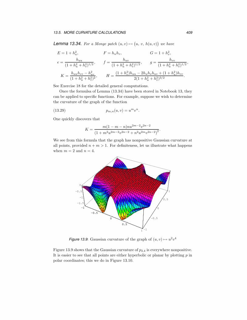
Lemma 13.34. For a Monge patch (u, v) 7→(

u, v, h(u, v))

we have

E = 1 + h2u, F = huhv, G = 1 + h2

v,

e =huu

(1 + h2u + h2

v)1/2

, f =huv

(1 + h2u + h2

v)1/2

, g =hvv

(1 + h2u + h2

v)1/2

,

K =huuhvv − h2

uv

(1 + h2u + h2

v)2, H =

(1 + h2v)huu − 2huhvhuv + (1 + h2

u)hvv

2(1 + h2u + h2

v)3/2

.

See Exercise 18 for the detailed general computations.

Once the formulsa of Lemma (13.34) have been stored in Notebook 13, they

can be applied to specific functions. For example, suppose we wish to determine

the curvature of the graph of the function

pm,n(u, v) = umvn.(13.29)

One quickly discovers that

K =m(1 −m− n)nu2m−2v2n−2

(1 +m2u2m−2v2n−2 + n2u2mv2n−2)2 .

We see from this formula that the graph has nonpositive Gaussian curvature at

all points, provided n+m > 1. For definiteness, let us illustrate what happens

when m = 2 and n = 4.

-1

-0.5

0

0.5

1-1

-0.5

0

0.5

1

-1.5

-1

-0.5

0

-1

-0.5

0

0.5

Figure 13.9: Gaussian curvature of the graph of (u, v) 7→ u2v4

Figure 13.9 shows that the Gaussian curvature of p2,4 is everywhere nonpositive.

It is easier to see that all points are either hyperbolic or planar by plotting p in

polar coordinates; this we do in Figure 13.10.


Figure 13.10: The graph of p2,4 in polar coordinates

13.6 A Global Curvature Theorem

We recall the following fundamental fact about compact subsets of Rn (see

page 373):

Lemma 13.35. Let R be a compact subset of Rn, and let f : R → R be a

continuous function. Then f assumes its maximum value at some point p ∈ R.

For a proof of this fundamental lemma, see [Buck, page 74].

Intuitively, it is reasonable that for each compact surface M ⊂ R3, there is

a point p0 ∈ M that is furthest from the origin, and at p0 the surface bends

towards the origin. Thus it appears that the Gaussian curvature K of M is

positive at p0. We now prove that this is indeed the case. The proof uses

standard facts from calculus concerning a maximum of a differentiable function

of one variable.

Theorem 13.36. If M is a compact regular surface in R3, there is a point

p ∈ R3 at which the Gaussian curvature K is strictly positive.

Proof. Let f : R3 → R be defined by f(p) = ‖p‖2. Then f is continuous (in

fact, differentiable), since it can be expressed in terms of the natural coordinate

functions of R3 as f = u2

1 + u22 + u2

3. By Lemma 13.35, f assumes its maximum

value at some point p0 ∈ M. Let v ∈ Mp be a unit tangent vector, and choose a

unit-speed curve α : (a, b) → M such that a < 0 < b, α(0) = p0 and α′(0) = v.

13.7. NONPARAMETRICALLY DEFINED SURFACES 411

Since the function g : (a, b) → R defined by g = f ◦ α has a maximum at 0, it

follows that

g′(0) = 0 and g′′(0) 6 0.

But g(t) = α(t) · α(t), so that

0 = g′(0) = 2α′(0) · α(0) = 2v · p0.(13.30)

In (13.30), v can be an arbitrary unit tangent vector, and so p0 must be normal

to M at p0. Clearly, p0 6= 0, so that (13.30) implies that p0/‖p0‖ is a unit

normal vector to M at p0. Furthermore,

0 > g′′(0) = 2α′′(0) · α(0) + 2α′(0) · α′(0) = 2(

α′′(0) · p0 + 1)

,

so that α′′(0) · p0 6 −1, or

k(v) = α′′(0) ·

p0

‖p0‖6 − 1

‖p0‖,(13.31)

where k(v) is the normal curvature determined by the tangent vector v and the

unit normal vector p0/‖p0‖. In particular, the principal curvatures of M at p0

(with respect to p0/‖p0‖) satisfy

k1(p0), k2(p0) 6 − 1

‖p0‖.

This implies that the Gaussian curvature of M at p0 satisfies

K(p0) = k1(p0)k2(p0) >1

‖p0‖2> 0.

Noncompact surfaces of positive Gaussian curvature exist (see Exercise 15).

On the other hand, for surfaces of negative curvature, we have the following

result (see Exercise 16):

Corollary 13.37. Any surface in R3 whose Gaussian curvature is everywhere

nonpositive must be noncompact.

13.7 Nonparametrically Defined Surfaces

So far we have discussed computing the curvature of a surface from its para-

metric representation. In this section we show how in some cases the curvature

can be computed from the nonparametric form of a surface.

Lemma 13.38. Let p be a point on a regular surface M ⊂ R3, and let vp and

wp be tangent vectors to M at p. Then the Gaussian and mean curvatures of

M at p are related to the shape operator by the formulas

S(vp) × S(wp) = K(p)vp × wp,(13.32)

S(vp) × wp + vp × S(wp) = 2H(p)vp × wp.(13.33)


Proof. First, assume that vp and wp are linearly independent. Then we can

write

S(vp) = avp + bwp and S(wp) = cvp + dwp,

so that(

a c

b d

)

is the matrix of S with respect to vp and wp. It follows from (13.19), page 398,

that

S(vp) × wp + vp × S(wp) = (avp + bwp) × wp + vp × (cvp + dwp)

= (a+ d)vp × wp

= (trS(p))vp × wp = 2H(p)vp × wp,

proving (13.33) in the case that vp and wp are linearly independent.

If vp and wp are linearly dependent, they are still the limits of linearly

independent tangent vectors. Since both sides of (13.33) are continuous in vp

and wp, we get (13.33) in the general case. equation (13.32) is proved by the

same method (see Exercise 22).

Theorem 13.39. Let Z be a nonvanishing vector field on a regular surface

M ⊂ R3 which is everywhere perpendicular to M. Let V and W be vector

fields tangent to M such that V × W = Z. Then

K =[Z DVZ DWZ]

‖Z‖4,(13.34)

H =[Z W DVZ] − [Z V DWZ]

2‖Z‖3.(13.35)

Proof. Let U = Z/‖Z‖; then (9.5), page 267, implies that

DVU =DVZ

‖Z‖ + V

[

1

‖Z‖

]

Z.

Therefore,

S(V) = −DVU =−DVZ

‖Z‖ + NV,

where NV is a vector field normal to M. By Lemma 13.38 we have

KV × W = S(V) × S(W)(13.36)

=

(−DVZ

‖Z‖ + NV

)

×(−DWZ

‖Z‖ + NW

)

.

13.7. NONPARAMETRICALLY DEFINED SURFACES 413

Since NV and NW are linearly dependent, it follows from (13.36) that

KZ =DVZ × DWZ

‖Z‖2+ some vector field tangent to M.

Taking the scalar product of both sides with Z yields (13.34). Equation (13.35)

is proved in a similar fashion.

In order to make use of Theorem 13.39, we need an important function that

measures the distance from the origin of each tangent plane to a surface.

Definition 13.40. Let M be an oriented regular surface in R3 with surface

normal U. Then the support function of M is the function h : M → R given by

h(p) = p · U(p).

Geometrically, h(p) is the distance from the origin to the tangent space Mp.

Corollary 13.41. Let M be the surface

{ (u1, u2, u3) ∈ R3 | f1uk

1 + f2uk2 + f3u

k3 = 1 },

where f1, f2, f3 are constants, not all zero, and k is a nonzero real number.

Then the support function, Gaussian curvature and mean curvature of M are

given by

h =1

√

f21u

2k−21 + f2

2u2k−22 + f2

3u2k−23

,(13.37)

K =(k − 1)2f1f2f3(u1u2u3)

k−2

( 3∑

i=1

f2i u

2k−2i

)2= h4(k − 1)2f1f2f3(u1u2u3)

k−2,(13.38)

H =−k + 1

2

( 3∑

i=1

f2i u

2k−2i

)3

2

(

f1f2(u1u2)k−2(f1u

k1 + f2u

k2)(13.39)

+f2f3(u2u3)k−2(f2u

k2 + f3u

k3) + f3f1(u3u1)

k−2(f3uk3 + f1u

k1))

.

Proof. Let g(u1, u2, u3) = f1uk1 + f2u

k2 + f3u

k3 − 1, so that

M = { p ∈ R3 | g(p) = 0 }.

Then Z = grad g is a nonvanishing vector field that is everywhere perpendicular

to M. Explicitly,

Z = k

3∑

i=1

fiuk−1i Ui,


u1, u2, u3 being the natural coordinate functions of R3, and Ui = ∂/∂ui (see

Definition 9.20). The vector field X =∑

uiUi satisfies

X · Z = k∑

fiuki ,(13.40)

in which the summations continue to be over i = 1, 2, 3. The support function

of M is given by

h = X ·

Z

‖Z‖ =

∑

fiuki

√

∑

f2i u

2k−2i

.

Since∑

fiuki equals 1 on M, we get (13.37).

Next, let

V =∑

viUi and W =∑

wiUi

be vector fields on R3. Since f1, f2, f3 are constants, we have

DVZ = k∑

V[fiuk−1i ]Ui = k(k − 1)

∑

fiviuk−2i Ui,

and similarly for W. Therefore, the triple product [Z DVZ DWZ] equals

det

kf1uk−11 kf2u

k−12 kf3u

k−13

k(k − 1)f1v1uk−21 k(k − 1)f2v2u

k−22 k(k − 1)f3v3u

k−23

k(k − 1)f1w1uk−21 k(k − 1)f2w2u

k−22 k(k − 1)f3w3u

k−23

= k3(k − 1)2f1f2f3uk−21 uk−2

2 uk−23 [X V W].

Now we choose V and W so that they are tangent to M and V × W = Z.

Using (13.34), we obtain

K =k3(k − 1)2f1f2f3u

k−21 uk−2

2 uk−23 X · Z

‖Z‖4=

(k − 1)2f1f2f3uk−21 uk−2

2 uk−23

( 3∑

i=1

f2i u

2k−2i

)2.

This proves (13.38). The proof of (13.39) is similar.

Computations in Notebook 13 yield three special cases of Corollary 13.41.

Corollary 13.42. The support function and Gaussian curvature of

(i) the ellipsoidx2

a2+y2

b2+z2

c2= 1,

(ii) the hyperboloid of one sheetx2

a2+y2

b2− z2

c2= 1,

(iii) the hyperboloid of two sheetsx2

a2− y2

b2− z2

c2= 1

13.8. EXERCISES 415

are given in each case by

h =

(

x2

a4+y2

b4+z2

c4

)−1/2

and K = ± h4

a2b2c2,

where the minus sign only applies in (ii).

We shall return to these quadrics in Section 19.6, where we describe geo-

metrically useful parametrizations of them. We conclude the present section by

considering a superquadric, which is a surface of the form

f1xk + f2y

k + f3zk = 1,

where k is different from 2. We do the special case k = 2/3, which is an astroidal

ellipsoid (see page 407).

Corollary 13.43. The Gaussian curvature of the superquadric

f1x2/3 + f2y

2/3 + f3z2/3 = 1

is given by

K =f1f2f3

9(

f23 (xy)2/3 + f2

2 (xz)2/3 + f21 (yz)2/3

)2 .

13.8 Exercises

M 1. Plot the graph of p2,3, defined by (13.29), and its Gaussian curvature.

M 2. Plot the following surfaces and describe in each case (without additional

calculation) the set of elliptic, hyperbolic, parabolic and planar points:

(a) a sphere,

(b) an ellipsoid,

(c) an elliptic paraboloid,

(d) a hyperbolic paraboloid,

(e) a hyperboloid of one sheet,

(f) a hyperboloid of two sheets.

This exercise continues on page 450.

3. By studying the plots of the surfaces listed in Exercise 2, describe the

general shape of the image of their Gauss maps.


4. Compute by hand the coefficients of the first fundamental form, those of

the second fundamental form, the unit normal, the mean curvature and

the principal curvatures of the following surfaces:

(a) the elliptical torus,

(b) the helicoid,

(c) Enneper’s minimal surface.

Refer to the exercises on page 377.

5. Compute the first fundamental form, the second fundamental form, the

unit normal, the Gaussian curvature, the mean curvature and the principal

curvatures of the patch

x(u, v) =(

u2 + v, v2 + u, uv)

.

6. The translation surface determined by curves α,γ : (a, b) → R3 is the patch

(u, v) 7→ α(u) + γ(v).

It is the surface formed by moving α parallel to itself in such a way that

a point of the curve moves along γ. Show that f = 0 for a translation

surface.

7. Explain the difference between the translation surface formed by a circle

and a lemniscate lying in perpendicular planes, and the twisted surface

formed from a lemniscate according to Section 11.6.

Figure 13.11: Translation and twisted surface formed by a lemniscate

8. Compute by hand the first fundamental form, the second fundamental

form, the unit normal, the Gaussian curvature, the mean curvature and

the principal curvatures of the patch

xn(u, v) =(

un, vn, uv).

For n = 3, see the picture on page 291.

13.8. EXERCISES 417

9. Prove the statement immediately following Definition 13.8.

10. Show that the first fundamental form of the Gauss map of a patch x

coincides with the third fundamental form of x.

11. Show that an orientation-preserving Euclidean motion F : R3 → R

3 leaves

unchanged both principal curvatures and principal vectors.

12. Show that the Bohemian dome defined by

bohdom[a, b, c, d](u, v) = (a cosu, b sinu+ c cos v, d sin v)

is the translation surface of two ellipses (see Exercise 6). Compute by hand

the Gaussian curvature, the mean curvature and the principal curvatures

of bohdom[a, b, b, a].

Figure 13.12: The Bohemian dome bohdom[1, 2, 2, 3]

13. Show that the mean curvature H(p) of a surface M ⊂ R3 at p ∈ M is

given by

H(p) =1

π

∫ π

0

k(θ)dθ,

where k(θ) denotes the normal curvature, as in the proof of Lemma 13.19.

14. (Continuation) Let n be an integer larger than 2 and for 0 6 i 6 n − 1,

put θi = ψ + 2πi/n, where ψ is some angle. Show that

H(p) =1

n

n−1∑

i=0

k(θi).


15. Give examples of a noncompact surface

(a) whose Gaussian curvature is negative,

(b) whose Gaussian curvature is identically zero,

(c) whose Gaussian curvature is positive,

(d) containing elliptic, hyperbolic, parabolic and planar points.

16. Prove Corollary 13.37 under the assumption that K is everywhere nega-

tive.

17. Show that there are no compact minimal surfaces in R3.

M 18. Find the coefficients the first, second and third fundamental forms to the

following surfaces:

(a) the elliptical torus defined on page 377,

(b) the helicoid defined on page 377,

(c) Enneper’s minimal surface defined on page 378,

(d) a Monge patch defined on page 302.

19. Determine the principal curvatures of the Whitney umbrella. Its mean

curvature is shown in Figure 13.13.

-0.1

-0.05

0

0.05

0.10.01

0.011

0.012

0.013

0.014

0.015

-1000

-500

0

500

1000

-0.1

-0.05

0

0.05

Figure 13.13: Gaussian curvature of the Whitney umbrella

13.8. EXERCISES 419

M 20. Find the formulas for the coefficients e, f, g of the second fundamental

forms of the following surfaces parametrized in Chapter 11: the Mobius

strip, the Klein bottle, Steiner’s Roman surface, the cross cap.

M 21. Find the formulas for the Gaussian and mean curvatures of the surfaces

of the preceding exercise.

22. Prove equation (13.32).

23. Prove

Lemma 13.44. Let M ⊂ R3 be a surface, and suppose that x : U → M

and y : V → M are coherently oriented patches on M with x(U) ∩ y(V)

nonempty. Let x−1 ◦ y = (u, v): U ∩ V → U ∩ V be the associated change

of coordinates, so that

y(u, v) = x(

u(u, v), v(u, v))

.

Let ex, fx, gx denote the coefficients of the second fundamental form of x,

and let ey, fy, gy denote the coefficients of the second fundamental form

of y. Then

ey = ex

(

∂u

∂u

)2

+ 2fx∂u

∂u

∂v

∂u+ gx

(

∂v

∂u

)2

,

fy = ex∂u

∂u

∂u

∂v+ fx

(

∂u

∂u

∂v

∂v+∂u

∂v

∂v

∂u

)

+ gx∂v

∂u

∂v

∂v,

gy = ex

(

∂u

∂v

)2

+ 2fx∂u

∂v

∂v

∂v+ gx

(

∂v

∂v

)2

.

(13.41)

24. Prove equation (13.39) of Corollary 13.41.

Documents

Shape and Curvature - unito.itwebmath2.unito.it/paginepersonali/sergio.console/CurveSuperfici/AG13.pdf · Chapter 13 Shape and Curvature In this chapter, we study the relationship