FAKULTI KEJURUTERAAN ELEKTRONIK & KEJURUTERAAN …myweb.utem.edu.my/myweb/amat/downloads/BEKG2323/Chapter2.pdf · Obtaining system’s schematic (block diagram) Develop mathematical

1

SUBJECT : CONTROL PRINCIPLES BEKG 2323 FFAAKKUULLTTII KKEEJJUURRUUTTEERRAAAANN EELLEEKKTTRROONNIIKK && KKEEJJUURRUUTTEERRAAAANN KKOOMMPPUUTTEERR

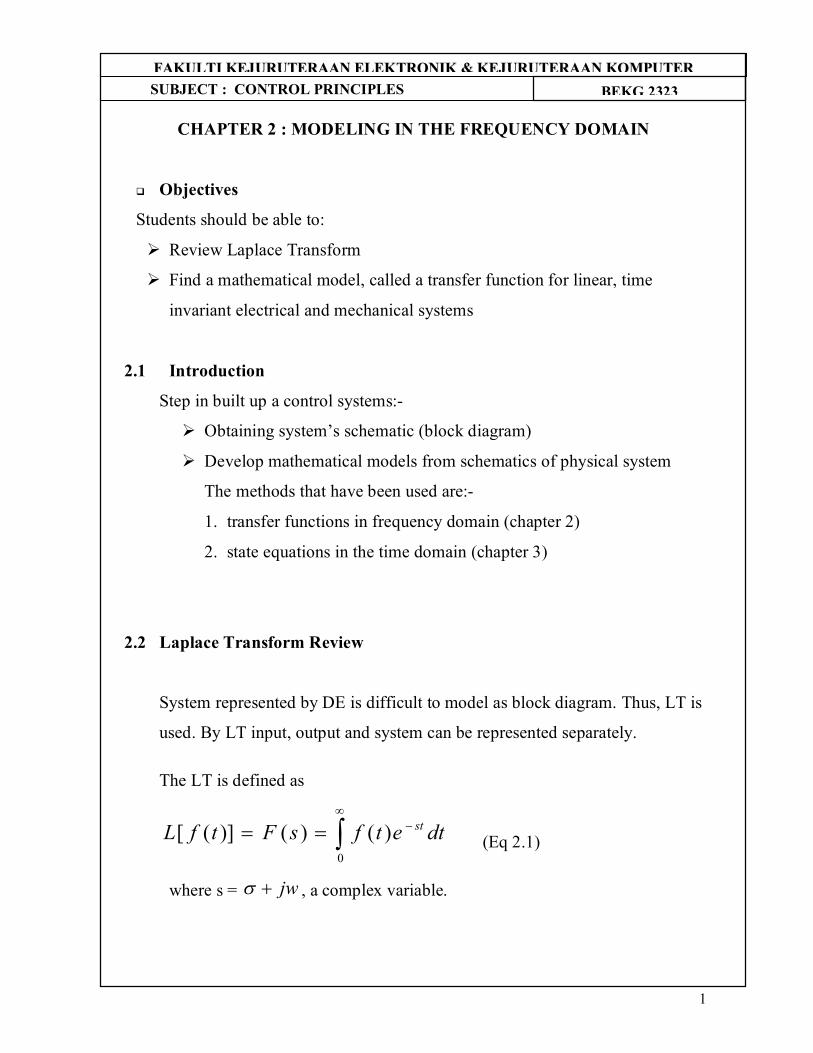
CHAPTER 2 : MODELING IN THE FREQUENCY DOMAIN

Objectives

Students should be able to:

Review Laplace Transform

Find a mathematical model, called a transfer function for linear, time

invariant electrical and mechanical systems

2.1 Introduction

Step in built up a control systems:-

Obtaining system’s schematic (block diagram)

Develop mathematical models from schematics of physical system

The methods that have been used are:-

1. transfer functions in frequency domain (chapter 2)

2. state equations in the time domain (chapter 3)

2.2 Laplace Transform Review

System represented by DE is difficult to model as block diagram. Thus, LT is

used. By LT input, output and system can be represented separately.

The LT is defined as

0

)()()]([ dtetfsFtfL st (Eq 2.1)

where s = jw , a complex variable.

2


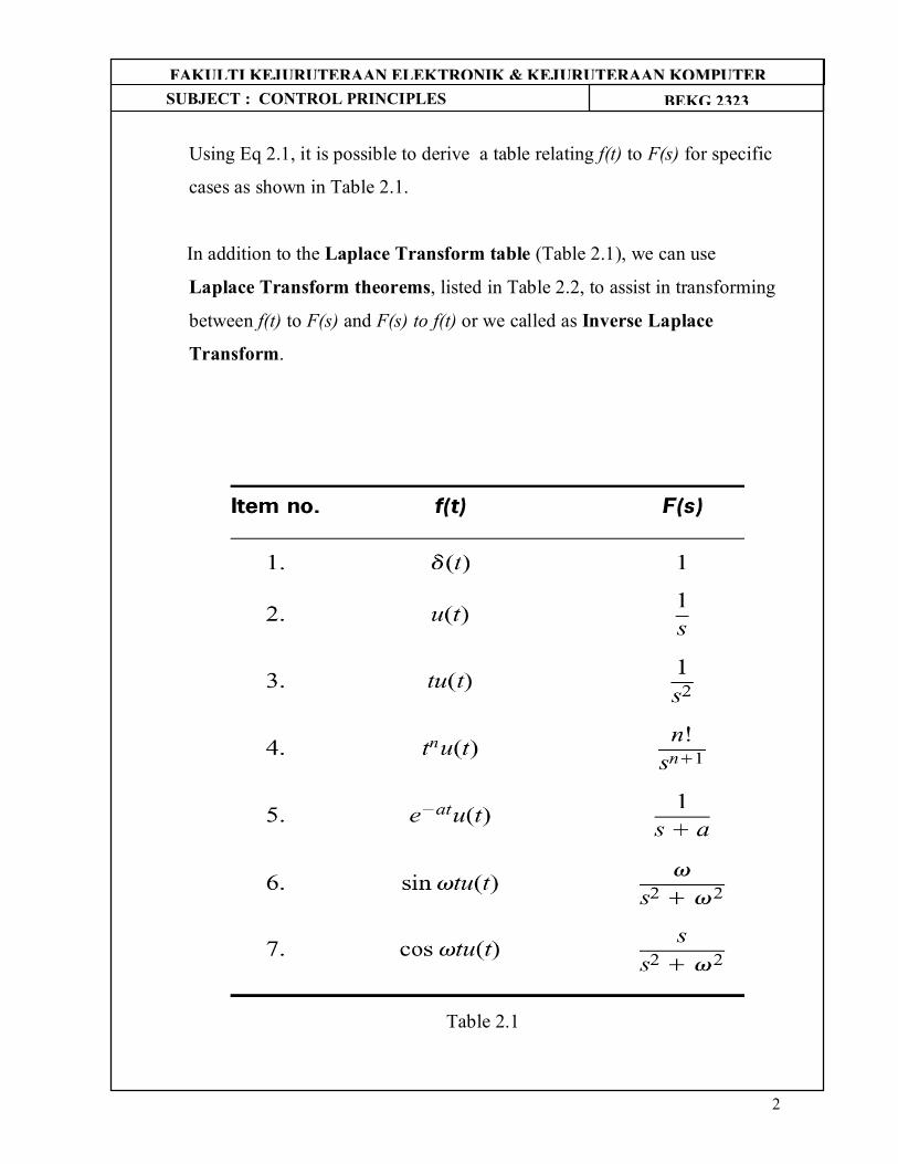
Using Eq 2.1, it is possible to derive a table relating f(t) to F(s) for specific

cases as shown in Table 2.1.

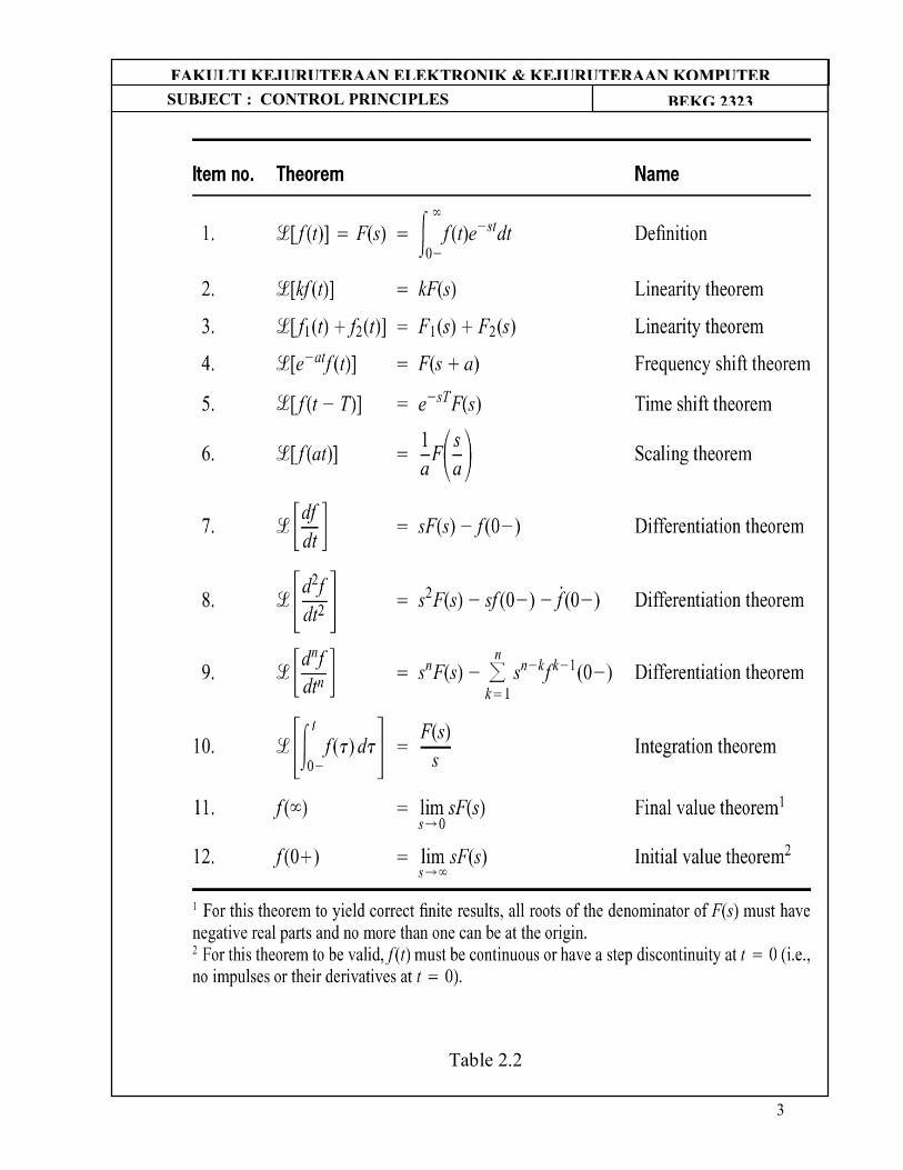
In addition to the Laplace Transform table (Table 2.1), we can use

Laplace Transform theorems, listed in Table 2.2, to assist in transforming

between f(t) to F(s) and F(s) to f(t) or we called as Inverse Laplace

Transform.

Table 2.1

3


Table 2.2

4


Ex 2.1

Find the Laplace transform of f(t) = Ae-atu(t).

Answer : F(s) = asA

Ex 2.2

Find the Laplace tranform of ydtdy

dtyd

dtydty 453)( 2

2

3

3

Answer : Y(s) = s3Y(s) + 3s2Y(s) + 5sY(s) + 4 Y(s)

Ex 2.3

Find the inverse Laplace transform of F(s) = 1/(s+3)2

Answer : f(t) = e-3ttu(t)

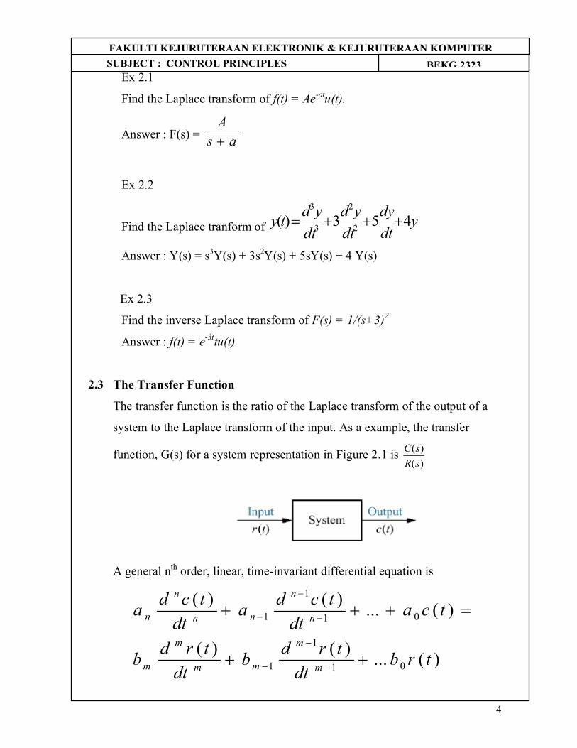
2.3 The Transfer Function

The transfer function is the ratio of the Laplace transform of the output of a

system to the Laplace transform of the input. As a example, the transfer

function, G(s) for a system representation in Figure 2.1 is )()(

sRsC

A general nth order, linear, time-invariant differential equation is

)(...)()(

)(...)()(

01

1

1

01

1

1

trbdt

trdbdt

trdb

tcadt

tcdadt

tcda

m

m

mm

m

m

n

n

nn

n

n

5


where : c(t) is output

r(t) is input

a and b are constants

Taking Laplace transform of both side,

ansnC(s) + an-1sn-1C(s) +… + a0C(s) + initial condition =

bmsmR(s) + bm-1sm-1R(s) +… + b0R(s) + initial condition

Assume all initial conditions are zero,

(ansn + an-1sn-1 +… + a0) C(s) = (bmsm + bm-1sm-1 +… + b0) R(s)

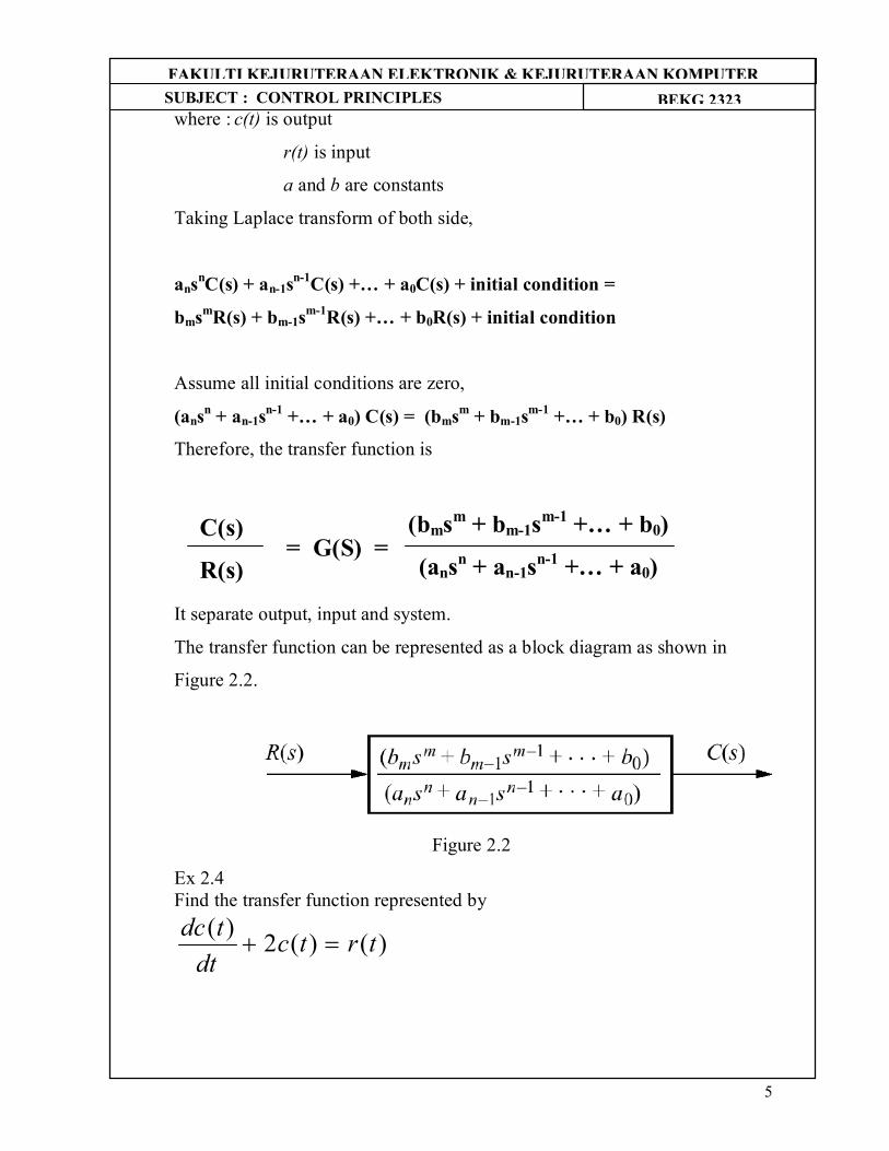
Therefore, the transfer function is

It separate output, input and system.

The transfer function can be represented as a block diagram as shown in

Figure 2.2.

Figure 2.2

Ex 2.4 Find the transfer function represented by

)()(2)( trtcdt

tdc

(bmsm + bm-1sm-1 +… + b0)

(ansn + an-1sn-1 +… + a0) = G(S) =

C(s)

R(s)

6


Sol Taking LT both side (refer Table 2.1 and 2.2), and assume zero initial condition

2s1

R(s)C(s)G(s)

R(s)2C(s)sC(s)

Ex 2.5 Use the results of ex 2.4 to find the response, c(t) to an input r(t)=u(t), a unit step. Assume zero initial condition.

Answer: tetc 2

21

21)(

Ex 2.6 Find the transfer function, G(s) corresponding to differential equation

rdtdr

dtrdc

dtdc

dtcd

dtcd 34573 2

2

2

2

3

3

Answer

57s3ss34ssG(s) 23

2

Ex 2.7 Find the differential equation corresponding to the transfer function.

2612)( 2

ssssG

Answer

)()(2)(2)(6)(2

2

trdt

tdrtcdt

tdcdt

tcd

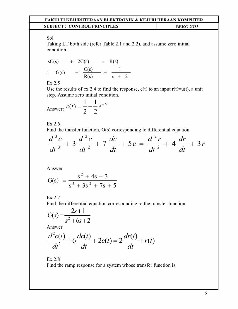
Ex 2.8 Find the ramp response for a system whose transfer function is

7


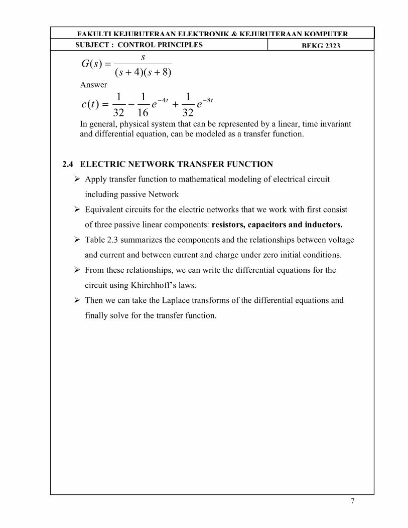
)8)(4()(

ssssG

Answer

tt eetc 84

321

161

321)(

In general, physical system that can be represented by a linear, time invariant and differential equation, can be modeled as a transfer function.

2.4 ELECTRIC NETWORK TRANSFER FUNCTION

Apply transfer function to mathematical modeling of electrical circuit

including passive Network

Equivalent circuits for the electric networks that we work with first consist

of three passive linear components: resistors, capacitors and inductors.

Table 2.3 summarizes the components and the relationships between voltage

and current and between current and charge under zero initial conditions.

From these relationships, we can write the differential equations for the

circuit using Khirchhoff’s laws.

Then we can take the Laplace transforms of the differential equations and

finally solve for the transfer function.

8


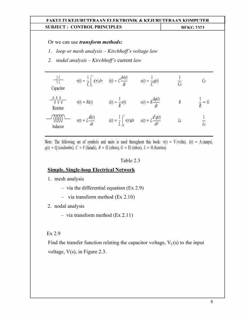
Or we can use transform methods:

1. loop or mesh analysis – Kirchhoff’s voltage law

2. nodal analysis – Kirchhoff’s current law

Table 2.3

Simple, Single-loop Electrical Network

1. mesh analysis

– via the differential equation (Ex 2.9)

– via transform method (Ex 2.10)

2. nodal analysis


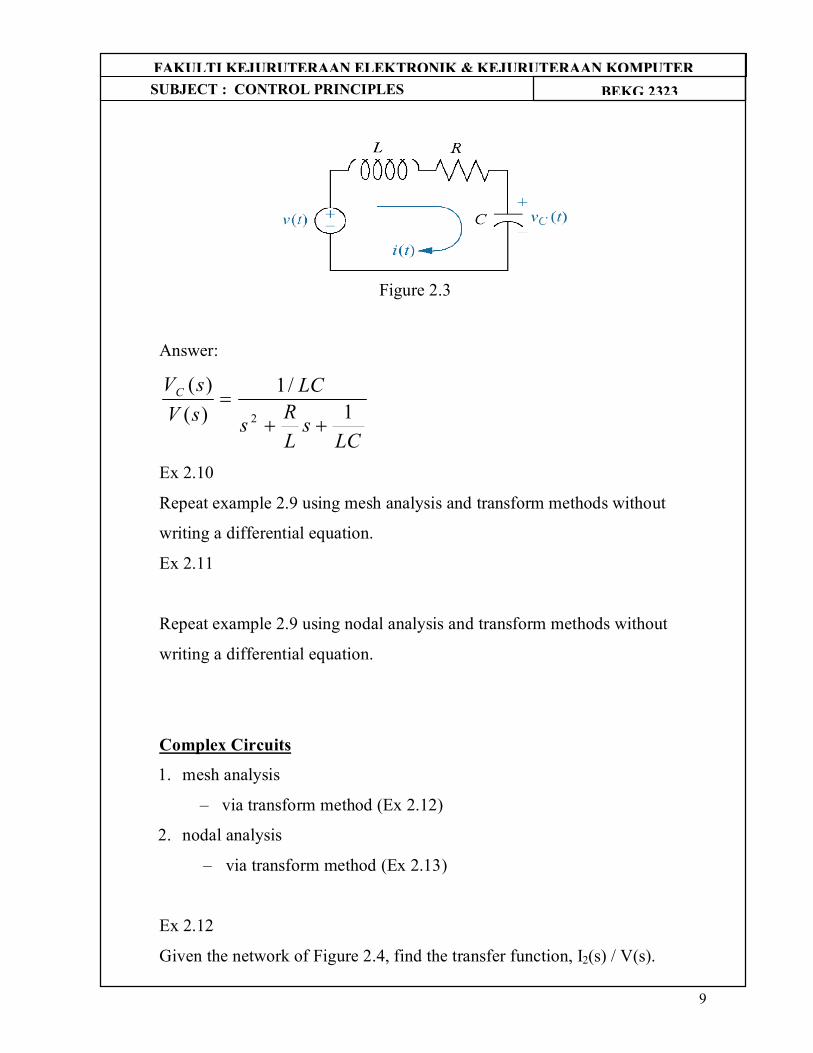
Ex 2.9

Find the transfer function relating the capacitor voltage, VC(s) to the input

voltage, V(s), in Figure 2.3.

9


Figure 2.3

Answer:

LCs

LRs

LCsVsVC

1/1

)()(

2

Ex 2.10

Repeat example 2.9 using mesh analysis and transform methods without

writing a differential equation.

Ex 2.11

Repeat example 2.9 using nodal analysis and transform methods without

writing a differential equation.

Complex Circuits

1. mesh analysis


2. nodal analysis


Ex 2.12

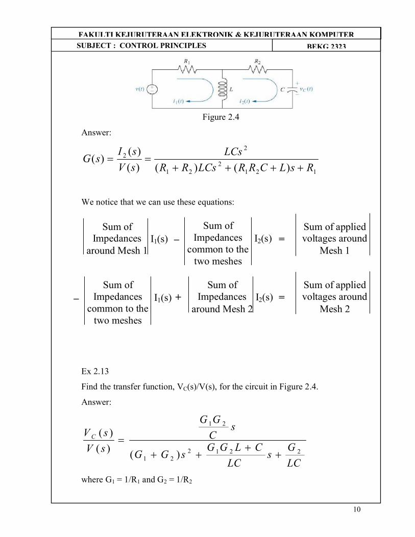
Given the network of Figure 2.4, find the transfer function, I2(s) / V(s).

10


Figure 2.4

Answer:

1212

21

22

)()()()()(

RsLCRRLCsRRLCs

sVsIsG

We notice that we can use these equations:

Ex 2.13

Find the transfer function, VC(s)/V(s), for the circuit in Figure 2.4.

Answer:

LCGs

LCCLGGsGG

sCGG

sVsV C

221221

21

)()()(

where G1 = 1/R1 and G2 = 1/R2

Sum of Impedances

around Mesh 1 I1(s) _

Sum of Impedances

common to the two meshes

I2(s) = Sum of applied voltages around

Mesh 1

Sum of Impedances

around Mesh 2 I2(s) _

Sum of Impedances

common to the two meshes

I1(s) = Sum of applied voltages around

Mesh 2 +

11


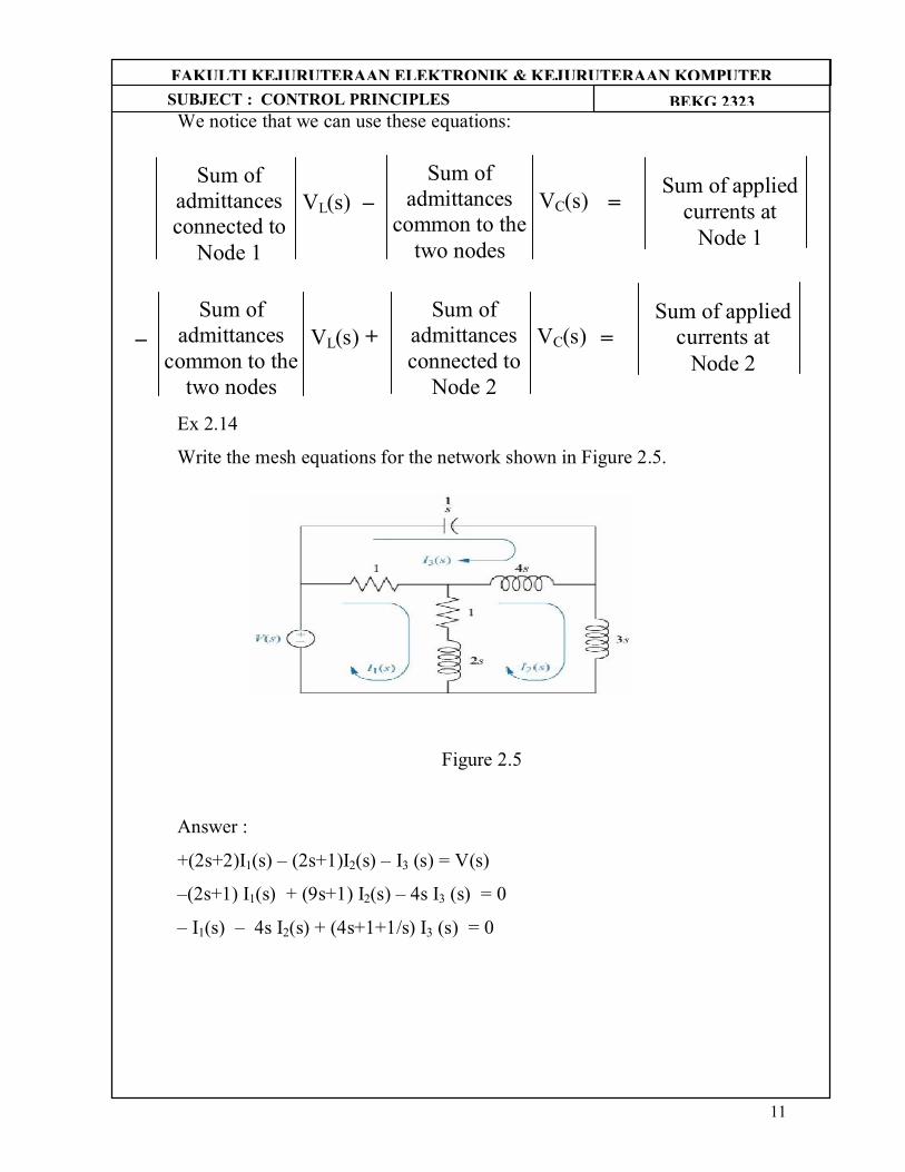
We notice that we can use these equations:

Ex 2.14

Write the mesh equations for the network shown in Figure 2.5.

Figure 2.5

Answer :

+(2s+2)I1(s) – (2s+1)I2(s) – I3 (s) = V(s)

–(2s+1) I1(s) + (9s+1) I2(s) – 4s I3 (s) = 0

– I1(s) – 4s I2(s) + (4s+1+1/s) I3 (s) = 0

Sum of admittances connected to

Node 1

VL(s) _ Sum of

admittances common to the

two nodes

VC(s) = Sum of applied

currents at Node 1

Sum of admittances connected to

Node 2

VC(s) _ Sum of

admittances common to the

two nodes

VL(s) = Sum of applied

currents at Node 2

+

12


2.5 TRANSLATIONAL MECHANICAL SYSTEM TRANSFER

FUNCTIONS

We have shown that electrical networks can be modeled by a transfer

function.

Now we will do the same for mechanical systems.

Mechanical systems, like electrical network, can be have 3 passive, linear

components. Two of them, the spring and the mass, are energy-storage

elements; and one of them, the viscous damper, dissipates energy.

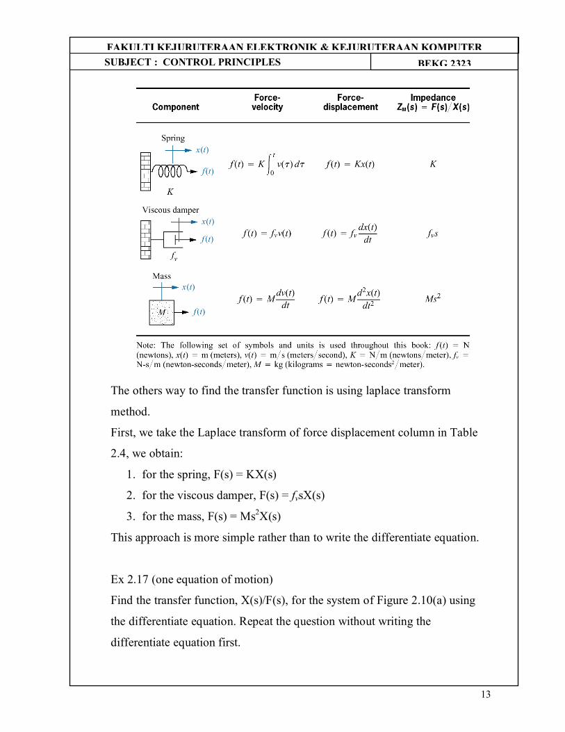
These mechanical elements are shown in Table 2.4.

In the table, K, fv and M are called spring constant, coefficient of viscous

friction and mass, respectively.

We now create analogies between electrical and mechanical systems by

comparing Table 2.3 and 2.4.

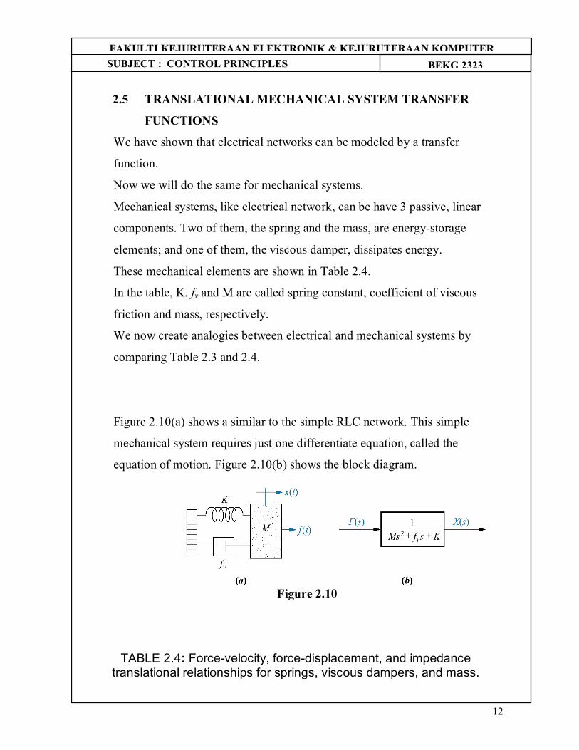
Figure 2.10(a) shows a similar to the simple RLC network. This simple

mechanical system requires just one differentiate equation, called the

equation of motion. Figure 2.10(b) shows the block diagram.

Figure 2.10

TABLE 2.4: Force-velocity, force-displacement, and impedance translational relationships for springs, viscous dampers, and mass.

13


The others way to find the transfer function is using laplace transform

method.

First, we take the Laplace transform of force displacement column in Table

2.4, we obtain:

1. for the spring, F(s) = KX(s)

2. for the viscous damper, F(s) = fvsX(s)

3. for the mass, F(s) = Ms2X(s)

This approach is more simple rather than to write the differentiate equation.

Ex 2.17 (one equation of motion)

Find the transfer function, X(s)/F(s), for the system of Figure 2.10(a) using

the differentiate equation. Repeat the question without writing the

differentiate equation first.

14


Answer:

KsfMssFsX

v 2

1)()(

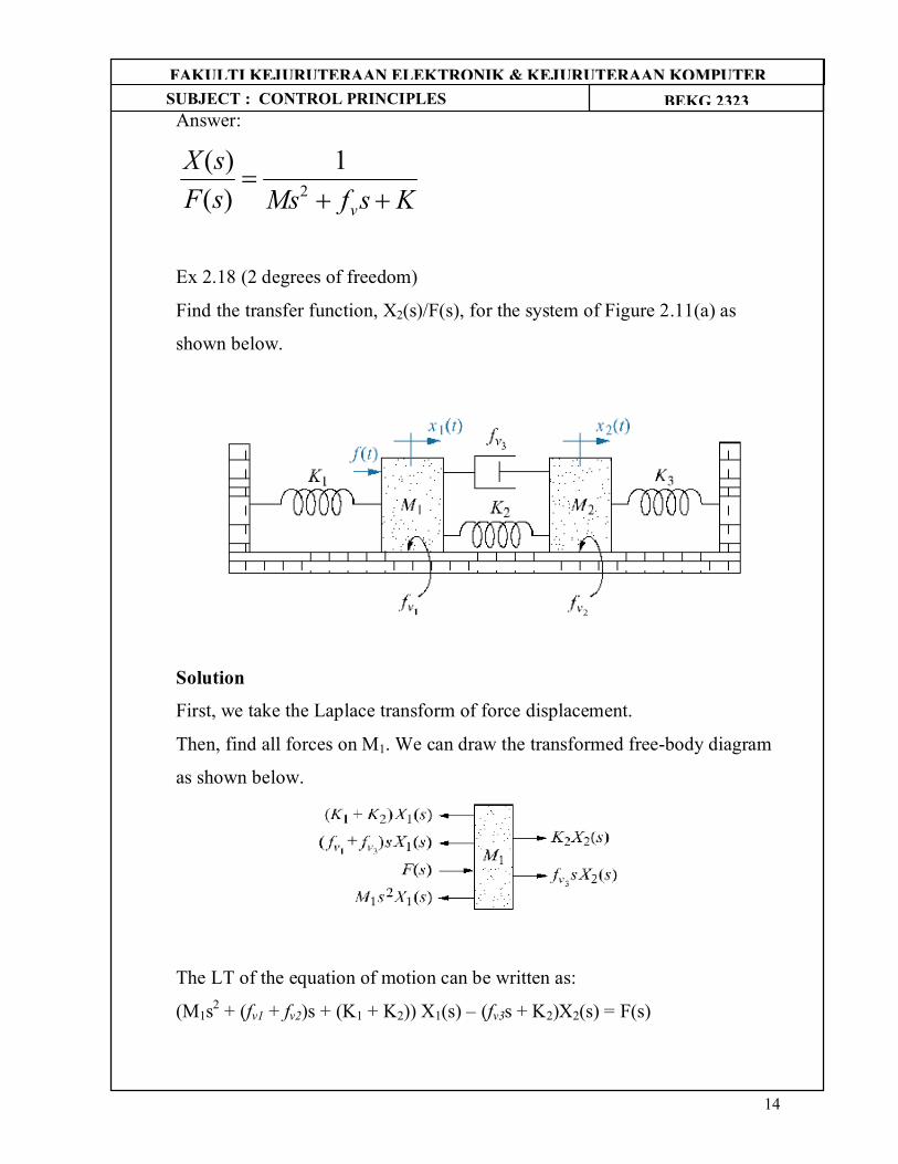
Ex 2.18 (2 degrees of freedom)

Find the transfer function, X2(s)/F(s), for the system of Figure 2.11(a) as

shown below.

Figure 2.11

Solution

First, we take the Laplace transform of force displacement.

Then, find all forces on M1. We can draw the transformed free-body diagram

as shown below.

The LT of the equation of motion can be written as:

(M1s2 + (fv1 + fv2)s + (K1 + K2)) X1(s) – (fv3s + K2)X2(s) = F(s)

15


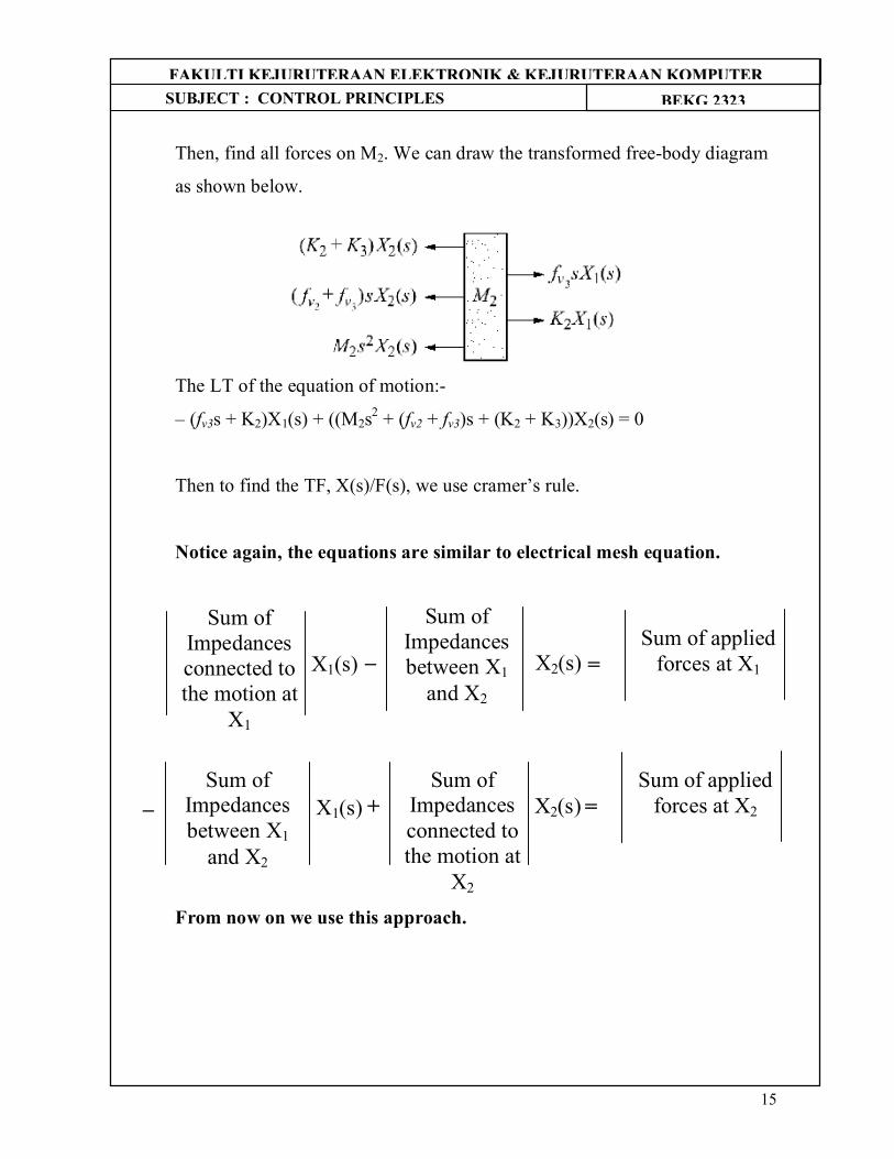
Then, find all forces on M2. We can draw the transformed free-body diagram

as shown below.

The LT of the equation of motion:-

– (fv3s + K2)X1(s) + ((M2s2 + (fv2 + fv3)s + (K2 + K3))X2(s) = 0

Then to find the TF, X(s)/F(s), we use cramer’s rule.

Notice again, the equations are similar to electrical mesh equation.

From now on we use this approach.

Sum of Impedances connected to the motion at

X1

X1(s) _

Sum of Impedances between X1

and X2

X2(s) = Sum of applied

forces at X1

_ Sum of

Impedances connected to the motion at

X2

X2(s) Sum of

Impedances between X1

and X2

X1(s) = Sum of applied

forces at X2 +

16


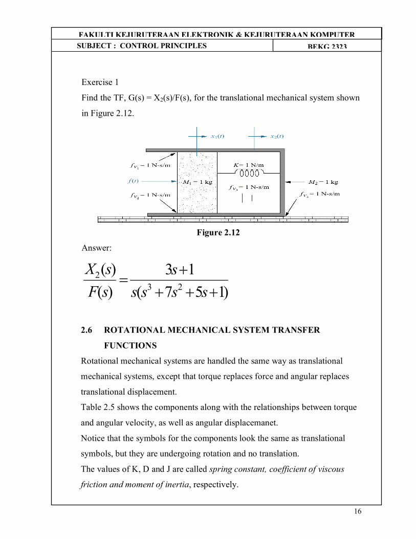
Exercise 1

Find the TF, G(s) = X2(s)/F(s), for the translational mechanical system shown

in Figure 2.12.

Figure 2.12

Answer:

)157(13

)()(

232

ssss

ssFsX

2.6 ROTATIONAL MECHANICAL SYSTEM TRANSFER

FUNCTIONS

Rotational mechanical systems are handled the same way as translational

mechanical systems, except that torque replaces force and angular replaces

translational displacement.

Table 2.5 shows the components along with the relationships between torque

and angular velocity, as well as angular displacemanet.

Notice that the symbols for the components look the same as translational

symbols, but they are undergoing rotation and no translation.

The values of K, D and J are called spring constant, coefficient of viscous

friction and moment of inertia, respectively.

17


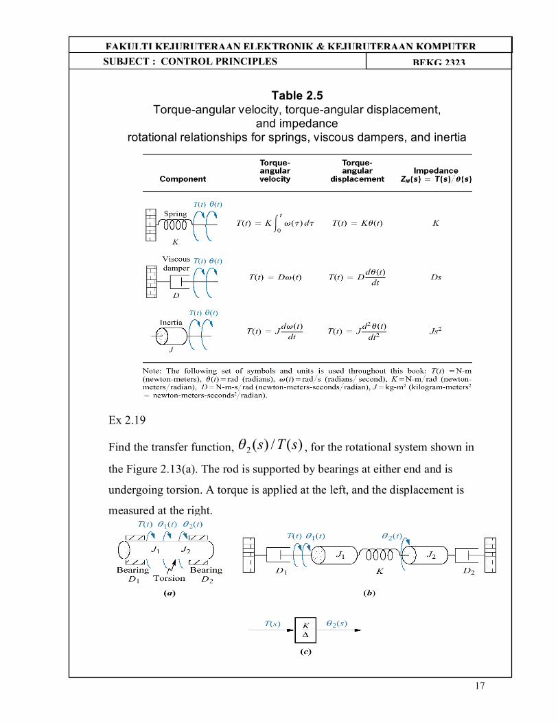
Table 2.5 Torque-angular velocity, torque-angular displacement,

and impedance rotational relationships for springs, viscous dampers, and inertia

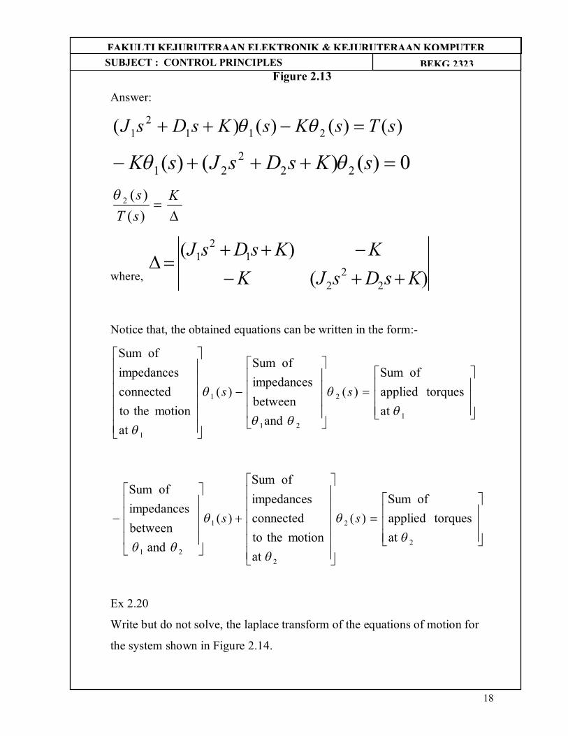
Ex 2.19

Find the transfer function, )(/)(2 sTs , for the rotational system shown in

the Figure 2.13(a). The rod is supported by bearings at either end and is

undergoing torsion. A torque is applied at the left, and the displacement is

measured at the right.

18


Figure 2.13

Answer:

)()()()( 2112

1 sTsKsKsDsJ

0)()()( 222

21 sKsDsJsK

KsTs)()(2

where, )()(

22

2

12

1

KsDsJKKKsDsJ

Notice that, the obtained equations can be written in the form:-

1

2

21

1

1

at torquesapplied

of Sum)(

andbetweenimpedances

of Sum

)(

at motion theto

connectedimpedances

of Sum

ss

2

2

2

1

21

at torquesapplied

of Sum)(

at motion theto

connectedimpedances

of Sum

)(

and betweenimpedances

of Sum

ss

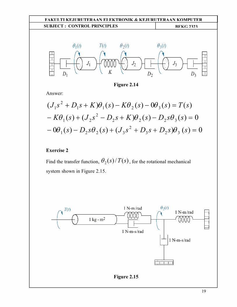
Ex 2.20

Write but do not solve, the laplace transform of the equations of motion for

the system shown in Figure 2.14.

19


Figure 2.14

Answer:

0)()()()(0

0)()()()(

)()(0)()()(

3232

3221

32222

21

32112

1

ssDsDsJssDs

ssDsKsDsJsKsTssKsKsDsJ

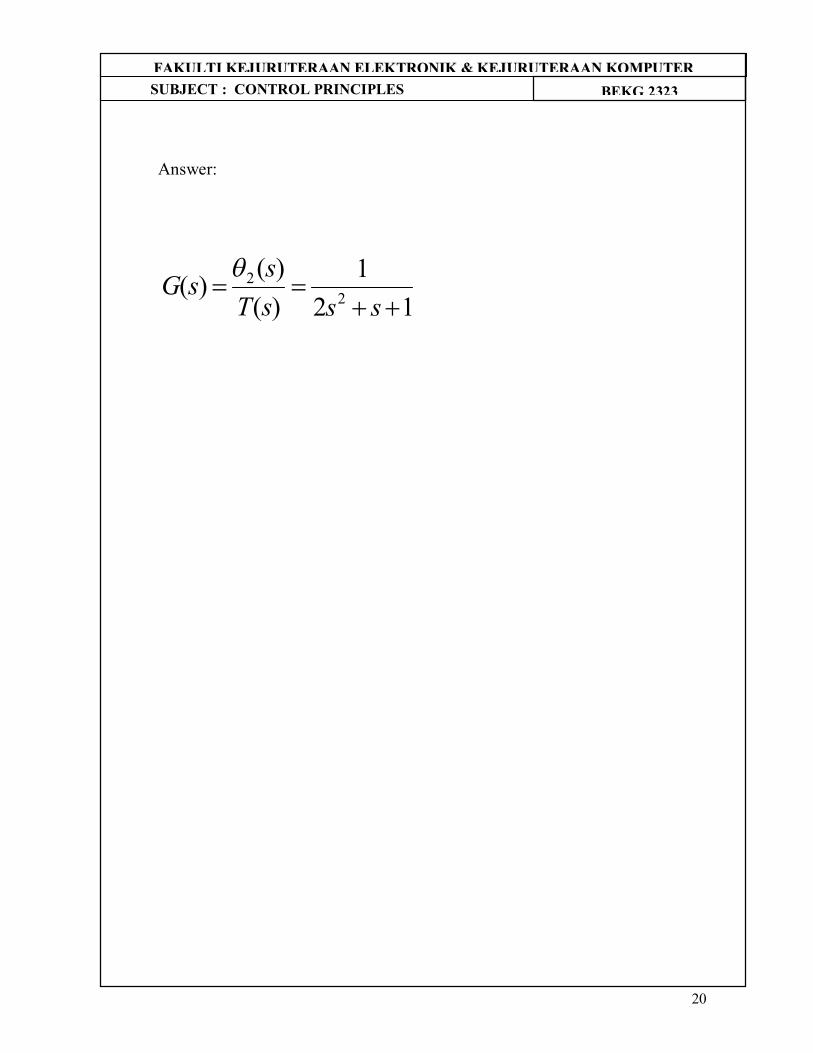
Exercise 2

Find the transfer function, )(/)(2 sTs , for the rotational mechanical

system shown in Figure 2.15.

Figure 2.15

20


Answer:

121

)()(

)( 22

sssTs

sG

Documents

FAKULTI KEJURUTERAAN ELEKTRONIK & KEJURUTERAAN …myweb.utem.edu.my/myweb/amat/downloads/BEKG2323/Chapter2.pdf · Obtaining system’s schematic (block diagram) Develop mathematical