FACTORS AFFECTING PROFITABILITY OF SMALL SCALE · PDF file · 2018-01-12Factors Affecting Profitability of Small Scale Farming 2 tendency of firms to cluster, either because of the

International Journal of Food and Agricultural Economics

ISSN 2147-8988

Vol. 2 No. 3 pp. 1-18

1

FACTORS AFFECTING PROFITABILITY OF SMALL SCALE

FARMING IN SOUTHERN TRINIDAD & TOBAGO

Hazel Patterson-Andrews

Department of Agricultural Economics and Extension, The University of the

West Indies, St Augustine

Carlisle A. Pemberton Department of Agricultural Economics and Extension, The University of the

West Indies, St Augustine, E-mail: [email protected], Tel: 868 662

2002 ext 82308

Abstract

This study examined several possible factors determining the profitability of small scale

crop farmers in Trinidad and Tobago in the Caribbean. Industrial/urban influence on profit

efficiency was tested by the creation of a special variable (IFOUR). This variable along with

farming and socio-economic variables were incorporated into a translog augmented

stochastic profit frontier. The significance of coefficients was tested as well as the

calculation of the elasticity of profit with respect to the wage rate. The study found a

significant negative impact of wage rates on profitability. Also the age of the farmer

negatively affected profitability, while the number of years farming had a positive effect. This

latter variable also significantly influenced both the one-sided error and idiosyncratic error

terms. However IFOUR measuring industrial/urban influence did not significantly affect the

profitability. The farmers had a mean profit efficiency of 48.4%, which was low in

international comparisons.

Key Word: Caribbean Farming, Stochastic Profit Frontier

1. Introduction

Low farm profitability is a major concern of developing countries because of concerns

for its effects on food security, by limiting the supply of food and the access to food by rural

households because of low farm incomes (Aung, 2011; Liverpool-Tasie, Kuku & Ajibola,

2011 pp. 6-24). Food security concerns have developed because of recent food shortages and

high food prices. Several factors have been offered for these recent developments, including

increased demand for food grains and oil seeds for fuel production, increasing prices for

these commodities, the weak US dollar, the increase in farm production costs due to higher

energy prices and droughts (Mitchell, 2008). However this article focuses on low farm

profitability in an industrializing, developing country and in small scale crop farming and its

possible causes such as high input prices, especially for labour and other socio-economic

factors.

Industrialization, the development of manufacturing industry and mineral resource

extraction, has long been favoured as the vehicle for economic growth of tropical countries,

since it tends to create economic activity of higher productivity (UNIDO, 2008).

Industrialization generally concentrates in specific geographical areas, because of the

mailto:[email protected]

Factors Affecting Profitability of Small Scale Farming…

2

tendency of firms to cluster, either because of the location of the extractable mineral

resource, or because of agglomeration economies in manufacturing. These economies are

associated with access to a pool of specialised workers and quick access to supplies of inputs

and knowledge relevant to the manufacturing firms (UNIDO, 2008).

Because of the concentration of activity geographically, industrialisation leads to issues

associated with urbanisation - the growth in size, social and economic influence of towns and

cities, especially into surrounding rural areas. These issues include the formation of slums,

the spread of disease, gang violence, pollution etc. Industrialization can also have a major

impact on employment creation, both formal and informal, as well as on the increase in

labour wage rates. It can also cause an increase in the rental value of land within its specific

geographical area of influence, as well as provide an expanding market for food produced in

proximal areas.

Several studies have examined the industrialization of agriculture and the food sector. For

example, Sexton (2000) examined the implications for competition and welfare of the

industrialization and consolidation in the U.S. food sector. Sonka (2003) examined the

implications for the grain industry in the US, while Molnar, Hoban, Parrish, and Futreal

(1997) examined the trends and spatial patterns of agricultural industrialization and the

implications for field-level work by the Natural Resources Conservation Service of the

USDA. However fewer studies have examined the possible impact of industrialization in the

economy as a whole, on the agricultural sector. Hyami (1969) argued for example that, based

on international comparisons and the analysis of the Japanese experience, industrialization

may promote agricultural development, by improving the conditions of supply of modern

inputs to agriculture. He used this argument to explain the observation that the agricultural

productivity of less developed countries, whose comparative advantage seems to lie in

agriculture grew slowly, relative to agriculture in developed countries. On the other hand,

Henneberry, Khan, and Piewthongngam (2000) based on an analysis of Pakistan's industrial

and agricultural sectors, concluded that while the sectors are complementary, “industry tends

to benefit more from agricultural growth than vice versa”.

What this study proposes is that the “industrial/urban influence” (consisting of the

proximity to an industrial centre and the population density of the area in which the farm is

located) can affect farm profitability directly as well as through labour wage rates and family

labour utilization. This article examined the effects of these factors, as well as other farm and

farmer related characteristics on the profitability of small scale farming in an expanding

industrial area in southern Trinidad and Tobago, a small island nation in the Caribbean.

A major location of industrialisation in Trinidad and Tobago is the southern area of Point

Fortin on the island of Trinidad. Point Fortin was the first centre of oilfield operations in

Trinidad and has been described as “the town that oil built” growing up in the space of 50

years from 1907, “from a forest clearing to a modern town of 30,000 people” (Brereton

1982). Since 1999, there has been another surge in industrialisation in Point Fortin as the

Liquefied Natural Gas (LNG) industrial plants are located there. Atlantic LNG Company,

produces LNG from natural gas delivered from fields in and around Trinidad and Tobago,

and is the seventh largest LNG producer in the world, and the largest such producer in the

Western Hemisphere. The company occupies a significant position in the local energy

industry, as it is the largest single contributor to Trinidad and Tobago’s exports and a

significant contributor to the country’s gross domestic product (GDP). Its annual production

represents more than half of the economic contribution of the entire refining sector. The area

around Point Fortin formed the location of this study.

The next section presents the conceptual framework of the study which is followed by the

empirical procedures used.

H.P. Andrews and C. Pemberton

3

2. Conceptual Framework

Models of urban influence provide a useful point of departure for developing a theoretical

framework for this study, (for example, Levanis, 2005), and this approach is therefore

adopted. We assume,

An industrial centre which provides a market for small farmers located at increasing

distances, , from the centre

Each small farmer rents an acreage of land A, which is devoted to production of

one crop

Farmers utilize hired labour, x, obtained at a price w. Part of the labour input,

family labour, may be fixed in the short run. Family labour may include those “disguisedly

employed” with marginal productivity close to zero or even negative (Lewis, 1954).

Each small farmer produces one crop which is chosen according to the demands of

the market at the industrial centre, as well as the edaphic and topographical conditions of the

farm.

The small farmer maximizes profits, , subject to the constraint of an implicit

production function, F (y*, x, A) = 0, where y* is the fixed level of the crop produced

The farmer’s use of technology is affected by a number of socioeconomic factors

including the farmer’s age, gender, and educational attainment.

The average cost of transporting the crop produced to the industrial centre is , with

being a positive function of distance – the further away from the industrial centre the

greater the transportation cost.

The small farmer sells the constrained crop output y* at the industrial centre at a

price p, but the farmer receives a net price [ τ(δ)]p because of the transportation costs

)( to the market and 0)(

Land at the industrial centre has an annual rental value per acre of VI and this annual

rental declines exponentially with distance from the centre at rate -.

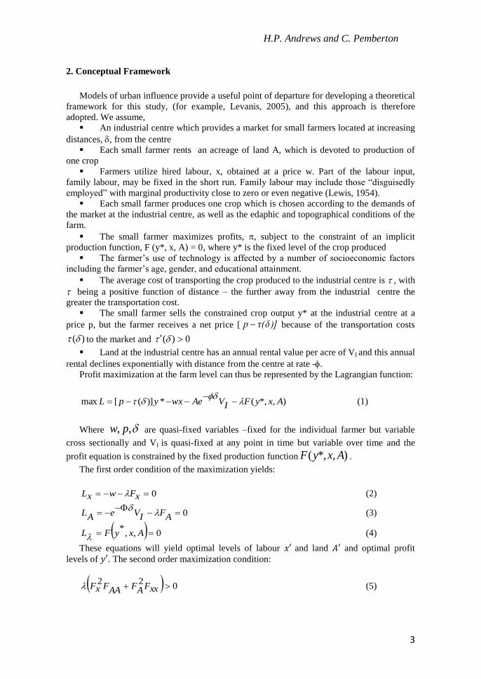
Profit maximization at the farm level can thus be represented by the Lagrangian function:

),*,(*)]([max AxyFIVAewxypL

(1)

Where ,, pw are quasi-fixed variables –fixed for the individual farmer but variable

cross sectionally and VI is quasi-fixed at any point in time but variable over time and the

profit equation is constrained by the fixed production function ),*,( AxyF .

The first order condition of the maximization yields:

0 xFwxL

(2)

0

AFIVeAL

(3)

0,,*

AxyFL (4)

These equations will yield optimal levels of labour and land and optimal profit

levels of . The second order maximization condition:

022

xxFAFAAFxF

(5)


4

imposes no constraint on the sign of FA or Fx. We therefore assume Fx > 0 and FA > 0.

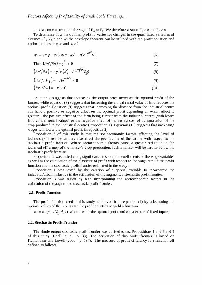
To determine how the optimal profit varies for changes in the quasi fixed variables of

distance , V1, p and w, the envelope theorem can be utilized with the profit equation and

optimal values of x, x′ and A, A′.

1*)(* VeAxwypy

(6)

Then 0* yp (7)

1*

VAey

(8)

01

AeV (9)

0 xw (10)

Equation 7 suggests that increasing the output price increases the optimal profit of the

farmer, while equation (9) suggests that increasing the annual rental value of land reduces the

optimal profit. Equation (8) suggests that increasing the distance from the industrial centre

can have a positive or negative effect on the optimal profit depending on which effect is

greater – the positive effect of the farm being further from the industrial centre (with lower

land annual rental values) or the negative effect of increasing cost of transportation of the

crop produced to the industrial centre (Proposition 1). Equation (10) suggests that increasing

wages will lower the optimal profit (Proposition 2).

Proposition 3 of this study is that the socioeconomic factors affecting the level of

technology in use by farmers also affect the profitability of the farmer with respect to the

stochastic profit frontier. Where socioeconomic factors cause a greater reduction in the

technical efficiency of the farmer’s crop production, such a farmer will be farther below the

stochastic profit frontier.

Proposition 2 was tested using significance tests on the coefficients of the wage variables

as well as the calculation of the elasticity of profit with respect to the wage rate, in the profit

function and the stochastic profit frontier estimated in the study.

Proposition 1 was tested by the creation of a special variable to incorporate the

industrial/urban influence in the estimation of the augmented stochastic profit frontier.

Proposition 3 was tested by also incorporating the socioeconomic factors in the

estimation of the augmented stochastic profit frontier.

2.1. Profit Function

The profit function used in this study is derived from equation (1) by substituting the

optimal values of the inputs into the profit equation to yield a function

),,1,,( zVwp where is the optimal profit and z is a vector of fixed inputs.

2.2. Stochastic Profit Frontier

The single output stochastic profit frontier was utilised to test Propositions 1 and 3 and 4

of this study (Coelli et al., p. 33). The derivation of this profit frontier is based on

Kumbhakar and Lovell (2000, p. 187). The measure of profit efficiency is a function eff

defined as follows:


5

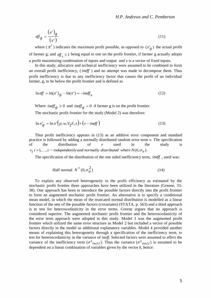
ggeff (11)

where ( ) indicates the maximum profit possible, as opposed to )( g the actual profit

of farmer g; and 1geff being equal to one on the profit frontier, if farmer g actually adopts

a profit maximizing combination of inputs and output and z is a vector of fixed inputs.

In this study, allocative and technical inefficiency were assumed to be combined to form

an overall profit inefficiency, ( ineff ) and no attempt was made to decompose them. Thus

profit inefficiency is due to any inefficiency factor that causes the profit of an individual

farmer, g, to be below the profit frontier and is defined as

gineffgeff )ln()ln(ln

(12)

Where 0gineff and 0gineff if farmer g is on the profit frontier.

The stochastic profit frontier for the study (Model 2) was therefore:

ineffvzVwpg ,1,,lnln

(13)

Thus profit inefficiency appears in (13) as an additive error component and standard

practice is followed by adding a normally distributed random error term v. The specification

of the distribution of v used in the study is

),0(~,,1 vNwhereddistributenormallyandtlyindependentiiv .

The specification of the distribution of the one sided inefficiency term, ineff , used was:

Half normal )2

,0( uN

(14)

To explain any observed heterogeneity in the profit efficiency as estimated by the

stochastic profit frontier three approaches have been utilized in the literature (Greene, 33-

38). One approach has been to introduce the possible factors directly into the profit frontier

to form an augmented stochastic profit frontier. An alternative is to specify a conditional

mean model, in which the mean of the truncated normal distribution is modelled as a linear

function of the sets of the possible factors (covariates) (STATA, p. 563) and a third approach

is to test for heteroscedasticity in the error terms. Greene argues that no approach is

considered superior. The augmented stochastic profit frontier and the heteroscedasticity of

the error term approach were adopted in this study. Model 3 was the augmented profit

frontier which utilized the same error structure as Model 2 but included a vector of possible

factors directly in the model as additional explanatory variables. Model 4 provided another

means of explaining this heterogeneity through a specification of the inefficiency term, to

test for heteroscedasticity in the variance of ineff. Selected factors were assumed to affect the

variance of the inefficiency term ( Thus the variance

is assumed to be

dependent on a linear combination of variables given by the vector k, hence:


6

),(~,,1 kNddistributetlyindependentiiineff

with truncation point at zero

and kineff

'2 (Model 4) (15)

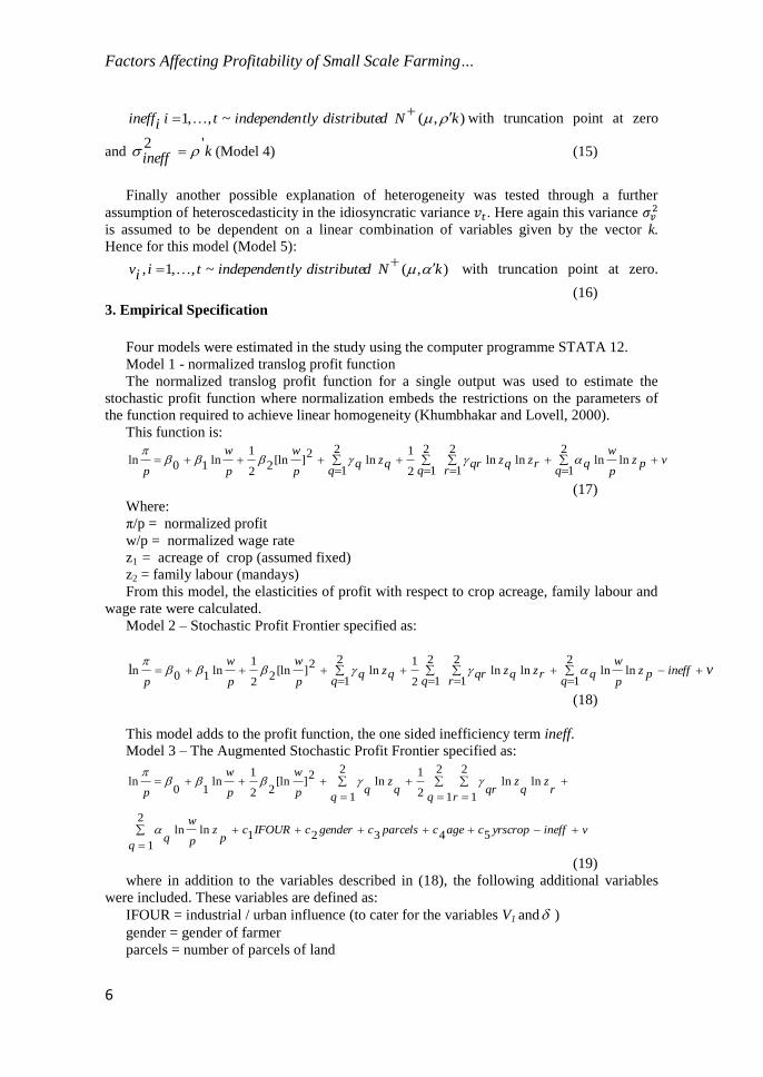
Finally another possible explanation of heterogeneity was tested through a further

assumption of heteroscedasticity in the idiosyncratic variance . Here again this variance

is assumed to be dependent on a linear combination of variables given by the vector k.

Hence for this model (Model 5):

),(~,,1, kNddistributetlyindependentiiv

with truncation point at zero.

(16)

3. Empirical Specification

Four models were estimated in the study using the computer programme STATA 12.

Model 1 - normalized translog profit function

The normalized translog profit function for a single output was used to estimate the

stochastic profit function where normalization embeds the restrictions on the parameters of

the function required to achieve linear homogeneity (Khumbhakar and Lovell, 2000).

This function is:

vpzp

w

qqrzqz

rqr

qqz

qq

p

w

p

w

p

lnln2

1lnln

2

1

2

12

1ln

2

1

2][ln2

2

1ln10ln

(17)

Where:

π/p = normalized profit

w/p = normalized wage rate

z1 = acreage of crop (assumed fixed)

z2 = family labour (mandays)

From this model, the elasticities of profit with respect to crop acreage, family labour and

wage rate were calculated.

Model 2 – Stochastic Profit Frontier specified as:

vineffpzp

w

qqrzqz

rqr

qqz

qq

p

w

p

w

p

lnln2

1lnln

2

1

2

12

1ln

2

1

2][ln2

2

1ln10nl

(18)

This model adds to the profit function, the one sided inefficiency term ineff.

Model 3 – The Augmented Stochastic Profit Frontier specified as:

vineffyrscropcagecparcelscgendercIFOURcp

zp

w

qq

rz

qz

rqr

qq

z

qqp

w

p

w

p

54321lnln2

1

lnln2

1

2

12

1ln

2

1

2][ln

22

1ln

10ln

(19)

where in addition to the variables described in (18), the following additional variables

were included. These variables are defined as:

IFOUR = industrial / urban influence (to cater for the variables V1 and )

gender = gender of farmer

parcels = number of parcels of land


7

yrscrop = years growing the crop

Model 4 was estimated to explain possible heteroscedasticity associated with the one-

sided inefficiency error term (ineff). The model had the same structure as (19) except for the

distribution of the error term, ineff, as noted earlier.

Model 5 was estimated to explain possible heteroscedasticity in the idiosyncratic error

term v. The model had the same structure as (19) except for the distribution of the

idiosyncratic error term v as noted earlier.

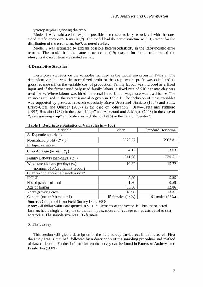
4. Descriptive Statistics

Descriptive statistics on the variables included in the model are given in Table 2. The

dependent variable was the normalized profit of the crop, where profit was calculated as

gross revenue minus the variable cost of production. Family labour was included as a fixed

input and if the farmer used only used family labour, a fixed rate of $10 per man-day was

used for w. Where labour was hired the actual hired labour wage rate was used for w. The

variables utilized in the vector k are also given in Table 1. The inclusion of these variables

was supported by previous research especially Bravo-Ureta and Pinhiero (1997) and Solis,

Bravo-Ureta and Quiroga (2009) in the case of “education”, Bravo-Ureta and Pinhiero

(1997) Hossain (1989) in the case of “age” and Adewumi and Adebayo (2008) in the case of

“years growing crop” and Kalirajan and Shand (1985) in the case of “gender”.

Table 1. Descriptive Statistics of Variables (n = 106)

Variable Mean Standard Deviation

A. Dependent variable

Normalized profit ( / p) 3375.37 7967.81

B. Input variables

Crop Acreage (acres) ( 1z ) 4.12 3.63

Family Labour (man-days) ( 2z ) 241.08 230.51

Wage rate (dollars per day) (w)

(nominal $10 /day family labour)

19.32 15.72

C. Farm and Farmer Characteristics*

IFOUR 5.89 5.35

No. of parcels of land 1.30 0.59

Age of farmer 53.36 12.86

Years growing crop 18.98 13.31

Gender (male=0 female =1) 15 females (14%) 91 males (86%)

Source: Computed from Field Survey Data, 2008

Note: All dollar values are quoted in $TT, * Elements of the vector k. Thus the selected

farmers had a single enterprise so that all inputs, costs and revenue can be attributed to that

enterprise. The sample size was 106 farmers.

5. The Survey

This section will give a description of the field survey carried out in this research. First

the study area is outlined, followed by a description of the sampling procedure and method

of data collection. Further information on the survey can be found in Patterson-Andrews and

Pemberton (2009).


8

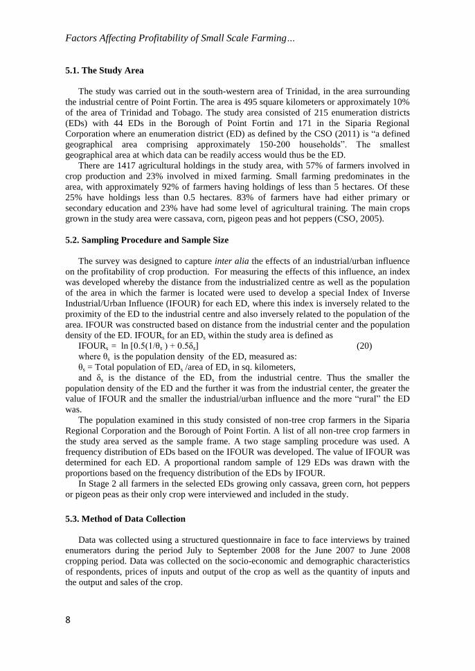
5.1. The Study Area

The study was carried out in the south-western area of Trinidad, in the area surrounding

the industrial centre of Point Fortin. The area is 495 square kilometers or approximately 10%

of the area of Trinidad and Tobago. The study area consisted of 215 enumeration districts

(EDs) with 44 EDs in the Borough of Point Fortin and 171 in the Siparia Regional

Corporation where an enumeration district (ED) as defined by the CSO (2011) is “a defined

geographical area comprising approximately 150-200 households”. The smallest

geographical area at which data can be readily access would thus be the ED.

There are 1417 agricultural holdings in the study area, with 57% of farmers involved in

crop production and 23% involved in mixed farming. Small farming predominates in the

area, with approximately 92% of farmers having holdings of less than 5 hectares. Of these

25% have holdings less than 0.5 hectares. 83% of farmers have had either primary or

secondary education and 23% have had some level of agricultural training. The main crops

grown in the study area were cassava, corn, pigeon peas and hot peppers (CSO, 2005).

5.2. Sampling Procedure and Sample Size

The survey was designed to capture inter alia the effects of an industrial/urban influence

on the profitability of crop production. For measuring the effects of this influence, an index

was developed whereby the distance from the industrialized centre as well as the population

of the area in which the farmer is located were used to develop a special Index of Inverse

Industrial/Urban Influence (IFOUR) for each ED, where this index is inversely related to the

proximity of the ED to the industrial centre and also inversely related to the population of the

area. IFOUR was constructed based on distance from the industrial center and the population

density of the ED. IFOURs for an EDs within the study area is defined as

IFOURs = ln [0.5(1/θs ) + 0.5δs] (20)

where θs is the population density of the ED, measured as:

θs = Total population of EDs /area of EDs in sq. kilometers,

and δs is the distance of the EDs from the industrial centre. Thus the smaller the

population density of the ED and the further it was from the industrial center, the greater the

value of IFOUR and the smaller the industrial/urban influence and the more “rural” the ED

was.

The population examined in this study consisted of non-tree crop farmers in the Siparia

Regional Corporation and the Borough of Point Fortin. A list of all non-tree crop farmers in

the study area served as the sample frame. A two stage sampling procedure was used. A

frequency distribution of EDs based on the IFOUR was developed. The value of IFOUR was

determined for each ED. A proportional random sample of 129 EDs was drawn with the

proportions based on the frequency distribution of the EDs by IFOUR.

In Stage 2 all farmers in the selected EDs growing only cassava, green corn, hot peppers

or pigeon peas as their only crop were interviewed and included in the study.

5.3. Method of Data Collection

Data was collected using a structured questionnaire in face to face interviews by trained

enumerators during the period July to September 2008 for the June 2007 to June 2008

cropping period. Data was collected on the socio-economic and demographic characteristics

of respondents, prices of inputs and output of the crop as well as the quantity of inputs and

the output and sales of the crop.


9

6. Results and Discussion

This section provides the descriptive statistics for the farmers and selected variables

included in the empirical specification of the stochastic profit frontier. In addition, it presents

the results of the estimation of the Stochastic Profit Frontier.

In Table 1, the mean farm size was found to be 4.12 acres with an average use of 241.08

man days of family labour and an average wage rate of $19.32 per day. Farms were in EDs

with an average IFOUR value 5.89. The mean number of years of formal schooling of

farmers was 8.81 years and they grew their crop on an average of 1.30 parcels of land. The

mean age of farmers was 53.36 years and they had been growing their crop for an average of

18.98 years. There were 15 females and 91 males in the sample. As seen in Table 2, the

mean acreage of the crop was 1.23 acres; with the average price of the crops as $4.60/lb with

pigeon peas being the crop fetching the highest price. The average profit per crop (farmer)

was $13841.09.

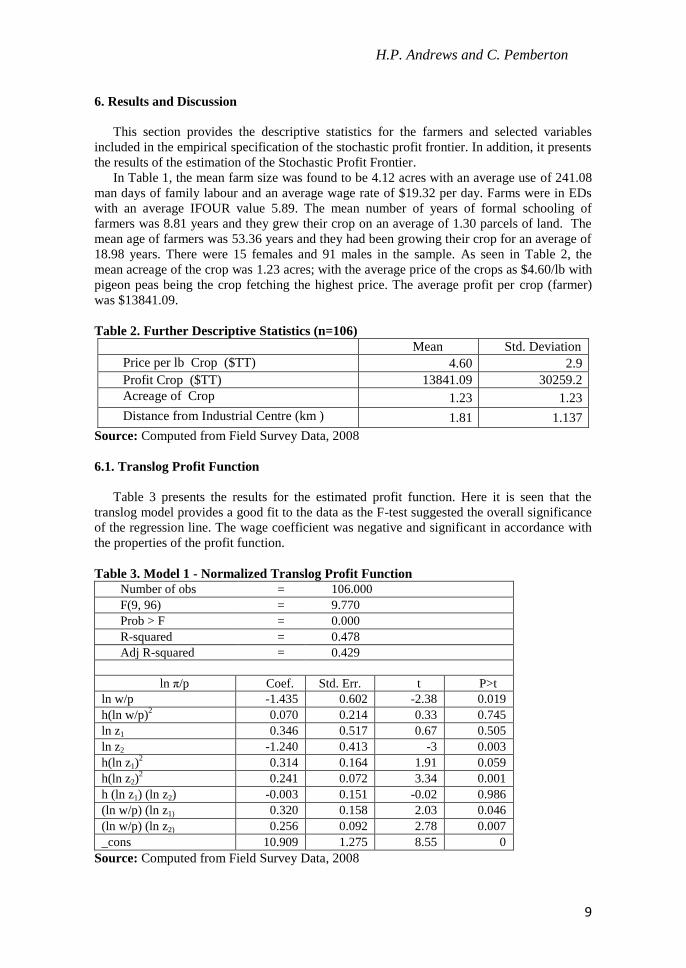
Table 2. Further Descriptive Statistics (n=106)

Mean Std. Deviation

Price per lb Crop ($TT) 4.60 2.9

Profit Crop ($TT) 13841.09 30259.2

Acreage of Crop 1.23 1.23

Distance from Industrial Centre (km ) 1.81 1.137


6.1. Translog Profit Function

Table 3 presents the results for the estimated profit function. Here it is seen that the

translog model provides a good fit to the data as the F-test suggested the overall significance

of the regression line. The wage coefficient was negative and significant in accordance with

the properties of the profit function.

Table 3. Model 1 - Normalized Translog Profit Function

Number of obs = 106.000

F(9, 96) = 9.770

Prob > F = 0.000

R-squared = 0.478

Adj R-squared = 0.429

ln π/p Coef. Std. Err. t P>t

ln w/p -1.435 0.602 -2.38 0.019

h(ln w/p)2 0.070 0.214 0.33 0.745

ln z1 0.346 0.517 0.67 0.505

ln z2 -1.240 0.413 -3 0.003

h(ln z1)2 0.314 0.164 1.91 0.059

h(ln z2)2 0.241 0.072 3.34 0.001

h (ln z1) (ln z2) -0.003 0.151 -0.02 0.986

(ln w/p) (ln z1) 0.320 0.158 2.03 0.046

(ln w/p) (ln z2) 0.256 0.092 2.78 0.007

_cons 10.909 1.275 8.55 0



10

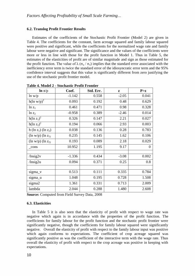
6.2. Translog Profit Frontier Results

Estimates of the coefficients of the Stochastic Profit Frontier (Model 2) are given in

Table 4. The coefficients for the constant, farm acreage squared and family labour squared

were positive and significant, while the coefficients for the normalized wage rate and family

labour were negative and significant. The significance and the values of the coefficients were

more or less in line with those for the profit function in Model 1. Thus in Table 5, the

estimates of the elasticities of profit are of similar magnitude and sign as those estimated for

the profit function. The value of λ (σu / σv) implies that the standard error associated with the

inefficiency error term is twice the standard error of the idiosyncratic error term and the 95%

confidence interval suggests that this value is significantly different from zero justifying the

use of the stochastic profit frontier model.

Table 4. Model 2 - Stochastic Profit Frontier

ln π/p Coef. Std. Err. z P>z

ln w/p -1.142 0.558 -2.05 0.041

h(ln w/p)2 0.093 0.192 0.48 0.629

ln z1 0.461 0.471 0.98 0.328

ln z2 -0.958 0.389 -2.46 0.014

h(ln z1)2 0.326 0.147 2.21 0.027

h(ln z2)2 0.194 0.066 2.93 0.003

h (ln z1) (ln z2) 0.038 0.136 0.28 0.783

(ln w/p) (ln z1) 0.235 0.145 1.62 0.106

(ln w/p) (ln z2) 0.193 0.089 2.18 0.029

_cons 10.952 1.195 9.17 0

/lnsig2v -1.336 0.434 -3.08 0.002

/lnsig2u 0.094 0.371 0.25 0.8

sigma_v 0.513 0.111 0.335 0.784

sigma_u 1.048 0.195 0.728 1.508

sigma2 1.361 0.331 0.713 2.009

lambda 2.044 0.288 1.480 2.608


6.3. Elasticities

In Table 5 it is also seen that the elasticity of profit with respect to wage rate was

negative which again is in accordance with the properties of the profit function. The

coefficients for family labour for the profit function and the stochastic profit frontier were

significantly negative, though the coefficients for family labour squared were significantly

negative. Overall the elasticity of profit with respect to the family labour input was positive

which again conforms to expectations. The coefficient of crop acreage squared was

significantly positive as was the coefficient of the interactive term with the wage rate. Thus

overall the elasticity of profit with respect to the crop acreage was positive in keeping with

expectations.


11

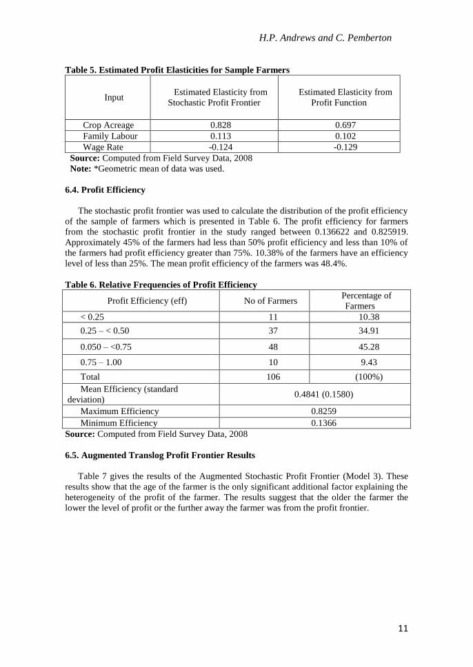
Table 5. Estimated Profit Elasticities for Sample Farmers

Input Estimated Elasticity from

Stochastic Profit Frontier

Estimated Elasticity from

Profit Function

Crop Acreage 0.828 0.697

Family Labour 0.113 0.102

Wage Rate -0.124 -0.129


Note: *Geometric mean of data was used.

6.4. Profit Efficiency

The stochastic profit frontier was used to calculate the distribution of the profit efficiency

of the sample of farmers which is presented in Table 6. The profit efficiency for farmers

from the stochastic profit frontier in the study ranged between 0.136622 and 0.825919.

Approximately 45% of the farmers had less than 50% profit efficiency and less than 10% of

the farmers had profit efficiency greater than 75%. 10.38% of the farmers have an efficiency

level of less than 25%. The mean profit efficiency of the farmers was 48.4%.

Table 6. Relative Frequencies of Profit Efficiency

Profit Efficiency (eff) No of Farmers Percentage of

Farmers

< 0.25 11 10.38

0.25 – < 0.50 37 34.91

0.050 – <0.75 48 45.28

0.75 – 1.00 10 9.43

Total 106 (100%)

Mean Efficiency (standard

deviation) 0.4841 (0.1580)

Maximum Efficiency 0.8259

Minimum Efficiency 0.1366


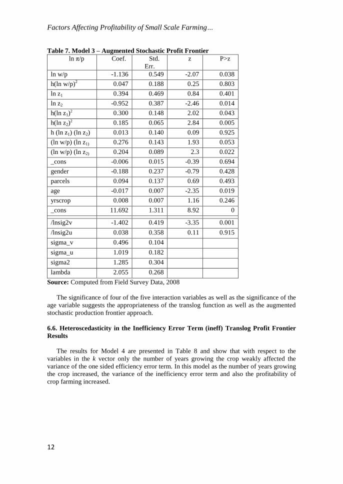
6.5. Augmented Translog Profit Frontier Results

Table 7 gives the results of the Augmented Stochastic Profit Frontier (Model 3). These

results show that the age of the farmer is the only significant additional factor explaining the

heterogeneity of the profit of the farmer. The results suggest that the older the farmer the

lower the level of profit or the further away the farmer was from the profit frontier.


12

Table 7. Model 3 – Augmented Stochastic Profit Frontier

ln π/p Coef. Std.

Err.

z P>z

ln w/p -1.136 0.549 -2.07 0.038

h(ln w/p)2 0.047 0.188 0.25 0.803

ln z1 0.394 0.469 0.84 0.401

ln z2 -0.952 0.387 -2.46 0.014

h(ln z1)2 0.300 0.148 2.02 0.043

h(ln z2)2 0.185 0.065 2.84 0.005

h (ln z1) (ln z2) 0.013 0.140 0.09 0.925

(ln w/p) (ln z1) 0.276 0.143 1.93 0.053

(ln w/p) (ln z2) 0.204 0.089 2.3 0.022

_cons -0.006 0.015 -0.39 0.694

gender -0.188 0.237 -0.79 0.428

parcels 0.094 0.137 0.69 0.493

age -0.017 0.007 -2.35 0.019

yrscrop 0.008 0.007 1.16 0.246

_cons 11.692 1.311 8.92 0

/lnsig2v -1.402 0.419 -3.35 0.001

/lnsig2u 0.038 0.358 0.11 0.915

sigma_v 0.496 0.104

sigma_u 1.019 0.182

sigma2 1.285 0.304

lambda 2.055 0.268


The significance of four of the five interaction variables as well as the significance of the

age variable suggests the appropriateness of the translog function as well as the augmented

stochastic production frontier approach.

6.6. Heteroscedasticity in the Inefficiency Error Term (ineff) Translog Profit Frontier

Results

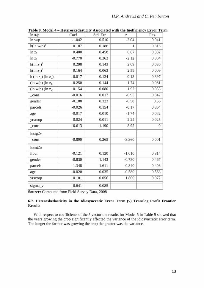
The results for Model 4 are presented in Table 8 and show that with respect to the

variables in the k vector only the number of years growing the crop weakly affected the

variance of the one sided efficiency error term. In this model as the number of years growing

the crop increased, the variance of the inefficiency error term and also the profitability of

crop farming increased.


13

Table 8. Model 4 – Heteroskedasticity Associated with the Inefficiency Error Term


ln w/p -1.042 0.510 -2.04 0.041

h(ln w/p)2 0.187 0.186 1 0.315

ln z1 0.400 0.458 0.87 0.382

ln z2 -0.770 0.363 -2.12 0.034

h(ln z1)2 0.298 0.143 2.09 0.036

h(ln z2)2 0.164 0.063 2.59 0.009

h (ln z1) (ln z2) -0.017 0.134 -0.13 0.897

(ln w/p) (ln z1) 0.250 0.144 1.74 0.081

(ln w/p) (ln z2) 0.154 0.080 1.92 0.055

_cons -0.016 0.017 -0.95 0.342

gender -0.188 0.323 -0.58 0.56

parcels -0.026 0.154 -0.17 0.864

age -0.017 0.010 -1.74 0.082

yrscrop 0.024 0.011 2.24 0.025

_cons 10.613 1.190 8.92 0

lnsig2v

_cons -0.890 0.265 -3.360 0.001

lnsig2u

ifour -0.121 0.120 -1.010 0.314

gender -0.830 1.143 -0.730 0.467

parcels -1.348 1.611 -0.840 0.403

age -0.020 0.035 -0.580 0.563

yrscrop 0.101 0.056 1.800 0.072

sigma_v 0.641 0.085


6.7. Heteroskedasticity in the Idiosyncratic Error Term (v) Translog Profit Frontier

Results

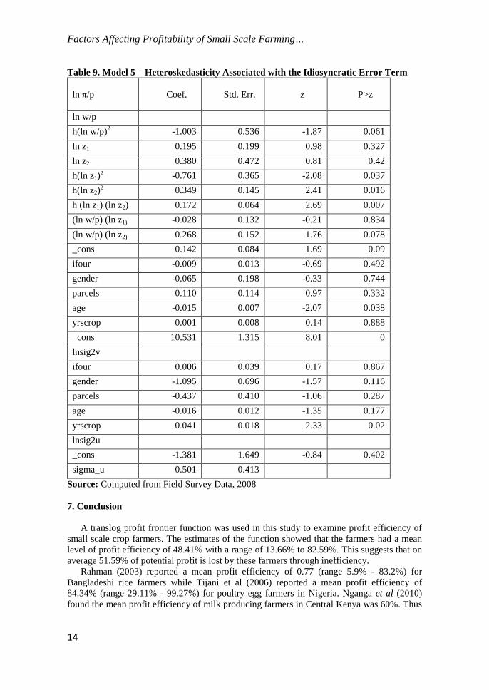
With respect to coefficients of the k vector the results for Model 5 in Table 9 showed that

the years growing the crop significantly affected the variance of the idiosyncratic error term.

The longer the farmer was growing the crop the greater was the variance.


14

Table 9. Model 5 – Heteroskedasticity Associated with the Idiosyncratic Error Term


ln w/p

h(ln w/p)2 -1.003 0.536 -1.87 0.061

ln z1 0.195 0.199 0.98 0.327

ln z2 0.380 0.472 0.81 0.42

h(ln z1)2 -0.761 0.365 -2.08 0.037

h(ln z2)2 0.349 0.145 2.41 0.016

h (ln z1) (ln z2) 0.172 0.064 2.69 0.007

(ln w/p) (ln z1) -0.028 0.132 -0.21 0.834

(ln w/p) (ln z2) 0.268 0.152 1.76 0.078

_cons 0.142 0.084 1.69 0.09

ifour -0.009 0.013 -0.69 0.492

gender -0.065 0.198 -0.33 0.744

parcels 0.110 0.114 0.97 0.332

age -0.015 0.007 -2.07 0.038

yrscrop 0.001 0.008 0.14 0.888

_cons 10.531 1.315 8.01 0

lnsig2v

ifour 0.006 0.039 0.17 0.867

gender -1.095 0.696 -1.57 0.116

parcels -0.437 0.410 -1.06 0.287

age -0.016 0.012 -1.35 0.177

yrscrop 0.041 0.018 2.33 0.02

lnsig2u

_cons -1.381 1.649 -0.84 0.402

sigma_u 0.501 0.413


7. Conclusion

A translog profit frontier function was used in this study to examine profit efficiency of

small scale crop farmers. The estimates of the function showed that the farmers had a mean

level of profit efficiency of 48.41% with a range of 13.66% to 82.59%. This suggests that on

average 51.59% of potential profit is lost by these farmers through inefficiency.

Rahman (2003) reported a mean profit efficiency of 0.77 (range 5.9% - 83.2%) for

Bangladeshi rice farmers while Tijani et al (2006) reported a mean profit efficiency of

84.34% (range 29.11% - 99.27%) for poultry egg farmers in Nigeria. Nganga et al (2010)

found the mean profit efficiency of milk producing farmers in Central Kenya was 60%. Thus


15

based on previous research, the profit efficiency of the farmers in this study was very low by

international comparison.

The variable formulated to measure the industrial/urban influence, IFOUR, did not

significantly affect the profitability. These results may imply that the positive effects of

industrial/urban influence were counteracted by the additional marketing cost to sell products

at the industrial/urban centre.

Proposition 2 was supported in the study by both the coefficient of the wage rate as well

as the elasticity of profit with respect to the wage rate being negative. This indicates the

importance of wage rates to the profitability of small scale crop production in the study.

With respect to Proposition 3, two socio-economic variables were significant in affecting

the profitability of crop farming.

The age of the farmer significantly affected profitability with increasing age reducing

profitability. Since the average age of farmers in the study was 53.36 years, policy measures

should be implemented geared at increasing the level of youths entering the agricultural field

and specifically crop production in Trinidad and Tobago.

The years growing the crop positively influenced the variance of both the one-sided error

term (ineff) as well as the idiosyncratic error term (v) and also the profitability of crop

farming.

The results of this study suggests that education and skill acquisition programmes in

agriculture should be organized in the study area, especially for young people to become

involved in agriculture, to enable them to maximize the use modern technology to increase

profit levels in crop farming in the study area.

8. References

Ali, F., Parikh, A., & Shah, M. (1994). Measurement of Profit Efficiency using Behavioral

and Stochastic Frontier Approaches. Applied Economics, 26(2), 181-188.

Atlantic LNG. (2014). About Us, Retrieved from http://www.atlanticlng.com/about-us

Aung, N. M. (2011). Agricultural Efficiency of Rice Farmers in Myanmar: A Case Study in

Selected Areas: No 306, IDE Discussion Papers No. 306. 2011.9. Institute of Developing

Economies, Japan External Trade Organization (JETRO).

Boserup, E. (1965). The Conditions of Agricultural Growth: The Economics of Agrarian

Change under Population Pressure. London: Earthscan Publications Ltd.

Camara Y., S. J. M. a. C. E. Comparing The Profitability Of Cassava-Based Production

Systems in Three West African Countries: Cote d’Ivoire, Ghana and Nigeria. Staff Paper

Series: Staff Papers 11593, 2001-03 Michigan State University, Department of

Agricultural, Food and Resource Economics, Retrieved from http://purl.umn.edu/11593

Central Statistical Office of Trinidad and Tobago (CSO). (2005). 2004 Agricultural Census

Report for Trinidad and Tobago. The Republic of Trinidad and Tobago: CSO. Retrieved

from http://cso.planning.gov.tt/content/agricultural-statistics-report

Central Statistical Office of Trinidad and Tobago (CSO). (2011). Trinidad and Tobago 2011

Population and Housing Census - Demographic Report. The Republic of Trinidad and

Tobago: CSO. Retrieved from

https://guardian.co.tt/sites/default/files/story/2011_DemographicReport.pdf

Chiang, A. (1984). Fundamental Methods of Mathematical Economics. New York: Mc

Graw-Hill.

Coelli, T. J., Rao, D.S.P., O'Donnell, C.J., & Battese, G.E. An Introduction to Efficiency and

Productivity Analysis (2 ed.). New York: Springer Science + Business Media, LLC.

Greene, W. (2007). LIMDEP Version 9: Econometric Modeling Guide Econometric Software

Inc. Plainview, NY: Econometric Software Inc.

http://www.atlanticlng.com/about-us

http://purl.umn.edu/11593


16

Grigorios, L., Moss, C. B., Breneman, V., & Nehring, R. (2006). Urban Sprawl and

Farmland Prices American. American Journal of Agricultural Economics, 88(4), 915-

929.

Hayami, Y. (1969). Sources of Agricultural Productivity Gap among Selected Countries.

American Journal of Agricultural Economics, 51(3), 564-575.

Hazell, P. (2004). Commentary: Last Chance for the Small Farm? IFPRI Newsletter IFPRI

Forum 2004 Retrieved from

http://www.ifpri.org/pubs/newsletters/IFPRIForum/200410/if08small .htm

Henneberry, S. R., M.E. Khan & K. Piewthongngam. (2000). An Analysis of Industrial-

Agricultural Interactions: A Case Study in Pakistan. Agricultural Economics, 22(1), 17-

27.

Hyuha, T. S., B. Bashaasha, E. Nkonya & D. Kraybill (2007). Analysis of Profit inefficiency

in Rice Production in Eastern and Northern Uganda. African Crop Science Journal,

15(4), 243-253.

Kumbhakar, S. C., & Lovell, C. A. K. (2000). Stochastic Frontier Analysis. Cambridge:

Cambridge University Press.

Lewis, W. A. (1975). Economic Development with Unlimited Supplies of Labour. The

Manchester School, May 1954. In A. N. Agarwala & S. P. Singh (Eds.), The Economics

of Underdevelopment. New Delhi: Oxford University Press.

Liverpool-Tasie, L. S., Kuku, O., & Ajibola, A. (2011). International Food Policy Research

Institute, Nigeria Strategy Support Program (NSSP): NSSP Working Paper No. 21

October 2011. Retrieved from

http://www.ifpri.org/sites/default/files/publications/nsspwp21.pdf

Ministry of Agriculture Land and Marine Resources. (2008). Strategies for Increasing

Agricultural Production for Food and Nutrition Security in Trinidad and Tobago.

Republic of Trinidad and Tobago.

Mitchell, D. (2008). A Note on Rising Food Prices. World Bank Policy Research Working

Paper Series, No. 4682. New York: World Bank.

Molnar, J., Hoban, T., Parish, J. D., & Futreal, M. (1997). Industrialization of Agriculture:

Trends, Spatial Patterns, and Implications for Field-level Application by the Natural

Resource Conservation Service. Social Sciences Institute Technical Report Release 5.1.

U.S. Department of Agriculture (USDA), Natural Resources Conservation Service, Social

Science Institute. Greensboro, NC.

Nganga, S. K., Kungu, J., de Ridder, N., & Herrero, M. (2010). Profit efficiency among

Kenyan smallholders milk producers: A case study of Meru-South district, Kenya.

African Journal of Agricultural Research, 5(4), 332-337.

NRI (2002) Natural Resources Institute UK: Chatham. (2002). Smallholders in Export

Horticulture: a Guide to Best Practices: The University of Greenwich 2002.

Onu, J. I., & Edon, A. (2009). Comparative Economic Analysis of Improved and Local

Cassava Varieties in Selected Local Government Areas of Taraba State, Nigeria. Journal

Soc. Sci., 19(3), 213-217.

Patterson-Andrews, H. & Pemberton, C. (2009). Factors Affecting the Relative

Competitiveness of Cassava Production in Southwestern Trinidad. Tropical Agriculture

(Trinidad), 86(4), 159-168.

Rahman, S. (2003). Profit Efficiency Among Bangladeshi Rice Farmers. Paper presented at

the International Association of Agricultural Economists 2003 Annual Meeting, August

6-22, 2003, Durban, South Africa.

Republic of Trinidad and Tobago, Ministry of Agriculture, Land and Marine Resources.

(2008). Strategies for Increasing Agricultural Production for Food and Nutrition Security

in Trinidad and Tobago.

http://www.ifpri.org/pubs/newsletters/IFPRIForum/200410/if08small%20.htm

http://www.ifpri.org/sites/default/files/publications/nsspwp21.pdf


17

Sexton, R. J. (2000). Industrialization and Consolidation in the US Food Sector: Implications

for Competition and Welfare. Amer. J. Agr. Econ. , 82(5), 1087-1107.

Sonka, S. (2003). Forces Driving Industrialization of Agriculture: Implications for the Grain

Industry in the United States. Paper presented at the Product Differentiation and Market

Segmentation in Grains and Oilseeds: Implications for Industry in Transition sponsored

by Economic Research Service, USDA and The Farm Foundation, Washington, DC

January 27-28, 2003.

Timothy, A. T., & Adeoti, A. I. (2006). Gender Inequalities and Economic Efficiency: New

Evidence from Cassava-based Farm Holdings in Rural South-Western Nigeria. African

Development Review, 18(3), 428-443.

Todaro, M. P. (2000). Economic Development (7 ed.). New York: Addison-Wesley Longman

Inc., p. 291.

United Nations Industrial Development Organization (UNIDO). (2009). Industrial

Development Report 2009: Breaking In and Moving Up: New Industrial Challenges for

the Bottom Billion and the Middle Income Countries. from 2009 United Nations

Industrial Development Organization (UNIDO)


18

Documents

FACTORS AFFECTING PROFITABILITY OF SMALL SCALE · PDF file · 2018-01-12Factors Affecting Profitability of Small Scale Farming 2 tendency of firms to cluster, either because of the