Embed Size (px)
Citation preview

6
DESIGN,FABRICATION,INSTALLATION,AND PERFORMANCEOF THE ACCELERATORSTRUCTURE
R. P. Borghi, A. L. Eldredge, R. H. Helm, A. V. Lisin,G. A. Loew, Editor and R. B. Neal
The purpose of this chapter is to describe the heart of the accelerator, theperiodic waveguide structure which is used to accelerate the electrons. Asdiscussed in Chapter 3, the design of the two-mile machine at SLAC is alogical extension of accelerator developments at Stanford University since1947.1'2 By the time the SLAC project was authorized in 1961, Stanfordworkers had reached a high degree of confidence and familiarity with thedesign and fabrication of disk-loaded waveguides. Although several othertypes of periodic structures were investigated as discussed later in this chapter,the disk-loaded waveguide was selected as the best overall structure meetingmost design and fabrication criteria.
This chapter is divided into four parts. The first is concerned with a dis-cussion of accelerator theory and selection of characteristic parameters. It isfollowed by a description of the empirical design used to achieve the selectedparameters. The third part is a description of fabrication techniques, assem-bly, and installation. Finally, a summary of performance is given.
6-1 Theory and selection of characteristic parameters
Choice of operating frequency (RBN)
Because almost all the basic accelerator parameters have frequency depend-ence, it was first essential to compare the advantages and disadvantages ofthe various frequency bands and to choose an operating frequency. However,it was not possible to make the choice of frequency by purely analyticalmethods; the final selection required engineering judgment and reference toprevious experience.
95

96 G. A. Loew et a/.
The laws of frequency dependence of the principal parameters involvedin the design of a linac are listed in Table 6-1. To simplify the comparison,this table assumes direct scaling of the modular dimensions of the acceleratingstructure. For a specific accelerator some compromises must be made whichmodify Table 6-1 in certain details but do not alter its general implications.
The energy of electrons from a linear accelerator with negligible beamloading is given by
rQY'2 (6-1)
where PT is the total input RF power, L is the total length, r0 is the shuntimpedance per unit length, and K is a constant of which the value dependsupon the net RF attenuation in each independently fed accelerator section.
Table 6-1 Frequency dependence of principal machine parameters
Parameter
Shunt impedance per unit length (r)
RF loss factor (Q)
Filling time (/F)Total RF peak power
RF feed interval (/)
No. of RF feedsRF peak power per feed
RF energy stored in accelerator
Beam loading (—dV/di)
Peak beam current at maximumconversion efficiency
Diameter of beam aperture
Maximum RF power available fromsingle source
Maximum permissible electric fieldstrength
Relative frequency and dimen-sional tolerances
Absolute wavelength and dimen-sional tolerances
Power dissipation capability ofaccelerator structure
Frequencydependence
fl/2
f-1/2
f-3/2
f-1/2
f-3/2
f3/2
f~2
f~2
fl/2
f-1/2
f'1
f~2
fl/2
fl/2
f-1/2
f-1
Frequencypreference
High
X
X
X
X
X
X
X
Low
X
X
X
X
X
X
X
X
X
Notes
a
a
a, b
a, b, c
a, b
a, b, da, b, c
a, b, c
a, b, d
a, b, c, f
a
e
g
a, b
a,b
a, b, d
Notes:a. For direct scaling of modular dimensions of accelerator structure.b. For same RF attenuation in accelerator section between feeds.c. For fixed electron energy and total length.d. For fixed total length.e. When limited by cathode emission.f. When limited by beam loading.g. Approximate; empirical.

Design, fabrication, installation, and performance 97
Since r0 varies as/1/2, the RF power required to produce a given final energyin a fixed length is proportional to/~1/2. Thus, considerations of powereconomy indicated that the operating frequency should be as high as possible.Other advantages of the higher frequencies are the reduced filling time, whichvaries as/~3/2, and reduced energy storage, which varies as/~2. A shorterfilling time is advantageous since electrons can be accelerated during a largerfraction of the available RF pulse length. The use of the higher frequenciesalso results in greater maximum field strength (as limited by breakdown) andlarger relative frequency and dimensional tolerances.
From Table 6-1 it can be seen that the maximum frequency which can beused is limited by the diameter of the aperture available for the beam and bythe reduced, beam current capability. Another factor against the use of veryhigh frequencies is the increased number of power sources and feeds required.The increased cost of additional RF systems, modulators, and controls, andthe increased operational difficulties which are encountered tend to offset theadvantages arising from decreased power consumption at high frequencies.
An important consideration not taken into account in Table 6-1 was thedegree of conservatism involved in the choice of frequency band. Althoughlinear electron accelerators had been constructed and operated at L-, S-, andX-bands, the largest amount of experience was available at S-band. In fact,to this date all accelerators of this type having energies above 100 MeV haveoperated at S-band.
To illustrate the scaling laws given in Table 6-1 more specifically, designdata for a 20-GeV accelerator 10,000 ft long are given in Table 6-2. Threecases are tabulated corresponding to operating at L-, S-, and X-bands. Thespecific values in Table 6-2 were based on relations and criteria which aredeveloped later in this section. While each item in Table 6-2 need not bediscussed individually, it may be worthwhile to emphasize the followingpoints:
1. An important aspect of the design of the two-mile accelerator was thepossibility of increasing the beam energy at some future date from itspresent maximum of 20 GeV to a higher level between 20 and 40 GeV.For reasons of economy and to avoid prolonged machine shutdown, itappeared desirable to make such an energy expansion possible by increas-ing the RF power rather than the accelerator length. According to Table6-2, the L-band structure with a fixed length of 10,000 ft could not beexpanded above about 38.4 GeV without experiencing breakdown diffi-culties.
2. The average RF power requirements were in the ratio 4.1/1.0/0.4 for theL-, S-, and X-band machines, respectively.
3. The maximum peak beam currents and beam powers were in the ratiosof 1.7/1.0/0.6 for the L-, S-, and X-band machines, respectively.
4. The aperture available for the beam in the X-band machine (0.255 in.)would have been small enough to cause great concern about beam trans-mission and accelerator alignment.

98 G. A. Loew et al.
Table 6-2 Design parameters of 20-GeV accelerator at three frequencies"
Parameter(L-Band)
1000 MHz
Frequency
(S-Band)3000 MHz
(X-Band)9000 MHz
Shunt impedance r (megohms/meter) 31 53 92
RF.Ioss factor (0) 2.25 x 10⁴ 1.3 x 10⁴ 0.75 x 10⁴
Filling time tF (p-sec) 4.31 0.83 0.16Total RF peak power (MW) 9216 5320 3072RF feed interval (ft) 52 10 1.92No. of RF feeds 185 960 4988RF peak power (MW) per feed 50 5.54 0.62RF energy (J) stored in accelerator 21,348 2372 264RF energy (J) required for 1.67-
jiisec electron beam pulselength 55,112 13,300 5,620
Total average RF power (MW) at360 pulses/sec 19.84 4.80 2.04
Beam loading (-dV/di) (GeV/A) 20.5 35.5 61.5Peak beam current (mA) at maxi-
mum conversion efficiency 544.2 314.2 181.4Minimum diameter (in.) of beam
aperture 2.292 0.764 0.255Maximum RF peak power (MW)
from single source6 216 24 2.7Maximum permissible electric
field strength6 (kV/cm) 133 230 398Maximum expanded beam
energy" (GeV) 38.4 66.5 115.0Relative frequency and dimen-
sional tolerances6 1.11x10~5 1.93X1Q-5 3.34 x10~ 5
Absolute frequency and dimen- 11 kHz 58kHz 301 kHzsional tolerances6 0.11 mils 0.06 mils 0.04 mils
Average power dissipated perunit area of accelerator surface/
(W/cm2) 0.59 0.43 0.53Average temperature difference
(°C) across accelerator wall9 0.42 0.10 0.04
• Assumptions: 277/3 mode in constant-gradient structure; T= 0.57 Np (RF attenuation); L = 10,000 ft(94.8% effective); 10% power loss in waveguides; 10% beam loading; direct scaling of modular dimensions.6 Based on 24 MW available at S-band, values for other frequencies based on scaling as/"2.c Based on maximum gradient obtained to date at S-band; values for other frequencies based on scaling
as/1/2.d As limited by maximum permissible field strength.e For 1% loss in beam energy.f Based on 360 pulses/sec and 1.6-/tsec electron beam pulse length.« Based on copper wall 3, 1, and i cm thick at L-, S-, and X-bands, respectively.

Design, fabrication, installation, and performance 99
5. The X-band accelerator ranked highest in terms of maximum expandedenergy capability, but the higher energies required X-band sources ofhigher peak power than were available. For example, operation at 40 GeVwould have required 4988 sources each producing 2.5 MW of peak RFpower.
6. Expansion of the L-band accelerator to 40 GeV would have required thateach of the 185 feed points be supplied with 200 MW of peak power.Such power would have been much higher than the power output obtain-able from a single L-band source and would have required paralleloperation of several sources at each feed.
7. Expansion of the S-band machine to 40 GeV would have required 22.2 MWat each of the 960 feed points. Power outputs above this level had alreadybeen obtained quite easily from single S-band sources.
8. The relative frequency and dimensional tolerances favored the use of thehigher frequencies. Relative dimensional tolerances are probably moresignificant than absolute tolerances, since the former are a better measureof the difficulties involved in critical machining operations.
9. The average power dissipated per unit area of accelerator surface was notsignificantly different in the three designs because the increased wall areaat low frequency tended to compensate for the higher power requiredand vice versa. However, the average temperature difference across theaccelerator wall, which is a measure of the degree of detuning of thestructure, was highest at L-band and lowest at X-band.
It would have been possible to compare accelerator designs at the variousfrequencies in further detail. The designs that were chosen for illustrativepurposes were based upon direct scaling of the modular dimensions of exist-ing S-band accelerator structures. An improved design at a particular fre-quency from the standpoint of overall economy or performance may havebeen obtained by deviating from the scaling laws that were used. For example,the L-band design might have been improved by decreasing the feed intervaland using a larger number of sources, and by increasing the RF and beampulse lengths while decreasing the pulse repetition rate. However, this wouldnot have affected the total peak power requirement or the maximum, fieldstrength capability. Similar alterations might have been made at S- and X-bands to improve certain characteristics of these designs. However, suchchanges would not have modified appreciably the general conclusion that wasreached, namely that S-band was the optimum choice for the two-mileaccelerator for reasons implicit in the scaling laws of Table 6-1 and theillustrative examples of Table 6-2.
Product of RF power and accelerator length (RBN)
The energy of electrons from a linear accelerator with negligible beam loadingwas given by Eq. (6-1). To estimate the power-length product of the two-mileaccelerator, the values of two important parameters discussed later in this
100 G. A. Loew et al.
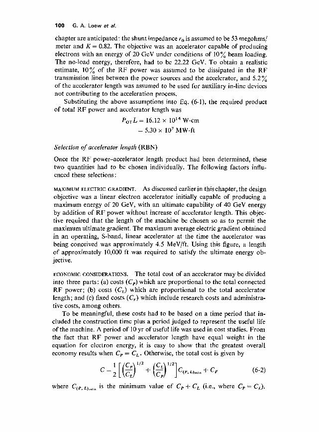
chapter are anticipated : the shunt impedance r0 is assumed to be 53 megohms/meter and K = 0.82. The objective was an accelerator capable of producingelectrons with an energy of 20 GeV under conditions of 10% beam loading.The no-load energy, therefore, had to be 22.22 GeV. To obtain a realisticestimate, 10% of the RF power was assumed to be dissipated in the RFtransmission lines between the power sources and the accelerator, and 5.2 %of the accelerator length was assumed to be used for auxiliary in-line devicesnot contributing to the acceleration process.
Substituting the above assumptions into Eq. (6-1), the required productof total RF power and accelerator length was
POTL= 16.12 x 10¹⁴W-cm
= 5.30 x 10⁷ MW-ft
Selection of accelerator length (RBN)
Once the RF power-accelerator length product had been determined, thesetwo quantities had to be chosen individually. The following factors influ-enced these selections:
MAXIMUM ELECTRIC GRADIENT. As discussed earlier in this chapter, the designobjective was a linear electron accelerator initially capable of producing amaximum energy of 20 GeV, with an ultimate capability of 40 GeV energyby addition of RF power without increase of accelerator length. This objec-tive required that the length of the machine be chosen so as to permit themaximum ultimate gradient. The maximum average electric gradient obtainedin an operating, S-band, linear accelerator at the time the accelerator wasbeing conceived was approximately 4.5 MeV/ft. Using this figure, a lengthof approximately 10,000 ft was required to satisfy the ultimate energy ob-jective.
ECONOMIC CONSIDERATIONS. The total cost of an accelerator may be dividedinto three parts: (a) costs (CP) which are proportional to the total connectedRF power; (b) costs (CL) which are proportional to the total acceleratorlength ; and (c) fixed costs (Cf ) which include research costs and administra-tive costs, among others.
To be meaningful, these costs had to be based on a time period that in-cluded the construction time plus a period judged to represent the useful lifeof the machine. A period of 10 yr of useful life was used in cost studies. Fromthe fact that RF power and accelerator length have equal weight in theequation for electron energy, it is easy to show that the greatest overalleconomy results when CP = CL . Otherwise, the total cost is given by
where C(P L)min is the minimum value of CP + CL (i.e., where CP = CL).

Design, fabrication, installation, and performance 101
These cost studies showed that an accelerator length of 10,000 ft was veryclose to the optimum value to minimize the total project costs over theinitially projected 6-yr construction period and a 10-yr period of operation.
LAND AVAILABLITY. There were several potential sites available on Stanfordland which seemed suitable for the accelerator project location. An accelera-tor length of 10,000 ft (plus another 2500 ft, approximately, for researchfacilities) was possible at most of these sites, but no greater length was avail-able without high land acquisition costs.
Thus the choice of an accelerator length of 10,000 ft satisfied the severalconditions discussed above: namely, it permitted operation at the ultimate,expanded energy gradient; it was near optimum from the standpoint of over-all economy; and such space was available on Stanford property. Using thepower-length product determined in an earlier section led to an initial totalconnected RF power requirement of
POT = 5.32 x 10³ MW
It should be emphasized that this value of POT was based upon a particularchoice of operating mode (2rc/3) and a particular attenuation parameter(T = 0.57). Their selection is discussed later in this section. The value of POT
would vary slightly if another mode or another value of T had been used.
Selection of number of RF power sources and feed interval (RBN)
It was established in the previous section that a total RF peak power of 5320MW had to be supplied by the power sources in order to achieve an electronenergy of 20 GeV with 10% beam loading in a 10,000-ft accelerator. The nextlogical design decisions were the determination of the number of individualRF power sources and the spacing of the RF feeds along the acceleratorlength.
In general, it is more economical to obtain a large amount of microwaveenergy from a small number of high-power sources than from a large numberof low-power sources. The basic reason for this fact is that the cost of a powersource depends more strongly on the number and kind of operations involvedin its fabrication and processing than upon its physical size and output rating.The cost of employment of the power sources in the accelerator system interms of auxiliary equipment, such as instrumentation, controls, and wave-guide equipment, also decreases as the total number of individual sources isreduced. Based upon laboratory and commercial experience with high-powerklystron amplifiers, it seemed reasonable to expect that S-band tubes couldbe constructed to have an average life of 2000 hours or more while producing24 MW of peak RF power and 22 kW of average RF power. Much higher,peak power levels from single S-band tubes did not appear to be readilyobtainable at the time. An electron beam energy of 20 GeV could be obtainedby requiring 24 MW of peak output per klystron. For a total RF power of

102 G. A. Loew et al.
5320 MW, 240 klystrons producing 24 MW each were needed. For operationat the Stage II level of 40 GeV, 960 tubes producing 24 MW each would berequired.
The selection of the feed spacing along the accelerator length will now bediscussed. The limiting cases of feed spacing were (a) a single feed for theentire accelerator, and (b) individual feeds for each of the approximately80,000 individual accelerator cavities. The first extreme was obviously un-feasible because the full RF power could not be transmitted through theaccelerator structure. The second extreme would have been prohibitivelyexpensive because of the multiplicity of waveguides and other microwavecomponents and the necessary controls and instrumentation. As describedin a later section, there is an optimum, or at least a preferred value, of thenet RF attenuation between feed points. The choice of attenuation parameteris a compromise among many factors. The attenuation parameter can beadjusted to the desired value by properly choosing the diameter of theaperture in the disk-loaded structure and the length of the acceleratorsection—increasing the aperture size increases the group velocity and de-creases the attenuation per unit length. Thus a given attenuation parametercan be obtained by either a short accelerator section of high unit attenuation(small aperture), or by a long section of low unit attenuation (large aperture),or by a compromise involving medium length and medium aperture. Themain factor in favor of close feed-spacing is that the shunt impedance r0 ofthe accelerator structure improves slowly as the group velocity is decreased.This is shown in Fig. 6-1 which applies specifically to the 2n/3 mode, but thesame general behavior is true for other modes.
Figure 6-1 Variation of vg/c and r0 as a function of cavity number along a10-ft constant-gradient section.
O.O28, 1 1 1 1 1 1 1 1
O.O26
O.O24
O.O22
O.02O
O.OI8
0.016
O.OI4
O.OI2
O.OIO
O.OO8
O.O06
Mfl/rr
ICAVITY NUMBER FROM INPUT END

Design, fabrication, installation, and performance 103
Several considerations limit how closely the feeds should be spaced.These limiting considerations are as follows:
1. Increased costs because of the larger number of components, controls,waveguides, couplers, RF loads, instruments, etc.
2. The complexity of splitting the RF power from each source many times.3. The decreased aperture available for the electron beam as the group
velocity is decreased.4. Increased operational difficulties because of the increased number of
phasing adjustments, monitors, interlocks, etc.
On the basis of these considerations, it was decided that in Stage I, 240 RFpower sources supplying 6-24 MW each were to be used, as noted above, andthat these sources were to be located at 40-ft intervals along the acceleratorlength. In Stage II (40 GeV maximum), with 960 RF sources each supplying6-24 MW, it would not be safe (for reasons of RF breakdown) to feed thecombined power outputs of two or more tubes into an accelerator section.Therefore, at least one feed every 40 ft was required in Stage I and at leastone feed every 10 ft in Stage II. However, because the shunt impedance would-have been reduced by about 15% in going from a 10 to a 40-ft interval, afeed interval of 10 ft was chosen for the two-mile accelerator. This meantthat during Stage I operation, with 240 RF power sources, the power outputfrom each klystron had to be divided four ways so as to supply four successiveaccelerator feeds. The modular arrangement of klystrons, waveguides, andaccelerator sections in Stage I was shown in Fig. 5-17. With this arrangement,the number of klystrons could readily be increased to 480, a configurationsometimes called Stage " one and one-half." However, to convert to Stage IIoperation with 960 RF sources, it will be necessary to double the number ofconnecting waveguides shown in Fig. 5-17.
Choice of RF pulse length and repetition rate (RBN)
For physics research purposes, it is generally desirable to have the electronbeam duty cycle (which is defined as the product of pulse repetition rate andbeam pulse length) as high as possible. In fact, as this book is being written,there is a strong incentive toward developing superconducting linacs forwhich the duty cycle could be as high as 1. In a conventional pulsed linac,the practical upper limit of duty cycle is determined by economic considera-tions. The RF duty cycle must be greater than the beam duty cycle because acertain time is required to fill the accelerator with RF energy prior to injectionof the beam. For the case where the electron beam is injected at a time afterthe start of the RF pulse equal to one filling time, the ratio of beam-to-RFduty cycles is given by
104 G. A. Loew et a/.
where tF is the accelerator filling time and ?RF is the RF pulse length. Forexample, with tF = 0.83 ^sec (the value for T = 0.57 with the 2n/3 mode) and7RF = 2.5 ^sec, the maximum duty cycle ratio as given by Eq. (6-3) is 0.67.This may be compared with the value of 0.5 for the original 1-GeV, StanfordMark III Accelerator. An important point to emphasize is that a givenfractional change in RF duty cycle, because of increasing RF pulse length,permits an even larger fractional increase in the beam duty cycle. Thus,increasing the RF pulse length from 2.0 to 2.5 ^sec, an increase of 25 %,allows a 43 % increase in the beam duty cycle (for tF = 0.83 /isec). The factorsthat place a practical limit on the maximum RF pulse length are the increasingcosts of modulator components, such as the pulse transformers and the pulse-forming networks. On the basis of these considerations, the value of 2.5 /^secfor the RF pulse length was adopted.
The maximum value of the pulse repetition rate in a linac is governed bythree primary factors: (a) The initial cost of power components increaseswith increasing pulse repetition rate because of their higher average powerratings, (b) It is more difficult and expensive to design and construct high-power modulators at the higher repetition rates, (c) The ac power operationalcosts for the accelerator power sources increase almost directly with pulserepetition rate.
A maximum repetition rate of 360 pulses/sec was adopted for the two-mile accelerator, in contrast with the maximum rate of 60 pulses/sec for theStanford Mark III Accelerator. The above combination of higher repetitionrate, longer RF pulse length, and shorter filling time yielded a maximumbeam duty cycle of about 0.0006, or about ten times greater than that of theMark III Accelerator.
Selection of operating mode (RBN)
The accelerator structure is a disk-loaded cylindrical waveguide of the formshown in Figs. 5-12 and 5-13, and in Fig. 6-2a, of this chapter.(The alternativeconfigurations in Fig. 6-2c are discussed below.) The efficiency of the struc-ture as an accelerator of electrons is measured by a quantity called the shuntimpedance per unit length. This quantity, which has already been introducedearlier and has been designated by the symbol r0, is defined as the square ofthe energy gained (in electron volts) by an electron per unit length of acceler-ator structure for unit RF power dissipation in this same length. Gain inparticle energy is used to emphasize that it is not simply the magnitude of theelectric field in the accelerator structure which determines the electron energygain per unit length; rather, it is the amplitude of the Fourier component ofthe axial field which travels at the electron velocity. The fundamental com-ponent is used in most linacs.
The exact value of shunt impedance for a particular configuration ofaccelerator structure cannot be represented in simple form but can be meas-ured to good accuracy by microwave techniques. An approximate equation

Design, fabrication, installation, and performance 105
~2b
h— d-Ha ) CAVITY DIMENSIONS
b) DISK DIMENSIONS
c) "CONICAL" AND "ANTICONICAL" DISKS
Figure 6-2 Illustration of basic
modular dimensions in disk-loaded
waveguide structures.
for r0 which is suitable for studying the effects of varying the cavity dimen-sions is
/sin_D/2\:
+ 2.61/U1 ̂ I 0/2 /(1 - (6-4)
where
/?w is the phase velocity in the structure divided by c,6 is the skin depth,t is the disk thickness,d is the period of the structure,t] is the fraction of the length of the structure which is occupied by disks,
i.e., rj = t/d = tn/AX is the guide wavelength,n is Ji/d, the number of disks per wavelength, andD is the transit angle in radians of an electron passing through the
cavity gap, i.e., D = (2n/X)(d — /)
Equation (6-4) can be derived by considering an array of simple " pillbox"cavities. This equation gives too high a value of r0 for two reasons: (a) theconductivity of the copper walls is never as high as the idealized value usedin calculating the numerical constant (968) in the equation; (b) no account

106 G. A. Loew et al.
O.822 FOR EXPERIMENTAL CASES(APERTURE EDGES ROUNDED)
Figure 6-3 Theoretical and experimental curves ofshunt impedance (r0) per unit length versus numberof disks per wavelength (//) for various disk thick-
nesses (0
is taken of the effect of the disk apertures. Nevertheless, the relative variationof r0 with the spacing and thickness of the disks given by Eq. (6-4) was con-firmed by experimental measurements.
A graph of r0 versus n for/= 2856 MHz based on Eq. (6-4) is shown inFig. 6-3 for four values of disk thickness, t. Corresponding experimentalvalues obtained from test cavity measurements are also shown. From Fig. 6-3it is possible to draw some general conclusions. For negligible disk thickness(t« 0), the optimum number of disks per wavelength is approximately 3.5.As the disk thickness is increased, the optimum value of n decreases. The bestvalue at t = 0.120 in. is about n = 3. It is about 2.7 for t = 0.230 in., which isthe chosen disk thickness. The value n = 3, corresponding to a phase shift of27T/3 radians per cavity, was adopted. In addition to the improvement inshunt impedance, the selection of the 2;r/3 mode resulted in fewer disks andimproved vacuum conductance compared to the n/2 mode used with theearlier Stanford structures.
The basis for the results described above may be found upon furtherexamination of Eq. (6-4). There are three competing factors: (a) The shuntimpedance of the individual cavities is improved by increasing the diskspacing, (b) The fraction of the length available for accelerating fields toact on the electrons is increased as the number of disks per wavelength is

Design, fabrication, installation, and performance 107
20,000
i e.ooo
I6,OOO -
I4.OOO -
I2.0OO -
IO.OOO -
8,OOO -
Figure 6-4 Theoretical and experimental curvesof Q versus number of disks per wavelength (/?)for various disk thicknesses (/).
decreased or as the disk thickness is decreased, (c) As the disk spacing isdecreased, the electron transit time is decreased correspondingly, and theaverage or "effective" field strength acting on the electron is increased as(sin D/2)/(D/2). Thus, considerations (a) and (b) favor small n and small t,whereas consideration (c) favors large n and large t. As t increases, the frac-tional space occupied by the disks increases so that r0 peaks at a lower valueof n.
An expression similar to Eq. (6-4) may be given for the unloaded qualityfactor, Q, of an accelerator structure:
(6-5)A0 n + 2.61/U1 -
where the symbols have the same meaning as given for Eq. (6-4). A plot of Qversus n is given in Fig. 6-4. Some measured values of Q are also shown inthe same figure.
The quantity Q was measured in each case by taking two cavity lengthsin the ratio of 2:1 in order to cancel out the effect of the end-wall losses asshown in a later section of this chapter. The values of Q are seen to decreasefrom around 17,000 at « = 2 to about 13,000 at n = 3 and 10,000 at n = 4.
A number of experimental curves for n = 2, 3, and 4 are given in Figs. 6-5and 6-6. The data for these curves were based on disks with unrounded or"square" boundaries. For a given aperture diameter, rounding of theboundary has the effect of increasing the group velocity and decreasing theshunt impedance by about 5 to 10%.

108 G. A. Loew et al.
n, DISKS PER WAVELENGTH
Figure 6-5 Cylinder diameter of disk-loadedwaveguide as a function of number of disks perwavelength.
Another observation, which is illustrated in Fig. 6-6, is that the groupvelocity decreases with increasing disk thickness at a given value of n (exceptn = 2). This indicates that it may be quite misleading to compare the variouscases on the basis of the same aperture diameter (2o). A better comparisonmight be made on the basis of the same value of group velocity, which wouldthereby insure that the filling times for an accelerator section of fixed lengthwere equal in all cases. Alternatively, the comparison might be made on thebasis of equal values of the product vgQ, which would give equal values ofRF attenuation per unit length in all cases. Adjusting la to give equal valuesof vg would reduce r0 more severely in the thick disk cases and would thusfavor the adoption of thin disks. The limiting factors in reducing disk thick-ness were the increasing danger of arcing at the disk aperture boundary andthe decreasing mechanical strength.
Figure 6-6 Normalized group velocity of disk-loaded waveguide as a function of number of disksper wavelength.
n, DISKS PER WAVELENGTH
Design, fabrication, installation, and performance 109
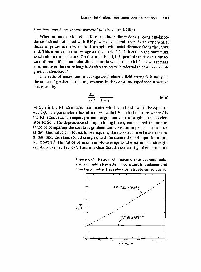
Constant-impedance vs constant-gradient structures (RBN)
When an accelerator of uniform modular dimensions (" constant-impe-dance " structure) is fed with RF power at one end, there is an exponentialdecay of power and electric field strength with axial distance from the inputend. This means that the average axial electric field is less than the maximumaxial field in the structure. On the other hand, it is possible to design a struc-ture of nonuniform modular dimensions in which the axial fields will remainconstant over the entire length. Such a structure is referred to as a " constant-gradient structure."
The ratio of maximum-to-average axial electric field strength is unity inthe constant-gradient structure, whereas in the constant-impedance structureit is given by
(6-6)1 -e~T
where T is the RF attenuation parameter which can be shown to be equal toojtF/2Q. The parameter T has often been called // in the literature where / isthe RF attenuation in nepers per unit length, and /is the length of the acceler-ator section. The dependence of x upon filling time tf emphasized the impor-tance of comparing the constant-gradient and constant-impedance structuresat the same value of T for each. For equal T, the two structures have the samefilling time, the same stored energies, and the same ratios of input-to-outputRF powers.3 The ratios of maximum-to-average axial electric field strengthare shown vs T in Fig. 6-7. Thus it is clear that the constant-gradient structure
Figure 6-7 Ratios of maximum-to-average axialelectric field strengths in constant-impedance andconstant-gradient accelerator structures versus r.

110 G. A. Loew et al.
-CONSTANT-IMPEDANCE
-CONSTANT-GRADIENT (Ez = CONSTANT)
O.I O.2 0.3 O.4 O.5 0.6 0.7 O.B 0.9 I.O
Figure 6-8 Axial field strength versus z/l for equal electron en-
ergy gain in constant-gradient and constant-impedance sections.
can produce higher electron energies than an optimized constant-impedancestructure when both are operating at the breakdown limit of electric fieldstrength. As indicated in Fig. 6-7, the relative advantage of the constant-gradient accelerator in achieving high gradients without breakdown dependsupon the value of r. Curves of field strength vs axial distance z for the twotypes of structures are shown in Fig. 6-8 for T = 0.57.
In addition to the advantage of the reduced ratio of maximum-to-averagefield strengths, the constant-gradient structure has several other advantagesover the constant-impedance structure:
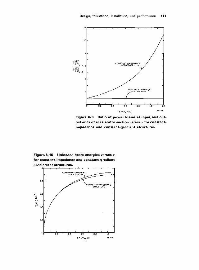
1. The power dissipated per unit length in the constant-gradient acceleratoris constant over the entire length of the structure. In contrast, the ratioof power loss at the input end to that at the output end of a constant-impedance structure may be as high as 12.4 to 1. (This magnitude corre-sponds to a value of the RF attenuation constant T = 1.26 Np, whichgives maximum no-load energy in the constant-impedance acceleratorstructure.) A plot of the power-loss ratios for the two structures is shownin Fig. 6-9.
2. The constant-gradient structure gives a slightly higher no-load beamenergy than the constant-impedance structure and somewhat lower beam-loading derivative (—dV/di). Thus, the constant-gradient structure hasgreater relative energy advantage in the loaded case than in the unloadedcase. The no-load energies for the two structures are shown in Fig. 6-10and the beam-loading derivatives in Fig. 6-11.
3. The constant-gradient structure has a higher maximum conversion effici-ency (ratio of maximum electron beam power to input RF power) and ahigher corresponding maximum peak beam current than the constant-impedance structure. Curves of the maximum conversion efficiency, »/max,and the corresponding maximum beam current, in , are shown in Fig.6-12.
4. The constant-gradient accelerator is less frequency-sensitive than theconstant-impedance accelerator, as shown in Fig. 6-13.
Design, fabrication, installation, and performance 111
O.2 O.4 O.6 O.8 I.O 1.2
Figure 6-9 Ratio of power losses at input and out-put ends of accelerator section versus r for constant-impedance and constant-gradient structures.
Figure 6-10 Unloaded beam energies versus rfor constant-impedance and constant-gradientaccelerator structures.

112 G. A. Loew et al.
0.2 O.4 O.6 0.8 1.0 \.Z
Figure 6-11 Beam loading derivatives versus T forconstant-impedance and constant-gradient accelera-tor structures.
Figure 6-12 Maximumbeamconversionefficienciesandcor-respondingvaluesof peak beam current versusr for constant-impedance and constant-gradient accelerator structures.
(CONSTANT-IMPEDANCESTRUCTURE

Design, fabrication, installation, and performance 113
Figure 6-13 Frequency sensitivities versus T forconstant-impedance and constant-gradient ac-celerator structures.
The factors discussed above depend upon T, as shown in Figs. 6-7through 6-13. To illustrate these factors numerically, the characteristicsof the two structures are shown in Table 6-3, based upon the parametersof the two-mile accelerator.
5. Amplitude and phase oscillations of the traveling wave caused by theband-pass filter characteristics of the structure may be slightly less pro-nounced in the constant-gradient than in the constant-impedance struc-ture (see Fig. 6-14). This problem was first pointed out in Reference 4and will be discussed in greater detail at the end of this section.
6. At the time the two-mile accelerator was being designed, the cumulative,multisection type of beam breakup described in detail in Chapter 7 was notknown. On the other hand, experiments done at Stanford and elsewhere5"8
had shown that the constant-gradient structure was relatively less troubledby the regenerative type of beam breakup than the constant-impedancestructure. Various laboratories had reported beam breakup thresholdswhich were typically of the order of 300 mA with a 2-^sec pulse lengthfor an S-band constant-impedance structure. At Stanford, it had beenfound that the instability could be triggered in a constant-impedancesection with a current of 70 mA by injecting about 800 W of power at4326 MHz backward into the output of the accelerator. However, thesame result had not been achieved with an equal amount of power in-jected into a constant-gradient section of the same length, showing that the

114 G. A. Loew et a/.
Table 6-3 Comparison of constant-gradient andconstant-impedance accelerator structures
Characteristic
E0 /Peak elec. field^V0/l \Avg. elec. field/
(dPldz),m0
(dP/dz)z=l
V0 (no-load energy)
-dVldiV (at i = 50 mA)^max (maximum beam-
conversion efficiency)
'•(max
Vg/c (normalized groupvelocity)
tF (filling time)U (stored energy)AZ = I (phase shift for
8/= 0.1 MHz)SF0/Fo(forS/=0.1 MHz)
Constant gradient
1.00
1.00
22.34 GeV35.53 GeV/A20.56 GeV
0.73
314.2 mA0.0204-^0.0065
0.83jLisec2372 J0.52 rad
0.033
Constant impedance
1.31
3.13
22.04 GeV36.41 GeV/A20.22 GeV
0.70
302.6 mA0.0121
0.83 jttsec2372 J
0.52 rad
0.039
Ratio" ^YIfffm
0.76
0.32
1.010.981.021.05
1.041 .68 -> 0.54
1.001.001.00
0.85
Assumed parameters:T = 0.57POT = 5320 MW (90% of which enters accelerator)L = 10,000 ft (94.8% effective)No. of sections = 960/=2856 MHzr = 53 megohms/meterQ = 13,000" e.g.—constant gradient; c.i.—constant impedance.
Figure 6-14 Shapes of input and outputRF pulses in constant-gradient (C.G.) andconstant-impedance (C.I.) acceleratorsections. Length of section = 10 ft,T = 0.57, and 2-77/3 mode in each case.Rise time of input pulse w0.1 jiisec; timescale = 0.2ju,sec/cm.
//4tJ
T\•H-H- 4+H -H-H-
/I
4*nH+i\\ ^—^
4+H- I I I 1*-'̂
•H44- -H-H-
j C.6.STRUCTURE
j C.I. STRUCTURE

Design, fabrication, installation, and performance 115
threshold must have been higher. An experiment done elsewhere9 showedthat by using a 5-ft long section of the Stanford constant-gradient design,thresholds as high as 600 mA in 3 ̂ sec had been observed. All these resultswere qualitatively understood at the time in terms of the HEM11 disper-sion diagrams which had been obtained and appear in Fig. 7-29. Indeed,in the backward-wave oscillator model, the frequency at which thevp = c line intersects the HEMn dispersion diagram changes over a wideband along a 10-ft section, rather than being constant as in the constant-impedance structure. Thus buildup of the backward-wave instability isless likely to occur. Furthermore, since the currents planned at SLACwere much lower than the obseryed thresholds, it appeared that theconstant-gradient design was assured of a reasonable degree of conserva-tism. As will be discussed in Chapter 7, if the accelerator were to be rede-signed today, one would probably stagger accelerator sections of differentdesigns along the 2-mile length in order to shorten the cumulativeHEMn interaction length at any given frequency. However, even withhindsight, it can be said that the choice of the constant-gradient designper se was correct from the beam breakup point of view since use of theconstant-impedance structure, with uniform interaction along each 10-ftlength, would have resulted in multisection breakup thresholds at evenmuch lower currents than have been observed at SLAC.
The advantages of the constant-gradient accelerator discussed abovehad to be weighed against two disadvantages: (a) Nonuniform modulardimensions made the cavities in the constant-gradient structure more expen-sive to fabricate and to test. An economic comparison of the two structuresshowed that fabrication of the constant-gradient structure cost approximately10% more per unit length than the constant-impedance structure, (b) Atthe time when the selection had to be made, there had been less operationalexperience with the constant-gradient structure than with the uniformstructure.
It was concluded that the advantages of the constant-gradient structureoutweighed its slightly higher fabrication cost. The constant-gradient struc-ture was thus adopted for the two-mile accelerator. Subsequently, high-power tests and actual beam tests conducted with sections installed in theMark IV and Mark III accelerators confirmed the theoretically predictedperformance.
Choice of attenuation parameter (RBN)
The attenuation parameter is defined as the net attenuation in nepers in anaccelerator section caused solely by resistive wall losses. It is equal to theproduct of the voltage attenuation per unit length and the length of theaccelerator section and is designated by the symbol T. As stated previously,T = a)tF/2Q, where CD is 2n times the operating frequency, tF is the filling time,and Q is the loss factor in the RF structure. As will be evident in the following

116 G. A. Loew et al.
L = IO.OOO (94.8% EFFECTIVE)
960 = NUMBER OF SECTIONS
r -- 53 MEGOHMS/METER
( = 2856 MHz
0 = I3.OOO
160 200 240
(MILLIAMPERES)
Figure 6-15 Beam loading curves for constant-gradientaccelerator at various values of the attenuation parameter r.
discussion, the value of ? influences the performance of a linac in many waysand, therefore, the proper choice of this parameter was quite important inthe design of the two-mile accelerator.
The total steady-state energy gain VT in a constant-gradient acceleratorof total length L and shunt impedance r0 is given3 by
ir0L (6-7)
where PT is the total input RF power, V is the peak beam current, and r0 isthe shunt impedance per unit length.
The first term on the right in Eq. (6-7) is the no-load energy (i.e., theelectron energy at negligible current), and the second term gives the reductionin energy caused by beam loading. The reduction of energy is linear withincrease in beam current, as shown in Fig. 6-15. In plotting these curves it isassumed that the electrons are situated at the peak of the traveling wave.
In the discussion which follows, the effect of T upon the constant-gradientaccelerator performance will be considered. The various accelerator charac-teristics are shown numerically in Table 6-4 for several values of T.
BEAM LOADING CHARACTERISTICS. Beam loading curves for the various valuesoft under consideration are shown in Fig. 6-15. The terminal point on eachcurve is the beam current resulting in maximum transfer of RF power to thebeam. As noted, the slope { — dV[di} of the beam loading curves decreases inmagnitude as T decreases. Since electrons with energies from VTQ to VTi
emerge from the accelerator during the transient period, lower values of iare preferred to reduce the energy spread.

Design, fabrication, installation, and performance 117
Table 6-4 Calculated performance of constant-gradientaccelerator at various values of attenuation parameter r
Characteristic
(Fro) Unloadedenergy (GeV)
(—dVldi) Beam loadingderivative (GeV/A)
(Fr<) Energy at 50-mAbeam current (GeV)
(AK)t transient energyspread (in GeV)between / = 0 andi = 50 mA
(*«niax) Beam current atmaximum conversionefficiency (mA)
(AK)e Energy loss inidle 10-ft section atz = 50mA (MeV)
(Vg/c) Normalizedgroup velocity"
(tF ) Filling time (jiisec)(-8V/V) Energy loss
forS/=0.1 MHz
0.4
20.10
26.59
18.76
1.34
377.8
1.32
0.0252-0.01 1 3
0.580.018
0.57
22.34
35.53
20.56
1.78
314.2
1.76
0.0204-0.0065
0.830.033
r(Np)
0.8
24.20
45.58
21.92
2.28
265.4
2.26
0.01 74-0.0035
1.160.056
1.0
25.18
52.61
22.56
2.62
239.4
2.60
0.01 60-0.0022
1.450.077
1.2
25.82
58.24
22.92
2.90
221.6
2.88
0.0152-0.0014
1.740.098
Assumptions:27T/3 mode, constant-gradient designPOT = 5320 MW (90% of which enters accelerator)L = 10,000 ft (94.8% effective)No. of sections = 960/=2856 MHzr = 53 megohms/meterQ = 13,000" The group velocity in each 10-ft accelerator section varies linearly between the limits given in each column.
MAXIMUM CONVERSION EFFICIENCY. The maximum conversion efficiency ofRF power to beam power is given3 by
-2 t 2(i - e-2t)
(6-8)
Maximum conversion efficiency occurs when the beam current reaches thevalue3
in which case the beam energy is equal to one-half of the no-load energy.

118 G. A. Loew et al.
ENERGY LOSS AND POWER INDUCED WHEN THE BEAM PASSES THROUGH SECTIONS
NOT SUPPLIED WITH RF POWER. When one of the klystrons along the accelera-tor becomes defective, it is desirable to be able to continue operation whilethe klystron is being changed. The amount (AKe) by which the electron beamenergy is reduced by excitation of an idle accelerator section of length / andthe induced power Pe in this section is given3 by
The energy loss increases as i increases, as shown in Table 6-4. Since each RFsource supplies four accelerator sections during Stage I operation, the totalenergy loss given by Eq. (6-10) must be multiplied by 4. This loss must, ofcourse, be added to the loss of beam energy incurred by the loss of the klystron(about 80 MeV under normal operating conditions).
GROUP VELOCITY. In the constant-gradient accelerator, the group velocitydecreases linearly with distance along the accelerator section. It is given3 by
FILLING TIME. A small filling time is desirable to allow the maximum avail-able portion of the RF pulse length for the acceleration of electrons. Thefilling time is given3 by
tF = — x (6-12)o>
Values of filling time for the various cases are given in Table 6-4.
FREQUENCY SENSITIVITY. The fractional beam energy loss from a fractionalfrequency shift <5///is given3 by
Values of 5V0/V0 are shown in Table 6-4 for Sf= 0.1 MHz.
CONCLUSIONS. From Table 6-4 it was clear that there were several advantagesto using a reduced attenuation parameter i. Except for the reduction in beamenergy, the use of a low value of T resulted in improvement of all of thefactors measuring the performance of the accelerator. Moreover, the percent-age improvement of each of these factors resulting from a given reduction

Design, fabrication, installation, and performance 119
in T usually exceeded the percentage loss in beam energy. In fact, if it werenot for the paramount importance of high beam energy in particle physicsresearch, the adoption of an even lower value of T would clearly have beenindicated. In conclusion, the choice of T = 0.57 was made on the basis ofbroad considerations, including reference to such tabulations as shown inTable 6-4, the prospective requirements of physics research, and previousaccelerator experience.
[The original basis for the exact value of T = 0.57 was that this particularvalue resulted in a no-load energy in the constant-impedance accelerator of10 % less than the maximum no-load energy which can be obtained (occurringat T = 1.26). This was judged to be the maximum penalty in energy whichone could afford to pay to obtain the advantages of low T discussed in thetext. The same qualitative reasoning held for the constant-gradient accelera-tor structure, and thus the value of T selected earlier was not changed.]
Transient filter characteristics and beam loading (RHH)
PHYSICAL MODEL AND EXPERIMENTAL EVIDENCE. The band-pass filter charac-teristics of the accelerator structure, which were discussed briefly earlier inthis chapter, will now be examined in greater detail. Both the physical modeland the theory will be presented below. As already mentioned, one effect ofthese filter characteristics is that an impressed RF wave of finite rise timeundergoes amplitude and phase oscillations as it travels down the acceleratorstructure. The impressed wave can come from the klystron or from beamloading. The oscillations which were illustrated in Fig. 6-14 can be under-stood in a simple way if one considers the symmetrical side-bands ± A/ ofthe carrier frequency (2856 MHz in this case) which are generated by the risetime of the RF wave. For an operating mode which is close to the middle ofthe CD — ft diagram (see Fig. 6-21), the small side-band vectors rotate aroundthe tip of the carrier vector in opposite directions but with approximatelyequal angular velocities. The resulting effect as a function of time and ofdistance along the structure is predominantly amplitude modulation becausethe sum of the two vectors remains approximately collinear with the carrierbut varies in amplitude. As the operating mode gets closer to the edge of thepassband, as in the 2n/3 case, both amplitude and phase modulation becomemore apparent.
The effect of this modulation on the beam is to cause spectrum broadening.In a multisection accelerator, this spectrum broadening can be reduced bynot triggering all the klystrons at exactly the same time, thereby causing the" peaks " and " valleys " to average out over a large number of sections.
Certain precautions should be taken when interpreting the pulse shapes ofFig. 6-14. It should be remembered that these pulses represent electric fieldamplitudes obtained at the end of a 10-ft section and that the electron beamenergy results from the integral taken over the full length. Experiments done

120 G. A. Loew et a/.
by probing the field through small coupling holes drilled along a 10-ft sectionshow that the evolution of the pulse shapes as a function of length is morecomplicated in the constant-gradient structure than in the constant-impedancestructure. In addition to the side-bands caused by the rise time of the pulse,there is a frequency modulation effect. This frequency modulation is inherentin the rise time of the pulsed klystron supplying the RF power. At turn-on,the frequency can in fact be several megahertz higher than when the flat topof the modulator pulse is reached. This initial energy, which travels down theaccelerator structure at a higher frequency, reaches an increasingly narrowpass-band structure as seen in Fig. 6-21. Before being attenuated, this energytravels at a group velocity which is much lower than the corresponding groupvelocity at 2856 MHz. When the pulse shape is examined in the middle of thesection, the wiggles do not die out, i.e., the filling time is at least 2.5 micro-seconds long. Finally, towards the coupler end, the higher frequency energygets attenuated or reflected and the pulse looks more and more like the simpleoutput shown in Fig. 6-14. Because of the presence of the higher frequencies,the frequency of the wiggles is about twice as high at the input as at the out-put. While this effect is probably unimportant, experiments have shown thata 50 % reduction in ripple amplitude can be obtained if a diode modulator atlow power, preceding the klystron, is used for RF turnon. This result can beunderstood by the reduction in frequency modulation obtained with thep-i-n diode as compared with the klystron alone.
COUPLED RESONATOR WAVE EQUATIONS. The transient phenomena of wavepropagation and beam loading can be described approximately by a simpletheory in which the disk-loaded waveguide is treated as a continuous trans-mission line of which the dispersive properties are characterized by a well-defined group velocity. As has been pointed out by J. Leiss,4 however, such
Figure 6-16
waveguide.
Mathematical model of a disk-loaded

Design, fabrication, installation, and performance 121
a treatment overlooks important transient effects arising from the finite pass-band of the periodically loaded structure.
The approach used here is an approximate version of coupled-resonatortheory, equivalent to the filter-network approach of Reference 4. The waveequation may be written* (see Fig. 6-16 for geometric nomenclature):
t—2 + 2pn — + C^J/UT) - con jnn_1 / 2xn_^T + -j + nn + 1 / 2^n + 1^T - -
= -f <A*(rV2(r',T--WY (6-14)Un
Jcavity \ V)
where
An(t) is related to the vector potential in the nth cavity by A »^n(T)v|/n(r'),
\l/n(r') is the characteristic spatial distribution of the vector potentialin the nth cavity,
<//zn(r') is the z-component of vj/n,
r = t— \ " dz/v(z) is the "local" time, retarded by electron transit
time,a)n is a characteristic frequency parameter (the midband frequency),fin = ^a)JQn is the loss coefficient,^n+i/2 is a measure of the coupling between the nth and (n ± l)th
cavities,
un = |\J/n(r')|2 d3r' (proportional to stored energy); and
Jcell
Jz(r', T) is the current density, assumed to consist of electrons travelingin the ± z direction at velocity v.
The assumptions that the parameters /?„, a>n, and £)„ are simple sealers isstrictly valid only in the weak-coupling (small-hole) limit.
The equation may be interpreted phenomenologically by noting that, ifthe parameters vary only adiabatically as a function of n, then the homogene-ous part has solutions of the form
A ~ A p~ik"dAn ~ An-\e
where an implicit el(aT is understood, and
wl + 2i/ln co-co2x 2con Qn cos kn d (6-15)
Thus, if one assumes
fin « a>n and QB ̂ a>n
the dispersion formula is a cosine-like curve with a>n the midband frequencyand Qn approximately the half-bandwidth.
* In the present discussion, the units are Gaussian with c=\, unless otherwise noted.

122 G. A. Loew et al.
An even simpler dispersion relation results if one assumes |(co — con)/wn | <^ 1 ;i.e., that the fields have no frequency components very far from +(on; onemay then write
<°n + Pn — W ~ ^n COS &n ^ (6-16)
In this case the wave equation may be written
J «r 'Vzr ' ,T--dV (6-17)lCOnUn J cavity \ V/
APPLICATION TO ACCELERATOR MODE. In the accelerator mode, the longitud-inal field is transversely uniform near the axis, e.g.,
^ « «AZ(O, o, z')
Defining the complex voltage gain, wn(r), by
cavity(6-18)
or, assuming an instantaneous variation ~elu>nr, and noting that Ez «— i(on Az , one may write
wnW*-iconFnAnW (6-19)
where
Fn = ! ^(z'^'"* dz' (6-20)•^cavity
The voltage gain for an electron entering the structure at time t = t is
F(T) = lRewn(T)i
The wave equation (Eq. 6-17) may now be written
(6-21)
1 (Qn_1/2 W^^T) + fin+1/2 wn+1(T)} « -pnRn
(6.22)where /(T) is the beam current ;
and Rn , the shunt impedance per cavity, is defined by
Rn_2pnRn_4n\Fn\2
— — - — --Qn <°n 0)n Un

Design, fabrication, installation, and performance 123
Figure 6-17a Field distribution in the acceleratingmode along a constant-gradient structure, 0.6 jusecafter turning on a unit step-function driving voltagein the zeroth cavity.
The transient behavior of typical disk-loaded guides has been investigatedby a computer program which integrates Eq. (6-22). The program data inputprovides for arbitrary longitudinal variation of the waveguide parametersand choices of appropriate boundary conditions, driving sources, and beammodels. As a computational convenience, the program actually calculatesthe function Wn(r), defined by
where a>' is a constant reference frequency (e.g., the driving source frequency)and Wn(r) is slowly varying in phase and amplitude.
Figures 6-17 and 6-18 show the results of typical computations based onthe properties of the SLAC structure. The table below summarizes the per-tinent initial and final values of the parameters :
Cavity No.
085
Vg/C
0.02040.0061
Q/27T
(MHz)
32.010.41
Q
14,1701 3,220
Rid(megohms/ meter)
5360
124 G. A. Loew et al.
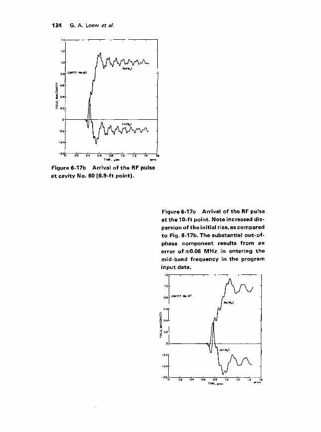
Figure 6-17b Arrival of the RF pulseat cavity No. 60 (6.9-ft point).
Figure 6-17c Arrival of the RF pulseat the 10-ft point. Note increased dis-persion of the initial rise, as comparedto Fig. 6-17b. The substantial out-of-phase component results from anerror of &0.06 MHz in entering themid-band frequency in the programinput data.

Design, fabrication, installation, and performance 125
Figure 6-18 Electron energy gain versus time cor-responding to the case of Figs. 6-1 7a, b, and c. Thelarge ripples seen in the field plots have nearly aver-aged out in the summation over the cavities.
The values of half-bandwidth, Qn , used in the computation are derivedfrom the design group velocity, vg(n), through the relation
a9 dk
A step-function driving voltage applied at time T = 0 at the input boundarywas assumed in all the computations. Physically, such a step function wouldbe closely approximated by means of the p-i-n diode mentioned earlier. It isseen that these computations are in excellent agreement with the experimentalobservations mentioned above. Comparing Figs. 6-17b and 6-17c, it is seenhow the wiggles evolve as a function of length, as the group dispersionincreases. As the pass-band becomes narrower, certain frequency compo-nents which are shock-excited by the step-function driving voltage are reflectedfrom the 0- or 7r-mode band edge at some point down the structure, propagateback to the input where they are again reflected by the constant voltagesource (zero impedance) and thus set up standing-wave resonances. Suchresonances would probably be much less noticeable in a more realistic casewith finite rise time and source impedance matched to the guide. The appear-ance of a^significant out-of-phase component of the field (Fig. 6-17 'c) resultsfrom a slight input data error of «0.06 MHz in the midband frequency. Asa result, the wave is not quite synchronous at the assumed bunching frequencyof 2856 MHz.
In conclusion, it is seen from Fig. 6-18 that the variation in electron energygain is at most 1 % at the beginning of the beam pulse and that it rapidlydecreases from then on. Measurements made with a short accelerator lengthhave confirmed these results.

126 G. A. Loew et al.
6-2 Empirical design of the accelerator structure
Choice of the disk-loaded waveguide (GAL)
The first section of this chapter was concerned with the general determina-tion of accelerator parameters. This section describes the procedures used todesign empirically an accelerator structure that satisfies the above parameters.
The disk-loaded waveguide is not the only slow-wave structure capable ofaccelerating electrons. In fact, other structures (see Fig. 6-19) such as thegrid-loaded ("jungle gym") waveguide yield shunt impedances about twicethat of the disk-loaded waveguide. But in every case that was examined,where a large improvement in shunt impedance was obtained, the bandwidthand resulting group velocity were at least 10 times as high as desired. Efficientutilization of the available RF power under these conditions would have
Figure 6-19 Slow-wave structures
proposed for linear accelerators.FORWARD-WAVE STRUCTURES
I. DISK-LOADED STRUCTURE 2. VENTILATED STRUCTURE
3. CENTIPEDE STRUCTURE 4. RECTANGULAR SLAB
BACKWARD-WAVE STRUCTURES
S.'UUNGLE GYM" 6. SLOTTED DISK STRUCTURE
7. RING & BAR STRUCTURE 8. LOADED EASITRON

Design, fabrication, installation, and performance 127
required its recirculation (feedback) or the use of extreme lengths betweenfeeds. The former was undesirable, especially in a long multisection acceler-ator, because it would have resulted in undue operational complications;the latter would have required that each accelerator section transmit anexcessive amount of power. Several variations of structures 2 through 8shown in Fig. 6-19 were devised which succeeded in reducing the groupvelocity to the desired values (in the range of O.Olc), but these measures alsocaused the shunt impedance to be reduced until no advantage remained;moreover, they would have resulted in increased cost of fabrication. For thesereasons, the disk-loaded waveguide was preferred for the two-mile accelerator.
Definition and discussion of dimensions (GAL)
The modular dimensions of the disk-loaded waveguide which can be adjustedto achieve the intended parameters have already been illustrated in Fig. 6-2.Figure 6-2a and b shows the cylindrical guide diameter 2b, the disk-hole di-ameter 2a, the disk-edge radius p, and the land in the disk aperture s. Figure6-2c shows further variations of the disk-loaded waveguide using so-called"conical" or "anticonical" disks. The conical disk was rejected because ofits comparatively low r/Q. The anticonical disk was dismissed because ofmachining difficulties, although it has a 5% higher r/Q than the correspond-ing flat dislc structure with t = t^= 0.230 in.
As indicated earlier, a 10% improvement in shunt impedance was gainedby adopting the 2n/3 mode rather than the ii/2 mode. Figure 6-20 illustrates
Figure 6-20 Traveling-waveelectricf ield configur-ations for 0, 7T/2, 27T/3, and77 phase shift per cavity.
laooooaac
27T3

128 G. A. Loew et a/.
the respective traveling-wave field configurations at an instant in time overtwo wavelengths (the zero and n " standing-wave modes " are also illustratedfor reference). These patterns are deformed as they slide down the waveguidebut reappear in the same configuration, shifted by one cavity, at an instant5t = <f)/2nf later, where </> is the phase shift per cavity at the frequency/.
For standard accelerator sections, the objective is to obtain a phasevelocity equal to the velocity of light. Thus, specifying the operating modeand frequency (or free-space wavelength) fixes the distance between diskcenter lines at d = (f)c/a>. After this choice, only four dimensions remain tobe specified: 2b, 2a, p, and t. The lower cutoff frequency of the disk-loadedwaveguide, or "zero-mode" frequency, is strongly dependent upon thewaveguide diameter 2b, whereas the bandwidth and, thus, the group velocitydepend primarily on the ratio a/b at given values of p and t. This point isillustrated by the three w-fi (Brillouin) diagrams shown in Fig. 6-21. Forexperimental tests and later, in the fabrication, it was important to verifythat the disk aperture edge had been properly formed; this was done throughsome technique such as that utilizing a steel ball (Fig. 6-2b) or a more
Figure 6-21 Brillouin diagrams for three differentpoints in a typical constant-gradient section.
U) vs /3d ATz~o; z~6', AND z~!O'IN A CONSTANT-GRADIENT STRUCTURE
/3d (RAD)

Design, fabrication, installation, and performance 129
sophisticated contour plotter. Errors in the ball height h or the land s causesignificant errors in the resonant frequency of test sections and hence in theresulting phase and group velocities. This fact is easily understandable becausethe electric field intensity is relatively strong at the disk edge. The choice of pcan be quite arbitrary from the RF point of view so long as the tolerances arerespected and electric breakdown does not result.
The choice of the disk thickness t, as discussed in the previous section,involve a compromise between the use of thin disks to increase the shuntimpedance and thick disks to reduce the danger of electrical breakdown,improve heat-transfer characteristics, and increase mechanical strength.
Evolution of Stanford designs (GAL)
Prior to 1960, all Stanford accelerators had been designed to operate in the7T/2 mode. Starting in 1960, the first 2n/3 mode structure was tested on the20-ft Mark IV accelerator. Until 1962, all Stanford accelerators were of theconstant-impedance type. Then, in April 1962, the first constant-gradientstructure was installed on the Mark IV accelerator. Finally, SLAC-typeconstant-gradient structures were installed on the Mark III accelerator inDecember 1963, replacing the earlier n/2 structures.
Table 6-5 shows a recapitulation of the respective characteristics of con-stant-impedance structures operating in the n/2 mode on the early Mark IIIaccelerator and in the 2n/3 mode on the Mark IV accelerator.
Table 6-5 Characteristics of Stanford constant-impedance structures
Mark III accelerator Mark IV acceleratorParameters (1952) (1960)
Operating modeLength (ft)Waveguide inside diameter 2b (in.)Disk hole diameter 2a (in.)Disk thickness t (in.)Periodic length d (in)Disk edge radius p (in.)Matching iris aperture (in.)Frequency (MHz)Group velocity vg/cShunt impedance r0 (megohms/
meter) (corrected for funda-mental space-harmonic ampli-tude)
QAttenuation T (Np)
77/2
10
3.2470.82250.2301 .03350.12151.04228560.01 00
47
10,0000.90
27T/3
10
3.2470.8900.2301.3780.12151.01428560.0122
53
13,2000.57

130 G. A. Loew et a/.
Constant-gradient structure dimensions (GAL)
As already discussed, the two-mile accelerator is of the constant-gradienttype, propagating in the 2n/3 mode. The constant field is obtained by taperingthe cross-sectional dimensions of the waveguide so as to produce the requiredlinear decrease in group velocity. The constant-field condition then resultsonly if the shunt impedance and the Q of the cavities remain constant over thelength of the section in spite of the cross-sectional variation of the structure.In practice, for a group velocity variation such as that chosen for the SLACdesign, the shunt impedance r0 (corrected for the fundamental space har-monic) increases by a small percentage over a 10-ft section, thereby yielding astructure with a gradual input-to-output field increase of 5 %. Then, in thepresence of beam loading, the rising field characteristic is compensated for,as will be seen later in this section.
Two constant-gradient structures were designed, one for thick disks(t = 0.230 in.), the other for thinner disks (t = 0.120 in.). Their performanceswere compared and the thicker disk design was chosen for the reasons alreadymentioned earlier. Figures 6-22 and 6-23 show the respective variations of2b, la, vjc, and r0 as a function of cavity number along a 10-ft section.
Figure 6-22 Variation of 2b. 2a, vg/c, and the shunt impedance r0 (correc-ted for the fundamental space harmonic) as a function of cavity numberalong a 10-ft constant-gradient section for t = 0.230 in. The values of 2band 2a in this figure are those given in Table 6-6. These final values wereobtained by applying several corrections to the cold test data, includingthose given by Eqs. (6-44) and (6-45).
CAVITY NUMBER FROM INPUT END

Design, fabrication, installation, and performance 131
CflVITY NUMBER FROM INPUT END
Fig. 6-23 Variation of 2b, 2a, vg/c, and the shunt impedance r0 (correctedfor the fundamental space harmonic) as a function of cavity numberalong a 10-ft constant-gradient section for / = 0.120 in.
Cavities 0 and 85 are coupler cavities. It is seen that whereas 2b varies byless than 2%, la is reduced at the output by 30% from its input value tosatisfy the group velocity variation.
When economy in fabrication is desired, a constant-gradient design canbe approximated by adjusting the dimensions in steps, each step consistingof several identical cavities. However, for the two-mile Stanford accelerator,the cost of the slow-wave structure represented only a small percentage ofthe total cost, and the small increase incurred by varying the dimensionscavity by cavity was well justified to achieve a smooth field gradient.
Cold tests and corrections to achieve the empirical design (GAL)
OBJECTIVES AND VALIDITY OF COLD TESTS. A computer program sufficientlyaccurate to permit calculation of the dimensions of the constant-gradientdesigns shown in Figs. 6-22 and 6-23 did not exist at the time. Consequentlythese dimensions had to be determined experimentally from cold tests. Toachieve an accurate design, a fair number of pairs of 2b and la values had tobe determined, each set of values being obtained from a different resonanttest cell. About ten different test cells were used for each of the constant-gradient designs. For each test cell, the following quantities were measured:the phase velocity vp, the group velocity vg, r/Q, Q, and the fundamental
132 G. A. Loew et al.
space harmonic amplitude «o/Zan- The detailed description of these micro-wave measurements is beyond the scope of this book. Comprehensive treat-ments of this subject can, for example, be found in References 2, 10, and 11.However, a brief comment is made here on each of these measurements tooutline the techniques that were used and the precautions that were taken.A discussion of the corrections applied to the experimental results is alsoincluded.
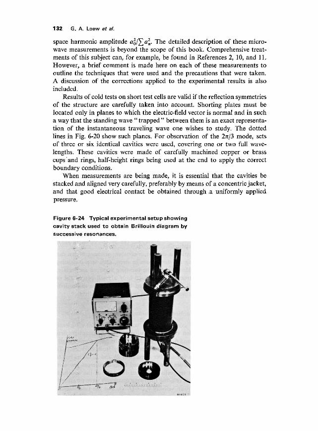
Results of cold tests on short test cells are valid if the reflection symmetriesof the structure are carefully taken into account. Shorting plates must belocated only in planes to which the electric-field vector is normal and in sucha way that the standing wave " trapped" between them is an exact representa-tion of the instantaneous traveling wave one wishes to study. The dottedlines in Fig. 6-20 show such planes. For observation of the 2n/3 mode, setsof three or six identical cavities were used, covering one or two full wave-lengths. These cavities were made of carefully machined copper or brasscups and rings, half-height rings being used at the end to apply the correctboundary conditions.
When measurements are being made, it is essential that the cavities bestacked and aligned very carefully, preferably by means of a concentric jacket,and that good electrical contact be obtained through a uniformly appliedpressure.
Figure 6-24 Typical experimental setup showingcavity stack used to obtain Brillouin diagram bysuccessive resonances.

Design, fabrication, installation, and performance 133
MEASUREMENT OF PHASE VELOCITY vp. The graph in Fig. 6-24 illustrates atypical Brillouin diagram with the phase velocity vp = c for a 2rc/3 phaseshift per cavity at/= 2856 MHz. The disk spacing was fixed at A/3 = c/3f=104/2856 cm. With three or six cavities of the type shown, four or sevenresonant frequencies, respectively, representing nn/3 (0 < « < 3) or nn/6(0 < n < 6) phase shift per cavity, can occur; these points were recorded todraw the co-fi diagram. With a moderate amount of experience, three roundsof machining correction of the diameter 2b were sufficient to approach theoperating frequency (2856 MHz) within less than 1 MHz at 2n/3 resonance.The remaining correction was done by interpolation.
MEASUREMENT OF GROUP VELOCITY vg. The condition vg = c can be obtainedfor various pairs of 2b and la values. Each pair yields a different o>-/? diagramand, hence, a different group velocity. This fact has already been illustratedin Fig. 6-21. Figure 6-25 shows the two cavity stacks for the extreme cases,the first and the last cavities of the constant-gradient section. The differencesin 2a for vg/c = 0.0204 and vg/c = 0.0065 can be observed. To obtain the groupvelocity, the slope of the ca-f} diagram was measured and, for better accuracy,a Stirling or Fourier approximation formula12 was used with the measuredresonance frequencies.
Figure 6-25 Typical cold test setup showing cav-ity stacks and group velocity variation as a func-tion of length along a constant-gradient section.

134 G. A. Loew et a/.
MEASUREMENT OF r/Q. The ratio of shunt impedance per unit length to Qwas best measured by perturbing the axial fields in the cavity stack with a thindielectric rod and by measuring the resonant frequency perturbation A/.Using Slater's perturbation formula,11'13 the value of (r/Q)T (where theindex T denotes the sum of all space-harmonic components) is given by
^^(6'24)
where e is the dielectric constant of the rod (for sapphire e « 10), and A is itscross-sectional area. It was easiest to calibrate the dielectric rod in a simpleTM010 cavity, for which r/Q can be calculated.
MEASUREMENT OF THE SPACE-HARMONIC AMPLITUDE. Since only the fundamen-tal space harmonic propagates at vp — c, it alone gives a net energy gain tothe electrons. Thus, to obtain the effective (r/Q)0, it was necessary to obtainthe amplitude of the fundamental. The figure of merit by which to multiply(r/Q)T to obtain (r/Q)0 is a^/^al, the ratio of the square of the fundamentalharmonic amplitude divided by the sum of the squares of all harmonicamplitudes. This ratio was obtained by noting the frequency perturbationcaused by a short metallic or dielectric needle drawn along the axis of theresonant cavity stack. The field Ec at a given axial position in the cavity isrelated to the frequency perturbation A/caused by the needle located in thatposition by
E2C = k A/ (6-25)
where A: is a constant depending on the characteristics of the needle. For bestaccuracy, the following precautions were taken:
1. Needle lengths were kept between 5 and 9 mm to give adequate sensitivityand good resolution.
2. Six cavities were used so that an entire half-wavelength could be probedwithout letting the needle approach the end plates, where its image wouldincrease the actual perturbation.
3. The perturbed frequency was measured by adjusting the frequency tolocate the new peak of the response curve rather than by observing powerresponse as a function of needle position at constant frequency. Thistechnique avoided the difficulties14"16 which arise from simultaneouschanges in the resonant frequency and the coupling coefficients of thecavity.
4. Before plotting the whole field pattern, symmetry of the field was checkedby using the method described in (3) above for a few points symmetricalwith respect to points of reflection symmetry. Lack of symmetry wascorrected by adjustment of small tuning plungers at the top of the cavitystack. These plungers compensated for the asymmetry created by slightdifferences in insertion of the input and output coupling loops.

Design, fabrication, installation, and performance 135
After the field pattern was obtained, a Fourier analysis was carried out toobtain the figure of merit, which is given by
(6-26)2X I tV2EldzJo c
It was sufficient to divide the Ec pattern into twenty-one intervals andevaluate the integral using the trapezoidal approximation.
MEASUREMENT OF Q. This was the most difficult measurement to make be-cause the results depended on the state of the metal surface and the degreeof contact between cavities. Measurements were usually taken immediatelyafter electropolishing the cavities. Using very weak coupling, the £>'s of three-cavity (Q3) and six-cavity (Q6) sets were successively obtained by the half-power point technique :
Q=£j. (6-27)
where / is the resonant frequency and A/ is the frequency variation betweenhalf-power points. Although the Q's thus obtained were lowered by end-platelosses, the end effects were eliminated through use of the following expres-
The following precautions were taken when making Q measurements:(a) The signal generator was checked for spurious outputs, (b) The inputpower was carefully monitored, (c) To eliminate errors due to uncertaintiesin crystal law behavior at varying power levels or indicator calibrations,measurements were made at a constant crystal power level. This was achievedby using a precision attenuator which was adjusted from 3 to 0 dB as theresonant frequency and the half-power frequencies were sought. A finalcheck of the Q measurement was obtained by measuring the attenuation ofan accelerator section after final assembly.
ENVIRONMENTAL TEST CONDITIONS AND CORRECTIONS. In Order to build a
constant-gradient section with fixed ?, d, and p dimensions, only 2b and 2ahad to be obtained and their relationship with vp and vg had to be determinedaccurately. The quantities (r/Q)0 and Q did not have to be known so pre-cisely, because to a first approximation they do not enter into the design.
Measurements were carried out in an environment having accuratelycontrolled temperature and humidity. Since it was not practical to machine-test cavities to attain the exact design frequency, the final value of 2b had to

136 G. A. Loew et al.
be corrected for the residual A/. It was usually sufficient to base the correctionon the simple relation
A O t* ^ I*
- — « - — = -0.0011 in./MHz (at 2856 MHz) (6-29)
Another correction was required to arrive at the operating frequency for agiven copper temperature differing from the room temperature at which thetests were being performed. In addition, most cold tests were done in air, anda correction had to be applied for the dielectric constant of air, which is afunction of the ambient humidity and temperature (see Adam's nomographin any engineering handbook). These problems were not very critical forshort cavity-stack measurements but became important during matchingand tuning operations, as discussed in a later section. For copper, the follow-ing rule of thumb can be applied at 2856 MHz:
-^ = - 0.100 MHz/2°C (6-30)
Translation from air at 80° F and 40% humidity to vacuum results in afrequency increase of about 300 parts/million.
Having applied these corrections, the values of 2a and 2b were smoothed,first by plotting the points on a curve, and then by using a simple computerprogram to obtain a fourth-order fit.
Basic considerations in matching and tuning an accelerator section (GAL)
If the process of machining parts and fabricating an accelerator structurecould be carried out with perfect accuracy, a section such as the one shown inFig. 5-13 would be ready for installation and use immediately after fabrica-tion.
In practice, however, it is difficult to control the process of manufacturingto this extent; moreover, it is not economical to do so. By relaxing the toler-ances on the fabrication techniques described later in this chapter, it waspossible to reduce the cost of the accelerator considerably. The imperfectionswere corrected through the process of tuning and matching for a relativelysmall incremental cost.
The process of tuning an accelerator section consisted of applying externalmechanical pressure to impart a permanent deformation to the wall of anycavity of which the phase shift differed from the design value. In tuning, amaximum phase excursion of ±2.5° was allowed for the 10-ft sections of thetwo-mile machine.
Matching the couplers of an accelerator section was done by adjusting thedimensions of the input and output coupling irises (see Fig. 6-26) so as toinsure a low standing-wave ratio at the input and output of the structure. Anupper VSWR limit of 1.05 was set as the matching requirement for all coup-lers. The main technical difficulty stemmed from the fact that the processes of

Design, fabrication, installation, and performance 137
Figure 6-26 Sketch of a 10-ft long, constant-gradient, accelerator structure with inputand output couplers. Notice slight taper inmodular dimensions (diameter of inner wall).
tuning and matching are interrelated; the shape of the coupling iris deter-mines both the coupling to and the phase shift of the first cavity.
A complete description of the theory and operations involved in tuningand matching an accelerator section is beyond the scope of this chapter.Good discussions on these subjects can be found in References 2, 10, 11, and17-19. Only a few of the general principles and relevant precautions aregiven below.
Although the simplest mode to tune and match is the n/2, any submultipleof 2n, such as the 2n/3 mode, can be handled without undue difficulty.
Figure 6-27 illustrates the principle of the nodal-shift technique which
Figure 6-27 Principle of the nodal shifting technique. Shown atleft are the cutaway section with the copper plunger, and typicalSmith chart plot.

138 G. A. Loew et a/.
was utilized in tuning. A copper plunger, progressively pulled through thestructure (shown in cutaway section in the figure), detunes successive cavitiesand thereby causes the standing-wave pattern to shift. If the coupler is per-fectly matched and all cavities have 120° of phase shift (2n/3 mode), pullingthe plunger away from the coupler causes the plotted null points to rotateclockwise by 240 electrical degrees on the Smith chart for each cavity lengththrough which the plunger is moved. Starting from the reference point of 0°,obtained by detuning the coupler cavity (and, hence, representing the planeof the iris), the points move clockwise as shown in Fig. 6-27 from 0° to 120°,from 120° to 240°, from 240° to 0°, and so on. For the first cavities, the VSWRis nearly infinite and the points are on the rim of the chart. Farther down thesection, the VSWR decreases because of the increasing net attenuation be-tween the input of the section and the short. Thus, the plotted points movetoward the center of the chart along the three radii, shown as dashed linesin Fig. 6-27. With the coupler perfectly matched but the cavities not exactlytuned, the points move erratically toward the center, as shown by the heavylines. However, the center of the circle passing through three consecutivepoints still coincides with the center of the chart. When a systematic phase-shift error exists, because of an inaccurate choice of frequency, the pointsspiral in toward the center, clockwise if the phase shift is too large (frequencytoo high), or counterclockwise if it is too small (frequency too low). If thecoupler is mismatched (see Fig. 6-28), the circle passing through the threepoints is no longer concentric with the rim of the chart. It now has two"centers"—a geometrical center and a "Smith center." Neither coincideswith the center of the chart. The Smith center is the point that would beobtained if the perfectly reflecting plunger were replaced by a perfectlymatched load. It can be determined mathematically10'11 from geometricconsiderations. The match point (C) will lie on the extension of the straightline from the center of the Smith chart (O) to the geometric center of thecircle (M). Its VSWR (a at the match point) is determined by (amaj(rm\n)
l/2
if the circle encompasses the center of the chart, and by (crmaxo-mi-n)1/2 if it doesnot. Matching the coupler consists of bringing point C as close as possible topoint O. This is achieved by adjusting the coupling iris. Filing or squeezingaffects the coupling, but they also affect the phase shift of the coupling cavity.Bending the iris in or out can compensate for this change. For the example ofpoint C as shown in Fig. 6-28, the actions that must be taken are to bend theiris inward and to increase the iris opening by filing. In general, both bendingand filing are required to achieve a good match.
The process of tuning is illustrated in Fig. 6-29 for a short experimentalsection of accelerator pipe. The tuning tool here is being applied to the thirdcavity. It consists of a demountable collar with two or three radially adjust-able screws having rounded ends. By driving a screw into the wall of theaccelerator, a dimple is formed on the outer wall, resulting in a small pro-trusion from the inside wall of the cavity. To preserve cylindrical symmetry,it is best to obtain the desired phase shift with two or more dimples uniformly

Design, fabrication, installation, and performance 139
MATCHPOINT (C) MATCHPOINT (C) FROMTHREE SUCCESSIVESHORTING PLUNGER DATA
Figure 6-28 Smith chart plot obtained in the coupler-matching technique.
distributed around the circumference. Errors A(2b) in the dimension 2bcreate phase shifts A0 by
2nc= — - k3 r
(6-31)
where k x (1.0) MHz/0.001 in. For example, an error of 1° correspondingto a A(26) of 0.0002 in. can easily be eliminated. In practice, all cavities wereinitially machined to a diameter nominally 0.0005 in. oversize. This assuredthat after allowing for machining tolerances, the correct tuning of all cavitiescould be achieved by external dimpling, as described above.

140 G. A. Loew et al.
Figure 6-29 Experimental arrangement for tuning a shortaccelerator section, with illustration of tuning tool.
Because field lines can extend over a distance of three disks in the 2n/3mode configuration, tuning and matching strongly interact in the first cavities.It was pointed out20 that this property can cause serious difficulties. If thecoupler is not well matched, tuning the first cavities by bringing the points tothe proper positions on the Smith chart can actually cause the followingeffect: successive cavities will have built-in cyclic phase errors A^, A02 > A03
which compensate for the reflection caused by the coupler. Since the VSWRfor the nodal shift in the first cavities approaches infinity, the match point Cis indistinguishable from the center O of the Smith chart, and the structureappears to be tuned and matched. In reality, a double or triple perodicity isbuilt into the section, which causes passband splitting. It was predicted20
that the split would occur at approximately the n/2 frequency for a 2n/3section. Precautions can be taken to avoid this possible ambiguity. Oneremedy consists of using a resistive plunger which even in the first cavitiesallows the position of the match point C to be identified. Another techniqueis to measure the phase of the wave reflected from the coupler and the adja-cent (No. 1) cavity (assuming the dimensions of the latter cavity to be correct).By placing the tuning plunger alternately in cavities 1 and 2, the requiredcondition of 120° phase shift per cavity may be approached iteratively bydimpling the coupler cavity and filing the coupling iris. In practice, this resultwas achieved by separately prematching the couplers with a perfect three-cavity assembly before final brazing of the section. A particular technique toprematch the coupler without a perfect three-cavity assembly has also beenworked out21 for particular use with a structure operating in the 2n/3 mode.

Design, fabrication, installation, and performance 141
In this technique it is necessary to know the frequency at which each cavityhas 7T/2 phase shift. This method is useful in preventing any incorrect match-ing which could cause the incorrect tuning mentioned above.
A few additional remarks should be made:1. The matching and tuning operation must be performed in a carefully
temperature-controlled dry room. Sections should be allowed to stabilizethermally for several hours. Preferably, the tuning operation should be donewith the section filled with dry air.
2. The detuning plunger should be light and clean in order to preventdamage or contamination of the disk edges. Notches should be provided sothat the plunger always rests in the same relative position, or dwell point,around which small motions do not disturb the null. When tuning a constant-gradient section, where the 2a dimension changes as a function of length, thelargest possible plunger compatible with the smallest 2a dimension should beused. It was verified that, in this manner, the dwell condition can be achievedin all cavities.
3. In the 2n/3 mode it was found that moving the plunger by less than afull cavity away from the coupler causes the null on the slotted line to movetoward the generator by one-half the phase shift introduced. This surprisingeffect is attributable to the manner in which the plunger detunes the cavityand not to any actual phase reversal. When the plunger finally moves intothe dwell point in the next cavity, the null appears in the correct place.
4. Contrary to the early Mark III sections, the SLAC sections are pro-vided with output couplers and loads to prevent a reflected wave from appear-ing at the klystron amplifiers. These couplers had to be tuned in the samemanner as the input couplers, by switching over the whole experimentalsetup to the output coupler.
5. When an experimental section has been matched and tuned, three finalRF checks are advisable: (1) The global match can be checked with a con-tinuously movable short in the rectangular waveguide beyond the outputcoupler.11 This measurement involves observing the image of two inter-secting diameters on the Smith chart, transformed through the completesection including the two couplers. This image of the " iconocenter" mustfall at the center of the chart. (2) The global match can be checked with amatched load at the output or input ends. (3) The attenuation can be meas-ured globally for the entire section by direct substitution techniques, or for apart of the section by measuring the change in reflection coefficient as afunction of plunger position.
Finally, it is often of interest to obtain a complete traveling-wave fieldplot for the entire accelerator section. This plot can be obtained by drawinga small metallic or dielectric needle along the axis of a disk-loaded waveguidestructure which is excited at one end by a signal generator and matched at theother end with a load. The relative field amplitude is obtained by measuringeither the reflection coefficient caused by the reflected wave from the bead, orthe phase shift across the section caused by the forward-scattered wave from

142 G. A. Loew et a/.
the bead. The phase of the field can be measured by noting the phase of thereflection coefficient of the reflected wave.
It is interesting to note that if one wants to recheck the relative amplitudeof the fundamental space harmonic (flo/Z^n) ^v tn's method, both electricfield amplitude and phase are needed, as shown by the derivation below. Thetotal field is given by the expression
n= + oo
Ez(z,t)= Z a-C'OexppCajf-ft.z)] (6-32)n= — oo
where /?„ is the phase constant associated with the «th space harmonic. Inte-grating over the length of one cavity, one obtains
1 r + d/2
an = -\ E.(z) exp(//L z) dz (6-33)d J-d/2
Notice, however, that Ez in this expression is a complex quantity of the form\Ez(z)\e~je(z\ where the plots of \Ez(z)\ and 9(z) are given by the perturbationmeasurements. Choosing the origin in the middle of a cavity and observingsymmetry, it is then possible to obtain an and hence flo/Z^n ̂ evaluatingthe integral
2 rd/2
an = - \Ez(z}\ cos [ft,z - 9(z)-] dz (6-34)a JQ
Generally, it is sufficient to calculate only three or four terms to obtain 1 %accuracy.
It is also interesting to note why the traveling-wave measurement requiresknowledge of both d and Ez(z) whereas the standing-wave measurement de-scribed above can be made with Ec(z) alone. The reason is that in the cavitymeasurement, there are two waves traveling in opposite directions:
EC(Z, t)= Z an exPD(w* — fin2)] + an CXp[j'(cOf + /?„ z)~]n= — oo
— oo
Hence, an is given by
2 rA
an = -A Jo
z)cospnzdz (6-36)
where the quantity Ec(z) is either positive or negative but contains no phase.
Dimensional correction made on the prototype section (RPB)
Final modifications in the dimensions of the disk apertures la (and accom-panying changes in the cavity diameters 2b) were made using data fromcompleted 10-ft sections.22 The technique consisted of comparing the
Design, fabrication, installation, and performance 143
measured field variation and attenuation in a section with the field variation andattenuation required for a constant-gradient structure, taking into accountthe effect of beam loading. The original objective had been to arrive at aconstant gradient with 10% beam loading. It was found, however, that thisrequired too small a beam aperture. A minimum disk aperture of 0.750 in.was set, with the resulting structure having a constant gradient at about5 % loading.
For specified values of attenuation, fractional beam loading, and inputpower, and with known average shunt impedance of the structure, the idealattenuation along the structure is given23 by
A =i _ f '"' i 1" 2(P0l(dP)Tn)-n^' —
where
An — loss due to dissipation in nth cavity (nepers)PO = specified input power(5P)Tn = power lost to beam and circuit in «th cavityrn = shunt impedance of nth cavity (assumed constant)/ = average beam current during pulse
Additionally, the average beam current during the pulse and the powerlost to the beam and the circuit are obtained24 from
i = (fractional beam loading) • <2 VJV_°1 ~°—-——^ _2 r > (6-38)
and
(6P)Tn = (<5P)Bn + (^-n (6-39)
* rn
where (6P)Bn, the energy absorbed by the beam in the nth cavity, is
; (/ N-I \ i / 2 N-I / 7re~2r \}(SP)Bn = Tf \(PO I rn\ (1 - e-2^2 - ii S rn 1 - —\ (6-40)
N \\ n = Q / n = 0 \ I — 6 / )
Here i is the total attenuation through the structure (nepers) without beamloading, and N equals total number of cavities in structure.
The power dissipated in the circuit is given by the term
-•^T (6'41>
The desired values of circuit attentuation as represented by the An ob-tained from Eq. (6-37) were compared with values of An obtained from meas-urements of the relative field strength along the accelerator section and its
144 G. A. Loew et al.
total attenuation. These measured values (denoted by primes) were obtainedusing
( P \ 2 / N-l \
-= exp 2 JX (6-42)-fc-o/ \ n = o /
where EJE0 is the relative strength in the «th cavity, and A0, the loss innepers in the first cavity due to RF dissipation, was determined, for use here,from the total attenuation measurement and data from the relative fieldstrength plot. It is given by
l-e-2 r
A° = ?YN-l(F IF* (6"43)^L" = 0 (Ln/Lo)
The differences between the measured and required values of An in con-junction with group velocity measurements were used to obtain correctionsfor aperture diameter:
=l] (6.44)
Since changes in the disk aperture affect the phase velocity, they had tobe compensated by corresponding changes in cylinder diameter (2b) using therelation
The curves of la and 2b given in Fig. 6-22 for the thick disk case actuallyinclude the corrections made in accordance with the procedure just described.The numerical values for 2a and 2b are given in Table 6-6. These dimensionsare predicated upon machining the copper disks and cylinders with the tem-perature of the cutting oil held at 65°F. The resulting temperature of the partsbeing machined was 69.7°F. Operation of the finished structure at a tempera-ture of 113°F then results in a phase velocity in the structure equal to thevelocity of light at a frequency of 2856 MHz.
The Coupler asymmetry problem and the" baba-abab " waveguide configuration (GAL)
The configuration of the waveguides feeding the accelerator, as illustrated inFig. 5-17, was chosen as the best possible remedy to the problem of couplerasymmetry described in this section. This configuration follows the so-calledbaba-abab pattern, in which, looking downstream, an "a"-type waveguidefeed comes from the left and a " b "-type feed comes from the right. Successive40-ft girders alternate between the baba and the abab periodicity. How thisfairly complicated configuration was arrived at is explained below.
In any normal accelerator cavity, the field configuration has cylindricalsymmetry. However, the coupler cavity with its matching iris aperture is an

Design, fabrication, installation, and performance 145
Table 6-6 Dimensions of constant-gradient accelerator section"-*
Cavity
Inputcoupler
12345678910111213141516171819202122232425262728
2b (in.)
3.041 6C
3.28593.28533.28463.28393.28323.28253.28173.28103.28023.27943.27863.27793.27723.27663.27593.27523.27453.27383.27313.27243.27173.27113.27043.26973.26903.26833.26763.2669
2a (in.)
0.7517"
1 .03231 .03001 .02771 .0254
1.02311 .02071.01831.01591.01351.01111 .00871 .0063
1 .00391.00150.99910.99670.99430.99180.98930.98680.98430.98170.97910.97650.97390.97120.9685
0.9658
Cavity
2930313233343536373839404142434445464748495051525354555657
2b (in.)
3.26623.26553.26483.2641
3.26333.26263.26193.26123.26043.25973.25893.25823.25743.25663.25583.25503.25423.25343.2527
3.25193.25113.25033.24953.24873.24793.24713.24633.24543.2446
2a (in.)
0.96310.96030.95750.95470.95180.94890.94600.94310.94010.93710.93410.93100.92790.92480.92170.9185
0.91530.91210.90890.9056
0.90230.89900.89560.89220.88880.8854
0.88190.87840.8749
Cavity
585960616263646566676869707172737475767778798081828384
Outputcoupler86
2b (in.)
3.24383.24293.24213.24133.2404
3.23953.2387
3.23783.23693.23603.23513.23423.23333.23243.23153.23063.2297
3.22883.22803.2271
3.22623.22533.22433.22333.22233.22133.22023.1310C
2a (in.)
0.87130.86770.86400.86030.85650.85270.84880.8449
0.84090.83690.83290.82880.82460.82040.81610.81170.80720.80270.79810.7934
0.78860.78360.77860.77350.76820.76280.75730.7517
0.7517
" 27T/3 mode, T = 0.57, p = 0.1215 in., t = 0.2300 in.b Numbering convention : cavity numbers increase in the direction ot beam travel; the dimension 2a oppositeeach cavity number is the diameter of the aperture in the up-beam disk of that cavity.c The center for boring the half-wall of the input coupler cavity opposite the input waveguide has beendisplaced 0.1550 in. in a direction away from the waveguide. The purpose of this displacement is to compen-sate for the opening in the wall which allows power to flow into the cavity from the waveguide. The symmetryof the fields in the coupler cavity is thus approximately restored. The corresponding displacement for theoutput cavity is 0.0800 in.d Beam entrance aperture into coupler.
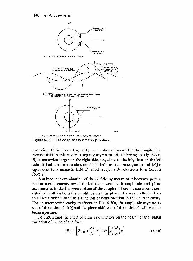
146 G. A. Loew et al.
a ) CROSS-SECTION OF COUPLER CAVITY
ACCELERATING FORCE
b.) FORCE COMPONENTS DUE TO AMPLITUDE AND PHASEASYMMETRY IN THE COUPLER CAVITIES
-OFFSET
C.) COUPLER OFFSET TO CORRECT AMPLITUDE ASYMMETRY
Figure 6-30 The coupler asymmetry problem.
exception. It had been known for a number of years that the longitudinalelectric field in this cavity is slightly asymmetrical. Referring to Fig. 6-30a,Ez is somewhat larger on the right side, i.e., close to the iris, than on the leftside. It had also been understood25'26 that this transverse gradient of \EZ\ isequivalent to a magnetic field By which subjects the electrons to a Lorentzforce Fx.
A subsequent examination of the Ez field by means of microwave pertur-bation measurements revealed that there were both amplitude and phaseasymmetries in the transverse plane of the coupler. These measurements con-sisted of plotting both the amplitude and the phase of a wave reflected by asmall longitudinal bead as a function of bead position in the coupler cavity.For an uncorrected cavity as shown in Fig. 6-30a, the amplitude asymmetrywas of the order of. 10% and the phase shift was of the order of 1.5° over thebeam aperture.
To understand the effect of these asymmetries on the beam, let the spatialvariation of E, be of the form
(6-46)
Design, fabrication, installation, and performance 147
where AE and A0 are the amplitude and phase variations in the jc-directionover the aperture diameter 2a averaged from 0 to d, the cavity length. Then,to first order,
dE (6'47)
From Maxwell's equations, 5 ,̂ and, hence, the Lorentz force Fx are both intime quadrature with dEJdx. Referring to Fig. 6-30b, the deflecting forceF'x, caused by the phase asymmetry and proportional to (A0/2a)£z>0, is inphase with the accelerating force Fz ; it produces a net deflection on a bunchtraveling on the crest of the wave. On the other hand, the force Fx , causedby the amplitude asymmetry and proportional to (l/2d)(AE/EZt0)EZtQ, is inquadrature with the accelerating force Fz; its effect, as shown in an exag-gerated form in Fig. 6-30b, is to spread transversely a bunch traveling on theaccelerating wave crest. In practice, both of these effects occur simultaneouslyand are undesirable.
Using simple electrodynamics, it can be shown that the transverse momen-tum 6px imparted to an electron traveling at an angle 9 with respect to theaccelerating wave crest through a coupler cavity of length d is given by
Spx = eE*'°U \A<f> cos 0 + — sin e] (6-48)4nac I EZ!Q \
This formula is also given in slightly different form in Eq. (7-107).It was shown26 that unless AE/E could be kept smaller than 0.1 % and
A0 less than 0.06°, serious difficulties might arise in steering the beam overthe 2-mile length. In particular, steering of multiple beams of different energiesthrough accelerator sections which are powered for one beam (and hencecause a deflection) and unpowered for another (thus causing no deflection)would have been extremely difficult and probably impossible without pulsedsteering magnets. To remedy these difficulties, several measures were taken.
1 . Offsetting the coupler cavity as shown in Fig. 6-30c almost completelycompensated for the amplitude asymmetry. The value of the offset was foundthrough successive approximations using microwave perturbation measure-ments; for the input cavity it is 0.155 in. and for the output cavity, 0.080 in.Within the accuracy of the measurements, the value of AE/E was therebyreduced to 0.1 % or less.
2. Attempts to compensate for the phase asymmetry inside the couplercavity did not meet with a simple solution. Experiments which intentionallyused slightly misaligned cavities were not successful in reducing A<j>. The onlypractical solution appeared to be a symmetrically fed coupler cavity with twoirises. However, such a solution would have been expensive and fairlyimpractical since it would have required an additional power splitter.
The baba-abab waveguide configuration shown in Fig. 5-17 is actually apractical version of the double iris coupler where the symmetrical feeding is

148 G. A. Loew et a/.
done on successive sections. Of all the alternative configurations, the abba-abba or baab-baab periodicities would have been the simplest because theywould have re-established a parallel and axial beam over a 40-ft length. Inpractice, because of waveguide flange interferences, these configurations couldnot be adopted, and the baba-abab periodicity was chosen. Its only disad-vantage is that over a 40-ft length, a beam entering on axis and parallel to itemerges parallel to the axis but with a net transverse displacement. The next40-ft length produces the reverse effect and brings the beam back on axis.Hence this periodicity would require that klystrons be turned on and off inpairs so that over an 80-ft length the beam always remains on axis. In practice,this measure is never used. The effect is only serious at low energy in the firsttwo or three sectors of the machine.28 When a klystron must be turned off,the resulting steering effect is compensated by the dc magnetic steering dipolesavailable in the drift sections.
3. Although it was not possible to compensate for the phase asymmetry,its effect was reduced by causing the output coupler of a section to cancelpart of the deflection created by the input coupler. Because the phase shift A0appears to be in the direction of power flow, this reduction in net deflectionwas obtained by having the input and output waveguide feeds on the sameside. This remedy did not achieve total cancellation because the values of(A0/2a)in and (A0/2a)out differ by 30 to 40% in the constant-gradientstructure.
6-3 Fabrication, assembly, and installation
Fabrication (ALE)
A number of techniques of fabricating disk-loaded waveguide capable ofmeeting the close tolerances necessary to obtain the correct phase and groupvelocities were explored at Stanford. Of the many methods considered, onlythree were ever used to construct accelerator sections, namely, shrinking,electroforming, and brazing. The shrinking method2 was used at Stanford toconstruct the original 300-ft, 1-GeV accelerator (Mark III), but it was con-sidered unsatisfactory for the SLAC machine when compared to the othertwo techniques.
Extensive work with electroforming and brazing demonstrated thatsatisfactory disk-loaded waveguide sections could be made by either of thesetechniques. The specification for maximum phase shift excursions at any pointalong the axis of a 10-ft section was set to ±2.5°. This corresponds to amechanical tolerance of ±0.00005 in. for 2b; +0.0002 and -0.0000 in. for2a; ±0.001 in. for d; ±0.0002 in. for t; and ±0.0005 in. for p (see Fig. 6-2).It is evident from these tolerances that special techniques had to be utilized ifthey were to be achieved economically.
The most exacting of the tolerances was the ±0.00005 in. required for

Design, fabrication, installation, and performance 149
the 2b dimension. The first step in meeting this requirement consisted ofmachining the parts that went into the assembly to a tolerance of +0.0002and —0.0000 in. It was not sufficient simply to air-condition the room in whichthese parts were made; it was also essential that a temperature-controlledcutting solution be flowed over the parts during the machining operation.Hence, these parts were machined in an air-conditioned room and with acoolant oil, controlled within 0.25°C. After the assembly was completed, theequivalent of the 0.00005-in. tolerance was achieved by making slight defor-mations in the wall of each cavity as discussed briefly earlier in this chapterand described further below. This procedure was feasible with either thebrazing or the electroforming methods of fabrication.
Satisfactory sections were obtained with both the electroforming andbrazing techniques. However, extensive studies indicated that brazing wasthe preferable way of fabricating the 10,000 ft of disk-loaded waveguide. Thedecision to use the brazing technique was based primarily on the higherdegree of flexibility inherent in this method; it required only a few hours tocomplete a brazed assembly, whereas it took 9 days to complete an electro-formed assembly. However, it is significant to note that for the large-scaleproduction required at SLAC, the cost of the electroforming technique wasestimated to be the same as the cost of the brazing technique within the accur-acy of the estimates. For the sake of completeness, descriptions of bothfabrication techniques are included below.
Figure 6-31 shows an exploded view of the parts used for electroforming,together with a completed piece of disk-loaded waveguide made by thisprocess. The first step in the electroforming method of fabrication was theassembly of a 10-ft array consisting of the copper disks and aluminum spacersshown in the figure. After the parts were assembled in a V-block, a mandrelwas inserted through the holes to hold the assembly together. The assembly
Figure 6-31 Exploded view of parts assembled for the electroformingprocess.
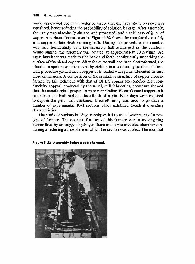
150 G. A. Loew et a/.
work was carried out under water to assure that the hydrostatic pressure wasequalized, hence reducing the probability of solution leakage. After assembly,the array was chemically cleaned and processed, and a thickness of f in. ofcopper was electroformed over it. Figure 6-32 shows the completed assemblyin a copper sulfate electroforming bath. During this procedure, the mandrelwas held horizontally with the assembly half-submerged in the solution.While plating, the assembly was rotated at approximately 30 rev/min. Anagate burnisher was made to ride back and forth, continuously smoothing thesurface of the plated copper. After the outer wall had been electroformed, thealuminum spacers were removed by etching in a sodium hydroxide solution.This procedure yielded an all-copper disk-loaded waveguide fabricated to veryclose dimensions. A comparison of the crystalline structure of copper electro-formed by this technique with that of OFHC copper (oxygen-free high con-ductivity copper) produced by the usual, mill fabricating procedure showedthat the metallurgical properties were very similar. Electroformed copper as itcame from the bath had a surface finish of 6 /zin. Nine days were requiredto deposit the f-in. wall thickness. Electroforming was used to produce anumber of experimental 10-ft sections which exhibited excellent operatingcharacteristics.
The study of various brazing techniques led to the development of a newtype of furnace. The essential features of this furnace were a moving ringburner fired by an oxygen-hydrogen flame and a water-cooled chamber con-taining a reducing atmosphere in which the section was cooled. The essential
Figure 6-32 Assembly being electroformed.

Design, fabrication, installation, and performance 151
Figure 6-33 Schematic view of flame furnace.
features of the flame furnace are illustrated in Fig. 6-33 which shows a 10-ftsection nearing the completion of the brazing cycle. The procedure wascarried out by first stacking the parts in the V-block which is shown at theright. The brazing alloy, which is a silver-copper eutectic melting at 783°C,was inserted at each joint in the form of thin washers. The stacking of theunit parts shown in Fig. 5-12 was carried out while the V-block was at a 75°angle to the vertical. After the stacking was completed, a mandrel wasinserted through the assembly and the end was clamped by a spring-loadedmechanism. The V-block was then tilted to the vertical position, and theentire assembly was moved into the furnace by means of a jib crane. Theupper water-cooled cylinder Was held in the fully raised position, while theassembly was transferred to the furnace and hooked onto a metal tube whichthen served to support it. The disk-loaded section then hung as a free " plumbbob." Any swinging motion was damped by means of the water baffleassembly. After the section was suspended, the split ring burner was closed

152 G. A. Loew et at.
around the disk-loaded waveguide. The burner was then raised to the upper-most end of the disk-loaded waveguide and the oxygen-hydrogen burner wasignited. When the melting point of the brazing alloy was reached, the ringburner together with the upper cylinder was caused to move down the 10-ftsection by means of the two lead screw sets. One lead screw set drove thecylinder, the other drove the ring burner. Oxidation of the interior of thedisk-loaded waveguide section was prevented by flowing a reducing gasthrough the metal tube. Reducing gas also flowed into the upper cylinder,providing a reducing atmosphere for the exterior of the section. A period of25 to 30 min was required from the initiation of the heating cycle to its com-pletion. The section was ready for removal from the furnace 2\ hours afterthe heating cycle was finished.
Figure 6-34 shows the connection of the 10-ft assembly to its supportingtube and the " nose " plate which served as a closure for the cylinder contain-ing the reducing atmosphere in, which the assembly was cooled. Figure 6-35shows the furnace in operation with the flame on.
Input and output waveguide couplers were made up as separate sub-assemblies. Each subassembly consisted of the input or output waveguidecoupler, the end flange, and approximately 8 in. of disk-loaded waveguide.These units were matched in advance as described earlier in this chapter andthen were used in the stacking of a complete 10-ft section. Actually, onceproduction on a large scale had started, the coupler parts were machined so
Figure 6-34 Connection of 10-ft assemblyto support tube.
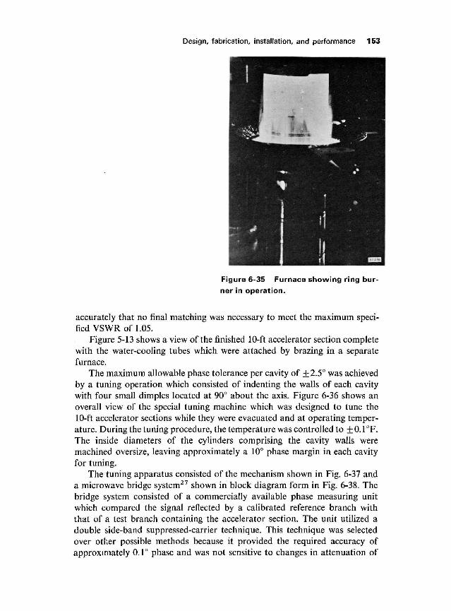
Design, fabrication, installation, and performance 153
Figure 6-35 Furnace showing ring bur-ner in operation.
accurately that no final matching was necessary to meet the maximum speci-fied VSWR of 1.05.
Figure 5-13 shows a view of the finished 10-ft accelerator section completewith the water-cooling tubes which were attached by brazing in a separatefurnace.
The maximum allowable phase tolerance per cavity of +2.5° was achievedby a tuning operation which consisted of indenting the walls of each cavitywith four small dimples located at 90° about the axis. Figure 6-36 shows anoverall view of the special tuning machine which was designed to tune the10-ft accelerator sections while they were evacuated and at operating temper-ature. During the tuning procedure, the temperature was controlled to ±0.1°F.The inside diameters of the cylinders comprising the cavity walls weremachined oversize, leaving approximately a 10° phase margin in each cavityfor tuning.
The tuning apparatus consisted of the mechanism shown in Fig. 6-37 anda microwave bridge system27 shown in block diagram form in Fig. 6-38. Thebridge system consisted of a commercially available phase measuring unitwhich compared the signal reflected by a calibrated reference branch withthat of a test branch containing the accelerator section. The unit utilized adouble side-band suppressed-carrier technique. This technique was selectedover other possible methods because it provided the required accuracy ofapproximately 0.1 ° phase and was not sensitive to changes in attenuation of

154 G. A. Loew et al.
Figure 6-36machine.
Overall view of the tuning
the test signal with respect to the reference signal. Insensitivity to changes inattenuation was important because the amplitude of the wave reflected fromthe shorting plunger changed with the position of the plunger in the accelera-tor section. Furthermore, a unit was required that gave a direct phase readoutso that the operator could monitor and control the amount of tuning requiredfor each cavity. The mechanism by which the actual tuning was accom-plished, illustrated in Fig. 6-37, worked in the following way: the movablecarriage holding the indenters was indexed at the center of each cavity. Con-nected to the movable carriage was the expandable shorting plunger. The rodholding the plunger was coupled and indexed with the movable carriage bymeans of steel tapes. The indentation of the cavities was accomplished bymeans of four hydraulically driven cylinders which pushed the f-in. diameterindenters into the wall of the cavity. The plunger driving rod was made ofInvar to insure dimensional stability in the location of the shorting plunger.Two O-ring seals allowed the rod to move into and out of the evacuatedsection.
The tuning of the section began with the installation of a 10-ft section asshown in Fig. 6-36. The reference arm of the bridge circuit was then calibratedby means of a reference standard which consisted of a precise, movable shortwith three calibrating positions corresponding to the three Smith chart

Design, fabrication, installation, and performance 155
VERTICALSUPPORT
BOO
Figure 6-37 Tuning mechanism showingmovable carriage and indenters.
branches for the 2n/3 disk spacing of the accelerator structure. After cali-bration with the reference branch, the tuning of the individual cavitiesproceeded.
For quality control purposes, additional low-power measurements weremade. Measurements were performed to check the phase of each cavity, the
Figure 6-38 Block diagram of the phasemeasuring system.
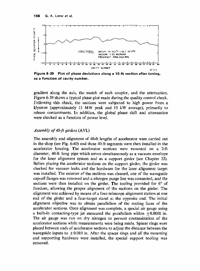
156 G. A. Loew et a/.
CONDITIONS: WATER: IN I I3. I°F-OUT II2.9°FVACUUM: < 25 MICRONSFREQUENCY: 2856.ooo MHZ
i i i i i iO 3 6 9 12 15 IS 21 24 27 30 33 36 39 42 45 48 51 54 57 6O 63 66 69 72 75 78 81 64
CAVITY NUMBER
Figure 6-39 Plot of phase deviations along a 10-ft section after tuning,as a function of cavity number.
gradient along the axis, the match of each coupler, and the attenuation.Figure 6-39 shows a typical phase plot made during the quality control check.Following this check, the sections were subjected to high power from aklystron (approximately 15 MW peak and 15 kW average), primarily torelease contaminants. In addition, the global phase shift and attenuationwere checked as a function of power level.
Assembly of 40-ft girders (AVL)
The assembly and alignment of 40-ft lengths of accelerator were carried outin the shop (see Fig. 6-40) and these 40-ft segments were then installed in theaccelerator housing. The accelerator sections were mounted on a 2-ftdiameter, 40-ft long pipe which serves simultaneously as a vacuum envelopefor the laser alignment system and as a support girder (see Chapter 22).Before placing the accelerator sections on the support girder, the girder waschecked for vacuum leaks and the hardware for the laser alignment targetwas installed. The exterior of the sections was cleaned, one of the waveguidecap-off flanges was removed and a nitrogen purge line was connected, and thesections were then installed on the girder. The tooling provided for 6° offreedom, allowing the proper alignment of the sections on the girder. Thealignment was achieved by means of a four-telescope alignment station at oneend of the girder and a four-target stand at the opposite end. The initialalignment objective was to obtain parallelism of the mating faces of theaccelerator sections. Once alignment was complete, a special air gauge usinga built-in contacting-type jet measured the parallelism within +0.0001 in.The air gauge was run on dry nitrogen to prevent contamination of theaccelerator sections while measurements were being made. Spacer rings wereplaced between ends of accelerator sections to adjust the distance between thewaveguide inputs to +0.010 in. After the spacer rings and all the mountingand supporting hardware were installed, the special support tooling wasremoved.

Design, fabrication, installation, and performance 157
Figure 6-40shop.
View of two finished 40-ft modules in assembly
The vacuum manifold was then installed, and the accelerator sectionswere precisely aligned using the optical tooling holes in the 10-ft acceleratorsection supports. The alignment tolerance allowed only 0.001 in. displace-ment of any accelerator section relative to its adjoining section and a maximumof 0.005 in. total straightness error. Twist had to be avoided since the weldedjoints between 10-ft sections are extremely stiff in torsion, and once the weldwas made, the error could not be removed. After alignment, the jointsbetween 10-ft sections were welded using argon cover gas and nitrogenbacking gas.
At this point, the rectangular waveguide S-assemblies (see Chapter 11)were installed, bolted to the waveguide input, and welded to the vacuummanifold. Then RF loads were added.
Following this installation, the assembly was vacuum tested. Two vacuumtests were performed. The first test consisted of evacuating to approximately10" * torr, connecting a mass spectrometer leak detector to the system, andleak checking by placing helium-filled enclosures about each welded, end-bolted joint. A fine helium probe was used to pinpoint leak locations wherenecessary. Any detected leaks (greater than 10~10 cc/sec) were repaired beforeproceeding. The second vacuum test consisted of measurements of pressureand time required to attain certain pressure levels. In this test, the vacuumwas roughed down to 1 torr, reduced further to 10~4 torr with the liquidnitrogen thimble, and then pumped down with the ion pump. The time re-quired to reach each pressure point was recorded and compared to a standard.

158 G. A. Loew et a/.
The vacuum envelope had to attain 3 x 10"7 torr in less than 8 hours tobe acceptable. Upon completion of the vacuum checks, the acceleratorwas pressurized to 2 psig with dry nitrogen and pinched off.
Several parallel operations were carried out simultaneously with thevacuum tests. These included the connection of all plumbing to the accelera-tor sections, waveguides, and loads, and installation of magnetic shielding,demagnetizing, and degaussing wires. Final alignment was then carried out,and the girder assembly was loaded onto a transporter for the trip to theaccelerator housing. A more detailed description of the girder assemblyoperation can be found in Reference 29.
Installation (AVL)
Completed girder assemblies were transported from the assembly area to theaccelerator housing on a special trailer. The trailer length was adjustable toaccommodate girders of varying lengths (from the 9-ft drift section girder tothe standard 40-ft long girder) by placing girder support frames of variouslengths on a running gear equipped with pneumatic tires. The maximumacceleration of the girder assembly in transit was specified to be 0.3 g. Anaccelerometer was mounted on the girders during transport and the dynamicloading was recorded. The maximum allowable loading of 0.3 g was notexceeded and nearly all girder assemblies were subjected to a dynamic loadingof less than 0.2 g.
The girder assemblies were transported on the special trailer over theroad to the west portal of the accelerator housing and up the aisle in theaccelerator housing to their approximate final location. Two air-film sup-ported pallets were then placed under the girder support frame and therunning gear was removed. The air-film supported pallets allowed the entireassembly to be slipped sideways from the aisle into the beam line and adjustedto the correct position. Figure 6-41 shows a girder being moved from the aisleside of the accelerator housing into the beam line position. The girder wasraised to the correct elevation by means of jacks built into the pallets. Thegirder weight was then transferred to the floor jacks, and the girder supportframe and air-film supported pallets were removed.
After the girders were set in place and roughly aligned, connections weremade to the penetration waveguides. The vacuum manifold was welded tothe vacuum finger and to the vacuum manifold on the adjoining girders, andthe beam line intergirder bellows were welded. When all the girders within^ sector were installed and the vacuum system was completed as describedabove, the entire, sector was evacuated. After evacuation and connection ofthe water-cooling lines to the accelerator sections and waveguide, the wave-guide was phase tuned (see Chapter 11).
Subsequently, the downbeam end of each girder was accurately positionedwith respect to the upbeam end of the following girder in the cross-jointalignment process. This process is described in Chapter 22. Upon completion,
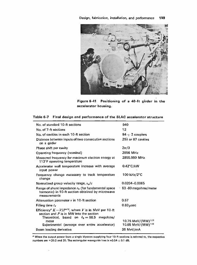
Design, fabrication, installation, and performance 159
Figure 6-41 Positioning of a 40-ft girder in theaccelerator housing.
Table 6-7 Final design and performance of the SLAC accelerator structure
No. of standard 10-ft sections
No. of 7-ft sections
No. of cavities in each 10-ft section
Distance between inputs of two consecutive sectionson a girder
Phase shift per cavity
Operating frequency (nominal)
Measured frequency for maximum electron energy at113°F operating temperature
Accelerator wall temperature increase with averageinput power
Frequency change necessary to track temperaturechange
Normalized group velocity range, vg/c
Range of shunt impedance r0 (for fundamental spaceharmonic) in 10-ft section obtained by microwavemeasurements
Attenuation parameter r in 10-ft section
Filling time tFEfficiency" K = V/P1/2, where V is in MeV per 10-ft
section and P is in MW into the sectionTheoretical, based on F0 = 56.5 megohms/
meterExperimental (average over entire accelerator)
Beam loading derivative
940
12
84 + 2 couplers
29A or 87 cavities
27T/3
2856 MHz
2855.980 MHz
0.42°C/kW
100 kHz/2°C
0.0204-0.0065
53-60 megohms/meter
0.57
0.83 p,sec
10.75MeV/(MW)m
10.65MeV/(MW)l/2
35 MeV/mA
" When the output power from a single klystron supplying four 10-ft sections is referred to, the respectivenumbers are «20.2 and 20. The rectangular waveguide loss is »0.54 ± 0.1 dB.

160 G. A. Loew et a/.
the 2-ft diameter, light pipe bellows were inserted between girders and weldedin place. The welds were made in one sector at a time and the sector was thenchecked for leaks. Next, sectors were joined together and checked for leaksin groups. Finally, the degaussing wires, demagnetizing wires, phase referencecables, and other connections were made.
A more detailed description of the installation process can be found inReference 29.
6-4 Summary of design and performance (GAL)
To conclude this chapter, it seems appropriate to summarize the main per-formance characteristics of the accelerator structure. Of course, the perfor-mance of the accelerator structure cannot be divorced from that of themachine as a whole, and hence, many of the operational results have alreadybeen reported in Chapter 5. In retrospect, it can be said that, so far, the accel-erator structure has lived up to all the expectations and specifications forwhich it was designed. It has failed only in one respect in that the cumulative,multisection-type of beam breakup was not foreseen in advance. This prob-lem continues to be under intensive investigation as this book is being writtenand a detailed up-to-date discussion can be found in Chapter 7. The finaldesign and performance data of the accelerator structure are summarizedin Table 6-7.
Acknowledgments
The authors would like to thank those members of the Stanford LinearAccelerator Center staff who have contributed to the work reported here. Inparticular, they wish to acknowledge the contributions of O. Altenmueller,W. J. Gallagher, B. Kendall, A. Kirshbaum, C. Kruse, J. Abraham, L. Cain,R. Chapton, M. Heinz, D. Jeong, F. Patton, J. A. Pope, C. Rasmussen,D. Robertson, D. Rogers, K. Skarpaas, H. Soderstrom, and B. Stillman.
References
1 E. L. Ginzton, W. W. Hansen, and W. R. Kennedy, Rev. Set. Instr. 19, 89(1948).
2 M. Chodorow et a/., Rev. Sci. Instr. 26, 134 (1955).
3 R. B. Neal, " Theory of the Constant Gradient Linear Electron Accelerator,"Rept. No. ML-513, Microwave Laboratory, Stanford University, Stanford,California (1958); and "Comparison of the Constant Gradient and UniformAccelerator Structures," Rept. No. M-259, Stanford Linear Accelerator Center,Stanford University, Stanford, California (1961).
4 J. E. Leiss and R. A. Schrack, "Transient and Beam Loading Phenomena inLinear Electron Accelerators," Internal Report, Natl. Bur. Standards, Wash-ington, B.C. (October 30, 1962).

Design, fabrication, installation, and performance 161
5 M. G. Kelliher and R. Beadle, Nature 187, 1099 (1960).
6 M. C. Crowley-Milling, T. R. Jarvis, C. W. Miller, and G. Saxon, Nature 191,483 (1961).
7 "Linear Electron Accelerator Studies; Status Rept. 1 October to 31 December,1958," Rept. No. ML-581, Microwave Laboratory, Stanford University,Stanford, California (February 1959).
8 P. B. Wilson, "A Study of Beam-Blow up-in Electron Linacs," Rept. No.HEPL-297, High Energy Physics Laboratory, Stanford University, Stanford,California (June 1963).
9 R. Kingsland, Hughes Aircraft Company, Fullerton, California (private commu-nication).
10 E. L. Ginzton, Microwave Measurement, McGraw-Hill, New York, 1957.
11 W. J. Gallagher, " Measurement Techniques for Periodic Structures," Rept.No. M-205, Stanford Linear Accelerator Center, Stanford University, Stanford,California (November 1960).
12 P. N. Robson, "Fourier Series Representations of Dispersion Curves forCircular Corrugated Waveguide Used in Traveling-Wave Linear Accelerators,"Rept. No. 5105, Metropolitan-Vickers Electrical Company, Ltd., Manchester,England (1956).
13 W. R. Ayers, E. L. Chu, and W. J. Gallagher, " Measurements of InteractionImpedance in Periodic Circuits," Rept. No. ML-403, Microwave Laboratory,Stanford University, Stanford, California (June 1957).
14 "Linear Electron Accelerator Studies and Proposed Two-Mile AcceleratorProject; (combined) Status Report, 1 October to 31 December 1960," Rept.No. M-246, Stanford Linear Accelerator Center, Stanford University, Stanford,California (January 1961).
15 K. B. Mallory, "A source of error in the use of slope detection for perturbationmeasurements," Inst. Radio Engrs. Trans. Microwave Theory Tech., 10, 146(1962).
16 Renee Hirel, " Space-Harmonic Content of the 2-rr/3 Accelerator Structure,"Rept. No. M-270, Stanford Linear Accelerator Center, Stanford University,Stanford, California (1961).
17 G. A. Deschamps, /. Appl. Phys. 24, 1046 (1953).
18 Kenneth Brandt Mallory, "A comparison of the predicted and observed per-formances of a billion-volt electron accelerator," Ph.D. Thesis, Stanford Uni-versity, Stanford, California (1955), p. 68 et seg.
19 R. Belbeoch, "Problemes poses par 1'adaption du coupleur d'entree d'unestructure en guide charge par des iris," Rept. No. LAL-13, Laboratoire deL'accelerateur Lineaire, Orsay, France (1961).
20 R. Kyhl (private communication).
21 E. Westbrook, " Microwave Impedance Matching of Feed Waveguides to theDisk-Loaded Accelerator Structure Operating in the 27T-/3 Mode," Tech. NoteSLAC-TN-63-103, Stanford Linear Accelerator Center, Stanford University,Stanford, California (December 1963).

162 G. A. Loew et a/.
22 R. Borghi and D. Jeong, " Gradient Corrections for the SLAC AcceleratingStructure," Tech. Note SLAC-TN-63-60, Stanford Linear Accelerator Center,Stanford University, Stanford, California (1963).
23 R. B. Neal, "Theory of the Constant Gradient Linear Electron Accelerator,"Rept. No. ML-513, Microwave Laboratory, Stanford University, Stanford,California (1958), p. 4, Eq. (3.6).
24 R. B. Neal, " Comparison of the Constant Gradient and Uniform AcceleratorStructures," Rept. No. M-259, Stanford Linear Accelerator Center, StanfordUniversity, Stanford, California (1961), p. 5, Eq. (7).
25 R. H. Helm, "A Note on Coupler Asymmetries in Long Linear Accelerators,"Rept. No. M-167, Stanford Linear Accelerator Center, Stanford University,Stanford, California (1960).
26 R. H. Helm, "Effects of Stray Magnetic Fields and RF Coupler Asymmetryin the Two-Mile Accelerator with Sector Focusing," Rept. No. SLAC-20,Stanford Linear Accelerator Center, Stanford University, Stanford, California(October 1963).
27 R. Borghi, F. Patton, and M. Heinz, Phase velocity adjustment of the SLACaccelerating structure (private communication).
28 SLAC Staff, " Consolidation of Results of Preliminary Beam Tests with Sectors1 and 2," Rept. No. SLAC-50, Stanford Linear Accelerator Center, StanfordUniversity, Stanford, California (1965).
29 A. Lisin, "Girder Assembly and Installation," Tech. Note SLAC TN-67-17,Stanford Linear Accelerator Center, Stanford University, Stanford, California(May 1967).
![Ba - University of Cretetziritas/papers/segment.pdf · Activ econ tours [3], based on lo cal gradien ts as w ell, ha v e b een in tro duced for trac king deformable mo ving ob jects](https://img.pdfslide.us/doc/110x75/5f1b5d5651a3a04ad3253a57/ba-university-of-crete-tziritaspapers-activ-econ-tours-3-based-on-lo-cal.jpg)


![Scanned with CamScanner · 2020. 6. 20. · Tentukan gradien garis singgung g fCu) +2 d)' dengan f.oordinot L 2 clan 3 . singgurg tí€k dengan Koordinat = C -c2+2C+2 1m +2 J -L-c2+2c+2]](https://img.pdfslide.us/doc/110x75/611fcae6f3e14e57a54c4570/scanned-with-camscanner-2020-6-20-tentukan-gradien-garis-singgung-g-fcu-2.jpg)