Chapter 5

Modelling Tides and Storm Surges

in the Great Australian Bight

5.1 Introduction

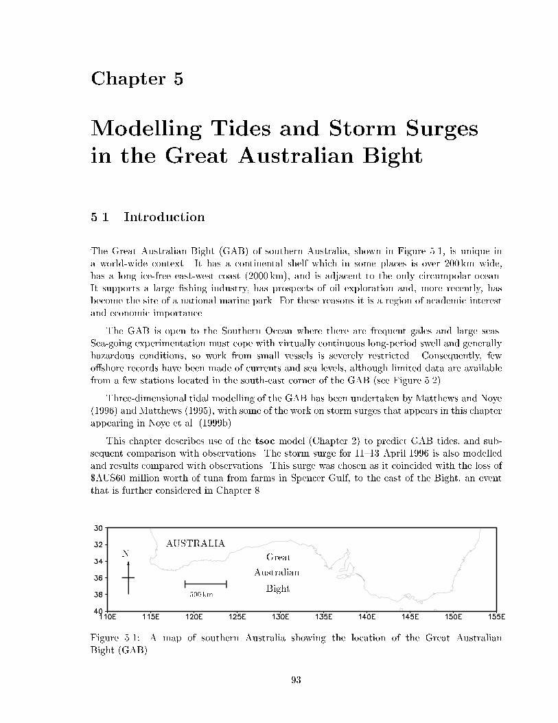
The Great Australian Bight (GAB) of southern Australia, shown in Figure 5.1, is unique ina world-wide context. It has a continental shelf which in some places is over 200 km wide,has a long ice-free east-west coast (2000 km), and is adjacent to the only circumpolar ocean.It supports a large �shing industry, has prospects of oil exploration and, more recently, hasbecome the site of a national marine park. For these reasons it is a region of academic interestand economic importance.

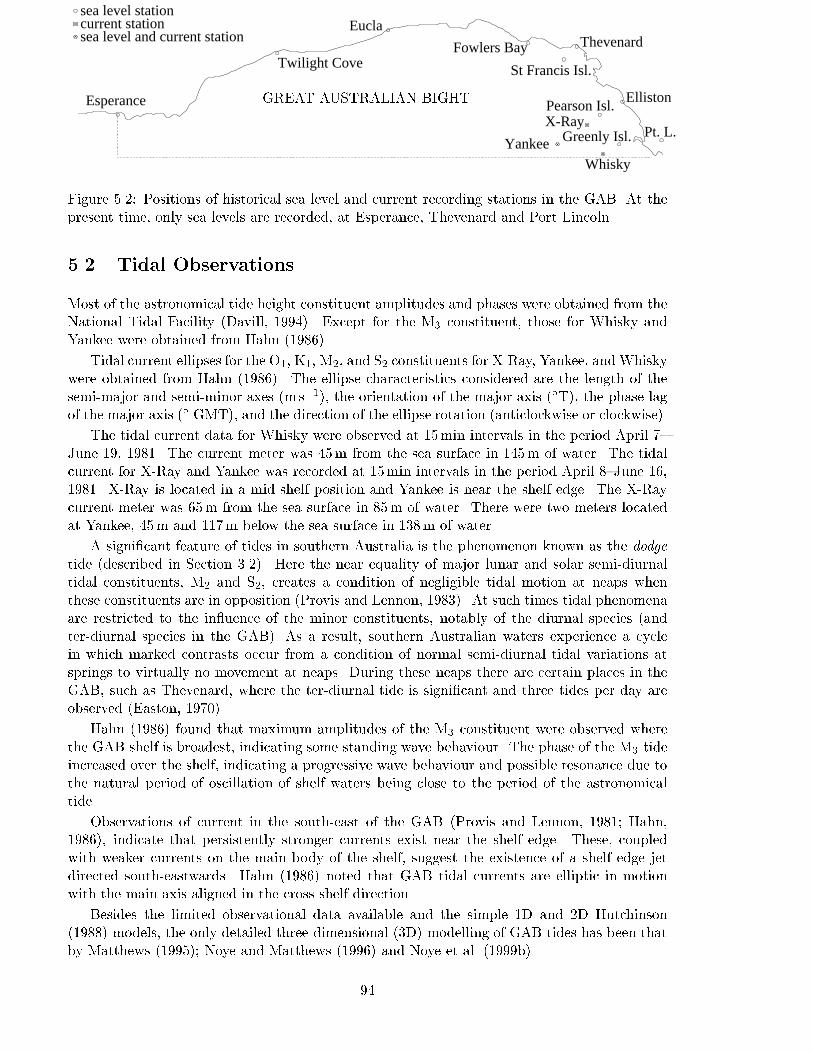
The GAB is open to the Southern Ocean where there are frequent gales and large seas.Sea-going experimentation must cope with virtually continuous long-period swell and generallyhazardous conditions, so work from small vessels is severely restricted. Consequently, fewo�shore records have been made of currents and sea levels, although limited data are availablefrom a few stations located in the south-east corner of the GAB (see Figure 5.2).

Three-dimensional tidal modelling of the GAB has been undertaken by Matthews and Noye(1996) and Matthews (1995), with some of the work on storm surges that appears in this chapterappearing in Noye et al. (1999b).

This chapter describes use of the tsoc model (Chapter 2) to predict GAB tides, and sub-sequent comparison with observations. The storm surge for 11{13 April 1996 is also modelledand results compared with observations. This surge was chosen as it coincided with the loss of$AUS60 million worth of tuna from farms in Spencer Gulf, to the east of the Bight, an eventthat is further considered in Chapter 8.

Great

Australian

Bight

AUSTRALIAN

6

500 km

Figure 5.1: A map of southern Australia showing the location of the Great AustralianBight (GAB).

93

GREAT AUSTRALIAN BIGHTEsperance

Twilight Cove

Eucla

Fowlers Bay

St Francis Isl.

Thevenard

Elliston

Greenly Isl.

Pearson Isl.

sea level station

Pt. L.X-Ray

current station

Yankee

Whisky

sea level and current station

Figure 5.2: Positions of historical sea level and current recording stations in the GAB. At thepresent time, only sea levels are recorded, at Esperance, Thevenard and Port Lincoln.

5.2 Tidal Observations

Most of the astronomical tide height constituent amplitudes and phases were obtained from theNational Tidal Facility (Davill, 1994). Except for the M3 constituent, those for Whisky andYankee were obtained from Hahn (1986).

Tidal current ellipses for the O1, K1, M2, and S2 constituents for X-Ray, Yankee, andWhiskywere obtained from Hahn (1986). The ellipse characteristics considered are the length of thesemi-major and semi-minor axes (m s�1), the orientation of the major axis (�T), the phase lagof the major axis (� GMT), and the direction of the ellipse rotation (anticlockwise or clockwise).

The tidal current data for Whisky were observed at 15min intervals in the period April 7{June 19, 1981. The current meter was 45m from the sea surface in 145m of water. The tidalcurrent for X-Ray and Yankee was recorded at 15min intervals in the period April 8{June 16,1981. X-Ray is located in a mid shelf position and Yankee is near the shelf edge. The X-Raycurrent meter was 65m from the sea surface in 85m of water. There were two meters locatedat Yankee, 45m and 117m below the sea surface in 138m of water.

A signi�cant feature of tides in southern Australia is the phenomenon known as the dodge

tide (described in Section 3.2). Here the near equality of major lunar and solar semi-diurnaltidal constituents, M2 and S2, creates a condition of negligible tidal motion at neaps whenthese constituents are in opposition (Provis and Lennon, 1983). At such times tidal phenomenaare restricted to the in uence of the minor constituents, notably of the diurnal species (andter-diurnal species in the GAB). As a result, southern Australian waters experience a cyclein which marked contrasts occur from a condition of normal semi-diurnal tidal variations atsprings to virtually no movement at neaps. During these neaps there are certain places in theGAB, such as Thevenard, where the ter-diurnal tide is signi�cant and three tides per day areobserved (Easton, 1970).

Hahn (1986) found that maximum amplitudes of the M3 constituent were observed wherethe GAB shelf is broadest, indicating some standing wave behaviour. The phase of the M3 tideincreased over the shelf, indicating a progressive wave behaviour and possible resonance due tothe natural period of oscillation of shelf waters being close to the period of the astronomicaltide.

Observations of current in the south-east of the GAB (Provis and Lennon, 1981; Hahn,1986), indicate that persistently stronger currents exist near the shelf edge. These, coupledwith weaker currents on the main body of the shelf, suggest the existence of a shelf edge jetdirected south-eastwards. Hahn (1986) noted that GAB tidal currents are elliptic in motionwith the main axis aligned in the cross shelf direction.

Besides the limited observational data available and the simple 1D and 2D Hutchinson(1988) models, the only detailed three-dimensional (3D) modelling of GAB tides has been thatby Matthews (1995); Noye and Matthews (1996) and Noye et al. (1999b).

94

5.3 The Model

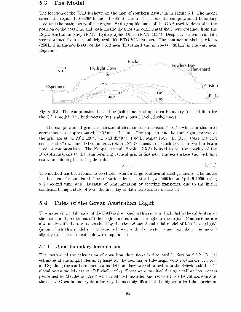
The location of the GAB is shown on the map of southern Australia in Figure 5.1. The modelcovers the region 120�{136� E and 31�{35� S. Figure 5.3 shows the computational boundaryused and the bathymetry of the region. Hydrographic maps of the GAB used to determine theposition of the coastline and bathymetric data for the continental shelf were obtained from theRoyal Australian Navy (RAN) Hydrographic O�ce (RAN, 1995). Deep sea bathymetric datawere obtained from the publicly available ETOPO5 data set. The continental shelf is widest(250 km) in the north-east of the GAB near Thevenard and narrowest (80 km) in the west nearEsperance.

30

200

1000

2000

3000

4000

100 km

Esperance

Twilight Cove

EuclaFowlers Bay

Thevenard

Elliston

Pt. L.

Figure 5.3: The computational coastline (solid line) and open sea boundary (dashed line) forthe GAB model. The bathymetry (m) is also shown (labelled solid lines).

The computational grid has horizontal elements of dimension 50 � 50, which in this areacorresponds to approximately 9.2 km � 7.9 km. The top left and bottom right corners ofthe grid are at 31�200 S 120�500 E and 35�100 S 136� E, respectively. In (�; �) space the gridconsists of 47 rows and 181 columns, a total of 8507 elements, of which less than two thirds areused in computations. The Kappa method (Section 2.5.3) is used to set the spacing of the10 depth intervals so that the resulting vertical grid is �ne near the sea surface and bed, andcoarse at mid depths, using the value

� = 5: (5.3.1)

The method has been found to be stable, even for large continental shelf gradients. The modelhas been run for simulated times of various lengths, starting at 0:00 hr on April 9 1996, usinga 20 second time step. Because of contamination by starting transients, due to the initialcondition being a state of rest, the �rst day of data were always discarded.

5.4 Tides of the Great Australian Bight

The underlying tidal model of the GAB is discussed in this section. Included is the calibration ofthe model and predictions of tide heights and currents throughout the region. Comparisons arealso made with the results obtained by the three-dimensional tidal model of Matthews (1995)(upon which this model of the tides is based, with the western open boundary now movedslightly to the east to coincide with Esperance).

5.4.1 Open boundary formulation

The method of the calculation of open boundary ows is discussed in Section 2.3.2. Initialestimates of the amplitudes and phases for the four major tide-height constituents O1, K1, M2,and S2 along the southern open sea model boundary were obtained from the Schwiderski 1��1�

global ocean model data set (Mitchell, 1994). These were modi�ed during a calibration processperformed by Matthews (1995) which matched modelled and recorded tide-height constants atthe coast. Open boundary data for M3, the most signi�cant of the higher order tidal species at

95

2

4

13

14

1

3

1615

12

. . . . . .

.

.

.

Esperance

177 178176106 107 108 109 110

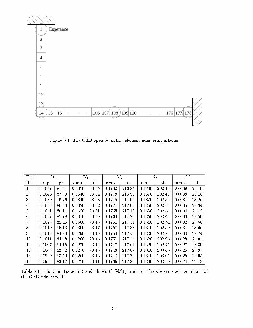
Figure 5.4: The GAB open boundary element numbering scheme.

Bdy O1 K1 M2 S2 M3

Ref. amp. ph. amp. ph. amp. ph. amp. ph. amp. ph.

1 0.1047 87.41 0.1350 93.55 0.1782 216.85 0.1380 202.44 0.0039 28.102 0.1043 87.09 0.1340 93.54 0.1778 216.93 0.1370 202.49 0.0038 28.183 0.1039 86.76 0.1340 93.53 0.1775 217.00 0.1370 202.54 0.0037 28.264 0.1035 86.43 0.1330 93.52 0.1771 217.08 0.1360 202.59 0.0035 28.345 0.1031 86.11 0.1320 93.51 0.1768 217.15 0.1350 202.64 0.0034 28.426 0.1027 85.78 0.1310 93.50 0.1764 217.23 0.1350 202.69 0.0033 28.507 0.1023 85.45 0.1300 93.48 0.1761 217.31 0.1340 202.74 0.0032 28.588 0.1019 85.13 0.1300 93.47 0.1757 217.38 0.1340 202.80 0.0031 28.669 0.1015 84.80 0.1290 93.46 0.1754 217.46 0.1330 202.85 0.0030 28.7410 0.1011 84.48 0.1280 93.45 0.1750 217.54 0.1320 202.90 0.0028 28.8111 0.1007 84.15 0.1270 93.44 0.1747 217.61 0.1320 202.95 0.0027 28.8912 0.1003 83.82 0.1270 93.43 0.1743 217.69 0.1310 203.00 0.0026 28.9713 0.0999 83.50 0.1260 93.42 0.1740 217.76 0.1310 203.05 0.0025 29.0514 0.0995 83.17 0.1250 93.41 0.1736 217.84 0.1300 203.10 0.0024 29.13

Table 5.1: The amplitudes (m) and phases (� GMT) input on the western open boundary ofthe GAB tidal model.

96

Bdy O1 K1 M2 S2 M3

Ref. amp. ph. amp. ph. amp. ph. amp. ph. amp. ph.

14 0.0995 83.17 0.1250 93.41 0.1736 217.84 0.1300 203.10 0.0024 29.1318 0.1015 82.50 0.1280 93.75 0.1741 218.50 0.1310 203.70 0.0024 31.5822 0.1035 81.83 0.1300 94.08 0.1746 219.17 0.1310 204.34 0.0024 33.9026 0.1055 81.17 0.1310 94.41 0.1750 219.84 0.1310 205.11 0.0025 36.2230 0.1075 80.50 0.1330 94.75 0.1748 220.50 0.1310 205.88 0.0025 38.5434 0.1095 79.83 0.1340 95.08 0.1742 221.24 0.1310 206.64 0.0026 40.8638 0.1115 79.17 0.1350 95.41 0.1730 222.20 0.1310 207.39 0.0026 43.1842 0.1135 78.50 0.1370 95.75 0.1719 223.17 0.1310 208.14 0.0026 45.5046 0.1155 77.83 0.1380 96.08 0.1711 224.04 0.1310 208.81 0.0027 47.8250 0.1175 77.17 0.1390 96.41 0.1714 224.61 0.1320 209.24 0.0027 50.1454 0.1195 76.50 0.1410 96.75 0.1717 225.17 0.1320 209.67 0.0028 52.4658 0.1215 75.83 0.1420 97.08 0.1720 225.73 0.1320 210.12 0.0028 54.7862 0.1235 75.17 0.1430 97.41 0.1722 226.27 0.1320 210.58 0.0028 57.1066 0.1255 74.50 0.1450 97.75 0.1724 226.80 0.1320 211.05 0.0029 59.4270 0.1275 73.83 0.1460 98.08 0.1725 227.32 0.1320 211.51 0.0029 63.0074 0.1295 73.17 0.1470 98.41 0.1727 227.80 0.1320 211.94 0.0030 67.0078 0.1320 72.50 0.1490 98.75 0.1729 228.29 0.1320 212.37 0.0030 71.0082 0.1340 71.92 0.1500 99.08 0.1731 228.77 0.1320 212.80 0.0030 75.0086 0.1360 71.58 0.1510 99.41 0.1734 229.23 0.1330 213.22 0.0031 79.0090 0.1380 71.25 0.1530 99.75 0.1737 229.70 0.1330 213.64 0.0031 83.0094 0.1400 70.92 0.1540 100.08 0.1741 230.17 0.1330 214.05 0.0032 87.0098 0.1420 70.58 0.1550 100.41 0.1744 230.63 0.1330 214.47 0.0032 91.00102 0.1440 70.25 0.1570 100.75 0.1747 231.10 0.1330 214.89 0.0032 95.00106 0.1460 69.92 0.1580 101.08 0.1751 231.56 0.1330 215.30 0.0033 99.00110 0.1480 69.58 0.1590 101.41 0.1756 232.01 0.1330 215.70 0.0033 103.00114 0.1500 69.25 0.1610 101.75 0.1761 232.46 0.1330 216.10 0.0034 107.00118 0.1520 69.08 0.1620 102.08 0.1768 232.91 0.1330 216.50 0.0034 111.00122 0.1540 69.42 0.1630 102.41 0.1778 233.34 0.1330 216.86 0.0034 115.00126 0.1560 69.75 0.1650 102.75 0.1788 233.77 0.1330 217.23 0.0035 119.00130 0.1580 70.08 0.1660 103.08 0.1797 234.20 0.1330 217.59 0.0035 123.00134 0.1586 70.42 0.1670 103.41 0.1805 234.58 0.1330 217.96 0.0036 127.00138 0.1592 70.75 0.1690 103.75 0.1814 234.96 0.1330 218.32 0.0036 131.00142 0.1598 71.06 0.1700 104.08 0.1822 235.35 0.1330 218.71 0.0036 135.00146 0.1595 71.30 0.1710 104.41 0.1828 235.73 0.1330 219.14 0.0037 139.00150 0.1589 71.54 0.1730 104.75 0.1835 236.11 0.1330 219.57 0.0037 144.50154 0.1583 71.78 0.1740 105.08 0.1833 236.89 0.1320 220.01 0.0038 150.50158 0.1577 72.02 0.1750 105.41 0.1807 238.84 0.1320 220.45 0.0038 156.50162 0.1571 72.26 0.1770 105.75 0.1780 240.79 0.1320 220.89 0.0038 162.50166 0.1565 72.50 0.1780 106.08 0.1755 242.56 0.1320 221.33 0.0039 168.50170 0.1558 72.74 0.1790 106.41 0.1735 243.81 0.1320 221.77 0.0039 174.50174 0.1552 72.98 0.1800 106.75 0.1715 245.06 0.1320 222.21 0.0040 179.00178 0.1546 73.22 0.1820 107.08 0.1695 246.31 0.1320 222.65 0.0040 183.00

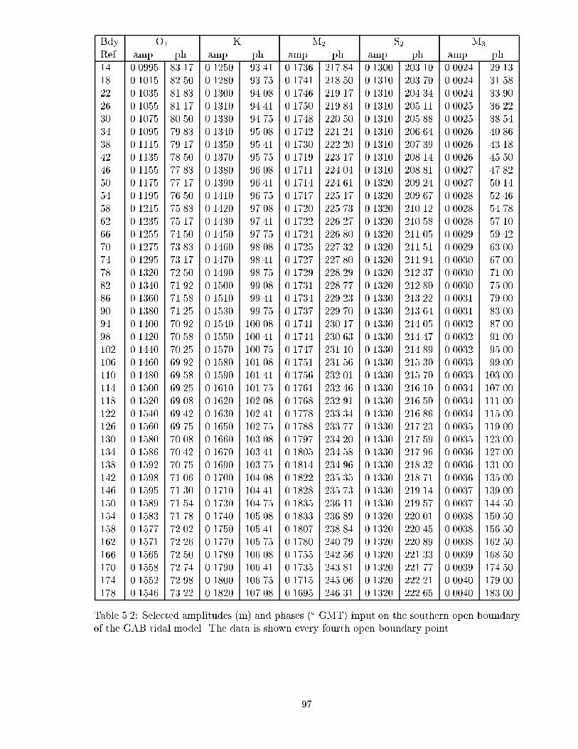
Table 5.2: Selected amplitudes (m) and phases (� GMT) input on the southern open boundaryof the GAB tidal model. The data is shown every fourth open boundary point.

97

Thevenard, were estimated from observations along the coastline. Small amplitudes increasingfrom 0:23 cm in the south-western corner (point 14 in Figure 5.4) to 0:4 cm on the eastern side ofthe GAB (point 178) and phases which increase progressively from 29� in the south-west to 190�

in the east were used for M3 tide-height open boundary data. The tide-height constituents onthe western section of the open boundary (points 1 to 14) were linearly interpolated betweenobservations at Esperance and Schwiderski data at the south-west open boundary gridpoint. Acomplete list of the western boundary constituents is shown in Table 5.1. A list of selected datapoints for the southern boundary is shown in Table 5.2.

5.4.2 Tide height predictions

The model was originally calibrated using an analysis of 29 days of modelled tide heights atstations in the GAB compared with analysed observed data in the form of amplitudes (m) andphases (�). Following Matthews (1995), it was found that the optimal values for the verticaleddy viscosity parameters were

� = 0:0000014m2 s�1; (5.4.2)

� = 0:025:

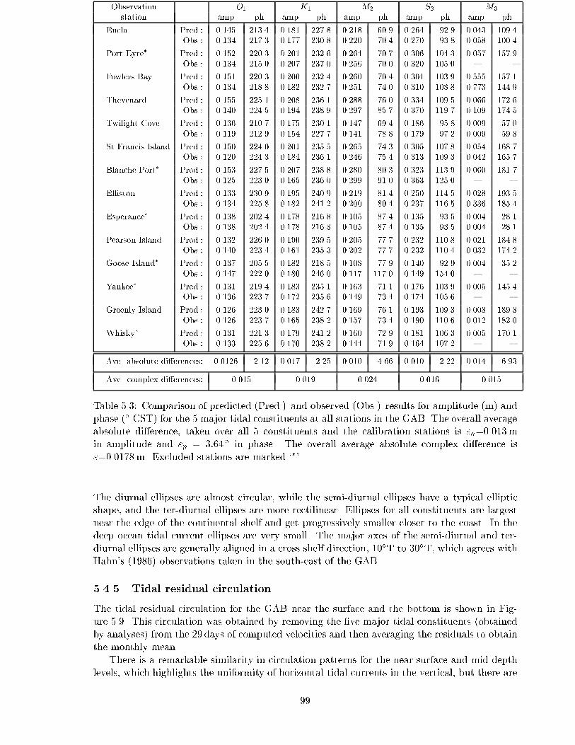
This parameterisation resulted in the predicted amplitudes and phases shown in Table 5.3.

From this table it can be seen that all constituents perform well. The overall complexdi�erence obtained is � = 0:0178m, which is lower than the value obtained by Matthews (1995)in a similar analysis. Note that some stations have been excluded. These are mainly stationswhere an analysis for only four tidal constituents has been made available, with one notableexception. Esperance has been excluded from analysis due to it being an open boundary point.This means that the values at that point should be identical to the tide prescribed there, whichis the case in the table. Use of this point will bias the overall error result.

5.4.3 Modelled co-amplitudes and co-phase diagrams

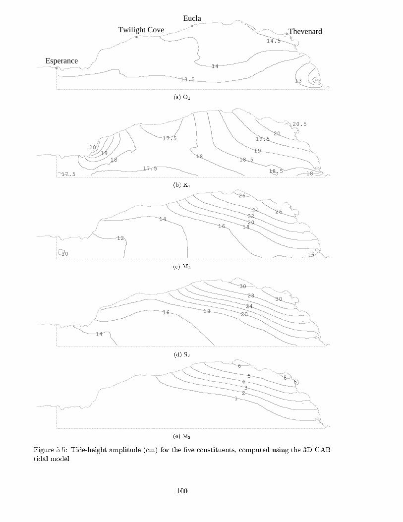
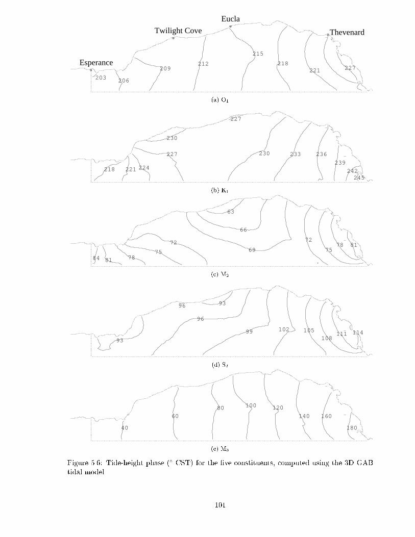
The contours presented in Figures 5.5 and 5.6 show lines of constant tide-height amplitude (cm)and phase (� CST), respectively, for the diurnal constituents O1 and K1, the semi-diurnalconstituents M2 and S2, and the ter-diurnal constituent M3.

Model predictions agree well with observations (Davill, 1994; Hahn, 1986). There is am-pli�cation of the semi-diurnal and ter-diurnal tide-height constituents on the wide continentalshelf near Thevenard and phases generally increase from west to east. A perturbation of theco-amplitude and co-phase lines can be observed for all constituents along the edge of thecontinental shelf, due to the in uence of this feature on the tides.

It is worthy of note that M3 has only 6% of the amplitude of the M2 tide at the shelf edge,but this increases to 25% at the coast near Thevenard.

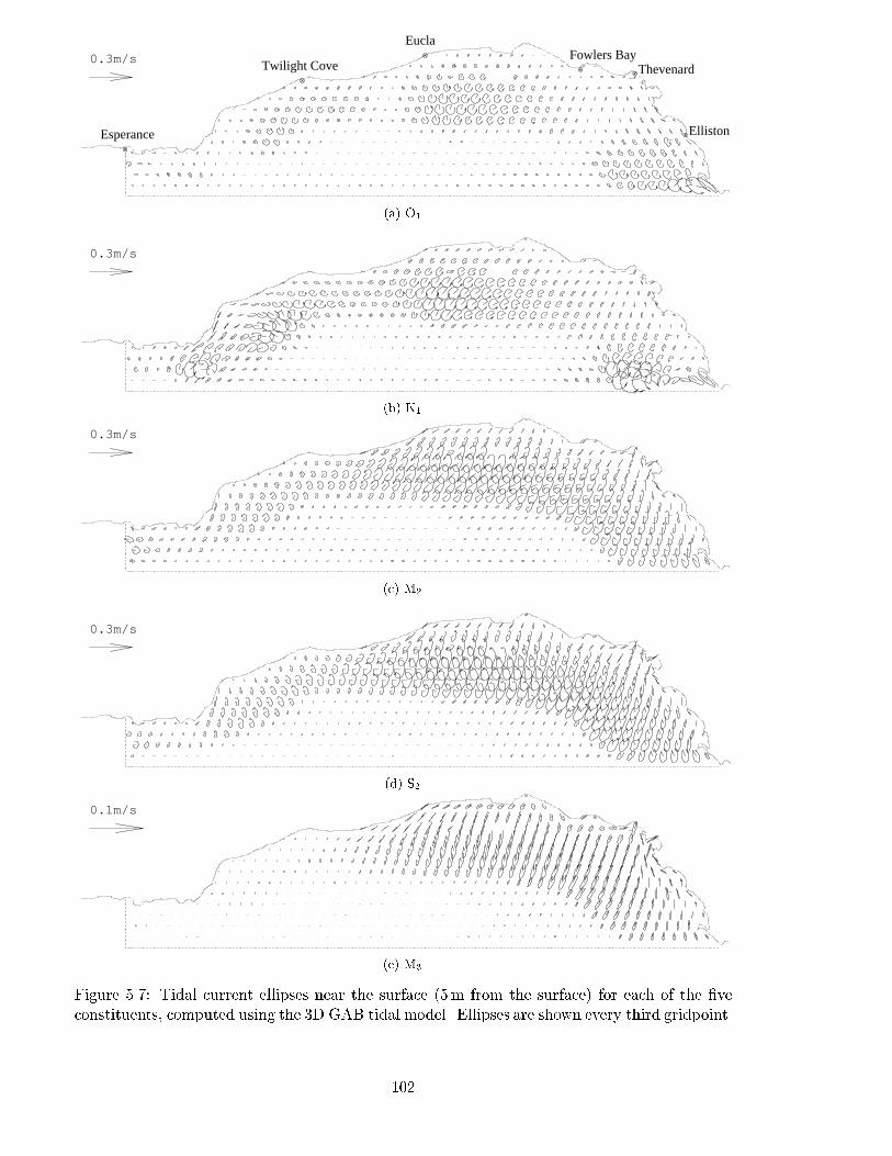
5.4.4 Tidal current ellipses

Depth-dependent predictions for current ellipses near the sea surface (5m below it, obtainedby interpolation) and at mid-depth are approximately the same, but at greater depths theirmagnitude is reduced (see Figures 5.7 and 5.8). For example, the length of the major axis ofthe M2 ellipses 5m above the sea oor are half that near the surface. The biggest di�erencebetween the near surface and near bottom ellipses is in the south-east of the Bight. Ellipses ofstrength comparable to the middle of the GAB can be seen at the surface, but the correspondingbottom ellipses are almost negligible. These di�erences are probably due to the e�ects of bottomfriction.

There is generally an anticlockwise rotation of the tidal current ellipses which agrees withobservations in the south-east of the GAB (Hahn, 1986). However, near the coast from the headof the GAB through to Thevenard clockwise rotating ellipses are predicted for some constituents.

98

Observation O1 K1 M2 S2 M3

station amp ph amp ph amp ph amp ph amp ph

Eucla Pred.: 0.145 213.4 0.181 227.8 0.218 60.9 0.264 92.9 0.043 109.4Obs.: 0.134 217.3 0.177 230.8 0.220 70.4 0.270 93.8 0.058 100.4

Port Eyre� Pred.: 0.152 220.3 0.201 232.6 0.264 70.7 0.306 104.3 0.057 157.9Obs.: 0.134 215.0 0.207 237.0 0.256 70.0 0.320 105.0 { {

Fowlers Bay Pred.: 0.151 220.3 0.200 232.4 0.260 70.4 0.301 103.9 0.555 157.1Obs.: 0.134 218.8 0.182 232.7 0.251 74.0 0.310 103.8 0.773 144.9

Thevenard Pred.: 0.155 225.1 0.208 236.1 0.288 76.0 0.334 109.5 0.066 172.6Obs.: 0.140 224.5 0.194 238.9 0.297 85.7 0.370 119.7 0.109 174.5

Twilight Cove Pred.: 0.136 210.7 0.175 230.1 0.147 69.4 0.186 95.8 0.009 57.0Obs.: 0.119 212.9 0.154 227.7 0.141 78.8 0.179 97.2 0.009 59.8

St Francis Island Pred.: 0.150 224.0 0.201 235.5 0.265 74.3 0.305 107.8 0.054 168.7Obs.: 0.120 224.3 0.184 236.1 0.246 75.4 0.313 109.3 0.042 165.7

Blanche Port� Pred.: 0.153 227.5 0.207 238.8 0.280 80.3 0.323 113.9 0.060 181.7Obs.: 0.125 223.0 0.165 236.0 0.299 91.0 0.363 125.0 { {

Elliston Pred.: 0.133 230.9 0.195 240.9 0.219 81.4 0.250 114.5 0.028 193.5Obs.: 0.134 225.8 0.182 241.2 0.200 80.4 0.237 116.5 0.336 185.4

Esperance� Pred.: 0.138 202.4 0.178 216.8 0.105 87.4 0.135 93.5 0.004 28.1Obs.: 0.138 202.4 0.178 216.8 0.105 87.4 0.135 93.5 0.004 28.1

Pearson Island Pred.: 0.132 226.0 0.190 239.5 0.205 77.7 0.232 110.8 0.021 184.8Obs.: 0.140 223.4 0.161 235.3 0.202 77.7 0.232 110.4 0.032 174.2

Goose Island� Pred.: 0.137 205.5 0.182 218.5 0.108 77.9 0.140 92.9 0.004 35.2Obs.: 0.147 222.0 0.180 246.0 0.117 117.0 0.149 154.0 { {

Yankee� Pred.: 0.131 219.4 0.183 235.1 0.163 71.1 0.176 103.9 0.005 145.4Obs.: 0.136 223.7 0.172 235.6 0.149 73.4 0.174 105.6 { {

Greenly Island Pred.: 0.126 223.0 0.183 242.7 0.169 76.1 0.193 109.3 0.008 189.8Obs.: 0.126 223.7 0.165 238.2 0.157 73.4 0.190 110.6 0.012 182.0

Whisky� Pred.: 0.131 221.3 0.179 241.2 0.160 72.9 0.181 106.3 0.005 170.1Obs.: 0.133 225.6 0.170 238.2 0.144 71.9 0.164 107.2 { {

Ave. absolute di�erences: 0.0126 2.12 0.017 2.25 0.010 4.66 0.010 2.22 0.014 6.93

Ave. complex di�erences: 0.015 0.019 0.024 0.016 0.015

Table 5.3: Comparison of predicted (Pred.) and observed (Obs.) results for amplitude (m) andphase (� CST) for the 5 major tidal constituents at all stations in the GAB. The overall averageabsolute di�erence, taken over all 5 constituents and the calibration stations is "a=0.013min amplitude and "p = 3:64 � in phase. The overall average absolute complex di�erence is"=0.0178m. Excluded stations are marked `�'.

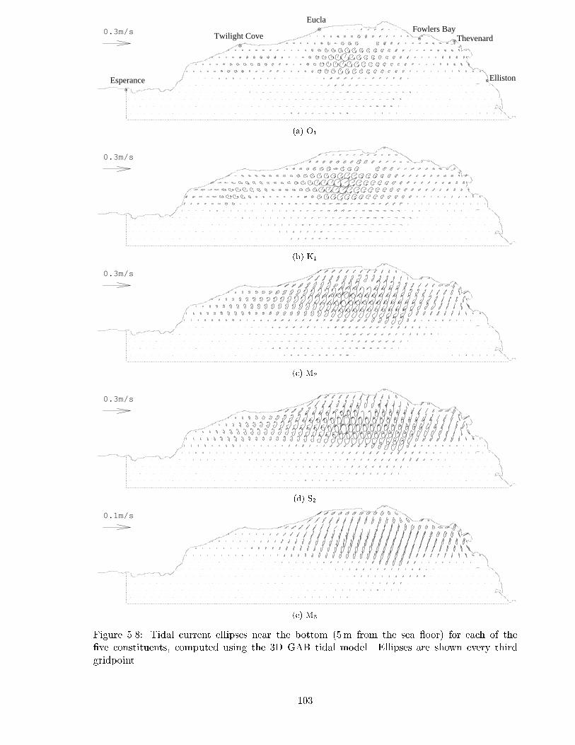
The diurnal ellipses are almost circular, while the semi-diurnal ellipses have a typical ellipticshape, and the ter-diurnal ellipses are more rectilinear. Ellipses for all constituents are largestnear the edge of the continental shelf and get progressively smaller closer to the coast. In thedeep ocean tidal current ellipses are very small. The major axes of the semi-diurnal and ter-diurnal ellipses are generally aligned in a cross shelf direction, 10�T to 30�T, which agrees withHahn's (1986) observations taken in the south-east of the GAB.

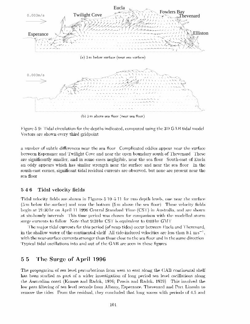
5.4.5 Tidal residual circulation

The tidal residual circulation for the GAB near the surface and the bottom is shown in Fig-ure 5.9. This circulation was obtained by removing the �ve major tidal constituents (obtainedby analyses) from the 29 days of computed velocities and then averaging the residuals to obtainthe monthly mean.

There is a remarkable similarity in circulation patterns for the near-surface and mid-depthlevels, which highlights the uniformity of horizontal tidal currents in the vertical, but there are

99

Esperance

Twilight Cove

Eucla

Thevenard

13.5

14

14.5

13

(a) O1

17.5

1819

20

17.5

18

17.5

18.5

18

19

19.520

20.5

18.5

(b) K1

10

12

1416

16

18202224 26

26

(c) M2

14

16 20

24

2830

30

18

(d) S2

12345

66

6

(e) M3

Figure 5.5: Tide-height amplitude (cm) for the �ve constituents, computed using the 3D GABtidal model.

100

Esperance

Twilight Cove

Eucla

Thevenard

203 206

209212

215

218221 227

(a) O1

218 221 224

227

230

227

230 233 236

239

242245

(b) K1

69

66

63

84 81 7875

72 728178

75

(c) M2

93

96 93

96

99 102 105 114111108

(d) S2

40

60

80 100 120

140 160

180

(e) M3

Figure 5.6: Tide-height phase (� CST) for the �ve constituents, computed using the 3D GABtidal model.

101

Esperance

Twilight Cove

EuclaFowlers Bay

Thevenard

Elliston

0.3m/s

(a) O1

0.3m/s

(b) K1

0.3m/s

(c) M2

0.3m/s

(d) S2

0.1m/s

(e) M3

Figure 5.7: Tidal current ellipses near the surface (5m from the surface) for each of the �veconstituents, computed using the 3D GAB tidal model. Ellipses are shown every third gridpoint.

102

Esperance

Twilight Cove

EuclaFowlers Bay

Thevenard

Elliston

0.3m/s

(a) O1

0.3m/s

(b) K1

0.3m/s

(c) M2

0.3m/s

(d) S2

0.1m/s

(e) M3

Figure 5.8: Tidal current ellipses near the bottom (5m from the sea oor) for each of the�ve constituents, computed using the 3D GAB tidal model. Ellipses are shown every thirdgridpoint.

103

Esperance

Twilight Cove

EuclaFowlers Bay

Thevenard

Elliston

0.003m/s

(a) 5m below surface (near sea surface)

0.003m/s

(b) 5m above sea oor (near sea oor)

Figure 5.9: Tidal circulation for the depths indicated, computed using the 3D GAB tidal model.Vectors are shown every third gridpoint.

a number of subtle di�erences near the sea oor. Complicated eddies appear near the surfacebetween Esperance and Twilight Cove and near the open boundary south of Thevenard. Theseare signi�cantly smaller, and in some cases negligible, near the sea oor. South-east of Euclaan eddy appears which has similar strength near the surface and near the sea oor. In thesouth-east corner, signi�cant tidal residual currents are observed, but none are present near thesea oor.

5.4.6 Tidal velocity �elds

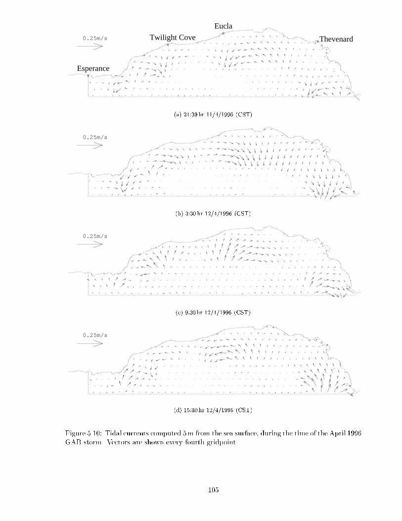
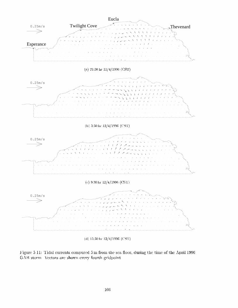
Tidal velocity �elds are shown in Figures 5.10{5.11 for two depth levels, one near the surface(5m below the surface) and near the bottom (5m above the sea oor). These velocity �eldsbegin at 21:30 hr on April 11 1996 Central Standard Time (CST) in Australia, and are shownat six-hourly intervals. This time period was chosen for comparison with the modelled stormsurge currents to follow. Note that 9:30 hr CST is equivalent to 0:00 hr GMT.

The major tidal currents for this period (of neap tides) occur between Eucla and Thevenard,in the shallow water of the continental shelf. All tide-induced velocities are less than 0:1 m s�1,with the near-surface currents stronger than those close to the sea oor and in the same direction.Typical tidal oscillations into and out of the GAB are seen in these �gures.

5.5 The Surge of April 1996

The propagation of sea level perturbations from west to east along the GAB continental shelfhas been studied as part of a wider investigation of long period sea level oscillations alongthe Australian coast (Krause and Radok, 1976; Provis and Radok, 1979). This involved thelow-pass �ltering of sea level records from Albany, Esperance, Thevenard and Port Lincoln toremove the tides. From the residual, they concluded that long waves with periods of 4:5 and

104

Esperance

Twilight Cove

Eucla

Thevenard0.25m/s

(a) 21:30 hr 11/4/1996 (CST)

0.25m/s

(b) 3:30 hr 12/4/1996 (CST)

0.25m/s

(c) 9:30 hr 12/4/1996 (CST)

0.25m/s

(d) 15:30 hr 12/4/1996 (CST)

Figure 5.10: Tidal currents computed 5m from the sea surface, during the time of the April 1996GAB storm. Vectors are shown every fourth gridpoint.

105

Esperance

Twilight Cove

Eucla

Thevenard0.25m/s

(a) 21:30 hr 11/4/1996 (CST)

0.25m/s

(b) 3:30 hr 12/4/1996 (CST)

0.25m/s

(c) 9:30 hr 12/4/1996 (CST)

0.25m/s

(d) 15:30 hr 12/4/1996 (CST)

Figure 5.11: Tidal currents computed 5m from the sea oor, during the time of the April 1996GAB storm. Vectors are shown every fourth gridpoint.

106

9:5 days travelled west to east across the GAB. These waves have much larger amplitudes thansimilar ones observed along the coast of Oregon (Cutchin and Smith, 1973).

Using low-pass �ltered hourly coastal sea level data and atmospheric pressures sampledonce or twice per day, Church and Freeland (1987) carried out a regression of sea levels onatmospheric pressure for Esperance, Thevenard and Port Lincoln. They found an over-responseof sea-level changes to atmospheric pressure variations, relative to the inverse barometric e�ect,and concluded that the large variances obtained indicated that the GAB shelf waters responddynamically to passing weather systems.

In this section, a 3D numerical tide and storm surge model is used to compute the transientlong wave response of the GAB waters to the tides of the Southern Ocean and the rapidlychanging atmospheric pressures and wind stresses during the storm of 11{13 April 1996, a timescale of only 3 days. The results are used to determine whether the large surge which travelledfrom west to east along the coast was caused by weather e�ects or by a free wave moving acrossthe GAB. In this work the surge is the residual obtained by removing the predicted tide-heightfrom the sea level records.

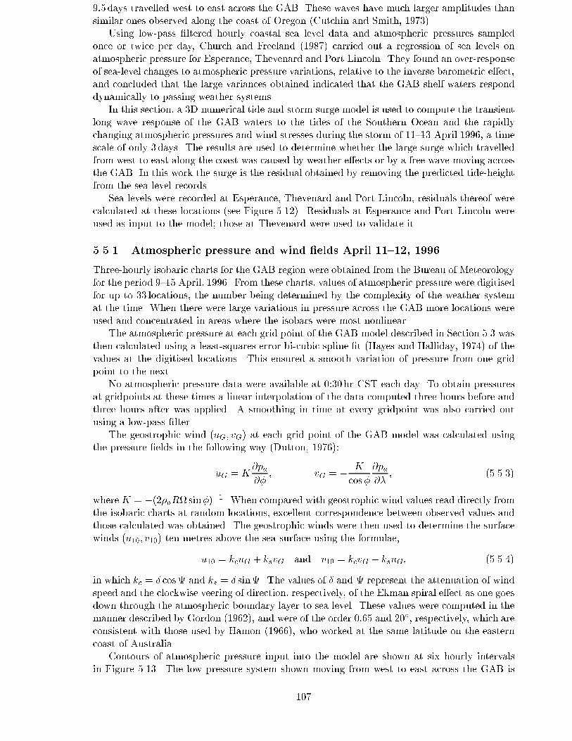
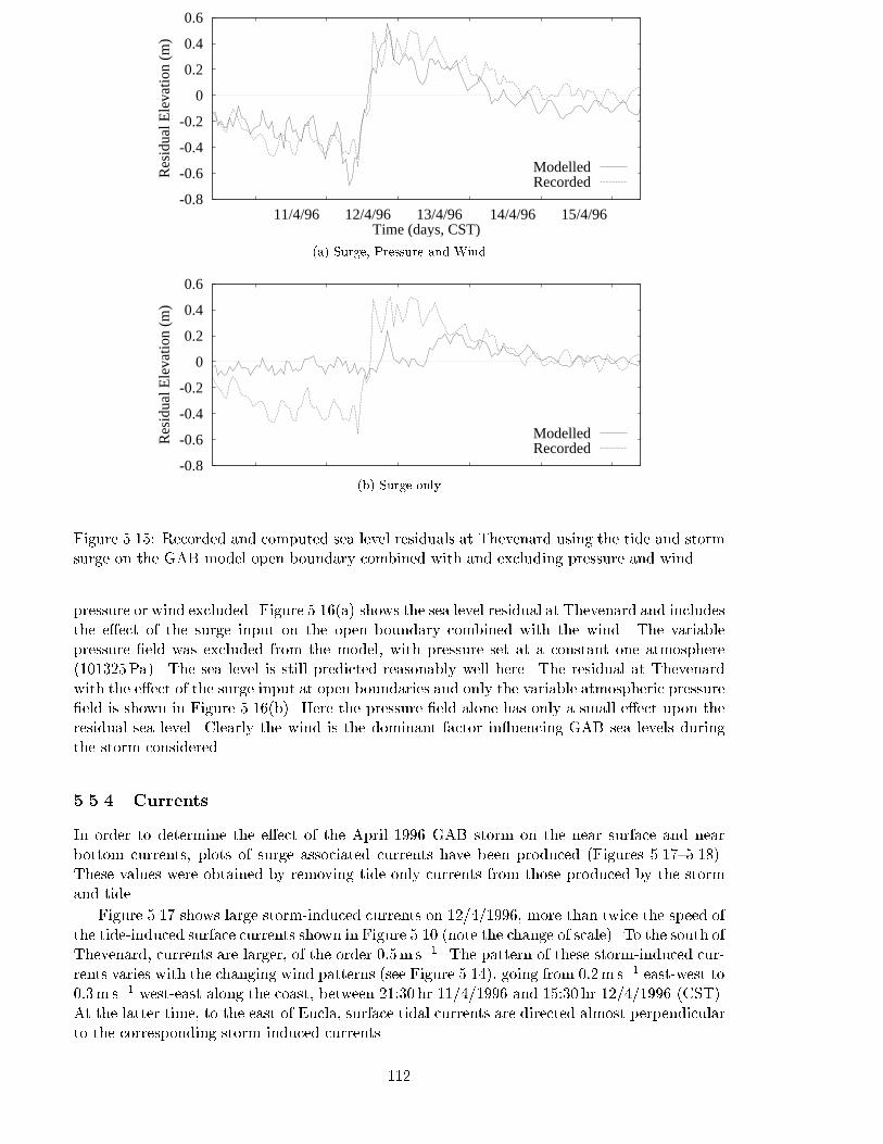
Sea levels were recorded at Esperance, Thevenard and Port Lincoln, residuals thereof werecalculated at these locations (see Figure 5.12). Residuals at Esperance and Port Lincoln wereused as input to the model; those at Thevenard were used to validate it.

5.5.1 Atmospheric pressure and wind �elds April 11{12, 1996

Three-hourly isobaric charts for the GAB region were obtained from the Bureau of Meteorologyfor the period 9{15 April, 1996. From these charts, values of atmospheric pressure were digitisedfor up to 33 locations, the number being determined by the complexity of the weather systemat the time. When there were large variations in pressure across the GAB more locations wereused and concentrated in areas where the isobars were most nonlinear.

The atmospheric pressure at each grid point of the GAB model described in Section 5.3 wasthen calculated using a least-squares error bi-cubic spline �t (Hayes and Halliday, 1974) of thevalues at the digitised locations. This ensured a smooth variation of pressure from one gridpoint to the next.

No atmospheric pressure data were available at 0:30 hr CST each day. To obtain pressuresat gridpoints at these times a linear interpolation of the data computed three hours before andthree hours after was applied. A smoothing in time at every gridpoint was also carried outusing a low-pass �lter.

The geostrophic wind (uG; vG) at each grid point of the GAB model was calculated usingthe pressure �elds in the following way (Dutton, 1976):

uG = K@pa

@�; vG = �

K

cos�

@pa

@�; (5.5.3)

where K = �(2�aRsin�)�1. When compared with geostrophic wind values read directly fromthe isobaric charts at random locations, excellent correspondence between observed values andthose calculated was obtained. The geostrophic winds were then used to determine the surfacewinds (u10; v10) ten metres above the sea surface using the formulae,

u10 = kcuG + ksvG and v10 = kcvG � ksuG; (5.5.4)

in which kc = � cos and ks = � sin. The values of � and represent the attenuation of windspeed and the clockwise veering of direction, respectively, of the Ekman spiral e�ect as one goesdown through the atmospheric boundary layer to sea level. These values were computed in themanner described by Gordon (1962), and were of the order 0:65 and 20�, respectively, which areconsistent with those used by Hamon (1966), who worked at the same latitude on the easterncoast of Australia.

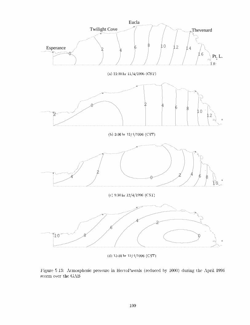
Contours of atmospheric pressure input into the model are shown at six hourly intervalsin Figure 5.13. The low pressure system shown moving from west to east across the GAB is

107

-0.6

-0.4

-0.2

0

0.2

0.4

0.6

0.8

Res

idua

l Ele

vatio

n(m

)

(a) Esperance (smoothed)

-0.6

-0.4

-0.2

0

0.2

0.4

0.6

0.8

Res

idua

l Ele

vatio

n (m

)

(b) Thevenard (unsmoothed)

-0.6

-0.4

-0.2

0

0.2

0.4

0.6

0.8

10/4/96 11/4/96 12/4/96 13/4/96 14/4/96 15/4/96

Res

idua

l Ele

vatio

n (m

)

Time (days, CST)(c) Port Lincoln (smoothed)

Figure 5.12: Hourly observed sea level residual (m) for the period 10/4/1996 to 15/4/1996 (CST)at Esperance, Thevenard and Port Lincoln.

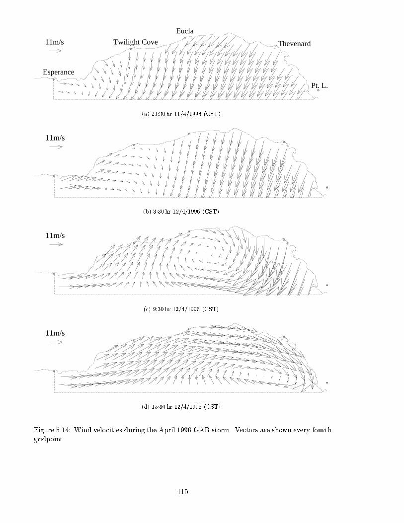
the remnants of Tropical Cyclone OLIVIA. This system (1000HPa), which characterises thestorm, entered from the west below Esperance at 21:30 hr 11/4/1996 (CST), see Figure 5.13(a).Figure 5.14(a) shows that winds at this time were � 13m s�1 and predominantly from the NNEin the eastern and central GAB, from the NNW west of Twilight Cove, and from the W belowEsperance.

At 3:30 hr 12/4/1996 in Figure 5.13(b) the pressure system had moved eastward into theGAB to the south of Twilight Cove, with appropriate changes of wind speed and direction asshown in Figure 5.14(b).

In the following six hours, the system moved along the continental shelf to the region southof Eucla, see Figure 5.13(c). The closeness of adjacent isobars near Thevenard at this timeindicate that the winds associated with the storm were stronger, as con�rmed in Figure 5.14(c),reaching 24m s�1.

By 15:30 hr 12/4/1996 the centre of the storm had reached the south-east corner of theGAB (Figure 5.13(d)). The most signi�cant feature here is the changing of wind direction close

108

Esperance

Twilight Cove

Eucla

Thevenard

Pt. L.02 4

6 8 10 12 1416

18

(a) 21:30 hr 11/4/1996 (CST)

0 2 4 6 810

122

(b) 3:30 hr 12/4/1996 (CST)

42

0 2 4 6 810

(c) 9:30 hr 12/4/1996 (CST)

8

6

10

4 2

0

(d) 15:30 hr 12/4/1996 (CST)

Figure 5.13: Atmospheric pressure in HectoPascals (reduced by 1000) during the April 1996storm over the GAB.

109

Esperance

Twilight Cove

Eucla

Thevenard

Pt. L.

11m/s

(a) 21:30 hr 11/4/1996 (CST)

11m/s

(b) 3:30 hr 12/4/1996 (CST)

11m/s

(c) 9:30 hr 12/4/1996 (CST)

11m/s

(d) 15:30 hr 12/4/1996 (CST)

Figure 5.14: Wind velocities during the April 1996 GAB storm. Vectors are shown every fourthgridpoint.

110

to Thevenard (Figure 5.14(d)). The major surge at Thevenard began to occur about 15:00 hron 12/4/1996 (Figure 5.12), which coincided with the change in wind direction in this six hourperiod.

5.5.2 Modelling the coastal surge

The open boundary conditions of the GAB tidal model were modi�ed in order to simulate thepassage of the storm in addition to the normal tidal oscillation, which is included so that non-linear e�ects are present in the prediction. To do this, the boundary was considered in threesections. The �rst is the deepest part of the open boundary, the south-western section. Thisincludes the western half of the southern open boundary. The wind e�ect on elevation in thisregion was considered negligible due to the deep water involved, and the inverse barometricpressure e�ect (see Section 2.3.2) was applied without modi�cation.

The western and the south-eastern sections of the open boundary were treated di�erentlybecause both cross the continental shelf. In shallow water the inverse barometric pressure e�ectis not an accurate approximation for sea-level change due to the possibility of large wind e�ects.At the coastal end of the western open boundary it was assumed that the sea level behaved asobserved at Esperance. At the coastal end of the southern open boundary, no sea level datawere available. However, data were available from Port Lincoln, a small distance outside themodel domain. The time taken for a surge to travel from the far east open boundary pointto Port Lincoln is approximately three hours. In order to simulate the surge input at the fareast open boundary point, the Port Lincoln observations were smoothed and applied with athree hour lead in time. The surge values between the two open coastal boundary points andthose due to the inverse barometric pressure e�ect in the deep water were determined by linearinterpolation.

5.5.3 Comparison of modelled and recorded surge

The model was run for two days from an initial condition of zero wind and surface pressureof one atmosphere (101325 Pa), gradually changing over the two days to the values of the realwind and pressure data at 9:30 hr on 10/4/1996 CST. The open boundary values were input atrelevant times. All data was interpolated in time so that input �elds were made available everytime step. The model then ran for a further day until 9:30 hr 11/4/1996, to permit the decayof initial transients to a negligible level. Hourly elevations were then stored.

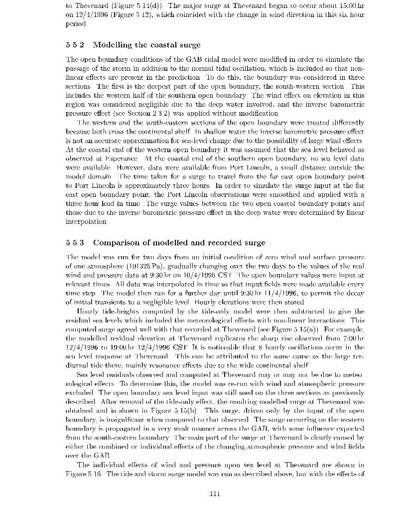
Hourly tide-heights computed by the tide-only model were then subtracted to give theresidual sea levels which included the meteorological e�ects with non-linear interactions. Thiscomputed surge agreed well with that recorded at Thevenard (see Figure 5.15(a)). For example,the modelled residual elevation at Thevenard replicates the sharp rise observed from 7:00 hr12/4/1996 to 19:00 hr 12/4/1996 CST. It is noticeable that 8 hourly oscillations occur in thesea level response at Thevenard. This can be attributed to the same cause as the large ter-diurnal tide there, mainly resonance e�ects due to the wide continental shelf.

Sea level residuals observed and computed at Thevenard may or may not be due to meteo-rological e�ects. To determine this, the model was re-run with wind and atmospheric pressureexcluded. The open boundary sea level input was still used on the three sections as previouslydescribed. After removal of the tide-only e�ect, the resulting modelled surge at Thevenard wasobtained and is shown in Figure 5.15(b). This surge, driven only by the input of the openboundary, is insigni�cant when compared to that observed. The surge occurring on the westernboundary is propagated in a very weak manner across the GAB, with some in uence expectedfrom the south-eastern boundary. The main part of the surge at Thevenard is clearly caused byeither the combined or individual e�ects of the changing atmospheric pressure and wind �eldsover the GAB.

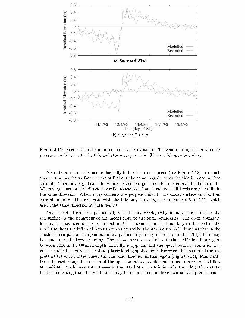
The individual e�ects of wind and pressure upon sea level at Thevenard are shown inFigure 5.16. The tide and storm surge model was run as described above, but with the e�ects of

111

-0.8

-0.6

-0.4

-0.2

0

0.2

0.4

0.6

11/4/96 12/4/96 13/4/96 14/4/96 15/4/96

Res

idua

l Ele

vatio

n (m

)

Time (days, CST)

ModelledRecorded

(a) Surge, Pressure and Wind

-0.8

-0.6

-0.4

-0.2

0

0.2

0.4

0.6

Res

idua

l Ele

vatio

n (m

)

ModelledRecorded

(b) Surge only

Figure 5.15: Recorded and computed sea level residuals at Thevenard using the tide and stormsurge on the GAB model open boundary combined with and excluding pressure and wind.

pressure or wind excluded. Figure 5.16(a) shows the sea level residual at Thevenard and includesthe e�ect of the surge input on the open boundary combined with the wind. The variablepressure �eld was excluded from the model, with pressure set at a constant one atmosphere(101325Pa). The sea level is still predicted reasonably well here. The residual at Thevenardwith the e�ect of the surge input at open boundaries and only the variable atmospheric pressure�eld is shown in Figure 5.16(b). Here the pressure �eld alone has only a small e�ect upon theresidual sea level. Clearly the wind is the dominant factor in uencing GAB sea levels duringthe storm considered.

5.5.4 Currents

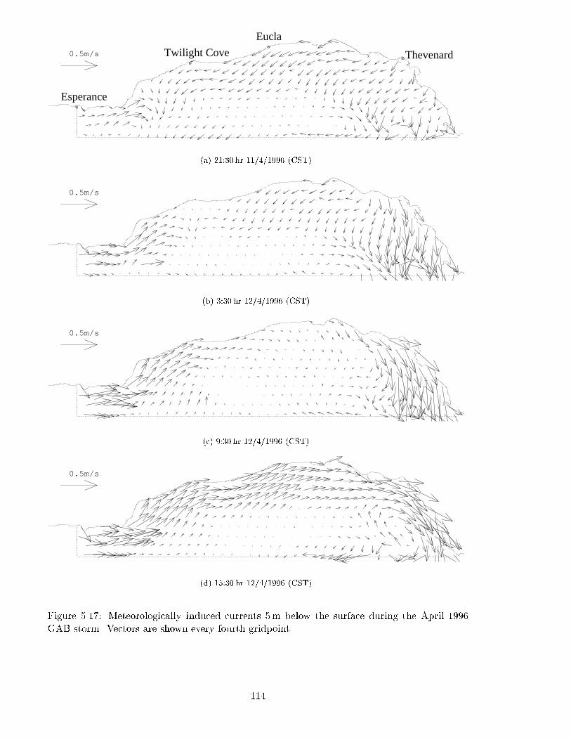
In order to determine the e�ect of the April 1996 GAB storm on the near surface and nearbottom currents, plots of surge associated currents have been produced (Figures 5.17{5.18).These values were obtained by removing tide-only currents from those produced by the stormand tide.

Figure 5.17 shows large storm-induced currents on 12/4/1996, more than twice the speed ofthe tide-induced surface currents shown in Figure 5.10 (note the change of scale). To the south ofThevenard, currents are larger, of the order 0:5m s�1. The pattern of these storm-induced cur-rents varies with the changing wind patterns (see Figure 5.14), going from 0:2m s�1 east-west to0:3m s�1 west-east along the coast, between 21:30 hr 11/4/1996 and 15:30 hr 12/4/1996 (CST).At the latter time, to the east of Eucla, surface tidal currents are directed almost perpendicularto the corresponding storm induced currents.

112

-0.8

-0.6

-0.4

-0.2

0

0.2

0.4

0.6

Res

idua

l Ele

vatio

n (m

)

ModelledRecorded

(a) Surge and Wind

-0.8

-0.6

-0.4

-0.2

0

0.2

0.4

0.6

11/4/96 12/4/96 13/4/96 14/4/96 15/4/96

Res

idua

l Ele

vatio

n (m

)

Time (days, CST)

ModelledRecorded

(b) Surge and Pressure

Figure 5.16: Recorded and computed sea level residuals at Thevenard using either wind orpressure combined with the tide and storm surge on the GAB model open boundary.

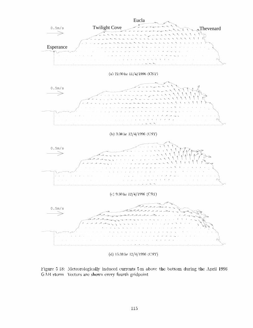
Near the sea oor the meteorologically-induced current speeds (see Figure 5.18) are muchsmaller than at the surface but are still about the same magnitude as the tide-induced surfacecurrents. There is a signi�cant di�erence between surge-associated currents and tidal currents.When surge currents are directed parallel to the coastline, currents at all levels are generally inthe same direction. When surge currents are perpendicular to the coast, surface and bottomcurrents oppose. This contrasts with the tide-only currents, seen in Figures 5.10{5.11, whichare in the same direction at both depths.

One aspect of concern, particularly with the meteorologically induced currents near thesea surface, is the behaviour of the model close to the open boundaries. The open boundaryformulation has been discussed in Section 2.4. It seems that the boundary to the west of theGAB simulates the in ow of water that was caused by the storm quite well. It seems that in thesouth-eastern part of the open boundary, particularly in Figures 5.17(c) and 5.17(d), there maybe some \unreal" ows occurring. These ows are observed close to the shelf edge, in a regionbetween 1000 and 2000m in depth. Initially, it appears that the open boundary condition hasnot been able to cope with the atmospheric forcing applied here. However, the position of the lowpressure system at these times, and the wind direction in this region (Figure 5.13), dominantlyfrom the east along this section of the open boundary, would tend to cause a cross-shelf owas predicted. Such ows are not seen in the near bottom prediction of meteorological currents,further indicating that the wind stress may be responsible for these near surface predictions.

113

Esperance

Twilight Cove

Eucla

Thevenard0.5m/s

(a) 21:30 hr 11/4/1996 (CST)

0.5m/s

(b) 3:30 hr 12/4/1996 (CST)

0.5m/s

(c) 9:30 hr 12/4/1996 (CST)

0.5m/s

(d) 15:30 hr 12/4/1996 (CST)

Figure 5.17: Meteorologically induced currents 5m below the surface during the April 1996GAB storm. Vectors are shown every fourth gridpoint.

114

Esperance

Twilight Cove

Eucla

Thevenard0.5m/s

(a) 21:30 hr 11/4/1996 (CST)

0.5m/s

(b) 3:30 hr 12/4/1996 (CST)

0.5m/s

(c) 9:30 hr 12/4/1996 (CST)

0.5m/s

(d) 15:30 hr 12/4/1996 (CST)

Figure 5.18: Meteorologically induced currents 5m above the bottom during the April 1996GAB storm. Vectors are shown every fourth gridpoint.

115

5.6 Discussion

In the case of the modelling considered in this chapter, the waves observed at Esperance andThevenard are caused by meteorological e�ects, predominantly winds. This agrees with the workof Church and Freeland (1987), who concluded that the GAB shelf waters respond dynamicallyto passing weather systems. However, much of their consideration was with the in uence of theinverse barometric pressure e�ect, whereas it has been found here that the wind e�ect is thedominant in uence on predicted sea levels for this storm.

Krause and Radok (1976) and Provis and Radok (1979) calculated the residuals from sealevel records and concluded that long waves with periods of 4:5 and 9:5 days travelled west toeast across the GAB. This opposes the �ndings here, as do the �ndings of other authors whohave found that coastally trapped waves do propagate around the Great Australian Bight fromwest to east.

It is important to remember that the case considered here is that of a particular stormwhich occurred in April, 1996. In this case, the wind was found to be the dominant sea levelin uence. This may not be true for all scenarios considered within the Bight, but appears tobe the major factor in the storm surge observed in the region in April 1996.

5.7 Summary

A spherical co-ordinate three-dimensional hydrodynamic-numeric GAB model has been pro-duced. This has predicted interesting tidal movements in the region, including ampli�cation ofthe semi-diurnal and ter-diurnal constituents, and near-surface circulation patterns on the shelfedge which are directed to the east and south-east between Eucla and Thevenard, and to thewest and south-west between Esperance and Twilight Cove. At the bottom of the shelf edge,between Eucla and Thevenard, a reasonably strong current to the west occurs both near thesurface and near the sea oor. These predictions agree with tidal current ellipses obtained fromrecorded data (Hahn, 1986).

The GAB model was used to successfully predict the e�ect of the storm of 11{13 April 1996on the sea levels at coastal locations, and the near surface and near bottom currents. It wasfound that the sea level residual on the western boundary propagated only weakly across theGAB, with the main part of the surge recorded at Thevenard caused by the meteorologicale�ects, particularly the wind, acting on the GAB waters.

Storm-induced currents were stronger than the tide-induced currents, and near-surface cur-rents were in the direction of the strong winds. The direction of the storm-induced near-bottomcurrents were the same as those near the surface if currents were directed parallel to the coast,but were opposite to surface currents directed perpendicular to the coast. Further considera-tion of the local e�ects of this storm in Boston Bay, to the east of the GAB, are considered inChapter 8.

116

Chapter 6

Lagrangian{Stochastic Particle

Tracking

6.1 Introduction

The movement and spread of pelagic larvae, �ne sediments and oil slicks due to ocean currentsis of interest and concern to marine scientists, �shermen and conservationists. One way of sim-ulating this movement is through the use of a particle tracking routine which models advectionby a Lagrangian procedure and di�usion by a stochastic process.

This chapter describes the development of a Cartesian co-ordinate pseudo three-dimensionalalgorithm that models these processes in conjunction with the tedmodel described in Chapter 2.Of interest is the e�ect of di�erent grid types upon the behaviour of individual particles atdi�erent regions in a model. In particular, the e�ects near the open (ocean) and closed (coastal)boundaries and in the interior, away from these boundaries, is investigated.

Much of the work in this chapter has been published in Grzechnik and Noye (1998a,b, 1999).

6.2 Oceanographic Modelling of Advection and Di�usion

There are a number of ways of simulating the processes of advection and di�usion in numericalocean models. Two major categories of solution are available, namely Eulerian and Lagrangian,with a hybrid method used in some cases. A summary of these methods is given by Noye (1987).Other processes which depend upon the subject, may also be included within the model. Thesecan include mortality (in the case of larvae), settlement rates (buoyant sediments) or evaporationand emulsi�cation (oil slicks). The work of a number of authors, arranged according to theprocess being simulated, is cited here, with the aim of illustrating the various methods andapplications that can be applied. There will be an emphasis on the Lagrangian method (whichis used here), but other methods will be considered.

6.2.1 Oil spills

The simulation and prediction of oil spill movement has been widely researched over the last10{20 years. Many of the processes that in uence oil dispersal on the sea, including spreading,emulsi�cation and evaporation, are considered by ASCE (1996).

The simulation of oil spills using particle tracking (for advection) and random walk (fordi�usion) methods has been considered by Al-Rabeh and Gunay (1992), Evans and Noye (1995),and Hunter (1987). The advection{di�usion equation, usually using a �nite di�erence scheme,has been considered by Lewis et al. (1996a) and Cuesta et al. (1990). Comparisons betweenthe methods have been made by Lewis et al. (1996b), with both methods found to give similarresults, but the particle tracking method favoured due to its more accurate advection predictionand speed of operation.

117

6.2.2 Larval transport

McShane et al. (1988) and Black and Moran (1991) used a particle tracking method for advectionwith a random walk method simulating di�usion for larvae movement on reefs. Larvae wereconsidered to be neutrally buoyant.

In order to model the advection and di�usion of Penaeus latisulcatus larvae in Spencer Gulf,South Australia, Nixon (1996) applied the Advection{Di�usion{Mortality (ADM) equation.This was solved on a �nite di�erence grid using wind driven currents from a three-dimensionaltidal model. The larvae were considered to be able to control their vertical movement. A concisesummary is considered by Nixon and Noye (1999).

Further consideration of larval transport methods is given in Chapter 7.

Rothlisberg et al. (1996) assumed that prawn larvae were able to control their vertical posi-tion, but moved with the currents in the horizontal directions. A change in vertical behaviourwas considered upon maturity, but the e�ects of di�usion were not considered in this Lagrangianapproach.

6.2.3 Sediment and other transport

The transport of sediments was considered by Noye et al. (1999a) and Black (1987), both usingthe particle tracking technique with random di�usive aspects. The settlement of particles wasconsidered, with importance placed upon modelling the correct physical behaviour of thesesediments.

An application to dispersal of saline water using a combined Euler{Lagrangian methodwas used with success by Cheng et al. (1984). Here advective aspects were calculated using aLagrangian method, and di�usion was calculated in an Eulerian manner.

Some other particle tracking and random walk algorithms have been described by Fogelson(1992), Hunter et al. (1993) and Easton et al. (1996). Application of the particle trackingalgorithm to the dispersal of �ne organic sediment is considered in Chapter 8.

6.2.4 Why the Lagrangian method?

Overall, both methods have their strengths and weaknesses. The particle tracking method ismore e�cient (especially when smaller amounts of particles are used), and generally simulatesadvection more accurately than Eulerian methods. However, the random walk method usedfor simulation of di�usion can introduce some errors, which are not as prevalent in the lattercase. The simulation of larval and sediment movement is considered in this thesis, and theparticle tracking (Lagrangian) method has been chosen for this. This is coupled to a randomwalk method for di�usion, described in this chapter. Alterations to the basic algorithm areconsidered for each type of material dispersal being modelled.

6.3 Advection

In a two-dimensional current �eld, the motion of a particle may be described by

dX

dt= U(X;Y; t); (6.3.1)

dY

dt= V (X;Y; t);

where the symbols used have the following meaning:

t: is the time in seconds (s),

X, Y : are the (time-varying) Cartesian co-ordinates of the particle in metres (m),

118

U , V : are the x, y components of the velocity �eld in m s�1 at (X;Y ). These can be eitheraveraged over depth or the velocity �eld calculated at a particular level or combinationof levels.

In the coastal sea situation, the velocity �eld will usually be determined by means of a tideand storm surge model of the region being considered, in this case the ted model described inChapter 2. In this chapter, the tracking procedure is tested using two di�erent grid structures,as described in Section 6.6. Both structures assume that grid elements are of dimensions 2�x,2�y in the x, y directions respectively (as in Chapter 2). In both cases model boundaries arechosen along grid lines to approximate the shape of the coastal region.

For particles labelled p = 1; 2; 3; : : : ; P , using centred �nite-di�erence approximations forthe time derivative in (6.3.1), applied at the time tn+1=2 = (n + 1=2)�t, n = 0; 1; 2; : : : ; N ,yields

Un+1=2p =

�dX

dt

�n+1=2p

=1

�t(Xn+1

p �Xnp ) +Of(�t)2g; (6.3.2)

V n+1=2p =

�dY

dt

�n+1=2p

=1

�t(Y n+1

p � Y np ) +Of(�t)2g;

in which �t is the positive time step used in the tracking procedure and the superscript indicatesthe time level involved. Time increases from t0 to tN = t0 +N�t in steps of �t.

Rearranging (6.3.2) yields the approximate relations

Xn+1p = Xn

p + Un+1=2p �t; (6.3.3)

Y n+1p = Y n

p + V n+1=2p �t;

in which, to �rst-order,

Un+1=2p = U(Xn

p ; Ynp ; tn+1=2); (6.3.4)

V n+1=2p = V (Xn

p ; Ynp ; tn+1=2):

For modelling of advection, the Courant{Friedrichs{Lewy (CFL) condition (Section 2.7.3)should be satis�ed, namely

cx = U�t=2�x � 1 and cy = V�t=2�y � 1; (6.3.5)

for Courant numbers cx, cy in the x, y directions respectively. This may be re-written in theform

�t � 2minf�x;�ygmaxfU; V g : (6.3.6)

Experience has found that greater accuracy is obtained when smaller time steps are used,so the time step prescribed by (6.3.6) should be considered as an upper limit rather than arecommended value.

6.4 Spatial Interpolation

The velocity at the position (Xnp ; Y

np ) at the time tn+1=2 is determined using bilinear interpola-

tion in space of the velocities computed at the (n+ 1=2) time level, at the velocity gridpointssurrounding the particle (see Evans and Noye, 1995; Grzechnik and Noye, 1998b).

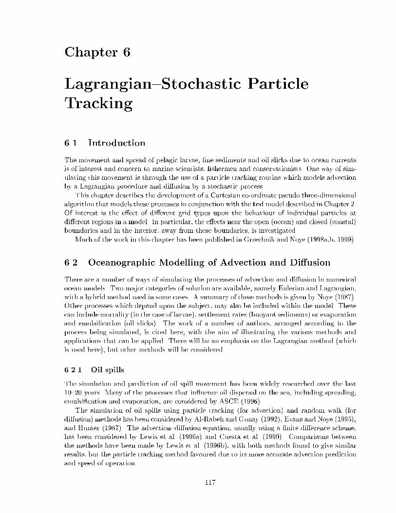
To illustrate the bilinear interpolation scheme, consider U , the x component of velocity. Letparticle p be located at co-ordinates (x0+j 2�x; y0+k 2�y), where 0 � j � 1, 0 � k � 1. At thefour velocity gridpoints surrounding p there are four known values of velocity, UNW ; UNE ; USEand USW (see Figure 6.1). The bilinear interpolation of these values of horizontal velocity yieldsthe approximate x component of velocity of the particle at p, namely

Up = (1� j)(1 � k)USW + j(1 � k)USE + jkUNE + (1� j)kUNW : (6.4.1)

The y component of velocity is approximated similarly.

119

x0 x0 + 2�x

y0

y0 + 2�y

� USW

�UNW

�UNE

�USE

� p6

?

k2�y

-� j2�x

Figure 6.1: The position of the particle p relative to velocity gridpoints in the bilinear interpo-lation.

6.5 Temporal Interpolation

In order to reduce the amount of storage required for velocity input to the tracking routine,a temporal interpolation of velocity values between larger time intervals is carried out. Thisenables velocities to be supplied at time intervals of �T , much greater than �t, and interpolatedto obtain approximate velocity values for use at time steps of �t. For coastal modelling, thevalue of �T usually chosen is one hour, whereas �t may be of the order of minutes, and theinterpolation is usually linear. Testing of the temporal interpolation scheme has been carriedout by Grzechnik and Noye (1998b).

6.6 Grid Types

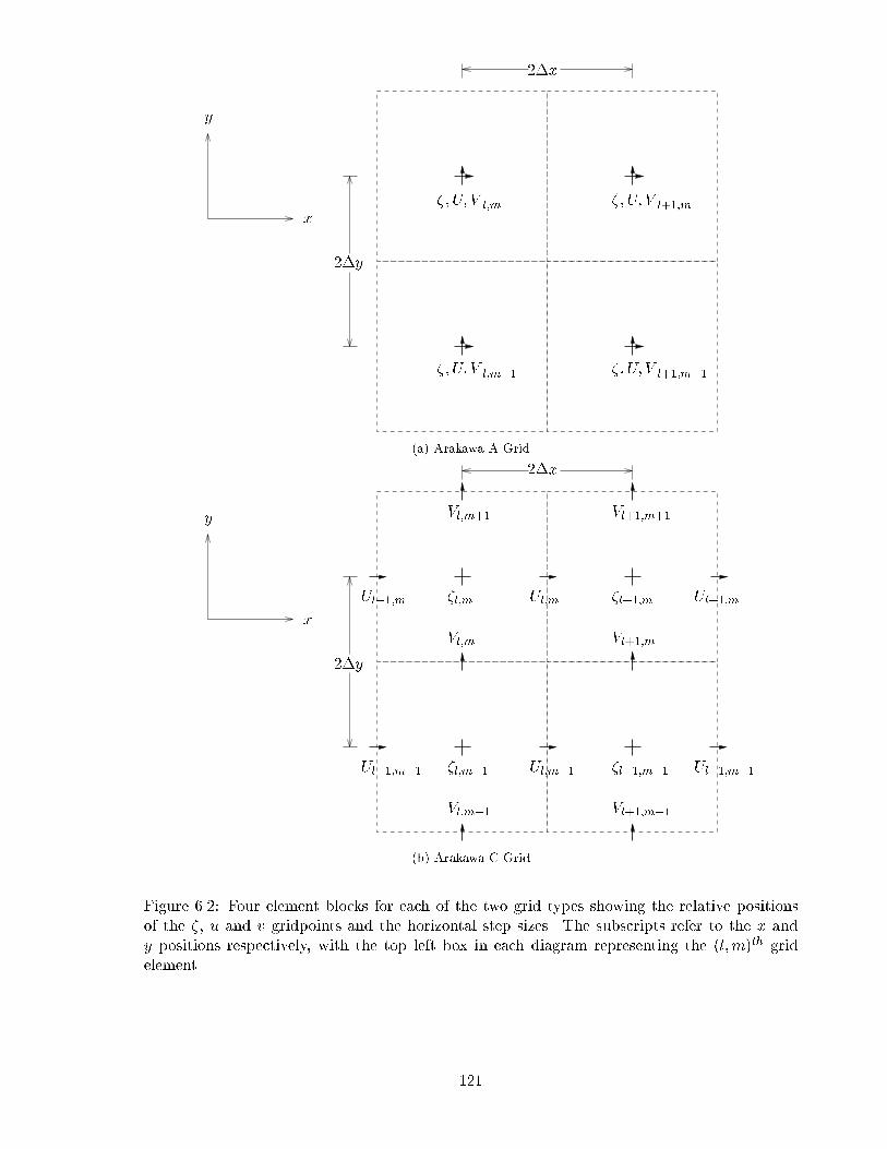
Two possible grid con�gurations are considered for particle tracking. In the �rst (the Arakawa Atype) the elevation and velocity gridpoints coincide, as in Figure 6.2(a), and in the secondthe velocity gridpoints are o�set from the elevation gridpoint (the Arakawa C type) as inFigure 6.2(b) (Arakawa and Lamb, 1977).

The di�erences in the behaviours of the two grid types are of interest due to the nature ofthe tidal models that may be used to produce the velocities. In the ted model used in thiswork (see Chapter 2), the Arakawa C grid con�guration is used during calculation of velocitycomponents, which are then, by averaging, interpolated to the � points in the centre of eachelement, which corresponds then to the Arakawa A type of grid. It is in this way that velocitydata are available for both grid types for use in the particle tracking routine. The e�ect of thisinterpolation on particle movement is investigated here.

In the particle tracker, the Arakawa C grid enables the user to include barriers, that is linesacross which no ow is allowed. Also, a true zero-velocity boundary condition can be appliedat the closed boundaries. The use of the Arakawa A grid simpli�es coding, especially in thecase of the ted model used here, in which the velocity interpolation to the central elevationgridpoint occurs automatically (as described in Section 2.5.8).

The behaviour of particles in the interior of a model region, as well as close to the boundaries,is compared in the following sections.

6.7 Testing Advection in the Model Regions

A number of di�erent tests of the advection of particles have been carried out in the regionmodelled in Figure 6.3, using the grid spacing:

120

y

x

2�y

2�x

�; U; V l;m �; U; V l+1;m

�; U; V l;m�1 �; U; V l+1;m�1

(a) Arakawa A Grid

y

x

2�y

2�x

�l;m �l+1;m

�l;m�1 �l+1;m�1

Ul�1;m Ul;m Ul+1;m

Ul�1;m�1 Ul;m�1 Ul+1;m�1

Vl;m+1 Vl+1;m+1

Vl;m Vl+1;m

Vl;m�1 Vl+1;m�1

(b) Arakawa C Grid

Figure 6.2: Four element blocks for each of the two grid types showing the relative positionsof the �, u and v gridpoints and the horizontal step sizes. The subscripts refer to the x andy positions respectively, with the top left box in each diagram representing the (l;m)th gridelement.

121

0

10

20

30

40

50

60

0 10 20 30 40 50 60

Ver

tical

Dis

tanc

e (k

m)

Horizontal Distance (km)

Exterior

Interior

Coast

Open Boundary

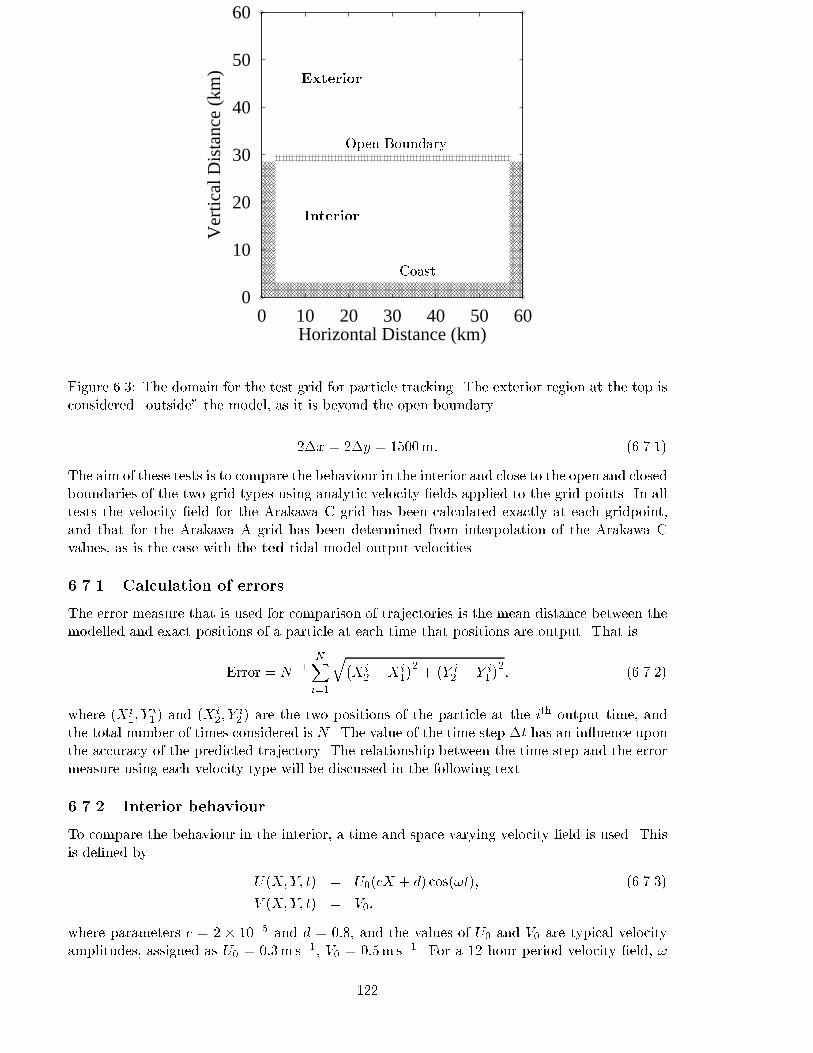
Figure 6.3: The domain for the test grid for particle tracking. The exterior region at the top isconsidered \outside" the model, as it is beyond the open boundary.

2�x = 2�y = 1500m: (6.7.1)

The aim of these tests is to compare the behaviour in the interior and close to the open and closedboundaries of the two grid types using analytic velocity �elds applied to the grid points. In alltests the velocity �eld for the Arakawa C grid has been calculated exactly at each gridpoint,and that for the Arakawa A grid has been determined from interpolation of the Arakawa Cvalues, as is the case with the ted tidal model output velocities.

6.7.1 Calculation of errors

The error measure that is used for comparison of trajectories is the mean distance between themodelled and exact positions of a particle at each time that positions are output. That is

Error = N�1

NXi=1

q�Xi2 �Xi

1

�2+�Y i2 � Y i

1

�2; (6.7.2)

where (Xi1; Y

i1 ) and (Xi

2; Yi2 ) are the two positions of the particle at the ith output time, and

the total number of times considered is N . The value of the time step �t has an in uence uponthe accuracy of the predicted trajectory. The relationship between the time step and the errormeasure using each velocity type will be discussed in the following text.

6.7.2 Interior behaviour

To compare the behaviour in the interior, a time and space varying velocity �eld is used. Thisis de�ned by

U(X;Y; t) = U0(cX + d) cos(!t); (6.7.3)

V (X;Y; t) = V0;

where parameters c = 2 � 10�5 and d = 0:8, and the values of U0 and V0 are typical velocityamplitudes, assigned as U0 = 0:3m s�1, V0 = 0:5m s�1. For a 12 hour period velocity �eld, !

122

is the circular frequency and is assigned the value 2�=(12 � 3600) s�1. The exact solution forparticle motion in this �eld is

X(t) = c�1�(cX0 + d)exp[U0c!

�1 sin(!t)]� d�; (6.7.4)

Y (t) = V0t+ Y0:

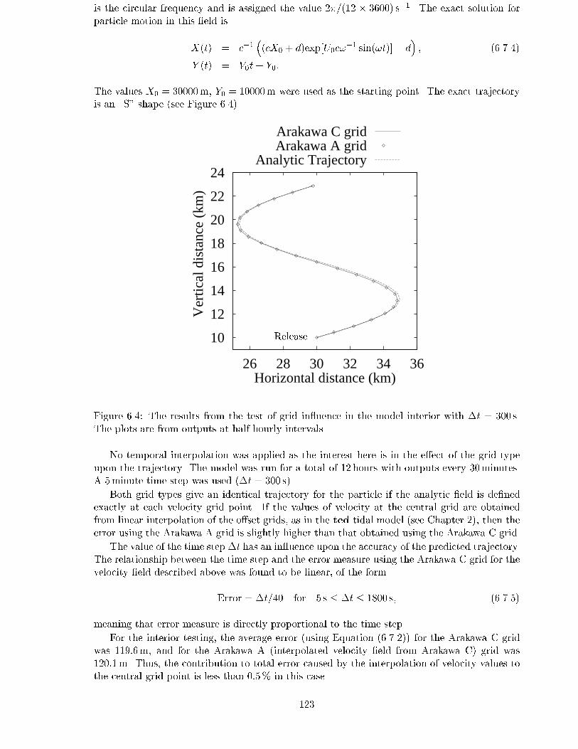
The values X0 = 30000m, Y0 = 10000m were used as the starting point. The exact trajectoryis an \S" shape (see Figure 6.4).

Release10

12

14

16

18

20

22

24

26 28 30 32 34 36

Ver

tical

dis

tanc

e (k

m)

Horizontal distance (km)

Arakawa C gridArakawa A grid

Analytic Trajectory

Figure 6.4: The results from the test of grid in uence in the model interior with �t = 300 s.The plots are from outputs at half hourly intervals.

No temporal interpolation was applied as the interest here is in the e�ect of the grid typeupon the trajectory. The model was run for a total of 12 hours with outputs every 30minutes.A 5minute time step was used (�t = 300 s).

Both grid types give an identical trajectory for the particle if the analytic �eld is de�nedexactly at each velocity grid point. If the values of velocity at the central grid are obtainedfrom linear interpolation of the o�set grids, as in the ted tidal model (see Chapter 2), then theerror using the Arakawa A grid is slightly higher than that obtained using the Arakawa C grid.

The value of the time step �t has an in uence upon the accuracy of the predicted trajectory.The relationship between the time step and the error measure using the Arakawa C grid for thevelocity �eld described above was found to be linear, of the form

Error = �t=40 for 5 s � �t � 1800 s; (6.7.5)

meaning that error measure is directly proportional to the time step.

For the interior testing, the average error (using Equation (6.7.2)) for the Arakawa C gridwas 119:6m, and for the Arakawa A (interpolated velocity �eld from Arakawa C) grid was120:1m. Thus, the contribution to total error caused by the interpolation of velocity values tothe central grid point is less than 0:5% in this case.

123

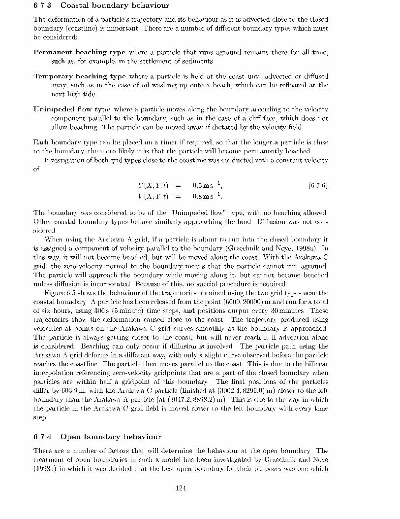
6.7.3 Coastal boundary behaviour

The deformation of a particle's trajectory and its behaviour as it is advected close to the closedboundary (coastline) is important. There are a number of di�erent boundary types which mustbe considered:

Permanent beaching type where a particle that runs aground remains there for all time,such as, for example, in the settlement of sediments.

Temporary beaching type where a particle is held at the coast until advected or di�usedaway, such as in the case of oil washing up onto a beach, which can be re oated at thenext high tide.

Unimpeded ow type where a particle moves along the boundary according to the velocitycomponent parallel to the boundary, such as in the case of a cli� face, which does notallow beaching. The particle can be moved away if dictated by the velocity �eld.

Each boundary type can be placed on a timer if required, so that the longer a particle is closeto the boundary, the more likely it is that the particle will become permanently beached.

Investigation of both grid types close to the coastline was conducted with a constant velocityof

U(X;Y; t) = �0:5m s�1; (6.7.6)

V (X;Y; t) = �0:8m s�1:

The boundary was considered to be of the \Unimpeded ow" type, with no beaching allowed.Other coastal boundary types behave similarly approaching the land. Di�usion was not con-sidered.

When using the Arakawa A grid, if a particle is about to run into the closed boundary itis assigned a component of velocity parallel to the boundary (Grzechnik and Noye, 1998a). Inthis way, it will not become beached, but will be moved along the coast. With the Arakawa Cgrid, the zero-velocity normal to the boundary means that the particle cannot run aground.The particle will approach the boundary while moving along it, but cannot become beachedunless di�usion is incorporated. Because of this, no special procedure is required.

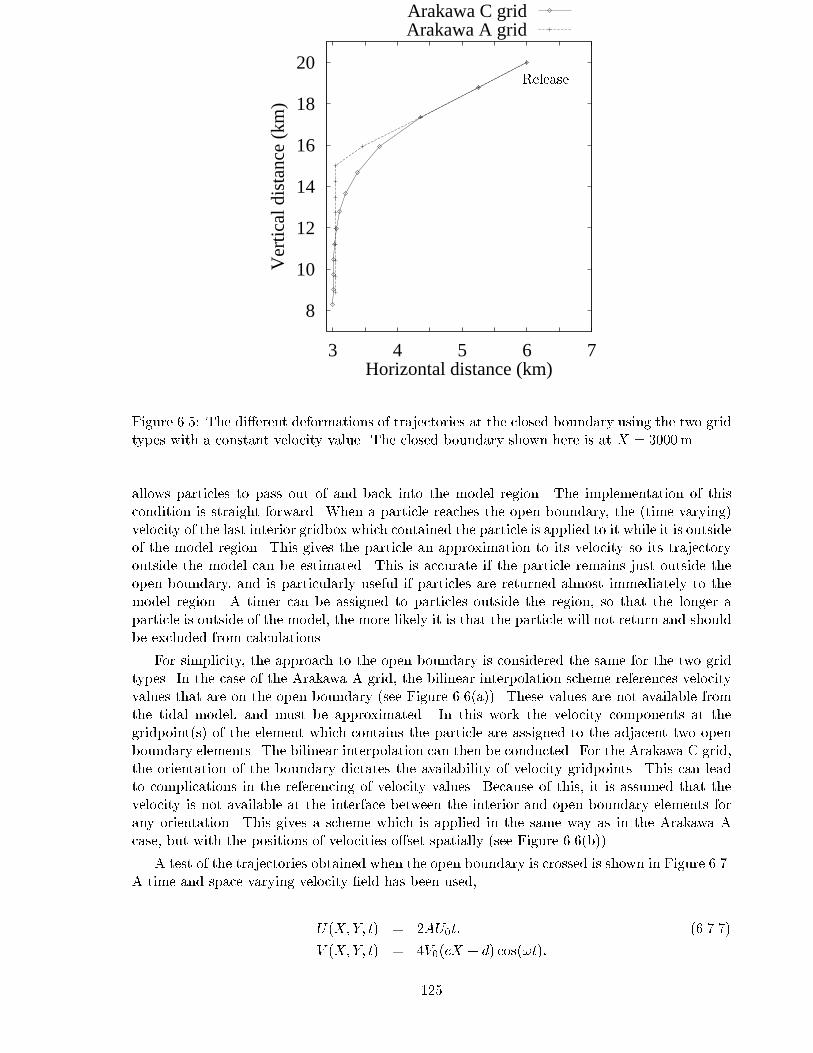
Figure 6.5 shows the behaviour of the trajectories obtained using the two grid types near thecoastal boundary. A particle has been released from the point (6000; 20000)m and run for a totalof six hours, using 300 s (5minute) time steps, and positions output every 30minutes. Thesetrajectories show the deformation caused close to the coast. The trajectory produced usingvelocities at points on the Arakawa C grid curves smoothly as the boundary is approached.The particle is always getting closer to the coast, but will never reach it if advection aloneis considered. Beaching can only occur if di�usion is involved. The particle path using theArakawa A grid deforms in a di�erent way, with only a slight curve observed before the particlereaches the coastline. The particle then moves parallel to the coast. This is due to the bilinearinterpolation referencing zero-velocity gridpoints that are a part of the closed boundary whenparticles are within half a gridpoint of this boundary. The �nal positions of the particlesdi�er by 603:9m, with the Arakawa C particle (�nished at (3002:4; 8296:0)m) closer to the leftboundary than the Arakawa A particle (at (3047:2; 8898:2)m). This is due to the way in whichthe particle in the Arakawa C grid �eld is moved closer to the left boundary with every timestep.

6.7.4 Open boundary behaviour

There are a number of factors that will determine the behaviour at the open boundary. Thetreatment of open boundaries in such a model has been investigated by Grzechnik and Noye(1998a) in which it was decided that the best open boundary for their purposes was one which

124

Release

8

10

12

14

16

18

20

3 4 5 6 7

Ver

tical

dis

tanc

e (k

m)

Horizontal distance (km)

Arakawa C gridArakawa A grid

Figure 6.5: The di�erent deformations of trajectories at the closed boundary using the two gridtypes with a constant velocity value. The closed boundary shown here is at X = 3000m.

allows particles to pass out of and back into the model region. The implementation of thiscondition is straight forward. When a particle reaches the open boundary, the (time varying)velocity of the last interior gridbox which contained the particle is applied to it while it is outsideof the model region. This gives the particle an approximation to its velocity so its trajectoryoutside the model can be estimated. This is accurate if the particle remains just outside theopen boundary, and is particularly useful if particles are returned almost immediately to themodel region. A timer can be assigned to particles outside the region, so that the longer aparticle is outside of the model, the more likely it is that the particle will not return and shouldbe excluded from calculations.

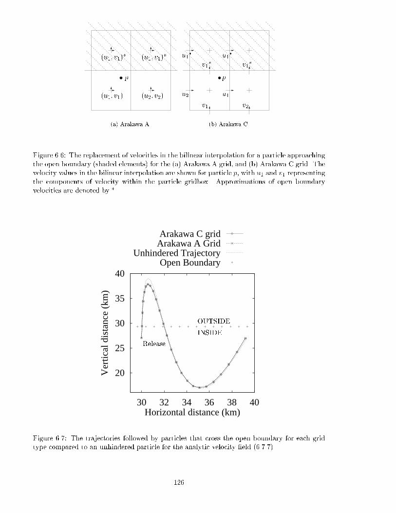
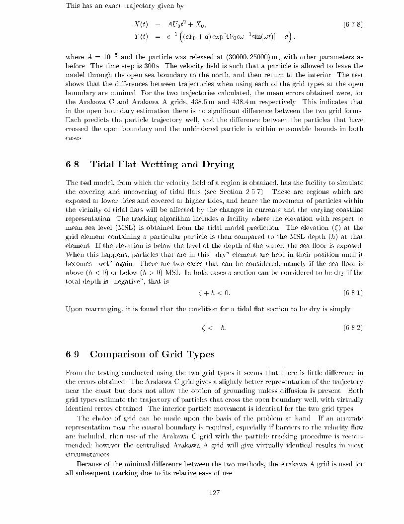
For simplicity, the approach to the open boundary is considered the same for the two gridtypes. In the case of the Arakawa A grid, the bilinear interpolation scheme references velocityvalues that are on the open boundary (see Figure 6.6(a)). These values are not available fromthe tidal model, and must be approximated. In this work the velocity components at thegridpoint(s) of the element which contains the particle are assigned to the adjacent two openboundary elements. The bilinear interpolation can then be conducted. For the Arakawa C grid,the orientation of the boundary dictates the availability of velocity gridpoints. This can leadto complications in the referencing of velocity values. Because of this, it is assumed that thevelocity is not available at the interface between the interior and open boundary elements forany orientation. This gives a scheme which is applied in the same way as in the Arakawa Acase, but with the positions of velocities o�set spatially (see Figure 6.6(b)).

A test of the trajectories obtained when the open boundary is crossed is shown in Figure 6.7.A time and space varying velocity �eld has been used,

U(X;Y; t) = 2AU0t; (6.7.7)

V (X;Y; t) = 4V0(cX + d) cos(!t):

125

(a) Arakawa A (b) Arakawa C

p p

(u1; v1) (u2; v2)

(u1; v1)� (u1; v1)

�

u1u2

u1�u1

�

v1 v2

v1� v1

�

Figure 6.6: The replacement of velocities in the bilinear interpolation for a particle approachingthe open boundary (shaded elements) for the (a) Arakawa A grid, and (b) Arakawa C grid. Thevelocity values in the bilinear interpolation are shown for particle p, with u1 and v1 representingthe components of velocity within the particle gridbox. Approximations of open boundaryvelocities are denoted by �.

Release

OUTSIDE

INSIDE

20

25

30

35

40

30 32 34 36 38 40

Ver

tical

dis

tanc

e (k

m)

Horizontal distance (km)

Arakawa C gridArakawa A Grid

Unhindered TrajectoryOpen Boundary

Figure 6.7: The trajectories followed by particles that cross the open boundary for each gridtype compared to an unhindered particle for the analytic velocity �eld (6.7.7).

126

This has an exact trajectory given by

X(t) = AU0t2 +X0; (6.7.8)

Y (t) = c�1�(cY0 + d) exp[4V0c!

�1sin(!t)]� d�;

where A = 10�5 and the particle was released at (30000; 25000)m, with other parameters asbefore. The time step is 300 s. The velocity �eld is such that a particle is allowed to leave themodel through the open sea boundary to the north, and then return to the interior. The testshows that the di�erences between trajectories when using each of the grid types at the openboundary are minimal. For the two trajectories calculated, the mean errors obtained were, forthe Arakawa C and Arakawa A grids, 438:5m and 438:4m respectively. This indicates thatin the open boundary estimation there is no signi�cant di�erence between the two grid forms.Each predicts the particle trajectory well, and the di�erence between the particles that havecrossed the open boundary and the unhindered particle is within reasonable bounds in bothcases.

6.8 Tidal Flat Wetting and Drying

The ted model, from which the velocity �eld of a region is obtained, has the facility to simulatethe covering and uncovering of tidal ats (see Section 2.5.7). These are regions which areexposed at lower tides and covered at higher tides, and hence the movement of particles withinthe vicinity of tidal ats will be a�ected by the changes in currents and the varying coastlinerepresentation. The tracking algorithm includes a facility where the elevation with respect tomean sea level (MSL) is obtained from the tidal model prediction. The elevation (�) at thegrid element containing a particular particle is then compared to the MSL depth (h) at thatelement. If the elevation is below the level of the depth of the water, the sea oor is exposed.When this happens, particles that are in this \dry" element are held in their position until itbecomes \wet" again. There are two cases that can be considered, namely if the sea oor isabove (h < 0) or below (h > 0) MSL. In both cases a section can be considered to be dry if thetotal depth is \negative", that is

� + h < 0: (6.8.1)

Upon rearranging, it is found that the condition for a tidal at section to be dry is simply

� < �h: (6.8.2)

6.9 Comparison of Grid Types

From the testing conducted using the two grid types it seems that there is little di�erence inthe errors obtained. The Arakawa C grid gives a slightly better representation of the trajectorynear the coast but does not allow the option of grounding unless di�usion is present. Bothgrid types estimate the trajectory of particles that cross the open boundary well, with virtuallyidentical errors obtained. The interior particle movement is identical for the two grid types.

The choice of grid can be made upon the basis of the problem at hand. If an accuraterepresentation near the coastal boundary is required, especially if barriers to the velocity oware included, then use of the Arakawa C grid with the particle tracking procedure is recom-mended; however the centralised Arakawa A grid will give virtually identical results in mostcircumstances.

Because of the minimal di�erence between the two methods, the Arakawa A grid is used forall subsequent tracking due to its relative ease of use.

127

6.10 Di�usion

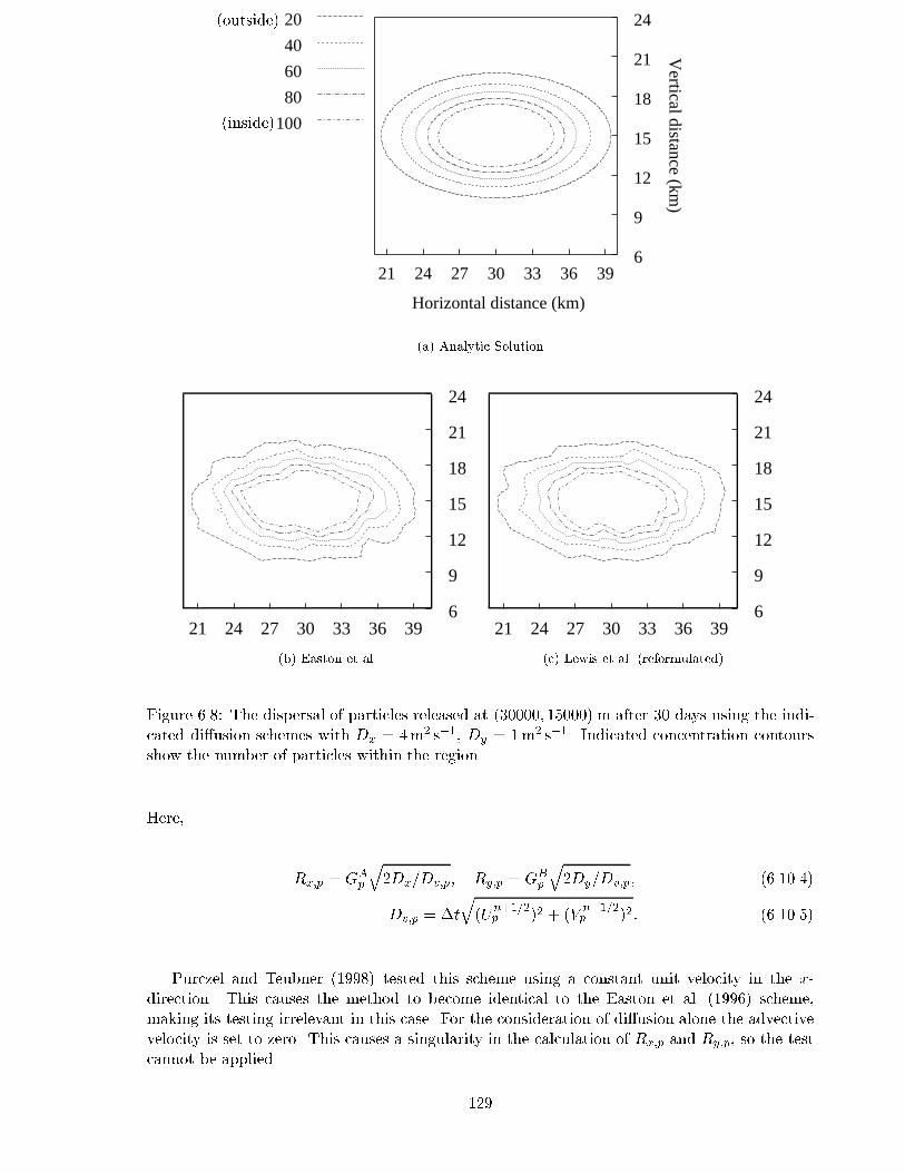
The simulation of di�usion is based upon modi�cations of schemes presented by Easton et al.(1996), Al-Rabeh and Gunay (1992) (later used by Lewis et al. (1996b)) and Prickett et al.(1981). The original versions (with no x- and y- variation) of the �rst of these two have beentested by Grzechnik and Noye (1998b), with dispersals found to be virtually identical. Purczeland Teubner (1998) modi�ed these schemes and tested them for use with di�ering coe�cients ofdi�usion in the x- and y- directions. Unfortunately, the authors misinterpreted several aspectsof the Lewis et al. (1996b) simulation, and obtained erroneous results for the test. Examplesof this are the use of normally distributed rather than uniformly distributed random numbers,as well as incorrectly formulating the dispersal in the case where two directionally di�erentcoe�cients of di�usion are required. The corrected formulation is presented here, and testedagainst the other methods mentioned.

6.10.1 Analytic solution

The analytic solution used is based upon that of Prickett et al. (1981), used by Purczel andTeubner (1998) in testing for application to groundwater ows. The solution has been modi�edto test di�usion only, as advection has been discussed previously, and advection schemes ofall authors mentioned above are implemented identically. The parameters used re ect thoseoccurring in tidal ows, in particular for Gulf St. Vincent, using the test grid described inSection 6.7. The distribution of particles is given by

N(x; y; t) =N0 2�x 2�y

4�tpDxDy

exp

�(x� 30000)2

4Dxt� (y � 15000)2

4Dyt

!; (6.10.1)

where

N0: is the initial number of particles released (5000),

Dx, Dy: are the coe�cients of di�usion (4 and 1m2 s�1 respectively).

The initial release of particles was from the position (30000, 15000) m, and they were releasedfor a total of 30 days. The concentration contours obtained using this analytic solution areshown in Figure 6.8(a).

6.10.2 Easton, Steiner and Zhang

A modi�ed form of the technique of Easton et al. (1996) as presented by Purczel and Teubner(1998) has the form

Xn+1p = Xn

p + Un+1=2p �t+GA

p

p2Dx�t; (6.10.2)

Y n+1p = Y n

p + V n+1=2p �t+GB

p

q2Dy�t:

Here GAp and GB

p are independent random numbers from the standard Gaussian (normal) dis-tribution, with mean 0 and variance 1.

The application of this method to the problem described in Section 6.10.1 is shown inFigure 6.8(b).

6.10.3 Prickett, Naymic and Lonnquist

The scheme of Prickett et al. (1981) as presented by Purczel and Teubner (1998) is as follows.

Xn+1p = Xn

p + (1 +Rx;p)Un+1=2p �t+Ry;pV

n+1=2p �t; (6.10.3)

Y n+1p = Y n

p + (1 +Rx;p)Vn+1=2p �t�Ry;pU

n+1=2p �t:

128

20

40

60

80

100

21 24 27 30 33 36 396

9

12

15

18

21

24

Vertical distance (km

)

Horizontal distance (km)

(a) Analytic Solution

21 24 27 30 33 36 396

9

12

15

18

21

24

(b) Easton et al.

21 24 27 30 33 36 396

9

12

15

18

21

24

(c) Lewis et al. (reformulated)

(outside)

(inside)

Figure 6.8: The dispersal of particles released at (30000; 15000) m after 30 days using the indi-cated di�usion schemes with Dx = 4m2 s�1, Dy = 1m2 s�1. Indicated concentration contoursshow the number of particles within the region.

Here,

Rx;p = GAp

q2Dx=Dv;p; Ry;p = GB

p

q2Dy=Dv;p; (6.10.4)

Dv;p = �t

q(U

n+1=2p )2 + (V

n+1=2p )2: (6.10.5)

Purczel and Teubner (1998) tested this scheme using a constant unit velocity in the x-direction. This causes the method to become identical to the Easton et al. (1996) scheme,making its testing irrelevant in this case. For the consideration of di�usion alone the advectivevelocity is set to zero. This causes a singularity in the calculation of Rx;p and Ry;p, so the testcannot be applied.

129

6.10.4 Lewis, Noye and Evans

The scheme of Lewis et al. (1996b), adapted from Al-Rabeh and Gunay (1992), di�ers fromthose previously considered by utilising uniformly distributed random numbers in the range[0; 1]. These are denoted in the following by JAp , J

Bp . The scheme presented by Purczel and

Teubner (1998) was awed in that it did not take into account the variation of the x- and y-di�usion terms as Dx and Dy were merged into one constant term. The scheme has the form

Xn+1p = Xn

p + Un+1=2p �t+ d1;p cos �p; (6.10.6)

Y n+1p = Y n

p + V n+1=2p �t+ d2;p sin �p;

where �p = 2�JAp , d1;p =p3JBp

p4Dx�t and d2;p =

p3JBp

p4Dy�t.

The results obtained by applying this method are shown in Figure 6.8(c).

6.10.5 Di�usion comparison

It is obvious from Figure 6.8 that the di�usion of particles obtained from the two schemes testedis very good. Both schemes give accurate indications of spreading, with the analytic solutionwell represented. The di�usive spread is independent of the grid type used. The Easton, Steinerand Zhang scheme will be used in the following work.

6.11 Summary

A particle tracking procedure for use in coastal sea modelling has been developed for use withthe ted tide and storm surge model. This procedure has been extensively tested for advection,di�usion and boundary behaviour. It is the aim of this procedure (and the associated com-puter program) to simulate the movement of buoyant particles in the ocean, such as suspendedsediments, oil or pelagic larvae. Applications of the particle tracking routine are considered insubsequent chapters.

130

Chapter 7

Prawn Larvae Dispersal Modelling

in Gulf St. Vincent, South Australia

7.1 Introduction

The dispersal of western king prawn (Penaeus latisulcatus) larvae in Gulf St. Vincent is discussedin this chapter. The underlying tidal and storm surge model, as described in Chapters 3 and 4,is coupled with a wind �eld based upon observations for the times speci�ed to produce currentdata for the region. Measured spawning concentrations are then applied as initial conditions,with current �elds used to drive the particle tracking routine (as described in Chapter 6) andsimulate larval transport until settlement occurs.

Two time periods will be considered, for which spawning and settlement data are available.Comparisons between meteorological and storm induced dispersion of particles and the e�ectsof larval life-stage behaviours will be conducted.

7.2 Prawn Biology

A relatively minor description of the biology of the western king prawn will be considered.Some biological aspects are important in this work, but the emphasis is on modelling and theassociated techniques.

Penaeid prawn species have economical importance throughout the world, comprising mostof the total world catch of prawns, estimated at around 700,000 tonnes per year (Rothschild andBrunenmeister, 1984). In Australia, �sheries exist for a number of penaeid species in NorthernAustralia, New South Wales, South Australia and Western Australia (Kangas, 1999).

Adult females spawn between October and March (King, 1977), and it has been demon-strated by Carrick (1996) that there are two main spawning peaks in November-December andFebruary-March observed through studies in Spencer Gulf, South Australia.

Studies of female prawns from Gulf St. Vincent indicate that a single spawn can yieldbetween 80,000 and 600,000 eggs (Penn, 1980). Spawning may occur more than once in aseason, and adult prawns can live three to four years after recruiting onto the �shing ground.This implies that adult prawns can contribute to egg production more than once (Kangas,1999).

The western king prawn has a life cycle corresponding to that shown in Figure 7.1, wherespawning takes place o�shore and planktonic stages migrate inshore towards the end of larvaldevelopment. The three larval and postlarval stages involved in its development are illustrated.After hatching, prawns develop through the larval stages, namely nauplius, protozoea, zoeaand mysis (Shokita, 1984). When the prawns become postlarvae, they are ready to settle.Laboratory trials for the species have indicated a larval period of 8 days at 29.5�C (Shokita,1984), while the estimate of a 2{4 week period at temperatures between 18�C and 25�C hasbeen made by Penn (1975). In Gulf St. Vincent, observations of postlarval settlement and the

131

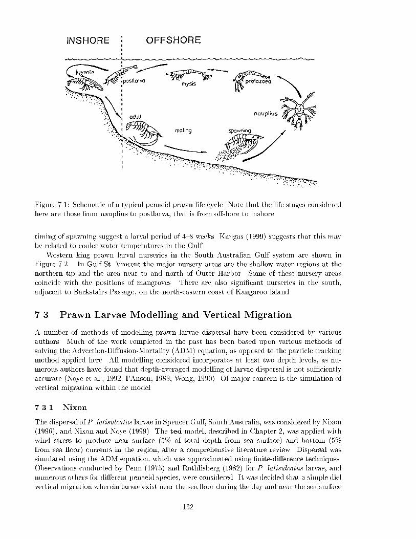
Figure 7.1: Schematic of a typical penaeid prawn life cycle. Note that the life stages consideredhere are those from nauplius to postlarva, that is from o�shore to inshore.

timing of spawning suggest a larval period of 4{8 weeks. Kangas (1999) suggests that this maybe related to cooler water temperatures in the Gulf.

Western king prawn larval nurseries in the South Australian Gulf system are shown inFigure 7.2. In Gulf St. Vincent the major nursery areas are the shallow water regions at thenorthern tip and the area near to and north of Outer Harbor. Some of these nursery areascoincide with the positions of mangroves. There are also signi�cant nurseries in the south,adjacent to Backstairs Passage, on the north-eastern coast of Kangaroo Island.

7.3 Prawn Larvae Modelling and Vertical Migration

A number of methods of modelling prawn larvae dispersal have been considered by variousauthors. Much of the work completed in the past has been based upon various methods ofsolving the Advection-Di�usion-Mortality (ADM) equation, as opposed to the particle trackingmethod applied here. All modelling considered incorporates at least two depth levels, as nu-merous authors have found that depth-averaged modelling of larvae dispersal is not su�cientlyaccurate (Noye et al., 1992; I'Anson, 1989; Wong, 1990). Of major concern is the simulation ofvertical migration within the model.

7.3.1 Nixon

The dispersal of P. latisulcatus larvae in Spencer Gulf, South Australia, was considered by Nixon(1996), and Nixon and Noye (1999). The ted model, described in Chapter 2, was applied withwind stress to produce near surface (5% of total depth from sea surface) and bottom (5%from sea oor) currents in the region, after a comprehensive literature review. Dispersal wassimulated using the ADM equation, which was approximated using �nite-di�erence techniques.Observations conducted by Penn (1975) and Rothlisberg (1982) for P. latisulcatus larvae, andnumerous others for di�erent penaeid species, were considered. It was decided that a simple dielvertical migration wherein larvae exist near the sea oor during the day and near the sea surface

132

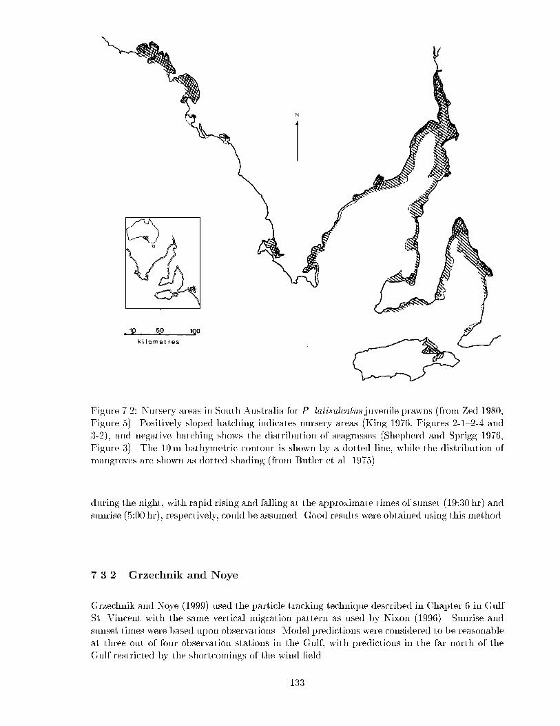
6

N

Figure 7.2: Nursery areas in South Australia for P. latisulcatus juvenile prawns (from Zed 1980,Figure 5). Positively sloped hatching indicates nursery areas (King 1976, Figures 2-1{2-4 and3-2), and negative hatching shows the distribution of seagrasses (Shepherd and Sprigg 1976,Figure 3). The 10m bathymetric contour is shown by a dotted line, while the distribution ofmangroves are shown as dotted shading (from Butler et al. 1975).

during the night, with rapid rising and falling at the approximate times of sunset (19:30 hr) andsunrise (5:00 hr), respectively, could be assumed. Good results were obtained using this method.

7.3.2 Grzechnik and Noye

Grzechnik and Noye (1999) used the particle tracking technique described in Chapter 6 in GulfSt. Vincent with the same vertical migration pattern as used by Nixon (1996). Sunrise andsunset times were based upon observations. Model predictions were considered to be reasonableat three out of four observation stations in the Gulf, with predictions in the far north of theGulf restricted by the shortcomings of the wind �eld.

133

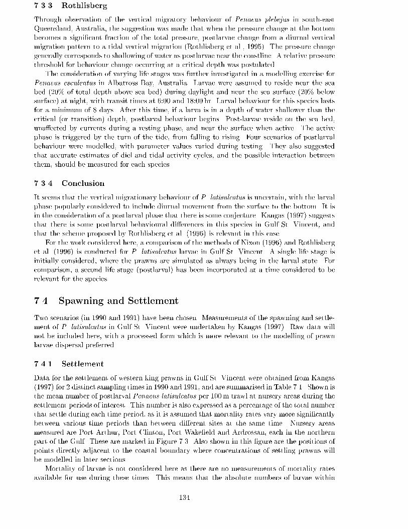
7.3.3 Rothlisberg

Through observation of the vertical migratory behaviour of Penaeus plebejus in south-eastQueensland, Australia, the suggestion was made that when the pressure change at the bottombecomes a signi�cant fraction of the total pressure, postlarvae change from a diurnal verticalmigration pattern to a tidal vertical migration (Rothlisberg et al., 1995). The pressure changegenerally corresponds to shallowing of water as postlarvae near the coastline. A relative pressurethreshold for behaviour change occurring at a critical depth was postulated.

The consideration of varying life stages was further investigated in a modelling exercise forPenaeus esculentus in Albatross Bay, Australia. Larvae were assumed to reside near the seabed (20% of total depth above sea bed) during daylight and near the sea surface (20% belowsurface) at night, with transit times at 6:00 and 18:00 hr. Larval behaviour for this species lastsfor a minimum of 8 days. After this time, if a larva is in a depth of water shallower than thecritical (or transition) depth, postlarval behaviour begins. Post-larvae reside on the sea bed,una�ected by currents during a resting phase, and near the surface when active. The activephase is triggered by the turn of the tide, from falling to rising. Four scenarios of postlarvalbehaviour were modelled, with parameter values varied during testing. They also suggestedthat accurate estimates of diel and tidal activity cycles, and the possible interaction betweenthem, should be measured for each species.

7.3.4 Conclusion

It seems that the vertical migrationary behaviour of P. latisulcatus is uncertain, with the larvalphase popularly considered to include diurnal movement from the surface to the bottom. It isin the consideration of a postlarval phase that there is some conjecture. Kangas (1997) suggeststhat there is some postlarval behavioural di�erences in this species in Gulf St. Vincent, andthat the scheme proposed by Rothlisberg et al. (1996) is relevant in this case.

For the work considered here, a comparison of the methods of Nixon (1996) and Rothlisberget al. (1996) is conducted for P. latisulcatus larvae in Gulf St. Vincent. A single life stage isinitially considered, where the prawns are simulated as always being in the larval state. Forcomparison, a second life stage (postlarval) has been incorporated at a time considered to berelevant for the species.

7.4 Spawning and Settlement

Two scenarios (in 1990 and 1991) have been chosen. Measurements of the spawning and settle-ment of P. latisulcatus in Gulf St. Vincent were undertaken by Kangas (1997). Raw data willnot be included here, with a processed form which is more relevant to the modelling of prawnlarvae dispersal preferred.

7.4.1 Settlement

Data for the settlement of western king prawns in Gulf St. Vincent were obtained from Kangas(1997) for 2 distinct sampling times in 1990 and 1991, and are summarised in Table 7.1. Shown isthe mean number of postlarval Penaeus latisulcatus per 100m trawl at nursery areas during thesettlement periods of interest. This number is also expressed as a percentage of the total numberthat settle during each time period, as it is assumed that mortality rates vary more signi�cantlybetween various time periods than between di�erent sites at the same time. Nursery areasmeasured are Port Arthur, Port Clinton, Port Wake�eld and Ardrossan, each in the northernpart of the Gulf. These are marked in Figure 7.3. Also shown in this �gure are the positions ofpoints directly adjacent to the coastal boundary where concentrations of settling prawns willbe modelled in later sections.

Mortality of larvae is not considered here as there are no measurements of mortality ratesavailable for use during these times. This means that the absolute numbers of larvae within

134

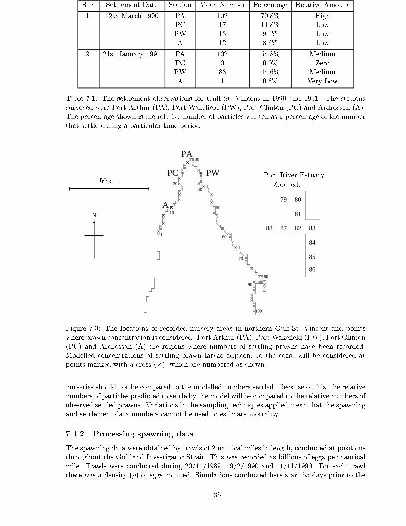
Run Settlement Date Station Mean Number Percentage Relative Amount

1. 12th March 1990 PA 102 70.8% HighPC 17 11.8% LowPW 13 9.1% LowA 12 8.3% Low

2. 21st January 1991 PA 102 54.8% MediumPC 0 0.0% ZeroPW 83 44.6% MediumA 1 0.6% Very Low

Table 7.1: The settlement observations for Gulf St. Vincent in 1990 and 1991. The stationssurveyed were Port Arthur (PA), Port Wake�eld (PW), Port Clinton (PC) and Ardrossan (A).The percentage shown is the relative number of particles written as a percentage of the numberthat settle during a particular time period.

PW

PA

PC

A

1

10

20

30

40

50

60

70

80

90

100

Port River Estuary

Zoomed:

86

85

84

83828788

81

8079

50 km

N

6

Figure 7.3: The locations of recorded nursery areas in northern Gulf St. Vincent and pointswhere prawn concentration is considered. Port Arthur (PA), Port Wake�eld (PW), Port Clinton(PC) and Ardrossan (A) are regions where numbers of settling prawns have been recorded.Modelled concentrations of settling prawn larvae adjacent to the coast will be considered atpoints marked with a cross (�), which are numbered as shown.

nurseries should not be compared to the modelled numbers settled. Because of this, the relativenumbers of particles predicted to settle by the model will be compared to the relative numbers ofobserved settled prawns. Variations in the sampling techniques applied mean that the spawningand settlement data numbers cannot be used to estimate mortality.

7.4.2 Processing spawning data

The spawning data were obtained by trawls of 2 nautical miles in length, conducted at positionsthroughout the Gulf and Investigator Strait. This was recorded as billions of eggs per nauticalmile. Trawls were conducted during 20/11/1989, 19/2/1990 and 11/11/1990. For each trawlthere was a density (�) of eggs counted. Simulations conducted here start 55 days prior to the

135

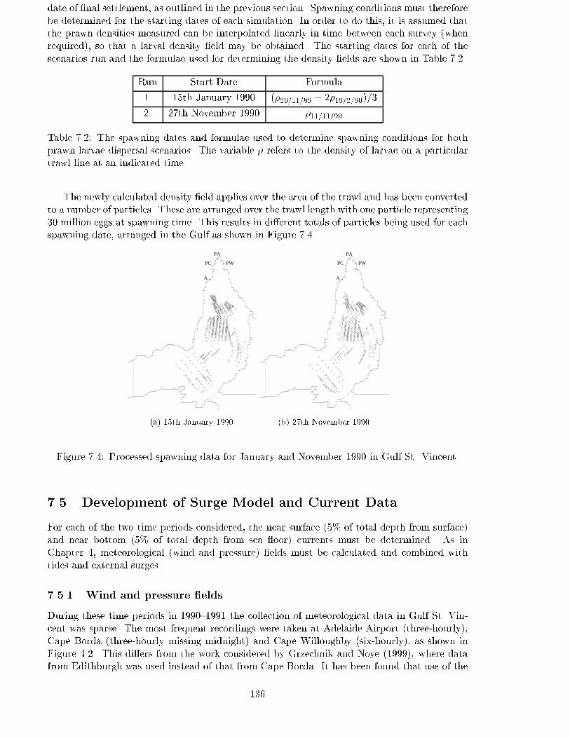
date of �nal settlement, as outlined in the previous section. Spawning conditions must thereforebe determined for the starting dates of each simulation. In order to do this, it is assumed thatthe prawn densities measured can be interpolated linearly in time between each survey (whenrequired), so that a larval density �eld may be obtained. The starting dates for each of thescenarios run and the formulae used for determining the density �elds are shown in Table 7.2.

Run Start Date Formula

1. 15th January 1990 (�20=11=89 + 2�19=2=90)=3

2. 27th November 1990 �11=11=90

Table 7.2: The spawning dates and formulae used to determine spawning conditions for bothprawn larvae dispersal scenarios. The variable � refers to the density of larvae on a particulartrawl line at an indicated time.

The newly calculated density �eld applies over the area of the trawl and has been convertedto a number of particles. These are arranged over the trawl length with one particle representing30 million eggs at spawning time. This results in di�erent totals of particles being used for eachspawning date, arranged in the Gulf as shown in Figure 7.4.

PW

PA

PC

A

(a) 15th January 1990

PW

PA

PC

A

(b) 27th November 1990

Figure 7.4: Processed spawning data for January and November 1990 in Gulf St. Vincent.

7.5 Development of Surge Model and Current Data

For each of the two time periods considered, the near surface (5% of total depth from surface)and near bottom (5% of total depth from sea oor) currents must be determined. As inChapter 4, meteorological (wind and pressure) �elds must be calculated and combined withtides and external surges.

7.5.1 Wind and pressure �elds

During these time periods in 1990{1991 the collection of meteorological data in Gulf St. Vin-cent was sparse. The most frequent recordings were taken at Adelaide Airport (three-hourly),Cape Borda (three-hourly missing midnight) and Cape Willoughby (six-hourly), as shown inFigure 4.2. This di�ers from the work considered by Grzechnik and Noye (1999), where datafrom Edithburgh was used instead of that from Cape Borda. It has been found that use of the

136

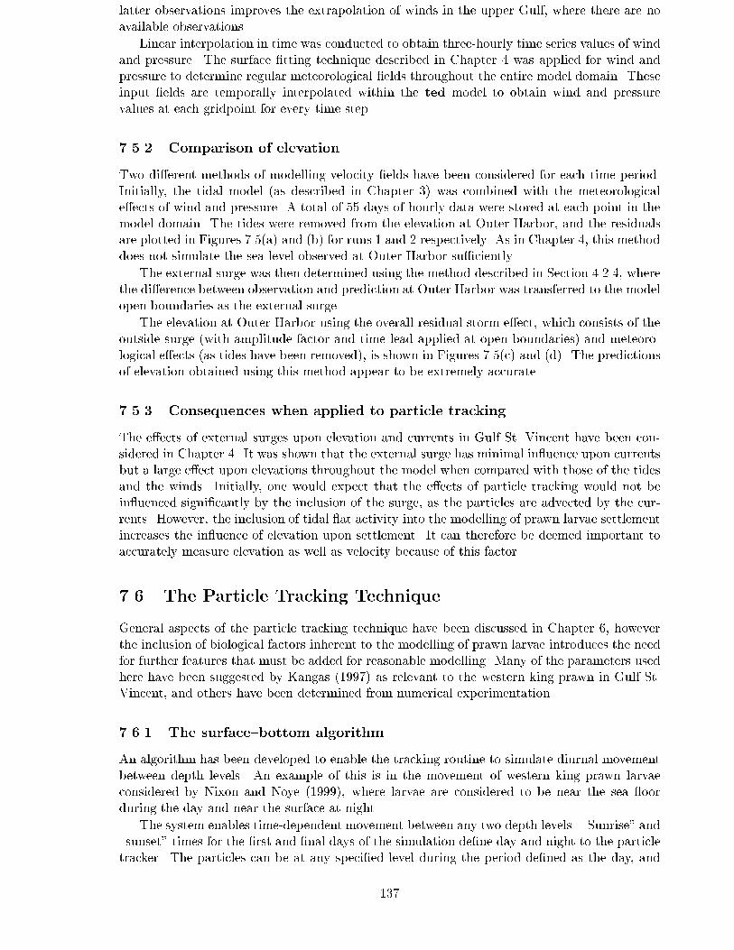
latter observations improves the extrapolation of winds in the upper Gulf, where there are noavailable observations.

Linear interpolation in time was conducted to obtain three-hourly time series values of windand pressure. The surface �tting technique described in Chapter 4 was applied for wind andpressure to determine regular meteorological �elds throughout the entire model domain. Theseinput �elds are temporally interpolated within the ted model to obtain wind and pressurevalues at each gridpoint for every time step.

7.5.2 Comparison of elevation

Two di�erent methods of modelling velocity �elds have been considered for each time period.Initially, the tidal model (as described in Chapter 3) was combined with the meteorologicale�ects of wind and pressure. A total of 55 days of hourly data were stored at each point in themodel domain. The tides were removed from the elevation at Outer Harbor, and the residualsare plotted in Figures 7.5(a) and (b) for runs 1 and 2 respectively. As in Chapter 4, this methoddoes not simulate the sea level observed at Outer Harbor su�ciently.

The external surge was then determined using the method described in Section 4.2.4, wherethe di�erence between observation and prediction at Outer Harbor was transferred to the modelopen boundaries as the external surge.

The elevation at Outer Harbor using the overall residual storm e�ect, which consists of theoutside surge (with amplitude factor and time lead applied at open boundaries) and meteoro-logical e�ects (as tides have been removed), is shown in Figures 7.5(c) and (d). The predictionsof elevation obtained using this method appear to be extremely accurate.

7.5.3 Consequences when applied to particle tracking

The e�ects of external surges upon elevation and currents in Gulf St. Vincent have been con-sidered in Chapter 4. It was shown that the external surge has minimal in uence upon currentsbut a large e�ect upon elevations throughout the model when compared with those of the tidesand the winds. Initially, one would expect that the e�ects of particle tracking would not bein uenced signi�cantly by the inclusion of the surge, as the particles are advected by the cur-rents. However, the inclusion of tidal at activity into the modelling of prawn larvae settlementincreases the in uence of elevation upon settlement. It can therefore be deemed important toaccurately measure elevation as well as velocity because of this factor.

7.6 The Particle Tracking Technique

General aspects of the particle tracking technique have been discussed in Chapter 6, howeverthe inclusion of biological factors inherent to the modelling of prawn larvae introduces the needfor further features that must be added for reasonable modelling. Many of the parameters usedhere have been suggested by Kangas (1997) as relevant to the western king prawn in Gulf St.Vincent, and others have been determined from numerical experimentation.

7.6.1 The surface{bottom algorithm

An algorithm has been developed to enable the tracking routine to simulate diurnal movementbetween depth levels. An example of this is in the movement of western king prawn larvaeconsidered by Nixon and Noye (1999), where larvae are considered to be near the sea oorduring the day and near the surface at night.

The system enables time-dependent movement between any two depth levels. \Sunrise" and\sunset" times for the �rst and �nal days of the simulation de�ne day and night to the particletracker. The particles can be at any speci�ed level during the period de�ned as the day, and

137

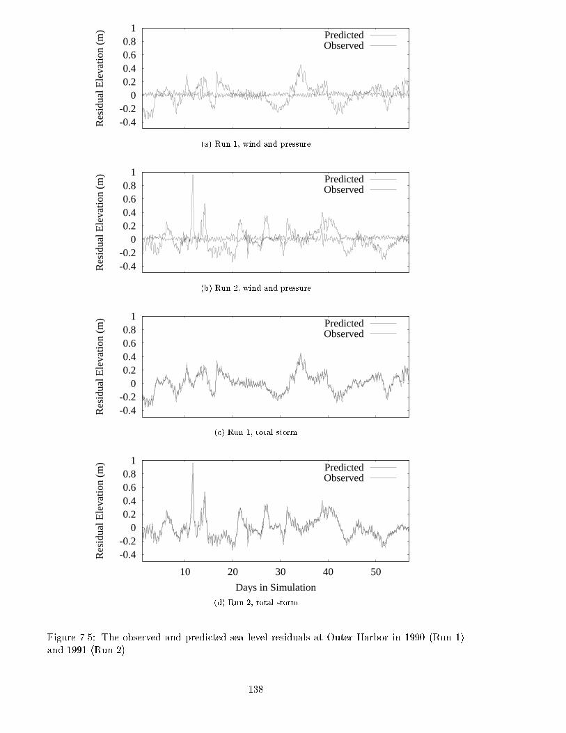
-0.4-0.2

00.20.40.60.8

1

Res

idua

l Ele

vatio

n (m

) PredictedObserved

(a) Run 1, wind and pressure

-0.4-0.2

00.20.40.60.8

1

Res

idua

l Ele

vatio

n (m

) PredictedObserved

(b) Run 2, wind and pressure

-0.4-0.2

00.20.40.60.8

1

Res

idua

l Ele

vatio

n (m

) PredictedObserved

(c) Run 1, total storm

-0.4-0.2

00.20.40.60.8

1

10 20 30 40 50

Res

idua

l Ele

vatio

n (m

)

Days in Simulation

PredictedObserved

(d) Run 2, total storm

Figure 7.5: The observed and predicted sea level residuals at Outer Harbor in 1990 (Run 1)and 1991 (Run 2).

138

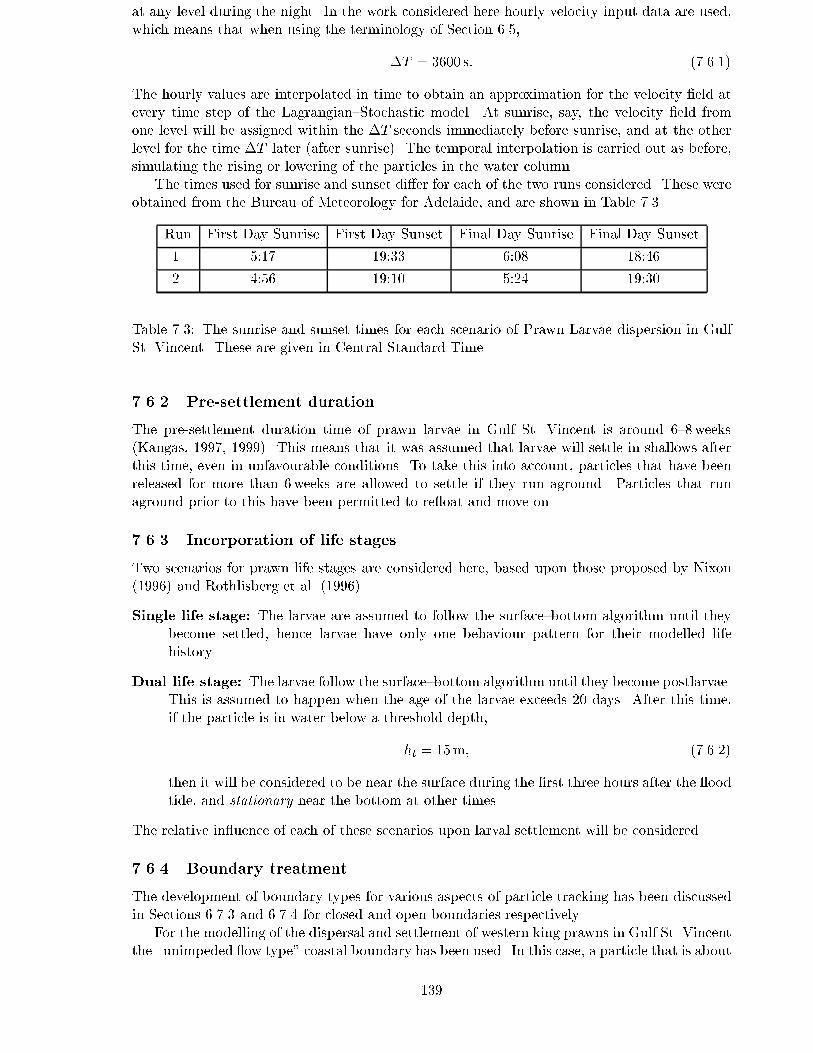
at any level during the night. In the work considered here hourly velocity input data are used,which means that when using the terminology of Section 6.5,

�T = 3600 s: (7.6.1)

The hourly values are interpolated in time to obtain an approximation for the velocity �eld atevery time step of the Lagrangian{Stochastic model. At sunrise, say, the velocity �eld fromone level will be assigned within the �T seconds immediately before sunrise, and at the otherlevel for the time �T later (after sunrise). The temporal interpolation is carried out as before,simulating the rising or lowering of the particles in the water column.

The times used for sunrise and sunset di�er for each of the two runs considered. These wereobtained from the Bureau of Meteorology for Adelaide, and are shown in Table 7.3.

Run First Day Sunrise First Day Sunset Final Day Sunrise Final Day Sunset

1. 5:17 19:33 6:08 18:46

2. 4:56 19:10 5:24 19:30

Table 7.3: The sunrise and sunset times for each scenario of Prawn Larvae dispersion in GulfSt. Vincent. These are given in Central Standard Time.

7.6.2 Pre-settlement duration

The pre-settlement duration time of prawn larvae in Gulf St. Vincent is around 6{8weeks(Kangas, 1997, 1999). This means that it was assumed that larvae will settle in shallows afterthis time, even in unfavourable conditions. To take this into account, particles that have beenreleased for more than 6weeks are allowed to settle if they run aground. Particles that runaground prior to this have been permitted to re oat and move on.

7.6.3 Incorporation of life stages

Two scenarios for prawn life stages are considered here, based upon those proposed by Nixon(1996) and Rothlisberg et al. (1996).

Single life stage: The larvae are assumed to follow the surface{bottom algorithm until theybecome settled, hence larvae have only one behaviour pattern for their modelled lifehistory.

Dual life stage: The larvae follow the surface{bottom algorithm until they become postlarvae.This is assumed to happen when the age of the larvae exceeds 20 days. After this time,if the particle is in water below a threshold depth,

ht = 15m; (7.6.2)

then it will be considered to be near the surface during the �rst three hours after the oodtide, and stationary near the bottom at other times.

The relative in uence of each of these scenarios upon larval settlement will be considered.

7.6.4 Boundary treatment

The development of boundary types for various aspects of particle tracking has been discussedin Sections 6.7.3 and 6.7.4 for closed and open boundaries respectively.

For the modelling of the dispersal and settlement of western king prawns in Gulf St. Vincentthe \unimpeded ow type" coastal boundary has been used. In this case, a particle that is about

139

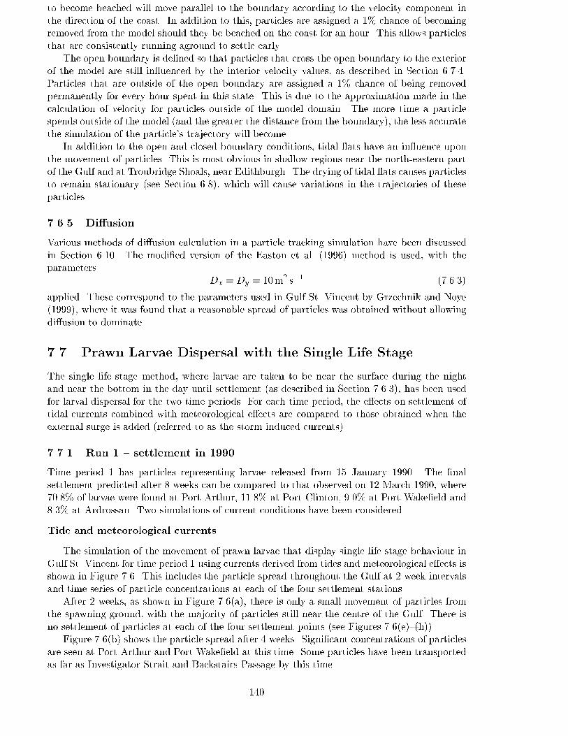
to become beached will move parallel to the boundary according to the velocity component inthe direction of the coast. In addition to this, particles are assigned a 1% chance of becomingremoved from the model should they be beached on the coast for an hour. This allows particlesthat are consistently running aground to settle early.

The open boundary is de�ned so that particles that cross the open boundary to the exteriorof the model are still in uenced by the interior velocity values, as described in Section 6.7.4.Particles that are outside of the open boundary are assigned a 1% chance of being removedpermanently for every hour spent in this state. This is due to the approximation made in thecalculation of velocity for particles outside of the model domain. The more time a particlespends outside of the model (and the greater the distance from the boundary), the less accuratethe simulation of the particle's trajectory will become.

In addition to the open and closed boundary conditions, tidal ats have an in uence uponthe movement of particles. This is most obvious in shallow regions near the north-eastern partof the Gulf and at Troubridge Shoals, near Edithburgh. The drying of tidal ats causes particlesto remain stationary (see Section 6.8), which will cause variations in the trajectories of theseparticles.

7.6.5 Di�usion

Various methods of di�usion calculation in a particle tracking simulation have been discussedin Section 6.10. The modi�ed version of the Easton et al. (1996) method is used, with theparameters

Dx = Dy = 10m2 s�1 (7.6.3)

applied. These correspond to the parameters used in Gulf St. Vincent by Grzechnik and Noye(1999), where it was found that a reasonable spread of particles was obtained without allowingdi�usion to dominate.

7.7 Prawn Larvae Dispersal with the Single Life Stage

The single life stage method, where larvae are taken to be near the surface during the nightand near the bottom in the day until settlement (as described in Section 7.6.3), has been usedfor larval dispersal for the two time periods. For each time period, the e�ects on settlement oftidal currents combined with meteorological e�ects are compared to those obtained when theexternal surge is added (referred to as the storm induced currents).

7.7.1 Run 1 { settlement in 1990

Time period 1 has particles representing larvae released from 15 January 1990. The �nalsettlement predicted after 8 weeks can be compared to that observed on 12 March 1990, where70.8% of larvae were found at Port Arthur, 11.8% at Port Clinton, 9.0% at Port Wake�eld and8.3% at Ardrossan. Two simulations of current conditions have been considered.

Tide and meteorological currents

The simulation of the movement of prawn larvae that display single life stage behaviour inGulf St. Vincent for time period 1 using currents derived from tides and meteorological e�ects isshown in Figure 7.6. This includes the particle spread throughout the Gulf at 2 week intervalsand time series of particle concentrations at each of the four settlement stations.

After 2 weeks, as shown in Figure 7.6(a), there is only a small movement of particles fromthe spawning ground, with the majority of particles still near the centre of the Gulf. There isno settlement of particles at each of the four settlement points (see Figures 7.6(e){(h)).

Figure 7.6(b) shows the particle spread after 4 weeks. Signi�cant concentrations of particlesare seen at Port Arthur and Port Wake�eld at this time. Some particles have been transportedas far as Investigator Strait and Backstairs Passage by this time.

140

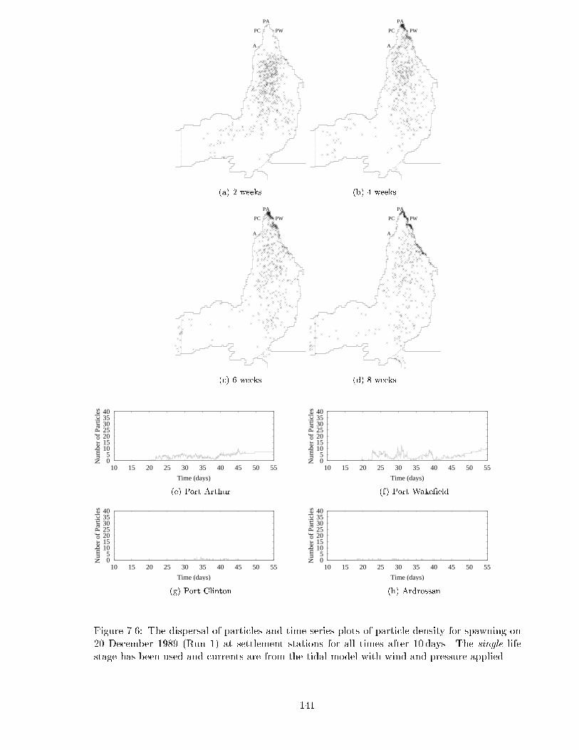
PW

PA

PC

A

(a) 2 weeks

PW

PA

PC

A

(b) 4 weeks

PW

PA

PC

A

(c) 6 weeks

PW

PA

PC

A

(d) 8 weeks

05

10152025303540

10 15 20 25 30 35 40 45 50 55

Num

ber

of P

artic

les

Time (days)

(e) Port Arthur

05

10152025303540

10 15 20 25 30 35 40 45 50 55

Num

ber

of P

artic

les

Time (days)

(f) Port Wake�eld

05

10152025303540

10 15 20 25 30 35 40 45 50 55

Num

ber

of P

artic

les

Time (days)

(g) Port Clinton

05

10152025303540

10 15 20 25 30 35 40 45 50 55

Num

ber

of P

artic

les

Time (days)

(h) Ardrossan

Figure 7.6: The dispersal of particles and time series plots of particle density for spawning on20 December 1989 (Run 1) at settlement stations for all times after 10 days. The single lifestage has been used and currents are from the tidal model with wind and pressure applied.

141

Two weeks later (6 weeks after spawning) more particles appear near Ports Arthur andWake�eld (Figure 7.6(c)). A few particles are also present at Ardrossan and Port Clinton, butnot in signi�cant numbers. Some particles have crossed the Investigator Strait and BackstairsPassage open boundaries, a proportion of which are still active at this time. The pre-settlementduration time has been set to 6 weeks, so particles that reach the coast after this time will berecruited to the nursery.

The �nal snapshot of particle concentration after 8 weeks is presented in Figure 7.6(d).More particles have settled over the �nal two week period, particularly on the north-easterncoast of the Gulf. The major concentrations of particles occur at the major nursery areas inthis part of the Gulf.

Figures 7.6(e){(h) show the time series of particle density at each of the four points wheresettlement data are available. The most signi�cant settlement occurred at Port Arthur andPort Wake�eld, with �nal concentrations of 7 and 9 particles respectively. No particles settledat Port Clinton or Ardrossan.

Storm induced currents

The simulation of prawn larvae which exhibit single life stage behaviour in Gulf St. Vincentfor time period 1 using currents derived from tides, external surges and meteorological e�ectsis shown in Figure 7.7. The dispersal of particles is very similar to that obtained when externalsurges are not included, which is expected due to the small e�ect that this factor was found tohave on currents within the region in Chapter 4.

Particle dispersal after 2, 4, 6 and 8 weeks is shown in Figures 7.7(a){(d). As for the non-surge case, the concentrations of particles at Ports Arthur and Wake�eld are signi�cant. The�nal settlement of particles shows the north-eastern coast from Port Arthur to Outer Harborcovered with the majority of settling particles.

The time series plots of particle density, shown in Figures 7.7(e){(h), illustrate that there isslightly less settlement at Port Arthur and Port Wake�eld than in the case where storm surgee�ects are not included, with 4 and 7 particles settling respectively. As previously, no particlessettled at Port Clinton or Ardrossan.

7.7.2 Run 2 { settlement in 1991

Time period 2 has particles representing larvae released from 27 November 1990. The �nalsettlement predicted after 8 weeks can be compared to that observed on 21 January 1991, where54.8% of larvae were found at Port Arthur, 0.0% at Port Clinton, 44.6% at Port Wake�eld and0.6% at Ardrossan. Two simulations of current conditions have been considered.

Tide and meteorological currents

The simulation of prawns that exhibit single life stage behaviour during time period 2 withcurrents derived from tides and meteorological e�ects is shown in Figure 7.8.

The dispersal of particles in the �rst 4 weeks shows that there are very few particles thatreach the four settlement observation points, with only two particles near Port Wake�eld atthis time (see Figures 7.8(a){(b)). The major grouping of particles appears to be in the tidal at region to the south of Port Wake�eld.

After 6 weeks, in Figure 7.8(c), there are a few particles near Port Wake�eld but none at theother stations. The majority of particles are in the region south of Port Wake�eld and northof Outer Harbor. Additionally, very few particles cross the open boundary compared to thosein time period 1.

Final settlement concentrations after 8 weeks are shown in Figure 7.8(d). Port Wake�eld isagain the only settlement point with particle coverage. Beached particles are predominantly inthe tidal at region from Outer Harbor to Port Wake�eld.

The time series plots of particle settlement at each of the four settlement points are shownin Figures 7.8(e){(h). There is no settlement of particles at Port Clinton and Ardrossan at any

142

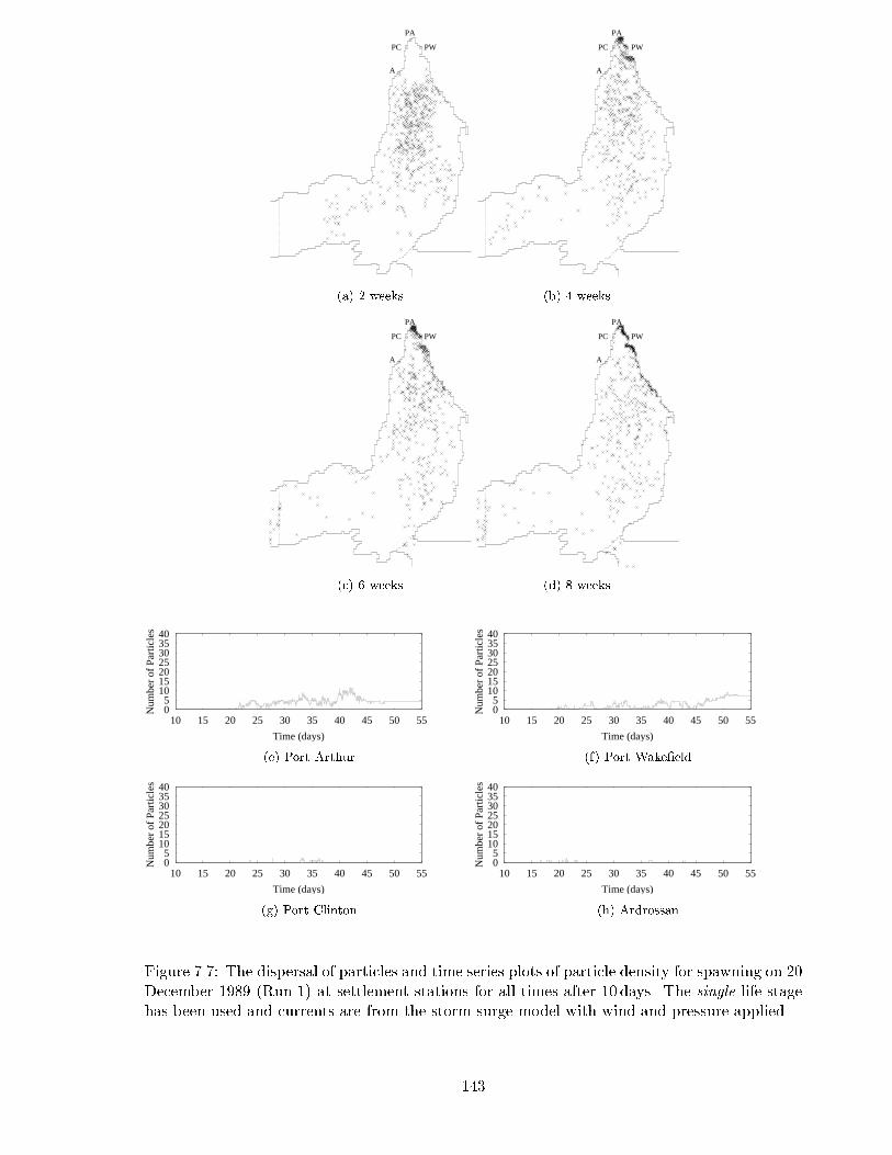
PW

PA

PC

A

(a) 2 weeks

PW

PA

PC

A

(b) 4 weeks

PW

PA

PC

A

(c) 6 weeks

PW

PA

PC

A

(d) 8 weeks

05

10152025303540

10 15 20 25 30 35 40 45 50 55

Num

ber

of P

artic

les

Time (days)

(e) Port Arthur

05

10152025303540

10 15 20 25 30 35 40 45 50 55

Num

ber

of P

artic

les

Time (days)

(f) Port Wake�eld

05

10152025303540

10 15 20 25 30 35 40 45 50 55

Num

ber

of P

artic

les

Time (days)

(g) Port Clinton

05

10152025303540

10 15 20 25 30 35 40 45 50 55

Num

ber

of P

artic

les

Time (days)

(h) Ardrossan

Figure 7.7: The dispersal of particles and time series plots of particle density for spawning on 20December 1989 (Run 1) at settlement stations for all times after 10 days. The single life stagehas been used and currents are from the storm surge model with wind and pressure applied.

143

PW

PA

PC

A

(a) 2 weeks

PW

PA

PC

A

(b) 4 weeks

PW

PA

PC

A

(c) 6 weeks

PW

PA

PC

A

(d) 8 weeks

05

10152025303540

10 15 20 25 30 35 40 45 50 55

Num

ber

of P

artic

les

Time (days)

(e) Port Arthur

05

10152025303540

10 15 20 25 30 35 40 45 50 55

Num

ber

of P

artic

les

Time (days)

(f) Port Wake�eld

05

10152025303540

10 15 20 25 30 35 40 45 50 55

Num

ber

of P

artic

les

Time (days)

(g) Port Clinton

05

10152025303540

10 15 20 25 30 35 40 45 50 55

Num

ber

of P

artic

les

Time (days)

(h) Ardrossan

Figure 7.8: The dispersal of particles and time series plots of particle density for spawning on15 January 1990 (Run 2) at settlement stations for all times after 10 days. The single life stagehas been used and currents are from the tidal model with wind and pressure applied.

144

time of the simulation, and Port Arthur has only a single particle between 40 and 50 days, butthere are no particles that settle after 8 weeks. At Port Wake�eld there is a �nal concentrationof 1 particle, and a maximum value of 5 particles is reached between 40 and 45 days.

Storm induced currents

The simulation of the transport of prawn larvae that exhibit single life stage behaviour duringtime period 2 with currents derived from tides, external surges and meteorological e�ects (thestorm) is shown in Figure 7.9.

As for time period 1, the dispersal and settlement of particles for this case is similar to whentides, wind and pressure e�ects only are used. Over the 8 week simulation it is obvious that theonly station which is inundated with particles is Port Wake�eld, with particles generally absentfrom the other three. The �nal settlement, shown in Figure 7.9(d), illustrates that particlesmainly settle on the eastern coast between Outer Harbor and the head of the Gulf (north ofPort Wake�eld).

Figures 7.9(e){(h) show time series plots of particle concentrations at each of the fourstations. As in the case when external surges were not included, there is no settlement ofparticles at Port Arthur, Port Clinton or Ardrossan. At Port Wake�eld there is increasedsettlement, with a �nal concentration of 5 particles predicted.

7.8 Prawn Larvae Dispersion with Dual Life Stages

The dual life stage behaviour model, where prawns are taken to be near the surface during thenight and the bottom in the day whilst in the larval stage, and behave di�erently when theybecome postlarvae (as described in Section 7.6.3), has been used for larval dispersal for the twotime periods. For each time period, the e�ects upon settlement of tidal currents combined withmeteorological e�ects are compared to those obtained when the external surge is added (thestorm induced currents).

7.8.1 Run 1 { settlement in 1990

Tide and meteorological currents

The simulation of prawn dispersal with the application of dual life stage behaviour and cur-rents derived from tides and meteorological e�ects during time period 1 is shown in Figure 7.10.

The particles behave identically to those for the single life stage for the �rst 20 days, andthere are some slight di�erences after 4 weeks (see Figure 7.10(b)). At this time there areparticles at the three northern settlement stations.

The dispersal of particles after 6 weeks in Figure 7.10(c) is very di�erent to that of the singlelife stage, with many of the particles transported close to the coastal boundary, particularly inthe northern part of the Gulf. There are particles inside the Port River Estuary on the easterncoast north of Outer Harbor, and very few particles have left the model via the open boundary.

The �nal settlement after 8 weeks shows large numbers of particles at Port Arthur and PortWake�eld, with smaller numbers at Port Clinton and Ardrossan (see Figure 7.10(d)). Thereare some particles that have settled near the Outer Harbor region.

The time series of particle concentration at each of the four stations show remarkable di�er-ences to that obtained when single life stage behaviour is applied. In each case, the concentrationof particles is signi�cantly higher than that obtained previously. After 55 days there were 36particles at Port Arthur, 13 at Port Wake�eld, 2 at Port Clinton and 2 at Ardrossan.

Storm induced currents

The storm driven dispersal of particles which exhibit dual life stage behaviour for timeperiod 1 is shown in Figure 7.11.

145

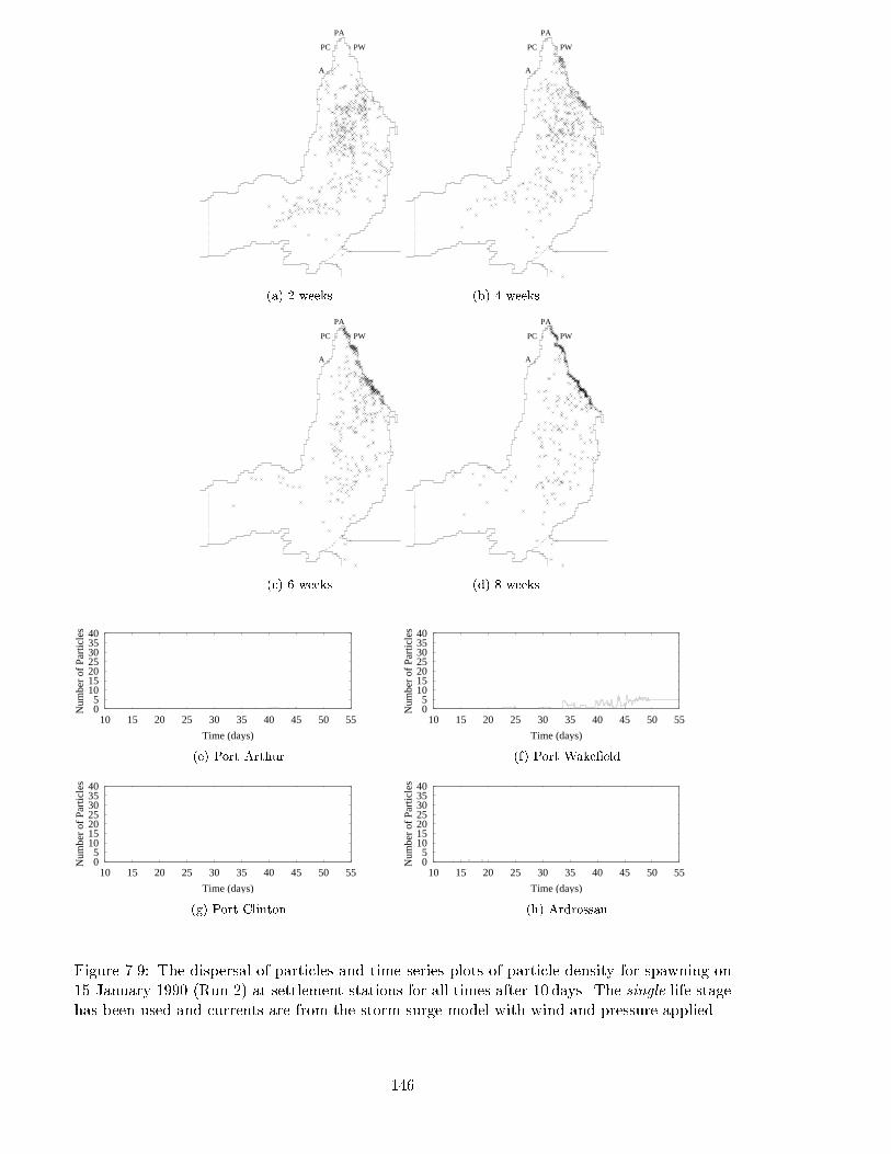
PW

PA

PC

A

(a) 2 weeks

PW

PA

PC

A

(b) 4 weeks

PW

PA

PC

A

(c) 6 weeks

PW

PA

PC

A

(d) 8 weeks

05

10152025303540

10 15 20 25 30 35 40 45 50 55

Num

ber

of P

artic

les

Time (days)

(e) Port Arthur

05

10152025303540

10 15 20 25 30 35 40 45 50 55

Num

ber

of P

artic

les

Time (days)

(f) Port Wake�eld

05

10152025303540

10 15 20 25 30 35 40 45 50 55

Num

ber

of P

artic

les

Time (days)

(g) Port Clinton

05

10152025303540

10 15 20 25 30 35 40 45 50 55

Num

ber

of P

artic

les

Time (days)

(h) Ardrossan

Figure 7.9: The dispersal of particles and time series plots of particle density for spawning on15 January 1990 (Run 2) at settlement stations for all times after 10 days. The single life stagehas been used and currents are from the storm surge model with wind and pressure applied.

146

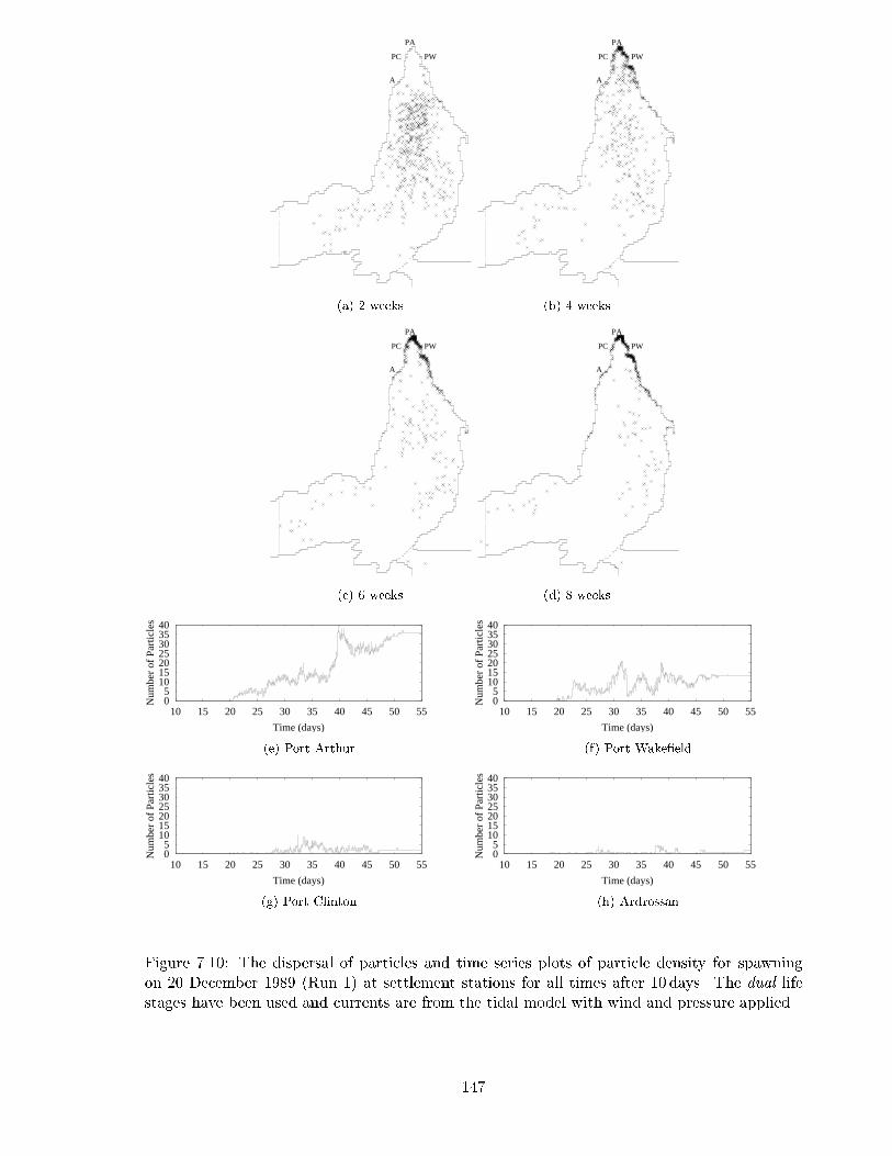
PW

PA

PC

A

(a) 2 weeks

PW

PA

PC

A

(b) 4 weeks

PW

PA

PC

A

(c) 6 weeks

PW

PA

PC

A

(d) 8 weeks

05

10152025303540

10 15 20 25 30 35 40 45 50 55

Num

ber

of P

artic

les

Time (days)

(e) Port Arthur

05

10152025303540

10 15 20 25 30 35 40 45 50 55

Num

ber

of P

artic

les

Time (days)

(f) Port Wake�eld

05

10152025303540

10 15 20 25 30 35 40 45 50 55

Num

ber

of P

artic

les

Time (days)

(g) Port Clinton

05

10152025303540

10 15 20 25 30 35 40 45 50 55

Num

ber

of P

artic

les

Time (days)

(h) Ardrossan

Figure 7.10: The dispersal of particles and time series plots of particle density for spawningon 20 December 1989 (Run 1) at settlement stations for all times after 10 days. The dual lifestages have been used and currents are from the tidal model with wind and pressure applied.

147

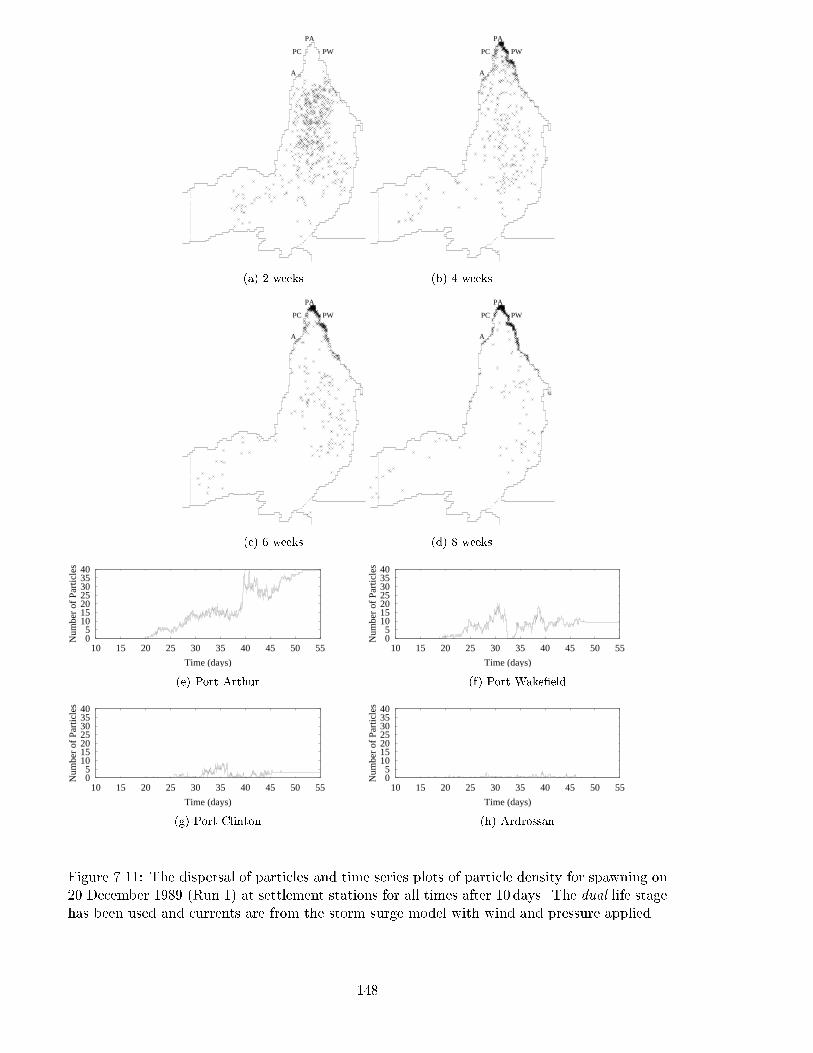
PW

PA

PC

A

(a) 2 weeks

PW

PA

PC

A

(b) 4 weeks

PW

PA

PC

A

(c) 6 weeks

PW

PA

PC

A

(d) 8 weeks

05

10152025303540

10 15 20 25 30 35 40 45 50 55

Num

ber

of P

artic

les

Time (days)

(e) Port Arthur

05

10152025303540

10 15 20 25 30 35 40 45 50 55

Num

ber

of P

artic

les

Time (days)

(f) Port Wake�eld

05

10152025303540

10 15 20 25 30 35 40 45 50 55

Num

ber

of P

artic

les

Time (days)

(g) Port Clinton

05

10152025303540

10 15 20 25 30 35 40 45 50 55

Num

ber

of P

artic

les

Time (days)

(h) Ardrossan

Figure 7.11: The dispersal of particles and time series plots of particle density for spawning on20 December 1989 (Run 1) at settlement stations for all times after 10 days. The dual life stagehas been used and currents are from the storm surge model with wind and pressure applied.

148

As expected, the dispersal of particles does not di�er signi�cantly to that when consideringtides and meteorological e�ects only. After 8 weeks high concentrations of particles are seen inthe north and north-eastern parts of the Gulf, with some settlement in the Port River Estuaryregion (see Figure 7.11(d)).

The time series plots of particle density follow a similar pattern to those previously describedwhere external surges are not included, with 39 particles at Port Arthur, 9 at Port Wake�eld,3 at Port Clinton, and 0 at Ardrossan.

7.8.2 Run 2 { settlement 1991

Tide and meteorological currents

The dual life stage scenario for western king prawn larvae is combined with tidal and mete-orological currents and applied to time period 2 in Figure 7.12.

Signi�cantly larger numbers of particles are dispersed close to the coast after 6 and 8 weeksthan when the single life stage was considered, as shown in Figures 7.12(c) and (d). There arehigh concentrations of particles at Port Arthur and Port Wake�eld, with signi�cant settlementin the region bounded by the head of the Gulf and the Port River Estuary. Almost all of theparticles have settled, with only 2 that leave the model via the open boundary.

The time series plots show signi�cant settlement of particles at Port Arthur (16 particles)and Port Wake�eld (5 particles). There is a single particle at Ardrossan, and zero at PortClinton after 55 days. Once again these are higher amounts than the densities obtained whenthe single life stage was applied.

Storm induced currents

Time period 2 is considered for prawn larvae with dual life stage behaviour and currentsobtained from tides, storm surges and meteorological e�ects in Figure 7.13.

Once again the similarity of currents when external surges are excluded to those when theyare included is obvious, as the dispersal of particles does not di�er signi�cantly between the twovelocity types. After 8 weeks (Figure 7.13(d)) the major settlement of particles occurs on thenorth-eastern coast from Port Arthur to the Port River Estuary (within which there appear tobe quite a few particles settling). This is where the major nurseries in the Gulf are known toreside. A few particles (5) have left the model via the Backstairs Passage open boundary, butmost of the particles have settled at this time.

Figures 7.13(e){(h) show that there are 17 particles that settle at Port Arthur and 12 atPort Wake�eld. No particles settle at Port Clinton or Ardrossan for this scenario.

7.9 Boundary Settlement

In order to determine the predicted positions of settlement areas, the concentration of particlesat the boundaries in the northern part of Gulf St. Vincent is considered. Various points aroundthe boundary have been assigned numerical values ranging from 1 to 100, as illustrated inFigure 7.3. It is obvious that Ardrossan is assigned point 11, Port Clinton 24, Port Arthur 28and Port Wake�eld 35. Additionally, Outer Harbor is at point number 91. For each scenarioconsidered in the previous section for the settlement of prawn larvae in the Gulf, a plot ofboundary concentration has been produced, each of which is shown in Figure 7.14.

Settlement during time period 1 is illustrated in Figures 7.14(a){(d). It is obvious thatminimal di�erences in settlement are obtained using the tide, wind and pressure induced cur-rents compared to those from the complete storm. For the single life stage there are peaks ofapproximately 20 particles at boundary points 28{35. This corresponds to Port Arthur andPort Wake�eld and the area between them. There is also a peak of particles at boundary points41{45, which corresponds to mangrove regions south of Port Wake�eld. Smaller peaks are seen

149

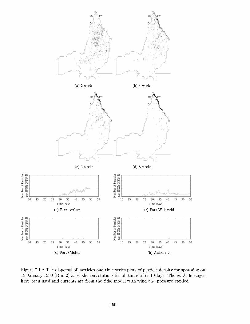
PW

PA

PC

A

(a) 2 weeks

PW

PA

PC

A

(b) 4 weeks

PW

PA

PC

A

(c) 6 weeks

PW

PA

PC

A

(d) 8 weeks

05

10152025303540

10 15 20 25 30 35 40 45 50 55

Num

ber

of P

artic

les

Time (days)

(e) Port Arthur

05

10152025303540

10 15 20 25 30 35 40 45 50 55

Num

ber

of P

artic

les

Time (days)

(f) Port Wake�eld

05

10152025303540

10 15 20 25 30 35 40 45 50 55

Num

ber

of P

artic

les

Time (days)

(g) Port Clinton

05

10152025303540

10 15 20 25 30 35 40 45 50 55

Num

ber

of P

artic

les

Time (days)

(h) Ardrossan

Figure 7.12: The dispersal of particles and time series plots of particle density for spawning on15 January 1990 (Run 2) at settlement stations for all times after 10 days. The dual life stageshave been used and currents are from the tidal model with wind and pressure applied.

150

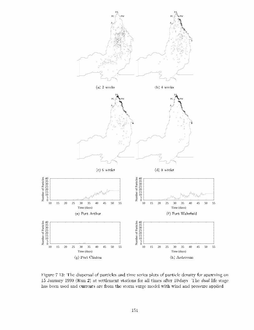
PW

PA

PC

A

(a) 2 weeks

PW

PA

PC

A

(b) 4 weeks

PW

PA

PC

A

(c) 6 weeks

PW

PA

PC

A

(d) 8 weeks

05

10152025303540

10 15 20 25 30 35 40 45 50 55

Num

ber

of P

artic

les

Time (days)

(e) Port Arthur

05

10152025303540

10 15 20 25 30 35 40 45 50 55

Num

ber

of P

artic

les

Time (days)

(f) Port Wake�eld

05

10152025303540

10 15 20 25 30 35 40 45 50 55

Num

ber

of P

artic

les

Time (days)

(g) Port Clinton

05

10152025303540

10 15 20 25 30 35 40 45 50 55

Num

ber

of P

artic

les

Time (days)

(h) Ardrossan

Figure 7.13: The dispersal of particles and time series plots of particle density for spawning on15 January 1990 (Run 2) at settlement stations for all times after 10 days. The dual life stagehas been used and currents are from the storm surge model with wind and pressure applied.

151

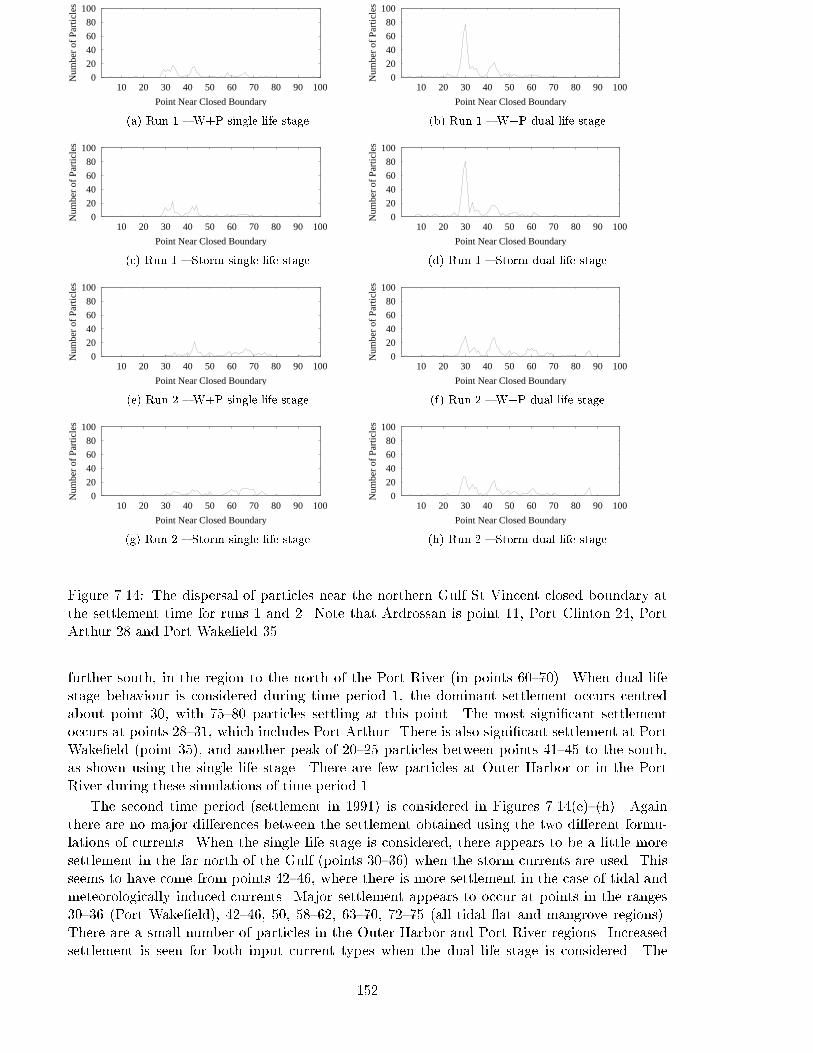
0

20

40

60

80

100

10 20 30 40 50 60 70 80 90 100

Num

ber

of P

artic

les

Point Near Closed Boundary

(a) Run 1 { W+P single life stage

0

20

40

60

80

100

10 20 30 40 50 60 70 80 90 100

Num

ber

of P

artic

les

Point Near Closed Boundary

(b) Run 1 { W+P dual life stage

0

20

40

60

80

100

10 20 30 40 50 60 70 80 90 100

Num

ber

of P

artic

les

Point Near Closed Boundary

(c) Run 1 { Storm single life stage

0

20

40

60

80

100

10 20 30 40 50 60 70 80 90 100

Num

ber

of P

artic

les

Point Near Closed Boundary

(d) Run 1 { Storm dual life stage

0

20

40

60

80

100

10 20 30 40 50 60 70 80 90 100

Num

ber

of P

artic

les

Point Near Closed Boundary

(e) Run 2 { W+P single life stage

0

20

40

60

80

100

10 20 30 40 50 60 70 80 90 100N

umbe

r of

Par

ticle

sPoint Near Closed Boundary

(f) Run 2 { W+P dual life stage

0

20

40

60

80

100

10 20 30 40 50 60 70 80 90 100

Num

ber

of P

artic

les

Point Near Closed Boundary

(g) Run 2 { Storm single life stage

0

20

40

60

80

100

10 20 30 40 50 60 70 80 90 100

Num

ber

of P

artic

les

Point Near Closed Boundary

(h) Run 2 { Storm dual life stage

Figure 7.14: The dispersal of particles near the northern Gulf St Vincent closed boundary atthe settlement time for runs 1 and 2. Note that Ardrossan is point 11, Port Clinton 24, PortArthur 28 and Port Wake�eld 35.

further south, in the region to the north of the Port River (in points 60{70). When dual lifestage behaviour is considered during time period 1, the dominant settlement occurs centredabout point 30, with 75{80 particles settling at this point. The most signi�cant settlementoccurs at points 28{31, which includes Port Arthur. There is also signi�cant settlement at PortWake�eld (point 35), and another peak of 20{25 particles between points 41{45 to the south,as shown using the single life stage. There are few particles at Outer Harbor or in the PortRiver during these simulations of time period 1.

The second time period (settlement in 1991) is considered in Figures 7.14(e){(h). Againthere are no major di�erences between the settlement obtained using the two di�erent formu-lations of currents. When the single life stage is considered, there appears to be a little moresettlement in the far north of the Gulf (points 30{36) when the storm currents are used. Thisseems to have come from points 42{46, where there is more settlement in the case of tidal andmeteorologically induced currents. Major settlement appears to occur at points in the ranges30{36 (Port Wake�eld), 42{46, 50, 58{62, 63{70, 72{75 (all tidal at and mangrove regions).There are a small number of particles in the Outer Harbor and Port River regions. Increasedsettlement is seen for both input current types when the dual life stage is considered. The

152

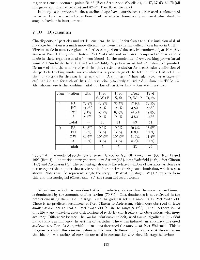
major settlement occurs at points 28{38 (Ports Arthur and Wake�eld), 40{47, 57{62, 65{70 (allmangrove and mud at regions) and 82{87 (Port River Estuary).

In many cases crevices in the coastline shape have contributed to increased settlement ofparticles. In all scenarios the settlement of particles is dramatically increased when dual lifestage behaviour is incorporated.

7.10 Discussion

The dispersal of particles and settlement near the boundaries shows that the inclusion of duallife stage behaviour is a much more e�cient way to ensure that modelled prawn larvae in Gulf St.Vincent settle in nursery regions. A further comparison of the relative numbers of particles thatsettle at Port Arthur, Port Clinton, Port Wake�eld and Ardrossan compared to observationsmade in these regions can also be considered. In the modelling of western king prawn larvaltransport conducted here, the relative mortality of prawn larvae has not been incorporated.Because of this, the number of particles that settle at a station for a particular application ofthe particle tracking model are calculated as a percentage of the total number that settle atthe four stations for that particular model run. A summary of these calculated percentages foreach station and for each of the eight scenarios previously considered is shown in Table 7.4.Also shown here is the combined total number of particles for the four stations shown.

Run Station Obs Pred Pred Pred PredS, W+P S, St D, W+P D, St

1. PA 70.8% 43.8% 36.4% 67.9% 76.5%PC 11.8% 0.0% 0.0% 3.8% 5.9%PW 9.1% 56.2% 63.6% 24.5% 17.6%A 8.3% 0.0% 0.0% 3.8% 0.0%

Total: { 16 11 53 51

2. PA 54.8% 0.0% 0.0% 69.6% 58.6%PC 0.0% 0.0% 0.0% 0.0% 0.0%PW 44.6% 100.0% 100.0% 21.7% 41.4%A 0.6% 0.0% 0.0% 8.7% 0.0%

Total: { 1 5 23 29

Table 7.4: The modelled settlement of prawn larvae for Gulf St. Vincent in 1990 (Run 1) and1991 (Run 2). The stations surveyed were Port Arthur (PA), Port Wake�eld (PW), Port Clinton(PC) and Ardrossan (A). The percentage shown is the relative number of particles written as apercentage of the number that settle at the four stations during each simulation, which is alsoshown. Note that \S" represents single life stage, \D" dual life stage, \W+P" currents fromtide and meteorological e�ects, and \St" the storm induced currents.

When time period 1 is considered, it is immediately obvious that the measured settlementis dominated by the amounts at Port Arthur (70.8%). This dominance is not re ected in thepredictions using the single life stage, with the greatest settling amounts at Port Wake�eld.There is no predicted settlement at Port Clinton or Ardrossan, which were observed to havesimilar settlement to that at Port Wake�eld (all in the range 8{12%). The incorporation ofdual life stage behaviour gives distributions of particles which re ect the observations with moreaccuracy. Di�erences between the two formulations of velocity used are not signi�cant, but tidal at activity can in uence the settling of particles. The storm induced currents have increasedsettlement at Port Arthur, which in turn has decreased the amount at Port Wake�eld. This isin agreement with the observed values at this time. Settlement only occurs at Ardrossan whenthe tide and meteorological currents are used in conjunction with dual life stage behaviour.

153

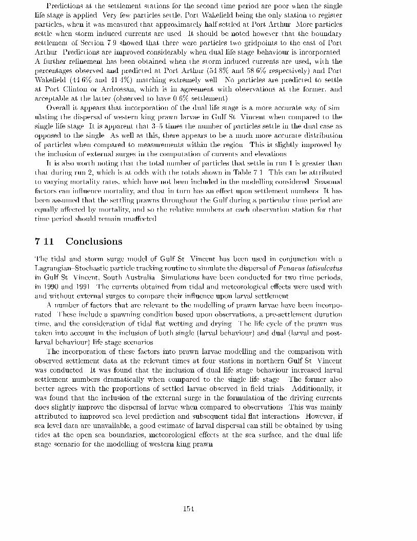
Predictions at the settlement stations for the second time period are poor when the singlelife stage is applied. Very few particles settle, Port Wake�eld being the only station to registerparticles, when it was measured that approximately half settled at Port Arthur. More particlessettle when storm induced currents are used. It should be noted however that the boundarysettlement of Section 7.9 showed that there were particles two gridpoints to the east of PortArthur. Predictions are improved considerably when dual life stage behaviour is incorporated.A further re�nement has been obtained when the storm induced currents are used, with thepercentages observed and predicted at Port Arthur (54.8% and 58.6% respectively) and PortWake�eld (44.6% and 41.4%) matching extremely well. No particles are predicted to settleat Port Clinton or Ardrossan, which is in agreement with observations at the former, andacceptable at the latter (observed to have 0.6% settlement).

Overall it appears that incorporation of the dual life stage is a more accurate way of sim-ulating the dispersal of western king prawn larvae in Gulf St. Vincent when compared to thesingle life stage. It is apparent that 3{5 times the number of particles settle in the dual case asopposed to the single. As well as this, there appears to be a much more accurate distributionof particles when compared to measurements within the region. This is slightly improved bythe inclusion of external surges in the computation of currents and elevations.

It is also worth noting that the total number of particles that settle in run 1 is greater thanthat during run 2, which is at odds with the totals shown in Table 7.1. This can be attributedto varying mortality rates, which have not been included in the modelling considered. Seasonalfactors can in uence mortality, and that in turn has an e�ect upon settlement numbers. It hasbeen assumed that the settling prawns throughout the Gulf during a particular time period areequally a�ected by mortality, and so the relative numbers at each observation station for thattime period should remain una�ected.

7.11 Conclusions

The tidal and storm surge model of Gulf St. Vincent has been used in conjunction with aLagrangian{Stochastic particle tracking routine to simulate the dispersal of Penaeus latisulcatus

in Gulf St. Vincent, South Australia. Simulations have been conducted for two time periods,in 1990 and 1991. The currents obtained from tidal and meteorological e�ects were used withand without external surges to compare their in uence upon larval settlement.

A number of factors that are relevant to the modelling of prawn larvae have been incorpo-rated. These include a spawning condition based upon observations, a pre-settlement durationtime, and the consideration of tidal at wetting and drying. The life cycle of the prawn wastaken into account in the inclusion of both single (larval behaviour) and dual (larval and post-larval behaviour) life stage scenarios.

The incorporation of these factors into prawn larvae modelling and the comparison withobserved settlement data at the relevant times at four stations in northern Gulf St. Vincentwas conducted. It was found that the inclusion of dual life stage behaviour increased larvalsettlement numbers dramatically when compared to the single life stage. The former alsobetter agrees with the proportions of settled larvae observed in �eld trials. Additionally, itwas found that the inclusion of the external surge in the formulation of the driving currentsdoes slightly improve the dispersal of larvae when compared to observations. This was mainlyattributed to improved sea level prediction and subsequent tidal at interactions. However, ifsea level data are unavailable, a good estimate of larval dispersal can still be obtained by usingtides at the open sea boundaries, meteorological e�ects at the sea surface, and the dual lifestage scenario for the modelling of western king prawn.

154

Chapter 8

Suspended Particle Dispersion in

Boston Bay, South Australia

8.1 Introduction

Boston Bay is located in the south-western part of Spencer Gulf, South Australia, adjacentto the town of Port Lincoln (see Figure 8.1). It is a shallow bay which has two entrances toSpencer Gulf, separated by Boston Island (see Figure 8.2).

Boston Bay is the site of a multi-million dollar southern blue�n tuna farming industry. In1991{1992 tuna seacage operations were established in Boston Bay as a direct result of imposedcatch limits and reduced quotas in the open sea �shery. The juvenile tuna are captured inthe seas o� southern Australia and transported to and reared in large cylindrical cages. Thesecan be up to 40m diameter (Bond, 1993) and are kept in a depth of around 15m of waterapproximately 5m from the sea oor.

In this chapter, the construction of a tidal model within Boston Bay is described. A stormsurge model of the region has subsequently been developed, and comparison with sea level andcurrent records has been conducted. Simulation of the sea levels and currents of a 1996 stormand their e�ects upon the movement of �ne organic sediment within the Bay is also investigated.Much of this work has been published by Noye et al. (1998a, 1999a), and all times are given inCentral Standard Time (CST), unless otherwise indicated.

8.2 Biology of Southern Blue�n Tuna

Southern blue�n tuna (Thunnas maccoyii) live for approximately 40 years, reaching sexualmaturity between nine and eleven years of age. A mature �sh can grow up to a length of 2m,with a weight of 200 kg. Most of the �sh caught o� of the coast of South Australia are juveniles,approximately 1.2m long with weights ranging between 15 and 30 kg.

The species have a blackish-blue upper body and silver-white lower sides and belly, with adistinctive yellow patch located about halfway along the stomach. The anal �n and �nlets areyellow, edged with black. Pectoral �ns are about one quarter to one �fth of the length of thebody, which is moderately short.

Southern blue�n eat mainly squid and octopi, crustaceans and smaller �sh, such as pilchards.They may be preyed upon by sharks, larger �sh (for example, other tuna species), sea birds,seals and killer whales at various stages of their life cycle.

These tuna can be found in southern hemisphere oceans, between 30�S and 50�S. Spawningoccurs in the warm waters of the Indian Ocean (SW of Java) from September to March. Young�sh travel south and then east around the Great Australian Bight to the South Paci�c Ocean.They tend to stay in relatively shallow coastal or shelf waters. Dispersal into the Southern,South Atlantic and Indian Oceans occurs once the tuna have matured su�ciently. Immature

155

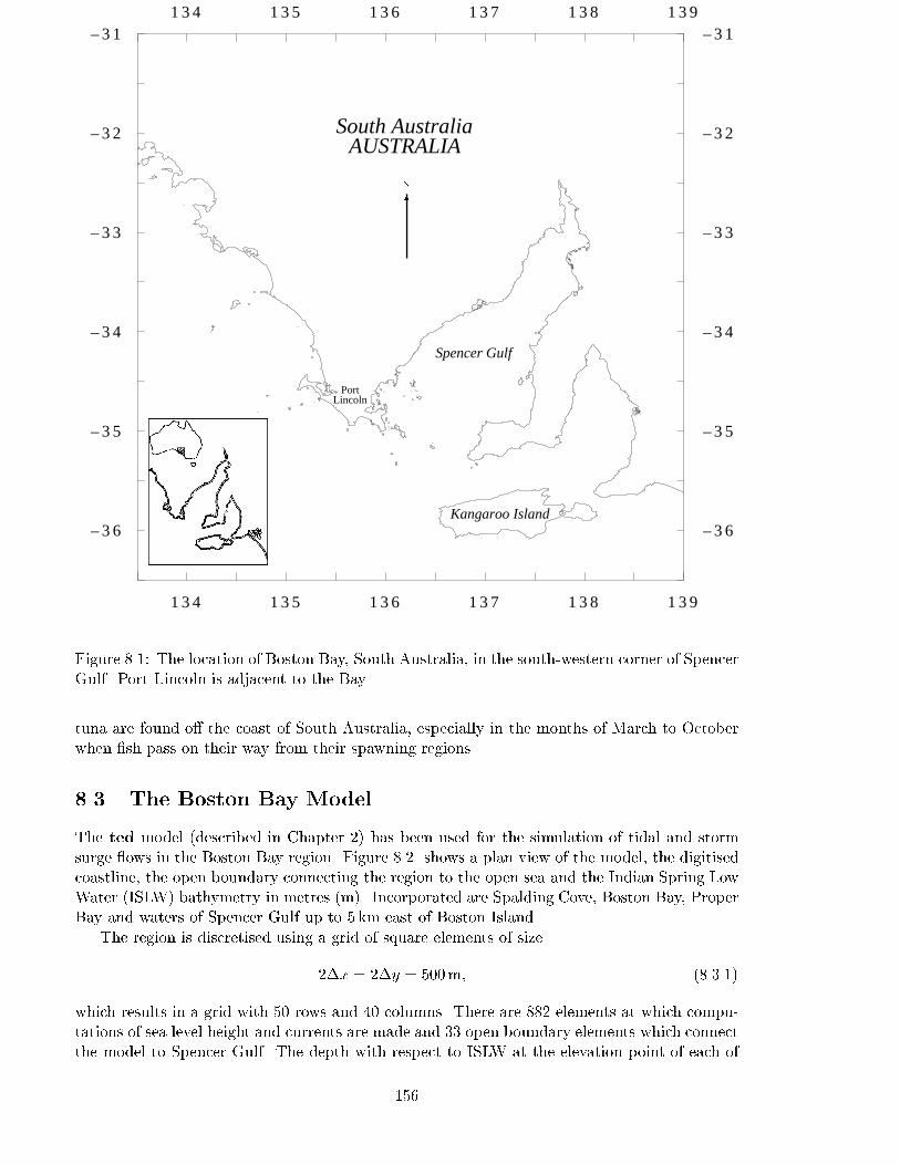
– 3 6

– 3 5

– 3 4

– 3 3

– 3 2

– 3 1

– 3 6

– 3 5

– 3 4

– 3 3

– 3 2

– 3 1

1 3 4 1 3 5 1 3 6 1 3 7 1 3 8 1 3 9

1 3 4 1 3 5 1 3 6 1 3 7 1 3 8 1 3 9

PortLincoln

Kangaroo Island

Spencer Gulf

South AustraliaAUSTRALIA

6

N

Figure 8.1: The location of Boston Bay, South Australia, in the south-western corner of SpencerGulf. Port Lincoln is adjacent to the Bay.

tuna are found o� the coast of South Australia, especially in the months of March to Octoberwhen �sh pass on their way from their spawning regions.

8.3 The Boston Bay Model

The ted model (described in Chapter 2) has been used for the simulation of tidal and stormsurge ows in the Boston Bay region. Figure 8.2 shows a plan view of the model, the digitisedcoastline, the open boundary connecting the region to the open sea and the Indian Spring LowWater (ISLW) bathymetry in metres (m). Incorporated are Spalding Cove, Boston Bay, ProperBay and waters of Spencer Gulf up to 5 km east of Boston Island.

The region is discretised using a grid of square elements of size

2�x = 2�y = 500m; (8.3.1)

which results in a grid with 50 rows and 40 columns. There are 882 elements at which compu-tations of sea level height and currents are made and 33 open boundary elements which connectthe model to Spencer Gulf. The depth with respect to ISLW at the elevation point of each of

156

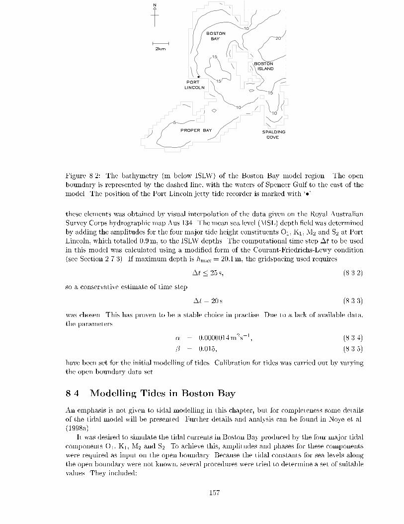
Figure 8.2: The bathymetry (m below ISLW) of the Boston Bay model region. The openboundary is represented by the dashed line, with the waters of Spencer Gulf to the east of themodel. The position of the Port Lincoln jetty tide recorder is marked with `�'.

these elements was obtained by visual interpolation of the data given on the Royal AustralianSurvey Corps hydrographic map Aus 134. The mean sea level (MSL) depth �eld was determinedby adding the amplitudes for the four major tide height constituents O1, K1, M2 and S2 at PortLincoln, which totalled 0:9m, to the ISLW depths. The computational time step �t to be usedin this model was calculated using a modi�ed form of the Courant-Friedrichs-Lewy condition(see Section 2.7.3). If maximum depth is hmax = 20:1m, the gridspacing used requires

�t � 25 s; (8.3.2)

so a conservative estimate of time step

�t = 20 s (8.3.3)

was chosen. This has proven to be a stable choice in practise. Due to a lack of available data,the parameters

� = 0:0000014m2s�1; (8.3.4)

� = 0:015; (8.3.5)

have been set for the initial modelling of tides. Calibration for tides was carried out by varyingthe open boundary data set.

8.4 Modelling Tides in Boston Bay

An emphasis is not given to tidal modelling in this chapter, but for completeness some detailsof the tidal model will be presented. Further details and analysis can be found in Noye et al.(1998a).

It was desired to simulate the tidal currents in Boston Bay produced by the four major tidalcomponents O1, K1, M2 and S2. To achieve this, amplitudes and phases for these componentswere required as input on the open boundary. Because the tidal constants for sea levels alongthe open boundary were not known, several procedures were tried to determine a set of suitablevalues. They included:

157

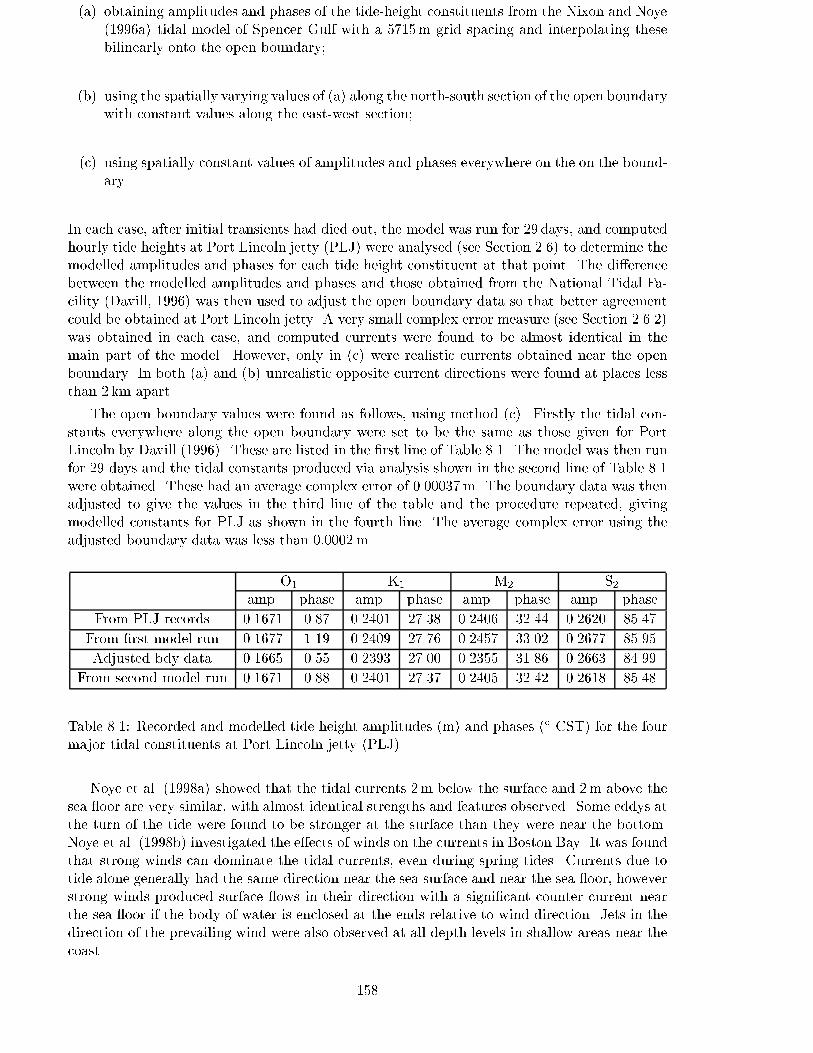
(a) obtaining amplitudes and phases of the tide-height constituents from the Nixon and Noye(1996a) tidal model of Spencer Gulf with a 5715m grid spacing and interpolating thesebilinearly onto the open boundary;

(b) using the spatially varying values of (a) along the north-south section of the open boundarywith constant values along the east-west section;

(c) using spatially constant values of amplitudes and phases everywhere on the on the bound-ary.

In each case, after initial transients had died out, the model was run for 29 days, and computedhourly tide heights at Port Lincoln jetty (PLJ) were analysed (see Section 2.6) to determine themodelled amplitudes and phases for each tide height constituent at that point. The di�erencebetween the modelled amplitudes and phases and those obtained from the National Tidal Fa-cility (Davill, 1996) was then used to adjust the open boundary data so that better agreementcould be obtained at Port Lincoln jetty. A very small complex error measure (see Section 2.6.2)was obtained in each case, and computed currents were found to be almost identical in themain part of the model. However, only in (c) were realistic currents obtained near the openboundary. In both (a) and (b) unrealistic opposite current directions were found at places lessthan 2 km apart.

The open boundary values were found as follows, using method (c). Firstly the tidal con-stants everywhere along the open boundary were set to be the same as those given for PortLincoln by Davill (1996). These are listed in the �rst line of Table 8.1. The model was then runfor 29 days and the tidal constants produced via analysis shown in the second line of Table 8.1were obtained. These had an average complex error of 0.00037m. The boundary data was thenadjusted to give the values in the third line of the table and the procedure repeated, givingmodelled constants for PLJ as shown in the fourth line. The average complex error using theadjusted boundary data was less than 0:0002m.

O1 K1 M2 S2amp. phase amp. phase amp. phase amp. phase

From PLJ records 0.1671 0.87 0.2401 27.38 0.2406 32.44 0.2620 85.47

From �rst model run 0.1677 1.19 0.2409 27.76 0.2457 33.02 0.2677 85.95

Adjusted bdy data 0.1665 0.55 0.2393 27.00 0.2355 31.86 0.2663 84.99

From second model run 0.1671 0.88 0.2401 27.37 0.2405 32.42 0.2618 85.48

Table 8.1: Recorded and modelled tide height amplitudes (m) and phases (� CST) for the fourmajor tidal constituents at Port Lincoln jetty (PLJ).

Noye et al. (1998a) showed that the tidal currents 2m below the surface and 2m above thesea oor are very similar, with almost identical strengths and features observed. Some eddys atthe turn of the tide were found to be stronger at the surface than they were near the bottom.Noye et al. (1998b) investigated the e�ects of winds on the currents in Boston Bay. It was foundthat strong winds can dominate the tidal currents, even during spring tides. Currents due totide alone generally had the same direction near the sea surface and near the sea oor, howeverstrong winds produced surface ows in their direction with a signi�cant counter current nearthe sea oor if the body of water is enclosed at the ends relative to wind direction. Jets in thedirection of the prevailing wind were also observed at all depth levels in shallow areas near thecoast.

158

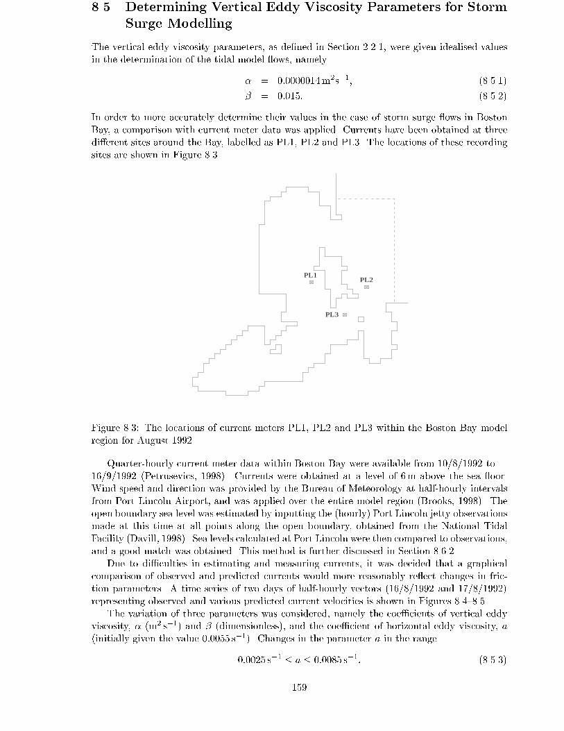
8.5 Determining Vertical Eddy Viscosity Parameters for Storm

Surge Modelling

The vertical eddy viscosity parameters, as de�ned in Section 2.2.1, were given idealised valuesin the determination of the tidal model ows, namely

� = 0:0000014m2s�1; (8.5.1)

� = 0:015: (8.5.2)

In order to more accurately determine their values in the case of storm surge ows in BostonBay, a comparison with current meter data was applied. Currents have been obtained at threedi�erent sites around the Bay, labelled as PL1, PL2 and PL3. The locations of these recordingsites are shown in Figure 8.3.

PL1PL2

PL3

Figure 8.3: The locations of current meters PL1, PL2 and PL3 within the Boston Bay modelregion for August 1992.

Quarter-hourly current meter data within Boston Bay were available from 10/8/1992 to16/9/1992 (Petrusevics, 1998). Currents were obtained at a level of 6m above the sea oor.Wind speed and direction was provided by the Bureau of Meteorology at half-hourly intervalsfrom Port Lincoln Airport, and was applied over the entire model region (Brooks, 1998). Theopen boundary sea level was estimated by inputting the (hourly) Port Lincoln jetty observationsmade at this time at all points along the open boundary, obtained from the National TidalFacility (Davill, 1998). Sea levels calculated at Port Lincoln were then compared to observations,and a good match was obtained. This method is further discussed in Section 8.6.2.

Due to di�culties in estimating and measuring currents, it was decided that a graphicalcomparison of observed and predicted currents would more reasonably re ect changes in fric-tion parameters. A time series of two days of half-hourly vectors (16/8/1992 and 17/8/1992)representing observed and various predicted current velocities is shown in Figures 8.4{8.5.

The variation of three parameters was considered, namely the coe�cients of vertical eddyviscosity, � (m2 s�1) and � (dimensionless), and the coe�cient of horizontal eddy viscosity, a(initially given the value 0:0055 s�1). Changes in the parameter a in the range

0:0025 s�1 � a � 0:0085 s�1; (8.5.3)

159

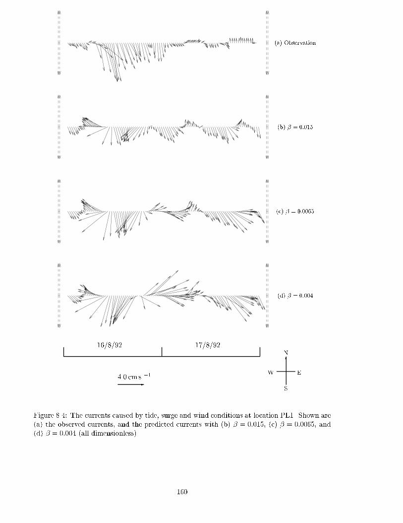
(a) Observation

(b) � = 0:015

(c) � = 0:0065

(d) � = 0:004

16/8/92 17/8/92

4.0 cm s �1

-

N

S

EW

6

Figure 8.4: The currents caused by tide, surge and wind conditions at location PL1. Shown are(a) the observed currents, and the predicted currents with (b) � = 0:015, (c) � = 0:0065, and(d) � = 0:004 (all dimensionless).

160

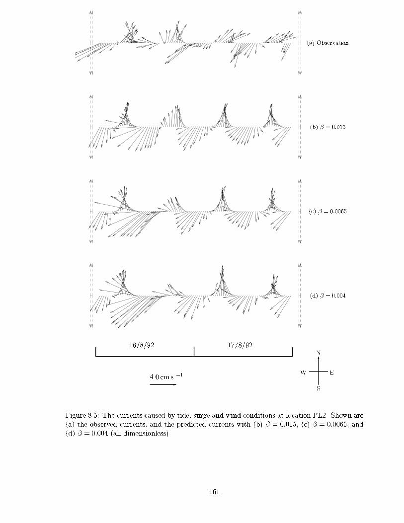
(a) Observation

(b) � = 0:015

(c) � = 0:0065

(d) � = 0:004

16/8/92 17/8/92

4.0 cm s �1

-

N

S

EW

6

Figure 8.5: The currents caused by tide, surge and wind conditions at location PL2. Shown are(a) the observed currents, and the predicted currents with (b) � = 0:015, (c) � = 0:0065, and(d) � = 0:004 (all dimensionless).

161

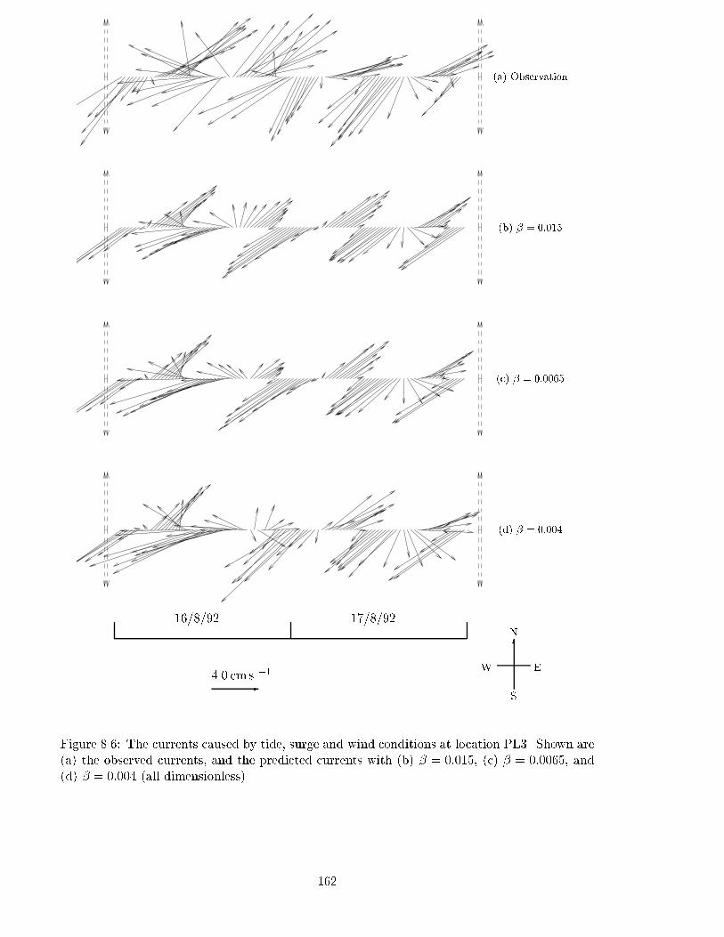
(a) Observation

(b) � = 0:015

(c) � = 0:0065

(d) � = 0:004

16/8/92 17/8/92

4.0 cm s �1

-

N

S

EW

6

Figure 8.6: The currents caused by tide, surge and wind conditions at location PL3. Shown are(a) the observed currents, and the predicted currents with (b) � = 0:015, (c) � = 0:0065, and(d) � = 0:004 (all dimensionless).

162

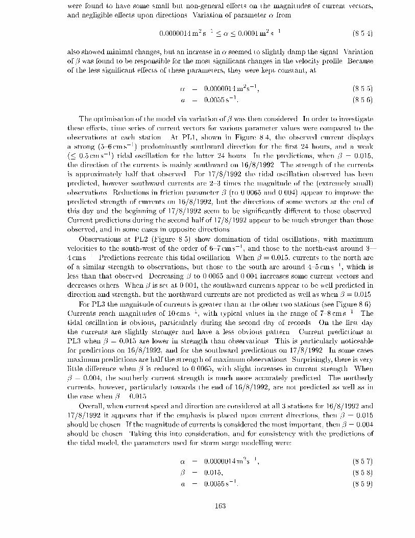
were found to have some small but non-general e�ects on the magnitudes of current vectors,and negligible e�ects upon directions. Variation of parameter � from

0:0000014m2 s�1 � � � 0:0001m2 s�1 (8.5.4)

also showed minimal changes, but an increase in � seemed to slightly damp the signal. Variationof � was found to be responsible for the most signi�cant changes in the velocity pro�le. Becauseof the less signi�cant e�ects of these parameters, they were kept constant, at

� = 0:0000014m2s�1; (8.5.5)

a = 0:0055 s�1: (8.5.6)

The optimisation of the model via variation of � was then considered. In order to investigatethese e�ects, time series of current vectors for various parameter values were compared to theobservations at each station. At PL1, shown in Figure 8.4, the observed current displaysa strong (5{6 cm s�1) predominantly southward direction for the �rst 24 hours, and a weak(� 0:5 cm s�1) tidal oscillation for the latter 24 hours. In the predictions, when � = 0:015,the direction of the currents is mainly southward on 16/8/1992. The strength of the currentsis approximately half that observed. For 17/8/1992 the tidal oscillation observed has beenpredicted, however southward currents are 2{3 times the magnitude of the (extremely small)observations. Reductions in friction parameter � (to 0.0065 and 0.004) appear to improve thepredicted strength of currents on 16/8/1992, but the directions of some vectors at the end ofthis day and the beginning of 17/8/1992 seem to be signi�cantly di�erent to those observed.Current predictions during the second half of 17/8/1992 appear to be much stronger than thoseobserved, and in some cases in opposite directions.

Observations at PL2 (Figure 8.5) show domination of tidal oscillations, with maximumvelocities to the south-west of the order of 6{7 cm s�1, and those to the north-east around 3{4 cm s�1. Predictions recreate this tidal oscillation. When � = 0:015, currents to the north areof a similar strength to observations, but those to the south are around 4{5 cm s�1, which isless than that observed. Decreasing � to 0.0065 and 0.004 increases some current vectors anddecreases others. When � is set at 0.004, the southward currents appear to be well predicted indirection and strength, but the northward currents are not predicted as well as when � = 0:015.

For PL3 the magnitude of currents is greater than at the other two stations (see Figure 8.6).Currents reach magnitudes of 10 cm s�1, with typical values in the range of 7{8 cm s�1. Thetidal oscillation is obvious, particularly during the second day of records. On the �rst daythe currents are slightly stronger and have a less obvious pattern. Current predictions atPL3 when � = 0:015 are lower in strength than observations. This is particularly noticeablefor predictions on 16/8/1992, and for the southward predictions on 17/8/1992. In some casesmaximum predictions are half the strength of maximum observations. Surprisingly, there is verylittle di�erence when � is reduced to 0.0065, with slight increases in current strength. When� = 0:004, the southerly current strength is much more accurately predicted. The northerlycurrents, however, particularly towards the end of 16/8/1992, are not predicted as well as inthe case when � = 0:015.

Overall, when current speed and direction are considered at all 3 stations for 16/8/1992 and17/8/1992 it appears that if the emphasis is placed upon current directions, then � = 0:015should be chosen. If the magnitude of currents is considered the most important, then � = 0:004should be chosen. Taking this into consideration, and for consistency with the predictions ofthe tidal model, the parameters used for storm surge modelling were:

� = 0:0000014m2s�1; (8.5.7)

� = 0:015; (8.5.8)

a = 0:0055 s�1: (8.5.9)

163

8.6 The Disaster of April 1996

On Tuesday 16 April 1996, the South Australian Government was noti�ed that, from 13 April 1996,abnormal mortalities of southern blue�n tuna had occurred in the tuna research farm and com-mercial tuna farms in Boston Bay. Excessive mortalities continued over the next two to threeweeks, with an estimated 1700 tonnes of tuna, three-quarters of the stock in the farms, dyingduring this period (Clarke, 1996).

As a result of this disaster, a working group commissioned by the South Australian Gov-ernment was formed to investigate and report on the causes of these mortalities. Based on anassessment of data and information collected on meteorological and oceanographic conditions,water quality, water chemistry, micro algae, mussel toxicology, �sh pathology and microbiology,potential causes such as micro algae were eliminated (Clarke, 1996).

The most probable cause of the abnormal mortalities was an unusual meteorological eventon 11{12 April 1996, when a storm associated with the remnants of tropical cyclone OLIVIAtravelled east-southeast across the Great Australian Bight (as simulated in Chapter 5) andpassed over Port Lincoln, producing strong winds from the north-east for approximately 12 hours(see Figure 8.7(a)).

These strong winds persisted over the long fetch of water in the north-easterly direction alongthe axis of Spencer Gulf (approximately 350 km) producing wind waves of su�cient energyto lift �ne almost neutrally buoyant organic sediments o� the sea oor and into suspension(Petrusevics, 1996; Walker, 1996). These sediments were thought to have coated the gills of the�sh, causing trauma and death from su�ocation within 3{5 days. It is notable that a storm ofequivalent severity also occurred at Port Lincoln on 15{19 October 1995 but this did not resultin abnormal tuna mortalities. The winds that persisted during this event were predominantlyfrom the north-west (see Figure 8.7(b)). The fetch of water is very short in this direction, sothat wind waves produced did not have su�cient energy to disturb the bottom sediments inthe Bay.

8.6.1 The tuna mortalities

Data on the tuna mortalities was obtained for the period 13{30 April 1996, from the TunaBoat Owners Association of Australia (TBOAA, 1997). Throughout this time there were oftenlengthy periods where it appeared that no deaths had occurred, followed by a large number ofdeaths recorded on one particular day. This was found to be due to the irregular frequency ofmortality counts, where no deaths were registered for several days followed by a sudden largeincrease in the number of deaths recorded. In such cases, the increment was spread uniformlyover the previous days of no recorded mortalities.

Eight tuna farm locations, denoted A{H as shown in Figure 8.8, were identi�ed and thedata from all the farms in each of these locations collated. Percentages of daily and cumulativedeaths were then determined from stock totals at 12/4/1996. The results from these calculationsare shown in Figures 8.9 and 8.10, which give the percentage daily deaths and the percentagecumulative deaths respectively at the eight locations around Boston Island.

Graphs of daily tuna mortalities (Figure 8.9) show that in the �rst week following the storm,farms to the north-west and south of Boston Island (i.e. at A, C and D) su�ered the greatestlosses, with mortalities at G (to the east) slightly less than these. Farms north-east, south-eastand west of Boston Island (i.e. at H, F and B) as well as to the north-east of Bickers Islands(i.e. at E) were not a�ected as much in the �rst seven days. After this time, there was anincrease in mortality rates at G and B, with the most signi�cant single loss observed at C (16%on 23/4/1996). For locations H and F low mortalities were probably due to the fact that farmsat H were moved from this area between 15/4/1996 and 17/4/1996, and F left the area on16/4/1996. Farm D was moved on 23/4/1996, after which mortalities at this location slowed.This, along with the relatively small losses obtained at E (which was not moved) suggests thatthe location of the farms tends to be the determining factor for the number of mortalities. It

164

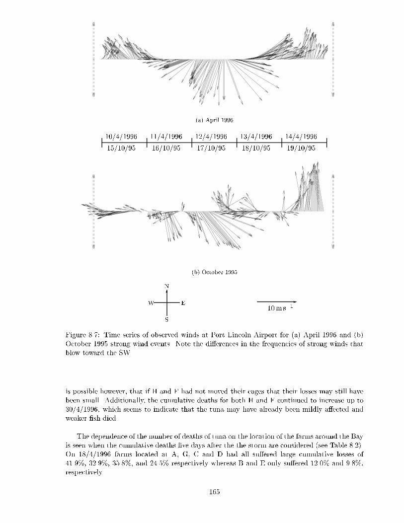
(a) April 1996

10/4/1996 11/4/1996 12/4/1996 13/4/1996 14/4/1996

15/10/95 16/10/95 17/10/95 18/10/95 19/10/95

(b) October 1995

N

S

EW

6-

10m s�1

Figure 8.7: Time series of observed winds at Port Lincoln Airport for (a) April 1996 and (b)October 1995 strong wind events. Note the di�erences in the frequencies of strong winds thatblow toward the SW.

is possible however, that if H and F had not moved their cages that their losses may still havebeen small. Additionally, the cumulative deaths for both H and F continued to increase up to30/4/1996, which seems to indicate that the tuna may have already been mildly a�ected andweaker �sh died.

The dependence of the number of deaths of tuna on the location of the farms around the Bayis seen when the cumulative deaths �ve days after the the storm are considered (see Table 8.2).On 18/4/1996 farms located at A, G, C and D had all su�ered large cumulative losses of41.9%, 32.9%, 35.8%, and 24.5% respectively whereas B and E only su�ered 12.0% and 9.8%,respectively.

165

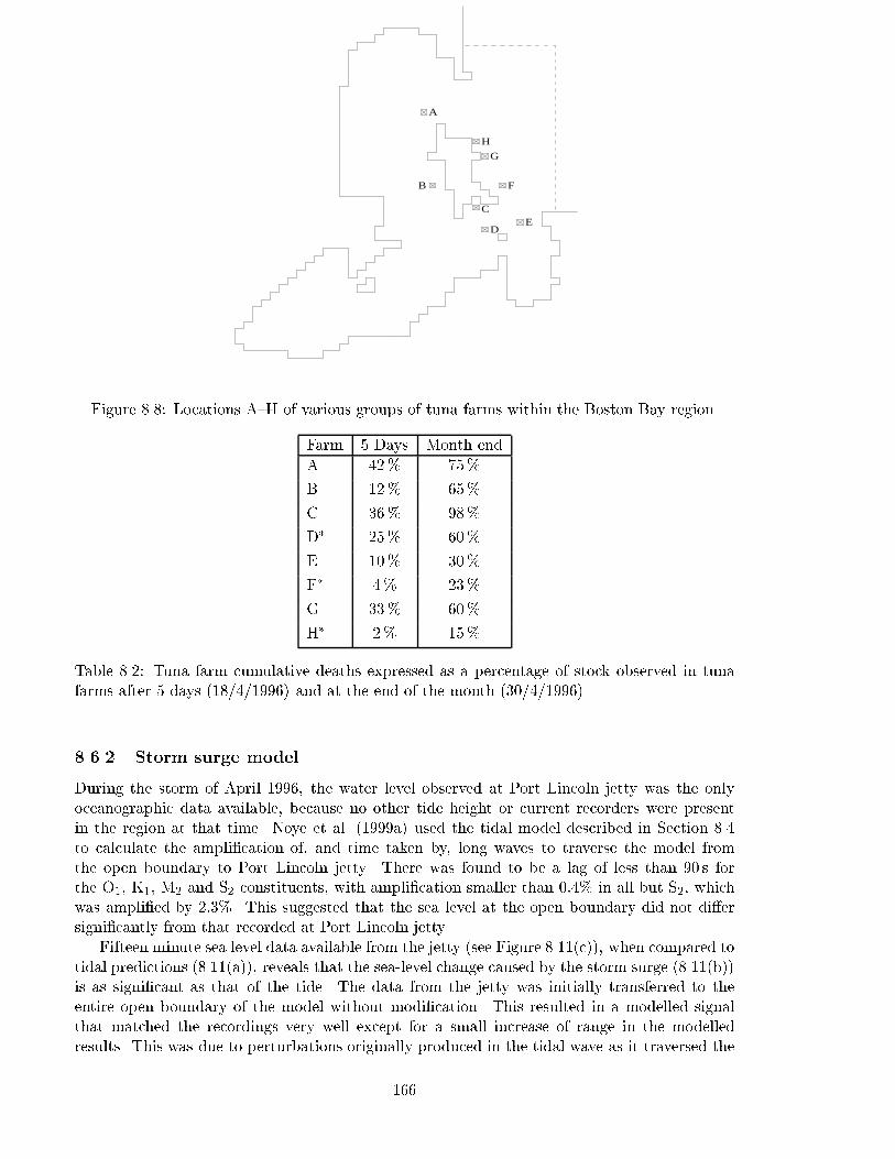
A

B

C

DE

F

G

H

Figure 8.8: Locations A{H of various groups of tuna farms within the Boston Bay region.

Farm 5 Days Month end

A 42% 75%

B 12% 65%

C 36% 98%

D� 25% 60%

E 10% 30%

F� 4% 23%

G 33% 60%

H� 2% 15%

Table 8.2: Tuna farm cumulative deaths expressed as a percentage of stock observed in tunafarms after 5 days (18/4/1996) and at the end of the month (30/4/1996).

8.6.2 Storm surge model

During the storm of April 1996, the water level observed at Port Lincoln jetty was the onlyoceanographic data available, because no other tide height or current recorders were presentin the region at that time. Noye et al. (1999a) used the tidal model described in Section 8.4to calculate the ampli�cation of, and time taken by, long waves to traverse the model fromthe open boundary to Port Lincoln jetty. There was found to be a lag of less than 90 s forthe O1, K1, M2 and S2 constituents, with ampli�cation smaller than 0:4% in all but S2, whichwas ampli�ed by 2:3%. This suggested that the sea level at the open boundary did not di�ersigni�cantly from that recorded at Port Lincoln jetty.

Fifteen minute sea level data available from the jetty (see Figure 8.11(c)), when compared totidal predictions (8.11(a)), reveals that the sea-level change caused by the storm surge (8.11(b))is as signi�cant as that of the tide. The data from the jetty was initially transferred to theentire open boundary of the model without modi�cation. This resulted in a modelled signalthat matched the recordings very well except for a small increase of range in the modelledresults. This was due to perturbations originally produced in the tidal wave as it traversed the

166

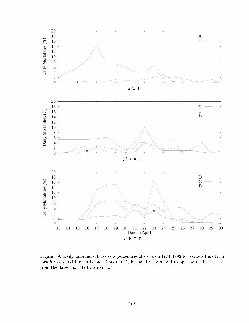
02468

101214161820

Dai

ly M

orta

litie

s (%

)

x

AH

(a) A, H

02468

101214161820

Dai

ly M

orta

litie

s (%

)

x

GFE

(b) E, F, G

02468

101214161820

13 14 15 16 17 18 19 20 21 22 23 24 25 26 27 28 29 30

Dai

ly M

orta

litie

s (%

)

Date in April

x

DCB

(c) B, C, D

Figure 8.9: Daily tuna mortalities as a percentage of stock on 12/4/1996 for various tuna farmlocations around Boston Island. Cages at D, F and H were moved to open water in the eastfrom the dates indicated with an \x".

167

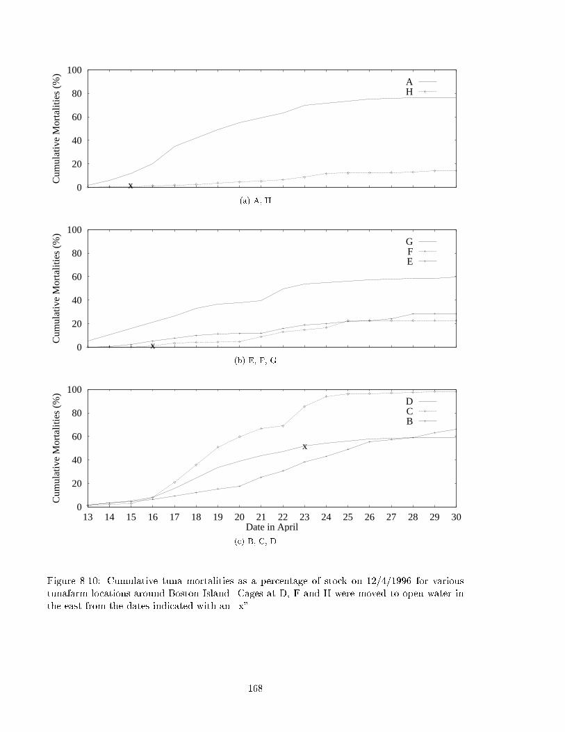
0

20

40

60

80

100

Cum

ulat

ive

Mor

talit

ies

(%)

x

AH

(a) A, H

0

20

40

60

80

100

Cum

ulat

ive

Mor

talit

ies

(%)

x

GFE

(b) E, F, G

0

20

40

60

80

100

13 14 15 16 17 18 19 20 21 22 23 24 25 26 27 28 29 30

Cum

ulat

ive

Mor

talit

ies

(%)

Date in April

x

DCB

(c) B, C, D

Figure 8.10: Cumulative tuna mortalities as a percentage of stock on 12/4/1996 for varioustunafarm locations around Boston Island. Cages at D, F and H were moved to open water inthe east from the dates indicated with an \x".

168

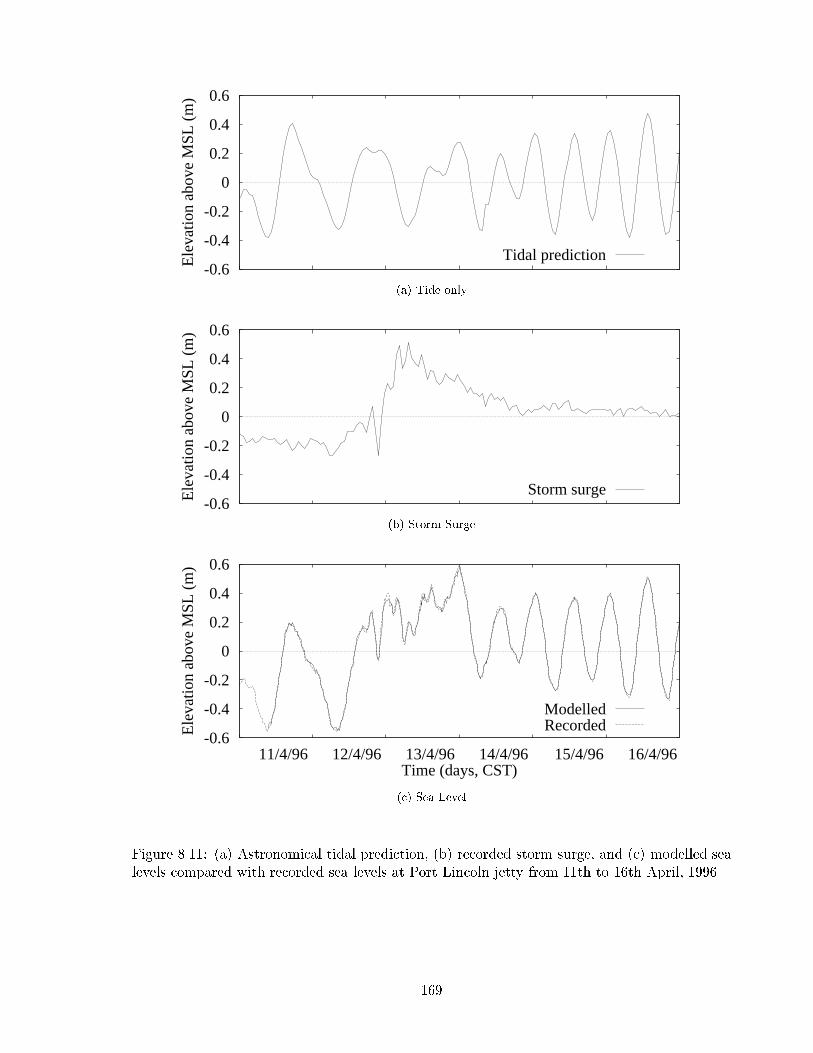
-0.6

-0.4

-0.2

0

0.2

0.4

0.6

Ele

vatio

n ab

ove

MSL

(m

)

Tidal prediction

(a) Tide only

-0.6

-0.4

-0.2

0

0.2

0.4

0.6

Ele

vatio

n ab

ove

MSL

(m

)

Storm surge

(b) Storm Surge

-0.6

-0.4

-0.2

0

0.2

0.4

0.6

11/4/96 12/4/96 13/4/96 14/4/96 15/4/96 16/4/96

Ele

vatio

n ab

ove

MSL

(m

)

Time (days, CST)

ModelledRecorded

(c) Sea Level

Figure 8.11: (a) Astronomical tidal prediction, (b) recorded storm surge, and (c) modelled sealevels compared with recorded sea levels at Port Lincoln jetty from 11th to 16th April, 1996.

169

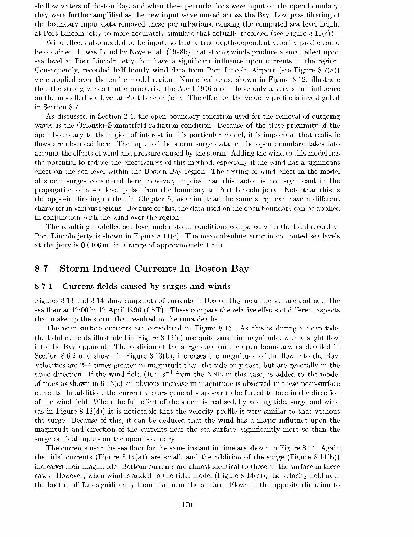
shallow waters of Boston Bay, and when these perturbations were input on the open boundary,they were further ampli�ed as the new input wave moved across the Bay. Low pass �ltering ofthe boundary input data removed these perturbations, causing the computed sea level heightat Port Lincoln jetty to more accurately simulate that actually recorded (see Figure 8.11(c)).

Wind e�ects also needed to be input, so that a true depth-dependent velocity pro�le couldbe obtained. It was found by Noye et al. (1998b) that strong winds produce a small e�ect uponsea level at Port Lincoln jetty, but have a signi�cant in uence upon currents in the region.Consequently, recorded half hourly wind data from Port Lincoln Airport (see Figure 8.7(a))were applied over the entire model region. Numerical tests, shown in Figure 8.12, illustratethat the strong winds that characterise the April 1996 storm have only a very small in uenceon the modelled sea level at Port Lincoln jetty. The e�ect on the velocity pro�le is investigatedin Section 8.7.

As discussed in Section 2.4, the open boundary condition used for the removal of outgoingwaves is the Orlanski{Sommerfeld radiation condition. Because of the close proximity of theopen boundary to the region of interest in this particular model, it is important that realistic ows are observed here. The input of the storm surge data on the open boundary takes intoaccount the e�ects of wind and pressure caused by the storm. Adding the wind to this model hasthe potential to reduce the e�ectiveness of this method, especially if the wind has a signi�cante�ect on the sea level within the Boston Bay region. The testing of wind e�ect in the modelof storm surges considered here, however, implies that this factor is not signi�cant in thepropagation of a sea level pulse from the boundary to Port Lincoln jetty. Note that this isthe opposite �nding to that in Chapter 5, meaning that the same surge can have a di�erentcharacter in various regions. Because of this, the data used on the open boundary can be appliedin conjunction with the wind over the region.

The resulting modelled sea level under storm conditions compared with the tidal record atPort Lincoln jetty is shown in Figure 8.11(c). The mean absolute error in computed sea levelsat the jetty is 0:0106m, in a range of approximately 1:5m.

8.7 Storm Induced Currents In Boston Bay

8.7.1 Current �elds caused by surges and winds

Figures 8.13 and 8.14 show snapshots of currents in Boston Bay near the surface and near thesea oor at 12:00 hr 12 April 1996 (CST). These compare the relative e�ects of di�erent aspectsthat make up the storm that resulted in the tuna deaths.

The near surface currents are considered in Figure 8.13. As this is during a neap tide,the tidal currents illustrated in Figure 8.13(a) are quite small in magnitude, with a slight owinto the Bay apparent. The addition of the surge data on the open boundary, as detailed inSection 8.6.2 and shown in Figure 8.13(b), increases the magnitude of the ow into the Bay.Velocities are 2{4 times greater in magnitude than the tide only case, but are generally in thesame direction. If the wind �eld (10m s�1 from the NNE in this case) is added to the modelof tides as shown in 8.13(c) an obvious increase in magnitude is observed in these near-surfacecurrents. In addition, the current vectors generally appear to be forced to face in the directionof the wind �eld. When the full e�ect of the storm is realised, by adding tide, surge and wind(as in Figure 8.13(d)) it is noticeable that the velocity pro�le is very similar to that withoutthe surge. Because of this, it can be deduced that the wind has a major in uence upon themagnitude and direction of the currents near the sea surface, signi�cantly more so than thesurge or tidal inputs on the open boundary.

The currents near the sea oor for the same instant in time are shown in Figure 8.14. Againthe tidal currents (Figure 8.14(a)) are small, and the addition of the surge (Figure 8.14(b))increases their magnitude. Bottom currents are almost identical to those at the surface in thesecases. However, when wind is added to the tidal model (Figure 8.14(c)), the velocity �eld nearthe bottom di�ers signi�cantly from that near the surface. Flows in the opposite direction to

170

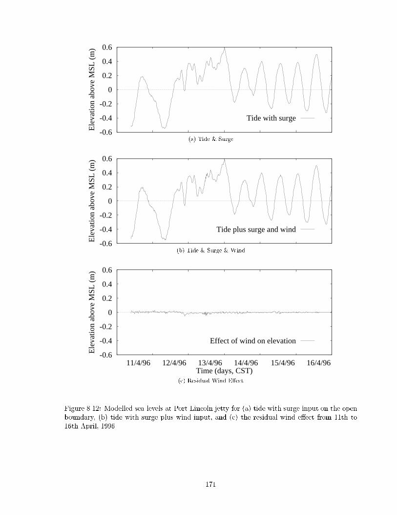
-0.6

-0.4

-0.2

0

0.2

0.4

0.6

Ele

vatio

n ab

ove

MSL

(m

)

Tide with surge

(a) Tide & Surge

-0.6

-0.4

-0.2

0

0.2

0.4

0.6

Ele

vatio

n ab

ove

MSL

(m

)

Tide plus surge and wind

(b) Tide & Surge & Wind

-0.6

-0.4

-0.2

0

0.2

0.4

0.6

11/4/96 12/4/96 13/4/96 14/4/96 15/4/96 16/4/96

Ele

vatio

n ab

ove

MSL

(m

)

Time (days, CST)

Effect of wind on elevation

(c) Residual Wind E�ect

Figure 8.12: Modelled sea levels at Port Lincoln jetty for (a) tide with surge input on the openboundary, (b) tide with surge plus wind input, and (c) the residual wind e�ect from 11th to16th April, 1996.

171

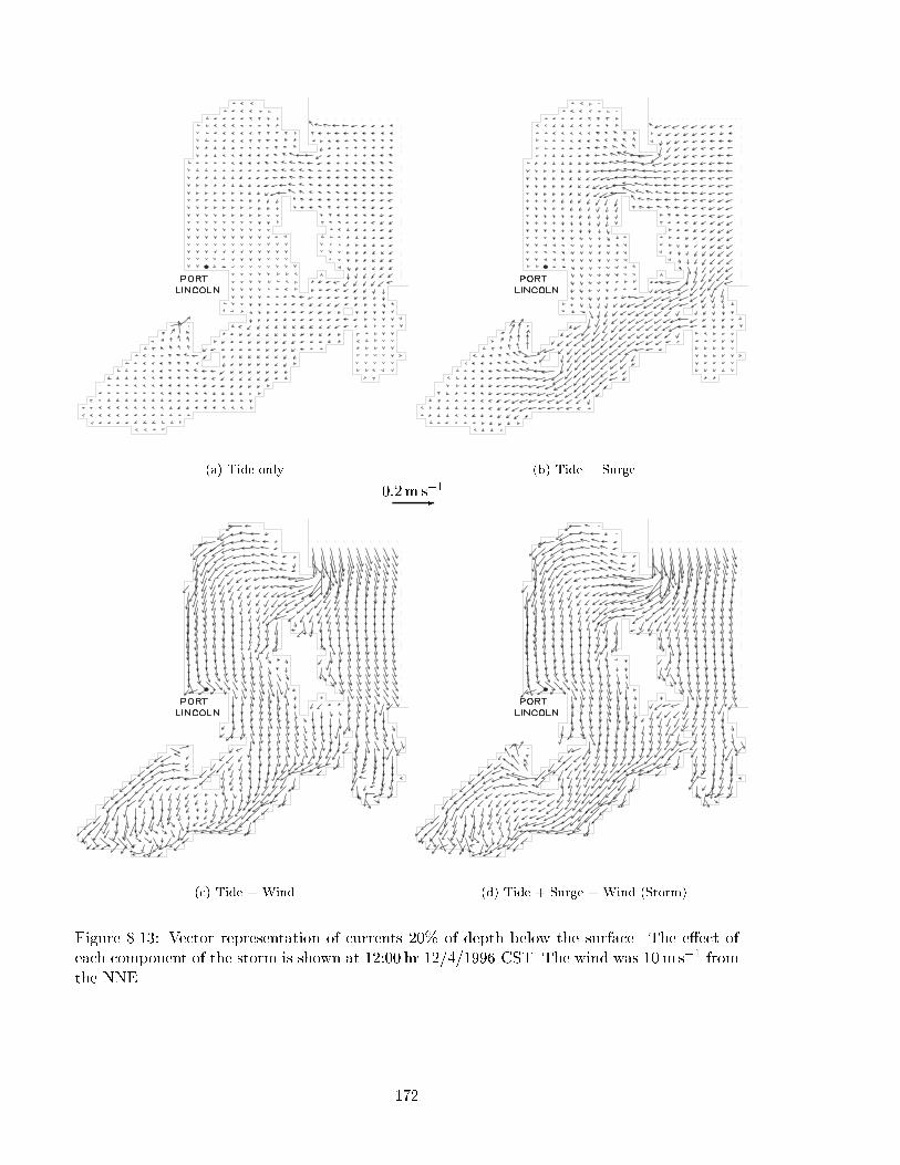
(a) Tide only (b) Tide + Surge

0:2m s�1-

(c) Tide + Wind (d) Tide + Surge + Wind (Storm)

Figure 8.13: Vector representation of currents 20% of depth below the surface. The e�ect ofeach component of the storm is shown at 12:00 hr 12/4/1996 CST. The wind was 10ms�1 fromthe NNE.

172

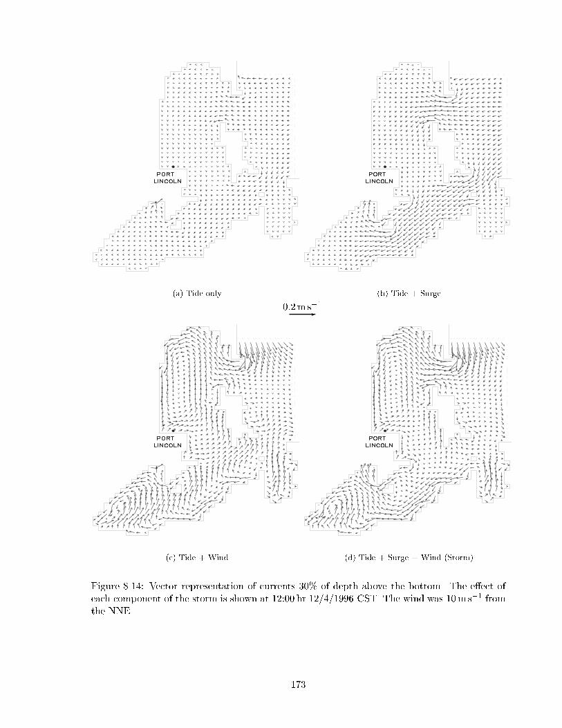
(a) Tide only (b) Tide + Surge

0:2m s�1-

(c) Tide + Wind (d) Tide + Surge + Wind (Storm)

Figure 8.14: Vector representation of currents 30% of depth above the bottom. The e�ect ofeach component of the storm is shown at 12:00 hr 12/4/1996 CST. The wind was 10m s�1 fromthe NNE.

173

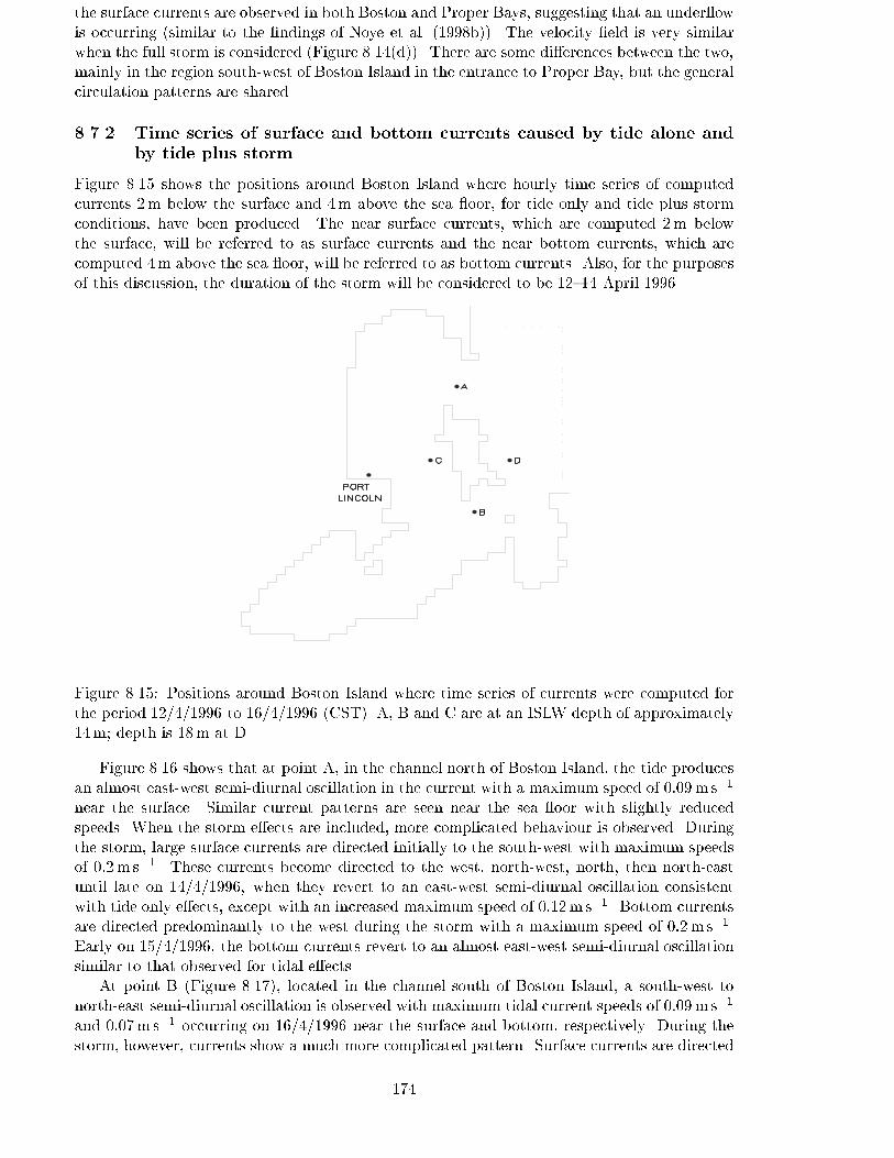
the surface currents are observed in both Boston and Proper Bays, suggesting that an under owis occurring (similar to the �ndings of Noye et al. (1998b)). The velocity �eld is very similarwhen the full storm is considered (Figure 8.14(d)). There are some di�erences between the two,mainly in the region south-west of Boston Island in the entrance to Proper Bay, but the generalcirculation patterns are shared.

8.7.2 Time series of surface and bottom currents caused by tide alone and

by tide plus storm

Figure 8.15 shows the positions around Boston Island where hourly time series of computedcurrents 2m below the surface and 4m above the sea oor, for tide only and tide plus stormconditions, have been produced. The near surface currents, which are computed 2m belowthe surface, will be referred to as surface currents and the near bottom currents, which arecomputed 4m above the sea oor, will be referred to as bottom currents. Also, for the purposesof this discussion, the duration of the storm will be considered to be 12{14 April 1996.

Figure 8.15: Positions around Boston Island where time series of currents were computed forthe period 12/4/1996 to 16/4/1996 (CST). A, B and C are at an ISLW depth of approximately14m; depth is 18m at D.

Figure 8.16 shows that at point A, in the channel north of Boston Island, the tide producesan almost east-west semi-diurnal oscillation in the current with a maximum speed of 0:09m s�1

near the surface. Similar current patterns are seen near the sea oor with slightly reducedspeeds. When the storm e�ects are included, more complicated behaviour is observed. Duringthe storm, large surface currents are directed initially to the south-west with maximum speedsof 0:2m s�1. These currents become directed to the west, north-west, north, then north-eastuntil late on 14/4/1996, when they revert to an east-west semi-diurnal oscillation consistentwith tide only e�ects, except with an increased maximum speed of 0:12m s�1. Bottom currentsare directed predominantly to the west during the storm with a maximum speed of 0:2m s�1.Early on 15/4/1996, the bottom currents revert to an almost east-west semi-diurnal oscillationsimilar to that observed for tidal e�ects.

At point B (Figure 8.17), located in the channel south of Boston Island, a south-west tonorth-east semi-diurnal oscillation is observed with maximum tidal current speeds of 0:09m s�1

and 0:07m s�1 occurring on 16/4/1996 near the surface and bottom, respectively. During thestorm, however, currents show a much more complicated pattern. Surface currents are directed

174

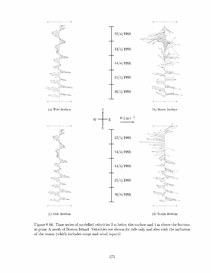
(a) Tide Surface

12/4/1996

13/4/1996

14/4/1996

15/4/1996

16/4/1996

(b) Storm Surface

0.1m s�1-

N

S

EW

66

(c) Tide Bottom

12/4/1996

13/4/1996

14/4/1996

15/4/1996

16/4/1996

(d) Storm Bottom

Figure 8.16: Time series of modelled velocities 2m below the surface and 4m above the bottomat point A north of Boston Island. Velocities are shown for tide only and also with the inclusionof the storm (which includes surge and wind inputs).

175

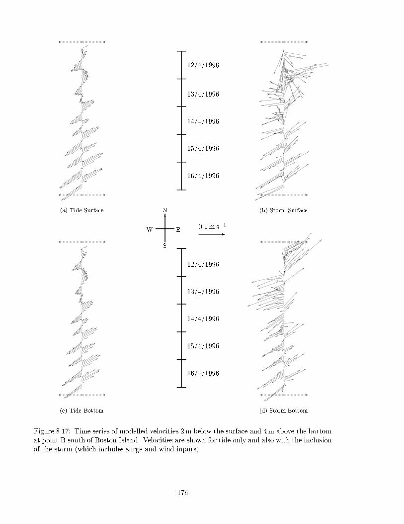
(a) Tide Surface

12/4/1996

13/4/1996

14/4/1996

15/4/1996

16/4/1996

(b) Storm Surface

0.1m s�1-

N

S

EW

66

(c) Tide Bottom

12/4/1996

13/4/1996

14/4/1996

15/4/1996

16/4/1996

(d) Storm Bottom

Figure 8.17: Time series of modelled velocities 2m below the surface and 4m above the bottomat point B south of Boston Island. Velocities are shown for tide only and also with the inclusionof the storm (which includes surge and wind inputs).

176

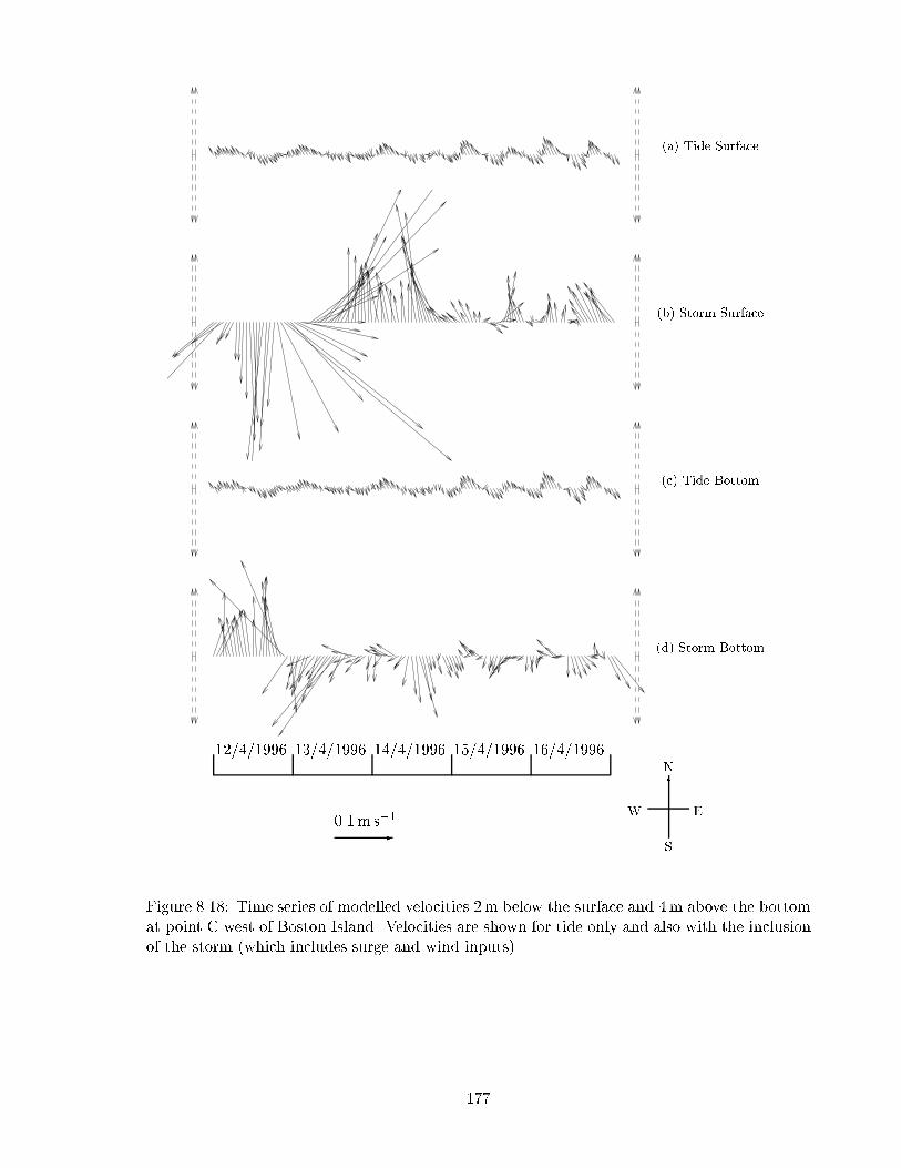
(a) Tide Surface

(b) Storm Surface

(c) Tide Bottom

(d) Storm Bottom

12/4/1996 13/4/1996 14/4/1996 15/4/1996 16/4/1996

0.1m s�1-

N

S

EW

6

Figure 8.18: Time series of modelled velocities 2m below the surface and 4m above the bottomat point C west of Boston Island. Velocities are shown for tide only and also with the inclusionof the storm (which includes surge and wind inputs).

177

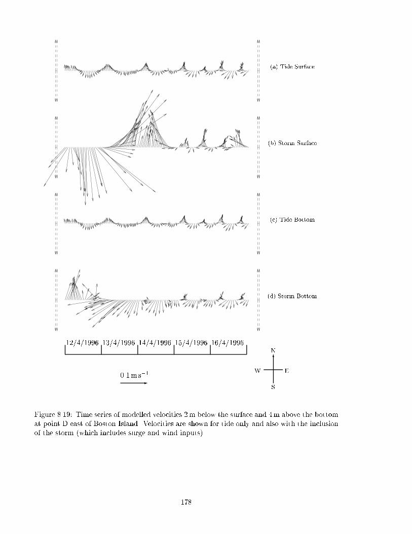
(a) Tide Surface

(b) Storm Surface

(c) Tide Bottom

(d) Storm Bottom

12/4/1996 13/4/1996 14/4/1996 15/4/1996 16/4/1996

0.1ms�1-

N

S

EW

6

Figure 8.19: Time series of modelled velocities 2m below the surface and 4m above the bottomat point D east of Boston Island. Velocities are shown for tide only and also with the inclusionof the storm (which includes surge and wind inputs).

178

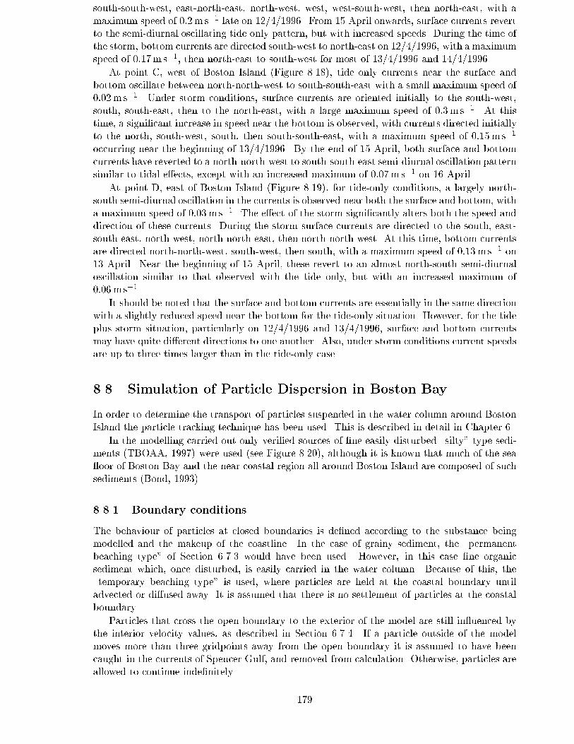
south-south-west, east-north-east, north-west, west, west-south-west, then north-east, with amaximum speed of 0:2m s�1 late on 12/4/1996. From 15 April onwards, surface currents revertto the semi-diurnal oscillating tide only pattern, but with increased speeds. During the time ofthe storm, bottom currents are directed south-west to north-east on 12/4/1996, with a maximumspeed of 0:17ms�1, then north-east to south-west for most of 13/4/1996 and 14/4/1996.

At point C, west of Boston Island (Figure 8.18), tide only currents near the surface andbottom oscillate between north-north-west to south-south-east with a small maximum speed of0:02ms�1. Under storm conditions, surface currents are oriented initially to the south-west,south, south-east, then to the north-east, with a large maximum speed of 0:3m s�1. At thistime, a signi�cant increase in speed near the bottom is observed, with currents directed initiallyto the north, south-west, south, then south-south-east, with a maximum speed of 0:15ms�1

occurring near the beginning of 13/4/1996. By the end of 15 April, both surface and bottomcurrents have reverted to a north-north-west to south-south-east semi-diurnal oscillation patternsimilar to tidal e�ects, except with an increased maximum of 0:07m s�1 on 16 April.

At point D, east of Boston Island (Figure 8.19), for tide-only conditions, a largely north-south semi-diurnal oscillation in the currents is observed near both the surface and bottom, witha maximum speed of 0:03ms�1. The e�ect of the storm signi�cantly alters both the speed anddirection of these currents. During the storm surface currents are directed to the south, east-south-east, north-west, north-north-east, then north-north-west. At this time, bottom currentsare directed north-north-west, south-west, then south, with a maximum speed of 0:13ms�1 on13 April. Near the beginning of 15 April, these revert to an almost north-south semi-diurnaloscillation similar to that observed with the tide only, but with an increased maximum of0:06ms�1.

It should be noted that the surface and bottom currents are essentially in the same directionwith a slightly reduced speed near the bottom for the tide-only situation. However, for the tideplus storm situation, particularly on 12/4/1996 and 13/4/1996, surface and bottom currentsmay have quite di�erent directions to one another. Also, under storm conditions current speedsare up to three times larger than in the tide-only case.

8.8 Simulation of Particle Dispersion in Boston Bay

In order to determine the transport of particles suspended in the water column around BostonIsland the particle tracking technique has been used. This is described in detail in Chapter 6.

In the modelling carried out only veri�ed sources of �ne easily disturbed \silty" type sedi-ments (TBOAA, 1997) were used (see Figure 8.20), although it is known that much of the sea oor of Boston Bay and the near coastal region all around Boston Island are composed of suchsediments (Bond, 1993).

8.8.1 Boundary conditions

The behaviour of particles at closed boundaries is de�ned according to the substance beingmodelled and the makeup of the coastline. In the case of grainy sediment, the \permanentbeaching type" of Section 6.7.3 would have been used. However, in this case �ne organicsediment which, once disturbed, is easily carried in the water column. Because of this, the\temporary beaching type" is used, where particles are held at the coastal boundary untiladvected or di�used away. It is assumed that there is no settlement of particles at the coastalboundary.

Particles that cross the open boundary to the exterior of the model are still in uenced bythe interior velocity values, as described in Section 6.7.4. If a particle outside of the modelmoves more than three gridpoints away from the open boundary it is assumed to have beencaught in the currents of Spencer Gulf, and removed from calculation. Otherwise, particles areallowed to continue inde�nitely.

179

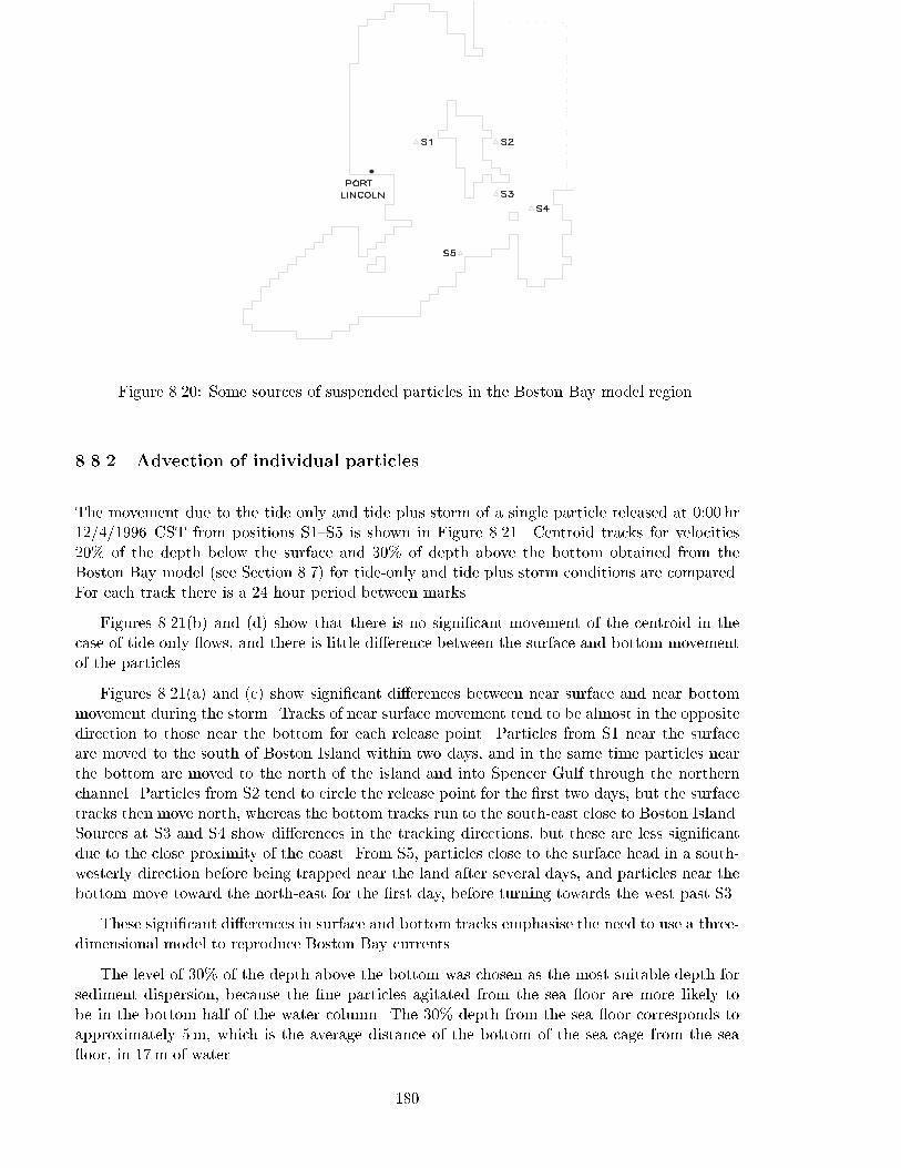
Figure 8.20: Some sources of suspended particles in the Boston Bay model region.

8.8.2 Advection of individual particles

The movement due to the tide only and tide plus storm of a single particle released at 0:00 hr12/4/1996 CST from positions S1{S5 is shown in Figure 8.21. Centroid tracks for velocities20% of the depth below the surface and 30% of depth above the bottom obtained from theBoston Bay model (see Section 8.7) for tide-only and tide plus storm conditions are compared.For each track there is a 24 hour period between marks.

Figures 8.21(b) and (d) show that there is no signi�cant movement of the centroid in thecase of tide only ows, and there is little di�erence between the surface and bottom movementof the particles.

Figures 8.21(a) and (c) show signi�cant di�erences between near surface and near bottommovement during the storm. Tracks of near surface movement tend to be almost in the oppositedirection to those near the bottom for each release point. Particles from S1 near the surfaceare moved to the south of Boston Island within two days, and in the same time particles nearthe bottom are moved to the north of the island and into Spencer Gulf through the northernchannel. Particles from S2 tend to circle the release point for the �rst two days, but the surfacetracks then move north, whereas the bottom tracks run to the south-east close to Boston Island.Sources at S3 and S4 show di�erences in the tracking directions, but these are less signi�cantdue to the close proximity of the coast. From S5, particles close to the surface head in a south-westerly direction before being trapped near the land after several days, and particles near thebottom move toward the north-east for the �rst day, before turning towards the west past S3.

These signi�cant di�erences in surface and bottom tracks emphasise the need to use a three-dimensional model to reproduce Boston Bay currents.

The level of 30% of the depth above the bottom was chosen as the most suitable depth forsediment dispersion, because the �ne particles agitated from the sea oor are more likely tobe in the bottom half of the water column. The 30% depth from the sea oor corresponds toapproximately 5m, which is the average distance of the bottom of the sea cage from the sea oor, in 17m of water.

180

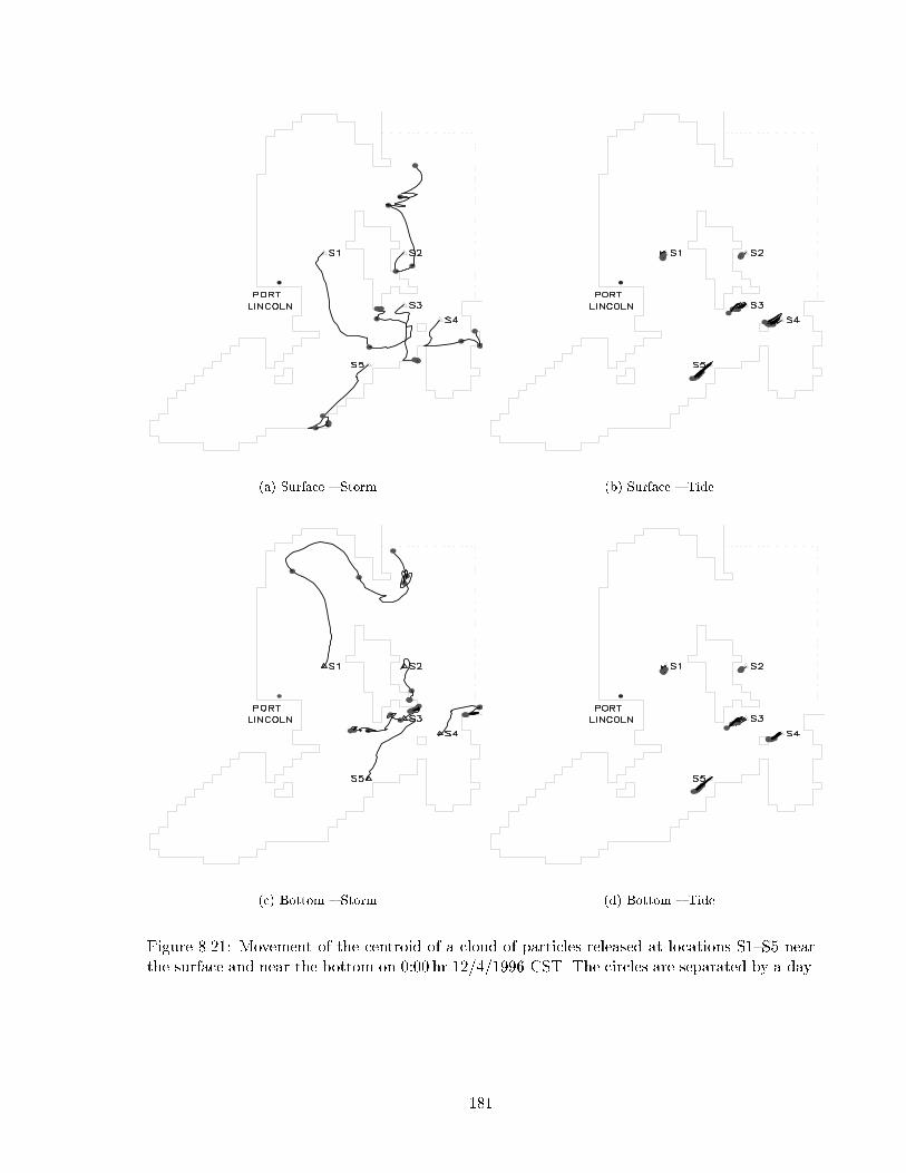
(a) Surface { Storm (b) Surface { Tide

(c) Bottom { Storm (d) Bottom { Tide

Figure 8.21: Movement of the centroid of a cloud of particles released at locations S1{S5 nearthe surface and near the bottom on 0:00 hr 12/4/1996 CST. The circles are separated by a day.

181

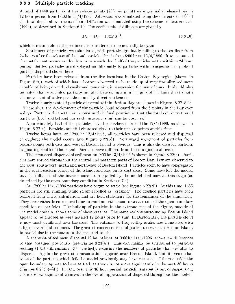
8.8.3 Multiple particle tracking

A total of 1440 particles at �ve release points (288 per point) were gradually released over a12 hour period from 18:00 hr 11/4/1996. Advection was simulated using the currents at 30% ofthe total depth above the sea oor. Di�usion was simulated using the scheme of Easton et al.(1996), as described in Section 6.10. The coe�cients of di�usion are given by

Dx = Dy = 10m2 s�1; (8.8.10)

which is reasonable as the sediment is considered to be neutrally buoyant.Settlement of particles was simulated, with particles gradually falling to the sea oor from

24 hours after the release of the �nal particle, that is from 6:00 hr on 13/4/1996. It was assumedthat settlement occurs randomly at a rate such that half of the particles settle within a 24 hourperiod. Settled particles are displayed no di�erently to particles within suspension in plots ofparticle dispersal shown here.

Particles have been released from the �ve locations in the Boston Bay region (shown inFigure 8.20), each of which has a bottom observed to be made up of very �ne silty sedimentcapable of being disturbed easily and remaining in suspension for many hours. It should alsobe noted that suspended particles are able to accumulate in the gills of the tuna due to boththe movement of water past them and by direct settlement.

Twelve hourly plots of particle dispersal within Boston Bay are shown in Figures 8.22{8.23.These show the development of the particle cloud released from the 5 points in the Bay over

4 days. Particles that settle are shown in their �nal position so that the total concentration ofparticles (both settled and currently in suspension) can be observed.

Approximately half of the particles have been released by 0:00 hr 12/4/1996, as shown inFigure 8.22(a). Particles are still clustered close to their release points at this time.

Twelve hours later, at 12:00 hr 12/4/1996, all particles have been released and dispersalthroughout the model occurs (see Figure 8.22(b)). Northward movement of particles fromrelease points both east and west of Boston Island is obvious. This is also the case for particlesoriginating south of the Island. Particles have di�used from their origins in all cases.

The simulated dispersal of sediment on 0:00 hr 13/4/1996 is shown in Figure 8.22(c). Parti-cles have spread throughout the central and northern parts of Boston Bay. Few are observed tothe west, south-west, north and north-east of Boston Island. Particles seem to have congregatedin the south-eastern corner of the Island, and also on its east coast. Some have left the model,but the in uence of the interior currents computed by the model continues at this stage (asdescribed by the open boundary condition in Section 6.7.4).

At 12:00 hr 13/4/1996 particles have begun to settle (see Figure 8.22(d)). At this time, 1366particles are still running, while 74 are labelled as \crashed". The crashed particles have beenremoved from active calculation, and are held stationary for the remainder of the simulation.They have either been removed due to random settlement, or as a result of the open boundarycondition on particles. The buildup of particles in the extreme east of the Figure, outside ofthe model domain, shows some of these crashes. The same regions surrounding Boston Islandappear to be a�ected as were noticed 12 hours prior to this. In Boston Bay, the particle cloudis now most signi�cant near the coast. The entrance to Proper Bay is also now inundated witha light covering of sediment. The greatest concentrations of particles occur near Boston Island,in particlular in the waters to the east and south.

A snapshot of sediment dispersal 12 hours later, at 0:00 hr 14/4/1996, shows few di�erencesto that obtained previously (see Figure 8.23(a)). This can mainly be attributed to particlessettling (1040 still running, 400 crashed), reducing the numbers of particles that are able todisperse. Again the greatest concentrations appear near Boston Island, but it seems thatsome of the particles which left the model previously may have returned. Others outside theopen boundary appear to have settled, as they do not move signi�cantly in the next 36 hours(Figures 8.23(b){(d)). In fact, over this 36 hour period, as sediments settle out of suspension,there are few signi�cant changes in the overall appearance of dispersal throughout the model.

182

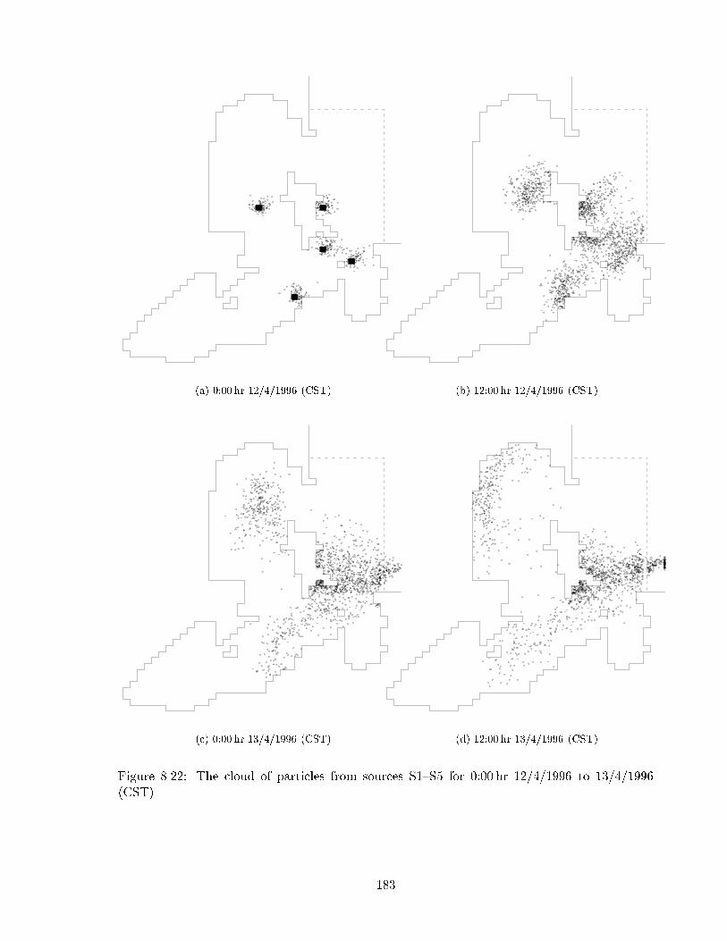
(a) 0:00 hr 12/4/1996 (CST) (b) 12:00 hr 12/4/1996 (CST)

(c) 0:00 hr 13/4/1996 (CST) (d) 12:00 hr 13/4/1996 (CST)

Figure 8.22: The cloud of particles from sources S1{S5 for 0:00 hr 12/4/1996 to 13/4/1996(CST).

183

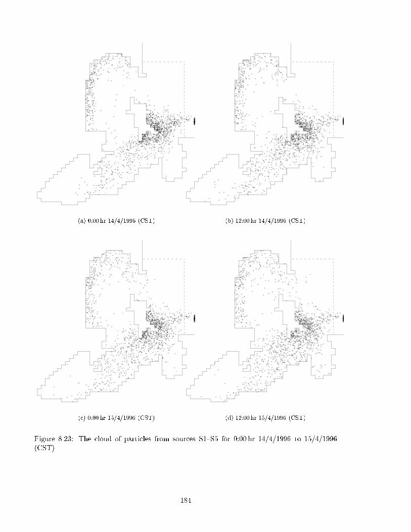
(a) 0:00 hr 14/4/1996 (CST) (b) 12:00 hr 14/4/1996 (CST)

(c) 0:00 hr 15/4/1996 (CST) (d) 12:00 hr 15/4/1996 (CST)

Figure 8.23: The cloud of particles from sources S1{S5 for 0:00 hr 14/4/1996 to 15/4/1996(CST).

184

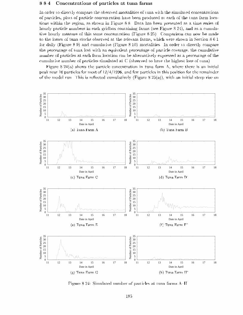
8.8.4 Concentrations of particles at tuna farms

In order to directly compare the observed mortalities of tuna with the simulated concentrationsof particles, plots of particle concentration have been produced at each of the tuna farm loca-tions within the region, as shown in Figure 8.8. Data has been presented as a time series ofhourly particle numbers in each gridbox containing farms (see Figure 8.24), and as a cumula-tive hourly measure of this same concentration (Figure 8.25). Comparison can now be madeto the losses of tuna stocks observed at the relevant farms, which were shown in Section 8.6.1for daily (Figure 8.9) and cumulative (Figure 8.10) mortalities. In order to directly comparethe percentage of tuna lost with an equivalent percentage of particle coverage, the cumulativenumber of particles at each farm location can be alternatively expressed as a percentage of thecumulative number of particles simulated at C (observed to have the highest loss of tuna).

Figure 8.24(a) shows the particle concentration in tuna farm A, where there is an initialpeak near 10 particles for most of 12/4/1996, and few particles in this position for the remainderof the model run. This is re ected cumulatively (Figure 8.25(a)), with an initial steep rise on

05

101520253035

11 12 13 14 15 16 17 18

Num

ber

of P

artic

les

Date in April

(a) Tuna Farm A

05

101520253035

11 12 13 14 15 16 17 18

Num

ber

of P

artic

les

Date in April

(b) Tuna Farm B

05

101520253035

11 12 13 14 15 16 17 18

Num

ber

of P

artic

les

Date in April

(c) Tuna Farm C

05

101520253035

11 12 13 14 15 16 17 18

Num

ber

of P

artic

les

Date in April

(d) Tuna Farm D�

05

101520253035

11 12 13 14 15 16 17 18

Num

ber

of P

artic

les

Date in April

(e) Tuna Farm E

05

101520253035

11 12 13 14 15 16 17 18

Num

ber

of P

artic

les

Date in April

(f) Tuna Farm F�

05

101520253035

11 12 13 14 15 16 17 18

Num

ber

of P

artic

les

Date in April

(g) Tuna Farm G

05

101520253035

11 12 13 14 15 16 17 18

Num

ber

of P

artic

les

Date in April

(h) Tuna Farm H�

Figure 8.24: Simulated number of particles at tuna farms A{H.

185

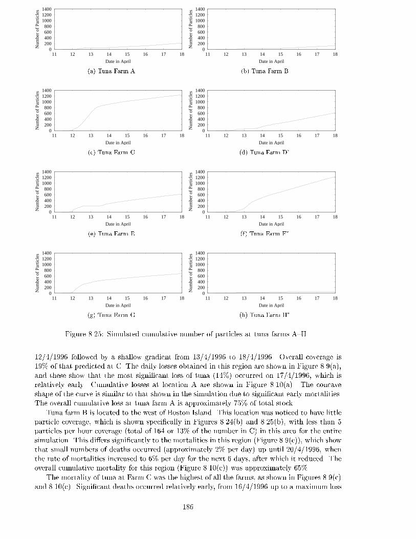
0200400600800

100012001400

11 12 13 14 15 16 17 18

Num

ber

of P

artic

les

Date in April

(a) Tuna Farm A

0200400600800

100012001400

11 12 13 14 15 16 17 18

Num

ber

of P

artic

les

Date in April

(b) Tuna Farm B

0200400600800

100012001400

11 12 13 14 15 16 17 18

Num

ber

of P

artic

les

Date in April

(c) Tuna Farm C

0200400600800

100012001400

11 12 13 14 15 16 17 18

Num

ber

of P

artic

les

Date in April

(d) Tuna Farm D�

0200400600800

100012001400

11 12 13 14 15 16 17 18

Num

ber

of P

artic

les

Date in April

(e) Tuna Farm E

0200400600800

100012001400

11 12 13 14 15 16 17 18

Num

ber

of P

artic

les

Date in April

(f) Tuna Farm F�

0200400600800

100012001400

11 12 13 14 15 16 17 18

Num

ber

of P

artic

les

Date in April

(g) Tuna Farm G

0200400600800

100012001400

11 12 13 14 15 16 17 18

Num

ber

of P

artic

les

Date in April

(h) Tuna Farm H�

Figure 8.25: Simulated cumulative number of particles at tuna farms A{H.

12/4/1996 followed by a shallow gradient from 13/4/1996 to 18/4/1996. Overall coverage is19% of that predicted at C. The daily losses obtained in this region are shown in Figure 8.9(a),and these show that the most signi�cant loss of tuna (14%) occurred on 17/4/1996, which isrelatively early. Cumulative losses at location A are shown in Figure 8.10(a). The concaveshape of the curve is similar to that shown in the simulation due to signi�cant early mortalities.The overall cumulative loss at tuna farm A is approximately 75% of total stock.

Tuna farm B is located to the west of Boston Island. This location was noticed to have littleparticle coverage, which is shown speci�cally in Figures 8.24(b) and 8.25(b), with less than 5particles per hour coverage (total of 164 or 13% of the number in C) in this area for the entiresimulation. This di�ers signi�cantly to the mortalities in this region (Figure 8.9(c)), which showthat small numbers of deaths occurred (approximately 2% per day) up until 20/4/1996, whenthe rate of mortalities increased to 6% per day for the next 6 days, after which it reduced. Theoverall cumulative mortality for this region (Figure 8.10(c)) was approximately 65%.

The mortality of tuna at Farm C was the highest of all the farms, as shown in Figures 8.9(c)and 8.10(c). Signi�cant deaths occurred relatively early, from 16/4/1996 up to a maximum loss

186

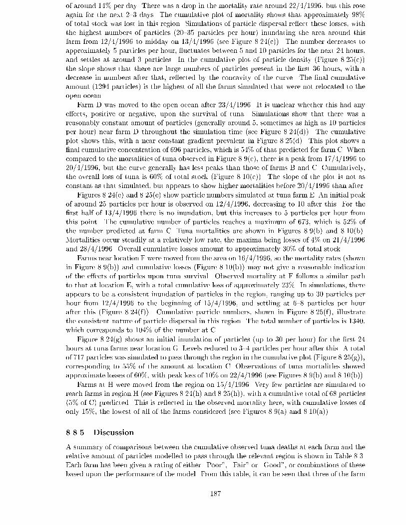
of around 14% per day. There was a drop in the mortality rate around 22/4/1996, but this roseagain for the next 2{3 days. The cumulative plot of mortality shows that approximately 98%of total stock was lost in this region. Simulations of particle dispersal re ect these losses, withthe highest numbers of particles (20{35 particles per hour) inundating the area around thisfarm from 12/4/1996 to midday on 13/4/1996 (see Figure 8.24(c)). The number decreases toapproximately 5 particles per hour, uctuates between 5 and 10 particles for the next 24 hours,and settles at around 3 particles. In the cumulative plot of particle density (Figure 8.25(c))the slope shows that there are large numbers of particles present in the �rst 36 hours, with adecrease in numbers after that, re ected by the concavity of the curve. The �nal cumulativeamount (1294 particles) is the highest of all the farms simulated that were not relocated to theopen ocean.

Farm D was moved to the open ocean after 23/4/1996. It is unclear whether this had anye�ects, positive or negative, upon the survival of tuna. Simulations show that there was areasonably constant amount of particles (generally around 5, sometimes as high as 10 particlesper hour) near farm D throughout the simulation time (see Figure 8.24(d)). The cumulativeplot shows this, with a near constant gradient prevalent in Figure 8.25(d). This plot shows a�nal cumulative concentration of 696 particles, which is 54% of that predicted for farm C. Whencompared to the mortalities of tuna observed in Figure 8.9(c), there is a peak from 17/4/1996 to20/4/1996, but the curve generally has less peaks than those of farms B and C. Cumulatively,the overall loss of tuna is 60% of total stock (Figure 8.10(c)). The slope of the plot is not asconstant as that simulated, but appears to show higher mortalities before 20/4/1996 than after.

Figures 8.24(e) and 8.25(e) show particle numbers simulated at tuna farm E. An initial peakof around 25 particles per hour is observed on 12/4/1996, decreasing to 10 after this. For the�rst half of 13/4/1996 there is no inundation, but this increases to 5 particles per hour fromthis point. The cumulative number of particles reaches a maximum of 673, which is 52% ofthe number predicted at farm C. Tuna mortalities are shown in Figures 8.9(b) and 8.10(b).Mortalities occur steadily at a relatively low rate, the maxima being losses of 4% on 21/4/1996and 28/4/1996. Overall cumulative losses amount to approximately 30% of total stock.

Farms near location F were moved from the area on 16/4/1996, so the mortality rates (shownin Figure 8.9(b)) and cumulative losses (Figure 8.10(b)) may not give a reasonable indicationof the e�ects of particles upon tuna survival. Observed mortality at F follows a similar pathto that at location E, with a total cumulative loss of approximately 23%. In simulations, thereappears to be a consistent inundation of particles in the region, ranging up to 30 particles perhour from 12/4/1996 to the beginning of 15/4/1996, and settling at 6{8 particles per hourafter this (Figure 8.24(f)). Cumulative particle numbers, shown in Figure 8.25(f), illustratethe consistent nature of particle dispersal in this region. The total number of particles is 1340,which corresponds to 104% of the number at C.

Figure 8.24(g) shows an initial inundation of particles (up to 30 per hour) for the �rst 24hours at tuna farms near location G. Levels reduced to 3{4 particles per hour after this. A totalof 717 particles was simulated to pass through the region in the cumulative plot (Figure 8.25(g)),corresponding to 55% of the amount at location C. Observations of tuna mortalities showedapproximate losses of 60%, with peak loss of 10% on 22/4/1996 (see Figures 8.9(b) and 8.10(b)).

Farms at H were moved from the region on 15/4/1996. Very few particles are simulated toreach farms in region H (see Figures 8.24(h) and 8.25(h)), with a cumulative total of 68 particles(5% of C) predicted. This is re ected in the observed mortality here, with cumulative losses ofonly 15%, the lowest of all of the farms considered (see Figures 8.9(a) and 8.10(a)).

8.8.5 Discussion

A summary of comparisons between the cumulative observed tuna deaths at each farm and therelative amount of particles modelled to pass through the relevant region is shown in Table 8.3.Each farm has been given a rating of either \Poor", \Fair" or \Good", or combinations of thesebased upon the performance of the model. From this table, it can be seen that three of the farm

187

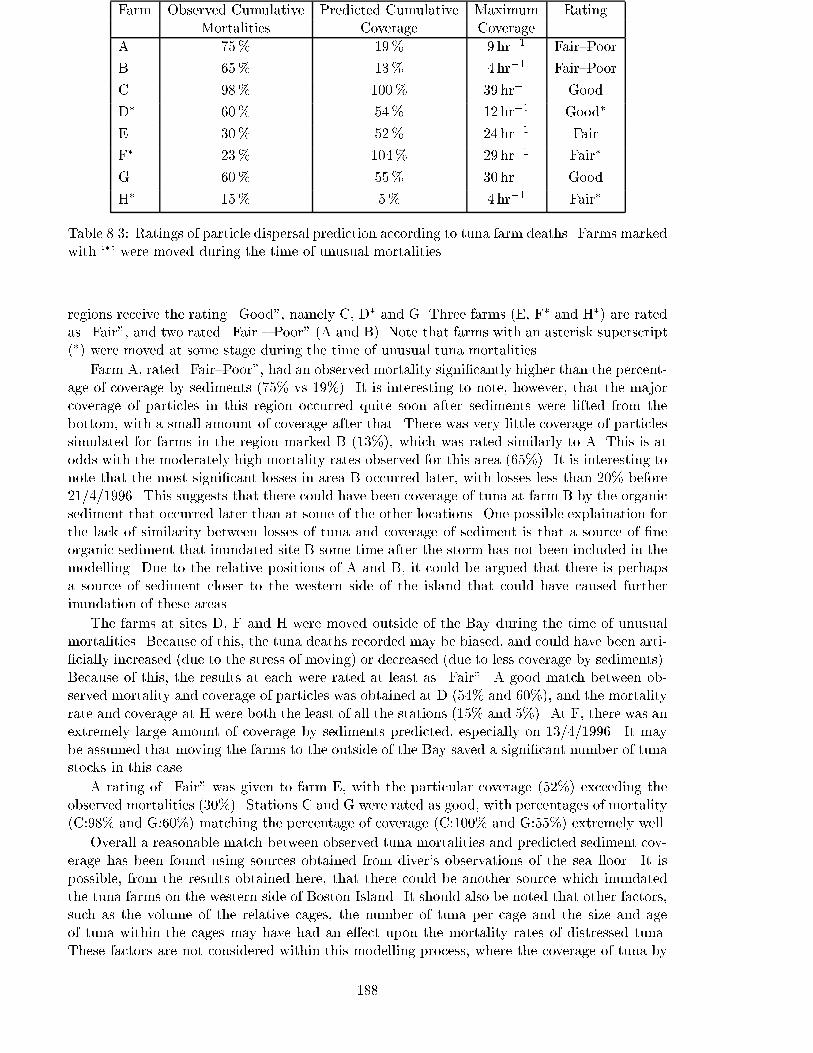
Farm Observed Cumulative Predicted Cumulative Maximum RatingMortalities Coverage Coverage

A 75% 19% 9hr�1 Fair{Poor

B 65% 13% 4hr�1 Fair{Poor

C 98% 100% 39 hr�1 Good

D� 60% 54% 12 hr�1 Good�

E 30% 52% 24 hr�1 Fair

F� 23% 104% 29 hr�1 Fair�

G 60% 55% 30 hr�1 Good

H� 15% 5% 4hr�1 Fair�

Table 8.3: Ratings of particle dispersal prediction according to tuna farm deaths. Farms markedwith `�' were moved during the time of unusual mortalities.

regions receive the rating \Good", namely C, D� and G. Three farms (E, F� and H�) are ratedas \Fair", and two rated \Fair { Poor" (A and B). Note that farms with an asterisk superscript(�) were moved at some stage during the time of unusual tuna mortalities.

Farm A, rated \Fair{Poor", had an observed mortality signi�cantly higher than the percent-age of coverage by sediments (75% vs 19%). It is interesting to note, however, that the majorcoverage of particles in this region occurred quite soon after sediments were lifted from thebottom, with a small amount of coverage after that. There was very little coverage of particlessimulated for farms in the region marked B (13%), which was rated similarly to A. This is atodds with the moderately high mortality rates observed for this area (65%). It is interesting tonote that the most signi�cant losses in area B occurred later, with losses less than 20% before21/4/1996. This suggests that there could have been coverage of tuna at farm B by the organicsediment that occurred later than at some of the other locations. One possible explaination forthe lack of similarity between losses of tuna and coverage of sediment is that a source of �neorganic sediment that inundated site B some time after the storm has not been included in themodelling. Due to the relative positions of A and B, it could be argued that there is perhapsa source of sediment closer to the western side of the island that could have caused furtherinundation of these areas.

The farms at sites D, F and H were moved outside of the Bay during the time of unusualmortalities. Because of this, the tuna deaths recorded may be biased, and could have been arti-�cially increased (due to the stress of moving) or decreased (due to less coverage by sediments).Because of this, the results at each were rated at least as \Fair". A good match between ob-served mortality and coverage of particles was obtained at D (54% and 60%), and the mortalityrate and coverage at H were both the least of all the stations (15% and 5%). At F, there was anextremely large amount of coverage by sediments predicted, especially on 13/4/1996. It maybe assumed that moving the farms to the outside of the Bay saved a signi�cant number of tunastocks in this case.

A rating of \Fair" was given to farm E, with the particular coverage (52%) exceeding theobserved mortalities (30%). Stations C and G were rated as good, with percentages of mortality(C:98% and G:60%) matching the percentage of coverage (C:100% and G:55%) extremely well.

Overall a reasonable match between observed tuna mortalities and predicted sediment cov-erage has been found using sources obtained from diver's observations of the sea oor. It ispossible, from the results obtained here, that there could be another source which inundatedthe tuna farms on the western side of Boston Island. It should also be noted that other factors,such as the volume of the relative cages, the number of tuna per cage and the size and ageof tuna within the cages may have had an e�ect upon the mortality rates of distressed tuna.These factors are not considered within this modelling process, where the coverage of tuna by

188

organic sediment is assumed to be the major factor in mortality.

8.9 Summary

A three-dimensional tide and storm surge prediction model of the Boston Bay region, SouthAustralia, has been constructed. This has been tested for the prediction of sea level and currentvelocity for a test case, and has then been applied to hindcasting the in uence of the April 1996storm on the Bay. It was found that external surges had a signi�cant e�ect upon currents,particularly to the north and south of Boston Island. Wind �elds caused a signi�cant increasein current velocities, with surface and bottom current directions often in opposition.

A comparison of tracks of single particles conducted for depths near the surface and sea oor found that particles often moved in opposite directions, with those released from somepoints found to move to opposite ends of the Bay after �ve days.

The particle tracking routine has been applied, using near bottom predictions of velocity, tosimulate the dispersal of �ne organic sediments which were stirred from the sea oor by storm-induced wind waves. The spread of particles was then compared to mortalities of tuna cagedin farms within the region during this time. In general a good match was obtained between thecumulative tuna losses and the concentrations of particles predicted.

189

190