Extractive States:The Case of the Italian Unification.∗

Guilherme de Oliveira and Carmine GuerrieroColumbia Law School and University of Bologna

March 31, 2017

Abstract

Despite the huge evidence on the adverse impact of extractive policies, we still lack aframework that identifies their determinants. Here, we lay out a two-region, two-socialclass model for thinking about this issue, and we exploit its implications to identifythe causes of the opening of the present-day divide between North and South of Italy.Differently from the extant literature, we document that it arose because of the region-specific policies selected between 1861 and 1911 by the elite of the Kingdom of Sardinia,which annexed the rest of Italy in 1861. While indeed pre-unitary land property taxrevenues and railway diffusion were shaped by each region’s farming productivity butnot by its political relevance for the Piedmontese elite, the opposite was true for thepost-unitary ones. Moreover, post-unitary tax distortions and the severity of the re-maining extractive policies—captured by the region’s taxation capacity and politicalrelevance—determined the North-South gaps in culture, literacy, and development butnot that in the manufacturing industry value added. Consequently, extraction neithereased the formation of an unitary market nor favored industrialization. Our resultsremain robust to considering fixed region and time effects and the structural conditionsdifferentiating the two blocks in 1861, i.e., pre-unitary inclusiveness of political insti-tutions, land ownership fragmentation, and inputs. Crucially, our framework clarifiesthe incentives of dominating groups in other unions, e.g., post-Civil War USA and EU.Keywords: Extractive States; Political Union; Culture; State Capacity.JEL classification: H20; H70; N4; Z10.

∗We are indebted to Brian A’Hearn, Toke Aidt, Marco Casari, Decio Coviello, Giuseppe Dari-Mattiacci,Andy Hanssen, Eliana La Ferrara, Raffaella Paduano, Enrico Perotti, Torsten Persson, Laura Rondi, Avra-ham Tabbach, Guido Tabellini, Davide Ticchi, Paola Valbonesi, and seminar participants at Bologna, IMT,Maastricht University, UvA, and at the 2014 Winter Meeting of the Econometric Society for the insightfulcomments, to Carlo Ciccarelli, Mark Dincecco, Giovanni Federico, Stefano Fenoltea, Luigi Guiso, GiovanniIuzzolino, Paolo Malanima, Luca Pennacchio, Guido Pescosolido, Paolo Pinotti, Giovanni Vecchi, and An-drea Vindigni for the data provided, and to the staffs of the Biblioteca Nazionale Centrale and the BibliotecaSVIMEZ, both in Roma, for the guidance. Guilherme de Oliveira wishes to thank the “Fundacao para aCiencia e Tecnologia” for support through the Grant SFRH/BD/76122/2011, whereas Carmine Guerrierowishes to thank EIEF for hosting him while the first version of this paper was written. Corresponding author:Carmine Guerriero. Address: Strada Maggiore 45, 40125 Bologna, Italy. E-mail: c.guerriero@unibo.it

“The vast majority of the population [. . .] feels entirely cut off from our institutions. People see them-selves subjected to the State and forced to serve it with their blood and their money, but they do not feelthat they are [an] organic part of it.” (Sydney Sonnino, Speech to the Chamber of Deputies, 30 March 1881).

1 Introduction

Despite the huge evidence documenting that extractive institutions and policies can limit

the access to rents discouraging in turn innovation (North et al., 2009) and can undermine

both property rights protection and contract enforcement (Acemoglu and Robinson, 2012),

we still lack a framework that identifies their determinants. Here, we lay out a two-region,

two-social class model for thinking about this issue, and we exploit its implications to propose

a novel account of the present-day economic divide between North and South of Italy.1

A well-known literature has traced back this gap to the diverse political trajectories

followed by the two clusters during the Middle Ages (Putnam et al., 1993). In particular, the

experience of more inclusive political institutions—i.e., the communes—would have helped

Northern Italy develop a stronger culture of cooperation easing economic interactions (Guiso

et al., 2016; Tabellini, 2010). Recent contributions however have raised several doubts on this

slant. First, Boranbay and Guerriero (2016) show for Europe that instead the main driver of

present-day culture has been the medieval need of sharing climate-driven consumption risk

and that, up to the 17th century, the two clusters displayed similar cultural endowments.

Second, a growing body of research reveals that the two groups were similarly underdeveloped

in 1861 (Federico, 2007; Ciccarelli and Fenoaltea, 2013). Inspired by this evidence, we

document that the opening of the present-day divide is the result of the region-specific

policies selected between 1861 and 1911 by the elite of the Kingdom of Sardinia, which

annexed the rest of Italy in 1861. They penalized more the regions farther away from the

fiercer enemy of the House of Savoy and so less politically relevant for the Piedmontese elite.

In the model, we consider two regions, which are first independent and then unified by

a completely unforeseen shock similar to the one that originated the unitary state. The

Northern region represents the Kingdom of Sardinia, whereas the Southern one stands for

1To elaborate, in 2008 Southern Italy displayed a nine percent lower share of respondents to the EuropeanValue Study reporting “tolerance and respect for other people” as important qualities children should beencouraged to learn and a 40 percent lower income per capita than Northern Italy (Iuzzolino et al., 2011).

2

any of the other states annexed by the Kingdom of Italy in 1861. Each region is inhabited by

a mass zero elite and a mass one citizenry, who consumes the untaxed supply of a private good

and a region-specific public good whose production is financed through the tax revenues not

appropriated by the elite. The private good technology is multiplicative in the region-specific

productivity and the citizenry’s investment in an input that can be seen as either a culture of

cooperation or human capital. The first interpretation links directly our setup to the extant

literature on the medieval determinants of the present-day divide. Under autarky, each elite

selects her region’s tax rate by maximizing the sum of the citizenry’s welfare and the rents

net of linear tax-collection costs. Thus, equilibrium tax revenues fall with the marginal tax-

collection costs and, because these are sizable, with the taxable value and thus the regional

productivity. Under political union instead, both region-specific tax rates are selected by the

Northern elite, who is less concerned with the Southern citizenry’s welfare and appropriates

from the South relatively more than the Southern elite can under autarky. In particular, the

extractive power of the Northern elite is sufficiently strong to make taxation of the South

profitable at the margin. These assumptions are consistent with the fact that the unitary

state exercised a tight control on the annexed regions and was dominated by the elite of the

Kingdom of Sardinia, who was chiefly interested in the Northern export-oriented farming

and industry. The mix between stronger extractive capacity and her limited concerns with

the South leads the Northern elite to raise from this region tax revenues rising with the

South’s productivity and falling with both the marginal tax-collection costs and the South’s

political relevance, i.e., the weight the Northern elite attaches to the Southern citizenry’s

welfare. In addition, extraction from the South is larger than under autarky, provided that

the South’s technology is not too backward, and pushes the Southern citizenry to prefer

private to public good production. Hence, the Southern citizenry’s investment and welfare

rise with the factors limiting taxation, like the marginal tax-collection costs and the political

relevance, and unification damages the South when it is not sufficiently salient for the North.

To test these predictions, we analyze the thirteen present-day Italian regions annexed

by the Kingdom of Italy between 1861 and 1911 but not part of the Kingdom of Sardinia.

Being the Italian economy mainly agrarian over our 1801-1911 sample, we proxy the extent

of extraction first and foremost with the land property taxation. Given the available in-

3

formation however, we do not study land property tax rates but the relative revenues per

capita. Land property tax rates have been region-specific over the whole sample and, absent

developed financial markets, dramatically shaped the landowners’ capacity to invest in new

farming technologies and the industry. Turning to the regional productivity, we rely upon

the geographic drivers of the profitability of the main export-oriented farming sectors, i.e.,

arboriculture and sericulture. Next, we use as inverse metrics of the marginal tax-collection

costs a measure of state capacity, i.e., the share of previous decade in which the state to

which the region belonged partook in external wars. Finally, we propose as an inverse proxy

for political relevance the distance between each region’s main city and the capital of the

fiercer enemy of the House of Savoy. Being our model applicable to any extent of extraction,

these two proxies also capture the impact on the South of the other distortionary policies

selected by the post-unitary government and illustrated in our historical analysis.

Consistent with our model, while the pre-unitary revenues from land property taxes in

1861 lire per capita were shaped by each region’s farming productivity but not by its political

relevance for the Piedmontese elite, the opposite was true for the post-unitary ones. More-

over, post-unitary tax distortions—proxied with the difference between the observed revenues

and the counterfactual ones forecasted through pre-unitary estimates—and the severity of

the remaining extractive policies—captured by the region’s taxation capacity and political

relevance—determined the North-South gaps in culture, literacy, and development. Since

our proxies for the drivers of extraction are driven by either geographic features indepen-

dent of human effort or events outside the control of the policy-makers, reverse causation is

not an issue. Nevertheless, our results could still be produced by unobserved heterogeneity.

To evaluate this aspect, we follow a two-step strategy. First, we control not only for fixed

region effects, but also for time effects and their interaction with the structural conditions

differentiating the two blocks in 1861, i.e., pre-unitary inclusiveness of political institutions,

land ownership fragmentation, coal price, and the railway length. Including these controls

has little effect on our estimates. Second, we build on Oster (2016), and we calculate that on

average selection on unobservables would have to be about 4 times greater than selection on

observables to completely explain away our results. Given the very high fit of our regressions,

this is unlikely. Finally, two extra results rule out the possibility that extractive policies were

4

the acceptable price for the Italian development (Romeo, 1987). First, extraction did not

shape the manufacturing sector value added and in turn industrialization. Second, while

the pre-unitary length of railway additions in km per square km was only affected by the

region’s farming productivity, the post-unitary diffusion of the rail system was only driven

by the regional political relevance resulting useless in the formation of an unitary market.

Albeit a long literature has related the present-day divide to post-unitary policies (Sereni,

1947; Salvemini 1963; Romeo, 1987; Cafagna, 1989), nobody has provided a framework

clarifying how these policies solved the unitary government’s trade-off between extraction-

related losses—i.e., investment distortions, tax-collection costs, and military weakness—and

rent-seeking gains.2 In doing this, we also contribute to the aforementioned literature on

extractive institutions by endogenizing the extent of extraction in a setup sufficiently general

to be applied to other instances. Recent examples are the German opposition to the post-

2011 rescue packages demanded by Greece (Guiso et al., 2015) and the tensions between

the Basque Country (Northern Ireland) and the Spanish (UK) government (Abadie and

Gardeazabal, 2003; Besley and Mueller, 2012), whereas a case in point contemporaneous to

the natural experiment we focus on is the post-Civil War gap between the ex-Confederate

states and the territories that sustained the Union during the war. To confirm the external

validity of our analysis, we study this last instance, and we provide evidence that the growing

divide between the two clusters was related to the tax burdens imposed on them by the federal

government, which was initially dominated by the ex-Union states.

The paper proceeds as follows. In section 2, we review some key facts about 19th century

Italy to motivate our model, which we illustrate in section 3. In section 4 then, we state the

model empirical implications, which we test in section 5. Finally, we present our conclusions

in section 6, and we gather both tables and figures in the appendix.

2 Italy Before and After the Unification: A Primer

Next, we describe the political and economic contexts of the Italian regions over the

1801-1911 period, detailing at the same time the evolution of public policies.

2By studying the determinants of regional tax policies and public spending, we also contribute to the literatureon public goods, internal and external conflicts, and the size of nations (Alesina and Spolaore, 2005).

5

2.1 The Era of Risorgimento

The Congress of Vienna divided Italy in eight absolutists states: the Kingdom of Sardinia,

formed by Liguria, Piedmont, and Sardinia and ruled by the Piedmontese House of Savoy;

the Kingdom of Lombardy-Venetia under the direct control of Austria; the Grand Duchy of

Tuscany and the Duchies of Modena and Parma, all in the hands of branches of the Habsburg

dynasty; the Duchy of Lucca then absorbed by Tuscany in 1847; the Papal State; and, to

the south of Lazio and Marche, the Kingdom of the Two Sicilies ruled by the Bourbons.3

This division re-established the status quo preceding the Napoleonic conquests and served

two key purposes. First, it deprived the Bourbons of any interest in waging war being their

only neighbor the Pope, who in turn was constrained by his religious role. Second, it kept in

check Austria and France by establishing the Kingdom of Sardinia as a buffer state between

the two powers. Exactly this balance fed the ambitions of the House of Savoy who became

the champion of the Italian liberals. Supported by urban workers and lower military ranks,

the liberals longed to establish a unitary state by organizing a series of subversive acts in

the wake of the unrests of 1820, 1830, and 1848. Even if none of these turmoils overthrew a

pre-unitary regime, they forced the absolutist rulers to implement some of the liberal laws

brought about by the Napoleonic armies and inspired by the French revolution.

The liberal wave flooded the whole peninsula but was particularly effective in washing

away several long-lived feudal privileges from the Kingdom of the Two Sicilies, where one

third of the clerical and common lands were privatized and the feudal system was finally abol-

ished in 1806 [Pescosolido 2014, p. 50-58]. Such an institutional discontinuity did not release

the Italian peasants from their destitution but allowed a rising class of bourgeoisie, attracted

by the mid of the 19th century rise in the international demand, to acquire part of the nester

nobility’s domains and prioritize export-oriented over subsistence farming [Pescosolido 2014,

p. 29-30 and 39-40]. In particular, arboriculture and sericulture soon gained a net domi-

nance accounting by 1859 for respectively the 33 and 14 percent of total export, while next

two—in terms of export relevance—cultivations—i.e., wine and hemp—racked up the seven

percent of total export (Ministero dell’Agricoltura, Industria e Commercio, 1864). Albeit

more lucrative than wheat breeding—sixty times in the arboriculture case [Dimico et al.

3Our historical account is based on Killinger (2002), Duggan (2008), Paoletti (2008), and Riall (2009).

6

2012, p. 7], both activities were also more capital intensive. Silk indeed is obtained from

the fibers of the cocoons of the mulberry silkworm larvae dissolved in boiling water and

then spun through reels powered at the time by watermills. This need of water favored the

concentration of sericulture in the irrigated Po valley [Federico 2009, p. 18]. Over and above

irrigation ditches, citrus and olive trees require a temperature above 4 Celsius degrees: this

last feature explains their almost exclusive diffusion in the South [Dimico et al. 2012, p. 8].

Farming productivity increased in both the sharecropping-based Northern farms and the

Southern latifundia, which maintained a primacy over the 19th century (Federico, 2007).4

Table 2 summarizes these patterns by using our proxies for farming productivity and differ-

entiating the thirteen regions analyzed in our empirical exercise according to their political

relevance for the Piedmontese elite as inversely measured by Distance-to-Enemies, which is

the distance between each region’s main city and the capital of the fiercer enemy of the House

of Savoy (see section 4 for more details and table 1 for sources and construction). To illus-

trate, Veneto displays the lowest average value of Distance-to-Enemies being the only region

bordering either Austria or France, and so we treat it as the “high” political relevance cluster.

Similarly, we label the other regions with below-average values of Distance-to-Enemies—i.e.,

Abruzzi, Emilia Romagna, Lombardy, Marche, Tuscany, and Umbria—the “middle” political

relevance group and the remainder—i.e., Apulia, Basilicata, Calabria, Campania, Lazio, and

Sicily—the “low” political relevance group. We also refer to the latter as “South” and to the

union of the high and middle political relevance groups with both Liguria and Piedmont,

which represented the leading regions of the Kingdom of Sardinia, as “North.” As table 2

reveals, the South was moderately inferior than the middle and high political relevance clus-

ter in the sericulture and wheat breeding sectors but greatly (moderately) superior in the

arboriculture one (in terms of gross saleable farming product per employee, i.e., GSP-L).

After two centuries of decline (Malanima, 2010), the Italian population doubled over the

1800-1860 period but the peninsular economy remained essentially agrarian and so the GDP

per capita stagnated until the 1880s against a background of regional differences (see upper-

left graph in figure 1).5 To illustrate, the South displayed for all the pre-unitary period

4The latter supported larger investments by assuring the peasants credit and job security (Petrusewicz, 1996).5To illustrate, in 1861 the 69 percent of the active population was employed in the agricultural sectors(SVIMEZ, 2011), and only the one percent worked exclusively in the industry [Pescosolido 2014, p. 130].

7

an income level significantly higher than the North but this advantage,6 which was mainly

driven by the idiosyncratic shocks to the regional export-oriented sectors,7 did not help it

fill the enormous gap with the leading European countries on the road to industrialization

[Pescosolido 2014, p. 77-84]. Just to name a few examples, in 1861 the number of spindles in

respectively the North and South corresponded to the 0.8 and 0.2 percent of the English one,

whereas the 1861 iron production amounted to the even lower levels of 0.46 and 0.04 percent

of the UK one (Pescosolido, 2011). The causes of this common backwardness—similarly

revealed by the 1861 values added of the textile and manufacturing sectors (see table 2)—

were multiple and ranged from the scarcity of coal and navigable rivers to the mix of the

underdevelopment of railway, roads, and merchant navy and the shortage of both human and

real capital [Pescosolido 2014, p. 89-101]. None of these initial structural conditions displayed

however significantly different values in the low and middle-high political relevance clusters,

save for the limited gaps in railway length and coal price (see table 2).8 In this respect, only

the Kingdom of Sardinia seemed ready to take on the Second industrial revolution challenge

with its significantly larger endowment of human capital and more efficient textile sector

both gained through a more vigorous public investment effort [Zamagni 1980, p. 124-126].9

The 1848 defeat in the Austro-Sardinian War indeed forced Carlo Alberto to abdicate

in favor of his son Vittorio Emanuele II, who upheld a liberal constitution to calm down

the internal uprisings and gain support for his territorial ambitions. This change allowed

the rising liberal class to obtain a larger public spending in railway and other valued public

goods, like literacy, in exchange for the acceptance of larger military expenses. None of the

other Italian states could obtain a similar balance [Duggan 2008, p. 261]. On the one hand,

Vienna avoided unrests and any grant of rights in the Lombardy-Veneto by appeasing local

6We express this and the other monetary variables in 1861 lire per capita employing the Malanima’s (2006)and Baffigi’s (2011) price indexes. While the underlying 1871-1911 data are collected from Vecchi (2011), the1801-1861 figures are constructed combining the series for the Northern regions reported in Malanima (2006),those for the whole country proposed by Malanima (2010), and population data from SVIMEZ (2011).

7The Southern arboriculture sector was hit by the 1825-1834 fall in international prices, while the Northernsilk production was halved by the 1840-1860 Pebrine epidemic [Pescosolido 2014, p. 39-41 and 145].

8The financial sector exhibited however the following variation. While the Northern markets were populatedby both small institutes—i.e., “casse di risparmio”—and medium-sized commercial banks, the Southernmarkets were still dominated by a plethora of medieval micro-credit institutions [Pescosolido 2014, p. 90-91].

9To illustrate, in 1861 Piedmont and Liguria displayed on average 55.25 percentage points of illiterates and a0.007 textile industry value added in thousands of 1861 lire per capita (see for sources table 1).

8

elites through high nonmilitary expenditures and artificially low tax rates [Dincecco et al.

2011, p. 900]. On the other hand instead, the Bourbons—scared by the 1820 and 1848

domestic unrests—escaped democratic reforms by rising the military spending and, because

of the population’s aversion to taxation, by squeezing nonmilitary expenditures [Pescosolido

2014, p. 96]. A similar aversion to novel duties, together with less ferocious internal conflicts,

kept taxation and spending low in the remaining states [Dincecco et al. 2011, p. 898-899].

Figure 1 depicts these patterns. While the bottom-left graph reports, in default of in-

formation on the tax rates, the revenues from land property taxes in 1861 lire per capita,

the bottom-right one displays the decennial change in the railway network in km per square

km. Land property taxes, which represented the largest direct tax and hit the land prof-

itability estimated by one of the nine existing regional cadastres,10 remained up to the 1850s

larger in the South, whereas investments in railway diffusion, which represented the largest

nonmilitary expenditure, were trifle before 1840 and barely higher in the North at unification.

2.2 Italian Unification and the Rise of the North-South Divide

Over the 1850s, the power of the Kingdom of Sardinia’s parliament relative to the king

grew steadily and its leader became count Camillo of Cavour, who was appointed prime

minister in 1852. Cavour realized that the Savoys could not fight Austria alone and, thus,

sustained France in the Crimean War (1853-1856) to win the favor of Napoleon III. This

attempt was such a success that the Kingdom of Sardinia and France first signed a secret

pact against Austria and then defeated its military in Lombardy in 1859. This victory

triggered insurrections in Tuscany, Giuseppe Garibaldi’s conquest of the South, and the

invasion of the Papal State. The Kingdom of Italy was proclaimed on March 17th 1861.

“A narrow elite of northerners dominated [the new government and] bureaucracy. Not

until 1887 did a southerner become prime minister [i.e., Crispi]. The king preferred if he

could to have a premier from Piedmont (with whom he could speak in dialect)” [Duggan

2014, p. 141] and, indeed, Piedmontese was the 58 percent of all the 1861-1911 prime

ministers, share which rises to the 85 percent when the entire North is considered (see

also upper-right graph in figure 1) and is similar to what one would obtain by focusing on

10This measure was obtained through either geometrical or descriptive data (Parravicini, 1958).

9

lower-ranked policy-makers.11 “In the 1890s [indeed] 60 per cent of the top administrative

posts were occupied by Lombards, Venetians, or Piedmontese” [Duggan 2014, p. 141] and

the provinces were run by government-appointed prefects, each of whom “was a personal

friend of the king or the prime-minister and [. . . ] usually came from Piedmont. [Moreover,

the commune’s] mayor was nominated by the central government [and the prefect could]

oversee, and if need be, veto, municipal decisions” [Duggan 2014, p. 139]. Empowered by

its new European stand and military power [Pescosolido 2014, p. 96], this Piedmontese-led

ruling class favored the Northern export-oriented farming and manufacturing industry while

selecting trade, financial, and public spending policies and the Northern population when

levying the taxes necessary to finance public spending [Sereni, 1947; Salvemini 1963, p. 286;

Romeo, 1987; Cafagna, 1989]. Since the underdevelopment of the banking sector and the

Malthusian nature of the agrarian economy made the participation in the second Industrial

revolution dependent on the after tax farming profits only, these policies dramatically shaped

the relative performance of the two clusters [Pescosolido 2014, p. 90-92, 118-120, and 157].

To begin with, the 1861 introduction of the Piedmontese custom tariffs decreased by

80 percent the average Southern duties (Pescosolido, 2011). This liberal reform initially

fostered the very lucrative exports of olive oil, citrus, and silk but then irremediably exposed

these activities to the fall in the farm crops prices determined in the 1880s by the mix of

the soaring international supply and the advances in maritime transportation [Iuzzolino et

al. 2011, p. 20]. Between 1887 and 1891, the exports of citrus fruits, oil, and wine roughly

halved, whereas those of silk remained stable [Pescosolido 2014, p. 198-201 and 224-228].

This juncture allowed the Po Valley nester nobility and the industrial triangle entrepreneurs

to form a new ruling coalition and so direct in 1887 a protectionist reform uniquely aimed at

protecting wheat breeding and those Northern manufacturing industries that had artificially

survived the liberal years thanks to the newborn state intervention [Pescosolido 2014, p. 64,

177-182, and 202; Ministero dell’Agricoltura, Industria e Commercio 1890, p. 419-420]. To

illustrate, while the Northern textile industry fully dominated the national allocation of the

military clothing contracts, the monopoly of both the steamboat construction and the Italian

navigation was assigned to Genoese firms with the consequent exclusion of the Neapolitan

11The share of ex-Kingdom of Sardinia(North)-born ministers was 35 (64) percent (Corbetta and Piretti, 2008).

10

ones, which albeit more developed at unification went bankrupt in the 1870s [Pescosolido

2014, p. 182-184 and 203]. A similar logic guided the organization of land reclamation

with only four per cent of the relative spending invested in the South before World War I

[Iuzzolino et al. 2011, p. 23], the allocation of coal mining permits and public contracts to

the newborn iron and steel industry,12 the exclusive assignment to the Piedmontese Banca

Nazionale of the faculty of opening new branches and issuing banknotes convertible in the

entire country [Pescosolido 2014, p. 151], and above all the public investment in railway,

which constituted the 67 (53) percent of the 1861-1881(1911) Italian public spending (Picci,

2002). To elaborate, Liguria and Piedmont enjoyed over the 1861-1881(1911) period an

average railway spending of 874 (457)—1861—lire per square km, which was 12 (3) times

bigger than that received by Veneto and 18 (4) times higher than that gained by the other

regions. Moreover, the 1885 reform handed the vast majority of the property of the railway

industry to Northern hands [Pescosolido 2014, p. 159-167]. Crucially, the real purpose of

this effort “was more the military one of controlling the national territory, especially in the

South, than favoring commerce [. . . The] railway fares acted in many cases as customs duties,

making it more economic for the South to export goods abroad by sea rather than try to

sell its products to the North via railway” [Iuzzolino et al. 2011, p. 22].

Crucially, such an impressive infrastructural program was financed through highly unbal-

anced rises in the land property tax, which as discussed above was the most important shifter

of investment (Parravicini, 1958). After an initial phase in which a 10 percent surcharge was

added to the pre-unitary tax rates, the 1864 reform fixed a target revenue to be raised—i.e.,

“contingente”—equal to the 1863 yield plus 20 millions—i.e., 125 millions—allocating it to

nine fiscal districts resembling the pre-unitary states (law 1831/1864).13 The ex-Papal State

took on the 10 percent of the contingente, the ex-Kingdom of Two Sicilies the 40 percent, and

the rest of the Kingdom of Italy (ex-Kingdom of Sardinia) only 29 (21) percent. To further

weigh this burden down, between 1867 and 1868, two other 10 percent surcharges were added

to the contingente creating the disparities between high and middle-low political relevance

12While the permits to mine for coal in Elba were assigned to the Northern Terni-Banca Commerciale group,the only Southern blast furnace was opened in Bagnoli with Northern capitals [Pescosolido 2014, p. 274].

13The law also established a formal 12.5 percent tax rate on the estimated market value of land, rural buildings,and farming activities. In 1866, the last two items became object of autonomous duties (law 2136/1865).From 1867 (1871) on, 3 (13) millions were levied on the new Venetian (Roman) district (Parravicini, 1958).

11

regions described in the bottom-left graph in figure 1. In complaining about the oppressing

nature of these policies, the Sicilian senator Antonino Paterno-Castello denounced that “the

excessive amount of the land property tax [. . . ] impacts mainly the small landowners, who

find themselves greatly burdened and deprived of the means necessary to organize a rational

farming” [Parravicini 1958, p. 163]. Eventually, the 1876 achievement of the balanced bud-

get together with Crispi’s political success opened the way to more egalitarian policies like

the 1888 removal of all surcharges and the 1886 cadastral reform (law 3682/1886). This last

change gradually harmonized the regional tax rates especially after the First World War.14

At that point however, the combination of the international competition, the definitive

loss of public contracts, and the heavy land property taxation squeezed the Southern invest-

ment rates to the point that the divergence between the two blocks was irreversible [Nitti,

1993; Pescosolido 2014, p. 205 and 280]. In fact, both the manufacturing industry and the

advanced export-oriented farming were wiped out from the South, while an embryonic but

expanding manufacturing industry was established in the North [Iuzzolino et al. 2011, p.

19-26; Pescosolido 2014, p. 254-269 and 278-279].15 More important, extraction deteriorated

the relationship between the government and the Southern population, who experienced the

unification as a seizure [Zamagni 1993, p. 172; Iuzzolino et al. 2011, p. 14]. Extraction

indeed unchained a civil war going under the name of “brigandage,” which between 1861

and 1864 brought about 20,000 Southern victims and imposed a de facto militarization of

the area,16 and opened the way to massive emigration. After the turn of the century indeed,

the emigration rate surpassed the Northern one, whereas exactly the opposite happened for

the repatriation rates [Iuzzolino et al. 2011, p. 21]. Moreover, the population started to

display a progressively weaker culture as prompted by the fall of the share of active popu-

lation engaged in political, union, and religious activities (see figure 2), which constitutes a

measure of social capital and was initially higher in the South. Contrary to the claims of the

extant literature indeed (Guiso et al., 2016), the present-day advantage of the North does

14Before the official conclusion of the harmonization in 1956, the tax rate first felt to 7 percent in 1886 (law3682/1886) and then increased again to 8.8 percent in 1897 (law 23/1897). More important, it was appliedin the new geometric particle-cadastre system only when it produced revenues higher than those prescribedby the contingente (Parravicini, 1958). This together with the fact that only one third of the cadastres wasreformed by 1922 leaves region-specific almost all the tax rates in our sample (Parravicini, 1958).

15The balancing policies pushed by Nitti and Sonnino turned out to be too weak [Pescosolido 2014, p. 295-297].16In 1870, half of the Kingdom of Italy’s army—120,000 units—policed the South (Felice, 2014).

12

not predate the unification. To see this, the leftmost graph in figure 2 shows the homogeneity

between clusters in the cumulated discounted number of years of activity over the 1000-1600

period of Cistercian and Franciscan houses. Boranbay and Guerriero (2016) document that

these monks met the population’s demand for insurance against consumption shocks in ex-

change for the acceptance of a culture of cooperation and so, at the European level, there is

a strong correlation between their expansion and present-day norms of respect and trust.

The fascist regime’s aversion to internal migrations and its rush to arming, managed

through investments in the Northern heavy industry, have stretched even more the gap,

which has been only barely filled by the 1960s booms and state aids [Iuzzolino et al. 2011, p.

26-51]. Despite these more recent events however, it is clear at this point that the present-day

divide originated in the policies set by the first post-unitary governments.

3 Theory

Consider a territory divided in two regions r ∈ {N,S}, each inhabited by a mass zero

elite and a mass one of equal citizens consuming a region-specific public good gr and a

private good, whose demand and supply are Dr and Xr. In the case of 19th century Italy, N

represents the Kingdom of Sardinia and S stands for any of the other states annexed by the

Kingdom of Italy in 1861. In each region r, the citizenry produces Xr = ArCr, where Ar > 0

is the region-specific productivity parameter and Cr labels either the citizenry’s culture of

cooperation or his human capital. The first interpretation links directly our setup to the

literature on the medieval determinants of the present-day divide and captures the relevance

of culture in curbing transaction costs, expanding market exchange, and facilitating the

division of labor (Tabellini, 2010; Guerriero, 2016). In terms of our historical experiment, Xr

can be interpreted as the return from one of the export-oriented farming and manufacturing

sectors requiring a progressively more complex technology and higher division of labor.

Timing.—The order of economic and policy choices is the following:

At time zero, the citizenry of region r linearly invests in Cr. When the input is cul-

ture, this assumption captures two fundamental insights of evolutionary psychology and

Malthusian growth theories: a social group dictates to its members, via natural selection

and cross-punishment, cultural norms maximizing its fitness (Barkow et al., 1992; Clark,

13

2005; Galor, 2011), and these norms are embraced by the group’s members the faster the

larger the culturally-driven reproductive advantage is (Andersen et al., 2016). Hence, it is

reasonable to maintain that in Malthusian environments similar to that discussed in section

2 a citizenry expecting larger returns from cooperation ends up with a larger culture Cr.

At time one and under autarky (political union), the elite of region r (N) selects the

rate(s) tr (tUN and tUS ) at which the private good(s) is (are) then taxed. Under autarky, each

tax rate maximizes the regional elite’s rent—as defined next—net of linear tax-collection costs

plus the welfare of the region’s citizenry. Under political union instead, tUN (tUS ) maximizes

the Northern elite’s rent—as defined next—net of linear tax-collection costs plus the welfare

of the citizenry of region N (S) weighted by a parameter equal to one (a parameter β < 1

increasing with region S’s political relevance for the Northern elite).

At time two and under autarky (political union), the private good is produced, and the

elite of region r (N) uses a share α < 1 (α in the North and αU < α in the South) of the

regional tax revenues to obtain with a linear technology gr (gN and gS) and pockets the rest.

Next, the citizenry of region r consumes both gr and the untaxed private good.

Discussion.—The Northern elite’s ability to seize all unitary rents captures the supremacy

of the Piedmontese elite (see section 2). The inequality αU < α implies furthermore that the

Northern elite could extract from the Southern population a rent larger than that possibly

obtainable by the Southern elite. This closely squares with the constraints on the pre-unitary

rulers’ extractive power imposed by the credible threat of unrests and with the post-unitary

occupation of the Southern regions by the Northern army (see section 2). Finally, the

asymmetric relevance for the N elite of the Southern citizenry’s welfare incorporates into

the model the fact that post-unitary governments privileged the regions closest to their fiercer

enemy and so most useful (dangerous) for defense purposes (in case of a treachery).

3.1 Autarky

Under autarky, the citizenry of region r selects Cr maximizing the objective function

√Dr + γgr − Cr =

√(1− tr

)Xr + αγtrXr − Cr =

√trArCr − Cr, (1)

where hats label equilibrium quantities, tr ≡ 1 − tr (1− αγ), and γ gauges the citizenry’s

14

relative preferences for gr vis-a-vis Dr. We hypothesize that αγ > 1, and thus that the

citizenry prefers public to private good production. This restriction reflects the urgency of

public spending in railway diffusion (land reclamation and harbor development) felt by the

Northern (Southern) bourgeoisie in the pre-unitary period (see section 2).17 The unique

and global equilibrium level of investment and the citizenry’s welfare equal trAr

4= Cr = Vr.

Taking this into account, the elite of region r selects a tax policy maximizing

(1− α−K) trArCr + Vr, (2)

where the marginal tax-collection costs are such that K > max{

1− α, γ−1γ

}. This last

assumption is consistent with the limits to war waging imposed on the pre-unitary states

(Kingdom of Italy) by the Congress of Vienna (Triple Alliance) and discussed in section

2. The unique and global solution to problem (2) is tr = 12Ar(K+α−1) −

12(αγ−1) , which falls

as K increases due to the larger taxation costs and rises with γ because of the larger sub-

utility from public good consumption. In addition, tr decreases with Ar since at the margin

the social gains from taxation are fixed—i.e., αγ − 1—and the Northern elite’s net rent is

decreasing with the regional productivity. Finally, tr has an uncertain relationship with α,

which limits the elite’s rents but augments the sub-utility from public good consumption.

Thus, the equilibrium investment and welfare equal Ar

8+ αγ−1

8(K+α−1) , which rises with Ar,

γ, and α and falls with K since it is an inverse measure of the feasibility of public good

production. Tax revenues trArCr = αγ−116(K+α−1)2 −

A2r

16(αγ−1) display behaviors similar to tr and

thus fall with Ar and K, rise with γ, and have an uncertain relationship with α.

3.2 Political Union

Under political union, the Northern elite devotes to the production of gS a share of tax

revenues αU < 1 − K < 1γ

given our restrictions on K.18 In words, we assume that under

political union the extent of extraction from the South is sufficiently severe to make at the

margin taxation profitable for the Northern elite and, given the hypothesized limits to state

capacity, to endogenously let the citizenry prefer private to public good production. Since the

17Allowing the level of public good to shape future investment is an important avenue for further research.18Envisioning a fall in the quality of gS under political union would not change the gist of the model.

15

tax revenues not appropriated by the Northern elite from region r finance gr, the citizenry’s

problem is as under autarky and CUN = V U

N = tUNAN

4= tN

AN

4= VN = CN , CU

S = V US = tUS

AS

4,

and tUS ≡ 1− tUS(1− αUγ

). Hence, the Northern elite selects

{tUN , t

US

}maximizing

(1− α−K) tNAN CUN +

(1− αU −K

)tSASC

US + V U

N + βV US , (3)

where β < 1 reflects the Southern citizenry’s political relevance. Since there is no trade be-

tween regions, tUN = tN , tUS = 12(1−αUγ)

− β2AS(1−αU−K)

, and tUSASCUS =

A2S

16(1−αUγ)− β2(1−αUγ)

16(1−αU−K)2.

Thus, the tax revenues raised in the South increase with both AS and γ, decrease with K, and

have an uncertain relationship with αU . The first comparative statics is different from the

autarky case because now the marginal rent-extraction benefits are higher than the marginal

tax-collection costs, and thus an increase in AS and in turn in the private good production

implies more extraction. Finally, tUSASCUS fall with β and are larger than under autarky

when AS is not too small and β → 0. As seen in section 2, over the 19th century the South

kept a significant but not extreme technological primacy and displayed the most limited

political relevance for the Piedmontese elite. Hence, the post-unitary governments extracted

from it above-average land property tax revenues per capita, which were also larger than

those raised by the Bourbons (see figure 1). Proposition 1 summarizes our analysis:

Proposition 1: Under autarky, the tax revenues raised in the South fall with the regional

productivity AS and decrease with the marginal tax-collection costs K. Under political union,

they rise with AS, fall with both K and the political relevance of the South for the Northern

elite β, and are larger than under autarky if AS is not too small and β → 0.19

Next, we take stock of the results obtained in this section to analyze the impact on

investment and outcomes of an exogenous shock turning autarky into a political union.

3.3 The Rise of the North-South Divide

Under political union, the Southern citizenry’s investment and welfare CUS = V U

S =

AS

8+

β(1−αUγ)8(1−αU−K)

rise withK, β, and αU since all these factors curb extraction and so investment

distortions. Moreover, a little bit of algebra shows that the Southern citizenry’s welfare is

19To elaborate, tUSASCUS > tSASCS whenever

A2S

16(1−αUγ)+

A2S

16(αγ−1) >β2(1−αUγ)

16(1−αU−K)2+ αγ−1

16(K+α−1)2.

16

higher under autarky (political union) for β lower (higher) than(αγ−1)(1−αU−K)(1−αUγ)(K+α−1) . Going

back to our historical experiment, given levels of αU , γ, and K common to all the annexed

regions, those to which the Piedmontese elite assigned a large β should have gained from

unification, whereas those for which β was moderate or low should have lost. Consistent

with this remark, figure 3 displays the negative relationships between the regional political

relevance on the one hand and distortions in land property taxes, railway diffusion, culture,

and human capital on the other hand. Proposition 2 summarizes these remarks:

Proposition 2: Under political union, both the Southern citizenry’s investment CUS and

welfare V US rise with the marginal tax-collection costs K and the political relevance β, and

they are lower (higher) than under autarky for β sufficiently small (large).

To assess the relevance of these results, two remarks are crucial. First, our model provides

a general theory of endogenous extractive policies in a political or economic union dominated

by one of its constituents caring asymmetrically about the remaining members. Accordingly,

tUS can be interpreted as the extent of any of the distortionary policies selected by the unitary

government and discussed in section 2, i.e., trade, financial, and public spending policies.

As a result, proxies for both the marginal tax-collection cost and the political relevance

will be negatively related to the entire array of post-unitary distortionary policies. Second,

our analysis can be extended to endogenize the parameter β in order to consider reforms

towards a more democratic political process constraining the Northern elite’s choices (North

et al., 2009; Acemoglu and Robinson, 2012; Boranbay and Guerriero, 2016). Similarly, the

Northern elite might be induced to extract less if worried that the South’s citizenry could

opt out of the modern sector producing XS and specialize instead in a sector demanding no

investments. We leave the first robustness check to future research being less related to our

historical experiment, but we discuss in details the second one in the following section.

3.4 General Equilibrium Disincentives to Extraction

The Southern citizenry can consume an alternative good TS—i.e., wheat—produced

through a “traditional” technology, which is linear in the productivity parameter LS with

LS <A2

S

16+

βAS(1−αUγ)8(1−αU−K)

− 3β2(1−αUγ)2

16(1−αU−K)2. Being the traditional sector technology independent

of investment activities, the indirect utility of the citizenry S producing the good TS equals

17

√(1− τUS )TS + αUγτUS TS =

√τUS LS, where τUS is the tax rate levied on the traditional

good in the South and τUS ≡ 1 − τUS(1− αUγ

). In equilibrium, V U

S =β(1−αUγ)2(1−αU−K)

because

τUS = 11−αUγ

− β2(1−αUγ)4LS(1−αU−K)2

. Thus, the Southern citizenry selects the traditional sector if

αU < 3β−AS(1−K)3βγ−AS

≡ αU , even if the Northern elite would always prefer otherwise under our

restriction on LS. Therefore, the latter is now willing to extract a weakly lower surplus by

acting as if αU was at least αU to levy taxes on a more productive activity. The Northern

elite will face a similar incentive, should we allow for inter-group trade. In this last case, ex-

traction is curbed by the prospect of cheap imports. Since regional trades were very limited

over our sample [Zamagni 1993, p. 10], we leave also this extension to future research.

4 Empirical Implications

Our model produces two sets of implications regarding the aforementioned thirteen

present-day Italian regions incorporated by the Kingdom of Italy before World War I but not

part of the Kingdom of Sardinia. While the first one concerns the determinants of pre-unitary

and post-unitary tax policies, the second one deals with the impact of the determinants of

post-unitary extractive policies on both post-unitary investment and economic outcomes.

These implications can be restated as testable predictions in the following manner:

Predictions: Pre-unitary tax revenues will fall with both the region’s productivity and

the marginal tax-collection costs but will be independent of the region’s political relevance for

the Piedmontese elite. Post-unitary tax revenues will increase with the region’s productivity

and decrease with both the marginal tax-collection costs and the region’s political relevance.

Finally, both post-unitary cultural and human capital accumulation and economic outcomes

will rise with the marginal tax-collection costs and the region’s political relevance.

5 Evidence

To test our predictions, we need, first and foremost, information on the most economically

relevant taxes, proxies for the regional productivity, the tax-collection costs, and the regional

political relevance, and measures of both cultural and human capital accumulation and

economic outcomes. Furthermore, we require an appropriate empirical strategy.

18

5.1 Measuring Taxation and Its Determinants

Following the extant literature (Ciccarelli and Fenoaltea, 2013), we base our analysis on

10-year benchmarks. Moreover, we focus on the period around the unification over which the

thirteen regions we consider kept stable territorial limits and extractive policies remained

region-specific, i.e., 1801-1911 (Parravicini, 1958).20 We employ present-day regional bound-

aries, but our results are similar if we switch to the historical ones.21

Being the Italian economy mainly agrarian over the sample (see section 2), we analyze the

land property taxation to construct our main proxy for extractive policies. In the absence

of sufficient information on the pre-unitary fiscal legislation and given the structure of the

contingente system, we focus on the revenues from land property taxes—i.e., “imposta sul

valore fondiario”—per capita in 1861 lire, i.e., Land-Taxes. We use the year available and

nearest to each date. Over the sample, Land-Taxes accounted for 54 percent of the revenues

from direct taxes, have been region-specific, and hit the estimated land profitability shaping

in turn the landowner’s investment. To rule out that our results are driven by the availability

of land to farm, we show that they are similar if we divide tax revenues by the arable land

(see the Internet appendix). Unfortunately, we cannot compare our estimates with those

produced by focusing on the milling tax since it was in place over the 1868-1884 period only.

To gauge farming productivity, we exploit the geographic inputs to the technologies

producing silk, citrus, olives, and wheat. While the first three correspond to the export-

oriented farming analyzed in the basic model, wheat breeding embodies the traditional sector

discussed in section 3.4. To the best of our knowledge, there is no information on the

land suitability for the other relevant albeit secondary export-oriented cultivations in our

sample, i.e., grapevine and hemp (see section 2). Lacking also information on the land

suitability for mulberry, we proxy the productivity of sericulture with the normalized first

principal component extracted from the share of the region’s surface covered by large lakes

and rivers and the average growing season precipitation in the previous decade in ml, i.e.,

Sericulture.22 Turning to wheat farming and arboriculture, we build on the analysis in section

20This is roughly the period elapsing between the 1797 treaty of Campo Formio and World War I.21After having annexed the Venetian and Roman provinces, the Kingdom of Italy entirely incorporated Friuli-

Venezia Giulia and Trentino-Alto Adige in 1918 and 1919. Molise was separated from Abruzzi in 1963.22The basin (precipitation) data are in grid format, cover the entire World (Europe) at a 0.5 degrees spatial

19

2, and we use principal component analysis to aggregate only those geographic features

positively correlated to the underlying “productivity” construct (Rosenthal and Voeten,

2007). Accordingly, we elect as a proxy for the productivity of wheat farming the variable

Wheat, which is the normalized first principal component extracted from the land suitability

for wheat in hundredth and the average growing season precipitation in the previous decade

in ml, and as a proxy for the productivity of arboriculture the variable Arboriculture, which

is the normalized first principal component extracted from the land suitabilities for citrus

and olive trees in hundredth and the average growing season temperature in the previous

decade in Celsius degrees.23 Consistent with our measurement strategy, the growing season

temperature does not correlate with the first principal component extracted from itself, the

land suitability for wheat, and the growing season precipitation, whereas symmetrically the

growing season precipitation is unrelated to the first principal component extracted from

itself, the land suitabilities for citrus and olive trees, and the growing season temperature.

To validate this aspect of our measurement exercise, we pursue a two-step strategy.

First, we document for the post-unitary sample the strong and significant—conditional on

both time dummies and the average land suitability for agriculture—partial correlation of

Sericulture and Arboriculture with the production of respectively silk in kg and both citrus

fruits in hundreds and olive oil in hectoliters (see table 3). Second, we show that our estimates

are similar when we distinguish between citrus or olive breeding (see the Internet appendix).

It is worth to stress that we cannot use directly the land suitabilities for wheat, citrus,

and olive trees, the share of surface covered by lakes and rivers, and the growing season

temperature and precipitation since the first four will be absorbed by the fixed effects, while

the last two will not capture alone the productivity of either arboriculture or sericulture.

Turning to the marginal tax-collection costs, we follow Dincecco et al. (2011), and we

incorporate into the analysis the share of previous decade in which the state to which the

region belonged partook in external wars, i.e., War. A broad literature has shown that a

key determinant of a state capacity to raise tax revenues is the provision of common interest

public goods, such as fighting external wars (Besley and Persson, 2009). Accordingly, higher

resolution (for the 1400-1900 period), and are collected from the GLWD dataset (Pauling et al., 2006).23The land suitability (temperature) data are in grid format, cover the entire World (Europe) at a 0.5 degrees

spatial resolution (for the 1500-2004 period), and come from the GAEZ dataset (Luterbacher et al., 2004).

20

values of War should correspond to lower marginal tax-collection costs. Our results will be

similar, should we consider the share of years from the Congress of Vienna in which the state

to which the region belonged partook in external wars (see the Internet appendix).

Finally, we employ as an inverse metrics of a region’s political relevance Distance-to-

Enemies, which is the distance in km between the region’s main city and Vienna over the

1801-1813, 1848-1881, and 1901-1914 periods, and Paris otherwise. Our choice can be ex-

plained as follows. Conquered by Napoleon in 1796, the Kingdom of Sardinia came out from

the Congress of Vienna as an independent reign formally opposed to France. Yet, the Austro-

Sardinian War, ignited by the Spring of Nations, fired up an enmity between the Savoys and

Austria that flowed in 1859 and 1866 into the Second and Third Wars of Independence.

France took this opportunity to draw up an alliance with the Kingdom of Sardinia with the

twofold aim of gaining back Nice and the Savoy and erecting a wall against Austria. The

French-Italian coalition ended in 1881 when France established a protectorate in Tunisia.

Frustrated in its colonial efforts, Italy secured in 1882 the Triple Alliance with Austria and

Germany by committing to mutual support against a French attack. The deterioration of the

relationship between England and the Triple Alliance due to Otto von Bismark’s “realpolitik”

and the conflicts in Africa promoted however the 1902 French-Italian colonial agreements.

The revived Paris-Rome axis paved the way to the end of the Triple Alliance and the blast

of World War I. To evaluate the appropriateness of this choice, we construct the following

placebo test (see the Internet appendix). First, we define an alternative inverse metrics of

the political relevance as the average distance in km between each region’s main city and the

capital/s of the foreign power/s less salient for the House of Savoy because excluded from the

Congress of Vienna and/or from the Triple Alliance and Entente.24 Second, we document

that such an indicator is never statistically significant in our post-unitary regressions.

5.2 Endogenous Taxation

We estimate endogenous taxation equations of the type

LTr,t = αr + β′0Ar,t + β′1A2r,t + γ0Sr,t + γ1S

2r,t + δ0Pr,t + δ1P

2r,t + εr,t, (4)

24This (these) is (are) Istanbul between 1801 and 1815 (Amsterdam, Copenhagen, and Istanbul between 1816and 1882 and Amsterdam, Copenhagen, Istanbul, Lisbon, and Madrid between 1883 and 1914).

21

where LTr,t is Land-Taxes in region r and year t, the vector Ar,t gathers Sericulture, Wheat,

and Arboriculture, Sr,t labels War, and Pr,t is Distance-to-Enemies. αr accounts for time-

invariant determinants of taxation such as differences in the regional cadastres (see section 2)

and geographic characteristics such as the land suitability for agriculture or the ruggedness

of terrain, which, in turn, shaped transportation costs and the arable land [Pescosolido 2014,

p. 98 and 129]. Including the squared terms of Ar,t, Sr,t, and Pr,t incorporates into equation

(4) the nonlinearities in the functional forms of the equilibrium tax revenues (see section 3).

The key implications to be tested are that the marginal effect of a rise in either Sericulture

or Arboriculture is negative (positive) in the pre(post)-unitary sample, the marginal effect

of an increase in War is positive, and the marginal effect of a rise in Distance-to-Enemies is

insignificant in the pre-unitary sample and positive and significant otherwise.25

In judging our empirical strategy, it is important to highlight the adequacy of the empir-

ical approach and the exogeneity of the regressors. Starting from the former, the two crucial

untested assumptions we embrace are that unification was an exogenous shock and that it

did not dramatically change the structure of the regional economies making our positive

taxation model inadequate for the post-unitary sample. For what concerns the first point,

there is a broad agreement in the historical literature that “the unification of Italy in 1861

caught almost everyone, both in Italy and abroad, by surprise” [Cohen and Federico, 2003,

p. 70]. Turning to the second point, the percentage of the active population employed in the

industrial sectors grew between 1861 and 1911 by only four percent—i.e., from 17 to 21—in

the North and even felt by three percent—i.e., from 21 to 18—in the South. As stressed by

the related historical literature then [Zamagni 1980, p. 136; Pescosolido 2014, p. 211 and

278-279], Italy remained before World War I an intrinsically agricultural economy. Speaking

instead of the exogeneity of the regressors, three observations are key. First, the controls

encapsulated in Ar,t are exogenous because driven by either climate shocks or features of the

region’s terrain independent of human effort. Second, War is determined by the following

six external conflicts: 1. “Austro-Sardinian” War of 1848; 2. “Roman Republic” War of

1849; 3. “Italian Unification” War of 1859; 4. “Italian-Roman” War of 1860; 5. “Neapoli-

25For instance, the second marginal effect can be expressed in terms of the parameters of equation (4) as(γ0 + 2γ1S

)∆, where ∆ is the rise in War from the value S, whereas γ0 and γ1 are estimated coefficients.

22

tan” War of 1860; 6. “Seven Weeks” War of 1866. As detailed in the Internet appendix,

these clashes were unfold by the pre-unitary foreign policy of the Kingdom of Sardinia, the

unrests provoked by the Spring of Nations, and the German realpolitik. Hence, since the

Piedmontese elite did not foresee the unification [Duggan 2008, p. 208-213], none of the pol-

icy makers selecting extractive policies also affected these conflicts (Killinger, 2002; Paoletti,

2008; Riall, 2009). Finally, also Distance-to-Enemies is determined by events outside the

control of the elites of the pre-unitary states and of the Piedmontese elite after the unifica-

tion, like the Congress of Vienna, the Spring of Nations, the French expansion in Tunisia,

and the German realpolitik.26 Moreover, since Distance-to-Enemies is identified by its time

variation and exports were mainly channeled via maritime transportation (see section 2), it

cannot simply reflect the distance from international markets. Finally, multicollinearity is

not an issue since the correlation between War and Distance-to-Enemies is limited.

Columns (1) to (3) of table 4 display the estimates for three alternative specifications for

the pre-unitary sample, the first excluding both War and Distance-to-Enemies, the second

excluding only Distance-to-Enemies, and the third one including all controls. Columns (4)

to (6) of table 4 have the same structure but are based on the post-unitary sample. To

control for arbitrary correlation within groups, we always allow for clustering by region.27

We will obtain similar results, should we deal with generic spatial dependence in the error

term by relying on the Conley’s (1999) standard errors (see the Internet appendix).

The results are consistent with the model predictions, and the implied effects are quite

large. First, in the pre-unitary sample a rise in Arboriculture from the lowest North’s value—

i.e., 0.18 in Lombardy—to the highest South’s one—i.e., 1 in Apulia—implies a 5.3-standard-

deviation fall in Land-Taxes in column (1) and is always significant at 10 percent or better in

columns (1) to (3). This is not the case for either Sericulture. These patterns are consistent

with the mid-19th century boom in arboriculture exports and the Pebrine epidemic (see

section 2). Second, the proxies for farming productivity are insignificant in the post-unitary

sample as expected given the rising political power of the industrialists after the agrarian

26For the 1801-1851 sample, we cannot construct a proxy for the political relevance of each region for theelite of the pre-unitary state to which it belonged since the partition of Italy by the Congress of Vienna wasprecisely aimed to assure that none of these states could attack or be attacked by the neighboring states.

27Our conclusions are the same when we deal with the “few clusters” problems by using the critical values ofthe T distribution with degrees of freedom equal to the number of clusters (Cameron and Miller, 2015).

23

crisis (see section 2). Third, War is not significantly related to Land-Taxes. This result

squares with the relative higher difficulty of all the Italian states to implement tax rises

versus other types of policies. To illustrate, the unitary government could easily impose

in 1861 the enormous—two thirds of the total—Piedmontese public debt upon the rest of

the country, but the share of direct taxes not exacted was still about the thirty percent in

1866 [Frascani 1988, p. 14; Pescosolido 2014, p. 148-173]. Finally, Distance-to-Enemies is

insignificant in the pre-unitary sample but represents the strongest predictor of the post-

unitary revenues from land property taxes, and a rise from its lowest North’s value—i.e., 436

in Veneto—to its highest South’s one—i.e., 1586 in Sicily—is conducive to a 1.3-standard-

deviation increase in Land-Taxes, which is significant at 5 percent in column (6).

All in all, it is fair to summarize our results stating that pre-unitary tax policies trade-off

net tax-collection costs minimization and the citizenry’s welfare maximization, whereas post-

unitary ones respond only to the asymmetric rent-seeking interests of the Piedmontese elite.

Next, we study the impact of this rational extraction process on post-unitary outcomes.

5.3 The Rise of the North-South Divide

Given the functional form for V US = CU

S , we estimate outcome equations of the type

Yr,t = αr + β′2Ar,t + γ2Sr,t + γ3S2r,t + δ2Pr,t + ζDr,t + νr,t, (5)

where Yr,t is the ratio of one among six development indicators to its 1861 value, i.e., Culture,

Illiterates, GDP, GSP, VA-T, and VA-M (see table 1). These indicators are respectively

the share of active population engaged in political, union, and religious activities,28 the

percentage points of the illiterates in the total population over the age of six, the income in

1861 lire per capita, the gross saleable annual farming product per employee, and the value

added in the textile and manufacturing industries in thousands of 1861 lire per capita. While

Culture (Illiterates) is positively (negatively) linked to culture (human capital accumulation),

the textile and above all the manufacturing value added gauge the profitability of the sectors

that became the bulk of the Italian industry between the two wars [Pescosolido 2014, p.

28The post-unitary activity rate was 54 (53) percent in the North (South). Felice (2012) constructs anotherproxy for culture, which however is less reliable being a mix of socio-political participation and crime rates.

24

199-204]. When needed, we impute a missing observation with the preceding data point.

Crucially, our results are robust to focusing on the 1871-1911 subsample for which we observe

all the variables (results available upon request) and/or considering different proxies for Yr,t,

i.e., the life expectancy, the height of conscripted workers, the logarithm of the population per

square km, and the value added in the engineering, chemical, and metal-making industries

again in thousands of 1861 lire per capita (see the Internet appendix).

αr controls for time-invariant drivers of development and, notably, geography, differences

in the regional cadastres, and asymmetric initial structural conditions, such as the pre-

unitary inclusiveness of the political process, extent of power fragmentation, and availability

of local inputs and infrastructures. To avoid that these dimensions, which constituted the

only significant differences between clusters in 1861 (see section 2), are biasing our results

through a time-variant effect, we document that the gist of our empirical analysis is robust

to experimenting with time dummies and their interaction with proxies for the pre-unitary

inclusiveness of political institutions, land ownership fragmentation, coal price, and railway

length (see section 5.4). Considering in a similar manner any of the other initial structural

dimensions reported in table 2 or the 1861 level of human capital delivers similar results.

Dr,t is the difference between the observed Land-Taxes and the land property tax revenues

per capita forecasted using the specification in column (1) of table 4, i.e., Distortion-LT. We

do not use as forecasting model one of the specifications reported in columns (2) and (3) of

the same table since post-unitary values of Sr,t and Pr,t should be irrelevant in the counter-

factual autarky regime. In our model, the severity of post-unitary extraction entails that

the Southern citizenry prefers private to public good production, and thus observed tax

revenues higher than the counterfactual levels—i.e., positive Distortion-LT values—imply

excessive taxation. This interpretation is consistent with the evidence on the inefficiency of

post-unitary public spending in the South discussed in section 2. In evaluating how appro-

priate the construction of Distortion-LT is, three observations are key. First, our approach is

closely related to the synthetic control method whereby the land property taxes that would

prevail in the conterfactual scenario without unification and forecasted from the endogenous

taxation model run on pre-unitary data can be seen as a synthetic control obtained by the

preintervention characteristics of the treated units (see Abadie et al., [2015]). Crucially,

25

a similar variable cannot be constructed building on the preintervention characteristics of

untreated units since the two-century-long stagnation of the Italian economy and the pecu-

liarity of the post-unitary Italian tax code make the Italian regions an unique case within

the most comparable sample of European regions (Malanima, 2010). Second, as discussed in

section 3.3, War and Distance-to-Enemies capture the economic relevance of all post-unitary

distortionary policies, whereas Distortion-LT chiefly incorporates unobserved components of

the region’s tax-collection costs and political relevance specific to the selection of land prop-

erty taxes. Accordingly, we interpret a significant δ2 and/or a significant marginal effect of

a rise in Sr,t together with an insignificant ζ (the way around) as supportive of the primacy

of the entire array of distortionary public policies over tax distortions (otherwise). Finally,

as for the estimates in table 4, War, Distance-to-Enemies, and Distortion-LT should all be

considered exogenous because driven by events outside the control of the Piedmontese elite.

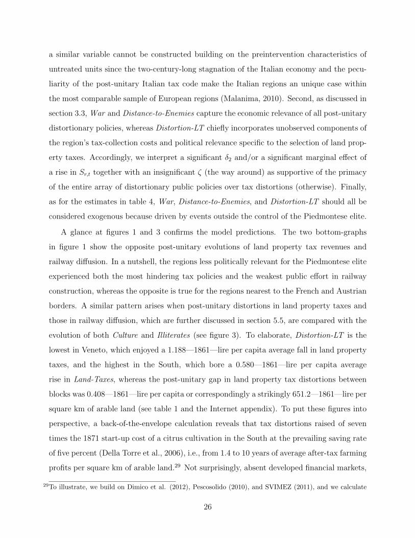
A glance at figures 1 and 3 confirms the model predictions. The two bottom-graphs

in figure 1 show the opposite post-unitary evolutions of land property tax revenues and

railway diffusion. In a nutshell, the regions less politically relevant for the Piedmontese elite

experienced both the most hindering tax policies and the weakest public effort in railway

construction, whereas the opposite is true for the regions nearest to the French and Austrian

borders. A similar pattern arises when post-unitary distortions in land property taxes and

those in railway diffusion, which are further discussed in section 5.5, are compared with the

evolution of both Culture and Illiterates (see figure 3). To elaborate, Distortion-LT is the

lowest in Veneto, which enjoyed a 1.188—1861—lire per capita average fall in land property

taxes, and the highest in the South, which bore a 0.580—1861—lire per capita average

rise in Land-Taxes, whereas the post-unitary gap in land property tax distortions between

blocks was 0.408—1861—lire per capita or correspondingly a strikingly 651.2—1861—lire per

square km of arable land (see table 1 and the Internet appendix). To put these figures into

perspective, a back-of-the-envelope calculation reveals that tax distortions raised of seven

times the 1871 start-up cost of a citrus cultivation in the South at the prevailing saving rate

of five percent (Della Torre et al., 2006), i.e., from 1.4 to 10 years of average after-tax farming

profits per square km of arable land.29 Not surprisingly, absent developed financial markets,

29To illustrate, we build on Dimico et al. (2012), Pescosolido (2010), and SVIMEZ (2011), and we calculate

26

the South was braked by this huge spike in investment costs and witnessed the sharpest fall

in a culture of cooperation and the most limited decline in illiteracy.

Multivariate analysis confirms these relationships (see table 5). As expected, the marginal

effects of a rise in War, δ2, and ζ are negative (positive if the dependent variable is Il-

literates) whenever significant. To illustrate, a one-standard-deviation rise in War—i.e.,

0.01—from its post-unitary mean—i.e., 0.005—corresponds to a 0.6-standard-deviation fall

in Culture and a one-standard-deviation increase in Illiterates. Similarly, a rise in Distance-

to-Enemies from the lowest North’s to the highest South’s value—1150 km—implies a 1.1-

standard-deviation decrease in Culture and a 1.7-standard-deviation fall in GSP, whereas

a one-standard-deviation increase in Distortion-LT or 1.8—1861—lire per capita leads to

a roughly 0.7-standard-deviation decrease (rise) in GDP, GSP, VA-T (Illiterates) and 1.4-

standard-deviation fall in VA-M. All these coefficients are significant at 10 percent or better.

5.4 Identifying Causal Relationships

Albeit reverse causation is not an issue (see sections 5.2 and 5.3), we cannot exclude that

our results are driven by unobserved heterogeneity and, in particular, by differences in 1861

structural conditions. To evaluate whether this is the case, we operate as follows. First, we

assess the impact of the initial structural dimensions on the estimates discussed in section

5.3. Next, we use selection on observables to assess the bias from unobservables.

5.4.1 Controlling for Observables

To illustrate the first exercise, we consider time dummies and their interaction with the

four dimensions displaying significantly different 1861 values in the South and in the North

(see table 2). Crucially, including decennial dummies also controls for another key time-

varying confounder, which is the series of end of the 19th century international shocks to

the terms of trade of the farming products discussed in section 2 (Barbagallo, 1980).

The first factor we consider is the average over the 1000-1850 period of the constraints

on the elite’s power developed by Tabellini (2010) and Boranbay and Guerriero (2016), i.e.,

that the average pretax farming profits per square km of arable land in Sicily were 5964 lire, which we takeas a proxy for the remainder of the South. Moreover, we use the fact that the average (distortions in) landproperty tax revenues per square km of arable land in the South were 565 (483) lire and that, being seed andlabor costs negligible, the main start-up expenses of a citrus cultivation were the five years of land propertytaxes to be payed while the newly planted trees became productive [Dimico et al. 2012, p. 2].

27

Democracy-I. Including this observable allows us to directly contrast our framework with

the aforementioned literature on the persistent effects of medieval political institutions on

present-day culture and outcomes (Putnam et al., 1993). The second structural condition

we analyze has been instead proposed by Del Monte and Pennacchio (2011), and it is defined

as the 1861 number of payers of land property taxes divided by the agricultural population

both collected from the “Inquiry into agriculture and peasant conditions” completed in 1885

by Stefano Jacini, i.e., Land-Fragmentation-I. Incorporating this control into equation (5)

directly tests the idea that inequality in land ownership and, more generally, power originated

an exploiter Southern bourgeoisie (Felice, 2014). We will obtain similar estimates should we

employ as proxy for power fragmentation the Gini coefficient proposed by Vecchi (2011).

Crucially, considering either Democracy-I or Land-Fragmentation-I makes also possible to

compare our model testable predictions with the alternative idea that the present-day divide

originates in the backwardness of the Kingdom of Two Sicilies (Franchetti and Sonnino,

1876) and/or the persistence of the Southern pre-unitary feudal system (Gramsci, 1966). To

understand instead the role of the variation in input availability on the asymmetric spread

of the Industrial Revolution (Krugman, 1981), we control for the 1861 coal price per tonne

in Genoa, which was the main harbor for its import, augmented for the transport cost to

the region in 1861 lire, i.e., Coal-Price-I. As clarified by Missiaia (2012), coal contributed

the most to the post-unitary power needs becoming increasingly pivotal in the success of

the industrial sectors. Exploiting instead variation in hydroelectric power, again available

from Missiaia (2012), delivers similar estimates. Finally, to explore the role of the initial

regional endowments of infrastructures, we include into our analysis the 1861 railway length

in km per square km, i.e., Railway-I. Crucially, using the predetermined values of these four

structural conditions minimizes the likelihood of their endogeneity.

Panels A to D of table 6 report the estimates of the specifications considering also time

dummies and their interaction with initial structural dimensions. Three are the key observa-

tions. First, our results remain qualitatively similar when we condition on observables sug-

gesting that, as discussed in more details in section 5.4.2, selection on unobservables should

not be considered an issue. Consistent with this remark, estimates available upon request

reveal that the time-variant impacts of the starting conditions are in general statistically

28

insignificant implying that alternative explanations of the opening of the present-day gap do

not make a dent in fitting the data. Second, the region’s taxation capacity is, conditional on

observables, the main driver of outcomes suggesting that it was the mix of all distortionary

policies to really matter. Finally, conditional on observables, distortionary policies do not

significantly shape VA-M. This pattern crucially implies that extraction did not allow the

Northern growth sector to start its chase to the most advanced European industries as the

prewar divide clearly suggests [Pescosolido 2014, p. 278-300]. Hence, post-unitary distor-

tions cannot be considered the acceptable price that the low political relevance regions had

to pay for the industrialization of the only part of the country ready for it and, in turn, of

Italy (Romeo, 1987).30 This conclusion squares with proposition 2 whereby a sufficient rise

in the rulers’ extractive power penalizes all low political relevance regions.

5.4.2 Using Selection on Observables to Assess the Bias from Unobservables

Despite our attempts to control for observables, our estimates may still be biased by un-

observables correlated with the regional productivity, the region’s taxation capacity, and/or

its political relevance. To evaluate this issue, we calculate the index proposed by Oster

(2016) to measure how much stronger selection on unobservables, relative to selection on

observables, must be to explain away the entire estimated effect. To see how it is calculated,

consider a regression with a restricted set of control variables and one with a full set of

controls. Next, denote the estimate of the coefficient attached to the variable of interest

and the R2 from the first regression λR and RR, where R stands for “restricted,” and those

from the second regression λF and RF , where F stands for “full.” Then, the index is the

absolute value of λF (RF−RR)(λR−λF )(1−RF )

. The intuition behind the formula is as follows. The lower

the absolute value of (λR − λF ) is and the nearer RF is to its maximum value of 1, the less

the estimate of the coefficient attached to the variable of interest is affected by selection on

observables, and the stronger selection on unobservables needs to be to explain away the

entire effect. Moreover, the higher the absolute value of λF and RF −RR are, the greater is

the effect that needs to be explained away by selection on unobservables.

In table 7, we focus on the variables testing the key model predictions, i.e., the proxy for

30To illustrate, the divide “was not deliberately constructed [. . . ] to the disadvantage of the South, but it waseven acceptable in a country [with a differentiated] productive system” [Iuzzolino et al. 2011, p. 26].

29

the productivity of arboriculture and the measure of the regional political relevance in the

endogenous taxation models run respectively on the pre-unitary and post-unitary samples

(see columns (1) and (2)), and War, War 2, Distance-to-Enemies, and Distortion-LT in the

outcome equations (see columns (3) to (8)). The covariates incorporated only in the full set

are listed in the last three lines of table 7 and include in the case of the outcome regressions

the time effects and their interaction with Democracy-I since these are the most relevant

extra controls in table 6. We will obtain similar indexes (available upon request), should we

focus instead on one among Land-Fragmentation-I, Coal-Price-I, and Railway-I. The median

and the average of the indexes in columns (1) and (2) are 0.72 and 0.96, whereas those in

columns (3) to (8) are 1.09 and 3.89. Thus, to attribute the entire OLS estimates to selection

effects, on average selection on unobservables would have to be about 4 times greater than

selection on observables. Given the very high fit of our regressions—i.e., with an average

within R2 of 0.31(0.47) in table 4(5) and 0.75 in panel A of table 6, this is unreasonable.

5.5 Endogenous Public Good Provision

We close our analysis by assessing whether distortions in taxation were accompanied by

similar distortions in public spending. To elaborate, we build on our model, and we first

identify the pre-unitary determinants of railway diffusion and we then assess its post-unitary

distortions by estimating public good provision equations of the following type

Rr,t = αr + ιt + β′3Ar,t + β′4A2r,t + γ4Sr,t + γ5S

2r,t + δ3Pr,t + δ4P

2r,t + τ0Orιt + ηr,t, (6)

where Rr,t is the length in km per square km of railway built in the previous decade, i.e.,

Railway. Following Picci (2002), we also consider the orographic nature of each region as a

proxy for railway building costs by including in the specification the terrain ruggedness Or

in km—i.e., Ruggedness—interacted with time dummies ιt. Since ιt appears also as extra

control, we do not cluster standard errors at the regional level to preserve a sufficient within-

region variation. This time, αr accounts for time-invariant shifters of railway diffusion like

the traveling distance from international markets and long-lasting institutions.

Table 8 is structured in the same way as table 4 and reveals the following two facts. First,

the crucial aim of pre-unitary railway diffusion was the strengthening of the export of farming

30

products and, in particular, wheat in Lombardy-Venetia, which because of the support of

Vienna was the only Italian state outside the Kingdom of Sardinia with any public spending

capacity [Pescosolido 2014, p. 38 and 100]. Accordingly, a rise in Wheat from the lowest

South’s value—i.e., 0 in Calabria—to the highest North’s one—i.e., 0.87 in Lombardy—

implies a huge 42.8-standard-deviation increase in Railway in column (1) and is always

significant at 5 percent in columns (1) to (3). Second, the post-unitary railway expansion

was only shaped by the regional political relevance. In particular, a rise in Distance-to-

Enemies from the lowest North’s value to the highest South’s value—1150 km—leads to a

7.6-standard-deviation fall in Railway, which is significant at 5 percent (see column (6)).

Placing side to side these with the estimates discussed above, we can conclude that

regions farther away from the possible battlefields enjoyed the slowest post-unitary railway

diffusion but paid the highest relative costs. Moreover, plotting the differences between

the observed post-unitary values of Railway and those forecasted using the specification in

column (1) of table 8—i.e., Distortion-R—across regional clusters reveals that both low and

middle political relevance regions experienced periods of both under- and over-investment

in railway, whereas the state’s effort in the high political relevance region was generally

more intense than it would have been without unification (see upper-right graph in figure

3). This evidence is consistent with the conclusions we draw in section 5.4 insofar it speaks

again against the idea that subsidization of the Northern infrastructures at the South’s

expenses was optimal. On the one hand indeed, the unitary government failed to provide

the South with the technical means to replace the foreign markets with domestic outlets in the

aftermath of the price shocks of the 1880s further squeezing the after tax profits to be invested

in the industry [Iuzzolini et al. 2011, p. 20]. On the other hand, to effectively strengthen

the newborn advanced manufacturing industry the highest railway spending should have

targeted the middle and not the high political relevance regions [Iuzzolini et al. 2011, p. 22].

5.6 External Validity

To alleviate concerns that the Italian unification might be a special case, we briefly

discuss the closely related case of the post-Civil War divide between Southern and Northern

US states, which we illustrate in more details in the Internet appendix.

31

In the 1850s, slavery was source of mounting political tension between the Southern slave

states and the abolitionist North, and accordingly the Republicans, dominant in the North,

built the entire 1860 Lincoln’s presidential campaign on a complete ban on slave-owning.

Lincoln’s election was then the final trigger to the secession of eleven Southern states first

and a dreadful conflict between them and the rest of the Union then. The war brought about

almost one million casualties, the murder of Lincoln, and the tacit understanding among

the winners that the “prewar leadership of the Southern slavocrats in national politics was

permanently to be replaced in favor of the Northern direction” [Donald and Randall 1961,

p. 535]. To this end, the new government first split the ex-Confederate states into five

military districts under martial law and then steadily raised their property taxes to force

redistribution of land from those white planters that, because of the heavier tax burden,

were going to be expropriated of their estates to blacks and poor whites [Foner 1988, p. 346-

383]. Yet, because of this last group’s liquidity constraints, Southern land were increasingly

acquired by Northern landowners greatly widening the development gap between the two

blocks [Foner 1988, p. 399]. Similarly to the Italian case, the Southern rage together with the

Northern population’s discontent with political instability irremediably put an end, after the

Democrats’ victory of the disputed 1876 presidential election, to extraction but only when

its consequences were already permanent [Donald and Randall 1961, p. 548].

6 Conclusions

This paper has developed a theory of “endogenous extractive policies” grounded on the

mix of the heterogeneity in the relevance of the dominated groups for the dominating one

and changes in the rulers’ extractive power. Crucially, our framework helps shed new light

on a key issue in economics, which is the huge divide between North and South of Italy

despite more than 150 years of common formal institutions. In particular, we document that

its opening is the result of the region-specific policies selected between 1861 and 1911 by

the elite of the Kingdom of Sardinia, which annexed the rest of Italy in 1861. To illustrate,

pre-unitary land property taxes and railway diffusion were shaped by each region’s farming

productivity but not by its political relevance for the Piedmontese elite, whereas the opposite

was true for post-unitary ones. Moreover, post-unitary tax distortions and the severity of

32

the remaining extractive policies—captured by the region’s taxation capacity and political

relevance—determined the North-South gaps in culture, literacy, and development but not

that in the manufacturing industry value added. Together these two patterns imply that

extraction cannot be considered the acceptable price for the Italian development since it

neither eased the formation of an unitary market nor favored industrialization.

Since our proxies for the drivers of extraction are independent of the policy-makers’ will,

reverse causation is not an issue. Yet, our results could still be produced by unobserved

heterogeneity. To evaluate this aspect, we follow a two-step strategy. First, we document

that our estimates remain robust to the consideration of both fixed region and time effects and

the structural conditions differentiating the two blocks in 1861, i.e., pre-unitary inclusiveness

of political institutions, land ownership fragmentation, coal price, and the railway length.

Second, we build on Oster (2016), and we calculate that on average selection on unobservables

would have to be about 4 times greater than selection on observables to completely explain

away our results. Given the very high fit of our regressions, this is unlikely.

Our results characterize the crack of the dawn of the North-South divide, and identifying

more recent factors aggravating these disparities is a key avenue for further research [Iuzzolino

et al. 2011 p. 7-10]. More important, our framework can be employed to study related cases

as the deep conflicts that are shaking the EU nowadays (see also Guiso et al., [2015]).

33

References

Abadie, Alberto, and Javier Gardeazabal. 2003. “The Economic Costs of Conflict: A Case

Study of the Basque Country.” American Economic Review, 93: 113-132.

Abadie, Alberto, Alexis Diamond, and Jens Hainmueller. 2015. “Comparative Politics and

the Synthetic Control Method.” American Journal of Political Science, 59: 495-510.

Acemoglu, Daron, and James Robinson. 2012. Why Nations Fail: The Origins of Power,

Prosperity, and Poverty. New York, NY: Crown Publishers.

Alesina, Alberto, and Enrico Spolaore. 2005. “War, Peace, and the Size of Countries.”

Journal of Public Economics, 89: 1333-1354.

Andersen, Thomas B., Jeanet Bentzen, Carl-Johan Dalgaard, Paul Sharp. 2016. “Pre-

Reformation Roots of the Protestant Ethic.” Forthcoming Economic Journal.

Baffigi, Alberto. 2011.“Italian National Accounts.” Economic History Working Papers,

Banca d’Italia, n. 18.

Barbagallo, Francesco. 1980. Mezzogiorno e Questione Meridionale (1860-1980). Napoli:

Guida Editori.

Barkow, Jerome H., Leda Cosmides, and John Tooby. 1992. The Adapted Mind: Evolu-

tionary Psychology and the Generation of Culture. New York, NY: Oxford University

Press.

Besley, Timothy, and Torsten Persson. 2009. “The Origins of State Capacity: Property

Rights, Taxation, and Politics.” American Economic Review, 99: 1218-1244.

Besley, Timothy, and Hannes Mueller. 2012. “Estimating the Peace Dividend: The Impact

of Violence on House Prices in Northern Ireland.” American Economic Review, 102:

810-833.

Boranbay, Serra, and Carmine Guerriero. 2016. “Endogenous (In)Formal Institutions.”

Unpublished.

34

Cafagna, Luciano. 1989. Dualismo e Sviluppo nella Storia d’Italia. Venezia: Marsilio

Editore.

Cameron, A. Colin, and Douglas L. Miller. 2015. “A Practitioner’s Guide to Cluster-Robust

Inference.” Journal of Human Resources, 50: 317-373.

Ciccarelli, Carlo, and Stefano Fenoaltea. 2013. “Through the Magnifying Glass: Provincial

Aspects of Industrial Growth in Post-unitary Italy.” The Economic History Review, 66:

57-85.

Clark, Gregory. 2005. A Farewell to Alms. Princeton, NJ: Princeton University Press.

Cohen, Jon and Giovanni Federico. 2003. The Growth of the Italian Economy, 1820-1960.

Cambridge, MA: Cambridge University Press.

Conley, Tim G. 1999. “GMM Estimation With Cross Sectional Dependence.” Journal of

Econometrics, 92: 1-45.

Corbetta, Piergiorgio, and M. Serena Piretti. 2008. Atlante Storico-elettorale d’Italia (1861-

2006). Bologna: Zanichelli.

Della Torre, Giuseppe, Mimı Coccıa, Valentina De Leonardis, Maria Carmela Schisani. 2006.

“La Crescita del Sistema Finanziario Italiano dopo l’Unificazione Politica, 1861-1914:

Financial Deepening e/o Errori Statistici e Metodologici?” Unpublished.

Del Monte, Alfredo, and Luca Pennacchio. 2011. “The Structure of Agricultural Production

and the Causes of Brigandage and Criminal Organisations in Italy after Unification:

Theory and Evidence.” Unpublished.

Dimico, Arcangelo, Alessia Isopi, and Ola Olsson. 2012. “Origins of the Sicilian Mafia: The

Market for Lemons.” Unpublished.

Dincecco, Mark, Giovanni Federico, and Andrea Vindigni. 2011. “Warfare, Taxation, and

Political Change: Evidence from the Italian Risorgimento.” Journal of Economic History,

71: 887-914.

35

Donald, David H., and James G. Randall. 1961. The Civil War and Reconstruction. Boston,

MA: D.C. Heath and Company.

Duggan, Christopher. 2008. The Force of Destiny: A History of Italy since 1796. New York,

NY: Houghton Mifflin Company.

Duggan, Christopher. 2014. A Concise History of Italy. Cambridge, UK: Cambridge Uni-

versity Press.

Esposto, Alfredo G. 1997. “Estimating Regional per Capita Income: Italy 1861-1914.”

Journal of European Economic History, 26: 585-604.

Federico, Giovanni. 2007. “Ma l’Agricoltura Meridionale Era Davvero Arretrata?” Rivista

di Politica Economica, 97: 317-340.

Federico, Giovanni. 2009. An Economic History of the Silk Industry, 1830-1930. Cambridge,

MA: Cambridge University Press.

Felice, Emanuele. 2012. “Regional Convergence in Italy, 1891-2001: Testing Human and

Social Capital.”Cliometrica, 6: 267-306.

Felice, Emanuele. 2014. Perche il Sud e Rimasto Indietro. Bologna: Il Mulino.

Foner, Eric. 1988. Reconstruction: America’s Unfinished Revolution, 1863-1877. New York,

NY: Harper & Row.

Franchetti, Leopoldo, and Sidney Sonnino. 1876. La Sicilia nel 1876. Siena: Barbera.

Frascani, Paolo. 1988. Finanza, Economia ed Intervento Pubblico dall’Unificatione agli Anni

Trenta. Napoli: Istituto Italiano per gli Studi Filosofici.

Galor, Oded. 2011. Unified Growth Theory. Princeton, NJ: Princeton University Press.

Gramsci, Antonio. 1966. La Question Meridionale. Roma: Editori Riuniti.

Guerriero, Carmine. 2016. “Endogenous Institutions and Economic Outcomes.” Unpub-

lished.

36

Guiso, Luigi, Helios Herrera, and Massimo Morelli. 2015. “Cultural Differences and Institu-

tional Integration.” Journal of International Economics, 99: S97-S113.

Guiso, Luigi, Paola Sapienza, and Luigi Zingales. 2016. “Long-Term Persistence.” Journal

of the European Economic Association, 14: 1401-1436.

Iuzzolino, Giovanni, Guido Pellegrini, and Gianfranco Viesti. 2011. “Convergence Among

Italian Regions, 1861-2011.” Bank of Italy Economic History Working Papers, 22.

Jacini, Stefano. 1885. Atti della Giunta per la Inchiesta Agraria sulle Condizioni della

Classe Agricola 1882-1885. Sala Bolognese: Forni.

Killinger, Charles L. 2002. The History of Italy. Westport, CT: Greenwood Press.

Krugman, Paul. 1981.“Trade, Accumulation, and Uneven Development.”Journal of Devel-

opment Economics, 8: 149-161.

Luterbacher, Jurg, Daniel Dietrich, Elena Xoplaki, Martin Grosjean, and Heinz Wanner.

2004. “European Seasonal and Annual Temperature Variability, Trends, and Extremes

Since 1500.” Science, 303: 1499-1503.

Malanima, Paolo. 2006. “An Age of Decline. Product and Income in Eighteenth-Nineteenth

Century Italy.” Rivista di Storia Economica, 21: 91-133.

Malanima, Paolo. 2010. “The Long Decline of a Leading Economy: GDP in Central and

Northern Italy, 1300-1913.” European Review of Economic History, 15: 169-219.

Ministero dell’Agricoltura, Industria e Commercio. 1864, 1878, 1881, 1890, 1892, 1900, 1912.

Annuario Statistico Italiano. Roma: Tipografia Nazionale Bertero.

Ministero delle Finanze del Regno d’Italia. 1863, 1872, 1882, 1888. Annuario del Ministero

delle Finanze del Regno d’Italia. Torino: Stamperia Reale.

Missiaia, Anna. 2012. “Market vs. Endowment: Explaining Early Industrial Location in

Italy (1871-1911).” Unpublished.

37

Nitti, Francesco Saverio. 1993. Nord e Sud. Rionero in Vulture: Calice Editori.

North, Douglass C., John J. Wallis, Barry R. Weingast. 2009. Violence and Social Orders:

A Conceptual Framework for Interpreting Recorded Human History. Cambridge, UK:

Cambridge University Press.

Oster, Emily F. 2016. “Unobservable Selection and Coefficient Stability: Theory and Vali-

dation.” Forthcoming, Journal of Business Economics and Statistics.

Paoletti, Ciro. 2008. A Military History of Italy. Westport, CT: Praeger Security Interna-

tional.

Parravicini, Giannino. 1958. La Politica Fiscale e le Entrate Effettive del Regno d’Italia

1860-1890. Turin: ILTE.

Pauling, Andreas, Jurg Luterbacher, Carlo Casty, and Heinz Wanner. 2006. “Five Hundred

Years of Gridded High Resolution Precipitation Reconstructions Over Europe and the

Connection to Large-scale Circulation.” Climate Dynamics, 26: 387-405.

Pescosolido, Guido. 2010. “L’Economia Siciliana nell’Unificazione Italiana.” Mediterranea.

Ricerche Storiche, 19: 219-234.

Pescosolido, Guido. 2011. “La Costruzione dell’Economia Unitaria.” In Enciclopedia Ital-

iana, ed., Roma: Treccani.

Pescosolido, Guido. 2014. Unita Nazionale e Sviluppo Economico 1750-1913. Roma: Edi-

zioni Nuova Cultura.

Petrusewicz, Marta. 1996. Latifundium: Moral Economy and Material Life in a European

Periphery. Ann Arbor, MI: University of Michigan Press.

Picci, Lucio. 2002. “Le Opere Pubbliche dall’Unita d’Italia: l’Informazione Statistica.”

Rivista di Politica Economica, 92: 29-80.

Putnam, Robert, Robert Leonardi, and Raffaella Nanetti. 1993. Making Democracy Work.

New York, NY: Simon & Schuster.

38

Riall, Lucy. 2009. Risorgimento: The History of Italy from Napoleon to Nation State.

London: Palgrave Macmillan.

Romani, Mario. 1982. Storia Economica d’Italia nel Secolo XIX, 1815-82. Bologna: Il

Mulino.

Romeo, Rosario. 1987. L’Italia Liberale: Sviluppo e Contraddizioni. Milano: Il Saggiatore.

Rosenthal, Howard, and Erik Voeten. 2007. “Measuring Legal Systems.” Journal of Com-

parative Economics, 35: 711-728.

Salvemini, Gaetano. 1963. Movimento Socialista e Questione Meridionale. Milano: Fel-

trinelli.

Sereni, Emilio. 1947. Il Capitalismo nelle Campagne (1860-1900). Torino: Einaudi.

SVIMEZ. 2011. 150 Anni di Statistiche Italiane: Nord e Sud. 1861-2011. Bologna: Il

Mulino.

Tabellini, Guido. 2010. “Culture and Institutions: Economic Development in the Regions

of Europe.” Journal of the European Economic Association, 8: 677-716.

Vecchi, Giovanni. 2011. In Ricchezza e in Poverta. Il Benessere Degli Italiani dall’Unita a

Oggi. Bologna: Il Mulino.

Zamagni, Vera. 1980. “The Rich in a Late Industrializer: The Case of Italy, 1800-1945.”

In Wealth and the Wealthy in the Modern World, ed. William D. Rubinstein. London:

Croom Helm.

Zamagni, Vera. 1993. The Economic History of Italy 1860-1990. New York, NY: Oxford

University Press.

39

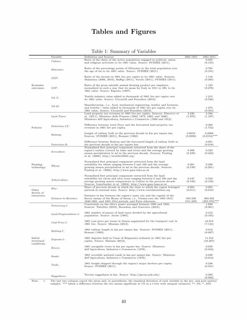
Tables and Figures

Table 1: Summary of VariablesVariable Definition and Sources 1801-1851 1861-1911

Culture:Ratio of the share of the active population engaged in political, union, 0.935and religious activities to its 1861 value. Source: SVIMEZ (2011). (0.155)

Illiterates:Ratio of the percentage points of illiterates in the total population over 0.784the age of six to its 1861 value. Source: SVIMEZ (2011). (0.191)

GDP:Ratio of the income in 1861 lire per capita to its 1861 value. Sources: 1.118Malanima (2006, 2010), Baffigi (2011), Vecchi (2011), SVIMEZ (2011). (0.285)

Economic Ratio of the gross saleable annual farming product per employee, 1.123outcomes: GSP: normalized in such a way that its mean for Italy in 1911 is 100, to its (0.278)

1861 value. Source: Esposto (1997).

VA-T :Textile industry value added in thousands of 1861 lire per capita over 1.213its 1861 value. Source: Ciccarelli and Fenoaltea (2013). (0.526)

VA-M :Manufacturing—i.e., food, mechanical engineering, leather and footwear,and textiles—value added in thousands of 1861 lire per capita over its 1.2731861 value. Source: Ciccarelli and Fenoaltea (2013). (0.354)Land property tax revenues in 1861 lire per capita. Sources: Dincecco et 3.236 3.590

Land-Taxes: al. (2011), Ministero delle Finanze (1863, 1872, 1882, and 1888), (1.970) (1.187)Ministero dell’Agricoltura, Industria e Commercio (1900 and 1912).

Distortion-LT :Difference between Land-Taxes and the forecasted land property tax 0.360

Policies: revenues in 1861 lire per capita. (1.752)

Railway:Length of railway built in the previous decade in km per square km. 0.0016 0.0089Sources: SVIMEZ (2011), Romani (1982). (0.0036) (0.0152)***

Difference between Railway and the forecasted length of railway built in 0.001Distortion-R: the previous decade in km per square km. (0.018)

Sericulture:

Normalized first principal component extracted from the share of theregion’s surface covered by lakes and rivers and the average growing 0.306 0.323season precipitation in ml in the previous decade. Sources: Pauling (0.239) (0.243)et al. (2006), http://worldwildlife.org/

Wheat:

Normalized first principal component extracted from the landFarming suitability for wheat ranging between 0 and 100 and the average 0.281 0.298technology: growing season precipitation in ml in the previous decade. Sources: (0.199) (0.201)

Pauling et al. (2006), http://www.gaez.iiasa.ac.at

Arboriculture:

Normalized first principal component extracted from the landsuitability for citrus and olive trees ranging between 0 and 100 and the 0.547 0.532average growing season temperature in Celsius in the previous decade. (0.192) (0.192)Sources: Luterbacher et al. (2004), http://www.gaez.iiasa.ac.at

War :Share of previous decade in which the state to which the region belonged 0.004 0.005

Other partook in external wars. Source: http://www.correlatesofwar.org (0.011) (0.010)drivers ofextraction: Distance in km between the region’s main city and the capital of the

Distance-to-Enemies: fiercer enemy of the House of Savoy, i.e., Vienna over the 1801-1813, 934.539 803.4621848-1881, and 1901-1914 periods, and Paris otherwise. (311.239) (255.570)***

Democracy-I :Constraints on the elite’s power averaged between 1000 and 1850. 1.838Sources: Tabellini (2010), Boranbay and Guerriero (2016). (0.961)

Land-Fragmentation-I :1861 number of payers of land taxes divided by the agricultural 0.412population. Source: Jacini (1885). (0.165)

Coal-Price-I :1861 coal price per tonne in Genoa augmented for the transport cost in 44.0191861 lire. Source: Missiaia (2012). (7.144)

Railway-I :1861 railway length in km per square km. Sources: SVIMEZ (2011), 0.012Romani (1982). (0.007)

InitialDeposits-I :

1861 deposits held in Casse di Risparmio ordinarie in 1861 lire per 11.310structural capita. Source: Missiaia (2012). (16.267)conditions:

Rivers:1861 navigable rivers in km per square km. Source: Ministero 0.059dell’Agricoltura, Industria e Commercio (1878). (0.052)

Roads:1861 accesible national roads in km per square km. Source: Ministero 0.028dell’Agricoltura, Industria e Commercio (1878). (0.014)

Trade:1861 freight shipped through the region’s major harbors per capita. 0.248Source: SVIMEZ (2011). (0.351)

Ruggedness:Terrain ruggedness in km. Source: http://gecon.yale.edu/ 0.292

(0.082)

Note: 1. The last two columns report the mean and, in parentheses, the standard deviation of each variable in the pre- and post-unitarysamples. *** labels a difference between the two means significant at 1% in a t-test with unequal variances; **, 5%; *, 10%.

40

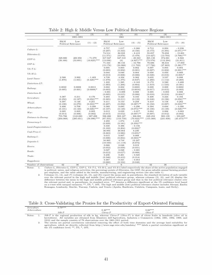
Table 2: High & Middle Versus Low Political Relevance Regions(1) (2) (3) (4) (5) (6) (7) (8) (9)

1801-1851 1861 1861-1911

H&M Low(1) - (2)

H&M Low(4) - (5)

H&M Low(7) - (8)

Political Relevance Political Relevance Political Relevance

Culture-L:0.757 1.017 - 0.260 0.712 0.950 - 0.238

(0.207) (0.343) (0.160) (0.173) (0.394) (0.071)***

Illiterates-L:74.514 82.933 - 8.419 55.057 70.858 - 15.801

(11.571) (8.079) (5.478) (19.427) (13.703) (3.768)***

GDP-L:329.880 400.958 - 71.079 317.947 347.510 - 29.563 365.138 374.061 - 8.922(39.160) (53.891) (10.825)*** (13.036) (0) (4.927)*** (72.579) (112.294) (21.811)

GSP-L:71.343 88.133 - 16.790 78.686 96.644 - 17.959

(15.176) (24.988) (11.703) (17.726) (27.803) (5.381)***

VA-T-L:0.005 0.003 0.002 0.007 0.003 0.004

(0.003) (0.002) (0.001) (0.007) (0.002) (0.001)***

VA-M-L:0.044 0.040 0.004 0.058 0.050 0.009

(0.013) (0.008) (0.006) (0.028) (0.016) (0.005)*

Land-Taxes:2.588 3.992 - 1.403 4.739 4.356 0.382 3.635 3.537 0.098

(1.870) (1.831) (0.420)*** (1.678) (1.375) (0.847) (1.260) (1.112) (0.269)

Distortion-LT :1.222 1.385 - 0.163 0.172 0.580 - 0.408

(1.683) (1.206) (0.804) (1.919) (1.533) (0.391)

Railway:0.0022 0.0008 0.0013 0.002 0.002 0.0003 0.009 0.009 0.0002(0.005) (0.001) (0.0008)* (0.003) (0.003) (0.0016) (0.017) (0.013) (0.003)

Distortion-R:- 0.001 - 0.009 0.008 0.005 - 0.003 0.008(0.005) (0.015) (0.006) (0.018) (0.019) (0.004)*

Sericulture:0.387 0.211 0.176 0.403 0.220 0.183 0.408 0.224 0.184

(0.250) (0.187) (0.050)*** (0.265) (0.211) (0.132) (0.248) (0.196) (0.050)***

Wheat:0.397 0.146 0.251 0.411 0.153 0.258 0.419 0.158 0.262

(0.198) (0.079) (0.033)*** (0.207) (0.092) (0.087)** (0.192) (0.087) (0.033)***

Arboriculture:0.408 0.708 - 0.299 0.389 0.685 - 0.296 0.394 0.694 - 0.300

(0.101) (0.140) (0.028)*** (0.107) (0.149) (0.073)*** (0.100) (0.139) (0.028)***

War :0.005 0.003 0.003 0.012 0.029 - 0.017 0.004 0.006 - 0.003

(0.014) (0.006) (0.002) (0.013) (0.012) (0.007)** (0.007) (0.012) (0.002)

Distance-to-Enemy:755.786 1143.083 - 387.298 596.286 903.167 - 306.881 649.452 983.139 - 333.687

(204.068) (285.051) (56.996)*** (87.355) (153.750) (70.922)*** (155.368) (231.839) (45.473)***

Democracy-I :2.492 1.074 1.418

(0.929) (0.181) (0.359)***

Land-Fragmentation-I :0.340 0.496 - 0.156

(0.102) (0.204) (0.092)*

Coal-Price-I :46.894 40.664 6.230(8.663) (3.980) (3.655)*

Railway-I :0.015 0.007 0.008

(0.008) (0.004) (0.003)**

Deposits-I :16.963 4.716 12.247

(19.550) (11.119) (8.672)

Rivers:0.068 0.048 0.019

(0.052) (0.059) (0.031)

Roads:0.027 0.028 - 0.001

(0.012) (0.017) (0.008)

Trade:0.236 0.261 - 0.025

(0.348) (0.412) (0.214)

Ruggedness:0.267 0.321 - 0.054

(0.060) (0.104) (0.048)Number of observations 42 36 7 6 42 36

Notes: 1. Culture-L, Illiterates-L, GDP-L, GSP-L, VA-T-L, VA-M-L, and VA-E-L label respectively the share of the active population engagedin political, union, and religious activities, the percentage points of illiterates, the GDP, the gross saleable annual farming productper employee, and the value added in the textile, manufacturing, and engineering sectors (see also table 1).

2. Columns (1), (4), and (7) (columns (2), (5), and (8)) report the mean and, in parentheses, the standard deviation of each variableover the relevant period in the high and middle (low) political relevance group, whereas columns (3), (6), and (9) display thedifference between the mean in the high and middle political relevance group and that in the low political relevance cluster overthe relevant period and, in parentheses, its standard error. *** denotes a difference significant at the 1% confidence level basedon a t-test with unequal variances; **, 5%; *, 10%. The high and middle (low) political relevance cluster includes Abruzzi, EmiliaRomagna, Lombardy, Marche, Tuscany, Umbria, and Veneto (Apulia, Basilicata, Calabria, Campania, Lazio, and Sicily).

Table 3: Cross-Validating the Proxies for the Productivity of Export-Oriented FarmingSericulture 0.79***Arboriculture 0.46*** 0.66***

Silk-P Citrus-P Olive-P

Notes: 1. Silk-P is the regional production of silk in kg, whereas Citrus-P (Olive-P) is that of citrus fruits in hundreds (olive oil inhectoliters). All variables are obtained from Ministero dell’Agricoltura, Industria e Commercio (1864, 1881, 1892, 1900, and1912) and the sample consists of 78 observations over the 1861-1911 period.

2. The entries are partial correlations calculated removing the effect of both time dummies and the average land suitability foragriculture, which we directly collected from http://www.sage.wisc.edu/iamdata/ *** labels a partial correlation significant atthe 1% confidence level; **, 5%; *, 10%.

41

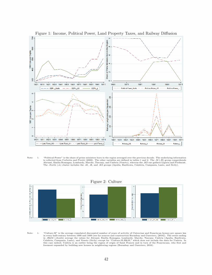
Figure 1: Income, Political Power, Land Property Taxes, and Railway Diffusion

Note: 1. “Political-Power” is the share of prime ministers born in the region averaged over the previous decade. The underlying informationis collected from Corbetta and Piretti (2008). The other variables are defined in tables 1 and 2. The M ( H) group comprehendsAbruzzi, Emilia Romagna, Lombardy, Marche, Tuscany, and Umbria (Veneto), whereas the KS one gathers Liguria and Piedmont.The North ( L) cluster includes the M, H, and KS groups (Apulia, Basilicata, Calabria, Campania, Lazio, and Sicily).

Figure 2: Culture

Note: 1. “Culture-M” is the average cumulated discounted number of years of activity of Cistercian and Franciscan houses per square kmin every half-century between 1000 and 1600 (see for sources and construction Boranbay and Guerriero, [2016]). The series endingin H&M ( South) average the values for Abruzzi, Emilia Romagna, Lombardy, Marche, Tuscany, Umbria (Apulia, Basilicata,Calabria, Campania, Lazio), and Veneto (Sicily) except for “Culture-M H&M,” which does not include the data for Umbria. Inthis case indeed, Umbria is an outlier being the region of origin of Saint Francis and in turn of the Franciscans, who first andforemost expanded by building new houses in neighboring regions (Boranbay and Guerriero, 2016).

42

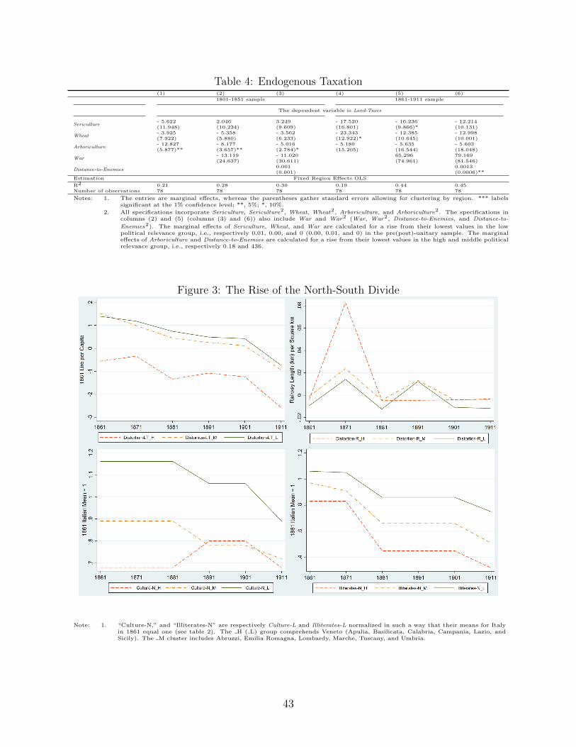
Table 4: Endogenous Taxation(1) (2) (3) (4) (5) (6)

1801-1851 sample 1861-1911 sample

The dependent variable is Land-Taxes

Sericulture- 5.622 2.046 3.249 - 17.520 - 16.236 - 12.214(11.948) (10.234) (9.609) (16.801) (9.866)* (10.131)

Wheat- 3.925 - 5.358 - 3.562 - 23.343 - 12.385 - 12.998(7.922) (5.880) (6.233) (12.922)* (10.645) (10.001)

Arboriculture- 12.827 - 8.177 - 5.016 - 5.180 - 5.635 - 5.603(5.877)** (3.657)** (2.784)* (15.205) (16.544) (18.048)

War- 13.119 - 11.020 65.296 79.169(24.637) (30.611) (74.961) (81.546)

Distance-to-Enemies0.001 0.0013(0.001) (0.0006)**

Estimation Fixed Region Effects OLS

R2 0.21 0.28 0.30 0.19 0.44 0.45Number of observations 78 78 78 78 78 78

Notes: 1. The entries are marginal effects, whereas the parentheses gather standard errors allowing for clustering by region. *** labelssignificant at the 1% confidence level; **, 5%; *, 10%.

2. All specifications incorporate Sericulture, Sericulture2, Wheat, Wheat2, Arboriculture, and Arboriculture2. The specifications incolumns (2) and (5) (columns (3) and (6)) also include War and War2 (War, War2, Distance-to-Enemies, and Distance-to-

Enemies2). The marginal effects of Sericulture, Wheat, and War are calculated for a rise from their lowest values in the lowpolitical relevance group, i.e., respectively 0.01, 0.00, and 0 (0.00, 0.01, and 0) in the pre(post)-unitary sample. The marginaleffects of Arboriculture and Distance-to-Enemies are calculated for a rise from their lowest values in the high and middle politicalrelevance group, i.e., respectively 0.18 and 436.

Figure 3: The Rise of the North-South Divide

Note: 1. “Culture-N,” and “Illiterates-N” are respectively Culture-L and Illiterates-L normalized in such a way that their means for Italyin 1861 equal one (see table 2). The H ( L) group comprehends Veneto (Apulia, Basilicata, Calabria, Campania, Lazio, andSicily). The M cluster includes Abruzzi, Emilia Romagna, Lombardy, Marche, Tuscany, and Umbria.

43

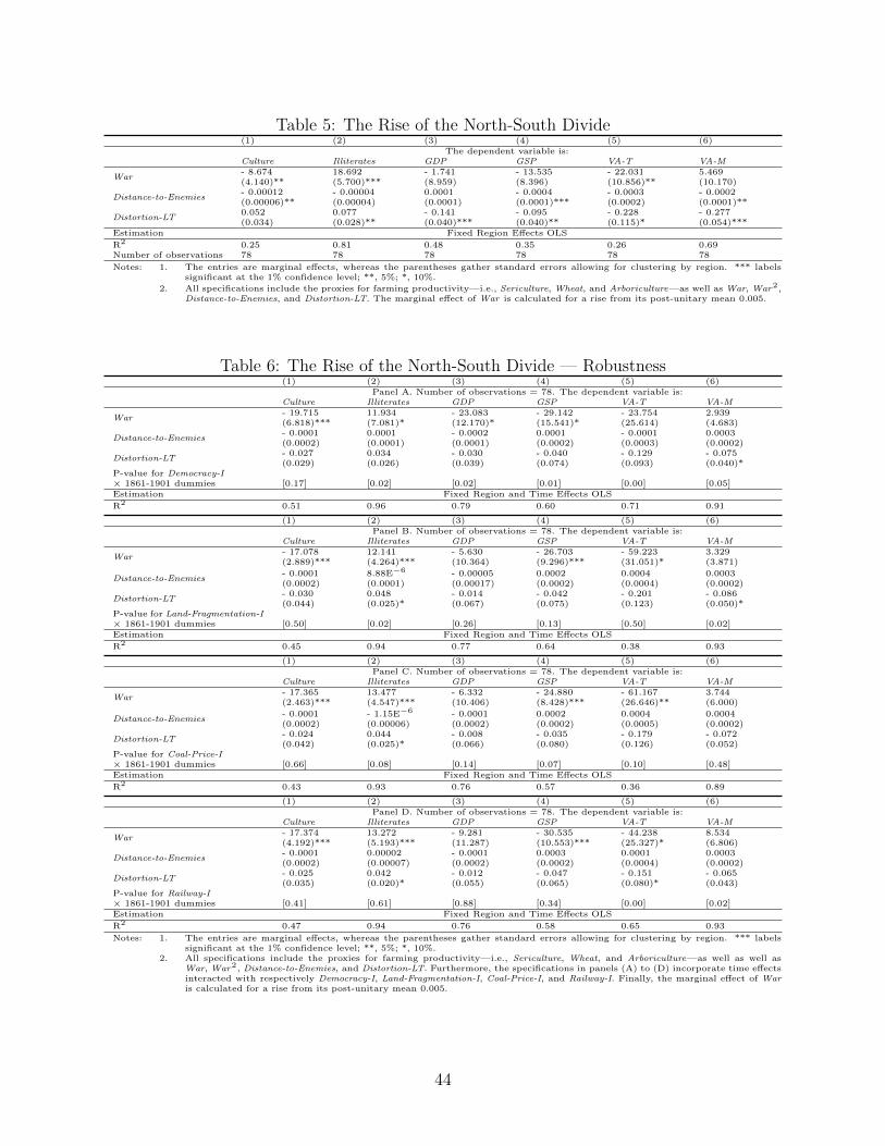
Table 5: The Rise of the North-South Divide(1) (2) (3) (4) (5) (6)

The dependent variable is:Culture Illiterates GDP GSP VA-T VA-M

War- 8.674 18.692 - 1.741 - 13.535 - 22.031 5.469(4.140)** (5.700)*** (8.959) (8.396) (10.856)** (10.170)

Distance-to-Enemies- 0.00012 - 0.00004 0.0001 - 0.0004 - 0.0003 - 0.0002(0.00006)** (0.00004) (0.0001) (0.0001)*** (0.0002) (0.0001)**

Distortion-LT0.052 0.077 - 0.141 - 0.095 - 0.228 - 0.277(0.034) (0.028)** (0.040)*** (0.040)** (0.115)* (0.054)***

Estimation Fixed Region Effects OLS

R2 0.25 0.81 0.48 0.35 0.26 0.69Number of observations 78 78 78 78 78 78

Notes: 1. The entries are marginal effects, whereas the parentheses gather standard errors allowing for clustering by region. *** labelssignificant at the 1% confidence level; **, 5%; *, 10%.

2. All specifications include the proxies for farming productivity—i.e., Sericulture, Wheat, and Arboriculture—as well as War, War2,Distance-to-Enemies, and Distortion-LT. The marginal effect of War is calculated for a rise from its post-unitary mean 0.005.

Table 6: The Rise of the North-South Divide — Robustness(1) (2) (3) (4) (5) (6)

Panel A. Number of observations = 78. The dependent variable is:Culture Illiterates GDP GSP VA-T VA-M

War- 19.715 11.934 - 23.083 - 29.142 - 23.754 2.939(6.818)*** (7.081)* (12.170)* (15.541)* (25.614) (4.683)

Distance-to-Enemies- 0.0001 0.0001 - 0.0002 0.0001 - 0.0001 0.0003(0.0002) (0.0001) (0.0001) (0.0002) (0.0003) (0.0002)

Distortion-LT- 0.027 0.034 - 0.030 - 0.040 - 0.129 - 0.075(0.029) (0.026) (0.039) (0.074) (0.093) (0.040)*

P-value for Democracy-I× 1861-1901 dummies [0.17] [0.02] [0.02] [0.01] [0.00] [0.05]Estimation Fixed Region and Time Effects OLS

R2 0.51 0.96 0.79 0.60 0.71 0.91

(1) (2) (3) (4) (5) (6)Panel B. Number of observations = 78. The dependent variable is:

Culture Illiterates GDP GSP VA-T VA-M

War- 17.078 12.141 - 5.630 - 26.703 - 59.223 3.329(2.889)*** (4.264)*** (10.364) (9.296)*** (31.051)* (3.871)

Distance-to-Enemies- 0.0001 8.88E−6 - 0.00005 0.0002 0.0004 0.0003(0.0002) (0.0001) (0.00017) (0.0002) (0.0004) (0.0002)

Distortion-LT- 0.030 0.048 - 0.014 - 0.042 - 0.201 - 0.086(0.044) (0.025)* (0.067) (0.075) (0.123) (0.050)*

P-value for Land-Fragmentation-I× 1861-1901 dummies [0.50] [0.02] [0.26] [0.13] [0.50] [0.02]Estimation Fixed Region and Time Effects OLS

R2 0.45 0.94 0.77 0.64 0.38 0.93

(1) (2) (3) (4) (5) (6)Panel C. Number of observations = 78. The dependent variable is:

Culture Illiterates GDP GSP VA-T VA-M

War- 17.365 13.477 - 6.332 - 24.880 - 61.167 3.744(2.463)*** (4.547)*** (10.406) (8.428)*** (26.646)** (6.000)

Distance-to-Enemies- 0.0001 - 1.15E−6 - 0.0001 0.0002 0.0004 0.0004(0.0002) (0.00006) (0.0002) (0.0002) (0.0005) (0.0002)

Distortion-LT- 0.024 0.044 - 0.008 - 0.035 - 0.179 - 0.072(0.042) (0.025)* (0.066) (0.080) (0.126) (0.052)

P-value for Coal-Price-I× 1861-1901 dummies [0.66] [0.08] [0.14] [0.07] [0.10] [0.48]Estimation Fixed Region and Time Effects OLS

R2 0.43 0.93 0.76 0.57 0.36 0.89

(1) (2) (3) (4) (5) (6)Panel D. Number of observations = 78. The dependent variable is:

Culture Illiterates GDP GSP VA-T VA-M

War- 17.374 13.272 - 9.281 - 30.535 - 44.238 8.534(4.192)*** (5.193)*** (11.287) (10.553)*** (25.327)* (6.806)

Distance-to-Enemies- 0.0001 0.00002 - 0.0001 0.0003 0.0001 0.0003(0.0002) (0.00007) (0.0002) (0.0002) (0.0004) (0.0002)

Distortion-LT- 0.025 0.042 - 0.012 - 0.047 - 0.151 - 0.065(0.035) (0.020)* (0.055) (0.065) (0.080)* (0.043)

P-value for Railway-I× 1861-1901 dummies [0.41] [0.61] [0.88] [0.34] [0.00] [0.02]Estimation Fixed Region and Time Effects OLS

R2 0.47 0.94 0.76 0.58 0.65 0.93

Notes: 1. The entries are marginal effects, whereas the parentheses gather standard errors allowing for clustering by region. *** labelssignificant at the 1% confidence level; **, 5%; *, 10%.

2. All specifications include the proxies for farming productivity—i.e., Sericulture, Wheat, and Arboriculture—as well as well asWar, War2, Distance-to-Enemies, and Distortion-LT. Furthermore, the specifications in panels (A) to (D) incorporate time effectsinteracted with respectively Democracy-I, Land-Fragmentation-I, Coal-Price-I, and Railway-I. Finally, the marginal effect of Waris calculated for a rise from its post-unitary mean 0.005.

44

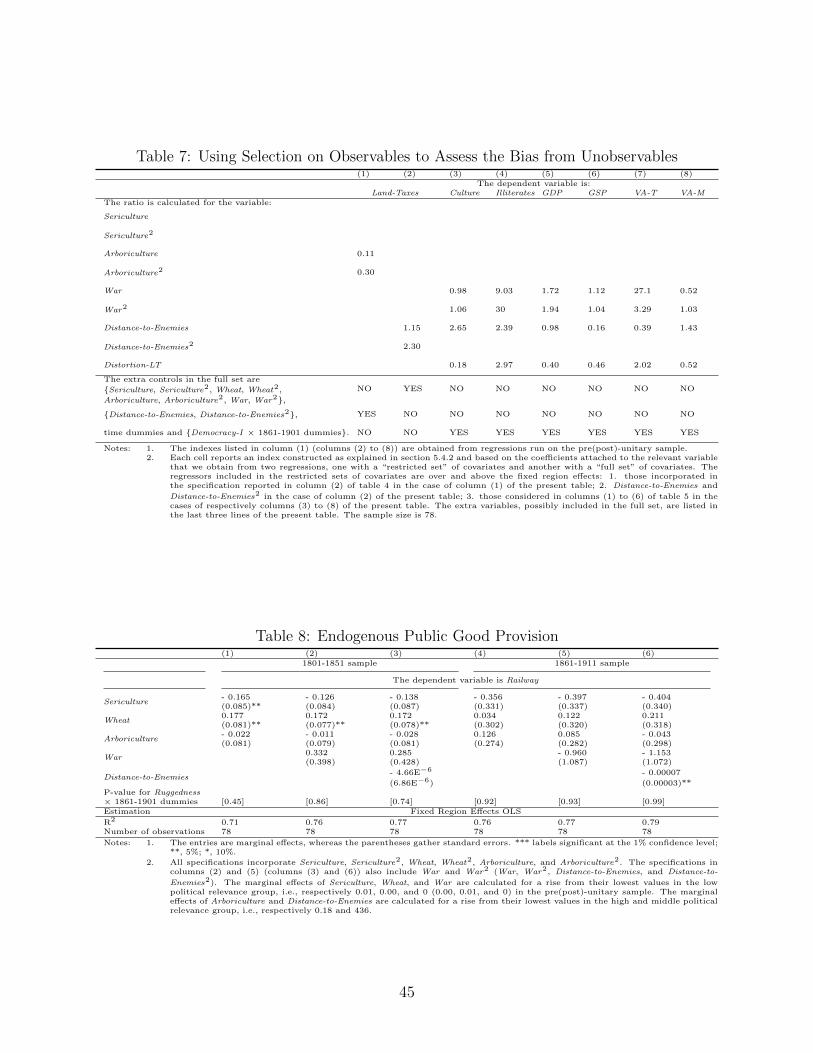
Table 7: Using Selection on Observables to Assess the Bias from Unobservables(1) (2) (3) (4) (5) (6) (7) (8)

The dependent variable is:Land-Taxes Culture Illiterates GDP GSP VA-T VA-M

The ratio is calculated for the variable:

Sericulture

Sericulture2

Arboriculture 0.11

Arboriculture2 0.30

War 0.98 9.03 1.72 1.12 27.1 0.52

War2 1.06 30 1.94 1.04 3.29 1.03

Distance-to-Enemies 1.15 2.65 2.39 0.98 0.16 0.39 1.43

Distance-to-Enemies2 2.30

Distortion-LT 0.18 2.97 0.40 0.46 2.02 0.52

The extra controls in the full set areNO YES NO NO NO NO NO NO{Sericulture, Sericulture2, Wheat, Wheat2,

Arboriculture, Arboriculture2, War, War2},

{Distance-to-Enemies, Distance-to-Enemies2}, YES NO NO NO NO NO NO NO

time dummies and {Democracy-I × 1861-1901 dummies}. NO NO YES YES YES YES YES YES

Notes: 1. The indexes listed in column (1) (columns (2) to (8)) are obtained from regressions run on the pre(post)-unitary sample.2. Each cell reports an index constructed as explained in section 5.4.2 and based on the coefficients attached to the relevant variable

that we obtain from two regressions, one with a “restricted set” of covariates and another with a “full set” of covariates. Theregressors included in the restricted sets of covariates are over and above the fixed region effects: 1. those incorporated inthe specification reported in column (2) of table 4 in the case of column (1) of the present table; 2. Distance-to-Enemies and

Distance-to-Enemies2 in the case of column (2) of the present table; 3. those considered in columns (1) to (6) of table 5 in thecases of respectively columns (3) to (8) of the present table. The extra variables, possibly included in the full set, are listed inthe last three lines of the present table. The sample size is 78.

Table 8: Endogenous Public Good Provision(1) (2) (3) (4) (5) (6)

1801-1851 sample 1861-1911 sample

The dependent variable is Railway

Sericulture- 0.165 - 0.126 - 0.138 - 0.356 - 0.397 - 0.404(0.085)** (0.084) (0.087) (0.331) (0.337) (0.340)

Wheat0.177 0.172 0.172 0.034 0.122 0.211(0.081)** (0.077)** (0.078)** (0.302) (0.320) (0.318)

Arboriculture- 0.022 - 0.011 - 0.028 0.126 0.085 - 0.043(0.081) (0.079) (0.081) (0.274) (0.282) (0.298)

War0.332 0.285 - 0.960 - 1.153(0.398) (0.428) (1.087) (1.072)

Distance-to-Enemies- 4.66E−6 - 0.00007

(6.86E−6) (0.00003)**P-value for Ruggedness× 1861-1901 dummies [0.45] [0.86] [0.74] [0.92] [0.93] [0.99]Estimation Fixed Region Effects OLS

R2 0.71 0.76 0.77 0.76 0.77 0.79Number of observations 78 78 78 78 78 78

Notes: 1. The entries are marginal effects, whereas the parentheses gather standard errors. *** labels significant at the 1% confidence level;**, 5%; *, 10%.

2. All specifications incorporate Sericulture, Sericulture2, Wheat, Wheat2, Arboriculture, and Arboriculture2. The specifications incolumns (2) and (5) (columns (3) and (6)) also include War and War2 (War, War2, Distance-to-Enemies, and Distance-to-

Enemies2). The marginal effects of Sericulture, Wheat, and War are calculated for a rise from their lowest values in the lowpolitical relevance group, i.e., respectively 0.01, 0.00, and 0 (0.00, 0.01, and 0) in the pre(post)-unitary sample. The marginaleffects of Arboriculture and Distance-to-Enemies are calculated for a rise from their lowest values in the high and middle politicalrelevance group, i.e., respectively 0.18 and 436.

45

APPENDIX (FOR ONLINE PUBLICATION)

I Establishing the Exogeneity of War

Next, we explain why War should be correctly considered exogenous.

Austro-Sardinian War

As soon as the revolutionaries expelled the Austrians from Milan in March 1848, the “Italianpopulation enthusiastically supported [Charles Albert’s] intervention” [Paoletti 2008, p. 96] sincethey knew that the Austrian army “could not get reinforcements [. . . ] because of the revolutionin Vienna” [Paoletti 2008, p. 96]. Mainly driven by the threat of internal unrests, Charles Albertthen “moved his troops into Lombardy” [Killinger 2002, p. 107]. Yet, the Habsburgs soon tamedthe turmoils and then defeated both the Savoys and their allies (Killinger, 2002). The truce wassigned in August 1848. All in all, none of the pre-unitary elites shaped the fate of this conflict.

Roman Republic War

Even if Pope Pius IX had granted his own constitution on February 14 1848, the liberals expelledhim in the aftermath of the truce the Kingdom of Sardinia reached with Austria and declared theRoman Republic in November 1848. This decision ignited the reactions of both the conservativeelite and the Catholic powers who sought to restore the Pope’s rule. In particular, “in a politicallycalculated attempt to win support of French Catholics, Louis Napoleon ordered his armies to restorethe Pope to power” [Killinger 2002, p. 109]. Meanwhile, Austria defeated again the Kingdom ofSardinia in Novara on March 23 1849, reinstating its power over Italy. In June 1849 a French armyinvaded the Papal State and defeated the “weak and ill-equipped [Roman Republican army]” [Riall2009, p. 23]. Again, none of the pre-unitary elites shaped the fate of this conflict.

Neapolitan and Italian-Roman Wars

In the aftermath of the 1848 unrests, the Bourbons “concentrated all [their effort] on domesticaffairs. [The] army was now intended to be more of a large, well-armed constabulary force” [Paoletti2008, p. 102]. After the royal forces crushed a revolt in Palermo, “Francesco Crispi, one of therevolutionaries, urged Garibaldi to intervene” [Paoletti 2008, p. 110] sure that the Bourbons couldbe overturned. Garibaldi assembled a group of volunteers, who departed from Genoa and reachedSicily in May 1860. Their arrival ignited a large scale revolt to which the Bourbons did notreact because scared by “an interposition by US, French, and British” [Paoletti 2008, p. 110].Garibaldi’s swift conquest of Sicily worried the European powers and the Kingdom of Sardinia“that the guerrilla leader might move on Naples, Rome, and Venice” [Killinger 2002, p. 116].Garibaldi’s conquest of Naples confirmed these suspects and forced Victor Emanuel II to try tostop him before he could put the independence at jeopardy (Paoletti, 2008). With the Frenchapproval, the Kingdom of Sardinia’s forces moved into the Papal State in September 1860 firingup the Italian-Roman War. The conflict ended a few months later with the Kingdom of Sardinia’sconquest of Marche and Umbria and the meeting between Garibaldi and Victor Emanuel II, whowas then proclaimed King of Italy (Killinger, 2002). All in all, both conflicts were guided by theexpansionist decisions of the Kingdom of Sardinia, France, and England and only barely affectedby the—lack of—adequate reactions by both the Kingdom of Two Sicilies and the Papal State.

Seven Weeks War

“In 1866, Prusso-Austrian competition for supremacy in Germany reached its zenith. Prussianchancellor Otto von Bismarck forced Austria to declare war on Prussia. [In] Bismarck’s opinion[. . . ], it was better to have Italy as an ally, because it prevented Austria from concentrating its

46

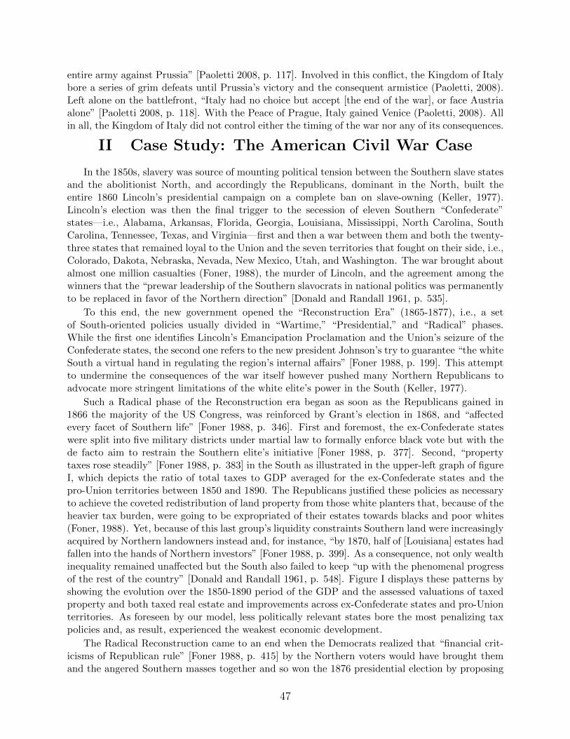
entire army against Prussia” [Paoletti 2008, p. 117]. Involved in this conflict, the Kingdom of Italybore a series of grim defeats until Prussia’s victory and the consequent armistice (Paoletti, 2008).Left alone on the battlefront, “Italy had no choice but accept [the end of the war], or face Austriaalone” [Paoletti 2008, p. 118]. With the Peace of Prague, Italy gained Venice (Paoletti, 2008). Allin all, the Kingdom of Italy did not control either the timing of the war nor any of its consequences.

II Case Study: The American Civil War Case

In the 1850s, slavery was source of mounting political tension between the Southern slave statesand the abolitionist North, and accordingly the Republicans, dominant in the North, built theentire 1860 Lincoln’s presidential campaign on a complete ban on slave-owning (Keller, 1977).Lincoln’s election was then the final trigger to the secession of eleven Southern “Confederate”states—i.e., Alabama, Arkansas, Florida, Georgia, Louisiana, Mississippi, North Carolina, SouthCarolina, Tennessee, Texas, and Virginia—first and then a war between them and both the twenty-three states that remained loyal to the Union and the seven territories that fought on their side, i.e.,Colorado, Dakota, Nebraska, Nevada, New Mexico, Utah, and Washington. The war brought aboutalmost one million casualties (Foner, 1988), the murder of Lincoln, and the agreement among thewinners that the “prewar leadership of the Southern slavocrats in national politics was permanentlyto be replaced in favor of the Northern direction” [Donald and Randall 1961, p. 535].

To this end, the new government opened the “Reconstruction Era” (1865-1877), i.e., a setof South-oriented policies usually divided in “Wartime,” “Presidential,” and “Radical” phases.While the first one identifies Lincoln’s Emancipation Proclamation and the Union’s seizure of theConfederate states, the second one refers to the new president Johnson’s try to guarantee “the whiteSouth a virtual hand in regulating the region’s internal affairs” [Foner 1988, p. 199]. This attemptto undermine the consequences of the war itself however pushed many Northern Republicans toadvocate more stringent limitations of the white elite’s power in the South (Keller, 1977).

Such a Radical phase of the Reconstruction era began as soon as the Republicans gained in1866 the majority of the US Congress, was reinforced by Grant’s election in 1868, and “affectedevery facet of Southern life” [Foner 1988, p. 346]. First and foremost, the ex-Confederate stateswere split into five military districts under martial law to formally enforce black vote but with thede facto aim to restrain the Southern elite’s initiative [Foner 1988, p. 377]. Second, “propertytaxes rose steadily” [Foner 1988, p. 383] in the South as illustrated in the upper-left graph of figureI, which depicts the ratio of total taxes to GDP averaged for the ex-Confederate states and thepro-Union territories between 1850 and 1890. The Republicans justified these policies as necessaryto achieve the coveted redistribution of land property from those white planters that, because of theheavier tax burden, were going to be expropriated of their estates towards blacks and poor whites(Foner, 1988). Yet, because of this last group’s liquidity constraints Southern land were increasinglyacquired by Northern landowners instead and, for instance, “by 1870, half of [Louisiana] estates hadfallen into the hands of Northern investors” [Foner 1988, p. 399]. As a consequence, not only wealthinequality remained unaffected but the South also failed to keep “up with the phenomenal progressof the rest of the country” [Donald and Randall 1961, p. 548]. Figure I displays these patterns byshowing the evolution over the 1850-1890 period of the GDP and the assessed valuations of taxedproperty and both taxed real estate and improvements across ex-Confederate states and pro-Unionterritories. As foreseen by our model, less politically relevant states bore the most penalizing taxpolicies and, as result, experienced the weakest economic development.

The Radical Reconstruction came to an end when the Democrats realized that “financial crit-icisms of Republican rule” [Foner 1988, p. 415] by the Northern voters would have brought themand the angered Southern masses together and so won the 1876 presidential election by proposing

47

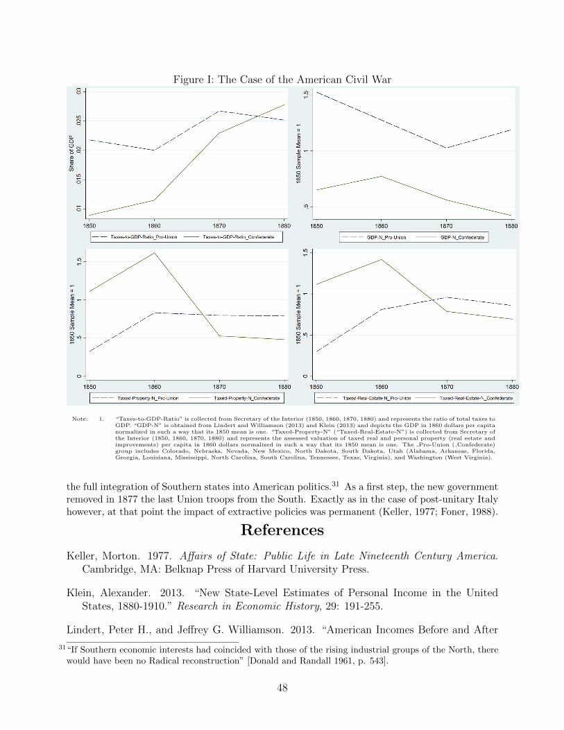
Figure I: The Case of the American Civil War

Note: 1. “Taxes-to-GDP-Ratio” is collected from Secretary of the Interior (1850, 1860, 1870, 1880) and represents the ratio of total taxes toGDP. “GDP-N” is obtained from Lindert and Williamson (2013) and Klein (2013) and depicts the GDP in 1860 dollars per capitanormalized in such a way that its 1850 mean is one. “Taxed-Property-N” (“Taxed-Real-Estate-N”) is collected from Secretary ofthe Interior (1850, 1860, 1870, 1880) and represents the assessed valuation of taxed real and personal property (real estate andimprovements) per capita in 1860 dollars normalized in such a way that its 1850 mean is one. The Pro-Union ( Confederate)group includes Colorado, Nebraska, Nevada, New Mexico, North Dakota, South Dakota, Utah (Alabama, Arkansas, Florida,Georgia, Louisiana, Mississippi, North Carolina, South Carolina, Tennessee, Texas, Virginia), and Washington (West Virginia).

the full integration of Southern states into American politics.31 As a first step, the new governmentremoved in 1877 the last Union troops from the South. Exactly as in the case of post-unitary Italyhowever, at that point the impact of extractive policies was permanent (Keller, 1977; Foner, 1988).

References

Keller, Morton. 1977. Affairs of State: Public Life in Late Nineteenth Century America.Cambridge, MA: Belknap Press of Harvard University Press.

Klein, Alexander. 2013. “New State-Level Estimates of Personal Income in the UnitedStates, 1880-1910.” Research in Economic History, 29: 191-255.

Lindert, Peter H., and Jeffrey G. Williamson. 2013. “American Incomes Before and After

31“If Southern economic interests had coincided with those of the rising industrial groups of the North, therewould have been no Radical reconstruction” [Donald and Randall 1961, p. 543].

48

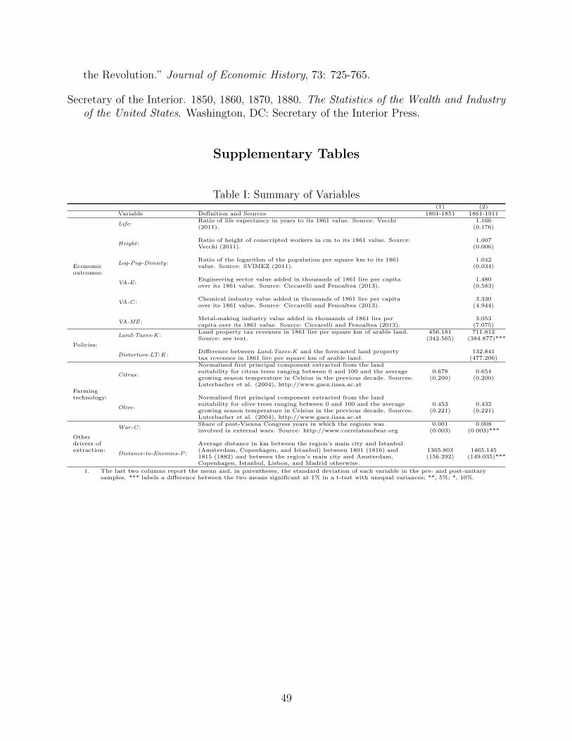
the Revolution.” Journal of Economic History, 73: 725-765.

Secretary of the Interior. 1850, 1860, 1870, 1880. The Statistics of the Wealth and Industryof the United States. Washington, DC: Secretary of the Interior Press.

Supplementary Tables

Table I: Summary of Variables(1) (2)

Variable Definition and Sources 1801-1851 1861-1911

Life:Ratio of life expectancy in years to its 1861 value. Source: Vecchi 1.166(2011). (0.176)

Height:Ratio of height of conscripted workers in cm to its 1861 value. Source: 1.007Vecchi (2011). (0.006)

Log-Pop-Density:Ratio of the logarithm of the population per square km to its 1861 1.042

Economic value. Source: SVIMEZ (2011). (0.034)outcomes:

VA-E :Engineering sector value added in thousands of 1861 lire per capita 1.480over its 1861 value. Source: Ciccarelli and Fenoaltea (2013). (0.583)

VA-C :Chemical industry value added in thousands of 1861 lire per capita 3.330over its 1861 value. Source: Ciccarelli and Fenoaltea (2013). (4.944)

VA-ME :Metal-making industry value added in thousands of 1861 lire per 3.053capita over its 1861 value. Source: Ciccarelli and Fenoaltea (2013). (7.075)

Land-Taxes-K :Land property tax revenues in 1861 lire per square km of arable land. 456.181 711.812Source: see text. (342.565) (384.877)***

Policies:

Distortion-LT-K :Difference between Land-Taxes-K and the forecasted land property 132.841tax revenues in 1861 lire per square km of arable land. (477.206)

Citrus:

Normalized first principal component extracted from the landsuitability for citrus trees ranging between 0 and 100 and the average 0.678 0.654growing season temperature in Celsius in the previous decade. Sources: (0.200) (0.200)Luterbacher et al. (2004), http://www.gaez.iiasa.ac.at

Farmingtechnology:

Olive:

Normalized first principal component extracted from the landsuitability for olive trees ranging between 0 and 100 and the average 0.453 0.432growing season temperature in Celsius in the previous decade. Sources: (0.221) (0.221)Luterbacher et al. (2004), http://www.gaez.iiasa.ac.at

War-C :Share of post-Vienna Congress years in which the regions was 0.001 0.008involved in external wars. Source: http://www.correlatesofwar.org (0.003) (0.003)***

Otherdrivers of

Distance-to-Enemies-P:

Average distance in km between the region’s main city and Istanbulextraction: (Amsterdam, Copenhagen, and Istanbul) between 1801 (1816) and 1365.803 1465.145

1815 (1882) and between the region’s main city and Amsterdam, (156.292) (149.035)***Copenhagen, Istanbul, Lisbon, and Madrid otherwise.

1. The last two columns report the mean and, in parentheses, the standard deviation of each variable in the pre- and post-unitarysamples. *** labels a difference between the two means significant at 1% in a t-test with unequal variances; **, 5%; *, 10%.

49

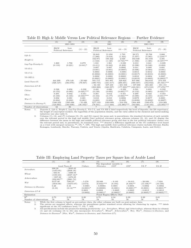
Table II: High & Middle Versus Low Political Relevance Regions — Further Evidence(1) (2) (3) (4) (5) (6) (7) (8) (9)

1801-1851 1861 1861-1911

H&M Low(1) - (2)

H&M Low(4) - (5)

H&M Low(7) - (8)

Political Relevance Political Relevance Political Relevance

Life-L:32.843 31.050 1.793 38.571 35.706 2.866(1.280) (3.018) (1.324) (5.357) (5.365) (1.218)**

Height-L:162.971 160.322 2.649 164.048 161.656 2.391(1.543) (1.129) (0.743)*** (1.590) (1.385) (0.337)***

Log-Pop-Density-L:1.869 1.790 0.079 1.931 1.961 - 0.030 2.013 2.041 - 0.029

(0.119) (0.221) (0.041)* (0.411) (0.343) (0.209) (0.398) (0.346) (0.084)

VA-E-L:0.007 0.007 0.0005 0.011 0.009 0.001

(0.001) (0.001) (0.0007) (0.006) (0.004) (0.001)

VA-C-L:0.0004 0.0006 - 0.0001 0.0015 0.0012 0.0003

(0.0002) (0.0003) (0.0001) (0.0017) (0.0010) (0.0003)

VA-ME-L:0.0002 0.0002 0.00001 0.0010 0.0004 0.0007

(0.0001) (0.0002) (0.0001) (0.0019) (0.0005) (0.0003)**

Land-Taxes-K :444.209 470.149 - 25.940 931.715 601.891 329.824 837.966 564.633 273.333

(326.127) (364.976) (78.947) (496.755) (441.617) (260.301) (369.507) (352.942) (81.921)***

Distortion-LT-K :- 94.120 507.439 - 601.558 - 167.690 483.460 - 651.151

(293.988) (340.597) (177.993)*** (403.581) (274.533) (77.276)***

Citrus:0.526 0.856 - 0.330 0.491 0.820 - 0.329 0.501 0.833 - 0.332

(0.133) (0.085) (0.025)*** (0.139) (0.093) (0.065)*** (0.132) (0.085) (0.025)***

Olive:0.291 0.642 - 0.351 0.261 0.612 - 0.351 0.269 0.622 - 0.353

(0.100) (0.165) (0.032)*** (0.104) (0.177) (0.082)*** (0.099) (0.165) (0.031)***

War-C :0.002 0.001 0.001 0.010 0.010 0.0002 0.0079 0.0077 0.0001

(0.004) (0.002) (0.001) (0.005) (0.002) (0.002) (0.0038) (0.0022) (0.0007)

Distance-to-Enemy-P:1340.222 1395.648 - 55.426 1277.333 1493.889 - 216.556 1364.406 1582.674 - 218.268(124.664) (183.938) (36.192)* (78.501) (111.630) (54.380)*** (94.026) (110.105) (23.393)***

Number of observations 42 36 7 6 42 36

Notes: 1. Deposits-L, Life-L, Height-L, Log-Pop-Density-L, VA-C-L, and VA-ME-L label respectively the level of deposits, the life expectancy,the height of conscripted workers, the logarithm of the population density, and the value added in the chemical and metal-makingindustries (see also table I).

2. Columns (1), (4), and (7) (columns (2), (5), and (8)) report the mean and, in parentheses, the standard deviation of each variableover the relevant period in the high and middle (low) political relevance group, whereas columns (3), (6), and (9) display thedifference between the mean in the high and middle political relevance group and that in the low political relevance cluster overthe relevant period and, in parentheses, its standard error. *** denotes a difference significant at the 1% confidence level basedon a t-test with unequal variances; **, 5%; *, 10%. The high and middle (low) political relevance cluster includes Abruzzi, EmiliaRomagna, Lombardy, Marche, Tuscany, Umbria, and Veneto (Apulia, Basilicata, Calabria, Campania, Lazio, and Sicily).

Table III: Employing Land Property Taxes per Square km of Arable Land(1) (2) (3) (4) (5) (6) (7) (8)

The dependent variable is:Land-Taxes-K Culture Illiterates GDP GSP VA-T VA-M

Sericulture698.28 - 2043.43(1453.05) (2936.18)

Wheat- 693.91 - 3388.59(1355.63) (2027.16)*

Arboriculture- 1937.00 - 2476.05(932.69)** (3961.74)

War6137.48 7283.07 - 5.578 22.949 - 9.165 - 18.613 - 29.936 - 7.024(3916.00) (16273.97) (3.674) (6.032)*** (9.194) (8.330)** (13.168)** (10.539)

Distance-to-Enemies0.26 0.44 - 0.0001 - 0.00004 0.0001 - 0.0004 - 0.0002 - 0.0002(0.16) (0.14)*** (0.0001)* (0.00005) (0.0001) (0.0001)** (0.0001) (0.0001)**

Distortion-LT-K0.0001 0.0002 - 0.0005 - 0.0003 - 0.0013 - 0.0012(0.0002) (0.0001)* (0.0003)* (0.0003) (0.0005)** (0.0003)***

Estimation Fixed Region Effects OLS

R2 0.73 0.24 0.20 0.75 0.34 0.30 0.29 0.61Number of observations 78 78 78 78 78 78 78 78

Notes: 1. While the first column is based on pre-unitary data, the other columns are built on post-unitary data.2. The entries are marginal effects, whereas the parentheses gather standard errors allowing for clustering by region. *** labels

significant at the 1% confidence level; **, 5%; *, 10%.3. All specifications include the proxies for farming productivity—i.e., Sericulture, Wheat, and Arboriculture, whereas those in columns

(1) and (2) (columns (3) to (8)) also incorporate Sericulture2, Wheat2, Arboriculture2, War, War2, Distance-to-Enemies, and

Distance-to-Enemies2 (War, War2, Distance-to-Enemies, and Distortion-LT).

50

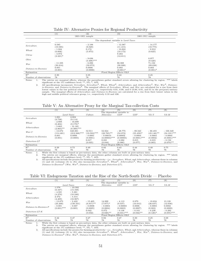
Table IV: Alternative Proxies for Regional Productivity(1) (2) (3) (4)

1801-1851 sample 1861-1911 sample

The dependent variable is Land-Taxes

Sericulture0.585 - 2.188 - 12.387 - 14.177(10.585) (8.029) (11.415) (10.775)

Wheat- 1.924 0.172 - 10.824 - 9.912(6.608) (5.973) (10.172) (9.825)

Citrus- 3.972 9.484(2.221)* (12.011)

Olive- 9.636 0.977(3.406)*** (9.420)

War- 11.335 - 6.096 86.308 71.156(30.214) (32.073) (90.928) (89.638)

Distance-to-Enemies0.001 0.0006 0.002 0.002(0.001) (0.0008) (0.001)* (0.001)*

Estimation Fixed Region Effects OLS

R2 0.30 0.35 0.44 0.45Number of observations 78 78 78 78

Notes: 1. The entries are marginal effects, whereas the parentheses gather standard errors allowing for clustering by region. *** labelssignificant at the 1% confidence level; **, 5%; *, 10%.

2. All specifications incorporate Sericulture, Sericulture2, Wheat, Wheat2, Arboriculture, and Arboriculture2, War, War2, Distance-to-Enemies, and Distance-to-Enemies2. The marginal effects of Sericulture, Wheat, and War are calculated for a rise from theirlowest values in the low political relevance group, i.e., respectively 0.01, 0.00, and 0 (0.00, 0.01, and 0) in the pre(post)-unitarysample. The marginal effects of Arboriculture and Distance-to-Enemies are calculated for a rise from their lowest values in thehigh and middle political relevance group, i.e., respectively 0.18 and 436.

Table V: An Alternative Proxy for the Marginal Tax-collection Costs(1) (2) (3) (4) (5) (6) (7) (8)

The dependent variable is:Land-Taxes Culture Illiterates GDP GSP VA-T VA-M

Sericulture1.001 2.004(9.738) (9.114)

Wheat- 2.808 - 16.690(6.204) (9.179)*

Arboriculture- 5.663 - 31.181(2.863)** (8.389)***

War-C- 13.672 648.881 52.911 52.824 - 28.775 - 89.343 - 86.455 - 106.349(114.461) (212.566)*** (19.593)*** (22.765)** (54.072) (55.459)* (45.146)** (34.101)***

Distance-to-Enemies0.001 0.0006 - 0.0001 - 0.00010 0.00002 - 0.0004 - 0.0004 - 0.0004(0.001) (0.0005) (0.0001) (0.00003)*** (0.00005) (0.0001)*** (0.0002) (0.0001)***

Distortion-LT0.017 0.021 - 0.082 0.015 - 0.019 - 0.156(0.025) (0.044) (0.086) (0.077) (0.065) (0.070)**

Estimation Fixed Region Effects OLS

R2 0.29 0.73 0.49 0.82 0.43 0.44 0.48 0.75Number of observations 78 78 78 78 78 78 78 78

Notes: 1. While the first column is based on pre-unitary data, the other columns are built on post-unitary data.2. The entries are marginal effects, whereas the parentheses gather standard errors allowing for clustering by region. *** labels

significant at the 1% confidence level; **, 5%; *, 10%.3. All specifications include the proxies for farming productivity—i.e., Sericulture, Wheat, and Arboriculture, whereas those in columns

(1) and (2) (columns (3) to (8)) also incorporate Sericulture2, Wheat2, Arboriculture2, War, War2, Distance-to-Enemies, and

Distance-to-Enemies2 (War, War2, Distance-to-Enemies, and Distortion-LT).

Table VI: Endogenous Taxation and the Rise of the North-South Divide — Placebo(1) (2) (3) (4) (5) (6) (7) (8)

The dependent variable is:Land-Taxes Culture Illiterates GDP GSP VA-T VA-M

Sericulture1.578 - 19.392(6.447) (15.168)

Wheat- 4.591 - 5.261(4.270) (16.246)

Arboriculture2.472 - 5.414(4.409) (16.967)

War- 13.073 - 2.422 - 15.405 14.999 - 4.113 0.979 - 19.834 13.120(25.268) (130.331) (6.917)** (7.977)* (9.537) (10.012) (26.637) (12.636)

Distance-to-Enemies-P- 0.001 - 0.007 - 0.0008 - 0.0004 - 0.00003 0.0006 - 0.0003 0.0002(0.001)*** (0.005) (0.0005) (0.0004) (0.0003) (0.0007) (0.002) (0.0009)

Distortion-LT-K0.042 0.072 - 0.138 - 0.101 - 0.238 - 0.282(0.032) (0.026)** (0.041)*** (0.042)** (0.120)* (0.055)***

Estimation Fixed Region Effects OLS

R2 0.42 0.47 0.27 0.82 0.47 0.30 0.25 0.68Number of observations 78 78 78 78 78 78 78 78

Notes: 1. While the first column is based on pre-unitary data, the other columns are built on post-unitary data.2. The entries are marginal effects, whereas the parentheses gather standard errors allowing for clustering by region. *** labels

significant at the 1% confidence level; **, 5%; *, 10%.3. All specifications include the proxies for farming productivity—i.e., Sericulture, Wheat, and Arboriculture, whereas those in columns

(1) and (2) (columns (3) to (8)) also incorporate Sericulture2, Wheat2, Arboriculture2, War, War2, Distance-to-Enemies, and

Distance-to-Enemies2 (War, War2, Distance-to-Enemies, and Distortion-LT).

51

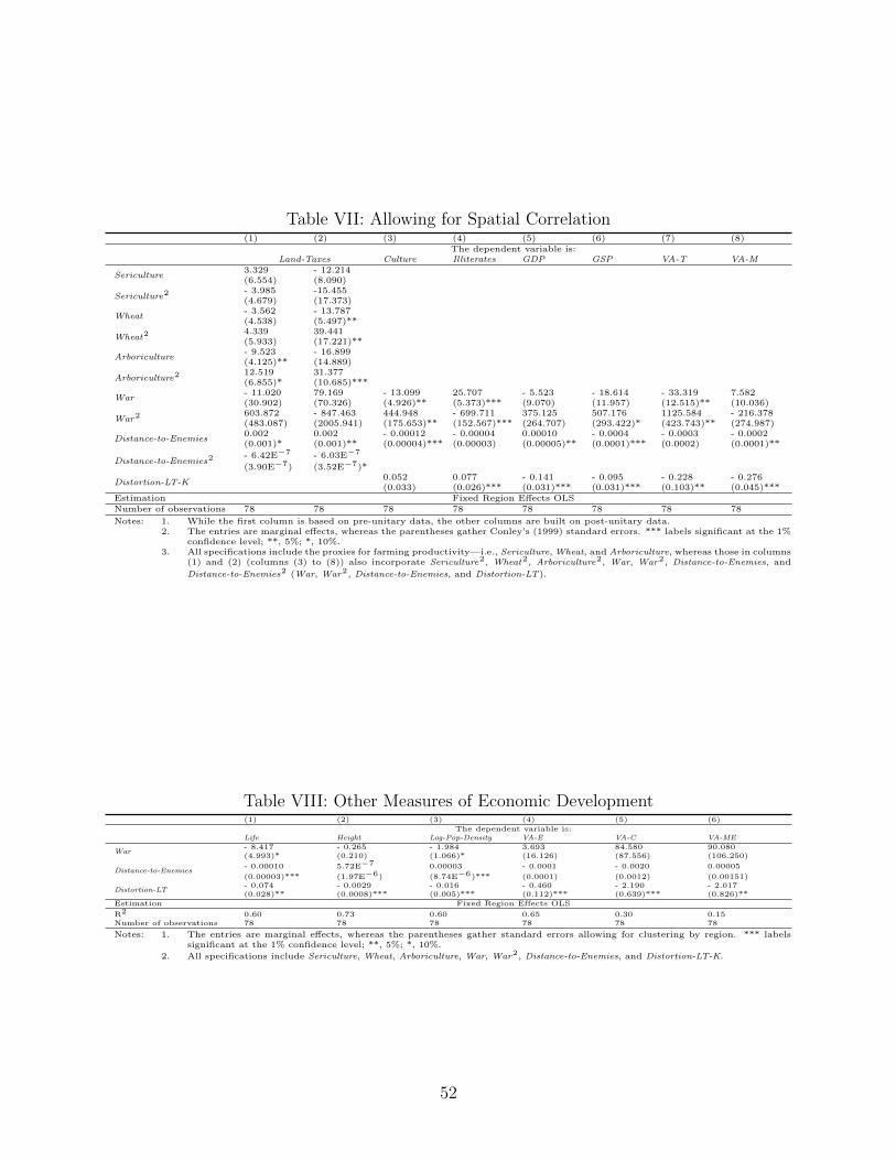
Table VII: Allowing for Spatial Correlation(1) (2) (3) (4) (5) (6) (7) (8)

The dependent variable is:Land-Taxes Culture Illiterates GDP GSP VA-T VA-M

Sericulture3.329 - 12.214(6.554) (8.090)

Sericulture2- 3.985 -15.455(4.679) (17.373)

Wheat- 3.562 - 13.787(4.538) (5.497)**

Wheat24.339 39.441(5.933) (17.221)**

Arboriculture- 9.523 - 16.899(4.125)** (14.889)

Arboriculture212.519 31.377(6.855)* (10.685)***

War- 11.020 79.169 - 13.099 25.707 - 5.523 - 18.614 - 33.319 7.582(30.902) (70.326) (4.926)** (5.373)*** (9.070) (11.957) (12.515)** (10.036)

War2603.872 - 847.463 444.948 - 699.711 375.125 507.176 1125.584 - 216.378(483.087) (2005.941) (175.653)** (152.567)*** (264.707) (293.422)* (423.743)** (274.987)

Distance-to-Enemies0.002 0.002 - 0.00012 - 0.00004 0.00010 - 0.0004 - 0.0003 - 0.0002(0.001)* (0.001)** (0.00004)*** (0.00003) (0.00005)** (0.0001)*** (0.0002) (0.0001)**

Distance-to-Enemies2- 6.42E−7 - 6.03E−7

(3.90E−7) (3.52E−7)*

Distortion-LT-K0.052 0.077 - 0.141 - 0.095 - 0.228 - 0.276(0.033) (0.026)*** (0.031)*** (0.031)*** (0.103)** (0.045)***

Estimation Fixed Region Effects OLSNumber of observations 78 78 78 78 78 78 78 78

Notes: 1. While the first column is based on pre-unitary data, the other columns are built on post-unitary data.2. The entries are marginal effects, whereas the parentheses gather Conley’s (1999) standard errors. *** labels significant at the 1%

confidence level; **, 5%; *, 10%.3. All specifications include the proxies for farming productivity—i.e., Sericulture, Wheat, and Arboriculture, whereas those in columns

(1) and (2) (columns (3) to (8)) also incorporate Sericulture2, Wheat2, Arboriculture2, War, War2, Distance-to-Enemies, and

Distance-to-Enemies2 (War, War2, Distance-to-Enemies, and Distortion-LT).

Table VIII: Other Measures of Economic Development(1) (2) (3) (4) (5) (6)

The dependent variable is:Life Height Log-Pop-Density VA-E VA-C VA-ME

War- 8.417 - 0.265 - 1.984 3.693 84.580 90.080(4.993)* (0.210) (1.066)* (16.126) (87.556) (106.250)

Distance-to-Enemies- 0.00010 5.72E−7 0.00003 - 0.0001 - 0.0020 0.00005

(0.00003)*** (1.97E−6) (8.74E−6)*** (0.0001) (0.0012) (0.00151)

Distortion-LT- 0.074 - 0.0029 - 0.016 - 0.460 - 2.190 - 2.017(0.028)** (0.0008)*** (0.005)*** (0.112)*** (0.639)*** (0.826)**

Estimation Fixed Region Effects OLS

R2 0.60 0.73 0.60 0.65 0.30 0.15Number of observations 78 78 78 78 78 78

Notes: 1. The entries are marginal effects, whereas the parentheses gather standard errors allowing for clustering by region. *** labelssignificant at the 1% confidence level; **, 5%; *, 10%.

2. All specifications include Sericulture, Wheat, Arboriculture, War, War2, Distance-to-Enemies, and Distortion-LT-K.

52