Extending Hirshfeld-I to bulk and periodic materials

D. E. P. Vanpoucke,1, 2 P. Bultinck,2 and I. Van Driessche1

1SCRiPTS group, Dept. Inorganic and Physical Chemistry,Ghent University, Krijgslaan 281 - S3, 9000 Gent, Belgium

2Ghent Quantum Chemistry Group, Dept. Inorganic and Physical Chemistry,Ghent University, Krijgslaan 281 - S3, 9000 Gent, Belgium

(Dated: July 13, 2012)

In this work, a method is described to extend the iterative Hirshfeld-I method, generally used formolecules, to periodic systems. The implementation makes use of precalculated pseudo-potentialbased electron density distributions, and it is shown that high quality results are obtained for bothmolecules and solids, such as ceria, diamond, and graphite. The use of grids containing (precal-culated) electron densities makes the implementation independent of the solid state or quantumchemical code used for studying the system. The extension described here allows for easy calcu-lation of atomic charges and charge transfer in periodic and bulk systems. The conceptual issueof obtaining reference densities for anions is discussed and the delocalization problem for anionicreference densities originating from the use of a plane wave basis set is identified and handled.

PACS numbers:

I. INTRODUCTION

One of the most successful concepts in chemistry isthat of “atoms in molecules” (AIM). It states that theproperties of a molecule can be seen as simple sums ofthe properties of its constituent atoms. An impressiveamount of insights has been obtained from such a view-point, although a precise definition of an AIM remainselusive.1–3 All AIM methods have the common purposeof trying to improve our understanding of chemicalconcepts such as molecular similarity and transferabilitybetween molecules.4 Since the concept of AIM is basi-cally about how one should divide the electrons, morespecifically the electron density distribution (EDD)ρ(r) in the molecule between the different “atoms”,this leads to two obvious categories of approaches inwhich most of the methods used for defining AIM canbe divided. The first category of approaches is basedon the wave-function/states of the system, and mostof the work is performed in the Hilbert space of thebasis functions used. One of the most famous exampleshere is the Mulliken approach.5,6 The second categoryof approaches is based on the division of the EDD as itexists in real-space. In these real-space approaches themolecule is split into atomic basins, that can overlapsuch as in the Hirshfeld7 and derived methods,8–12 orthat are non-overlapping such as in Bader’s approach.13

The concept of AIM is strongly linked to the conceptof transferability. Because both are central in chemistry,and chemists mainly focus on molecules, they are mostlyused for molecules.14,15 There is, however, no reasonwhy these concepts should not be applicable for periodicsystems such as bulk materials. Even more, if theseconcepts are truly valid, they should hold equally wellfor solids as for molecules, and should provide additionalinsight in the chemical properties of defects, such asdopants, interfaces and adsorption of molecules onsurfaces.

To this date we are aware of few implementationsfor periodic systems of the Hirshfeld and Hirshfeld-Iapproach, but their number is steadily rising. MartınPendas et al.16 investigated Hirshfeld surfaces as ap-proximations for interatomic surfaces for LiF and CS2

crystals. The Cut3D plugin of the ABINIT codecan be used to calculate Hirshfeld charges,17–20 andrecently Leenaerts et al. implemented a “subsystem”based Hirshfeld-I method to study graphane, graphenefluoride and paramagnetic adsorbates on graphene.21–23Similarly, Spackman and collaborators presentedsubsystem-based Hirshfeld surfaces for molecularsolids and implemented this in their Crystal-Explorercode.24–28 In a recent publication Watanabe et al.29presented Hirshfeld results for metal–organic frameworksusing the DDEC-code of Manz and Sholl.12 The samecode was probably also used in the investigation ofcharge injection in graphene layers by Rogers and Liu.30These authors present Hirshfeld-I charges, though theydo not mention explicitly how these were obtained. Inthis DDEC code the function which is minimized is alinear combination of the function minimized in theHirshfeld-I method, the one minimized in the iterativestockholder approach, and an additional term enforcingthe constraint that all electron density is accountedfor.8–12 At the time of writing Verstraelen et al. showedthat an excellent reproduction of the electrostaticpotential (ESP) in silicates is possible using Hirshfeld-Icharges.31

In this work, we have implemented an extension of theiterative Hirshfeld-I approach9 to periodic systems, as amodule in our HIVE-code.32 The implementation makesuse of grid stored EDDs, which can easily be generatedby standard solid state and quantum chemical codes.

In Sec. II a short review of the parameters used in thesolid state and quantum chemical codes is given. After-wards the basic theory behind the Hirshfeld-I methodis presented and extended to periodic systems. In

2

addition, the spatial integration grid, pseudo-potentialsand stored EDDs are discussed in view of the Hirshfeld-Imethod for periodic systems. In Sec. III the influenceof the different grids on the accuracy is discussed. Wealso identify a delocalization problem in the radialEDDs which originates from the plane wave approachand periodic boundary conditions (PBC) used in thesolid state code. This delocalization problem showsan inherent conceptual problem exists when referencedensities need to be generated for anions. We shortlydiscuss this conceptual issue in Sec. III C and indicateif and how it is handled in other implementations.We present two effective solutions ourselves, and showhow these improve the obtained results. In Sec. III Dthe influence of the inclusion of core electrons in thereference densities is presented. As a last point, theatomic charges in some simple periodic systems arecalculated, showing that the algorithm works correctly.Finally, in Sec. IV some conclusions are given.

II. METHODS

A. Atomic and molecular calculations

Hirshfeld-I calculations require EDDs as input. Thesecan be obtained from electronic structure calculationsusing standard solid state or quantum chemical codes.In this work we have chosen to perform these calcu-lations within the DFT framework using the projectoraugmented wave (PAW) approach for the core-valenceinteraction and the local density approximation (LDA)for the exchange-correlation functional as implementedin the VASP code.33,34 The kinetic energy cut-off is setat 500 eV and the k-point set is reduced to the Γ-point formolecular and atomic calculations. For the bulk materi-als sufficiently converged k-point sets were used. To opti-mize the geometry of the molecules and periodic materi-als a conjugate gradient algorithm is applied. For molec-ular calculations only the atom positions are optimized,for bulk materials the cell parameters are optimized si-multaneously. All molecules are placed in periodic cellsof 20.0×21.0×20.5A3, which provide a sufficiently largevacuum region between periodic copies of the molecules,to prevent interaction.

Hirshfeld-I data computed using the approach detailedin the present study, are compared to those obtained us-ing more common molecular calculations of AIM prop-erties. For the set of 168 neutral molecules previouslystudied by Bultinck et al.,9,35 geometry optimizationand Hirshfeld-I charge calculations are performed at theLocal Spin Density Approximation36,37 level with theSlater exchange functional38 and the VWN5 correlationfunctional39 as implemented in Gaussian-03.40 Numericalintegrations are carried out using Becke’s integration gridwith 170 angular points in the Lebedev-Laikov grid.41,42The Hirshfeld-I charges are considered converged if the

largest change in charge of any atom is below 0.0005e.

B. Hirshfeld methods

The basic idea behind the Hirshfeld method,7 alsoknown as the stockholder method, is that the AIM sharethe electron density in each point of space. This meansthat the AIM EDD becomes a weighted partition of themolecular EDD. Formally this can be written as:

ρmol(r) =∑A

ρAIMA (r)

ρAIMA (r) = wH

A (r)ρmol(r) ∀r (1)

with∑A

wHA (r) ≡ 1,

with ρmol(r) and ρAIMA (r) the EDDs for the molecule and

the AIM. All sums are taken over the entire set of AIM,and wH

A (r) is the Hirshfeld weight function for atom A.From these equations the Hirshfeld weight can be writtenas:

wHA (r) =

ρAIMA (r)∑

B ρAIMB (r)

. (2)

Since the ρAIM (r) are the EDDs sought, they cannot beused as input. The Hirshfeld method circumvents thisproblem by using spherically averaged reference stateatomic EDDs ρ◦X(r). In the original paper by Hirsh-feld the neutral atomic ground state is used as referencestate.7 When summing these isolated atomic EDDs overall AIM, one gets the so-called ‘promolecular ’ EDD in-stead of the actual molecular EDD:

ρpromol(r) =∑B

ρ◦B(r). (3)

It is then assumed that the difference between this pro-molecular EDD and the actual molecular EDD has onlylittle influence on the Hirshfeld weight wH

A (r). As a resultone can write the EDD of an AIM A as:

ρAIMA (r) =

ρ◦A(n◦A, r)ρpromol(r)

ρmol(r), (4)

where the population of the atom A is given by n◦A. In theoriginal Hirshfeld approach, neutral atoms were used asreference. This, however, has been identified by severalauthors to be a major weakness of the method as chang-ing the choice of the promolecular atom charges can havea highly significant effect on the resulting AIM2,3,9,43,44

From eq.(4) it is easy to understand that the result-ing ρAIM

A (r) will tend to be as similar to ρ◦A(n◦A, r) aspossible1,9,45, explaining why the Hirshfeld populationsstrongly depend on the choice of reference atomic EDDs.Fortunately, this problem can be resolved by using theiterative Hirshfeld-I scheme.8,9 For each iteration i, theobtained ρAIM

A (r) are used to calculate the population

3

niA of each atom A. The (spherically symmetric) EDDρi

A(niA, r) of a free atom A with population ni

A is thenused as atomic EDD in wH

A (r). For each iteration thenew promolecular density ρi

promol(r) is obtained by sum-ming the density distributions ρi

A(niA, r) for all atoms of

the molecule. This setup is independent of the initialchoice of atomic EDDs and the convergence of the it-erative scheme is determined by the convergence of thepopulations of the AIM.46,47 Note that the first step inthis scheme usually corresponds to the standard Hirsh-feld method with n◦X = ZX . At this point it is impor-tant to note that the EDDs ρAIM

A (r) and ρiA(ni

A, r) willgenerally be different, despite having the same popula-tion. ρi

A(niA, r) is constructed as a spherically symmetric

EDD, whereas ρAIMA (r) is a weighted part of the molecu-

lar EDD. The resulting EDD will generally be not spher-ically symmetric but show protrusions along the direc-tions bonds are formed.

The extension of the Hirshfeld and Hirshfeld-I meth-ods from molecules to bulk and other periodic materialsis quite trivial from the formal perspective. The mainproblem is located in the fact that a bulk system is con-sidered to consist of an infinite number of “atoms in thesystem”(AIS). Calculating the atomic electron densitiesfor all AIS can, for a periodic system, be reduced to onlythe atoms in a single unit cell since all periodic copiesshould yield the same results.

In addition to this, also the summation limits inEqs. (2), (3) and (4) change. Where for molecules thesum over B is a finite sum over all AIM, it becomes aninfinite sum over all AIS. Because atomic EDDs drop ex-ponentially, the density contribution to the “prosystem”EDD ρprosys(r) =

∑AISB ρ◦B(n◦B , r) of atoms at larger

distances becomes negligible. This allows us to truncatethe infinite sum to include only the atoms within a cer-tain ‘sphere of influence’ (SoI), i.e. all atoms of whichthe contribution to the prosystem EDD is not negligible.Within the iterative Hirshfeld-I scheme we then get:

wH,iA (r) =

ρi−1A (ni−1

A , r)∑SoIB ρi−1

B (ni−1B , r)

∀A ε unit cell (5)

where

SoI∑A

wH,iA (r) ≤

AIS∑A

wH,iA (r) ≡ 1 ∀r, (6)

with i indicating the iteration step, and ρiA(ni

A, r) theatomic EDD for an atom A with a population ni

A givenby

niA =

∫wH,i

A (r)ρsystem(r)dr, (7)

where ρsystem(r) is the EDD of the periodic system.

C. Spatial integration of the population

In chemistry, due to the exponential decay of the elec-tron density of atoms and molecules, and due to the sharpcusps present in EDDs at the atomic nuclei, atom cen-tered grids are widely and successfully used. This makesthem ideally suited for integrations such as given in Eq.(7). The multicenter integration scheme proposed byBecke splits up the full space integration into a set ofoverlapping atom centered spherical integrations.41 Tosolve the problem of double counting in the overlappingregions a weight hA(r) is given to each point in space forevery atom A in the system, such that

AIS∑A

hA(r) ≡ 1 ∀r. (8)

This weight function indicates how much a point ‘be-longs’ to a certain atom A. The weight function can bebinary, when the space is split up in Voronoi or WignerSeitz cells,48,49 or smoothly varying, as is the case in theBecke scheme.41 As a result, an integrand F (r) can bedecomposed as F (r) =

∑AISA hA(r)FA(r) and the full

integration becomes

I =∫F (r)dr =

AIS∑A

∫hA(r)FA(r)dr, (9)

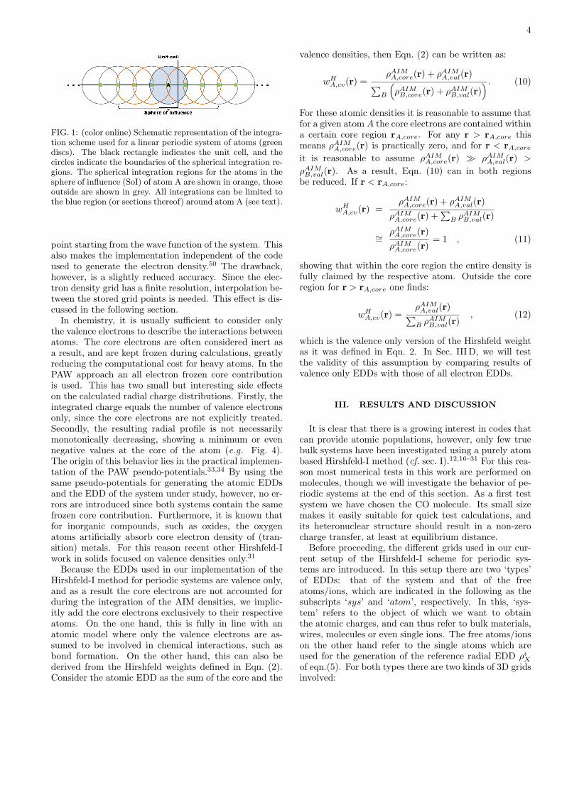
where the sum over all AIS is again an infinite sum. How-ever, in numerical implementations for periodic systems,the exponential decay of the atomic EDD allows us totruncate both the infinite sum and integration regionof Eq.(9), without significant loss of numerical accuracy.The sum can be reduced to contain only the atoms in-cluded in the SoI of atom A (orange circles in Fig. 1),because only these atoms contribute significantly to thedensity in the integration region around atom A. In ad-dition, the integration region for all atoms in the SoI canbe reduced even further, without loss of accuracy, to onlythe region that overlaps with the spherical integration re-gion of atom A (blue shaded disc in Fig. 1).

D. Grid stored electron densities and frozen corepseudo-potentials.

In periodic systems, the use of PBC allows one to re-duce the system size dramatically. For bulk materials thiseven allows simple systems, such as face-centered cubicCu or Ni, to be represented using single atom unit cells.A useful side effect of such reduced cells is that it is easilypossible and relatively cheap to store the EDD ρsystem(r)on a three dimensional grid covering the unit cell, andthus fully describing the entire infinite system. The useof such precalculated electron density grids speeds upthe Hirshfeld method significantly, since there is no moreneed to calculate the electron density at any given grid

4

FIG. 1: (color online) Schematic representation of the integra-tion scheme used for a linear periodic system of atoms (greendiscs). The black rectangle indicates the unit cell, and thecircles indicate the boundaries of the spherical integration re-gions. The spherical integration regions for the atoms in thesphere of influence (SoI) of atom A are shown in orange, thoseoutside are shown in grey. All integrations can be limited tothe blue region (or sections thereof) around atom A (see text).

point starting from the wave function of the system. Thisalso makes the implementation independent of the codeused to generate the electron density.50 The drawback,however, is a slightly reduced accuracy. Since the elec-tron density grid has a finite resolution, interpolation be-tween the stored grid points is needed. This effect is dis-cussed in the following section.

In chemistry, it is usually sufficient to consider onlythe valence electrons to describe the interactions betweenatoms. The core electrons are often considered inert asa result, and are kept frozen during calculations, greatlyreducing the computational cost for heavy atoms. In thePAW approach an all electron frozen core contributionis used. This has two small but interesting side effectson the calculated radial charge distributions. Firstly, theintegrated charge equals the number of valence electronsonly, since the core electrons are not explicitly treated.Secondly, the resulting radial profile is not necessarilymonotonically decreasing, showing a minimum or evennegative values at the core of the atom (e.g. Fig. 4).The origin of this behavior lies in the practical implemen-tation of the PAW pseudo-potentials.33,34 By using thesame pseudo-potentials for generating the atomic EDDsand the EDD of the system under study, however, no er-rors are introduced since both systems contain the samefrozen core contribution. Furthermore, it is known thatfor inorganic compounds, such as oxides, the oxygenatoms artificially absorb core electron density of (tran-sition) metals. For this reason recent other Hirshfeld-Iwork in solids focused on valence densities only.31

Because the EDDs used in our implementation of theHirshfeld-I method for periodic systems are valence only,and as a result the core electrons are not accounted forduring the integration of the AIM densities, we implic-itly add the core electrons exclusively to their respectiveatoms. On the one hand, this is fully in line with anatomic model where only the valence electrons are as-sumed to be involved in chemical interactions, such asbond formation. On the other hand, this can also bederived from the Hirshfeld weights defined in Eqn. (2).Consider the atomic EDD as the sum of the core and the

valence densities, then Eqn. (2) can be written as:

wHA,cv(r) =

ρAIMA,core(r) + ρAIM

A,val(r)∑B

(ρAIM

B,core(r) + ρAIMB,val(r)

) . (10)

For these atomic densities it is reasonable to assume thatfor a given atom A the core electrons are contained withina certain core region rA,core. For any r > rA,core thismeans ρAIM

A,core(r) is practically zero, and for r < rA,core

it is reasonable to assume ρAIMA,core(r) � ρAIM

A,val(r) >

ρAIMB,val(r). As a result, Eqn. (10) can in both regions

be reduced. If r < rA,core:

wHA,cv(r) =

ρAIMA,core(r) + ρAIM

A,val(r)ρAIM

A,core(r) +∑

B ρAIMB,val(r)

∼=ρAIM

A,core(r)ρAIM

A,core(r)= 1 , (11)

showing that within the core region the entire density isfully claimed by the respective atom. Outside the coreregion for r > rA,core one finds:

wHA,cv(r) =

ρAIMA,val(r)∑

B ρAIMB,val(r)

, (12)

which is the valence only version of the Hirshfeld weightas it was defined in Eqn. 2. In Sec. III D, we will testthe validity of this assumption by comparing results ofvalence only EDDs with those of all electron EDDs.

III. RESULTS AND DISCUSSION

It is clear that there is a growing interest in codes thatcan provide atomic populations, however, only few truebulk systems have been investigated using a purely atombased Hirshfeld-I method (cf. sec. I).12,16–31 For this rea-son most numerical tests in this work are performed onmolecules, though we will investigate the behavior of pe-riodic systems at the end of this section. As a first testsystem we have chosen the CO molecule. Its small sizemakes it easily suitable for quick test calculations, andits heteronuclear structure should result in a non-zerocharge transfer, at least at equilibrium distance.

Before proceeding, the different grids used in our cur-rent setup of the Hirshfeld-I scheme for periodic sys-tems are introduced. In this setup there are two ‘types’of EDDs: that of the system and that of the freeatoms/ions, which are indicated in the following as thesubscripts ‘sys’ and ‘atom’, respectively. In this, ‘sys-tem’ refers to the object of which we want to obtainthe atomic charges, and can thus refer to bulk materials,wires, molecules or even single ions. The free atoms/ionson the other hand refer to the single atoms which areused for the generation of the reference radial EDD ρi

Xof eqn.(5). For both types there are two kinds of 3D gridsinvolved:

5

1. Linear grids: Instead of using the analytical expres-sion for the underlying wave function, we use theEDDs stored by VASP on a finite numerical grid.These grids span a single unit cell and use uni-formly spaced grid points in direct coordinates.51(cf. Sec.III A) In the remainder, the following no-tation is used:

• Vatom : The linear grid for the referenceatom density distributions as obtained fromthe atomic calculations.

• Vsys : The linear grid for the (poly)atomicsystem under study

2. Spherical grids: These are atom centered gridswhich are not limited to a single unit cell. Thespherical grids decompose into a radial and a shellgrid. In our current setup, a logarithmic grid isused as radial grid, such that closer to the corethe grid is sufficiently dense to describe this re-gion accurately. The number of radial points waschosen to equal the numbers suggested by Becke.41At each point in this radial grid, a shell is locatedon which grid points are distributed according toa Lebedev-Laikov grid.42 (cf. Sec. III B) The totalnumber of grid points S equals the sum over allatoms of the number of radial points (RA) usedfor that atom times the number of points on eachshell (σ): S =

∑ARA · σ. In the remainder only σ

is varied to study the stability of the integrations.Two three-dimensional spherical grids are distin-guished:

• Satom : Total spherical grid used to generatethe reference spherically averaged radial den-sity distribution for the atoms.

• Ssys : The multi-center spherical grid for thesystem under study.

Note that the results of the Hirshfeld-I AIM analysis de-pend directly on Ssys but also indirectly on Satom as thisdetermines the quality of the isolated atomic EDDs.

A. Electron density grids Vsys and Vatom

As was mentioned in the previous section, the use ofprecalculated grid-based EDDs introduces small inaccu-racies due to the need for interpolation between the ex-isting grid points. The charge of the C atom in a COmolecule as a function of the grid spacing used in theVsys grid is shown in Fig. 2. The different curves arefor different grid spacings used in the Vatom grids, fromwhich the atomic radial EDD ρi

C(niC , r) and ρi

O(niO, r)

are generated. It clearly shows the influence of both gridsto be independent, since all curves have the same shape.Looking in detail at the exact numbers reveals that forboth grids the same accuracy is obtained (cf. Table I).This means that the same change in population of the

FIG. 2: The Hirshfeld-I charge for the C atom in a COmolecule as function of the Vsys grid resolution. The dif-ferent curves show the results for the use of different resolu-tions in the Vatom grids, used for generating the atomic radialdensities. In all molecular calculations we used spherical in-tegration grids of 1202 grid points per shell.

TABLE I: Differences in the Hirshfeld-I populations shown inFig. 2. The presented change in population is the differencein population going from Vsys/Vatom grids with I grid pointsper A, to grids with J grid points per A. The respective gridchanges are indicated as ∆I

J .Top table: Differences along the curves shown in Fig. 2.Bottom table: Differences between the curves shown in Fig. 2.

Vsys Vatom (grid points/A)10 20 30

∆1020 0.00738 0.00743 0.00744

∆2030 0.00126 0.00128 0.00128

∆3040 0.00049 0.00048 0.00049

Vsys Vatom

(grid points/A) ∆1020 ∆20

30

10 -0.00617 -0.00112

20 -0.00612 -0.00111

30 -0.00610 -0.00111

40 -0.00611 -0.00110

C atom in CO is observed when either the Vatom or theVsys grid is changed in an identical way; i.e. the changein the population (in absolute value) of the C atom iscomparable when going from the black to the red curveand when going from a point at 10 grid points per A to apoint at 20 grid points per A on the same curve in Fig. 2.Figure 2 and Table I also show that quite a dense meshis needed to obtain very accurate results. Though this isnot a big problem for periodic systems with small unitcells, it could become problematic for molecules which re-quire big unit cells to accommodate the vacuum required

6

FIG. 3: (a) Convergence behavior of the population/chargeas function of the number of grid points per spherical inte-gration shell. For the C(black line) and O(red line) atom ofthe CO molecule the value shown is the absolute value of thedifference between the calculated population and the calcu-lated population using the most dense grid. In case of the Catom in the diamond system (green line) the charge shouldbe zero, so the absolute value of the calculated charge is pre-sented. (b) The total number of grid points as function of thenumber of Lebedev-Laikov grid points per spherical shell.42

The large number of grid points for the diamond system, isdue to its large SoI (see text).

to prevent interaction between the periodic copies. Thesame is true for high accuracy Vatom grids, which arerequired for generating high accuracy atomic radial den-sities. Fortunately, these must only be calculated once,and the resulting high resolution radial densities can thenbe stored in a small size library containing only r depen-dent densities. In sec. III C the atomic radial EDDs arediscussed in more detail.

B. Spherical integration grids Ssys and Satom

Because the populations and charges in the Hirshfeld(-I) approach are obtained by integration of the EDD of thesystem, attention needs to be paid to the integration gridused. The current implementation uses a multi-centeredgrid, as was noted in Sec. II C. In this setup we used

Lebedev-Laikov grids on the spherical shells of the inte-gration grids.42 Figure 3a shows the influence of the num-ber of grid points per spherical shell on the accuracy; notethe log-log scale used. In general, a denser grid resultsin a more accurate value for the population. However,different atoms in the same system, and the same calcu-lation can show different convergence, as is shown by thecurves of the C and O atoms of a CO molecule. To havethe population of the system atoms converged to within0.001 electron a few hundred grid points per shell are re-quired. For a molecular calculation the multi-center grid,Ssys, only requires a few tens of thousands of grid points,as is seen in Fig. 3b. However, a Hirshfeld-I calculationfor a bulk material such as diamond, which also has onlytwo atoms in its unit cell, requires a multi-center gridSsys with several tens of millions of grid points. Thisdifference by a factor thousand originates from the factthat the SoI for the diamond unit cell contains a fewthousand atoms, which all contribute to the total num-ber of grid points that need to be evaluated. This makesit very important to reduce the SoI as much as possiblesize without significant loss of accuracy.

C. Atomic radial EDDs

The atomic EDDs are calculated in a periodic cellunder PBC, and stored on 3D electron density gridsVatom (cf. Sec. III A). The atomic radial EDDs areobtained from these through spherical averaging of thedensity distributions. Spherical averaging is done usingthe Satom grid, with spherical shells containing Lebedev-Laikov grids of 5810 grid points.42 The resulting distri-butions for different C ions are shown in Fig. 4a. Thepopulations obtained by spherical integration over thesedistributions shows that the correct populations are ob-tained for the neutral and the positively charged ions. Incontrast, the negatively charged ions show a populationwhich is too small. Moreover, the curves in Fig. 4a in-crease again for longer ranges. At first glance, one mightattribute this behavior entirely to the overlapping tailsof periodic copies in neighboring cells. However, a roughextrapolation of the decreasing part of the curve (multi-plied with the number of neighboring cells) shows a muchlower electron density at a distance of 10A than is cur-rently the case. The actual origin of the increase lies inthe fact that the plane wave approach used for the atomcalculations can only bind a limited amount of extra elec-trons to a given atom. This amount varies from atom toatom. As a result, it tries to place the excess electrons asfar from the atom as possible. Due to strong delocaliza-tion inherent to plane waves these electrons are spreadout over the vacuum between the atoms, with the highestelectron density at the center of the unit cell; i.e. as farfrom the atoms as possible.

It is interesting to note that this artifact is purely dueto the use of plane waves, which try to smear out theunbound electrons over the entire (empty) space. If one

7

FIG. 4: Atomic radial electron densities ρA(r) calculated from grid stored atomic charge distributions. (a) Radial electrondensities for different carbon ions obtained from charge distributions in a cubic periodic unit cell of 20.5 × 20.5 × 20.5A3.The populations (pop) given of each ion are calculated by spherical integration of this radial distribution. (b) Radial chargedistributions for two negative carbon ions obtained from the same size periodic unit cell as (a), but with different grid spacings:210, 420, and 630 grid points per 20.5A. (c) Radial EDDs for different hydrogen ions. For the H− and H2− ions the results fordifferent unit cell sizes are compared: 20× 20× 20A3, 30× 30× 30A3, and 40 × 40 × 40A3.

uses a (finite) Gaussian basis set instead, the additionalelectrons are ‘bound’ by definition through the basis setused, even if these electrons should not be bound to theatom anymore. In addition there looms also a concep-tual dilemma: should one use such ‘artifacts’ as referencestates or should one avoid them and restrict oneself onlyto reference systems that can exist. For example, takethe O2− anion. In the gas phase, the second electronis unbound by over 8 eV and one may suggest to usethe O – electron density instead. However, the computa-tional repercussion of this would be that the Hirshfeld-I method would become unstable for systems where ahigher charge is found than is available as ground statefree anion. This behavior and conceptual dilemma is notunique to Hirshfeld-I. Other approaches using externalreference atomic densities suffer it too, since it is inherentto the generation of external atomic reference densities(e.g. DDEC-code,12 although this is not investigated bythose authors). Some other approaches, like the iterativestockholder approach (ISA) of Lillestolen and Wheatley,appear to sidestep this dilemma by generating referenceatomic densities as part of the iterative process.10,11 Thedrawback, in comparison to Hirshfeld-I, of such an ap-proach is that the transferability of the reference atomsis lost. Also, the physical meaning of the reference atomin ISA becomes unclear. On the other hand, the ISAapproach shows that the reference atomic densities areto be considered first and foremost ‘tools’. This shouldalleviate the pressure on our conceptual conscience a lit-tle. Returning to the atomic reference densities used in

Hirshfeld-I, it is possible to define them as the density offree ions in the gas phase. This definition is then softenedsuch that also useful densities can be obtained beyondthe range of ground state ions in the gas phase. This canbe done in several ways: using meta-stable anion densi-ties, binding the additional electrons through the basisset (Gaussian approach), or keeping the shape-functionof the first anion and scaling it in an appropriate waysuch that the required number of electrons is found onintegration. These last two methods correspond to theapproaches presented at the beginning of this section.

From the modeling point of view one might prefer thislatter type of pragmatism over the former, since we areinterested in the EDD of the electrons for ‘free ions’, ir-respective of their bound or unbound nature. Later inthis section we will show how this delocalization problemcan be solved in a simple way.

Fig. 4b shows that this artifact is independent of theresolution used for the Vatom grid, as the different curvesnicely overlap. Fig. 4c shows the influence of the periodiccell size on this artefact. In case of the presented hydro-gen ions, it shows that using a cubic periodic cell with aside of 20A, the curves for H− and H2− coincide in theshort range region. Moreover, they don’t show the ex-pected exponential decay, and increase sharply at longerrange. Using a larger unit cell appears to solve theseproblems: firstly, the radial distributions for the two an-ions become distinguishable, and show the expected ex-ponential decay. Secondly, the point where the excesselectrons start to interfere noticeably is pushed back to

8

FIG. 5: Correlation plots of the charges obtained using theperiodic Hirshfeld-I implementation and the standard all elec-tron molecular implementation: (a) using the atomic radialdensity distributions of set R2 with the corrected tails, (b)using the R3 set with the corrected tails and normalized dis-tributions assuming correct shape functions, and (c) usingthe R4 set with corrected tails and anion distributions nor-malized assuming piecewise linear interpolation of fractionaldensities (see text). In each case the VASP optimized geom-etry was used for the VASP based Hirshfeld-I calculations,while Gaussian optimized geometries were used for the refer-ence calculations.

a larger distance. At this point it is interesting to notethat for the DDEC-code this problem is not mentioned,although the references densities in the c1 method appear

to be obtained in the same fashion as presented here.12Furthermore, from Fig. 4 it is clear that large unit cellsare required for calculating correct radial reference densi-ties for anions. For both C and H anions it is shown thata significant charge density is still present at a distance of7–10A from the nucleus making unit cells of 20× 20× 20A3 necessary to prevent additional overlap errors.

This type of behavior is seen for all atom types investi-gated, positive up to neutral ions give the expected radialdistributions, while the negative ions seem hampered bythe fact that only a fraction of the additional electronscan be attached to the atom. Fluorine and chlorine arein this respect exceptional since for these atoms also theF− and Cl− ions give good distributions and populations.This could be considered a result of the high electronaffinity of these elements.

We find that for most negatively charged ions thepopulations are too small.52 As a result, the calculatedHirshfeld weight wH

A (r) for a negatively charged AIMA is underestimated. The easiest way to compensatefor this discrepancy is by scaling these specific distri-butions such that the correct population is found afterintegration. This way the shape function of the curveis maintained,53,54 but the resulting weights wH

A (r) in-crease. Another possible approach is based on the as-sumption that the fractional density is piecewise linearbetween integer charges.9,55,56 This gives rise to an al-ternative way of normalizing the anion radial densitiesto present the correct integer charges. To investigate theeffects of such a normalization and the erroneous tailsshown in Fig. 4, we compare the results of four typesof atomic radial density distributions. To that end, thereference set of molecules previously used in Hirshfeld-Istudies by Bultinck et al.9,35 is used. This set consistsof 168 neutral molecules containing only H, C, N, O, F,and Cl.

The first set of atomic radial EDDs, called R1, con-tains the density distributions as shown in 4a, wherethe radial distribution is obtained from a periodic cellof 20× 20× 20A3.

For the second set, which is referred to as R2, we havecombined these results with the results from a periodiccell of 40 × 40 × 40A3 but with a lower grid resolution.In this case, the central part of the radial distribution istaken from the 20 × 20 × 20A3 unit cell with the highresolution grid and connected to the tail part obtainedfrom the 40 × 40 × 40A3 unit cell. As a result, the highaccuracy for the center part of the distribution is main-tained, and the tail is corrected through the removal ofthe delocalized electron contribution. Note that for thesedistributions, the curves are limited to a distance of 10Afrom the core, i.e. the same maximum radius as is avail-able from the 20 × 20 × 20A3 periodic cells. Becausethe excess tail electrons are not included anymore, thespherically integrated populations of the negative ionsare slightly smaller than they are for the R1 set.

For the third set, R3, the same procedure as for R2is used, but this time the curves are normalized for the

9

negative ions such that the correct population is given onspherical integration of these radial EDDs while retain-ing the original shape function.

The fourth set, R4, is obtained using the same pro-cedure as for R2, fixing the tail part, and like R3 theresulting curves are then normalized for the anions. Inthis case, however, the starting assumption for this laststep is that the fractional density is given by:

ρ(n+ x, r) = (1− x)ρ(n, r) + xρ(n+ 1, r) nεN, xε[0..1],(13)

where n+x gives the fractional population. In the presentsituation, ρ(n, r) represents the density distribution ofthe neutral atom, and ρ(n + x, r) the obtained densitydistribution for the anion. Note that for the ρ(n + x, r)distribution the spurious tail has already been fixed atthis point, resulting in the expected exponentially de-creasing tail. Rewriting Eqn. 14 gives:

ρ(n+ 1, r) =ρ(n+ x, r)− (1− x)ρ(n, r)

xnεN, xε]0..1].

(14)The resulting ρ(n + 1, r) yields the full anion charge ofn+ 1 upon spherical integration.

To test the accuracy of the results obtained in our peri-odic implementation using these four different atomic ra-dial density distribution sets, we compare the results fora large benchmark set of molecules with those obtainedby a Hirshfeld-I implementation based on a molecularprogram (cf. Sec. II A).

First, two sets of calculations are performed to checkthe influence of the geometry on the results. The firstset used the optimized geometries obtained from Gaus-sian calculations, and the second set used optimized ge-ometries obtained through VASP calculations. For bothsets the R1 atomic radial distributions are used. TableII shows that the resulting correlations are nearly iden-tical, despite the small differences in geometries for thetwo sets. Although the correlation coefficients r can beconsidered reasonable, the spread on the C and N datapoints is quite large. Furthermore, the slope of the linearfit of the C and N data is much too big. In both casesthe intercepts are acceptably small.

Looking at the effect of fixing the tail of the atomic dis-tributions, through the use of the R2 set of atomic radialdensity distributions, we see a slight increase in the slopefor the C and N data, but in general the obtained valuesfor the correlation, intercept and slope remain compara-ble to the previous sets of calculations. For the resultsobtained with the R2 radial distributions, Table II alsoshows the standard deviation of the difference betweenour calculated results and those of the reference data.The values of these standard deviations are similar forthe first two sets, which are therefore not shown. Ta-ble II shows the deviation for the C and N data sets tobe one order of magnitude larger than for the other ele-ments. It is unclear to the authors why specifically thesetwo elements show such a bad behavior. Looking at theunderestimation of the atomic population for the mono-

FIG. 6: Comparison of Hirshfeld-I charges for a set of 168molecules using pseudo valence densities (method R4) and allelectron (AE) valence+core densities.

valent anions we find an error of roughly 0.5e for H andN, and 0.3e for C and O. On the other hand for F andCl an underestimation of 0.1 and 0.0e, respectively, isfound. The only aspect in which C and N differ from theother elements is that both can show large positive andnegative charges.

The correlation results of the R3 atomic radial den-sity distributions show a clear improvement over the pre-vious results. For each data set the slope is closer tounity, though the intercepts remain as before. Especiallythe C and N results show a large improvement. Theirstandard deviation gets halved which is clearly visible inthe correlation plots in Fig. 5a and b. This immediatelyshows that the simple scaling used for fixing the under-estimated population due to the delocalization problemdoes not introduce large artifacts. In contrast, it actu-ally suggests that the shape function of the radial EDDof the negatively charged ions contains roughly the sameinformation as the Gaussian all electron EDD.

The results obtained with the R4 set show even betterresults. The correlation plot in Fig. 5c shows improvedslopes for the C and N data. The slopes presented inTable II are closer to unity for nearly all elements, whilesmall values for the intercepts are retained. The corre-lation and the standard deviation, however, have stayedroughly the same in comparison to the results of the R3set. This shows that the R4 set can be used as a goodapproximation for the gaussian all electron EDDs.

D. Inclusion of core electrons

From Eqs. (10)–(12) it was deduced that the atomiccore density can be exclusively added to the atom it orig-inates from. Furthermore, it was show that only the va-lence electrons are shared between different atoms, givingrise to the obtained atomic charges, in line with chemi-cal intuition. To test the validity of this deduction, we

10

TABLE II: The fitting and correlation results for the different sets of radial EDDs used in Hirshfeld-I calculations for a set of168 molecules. The molecular geometries are either optimized with Gaussian or VASP. The radial distributions R1 are thedefault distributions obtained from VASP atomic density distributions. The radial distributions R2 contain a fix for the tailof the distribution, and the radial distributions R3 contain a fix for the tail of the distributions and in addition the resultingdistributions are normalized to give the correct number of electrons (see text). The radial distributions R4 contain the same tailfix as R2 and R3, but the normalization makes use of the assumption that fractional densities show a piecewise linear behavior(see text). a and b are the slope and the intercept of the linear fit. r is the correlation with Gaussian molecular results, and σgives the standard deviation.

Gaussian geometry VASP geometryR1 R1 R2

a b r a b r a b r σH 1.187 −0.014 0.940 1.208 −0.019 0.944 1.185 −0.008 0.933 0.026C 1.353 0.020 0.966 1.344 0.026 0.970 1.439 0.020 0.963 0.181N 1.454 0.026 0.978 1.455 0.018 0.979 1.483 0.025 0.975 0.154O 1.131 0.066 0.992 1.123 0.057 0.991 1.152 0.064 0.992 0.031F 1.110 0.064 0.982 1.150 0.072 0.977 1.197 0.070 0.981 0.011Cl 1.117 −0.009 0.979 1.124 −0.018 0.980 1.110 −0.013 0.966 0.015

VASP geometryR3 R4

a b r σ a b r σH 1.109 −0.021 0.979 0.016 0.997 −0.016 0.980 0.014C 1.131 0.014 0.989 0.086 1.027 0.003 0.991 0.057N 1.161 0.033 0.995 0.072 0.967 0.052 0.995 0.031O 1.025 0.048 0.993 0.019 0.947 0.042 0.984 0.027F 1.162 0.071 0.987 0.009 1.131 0.064 0.974 0.013Cl 1.072 −0.018 0.993 0.007 1.024 −0.032 0.979 0.011

have calculated the atomic charges for the set of bench-mark molecules using the total all electron densities, andcompared the results to those obtained with the R4 ref-erence densities. Reference all electron core and valencedensities are obtained in a similar way as before, and aresummed to provide full all electron reference densities.57The same is done for the system EDDs, i.e. all elec-tron core and valence densities are added to result in fullall electron EDDs. As can be seen in Fig. 6, the ob-tained Hirshfeld-I charges for the valence calculations ofthe previous section, show excellent agreement with thefull all electron results. The differences in the obtainedatomic charges are generally below 0.01 e, and alwayssmaller than the differences due to the use of a too coarseVsys grids. This clearly shows the assumption based onEqs. (10)–(12) is a valid one to make.

E. Periodic systems

In this final section some actual periodic systems areconsidered. The choice of the example systems is suchthat they can be used to verify that the obtained resultsare reasonable. As such these systems are in essencequite trivial. If they were not, then any results presentedwould be meaningless numbers, unless reference valuesare available in literature, of which there are at thetime of writing very few. One might be tempted touse indirect ways of trying to verify the results (e.g.ESP fitting), but this generally complicates matters and

FIG. 7: Ball-and-stick representations of (a) the cubic dia-mond super cell, (b) the graphene sheet (unit cell indicatedwith black parallelogram), (c) graphite (unit cell indicated) inblack, (d) the cubic CeO2 super cell, and (e) the Ce2O3 unitcell. The black, red and yellow spheres indicate the positionsof the carbon, oxygen and cerium atoms,respectively. The in-equivalent C atoms in the graphite structure are indicated asA and B. The B atoms are always located at the center ofthe hexagons of the neighboring sheets. The inequivalent Opositions in Ce2O3 are indicated as 1 and 2.The ball-and-stick representations are generated using theVESTA visualization tool.58

obfuscates the validity of the results. In addition, small

11

simple systems also keep the obtained results clear. Forthese reasons we have chosen the systems presentedbelow. Their structures are presented in Fig. 7: thesystems of choice are diamond, graphene, graphite,CeO2, and Ce2O3. The diamond and graphene systems,have the property that all C atoms are equivalent, whichshould result in zero charges on all atoms. Graphite isquite similar to graphene, however, two inequivalent Cpositions are present (cf. Fig. 7c). The ceria systems onthe other hand are chosen for the presence of Ce atomswith different valency; tetravalent Ce in CeO2 and triva-lent Ce in Ce2O3. Note that for both systems the sameCe pseudo-potential is used. Furthermore, in CeO2, theO ions are all equivalent, while in Ce2O3 the Ce ionsare equivalent but the O ions are not, only two of themare equivalent. Furthermore, for Ce2O3 we considerboth the ferromagnetic (FM) and anti-ferromagnetic(AF) configurations, allowing us to check how stronglydifferent spin-configurations influence the results in thissystem.

For all these systems we use the radial atomic EDDsof the R3 set, with the Satom spherical integration gridscontaining 5810 grid points per shell. Table III shows thek-point sets used for the periodic systems, the numberof atoms per unit cell and the number of atoms includedin the SoI. The grid point separation for the Vsys gridfor each of these systems was set to ≤ 0.01A. TheHirshfeld(-I) populations are calculated using sphericalintegration grids Ssys with 1202 Lebedev-Laikov gridpoints per shell.

The large number of atoms in the SoI with regardto the small unit cell sizes might make one wonder ifthis method can efficiently be used for larger (moreinteresting) systems. Due to the very nature of the SoIit are the small unit cells which have the highest costper system cell atom. As the system cell grows, therelative weight of the SoI decreases and as a result itbecomes relatively cheap to handle large supercells. Thisis clearly demonstrated in Fig. 8 where the scaling of theCPU time and the SoI is presented for a set of diamondsystem cells of varying size. The smallest cell is the unitcell containing 2 atoms, while the largest cell is a supercell of 128 atoms. Because our implementation does notmake use of symmetry, a system containing 100 equiva-lent atoms is treated the same way as one containing 100inequivalent atoms. This allows us to use the diamondsystem to test the scaling of the implementation. Inaddition, since all supercells present ‘the same system’,an equal number of Hirshfeld iteration are performedfor all supercells to obtain convergence, making themideally suited to check the scaling behavior. As can beseen in Fig. 8, going from the unit cell to the largestsuper cell the SoI roughly doubles, while the systemcell has become 64× larger. On the other hand, theCPU time required for the Hirshfeld-I calculation is onlyincreased roughly tenfold, again showing the beneficialtrend for larger systems. From this it may be clear thatthis method is well suited for large systems, and we

FIG. 8: Scaling behavior of the implemented Hirshfeld-Imethod. Black discs show the SoI in function of the systemcell size (left axis), while the green squares show the requiredCPU time normalized with regard to the unit cell calculation(right axis).

TABLE III: k-point sets and the number of atoms in the unitcell and SoI for the periodic systems under investigation. Inaddition, also the total number of grid points used for thespherical integration grid are given.

k-point set atoms per atoms in grid pointsunit cell the SoI (×106)

diamond 21× 21× 21 2 6374 128graphene 21× 21× 1 2 1276 22graphite 21× 21× 11 4 4618 104CeO2 8× 8× 8 3 3063 69Ce2O3 FM 10× 10× 5 5 3009 77Ce2O3 AF 10× 10× 5 5 3025 78

expect it could easily handle systems containing a fewthousand atoms in the system cell. (Although this mightnot be the case for the solid state or quantum chemistrycode used to provide the required EDDs.)

However, to investigate the obtained results we optedfor small systems. The resulting Hirshfeld and Hirshfeld-I charges for the inequivalent atoms are shown in TableIV. It clearly shows the Hirshfeld values are closer tozero (i.e. the charge at which the atoms are initialized)than the Hirshfeld-I ones. This is the expected behav-ior and its origin was discussed earlier by Ayers1 andBultinck et al.9 The diamond and graphene charges are(nearly) zero as one would expect based on symmetryarguments. This shows there are no significant artifactswhich introduce spurious charges due to the PBC. Theresults for graphite are somewhat remarkable. Table IVshows there is a small charge transfer going from the Ato the B sites. This could be understood as a conse-quence of the very weak bonding between the A sites indifferent sheets. For each C atom, three electrons areplaced in hybridized sp2 orbitals, where the fourth elec-tron delocalizes in distributed π bonds. For the A site

12

TABLE IV: Hirshfeld and Hirshfeld-I charges calculated us-ing LDA generated EDDs. The geometries of the periodicsystems are shown in Fig. 7 where the labels for the inequiv-alent atoms are given.

Hirshfeld Hirshfeld-I(e) (e)

diamond C −0.00007 −0.00007

graphene C 0.00000 0.00000

graphiteCA 0.00113 0.00705CB −0.00115 −0.00707

CeO2Ce 0.59463 2.79393O −0.30091 −1.40056

Ce2O3 FMCe 0.49081 2.32119O1 −0.31318 −1.61119O2 −0.33576 −1.51663

Ce2O3 AFCe 0.48575 2.32755O1 −0.30825 −1.63062O2 −0.33317 −1.51378

C atoms, the contribution to the AIS charge of these πbond electrons is shared between the A sites of neighbor-ing sheets. Since the C atom at the B site has no directneighbor on the neighboring sheet the contribution goesentirely to this atom, resulting in the slightly negativelycharged C atom. Charge neutrality results in a slightlypositively charged C atom at the A site. Similar behaviorwas observed by Baranov and Kohout59 using the Baderapproach. These authors, however, find a larger and op-posite charge transfer, resulting in a charge of +0.08e and−0.08e on the CA and CB atoms respectively. This dif-ference could originate from the different methods used.

The ceria compounds show the behavior expected withregard to equivalent/inequivalent atoms. The Hirshfeld-Ivalues presented in Table IV are comparable with Badercharges presented in literature. Castleton et al. foundfor CeO2 Bader charges of +2.3e and −1.15e for Ce andO, respectively.60 The Mulliken atomic charges for Ce inCe2O3 presented in literature appear strongly dependenton the functional used, varying from +1.29e for PBE upto +2.157e for Hartree-Fock.61,62 The lack of Hirshfeld-Ivalues in the literature makes it difficult to make a truequalitative assessment of our obtained results. However,our results appear to show an overall qualitative agree-ment with the results obtained from other AIM methods.Table IV also shows there is a clear difference betweenthe tri-and tetra-valent Ce ions, also the different config-urations for the O ions show distinctly different charges.Looking at the relative atomic charges of the Ce and Oatoms in CeO2 and Ce2O3 we find the same relative orderas was found by Hay et al.61 and a difference in atomiccharge for the Ce ions of comparable size. The differentcharges for the tri-and tetra-valent Ce ions might temptone to consider these charges as indicators of the oxida-tion state if not the actual oxidation state of the atoms in-volved. As a result one could then assume that the same

charge in a different configuration would be the result ofthe same oxidation state (cf. concept of transferability).Looking at the charges of the O atoms in both CeO2 andCe2O3 shows this is clearly not the case, since all O atomsformally have the same oxidation state, while the calcu-lated Hirshfeld-I charges vary 0.2 electron. The Hirshfeldcharges on the other hand show a much smaller variationof only 0.03 electron. At this point, it is important tostress that atomic charges do not, as opposed to whatis often assumed, directly reveal the oxidation state, northe valence of an atom. A Hirshfeld(-I) analysis, just likea Bader analysis, can only reveal atomic domains. Theactual valence of an atom can be derived from the local-ization indices, which correspond in the simplest form tointegrating twice the exchange-correlation density overthe same atomic domain.63,64 Delocalization indices areobtained from double integration of the exchange corre-lation density over two different atomic domains.65 Suchmatrices have been less thoroughly explored in solid statecalculations.59

Another interesting point to note is that different spin-configurations have little to no influence on the obtainedcharges. This is seen when comparing the FM and AFconfigurations of Ce2O3. This means that for generat-ing the required system EDDs for Ce2O3 a non-spin-polarized calculation suffices for the study of the system.Note, however, that the single atom calculations used togenerate the reference radial densities are spin-polarized.

IV. CONCLUSION

We have presented an implementation of the Hirshfeld-I method specifically aimed at periodic systems, suchas wires, surfaces, and bulk materials. Instead ofcalculating the electron densities at each point in spaceon the fly using the precalculated wave function ofthe system, we interpolate the electron density from aprecalculated EDD on a dense spatial grid, speedingup the calculation of the density significantly. The useof such grids is possible because PBC allow for the useof a relatively small grid to describe the entire systemaccurately.

Unlike total energy calculations, the number of atomsinvolved can not be fully reduced to only those in theunit cell. Although, the populations only need to becalculated for the atoms in the unit cell, the Hirshfeld-Icalculations require a large ‘sphere of influence’ contain-ing a few thousand of atoms. By selecting only the gridpoints which contribute significantly to the calculations,the computational cost of the used multi-center integra-tion grids can be substantially reduced.

We have shown that the uniform grids used to storeboth the atom and the system EDDs have an equal in-fluence on the accuracy of the final Hirshfeld-I calculatedpopulations, leading to the suggestion of building thelibrary of atomic radial EDDs using as dense as possiblegrids. In addition, we have shown that both different

13

atomic types and different chemical environments giverise to a different convergence behavior as function ofthe spherical integration grid.

The problems observed for the atomic radial EDDsof negatively charged ions are solved in a simple way,and we show that the introduced scaling of the dis-tributions significantly improves the obtained resultsfor the Hirshfeld-I charges. The resulting values fora benchmark set of 168 neutral molecules show verygood agreement with the values obtained by a previousimplementation of the Hirshfeld-I method aimed solelyat molecular systems.

In the final section we have investigated some periodicsystems to show the validity of our implementation.For each of these systems the expected behavior of the

charges is observed. Because of their simplicity thesesystems are ideal test cases for Hirshfeld-I implementa-tions for periodic systems.

V. ACKNOWLEDGEMENT

The research was financially supported by FWO-Vlaanderen, project n◦ 3G080209. This work was car-ried out using the Stevin Supercomputer Infrastruc-ture at Ghent University, funded by Ghent University,the Hercules Foundation and the Flemish Government–department EWI.

1 P. W. Ayers, J. Chem. Phys. 113, 10886 (2000).2 R. F. W. Bader and C. F. Matta, J. Phys. Chem. A 108,

8385 (2004).3 C. F. Matta and R. F. W. Bader, J. Phys. Chem. A 110,

6365 (2006).4 R. G. Parr, P. W. Ayers, and R. F. Nalewajski, J. Phys.

Chem. A 109, 3957 (2005).5 R. S. Mulliken, J. Chem. Phys. 3, 573 (1935).6 R. S. Mulliken, J. Chem. Phys. 23, 1833 (1955).7 F. L. Hirshfeld, Theor. Chim. Acta 44, 129 (1977).8 P. Bultinck, Farad. Discuss. 135, 347 (2007), general Meet-

ing on Chemical Concepts from Quantum Mechanics, UnivManchester, Manchester, England, Sep 04-06, 2006.

9 P. Bultinck, C. Van Alsenoy, P. W. Ayers, and R. Carbo-Dorca, J. Chem. Phys. 126, 144111 (2007).

10 T. C. Lillestolen and R. J. Wheatley, Chem. Comm. pp.5909–5911 (2008).

11 T. C. Lillestolen and R. J. Wheatley, J. Chem. Phys. 131,144101 (2009).

12 T. A. Manz and D. S. Sholl, J. Chem. Theory Comp. 6,2455 (2010).

13 R. F. W. Bader, Chem. Rev. 91, 893 (1991).14 E. Francisco, A. M. Pendas, A. Costales, and M. Garcıa-

Revilla, Comp. Theor. Chem. 975, 2 (2011).15 E. Francisco, A. Pendas, and M. Blanco, Theor. Chem.

Acc. 128, 433 (2011).16 A. M. Pendas, V. Luana, L. Pueyo, E. Francisco, and

P. Mori-Sanchez, J. Chem. Phys. 117, 1017 (2002).17 X. Gonze, B. Amadon, P.-M. Anglade, J.-M. Beuken,

F. Bottin, P. Boulanger, F. Bruneval, D. Caliste, R. Cara-cas, M. Ct, et al., Comp. Phys. Comm. 180, 2582 (2009).

18 M. D. Smith, S. M. Blau, K. B. Chang, M. Zeller,J. Schrier, and A. J. Norquist, Cryst. Growth Des. 11,4213 (2011).

19 E. C. Glor, S. M. Blau, J. Yeon, M. Zeller, P. S. Halasya-mani, J. Schrier, and A. J. Norquist, J. Solid State Chem.184, 1445 (2011).

20 J. Schrier, ACS Applied Materials & Interfaces 3, 4451(2011).

21 O. Leenaerts, H. Peelaers, A. D. Hernandez-Nieves, B. Par-toens, and F. M. Peeters, Phys. Rev. B 82, 195436 (2010).

22 O. Leenaerts, B. Partoens, and F. M. Peeters, Appl. Phys.Lett. 92, 243125 (2008).

23 O. Leenaerts, B. Partoens, and F. M. Peeters, Phys. Rev.B 79, 235440 (2009).

24 M. A. Spackman and D. Jayatilaka, CrystEngComm 11,19 (2009).

25 M. A. Spackman and P. G. Byrom, Chem. Phys. Lett. 267,215 (1997).

26 J. J. McKinnon, A. S. Mitchell, and M. A. Spackman,Chem.-Eur. J. 4, 2136 (1998).

27 J. J. McKinnon, M. A. Spackman, and A. S. Mitchell, ActaCrystallogr., Sect. B 60, 627 (2004).

28 S. K. Wolff, D. J. Grimwood, J. J. McKinnon, D. Jayati-laka, and M. A. Spackman, Crystal explorer 2.1 (2007).

29 T. Watanabe, T. A. Manz, and D. S. Sholl, J. Phys. Chem.C 115, 4824 (2011).

30 G. W. Rogers and J. Z. Liu, J. Am. Chem. Soc. 133, 10858(2011).

31 T. Verstraelen, S. V. Sukhomlinov, V. Van Speybroeck,M. Waroquier, and K. S. Smirnov, J. Phys. Chem. C 116,490 (2012).

32 D. E. P. Vanpoucke, HIVE v2.1, http://users.ugent.be/

~devpouck/hive_refman/index.html (2011).33 P. E. Blochl, Phys. Rev. B 50, 17953 (1994).34 G. Kresse and D. Joubert, Phys. Rev. B 59, 1758 (1999).35 S. Van Damme, P. Bultinck, and S. Fias, J. Chem. Theory

Comput. 5, 334 (2009).36 P. Hohenberg and W. Kohn, Phys. Rev. 136, B864 (1964).37 W. Kohn and L. J. Sham, Phys. Rev. 140, A1133 (1965).38 J. C. Slater, The Self-Consistent Field for Molecular and

Solids, vol. 4 of Quantum Theory of Molecular and Solids(McGraw-Hill, New York, 1974).

39 S. H. Vosko, L. Wilk, and M. Nusair, Can. J. Phys. 58,1200 (1980).

40 M. J. Frisch, G. W. Trucks, H. B. Schlegel, G. E. Scuseria,M. A. Robb, J. R. Cheeseman, J. A. Montgomery, Jr.,T. Vreven, K. N. Kudin, J. C. Burant, et al., Gaussian 03,Revision E.01, Gaussian, Inc., Wallingford, CT, 2004.

41 A. D. Becke, J. Chem. Phys. 88, 2547 (1988).42 V. I. Lebedev and D. Laikov, Doklady Mathematics 59,

477 (1999).43 E. R. Davidson and S. Chakravorty, Theor. Chim. Acta

83, 319 (1992).44 E. Francisco, A. M. Pendas, M. A. Blanco, and A. Costales,

J. Phys. Chem. A 111, 12146 (2007).

14

45 P. W. Ayers, R. C. Morrison, and R. K. Roy, J. Chem.Phys. 116, 8731 (2002).

46 P. Bultinck, P. W. Ayers, S. Fias, K. Tiels, andC. Van Alsenoy, Chem. Phys. Lett. 444, 205 (2007).

47 D. Ghillemijn, P. Bultinck, D. Van Neck, and P. W. Ayers,J. Comput. Chem. 32, 1561 (2011).

48 G. Voronoı, Journal fur die Reine und Angewandte Math-ematik 133, 97 (1907).

49 E. Wigner and F. Seitz, Phys. Rev. 43, 804 (1933).50 In theory, one might even use electron density data deter-

mined from X-ray crystallography. In that case however,there would be the problem of the choice of the atomic ref-erence densities. One would have to use all electron atomicradial densities, which in itself is not really an issue. Thechoice of the functional, however, would be a bit of a wildcard. Actual tests will have to be performed to investi-gate how significantly this choice influences the obtainedresults.

51 In our setup we use the CHGCAR-file produced by VASPas input. Due to it’s simple format this means that compa-rably formatted input can easily be generated for differentsolid state codes, making our setup independent of the usedsolid state/quantum chemical code.

52 Note that for the DDEC-code no such corrections are men-tioned for the similar c1 method. The effect of using suchunder-populated reference anions is shown by comparisonof Fig. 5a to Fig. 5b or c.

53 R. G. Parr and L. J. Bartolotti, J. Phys. Chem. 87, 2810(1983).

54 R. G. Parr and W. Yang, Density-Functional Theory ofAtoms and Molecules, vol. 16 of International series ofmonographs on chemistry (Oxford Science Publications,Oxford, 1989).

55 J. P. Perdew, R. G. Parr, M. Levy, and J. L. Balduz, Phys.Rev. Lett. 49, 1691 (1982).

56 W. Yang, Y. Zhang, and P. W. Ayers, Phys. Rev. Lett. 84,5172 (2000).

57 VASP allows for the generation of all electron core (AEC-CAR0) and valence (AECCAR2) densities.

58 K. Momma and F. Izumi, J. Appl. Cryst. 41, 653 (2008).59 A. I. Baranov and M. Kohout, J. Comput. Chem. 32, 2064

(2011).60 C. W. M. Castleton, J. Kullgren, and K. Hermansson, J.

Chem. Phys. 127, 244704 (2007).61 P. J. Hay, R. L. Martin, J. Uddin, and G. E. Scuseria, J.

Chem. Phys. 125, 034712 (2006).62 J. Yang and M. Dolg, Theor. Chem. Acc. 113, 212 (2005).63 R. F. W. Bader and M. E. Stephens, J. Am. Chem. Soc.

97, 7391 (1975).64 R. Ponec and D. L. Cooper, Faraday Discuss. 135, 31

(2007).65 P. Bultinck, D. L. Cooper, and R. Ponec, J. Phys. Chem.

A 114, 8754 (2010).