1

WHAT DRIVES EXPORT SURVIVAL?

AN ANALYSIS OF EXPORT DURATION IN LATIN AMERICA

Tibor Besedes Juan Blyde Georgia Institute of Technology Inter-American Development Bank

January 2010

ABSTRACT

Statistical techniques from survival analysis have recently been applied to explore the duration of trade relationships (Besedes and Prusa, 2006a, 2006b, 2007). Among the findings from this new literature is that trade relationships are remarkably brief. In this paper we provide evidence confirming that export relationships are in general short-lived but that significant differences across regions exist with Latin America exhibiting lower export survival rates than the US, the EU and East Asia, among others. Counterfactual exercises show that raising export survival rates in Latin America to the levels observed in other regions can produce fairly large increases in exports over the long run. In the second part of the paper we test a battery of possible correlates of trade duration to analyze what factors help explain the differences in survival rates. The findings point to a number of aspects with potential policy implications for the countries in Latin America. JEL No. F1 Key word: Survival, duration, export growth, specialization

2

I. Introduction

In recent years, a growing body of reserach has stressed the importance of export discovery for

developing countries. Hausmann and Rodrik (2003) argue that developing countries facing

shortcomings in learning what they are good at producing (or “self-discovery”) is an important

explanation for their limited export success. Hausmann, Rodriguez and Wagner (2006) present

evidence showing that the degree of flexibility of the economy – measured by its capability to move

production to new goods – is significantly correlated to the length of its economic crises which tend

to be longer in the developing world.

Given its relevance to export growth and development, several studies have been devoted to

better understand the process of export discovery. Hausmann and Klinger (2006) explain differences

in the rate of structural transformation and diversification across countries as a function of input

linkages between sectors. Klinger and Lederman (2006) show that empirical measures of entry costs

affect patterns of new export discovery.

Although the lack of export discovery can be an important factor behind the lack of export

growth in developing countries, some authors have argued that the main reason behind the lack of

export growth in developing countries is not necessarily the failure to discover new export activities

but rather the inability to maintain export relationships (see Besedes and Prusa, 2007). The two

concepts, however, are not necessarily independent. For instance, some of the short-lived export

episodes that we observe might be trials and errors in which the exporter experiments with different

prototypes of the good or in different markets before “discovering” the new successful export

activity.

Stepping aside from this discussion, what is clear is that there is abundant evidence

describing new export attempts in developing countries that fail to survive after a few years of

service. A recent Inter-American Development Bank research project, for example, presents

information about exporters in Latin America that initially succeed in penetrating foreign markets

but fail to maintain their trade relationships after some time (IDB, 2007). Some examples cited in

the project are exports of mangoes in Colombia, office furniture in Brazil, flowers in Ecuador

(during the sixties) and segments of the electronic industry in Uruguay. Episodes in which a country

exports a product for a few years and then stops seem to be far from unusual. This prompts the

3

question of what drives export survival. In other words, why do some export relationships persist

over time while others are only short-lived?

Studies of export duration are a relatively recent phenomenon for several reasons. In most

models of international trade, explicit considerations of the duration of trade are normally absent.

The implicit assumption, however, is that once a trade pattern is established it will last for long time.

In most models shifts in the patterns of specialization due, for example, to differences in factor

accumulation, the diffusion of technology or the life cycle of a product, tend to occur only gradually.

Even in models of hysteresis in trade (Baldwin and Krugman, 1989) which explicitly consider the

duration of trade, the stability of trade partnerships is the common assumption. Accordingly, the

general perception has been that trade relationships are long-lived.

Besedes and Prusa (2006a, 2006b), however, found that most US import relationships did

not survive for long. More than half of all trade relationships are observed for only one year and

approximately 80% are observed for less than five years. Short-lived trade relationships have been

found in other studies: Eaton, Eslava, Kugler and Tybout (2007) for the case of Colombian exports,

Volpe and Carballo (2007) for Peruvian exports, and Nitch (2007) for German imports. The

literature on trade duration is still incipient,1 but the empirical findings so far suggest that short-lived

trade episodes are far more common than initially thought and clearly not limited to the developing

world. This is also confirmed by a recent study of manufacturing exports of 46 developed and

developing countries which shows the median survival to be just 1-2 years (Besedes and Prusa,

2007). Particularly relevant is the finding that although trade relationships are short-lived in general,

there are differences among regions. The hazard rates of Latin American exports are normally higher

than the corresponding hazard rates in other countries. Another relevant finding is that even small

differences in survival rates could account for large differences in export growth in the long-run.

The possibility that a low survival rate may be at the core of the mediocre overall export

performance of Latin American countries relative to other countries deserves a closer. In this study

we compare duration of exports of Latin American economies to those of several other countries

and examine the determinants of differences in survival.

The rest of the analysis is divided as follows. Section II describes data and presents some

relevant statistics. Section III sketches the basic concepts of survival analysis applied to trade data

and shows the empirical strategy that is followed throughout the paper. Section IV shows the

1 There is also a recent related literature that studies the duration of pricing of traded goods. Gopinath and Rigobon (2006), for instance, analyze the stickiness of pricing of US imports and exports.

4

typology of export survival in Latin America and presents benchmark comparisons. Section V

performs counterfactual exercises to calculate the potential growth rate of exports in Latin America

under alternative survival rates. Section VI proceeds to estimate several regression models for

survival data to analyze what factors help predict the hazard rate of exporting. The decomposition of

the regional differences in export hazard rates among the covariates is also presented in this section.

Finally, section VII concludes with a discussion of the results and their implications.

II. Data Description

The choice of data aggregation is particularly important for any analysis of duration of trade.

In general, periods of continued trade tend to become longer the more aggregated the data is

because the wider the range of products that are covered by an industry classification, the higher is

the probability that at least one product is traded in that category for a given year (see Besedes and

Prusa 2006a). On the other hand, at a very detailed level of product disaggregation, even a minor

change of product specifications may lead to a reclassification of an otherwise identical product,

which would result in a recorded failure of a trade relationship. Potential modifications of product

codes over the years may affect the results more strongly when using highly disaggregated data.

Finally, concerns about data quality and the presence of missing values, particularly for developing

countries and for early decades, become more of an issue with more disaggregated data. Given these

considerations, we use data recorded at the 4-digit level of SITC revision 1 between 1975 and 2005.

This provides us with the longest time series of data as well as higher quality than the 5-digit level.2

Accordingly we analyze the period 1975-2005. We focus on manufacturing and not agriculture

because the most important implications for growth strategies in Latin American countries

fundamentally target the manufacturing sector. We restrict our attention to the following SITC

industries Chemicals (SITC=5), Manufactured Materials (6), Machinery (7), and Miscellaneous

Machinery (8). Data come from the UN Commodity Trade Statistics Database (UN Comtrade). We

also perform the analysis with a more disaggregated data recorded at the 6-digit HS level. Since the

Harmonized System did not become widely used before 1991 or 1994 it gives us a shorter time

series and we use it as a robustness check only.

II.A. Preliminary Look at the Data

2 Especially for the early years in our sample it is often the case that there are more observations at the 4-digit than the 5digit level of SITC.

5

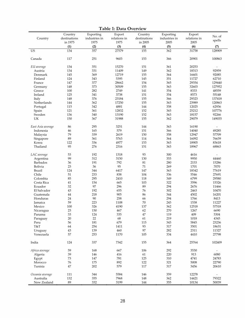
Our benchmark database consists on bilateral trade flows for 47 exporting countries and 157

importing countries over the period 1975-2005. The entire dataset comprises a total of 12,994,907

observations.3 For the HS-6 digit level of aggregation the dataset consists on 44 exporting countries

(the same exporting countries of the 4-digit dataset except for Barbados, Jamaica and Panama that

were eliminated because of lack of data) and the same 157 importing countries. This dataset

comprises a total of 16,674,816 observations. Table 1 presents a preliminary look at the data. In

1975, for example, Peru exported to 56 countries a total of 181 4-digit level activities. The total

number of country-activities pairs (export relationships) that Peru had during this year was 679. In

2005, the corresponding numbers were 115 countries, 343 activities and 5,845 export relationships.

A fundamental part of duration analysis is to measure the length of the export relationship.

That is, the length (in years) that a country exports a particular good to another country. The key

step involves converting the annual raw data into spells of service for each export relationship. For

instance, if a country exports the same good to the same country during ten years, we take this as

one spell of service with a length of 10. Also, if the country exports the same good to the same

country in two (or more) distinct non-overlapping spells of service, for example, during 1985-1994

and then again during 2000-2003, we treat this as two independent spells.4 Our data consists on a

total of 2,580,724 spells. The last column in Table 1 shows the number of spells for each country. In

the next section we discuss in more detail all the statistical techniques of survival analysis applied in

this study.

Table 2 provides some preliminary insights on the issue of export survival. The first column

shows the growth of total exports by countries and regions for the period 1975-2005.5 It is easy to

see that the growth of exports in LAC has been relatively weak, particularly when compared to East

Asia. Column (2) shows the growth rate of export relationships. Once again, the growth rate in LAC

3 The selection of the countries is dictated by data limitations. For example, for the case of the exporting countries, we could not include some of the small countries in Latin America (most of the small islands in the Caribbean, for example) because of a lack of data covering the entire period. Nevertheless, we include 20 countries of Latin America representing more than 90% of the region’s GDP. The other exporting countries serve as comparators, which include nations from the EU, East Asia, Oceania, Africa and North America. Regarding the importing countries, we would have liked to add all countries. However, some countries had to be eliminated from the analysis because of the particular changes that they experienced that impede us to track their import flows over time. For example, Comtrade reports data on U.S. exports to Georgia, an ex-Soviet Republic, starting from 1992. Before 1992, Comtrade reports U.S. exports to the entire “Soviet Union.” As it is not possible to know what part of exports from the US to the Soviet Union went to Georgia between 1975 and 1992, Georgia is eliminated from the analysis. Likewise, we eliminated all destinations for which it was not possible to track the flows of imports during the entire period 1975-2005. The 157 destination countries that we include in the analysis comprise more than 90% of total exports for any of the 47 exporting countries. 4 We also use alternative methods for handling multiple spells which will be shown later in the analysis. 5 To avoid the presence of outlier years, the growth rate between 1975 and 2005 is calculated using the average of 1975-77 for the beginning of the sample and 2003-05 for the end.

6

pales relative to East Asia.6 This is suggestive of the meager efforts in the region to discover new

export activities and/or new markets. Hausmann and Rodrik (2003) have indeed argued that the

shortcomings at the discovery stage are at the center of the limited export success of developing

countries.

The lack of dynamism in export discovery, however, does not seem to be the only problem

in Latin America. The third column in Table 2 shows the ratio of the growth of exports to the

growth of export relationships. For the US and the EU this ratio is many times larger than for Latina

America. Even for East Asia, a region with an impressive growth rate of export relationships (the

denominator in this ratio), the growth of exports relative to the growth in export relationships is

much larger than for Latin America. A potential explanation for this finding is that export

relationships in East Asia survive for longer periods of time than in Latin America, thus allowing

East Asian relationships to grow more. As we will discuss later, differences in duration account for

very large differences in export performance across these two regions.

III. Empirical Strategy

Using statistical techniques of survival analysis, duration can be modeled as a sequence of

conditional probabilities that a trade relationship continues after t periods given that it has already

survived for t periods. This is the essence of the survivor function. In a similar fashion, the hazard

function is the probability that the trade relationship fails after t periods given that it has survived up

to that point.7

More formally, let T be a non-negative random variable denoting the time to a failure event.

The survivor function of T is:

)Pr()( tTtS (1)

The function is equal to one at t = 0 and decreases toward zero as t goes to infinity. The

hazard function, also known as the instantaneous failure rate, is:

) |Pr()( tTtTth (2)

6 The industrial countries experienced lower growth rates of export relationships during this period than Latin American countries. However, in 1975 these countries already had a stock of discoveries that was larger than Latin America by several orders of magnitude: the EU had a stock of discoveries that was 11 times larger and the U.S. had a stock of discoveries 20 times larger (see Table 1, column 3). Note that it is relatively more difficult to increase the number of export relationships during a given period if a country starts with a large stock of export relationships than with a very low base. At the limit, a country that already exports all 4-digit activities to all countries of the sample cannot expand its export relationships any further, and even if all relationships remain active, by definition, the growth rate would be equal to zero. 7 See Kiefer (1988) for a detailed description of duration analysis.

7

The hazard function can vary from zero (meaning no risk at all) to infinity (meaning the

certainty of failure at that instant).

In practice, the survivor and hazard functions are estimated (non-parametrically) by

computing the number of spells that survive (fail) as a fraction of the total number of spells that are

at risk after t periods. For a dataset with observed failure times, t1…., tk, where k is the number of

distinct failure times observed in the data, the Kaplan-Meier product limit estimator of the survivor

function is:

ttj j

jj

jn

dntS

|

)(ˆ (3)

where nj is the number of spells at risk at time tj and dj is the number of failures at time tj. The

product is over all observed failure times less than or equal to t. Similarly, a non-parametric

estimation of the hazard function is given by the ratio of spells who fail to the number of spells at

risk in a given period t.

j

j

n

dth )(ˆ (4)

The survivor and the hazard functions are alternative ways to express the same underlying

process. We will use both measures throughout the paper.

A common issue in survival analyses is the presence of censored observations. These are the

observations for which there is uncertainty regarding either the beginning or the ending date (or

both) for some trade relationships. In our case, for example, export relationships observed in 1975

are left-censored as they may have started in 1975 or before. Relationships observed in 2005 are

right-censored as the may have truly ended in that year or at a later unobserved time. Both types of

censoring are common in duration analysis and are accounted for in the analytical tools that we use

in the study.

The empirical strategy of the paper is as follows: in section IV, we estimate export survival

functions for several different countries in order to compare how Latin America fares relative to

other regions. In section VI we estimate regression models for survival data to analyze what factors

help explain the differences in the duration of exports. The regression models are normally specified

around the hazard function as these models are more easily grasped by observing how covariates

affect the hazard. In particular we use the semiparametric Cox proportional hazards model proposed

by Cox (1972). The model asserts that the hazard rate for the ith subject in the data is

8

xitxi ethxth )(

0 )() |( (5)

where )(tx contains potentially time-varying covariates, and the regression coefficients x are to be

estimated from the data. In the Cox model the baseline hazard, )(0 th , is left unestimated. This is an

advantage of the Cox model as no assumptions about the shape of the hazard have to be made,

assumptions that might lead to misspecification and mislead results about x .8 The Cox model is by

far the most popular of choices in regressions models for survival data.

IV. Typology of Export Duration

Table 3 presents a first view of the length of export relationships by regions. It is

immediately evident that export relationships are in general brief. The median length of a spell in the

US is 2 years and only 1 year for all the other regions. More nuances appear in survival functions. In

the US 60.7% of export relationships survive the first year, 32.8% survive the first 5 years and only

22.2% survive by the end of 15 years. As low as these numbers may look, they are higher than the

corresponding survival rates in Latin America by more than 10 percentage points. In the Latin

American region, only 47.3% of the export relationships survive passed the first year. This survival

rate is lower than corresponding rates in the US, the EU and East Asia by 13.4, 5.5 and 5.6

percentage points respectively. By the end of 15 years, the differences in survival rates between Latin

America and the US, the EU and East Asia are 12.3, 6.0 and 8.9 percentage points respectively.

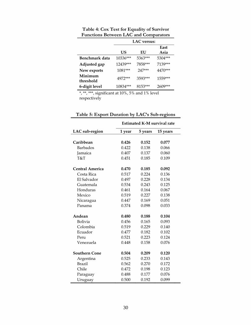
The fact that regional differences across survival functions exist can be tested systematically

through standard tests for equality of survivor functions. Table 4 shows the Cox tests in which the

null hypothesis is that Latin America has the same survival function as the US, the EU and East

Asia, respectively.9 The results for our benchmark data is presented in the first row. All three

hypotheses are easily rejected indicating that there are statistically significant differences between

Latin American survival function and those from the US, the EU and East Asia.

Figure 1 shows the graphical representations of the Kaplan-Meier estimated survival

functions for the four regions. The Latina American survival function is always below that of the

other regions. Note that all survival functions are similar in shape; that is, the survivor functions are

relatively steeper in the early years and relatively flatter later on. This indicates that export

8 The cost, however, is a loss in efficiency; if we knew the functional form of )(0 th , we could do a better job of estimating x . 9 Other tests for the equality of the survivor functions are: Long-rank, Wilcoxon-Breslow-Gehan, Peto-Peto-Prentice and Tarone-Ware. Note that the regional data have been weighted so that each country has the same weight within its own region. The consequence of this weighting is that only the Cox test that can be used to test equality of survivor functions.

9

relationships experience higher risks of failure when they are fairly new with a decreasing the risk as

relationship age. In the case of Latin America, the rate of survival decreases by 15 percentage points

between years 1 and 2, by 7 percentage points between years 2 and 3 and by 4 percentage points

between years 3 and 4. Starting from year 6, the risk of survival decreases by less than 2 percentage

points every year and beginning in year 9 only by less than 1 percentage point. The risks of failure

decrease with age and after some time the risks change only marginally. The result might have some

important policy implications. For instance, any mechanism designed to support export activities

would be particularly important during the early years of service when the risks of failure are high.

After some time, the risks of failure substantially drop and the support might no longer be needed.

Returning to regional comparisons, Figure 1 shows that regardless of the age of the export

relationship, the differences in survival rates between Latin America and other regions persist and

sometimes even increase. The difference in survival rates between Latin America and the EU

increase with the year of service. The same is true of the difference between Latin America and East

Asia.

IV.A. Robustness Checks

We now check whether the results shown in Figure 1 hold under alternative data checks. First, as

mentioned before, some exports relationships reappear, exhibiting multiple spells of service. A

country may export a good to another country, exit the market, then re-enter and possibly exit again.

So far we have treated these multiple spells as different spells of service. However, we can explore

alternative treatments. There is a possibility that some of the reported multiple spells are not

different episodes but the result of a measurement error. For example, if we observed a relationship

between 1980 and 1991 and then again between 1993 and 1995 we treated them as two different

spells of service. However, it could have been the case that the reason we did not observe the

relationship in 1992 was because there was a measurement error. Therefore interpreting the initial

spell as ‘ending’ in 1991 was inappropriate. It is more adequate to interpret the two spells as one

longer spell lasting from 1980 to 1995. This type of error would be particularly problematic if there

is more misreporting in developing countries, particularly in LAC, than in the benchmark regions

because we might be concluding that export survival rates in LAC are lower than what they really

are.

To allow for such misreporting, we follow Besedes and Prusa (2006a) and assume that a one-

year gap between spells is an error, merge the individual spells, and adjust the spell length

10

accordingly. Gaps of two or more years are assumed to be accurate and result in no adjustments.

While more elaborate methods could be employed to adjust the data, this approach is the most

appealing one due to its simplicity particularly when more information on the exact nature of

misreporting is not available. The results are shown in the second row of Table 4, labeled “Adjusted

gap”. The Cox tests performed with the adjusted data indicate that in all the three cases, the null

hypotheses of equality of survivor functions are once again rejected.

Another check we perform is to consider whether the results shown in Figure 1 hold if we

use only the new export activities. We mentioned in Section III that the survival methods used in

this paper address the issues of censoring. Nevertheless, by focusing the analysis on the new exports

activities, we take an extra step in making sure that issues of censoring (in this case, left-censoring)

are not affecting the results in any significant way. We adjust our dataset to consider only new export

relationships that begin in 1976 or later. The third row of Table 4, labeled “New exports” shows the

results of the Cox tests. The three hypotheses of equality of survivor functions are rejected once

again.

We can adjust the data to consider trade flows above some minimum threshold. Minimum

thresholds have been used before to eliminate minor errors in the data or to get rid of values that

might not be meaningful enough to be counted as a trade flow. For instance, in order to explore

whether or not a nation imported a good in a given period, Evenett and Venables (2002), use

minimum thresholds to get rid of what they call “economically unimportant levels of imports”.

Balza, Caballero, Ortega and Pineda (2007) also used minimum thresholds for the same purpose. In

this paper we apply minimum thresholds to explore how robust our results are. Evenett and

Venables use a cutoff value equal to $50,000, meaning that recorded trade flows below $50,000 are

treated as if there was no trade at all. We use three alternative thresholds: $10,000, $30,000 and

$50,000. This means that we drop spells with initial trade smaller than the corresponding threshold.

In the fourth row of Table 4 (labeled “Minimum threshold”) we report the results with the most

stringent threshold, $50,000. As indicated by the Cox tests, all the hypotheses are once again

rejected. Results with the other thresholds are qualitatively similar.

Finally, we report the results when we use the 6-digit HS data. Figure 2 shows the K-M

survival functions for the four regions and the last column of Table 4 presents the results of the

corresponding Cox tests. Even with this alternative dataset we find once again that Latin American

export survival rates are significantly lower than those of the comparators.

11

IV.B. Latin American sub-regions

Table 5 shows the Kaplan-Meier estimates of the survivor function disaggregated by Latin American

sub-regions and countries. Within Latin America, the region that shows the largest survival rates is

the Southern Cone followed by the Andean countries, Central America, and finally the Caribbean.10

The relatively better performance of the Southern Cone is no consolation when compared to our

non-Latin American benchmarks. All four sub-region’s survival rates are lower than the survival

rates of any of the benchmarks. Figure 3, for example, shows the K-M estimated survivor functions

of the four sub-regions and includes the survival function of East Asia for comparison. It is clear

that the four survivor functions lie below the East Asian survival function at any year of service.

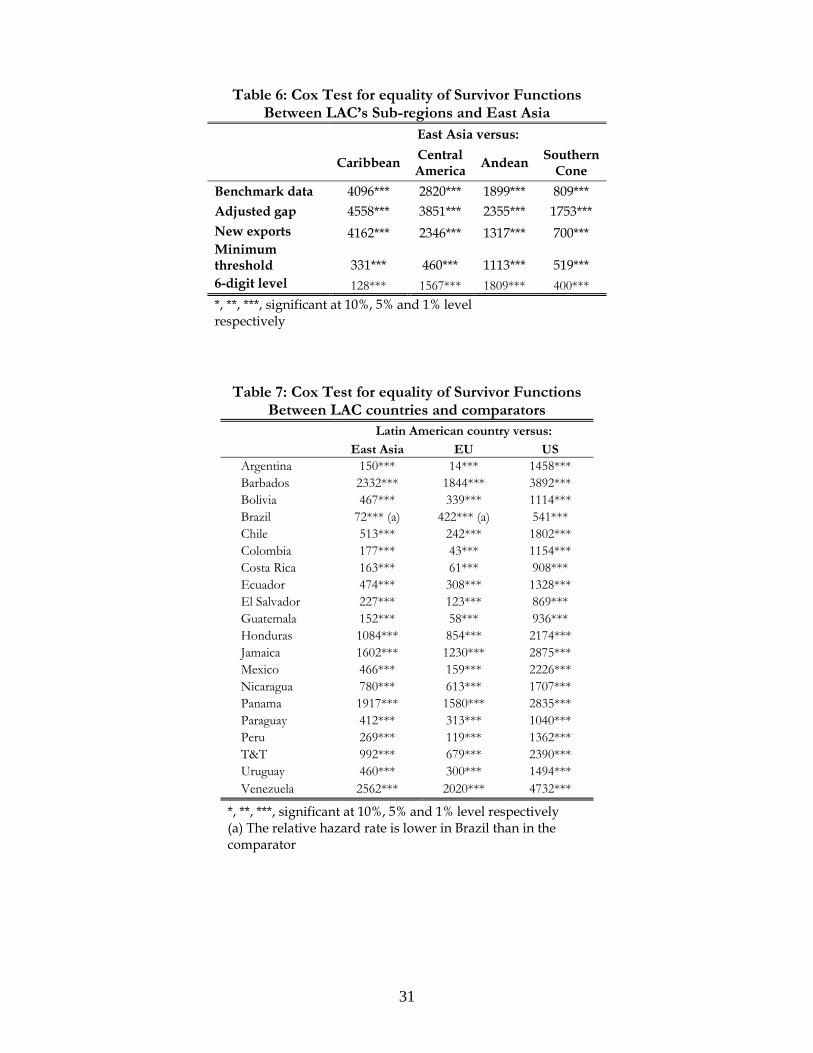
Table 6 shows the Cox tests of equality when using East Asia as a reference. All hypotheses of

equality are easily rejected not only with benchmark data but also when adjusting for 1-year gaps,

minimum thresholds, new exports only, and using the 6-digit HS data. We also arrive to similar

conclusions when using the EU or the US as reference points (not shown in the table).

In Table 7 we show the Cox tests for equality of survival functions for each Latin American

country. According to the tests, all the countries in the region have survival functions with implicit

hazard rates that are statistically significantly higher than that of any of the comparators. The

exception to this is Brazil. Brazil has a survival function that does not lie below the survival function

of either East Asia or the EU. Indeed, according to the Cox tests, the survival function in Brazil has

an implicit hazard rate that is statistically significantly lower than that of East Asia or the EU. This is

not the case, however, when Brazil is compared to the US. Relative to the US, Brazil still compares

unfavorably. All other countries in Latin America have survival functions that are significantly lower

than the survival functions of the three benchmark regions.

Having found that LAC survival rates are consistently below that of other parts of the world,

the natural question to ask is what drives these gaps. One possibility is differences in specialization

patterns. The export baskets of LAC are in general biased towards homogeneous goods. Therefore,

the average export survival rate in the region could be lower than in other regions because of a

relative specialization in these goods. Besedes and Prusa (2006b), for example, show that the hazard

rate is at least 23 percent higher for homogeneous goods than for differentiated products. We will

analyze in detail the determinants of survival rates in section VI, but here we provide a brief

preliminary look at this issue.

10 A Cox test of equality of survival functions indicates that the four functions are indeed statistically different at 1% level.

12

We aggregate all 4-digit level activities in 3 categories according to Rauch’s (1999)

classification: homogenous, differentiated and an intermediate category called reference products.11

Then we estimate separate Kaplan-Meier survivor functions for each product category. Figure 4

shows the results. The probability of survival is always the highest for differentiated products and

always the lowest for homogeneous goods. The hypothesis that these three functions are equal is

rejected at the 1% significance level with the Cox test. This indicates that there are indeed

differences in survival rates across sectors categories. Regarding the biases of the export baskets, our

data shows that exports of differentiated products represent 84% of total exports in East Asia while

73% in LAC.

Given the above two results, one is tempted to conclude that the lower average export

survival rate in Latin America is the result of its specialization patterns with relatively lower export

shares in differentiated products. However, although this is in part true, there is more than meets the

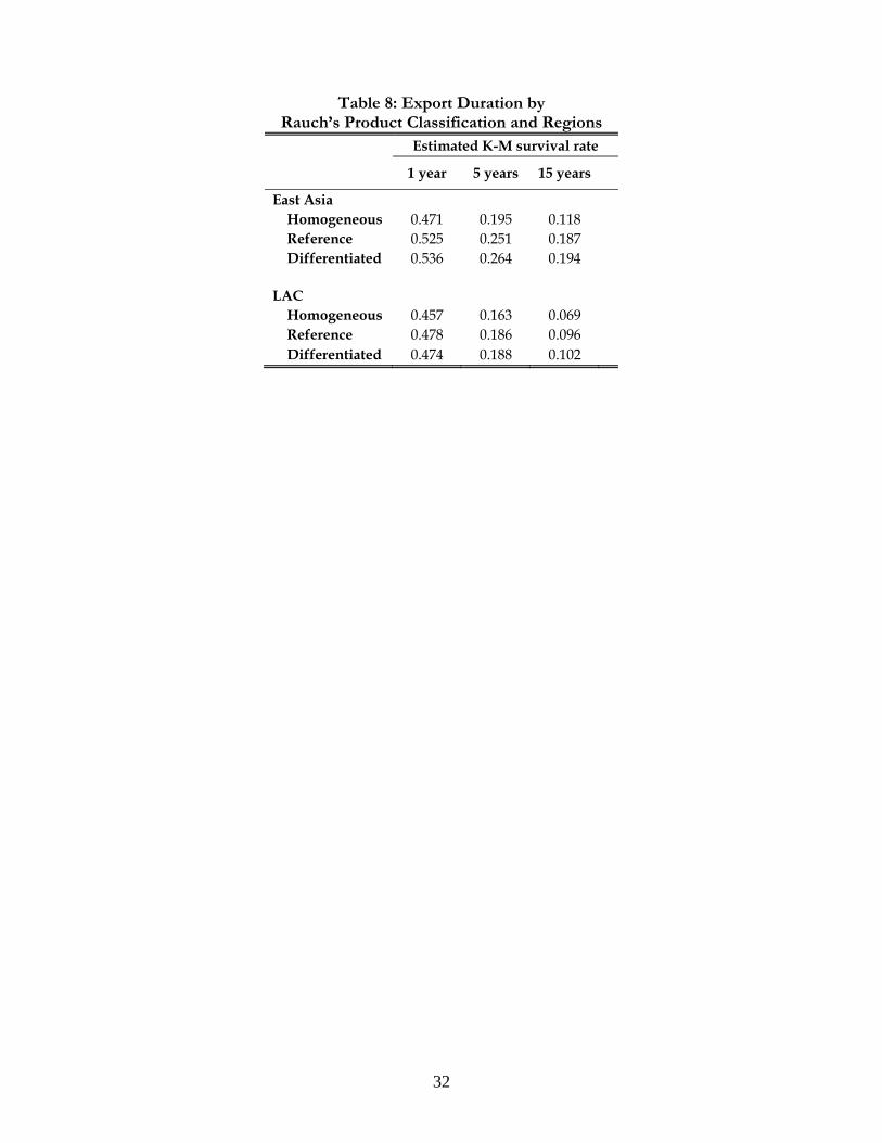
eye here. In Table 8 we report again the export survival rates by product classification but also by

regions. The main finding is that export survival rates in East Asia are higher than in Latin America

for all three types of goods.12 East Asia has sustained higher survival rates than Latin America in

differentiated products, in referenced and in homogeneous goods. Therefore, even if East Asia

would have had the same specialization pattern as Latina America, its average export survival rate

would have still been higher. The way we interpret this result is that differences in the average

survival rates across the regions might not be solely the result of differences in specialization

patterns but that other factors might be playing a role as well. As mentioned before, we will address

this issue in detail in section VI where we investigate the determinants of export survival rates with

the help of an econometric model.

Before turning to the determinants of export survival, we would like to get an estimate on

what Latin America is likely to gain in terms of export growth if export survival rates were to

increase to levels attained in other parts of the world.

V. The Impact of Export Survival on Export Growth

We have shown that export survival rates in Latin America are lower than in other parts of

the world. The US, for example, exhibits average survival rates 13 percentage points higher than in

Latin America. The survival rates in the EU and East Asia are also higher by around 6 and 7

percentage points, respectively. We have shown that these differences are statistically significant. We

11 For more on this see Rauch (1999)

13

would like to know how economically important these differences are. We calculate the impact of

differences in survival rates on export growth. More specifically, we perform counterfactual

exercises to ask the following question: what would have been the growth rate of exports in Latin

American countries if they had exhibited the survival rates of benchmarks regions, everything else

the same. The exercise is based on Besedes and Prusa (2007) which relies on a decomposition of

exports that is described below.

Consider tV the value of exports in year t, tn the number of export relationships during that

year and tv the average value per export relationship. Then, the total value of exports in year t is

ttt vnV (6)

Denote with ts the export relationships that survive from t-1 to t, and with te the new

export relationship, so that ttt esn . The change in exports from t to t+1 takes the following

expression

tttttt vnvnVV 111 (7)

which can be written as

11111 ttttttttt vevdvvsVV (8)

where td is the number of export relationships that end in t. This expression can be rewritten in

terms of the hazard rates as follows:

111111 1 ttttttttttt vevnhvvnhVV (9)

where 1th denotes the hazard rate of an export relationship in t+1. The final step involves

accounting for the fact that hazard rates may vary over time. In section IV in fact we saw that hazard

rates are normally higher on new export relationships than on established ones. Therefore the above

decomposition has to account for the fact that hazard rates may differ depending on the year of

service. Taking this into account, the final expression for the decomposition becomes:

I

itt

it

it

it

it

it

it

ittt vevnhvvnhVV

1

0111111 1 (10)

where subscript i denotes the year of service, I denotes the maximum potential year of service

and 01tv is the value of new export relationships in year t+1. Our counterfactual exercise consists of

12 Cox tests show that the differences in each product category between LAC and East Asia are statistically significant at 1% level.

14

substituting ith 1 from the above expression in each Latin American country by iCF

th ,1 , the

corresponding hazard rate of the benchmark country or region.

Table 9 shows the results of this exercise in which export hazard rates for Latin American

countries have been substituted by the average hazard rate in East Asia. The table shows that for the

typical LAC country (average of the sample) the annual growth rate of exports would have increased

by 1.5 percentage points. That is, the annual growth rate would have increased from 8.6% to 10.1%.

Over the long 1975-2005 horizon, this higher annual growth would have mapped into a large

increase in exports, from 1601% to 2006%.13

Figures 5.1 to 5.20 show the actual and counterfactual levels of exports for each Latin

American country. Although there is some heterogeneity within the region with many countries

experiencing a substantial gap between the actual series and the counterfactual and a few

experiencing only minor deviations, the general result is that most of the export performances in

Latin America would have improved substantially. Figure 6 ranks the countries in terms of the

increase in their annual growth rates of exports. For countries like Panama, Nicaragua, Bolivia,

Barbados and Jamaica, the increases in the annual growth rates are fairly substantial, around 3

percentage points. Over the course of three decades, these higher rates would have generated huge

increases in exports more than doubling their levels by 2005. Other countries exhibiting very large

increases in the annual growth rate of exports are Honduras, Paraguay, Uruguay, Venezuela and

Ecuador.

We also repeat the exercise but instead of using the average hazard rate of East Asia, we use

the hazard rates of this region calculated separately for each of the three type of goods according to

the Rauch’s classification (homogenous, reference and differentiated). The results are shown in the

columns 5 to 7 of Table 9. The conclusions do not change in any significant way. Differences in

export survival rates between Latin America and East Asia generate large differences in export

growth over the long run.

VI. What Lies Behind the Length of a Trade Relationship?

In this section we test a battery of possible correlates of trade duration. As explained in

section III, we employ the Cox proportional hazard model to this end.

15

There are several candidates that can affect the length of a trade relationship. Following

Besedes and Prusa (2006b) and Besedes (2008), we start by including the standard determinants of

bilateral trade volumes typically used in the gravity model. In its most basic form, the gravity model

says that trade between two countries is proportional to the product of their GDPs and inversely

related to the distance between them. The gravity variables have been very successful in explaining

trade volumes; therefore, they might have a role in explaining the duration of trade as well. For

instance, by exporting to a larger market, the chances of disrupting a trade flow might be lower as

the presence of a larger pool of potential buyers increases the opportunities to accommodate

fluctuations in demand more easily. Distance might also play a role as it increases the time and the

costs of delivering a product to the market. The longer the distance covered by the shipment, the

higher the chances of potential interruptions or delays which might prompt cancellations of

subsequent orders. We expect the hazard rate to decrease with the size of the import market and to

increase with distance. We also include in the specification two additional variables from the gravity

literature: common border and common language.

Besides distance, there are other factors that may influence the size of transport costs. For

instance, the quality of onshore infrastructure and the degree of competition among shipping firms

have been found to be important determinants of shipping charges (see for example, IDB, 2008;

Limao et al., 2001; Clark et al., 2005; Fink et al., 2002; and Hummels et al., 2007). These factors

might also affect the odds of export survival. For instance, congested ports or onshore facilities with

inadequate auxiliary services might significantly delay the delivery of a product or even damage the

merchandise while waiting on land. New exporters that fail to meet the buyer’s requirements for

time and quality might not get their contracts renewed for subsequent years. Anecdotal evidence

from case studies supports these arguments. For example, a study on new export activities in

Colombia indicates that the deficiencies inherent to the Colombian transportation system were at

the roots of the short-lived episode of mango exports (Arveláez, Meléndez, León, 2007, p.45-46):

“…entrepreneurs had to deal with problems related to transportation and the distances between production and shipment sites… Poor road conditions made for a long trip to the port. As the trip time increased, the possibility of maintaining an adequate temperature was minimized. In addition, commercial ports did not have freezing facilities or cold rooms. To make matters worse, at the time there were no cranes for lifting heavy containers (temperature-maintenance equipment was very heavy) … [These] issues imposed such

13 It is worth mentioning that these are partial equilibrium counterfactuals. For instance, the exercise does not account for any effect on the export growth of country i that could have been derived from a higher export growth (and consequently a higher GDP growth) in country j.

16

constraints on mango producers that their projects failed. Many containers filled with mangos were lost at port and in transit. Mango growers reduced their efforts and interest in exporting this good…”

The above case expresses quite vividly how an export attempt can be short-lived due to deficiencies

in the transportation system of a country.

To assess the role of these transport-related factors we include an ad-valorem measure of

transport costs that we compute as the difference between the CIF and FOB value of a trade flow

divided by its FOB value. The variable is computed at the SITC 4-digit level. Note that since the

specification already includes distance, this new variable will capture all the other components that

affect transport costs besides distance. It is worth mentioning that measuring transport costs by

matching CIF and FOB values presents some shortcomings. The technique relies on independent

reports of the same trade flow that may differ for reasons other than shipping costs (Hummels and

Lugovskyy, 2006). Direct measures of transport costs would have been more appropriate but

unfortunately very few countries report detailed information on shipping costs as part of their trade

statistics. Therefore, the results from this variable should be interpreted with some caution.

The length of a trade partnership might also be affected by the evolution of relative prices.

An overvalued currency, for example, reduces the competitiveness of exports for the supplier

country. Conversely, an undervalued currency reduces the purchasing power of the buyer in the

importing country. Accordingly, exchange rate misalignments can potentially deter (or boost) the

length of a trade relationship. We include the misalignment of the real bilateral exchange rate that we

compute as the percentage difference between the actual bilateral real exchange rate between the

two partners and the trend exchange rate, the latter calculated with a Hodrick-Prescott filter.14 The

misalignment variable is constructed so that higher values represent a more undervalued

(overvalued) currency for the exporting (importing) country. Therefore, we should expect a negative

coefficient for this variable.

Another potential determinant of duration is the industry level tariff rate. For a given

product, an increase in the tariff should lead some foreign firms to exit since higher tariffs raise the

cost of servicing the market. Unfortunately, we do not have data on tariff rates to cover the extent

of the dataset. We include, however, memberships in trade agreements. Signing a trade agreement

eliminates the costs of servicing the market imposed by the tariff. Additionally, trade agreements

restrict competition from countries outside the agreement thereby making the partnership more

stable. Therefore, trade agreements should reduce the hazard. We include a dummy variable that is

14 This methodology is based on Goldfajn and Valdés (1997).

17

equal to 1 if the two countries have a free trade agreement (or if they share a common membership

in a regional trade agreement). We expect the coefficient for this variable to be negative.

Duration of trade might depend on product characteristics. One product characteristic that

we specifically control is the elasticity of import demand. The intuition is that trading goods whose

import demands are less sensitive of prices changes (more inelastic) might be less prone to suffer

disruptions than trading goods with high import demand elasticities. We include the elasticity of

import demand at the 4-digit SITC level. This variable is taken from Broda and Weinstein (2006).

Note that our specification also includes product fixed-effects. This serves two purposes. First,

product fixed-effects will account for product-specific effects beyond those from the elasticity of

import demand. Second, the estimates will be used to analyze how much differences in hazard rates

are explained by differences in specialization patterns.

We include the value of the exports in the first year of service. Very often trade relationships

begin in a state of uncertainty where there is some doubt about the prospect of success. Empirical

evidence indicates that in such an environment, the partners tend to start small (see for example,

Egan and Mody 1992, Rauch and Watson 2003, Besedes 2008). Buyers placing large orders with new

suppliers usually need to make substantial investments in training them so they can meet the buyer’s

requirements. Therefore, by starting with a small relationship, the buyer can discover the supplier’s

capability and willingness to learn to deliver a good to the buyer’s specifications on time before

incurring in the costs of training. The main cost of starting small, however, is the delay for the buyer

in realizing the profits from larger orders as larger orders normally generate greater surplus for the

buyer (Rauch and Watson, 2003). This implies that relationships that start with large orders are likely

to be the ones in which a considerable amount of trust is established by both partners from the start.

In such an environment, the buyer is willing to make investments in training thereby making the

relationship more lasting. Accordingly, we expect initial size to be negatively correlated with the

hazard.

The ability to maintain trade relationships might also be correlated to various characteristics

of the exporting country. For instance, an underdeveloped financial system in which firms are

unable to tap resources particularly in times of stress can set companies out of business terminating

their trade relationships. Another aspect is the quality of institutions. For example, a firm making

clothes to sell abroad might find it hard to deliver its orders if institutions at home do not support

contract enforceability with its suppliers. There is empirical evidence showing that poor contract

enforceability affects the volume of trade (Ranjan and Lee, 2007). To account for the role of these

18

country characteristics we include two additional variables in the model. We add a proxy for the

level of financial development that consists on the sum of the domestic credit to the private sector

as a proportion of GDP and the market capitalization of listed companies as a proportion of GDP.

A similar proxy of financial development has been used, in a different context, by Rajan and

Zingales (1998). The degree of contract enforceability in the country is proxied by an index of the

rule of law provided by the International Country Risk Guide (ICRG) database.15

Table 10 reports the results of Cox regressions. Besides the variables described above, the

regressions also include country fixed effects. Regression (1) shows the most basic form of the

gravity equation with country size (in terms of GDP) and distance. Trade partnerships among larger

countries face lower hazards while a larger distance between the countries increases the hazard rate.16

Regression (2) includes the common border and language dummies. Neighboring countries and

countries that share the same language exhibit hazards that are about 9% and 11% lower.

In regression (3) we include the ad-valorem transport costs. The coefficient is positive and

significant. Doubling the ad-valorem freight rate increases the hazard by around 17 percentage

points. The impact is substantial. This result implies that besides distance, other factors related to

transport costs play a significant role in the duration of a trade relationship. We mentioned before

that examples of such factors could be the level of port efficiency or the degree of competition in

trading routes. The impact of transport costs on the volume and the diversification of trade are well

documented in a recent Inter-American Development Bank report on transport costs (IDB, 2008).

The findings from this section provide further evidence that transport costs can significantly distort

trade by reducing the odds of export survival.

In regression (4) we include the misalignment of the exchange rate. The estimate is negative

as expected. Maintaining a depreciated exchange rate is shown to reduce the odds of failure. The

role of a membership in a trade agreement is assessed in regression (6). The effect is significant.

Countries that share a trade agreement exhibit hazard rates that are around 7% lower than countries

not sharing a trade agreement. In regression (7) we find there is a positive relationship between the

elasticity of import demand and the hazard rate. This supports prior findings that goods whose

demands are very sensitive to changes in prices face higher hazard rates (see Nitsch, 2007).

15 These data are available since 1980. An inspection of the data, however, indicates that the index is very stable over the long run; therefore, we complete the period 1975-79 using a linear tendency that is calculated from 1980 to 2005. 16 Similar results are found in Nitsch (2007).

19

In regression (8) we test the hypothesis that initial export values are associated with duration.

The finding indicates that starting with a large relationship increases the likelihood of survival.17 As

we described above, this might reflect that partnerships that start large are likely to be those in which

a considerable amount of trust is established from the beginning.

Regressions (9) and (10) include the two variables that proxy characteristics of the exporting

country. In regression (9) we measure the role of financial development and in regression (10) we

measure the impact of institutions, in particular, the rule of law – our proxy for contract

enforceability. The odds of export survival are higher in countries with more developed financial

systems and in countries in which the rule of law is observed.

In regression (12) we include all the covariates together. The results show that all the

estimates conserve their original signs and remain statistically significant at the 1% level.

VI.A. Robustness Checks

We perform a series of tests to analyze robustness of regression results. We first use data adjusted

for one-year gaps. The regression is presented in Table 11 column (2). The results from the original

Cox regression are shown in column (1) for comparison purposes. The estimates indicate one-year

gap adjustments do not alter the results in any significant way.

Our second test involves focusing on new export activities only. The results are shown in

column (3). The results are very much in line with those of the original Cox regression. The third

test involves using the dataset that has been adjusted for minimum thresholds. This is presented in

column (4). Once again, the results are very similar to those of the original regression.

Finally, we split the sample in the three broad sector categories that we used before:

agriculture, minerals and manufactures and estimate the model for each subsample.. This allows us

to check whether the impact of the covariates differ by sectors. The results are presented in columns

(4)-(6) of Table 11. There are only some minor changes that are worth commenting.

The coefficient on the level of financial development becomes insignificant for agriculture.

A detailed analysis of how the level of financial development affects the duration of trade escapes

the scope of this paper, but the result suggests that the link is much stronger in manufacturing goods

and in minerals than in agricultural products.

17 Similar findings are found in Besedes and Prusa (2005), Nitsch (2007) and Volpe and Carballo (2007)

20

The coefficient for FTA becomes insignificant in minerals while it increases in manufactures.

This suggests that trade duration is particularly sensitive to trade agreements when it comes to trade

in manufacturing goods but not very sensitive with respect to minerals.

VI.B. Decomposition of Hazard Rate Differences

We can use the results of the econometric model to decompose the differences in the hazard rates

between Latin America and other regions into its various determinants. The objective is to identify

the most important factors behind differences in hazard rates. To get the contribution of, for

example, the level of financial development to the difference in the hazard rates between Latin

America and East Asia, we calculate the following:

EASIALAC

EASIALACfindev

hh

xx

ˆlnˆln

)ln(lnˆ

(11)

where findev is the estimated coefficient for financial development, LACx and EASIAx are the sample

averages of the levels of financial development in Latin America and in East Asia respectively, and

LACh and EASIAh are the predicted hazard rates for Latin America and East Asia respectively. We

proceed in a similar way for each explanatory variable. Table 12 shows the results when comparing

Latin America to East Asia and the EU.

The first row presents the hazard rate of Latin America relative to East Asia and the EU

while the rest of the rows show the contribution of each factor. Consider the comparison with East

Asia (first column): Latin America’s average hazard rate is 56% higher than the average hazard rate

in East Asia. Of this, 26% comes from differences in specialization patterns18, 12% comes from a

weaker contract enforceability environment, 10% comes from lower levels of financial development,

9% is due to lower initial trade values in the region; 5% comes from differences in country sizes

(Latin American countries and their partners tend to be smaller to those in East Asia), 2% is due to

less adequate transport systems, and 2% comes from Latin American countries exporting goods with

higher import demand elasticities. Differences in exchange rate misalignments and in free trade

18 This effect is calculated as follows:

EASIALAC

j

jEASIA

jLACj

hh

ss

ˆlnˆln

)(ˆ

, where j is the product fixed-effect of good j estimated from

the Cox regression, andj

LACs and j

EASIAs are the average shares of trade in good j over total trade for LAC and East Asia

respectively.

21

agreements play no role in explaining differences in hazard rates between the two regions. Finally,

common border, common language and distance tend to play in favor of Latin America. That is,

relative to East Asia, a larger percentage of Latin America’s total trade takes place between

neighbors, between countries that share the same language and between countries that are closer to

each other. Accordingly, these factors tend to reduce the difference in hazard rates; however, their

combined effect is only marginal and does no compensate for the opposite effect generated by other

factors.

The model was also estimated using country-fixed effects. In the final row of Table 12 we

show the contribution of the country effects after taking their averages for each region. The result

indicates that 48% of the higher hazard rates in Latin America relative to East Asia are explained by

variables outside the model. With respect to the EU, this effect is much smaller, equal to 1%.

When Latin America is compared to the EU (second column) similar results arise with

differences in specialization patterns, contract enforceability, financial development, initial export

values and country sizes explaining the bulk of the differences in the hazard rates between the

regions. Contrary to East Asia, however, common border, distance and FTA play in favor of the

EU.

It is clear that the main driver of the positive wedge between the hazards rates in Latin

America and East Asia or the EU comes from differences in specialization patterns. We saw in

section IV that Latin American exports are more biased towards agricultural products and natural

resources and that these products tend to exhibit higher hazard rates than manufacturing goods. A

somewhat related finding is presented in Besedes and Prusa (2006b) who show that the hazard rate

for homogenous goods is around 20% higher than in differentiated products. They argue that

homogenous and differentiated products differ by the extent of search and investment costs that a

buyer must spend before a supplier can deliver an order. The assumption is that differentiated

products involve higher costs than homogenous goods. Higher search costs then result in longer

lasting relationships while low search costs (or their absence) result in less stable relationships.

Following Besedes and Prusa’s argument, it is possible that the specialization patterns of Latin

America involve the production of goods with low search and investment costs resulting in higher

hazard rates, but analyzing this in more detail goes beyond the scope of this paper.

Regardless of what causes hazard rates to differ across product categories, it is clear that

specialization patterns are important, but are not the only important factor. This is both good news

and bad news. The bad news is that the policy implications of this finding are not very clear.

22

Changing the specialization patterns of the region is easier said than done. How one would go about

it or whether this should be done at all are discussions among economists that are not likely to be

settled any time soon. The goods news, however, is that beyond specialization patterns there are

other factors, with more tangible policy implications, that significantly contribute to explain the

regional differences in survival rates. The broad areas identified in this exercise are: strengthening

contract enforceability between exporters and their suppliers, addressing market imperfections in

trade financing, improving transport efficiency and logistics systems and finding mechanisms to

reduce the uncertainty of new trade relationships. With respect to the latter, helping firms obtain

ISO 9000 certifications, for example, could be a way to signal the quality of the firm’s management.

It is interesting, for example, that in 2005, the number of ISO 9000 certificates per industrial worker

in East Asia and in Europe were higher than in Latin America by 7 and 12 times respectively.19

Better transportation and logistic systems are also shown to close the gap in hazard rates between

Latin America and other regions.

VII. Conclusions

During the last three decades, the growth rate of exports in Latin America has been relatively

weak particularly when compared to other regions like East Asia or the EU. Evidence from case

studies indicates that episodes in which exporters succeed in penetrating foreign markets but fail to

maintain their trade relationships beyond a few years of service are far from unusual. This suggests

that low export survival rates could be at the core of the mediocre export performance.

We apply use duration analysis to study regional differences in export survival episodes. The

findings show export relationships are in general short-lived but that significant differences across

regions exist with Latin America exhibiting lower export survival rates than the US, the EU, and

East Asia. In Latin America, for example, 48% of the export relationships survive the first year, 19%

survive after 5 years, and only 10% survive by the end of 15 years. These survival rates are lower

than the corresponding rates in the US, the EU, and East Asia by an average of 11, 5, and 6

percentage points respectively. Within LAC, the region that shows the largest export survival rates is

the Southern Cone followed by the Andean countries, Central America, and the Caribbean.

However, even the performance of the Southern Cone is poor when compared to the non-Latin

American benchmarks.

19 Calculated using the ISO Survey of Certification 2006 and data on employment in industry from the World Development Indicators of the World Bank.

23

Counterfactual exercises show that raising export survival rates to the levels observed in

other regions can produce fairly large increases in exports over the long run. For the typical LAC

country, for example, a survival rate equal to that of East Asia would have generated an increase in

the annual growth rate of exports of 1.4 percentage points. Over the long 1975-2005 horizon, this

higher annual growth rate would have mapped into a large increase in exports from 670% to around

900%, almost matching the growth rate of the EU during the same period. The increases in the

growth of exports would have been particularly large for Barbados, Honduras, Nicaragua, Panama

and Venezuela and very significant for Bolivia, Ecuador, El Salvador, Guatemala, Jamaica, Paraguay,

Trinidad and Tobago and Uruguay.

We test a battery of possible correlates to analyze which factors help explain the hazard rate

of exporting. We find that the hazard increases with the distance between partners, the ad-valorem

transport costs (a proxy for the efficiency of transportation systems), and with the elasticity of

import demand of the goods traded. At the same time, partners that are large in size, share a

common border or language and have a free trade agreement tend to exhibit lower hazard rates. The

initial size of the export value is also associated with a higher probability of survival suggesting that

large initial exports are synonymous of some degree of trust established by both partners from the

start thereby making the relationship more lasting. The econometric findings also show that

depreciated exchange rates increase the odds of export survival. Finally, exporters in countries with

more developed financial systems and with institutions that support contract enforceability tend to

maintain their export relationships longer.

Using the results from the econometric model, we decompose differences in hazard rates

between Latin America and other regions into its various determinants and find that the main driver

to be the difference in specialization patterns. The bad news is that the policy implications of this

finding are not very clear as changing specialization patterns of the region is not trivial. How one

would go about it or whether this should be done at all are discussions among economists that are

not likely to be settled any time soon. The goods news, however, is that beyond specialization

patterns there are other factors with more tangible policy implications that significantly contribute to

explain the regional differences in survival rates. The broad areas we identify are strengthening

contract enforceability between exporters and their suppliers, addressing market imperfections in

trade financing, improving transport efficiency and logistic systems and finding mechanisms to

reduce the uncertainty of new trade relationships.

24

It is worth mentioning that the list of factors affecting export survival that we explore in this

paper is not exhaustive as it is limited to the type of data that we used which is at the product level.

Similar analyses could be done, for example, with firm level data which opens up the possibility to

explore the role of other variables on export survival like the firm’s age, size or type of ownership.

One example of such analysis is Volpe and Carballo (2007) in which the authors explore the role of

export promotion activities on the rate of export survival of Peruvian firms. Further research in this

direction could be particularly fruitful in uncovering additional factors or policies affecting export

survival that are more specific to the firm. Also, using data that allows exploiting the regional

variation that exists within countries might be particularly useful to explore how aspects such as

agglomeration or cluster formation influence the chances of surviving in international markets.

References

Arveláez, M.A., M. Meléndez and N. León (2007) “The Emergence of New Successful Activities in Colombia” Inter-American Development Bank. mimeo. Baldwin, R. and P. Krugman (1989) “Persistent Trade Effects of Large Exchange Rate Shocks” Quarterly Journal of Economics, 104: 635-654. Balza, L., M. Caballero, L. Ortega, and J. Pineda (2007) “Diversificación de mercados y el Crecimiento de las Exportaciones en América Latina” mimeo. Besedes, T. and T. Prusa (2006a) “Ins, Outs, and the Duration of Trade” Canadian Journal of Economics 39: 266-295. Besedes, T. and T. Prusa (2006b) “Product Differentiation and Duration of U.S. Import Trade” Journal of International Economics 70: 339-358. Besedes, T. and T. Prusa (2007) “The Role of Extensive and Intensive Margins and Export Growth” NBER Working Paper 13628. Broda, C. and D. Weinstein (2006) “Globalization and the Gains from Variety” Quarterly Journal of Economics Vol. 121, 2: 541-585. Clark, X., D. Dollar and A. Micco (2005) “Port Efficiency, Maritime Transport Costs, and Bilateral Trade” Journal of Development Economics Vol 75: 417-450. Cox, D. (1972) “Regressions Models and Life Tables” Journal of the Royal Statistical Society, Series B 34:187-220. Eaton, J., M. Eslava, M. Kugler and J. Tybout (2007) “Export Dynamics in Colombia: Firm-Level Evidence” NBER Working Paper 13531.

25

Egan, M. and A. Mody (1992) “Buyer-Seller Links in Export Development” World Development 20: 321-334. Evenett, S. and A. Venables (2002) “Export Growth in Developing Countries: Market Entry and Bilateral Trade Flows” University of Bern working paper, mimeo. Fink, C., A. Mattoo and I. Neagu (2002) “Trade in International Maritime Services: How Much Does Policy Matter?” The World Bank Economic Review, Vol. 16. No 1: 81-108. Goldfajn, I. and R. Valdés (1997) “Are Currency Crises Predictable?” IMF Working Paper 159. Gopinath, G. and R. Rigobon (2006), “Sticky Borders” Quarterly Journal of Economics, (forthcoming). Hausmann, R. and B. Klinger (2006) “Structural Transformation and Patterns of Comparative Advantage in the Product Space”, CID Working Paper No. 128. Hausmann, R. and D. Rodrik (2003), “Economic Development as Self-Discovery”, Journal of Development Economics 72: 603-633. Hausmann, R. F. Rodriguez and R. Wagner (2006), “Growth Collapses” CID Working Paper No. 136. Hummels, D., V. Lugovskyy and A. Skiba (2007) “The Trade Reducing Effects of Market Power in International Shipping” Purdue University, mimeo. Hummels,D. and V. Lugovskyy (2006) “Are Matched Partner Trade Statistics a Usable Measure of Transportation Costs?” Review of International Economics, 14(1): 69–86. IDB (2007) “The Emergence of New Successful Export Activities in Latin America & the Caribbean” Research Department Network Project. Inter-American Development Bank. IDB (2008) “Unclogging the Veins of Latin America and the Caribbean: A Report on the Impact of Transport Costs on the Region’s Trade”. Integration and Trade Sector. Inter-American Development Bank. Washington DC, (forthcoming). Kiefer, N. (1988) “Economic Duration Data and hazard Functions” Journal of Economic Literature, 26, 2: 646-679. Klinger, B. and D. Lederman (2006) “Diversification, Innovation and Imitation Inside the Global Technological Frontier” World Bank Policy Research Paper 3872 Limao, N., and A. Venables (2001) “Infrastructure, Geographical Disadvantage, Transport Costs, and Trade” The World Bank Economic Review, Vol 15, No 3: 451-479. Nitch, V. (2007) “Die Another Day: Duration in German Import Trade” CESifo Working Paper No. 2085 Rajan, R. and L. Zingales (1998) “Financial Dependence and Growth” American Economic Review, June 1998, Vol. 88: 559-586

26

Ranjan and Lee (2007) “Contract Enforcement and International Trade" Economics and Politics, Vol. 19(2): 191-218. Rauch, J.E. and J. Watson (2003) “Starting Small in an Unfamiliar Environment” International Journal of Industrial Organization 21: 1021-1042 Rose, A. and R. Glick (2002) “Does a Currency Union Affect Trade? The Time Series Evidence”, European Economic Review, Vol. 46, 6: 1125-1151 Volpe, C. and J. Carballo (2007) “Survival of new Exporters: Does it Matter How They Diversify?” Inter-American Development Bank, mimeo.

27

Appendix

A. Data Sources

Variable Description Source

Trade Flows Exports and Imports: 4-digit level SITC Rev. 1 UN Comtrade

GDP Gross Domestic Product, PPP (international $)

World Development Indicators. World Bank

Distance Great-circle distance between capitals

Centre D’Etudes Prospectives Et D’Informations Internationale (CEPII)

Common Border Dummy equal to 1 if countries share a common border, 0 otherwise Rose and Glick (2002)

Common Language

Dummy equal to 1 if countries share a common language, 0 otherwise

Rose and Glick (2002)

Exchange Rate Real Bilateral Exchange Rate

Own calculation using current exchange rate and CPI indexes from IFS, IMF

FTA Dummy equal to 1 if countries have a free trade agreement or if they share a membership in a regional trade agreement, 0 otherwise

World Trade Organization (WTO)

Elasticity of Import Demand

Elasticity of Import Demand: 4-digit level SITC Rev.1

Adapted from Broda and Weinstein (2006)

Domestic Credit Domestic credit to private sector (% of GDP) World Development Indicators. World Bank

Market Capitalization

Market capitalization of Listed domestic companies (%GDP)

World Development Indicators. World Bank

Rule of Law Rule of Law Index International Country Risk Guide (ICRG)

28

Table 1: Data Overview

Country Country

destinations in 1975

Exporting industries in

1975

Export relations in

1975

Country destinations

in 2005

Exporting industries in

2005

Export relations in

2005

No. of spells

(1) (2) (3) (4) (5) (6) (7) US 134 357 27579 155 362 31758 128909 Canada 117 251 9603 153 366 20901 100863 EU average 134 351 15270 151 361 20253 - Austria 134 331 11409 149 362 18313 92959 Denmark 145 369 12719 155 364 16601 92085 Finland 124 343 5395 145 351 11727 62710 France 147 377 28662 154 365 29354 129440 Germany 148 373 30509 155 363 32603 127952 Greece 100 282 2749 141 354 8333 48559 Ireland 125 341 3738 151 354 8573 55148 Italy 148 376 23184 155 366 29323 137418 Netherlands 144 362 17250 155 363 23989 120863 Portugal 115 342 4881 144 358 12025 62936 Spain 121 361 12832 152 365 25212 107776 Sweden 136 340 13190 152 363 18157 92266 UK 150 367 31988 155 362 29079 149035 East Asia average 86 295 3251 144 363 16190 - Indonesia 46 165 579 151 366 14040 49285 Malaysia 79 339 2619 150 358 12947 57709 Singapore 89 361 5763 114 364 16092 76639 Korea 122 336 4977 153 363 18905 83618 Thailand 95 276 2316 151 363 18967 68863 LAC average 53 192 1318 93 300 4616 - Argentina 99 312 3150 130 353 9950 44460 Barbados 36 191 792 81 280 2153 15286 Bolivia 23 36 95 71 269 1701 7070 Brazil 124 344 6417 147 363 18342 77619 Chile 51 233 838 104 336 5546 27691 Colombia 85 295 2410 118 349 6799 29580 Costa Rica 41 154 665 103 322 3596 15326 Ecuador 32 97 296 89 294 2676 11466 El Salvador 43 192 655 76 302 2463 10470 Guatemala 44 218 905 86 344 4502 16201 Honduras 24 90 258 66 294 1766 8413 Jamaica 59 223 1108 70 243 1538 11227 Mexico 100 326 4190 137 362 12518 57518 Nicaragua 23 150 467 62 270 1267 6690 Panama 33 124 335 47 119 409 5304 Paraguay 20 22 68 61 219 1018 4345 Peru 56 181 679 115 343 5845 23236 T&T 64 254 1411 93 317 3501 18631 Uruguay 43 139 460 97 282 2311 11327 Venezuela 57 253 1170 105 334 4410 27798 India 124 337 7342 155 364 25764 102409 Africa average 59 168 667 106 292 3530 - Algeria 39 146 416 61 220 913 6080 Egypt 73 147 781 125 310 4741 24783 Morocco 76 175 892 122 321 5008 22790 Tunisia 47 202 579 117 317 3456 20610 Oceania average 111 344 5584 146 359 12278 - Australia 132 355 7968 148 362 14421 79322 New Zealand 89 332 3199 144 355 10134 50039

29

Table 2: Export Performance

Growth of Exports

(2005-1975) Growth in Exports

Relations (2005-1975)

Growth of Exports / Growth in Export

Relations (1) (2) (3) = (1) / (2) US 812% 13% 6361% EU 1245% 58% 2136% East Asia 8161% 699% 1167% LAC 1601% 311% 515% Argentina 962% 173% 556% Barbados 212% 150% 141% Bolivia 87% 953% 9% Brazil 1959% 172% 1139% Chile 845% 382% 221% Colombia 1446% 138% 1047% Costa Rica 2614% 328% 798% Ecuador 2802% 619% 453% El Salvador 417% 195% 214% Guatemala 889% 253% 352% Honduras 627% 470% 133% Jamaica 123% 21% 586% Mexico 11671% 154% 7575% Nicaragua 10% 130% 8% Panama 352% 22% 1593% Paraguay 675% 935% 72% Peru 753% 436% 173% T&T 1903% 126% 1511% Uruguay 414% 234% 177% Venezuela 3255% 321% 1013%

Table 3: Export Duration by Regions

Observed spell

length (years)

Estimated K-M survival rate

Country/Region Median 1 year 5 years 15

years

US 2 0.607 0.328 0.222 EU 1 0.528 0.245 0.159 East Asia 1 0.529 0.257 0.188 LAC 1 0.473 0.186 0.099

30

Table 4: Cox Test for Equality of Survivor Functions Between LAC and Comparators

LAC versus:

US EU

East Asia

Benchmark data 10336*** 5363*** 5304*** Adjusted gap 12439*** 7858*** 7139*** New exports 1081*** 247*** 4470*** Minimum threshold 4972*** 3593*** 1559***

6-digit level 10834*** 8153*** 2609***

*, **, ***, significant at 10%, 5% and 1% level respectively

Table 5: Export Duration by LAC’s Sub-regions

Estimated K-M survival rate

LAC sub-region 1 year 5 years 15 years Caribbean 0.426 0.152 0.077 Barbados 0.422 0.138 0.066 Jamaica 0.407 0.137 0.060 T&T 0.451 0.185 0.109 Central America 0.470 0.185 0.092 Costa Rica 0.517 0.224 0.136 El Salvador 0.497 0.228 0.134 Guatemala 0.534 0.243 0.125 Honduras 0.461 0.164 0.067 Mexico 0.519 0.227 0.138 Nicaragua 0.447 0.169 0.051 Panama 0.374 0.098 0.033 Andean 0.480 0.188 0.104 Bolivia 0.456 0.165 0.093 Colombia 0.519 0.229 0.140 Ecuador 0.477 0.182 0.102 Peru 0.521 0.223 0.124 Venezuela 0.448 0.158 0.076 Southern Cone 0.504 0.209 0.120 Argentina 0.525 0.233 0.143 Brazil 0.562 0.270 0.172 Chile 0.472 0.198 0.123 Paraguay 0.488 0.177 0.076 Uruguay 0.500 0.192 0.099

31

Table 6: Cox Test for equality of Survivor Functions Between LAC’s Sub-regions and East Asia East Asia versus:

Caribbean Central America

Andean Southern Cone

Benchmark data 4096*** 2820*** 1899*** 809*** Adjusted gap 4558*** 3851*** 2355*** 1753*** New exports 4162*** 2346*** 1317*** 700*** Minimum threshold 331*** 460*** 1113*** 519*** 6-digit level 128*** 1567*** 1809*** 400***

*, **, ***, significant at 10%, 5% and 1% level respectively

Table 7: Cox Test for equality of Survivor Functions Between LAC countries and comparators

Latin American country versus: East Asia EU US Argentina 150*** 14*** 1458*** Barbados 2332*** 1844*** 3892*** Bolivia 467*** 339*** 1114*** Brazil 72*** (a) 422*** (a) 541*** Chile 513*** 242*** 1802*** Colombia 177*** 43*** 1154*** Costa Rica 163*** 61*** 908*** Ecuador 474*** 308*** 1328*** El Salvador 227*** 123*** 869*** Guatemala 152*** 58*** 936*** Honduras 1084*** 854*** 2174*** Jamaica 1602*** 1230*** 2875*** Mexico 466*** 159*** 2226*** Nicaragua 780*** 613*** 1707*** Panama 1917*** 1580*** 2835*** Paraguay 412*** 313*** 1040*** Peru 269*** 119*** 1362*** T&T 992*** 679*** 2390*** Uruguay 460*** 300*** 1494*** Venezuela 2562*** 2020*** 4732***

*, **, ***, significant at 10%, 5% and 1% level respectively (a) The relative hazard rate is lower in Brazil than in the comparator

32

Table 8: Export Duration by Rauch’s Product Classification and Regions

Estimated K-M survival rate

1 year 5 years 15 years

East Asia Homogeneous 0.471 0.195 0.118 Reference 0.525 0.251 0.187 Differentiated 0.536 0.264 0.194 LAC Homogeneous 0.457 0.163 0.069 Reference 0.478 0.186 0.096 Differentiated 0.474 0.188 0.102

33

Table 9: Export Performance in LAC with East Asian Survival Rates

Counterfactuals

Counterfactuals adjusted by type of good survival rate (Rauch

classification)

Actual annual

growth rate of exports (1975-2005)

Potential annual

growth rate of exports (1975-2005)

Potential growth rate of exports (1975-2005)

Potential exports in

2005 / Actual

exports in 2005

Potential annual

growth rate of exports (1975-2005)

Potential growth rate of exports (1975-2005)

Potential exports in

2005 / Actual

exports in 2005

(1) (2) (3) (4) (5) (6) (7) LAC 8.6% 10.1% 2006% 167% 9.7% 2000% 141% Argentina

9.6% 10.0% 1219% 112% 10.0% 1231% 108%

Barbados 5.3% 8.4% 726% 254% 8.1% 662% 227% Bolivia 3.2% 6.3% 303% 257% 4.5% 170% 148% Brazil 11.3% 11.4% 2215% 105% 11.4% 2218% 102% Chile 8.9% 9.4% 1027% 117% 8.7% 1005% 97% Colombia

10.5% 10.9% 1688% 110% 10.9% 1752% 105%

Costa Rica

11.9% 12.4% 3325% 116% 12.4% 3336% 113%

Ecuador 12.3% 13.3% 3542% 133% 13.2% 3367% 125% El Salvador

6.6% 6.9% 508% 109% 6.9% 508% 106%

Guatemala

9.9% 10.1% 1114% 108% 10.1% 1097% 106%

Honduras

7.7% 9.9% 1380% 194% 9.3% 1175% 163%

Jamaica 3.0% 5.6% 379% 218% 3.6% 189% 121% Mexico 16.5% 16.6% 11995% 102% 16.6% 12932% 100% Nicaragua

1.1% 5.0% 250% 322% 4.2% 180% 247%

Panama 6.2% 10.4% 1207% 356% 10.0% 1120% 314% Paraguay 8.6% 10.5% 1468% 176% 9.9% 1308% 149% Peru 9.1% 9.7% 930% 120% 9.1% 931% 100% T&T 10.5% 10.9% 2183% 113% 10.8% 2116% 104% Uruguay 7.4% 9.0% 832% 161% 8.9% 791% 153% Venezuela

13.0% 14.4% 3820% 155% 14.2% 3905% 136%

34

35

Table 10: Determinants of the Hazard, Cox Estimates

Covariates (1) (2) (3) (4) (5) (6) (7) (8) (9) (10)

GDPi x GDPj (in logs) -

0.0709*** -

0.0757***-

0.0957*** -

0.0724*** -

0.0753*** -

0.0805*** -

0.0620*** -

0.0760***-

0.0760*** -0.0766***

Distance (in logs) 0.1819*** 0.1708*** 0.1926*** 0.1651*** 0.166*** 0.1790*** 0.1605*** 0.1720*** 0.1699*** 0.1809***

Common Border -

0.0879***-

0.0702*** -

0.0814*** -

0.0851*** -

0.0969*** -

0.0781*** -

0.0895***-

0.0885*** -0.0731***

Common Language -0.1109***

-0.1199***

-0.1053***

-0.1103***

-0.1174***

-0.1213***

-0.1107***

-0.1111***

-0.1239***

Ad-valorem Transport Costs (in logs)

0.1697*** 0.0841***

Exchange Rate Misalignment -0.0101***

-0.0161***

FTA -

0.0703*** -0.0303***

Elasticity of Import Demand (in logs)

0.0184*** 0.03811***

Initial Export Value (in logs) -

0.1205*** -0.1361***

Financial Development (in logs) -0.0323***

-0.0354***

Rule of Law Index -

0.0374*** -0.0434***

Number of Observations 15950049 15635151 11109865 13979230 15635151 14317034 15635151 15328185 15591470 9219425

Number of Subjects (spells) 3406332 3313300 1824658 2993345 3313300 2987584 3313300 3253020 3296373 1522503

All regressions include country (exporter) and product fixed effects (not reported)

***, **, * significant at the 1%, 5% and 10% level respectively

36

Table 11: Robustness Checks

Covariates Cox Adjusted-

gap New

Exports Adjusted-threshold

Agriculture Minerals Manufactures

(1) (2) (3) (4) (5) (6) (7)

GDPi x GDPj (in logs) -0.0766*** -0.0997*** -0.0638*** -0.1039*** -0.0524*** -0.0721*** -0.0867***

Distance (in logs) 0.1809*** 0.2286*** 0.1412*** 0.2286*** 0.1288*** 0.2010*** 0.2034***

Common Border -0.0731*** -0.0981*** -0.0848*** -0.1160*** -0.0963*** -0.1548*** -0.0569***

Common Language -0.1239*** -0.1589*** -0.1043*** -0.1598*** -0.0887*** -0.1614*** -0.1296***

Ad-valorem Transport Costs (in logs)

0.0841*** 0.0671*** 0.0616*** 0.2880*** 0.1070*** 0.1063*** 0.0760***

Exchange Rate Misalignment -0.0161*** -0.0150*** -0.0133*** -0.0122** -0.0092** -0.0105** -0.0233***

FTA -0.0303*** -0.0204** -0.0124** -0.0309*** -0.0216*** -0.0008 -0.0499***

Elasticity of Import Demand (in logs)

0.03811*** 0.0451*** 0.0275*** 0.0655*** 0.0126*** 0.1284*** 0.0356***

Initial Export Value (in logs) -0.1361*** -0.1412*** -0.0926*** -0.1312*** -0.1229*** -0.1161*** -0.1424***

Financial Development (in logs) -0.0354*** -0.0408*** -0.0264*** -0.0378*** -0.0004 -0.0568*** -0.0428***

Rule of Law Index -0.0434*** -0.0534*** -0.0197*** -0.0711*** -0.0389*** -0.0429*** -0.0444***

Number of Observations 9219425 9219425 4928000 4276867 1298840 1347359 6572626 Number of Subjects (spells) 1522503 1162451 1266326 409754 253162 212907 1056434

All regressions include (exporter) country and product fixed effects (not reported) ***, **, * significant at the 1%, 5% and 10% level respectively

37

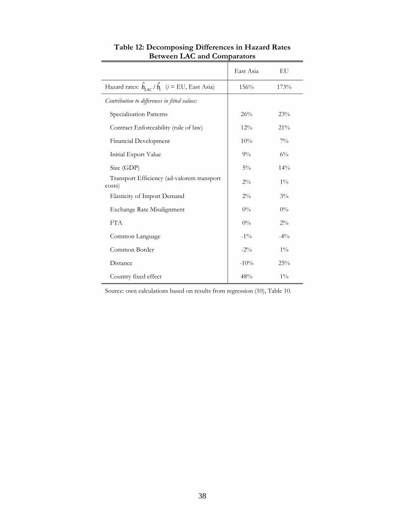
38

Table 12: Decomposing Differences in Hazard Rates Between LAC and Comparators

East Asia EU

Hazard rates: iLAC hh ˆ/ˆ (i = EU, East Asia) 156% 173%

Contribution to differences in fitted values:

Specialization Patterns 26% 23%

Contract Enforceability (rule of law) 12% 21%

Financial Development 10% 7%

Initial Export Value 9% 6%

Size (GDP) 5% 14%

Transport Efficiency (ad-valorem transport costs)

2% 1%

Elasticity of Import Demand 2% 3%

Exchange Rate Misalignment 0% 0%

FTA 0% 2%

Common Language -1% -4%

Common Border -2% 1%

Distance -10% 25%

Country fixed effect 48% 1%

Source: own calculations based on results from regression (10), Table 10.

39

Figure 1: Export Duration by Regions Figure 2: Export Duration by Regions Kaplan-Meier Survival Estimates using 6-digit HS Level Data

Kaplan-Meier Survival Estimates

0.0

00

.25

0.5

00

.75

1.0

0

Pro

babi

lity

of s

urv

iva

l

0 5 10 15

Time

US EU-15East Asia LAC

0.0

00

.25

0.5

00

.75

1.0

0

Pro

babi

lity

of s

urv

iva

l

0 5 10 15

Time

US EUEast Asia LAC

Figure 3: Export Duration by LAC Figure 4: Export Duration by Sub- regions Rauch’s Product Classification

Kaplan-Meier Survival Estimates Kaplan-Meier Survival Estimates

0.0

00

.25

0.5

00

.75

1.0

0

Pro

babi

lity

of s

urv

iva

l

0 5 10 15

Time

East Asia SouthAndean CentralCaribbean

0.0

00

.25

0.5

00

.75

1.0

0

Pro

babi

lity

of s

urv

iva

l

0 5 10 15

Time

Homogeneous ReferenceDifferentiated

40

Figure 5.1: Argentina Figure 5.2: Barbados

05

000

100

001

5000

MM

US

$

1970 1980 1990 2000 2010

Year

Actual Counterfactual

01

002

003

004

00

MM

US

$

1970 1980 1990 2000 2010

Year

Actual Counterfactual

Figure 5.3: Bolivia Figure 5.4: Brazil

05

001

000

150

0

MM

US

$

1970 1980 1990 2000 2010

Year

Actual Counterfactual

02

0000

400

006

0000

800

00

MM

US

$

1970 1980 1990 2000 2010

Year

Actual Counterfactual

Figure 5.5: Chile Figure 5.6: Colombia

05

000

100

001

5000

200

00

MM

US

$

1970 1980 1990 2000 2010

Year

Actual Counterfactual

02

000

400

06

000

800

0

MM

US

$

1970 1980 1990 2000 2010

Year

Actual Counterfactual

41

Figure 5.7: Costa Rica Figure 5.8: Ecuador

01

000

200

03

000

400

05

000

MM

US

$

1970 1980 1990 2000 2010

Year

Actual Counterfactual

05

001

000

150

0

MM

US

$

1970 1980 1990 2000 2010

Year

Actual Counterfactual

Figure 5.9: Guatemala Figure 5.10: Honduras

01

000

200

03

000

MM

US

$

1970 1980 1990 2000 2010

Year

Actual Counterfactual

02

004

006

00

MM

US

$

1970 1980 1990 2000 2010

Year

Actual Counterfactual

Figure 5.11: Jamaica Figure 5.l2: Mexico

500

100

01

500

200

02

500

MM

US

$

1970 1980 1990 2000 2010

Year

Actual Counterfactual

05

0000

100

000

150

000

200

000

MM

US

$

1970 1980 1990 2000 2010

Year

Actual Counterfactual

42

Figure 5.13: Nicaragua Figure 5.14: Panama

01

002

003

004

00

MM

US

$

1970 1980 1990 2000 2010

Year

Actual Counterfactual

01

002

003

00

MM

US

$

1970 1980 1990 2000 2010

Year

Actual Counterfactual

Figure 5.15: Peru Figure 5.16: Paraguay

02

000

400

06

000

MM

US

$

1970 1980 1990 2000 2010

Year

Actual Counterfactual

01

002

003

004

00

MM

US

$

1970 1980 1990 2000 2010

Year

Actual Counterfactual

Figure 5.17: El Salvador Figure 5.18: Trinidad and Tobago

02

004

006

008

001

000

MM

US

$

1970 1980 1990 2000 2010

Year

Actual Counterfactual

01

000

200

03

000

MM

US

$

1970 1980 1990 2000 2010

Year

Actual Counterfactual

43

Figure 5.19: Uruguay Figure 5.20: Venezuela

05

001

000

150

0

MM

US

$

1970 1980 1990 2000 2010

Year

Actual Counterfactual

02

000

400

06

000

800

01

0000

MM

US

$

1970 1980 1990 2000 2010

Year

Actual Counterfactual

Figure 6: Increase in the Annual Growth Rate of Exports Assuming East Asian Survival Rates

0.0%

0.5%

1.0%

1.5%

2.0%

2.5%

3.0%

3.5%

4.0%

4.5%

Pan

ama

N

icara

gua

Bol

ivia

Bar

bados

Ja

maic

a

H

ondura

s

Par

aguay

Uru

guay

Ven

ezuela

Ecu

ador

Per

u

Chile

Cos

ta R

ica

T&

T

Arg

entin

a

Col

ombia

El S

alvad

or

Guat

emala

Bra

zil

M

exico