Appendix A: The Model

Thomas F. Rutherford

University of Colorado at Boulder

David G. Tarr

The World Bank

June 2004

1 Algebraic Formulation

The model is based on the common features of general equilibrium models, including

market clearance and income balance. Optimizing choices by firms imply zero pure

profit with individuals firms equating marginal revenue and marginal cost. Final

demand arises from a representative household who earns income from the sale

of primary factors (capital, skilled and unskilled labor). The model includes one

additional primary factor, imported-specialized inputs to FDI service firms.

The government levies direct and indirect taxes and purchases a vector of goods

and services. In this section we outline the key features of the model in terms of the

objectives and constraints facing various agents.

1.1 Consumer Behavior

Private consumption in the model arises from budget-constrained utility maximiza-

tion. Preferences are represented as a Cobb-Douglas aggregate of goods and services:

U(C) =Xi

θi log(ci) (1)

1

in which associated demand functions are defined in terms of goods prices pi, con-

sumption tax rates and aggregate income, M :

ci =θiM

pi(1 + tCi )(2)

Income is defined in terms of sources of factor income: 1

M =X

w L + rKK +Xi

rSi ki +Xi,f

rRi,f Rif − TLS (3)

The right side of the budget constraint includes wage income, capital earnings

and net tax liabilities.

There are two types of sector-specific capital in the model. The first, correspond-

ing to termP

i rSi ki, represents resource rents associated with energy producing sec-

tors (gas, coal and oil). The existence of these fixed factors of production implies

that the associated production sectors exhibit diminishing marginal productivity in

terms of other inputs, and changes in the marginal return to these factors determines

the supply response of resrouce sectors to changes in output prices.

The second type of specific capital rents are represented by the termP

i,f rRi,f Rif .

This value accounts for rents which accrue to domestic and multinational firms as

a result of entry and exit to the industry. The number of firms of a particular type

responds to changes in profitability. As firms enter an industry rents associated with

these specific factors increas. We interpret these inputs as scarce resources specific

to domestic or multinational firms.

The lump-sum tax term is determined endogenously to balance the government

budget and hold public output constant (see below).

1.2 Domestic Supply

Goods and services are produced for sale in the domestic and international markets.

A constant-elasticity-of-transformation (CET) function shows the transformation

1In the short-run version of the model we assume that labor is sector specific, inwhich case labor income,

Pw L , is replaced by

Pi, w

S,iL

Si, .

2

possibilities in a given period between domestic (Di) and export (Ei) sales for a

given composite output level (Yi). The shares of sales at home and abroad are

determined by relative prices given that firms produce the final good to maximize

profit subject to the CET constraint:

Yi = Yi

"θD

µDi

Di

¶ 1+ηη

+ (1− θD)

µEi

Ei

¶ 1+ηη

# η1+η

(4)

In this equation parameters are the base year output for the domestic and export

markets, respectively, and θD is the baseline value share of domestic sales in total

sales, and η is the elasticity of transformation.

Production is associated with a nested production function of materials inputs

ami, labor services L ,i , and capital (Ki).2 Given prices of intermediate goods and

labor, the aggregate production sector operates so to minimize the costs of producing

a given output subject to the constraint:

Yi = Yimin [ami, Fi (Bi(asi), V Ai(L ,i,Ki, ))] (5)

in which ami = (am1,i, am2,i, . . .) represents material inputs to sector i, while asi =

(as1,i, as2,i, . . .) stands for inputs of business services. Within this function service

inputs substitute for primary factors trhough the production function Fi, Bi char-acterizes an aggregation of business services, and V Ai represents a Cobb-Douglas

aggregate of capital, skilled and unskilled labor.

1.3 Differentiated Services

Business services produced within the domestic economy are produced by two types

of imperfectly competitive firms: domestic and multinational. There is a one to one

correspondence between firms and their differentiated service varieties. For clarity

of notation we will dispense with the sectoral index, j in this discussion and focus

on a representative aggregate of a specific business service, Z. This composite is

2For energy resource sectors, inputs of mobile capital are replaced by sector-specific capita, ki

3

formed as a constant-elasticity-of-substitution (CES) function of ZD (domestic) and

ZM (multinational) service varieties, each of which is in turn a CES function of the

individual varieties, zdi and zmi respectively.

Z = (ZDδ + ZM δ)1/δ

in which

ZD =

"ndXi=1

zdδdi

#1/δdand

ZM =

"nmXi=1

zmδmi

#1/δmwhere nd and nm are the number of domestic and imported service varieties, respec-

tively. The elasticities of substitution within product groups are: σf = 1/(1 − δf)

for f ∈ {d,m}. We require that δf is a number between 0 and 1, which implies thatthe elasticities of substitution within product groups exceed unity.

Domestic services ZD are produced using domestic factors of production, whereas

multinational services ZM are produced using both domestic and imported inputs.

Examples of these imported inputs for services produced by multinational firms in-

clude specialized technical expertise, advanced technology, management techniques

and marketing expertise. These represent a wide range of specialized inputs and

thereby capture a key difference between multinational and domestic production

structures. Outputs of representative firms, zdi and zmi, are produced under in-

creasing returns to scale with a fixed cost of entry and a constant variable cost.

Because costs involve both fixed and marginal compoenets, it is convenient to

express technologies for these differentiated goods by cost rather than production

functions. Let CD and CM be the (total) cost functions for producing individual

domestic and multinational varieties. We impose a symmetry assumption within

firm types, i.e., all multinational firms have identical cost structures, and all domestic

firms that operate have cost structures identical to other domestic firms. cd and

cm represent unit variable cost functions and fd and fm represent the fixed costs

functions for domestic and multinational varieties respectively. Cost functions for

4

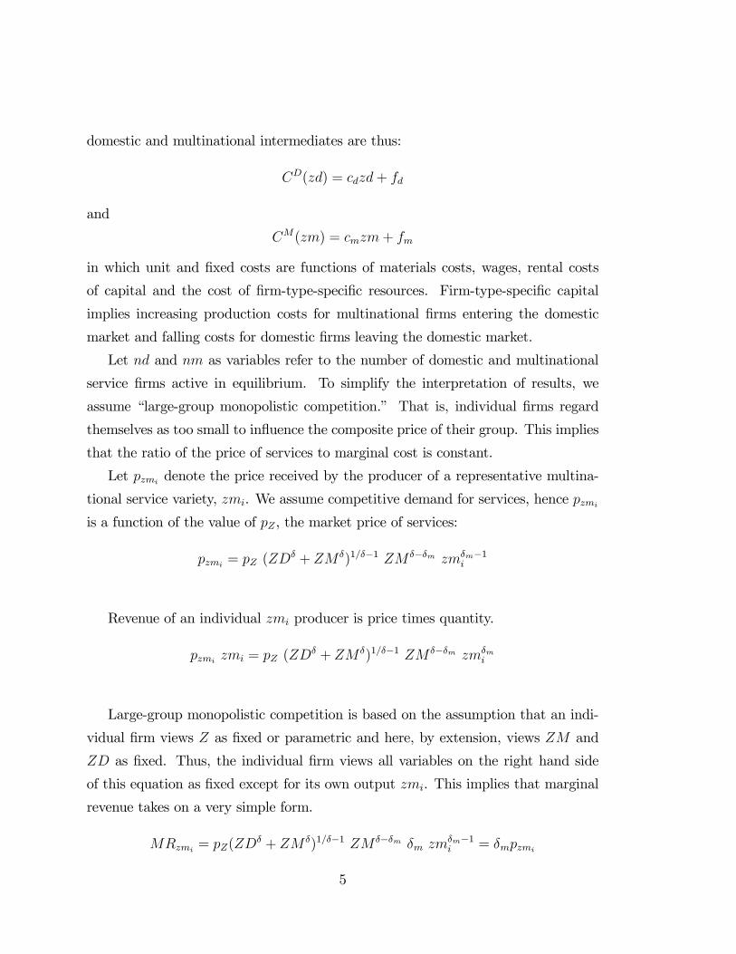
domestic and multinational intermediates are thus:

CD(zd) = cdzd+ fd

and

CM(zm) = cmzm+ fm

in which unit and fixed costs are functions of materials costs, wages, rental costs

of capital and the cost of firm-type-specific resources. Firm-type-specific capital

implies increasing production costs for multinational firms entering the domestic

market and falling costs for domestic firms leaving the domestic market.

Let nd and nm as variables refer to the number of domestic and multinational

service firms active in equilibrium. To simplify the interpretation of results, we

assume “large-group monopolistic competition.” That is, individual firms regard

themselves as too small to influence the composite price of their group. This implies

that the ratio of the price of services to marginal cost is constant.

Let pzmi denote the price received by the producer of a representative multina-

tional service variety, zmi. We assume competitive demand for services, hence pzmi

is a function of the value of pZ, the market price of services:

pzmi = pZ (ZDδ + ZM δ)1/δ−1 ZM δ−δm zmδm−1

i

Revenue of an individual zmi producer is price times quantity.

pzmi zmi = pZ (ZDδ + ZM δ)1/δ−1 ZM δ−δm zmδm

i

Large-group monopolistic competition is based on the assumption that an indi-

vidual firm views Z as fixed or parametric and here, by extension, views ZM and

ZD as fixed. Thus, the individual firm views all variables on the right hand side

of this equation as fixed except for its own output zmi. This implies that marginal

revenue takes on a very simple form.

MRzmi = pZ(ZDδ + ZM δ)1/δ−1 ZM δ−δm δm zmδm−1

i = δmpzmi

5

Setting marginal revenue equal to marginal cost implies that the ratio of price

to marginal cost is simply 1/δm. We have assumed that all multinational varieties

have an identical cost structure and the demand for all multinational varieties is

identical. These “symmetry” assumptions imply that the output and price of all

multinational firms that operate will be identical. We can thus write zmi = zm and

pzmi = pzm for all i. Similar conclusions follow for domestic firms.

Equilibrium for a symmetric group of service firms (zm or zd) is found as the

solution to two equations and two unknowns. One equation is the individual firm’s

optimization condition, marginal revenue equals marginal cost. A second condition,

arising from the free-entry condition, is that price equals average cost. This condition

determines the number of firms in equilibrium.

As noted above, the crucial distinction between domestic and international firms

follows from the technology through which services are produced. Domestic service

providers invoke costs which are largely based on primary factors, including labor,

capital (both mobile and firm-specific), and intermediate goods. Hence, we have:

cd = cd(w , rK, rRd , p)

Firms which provide services under FDI incur many of the same costs as domestic

firms, with the addition of an additional specialed input, pV :

cm = cm(w , rK , rRm, p, p

V )

pV represents the cost of specialized imported inputs and depends on the inter-

national price of these items. The domestic price of V is thus defined as the product

of the international price of V and the price of foreign exchange:

pV = pV ρ

6

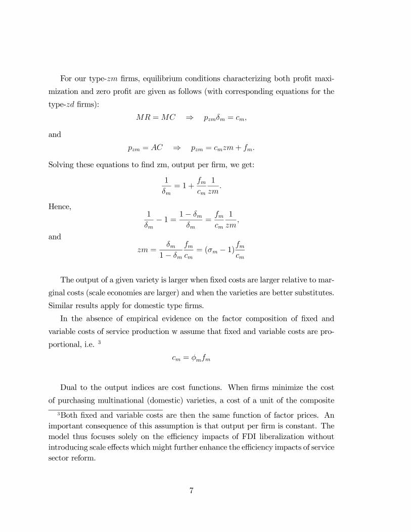
For our type-zm firms, equilibrium conditions characterizing both profit maxi-

mization and zero profit are given as follows (with corresponding equations for the

type-zd firms):

MR =MC ⇒ pzmδm = cm,

and

pzm = AC ⇒ pzm = cmzm+ fm.

Solving these equations to find zm, output per firm, we get:

1

δm= 1 +

fmcm

1

zm.

Hence,1

δm− 1 = 1− δm

δm=

fmcm

1

zm,

and

zm =δm

1− δm

fmcm= (σm − 1)

fmcm

The output of a given variety is larger when fixed costs are larger relative to mar-

ginal costs (scale economies are larger) and when the varieties are better substitutes.

Similar results apply for domestic type firms.

In the absence of empirical evidence on the factor composition of fixed and

variable costs of service production w assume that fixed and variable costs are pro-

portional, i.e. 3

cm = φmfm

Dual to the output indices are cost functions. When firms minimize the cost

of purchasing multinational (domestic) varieties, a cost of a unit of the composite

3Both fixed and variable costs are then the same function of factor prices. Animportant consequence of this assumption is that output per firm is constant. Themodel thus focuses solely on the efficiency impacts of FDI liberalization withoutintroducing scale effects which might further enhance the efficiency impacts of servicesector reform.

7

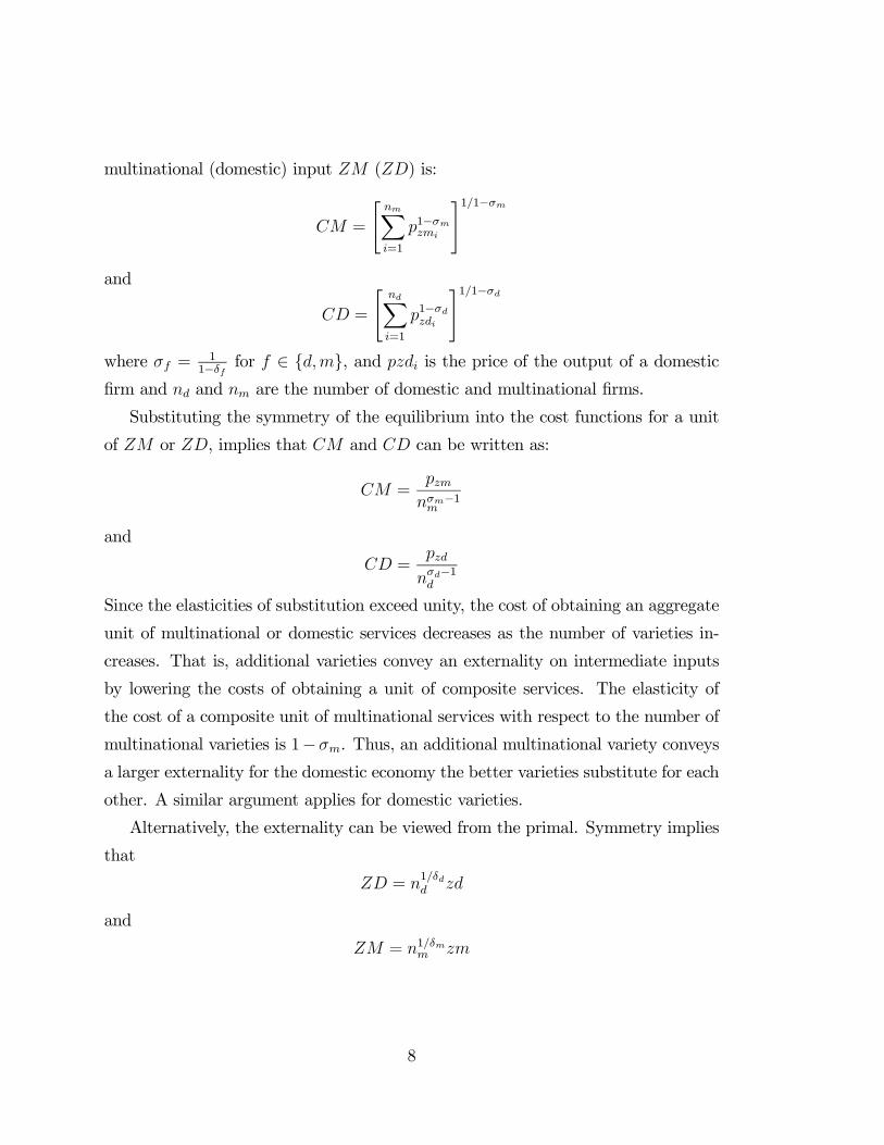
multinational (domestic) input ZM (ZD) is:

CM =

"nmXi=1

p1−σmzmi

#1/1−σmand

CD =

"ndXi=1

p1−σdzdi

#1/1−σdwhere σf = 1

1−δf for f ∈ {d,m}, and pzdi is the price of the output of a domestic

firm and nd and nm are the number of domestic and multinational firms.

Substituting the symmetry of the equilibrium into the cost functions for a unit

of ZM or ZD, implies that CM and CD can be written as:

CM =pzmnσm−1m

and

CD =pzd

nσd−1d

Since the elasticities of substitution exceed unity, the cost of obtaining an aggregate

unit of multinational or domestic services decreases as the number of varieties in-

creases. That is, additional varieties convey an externality on intermediate inputs

by lowering the costs of obtaining a unit of composite services. The elasticity of

the cost of a composite unit of multinational services with respect to the number of

multinational varieties is 1−σm. Thus, an additional multinational variety conveys

a larger externality for the domestic economy the better varieties substitute for each

other. A similar argument applies for domestic varieties.

Alternatively, the externality can be viewed from the primal. Symmetry implies

that

ZD = n1/δdd zd

and

ZM = n1/δmm zm

8

The cost of purchasing the output of domestic firms is nd × zd × pzd, which

increases in proportion to the number of fimrs. But, since δd < 1, the effective

supply to the firm increases more than proportionately with the number of firms.

Note in the special case of firm-level product differentiation in which δ = δd = δm

and zm = zd, Z can be written as:

Z = (nd + nm)1/δz

with z = zm = zd. In this case domestic and imported firms, while differentiated,

are perfect substitutes at the margin.

1.4 Differentiated Goods

Goods produced subject to increasing returns to scale are characterized as differen-

tiated products of domestic and foreign firms. For simplicity, each firm is assumed

to produce a single variety. Aggregate supply in a given sector is represented by a

composite of domestic and imported goods:

A =

ÃnX

j=1

xρj

!1/ρ

=

ÃnDXj=1

(xDj )ρ +

nMXj=1

(xMj )ρ

!1/ρ=

³n1−ρD (XD

j )ρ + n1−ρM (XM

j )ρ´1/ρ

(6)

In the final expression is output of a representative type k firm, and is resource

inputs at marginal cost of all type k firms.

Holding total output constant, effective supply of either domestic or foreign vari-

eties of commodity i increases with (nki )1−ρρ , which is the “variety effect multiplier.”

The multiplier increases with nki and increases as the elasticity of substitution de-

creases toward 1.

The supply of good i equals aggregate demand, the sum of intermediate demand,

consumer demand, investment demand, government demand and the demand for

9

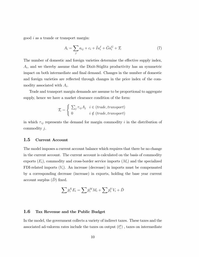
good i as a trande or transport margin:

Ai =Xj

aij + ci + IaIi + GaGi + Ti (7)

The number of domestic and foreign varieties determine the effective supply index,

Ai, and we thereby assume that the Dixit-Stiglitz productivity has an symmetric

impact on both intermediate and final demand. Changes in the number of domestic

and foreign varieties are reflected through changes in the price index of the com-

modity associated with Ai.

Trade and transport margin demands are assume to be proportional to aggregate

supply, hence we have a market clearance condition of the form:

Ti =( P

j τ ijAj i ∈ (trade, transport)0 i /∈ (trade, transport)

in which τ ij represents the demand for margin commodity i in the distribution of

commodity j.

1.5 Current Account

The model imposes a current account balance which requires that there be no change

in the current account. The current account is calculated on the basis of commodity

exports (Ei), commodity and cross-border service imports (Mi) and the specialized

FDI-related imports (Vi). An increase (decrease) in imports must be compensated

by a corresponding decrease (increase) in exports, holding the base year current

account surplus (D) fixed.XpXi Ei =

XpMi Mi +

XpVi Vi + D

1.6 Tax Revenue and the Public Budget

In the model, the government collects a variety of indirect taxes. These taxes and the

associated ad-valorem rates include the taxes on output (tyi ) , taxes on intermediate

10

inputs (taij) , tariffs (tMi ), taxes on public demand (t

Gi ), taxes on investment demand

(tIi ) , taxes on exports (tXir), and taxes on consumption (t

Ci ). The government budget

constraint is then:

pGG = TY + Ta + TM + TG + TI + TX + TC + TLS

in which Tk represents revenue from tax instrument k, and TLS represents direct

(lump-sum) taxes. The model features a constant level of public provision, which is

achieved through adjustment of the level of lump sum tax.

11

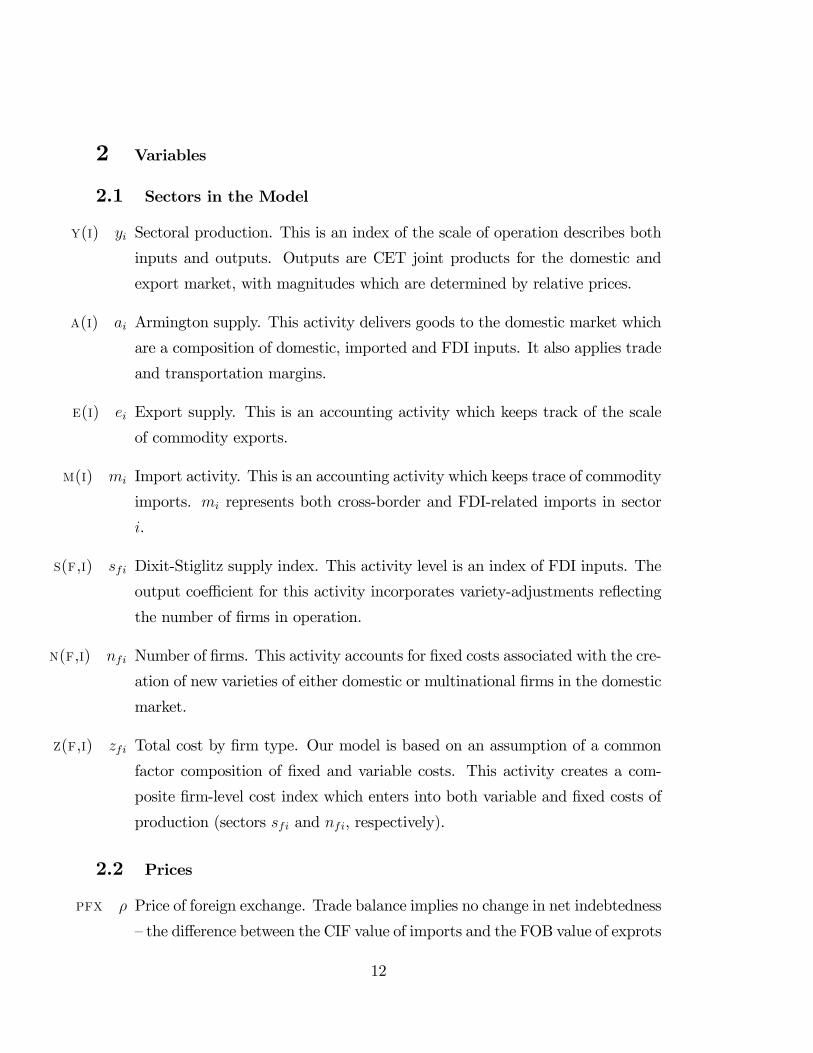
2 Variables

2.1 Sectors in the Model

y(i) yi Sectoral production. This is an index of the scale of operation describes both

inputs and outputs. Outputs are CET joint products for the domestic and

export market, with magnitudes which are determined by relative prices.

a(i) ai Armington supply. This activity delivers goods to the domestic market which

are a composition of domestic, imported and FDI inputs. It also applies trade

and transportation margins.

e(i) ei Export supply. This is an accounting activity which keeps track of the scale

of commodity exports.

m(i) mi Import activity. This is an accounting activity which keeps trace of commodity

imports. mi represents both cross-border and FDI-related imports in sector

i.

s(f,i) sfi Dixit-Stiglitz supply index. This activity level is an index of FDI inputs. The

output coefficient for this activity incorporates variety-adjustments reflecting

the number of firms in operation.

n(f,i) nfi Number of firms. This activity accounts for fixed costs associated with the cre-

ation of new varieties of either domestic or multinational firms in the domestic

market.

z(f,i) zfi Total cost by firm type. Our model is based on an assumption of a common

factor composition of fixed and variable costs. This activity creates a com-

posite firm-level cost index which enters into both variable and fixed costs of

production (sectors sfi and nfi, respectively).

2.2 Prices

pfx ρ Price of foreign exchange. Trade balance implies no change in net indebtedness

— the difference between the CIF value of imports and the FOB value of exprots

12

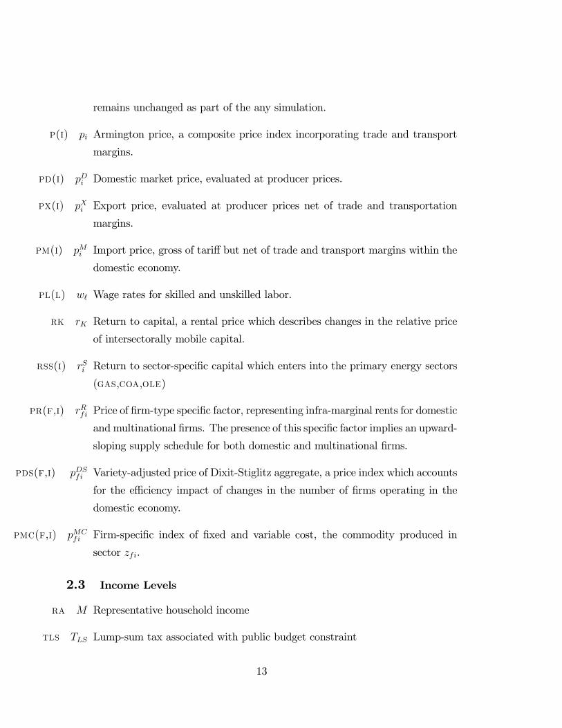
remains unchanged as part of the any simulation.

p(i) pi Armington price, a composite price index incorporating trade and transport

margins.

pd(i) pDi Domestic market price, evaluated at producer prices.

px(i) pXi Export price, evaluated at producer prices net of trade and transportation

margins.

pm(i) pMi Import price, gross of tariff but net of trade and transport margins within the

domestic economy.

pl(l) w Wage rates for skilled and unskilled labor.

rk rK Return to capital, a rental price which describes changes in the relative price

of intersectorally mobile capital.

rss(i) rSi Return to sector-specific capital which enters into the primary energy sectors

(gas,coa,ole)

pr(f,i) rRfi Price of firm-type specific factor, representing infra-marginal rents for domestic

and multinational firms. The presence of this specific factor implies an upward-

sloping supply schedule for both domestic and multinational firms.

pds(f,i) pDSfi Variety-adjusted price of Dixit-Stiglitz aggregate, a price index which accounts

for the efficiency impact of changes in the number of firms operating in the

domestic economy.

pmc(f,i) pMCfi Firm-specific index of fixed and variable cost, the commodity produced in

sector zfi.

2.3 Income Levels

ra M Representative household income

tls TLS Lump-sum tax associated with public budget constraint

13

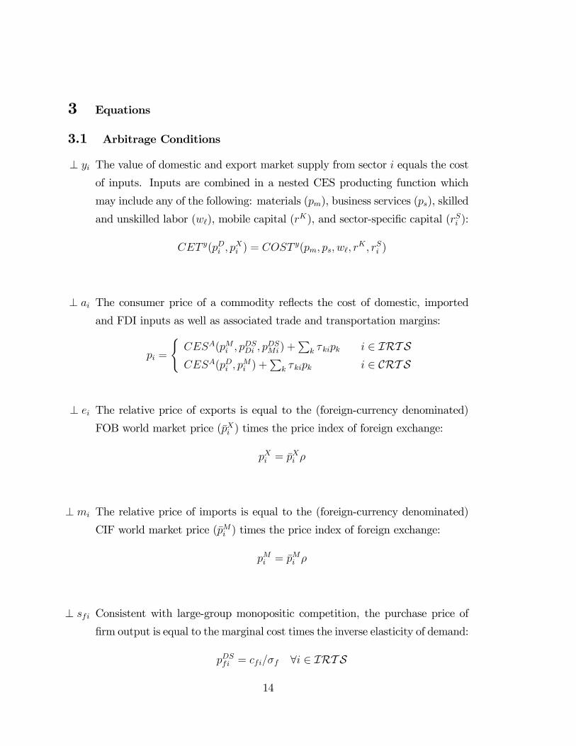
3 Equations

3.1 Arbitrage Conditions

⊥ yi The value of domestic and export market supply from sector i equals the cost

of inputs. Inputs are combined in a nested CES producting function which

may include any of the following: materials (pm), business services (ps), skilled

and unskilled labor (w ), mobile capital (rK), and sector-specific capital (rSi ):

CET y(pDi , pXi ) = COST y(pm, ps, w , rK , rSi )

⊥ ai The consumer price of a commodity reflects the cost of domestic, imported

and FDI inputs as well as associated trade and transportation margins:

pi =

(CESA(pMi , pDS

Di , pDSMi ) +

Pk τkipk i ∈ IRT S

CESA(pDi , pMi ) +

Pk τkipk i ∈ CRT S

⊥ ei The relative price of exports is equal to the (foreign-currency denominated)

FOB world market price (pXi ) times the price index of foreign exchange:

pXi = pXi ρ

⊥ mi The relative price of imports is equal to the (foreign-currency denominated)

CIF world market price (pMi ) times the price index of foreign exchange:

pMi = pMi ρ

⊥ sfi Consistent with large-group monopositic competition, the purchase price of

firm output is equal to the marginal cost times the inverse elasticity of demand:

pDSfi = cfi/σf ∀i ∈ IRT S

14

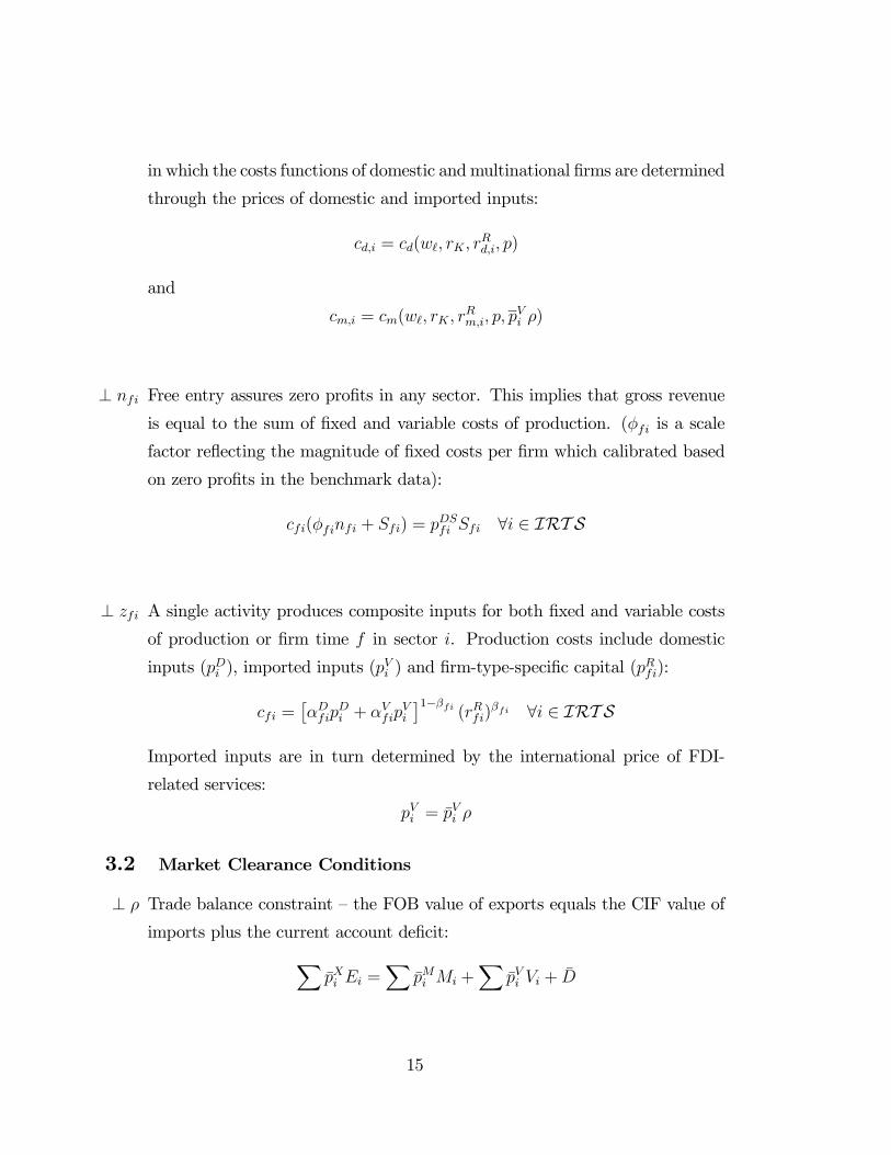
in which the costs functions of domestic and multinational firms are determined

through the prices of domestic and imported inputs:

cd,i = cd(w , rK, rRd,i, p)

and

cm,i = cm(w , rK, rRm,i, p, p

Vi ρ)

⊥ nfi Free entry assures zero profits in any sector. This implies that gross revenue

is equal to the sum of fixed and variable costs of production. (φfi is a scale

factor reflecting the magnitude of fixed costs per firm which calibrated based

on zero profits in the benchmark data):

cfi(φfinfi + Sfi) = pDSfi Sfi ∀i ∈ IRT S

⊥ zfi A single activity produces composite inputs for both fixed and variable costs

of production or firm time f in sector i. Production costs include domestic

inputs (pDi ), imported inputs (pVi ) and firm-type-specific capital (p

Rfi):

cfi =£αDfip

Di + αV

fipVi

¤1−βfi (rRfi)βfi ∀i ∈ IRT SImported inputs are in turn determined by the international price of FDI-

related services:

pVi = pVi ρ

3.2 Market Clearance Conditions

⊥ ρ Trade balance constraint — the FOB value of exports equals the CIF value of

imports plus the current account deficit:XpXi Ei =

XpMi Mi +

XpVi Vi + D

15

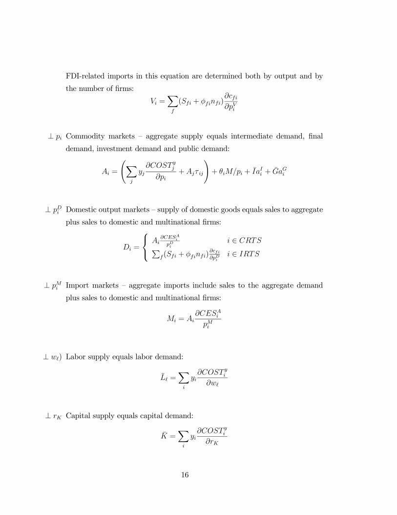
FDI-related imports in this equation are determined both by output and by

the number of firms:

Vi =Xf

(Sfi + φfinfi)∂cfi∂pVi

⊥ pi Commodity markets — aggregate supply equals intermediate demand, final

demand, investment demand and public demand:

Ai =

ÃXj

yj∂COST y

j

∂pi+Ajτ ij

!+ θiM/pi + IaIi + GaGi

⊥ pDi Domestic output markets — supply of domestic goods equals sales to aggregate

plus sales to domestic and multinational firms:

Di =

Ai∂CESAi

pDii ∈ CRTSP

f(Sfi + φfinfi)∂cfi∂pDi

i ∈ IRTS

⊥ pMi Import markets — aggregate imports include sales to the aggregate demand

plus sales to domestic and multinational firms:

Mi = Ai∂CESA

i

pMi

⊥ w ) Labor supply equals labor demand:

L =Xi

yi∂COST y

i

∂w

⊥ rK Capital supply equals capital demand:

K =Xi

yi∂COST y

i

∂rK

16

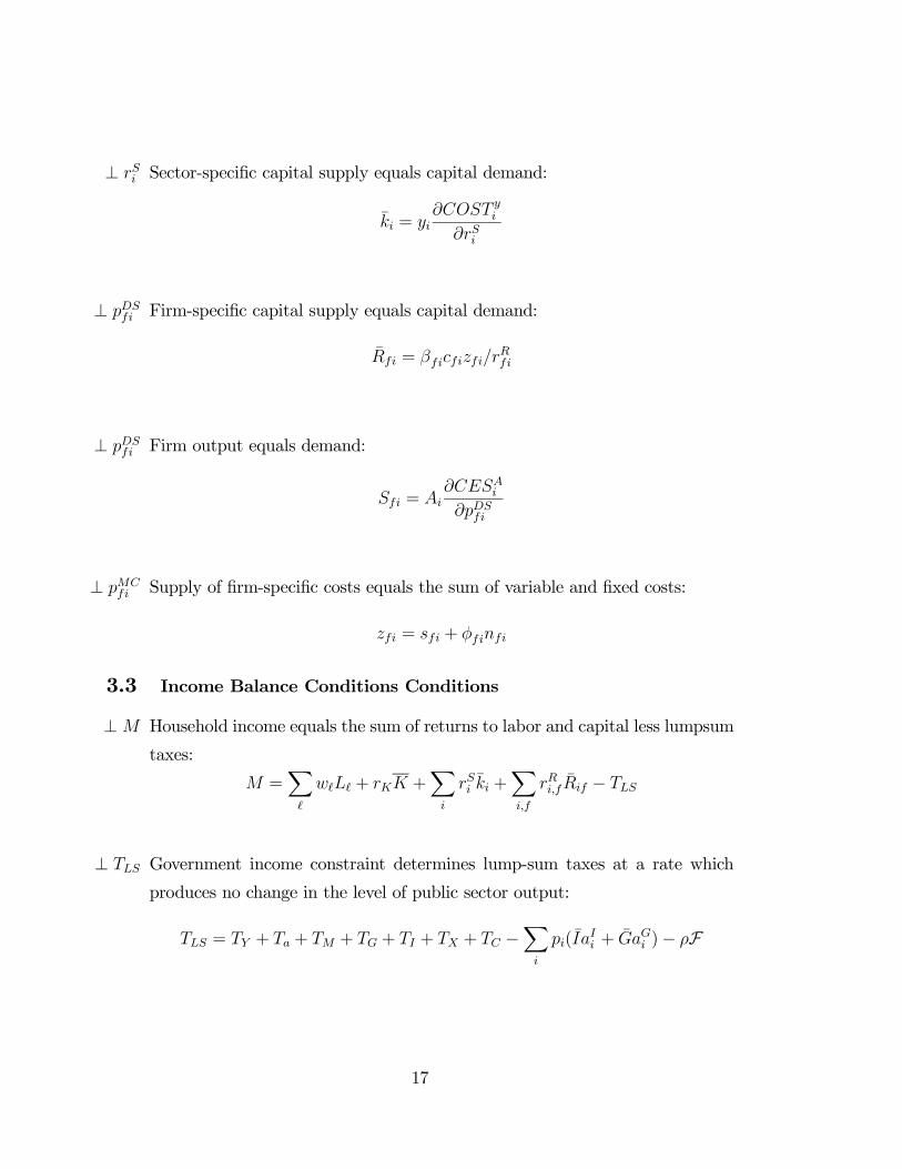
⊥ rSi Sector-specific capital supply equals capital demand:

ki = yi∂COST y

i

∂rSi

⊥ pDSfi Firm-specific capital supply equals capital demand:

Rfi = βficfizfi/rRfi

⊥ pDSfi Firm output equals demand:

Sfi = Ai∂CESA

i

∂pDSfi

⊥ pMCfi Supply of firm-specific costs equals the sum of variable and fixed costs:

zfi = sfi + φfinfi

3.3 Income Balance Conditions Conditions

⊥M Household income equals the sum of returns to labor and capital less lumpsum

taxes:

M =X

w L + rKK +Xi

rSi ki +Xi,f

rRi,f Rif − TLS

⊥ TLS Government income constraint determines lump-sum taxes at a rate which

produces no change in the level of public sector output:

TLS = TY + Ta + TM + TG + TI + TX + TC −Xi

pi(IaIi + GaGi )− ρF

17

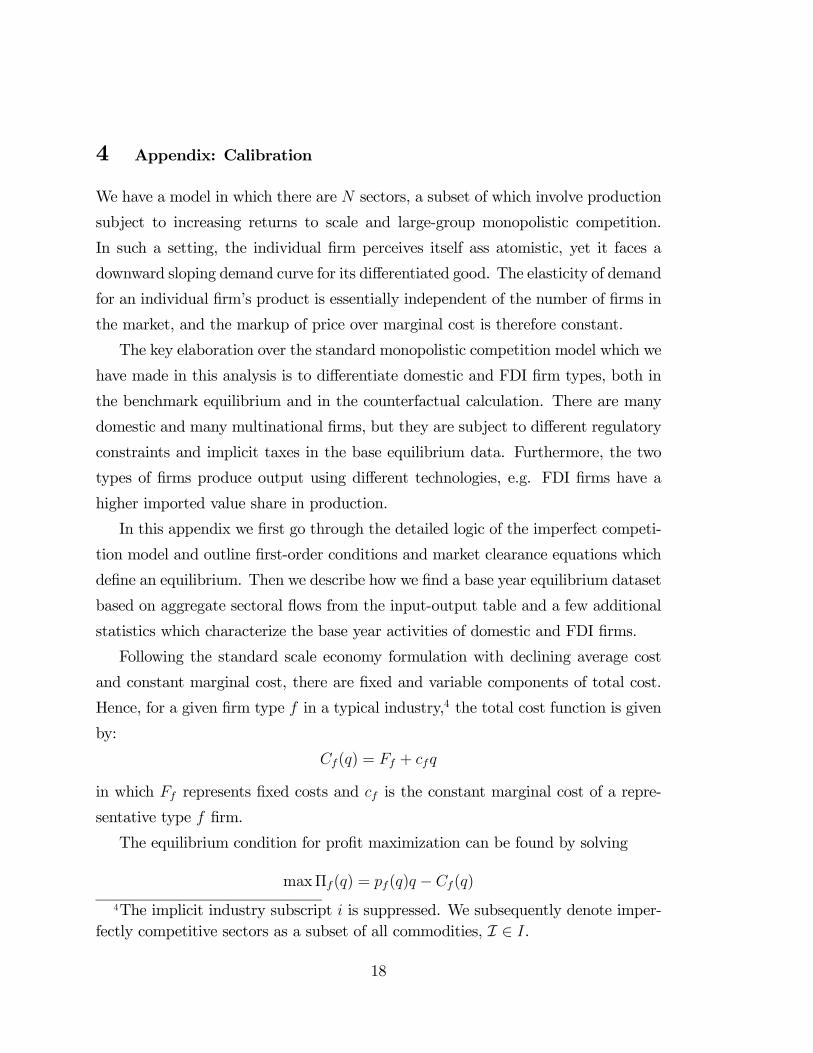
4 Appendix: Calibration

We have a model in which there are N sectors, a subset of which involve production

subject to increasing returns to scale and large-group monopolistic competition.

In such a setting, the individual firm perceives itself ass atomistic, yet it faces a

downward sloping demand curve for its differentiated good. The elasticity of demand

for an individual firm’s product is essentially independent of the number of firms in

the market, and the markup of price over marginal cost is therefore constant.

The key elaboration over the standard monopolistic competition model which we

have made in this analysis is to differentiate domestic and FDI firm types, both in

the benchmark equilibrium and in the counterfactual calculation. There are many

domestic and many multinational firms, but they are subject to different regulatory

constraints and implicit taxes in the base equilibrium data. Furthermore, the two

types of firms produce output using different technologies, e.g. FDI firms have a

higher imported value share in production.

In this appendix we first go through the detailed logic of the imperfect competi-

tion model and outline first-order conditions and market clearance equations which

define an equilibrium. Then we describe how we find a base year equilibrium dataset

based on aggregate sectoral flows from the input-output table and a few additional

statistics which characterize the base year activities of domestic and FDI firms.

Following the standard scale economy formulation with declining average cost

and constant marginal cost, there are fixed and variable components of total cost.

Hence, for a given firm type f in a typical industry,4 the total cost function is given

by:

Cf(q) = Ff + cfq

in which Ff represents fixed costs and cf is the constant marginal cost of a repre-

sentative type f firm.

The equilibrium condition for profit maximization can be found by solving

maxΠf(q) = pf(q)q − Cf(q)

4The implicit industry subscript i is suppressed. We subsequently denote imper-fectly competitive sectors as a subset of all commodities, I ∈ I.

18

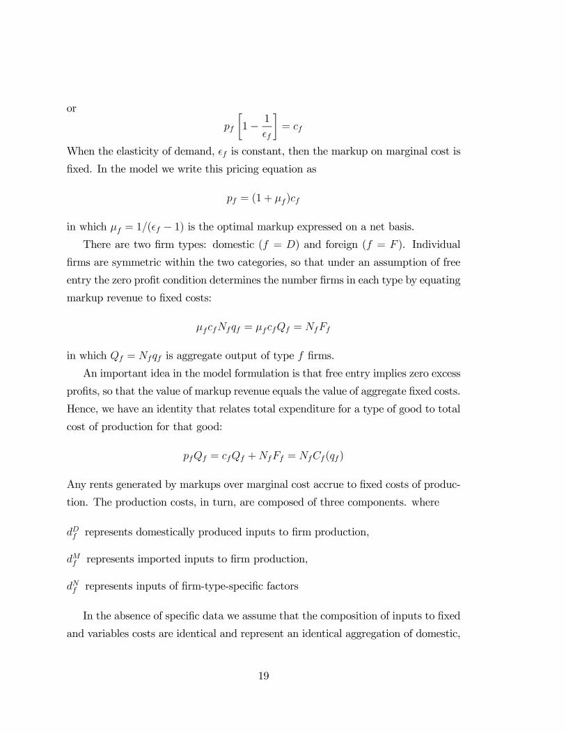
or

pf

·1− 1

f

¸= cf

When the elasticity of demand, f is constant, then the markup on marginal cost is

fixed. In the model we write this pricing equation as

pf = (1 + µf)cf

in which µf = 1/( f − 1) is the optimal markup expressed on a net basis.There are two firm types: domestic (f = D) and foreign (f = F ). Individual

firms are symmetric within the two categories, so that under an assumption of free

entry the zero profit condition determines the number firms in each type by equating

markup revenue to fixed costs:

µfcfNfqf = µfcfQf = NfFf

in which Qf = Nfqf is aggregate output of type f firms.

An important idea in the model formulation is that free entry implies zero excess

profits, so that the value of markup revenue equals the value of aggregate fixed costs.

Hence, we have an identity that relates total expenditure for a type of good to total

cost of production for that good:

pfQf = cfQf +NfFf = NfCf(qf)

Any rents generated by markups over marginal cost accrue to fixed costs of produc-

tion. The production costs, in turn, are composed of three components. where

dDf represents domestically produced inputs to firm production,

dMf represents imported inputs to firm production,

dNf represents inputs of firm-type-specific factors

In the absence of specific data we assume that the composition of inputs to fixed

and variables costs are identical and represent an identical aggregation of domestic,

19

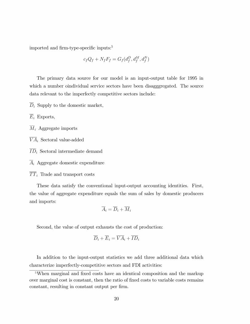
imported and firm-type-specific inputs:5

cfQf +NfFf = Gf(dDf , d

Mf , dNf )

The primary data source for our model is an input-output table for 1995 in

which a number oindividual service sectors have been disagggregated. The source

data relevant to the imperfectly competitive sectors include:

Di Supply to the domestic market,

Ei Exports,

M i Aggregate imports

V Ai Sectoral value-added

IDi Sectoral intermediate demand

Ai Aggregate domestic expenditure

TT i Trade and transport costs

These data satisfy the conventional input-output accounting identities. First,

the value of aggregate expenditure equals the sum of sales by domestic producers

and imports:

Ai = Di +M i

Second, the value of output exhausts the cost of production:

Di +Ei = V Ai + IDi

In addition to the input-output statistics we add three additional data which

characterize imperfectly-competitive sectors and FDI activities:5When marginal and fixed costs have an identical composition and the markup

over marginal cost is constant, then the ratio of fixed costs to variable costs remainsconstant, resulting in constant output per firm.

20

θFDIi Fraction of base year output in sector i which is supply by FDI firms.

θMf,i Share of production inputs for type f firms which are imported.

ηfi Elasticity of supply of type f firms in sector i with respect to the rate of return.

τ fi Implicit tax on firm type f in sector i, representing base year barriers to FDI.

The calibration procedure infers a set of benchmark equilibrium values so as

to retain benchmark consistency and applies additional assumptions regarding the

cost structure of firms and their market share. The values which are inferred by the

calibration process include:

Di Domestic supply to the domestic market,

Mi Aggregate imports

V Ai Sectoral value-added,

ADi “Ancillary demand” for domestic goods or services, representing domestic out-

put from sector i which is unrelated to the output of imperfectly competitive

firms.

AMi “Ancillary demand” for imported goods, representing imports of goods associ-

ated with sector i which is unrelated to the output of imperfectly competitive

firms.

MCf,i Aggregate marginal cost (Nfcf(qf)),

FCf,i Aggregate fixed costs (NfFf))

Firms engaged in foreign direct investment produce a specified fraction of output:

dSf,i = θFDIi

Xf 0

dSf 0,i i ∈ fdi (8)

The import share of cost for FDI firms is defined by θMf,i:

dMf,i = θMf,i(dMf,i + dDf,i) i ∈ fdi (9)

21

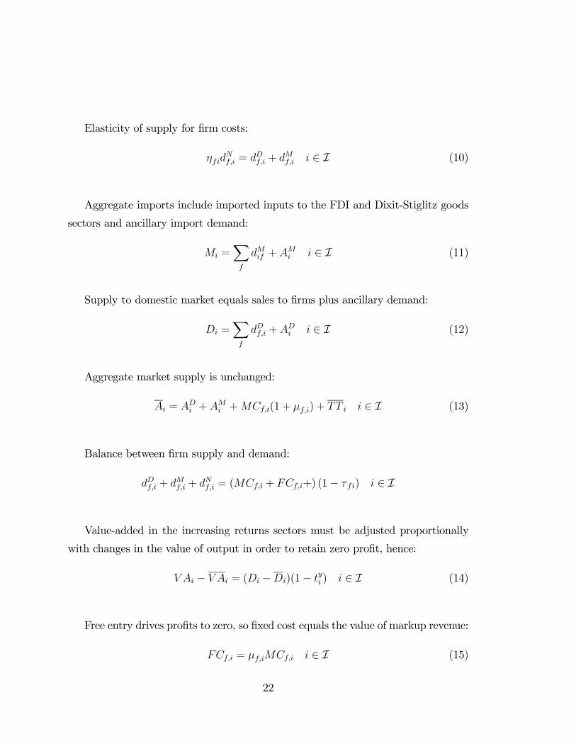
Elasticity of supply for firm costs:

ηfidNf,i = dDf,i + dMf,i i ∈ I (10)

Aggregate imports include imported inputs to the FDI and Dixit-Stiglitz goods

sectors and ancillary import demand:

Mi =Xf

dMif +AMi i ∈ I (11)

Supply to domestic market equals sales to firms plus ancillary demand:

Di =Xf

dDf,i +ADi i ∈ I (12)

Aggregate market supply is unchanged:

Ai = ADi +AM

i +MCf,i(1 + µf,i) + TT i i ∈ I (13)

Balance between firm supply and demand:

dDf,i + dMf,i + dNf,i = (MCf,i + FCf,i+) (1− τ fi) i ∈ I

Value-added in the increasing returns sectors must be adjusted proportionally

with changes in the value of output in order to retain zero profit, hence:

V Ai − V Ai = (Di −Di)(1− tyi ) i ∈ I (14)

Free entry drives profits to zero, so fixed cost equals the value of markup revenue:

FCf,i = µf,iMCf,i i ∈ I (15)

22

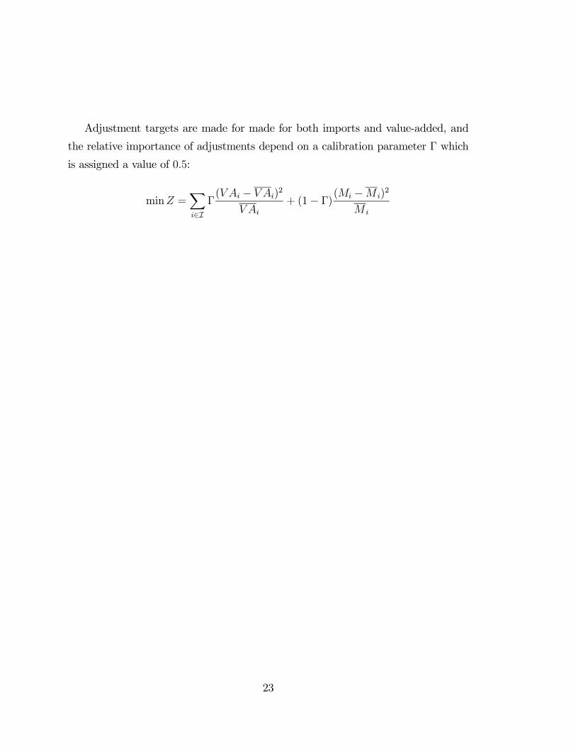
Adjustment targets are made for made for both imports and value-added, and

the relative importance of adjustments depend on a calibration parameter Γ which

is assigned a value of 0.5:

minZ =Xi∈I

Γ(V Ai − V Ai)

2

V Ai

+ (1− Γ)(Mi −M i)

2

M i

23