Embed Size (px)
Citation preview

Exploring effects of hydrodynamic flotation
variables on their respective metallurgical
responses through laboratory scaling up
Mohazzam Saeed
Master Programme in Georesources Engineering
2021
Luleå University of Technology
Department of Civil, Environmental and Natural Resources Engineering


Exploring effects of hydrodynamic flotation variables on their respective metallurgical responses through laboratory
scaling up
by:
Mohazzam Saeed
Division of Minerals and Metallurgical Engineering (MiMer) Department of Civil,
Environmental and Natural Resources Engineering Luleå University of Technology
Supervisor:
Vitalis Chipakwe
Examiner:
Saeed Chehreh Chelgani
Luleå, Sweden
2021


i
Abstract
To meet the increasing demand for raw materials, higher throughput of mineral separation
through froth flotation is becoming important. This higher throughput can be achieved by
increasing the size of flotation equipment termed scaling up. Flotation performance is greatly
affected by the size of flotation machines and remains an important research area to correlate
flotation behavior between small and larger flotation machines. The Outotec GTK LabCell®,
a mechanical flotation machine, has been used as a benchmark for many industrial pre-
feasibility studies around the world for the past decade. This study deals with the scale-up
assessment in terms of flotation rate constant between 2 L and 7.5 L flotation cells of the
Outotec GTK LabCell®, machine. The design of these lab scale flotation machines is
comparable to other Outotec industrial scale flotation equipment considering rotor and
impeller design, and the main difference is in scale. The influence of the hydrodynamic
parameters on the flotation performance in both the cells was investigated by varying the
impeller tip speed and superficial gas velocity. Particle size distribution analysis indicated
concentrate product was finer at smaller cell size at all combinations of impeller tip speed and
superficial gas velocity. The results showed for both cells, mass and water recovery increased
with an increase in the impeller tip speed and superficial gas velocity until a certain value,
after which they decreased. Maximum mass and water recovery were achieved using an
impeller tip speed of 3.1 m/s and superficial gas velocity of 0.21 cm/s. Flotation kinetic
analysis indicated scaling up of flotation cells was possible at different impeller tip speed by
keeping the superficial gas velocity at 0.21 cm/s.
Keywords: Froth flotation; Scale-up; Impeller tip speed; superficial gas velocity;
ii
Contents 1 Introduction ..................................................................................................................... 7
1.1 Motivation ................................................................................................................. 8
1.2 Research questions ................................................................................................... 9
1.3 Aim and Objective .................................................................................................... 9
1.4 Thesis Outline ........................................................................................................... 9
2 Literature Survey .......................................................................................................... 11
2.1 Froth flotation theory ............................................................................................. 11
2.2 Flotation reagents ................................................................................................... 14
2.2.1 Collectors .......................................................................................................... 14
2.2.2 Frothers ............................................................................................................. 16
2.2.3 Regulators ........................................................................................................ 17
2.3 Flotation circuits ..................................................................................................... 18
2.4 Flotation equipment ............................................................................................... 19
2.4.1 Mechanical flotation machines ...................................................................... 20
2.4.2 Pneumatic flotation machines ....................................................................... 21
2.4.3 Laboratory flotation machines ...................................................................... 23
2.5 Scale-up of flotation process ................................................................................. 24
2.5.1 Economics of Up-scaling ................................................................................ 25
2.5.2 Kinetic scale-up ............................................................................................... 26
2.5.3 Machine design scale-up ................................................................................ 32
2.6 Impeller speed ........................................................................................................ 34
2.7 Airflow rate ............................................................................................................. 37
3 Materials and Methodology ....................................................................................... 39
3.1 Flotation equipment ............................................................................................... 40
3.2 Sample Preparation ................................................................................................ 42
3.2.1 Grinding and Sieving ..................................................................................... 42
3.3 Flotation reagents selection ................................................................................... 43
3.4 Flotation experiment .............................................................................................. 44
4 Results ............................................................................................................................. 47
4.1 Mass recovery analysis .......................................................................................... 47
4.2 Water recovery analysis ........................................................................................ 50
4.3 Flotation rate constant analysis ............................................................................ 54
4.4 Particle size distribution ........................................................................................ 56
4.5 Scale-up Assessment .............................................................................................. 58

iii
4.5.1 Water recovery analysis ................................................................................. 58
4.5.2 Mass recovery analysis ................................................................................... 60
4.5.3 Scale-up Assessment flotation rate constant ............................................... 62
5 Discussion and Conclusions ...................................................................................... 66
5.1 Influence of Impeller tip speed............................................................................. 66
5.2 Influence of Airflow rate ....................................................................................... 67
5.3 Conclusion ............................................................................................................... 67
6 EIT Chapter .................................................................................................................... 70
6.1 Recommendations for Future Work .................................................................... 70
6.2 SWOT Analysis ....................................................................................................... 71
7 References ...................................................................................................................... 72
List of Figures
Figure 1. Increase in the flotation tank volume over the last century (Mesa and Brito-Parada 2019). ............................................................................................................................ 8 Figure 2. Structure of the thesis. ......................................................................................... 10 Figure 3. Factors affecting flotation system (Kawatra 2011). .......................................... 12 Figure 4. Flotation principle illustration (Brezáni and Zeleňák 2011). .......................... 12 Figure 5. The contact angle between the mineral surface and air bubble (Nguyen 2013) ........................................................................................................................................ 13 Figure 6. Collector adsorption on the surface of the mineral (Potapova, 2011). .......... 14 Figure 7. Adsorption of the ionizing collector on the mineral water interface extracted from (Nguyen 2013). ........................................................................................... 15 Figure 8. Typical Classification of collector extracted from (Nguyen 2013) ................ 15 Figure 9. The action of frothers on the air bubble (Wills et al. 2006) ............................. 16 Figure 10. Basic flotation circuit, rougher, scavenger, and cleaner (Wills et al. 2006).19 Figure 11. Typical mechanical flotation machine assembly (Strand et al. 2012) .......... 20 Figure 12. Hydrodynamic zones in a mechanical flotation machine (Anon 2017) ...... 21 Figure 13. Column flotation machines (Han et al. 2014) ................................................. 23 Figure 14. Increase in the flotation tank volume over the past century. (Govender 2013b) ...................................................................................................................................... 25 Figure 15. Lifetime cost analysis of different flotation cells (Rinne and Peltola 2008) 26 Figure 16. Relationship of Impeller's Reynold number and Power number (Mesa and Brito-Parada 2019). ................................................................................................................ 33 Figure 17. Rotor, Stator assembly (Impeller) inside the flotation cell (Souza Pinto et al. 2018). .................................................................................................................................. 35 Figure 18. Flowsheet for the sample preparation and flotation experiments. ............. 39 Figure 19. Outotec GTK LabCell®. ..................................................................................... 41 Figure 20. Different dimensions of Outotec GTK LabCells®. ........................................ 41 Figure 21. Particle size distribution, available sample and flotation feed. ................... 42 Figure 22. Recoveries for collector type and concentrations. ......................................... 44 Figure 23. Concentrate mass recovery of 2 L flotation cell. ............................................ 48 Figure 24. Concentrate mass recovery of 7.5 L flotation cell. ......................................... 48 Figure 25.Box and whisker plot for noncumulative mass recovery 2 L flotation cell . 50

iv
Figure 26. Box and whisker plot for noncumulative mass recovery 7.5 L flotation cell.................................................................................................................................................. 50 Figure 27.Cumulative water recovery 2L flotation cell ................................................... 51 Figure 28.Cumulative water recovery 7.5 L flotation cell. .............................................. 52 Figure 29. Box plot for noncumulative water recovery 2L cell. ..................................... 53 Figure 30. Box plot for noncumulative water recovery 7.5L cell. .................................. 53 Figure 31. Particle size distribution in different flotation setups for 2 L flotation cells.................................................................................................................................................. 57 Figure 32.Particle size distribution in different flotation setups for 7.5 L flotation cell................................................................................................................................................... 58 Figure 33. Scaling up assessments for water recovery based on the different impeller tip speeds. ............................................................................................................................... 59 Figure 34. Scaling up assessment for water recovery based on different impeller tip speeds. .................................................................................................................................... 60 Figure 35. Cumulative mass recovery scale-up assessment under constant superficial gas velocity and different impeller tip speeds. ................................................................. 61 Figure 36. Scaling up assessment for mass recovery based on same impeller tip speed and different superficial gas velocities. ............................................................................. 62 Figure 37. Model fitting for flotation rate constants between two cells. ....................... 63 Figure 38. Counter plots for flotation rate constant for 2L flotation cell. ..................... 64 Figure 39. Counter plots for flotation rate constant for 7.5L flotation cell. .................. 64 Figure 40. Flotation rate constant at the superficial gas velocity of 0.21 cm/s. ........... 65
List of tables
Table 1. Typical frothers used in froth flotation (Nguyen 2013) .................................... 17 Table 2. A selection of flotation kinetic models. ............................................................... 28 Table 3. Dimensionless numbers for flotation cells (Malhotra 2009) ............................ 30 Table 4. Flotation conditions for flotation analysis. ......................................................... 40 Table 5. Manufacturer recommended machine parameters for the different scales ... 42 Table 6. Grinding specifications for the Ball mill and Rod mill. .................................... 43 Table 7. Hydrodynamic conditions for flotation experiments. ...................................... 46 Table 8. Summary table for concentrate mass and water recovery for both cells. ...... 48 Table 9. Flotation kinetic table for 2L cell. ......................................................................... 54 Table 10. Flotation kinetic table for 7.5 L cell. ................................................................... 55

v
Acknowledgments
To begin with, I would like to express my sincere gratitude to my supervisors Prof Dr
Saeed Chehreh Chelgani and Vitalis Chipakwe for their continuous support during
my Master's thesis studies. Their continuous guidance helped me throughout this
research, work and achieving this milestone in my life. I could not have imagined
having better advisors and mentors for my Master's studies. It has been a pleasure
working under your kind supervision.
I would like to take the opportunity to thank my colleague July Anna Bazar, with
whom I shared amazing memories working together in the same lab. My other fellows
of Emerald Moshin, Ali, Asim, Bethlehem, Milkias, Barbara, Bastein, and Michele for
their constructive discussions and helping me with different things during my studies
on different occasions. I would also like to extend my thanks to Emerald fellows,
Joseph, Raoul, Gulsha, Nikka, Leo, Ramzan, Shayan, Kianoosh, Kaye, Galm, Aliza,
Rania, and all other friends for their great company and support. Additionally, I
would like to thank my dear friend Mukthair Ahmed who was with me every moment
and kept me going through the way.
Last but not the least, I would like to thank my mother (late), my brother, my father,
Muhammad Saeed Bhatti, my sister, and my amazing friends in Pakistan for their love
and untiring support throughout my education, professional career, and my life in
general.
-Mohazzam Saeed

vi
* This page intentionally left blank *

Exploring effects of hydrodynamic flotation variables on their respective metallurgical responses through laboratory scaling up
7
Chapter 1
1 Introduction
More than 2 billion tons of ore (over 90 % of all base metals) are processed
through froth flotation annually. This makes flotation separation the most important
and the leading mineral beneficiation technique (Yianatos et al., 2005). This amount is
expected to increase in the near future due to the ever-decreasing grade of ore bodies
and the ever-increasing demand for raw materials (Mudd 2007).
To cope with such a high demand for raw minerals and metals, froth flotation
circuits and tanks have seen substantial changes in their dimensions over the past few
decades (Govender 2013). Higher mineral recovery per unit volume is possible by
substituting large-size flotation machines in the process flowsheet since the
fundamental principle of operation is essentially the same (Govender 2013). The
requirement to increase the throughput of the flotation process is possible either with
the use of small flotation machines (larger in number) or large size flotation tanks (less
in number). The shift towards large dimensions of flotation tanks (Fig.1) holds several
advantages. It reduces plant footprint, lower capital, and operational costs, including
maintenance, energy, and reagent costs (Rinne and Peltola 2008). Earlier flotation
tanks were less than 1 m3. Currently, there are many flotation tanks with a volume as
high as 300 m3 (Mesa and Brito-Parada 2019). Such an increase in flotation tank volume
is termed as scale-up, which comes with several technical, operational, and financial
benefits. Therefore, investigating flotation scale-up is one of the most important topics
for mineral beneficiation plants.

Exploring effects of hydrodynamic flotation variables on their respective metallurgical responses through laboratory scaling up
8
Figure 1. Increase in the flotation tank volume over the last century (Mesa and
Brito-Parada 2019).
1.1 Motivation
Initial investigations regarding scale-up of flotation cells were based on
extrapolation, which later evolved towards understanding metallurgical performance,
considering the number of macro processes such as concentrate handling, solid
suspension, aeration characteristics, kinetic analysis, and machine design
considerations (Govender 2013a). Hydrodynamic parameters (Impeller speed and air
flow rate) are key equipment components for a successful flotation process. A
laboratory-scale flotation test can be performed to investigate the effects of these
hydrodynamic parameters on mechanical flotation cells. Therefore, research work at
Lulea University of technology is conducted to investigate these parameters (Impeller
speed, airflow rate) in two dimensions of the Outotec GTK® machine. This research
work is expected to provide a way to understand their effect on the scaling-up of
flotation tanks and contribute to the mineral process industry.

Exploring effects of hydrodynamic flotation variables on their respective metallurgical responses through laboratory scaling up
9
1.2 Research questions
The research question of this research work can then be summarized as
How are the flotation metallurgical responses (kinetics and recovery) affected by
hydrodynamic parameters (Impeller speed and airflow rate) on different laboratory-
scale cell dimensions of the Outotec GTK LabCell® flotation machine? Is the scale-
up possible between them?
1.3 Aim and Objective
This research work aims to investigate the effects of different flotation
hydrodynamic parameters (impeller speed and airflow rate) on the recovery and
kinetics of froth flotation for different dimensions of laboratory flotation Outotec GTK
cells. This study under the different capacities of flotation cells provides more insight
into the scale-up of mechanical flotation machines. The main objectives can be
summarized as;
Investigating the behavior of concentrate mass and water recovery in Outotec
GTK LabCell® mechanical flotation machine in different hydrodynamic
conditions
Developing a theoretical conclusion/prediction for further scaling up of
flotation cells under the same conditions.
Recommendations for further research in scaling up of flotation cells at
laboratory scale.
1.4 Thesis Outline
The structure of the report was given in Figure 2. Chapter 2 presented the
literature survey about the fundamental concepts of froth flotation and highlighted the
important efforts done for the upscaling of the froth flotation equipment in the past.
Chapter 3 discusses the experimental setup and procedure adopted in this research to
tackle the research question. The results would be discussed in Chapter 4. Based on
the results, the conclusion and recommendations were presented in Chapter 5. At last,
chapter 6 discusses the potential aspects of this research work contributing towards

Exploring effects of hydrodynamic flotation variables on their respective metallurgical responses through laboratory scaling up
10
three dimensions of sustainability, i.e., the social, economic, and environmental
perspectives entitled as EIT chapter.
Figure 2. Structure of the thesis.

Exploring effects of hydrodynamic flotation variables on their respective metallurgical responses through laboratory scaling up
11
Chapter 2
2 Literature Survey
2.1 Froth flotation theory
Over the past century, froth flotation is believed to be the most important
separation technique developed, where without this technique, economic beneficiation
and separation of low-grade complex minerals would not have been possible (Napier-
Munn, and Wills 2006; (Fuerstenau, Jameson, and Yoon 2009). By definition, froth
flotation is a physicochemical beneficiation process that separates valuable and gangue
minerals based on their surface properties (Kawatra 2011). Most of the early
development in froth flotation took place in Australia between 1900 and 1910, with the
first patent on froth flotation is published in 1906 (Sulman, Kirkpatrick-Picard, and
Ballot 1906). More than 2 billion tons of ore (over 90 % of all base metals) are processed
through froth flotation annually, making froth flotation the most important and the
leading mineral beneficiation technique (Yianatos et al. 2005). This amount is expected
to increase shortly as the ore bodies' grade decreases with the ever-increasing demand
for metals (Kesler 2007).
The froth flotation process is complex compared to other separation techniques.
It involves three phases (solid, liquid, and gas) with more than 20 different factors
affecting the flotation performance (Kawatra 2011). Broad classification of these factors
involves equipment components (cell design, airflow, agitation, cell bank control, and
configuration), operational components (mineralogy, feed rate, temperature, pulp
density, particle size), chemical component (collector, frothers, activators, depressants,
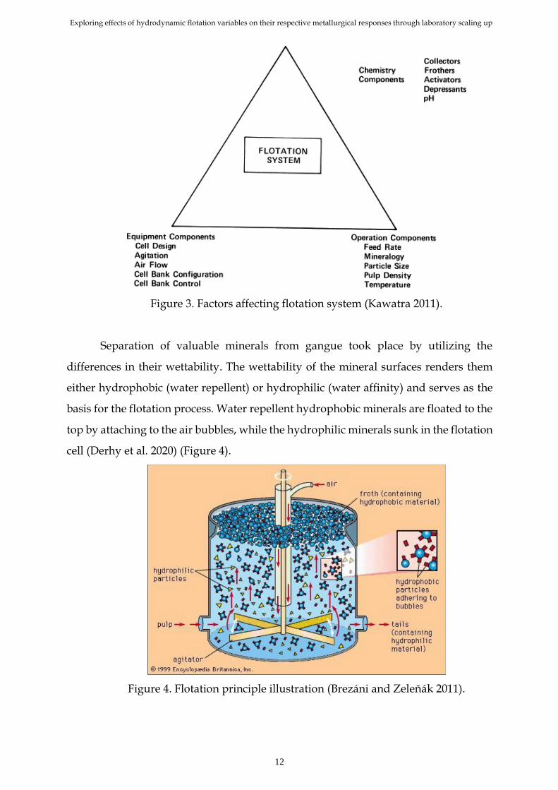
and pH) (Kawatra 2011) (Figure 3).
Exploring effects of hydrodynamic flotation variables on their respective metallurgical responses through laboratory scaling up
12
Figure 3. Factors affecting flotation system (Kawatra 2011).
Separation of valuable minerals from gangue took place by utilizing the
differences in their wettability. The wettability of the mineral surfaces renders them
either hydrophobic (water repellent) or hydrophilic (water affinity) and serves as the
basis for the flotation process. Water repellent hydrophobic minerals are floated to the
top by attaching to the air bubbles, while the hydrophilic minerals sunk in the flotation
cell (Derhy et al. 2020) (Figure 4).
Figure 4. Flotation principle illustration (Brezáni and Zeleňák 2011).

Exploring effects of hydrodynamic flotation variables on their respective metallurgical responses through laboratory scaling up
13
Few minerals such as coal and talc are naturally hydrophobic, while most of the
valuable minerals are hydrophilic. Hydrophobicity of the minerals can be increased by
increasing the contact angle which is created by the three different interfacial tensions.
In the three-phase flotation system, these interfacial tensions include solid-liquid (𝛾𝑠𝑙)
tension, solid-air (𝛾𝑠𝑎) tension and liquid-air (𝛾𝑙𝑎) tension (Figure 5).
Figure 5. The contact angle between the mineral surface and air bubble
(Nguyen 2013)
In the state of equilibrium, these three interfacial forces are defined through equation
(1) called the Young modulus equation (Rao 2004)
cos 휃 =
𝛾𝑠𝑎 − 𝛾𝑠𝑙
𝛾𝑙𝑎
(1)
Work of adhesion is defined as the force required to break the bubble-particle interface
and is given in the following mathematical equation
𝑊𝑠𝑎 = 𝛾𝑙𝑎 + 𝛾𝑠𝑙 − 𝛾𝑠𝑎
(2)
Contact angle (휃) thus can be defined by combining equation (1) and (2)
𝑊𝑠𝑎 = 𝛾𝑙𝑎(1 − cos 휃)
(3)

Exploring effects of hydrodynamic flotation variables on their respective metallurgical responses through laboratory scaling up
14
2.2 Flotation reagents
Different kinds of chemical reagents could be added to the flotation system called
surfactants for changing the contact angle and rendering specific surface properties on
the mineral surfaces and air bubbles. Accurate selection, optimum concentration, and
efficiency of the surfactant are key components for the success of any flotation process
(Bulatovic, 2014). Flotation reagents (surfactants) are broadly classified into three main
categories, collectors, frothers, and regulators.
2.2.1 Collectors
Collectors are organic compounds for selectively rendering hydrophobicity on
the surface of the desired minerals (Xing et al., 2017). For this purpose, they create a
water repellent layer through adsorption and provide necessary conditions for the
minerals to get themselves attached to the air bubble (Figure 6).
Figure 6. Collector adsorption on the surface of the mineral (Potapova, 2011).
Collectors are broadly categorized into two different groups, ionic and non-
ionic. Ionizing collectors have a complex asymmetric structure, consisting of polar and
non-polar parts. The polar part of the collector is the one that gets adsorbed on the

Exploring effects of hydrodynamic flotation variables on their respective metallurgical responses through laboratory scaling up
15
surface of the mineral, while the non-polar part is the hydrocarbon chain with water
repellent properties, thereby producing hydrophobicity (Figure 7).
Figure 7. Adsorption of the ionizing collector on the mineral water interface
extracted from (Nguyen 2013).
On the other hand, non-ionizing collectors lack the polar functional group and
only consist of hydrocarbon liquids. This type of collector is mostly used in those
minerals already having high contact angles and will only facilitate the fast attachment
to air bubbles such as coal, graphite, and talc. A schematic division of the collector is
shown in Figure 8.
Figure 8. Typical Classification of collector extracted from (Nguyen 2013)

Exploring effects of hydrodynamic flotation variables on their respective metallurgical responses through laboratory scaling up
16
Collectors adsorb themselves in the form of a monolayer on the surface of the
minerals in two ways, either through a chemically bound formation (chemisorption)
or via physical forces (physical adsorption) (Bulatovic, 2014).
Chemisorption involves a proper irreversible chemical reaction resulting in a
permanent change of the mineral surface. As chemisorption involves a chemical
reaction, it is highly selective as compared to physical adsorption, in which weak
attachment of the collector occurs on the surface of the mineral due to electrostatic or
Vander wall forces. Physical adsorption of the collector is reversible and less selective
(Bulatovic, 2014).
2.2.2 Frothers
Frothers play their role within the gas-liquid interface. The key function of the
frother is to stabilize the air bubbles with uniform size distribution. Similar to ionic
collectors, frothers are heteropolar molecules having both polar and non-polar parts.
The non-polar part of the frother adsorbed on the air bubble, whereas the polar part
gets dissolved in water (Figure 9). Important polar groups of frothers include carboxyl,
amine, hydroxyl, sulfur, and carbonyl groups. Some of the typical frothers include
polypropylene glycol ether, pine oil, methyl isobutyl carbinol (MIBC), xylenol (creslic
acid) (Table 1).
Figure 9. The action of frothers on the air bubble (Wills et al. 2006)

Exploring effects of hydrodynamic flotation variables on their respective metallurgical responses through laboratory scaling up
17
Table 1. Typical frothers used in froth flotation (Nguyen 2013)
2.2.3 Regulators
The chemical reagents are used in the froth flotation process to control the
solution chemistry can be categorized as regulators. Regulators include activators,
depressants, dispersants, and pH modifiers (Bulatovic, 2014). Activators are used
before the addition of the collector to alter the surface of the minerals, facilitating
enhanced collector adsorption. Activator thus acts as a bridge between the collector
and its adsorption on the mineral surface. Activators are mostly soluble salts with
common examples includes hydrosulfide, copper, and lead sulfate. Sodium sulfide is
an example of an activator used for the better adsorption of xanthate (collector) on the
surface of oxides minerals by forming a sulfide compound (Nguyen 2013). Depressants
play an opposite role as those of activators by blocking the adsorption of the collector
on certain mineral surfaces. In other words, they render hydrophilic nature to the
mineral surfaces. Polymer and Cyanide are common examples of depressants
(Pattanaik and Venugopal 2019). Often the flotation process occurs in alkaline pH as
commonly used collectors are stable at higher pH values. This condition also helps
avoid corrosion of flotation tanks and steel pipes that could happen in acidic
conditions, resulting in financial benefits. Alkaline conditions are controlled by adding
lime and soda ash and are categorized as pH modifiers (Zanin, Lambert, and du Plessis
2019).

Exploring effects of hydrodynamic flotation variables on their respective metallurgical responses through laboratory scaling up
18
2.3 Flotation circuits
Once the surface conditioning is done, the minerals are subjected to collide with
the air bubbles and get themselves attached; if there is no such contact, there will be
no flotation. This contact is attributed to three different probabilistic events, including
particle bubble Collison (Ec), particle bubble attachment (Ea), and particle bubble
stability (Es = 1- Ed, Ed being the probability of detachment) (Verrelli, Koh, and Nguyen
2011). Once the selective attachment of the particles to the air bubbles occurs, they are
transported to the top of the flotation cell, forming a froth layer due to the buoyancy
force. The particles and bubbles must not break apart while moving to the froth, where
they are removed by mechanical froth scrapers and sent to the next stage for further
purification. Particles can reach the froth zone due to any one of the following
phenomenon (Wills et al. 2006).
True flotation which is the selective attachment of the particles to the air
bubbles.
Entrainment resulting from the fine particles recovery in the water towards the
froth zone.
Entrapment, catching up of particles in between the air bubbles.
Out of these, true flotation is the one which is desirable as because of the other
two, gangue and undesired minerals can be recovered along with the valuable
minerals resulting in lowering of the grade. The flotation process is normally run in
several stages to increase the selective removal of the desired mineral particles through
true flotation (Figure 11). Rougher, Scavenger, and cleaner could be the three stages of
a flotation circuit. Running the flotation process in such circuits allows a much clean
recovery and desire grade by removing undesired particles that enter the concentrate
either due to entrainment or entrapment (Radmehr et al., 2018). Generally, a flotation
circuit consists of several such cells in series called a bank.

Exploring effects of hydrodynamic flotation variables on their respective metallurgical responses through laboratory scaling up
19
Figure 10. Basic flotation circuit, rougher, scavenger, and cleaner (Wills et al. 2006).
After passing the feed through size classification, it enters into the first stage of
the flotation circuit called rougher, where fast floating minerals are collected as
concentrate and tailings are sent to the scavenger stage to provide valuable minerals
with a second chance to float. The cleaner stage treats the rougher concentrate and
removes undesired minerals; hence, the targeted grade is achieved while keeping the
tailing’s grade as low as possible. These tailings are then recirculated back into the
rougher stage along with the rougher feed, while the cleaner's concentrate is
considered the final concentrate of the flotation circuit. On the other hand, scavenger
tailings are regarded as the final tailings. They can be subjected to regrinding along
with cleaner tailings to liberate valuable minerals (Radmehr et al., 2018).
2.4 Flotation equipment
Different flotation machines were developed in the past, broadly classifying them
into two categories, pneumatic and mechanical flotation machines (Wills et al. 2006).
These machines are differentiated based on bubble generating and froth cleaning
mechanism; however, the prominent distinguishing feature of column flotation from
mechanical is the spray of water from the top to the clean the concentrate (del Villar et
al. 2010). These machines are discussed below with important specifications.

Exploring effects of hydrodynamic flotation variables on their respective metallurgical responses through laboratory scaling up
20
2.4.1 Mechanical flotation machines
Mechanical flotation machines are the most widely used flotation machines in
the industry and are differentiated from pneumatic flotation machines based on the
froth cleaning mechanism and the use of impellers (Anderson 2017). Impellers are
considered as the heart of the mechanical flotation machines, responsible for important
functions such as creating necessary turbulence, breakdown of air bubbles into smaller
size, transfer of mechanical energy to the fluid, establishing a flow pattern, suspension
of solid particles, dispersion of gas bubbles and thus resulting in a bubble particle
collision (Shen et al. 2019; Wang et al. 2015a). Mechanical flotation machines have some
advantages over column flotation such as lesser water requirement per ton of feed,
better mixing of feed within the cell, lower blockage of the sparger, and elimination of
the technical problems that could arise due to height of the column as in column
flotation cells (Hacifazlioglu & Sutcu 2007; Al-Fariss et al. 2013; Jena et al. 2008). A
typical mechanical flotation machine is shown in Figure 11.
Figure 11. Typical mechanical flotation machine assembly (Strand et al. 2012)
Mechanical flotation machines are generally divided into three imaginary
hydrodynamic zones, namely, turbulent zone, quiescent zone, and froth zone (Wills et
al. 2006) shown in Figure 12. The turbulent zone lies below the other two-zone and is
termed turbulent because of the high turbulence in this region created by the impeller
or rotor. The turbulent zone is the most energy-intensive zone and plays an important

Exploring effects of hydrodynamic flotation variables on their respective metallurgical responses through laboratory scaling up
21
role in solid suspension, gas dispersion, and bubble particle collision (Meng et al.,
2016). The quiescent zone lies between the turbulent and froth zone, with relatively
less turbulence than the turbulent zone. The bubble particle aggregate develops in this
zone and rises to the froth zone along with entrapped gangue minerals (Wills et al.
2006). The Froth zone lies on the top where the froth stays momentarily before being
taken off by the scrapers. During this stay, cleaning the froth occurs due to the drop
back of loosely bounded hydrophobic and entrapped gangue minerals. Liquid
drainage, kinetic energy deceleration, and inertial impact of bubble particle aggregates
are the other reasons for the drop back of such mineral particles. Therefore, the overall
quality of the concentrate depends on the froth zone as it acts as an extra cleaning zone
before the froth is being removed (Yianatos et al., 2008).
Figure 12. Hydrodynamic zones in a mechanical flotation machine (Anon
2017)
2.4.2 Pneumatic flotation machines
Pneumatic flotation machines shown in Figure 14 are developed in the 1960s for
cleaning purposes, with the first real implementation took place in the mid-1980s. The
fundamental principle in these flotation cells is the counter-current flow of feed and
air. The air is injected from the bottom through an air sparging mechanism while the
feed is introduced near the mid-point of the flotation machine (Imhof et al. 2005) (Wills
et al., 2006). Particles thus travel down due to gravity while the air bubbles move in an
upward direction due to buoyancy force. This movement of particles and air bubbles

Exploring effects of hydrodynamic flotation variables on their respective metallurgical responses through laboratory scaling up
22
in opposite directions provides a way for the hydrophobic particles to collide and
attach themselves to the air bubbles. Apart from providing aeration conditions, the air
in pneumatic flotation machines is also responsible for the solid suspension and their
circulation. As a result of counter-current flow, column flotation cells provide
improved hydrodynamic conditions, lower power consumption, and a much cleaner
product compared to mechanical flotation machines (Bouchard et al., 2009). The ratio
of height to diameter in column flotation is important as it will define the interactive
distance between the particle and air bubbles. Most of the Industrial column flotation
cells have a height range from 6-14 m with a diameter of 0.5- 5 m (Wills et al. 2006)
(Lima, Peres, and Gonçalves 2018).
Column flotation possesses some advantages over mechanical flotation
machines, such as a high probability of collision between particles and bubbles,
simplicity of operation, fewer maintenance problems, higher separation efficiency,
lower capital and operating cost, low turbulence, lesser space requirement, and lower
residence time (Hacifazlioglu and Sutcu 2007; Lima et al. 2018; Wills, Napier-Munn,
and Wills 2006; Al-Fariss et al. 2013).
Unlike mechanical flotation machines, pneumatic flotation machines have two
hydrodynamic zones, namely, the collection zone and cleaning zone shown in Figure
13 (Wills et al. 2006) (Filippov, Royer, and Filippova 2017) (Tian et al. 2018). The
Collection zone of pneumatic flotation corresponds to 75-90 % of the total column
height, whereas the froth zone/collection zone corresponds to 10-25 % (Zheng,
Johnson, and Franzidis 2006). The Froth zone consists of more than 70 % of the air,
whereas the column zone consists of more or less 20 % of the air (del Villar et al., 2010).
Different phenomena occur in the collection zone of pneumatic flotation machines,
such as particle bubble attachment and detachment, entrainment and entrapping of
particles, etc. (Falutsu 1994). As a result, most of the hydrophobic and few of the
hydrophilic particles get attached to the air bubbles and are lifted to the froth zone of
the machines. Upon reaching the froth zone, a detachment phenomenon occurs in
which most of the hydrophilic and loosely bounded hydrophobic particles fall off the
froth zone. The spray of water in pneumatic flotation from the top causes the
entrapped hydrophilic particles to get detached and fall back (Wills et al. 2006).
Air is introduced in column flotation using internal spargers in the form of
porous or multi-nozzle spargers (Finch and Dobby 1991). Porous spargers are

Exploring effects of hydrodynamic flotation variables on their respective metallurgical responses through laboratory scaling up
23
commonly used on a laboratory scale, whereas multi-nozzle spargers are used on an
industrial scale using 15 – 20 spargers (Wills et al. 2006; Zheng et al. 2006; Finch and
Dobby 1991). Air is injected under high pressure of 30-100 psi through jet sparging of
air using orifices (Dobby 2002 2002). Such a sparger system requires no shut down of
operation if the spargers are required to be replaced (Dobby 2002).
Figure 13. Column flotation machines (Han et al. 2014)
2.4.3 Laboratory flotation machines
The beginning of any flotation experiment begins by running the pursued
flotation conditions on the laboratory scale. Due to lab-scale flotation cells, it is possible
to investigate flotation conditions relatively easier, faster, and cheaper than on the
industrial scale (Runge, K. 2010). Flotation tests can be repeated several times to cross-
validate the results under different conditions. A typical laboratory scale flotation test
begins with the size reduction of the material through a rod and ball mill. The
grounded material is passed through sieves to collect the feed's desired size, which is
then subjected to a flotation cell under desired conditions. The amount of feed varies
depending upon the volume of the flotation cell as well as the percentage solid. The
flotation conditions are run after conditioning time, with the froth being collected at a
chosen interval of time in empty trays. This collected froth is weighted both before and

Exploring effects of hydrodynamic flotation variables on their respective metallurgical responses through laboratory scaling up
24
after drying and placed in the oven to remove the water content. The weighted results
along with different chemical analyses, provide a way to find the grade, mass, and
water recovery. By plotting the cumulative distribution of recovery concerning time,
the analysis in terms of flotation rate constant provides a way to make certain
assumptions about the flotation process. Some commonly used laboratory flotation
machines include Hallimond tube, Modified Partridge- Smith cell, Outotec GTK lab
cell, etc.
2.5 Scale-up of flotation process
Over the past few decades, the flotation tank volume has increased to meet the
requirement of the mineral processing industry (the larger amount of ore to be
processed, the higher demand for metals/minerals). The mineral processing industry
is increasing both the number of flotation circuits and the dimension of the flotation
tanks. This shift towards large flotation tank dimensions holds several advantages,
such as it covers less space and involves lower capital, operational, maintenance,
energy, and reagent costs (Rinne and Peltola 2008). Earlier flotation tanks were less
than 1 m3. Currently, several flotation tanks with a volume as high as 300 m3 are
operational. Such an increase in flotation tank volume is termed scale-up, which
involves several technical, operational, and financial benefits. Figure 14 shows the
change in the flotation tank volume in this regard over the past few decades.

Exploring effects of hydrodynamic flotation variables on their respective metallurgical responses through laboratory scaling up
25
Figure 14. Increase in the flotation tank volume over the past century.
(Govender 2013b)
2.5.1 Economics of Up-scaling
One of the most important motivations for upscaling is the associated financial
benefits compared to smaller ones. The increase in the size of the flotation tank will
reduce their number, resulting in much lesser maintenance and operational costs.
(Rinne and Peltola 2008) have studied the major cost analysis associated with three
different volumes of flotation cells 100 m3, 200 m3, and 300 m3. Their study found that
the largest volume of the flotation cell involves the lowest overall cost when run under
optimized conditions. This study's major cost analysis includes investment cost,
reagent cost, maintenance cost, and energy consumption cost. The study was subjected
to financial evaluations over the whole life of flotation equipment (Figure 15).

Exploring effects of hydrodynamic flotation variables on their respective metallurgical responses through laboratory scaling up
26
Figure 15. Lifetime cost analysis of different flotation cells (Rinne and Peltola
2008)
Scale-up studies of froth flotation equipment are divided into the following two
categories;
1. Scale-up of flotation cells based on flotation kinetics.
2. Scale-up of flotation cells based on machine design.
2.5.2 Kinetic scale-up
The kinetic scale-up approach is commonly used for the scaling up of flotation
equipment. Researchers are agreed, kinetic models govern the flotation process if the
pulp is perfectly mixed and the solid particles are well suspended. The investigated
parameters are the recovery and grade of the minerals with respect to time. Kinetic
scale-up of flotation cells also forms the basis for the industrial scale-up of flotation
tanks (Mesa and Brito-Parada 2019). Different kinds of flotation kinetic models are
developed, and some of them are discussed below.
2.5.2.1 First-order approach
The first-order approach is established by considering the decrease in the
concentration of particles as a function of time (Vinnett and Waters 2020). The general
equation for this approach is shown in equation (4).
𝑑𝐶𝑝
𝑑𝑡= −𝑘1𝐶𝑝
(4)

Exploring effects of hydrodynamic flotation variables on their respective metallurgical responses through laboratory scaling up
27
In equation (4), 𝐶𝑝 shows the concentration of the particles, t represents the time
while 𝑘1 is the flotation rate constant. The negative sign indicates that the concentration
of particles is decreasing with respect to time. By solving the above differential
equation in terms of recovery (R), the following mathematical expression is obtained
𝑅 = 1 − 𝑒−𝑘1𝑡 (5)
The major concern for this model is the value of the flotation rate constant,
which keeps on changing during a flotation process. The value of the flotation rate
constant can be investigated through a laboratory batch test. Studies have shown that
no matter how optimum the conditions are. There always remains some amount of the
mineral that is impossible to float. The first-order approach in terms of maximum or
ultimate recovery (𝑅∞) is shown in equation (6) (Wills et al., 2006; Vinnett and Waters
2020).
𝑅 = 𝑅∞(1 − 𝑒−𝑘1𝑡)
(6)
Under perfect mixing conditions, recovery for the first-order approach can be
then calculated using equation (7).
𝑅 =𝑘1𝜏
1 + 𝑘1𝜏
(7)
2.5.2.2 Second-order approach
Second-order kinetics is another way of investigating the kinetics of the
flotation process. This model also considered the decreasing rate of particle
concentration. Equation (8) has shown the mathematical form of the second-order
approach.
𝑑𝐶𝑝
𝑑𝑡= −𝑘2𝐶𝑝
2
(8)
By integrating, the solution in terms of recovery is shown in equation (9).
𝑅 =𝑅∞
2 𝑘2𝑡
1 + 𝑅∞𝑘2𝑡
(9)
2.5.2.3 Klimpel approach

Exploring effects of hydrodynamic flotation variables on their respective metallurgical responses through laboratory scaling up
28
Klimpel (1980) presented the second-order flotation kinetic model by
introducing a rectangular distribution function. Equation (10) shows the Klimpel
model, kk being the modified form of first-order flotation rate constant.
𝑅 = 𝑅∞[1 −1
𝑘𝐾𝑡(1 − 𝑒−𝑘𝐾𝑡)]
(10)
2.5.2.4 Kelsall approach
Kelsall model explains the flotation kinetics by considering two different
flotation rate constants, one for the fast floating particles other for the slow floating
particles (X. Bu et al. 2017). Equation (11) shows the Kelsall model with kf is the
flotation rate constant for fast floating minerals, ks flotation rate constant for slow
floating minerals, and 𝜑 shows the percentage of the slow floating minerals.
𝑅 = (100 − 𝜑)(1 − 𝑒−𝑘𝑓𝑡) + 𝜑(1 − 𝑒−𝑘𝑠𝑡)
(11)
Table 2 shows the summary of different kinetics models with their mathematical
equations.
Table 2. A selection of flotation kinetic models.
Flotation Kinetic model
Mathematical equation
First-order approach 𝑅 =
𝑘1𝜏
1 + 𝑘1𝜏
Second-order approach 𝑅 =
𝑅∞2 𝑘2𝑡
1 + 𝑅∞𝑘2𝑡
Klimpel approach 𝑅 = 𝑅∞[1 −
1
𝑘𝐾𝑡(1 − 𝑒−𝑘𝐾𝑡)]
Kelsall approach 𝑅 = (100 − 𝜑)(1 − 𝑒−𝑘𝑓𝑡) + 𝜑(1 − 𝑒−𝑘𝑠𝑡)
Bu et al. (2017) has discussed different kinetic models for the flotation process.
In all of these flotation kinetic models, different parameters affecting the flotation
process are dealt with. Some of these models are derived based on experimental
studies, while others are formulated through mathematical/theoretical assumptions.
However, it is important to consider that the flotation rate constant derived during

Exploring effects of hydrodynamic flotation variables on their respective metallurgical responses through laboratory scaling up
29
laboratory investigations doesn’t hold the same relation as in the pilot and industrial
scale. This difference is due to the difference in hydrodynamic and other operational
conditions at these scales (Mesa and Brito-Parada 2019). Scaling up of flotation cells
through kinetic models from laboratory up to pilot and then to industrial scale is a
complex problem, which is why this phenomenon is not completely well solved and
is just a prediction of the relation between the two scales.
One approach is to define a scaling factor capable enough to correlate the
flotation conditions at different scales. For example, a scaling factor of 1.5 – 3 is
commonly used to estimate the industrial flotation rate constant through laboratory
flotation rate constant. The flotation rate constant for the industry is always considered
to be lower than the laboratory scale. This factor is obtained as a ratio of residence time
at an industrial scale to residence time at the laboratory. Finally, to achieve the
industrial flotation rate constant, the laboratory flotation rate is divided by this factor
(Mesa and Brito-Parada 2019).
Several mathematical models are developed to compare the kinetics of flotation
on different scales (laboratory and industry). Yianatos, Bergh, and Aguilera (2003) did
extensive work on up-scaling based on the kinetics model and developed separability
curves based on the ratio between mineral recovery and its yield, to get comparison
recovery. The point where the concentrate incremental recovery becomes equal to the
feed grade is considered as the comparison recovery. In one of the studies, they defined
scale-up factor based on the ratio of flotation rate constant in the lab to the flotation
rate constant on an industrial scale. The values of these two constants were obtained
by taking the average values for 10 months. Similarly, in another investigation, they
introduce a dimensionless scaling parameter that separates the effects of mixing and
kinetic changes on the scale-up factor, as shown in equation (12).
𝜏𝑃1𝑎𝑛𝑡
𝑡𝐿𝑎𝑏= 𝜙
𝑘𝐿𝑎𝑏
𝑘𝑃1𝑎𝑛𝑡 (12)
However, there exists a limitation in the above mathematical relation as the
defined equation ignores different hydrodynamic and equipment components such
tank size, solid segregation, and cell mixing. Therefore, the model is not a true
representation of the flotation process (Mesa and Brito-Parada 2019). (Yianatos et al.

Exploring effects of hydrodynamic flotation variables on their respective metallurgical responses through laboratory scaling up
30
2010) incorporated these effects in equation (13) to establish the scale-up factor (𝜉) by
considering the actual flotation rate constant𝑘𝑎𝑐.
𝜉 = 𝑘𝑎𝑐/𝑘𝐿𝑎𝑏 (13)
The actual or real flotation rate constant in the above equation is calculated
using the following relation
𝑘𝑎𝑐 =𝑘𝑎𝑝𝑝
휁휂𝜓
(14)
As shown, different parameters are incorporated, such as solid segregation(𝜓),
froth zone (휁 = 𝑘𝑎𝑝𝑝/𝑘𝑐) and cell mixing(휂). However, this equation also lacks
different sub-processes affecting the flotation rate constant, such as entrainment,
particle detachment during sampling, liquid drainage, and its transport in the froth
zone (Mesa and Brito-Parada, 2019). Gorain et al. (1998) discusses the kinetic scale up
by considering the influence of the ore characteristics, operating variables, and design
of the flotation cell through following mathematical relations
𝑘 = 𝑘𝑐𝑅𝑓 (15)
Where
𝑘𝑐 = 𝑃𝑆𝑏
(16)
𝑆𝑏 , defines the bubble surface area flux (𝑠−1), and is equal to 6𝐽𝑔/𝑑32. 𝐽𝑔 defines
the superficial gas velocity (𝑐𝑚
𝑠), 𝑑32 is the bubble Sauter mean diameter (mm), P is a
dimensionless parameter called floatability index categorizing ore characteristics. To
relate impeller design and other operating parameters to superficial gas velocity
𝑆𝑏 (Gorain et al. 1998) presented another mathematical model as shown in equation
(17).
𝑆𝑏 = 𝑎𝑁𝑠𝑏𝐽𝑔
𝑐𝐴𝑠𝑑𝑃80
𝑒 (17)
Ns represents the peripheral velocity of the impeller, As deals with the aspect
ratio between the impeller diameter and its height, P80 defines particle size, a, b, c, d,
and e are constants with values 1.23, 0.44, 0.75, −0.10 and−0.42, respectively. Values
of these constants are determined through experimental data analysis.
Exploring effects of hydrodynamic flotation variables on their respective metallurgical responses through laboratory scaling up
31
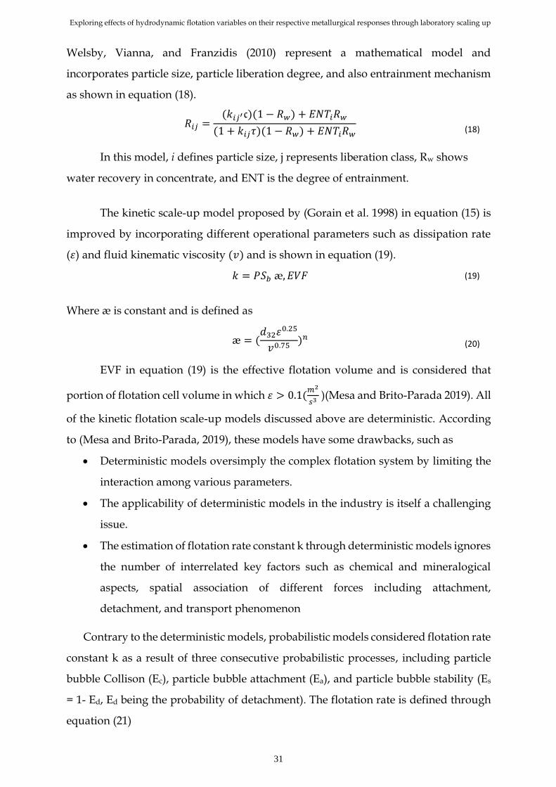
Welsby, Vianna, and Franzidis (2010) represent a mathematical model and
incorporates particle size, particle liberation degree, and also entrainment mechanism
as shown in equation (18).
𝑅𝑖𝑗 =
(𝑘𝑖𝑗′𝔠)(1 − 𝑅𝑤) + 𝐸𝑁𝑇𝑖𝑅𝑤
(1 + 𝑘𝑖𝑗𝜏)(1 − 𝑅𝑤) + 𝐸𝑁𝑇𝑖𝑅𝑤
(18)
In this model, i defines particle size, j represents liberation class, Rw shows
water recovery in concentrate, and ENT is the degree of entrainment.
The kinetic scale-up model proposed by (Gorain et al. 1998) in equation (15) is
improved by incorporating different operational parameters such as dissipation rate
(휀) and fluid kinematic viscosity (𝑣) and is shown in equation (19).
𝑘 = 𝑃𝑆𝑏 æ, 𝐸𝑉𝐹 (19)
Where æ is constant and is defined as
æ = (𝑑32휀0.25
𝑣0.75)𝑛
(20)
EVF in equation (19) is the effective flotation volume and is considered that
portion of flotation cell volume in which 휀 > 0.1(𝑚2
𝑠3 )(Mesa and Brito-Parada 2019). All
of the kinetic flotation scale-up models discussed above are deterministic. According
to (Mesa and Brito-Parada, 2019), these models have some drawbacks, such as
Deterministic models oversimply the complex flotation system by limiting the
interaction among various parameters.
The applicability of deterministic models in the industry is itself a challenging
issue.
The estimation of flotation rate constant k through deterministic models ignores
the number of interrelated key factors such as chemical and mineralogical
aspects, spatial association of different forces including attachment,
detachment, and transport phenomenon
Contrary to the deterministic models, probabilistic models considered flotation rate
constant k as a result of three consecutive probabilistic processes, including particle
bubble Collison (Ec), particle bubble attachment (Ea), and particle bubble stability (Es
= 1- Ed, Ed being the probability of detachment). The flotation rate is defined through
equation (21)

Exploring effects of hydrodynamic flotation variables on their respective metallurgical responses through laboratory scaling up
32
𝑘 = 𝑍𝑃 = 𝑍𝑃𝑐𝑃𝑎(1 − 𝑃𝑑)
(21)
Where Z is the bubble particle rate of collision.
Both the deterministic and probabilistic models for the kinetic scale-up of
flotation were considered only the pulp zone. Therefore, they were lacking any
influence of the different phenomena occurring in the froth zone. These issues are
tackled in machine design scale-up and are discussed in the next section.
2.5.3 Machine design scale-up
Machine design scale-up involves scale-up of the pulp zone while considering
the impact of the flotation equipment's design, size, and shape (Mesa and Brito-Parada,
2019). This is done by considering the simulated and dimensionless analysis on both
the laboratory and industrial scale with minimum compromise on flotation efficiency.
In this type of scale-up method, a suitable impeller type is defined first, which is
capable of meeting the required goals in terms of agitation conditions (Mesa and Brito-
Parada 2019). Other important factors such as number, speed, size, and energy
considerations of the impeller are analyzed in later scale-up stages. This scale-up
approach is the same as doing a scale-up and design of the continuous stirred tank
reactor CSTR in which the design of the large industrial tank is done with the same
mixing characteristics as on the laboratory scale (Mesa and Brito-Parada 2019).
While designing the scale-up of flotation equipment based on machine design,
impellers are the deciding factor. Different characteristics of the impeller and flotation
cell, such as geometric similarities, important ratios such as the ratio of impeller
diameter to the tank, the ratio of the width of impeller blade to its diameter, the ratio
of clearance of impeller from the bottom to the diameter of the tank/cell are important.
Similarly, dimensionless number, power, and energy consumption are among other
important considerations affecting the scale-up process (Mesa and Brito-Parada 2019).
(Arbiter, 2000) proposed the following mathematical equation (22) for impeller
diameter and rotational speed by keeping the power number and power per volume
(P/V) constant.
𝐷3 = 2.4022 + 0.0142𝑉
(22)
𝑁𝐷 = 6.66 + 0.0743𝑉 (23)

Exploring effects of hydrodynamic flotation variables on their respective metallurgical responses through laboratory scaling up
33
Bates, Fondy, and Corpstein (1963) studied the relation between power number
Np and Reynold number Re. They demonstrated Np becomes constant at higher values
of Re. This relation is shown in Figure 17 and is used to calculate the power
consumption for different types of impellers with different ratios of the width of
impeller blade W to the diameter of impeller D.
Figure 16. Relationship of Impeller's Reynold number and Power number
(Mesa and Brito-Parada 2019).
Different studies have kept the rotor tip speed (𝑉𝑡𝑖𝑝 = π𝑁𝐷) constant for the
scale-up process. Therefore, the nominal shear rate (�̇� =𝜋𝑁𝐷
𝛿) then also becomes
constant, as 𝛿 which is the shear gap width, is independent of the rotor-stator scale.
One of the fundamental problems with this scale-up criteria is that it only considers
the liquid phase and neglects the other two phases in the flotation cell, i.e., solid and
air, hence not a true representation of the flotation system (Mesa and Brito-Parada,
2019).
Just suspended is another criterion for the tank design and scale-up in which
minimum agitation speed is defined, for which all particles are in suspension. This
minimum agitation speed is found by considering the particles' maximum surface area
to be exposed in the fluid. The relation for the minimum agitation speed is shown in
equation (24).
Exploring effects of hydrodynamic flotation variables on their respective metallurgical responses through laboratory scaling up
34
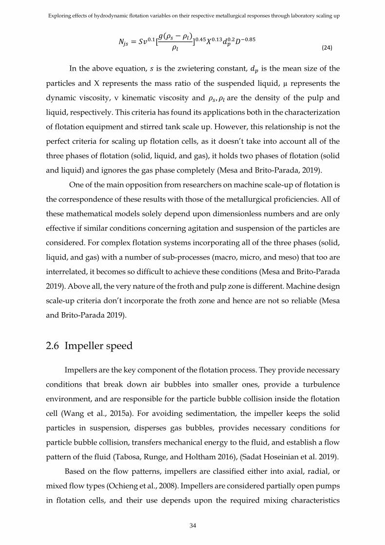
𝑁𝑗𝑠 = 𝑆𝑣0.1[𝑔(𝜌𝑠 − 𝜌𝑙)
𝜌𝑙]0.45𝑋0.13𝑑𝑝
0.2𝐷−0.85
(24)
In the above equation, 𝑠 is the zwietering constant, 𝑑𝑝 is the mean size of the
particles and X represents the mass ratio of the suspended liquid, µ represents the
dynamic viscosity, ν kinematic viscosity and 𝜌𝑠 , 𝜌𝑙 are the density of the pulp and
liquid, respectively. This criteria has found its applications both in the characterization
of flotation equipment and stirred tank scale up. However, this relationship is not the
perfect criteria for scaling up flotation cells, as it doesn’t take into account all of the
three phases of flotation (solid, liquid, and gas), it holds two phases of flotation (solid
and liquid) and ignores the gas phase completely (Mesa and Brito-Parada, 2019).
One of the main opposition from researchers on machine scale-up of flotation is
the correspondence of these results with those of the metallurgical proficiencies. All of
these mathematical models solely depend upon dimensionless numbers and are only
effective if similar conditions concerning agitation and suspension of the particles are
considered. For complex flotation systems incorporating all of the three phases (solid,
liquid, and gas) with a number of sub-processes (macro, micro, and meso) that too are
interrelated, it becomes so difficult to achieve these conditions (Mesa and Brito-Parada
2019). Above all, the very nature of the froth and pulp zone is different. Machine design
scale-up criteria don’t incorporate the froth zone and hence are not so reliable (Mesa
and Brito-Parada 2019).
2.6 Impeller speed
Impellers are the key component of the flotation process. They provide necessary
conditions that break down air bubbles into smaller ones, provide a turbulence
environment, and are responsible for the particle bubble collision inside the flotation
cell (Wang et al., 2015a). For avoiding sedimentation, the impeller keeps the solid
particles in suspension, disperses gas bubbles, provides necessary conditions for
particle bubble collision, transfers mechanical energy to the fluid, and establish a flow
pattern of the fluid (Tabosa, Runge, and Holtham 2016), (Sadat Hoseinian et al. 2019).
Based on the flow patterns, impellers are classified either into axial, radial, or
mixed flow types (Ochieng et al., 2008). Impellers are considered partially open pumps
in flotation cells, and their use depends upon the required mixing characteristics

Exploring effects of hydrodynamic flotation variables on their respective metallurgical responses through laboratory scaling up
35
(Souza Pinto et al., 2018). Axial impellers are used for solid suspension, whereas for
gas dispersion, radial impellers are widely used. For generating turbulence and shear
inside the flotation cell, Impellers are usually installed with a rotor-stator system. The
assembly of the impeller consists of a stator positioned around the impeller and acts
as an internal baffle. Appropriate design of baffles is important as it affects the stability
of froth (Anzoom et al. 2020). The stator converts the tangential flow of pulp into the
radial direction, resulting in gas dispersion and solid particles inside the tank. Several
blades arranged in a concentric way around the stator facilitates the flow of pulp inside
the tank. The flow of fluid (water) inside the tank occurs due to a pressure drop in the
center of the impeller. This results in continuous suction of liquid from the bottom into
the impeller. This flow then forms an ascending spiral swirl due to the agitation and
pumping action of the impeller (Anzoom et al., 2020). Figure 17 shows the rotor-stator
assembly inside the mechanical flotation machine.
Figure 17. Rotor, Stator assembly (Impeller) inside the flotation cell (Souza
Pinto et al. 2018).
The design of the impeller depends on the design of the flotation tank and its
performance within the tank (Wills, Napier-Munn, and Wills, 2006). Different factors
such as shape, size, stator blades, number of rotor and impeller angle effects the overall
performance of the impeller (Nelson and Lelinski 2000) (Shi et al. 2015), however, the
particle suspension, air drawn, and air dispersion were mainly influenced by the
design of rotor and stator (Wills, Napier-Munn, and Wills 2006).

Exploring effects of hydrodynamic flotation variables on their respective metallurgical responses through laboratory scaling up
36
Impeller speed is a key factor affecting the efficiency of the flotation process.
Increasing the impeller's speed also increases the flotation rate constant, collision
frequency, and the number of bubbles generated; however, collection efficiency is
decreased (Darabi et al., 2020). Bubble size, which is a critical parameter regarding the
efficiency of the flotation process, is affected by chemical (forth concentration) and
hydrodynamic factors (impeller speed, impeller design, and air flowrate) (Cilek, 2009)
(Nesset et al., 2006) (Laskowski, Cho, and Ding, 2008). The size of the bubble
distribution is characterized by either Sauter bubble diameter or through arithmetic
mean bubble diameter (Leiva et al., 2010). It is reported that the bubble size has an
inverse relation to the speed of the impeller and direct relation to that of the airflow
rate (Gorain, Franzidis, and Manlapig, 1995a). Mean bubble size has an inverse relation
with the impeller speed until a certain threshold value above which the impeller speed
will not cause any reduction in the size of bubble (Grau and Heiskanen 2005a; Grau
and Heiskanen 2005b; (Amini et al. 2013). Bubble size is also found to be location-
dependent regarding the impeller’s position, as large bubble sizes are found close to
the impeller shaft, and smaller bubble sizes are found at the discharge point (Gorain
et al. 1995a). Similarly, the effective solid suspension is an important factor for the
optimum flotation results, without which efficient bubble particle collision is
impossible (Amini, Bradshaw, and Xie 2016). Suspension of solids inside the flotation
cell depends upon the impeller speed, flow characteristics around the impeller, and
clearance between the bottom of the tank and the impeller (Wang et al. 2015a) (der
Westhuizen and Deglon, 2007; (Amini et al. 2016) (Schubert 1999). For the effective
solid suspension, critical impeller speed is defined, which is the minimum speed
keeping all solid particles in suspension, not allowing them to sediment/reside at the
bottom of the flotation tank (Lima, Deglon, and Leal Filho 2009). Critical speed is
considered to be the benchmark for the evaluation of solid suspension inside the
flotation machines and is found to be dependent upon various factors such as the size
of the particle, air flow rate, density, and concentration of solids inside the flotation
cell (van der Westhuizen and Deglon 2008). (Gorain, Franzidis, and Manlapig 1999)
mentioned that air bubble size is dependent upon the impeller’s air dispersion ability.
An increase in the impeller speed causes more fluid recirculation, hence increasing the
population of small size bubbles.

Exploring effects of hydrodynamic flotation variables on their respective metallurgical responses through laboratory scaling up
37
2.7 Airflow rate
In mechanical flotation machines, the air is introduced in two ways, either with
the help of external blowers or through the self-induction of air. In the case of the
blower, the air is injected at pressure, and the impeller is kept in the basement of the
cell. Whereas, in the case of self-induced, the impeller is kept in the midpoint of the
cell, drawing the air in between the space of the standpipe and the solid shaft (Gorain,
Franzidis, and Manlapig 2000).
Air flow rate is an important parameter for a successful flotation process. Some
more common ways of dealing with air flow rate are airflow number (Q/ND3), air flow
rate per cell volume (Q/V), or air flow velocity (Q/D2). In these equations, Q is the air
flow rate (L/min), N is the impeller speed (rpm), V is the volume of flotation cell (m3),
and D is impeller diameter (m) (Deglon, Egya-mensah, and Franzidis 2000). Another
way of describing air flow rate is superficial gas velocity, which is defined as a measure
of the aeration ability of a cell. Superficial gas velocity in mechanical flotation cells
varies from 0.6 to 1.5 cm s-1 depending upon the flotation cell type (rougher, scavenger,
or cleaner), impeller speeds, and airflow rate (Gorain et al. 2000). According to
(Schwarz and Alexander 2006), if the superficial velocity is higher than 3 cm/s, it will
result in poor flotation performance because of lesser froth stability and entrainment
issues. On the other hand, a value lower than 1 cm/s results in a lowering of flotation
kinetics.
Airflow rate affects the flotation rate constant by affecting different parameters
such as gas dispersion, bubble size distribution, and gas hold-up (Laplante, Toguri,
and Smith 1983) (Gorain, Franzidis, and Manlapig 1999). It has been noted that the
airflow rate has a positive effect on the recovery; however, the influence is more
predominant in the froth zone compared to any other region of the flotation cell. This
positive relation of airflow rate with the metallurgical response can be explained in
terms of froth residence time. Higher airflow rate values result in lesser residence time
in the froth zone, causing less bubble coalescence (Ata 2011). As bubble coalescence in
the froth zone is one reason for the detachment of the particles, this leads to higher
recoveries (Hadler et al., 2012). An increase in the airflow rate also increases the bubble
surface area, providing a higher chance for particle-bubble collision; hence, a higher
probability of bubble particle attachment (Hadler et al., 2012). However, the exceeding

Exploring effects of hydrodynamic flotation variables on their respective metallurgical responses through laboratory scaling up
38
air flow rate has a limitation, and after a certain point, their interaction would
unbalance the flotation hydrodynamics and reduce the process efficiency. Gorain,
Franzidis, and Manlapig (1995b) have shown that under constant impeller speed and
chemical conditions, an increase in the air flow rate results in an increase in the size of
the air bubble. This increase in bubble size is attributed to the reduction in the shear
forces which are responsible for the smaller bubble size. According to (Hadler et al.,
2012), lower values of airflow rate (superficial gas velocity) will result in lesser mobility
of the froth, resulting in the collapse of air bubbles and thus lower recovery. Similarly,
a higher value of air flow rate can assist entrainment and much quicker flow of forth.

Exploring effects of hydrodynamic flotation variables on their respective metallurgical responses through laboratory scaling up
39
Chapter 3
3 Materials and Methodology
In this study, the effect of impeller speed and airflow rate on flotation rate constant,
particle size, mass, and water recovery are analyzed on two different flotation cells (2L
and 7.5 L) of Outotec GTK LabCell®. Varying impeller speed and air flow rate under
the same chemical conditions were considered in these two cells. A schematic
representation of the flowsheet for this study is shown in Figure 18. Experimental work
was divided into two parts
Sample preparation
Flotation experiments.
Figure 18. Flowsheet for the sample preparation and flotation experiments.
For preparing a representative sample for each of the flotation experiments, 96
kg of pure olivine from Sibelco (Sweden) is subjected to grinding through rod mill
(primary stage) and ball mill (secondary stage). In total, 20 flotation tests were
designed based on the response surface methodology (RSM) for both the flotation cells
(2L and 7.5L). These flotation tests were then carried out under different combinations
of impeller speed and airflow rates. Flotation conditions are shown in table 4, which
were held constant. Effects of airflow rate were examined through the superficial gas
velocity and impeller speed on the impeller tip speed.

Exploring effects of hydrodynamic flotation variables on their respective metallurgical responses through laboratory scaling up
40
Table 3. Flotation conditions for flotation analysis.
Operating conditions for 2 L and 7.5 L flotation cell
Material Olivine
Weight of Olivine (2L cell) 750 grams
Weight of Olivine (7.5L cell) 2800 grams
Conditioning time 10 minutes
pH 10
Particle size < 106 µm
% solid 30
Collector Armeen C ( cationic collector)
Froth collecting time (cumulative) 1,3,5,7,10,15 (mint)
Collector dosage 1000 g / ton.
Basic solution (In case pH < 10) 5 % NaOH
Acidic solution (In case pH > 10) 5 % HCl
Investigated Impeller tip speeds (2L cell) 2.8, 3.06 and 3.3 (m/s)
Investigated superficial gas velocity (2L cell) 0.07, 0.14 and 0.21 (cm/s)
Investigated Impeller tip speeds (7.5 L cell) 2.8, 3.1 and 3.3 (m/s)
Investigated superficial gas velocity (7.5 cell) 0.07, 0.14 and 0.21 (cm/s)
Frothers, Activators, and Depressants -
3.1 Flotation equipment
Experimental works were performed in the Outotec GTK LabCell® shown in
Figure 19, which is a mechanical laboratory-scale batch flotation equipment.

Exploring effects of hydrodynamic flotation variables on their respective metallurgical responses through laboratory scaling up
41
Figure 19. Outotec GTK LabCell®.
This machine is comparable to other Outotec industrial scale flotation equipment
in terms of the design of the rotors and impellers with scale variations. Gas dispersion,
water addition, impeller speed, and air flow rate were controlled through an inbuilt
mechanism of the machine, with the only difference from industrial flotation tanks
being the periodic removal of froth using automatic scrapers. Figure 20 shows the
dimensions of the cells used in this experimental work. Their specifications are
tabulated in Table 5.
Figure 20. Different dimensions of Outotec GTK LabCells®.

Exploring effects of hydrodynamic flotation variables on their respective metallurgical responses through laboratory scaling up
42
Table 4. Manufacturer recommended machine parameters for the different scales
Cell Size
(Litre)
Rotor Diameter (mm) Rotor Speed
(rpm)
Air flow rate
(L / min)
2 45 1300 2
7.5 75 1200 4
3.2 Sample Preparation
3.2.1 Grinding and Sieving
Particle size distribution (PSD) analysis of the available feed (pure olivine)
indicates that most of the material was >106 µm (Figure 21), thus size reduction was
required. Therefore, the material was subjected to size reduction through grinding
using primary (rod mill) and secondary (ball mills). Parameters for both of the mills
are shown in Table 6.
Figure 21. Particle size distribution, available sample and flotation feed.
Exploring effects of hydrodynamic flotation variables on their respective metallurgical responses through laboratory scaling up
43
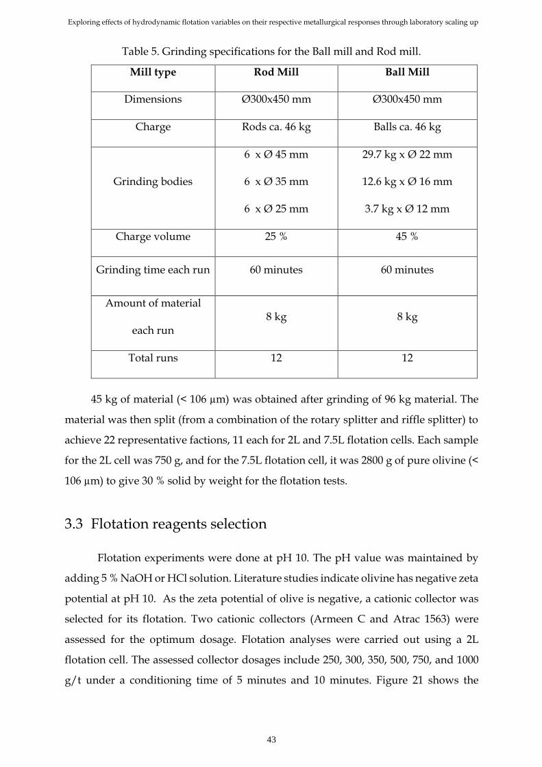
Table 5. Grinding specifications for the Ball mill and Rod mill.
Mill type Rod Mill Ball Mill
Dimensions Ø300x450 mm Ø300x450 mm
Charge Rods ca. 46 kg Balls ca. 46 kg
Grinding bodies
6 x Ø 45 mm
6 x Ø 35 mm
6 x Ø 25 mm
29.7 kg x Ø 22 mm
12.6 kg x Ø 16 mm
3.7 kg x Ø 12 mm
Charge volume 25 % 45 %
Grinding time each run 60 minutes 60 minutes
Amount of material
each run 8 kg 8 kg
Total runs 12 12
45 kg of material (< 106 µm) was obtained after grinding of 96 kg material. The
material was then split (from a combination of the rotary splitter and riffle splitter) to
achieve 22 representative factions, 11 each for 2L and 7.5L flotation cells. Each sample
for the 2L cell was 750 g, and for the 7.5L flotation cell, it was 2800 g of pure olivine (<
106 µm) to give 30 % solid by weight for the flotation tests.
3.3 Flotation reagents selection
Flotation experiments were done at pH 10. The pH value was maintained by
adding 5 % NaOH or HCl solution. Literature studies indicate olivine has negative zeta
potential at pH 10. As the zeta potential of olive is negative, a cationic collector was
selected for its flotation. Two cationic collectors (Armeen C and Atrac 1563) were
assessed for the optimum dosage. Flotation analyses were carried out using a 2L
flotation cell. The assessed collector dosages include 250, 300, 350, 500, 750, and 1000
g/t under a conditioning time of 5 minutes and 10 minutes. Figure 21 shows the
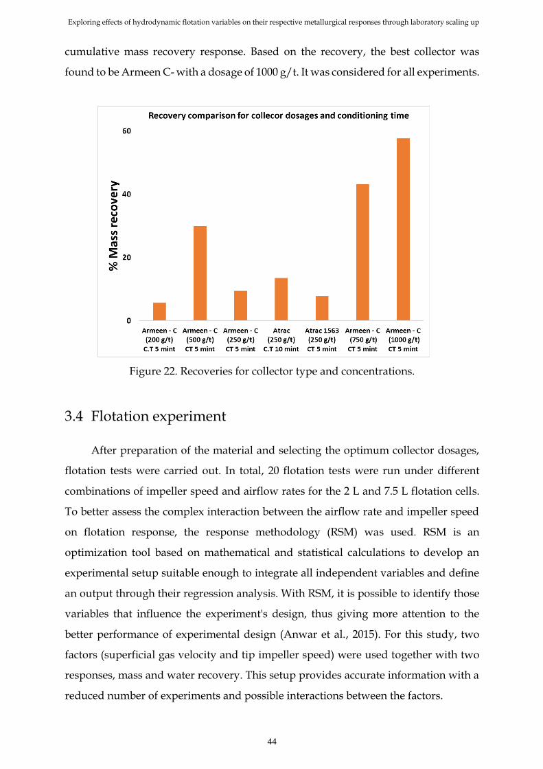
Exploring effects of hydrodynamic flotation variables on their respective metallurgical responses through laboratory scaling up
44
cumulative mass recovery response. Based on the recovery, the best collector was
found to be Armeen C- with a dosage of 1000 g/t. It was considered for all experiments.
Figure 22. Recoveries for collector type and concentrations.
3.4 Flotation experiment
After preparation of the material and selecting the optimum collector dosages,
flotation tests were carried out. In total, 20 flotation tests were run under different
combinations of impeller speed and airflow rates for the 2 L and 7.5 L flotation cells.
To better assess the complex interaction between the airflow rate and impeller speed
on flotation response, the response methodology (RSM) was used. RSM is an
optimization tool based on mathematical and statistical calculations to develop an
experimental setup suitable enough to integrate all independent variables and define
an output through their regression analysis. With RSM, it is possible to identify those
variables that influence the experiment's design, thus giving more attention to the
better performance of experimental design (Anwar et al., 2015). For this study, two
factors (superficial gas velocity and tip impeller speed) were used together with two
responses, mass and water recovery. This setup provides accurate information with a
reduced number of experiments and possible interactions between the factors.

Exploring effects of hydrodynamic flotation variables on their respective metallurgical responses through laboratory scaling up
45
Superficial gas velocity J𝑔 in cm/s is defined by equation (25), Q is the airflow
rate in cm3 / s, and A is the cross-sectional area of the cell (240 cm2 for 2L cell and 420
cm2 for 7.5 L flotation cell). Equation (26) is used to calculate Impeller tip speed (µ) in
meter/s; where D= impeller diameter in meter and N = Impeller rotational speed in
round per minute (rpm).
𝐽𝑔 =
𝑄
𝐴
(25)
µ = π D N
60
(26)
Based on the flotation cell analysis, under different impeller tip speeds and
superficial gas velocities, as shown in Appendix 1 and 2, three different impeller tip
speeds (2.8, 3.1, and 3.3 m/s) and three different superficial gas velocities (0.07, 0.14,
and 0.21 cm/s) were chosen for the experiments. The detailed set of experimental
conditions are shown in Table 7. Conditioning was carried out for 10 minutes, after
which the air was opened. In all experiments, there was no addition of feed once the
flotation conditions were run. As soon as froth formation has occurred, it was removed
through automatic scrappers, due to which the continuous lowering of both solid
concentrations and water content in the cell occurs. The Froth level was carefully
monitoring, and its height was maintained by adding water in the cell without
overflowing the froth. The froth is collected under cumulative time intervals of 1, 3, 5,
7, 10, and 15 minutes. The collected concentrates were then dried in an oven at 80 °C
for concentrate mass and water recovery analysis.

Exploring effects of hydrodynamic flotation variables on their respective metallurgical responses through laboratory scaling up
46
Table 6. Hydrodynamic conditions for flotation experiments in two different cells.
Number Hydrodynamic conditions
Std Run Superficial Gas Velocity (cm/s)
Impeller Tip Speed (m/s)
8 1 0.14 3.3
3 2 0.21 2.8
10 3 0.14 3.1
9 4 0.21 3.2
1 5 0.07 2.8
7 6 0.07 3.3
4 7 0.07 3.1
2 8 0.14 2.8
6 9 0.21 3.1
5 10 0.14 3.1

Exploring effects of hydrodynamic flotation variables on their respective metallurgical responses through laboratory scaling up
47
Chapter 4
4 Results
The main objective of this study was to understand the influence of hydrodynamic
parameters impeller speed (impeller tip speed) and airflow rate (superficial gas velocity)
on the laboratory scaling up of the Outotec GTK LabCell® flotation machine. The
representative metallurgical response, including mass and water recovery, particle size
distribution in the concentrate, and flotation kinetics, were studied with two different
mechanical flotation cells (2 liters and 7.5 liters).
4.1 Mass recovery analysis
Both 2 and 7.5 liters flotation cells were operated under 9 different combinations
of impeller tip speed and superficial gas velocity (Table 7). A time recovery curve was
plotted to analyze the behavior of cumulative recovery over the time interval of 1, 3, 5,
7, 10, and 15 minutes. These curves provide a much better and quicker analysis of
recovery. Figures 23 and 24 show the concentrate mass recovery for 2L and 7.5 L flotation
cells respectively. Metallurgical responses in terms of mass and water recovery are
shown in Table 8. The minimum value of concentrate mass recovery in the 2 L flotation
cell was 36.76 %, whereas, for the 7.5 L flotation cell, it was around 40.70 %. Similarly,
the maximum concentrate mass recovery was 61.47 and 85.84 % for 2 and 7.5 L flotation
cells, respectively. In other words, the results indicated that 7.5 L flotation cell showed
better performance compared to 2 L flotation cell under similar combinations. For the
2L flotation cell, more than 50 % of the overall recovery occurs during the first 7 minutes
of flotation, after which the maximum recovery R∞ is achieved, and the cumulative
recovery graphs reach their plateau. Similar behavior was found for the 7.5 L flotation
only in two conditions (superficial gas velocity 0.21 cm/s and impeller tip speed 3.1 and
3.3 m/s). A continuous increase in the cumulative mass recovery was observed for the
rest of the operating conditions, and the graph never reached its maximum recovery R∞.
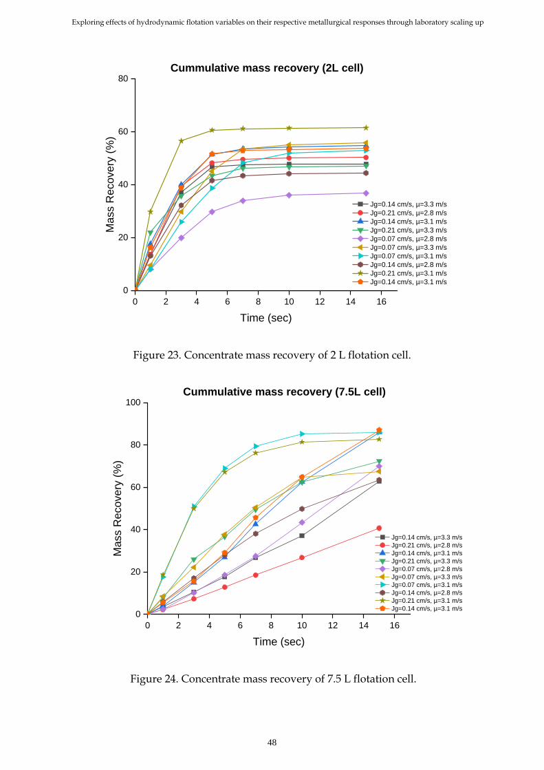
Exploring effects of hydrodynamic flotation variables on their respective metallurgical responses through laboratory scaling up
48
Figure 23. Concentrate mass recovery of 2 L flotation cell.
Figure 24. Concentrate mass recovery of 7.5 L flotation cell.
0 2 4 6 8 10 12 14 16
0
20
40
60
80
Jg=0.14 cm/s, µ=3.3 m/s
Jg=0.21 cm/s, µ=2.8 m/s
Jg=0.14 cm/s, µ=3.1 m/s
Jg=0.21 cm/s, µ=3.3 m/s
Jg=0.07 cm/s, µ=2.8 m/s
Jg=0.07 cm/s, µ=3.3 m/s
Jg=0.07 cm/s, µ=3.1 m/s
Jg=0.14 cm/s, µ=2.8 m/s
Jg=0.21 cm/s, µ=3.1 m/s
Jg=0.14 cm/s, µ=3.1 m/s
Mass R
ecovery
(%
)
Time (sec)
Cummulative mass recovery (2L cell)
0 2 4 6 8 10 12 14 16
0
20
40
60
80
100
Mass R
ecove
ry (
%)
Time (sec)
Jg=0.14 cm/s, µ=3.3 m/s
Jg=0.21 cm/s, µ=2.8 m/s
Jg=0.14 cm/s, µ=3.1 m/s
Jg=0.21 cm/s, µ=3.3 m/s
Jg=0.07 cm/s, µ=2.8 m/s
Jg=0.07 cm/s, µ=3.3 m/s
Jg=0.07 cm/s, µ=3.1 m/s
Jg=0.14 cm/s, µ=2.8 m/s
Jg=0.21 cm/s, µ=3.1 m/s
Jg=0.14 cm/s, µ=3.1 m/s
Cummulative mass recovery (7.5L cell)

Exploring effects of hydrodynamic flotation variables on their respective metallurgical responses through laboratory scaling up
49
Table 7. Summary table for concentrate mass and water recovery for both cells.
Operating conditions Flotation Cell 2 L Flotation Cell 7.5 L
Std Run
Superficial Gas
Velocity (cm/s)
Impeller Tip
Speed (m/s)
Cumulative mass
recovery %
Cumulative water
recovery %
Cumulative mass
recovery %
Cumulative water
recovery %
8 1 0.14 3.3 48.0 70.5 62.8 77.8
3 2 0.21 2.8 50.2 76.6 40.7 55.5
10 3 0.14 3.1 54.0 73.5 85.9 96.2
9 4 0.21 3.3 47.1 70.4 72.4 83.7
1 5 0.07 2.8 36.8 63.0 70.0 85.4
7 6 0.07 3.3 56.0 84.4 67.5 94.6
4 7 0.07 3.1 53.0 81.0 86.0 88.1
2 8 0.14 2.8 44.4 76.5 63.5 73.0
6 9 0.21 3.1 61.5 86.6 82.7 85.5
5 10 0.14 3.1 53.7 68.3 84.0 92.1
Box and whisker plots for non-cumulative mass recovery indicate consistent
results for all time intervals, as shown in Figure 25 and Figure 26 for the 2L and 7.5 L
flotation cells, respectively. The only exception occurred during 3 minutes of the
cumulative time interval for 7.5 L flotation cell where the tail of the box was more widely
spread, indicating a non-consistent behavior. This occurred due to much higher recovery
at the impeller tip speed of 3.1 and 3.3 m/s with the superficial gas velocity of 0.21 cm/s.
This higher recovery then affected the cumulative mass recovery during these two sets
of experiments and is indicated by the curve's flatness explained earlier.

Exploring effects of hydrodynamic flotation variables on their respective metallurgical responses through laboratory scaling up
50
Figure 25.Box and whisker plot for noncumulative mass recovery 2 L flotation cell
Figure 26. Box and whisker plot for noncumulative mass recovery 7.5 L flotation cell
4.2 Water recovery analysis
Figures 27 and 28 shows the cumulative water recovery analysis for all
combinations of impeller tip speed and superficial gas velocity for 2L and 7.5 L flotation
cells respectively. For the 2 L flotation cell, the highest value of water recovery was found

Exploring effects of hydrodynamic flotation variables on their respective metallurgical responses through laboratory scaling up
51
to be 86.63% at an impeller tip speed of 3.1 m /s and superficial gas velocity 0.21 cm/s,
whereas the lowest value was 62.94% at an impeller tip speed of 2.8 m/s and superficial
gas velocity of 0.07 cm/s. The maximum and minimum water recovery values for the
7.5 L flotation cell were 96.23 and 55.45 %, respectively. These values also occurred under
the same impeller tip speed and superficial gas velocity as for cumulative mass recovery.
For the 2L flotation cell, similar to cumulative mass recovery, the maximum water
recovery also reached R∞ after 7 min of flotation experiment; however, in 7.5 L of
flotation cell, water recovery never reached its R∞ as shown in Figure 28.
Figure 27.Cumulative water recovery 2L flotation cell.
0 2 4 6 8 10 12 14 16
0
20
40
60
80
100
Jg=0.14 cm/s, µ=3.3 m/s
Jg=0.21 cm/s, µ=2.8 m/s
Jg=0.14 cm/s, µ=3.1 m/s
Jg=0.21 cm/s, µ=3.3 m/s
Jg=0.07 cm/s, µ=2.8 m/s
Jg=0.07 cm/s, µ=3.3 m/s
Jg=0.07 cm/s, µ=3.1 m/s
Jg=0.14 cm/s, µ=2.8 m/s
Jg=0.21 cm/s, µ=3.1 m/s
Jg=0.14 cm/s, µ=3.1 m/s
Wate
r R
ecovery
(%
)
Time (sec)
Cummulative water recovery (2L cell)

Exploring effects of hydrodynamic flotation variables on their respective metallurgical responses through laboratory scaling up
52
Figure 28.Cumulative water recovery 7.5 L flotation cell.
The Box plots in Figures 29 and 30 show noncumulative water recovery at
different time intervals for the 2L and 7.5 L flotation cells, respectively. For the 2 L
flotation cell, the highest water recovery occurred during the first 5 min of the flotation
experiments, whereas for the 7.5 L flotation cell, water recovery was well distributed
throughout the flotation time. For the 2 L flotation cell, water recovery during the last 8
min of the flotation experiment was very low compared to the 7.5 L flotation cell. The
shape of box plots indicated a consistent behavior for the water recovery except for the
time interval of 3 minutes where the whisker of the box plots for both flotation cell
suggested the wide spreading of the water recovery compared to the rest of the time
intervals.
0 2 4 6 8 10 12 14 16
0
20
40
60
80
100
Jg=0.14 cm/s, µ=3.3 m/s
Jg=0.21 cm/s, µ=2.8 m/s
Jg=0.14 cm/s, µ=3.1 m/s
Jg=0.21 cm/s, µ=3.3 m/s
Jg=0.07 cm/s, µ=2.8 m/s
Jg=0.07 cm/s, µ=3.3 m/s
Jg=0.07 cm/s, µ=3.1 m/s
Jg=0.14 cm/s, µ=2.8 m/s
Jg=0.21 cm/s, µ=3.1 m/s
Jg=0.14 cm/s, µ=3.1 m/s
Wa
ter
Re
cove
ry (
%)
Time (sec)
Cummulative water recovery (7.5 L cell)

Exploring effects of hydrodynamic flotation variables on their respective metallurgical responses through laboratory scaling up
53
Figure 29. Box plot for noncumulative water recovery 2L cell.
Figure 30. Box plot for noncumulative water recovery 7.5L cell.
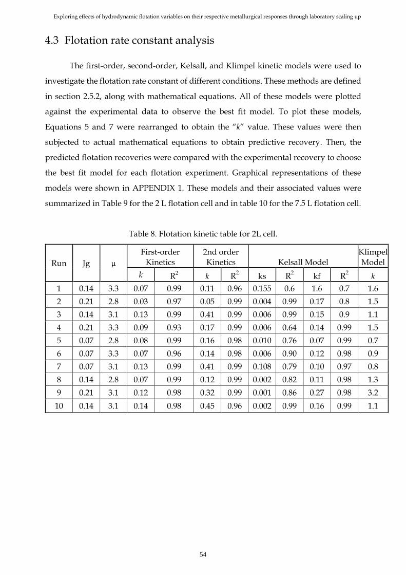
Exploring effects of hydrodynamic flotation variables on their respective metallurgical responses through laboratory scaling up
54
4.3 Flotation rate constant analysis
The first-order, second-order, Kelsall, and Klimpel kinetic models were used to
investigate the flotation rate constant of different conditions. These methods are defined
in section 2.5.2, along with mathematical equations. All of these models were plotted
against the experimental data to observe the best fit model. To plot these models,
Equations 5 and 7 were rearranged to obtain the “k” value. These values were then
subjected to actual mathematical equations to obtain predictive recovery. Then, the
predicted flotation recoveries were compared with the experimental recovery to choose
the best fit model for each flotation experiment. Graphical representations of these
models were shown in APPENDIX 1. These models and their associated values were
summarized in Table 9 for the 2 L flotation cell and in table 10 for the 7.5 L flotation cell.
Table 8. Flotation kinetic table for 2L cell.
Run Jg µ
First-order Kinetics
2nd order Kinetics Kelsall Model
Klimpel Model
k R2 k R2 ks R
2 kf R
2 k
1 0.14 3.3 0.07 0.99 0.11 0.96 0.155 0.6 1.6 0.7 1.6
2 0.21 2.8 0.03 0.97 0.05 0.99 0.004 0.99 0.17 0.8 1.5
3 0.14 3.1 0.13 0.99 0.41 0.99 0.006 0.99 0.15 0.9 1.1
4 0.21 3.3 0.09 0.93 0.17 0.99 0.006 0.64 0.14 0.99 1.5
5 0.07 2.8 0.08 0.99 0.16 0.98 0.010 0.76 0.07 0.99 0.7
6 0.07 3.3 0.07 0.96 0.14 0.98 0.006 0.90 0.12 0.98 0.9
7 0.07 3.1 0.13 0.99 0.41 0.99 0.108 0.79 0.10 0.97 0.8
8 0.14 2.8 0.07 0.99 0.12 0.99 0.002 0.82 0.11 0.98 1.3
9 0.21 3.1 0.12 0.98 0.32 0.99 0.001 0.86 0.27 0.98 3.2
10 0.14 3.1 0.14 0.98 0.45 0.96 0.002 0.99 0.16 0.99 1.1

Exploring effects of hydrodynamic flotation variables on their respective metallurgical responses through laboratory scaling up
55
Table 9. Flotation kinetic table for 7.5 L cell.
Run Jg µ
First-order Kinetics
2nd order Kinetics
Kelsall Model Klimpel Model
k R2 k R2 ks R
2 kf R2
k
1 0.07 3.1 0.09 0.99 0.17 0.98 0.86 0.97 0.04 0.98 0.79
2 0.07 2.8 0.07 0.99 0.14 0.97 0.04 0.98 0.04 0.99 0.21
3 0.14 3.1 0.13 0.99 0.41 0.96 0.18 0.99 0.06 0.99 0.21
4 0.14 3.3 0.12 0.99 0.32 0.98 0.07 0.98 0.09 0.99 0.45
5 0.07 3.3 0.03 0.98 0.05 0.99 0.20 0.98 0.04 0.99 0.25
6 0.21 2.8 0.08 0.99 0.16 0.97 0.05 0.78 0.04 0.98 0.51
7 0.21 3.1 0.07 0.99 0.11 0.99 0.04 0.73 0.23 0.99 0.87
8 0.14 2.8 0.12 0.99 0.12 0.99 0.06 0.9 0.08 0.99 0.35
9 0.21 3.3 0.13 0.99 0.41 0.99 0.03 0.8 0.22 0.98 1.16
10 0.14 3.1 0.45 0.98 0.45 0.95 0.18 0.92 0.06 0.99 0.35
Based on the best fit models, it was found that for the 2 L flotation cell, the 1st and
2nd order kinetic models could provide the best fits. Based on these results, the maximum
flotation rate constant was 0.11 min-1 for the superficial gas velocity of 0.21 cm/s and an
impeller tip speed of 3.1 m/s. In contrast, the minimum value was 0.03 min-1 for the
superficial velocity of 0.07 cm/s and an impeller tip speed of 2.8 m/s. For the 7.5 L
flotation cell, the 1st and 2nd order kinetic model provided the best fits. The maximum
value of the flotation rate constant of 0.45 min-1 was obtained in an experiment with the
superficial gas velocity of 0.14 cm/s and impeller tip speed of 3.1 m/s. The superficial
gas velocity of 0.07 cm/s and the impeller tip speed of 2.8 m/s caused the minimum
value of the flotation rate constant (0.03 min -1). Hence, the minimum value of the
flotation rate constant occurred at the same operating condition for both cells.
For the 2 L flotation cell, a direct relation was observed between the flotation rate
constant and the impeller tip speed at the superficial gas velocity of 0.0.07 cm/s. The
flotation rate constant increased from 0.03 to 0.05 min-1 by increasing the impeller tip
speed from 2.1 to 3.3 m/s. However, an inverse relation was observed in the case of the
superficial gas velocity of 0.21 cm /s by increasing the impeller tip speed from 2.8 to 3.3

Exploring effects of hydrodynamic flotation variables on their respective metallurgical responses through laboratory scaling up
56
m/s, causing a decrease in flotation rate constant from 0.05 to 0.04 min -1. For the
superficial gas velocity of 0.14 cm/ s, the flotation rate constant first increases and then
decreases by increasing the impeller tip speed from 2.8 to 3.3 m/s. Such a direct relation
was also observed at constant superficial gas velocities of 0.14 cm/s.
A similar direct relation was observed for the 7.5 L flotation cell between impeller
tip speed and flotation rate constant at the superficial gas velocity of 0.07 cm/s. k was
increased from 0.03 to 0.08 min-1 by increasing the impeller tip speed from 2.8 to 3.3 m
/s. Similar direct relation was also observed at the superficial gas velocity of 0.21 cm/s,
increasing the flotation rate constant from 0.07 to 0.13 min-1. However, in the case of the
superficial gas velocity of 0.14 cm/s, the flotation rate constant first increased from 0.12
to 0.13 min-1 by increasing the impeller tip speed from 2.8 to 3.1 m/s, and then decreased
to 0.09 min-1 when the impeller tip speed was further increased to 3.3 m/s.
4.4 Particle size distribution
Figure 31 shows the particle size distribution for the 2 L flotation cell at constant
superficial gas velocity and different impeller speeds. For all experimental conditions,
most of the particles in the concentrate were fine (-38 μm). In all combinations of impeller
tip speed and superficial gas velocity, the particle size greater than 38 μm constituted
less than 50 % of the total mass of concentrate.

Exploring effects of hydrodynamic flotation variables on their respective metallurgical responses through laboratory scaling up
57
Figure 31. Particle size distribution in different flotation setups for 2 L flotation cells
Figure 32 shows particle size distribution for the 7.5 L flotation cell. Contrary to
the 2 L flotation cell, particles in the 7.5 L flotation cell are relatively coarser (75-53 μm).
More than 40 % of the concentrate mass was in this size range in all of the experiments.
For the superficial gas velocity of 0.07 cm/s, an increase in the impeller tip speed
increased the mass fraction; however, for the other two values of superficial gas
velocities, an increase in the impeller tip speed resulted in the lowering of the mass
percentage in this range of size fraction.

Exploring effects of hydrodynamic flotation variables on their respective metallurgical responses through laboratory scaling up
58
Figure 32.Particle size distribution in different flotation setups for 7.5 L flotation cell.
4.5 Scale-up Assessment
4.5.1 Water recovery analysis
Figure 33 shows the scale-up assessment in terms of water recovery between 2 L
flotation cell and 7.5 L flotation cell by keeping the superficial gas velocity constant and
varying impeller tip speed. Based on the linear regression analysis, the coefficient of
determination (R2) showed the superficial velocity of 0.7 cm/s had a higher correlation
than the rest of the superficial gas velocities. Hence, for the scale-up assessment of
cumulative water recovery, the superficial gas velocity of 0.7 cm/s would perform well.

Exploring effects of hydrodynamic flotation variables on their respective metallurgical responses through laboratory scaling up
59
Figure 33. Scaling up assessments for water recovery based on the different impeller
tip speeds.
Similarly, for scale-up assessment of cumulative water recovery regarding
impeller tip speed, a similar comparison was considered where impeller tip speed was
kept constant and the superficial velocity is varied. As shown in Figure 34, an impeller
tip speed of 2.8 m/s involved higher R2 compared to an impeller tip speed of 3.1 and 3.3
m/s.

Exploring effects of hydrodynamic flotation variables on their respective metallurgical responses through laboratory scaling up
60
Figure 34. Scaling up assessment for water recovery based on different impeller tip
speeds.
4.5.2 Mass recovery analysis
Figure 35 shows the metallurgical response of cumulative mass recovery at
constant superficial gas velocity and different impeller tip speeds. Based on the linear
model fitting and R2, the superficial gas velocity of 0.21 cm/s indicated a much lower
R2, whereas Jg of 0.7 and 0.14 cm /sec provided a significantly higher correlation. Hence,
in scale-up for cumulative mass recovery, a superficial gas velocity of 0.7 cm/s and 0.14
cm/s will perform well.

Exploring effects of hydrodynamic flotation variables on their respective metallurgical responses through laboratory scaling up
61
Figure 35. Cumulative mass recovery scale-up assessment under constant superficial
gas velocity and different impeller tip speeds.
Figure 36 indicates a scale-up assessment for the metallurgical response of mass
recovery at constant impeller tip speed and varying superficial gas velocity, an impeller
tip speed of 2.8 m/s performs well compared to an impeller tip speed of 3.1 and 3.3 m/s.
Hence, for the scale-up assessment of mass recovery between 2 L and 7.5 L flotation cell,
an impeller tip speed of 2.8 m/s and superficial gas velocity of 0.7 cm/s could provide
a much better scale-up assessment.

Exploring effects of hydrodynamic flotation variables on their respective metallurgical responses through laboratory scaling up
62
Figure 36. Scaling up assessment for mass recovery based on same impeller tip speed
and different superficial gas velocities.
4.5.3 Scale-up Assessment flotation rate constant
The flotation rate constants derived in Tables 9 and 10 were used for the
multivariable scale-up assessments (considering variations of both parameters,
superficial gas velocity and impeller tip speed). Linear and nonlinear regression
indicated that none of the models fit accurately between the two cells based on various
flotation rate constant assessments, as shown in Figure 37. Scaling up between these two
flotation cells in terms of flotation rate constant is impossible while considering
variations of both hydrodynamic components simultaneously.

Exploring effects of hydrodynamic flotation variables on their respective metallurgical responses through laboratory scaling up
63
Figure 37. Model fitting for flotation rate constants between two cells.
However, considering the different impeller tip speeds and superficial gas
velocity of 0.21 cm/s, counterplotting for both cells indicates scaling up is possible as
shown in Figures 38 and 39.

Exploring effects of hydrodynamic flotation variables on their respective metallurgical responses through laboratory scaling up
64
Figure 38. Counter plots for flotation rate constant for 2L flotation cell.
Figure 39. Counter plots for flotation rate constant for 7.5L flotation cell.
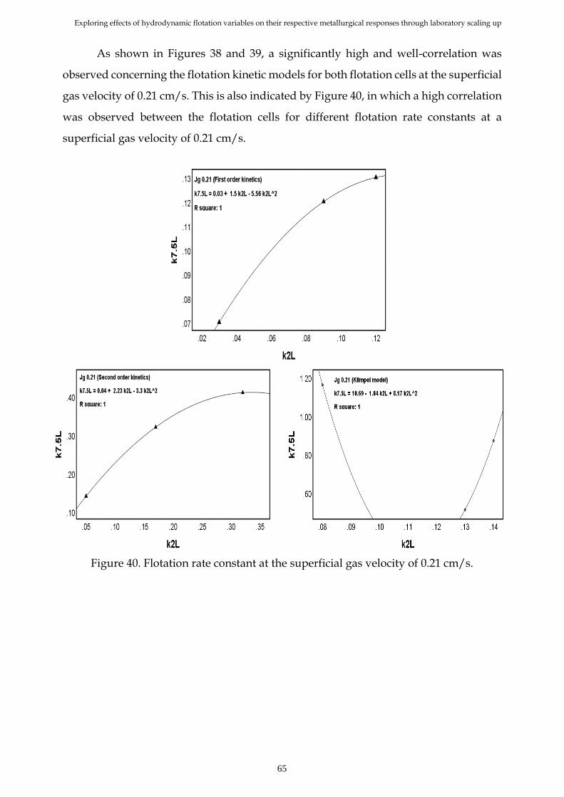
Exploring effects of hydrodynamic flotation variables on their respective metallurgical responses through laboratory scaling up
65
As shown in Figures 38 and 39, a significantly high and well-correlation was
observed concerning the flotation kinetic models for both flotation cells at the superficial
gas velocity of 0.21 cm/s. This is also indicated by Figure 40, in which a high correlation
was observed between the flotation cells for different flotation rate constants at a
superficial gas velocity of 0.21 cm/s.
Figure 40. Flotation rate constant at the superficial gas velocity of 0.21 cm/s.

Exploring effects of hydrodynamic flotation variables on their respective metallurgical responses through laboratory scaling up
66
Chapter 5
5 Discussion and Conclusions
5.1 Influence of Impeller tip speed
Varied impeller tip speed provided different metallurgical responses in the two
cells. The findings indicated that keeping the superficial gas velocity constant whilst
increasing the impeller tip speed from 2.8 to 3.1 m/s could result in an increase in the
mass and water recovery along with an increase in the flotation rate constant; however,
further increasing the impeller tip speed to 3.3 m/s resulted in a decrease in the
metallurgical responses. These results confirmed the research work of Schubert &
Bischofberger (1978). They have shown an increase in the recovery occurs at a constant
airflow rate and attributes it to the higher number of particle-bubble collisions due to
increasing impeller tip speed.
Various investigations have demonstrated that turbulence in a mechanical
flotation machine is a function of impeller speed. Tabosa (2012) showed that too much
turbulence has an adverse effect on froth stability, resulting in a lower recovery. As
turbulence depends upon the impeller tip speed, the decrease in the mass recovery
with increasing tip speed could be attributed to the detachment of the particles under
high turbulence. Nesset, Zhang & Finch (2012) showed an increase in impeller tip
speed at constant superficial gas velocity has no effects on bubble size; therefore,
increasing the impeller tip speed will enhance the detachment of the particles from the
bubbles at constant superficial gas velocity.
These results confirmed the flotation studies conducted by (Nesset, Zhang &
Finch 2012). In addition, researchers have demonstrated that the manner energy is
dissipated within the flotation cell is key to flotation efficiency. For example, Newell
& Grano (2006) reported that the flotation rate constant increases linearly with an
increase in energy dissipation. Results indicated by the 2 L flotation cell correlated well
with this hypothesis.
Exploring effects of hydrodynamic flotation variables on their respective metallurgical responses through laboratory scaling up
67
5.2 Influence of Airflow rate
The results indicated that increasing the superficial gas velocity increased the
metallurgical responses (concentrate mass and water recovery) for the 2 L cell. Hadler
et al. (2012) indicated that a lower value of superficial gas velocity results in lower
recoveries due to lesser froth mobility and collapsing air bubbles. In the case of
flotation rate constant, the particle size analysis suggested a higher percentage of fine
particles in concentrate for the 2 L flotation cell. (Wills et al. 2006) demonstrated that
the flotation rate depends upon the size of the particles and falls off when the particle
size is below an optimum range. This is due to a large number of particles getting
attached per unit weight of the air bubble, and the deteriorating effects of bubble-
particle attachment.
However, for the 7.5 L flotation cell, an increase in the superficial gas velocity
results in lowering the concentrate mass and water recoveries and the flotation rate
constant. Zhang Nesset, & Finch (2014) indicated that an increase in the superficial gas
velocity contributes towards increasing bubble size. Compared to smaller bubbles,
large size bubbles involve a lesser amount of particle attachment due to lesser surface
area. The 7.5 L flotation cell, as discussed earlier, involved less turbulence than the 2 L
flotation cell; hence, large size bubbles and lesser detachment probability. Heiskanen
(2000) reported that a low flotation rate constant at a higher value of superficial gas
velocity is due to a larger proportion of coarser particles in concentrate. The particle
size analysis for the 7.5 L flotation cell is in agreement with this statement.
5.3 Conclusion
Hydrodynamic components (impeller speed and airflow rate) are important
components for the successful mechanical flotation process. Impeller speed provides
necessary conditions that break down air bubbles into smaller ones, provide a
turbulent environment, affect flotation kinetics, and are responsible for the particle
bubble collision inside the flotation cell (Wang et al. 2015a). Similar to the impeller
speed, the airflow rate also affects the flotation rate constant (Laplante et al. 1983).
Some parameters such as gas dispersion, bubble size distribution, gas hold up, and
superficial gas velocity depends upon airflow rate behavior (Gorain et al. 1995). After

Exploring effects of hydrodynamic flotation variables on their respective metallurgical responses through laboratory scaling up
68
performing the experimental work and analyzing the results in terms of mass and
water recovery, flotation kinetics, and particle size distribution, metallurgical
responses showed scale up at laboratory scale is affected by both impeller speed and
airflow rate. Effects of impeller speed on the scale-up of lab-scale flotation machine
were analyzed through impeller tip speed of 2.8, 3.1, and 3.3 m/s, whereas the effect
of airflow rate was assessed through superficial gas velocities of 0.07, 0.14, and 0.21
cm/s.
It was found that for both of the flotation cells, the cumulative mass recovery
increased with an increase in the impeller tip speed from 2.8 to 3.1 m/s and then
decreased down if increased further to 3.3 m/s. Further, the percent cumulative mass
recovery in the 2 L flotation cell was lower compared to the 7.5 L flotation cell. This
decrease in the lower mass recovery could be attributed to higher turbulent conditions
inside the 2 L flotation cell compared to the 7.5 L flotation cell. This decrease in
recovery could be attributed to the detachment of the particles from air bubbles and
less collection efficiency at a higher value of impeller tip speed due to a much more
turbulent environment (Darabi et al. 2020). Newell and Grano (2006) reported that the
higher turbulence due to higher impeller speed, detachment of coarse particles could
occur along with the instability of the froth zone. This is well indicated by the much
lower presence of coarser particles in the concentrate mass of the 2 L flotation cell;
hence, verifying the high turbulence. For all of the operational hydrodynamic
conditions of the 7.5 L flotation cell, the cumulative mass recovery was significantly
higher compared to the 2 L flotation cell. Particle size distribution also suggested a
higher percentage of coarser particles in the concentrate mass for 7.5 L flotation cell,
confirming much better turbulent conditions.
Water recovery was also observed to be affected by impeller tip speed and
superficial gas velocity. For all of the operating conditions, water recovery was
significantly high in both flotation cells. Higher water recovery values indicated more
entrainment (Konopacka & Drzymala, 2010; Wang et al., 2015b). In both flotation cells,
the maximum and minimum values of the water recovery occurred under the same
hydrodynamic conditions. Water recovery was increased with an increase in the
impeller’s tip speed from 2.8 to 3.1 m/s but decreased if the impeller tip speed was
further increased. This showed that the overall water recovery for both the cells was
consistent under similar hydrodynamic conditions; however, for the 2 L flotation cell,
Exploring effects of hydrodynamic flotation variables on their respective metallurgical responses through laboratory scaling up
69
considerably higher water recovery was observed during the first 7 minutes. For 7.5 L
flotation cells, water recovery was well distributed over the whole flotation time. Flint
(2001) reported that higher water recovery indicated particle transportation through
entrainment. Assessing the particle size distribution confirmed the entrainment
process, as a higher percentage of fine particles were found in the concentrate mass of
the 2 L flotation cell. For the 2 L flotation cell, most of the cumulative mass recovery
also occurred during the first 7 minutes; hence, it could be deduced that entrainment
was mainly responsible for most of the cumulative mass recovery in the 2 L flotation
cell.
It has to take into account that these two cells did not symmetrically scale up
(they have a different ratio of X-Y-Z dimensions). However, the scale-up assessment
of laboratory Outotec mechanical flotation machines indicated that the flotation cells
having similar height/area ratio, mass, and water recovery scale-up assessment are
possible at an impeller tip speed of 2.8 m/s. Results also suggested that the flotation
kinetics between the two industrial scales was mainly influenced by the superficial gas
velocity compared to the impeller tip speed. In addition, the flotation rate constant was
more influenced by the superficial gas velocity as compared to the impeller tip speed.
Results released that kinetic assessment during scale-up of flotation cells was possible
at the superficial gas velocity of 0.21 cm/s.
This research work aimed to investigate the influence of hydrodynamic
parameters (impeller speed and airflow rate) on the scale-up of the Outotec GTK
LabCell®, flotation machine. Results obtained provide an initial investigation
regarding scaling up; however, it is recommended to incorporate some other
components responsible for the bubble-particle interaction, including gas holdup,
bubble velocity, and bubble size.

Exploring effects of hydrodynamic flotation variables on their respective metallurgical responses through laboratory scaling up
70
6 EIT Chapter
Today the raw material industry is facing two prominent challenges, 1) mineral
processing of lower grade ore bodies, 2) Higher demand for raw materials. To increase
the throughput, larger size froth flotation machines can play a key role in making it
possible to have a constant and sustainable production of raw materials. However, the
scaling-up involves a variety of macro and micro factors that influence the efficiency
of the process and will continue to be critical for the optimization of mineral
production both in terms of quality and quantity. The Outotec GTK LabCell®, a
mechanical flotation machine, has been used as a benchmark for many industrial pre-
feasibility studies worldwide for the past few decades. However, no published study
has evaluated the scaling-up indexes considering various floating cells, specifically
having similar height to area ratios (2 Liter and 7.5 Liter cells). The design of these lab
scale flotation machines is comparable to other Outotec industrial scale flotation
equipment considering rotor and impeller design, with the main difference being
scale-up. As stated in the thesis, economic study reveals that higher size flotation cells
require less capital and operational cost. This research focused on the influence of the
two most important hydrodynamic parameters, impeller speed and airflow rate, on
the scaling up. Results obtained will potentially contribute to improving the scaling-
up process resulting in the social, economic, and sustainable production of minerals
through froth flotation.
6.1 Recommendations for Future Work
Extend the range of investigated parameter values.
Evaluate hydrodynamic analysis on froth and turbulent zone separately.
Perform experimental work on other available flotation cells.
Incorporate other parameters such as different solid suspensions, gas hold-up,
energy dissipation, and bubble surface flux area.
Incorporate probabilistic models of attachment, detachment, and collision to
better understand the different particle size distributions' reasons in
concentrating at different hydrodynamic conditions.
Performing experimental work with different minerals to ascertain the
mineralogical effects affecting scaling up performances.

Exploring effects of hydrodynamic flotation variables on their respective metallurgical responses through laboratory scaling up
71
6.2 SWOT Analysis
Strength Weaknesses
Environmental friendly.
Cost-effective.
Repeatable
Requires less time
Availability of materials
Lower risk Involvement
Away from real-time conditions.
Novel Experimental work / few
experiences.
Less time considering experimental
work from material preparation
until performing result analysis.
Lack of reliable experimental work
on similar flotation machines
considering the similar objective.
Opportunities Threats
Repeating research work considering
other parameters affecting flotation.
Performing research work on other
flotation cells.
Extending the work to pilot-scale
studies.
Results are expected to differ when
the flotation feed is changed
The difference in the results at pilot
and industrial scale is expected.
Experimental work depends upon
operator expertise.
Cross-validation of the results is
not possible with previous research
work in this regard.

Exploring effects of hydrodynamic flotation variables on their respective metallurgical responses through laboratory scaling up
72
7 References Al-Fariss, T. F., K. A. El-Nagdy, F. A. Abd El-Aleem, and A. A. El-Midany. 2013. “Column
versus Mechanical Flotation for Calcareous Phosphate Fines Upgrading.” Particulate Science and Technology 31(5):488–93. doi: 10.1080/02726351.2013.776999.
Amini, E., D. J. Bradshaw, J. A. Finch, and M. Brennan. 2013. “Influence of Turbulence Kinetic Energy on Bubble Size in Different Scale Flotation Cells.” Minerals Engineering 45:146–50. doi: 10.1016/j.mineng.2013.01.015.
Amini, E., D. J. Bradshaw, and W. Xie. 2016. “Influence of Flotation Cell Hydrodynamics on the Flotation Kinetics and Scale up, Part 1: Hydrodynamic Parameter Measurements and Ore Property Determination.” Minerals Engineering 99:40–51. doi: 10.1016/j.mineng.2016.09.024.
Anderson, Corby. 2017. Flotation Equipment and Processes.
Ata, Seher. 2011. “Phenomena in the Froth Phase of Flotation — A Review.” International Journal of Mineral Processing 102:1–12. doi: 10.1016/j.minpro.2011.09.008
Rahman, Reza M., Seher Ata, and Graeme J. Jameson. "Study of froth behaviour in a controlled plant environment–Part 1: Effect of air flow rate and froth depth." Minerals Engineering 81 (2015): 152-160.. Anzoom, Sayed Janishar, Sunil Kumar Tripathy, Laxmikanta Sahu, S. Bhattacharya, and A.
K. Mukherjee. 2020. “Influence of Impeller Speed and Cell Volume on Coal Flotation Performance in a Self-Aerating Flotation Machine.” Advanced Powder Technology 31(9):4053–63. doi: 10.1016/j.apt.2020.08.008.
Bates, R. L., P. L. Fondy, and R. R. Corpstein. 1963. “Examination of Some Geometric Parameters of Impeller Power.” 5.
Bouchard, Jocelyn, André Desbiens, René del Villar, and Eduardo Nunez. 2009. “Column Flotation, Simulation and Control: An Overview.” Minerals Engineering 22(6):519–29. doi: 10.1016/j.mineng.2009.02.004.
Brezáni, Ivan, and Fridrich Zeleňák. 2011. “MATLAB Real-Time Data Acquisition for Laboratory Froth Flotation Automation.” Acta Montanistica Slovaca 16:176–83.
Bu, Xiangning, G. Xie, Yaoli Peng, Linhan Ge, and Chao Ni. 2017. “Kinetics of Flotation. Order of Process, Rate Constant Distribution and Ultimate Recovery.” Physicochemical Problems of Mineral Processing 53:342–65. doi: 10.5277/ppmp170128.
Bulatovic, S. M. (2014). Handbook of Flotation Reagents: Chemistry, Theory and Practice: Volume 3: Flotation of Industrial Minerals. Elsevier.
Cilek, Emin Cafer. 2009. “The Effect of Hydrodynamic Conditions on True Flotation and Entrainment in Flotation of a Complex Sulphide Ore.” Int. J. Miner. Process. 10.
Darabi, Hossna, S. M. Javad Koleini, David Deglon, Bahram Rezai, and Mahmoud Abdollahy. 2020. “Investigation of Bubble-Particle Attachment, Detachment and Collection Efficiencies in a Mechanical Flotation Cell.” Powder Technology 375:109–23. doi: 10.1016/j.powtec.2020.07.085.

Exploring effects of hydrodynamic flotation variables on their respective metallurgical responses through laboratory scaling up
73
Deglon, D. A., D. Egya-mensah, and J. P. Franzidis. 2000. “Review of Hydrodynamics and Gas Dispersion in Flotation Cells on South African Platinum Concentrators.” Minerals Engineering 13(3):235–44. doi: 10.1016/S0892-6875(00)00003-0.
Derhy, Manar, Yassine Taha, Rachid Hakkou, and Mostafa Benzaazoua. 2020. “Review of the Main Factors Affecting the Flotation of Phosphate Ores.” 20.
Dobby, Glenn. 2002. “Column Flotation.” 10.
Falutsu, M. 1994. “Column Flotation Froth Characteristics — Stability of the Bubble-Particle System.” International Journal of Mineral Processing 40(3–4):225–43. doi: 10.1016/0301-7516(94)90045-0.
Filippov, L. O., J. J. Royer, and I. V. Filippova. 2017. “Improvement of Ore Recovery Efficiency in a Flotation Column Cell Using Ultra-Sonic Enhanced Bubbles.” Journal of Physics: Conference Series 879:012023. doi: 10.1088/1742-6596/879/1/012023.
Finch, James A., and Glenn S. Dobby. 1991. “Column Flotation: A Selected Review. Part I.” International Journal of Mineral Processing 33(1–4):343–54. doi: 10.1016/0301-7516(91)90062-N.
Fuerstenau, Maurice C., Graeme J. Jameson, and R. H. Yoon. 2009. Froth Flotation a Century of Innovation. Littleton, Colo.: Society for Mining, Metallurgy, and Exploration.
Gorain, B., J. Franzidis, and E. Manlapig. 2000. “FLOTATION | Flotation Cell Design: Application of Fundamental Principles.”
Gorain, B. K., J. P. Franzidis, and E. V. Manlapig. 1995a. “Studies on Impeller Type, Impeller Speed and Air Flow Rate in an Industrial Scale Flotation Cell — Part 1: Effect on Bubble Size Distribution.” Minerals Engineering 8(6):615–35. doi: 10.1016/0892-6875(95)00025-L.
Gorain, B. K., J. P. Franzidis, and E. V. Manlapig. 1995b. “Studies on Impeller Type, Impeller Speed and Air Flow Rate in an Industrial Scale Flotation Cell — Part 1: Effect on Bubble Size Distribution.” Minerals Engineering 8(6):615–35. doi: 10.1016/0892-6875(95)00025-L.
Gorain, B. K., J. P. Franzidis, and E. V. Manlapig. 1999. “The Empirical Prediction of Bubble Surface Area Flux in Mechanical Flotation Cells from Cell Design and Operating Data.” Minerals Engineering 12(3):309–22. doi: 10.1016/S0892-6875(99)00008-4.
Gorain, B. K., J. P. Franzidis, and E. V. Manlapig. 1997. “Studies on Impeller Type, Impeller Speed and Air Flow Rate in an Industrial Scale Flotation Cell. Part 4: Effect of Bubble Surface Area Flux on Flotation Performance.” Minerals Engineering 10(4):367–79. doi: 10.1016/s0892-6875(97)00014-9.
Gorain, B. K., T. J. Napier-Munn, J. P. Franzidis, and E. V. Manlapig. 1998. “Studies on Impeller Type, Impeller Speed and Air Flow Rate in an Industrial Scale Flotation Cell. Part 5: Validation of k-Sb Relationship and Effect of Froth Depth.” Minerals Engineering 11(7):615–26. doi: 10.1016/S0892-6875(98)00046-6.
Govender, Devan. 2013a. “Large Flotation Cells in the Copper Processing Industry – Recent Experiences and Future Considerations (Part 1).” 11.

Exploring effects of hydrodynamic flotation variables on their respective metallurgical responses through laboratory scaling up
74
Govender, Devan. 2013b. “Large Flotation Cells in the Copper Processing Industry – Recent Experiences and Future Considerations (Part 1).” 11.
Grau, R. A., and K. Heiskanen. 2005a. “Bubble Size Distribution in Laboratory Scale Flotation Cells.” Minerals Engineering 18(12):1164–72. doi: 10.1016/j.mineng.2005.06.011.
Grau, R. A., and K. Heiskanen. 2005b. “Bubble Size Distribution in Laboratory Scale Flotation Cells.” Minerals Engineering 18(12):1164–72. doi: 10.1016/j.mineng.2005.06.011.
Hacifazlioglu, Hasan, and Hale Sutcu. 2007. “Optimization of Some Parameters in Column Flotation and a Comparison of Conventional Cell and Column Cell in Terms of Flotation Performance.” Journal of the Chinese Institute of Chemical Engineers 38(3–4):287–93. doi: 10.1016/j.jcice.2007.03.006.
Hadler, K., M. Greyling, N. Plint, and J. J. Cilliers. 2012. “The Effect of Froth Depth on Air Recovery and Flotation Performance.” Minerals Engineering 36–38:248–53. doi: 10.1016/j.mineng.2012.04.003.
Han, Oh-Hyung, Min-Kyu Kim, Byoung-Gon Kim, Nimal Subasinghe, and Chul-Hyun Park. 2014. “Fine Coal Beneficiation by Column Flotation.” Fuel Processing Technology 126:49–59. doi: 10.1016/j.fuproc.2014.04.014.
Heiskanen, Kari. 2000. “On the Relationship Between Flotation Rate and Bubble Surface Area Flux.” Minerals Engineering 13:141–49. doi: 10.1016/S0892-6875(99)00160-0.
Imhof, R., M. Battersby, F. Parra, and S. Sanchez-Pino. 2005. “The Successful Application of Pneumatic Flotation Technology for the Removal of Silica by Reverse Flotation at the Iron Ore Pellet Plant of Compañía Minera Huasco, Chile.” 8.
Jena, M. S., S. K. Biswal, S. P. Das, and P. S. R. Reddy. 2008. “Comparative Study of the Performance of Conventional and Column Flotation When Treating Coking Coal Fines.” Fuel Processing Technology 89(12):1409–15. doi: 10.1016/j.fuproc.2008.06.012.
Kawatra, Surendra. 2011. “Fundamental Principles of Froth Flotation.” SME Mining Engineering Handbook 1517–32.
Kesler, Stephen E. 2007. “Mineral Supply and Demand into the 21st Century.” 8.
Klimpel, R.R. Selection of chemical reagents for flotation. In Mineral Processing Plant Design; Mular, A.L.,Bhappu, R.B., Eds.; SME-AIME: New York, NY, USA, 1980; Volume 2, pp. 907–934.
Konopacka, Zaklina, and Jan Drzymala. 2010. “Types of Particles Recovery—Water Recovery Entrainment Plots Useful in Flotation Research.” Adsorption 16:313–20. doi: 10.1007/s10450-010-9246-x.
Laplante, A. R., J. M. Toguri, and H. W. Smith. 1983. “The Effect of Air Flow Rate on the Kinetics of Flotation. Part 2: The Transfer of Material from the Froth over the Cell Lip.” International Journal of Mineral Processing 11(3):221–34. doi: 10.1016/0301-7516(83)90027-3.
Laskowski, Janusz S., Yoon Seong Cho, and Kejian Ding. 2008. “Effect of Frothers on Bubble Size and Foam Stability in Potash Ore Flotation Systems.” The Canadian Journal of Chemical Engineering 81(1):63–69. doi: 10.1002/cjce.5450810107.

Exploring effects of hydrodynamic flotation variables on their respective metallurgical responses through laboratory scaling up
75
Leiva, J., L. Vinnett, F. Contreras, and J. Yianatos. 2010. “Estimation of the Actual Bubble Surface Area Flux in Flotation.” Minerals Engineering 23(11–13):888–94. doi: 10.1016/j.mineng.2010.01.013.
Lima, Neymayer Pereira, Antônio Eduardo Clark Peres, and Tatiane Aparecida Rocha Gonçalves. 2018. “Comparative Evaluation between Mechanical and Pneumatic Cells for Quartz Flotation in the Iron Ore Industry.” REM - International Engineering Journal 71(3):437–42. doi: 10.1590/0370-44672016710179.
Lima, O. A., D. A. Deglon, and L. S. Leal Filho. 2009. “A Comparison of the Critical Impeller Speed for Solids Suspension in a Bench-Scale and a Pilot-Scale Mechanical Flotation Cell.” Minerals Engineering 22(13):1147–53. doi: 10.1016/j.mineng.2009.05.002.
Matis, K. A., and P. Mavros. 1991. “Foam/Froth Flotation.” Separation & Purification Reviews 20(2):163–98.
Meng, Jun, Erico Tabosa, Weiguo Xie, Kym Runge, Dee Bradshaw, and Emmanuel Manlapig. 2016. “A Review of Turbulence Measurement Techniques for Flotation.” Minerals Engineering 95:79–95. doi: 10.1016/j.mineng.2016.06.007.
Mesa, Diego, and Pablo Brito-Parada. 2019. “Scale-up in Froth Flotation: A State-of-the-Art Review.” Separation and Purification Technology 210:950–62. doi: 10.1016/j.seppur.2018.08.076.
Mudd, Gavin M. 2007. “Global Trends in Gold Mining: Towards Quantifying Environmental and Resource Sustainability.” Resources Policy 32(1–2):42–56. doi: 10.1016/j.resourpol.2007.05.002.
Nelson, M. G., and D. Lelinski. 2000. “Hydrodynamic Design of Self-Aerating Flotation Machines.” Minerals Engineering 13(10–11):991–98. doi: 10.1016/S0892-6875(00)00085-6.
Nesset, J. E., Wei Zhang, and James Finch. 2012. A Benchmarking Tool for Assessing Flotation Cell Performance.
Nesset, Jan E., Jose R. Hernandez-Aguilar, Claudio Acuna, Cesar O. Gomez, and James A. Finch. 2006. “Some Gas Dispersion Characteristics of Mechanical Flotation Machines.” Minerals Engineering 19(6–8):807–15. doi: 10.1016/j.mineng.2005.09.045.
Newell, Ray, and Stephen Grano. 2006. “Hydrodynamics and Scale up in Rushton Turbine Flotation Cells: Part 2. Flotation Scale-up for Laboratory and Pilot Cells.” International Journal of Mineral Processing 81(2):65–78. doi: 10.1016/j.minpro.2006.07.002.
Nguyen, A. V. 2013. “Froth Flotation☆.” in Reference Module in Chemistry, Molecular Sciences and Chemical Engineering. Elsevier.
Ochieng, Aoyi, Maurice S. Onyango, Anil Kumar, Kirimi Kiriamiti, and Paul Musonge. 2008. “Mixing in a Tank Stirred by a Rushton Turbine at a Low Clearance.” Chemical Engineering and Processing: Process Intensification 47(5):842–51. doi: 10.1016/j.cep.2007.01.034.
Pattanaik, Abhyarthana, and Rayasam Venugopal. 2019. Role of Surfactants in Mineral Processing: An Overview. IntechOpen.

Exploring effects of hydrodynamic flotation variables on their respective metallurgical responses through laboratory scaling up
76
Radmehr, Vahid, Sied Ziaedin Shafaei, Mohammad Noaparast, and Hadi Abdollahi. 2018. “Optimizing Flotation Circuit Recovery by Effective Stage Arrangements: A Case Study.” Minerals 8(10):417. doi: 10.3390/min8100417.
Rao, S. Ramachandra. 2004. “Hydrophobicity and Contact Angle.” Pp. 351–84 in Surface Chemistry of Froth Flotation: Volume 1: Fundamentals, edited by S. R. Rao. Boston, MA: Springer US.
Rinne, Antti, and Aleksi Peltola. 2008. “On Lifetime Costs of Flotation Operations.” Minerals Engineering 21(12):846–50. doi: 10.1016/j.mineng.2008.04.018.
Runge, Kym. 2010. “Laboratory Flotation Testing – An Essential Tool for Ore Characterisation.” Flotation Plant Optimisation 19.
Sadat Hoseinian, Fatemeh, Bahram Rezai, Elaheh Kowsari, and Mehdi Safari. 2019. “Effect of Impeller Speed on the Ni(II) Ion Flotation.” Geosystem Engineering 22(3):161–68. doi: 10.1080/12269328.2018.1520651.
Schubert, Heinrich. 1999. “On the Turbulence-Controlled Microprocesses in Flotation Machines.” International Journal of Mineral Processing 56(1–4):257–76. doi: 10.1016/S0301-7516(98)00048-9.
Schubert, Heinrich, and Claus Bischofberger. 1978. “On the Hydrodynamics of Flotation Machines.” International Journal of Mineral Processing 5(2):131–42. doi: 10.1016/0301-7516(78)90010-8.
Schwarz, S., and D. Alexander. 2006. “Gas Dispersion Measurements in Industrial Flotation Cells.” Minerals Engineering 19(6–8):554–60. doi: 10.1016/j.mineng.2005.09.022.
Shen, Zhengchang, Ming Zhang, Xuesai Fan, Shuaixing Shi, and Dengfeng Han. 2019. “Hydrodynamic and Flotation Kinetic Analysis of a Large Scale Mechanical Agitated Flotation Cell with the Typical Impeller and the Arc Impeller.” Minerals 9(2):79. doi: 10.3390/min9020079.
Shi, Shuaixing, Ming Zhang, Xuesai Fan, and Dong Chen. 2015. “Experimental and Computational Analysis of the Impeller Angle in a Flotation Cell by PIV and CFD.” International Journal of Mineral Processing 142:2–9. doi: 10.1016/j.minpro.2015.04.029.
Souza Pinto, T. C., A. S. Braga, L. S. Leal Filho, and D. A. Deglon. 2018. “Analysis of Key Mixing Parameters in Industrial Wemco Mechanical Flotation Cells.” Minerals Engineering 123:167–72. doi: 10.1016/j.mineng.2018.03.046.
S .Razmjooei, M. Abdollahy, M. R. Khalesi, and M. Mohseni. 2017. “The Effect of Cross Section of Mechanical Flotation Cells on the Height of Turbulent and Quiescent Zones.” International Journal of Mining Science 3(4):89–92.
Strand, Anders, Dariusz Zasadowski, Magnus Norgren, Erik Hedenström, Stefan Willför, and A. Sundberg. 2012. “Selective Froth Flotation of Pitch Components from Spruce TMP Process Water.” Appita Journal 65:337–46.
Sulman, Henry Livingstone, Hugh Fitzalis Kirkpatrick-Picard, and John Ballot. 1906. “Ore Concentration.”
Tabosa, Erico. 2012. “The Effect of Cell Hydrodynamics on Flotation Kinetics.”
Exploring effects of hydrodynamic flotation variables on their respective metallurgical responses through laboratory scaling up
77
Tabosa, Erico, Kym Runge, and Peter Holtham. 2016. “The Effect of Cell Hydrodynamics on Flotation Performance.” International Journal of Mineral Processing 156:99–107. doi: 10.1016/j.minpro.2016.05.019.
Tian, Yahui, Xiaoli Luan, Fei Liu, and Stevan Dubljevic. 2018. “Model Predictive Control of Mineral Column Flotation Process.” Mathematics 6(6):100. doi: 10.3390/math6060100.
Verrelli, David I., Peter T. L. Koh, and Anh V. Nguyen. 2011. “Particle–Bubble Interaction and Attachment in Flotation.” Chemical Engineering Science 66(23):5910–21. doi: 10.1016/j.ces.2011.08.016.
del Villar, René, André Desbiens, Miguel Maldonado, and Jocelyn Bouchard. 2010. “Automatic Control of Flotation Columns.” Pp. 249–86 in Advanced Control and Supervision of Mineral Processing Plants, Advances in Industrial Control, edited by D. Sbárbaro and R. del Villar. London: Springer London.
Vinnett, Luis, and Kristian E. Waters. 2020. “Representation of Kinetics Models in Batch Flotation as Distributed First-Order Reactions.” Minerals 10(10):913. doi: 10.3390/min10100913.
Wang, L., Y. Peng, K. Runge, and D. Bradshaw. 2015a. “A Review of Entrainment: Mechanisms, Contributing Factors and Modelling in Flotation.” Minerals Engineering 70:77–91. doi: 10.1016/j.mineng.2014.09.003.
Wang, L., Y. Peng, K. Runge, and D. Bradshaw. 2015b. “A Review of Entrainment: Mechanisms, Contributing Factors and Modelling in Flotation.” Minerals Engineering 70:77–91. doi: 10.1016/j.mineng.2014.09.003.
Welsby, S. D. D., S. M. S. M. Vianna, and J. P. Franzidis. 2010. “Assigning Physical Significance to Floatability Components.” International Journal of Mineral Processing 97(1):59–67. doi: 10.1016/j.minpro.2010.08.002.
der Westhuizen, A. P. Van, and D. A. Deglon. 2007. “Evaluation of Solids Suspension in a Pilot-Scale Mechanical Flotation Cell: The Critical Impeller Speed.” Minerals Engineering 20(3):233–40. doi: 10.1016/j.mineng.2006.08.019.
van der Westhuizen, A. P., and D. A. Deglon. 2008. “Solids Suspension in a Pilot-Scale Mechanical Flotation Cell: A Critical Impeller Speed Correlation.” Minerals Engineering 21(8):621–29. doi: 10.1016/j.mineng.2007.12.010.
Vinnett, L., & Waters, K. E. (2020). Representation of Kinetics Models in Batch Flotation as Distributed First-Order Reactions. Minerals, 10(10), 913. https://doi.org/10.3390/min10100913
Wills, B. A., Tim Napier-Munn, and B. A. Wills. 2006. Wills’ Mineral Processing Technology: An Introduction to the Practical Aspects of Ore Treatment and Mineral Recovery. 7th ed. Amsterdam ; Boston, MA: Elsevier/BH.
Xing, Yaowen, Xiahui Gui, Fırat Karakas, and Yijun Cao. 2017. “Role of Collectors and Depressants in Mineral Flotation: A Theoretical Analysis Based on Extended DLVO Theory.” Minerals 7(11):223. doi: 10.3390/min7110223.
Yianatos, J. B., L. G. Bergh, and J. Aguilera. 2003. “Flotation Scale up: Use of Separability Curves.” Minerals Engineering 16(4):347–52. doi: 10.1016/S0892-6875(03)00024-4.

Exploring effects of hydrodynamic flotation variables on their respective metallurgical responses through laboratory scaling up
78
Yianatos, J. B., M. H. Moys, F. Contreras, and A. Villanueva. 2008. “Froth Recovery of Industrial Flotation Cells.” Minerals Engineering 21(12):817–25. doi: 10.1016/j.mineng.2007.12.012.
Yianatos, J., F. Contreras, P. Morales, F. Coddou, H. Elgueta, and J. Ortíz. 2010. “A Novel Scale-up Approach for Mechanical Flotation Cells.” Minerals Engineering 23(11):877–84. doi: 10.1016/j.mineng.2010.05.004.
Yianatos, Juan, Luis Bergh, F. Díaz, and Jorge Rodríguez. 2005. “Mixing Characteristics of Industrial Flotation Equipment.” Chemical Engineering Science 60:2273–82. doi: 10.1016/j.ces.2004.10.039.
Zanin, M., H. Lambert, and C. A. du Plessis. 2019. “Lime Use and Functionality in Sulphide Mineral Flotation: A Review.” Minerals Engineering 143:105922. doi: 10.1016/j.mineng.2019.105922.
Zhang, Wei, J. E. Nesset, and J. A. Finch. 2014. “Effect of Some Operational Variables on Bubble Size in a Pilot-Scale Mechanical Flotation Machine.” Journal of Central South University 21(3):1077–84. doi: 10.1007/s11771-014-2039-8.
Zheng, X., N. W. Johnson, and J. P. Franzidis. 2006. “Modelling of Entrainment in Industrial Flotation Cells: Water Recovery and Degree of Entrainment.” Minerals Engineering 19(11):1191–1203. doi: 10.1016/j.mineng.2005.11.005.

Exploring effects of hydrodynamic flotation variables on their respective metallurgical responses through laboratory scaling up
79
Appendix 1. 2 L Flotation Cell analysis for mass and water recovery
Variation of mass recovery with superficial gas velocity and tip speed
Variation of water recovery with superficial gas velocity and tip speed

Exploring effects of hydrodynamic flotation variables on their respective metallurgical responses through laboratory scaling up
80
Appendix 2. 7.5 L Flotation Cell analysis for mass and water recovery
Variation of mass recovery with superficial gas velocity and tip speed
Variation of water recovery with superficial gas velocity and tip speed

Exploring effects of hydrodynamic flotation variables on their respective metallurgical responses through laboratory scaling up
81
Appendix 3. Flotation model fitting 2L Cell Superficial gas velocity 0.14 cm/s and Impeller tip speed 3.3 m/s
0
20
40
60
80
100
0 5 10 15 20
CO
MM
ULA
TIV
E M
ASS
REC
OV
ERY
%
TIME (MIN)
FIRST ORDER KINETICS VS. EXPERIMENTAL DATA
EXPERIMENTAL DATA 1ST ORDER KINETICS
0
20
40
60
80
100
0 5 10 15 20
CO
MM
ULA
TIV
E M
ASS
REC
OV
ERY
%
TIME (MIN)
SECOND ORDER KINETICS VS. EXPERIMENTAL DATA
EXPERIMENTAL DATA 2ND ORDER KINETICS
0
20
40
60
80
100
0 5 10 15 20
CO
MM
ULA
TIV
E M
ASS
REC
OV
ERY
%
TIME (MIN)
KELSALL MODEL VS EXPERIMENTAL DATA
EXPERIMENTAL DATA KELSALL MODEL
0
20
40
60
80
100
0 5 10 15 20C
OM
MU
LATI
VE
MA
SS R
ECO
VER
Y %
TIME (MIN)
KLIMPEL MODEL VS. EXPERIMENTAL DATA
EXPERIMENTAL KLIMPEL MODEL

Exploring effects of hydrodynamic flotation variables on their respective metallurgical responses through laboratory scaling up
82
Superficial gas velocity 0.21 cm/s and Impeller tip speed 2.8 m/s
0
20
40
60
80
100
0 5 10 15 20
CO
MM
ULA
TIV
E M
ASS
REC
OV
ERY
%
TIME (MIN)
FIRST ORDER KINETICS VS. EXPERIMENTAL DATA
EXPERIMENTAL DATA 1ST ORDER KINETICS
0
20
40
60
80
100
0 5 10 15 20
CO
MM
ULA
TIV
E M
ASS
REC
OV
ERY
%
TIME (MIN)
SECOND ORDER KINETICS VS. EXPERIMENTAL DATA
EXPERIMENTAL DATA 2ND ORDER KINETICS
0
20
40
60
80
100
0 5 10 15 20
CO
MM
ULA
TIV
E M
ASS
REC
OV
ERY
%
TIME (MIN)
KLIMPEL MODEL VS. EXPERIMENTAL DATA
EXPERIMENTAL KLIMPEL MODEL
0
20
40
60
80
100
0 5 10 15 20
CO
MM
ULA
TIV
E M
ASS
REC
OV
ERY
%
TIME (MIN)
KELSALL MODEL VS EXPERIMENTAL DATA
EXPERIMENTAL DATA KELSALL MODEL

Exploring effects of hydrodynamic flotation variables on their respective metallurgical responses through laboratory scaling up
83
Superficial gas velocity 0.14 cm/s and Impeller tip speed 3.1 m/s
0
20
40
60
80
100
0 5 10 15 20
CO
MM
ULA
TIV
E M
ASS
REC
OV
ERY
%
TIME (MIN)
FIRST ORDER KINETICS VS. EXPERIMENTAL DATA
EXPERIMENTAL DATA 1ST ORDER KINETICS
0
20
40
60
80
100
0 5 10 15 20
CO
MM
ULA
TIV
E M
ASS
REC
OV
ERY
%
TIME (MIN)
SECOND ORDER KINETICS VS. EXPERIMENTAL DATA
EXPERIMENTAL DATA 2ND ORDER KINETICS
0
20
40
60
80
100
0 5 10 15 20
CO
MM
ULA
TIV
E M
ASS
REC
OV
ERY
%
TIME (MIN)
KLIMPEL MODEL VS. EXPERIMENTAL DATA
EXPERIMENTAL KLIMPEL MODEL
0
20
40
60
80
100
0 5 10 15 20
CO
MM
ULA
TIV
E M
ASS
REC
OV
ERY
%
TIME (MIN)
KELSALL MODEL VS EXPERIMENTAL DATA
EXPERIMENTAL DATA KELSALL MODEL

Exploring effects of hydrodynamic flotation variables on their respective metallurgical responses through laboratory scaling up
84
Superficial gas velocity 0.21 cm/s and Impeller tip speed 3.3 m/s
0
20
40
60
80
100
0 5 10 15 20
CO
MM
ULA
TIV
E M
ASS
REC
OV
ERY
%
TIME (MIN)
FIRST ORDER KINETICS VS. EXPERIMENTAL DATA
EXPERIMENTAL DATA 1ST ORDER KINETICS
0
20
40
60
80
100
0 5 10 15 20
CO
MM
ULA
TIV
E M
ASS
REC
OV
ERY
%
TIME (MIN)
SECOND ORDER KINETICS VS. EXPERIMENTAL DATA
EXPERIMENTAL DATA 2ND ORDER KINETICS
0
20
40
60
80
100
0 5 10 15 20
CO
MM
ULA
TIV
E M
ASS
REC
OV
ERY
%
TIME (MIN)
KELSALL MODEL VS EXPERIMENTAL DATA
EXPERIMENTAL DATA KELSALL MODEL
0
20
40
60
80
100
0 5 10 15 20
CO
MM
ULA
TIV
E M
ASS
REC
OV
ERY
%
TIME (MIN)
KLIMPEL MODEL VS. EXPERIMENTAL DATA
EXPERIMENTAL KLIMPEL MODEL

Exploring effects of hydrodynamic flotation variables on their respective metallurgical responses through laboratory scaling up
85
Superficial gas velocity 0.7 cm/s and Impeller tip speed 2.8 m/s
0
20
40
60
80
100
0 5 10 15 20
CO
MM
ULA
TIV
E M
ASS
REC
OV
ERY
%
TIME (MIN)
FIRST ORDER KINETICS VS. EXPERIMENTAL DATA
EXPERIMENTAL DATA 1ST ORDER KINETICS
0
20
40
60
80
100
0 5 10 15 20
CO
MM
ULA
TIV
E M
ASS
REC
OV
ERY
%
TIME (MIN)
SECOND ORDER KINETICS VS. EXPERIMENTAL DATA
EXPERIMENTAL DATA 2ND ORDER KINETICS
0
20
40
60
80
100
0 5 10 15 20
CO
MM
ULA
TIV
E M
ASS
REC
OV
ERY
%
TIME (MIN)
KELSALL MODEL VS EXPERIMENTAL DATA
EXPERIMENTAL DATA KELSALL MODEL
0
20
40
60
80
100
0 5 10 15 20
CO
MM
ULA
TIV
E M
ASS
REC
OV
ERY
%
TIME (MIN)
KLIMPEL MODEL VS. EXPERIMENTAL DATA
EXPERIMENTAL KLIMPEL MODEL

Exploring effects of hydrodynamic flotation variables on their respective metallurgical responses through laboratory scaling up
86
Superficial gas velocity 0.7 cm/s and Impeller tip speed 3.3 m/s
0
20
40
60
80
100
0 5 10 15 20
CO
MM
ULA
TIV
E M
ASS
REC
OV
ERY
%
TIME (MIN)
FIRST ORDER KINETICS VS. EXPERIMENTAL DATA
EXPERIMENTAL DATA 1ST ORDER KINETICS
0
20
40
60
80
100
0 5 10 15 20
CO
MM
ULA
TIV
E M
ASS
REC
OV
ERY
%
TIME (MIN)
SECOND ORDER KINETICS VS. EXPERIMENTAL DATA
EXPERIMENTAL DATA 2ND ORDER KINETICS
0
20
40
60
80
100
0 5 10 15 20
CO
MM
ULA
TIV
E M
ASS
REC
OV
ERY
%
TIME (MIN)
KELSALL MODEL VS EXPERIMENTAL DATA
EXPERIMENTAL DATA KELSALL MODEL
0
20
40
60
80
100
0 5 10 15 20
CO
MM
ULA
TIV
E M
ASS
REC
OV
ERY
%
TIME (MIN)
KLIMPEL MODEL VS. EXPERIMENTAL DATA
EXPERIMENTAL KLIMPEL MODEL

Exploring effects of hydrodynamic flotation variables on their respective metallurgical responses through laboratory scaling up
87
Superficial gas velocity 0.14 cm/s and Impeller tip speed 3.1 m/s
0
20
40
60
80
100
0 5 10 15 20
CO
MM
ULA
TIV
E M
ASS
REC
OV
ERY
%
TIME (MIN)
FIRST ORDER KINETICS VS. EXPERIMENTAL DATA
EXPERIMENTAL DATA 1ST ORDER KINETICS
0
20
40
60
80
100
0 5 10 15 20
CO
MM
ULA
TIV
E M
ASS
REC
OV
ERY
%
TIME (MIN)
SECOND ORDER KINETICS VS. EXPERIMENTAL DATA
EXPERIMENTAL DATA 2ND ORDER KINETICS
0
20
40
60
80
100
0 5 10 15 20
CO
MM
ULA
TIV
E M
ASS
REC
OV
ERY
%
TIME (MIN)
KELSALL MODEL VS EXPERIMENTAL DATA
EXPERIMENTAL DATA KELSALL MODEL
0
20
40
60
80
100
0 5 10 15 20
CO
MM
ULA
TIV
E M
ASS
REC
OV
ERY
%
TIME (MIN)
KLIMPEL MODEL VS. EXPERIMENTAL DATA
EXPERIMENTAL KLIMPEL MODEL
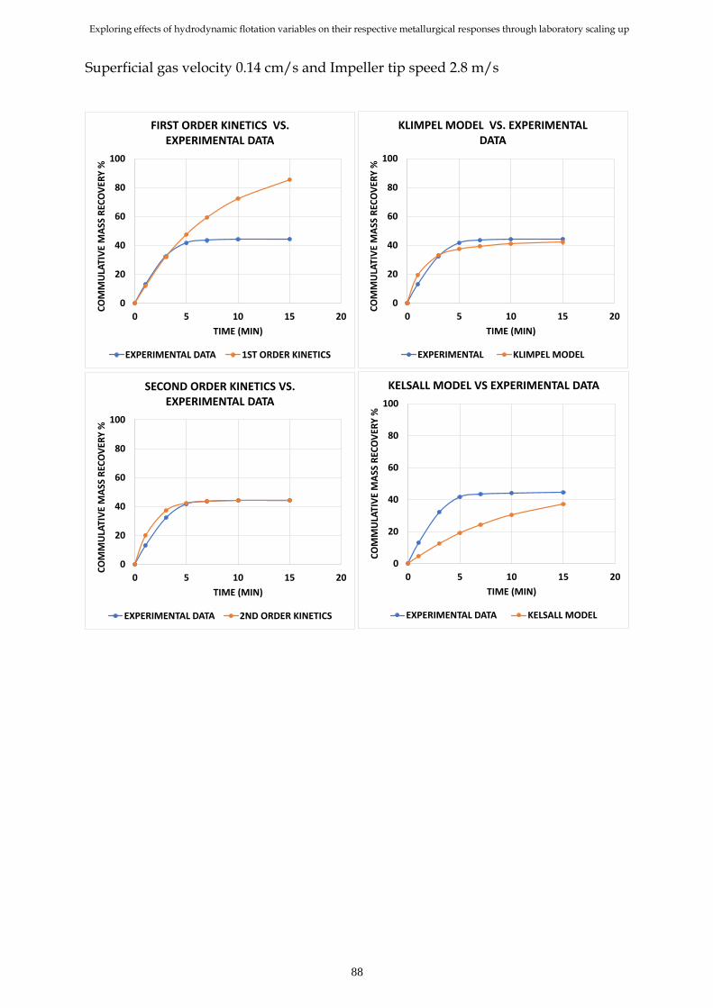
Exploring effects of hydrodynamic flotation variables on their respective metallurgical responses through laboratory scaling up
88
Superficial gas velocity 0.14 cm/s and Impeller tip speed 2.8 m/s
0
20
40
60
80
100
0 5 10 15 20
CO
MM
ULA
TIV
E M
ASS
REC
OV
ERY
%
TIME (MIN)
FIRST ORDER KINETICS VS. EXPERIMENTAL DATA
EXPERIMENTAL DATA 1ST ORDER KINETICS
0
20
40
60
80
100
0 5 10 15 20
CO
MM
ULA
TIV
E M
ASS
REC
OV
ERY
%
TIME (MIN)
SECOND ORDER KINETICS VS. EXPERIMENTAL DATA
EXPERIMENTAL DATA 2ND ORDER KINETICS
0
20
40
60
80
100
0 5 10 15 20
CO
MM
ULA
TIV
E M
ASS
REC
OV
ERY
%
TIME (MIN)
KELSALL MODEL VS EXPERIMENTAL DATA
EXPERIMENTAL DATA KELSALL MODEL
0
20
40
60
80
100
0 5 10 15 20
CO
MM
ULA
TIV
E M
ASS
REC
OV
ERY
%
TIME (MIN)
KLIMPEL MODEL VS. EXPERIMENTAL DATA
EXPERIMENTAL KLIMPEL MODEL
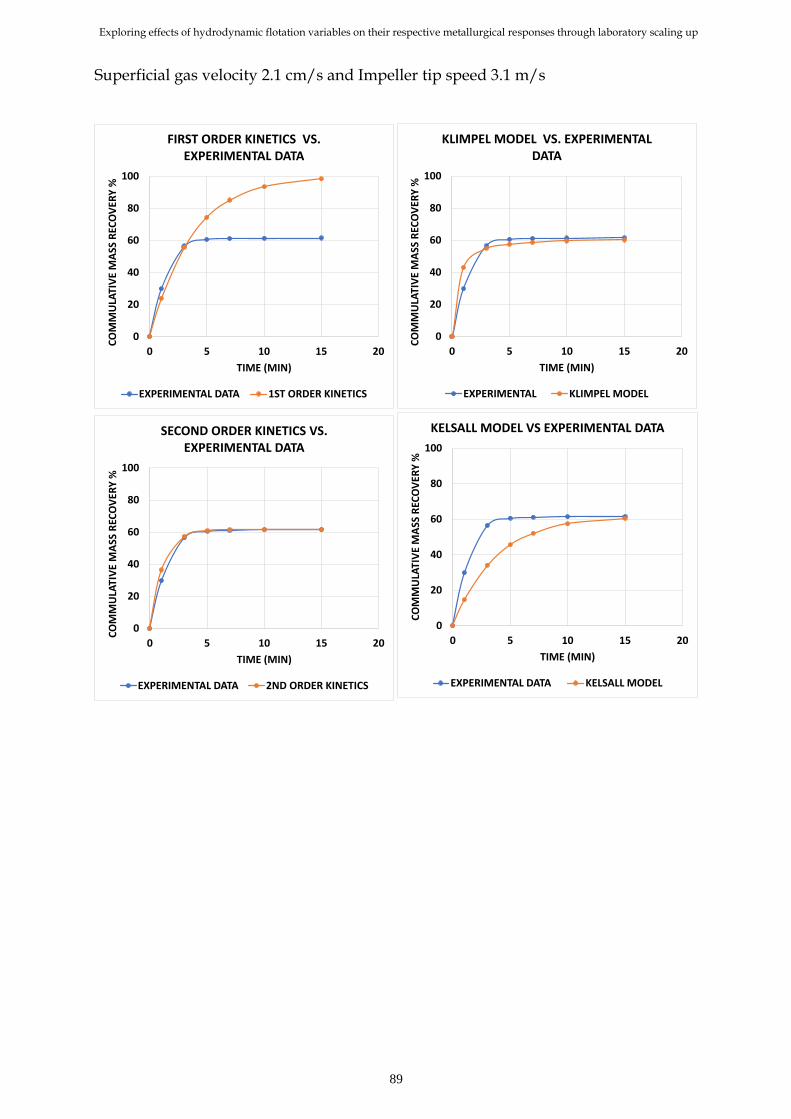
Exploring effects of hydrodynamic flotation variables on their respective metallurgical responses through laboratory scaling up
89
Superficial gas velocity 2.1 cm/s and Impeller tip speed 3.1 m/s
0
20
40
60
80
100
0 5 10 15 20
CO
MM
ULA
TIV
E M
ASS
REC
OV
ERY
%
TIME (MIN)
FIRST ORDER KINETICS VS. EXPERIMENTAL DATA
EXPERIMENTAL DATA 1ST ORDER KINETICS
0
20
40
60
80
100
0 5 10 15 20
CO
MM
ULA
TIV
E M
ASS
REC
OV
ERY
%
TIME (MIN)
SECOND ORDER KINETICS VS. EXPERIMENTAL DATA
EXPERIMENTAL DATA 2ND ORDER KINETICS
0
20
40
60
80
100
0 5 10 15 20
CO
MM
ULA
TIV
E M
ASS
REC
OV
ERY
%
TIME (MIN)
KELSALL MODEL VS EXPERIMENTAL DATA
EXPERIMENTAL DATA KELSALL MODEL
0
20
40
60
80
100
0 5 10 15 20
CO
MM
ULA
TIV
E M
ASS
REC
OV
ERY
%
TIME (MIN)
KLIMPEL MODEL VS. EXPERIMENTAL DATA
EXPERIMENTAL KLIMPEL MODEL

Exploring effects of hydrodynamic flotation variables on their respective metallurgical responses through laboratory scaling up
90
Superficial gas velocity 0.14 cm/s and Impeller tip speed 3.1 m/s
0
20
40
60
80
100
0 5 10 15 20
CO
MM
ULA
TIV
E M
ASS
REC
OV
ERY
%
TIME (MIN)
FIRST ORDER KINETICS VS. EXPERIMENTAL DATA
EXPERIMENTAL DATA 1ST ORDER KINETICS
0
20
40
60
80
100
0 5 10 15 20
CO
MM
ULA
TIV
E M
ASS
REC
OV
ERY
%
TIME (MIN)
SECOND ORDER KINETICS VS. EXPERIMENTAL DATA
EXPERIMENTAL DATA 2ND ORDER KINETICS
0
20
40
60
80
100
0 5 10 15 20
CO
MM
ULA
TIV
E M
ASS
REC
OV
ERY
%
TIME (MIN)
KELSALL MODEL VS EXPERIMENTAL DATA
EXPERIMENTAL DATA KELSALL MODEL
0
20
40
60
80
100
0 5 10 15 20
CO
MM
ULA
TIV
E M
ASS
REC
OV
ERY
%
TIME (MIN)
KLIMPEL MODEL VS. EXPERIMENTAL DATA
EXPERIMENTAL KLIMPEL MODEL

Exploring effects of hydrodynamic flotation variables on their respective metallurgical responses through laboratory scaling up
91
ANNEX 4 FLOTATION MODEL FITTING 7.5 L CELL. Superficial gas velocity 0.14 cm/s and Impeller tip speed 3.3 m/s
0
20
40
60
80
100
0 5 10 15 20
CO
MM
ULA
TIV
E M
ASS
REC
OV
ERY
%
TIME (MIN)
FIRST ORDER KINETICS VS. EXPERIMENTAL DATA
EXPERIMENTAL DATA 1ST ORDER KINETICS
0
20
40
60
80
100
0 5 10 15 20
CO
MM
ULA
TIV
E M
ASS
REC
OV
ERY
%
TIME (MIN)
SECOND ORDER KINETICS VS. EXPERIMENTAL DATA
EXPERIMENTAL DATA 2ND ORDER KINETICS
0
20
40
60
80
100
0 5 10 15 20
CO
MM
ULA
TIV
E M
ASS
REC
OV
ERY
%
TIME (MIN)
KELSALL MODEL VS EXPERIMENTAL DATA
EXPERIMENTAL DATA KELSALL MODEL
0
20
40
60
80
100
0 5 10 15 20C
OM
MU
LATI
VE
MA
SS R
ECO
VER
Y %
TIME (MIN)
KLIMPEL MODEL VS. EXPERIMENTAL DATA
EXPERIMENTAL KLIMPEL MODEL

Exploring effects of hydrodynamic flotation variables on their respective metallurgical responses through laboratory scaling up
92
Superficial gas velocity 0.21 cm/s and Impeller tip speed 2.8 m/s
0
20
40
60
80
100
0 5 10 15 20
CO
MM
ULA
TIV
E M
ASS
REC
OV
ERY
%
TIME (MIN)
FIRST ORDER KINETICS VS. EXPERIMENTAL DATA
EXPERIMENTAL DATA 1ST ORDER KINETICS
0
20
40
60
80
100
0 5 10 15 20
CO
MM
ULA
TIV
E M
ASS
REC
OV
ERY
%
TIME (MIN)
SECOND ORDER KINETICS VS. EXPERIMENTAL DATA
EXPERIMENTAL DATA 2ND ORDER KINETICS
0
20
40
60
80
100
0 5 10 15 20
CO
MM
ULA
TIV
E M
ASS
REC
OV
ERY
%
TIME (MIN)
KELSALL MODEL VS EXPERIMENTAL DATA
EXPERIMENTAL DATA KELSALL MODEL
0
20
40
60
80
100
0 5 10 15 20
CO
MM
ULA
TIV
E M
ASS
REC
OV
ERY
%
TIME (MIN)
KLIMPEL MODEL VS. EXPERIMENTAL DATA
EXPERIMENTAL KLIMPEL MODEL

Exploring effects of hydrodynamic flotation variables on their respective metallurgical responses through laboratory scaling up
93
Superficial gas velocity 0.14 cm/s and Impeller tip speed 3.1 m/s
0
20
40
60
80
100
0 5 10 15 20
CO
MM
ULA
TIV
E M
ASS
REC
OV
ERY
%
TIME (MIN)
FIRST ORDER KINETICS VS. EXPERIMENTAL DATA
EXPERIMENTAL DATA 1ST ORDER KINETICS
0
20
40
60
80
100
0 5 10 15 20
CO
MM
ULA
TIV
E M
ASS
REC
OV
ERY
%
TIME (MIN)
SECOND ORDER KINETICS VS. EXPERIMENTAL DATA
EXPERIMENTAL DATA 2ND ORDER KINETICS
0
20
40
60
80
100
0 5 10 15 20
CO
MM
ULA
TIV
E M
ASS
REC
OV
ERY
%
TIME (MIN)
KELSALL MODEL VS EXPERIMENTAL DATA
EXPERIMENTAL DATA KELSALL MODEL
0
20
40
60
80
100
0 5 10 15 20
CO
MM
ULA
TIV
E M
ASS
REC
OV
ERY
%
TIME (MIN)
KLIMPEL MODEL VS. EXPERIMENTAL DATA
EXPERIMENTAL KLIMPEL MODEL

Exploring effects of hydrodynamic flotation variables on their respective metallurgical responses through laboratory scaling up
94
Superficial gas velocity 0.21 cm/s and Impeller tip speed 3.3 m/s
0
20
40
60
80
100
0 5 10 15 20
CO
MM
ULA
TIV
E M
ASS
REC
OV
ERY
%
TIME (MIN)
FIRST ORDER KINETICS VS. EXPERIMENTAL DATA
EXPERIMENTAL DATA 1ST ORDER KINETICS
0
20
40
60
80
100
0 5 10 15 20
CO
MM
ULA
TIV
E M
ASS
REC
OV
ERY
%
TIME (MIN)
SECOND ORDER KINETICS VS. EXPERIMENTAL DATA
EXPERIMENTAL DATA 2ND ORDER KINETICS
0
20
40
60
80
100
0 5 10 15 20
CO
MM
ULA
TIV
E M
ASS
REC
OV
ERY
%
TIME (MIN)
KELSALL MODEL VS EXPERIMENTAL DATA
EXPERIMENTAL DATA KELSALL MODEL
0
20
40
60
80
100
0 5 10 15 20
CO
MM
ULA
TIV
E M
ASS
REC
OV
ERY
%
TIME (MIN)
KLIMPEL MODEL VS. EXPERIMENTAL DATA
EXPERIMENTAL KLIMPEL MODEL

Exploring effects of hydrodynamic flotation variables on their respective metallurgical responses through laboratory scaling up
95
Superficial gas velocity 0.07 cm/s and Impeller tip speed 2.8 m/s
0
20
40
60
80
100
0 5 10 15 20
CO
MM
ULA
TIV
E M
ASS
REC
OV
ERY
%
TIME (MIN)
FIRST ORDER KINETICS VS. EXPERIMENTAL DATA
EXPERIMENTAL DATA 1ST ORDER KINETICS
0
20
40
60
80
100
0 5 10 15 20
CO
MM
ULA
TIV
E M
ASS
REC
OV
ERY
%
TIME (MIN)
SECOND ORDER KINETICS VS. EXPERIMENTAL DATA
EXPERIMENTAL DATA 2ND ORDER KINETICS
0
20
40
60
80
100
0 5 10 15 20
CO
MM
ULA
TIV
E M
ASS
REC
OV
ERY
%
TIME (MIN)
KELSALL MODEL VS EXPERIMENTAL DATA
EXPERIMENTAL DATA KELSALL MODEL
0
20
40
60
80
100
0 5 10 15 20
CO
MM
ULA
TIV
E M
ASS
REC
OV
ERY
%
TIME (MIN)
KLIMPEL MODEL VS. EXPERIMENTAL DATA
EXPERIMENTAL KLIMPEL MODEL

Exploring effects of hydrodynamic flotation variables on their respective metallurgical responses through laboratory scaling up
96
Superficial gas velocity 0.07 cm/s and Impeller tip speed 3.3 m/s
0
20
40
60
80
100
0 5 10 15 20
CO
MM
ULA
TIV
E M
ASS
REC
OV
ERY
%
TIME (MIN)
FIRST ORDER KINETICS VS. EXPERIMENTAL DATA
EXPERIMENTAL DATA 1ST ORDER KINETICS
0
20
40
60
80
100
0 5 10 15 20
CO
MM
ULA
TIV
E M
ASS
REC
OV
ERY
%
TIME (MIN)
SECOND ORDER KINETICS VS. EXPERIMENTAL DATA
EXPERIMENTAL DATA 2ND ORDER KINETICS
0
20
40
60
80
100
0 5 10 15 20
CO
MM
ULA
TIV
E M
ASS
REC
OV
ERY
%
TIME (MIN)
KELSALL MODEL VS EXPERIMENTAL DATA
EXPERIMENTAL DATA KELSALL MODEL
0
20
40
60
80
100
0 5 10 15 20
CO
MM
ULA
TIV
E M
ASS
REC
OV
ERY
%
TIME (MIN)
KLIMPEL MODEL VS. EXPERIMENTAL DATA
EXPERIMENTAL KLIMPEL MODEL

Exploring effects of hydrodynamic flotation variables on their respective metallurgical responses through laboratory scaling up
97
Superficial gas velocity 0.07 cm/s and Impeller tip speed 3.1 m/s
0
20
40
60
80
100
0 5 10 15 20
CO
MM
ULA
TIV
E M
ASS
REC
OV
ERY
%
TIME (MIN)
FIRST ORDER KINETICS VS. EXPERIMENTAL DATA
EXPERIMENTAL DATA 1ST ORDER KINETICS
0
20
40
60
80
100
0 5 10 15 20
CO
MM
ULA
TIV
E M
ASS
REC
OV
ERY
%
TIME (MIN)
SECOND ORDER KINETICS VS. EXPERIMENTAL DATA
EXPERIMENTAL DATA 2ND ORDER KINETICS
0
20
40
60
80
100
0 5 10 15 20
CO
MM
ULA
TIV
E M
ASS
REC
OV
ERY
%
TIME (MIN)
KELSALL MODEL VS EXPERIMENTAL DATA
EXPERIMENTAL DATA KELSALL MODEL
0
20
40
60
80
100
0 5 10 15 20
CO
MM
ULA
TIV
E M
ASS
REC
OV
ERY
%
TIME (MIN)
KLIMPEL MODEL VS. EXPERIMENTAL DATA
EXPERIMENTAL KLIMPEL MODEL

Exploring effects of hydrodynamic flotation variables on their respective metallurgical responses through laboratory scaling up
98
Superficial gas velocity 0.14 cm/s and Impeller tip speed 2.8 m/s
0
20
40
60
80
100
0 5 10 15 20
CO
MM
ULA
TIV
E M
ASS
REC
OV
ERY
%
TIME (MIN)
FIRST ORDER KINETICS VS. EXPERIMENTAL DATA
EXPERIMENTAL DATA 1ST ORDER KINETICS
0
20
40
60
80
100
0 5 10 15 20
CO
MM
ULA
TIV
E M
ASS
REC
OV
ERY
%
TIME (MIN)
SECOND ORDER KINETICS VS. EXPERIMENTAL DATA
EXPERIMENTAL DATA 2ND ORDER KINETICS
0
20
40
60
80
100
0 5 10 15 20
CO
MM
ULA
TIV
E M
ASS
REC
OV
ERY
%
TIME (MIN)
KELSALL MODEL VS EXPERIMENTAL DATA
EXPERIMENTAL DATA KELSALL MODEL
0
20
40
60
80
100
0 5 10 15 20
CO
MM
ULA
TIV
E M
ASS
REC
OV
ERY
%
TIME (MIN)
KLIMPEL MODEL VS. EXPERIMENTAL DATA
EXPERIMENTAL KLIMPEL MODEL
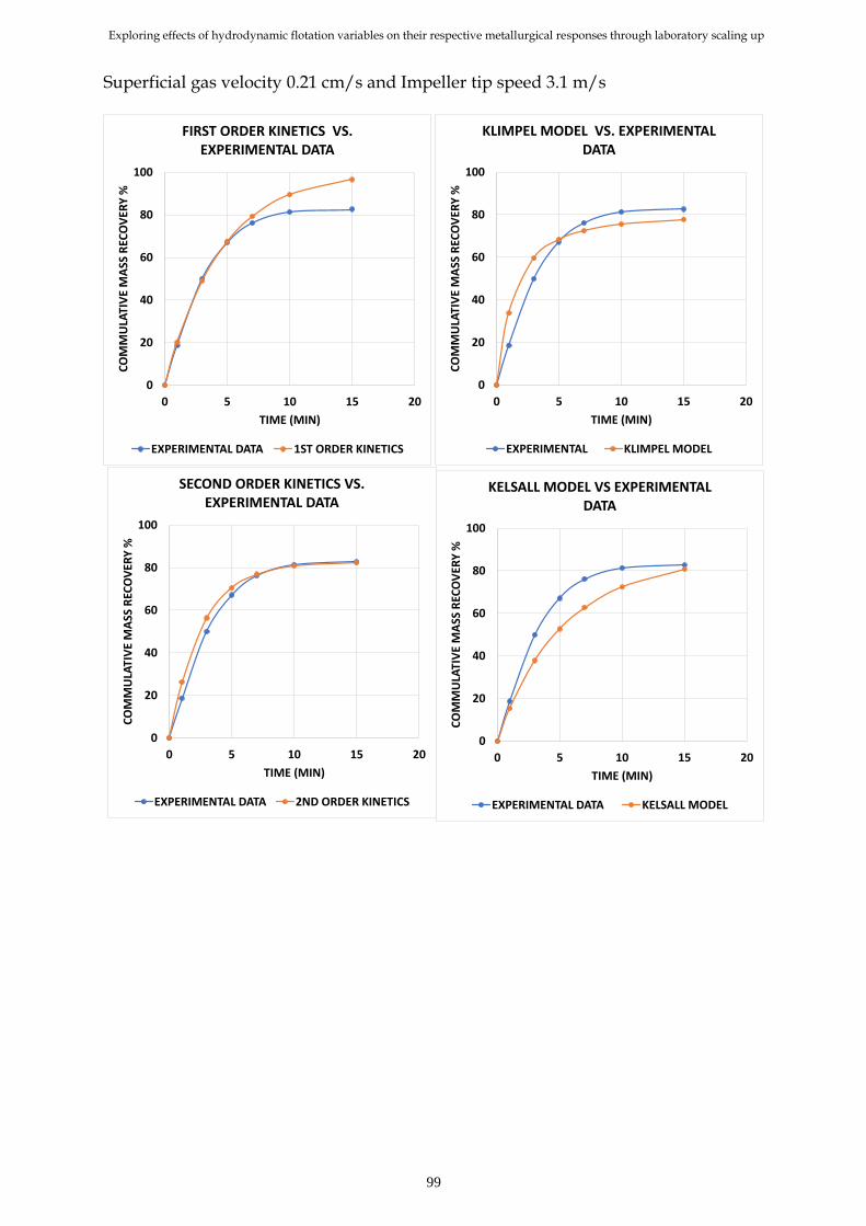
Exploring effects of hydrodynamic flotation variables on their respective metallurgical responses through laboratory scaling up
99
Superficial gas velocity 0.21 cm/s and Impeller tip speed 3.1 m/s
0
20
40
60
80
100
0 5 10 15 20
CO
MM
ULA
TIV
E M
ASS
REC
OV
ERY
%
TIME (MIN)
FIRST ORDER KINETICS VS. EXPERIMENTAL DATA
EXPERIMENTAL DATA 1ST ORDER KINETICS
0
20
40
60
80
100
0 5 10 15 20
CO
MM
ULA
TIV
E M
ASS
REC
OV
ERY
%
TIME (MIN)
SECOND ORDER KINETICS VS. EXPERIMENTAL DATA
EXPERIMENTAL DATA 2ND ORDER KINETICS
0
20
40
60
80
100
0 5 10 15 20
CO
MM
ULA
TIV
E M
ASS
REC
OV
ERY
%
TIME (MIN)
KELSALL MODEL VS EXPERIMENTAL DATA
EXPERIMENTAL DATA KELSALL MODEL
0
20
40
60
80
100
0 5 10 15 20
CO
MM
ULA
TIV
E M
ASS
REC
OV
ERY
%
TIME (MIN)
KLIMPEL MODEL VS. EXPERIMENTAL DATA
EXPERIMENTAL KLIMPEL MODEL

Exploring effects of hydrodynamic flotation variables on their respective metallurgical responses through laboratory scaling up
100
Superficial gas velocity 0.14 cm/s and Impeller tip speed 3.1 m/s
0
20
40
60
80
100
0 5 10 15 20
CO
MM
ULA
TIV
E M
ASS
REC
OV
ERY
%
TIME (MIN)
FIRST ORDER KINETICS VS. EXPERIMENTAL DATA
EXPERIMENTAL DATA 1ST ORDER KINETICS
0
20
40
60
80
100
0 5 10 15 20
CO
MM
ULA
TIV
E M
ASS
REC
OV
ERY
%
TIME (MIN)
SECOND ORDER KINETICS VS. EXPERIMENTAL DATA
EXPERIMENTAL DATA 2ND ORDER KINETICS
0
20
40
60
80
100
0 5 10 15 20
CO
MM
ULA
TIV
E M
ASS
REC
OV
ERY
%
TIME (MIN)
KELSALL MODEL VS EXPERIMENTAL DATA
EXPERIMENTAL DATA KELSALL MODEL
0
20
40
60
80
100
0 5 10 15 20
CO
MM
ULA
TIV
E M
ASS
REC
OV
ERY
%
TIME (MIN)
KLIMPEL MODEL VS. EXPERIMENTAL DATA
EXPERIMENTAL KLIMPEL MODEL