Embed Size (px)
Citation preview
Experimental studies of
a low emittance electron beam
in the KEK-ATF damping ring
with a laserwire beam profile monitor
by
Yosuke HONDA
A Dissertation
Department of Physics, Faculty of Science,
Kyoto University
July 28, 2004

Abstract
Production of a low-emittance beam is one of the key technologies in realizing the
future linear colliders. The Accelerator Test Facility at KEK has been built to establish
technologies to generate the required low-emittance beam, and to experimentally study
the effects which might limit emittance reduction.
A beam monitor called the laserwire beam profile monitor was developed to measure
the emittance of a stored beam in the ATF damping ring. This monitor has been up-
graded to enable faster measurements of both transverse beam sizes with a better spatial
resolution. The signal detection scheme was also modified to separately measure the beam
profiles of each bunch in a multi-bunch beam.
Continuous efforts have been made to reduce emittances further, and intensive stud-
ies have been done with the upgraded laserwire monitor. Four-dimensional beam sizes
and their intensity dependence were measured in various bunch volume conditions. In
particular, it was found that the vertical emittance of a single-bunch mode was reduced
to 4 pm·rad in the zero current limit, the smallest emittance ever achieved in the world,
and it grow by about factor of 1.5 at the intensity of 1010 electrons per bunch. The over-
all nature of two transverse emittances, bunch length, and momentum spread seemed to
have no serious disagreement with the expectation of the model calculation involving the
intra-beam scattering.
The emittance was also measured in the multi-bunch operational mode. It was found
that the generation of a similar small emittance was possible to those realized in a single-
bunch mode. No large bunch-to-bunch difference was seen in the beam intensity studied
so far. All the results above, obtained with the laserwire monitor, have proved to be an
important milestone for realizing future linear colliders.
Acknowledgments
This thesis could not have been written without the help and support of many people.
Firstly, I would like to express my gratitude to my supervisor Prof. N. Sasao of Kyoto
University and Prof. J. Urakawa of High Energy Accelerator Research Organization
(KEK).
I am particularly grateful to the members of the laserwire development group: Prof.
Y. Higashi, T. Taniguchi, T. Okugi, S. Araki, M. Takano, M. Nomura, K. Hirano, Y.
Yamazaki, H. Sakai and K. Takezawa, for their generous help and suggestions through all
the work.
I would like to express my gratitude to all the members of KEK-ATF: Prof. H. Hayano,
K. Kubo, N. Terunuma, S. Kuroda, M. Kuriki, T. Naito, Prof. N. Toge, Prof. S. Kamada,
Prof. Higo, Prof. T. Suzuki, Prof. K. Nakajima, Prof. T. Tauchi, T. Omori, Y. Kurihara,
N. Kudo, T. Saeki, V. Vogel, N. Delerue, H. Sasaki, people from E-cube co. and Kanto-
Joho co.. Witout their hard work to develop and operate the ATF, this study never be
accomplished.
I would like to acknowledge to all the students worked together at ATF: K. Dobashi, T.
Imai, I. Sakai, T. Muto, M. Fukuda, R. Kuroda, P. Karataev, A. Higurashi, K. Hasegawa,
A. Aoki, T. Oshima, T. Iimura, K. Iida, T. Hirose, Y. Inoue, A. Ohashi, I. Yamazaki, M.
Matsuda, K. Watanabe, T. Suehara, H. Fujimoto and others.
I am grateful to collabolators from other facilities: M. Ross, J. Frisch, D. McCormick,
M. Woodley, J. Nelson, J. Turner, T. Raubenheimer, A. Wolski, F. Zimmermann, G.
Blair, T. Kamps and others. Fruitful discussions with them helped us a lot.
Last but not least, I would like thank to the members of High Energy Physics group of
Kyoto university: Prof. K. Nishikawa, Prof. H. Sakamoto, Prof. T. Nakaya, R. Kikuchi,
T. Nomura, M. Yokoyama, M. Suehiro, Y. Takeuchi, K. Murakami, Y. Ushiroda, T.
Inagaki, T. Fujiwara, T. Nakamura, N. Nakamura, T. Shima, S. Nishida, H. Yokoyama, H.
Yumura, S. Mukai, I. Kato, A. Shima, E. Shinya, H. Maesaka, K. Mizouchi, K. Uchida, M.
Hasegawa, S. Yamamoto, T. Sumida, S. Tsuji, T. Sasaki, H. Morii, S. Ueda, K. Hayashi,
T. Morita, J. Kubota, T. Shirai, N. Taniguchi, K. Hiraide, and others. I am thankful to
the secretary of our group T. Ishino and A. Nakao and the secretariat members of the
physics department, K. Nakagawa, A. Saito and A. Nishino. I have been staying in KEK,
but always been supported by all of them.
Kyoto, Japan
August 15, 2004.
Yosuke HONDA
Contents
1 Introduction 1
1.1 Linear Colliders . . . . . . . . . . . . . . . . . . . . . . . . . . . . . . . . . 1
1.2 Low emittance beams and the ATF . . . . . . . . . . . . . . . . . . . . . . 2
1.3 Laser-based beam diagnostics . . . . . . . . . . . . . . . . . . . . . . . . . 5
2 The KEK Accelerator Test Facility 7
2.1 Overview of the accelerator complex . . . . . . . . . . . . . . . . . . . . . 7
2.1.1 Electron-gun system . . . . . . . . . . . . . . . . . . . . . . . . . . 7
2.1.2 Linac . . . . . . . . . . . . . . . . . . . . . . . . . . . . . . . . . . . 10
2.1.3 Damping ring . . . . . . . . . . . . . . . . . . . . . . . . . . . . . . 10
2.1.4 Extraction line . . . . . . . . . . . . . . . . . . . . . . . . . . . . . 13
2.2 Instrumentation . . . . . . . . . . . . . . . . . . . . . . . . . . . . . . . . . 13
2.2.1 Measurement of beam intensity . . . . . . . . . . . . . . . . . . . . 13
2.2.2 Beam position monitor . . . . . . . . . . . . . . . . . . . . . . . . . 14
2.2.3 Beam exciter and the measurement of the betatron tune . . . . . . 16
2.2.4 Momentum spread monitor . . . . . . . . . . . . . . . . . . . . . . 17
2.2.5 Streak camera . . . . . . . . . . . . . . . . . . . . . . . . . . . . . . 17
2.2.6 Beam profile monitors . . . . . . . . . . . . . . . . . . . . . . . . . 19
2.3 Production of a low emittance beam . . . . . . . . . . . . . . . . . . . . . 20
2.3.1 Sources of the vertical emittance growth . . . . . . . . . . . . . . . 20
2.3.2 Precise alignment of the accelerator components . . . . . . . . . . . 21
2.3.3 Beam tuning . . . . . . . . . . . . . . . . . . . . . . . . . . . . . . 23
3 Laserwire Beam Profile Monitor 28
3.1 Principle of the laserwire monitor . . . . . . . . . . . . . . . . . . . . . . . 28
3.1.1 Principle of the measurement . . . . . . . . . . . . . . . . . . . . . 28
3.1.2 Compton scattering . . . . . . . . . . . . . . . . . . . . . . . . . . . 28
3.1.3 Estimation of the count rate . . . . . . . . . . . . . . . . . . . . . . 31
3.2 Optical cavity . . . . . . . . . . . . . . . . . . . . . . . . . . . . . . . . . . 33
3.2.1 Principle of the power enhancement . . . . . . . . . . . . . . . . . . 34
3.2.2 Properties of a laser beam . . . . . . . . . . . . . . . . . . . . . . . 36
3.3 Experimental setup . . . . . . . . . . . . . . . . . . . . . . . . . . . . . . . 39
3.3.1 Layout . . . . . . . . . . . . . . . . . . . . . . . . . . . . . . . . . . 39
3.3.2 Optical system . . . . . . . . . . . . . . . . . . . . . . . . . . . . . 39
3.3.3 Properties of the optical cavities and their control . . . . . . . . . . 42
- i -

3.3.4 Photon detector and collimators . . . . . . . . . . . . . . . . . . . . 45
3.3.5 Readout circuits . . . . . . . . . . . . . . . . . . . . . . . . . . . . . 49
3.3.6 Data processing . . . . . . . . . . . . . . . . . . . . . . . . . . . . . 49
3.3.7 Setup procedure of the detector system . . . . . . . . . . . . . . . . 50
3.3.8 Scanning and data taking system . . . . . . . . . . . . . . . . . . . 50
3.4 Measurement of the beam waist . . . . . . . . . . . . . . . . . . . . . . . . 50
3.4.1 Beam divergence method . . . . . . . . . . . . . . . . . . . . . . . . 54
3.4.2 Transverse mode difference method . . . . . . . . . . . . . . . . . . 56
3.4.3 Waist scan by an electron beam . . . . . . . . . . . . . . . . . . . . 56
3.4.4 Summary of the beam waist measurement . . . . . . . . . . . . . . 58
4 Experiments with a Single-Bunch Beam 61
4.1 Introduction . . . . . . . . . . . . . . . . . . . . . . . . . . . . . . . . . . . 61
4.1.1 Emittance measurements prior to this experiment . . . . . . . . . . 61
4.1.2 Improvements to the ATF damping ring . . . . . . . . . . . . . . . 62
4.2 Procedure of the experiment . . . . . . . . . . . . . . . . . . . . . . . . . . 64
4.2.1 Beam tuning and damping ring conditions . . . . . . . . . . . . . . 64
4.2.2 Measurements of transverse beam profiles . . . . . . . . . . . . . . 65
4.2.3 Measurement of dispersion function at the collision points of laserwires 68
4.2.4 Measurement of the beta function . . . . . . . . . . . . . . . . . . 73
4.2.5 Estimation of the transverse emittances . . . . . . . . . . . . . . . 75
4.2.6 Measurement of the bunch length . . . . . . . . . . . . . . . . . . . 76
4.2.7 Measurement of the momentum spread . . . . . . . . . . . . . . . 80
4.3 Results . . . . . . . . . . . . . . . . . . . . . . . . . . . . . . . . . . . . . . 80
4.3.1 Transverse emittances . . . . . . . . . . . . . . . . . . . . . . . . . 81
4.3.2 Bunch length . . . . . . . . . . . . . . . . . . . . . . . . . . . . . . 82
4.3.3 Momentum spread . . . . . . . . . . . . . . . . . . . . . . . . . . . 82
4.4 Discussion . . . . . . . . . . . . . . . . . . . . . . . . . . . . . . . . . . . . 82
4.4.1 Estimation of the impedance effect . . . . . . . . . . . . . . . . . . 84
4.4.2 Simulation of the emittance and the momentum spread . . . . . . . 86
4.4.3 Comparison with the calculation . . . . . . . . . . . . . . . . . . . . 86
4.5 Summary . . . . . . . . . . . . . . . . . . . . . . . . . . . . . . . . . . . . 88
5 Experiments with a Multi-Bunch Beam 91
5.1 Introduction . . . . . . . . . . . . . . . . . . . . . . . . . . . . . . . . . . . 91
5.2 Laserwire monitor for multi-bunch beam measurement . . . . . . . . . . . 92
5.2.1 Data taking system . . . . . . . . . . . . . . . . . . . . . . . . . . . 92
5.2.2 Analysis procedure . . . . . . . . . . . . . . . . . . . . . . . . . . . 95
5.3 First systematic emittance measurement (Run 1) . . . . . . . . . . . . . . 95
5.3.1 Results . . . . . . . . . . . . . . . . . . . . . . . . . . . . . . . . . . 96
5.3.2 Discussions and Summary . . . . . . . . . . . . . . . . . . . . . . . 100
5.4 Comparison between the single and multi-bunch modes (Run 2 and 3) . . . 100
5.4.1 Result . . . . . . . . . . . . . . . . . . . . . . . . . . . . . . . . . . 101
5.4.2 Discussions and Summary . . . . . . . . . . . . . . . . . . . . . . . 102
- ii -

5.5 Pressure dependence study (Run 4) . . . . . . . . . . . . . . . . . . . . . . 102
5.5.1 Data taking . . . . . . . . . . . . . . . . . . . . . . . . . . . . . . . 103
5.5.2 Result . . . . . . . . . . . . . . . . . . . . . . . . . . . . . . . . . . 103
5.5.3 Discussion and Summary . . . . . . . . . . . . . . . . . . . . . . . . 103
6 Conclusion 107
A Beam Dynamics 110
A.1 Linear beam dynamics in a circular accelerator . . . . . . . . . . . . . . . . 110
A.1.1 Betatron motion . . . . . . . . . . . . . . . . . . . . . . . . . . . . 110
A.1.2 Radiation damping . . . . . . . . . . . . . . . . . . . . . . . . . . . 112
A.1.3 Quantum excitation and equilibrium . . . . . . . . . . . . . . . . . 114
A.2 Intra-beam Scattering . . . . . . . . . . . . . . . . . . . . . . . . . . . . . 115
A.2.1 Touschek effect . . . . . . . . . . . . . . . . . . . . . . . . . . . . . 115
A.2.2 Intra-beam scattering . . . . . . . . . . . . . . . . . . . . . . . . . . 116
A.3 Fast Beam-Ion Instability . . . . . . . . . . . . . . . . . . . . . . . . . . . 116
A.3.1 Equations of motion . . . . . . . . . . . . . . . . . . . . . . . . . . 116
A.3.2 Solution . . . . . . . . . . . . . . . . . . . . . . . . . . . . . . . . . 117
B Laserwire Monitor Utilizing a Higher Order Mode 118
B.1 An idea of utilizing the higher order mode . . . . . . . . . . . . . . . . . . 118
B.1.1 Diffraction limit . . . . . . . . . . . . . . . . . . . . . . . . . . . . . 118
B.1.2 Higher order modes of an optical cavity . . . . . . . . . . . . . . . . 119
B.1.3 Principle of the beam size measurement with a TEM01 laserwire . . 119
B.2 Realization of the TEM01 mode resonance . . . . . . . . . . . . . . . . . . 121
B.2.1 Mode splitting of TEM01 and TEM10 mode . . . . . . . . . . . . . . 121
B.2.2 Excitation of higher order modes . . . . . . . . . . . . . . . . . . . 122
B.3 Measurement of an electron beam size . . . . . . . . . . . . . . . . . . . . 124
B.3.1 Data taking . . . . . . . . . . . . . . . . . . . . . . . . . . . . . . . 124
B.3.2 Analysis and Result . . . . . . . . . . . . . . . . . . . . . . . . . . . 126
B.4 Summary . . . . . . . . . . . . . . . . . . . . . . . . . . . . . . . . . . . . 126
C Latest Results of the Multi-Bunch Measurement 129
C.1 Change in the laserwire setup . . . . . . . . . . . . . . . . . . . . . . . . . 129
C.2 Data taking . . . . . . . . . . . . . . . . . . . . . . . . . . . . . . . . . . . 129
C.3 Results and discussion . . . . . . . . . . . . . . . . . . . . . . . . . . . . . 130
- iii -

List of Figures
1.1 Schematic layout of GLC. . . . . . . . . . . . . . . . . . . . . . . . . . . . 2
1.2 Hadronic annihilation cross section in e+e− collisions. . . . . . . . . . . . . 3
1.3 Normalized emittance of two directions for various rings. . . . . . . . . . . 5
2.1 Layout of the Accelerator Test Facility. . . . . . . . . . . . . . . . . . . . . 8
2.2 Schematic figure of a photo-cathode RF-gun. . . . . . . . . . . . . . . . . . 9
2.3 Laser system for the RF-gun. . . . . . . . . . . . . . . . . . . . . . . . . . 9
2.4 Regular RF unit. . . . . . . . . . . . . . . . . . . . . . . . . . . . . . . . . 10
2.5 Principle of the energy compensation system. . . . . . . . . . . . . . . . . 10
2.6 Optical functions of the entire damping ring. . . . . . . . . . . . . . . . . . 12
2.7 Lattice functions of the normal cell. . . . . . . . . . . . . . . . . . . . . . . 13
2.8 Layout of the extraction line. . . . . . . . . . . . . . . . . . . . . . . . . . 14
2.9 Principle of the DCCT monitor. . . . . . . . . . . . . . . . . . . . . . . . . 15
2.10 Principle of the wall current monitor. . . . . . . . . . . . . . . . . . . . . . 15
2.11 Schematics of the button type beam position monitor. . . . . . . . . . . . . 16
2.12 Principle of the beam exciter. . . . . . . . . . . . . . . . . . . . . . . . . . 17
2.13 Momentum spread monitor (screen monitor). . . . . . . . . . . . . . . . . . 18
2.14 Schematics of the streak camera. . . . . . . . . . . . . . . . . . . . . . . . 18
2.15 Various misalignments of the magnets. . . . . . . . . . . . . . . . . . . . . 21
2.16 Transverse positioning of the magnets. . . . . . . . . . . . . . . . . . . . . 22
2.17 Longitudinal positioning of the magnets. . . . . . . . . . . . . . . . . . . . 22
2.18 Principle of the beam based alignment. . . . . . . . . . . . . . . . . . . . . 22
2.19 Example of the dispersion measurement. . . . . . . . . . . . . . . . . . . . 23
2.20 Example of the coupling measurement. . . . . . . . . . . . . . . . . . . . . 24
2.21 Skew winding of the sextupole magnets. . . . . . . . . . . . . . . . . . . . 25
2.22 Simulation results for the vertical emittance. . . . . . . . . . . . . . . . . . 27
3.1 Principle of the beam size measurement by the laserwire. . . . . . . . . . . 29
3.2 Compton scattering in the electron rest frame. . . . . . . . . . . . . . . . . 30
3.3 Lorentz transformation from the electron rest frame to the laboratory frame. 31
3.4 Energy spectrum of the Compton scattered photon. . . . . . . . . . . . . . 32
3.5 The energy of the scattered photon vs the scattering angle. . . . . . . . . . 32
3.6 Differential cross section vs the scattered angle. . . . . . . . . . . . . . . . 32
3.7 Integrated cross section within a given aperture. . . . . . . . . . . . . . . . 32
3.8 Schematic view of the laserwires interacting with the electron beam. . . . . 34
- iv -

3.9 Schematic diagram of the power enhancement in an optical cavity. . . . . . 35
3.10 Resonance efficiency (η) as a function of phase advance (θ). . . . . . . . . . 37
3.11 Cavity response near the resonance condition. . . . . . . . . . . . . . . . . 37
3.12 Pattern of the field allowed to exist in an optical cavity. . . . . . . . . . . . 38
3.13 Resonance conditions of various transverse modes. . . . . . . . . . . . . . . 39
3.14 Layout of the laserwire setup. . . . . . . . . . . . . . . . . . . . . . . . . . 40
3.15 Cavity assembly and vacuum chamber. . . . . . . . . . . . . . . . . . . . . 41
3.16 Chamber system of the laserwire. . . . . . . . . . . . . . . . . . . . . . . . 41
3.17 Bird’s view of the laserwire vacuum chambers and the laser beam transport. 43
3.18 Layout of the optical components. . . . . . . . . . . . . . . . . . . . . . . . 43
3.19 Mode matching procedure of the laser beam and the cavity. . . . . . . . . . 44
3.20 Geometry of the cavity mirror. . . . . . . . . . . . . . . . . . . . . . . . . . 44
3.21 Schematics of the feedback circuit. . . . . . . . . . . . . . . . . . . . . . . 46
3.22 The transmittance signal from the cavity (ch1) and the comparator outputs
(ch2 and ch3). . . . . . . . . . . . . . . . . . . . . . . . . . . . . . . . . . . 46
3.23 Photon detector setup. . . . . . . . . . . . . . . . . . . . . . . . . . . . . . 47
3.24 Simulation results of the detector responses to the Compton scattered pho-
tons. . . . . . . . . . . . . . . . . . . . . . . . . . . . . . . . . . . . . . . . 47
3.25 Calibration of the detector. . . . . . . . . . . . . . . . . . . . . . . . . . . 48
3.26 Energy spectrum of the background events. . . . . . . . . . . . . . . . . . . 48
3.27 Schematic diagram of the readout circuits. . . . . . . . . . . . . . . . . . . 49
3.28 Alignment of the collimator system (step 1). . . . . . . . . . . . . . . . . . 51
3.29 Alignment of the collimator system (step 2). . . . . . . . . . . . . . . . . . 51
3.30 Alignment of the collimator system (step 3). . . . . . . . . . . . . . . . . . 51
3.31 Alignment of the collimator system (step 4). . . . . . . . . . . . . . . . . . 51
3.32 Count rates vs the beam current (on beam). . . . . . . . . . . . . . . . . . 52
3.33 Count rates vs the beam current (off beam). . . . . . . . . . . . . . . . . . 52
3.34 Energy spectrum of the signal and background. . . . . . . . . . . . . . . . 53
3.35 Schematic of the beam divergence method. . . . . . . . . . . . . . . . . . . 55
3.36 Results of the beam divergence method (h-wire). . . . . . . . . . . . . . . . 55
3.37 Results of the beam divergence method (v-wire). . . . . . . . . . . . . . . . 55
3.38 Waist measurement by the transverse modes. . . . . . . . . . . . . . . . . . 57
3.39 The beam waist (w0) vs ∆Lλ/2
. . . . . . . . . . . . . . . . . . . . . . . . . . . 57
3.40 Resonance structure observed in the transmittance signal of the sweep mode. 57
3.41 Results of the beam waist scan. . . . . . . . . . . . . . . . . . . . . . . . . 59
3.42 Fitting result of σe and w0/2. . . . . . . . . . . . . . . . . . . . . . . . . . 59
3.43 Comparison of the beam waist measurements by three methods. . . . . . . 60
4.1 Single bunch emittance data of the 2000-2001 runs. . . . . . . . . . . . . . 63
4.2 Example of the scan procedure (low intensity case) . . . . . . . . . . . . . 66
4.3 Example of the scan procedure (high current case) . . . . . . . . . . . . . . 66
4.4 Example of the measured profile and the fit result (vertical scan). . . . . . 67
4.5 Example of the measured profile and the fit result (horizontal scan). . . . . 67
4.6 Example of the dispersion measurement. . . . . . . . . . . . . . . . . . . . 72
- v -
4.7 Layout of the quadrupole magnets in the neighborhood of the laserwire. . . 73
4.8 Tune shift vs the quadrupole strength. . . . . . . . . . . . . . . . . . . . . 74
4.9 Example of the beta function measurement. . . . . . . . . . . . . . . . . . 75
4.10 Current dependence of emittances (run A). . . . . . . . . . . . . . . . . . . 77
4.11 Current dependence of emittances (run B). . . . . . . . . . . . . . . . . . . 77
4.12 Current dependence of emittances (run C). . . . . . . . . . . . . . . . . . . 77
4.13 Current dependence of emittances (run D). . . . . . . . . . . . . . . . . . . 78
4.14 Current dependence of emittances (run E). . . . . . . . . . . . . . . . . . . 78
4.15 Current dependence of emittances (run F). . . . . . . . . . . . . . . . . . . 78
4.16 Example of the bunch length measurement by the streak camera. . . . . . 79
4.17 Example of the calibration measurement by the streak camera. . . . . . . . 79
4.18 Current dependence of the bunch length. . . . . . . . . . . . . . . . . . . . 80
4.19 Current dependence of the momentum spread. . . . . . . . . . . . . . . . . 81
4.20 Simple model for the longitudinal bunch shape. . . . . . . . . . . . . . . . 85
4.21 Fit result for Vc as a function of N/σ3z . . . . . . . . . . . . . . . . . . . . . 86
4.22 Simulation result for the emittance and the momentum spread (0.4% cou-
pling) . . . . . . . . . . . . . . . . . . . . . . . . . . . . . . . . . . . . . . 87
4.23 Simulation result for the emittance and the momentum spread (3% coupling) 87
4.24 Simulation result for the emittance and the momentum spread (6% coupling) 87
4.25 Correlation between ε(0)y and r(10)εy
. . . . . . . . . . . . . . . . . . . . . . . . 89
4.26 Correlation between ε(0)y and r(10)εx
. . . . . . . . . . . . . . . . . . . . . . . . 89
4.27 Correlation between ε(0)y and r(10)∆p/p. . . . . . . . . . . . . . . . . . . . . . . 89
4.28 Correlation between ε(0)y and the ε(0)x . . . . . . . . . . . . . . . . . . . . . . 90
4.29 Correlation between ε(0)y and ∆p/p(0). . . . . . . . . . . . . . . . . . . . . . 90
5.1 Schematic diagram of the readout circuits for the multi-bunch experiment. 93
5.2 Estimation of the timing resolution. . . . . . . . . . . . . . . . . . . . . . . 93
5.3 Performance of the modified circuits for the multi-bunch measurement. . . 94
5.4 Example of the combined profile of the multi-bunch beam. . . . . . . . . . 95
5.5 Bunch dependence of the 20-bunch beam (vertical, 18.8mA). . . . . . . . . 97
5.6 Bunch dependence of the 20-bunch beam (vertical, 9.8mA). . . . . . . . . . 97
5.7 Bunch dependence of the 20-bunch beam (vertical, 4.8mA). . . . . . . . . . 97
5.8 Bunch dependence of the 20-bunch beam (vertical, 1.7mA). . . . . . . . . . 97
5.9 Bunch dependence of the 20-bunch beam (horizontal, 18.4mA). . . . . . . . 98
5.10 Bunch dependence of the 20-bunch beam (horizontal, 8.5mA). . . . . . . . 98
5.11 Bunch dependence of the 20-bunch beam (horizontal,, 4.2mA). . . . . . . . 98
5.12 Bunch dependence of the 20-bunch beam (horizontal, 1.9mA). . . . . . . . 98
5.13 Vertical emittance of the 20-bunch beam vs the electron current. . . . . . . 100
5.14 Horizontal emittance of the 20-bunch beam vs the electron current. . . . . 100
5.15 Vertical beam size of the multi-bunch and single-bunch mode. . . . . . . . 102
5.16 Beam profile for each bunch (normal pressure). . . . . . . . . . . . . . . . . 104
5.17 Beam profile for each bunch (increased pressure). . . . . . . . . . . . . . . 104
5.18 Bunch dependence (normal pressure, 9.1 mA) . . . . . . . . . . . . . . . . 105
5.19 Bunch dependence (normal pressure, 6.5 mA) . . . . . . . . . . . . . . . . 105
- vi -

5.20 Bunch dependence (one arc, 10.1 mA, 5.0 × 10⁻⁶Pa) . . . . . . . . . . . . . 105
5.21 Bunch dependence (one arc, 6.7 mA, 4.0 × 10⁻⁶Pa) . . . . . . . . . . . . . 105
5.22 Bunch dependence (both arc, 7.9 mA, 6.0 × 10⁻⁶Pa) . . . . . . . . . . . . 105
5.23 Bunch dependence (both arc, 5.2 mA, 5.6 × 10⁻⁶Pa) . . . . . . . . . . . . 105
6.1 Normalized emittance of two transverse directions measured in our exper-
iment. . . . . . . . . . . . . . . . . . . . . . . . . . . . . . . . . . . . . . . 109
A.1 Coordinate system . . . . . . . . . . . . . . . . . . . . . . . . . . . . . . . 110
A.2 Trace of a particle in the phase space. . . . . . . . . . . . . . . . . . . . . . 112
A.3 Particle distribution in a phase space. . . . . . . . . . . . . . . . . . . . . . 112
A.4 Variation of accelerating voltage in an RF cavity as a function of electron
arrival time. . . . . . . . . . . . . . . . . . . . . . . . . . . . . . . . . . . 113
A.5 Emission of an synchrotron radiation and the acceleration in the cavity. . . 113
A.6 Coulomb scattering of two particles inside a bunch. . . . . . . . . . . . . . 115
A.7 Schematic diagram for the explanation of fast beam ion instability. . . . . 116
B.1 Schematic diagram for the explanation of the diffraction effect. . . . . . . . 119
B.2 Transverse profile of several modes. . . . . . . . . . . . . . . . . . . . . . . 120
B.3 Projected intensity distribution along the y direction of TEM00 and TEM01.120
B.4 Expected signal profiles scanned by the TEM01 mode laserwire. . . . . . . 121
B.5 Sensitivity of the TEM01 mode measurement. . . . . . . . . . . . . . . . . 121
B.6 Structure of the mirror holder. . . . . . . . . . . . . . . . . . . . . . . . . . 122
B.7 Mirror distortion measurement. . . . . . . . . . . . . . . . . . . . . . . . . 123
B.8 Higher mode excitation by injection axis shift. . . . . . . . . . . . . . . . . 124
B.9 Higher mode excitation by mode converter. . . . . . . . . . . . . . . . . . . 125
B.10 Measured profiles by the TEM01 mode laserwire. . . . . . . . . . . . . . . . 127
B.11 Results of σlw and σe by the TEM01 mode laserwire. . . . . . . . . . . . . . 128
C.1 Results of the single-train multi-bunch beam. . . . . . . . . . . . . . . . . 131
C.2 Results of the three-train multi-bunch beam. . . . . . . . . . . . . . . . . 131
- vii -

List of Tables
1.1 Design parameters of GLC. . . . . . . . . . . . . . . . . . . . . . . . . . . 3
2.1 Parameters of the ATF damping ring. . . . . . . . . . . . . . . . . . . . . . 11
2.2 Random errors applied to the magnets in the simulation. . . . . . . . . . . 26
3.1 Specifications of the optical cavities. . . . . . . . . . . . . . . . . . . . . . . 45
3.2 Summary of the w0 measurement by the divergence method. . . . . . . . . 54
3.3 Summary of the w0 measurements by the transverse mode method . . . . . 58
4.1 List of ring conditions for runs A∼F . . . . . . . . . . . . . . . . . . . . . 64
4.2 Scan list (run A). . . . . . . . . . . . . . . . . . . . . . . . . . . . . . . . . 68
4.3 Scan list (run B). . . . . . . . . . . . . . . . . . . . . . . . . . . . . . . . . 69
4.4 Scan list (run C). . . . . . . . . . . . . . . . . . . . . . . . . . . . . . . . . 70
4.5 Scan list (run D). . . . . . . . . . . . . . . . . . . . . . . . . . . . . . . . . 70
4.6 Scan list (run E). . . . . . . . . . . . . . . . . . . . . . . . . . . . . . . . . 71
4.7 Scan list (run F) . . . . . . . . . . . . . . . . . . . . . . . . . . . . . . . . 71
4.8 Summary of the dispersion measurement . . . . . . . . . . . . . . . . . . . 72
4.9 Summary of the tune measurement . . . . . . . . . . . . . . . . . . . . . . 73
4.10 Results of the beta function measurement at quadrupole magnets. . . . . . 74
4.11 Results of the beta function measurement at the laserwire. . . . . . . . . . 75
4.12 Results of fitting analysis (emittance). . . . . . . . . . . . . . . . . . . . . 83
4.13 Results of fitting analysis (bunch length). . . . . . . . . . . . . . . . . . . . 84
4.14 Results of fitting analysis (momentum spread). . . . . . . . . . . . . . . . . 84
4.15 Simulation results of the current dependence. . . . . . . . . . . . . . . . . . 88
5.1 Experiments with a multi-bunch beam. . . . . . . . . . . . . . . . . . . . . 91
5.2 Summary of bunch-dependence of the beam width σmeas measurements in
the multi-bunch mode. . . . . . . . . . . . . . . . . . . . . . . . . . . . . . 96
5.3 Results of the combined analysis (vertical). . . . . . . . . . . . . . . . . . . 99
5.4 Results of the combined analysis (horizontal). . . . . . . . . . . . . . . . . 99
5.5 Results of the beta function and dispersion measurements. . . . . . . . . . 99
5.6 Results of the combined multi-bunch beam size measurements (run 2).. . . 101
5.7 Results of the single-bunch beam size measurements (run 3). . . . . . . . . 101
B.1 List of the beam and laser conditions. . . . . . . . . . . . . . . . . . . . . . 125
B.2 Results of the measurements by the TEM01 mode laserwire. . . . . . . . . 126
- viii -

C.1 List of beam conditions. . . . . . . . . . . . . . . . . . . . . . . . . . . . . 130
- ix -
Chapter 1. Introduction
Chapter 1
Introduction
1.1 Linear Colliders
Quests for the fundamental constituents of matter and the law which governs everything
in the universe, have always been a frontier of human activities. In elementary particle
physics, accelerators have played an important role in pioneering this profound field of
knowledge. Experiments with accelerated particle beams have discovered hundreds of new
particles and revealed the underlying principles of the dynamics.
The energy frontier has been explored by two types of high energy colliding beams:
hadron (proton and anti-proton) and lepton (electron and positron) beam. The former
has an advantage in discovering a signal of new particles and/or new phenomena. This is
due to the versatile nature of the beam. On the other hand, thanks to its well-known and
clean nature, the latter plays a crucial role in establishing the precision properties. Up
to now, colliding beams have always employed a circular acceleration scheme because of
its efficiency. Among the electron-positron (e+e−) colliders, LEP-II, the largest circular
machine, has reached the highest center-of-mass (CM) energy of ∼200 GeV. This energy
in generally considered to be the limit of the e+e− circular machine due to its huge energy
loss by synchrotron radiations.
Future e+e− linear colliders are aiming to open up the energy region of TeV scale
employing a different scheme of acceleration. A number of linear collider projects have
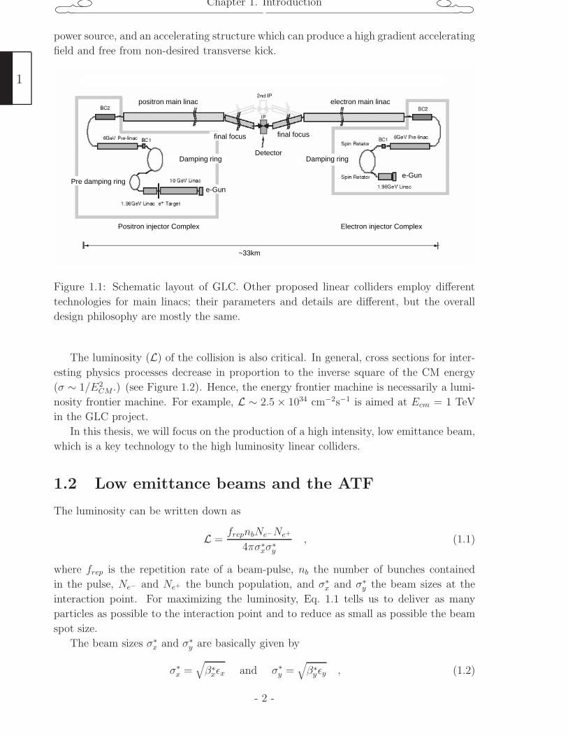
been proposed in the world, such as TESLA [1], NLC [2], GLC [3] and CLIC [4]. Figure 1.1
shows the conceptual design of GLC. Electron and positron beams are accelerated up to
∼500 GeV all the way through long linear accelerators, and then collisions are realized
in single crossing of two beams. Some important parameters of GLC are summarized in
Table 1.1.
There are two crucial technologies in realizing TeV-scale linear colliders: development
of a high-gradient accelerator and production of a low emittance beam. The former is
essential to reach a needed energy within a realistic length while the latter is crucial to
realize a luminosity required for physics.
As for the gradient issue, an effective acceleration gradient of more than 50 MV/m
is required, a challenging value compared to about 25 MV/m in existing linacs. Various
technologies and/or components have to be developed; for instance, a high-efficiency RF
- 1 -
1
Chapter 1. Introduction
power source, and an accelerating structure which can produce a high gradient accelerating
field and free from non-desired transverse kick.
positron main linac electron main linac
DetectorDamping ringDamping ring
Pre damping ring
~33km
final focus final focus
e-Gun
e-Gun
Positron injector Complex Electron injector Complex
Figure 1.1: Schematic layout of GLC. Other proposed linear colliders employ different
technologies for main linacs; their parameters and details are different, but the overall
design philosophy are mostly the same.
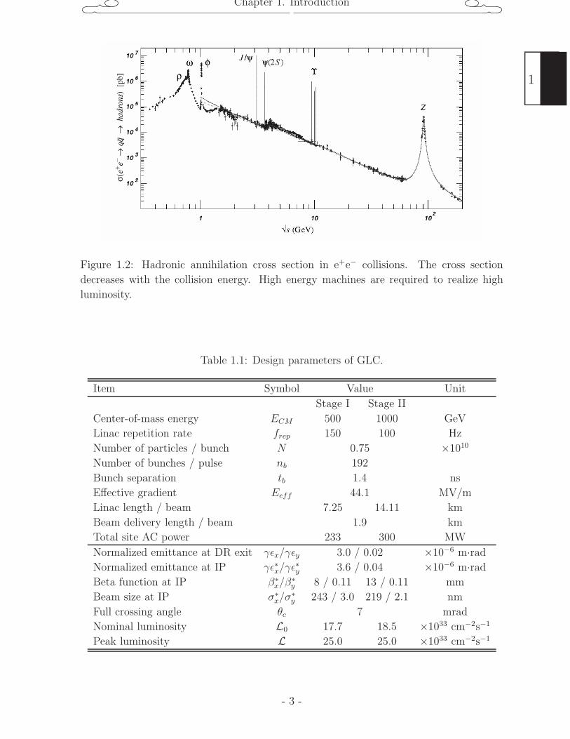
The luminosity (L) of the collision is also critical. In general, cross sections for inter-
esting physics processes decrease in proportion to the inverse square of the CM energy
(σ ∼ 1/E2CM .) (see Figure 1.2). Hence, the energy frontier machine is necessarily a lumi-
nosity frontier machine. For example, L ∼ 2.5 × 1034 cm−2s−1 is aimed at Ecm = 1 TeV
in the GLC project.
In this thesis, we will focus on the production of a high intensity, low emittance beam,
which is a key technology to the high luminosity linear colliders.
1.2 Low emittance beams and the ATF
The luminosity can be written down as
L =frepnbNe−Ne+
4πσ∗xσ
∗y
, (1.1)
where frep is the repetition rate of a beam-pulse, nb the number of bunches contained
in the pulse, Ne− and Ne+ the bunch population, and σ∗x and σ∗
y the beam sizes at the
interaction point. For maximizing the luminosity, Eq. 1.1 tells us to deliver as many
particles as possible to the interaction point and to reduce as small as possible the beam
spot size.
The beam sizes σ∗x and σ∗
y are basically given by
σ∗x =
√β∗
xεx and σ∗y =
√β∗
yεy , (1.2)
1
- 2 -
Chapter 1. Introduction
Figure 1.2: Hadronic annihilation cross section in e+e− collisions. The cross section
decreases with the collision energy. High energy machines are required to realize high
luminosity.
Table 1.1: Design parameters of GLC.
Item Symbol Value Unit
Stage I Stage II
Center-of-mass energy ECM 500 1000 GeV
Linac repetition rate frep 150 100 Hz
Number of particles / bunch N 0.75 ×10¹⁰
Number of bunches / pulse nb 192
Bunch separation tb 1.4 ns
Effective gradient Eeff 44.1 MV/m
Linac length / beam 7.25 14.11 km
Beam delivery length / beam 1.9 km
Total site AC power 233 300 MW
Normalized emittance at DR exit γεx/γεy 3.0 / 0.02 ×10⁻⁶ m·rad
Normalized emittance at IP γε∗x/γε∗y 3.6 / 0.04 ×10⁻⁶ m·rad
Beta function at IP β∗x/β
∗y 8 / 0.11 13 / 0.11 mm
Beam size at IP σ∗x/σ
∗y 243 / 3.0 219 / 2.1 nm
Full crossing angle θc 7 mrad
Nominal luminosity L0 17.7 18.5 ×1033 cm−2s−1
Peak luminosity L 25.0 25.0 ×1033 cm−2s−1
- 3 -
1
Chapter 1. Introduction
where β∗x(y) is the value of a horizontal (vertical) β function at the interaction point and
εx(y) is the horizontal (vertical) emittance. In general, β function can be controlled by
focusing elements. A strong quadrupole doublet will be used in the GLC final focus
system to obtain small β. We note that a precise chromaticity compensation scheme has
to be included in the final focus system [5]. This is because the spot size may be diluted
at the collision point due to the chromaticity arising from the strong focusing. Emittance
is a measure which represents the distribution of the particle’s transverse motion. Smaller
emittance means a more compact distribution in the phase space.
Apparently, production and handling of a low emittance beam is the key technology
to achieve the required luminosity. In any linear collider project, production of a low
emittance beam is realized in a special ring, called usually a damping ring. In these rings,
beam’s transverse motions are converted to longitudinal motions by a combination of
energy loss via synchrotron radiations and energy gain in an RF acceleration cavity (See
Appendix A in detail.). This cooling process in the transverse plane will compete with
a heating process due to a combination of quantum fluctuation of particle’s energy and
a dispersion function. Thus an equilibrium emittance is basically determined by ring’s
optical functions. Damping rings employ optical functions specially designed to achieve
small emittances. We note that since there is no bending magnet in a vertical plane
(the dispersion function is zero around the ring), an equilibrium emittance is very small,
usually determined by unavoidable x-y coupling due to magnet misalignments and/or field
errors. We also note that the discussion above is true only in the zero current limit; if the
bunch population is large, then collective effects such as an intra-beam scattering should
be taken into account. The collective effects are the topics we like to study in this thesis.
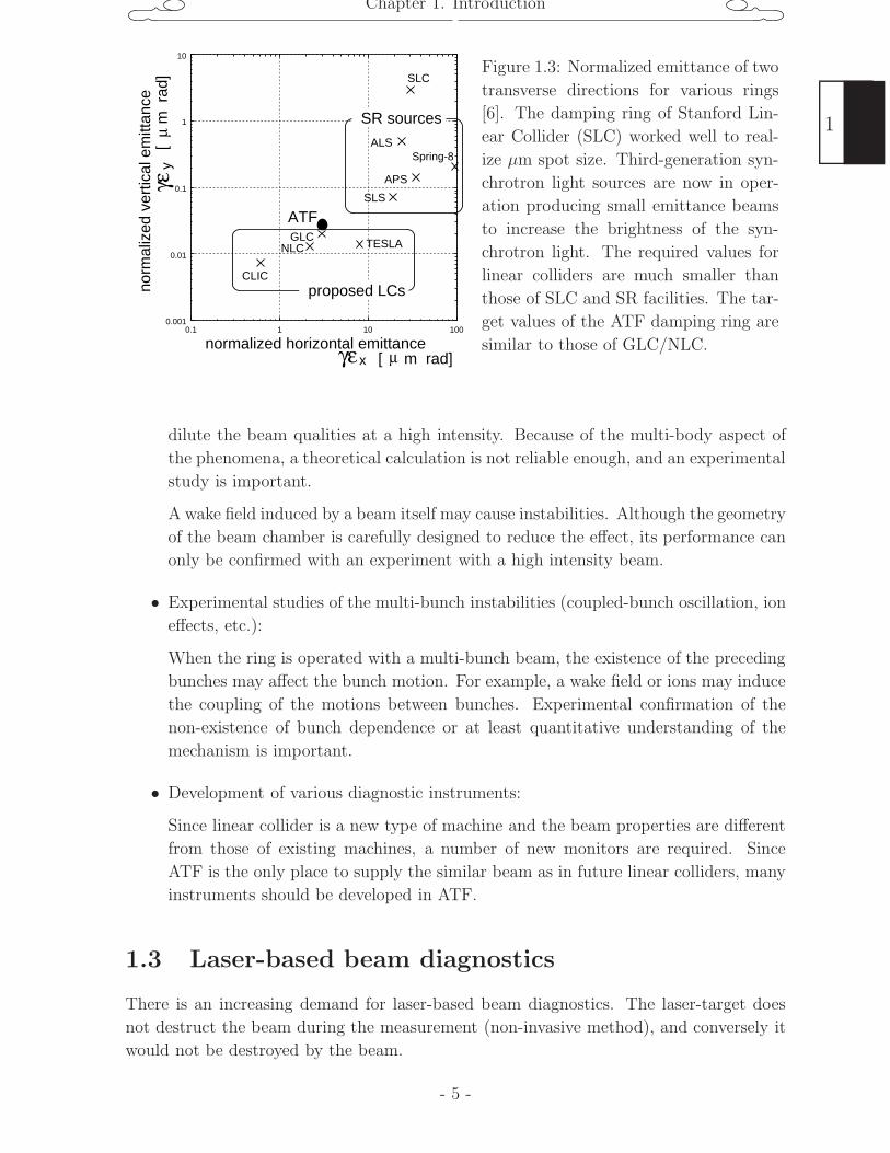
Figure 1.3 shows normalized emittances of two transverse directions for proposed lin-
ear colliders (at the exit of the damping ring) and for some existing accelerators and
storage rings. Here, the normalized emittance means γε, the product of the emittance
and particle’s γ-factor, and is a conserved quantity during acceleration. The emittance
required in future linear colliders has not yet been realized in any accelerators in the
world.
The Accelerator Test Facility (ATF) in KEK is an accelerator complex to study dy-
namics and techniques in generating a low-emittance beam required for linear colliders.
The damping ring is designed to produce a beam with similar qualities as required in
GLC/NLC. The items to be studied at the ATF damping ring are listed below:
• Establish techniques for precision magnet alignment and/or beam tuning method
to stably produce ultra-low-emittance beams:
Especially, the vertical emittance requires a severe magnet alignment tolerance and
a precise beam tuning. The most unambiguous way to prove this issue is to actually
produce and measure the beam with specified qualities.
• Experimental studies of the collective effects (intra-beam scattering, wake field,
etc.):
Due to the small emittance, electrons in a bunch are localized in a small volume.
A complex effect of many particles in a bunch, such as intra-beam scattering, may
1
- 4 -
Chapter 1. Introduction
0.001
0.01
0.1
1
10
0.1 1 10 100
SLC
SLS
ATF
NLCGLC
TESLA
CLIC
Spring-8
γε
γεy
x
[
m r
ad]
[ m rad]µ
µAPS
norm
aliz
ed v
ertic
al e
mitt
ance
normalized horizontal emittance
SR sources
proposed LCs
ALS
Figure 1.3: Normalized emittance of two
transverse directions for various rings
[6]. The damping ring of Stanford Lin-
ear Collider (SLC) worked well to real-
ize µm spot size. Third-generation syn-
chrotron light sources are now in oper-
ation producing small emittance beams
to increase the brightness of the syn-
chrotron light. The required values for
linear colliders are much smaller than
those of SLC and SR facilities. The tar-
get values of the ATF damping ring are
similar to those of GLC/NLC.
dilute the beam qualities at a high intensity. Because of the multi-body aspect of
the phenomena, a theoretical calculation is not reliable enough, and an experimental
study is important.
A wake field induced by a beam itself may cause instabilities. Although the geometry
of the beam chamber is carefully designed to reduce the effect, its performance can
only be confirmed with an experiment with a high intensity beam.
• Experimental studies of the multi-bunch instabilities (coupled-bunch oscillation, ion
effects, etc.):
When the ring is operated with a multi-bunch beam, the existence of the preceding
bunches may affect the bunch motion. For example, a wake field or ions may induce
the coupling of the motions between bunches. Experimental confirmation of the
non-existence of bunch dependence or at least quantitative understanding of the
mechanism is important.
• Development of various diagnostic instruments:
Since linear collider is a new type of machine and the beam properties are different
from those of existing machines, a number of new monitors are required. Since
ATF is the only place to supply the similar beam as in future linear colliders, many
instruments should be developed in ATF.
1.3 Laser-based beam diagnostics
There is an increasing demand for laser-based beam diagnostics. The laser-target does
not destruct the beam during the measurement (non-invasive method), and conversely it
would not be destroyed by the beam.
- 5 -
1
Chapter 1. Introduction
The most conventional device to measure the transverse beam profile is a wire scanner.
A solid wire of metal (tungsten or carbon) intersects the electron beam and the beam
profile is obtained by counting an appropriate background rate as a function of the relative
position of the wire and beam. This technique, however, cannot be used at any linear
colliders; the electron beam is so intense that solid wires would be quickly damaged. It
must be replaced by a laser-based technique.
In the linear colliders (and in their development work), laser-based beam profile mon-
itors will play an important role. These monitors utilize the Compton scattering process
of electrons with laser light. Many variations of the laser-based monitors have been de-
veloped. We mention two notable examples below.
The first is the so called laser-wire monitor. A focused laser beam is used as a wire to
scan the electron beam. The first laser-wire monitor was developed at SLAC to measure
the beam size at the interaction point of SLC (it was placed inside the detector) [7]. A
high power pulsed UV laser was focused by a refractive optics. It successfully measured 1
µm beam size with a laser beam focused down to ∼0.5 µm. A similar laser-wire system, to
be placed in the beam delivery system of future linear colliders, is proposed and is being
developed ([8]). A laserwire to measure the beam size in the damping ring was developed
in KEK-ATF. It played a crucial role in this work, and it will be detailed in Chapter 3.
The other example is the one which utilizes an interference pattern produced by two
laser beams. It was first successfully tested at SLAC in order to estimate a nano-meter
beam size at the FFTB [9]; the beam was scanned by the fine interference pattern.
In this thesis, studies of an ultra-low emittance electron beam in the damping ring
of KEK-ATF are presented. The beam emittances were measured by using the laserwire
beam profile monitor. An overview of the Accelerator Test Facility (ATF) is given in
Chapter 2. In Chapter 3, we describe the laserwire beam profile monitor, the most
important instrument for this work. Chapter 4 and 5 are the results of the experiment
done with a single-bunch and a multi-bunch beam, respectively. Chapter 6 is devoted to
the conclusion of this work.
A brief description of the beam dynamics in a storage ring is given in Appendix A.
In Appendix B, a new laserwire measurement method which enables to measure electron
beams smaller than laser width is described. We append the latest result of high intensity
multi-bunch measurement in Appendix C.
1
- 6 -
Chapter 2. The KEK Accelerator Test Facility
Chapter 2
The KEK Accelerator Test Facility
The KEK Accelerator Test Facility ( ATF ) [10] has been built as one of the steps toward
realization of future linear colliders; its main purpose is to establish production and ma-
nipulation techniques of a low emittance beam. In this chapter, we give a brief review of
the ATF itself, various monitors used for beam diagnostics, and beam tuning methods to
produce an extremely small emittance beam.
2.1 Overview of the accelerator complex
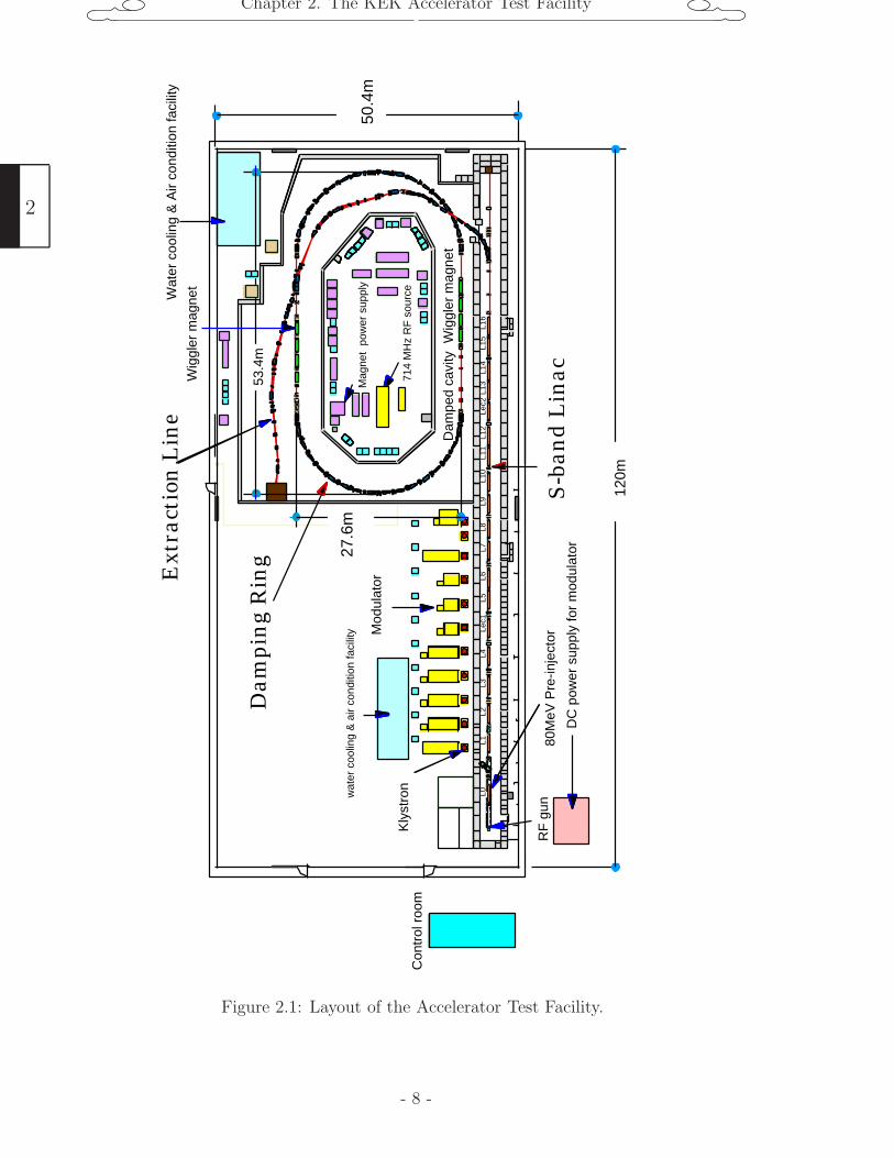
The layout of the facility is shown in Figure 2.1. It consists of three major parts: an
injector linac, a damping ring, and an extraction line. Below, we give a brief overview of
the beam line from upstream to downstream.
2.1.1 Electron-gun system
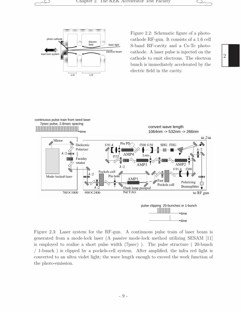
A photo-cathode RF-gun system has been used as a source of a low-emittance electron
beam 1. A schematic figure of the RF-gun is shown in Figure 2.2. A 1.6-cell S-band
RF cavity is excited in the π-mode resonance. A photo-cathode is made of a thin film
of Cs-Te alloy formed on the surface of a molybdenum plug. It is attached to the end
plate of the half-cell, where an electric field of about 100 MV/m is generated. A pulse of
ultra-violet laser light is injected on the photo-cathode to generate a bunch of electrons
via photo-electric emissions. A typical quantum efficiency of the cathode is 1%, and it
lasts more than one month in operation. An electron bunch is immediately accelerated by
the electric field in the cavity, and is further accelerated up to 80 MeV in a pre-injector.
The layout of the laser system is displayed in Figure 2.3. An infra red (λ=1064 nm)
mode-locked laser of 357 MHz (2.8 nsec spacing) is used as a seed laser beam. The required
laser pulse is structured ( single-bunch or 20-bunch ) in the first stage, and amplified in
a four-stage Nd:YAG amplifier pumped by flush-lamps. Then it is converted into ultra
violet (λ=266 nm) light and is transported to the RF-gun.
1Until 2001, the ATF had operated with a thermionic gun, a conventional electron-gun which utilizedthe thermionic emission of electrons. It was replaced by the RF-gun to improve the beam qualities atthe injector.
- 7 -
2
Chapter 2. The KEK Accelerator Test Facility
50.
4m
L1L2
L3L4
L5L6
L7L8
L9L1
0L1
1L1
2Le
c2L1
3L1
4L1
5L1
6Le
c1
120
m
Dam
ped
cavi
tyW
iggl
er m
agne
t
Wig
gler
mag
net
Wat
er c
oolin
g &
Air
cond
ition
faci
lity
Con
trol
roo
m
DC
pow
er s
uppl
y fo
r m
odul
ator
714
MH
z R
F s
ourc
e
53.
4m
27.
6m
80M
eV P
re-in
ject
or
L0
Mag
net
pow
er s
uppl
y
Dam
pin
g R
ingExt
ract
ion
Lin
e
S-b
and
Lin
acR
F g
un
wat
er c
oolin
g &
air
cond
ition
faci
lity M
odul
ator
Kly
stro
n
Figure 2.1: Layout of the Accelerator Test Facility.
2
- 8 -
Chapter 2. The KEK Accelerator Test Facility
Electricfield
electron beam
laser light
photo cathode
/2λ/4λ
load lock system
Figure 2.2: Schematic figure of a photo-
cathode RF-gun. It consists of a 1.6 cell
S-band RF-cavity and a Cs-Te photo-
cathode. A laser pulse is injected on the
cathode to emit electrons. The electron
bunch is immediately accelerated by the
electric field in the cavity.
continuous pulse train from seed laser7psec pulse, 2.8nsec spacing
pulse clipping 20-bunches or 1-bunch
time
time
time
convert wave length1064nm -> 532nm -> 266nm
Figure 2.3: Laser system for the RF-gun. A continuous pulse train of laser beam is
generated from a mode-lock laser (A passive mode-lock method utilizing SESAM [11]
is employed to realize a short pulse width (7psec) ). The pulse structure ( 20-bunch
/ 1-bunch ) is clipped by a pockels-cell system. After amplified, the infra red light is
converted to an ultra violet light; the wave length enough to exceed the work function of
the photo-emission.
- 9 -
2
Chapter 2. The KEK Accelerator Test Facility
2.1.2 Linac
The electron beam is accelerated to 1.28 GeV by an S-band (2856 MHz) linac, and is
injected into the damping ring. There are 8 units of RF system for regular acceleration,
and two special units for energy compensation.
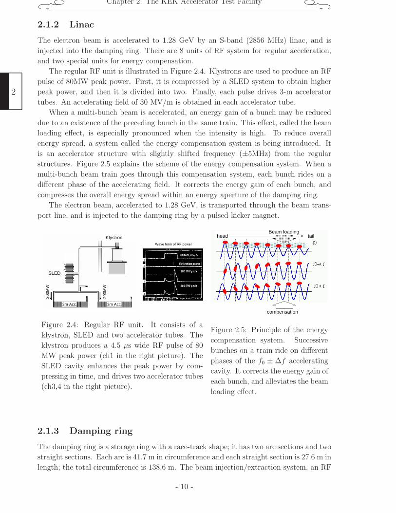
The regular RF unit is illustrated in Figure 2.4. Klystrons are used to produce an RF
pulse of 80MW peak power. First, it is compressed by a SLED system to obtain higher
peak power, and then it is divided into two. Finally, each pulse drives 3-m accelerator
tubes. An accelerating field of 30 MV/m is obtained in each accelerator tube.
When a multi-bunch beam is accelerated, an energy gain of a bunch may be reduced
due to an existence of the preceding bunch in the same train. This effect, called the beam
loading effect, is especially pronounced when the intensity is high. To reduce overall
energy spread, a system called the energy compensation system is being introduced. It
is an accelerator structure with slightly shifted frequency (±5MHz) from the regular
structures. Figure 2.5 explains the scheme of the energy compensation system. When a
multi-bunch beam train goes through this compensation system, each bunch rides on a
different phase of the accelerating field. It corrects the energy gain of each bunch, and
compresses the overall energy spread within an energy aperture of the damping ring.
The electron beam, accelerated to 1.28 GeV, is transported through the beam trans-
port line, and is injected to the damping ring by a pulsed kicker magnet.
1
2
3
4
Wave form of RF power
Klystron
SLED
200M
W
200M
W
3m Acc. 3m Acc.
Figure 2.4: Regular RF unit. It consists of a
klystron, SLED and two accelerator tubes. The
klystron produces a 4.5 µs wide RF pulse of 80
MW peak power (ch1 in the right picture). The
SLED cavity enhances the peak power by com-
pressing in time, and drives two accelerator tubes
(ch3,4 in the right picture).
compensation
head tailBeam loading
Figure 2.5: Principle of the energy
compensation system. Successive
bunches on a train ride on different
phases of the f0 ± ∆f accelerating
cavity. It corrects the energy gain of
each bunch, and alleviates the beam
loading effect.
2.1.3 Damping ring
The damping ring is a storage ring with a race-track shape; it has two arc sections and two
straight sections. Each arc is 41.7 m in circumference and each straight section is 27.6 m in
length; the total circumference is 138.6 m. The beam injection/extraction system, an RF
2
- 10 -
Chapter 2. The KEK Accelerator Test Facility
cavity and wiggler magnets are installed in the straight sections (the wigglers were being
turned off in this experiment). There are 96 beam position monitors (BPM) to measure
the beam orbit, and 48 horizontal and 50 vertical steering magnets for orbit correction.
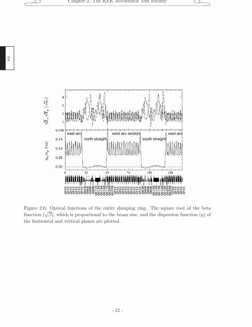
The optical functions, β and η, of the entire damping ring are plotted in Figure 2.6. The
vertical dispersion function ηy is zero around the entire ring, as stated in Sec. 1.2.
The role of the damping ring is to reduce emittance and momentum spread of the beam
through radiation damping process. The characteristic time of this damping process,
the damping time, is calculated to be about 20 msec without wiggler. Thus, the beam
reaches its equilibrium after injection in less than 200 msec. The horizontal emittance in
equilibrium condition is basically determined by the balance of radiation process (cooling)
and excitation process (heating), which in turn is determined by the lattice functions.
The best way to reduce the horizontal equilibrium emittance is to minimize the hor-
izontal dispersion at the bending part. A unique low-emittance lattice, called FOBO (a
periodic optics of a focusing quadrupole and a (combined-function) bending magnet), is
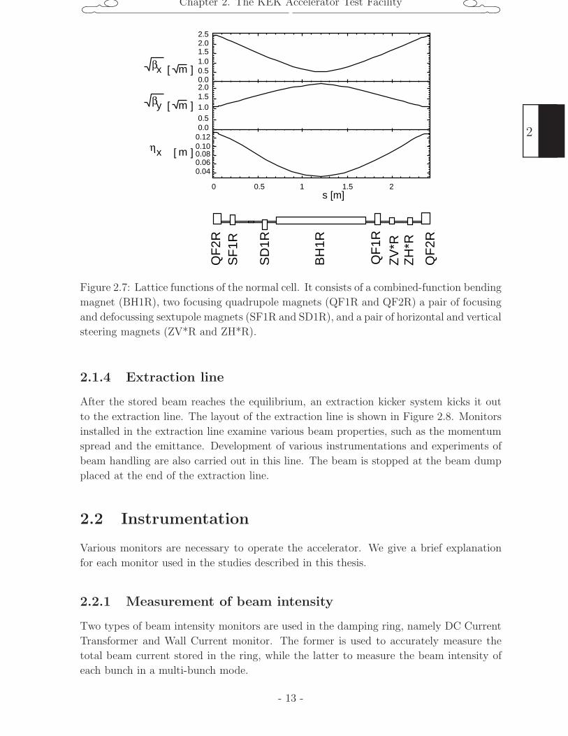
employed for this purpose. The lattice function of a FOBO cell is plotted in Figure 2.7. A
defocussing component of magnetic field is combined in the bending magnet. As a result,
the horizontal dispersion function is made small at the center of the bending magnet.
Each arc section is formed by 17 FOBO cells.
As for the vertical emittance, it is mostly originated from the imperfectness of the
machine. It can be reduced by precise alignment of the magnets and beam tuning. The
target value of the vertical emittance is less than 1% of the horizontal emittance.
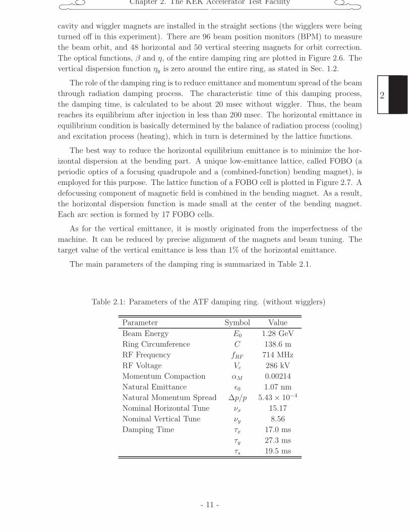
The main parameters of the damping ring is summarized in Table 2.1.
Table 2.1: Parameters of the ATF damping ring. (without wigglers)
Parameter Symbol Value
Beam Energy E0 1.28 GeV
Ring Circumference C 138.6 m
RF Frequency fRF 714 MHz
RF Voltage Vc 286 kV
Momentum Compaction αM 0.00214
Natural Emittance ε0 1.07 nm
Natural Momentum Spread ∆p/p 5.43 × 10⁻⁴
Nominal Horizontal Tune νx 15.17
Nominal Vertical Tune νy 8.56
Damping Time τx 17.0 ms
τy 27.3 ms
τs 19.5 ms
- 11 -
2
Chapter 2. The KEK Accelerator Test Facility
south straightnorth straightwest arc section east arc east arc
Figure 2.6: Optical functions of the entire damping ring. The square root of the beta
function (√β), which is proportional to the beam size, and the dispersion function (η) of
the horizontal and vertical planes are plotted.
2
- 12 -
Chapter 2. The KEK Accelerator Test Facility
0 0.5 1 1.5 2
0.040.060.080.100.120.00.51.01.52.00.00.51.01.52.02.5
s [m]
βx m[ ]
βy m[ ]
ηx m[ ]
QF
2R
QF
1R
SF
1R
SD
1R
BH
1R
ZV
*RZ
H*R
QF
2R
Figure 2.7: Lattice functions of the normal cell. It consists of a combined-function bending
magnet (BH1R), two focusing quadrupole magnets (QF1R and QF2R) a pair of focusing
and defocussing sextupole magnets (SF1R and SD1R), and a pair of horizontal and vertical
steering magnets (ZV*R and ZH*R).
2.1.4 Extraction line
After the stored beam reaches the equilibrium, an extraction kicker system kicks it out
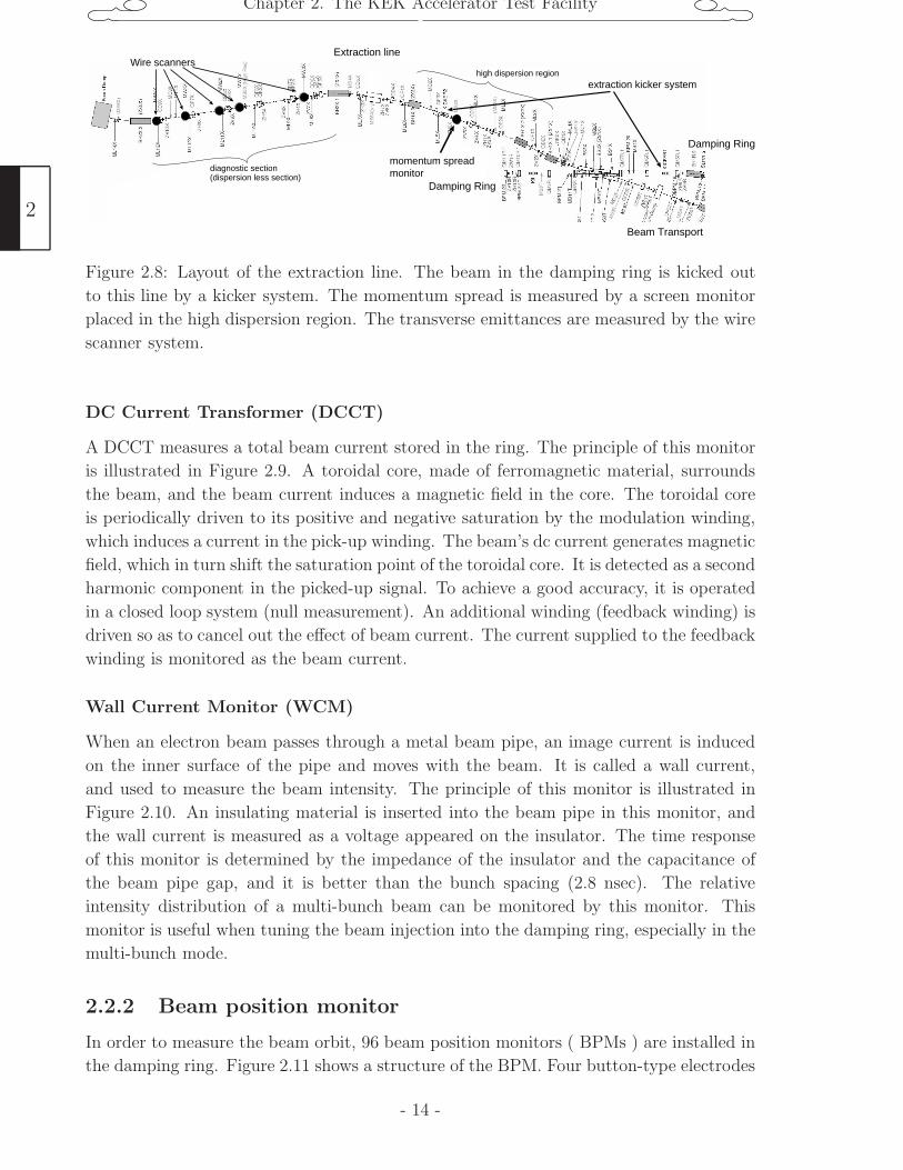
to the extraction line. The layout of the extraction line is shown in Figure 2.8. Monitors
installed in the extraction line examine various beam properties, such as the momentum
spread and the emittance. Development of various instrumentations and experiments of
beam handling are also carried out in this line. The beam is stopped at the beam dump
placed at the end of the extraction line.
2.2 Instrumentation
Various monitors are necessary to operate the accelerator. We give a brief explanation
for each monitor used in the studies described in this thesis.
2.2.1 Measurement of beam intensity
Two types of beam intensity monitors are used in the damping ring, namely DC Current
Transformer and Wall Current monitor. The former is used to accurately measure the
total beam current stored in the ring, while the latter to measure the beam intensity of
each bunch in a multi-bunch mode.
- 13 -
2
Chapter 2. The KEK Accelerator Test Facility
Extraction line
Damping Ring
Damping Ring
Beam Transport
diagnostic section(dispersion less section)
high dispersion regionWire scanners
momentum spreadmonitor
extraction kicker system
Figure 2.8: Layout of the extraction line. The beam in the damping ring is kicked out
to this line by a kicker system. The momentum spread is measured by a screen monitor
placed in the high dispersion region. The transverse emittances are measured by the wire
scanner system.
DC Current Transformer (DCCT)
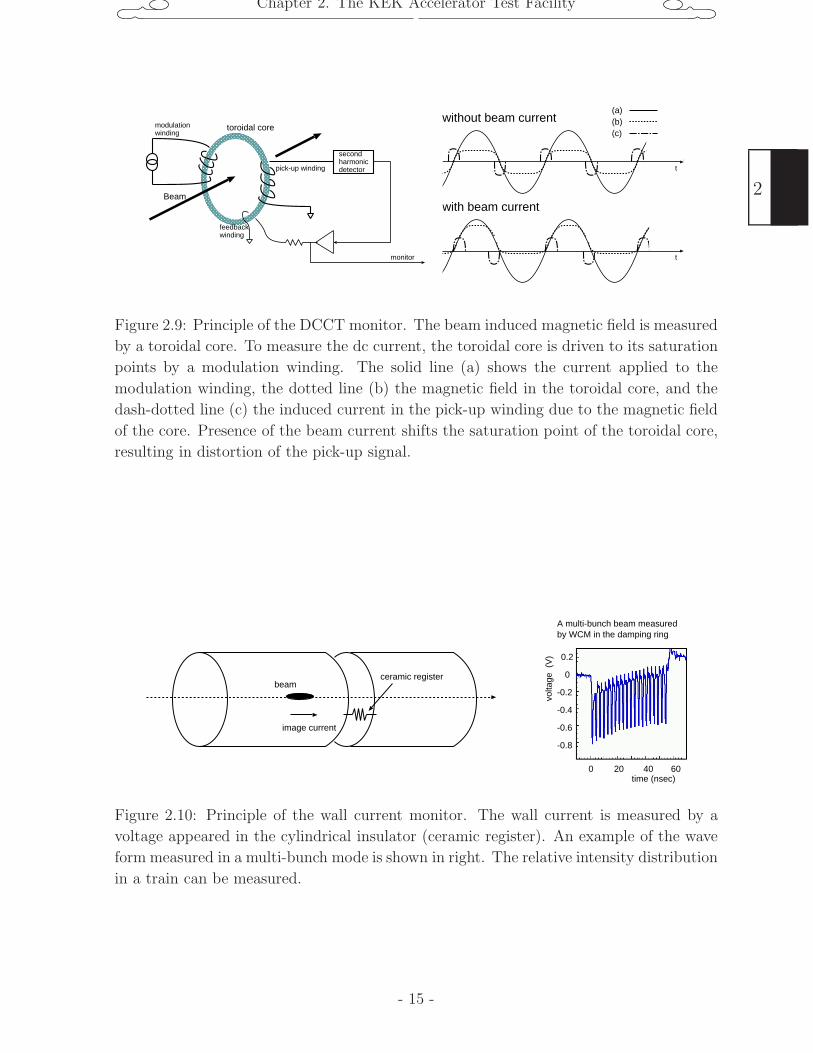
A DCCT measures a total beam current stored in the ring. The principle of this monitor
is illustrated in Figure 2.9. A toroidal core, made of ferromagnetic material, surrounds
the beam, and the beam current induces a magnetic field in the core. The toroidal core
is periodically driven to its positive and negative saturation by the modulation winding,
which induces a current in the pick-up winding. The beam’s dc current generates magnetic
field, which in turn shift the saturation point of the toroidal core. It is detected as a second
harmonic component in the picked-up signal. To achieve a good accuracy, it is operated
in a closed loop system (null measurement). An additional winding (feedback winding) is
driven so as to cancel out the effect of beam current. The current supplied to the feedback
winding is monitored as the beam current.
Wall Current Monitor (WCM)
When an electron beam passes through a metal beam pipe, an image current is induced
on the inner surface of the pipe and moves with the beam. It is called a wall current,
and used to measure the beam intensity. The principle of this monitor is illustrated in
Figure 2.10. An insulating material is inserted into the beam pipe in this monitor, and
the wall current is measured as a voltage appeared on the insulator. The time response
of this monitor is determined by the impedance of the insulator and the capacitance of
the beam pipe gap, and it is better than the bunch spacing (2.8 nsec). The relative
intensity distribution of a multi-bunch beam can be monitored by this monitor. This
monitor is useful when tuning the beam injection into the damping ring, especially in the
multi-bunch mode.
2.2.2 Beam position monitor
In order to measure the beam orbit, 96 beam position monitors ( BPMs ) are installed in
the damping ring. Figure 2.11 shows a structure of the BPM. Four button-type electrodes
2
- 14 -
Chapter 2. The KEK Accelerator Test Facility
Beam
toroidal core
pick-up winding
modulationwinding
secondharmonicdetector
feedbackwinding
without beam current
with beam current
t
monitor t
(a)(b)(c)
Figure 2.9: Principle of the DCCT monitor. The beam induced magnetic field is measured
by a toroidal core. To measure the dc current, the toroidal core is driven to its saturation
points by a modulation winding. The solid line (a) shows the current applied to the
modulation winding, the dotted line (b) the magnetic field in the toroidal core, and the
dash-dotted line (c) the induced current in the pick-up winding due to the magnetic field
of the core. Presence of the beam current shifts the saturation point of the toroidal core,
resulting in distortion of the pick-up signal.
ceramic registerbeam
image current
0
-0.2
-0.4
-0.6
-0.8
0.2
volta
ge (
V)
0 6020 40time (nsec)
A multi-bunch beam measured by WCM in the damping ring
Figure 2.10: Principle of the wall current monitor. The wall current is measured by a
voltage appeared in the cylindrical insulator (ceramic register). An example of the wave
form measured in a multi-bunch mode is shown in right. The relative intensity distribution
in a train can be measured.
- 15 -
2
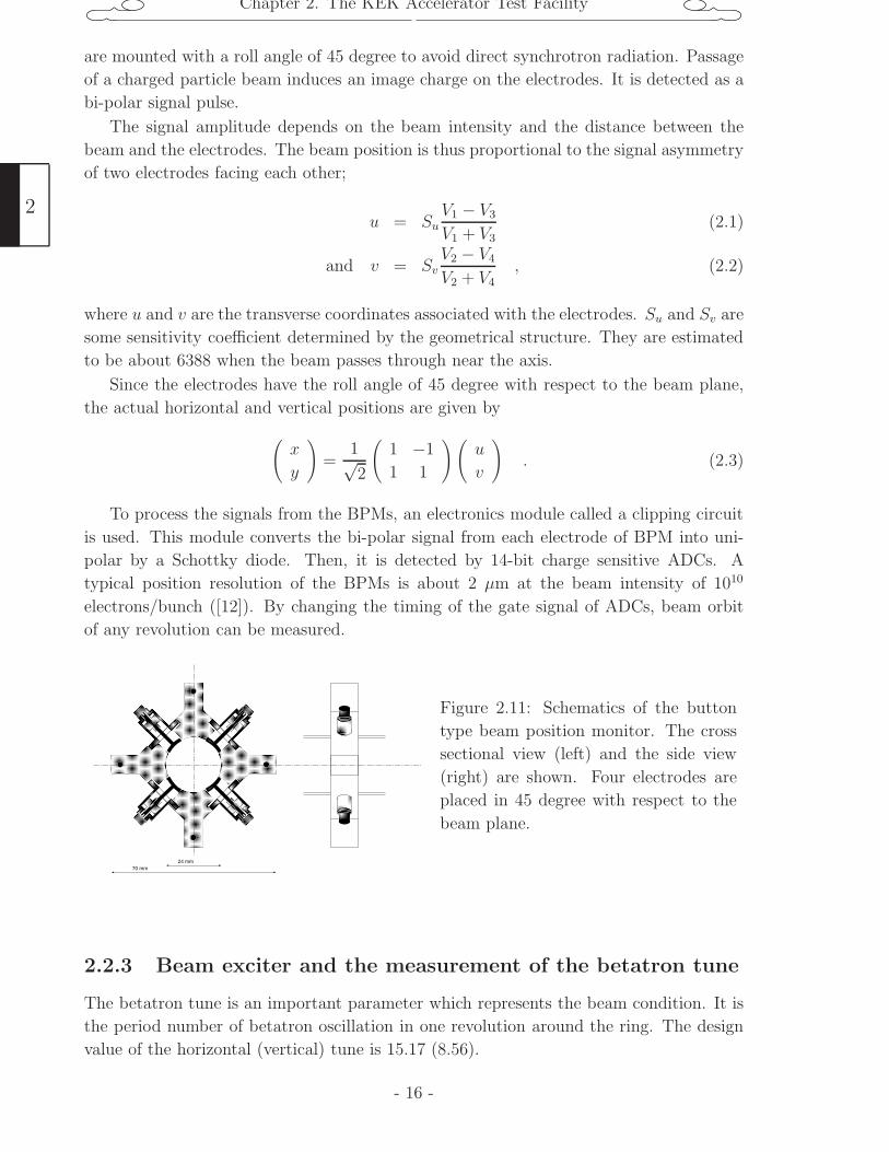
Chapter 2. The KEK Accelerator Test Facility
are mounted with a roll angle of 45 degree to avoid direct synchrotron radiation. Passage
of a charged particle beam induces an image charge on the electrodes. It is detected as a
bi-polar signal pulse.
The signal amplitude depends on the beam intensity and the distance between the
beam and the electrodes. The beam position is thus proportional to the signal asymmetry
of two electrodes facing each other;
u = SuV1 − V3
V1 + V3
(2.1)
and v = SvV2 − V4
V2 + V4
, (2.2)
where u and v are the transverse coordinates associated with the electrodes. Su and Sv are
some sensitivity coefficient determined by the geometrical structure. They are estimated
to be about 6388 when the beam passes through near the axis.
Since the electrodes have the roll angle of 45 degree with respect to the beam plane,
the actual horizontal and vertical positions are given by
(x
y
)=
1√2
(1 −1
1 1
)(u
v
). (2.3)
To process the signals from the BPMs, an electronics module called a clipping circuit
is used. This module converts the bi-polar signal from each electrode of BPM into uni-
polar by a Schottky diode. Then, it is detected by 14-bit charge sensitive ADCs. A
typical position resolution of the BPMs is about 2 µm at the beam intensity of 1010
electrons/bunch ([12]). By changing the timing of the gate signal of ADCs, beam orbit
of any revolution can be measured.
24 mm70 mm
Figure 2.11: Schematics of the button
type beam position monitor. The cross
sectional view (left) and the side view
(right) are shown. Four electrodes are
placed in 45 degree with respect to the
beam plane.
2.2.3 Beam exciter and the measurement of the betatron tune
The betatron tune is an important parameter which represents the beam condition. It is
the period number of betatron oscillation in one revolution around the ring. The design
value of the horizontal (vertical) tune is 15.17 (8.56).
2
- 16 -
Chapter 2. The KEK Accelerator Test Facility
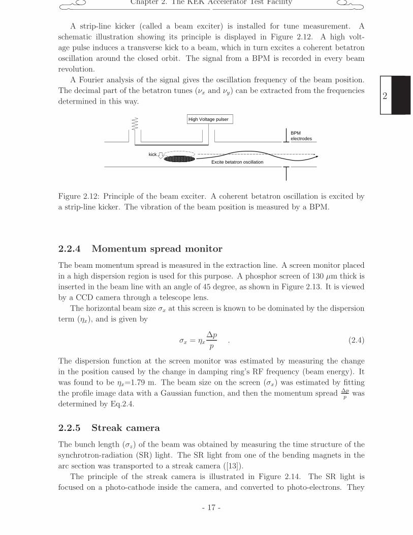
A strip-line kicker (called a beam exciter) is installed for tune measurement. A
schematic illustration showing its principle is displayed in Figure 2.12. A high volt-
age pulse induces a transverse kick to a beam, which in turn excites a coherent betatron
oscillation around the closed orbit. The signal from a BPM is recorded in every beam
revolution.
A Fourier analysis of the signal gives the oscillation frequency of the beam position.
The decimal part of the betatron tunes (νx and νy) can be extracted from the frequencies
determined in this way.
High Voltage pulser
Excite betatron oscillation
kick
BPMelectrodes
Figure 2.12: Principle of the beam exciter. A coherent betatron oscillation is excited by
a strip-line kicker. The vibration of the beam position is measured by a BPM.
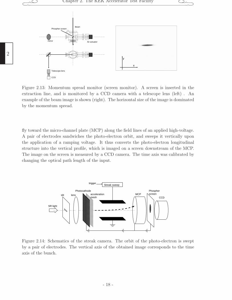
2.2.4 Momentum spread monitor
The beam momentum spread is measured in the extraction line. A screen monitor placed
in a high dispersion region is used for this purpose. A phosphor screen of 130 µm thick is
inserted in the beam line with an angle of 45 degree, as shown in Figure 2.13. It is viewed
by a CCD camera through a telescope lens.
The horizontal beam size σx at this screen is known to be dominated by the dispersion
term (ηx), and is given by
σx = ηx∆p
p. (2.4)
The dispersion function at the screen monitor was estimated by measuring the change
in the position caused by the change in damping ring’s RF frequency (beam energy). It
was found to be ηx=1.79 m. The beam size on the screen (σx) was estimated by fitting
the profile image data with a Gaussian function, and then the momentum spread ∆pp
was
determined by Eq.2.4.
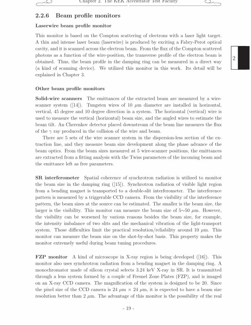
2.2.5 Streak camera
The bunch length (σz) of the beam was obtained by measuring the time structure of the
synchrotron-radiation (SR) light. The SR light from one of the bending magnets in the
arc section was transported to a streak camera ([13]).
The principle of the streak camera is illustrated in Figure 2.14. The SR light is
focused on a photo-cathode inside the camera, and converted to photo-electrons. They
- 17 -
2
Chapter 2. The KEK Accelerator Test Facility
Beam
CCD
Telescope lens
Air actuator
Phospher screen
mirror
x
y
Figure 2.13: Momentum spread monitor (screen monitor). A screen is inserted in the
extraction line, and is monitored by a CCD camera with a telescope lens (left) . An
example of the beam image is shown (right). The horizontal size of the image is dominated
by the momentum spread.
fly toward the micro-channel plate (MCP) along the field lines of an applied high-voltage.
A pair of electrodes sandwiches the photo-electron orbit, and sweeps it vertically upon
the application of a ramping voltage. It thus converts the photo-electron longitudinal
structure into the vertical profile, which is imaged on a screen downstream of the MCP.
The image on the screen is measured by a CCD camera. The time axis was calibrated by
changing the optical path length of the input.
MCPPhospherscreen
CCD
Photocathode
lensslit accelerationmesh
Streak sweeptrigger
SR light
Figure 2.14: Schematics of the streak camera. The orbit of the photo-electron is swept
by a pair of electrodes. The vertical axis of the obtained image corresponds to the time
axis of the bunch.
2
- 18 -
Chapter 2. The KEK Accelerator Test Facility
2.2.6 Beam profile monitors
Laserwire beam profile monitor
This monitor is based on the Compton scattering of electrons with a laser light target.
A thin and intense laser beam (laserwire) is produced by exciting a Fabry-Perot optical
cavity, and it is scanned across the electron beam. From the flux of the Compton scattered
photons as a function of the wire-position, the transverse profile of the electron beam is
obtained. Thus, the beam profile in the damping ring can be measured in a direct way
(a kind of scanning device). We utilized this monitor in this work. Its detail will be
explained in Chapter 3.
Other beam profile monitors
Solid-wire scanners The emittances of the extracted beam are measured by a wire-
scanner system ([14]). Tungsten wires of 10 µm diameter are installed in horizontal,
vertical, 45 degree and 10 degree direction in a system. The horizontal (vertical) wire is
used to measure the vertical (horizontal) beam size, and the angled wires to estimate the
beam tilt. An Cherenkov detector placed downstream of the beam line measures the flux
of the γ ray produced in the collision of the wire and beam.
There are 5 sets of the wire scanner system in the dispersion-less section of the ex-
traction line, and they measure beam size development along the phase advance of the
beam optics. From the beam sizes measured at 5 wire-scanner positions, the emittances
are extracted from a fitting analysis with the Twiss parameters of the incoming beam and
the emittance left as free parameters.
SR interferometer Spatial coherence of synchrotron radiation is utilized to monitor
the beam size in the damping ring ([15]). Synchrotron radiation of visible light region
from a bending magnet is transported to a double-slit interferometer. The interference
pattern is measured by a triggerable CCD camera. From the visibility of the interference
pattern, the beam sizes at the source can be estimated. The smaller is the beam size, the
larger is the visibility. This monitor can measure the beam size of 5∼50 µm. However,
the visibility can be worsened by various reasons besides the beam size, for example,
the intensity imbalance of two slits and the mechanical vibration of the light-transport
system. Those difficulties limit the practical resolution/reliability around 10 µm. This
monitor can measure the beam size on the shot-by-shot basis. This property makes the
monitor extremely useful during beam tuning procedures.
FZP monitor A kind of microscope in X-ray region is being developed ([16]). This
monitor also uses synchrotron radiation from a bending magnet in the damping ring. A
monochromator made of silicon crystal selects 3.24 keV X-ray in SR. It is transmitted
through a lens system formed by a couple of Fresnel Zone Plates (FZP), and is imaged
on an X-ray CCD camera. The magnification of the system is designed to be 20. Since
the pixel size of the CCD camera is 24 µm × 24 µm, it is expected to have a beam size
resolution better than 2 µm. The advantage of this monitor is the possibility of the real
- 19 -
2
Chapter 2. The KEK Accelerator Test Facility
time measurement of two-dimensional beam profiles. It requires only 20 msec of exposure
time to obtain enough signals. Not only the beam sizes but also the tilt of the profile can
be measured. The system is still under development. The systematic effects caused by
misalignments of the FZP lenses are being studied.
ODR monitor A beam size monitor based on the optical diffraction radiation (ODR)
is being developed in the extraction line ([17]) . ODR is a kind of wake-fields generated
by a passage of an electron beam near a conductive object. Actually, a metal slit with an
aperture of 260 µm is placed in the beam line. When an electron beam passes through
the slit, radiations of visible light are emitted from both edges of the slit. They generate
an interference pattern, which contains information of the beam size. Its sensitivity to
the beam size depends upon the slit width. An image-intensifier tube (IIT) and a CCD
camera placed 3 m from the slit detect the profile of the radiations. In principle, this
monitor can measure the beam size in a single passage of a beam, making of an extremely
fast monitor free from the jitter of beam orbit. The difficulty is the fabrication of the metal
slit. Flatness over a large area and sharpness of the slit edges are crucial. The SR light
from a bending magnet can be backgrounds to the detected light. Further development
works are required to make a reliable beam size monitor.
2.3 Production of a low emittance beam
As explained in Sec. 1.2 and Sec. 2.1.3, the horizontal emittance is basically determined by
the ring’s optics functions. This ideal emittance is sometime called a natural emittance,
and is expected to be realized actually when the current intensity is low (no collective
effects). As for the vertical emittance, its ideal value is extremely small, and the actual
emittance is determined by various errors (imperfection) of the ring’s optics functions
caused by misalignments and field errors of the magnets.
In this section, we describe various efforts needed to minimize the errors in the optics
function, and explain how to achieve a ultra-low vertical emittance.
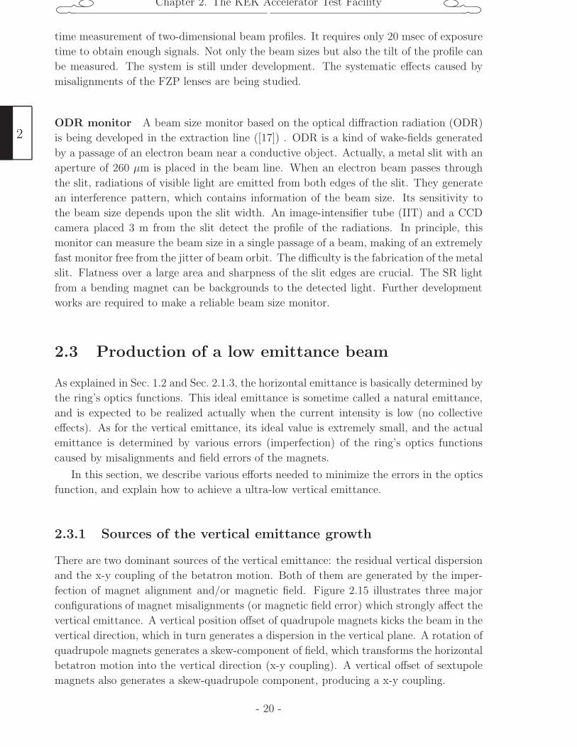
2.3.1 Sources of the vertical emittance growth
There are two dominant sources of the vertical emittance: the residual vertical dispersion
and the x-y coupling of the betatron motion. Both of them are generated by the imper-
fection of magnet alignment and/or magnetic field. Figure 2.15 illustrates three major
configurations of magnet misalignments (or magnetic field error) which strongly affect the
vertical emittance. A vertical position offset of quadrupole magnets kicks the beam in the
vertical direction, which in turn generates a dispersion in the vertical plane. A rotation of
quadrupole magnets generates a skew-component of field, which transforms the horizontal
betatron motion into the vertical direction (x-y coupling). A vertical offset of sextupole
magnets also generates a skew-quadrupole component, producing a x-y coupling.
2
- 20 -
Chapter 2. The KEK Accelerator Test Facility
N
NS
S N
NS
SS
N
S
N
S
N
(a) Quadrupole offset (b) Quadrupole rotation (c) Sextupole offset
Figure 2.15: Various misalignments of the magnets. The cross point of the dot-dashed
lines indicates the central beam orbit.
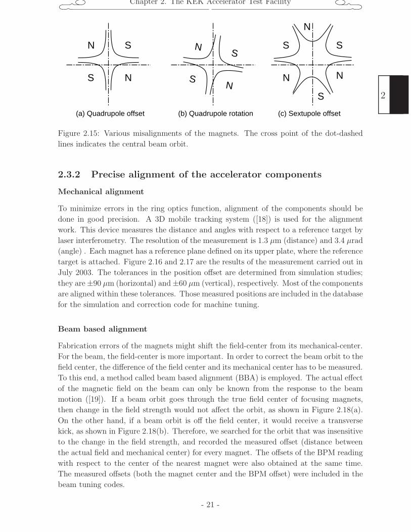
2.3.2 Precise alignment of the accelerator components
Mechanical alignment
To minimize errors in the ring optics function, alignment of the components should be
done in good precision. A 3D mobile tracking system ([18]) is used for the alignment
work. This device measures the distance and angles with respect to a reference target by
laser interferometry. The resolution of the measurement is 1.3 µm (distance) and 3.4 µrad
(angle) . Each magnet has a reference plane defined on its upper plate, where the reference
target is attached. Figure 2.16 and 2.17 are the results of the measurement carried out in
July 2003. The tolerances in the position offset are determined from simulation studies;
they are ±90 µm (horizontal) and ±60 µm (vertical), respectively. Most of the components
are aligned within these tolerances. Those measured positions are included in the database
for the simulation and correction code for machine tuning.
Beam based alignment
Fabrication errors of the magnets might shift the field-center from its mechanical-center.
For the beam, the field-center is more important. In order to correct the beam orbit to the
field center, the difference of the field center and its mechanical center has to be measured.
To this end, a method called beam based alignment (BBA) is employed. The actual effect
of the magnetic field on the beam can only be known from the response to the beam
motion ([19]). If a beam orbit goes through the true field center of focusing magnets,
then change in the field strength would not affect the orbit, as shown in Figure 2.18(a).
On the other hand, if a beam orbit is off the field center, it would receive a transverse
kick, as shown in Figure 2.18(b). Therefore, we searched for the orbit that was insensitive
to the change in the field strength, and recorded the measured offset (distance between
the actual field and mechanical center) for every magnet. The offsets of the BPM reading
with respect to the center of the nearest magnet were also obtained at the same time.
The measured offsets (both the magnet center and the BPM offset) were included in the
beam tuning codes.
- 21 -
2
Chapter 2. The KEK Accelerator Test Facility
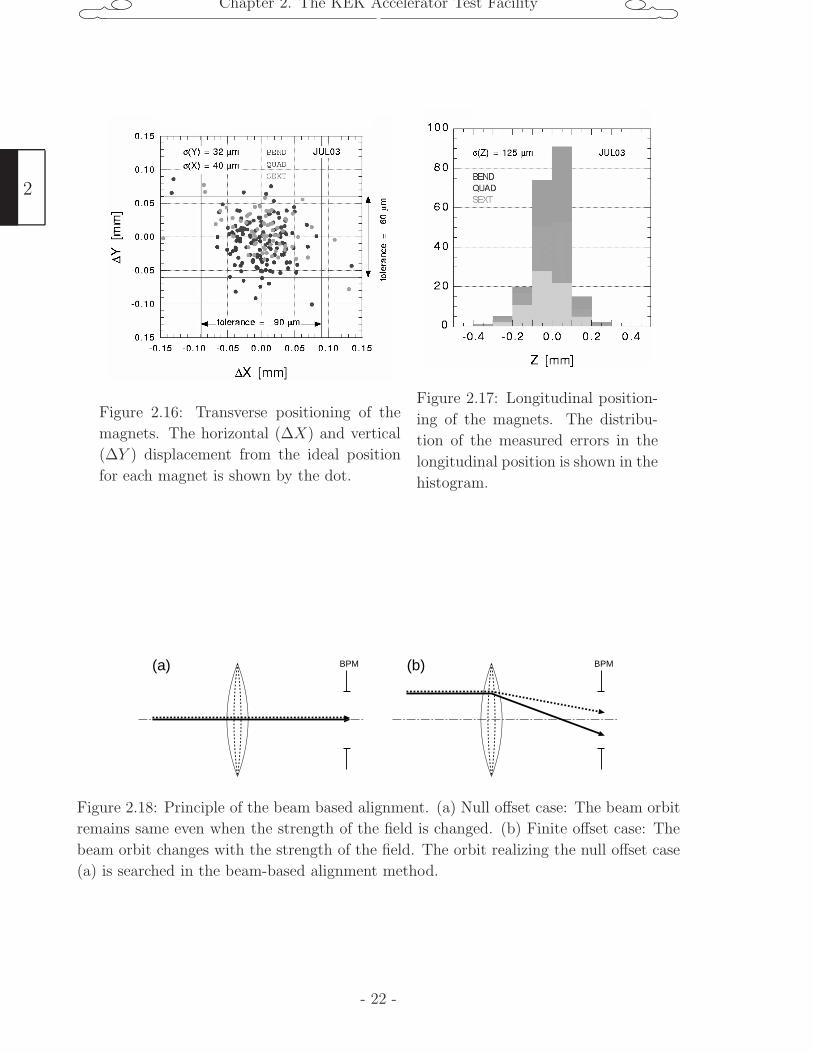
Figure 2.16: Transverse positioning of the
magnets. The horizontal (∆X) and vertical
(∆Y ) displacement from the ideal position
for each magnet is shown by the dot.
Figure 2.17: Longitudinal position-
ing of the magnets. The distribu-
tion of the measured errors in the
longitudinal position is shown in the
histogram.
(b)(a) BPMBPM
Figure 2.18: Principle of the beam based alignment. (a) Null offset case: The beam orbit
remains same even when the strength of the field is changed. (b) Finite offset case: The
beam orbit changes with the strength of the field. The orbit realizing the null offset case
(a) is searched in the beam-based alignment method.
2
- 22 -
Chapter 2. The KEK Accelerator Test Facility
2.3.3 Beam tuning
The final tuning to minimize the vertical emittance is done by a combined correction
of COD-dispersion using the steering magnets, and by x-y coupling correction using the
skew magnets. All those methods are based only on the measurement of beam orbit ([20])
and trial and error procedures with beam size monitoring is not necessary.
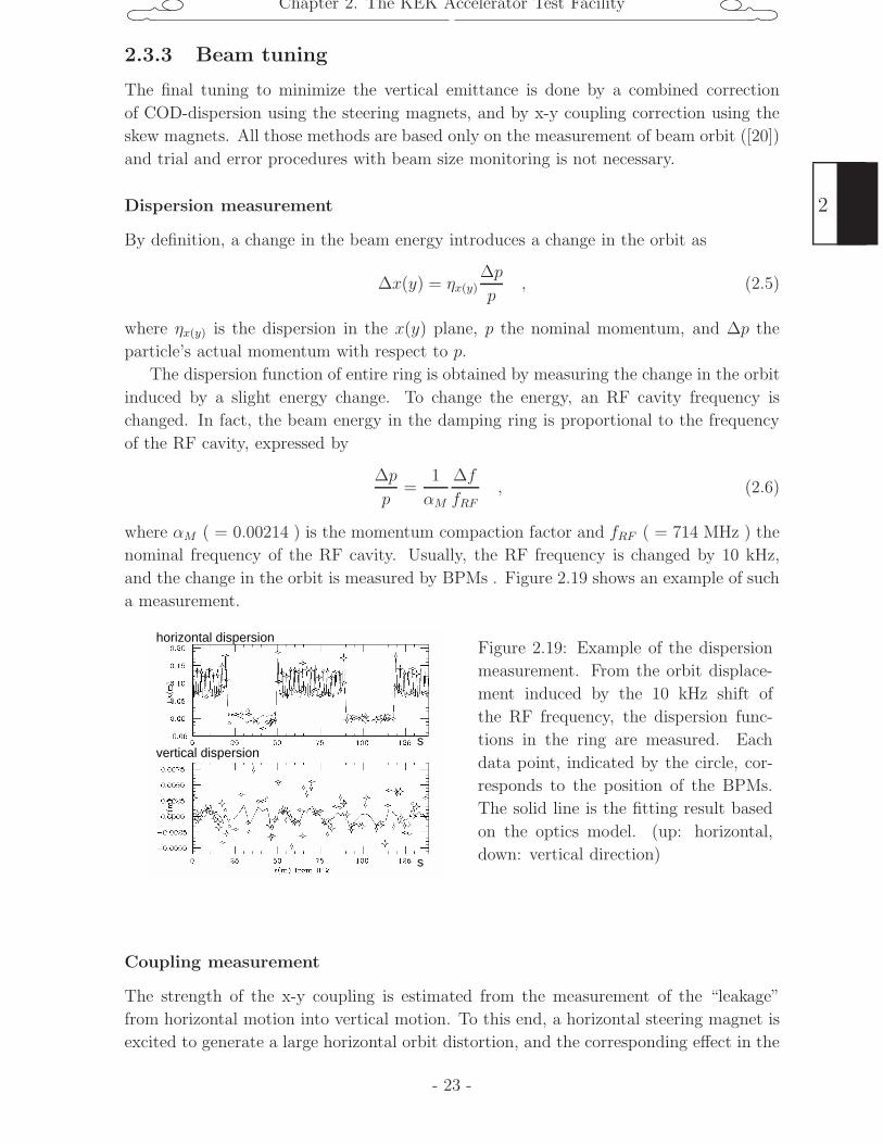
Dispersion measurement
By definition, a change in the beam energy introduces a change in the orbit as
∆x(y) = ηx(y)∆p
p, (2.5)
where ηx(y) is the dispersion in the x(y) plane, p the nominal momentum, and ∆p the
particle’s actual momentum with respect to p.
The dispersion function of entire ring is obtained by measuring the change in the orbit
induced by a slight energy change. To change the energy, an RF cavity frequency is
changed. In fact, the beam energy in the damping ring is proportional to the frequency
of the RF cavity, expressed by
∆p
p=
1
αM
∆f
fRF, (2.6)
where αM ( = 0.00214 ) is the momentum compaction factor and fRF ( = 714 MHz ) the
nominal frequency of the RF cavity. Usually, the RF frequency is changed by 10 kHz,
and the change in the orbit is measured by BPMs . Figure 2.19 shows an example of such
a measurement.
horizontal dispersion
vertical dispersions
s
Figure 2.19: Example of the dispersion
measurement. From the orbit displace-
ment induced by the 10 kHz shift of
the RF frequency, the dispersion func-
tions in the ring are measured. Each
data point, indicated by the circle, cor-
responds to the position of the BPMs.
The solid line is the fitting result based
on the optics model. (up: horizontal,
down: vertical direction)
Coupling measurement
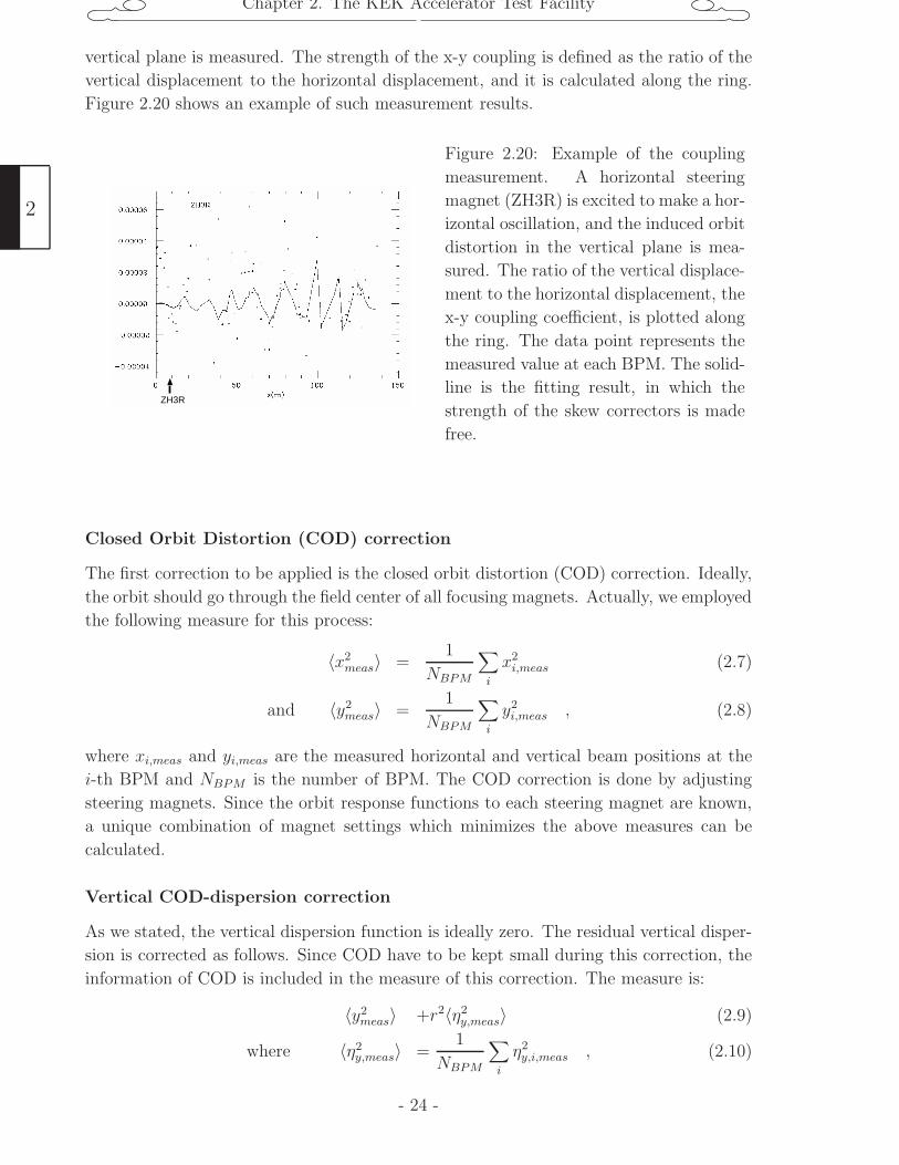
The strength of the x-y coupling is estimated from the measurement of the “leakage”
from horizontal motion into vertical motion. To this end, a horizontal steering magnet is
excited to generate a large horizontal orbit distortion, and the corresponding effect in the
- 23 -
2
Chapter 2. The KEK Accelerator Test Facility
vertical plane is measured. The strength of the x-y coupling is defined as the ratio of the
vertical displacement to the horizontal displacement, and it is calculated along the ring.
Figure 2.20 shows an example of such measurement results.
ZH3R
Figure 2.20: Example of the coupling
measurement. A horizontal steering
magnet (ZH3R) is excited to make a hor-
izontal oscillation, and the induced orbit
distortion in the vertical plane is mea-
sured. The ratio of the vertical displace-
ment to the horizontal displacement, the
x-y coupling coefficient, is plotted along
the ring. The data point represents the
measured value at each BPM. The solid-
line is the fitting result, in which the
strength of the skew correctors is made
free.
Closed Orbit Distortion (COD) correction
The first correction to be applied is the closed orbit distortion (COD) correction. Ideally,
the orbit should go through the field center of all focusing magnets. Actually, we employed
the following measure for this process:
〈x2meas〉 =
1
NBPM
∑i
x2i,meas (2.7)
and 〈y2meas〉 =
1
NBPM
∑i
y2i,meas , (2.8)
where xi,meas and yi,meas are the measured horizontal and vertical beam positions at the
i-th BPM and NBPM is the number of BPM. The COD correction is done by adjusting
steering magnets. Since the orbit response functions to each steering magnet are known,
a unique combination of magnet settings which minimizes the above measures can be
calculated.
Vertical COD-dispersion correction
As we stated, the vertical dispersion function is ideally zero. The residual vertical disper-
sion is corrected as follows. Since COD have to be kept small during this correction, the
information of COD is included in the measure of this correction. The measure is:
〈y2meas〉 +r2〈η2
y,meas〉 (2.9)
where 〈η2y,meas〉 =
1
NBPM
∑i
η2y,i,meas , (2.10)
2
- 24 -
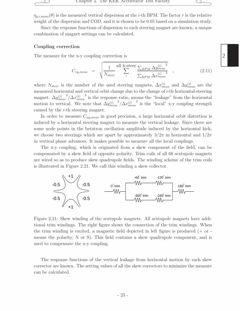
Chapter 2. The KEK Accelerator Test Facility
ηy,i,meas(θ) is the measured vertical dispersion at the i-th BPM. The factor r is the relative
weight of the dispersion and COD, and it is chosen to be 0.05 based on a simulation study.
Since the response functions of dispersion to each steering magnet are known, a unique
combination of magnet settings can be calculated.
Coupling correction
The measure for the x-y coupling correction is
Cxy,meas =
√√√√√ 1
Nsteer
all h-steer∑i
∑BPM ∆y
(i)meas
2
∑BPM ∆x
(i)meas
2 , (2.11)
where Nsteer is the number of the used steering magnets, ∆x(i)meas and ∆y(i)
meas are the
measured horizontal and vertical orbit change due to the change of i-th horizontal-steering
magnet. ∆y(i)meas
2/∆x(i)
meas
2is the response ratio, means the “leakage” from the horizontal
motion to vertical. We note that ∆y(i)meas
2/∆x(i)
meas
2is the “local” x-y coupling strength
caused by the i-th steering magnet.
In order to measure Cxy,meas in good precision, a large horizontal orbit distortion is
induced by a horizontal steering magnet to measure the vertical leakage. Since there are
some node points in the betatron oscillation amplitude induced by the horizontal kick,
we choose two steerings which are apart by approximately 3/2π in horizontal and 1/2π
in vertical phase advances. It makes possible to measure all the local couplings.
The x-y coupling, which is originated from a skew component of the field, can be
compensated by a skew field of opposite polarity. Trim coils of all 68 sextupole magnets
are wired so as to produce skew quadrupole fields. The winding scheme of the trim coils
is illustrated in Figure 2.21. We call this winding a skew collector.
-0.5
-0.5
-0.5
-0.5
+1
+1
0 trim
-60 trim -120 trim
-300 trim -240 trim
180 trim
Figure 2.21: Skew winding of the sextupole magnets. All sextupole magnets have addi-
tional trim windings. The right figure shows the connection of the trim windings. When
the trim winding is excited, a magnetic field depicted in left figure is produced (+ or -
means the polarity, N or S). This field contains a skew quadrupole component, and is
used to compensate the x-y coupling.
The response functions of the vertical leakage from horizontal motion by each skew
corrector are known. The setting values of all the skew correctors to minimize the measure
can be calculated.
- 25 -
2
Chapter 2. The KEK Accelerator Test Facility
Expected vertical emittance
The usefulness of the beam tuning procedure described above was confirmed by a com-
puter simulation code called SAD. In the simulation, the mechanical misalignment of
the magnets and the offset of the BPM are taken into account as actually measured. In
addition, to allow residual magnet errors, alignment offset and rotation errors are ran-
domly added. These errors are generated according to a Gaussian distribution with their
rms width given in Table 2.2. Then the SAD simulation program calculates the vertical
emittance for a given magnet setting. A series of correction procedures (COD ⇒ COD-
dispersion ⇒ coupling correction) is made in the same manner as the actual beam tuning.
The final value for the vertical emittance after the entire process depends upon the initial
magnet setting given in the simulation. To understand and estimate the impact of initial
conditions, the simulation is repeated 500 times with different initial conditions chosen
randomly. The distribution of the resultant vertical emittance are plotted in Figure 2.22
at the each stage of the correction processes. We can conclude from the figure that each
correction procedure is effective in reducing the vertical emittance, and that the target
value (1 × 10⁻¹¹ rad·m) can be achieved with a strong possibility. At the same time, the
alignment tolerance for magnets and the requirement of the BPM resolution are deter-
mined. The experimental confirmation of the low emittance achievement will be explained
in Chapter 4.
Table 2.2: Random errors applied to the magnets in the simulation.
components applied random errors (rms)
Offset of magnets 30 µm
Rotation of magnets 300 µrad
Offset of BPM 300 µm
Rotation of BPM 20 mrad
2
- 26 -
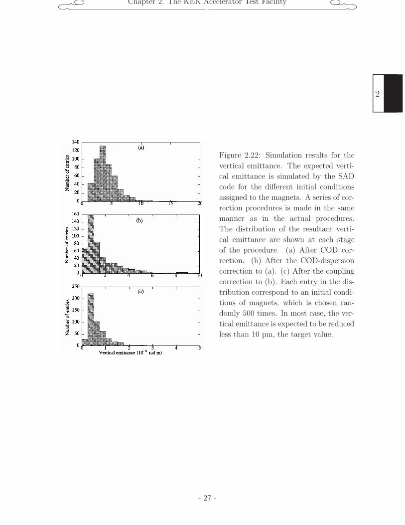
Chapter 2. The KEK Accelerator Test Facility
Figure 2.22: Simulation results for the
vertical emittance. The expected verti-
cal emittance is simulated by the SAD
code for the different initial conditions
assigned to the magnets. A series of cor-
rection procedures is made in the same
manner as in the actual procedures.
The distribution of the resultant verti-
cal emittance are shown at each stage
of the procedure. (a) After COD cor-
rection. (b) After the COD-dispersion
correction to (a). (c) After the coupling
correction to (b). Each entry in the dis-
tribution correspond to an initial condi-
tions of magnets, which is chosen ran-
domly 500 times. In most case, the ver-
tical emittance is expected to be reduced
less than 10 pm, the target value.
- 27 -
2
Chapter 3. Laserwire Beam Profile Monitor
Chapter 3
Laserwire Beam Profile Monitor
In this chapter, we describe the laserwire beam profile monitor, the most important
instrument for this work. This monitor directly measures the transverse profiles (in both
vertical and horizontal directions) of the electron beam in the damping ring. All emittance
measurements described in this thesis were done with this monitor. The development
works of this monitor have been detailed in [22], [23] and [24].
3.1 Principle of the laserwire monitor
3.1.1 Principle of the measurement
The principle of the beam profile measurement using this monitor is as follows. Install a
very thin laser beam (laserwire) in an electron beam orbit perpendicularly to the beam
line as shown in Figure 3.1. When an electron beam crosses the laserwire, some of the
electrons interact with the laser lights, and emit energetic photons in the forward direction
via the Compton scattering process. A detector placed downstream of the collision point
measures the flux of the scattered photons. By scanning a position of the laserwire
across the electron beam while measuring the signal count rate; a transverse profile of
the electron beam is obtained. Suppose both electron and laser beams have a Gaussian
intensity distribution ( with rms width σe and σlw, respectively ), the measured profile is
also a Gaussian shape with rms width σmeas (expressed by σ2meas = σ2
e + σ2lw). The actual
size of the electron beam can be calculated by subtracting the width of the laserwire from
the measured profile.
The important requirements for this monitor are as follows: make a laser beam thin
enough to measure the width of a small electron beam, and to realize a laser intensity as
high as possible to identify a signal among backgrounds of the beam line.
3.1.2 Compton scattering
First of all, we consider the differential cross section of the Compton scattering process
and estimate the counting rate of the signal photon. In our case, a high energy electron
hits a photon of visible wavelength and emits a high energy photon. (This process is
sometimes called the inverse-Compton scattering.) We first calculate this process in the
3
- 28 -
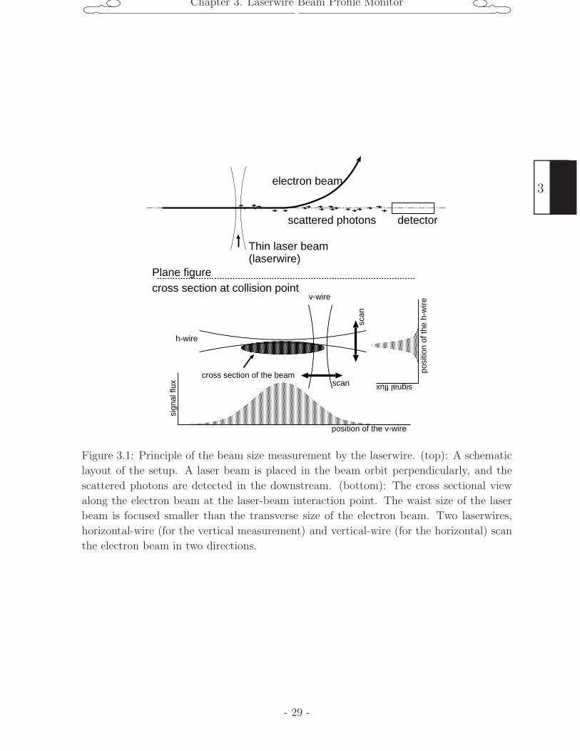
Chapter 3. Laserwire Beam Profile Monitor
sign
al fl
ux signal flux
position of the v-wirepo
sitio
n of
the
h-w
ire
scan
scan
h-wire
v-wire
cross section of the beam
detector
electron beam
Thin laser beam (laserwire)
scattered photons
Plane figurecross section at collision point
Figure 3.1: Principle of the beam size measurement by the laserwire. (top): A schematic
layout of the setup. A laser beam is placed in the beam orbit perpendicularly, and the
scattered photons are detected in the downstream. (bottom): The cross sectional view
along the electron beam at the laser-beam interaction point. The waist size of the laser
beam is focused smaller than the transverse size of the electron beam. Two laserwires,
horizontal-wire (for the vertical measurement) and vertical-wire (for the horizontal) scan
the electron beam in two directions.
- 29 -
3
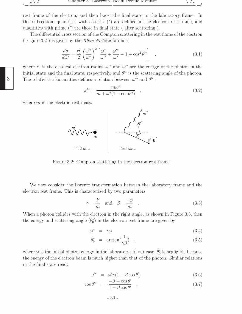
Chapter 3. Laserwire Beam Profile Monitor
rest frame of the electron, and then boost the final state to the laboratory frame. In
this subsection, quantities with asterisk (∗) are defined in the electron rest frame, and
quantities with prime (′) are those in final state ( after scattering ).
The differential cross section of the Compton scattering in the rest flame of the electron
( Figure 3.2 ) is given by the Klein-Nishina formula
dσ
dΩ∗ =r20
2
(ω′∗
ω∗
)2 [ω∗
ω′∗ +ω′∗
ω∗ − 1 + cos2 θ′∗]
, (3.1)
where r0 is the classical electron radius, ω∗ and ω′∗ are the energy of the photon in the
initial state and the final state, respectively, and θ′∗ is the scattering angle of the photon.
The relativistic kinematics defines a relation between ω′∗ and θ′∗ :
ω′∗ =mω∗
m+ ω∗(1 − cos θ′∗), (3.2)
where m is the electron rest mass.
ω
ω
p
initial state final state
θ
ϕ
*
*
*
*
*E’
’
’
’’
*m
Figure 3.2: Compton scattering in the electron rest frame.
We now consider the Lorentz transformation between the laboratory frame and the
electron rest frame. This is characterized by two parameters
γ =E
mand β =
−pm
. (3.3)
When a photon collides with the electron in the right angle, as shown in Figure 3.3, then
the energy and scattering angle (θ∗0) in the electron rest frame are given by
ω∗ = γω (3.4)
θ∗0 = arctan(1
γβ) , (3.5)
where ω is the initial photon energy in the laboratory. In our case, θ∗0 is negligible because
the energy of the electron beam is much higher than that of the photon. Similar relations
in the final state read:
ω′∗ = ω′γ(1 − β cos θ′) (3.6)
cos θ′∗ =−β + cos θ′
1 − β cos θ′, (3.7)
3
- 30 -
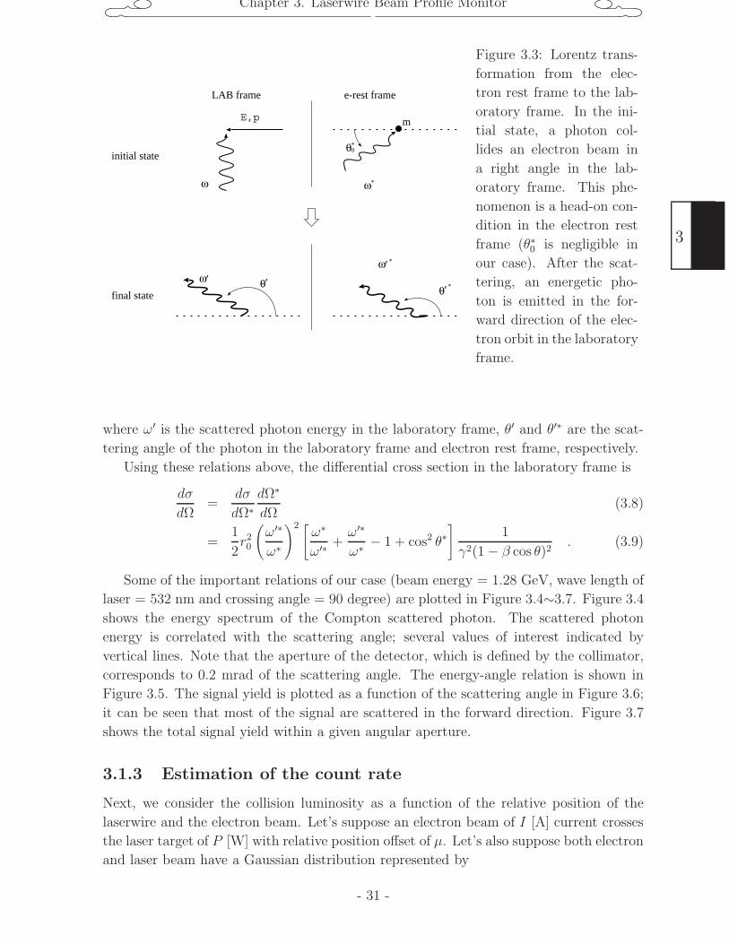
Chapter 3. Laserwire Beam Profile Monitor
ω ω
LAB frame e-rest frame
*
E,p
θ*0
m
ω *
θ *θω’’
’’
final state
initial state
Figure 3.3: Lorentz trans-
formation from the elec-
tron rest frame to the lab-
oratory frame. In the ini-
tial state, a photon col-
lides an electron beam in
a right angle in the lab-
oratory frame. This phe-
nomenon is a head-on con-
dition in the electron rest
frame (θ∗0 is negligible in
our case). After the scat-
tering, an energetic pho-
ton is emitted in the for-
ward direction of the elec-
tron orbit in the laboratory
frame.
where ω′ is the scattered photon energy in the laboratory frame, θ′ and θ′∗ are the scat-
tering angle of the photon in the laboratory frame and electron rest frame, respectively.
Using these relations above, the differential cross section in the laboratory frame is
dσ
dΩ=
dσ
dΩ∗dΩ∗
dΩ(3.8)
=1
2r20
(ω′∗
ω∗
)2 [ω∗
ω′∗ +ω′∗
ω∗ − 1 + cos2 θ∗]
1
γ2(1 − β cos θ)2. (3.9)
Some of the important relations of our case (beam energy = 1.28 GeV, wave length of
laser = 532 nm and crossing angle = 90 degree) are plotted in Figure 3.4∼3.7. Figure 3.4
shows the energy spectrum of the Compton scattered photon. The scattered photon
energy is correlated with the scattering angle; several values of interest indicated by
vertical lines. Note that the aperture of the detector, which is defined by the collimator,
corresponds to 0.2 mrad of the scattering angle. The energy-angle relation is shown in
Figure 3.5. The signal yield is plotted as a function of the scattering angle in Figure 3.6;
it can be seen that most of the signal are scattered in the forward direction. Figure 3.7
shows the total signal yield within a given angular aperture.
3.1.3 Estimation of the count rate
Next, we consider the collision luminosity as a function of the relative position of the
laserwire and the electron beam. Let’s suppose an electron beam of I [A] current crosses
the laser target of P [W] with relative position offset of µ. Let’s also suppose both electron
and laser beam have a Gaussian distribution represented by
- 31 -
3
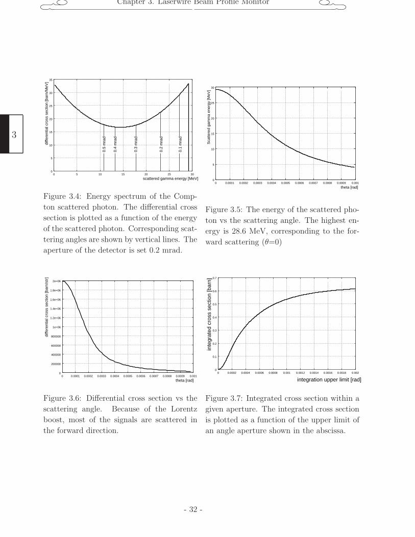
Chapter 3. Laserwire Beam Profile Monitor
0
5
10
15
20
25
30
35
0 5 10 15 20 25 30
scattered gamma energy [MeV]
diffe
rent
ial c
ross
sec
tion
[bar
n/M
eV]
0.1
mra
d
0.2
mra
d
0.3
mra
d
0.4
mra
d
0.5
mra
d
Figure 3.4: Energy spectrum of the Comp-
ton scattered photon. The differential cross
section is plotted as a function of the energy
of the scattered photon. Corresponding scat-
tering angles are shown by vertical lines. The
aperture of the detector is set 0.2 mrad.
0
5
10
15
20
25
30
0 0.0001 0.0002 0.0003 0.0004 0.0005 0.0006 0.0007 0.0008 0.0009 0.001
Sca
ttere
d ga
mm
a en
ergy
[MeV
]
theta [rad]
Figure 3.5: The energy of the scattered pho-
ton vs the scattering angle. The highest en-
ergy is 28.6 MeV, corresponding to the for-
ward scattering (θ=0)
0
200000
400000
600000
800000
1e+06
1.2e+06
1.4e+06
1.6e+06
1.8e+06
2e+06
0 0.0001 0.0002 0.0003 0.0004 0.0005 0.0006 0.0007 0.0008 0.0009 0.001
theta [rad]
diffe
rent
ial c
ross
sec
tion
[bar
n/st
r]
Figure 3.6: Differential cross section vs the
scattering angle. Because of the Lorentz
boost, most of the signals are scattered in
the forward direction.
0
0.1
0.2
0.3
0.4
0.5
0.6
0.7
0 0.0002 0.0004 0.0006 0.0008 0.001 0.0012 0.0014 0.0016 0.0018 0.002
inte
grat
ed c
ross
sec
tion
[bar
n]
integration upper limit [rad]
Figure 3.7: Integrated cross section within a
given aperture. The integrated cross section
is plotted as a function of the upper limit of
an angle aperture shown in the abscissa.
3
- 32 -
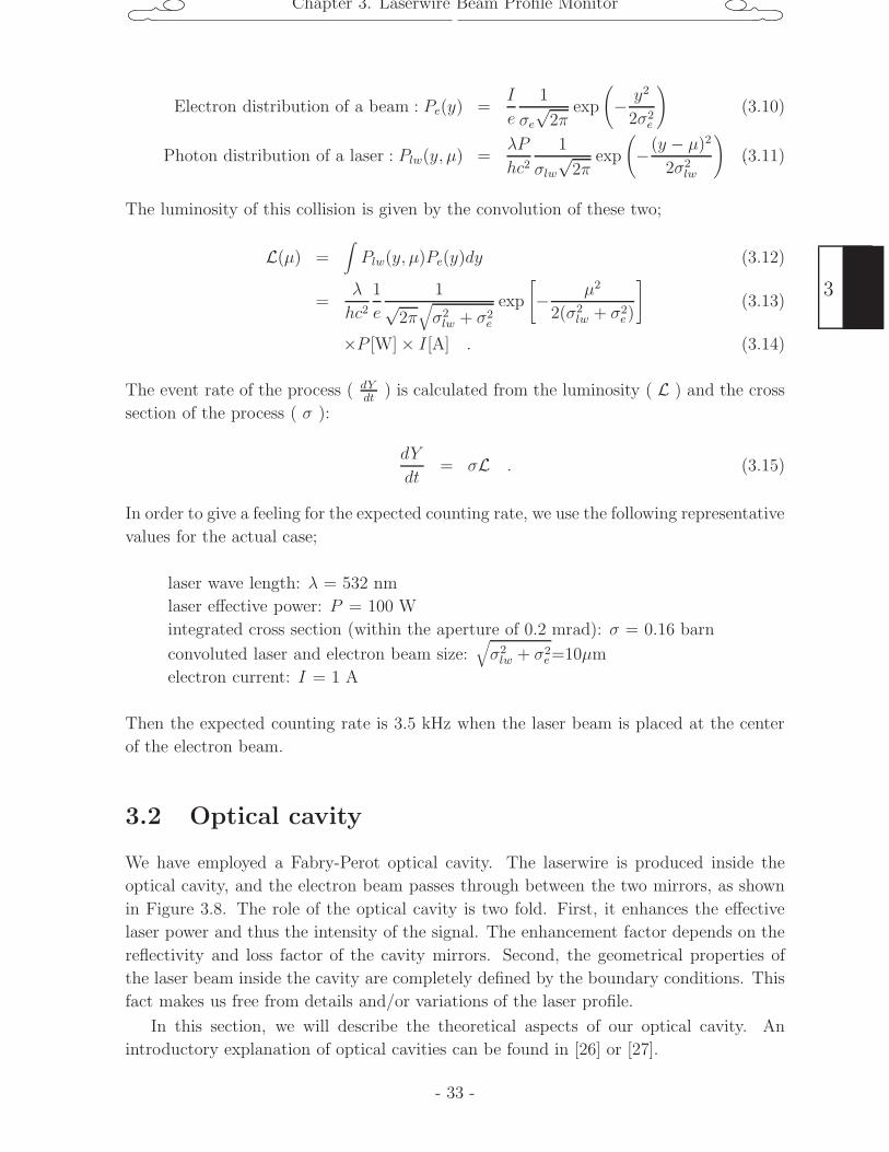
Chapter 3. Laserwire Beam Profile Monitor
Electron distribution of a beam : Pe(y) =I
e
1
σe
√2π
exp
(− y2
2σ2e
)(3.10)
Photon distribution of a laser : Plw(y, µ) =λP
hc21
σlw
√2π
exp
(−(y − µ)2
2σ2lw
).(3.11)
The luminosity of this collision is given by the convolution of these two;
L(µ) =∫Plw(y, µ)Pe(y)dy (3.12)
=λ
hc21
e
1√2π√σ2
lw + σ2e
exp
[− µ2
2(σ2lw + σ2
e)
](3.13)
×P [W] × I[A] . (3.14)
The event rate of the process ( dYdt
) is calculated from the luminosity ( L ) and the cross
section of the process ( σ ):
dY
dt= σL . (3.15)
In order to give a feeling for the expected counting rate, we use the following representative
values for the actual case;
laser wave length: λ = 532 nm
laser effective power: P = 100 W
integrated cross section (within the aperture of 0.2 mrad): σ = 0.16 barn
convoluted laser and electron beam size:√σ2
lw + σ2e=10µm
electron current: I = 1 A
Then the expected counting rate is 3.5 kHz when the laser beam is placed at the center
of the electron beam.
3.2 Optical cavity
We have employed a Fabry-Perot optical cavity. The laserwire is produced inside the
optical cavity, and the electron beam passes through between the two mirrors, as shown
in Figure 3.8. The role of the optical cavity is two fold. First, it enhances the effective
laser power and thus the intensity of the signal. The enhancement factor depends on the
reflectivity and loss factor of the cavity mirrors. Second, the geometrical properties of
the laser beam inside the cavity are completely defined by the boundary conditions. This
fact makes us free from details and/or variations of the laser profile.
In this section, we will describe the theoretical aspects of our optical cavity. An
introductory explanation of optical cavities can be found in [26] or [27].
- 33 -
3
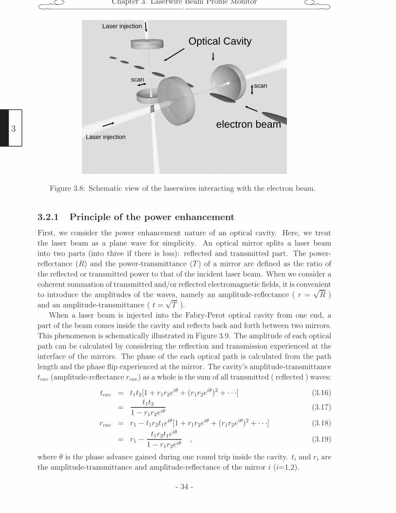
Chapter 3. Laserwire Beam Profile Monitor
Optical Cavity
Laser injection
Laser injection
scanscan
electron beam
Figure 3.8: Schematic view of the laserwires interacting with the electron beam.
3.2.1 Principle of the power enhancement
First, we consider the power enhancement nature of an optical cavity. Here, we treat
the laser beam as a plane wave for simplicity. An optical mirror splits a laser beam
into two parts (into three if there is loss): reflected and transmitted part. The power-
reflectance (R) and the power-transmittance (T ) of a mirror are defined as the ratio of
the reflected or transmitted power to that of the incident laser beam. When we consider a
coherent summation of transmitted and/or reflected electromagnetic fields, it is convenient
to introduce the amplitudes of the waves, namely an amplitude-reflectance ( r =√R )
and an amplitude-transmittance ( t =√T ).
When a laser beam is injected into the Fabry-Perot optical cavity from one end, a
part of the beam comes inside the cavity and reflects back and forth between two mirrors.
This phenomenon is schematically illustrated in Figure 3.9. The amplitude of each optical
path can be calculated by considering the reflection and transmission experienced at the
interface of the mirrors. The phase of the each optical path is calculated from the path
length and the phase flip experienced at the mirror. The cavity’s amplitude-transmittance
tcav (amplitude-reflectance rcav) as a whole is the sum of all transmitted ( reflected ) waves;
tcav = t1t2[1 + r1r2eiθ + (r1r2e
iθ)2 + · · ·] (3.16)
=t1t2
1 − r1r2eiθ(3.17)
rcav = r1 − t1r2t1eiθ[1 + r1r2e
iθ + (r1r2eiθ)2 + · · ·] (3.18)
= r1 − t1r2t1eiθ
1 − r1r2eiθ, (3.19)
where θ is the phase advance gained during one round trip inside the cavity. ti and ri are
the amplitude-transmittance and amplitude-reflectance of the mirror i (i=1,2).
3
- 34 -
Chapter 3. Laserwire Beam Profile Monitor
mirror1 mirror21
rt
t t
t r tt r r t
t r r r t
t r
t r r
t r r r
Injection
Reflection
Transmission
Store
S
S T1
R 12
21
mirror1 mirror2
cav
cav
1
1 2
1 2 1
1 2 1 2
1 2 1 2 1
1 2 1
1
1 2 1 2
1 2
Rcav Tcav
S = + S12 S21
eiθphaseadvance
Figure 3.9: Schematic diagram of the power enhancement in an optical cavity.
The amplitude of the waves inside the cavity can be calculated in the same way. The
amplitude of the wave going from mirror-1 to mirror-2 (s12) and the one going from
mirror-2 to mirror-1 (s21) are
s12 = t1[1 + r1r2eiθ + (r1r2e
iθ)2 + · · ·] (3.20)
=t1
1 − r1r2eiθ(3.21)
s21 = t1r2[1 + r1r2eiθ + (r1r2e
iθ)2 + · · ·] (3.22)
=t1r2
1 − r1r2eiθ. (3.23)
The power-transmittance, the power-reflectance and the power enhancement factor of the
cavity ( Tcav, Rcav and Scav, respectively ) are obtained by squaring respective amplitudes;
Tcav = |tcav|2 =T1T2
(1 −√R1R2)2 + 4
√R1R2 sin2 θ
2
(3.24)
Rcav = |rcav|2 = (R1 + T1) − T1(1 − R1R2 − T1R2)
(1 −√R1R2)2 + 4
√R1R2 sin2 θ
2
(3.25)
Scav = |s12|2 + |s21|2 =T1(1 +R2)
(1 −√R1R2)2 + 4
√R1R2 sin2 θ
2
(3.26)
=1 +R2
T2Tcav ∼ 2
T2Tcav (if R2 ∼ 1) . (3.27)
The phase advance in one round trip, θ (= 2π 2Lλ
), depends on the cavity length and
the wavelength of the light. It is convenient to define a quantity called the resonating
efficiency η, which is basically the denominator of Eq. 3.24-3.26;
η =(1 −√
R1R2)2
(1 −√R1R2)2 + 4
√R1R2 sin2 θ
2
. (3.28)
- 35 -
3
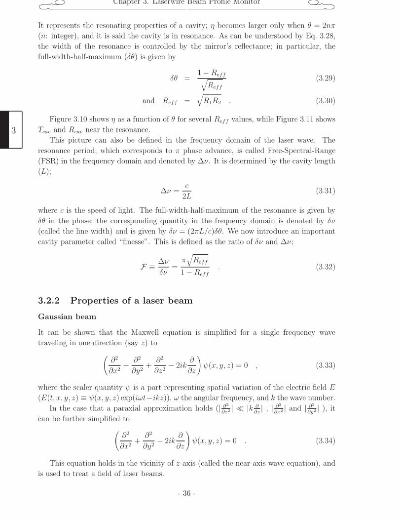
Chapter 3. Laserwire Beam Profile Monitor
It represents the resonating properties of a cavity; η becomes larger only when θ = 2nπ
(n: integer), and it is said the cavity is in resonance. As can be understood by Eq. 3.28,
the width of the resonance is controlled by the mirror’s reflectance; in particular, the
full-width-half-maximum (δθ) is given by
δθ =1 − Reff√
Reff
(3.29)
and Reff =√R1R2 . (3.30)
Figure 3.10 shows η as a function of θ for several Reff values, while Figure 3.11 shows
Tcav and Rcav near the resonance.
This picture can also be defined in the frequency domain of the laser wave. The
resonance period, which corresponds to π phase advance, is called Free-Spectral-Range
(FSR) in the frequency domain and denoted by ∆ν. It is determined by the cavity length
(L);
∆ν =c
2L(3.31)
where c is the speed of light. The full-width-half-maximum of the resonance is given by
δθ in the phase; the corresponding quantity in the frequency domain is denoted by δν
(called the line width) and is given by δν = (2πL/c)δθ. We now introduce an important
cavity parameter called “finesse”. This is defined as the ratio of δν and ∆ν;
F ≡ ∆ν
δν=
π√Reff
1 −Reff. (3.32)
3.2.2 Properties of a laser beam
Gaussian beam
It can be shown that the Maxwell equation is simplified for a single frequency wave
traveling in one direction (say z) to
(∂2
∂x2+
∂2
∂y2+
∂2
∂z2− 2ik
∂
∂z
)ψ(x, y, z) = 0 , (3.33)
where the scaler quantity ψ is a part representing spatial variation of the electric field E
(E(t, x, y, z) ≡ ψ(x, y, z) exp(iωt−ikz)), ω the angular frequency, and k the wave number.
In the case that a paraxial approximation holds (| ∂2
∂z2 | |k ∂∂z| , | ∂2
∂x2 | and | ∂2
∂y2 | ), it
can be further simplified to
(∂2
∂x2+
∂2
∂y2− 2ik
∂
∂z
)ψ(x, y, z) = 0 . (3.34)
This equation holds in the vicinity of z-axis (called the near-axis wave equation), and
is used to treat a field of laser beams.
3
- 36 -
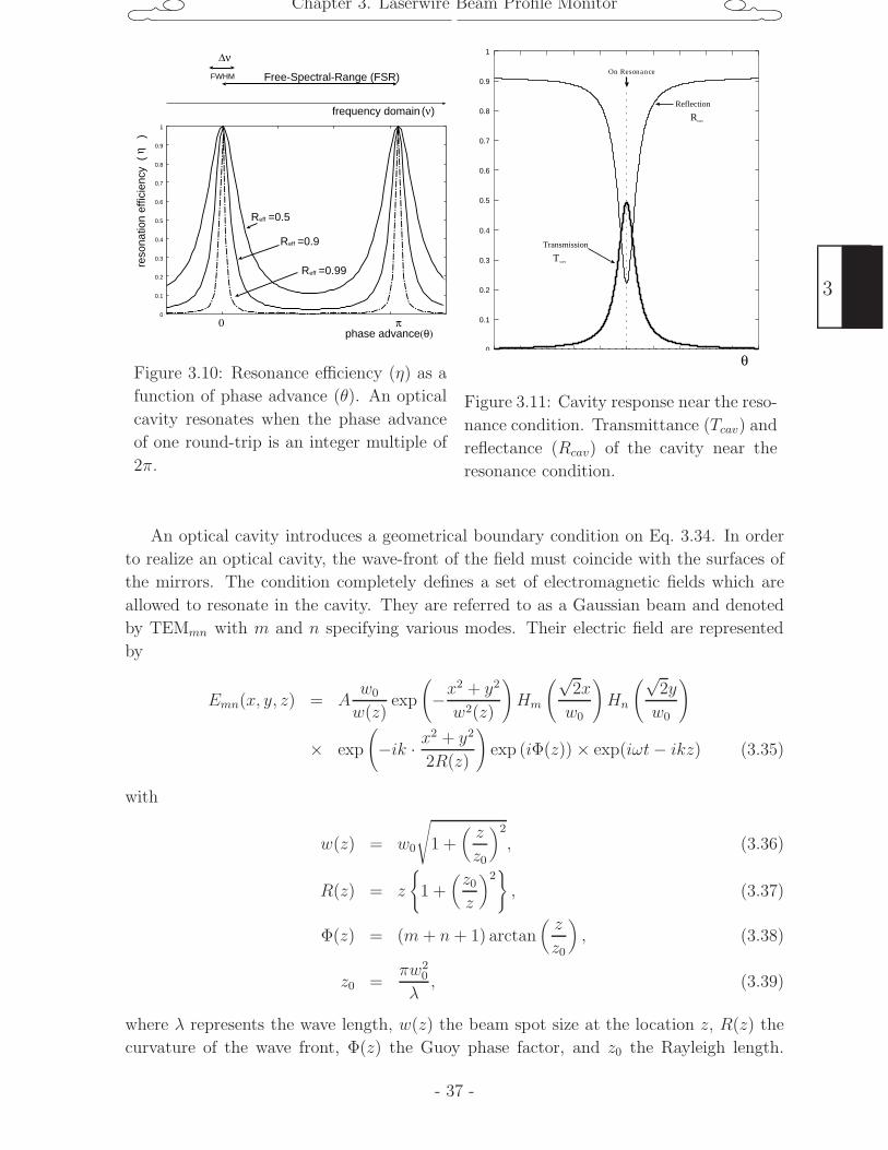
Chapter 3. Laserwire Beam Profile Monitor
0
0.1
0.2
0.3
0.4
0.5
0.6
0.7
0.8
0.9
1
π0
reso
natio
n ef
ficie
ncy
(
)
R =0.5
R =0.9
R =0.99
eff
eff
eff
(θ)
η
Free-Spectral-Range (FSR)
∆ν
frequency domain (ν)
FWHM
phase advance
Figure 3.10: Resonance efficiency (η) as a
function of phase advance (θ). An optical
cavity resonates when the phase advance
of one round-trip is an integer multiple of
2π.
0
0.1
0.2
0.3
0.4
0.5
0.6
0.7
0.8
0.9
1
-1000 -800 -600 -400 -200 400 600 800 1000
T
R
cav
cav
On Resonance
Reflection
Transmission
θ
Figure 3.11: Cavity response near the reso-
nance condition. Transmittance (Tcav) and
reflectance (Rcav) of the cavity near the
resonance condition.
An optical cavity introduces a geometrical boundary condition on Eq. 3.34. In order
to realize an optical cavity, the wave-front of the field must coincide with the surfaces of
the mirrors. The condition completely defines a set of electromagnetic fields which are
allowed to resonate in the cavity. They are referred to as a Gaussian beam and denoted
by TEMmn with m and n specifying various modes. Their electric field are represented
by
Emn(x, y, z) = Aw0
w(z)exp
(−x
2 + y2
w2(z)
)Hm
(√2x
w0
)Hn
(√2y
w0
)
× exp
(−ik · x
2 + y2
2R(z)
)exp (iΦ(z)) × exp(iωt− ikz) (3.35)
with
w(z) = w0
√1 +
(z
z0
)2
, (3.36)
R(z) = z
1 +
(z0z
)2, (3.37)
Φ(z) = (m + n+ 1) arctan(z
z0
), (3.38)
z0 =πw2
0
λ, (3.39)
where λ represents the wave length, w(z) the beam spot size at the location z, R(z) the
curvature of the wave front, Φ(z) the Guoy phase factor, and z0 the Rayleigh length.
- 37 -
3
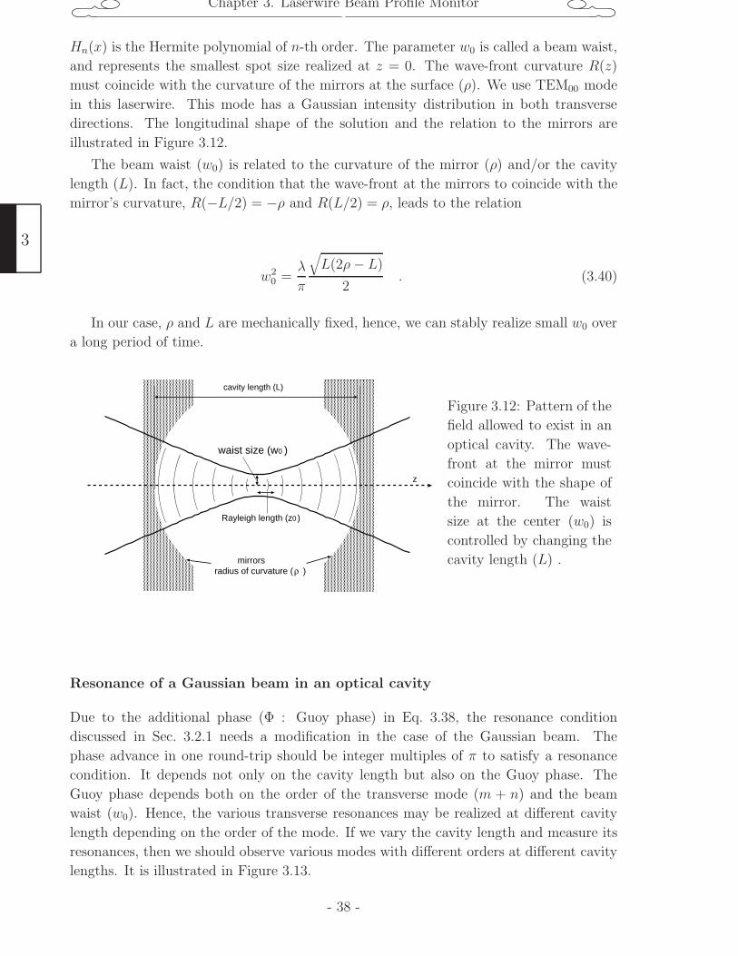
Chapter 3. Laserwire Beam Profile Monitor
Hn(x) is the Hermite polynomial of n-th order. The parameter w0 is called a beam waist,
and represents the smallest spot size realized at z = 0. The wave-front curvature R(z)
must coincide with the curvature of the mirrors at the surface (ρ). We use TEM00 mode
in this laserwire. This mode has a Gaussian intensity distribution in both transverse
directions. The longitudinal shape of the solution and the relation to the mirrors are
illustrated in Figure 3.12.
The beam waist (w0) is related to the curvature of the mirror (ρ) and/or the cavity
length (L). In fact, the condition that the wave-front at the mirrors to coincide with the
mirror’s curvature, R(−L/2) = −ρ and R(L/2) = ρ, leads to the relation
w20 =
λ
π
√L(2ρ− L)
2. (3.40)
In our case, ρ and L are mechanically fixed, hence, we can stably realize small w0 over
a long period of time.
cavity length (L)
waist size (w )0
Rayleigh length (z )0
z
radius of curvature ( )ρmirrors
Figure 3.12: Pattern of the
field allowed to exist in an
optical cavity. The wave-
front at the mirror must
coincide with the shape of
the mirror. The waist
size at the center (w0) is
controlled by changing the
cavity length (L) .
Resonance of a Gaussian beam in an optical cavity
Due to the additional phase (Φ : Guoy phase) in Eq. 3.38, the resonance condition
discussed in Sec. 3.2.1 needs a modification in the case of the Gaussian beam. The
phase advance in one round-trip should be integer multiples of π to satisfy a resonance
condition. It depends not only on the cavity length but also on the Guoy phase. The
Guoy phase depends both on the order of the transverse mode (m + n) and the beam
waist (w0). Hence, the various transverse resonances may be realized at different cavity
length depending on the order of the mode. If we vary the cavity length and measure its
resonances, then we should observe various modes with different orders at different cavity
lengths. It is illustrated in Figure 3.13.
3
- 38 -
Chapter 3. Laserwire Beam Profile Monitor
reso
natio
n 0th
1st
2nd3rd
π θ
Figure 3.13: Resonance
conditions of various trans-
verse modes. The cav-
ity length which satis-
fies the resonance condi-
tion depends on the order
(m+n) of the modes. They
appears as sub-peaks when
the cavity length is swept.
3.3 Experimental setup
3.3.1 Layout
The experimental layout is shown in Figure 3.14. Two laserwires were installed in
the north straight section of the damping ring. One is to measure vertical beam size
(horizontal-wire) and the other to measure horizontal one (vertical-wire). The electron
beam passes through from right to left at the interaction points. A photon detector was
placed 12.7 m downstream of the vertical-wire. We designed the interaction points to be
placed in the straight section of the ring. This made the emittance measurement free from
the effects of the momentum dispersion. From the view point of detector backgrounds,
however, this configuration had a disadvantage. Backgrounds were mainly caused by
γ-rays which were in turn stemmed from beam loss of the spent electrons and beam scat-
tering with residual gases. They tended to come along the beam, and thus most of the
backgrounds generated in the whole north-straight section came into the detector. This
problem was partly cured by placing collimators in front of the detector.
3.3.2 Optical system
Cavity assembly and the chamber system
The cavity and other related components were structured into one assembly called a
cavity assembly. The cavity itself was composed of two spherical mirrors with the same
curvature of ρ = 20 mm; they were apart by L 40 mm. The optical properties of the
cavities will be detailed in Sec. 3.3.3. The cavity assembly consisted of two mirrors, mirror
holder systems and a cylindrical spacer which defined the cavity length. In order to have
precision control over the cavity length, both mirror holders were supported by a piezo
actuator through a disk-type plate spring. The piezo actuators had a hollow to let a laser
beam go through. The mechanical resonance frequency of the plate spring was found to
be around 6 kHz. It limited the bandwidth of the feedback control on the cavity length.
There were two sets of cavity assemblies: one for the horizontal-wire and the other for
the vertical one. They were mostly identical, but were placed in orthogonal. They were
mounted in a vacuum chamber as shown in Figure 3.15. The laser beam was injected
- 39 -
3
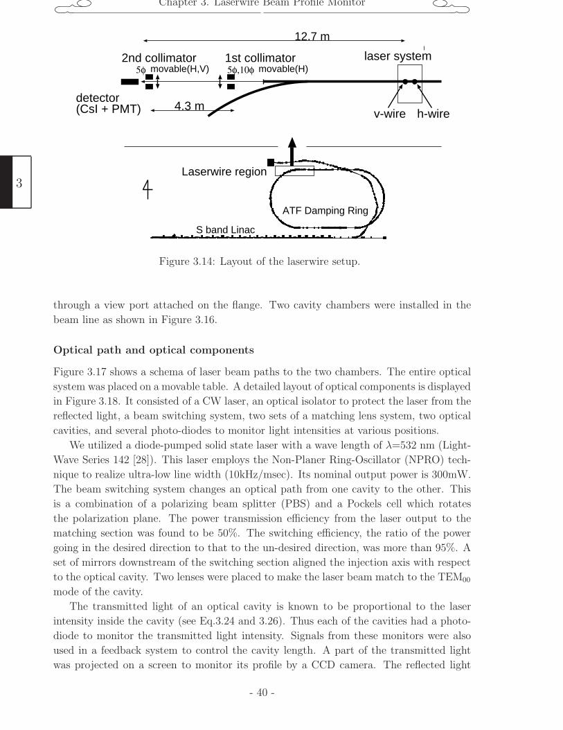
Chapter 3. Laserwire Beam Profile Monitor
detector
1st collimator2nd collimator5φ 5φ,10φ
12.7 m
4.3 m
movable(H,V) movable(H)
(CsI + PMT)
Laserwire region
ATF Damping Ring
S band Linac
laser system
h-wirev-wire
Figure 3.14: Layout of the laserwire setup.
through a view port attached on the flange. Two cavity chambers were installed in the
beam line as shown in Figure 3.16.
Optical path and optical components
Figure 3.17 shows a schema of laser beam paths to the two chambers. The entire optical
system was placed on a movable table. A detailed layout of optical components is displayed
in Figure 3.18. It consisted of a CW laser, an optical isolator to protect the laser from the
reflected light, a beam switching system, two sets of a matching lens system, two optical
cavities, and several photo-diodes to monitor light intensities at various positions.
We utilized a diode-pumped solid state laser with a wave length of λ=532 nm (Light-
Wave Series 142 [28]). This laser employs the Non-Planer Ring-Oscillator (NPRO) tech-
nique to realize ultra-low line width (10kHz/msec). Its nominal output power is 300mW.
The beam switching system changes an optical path from one cavity to the other. This
is a combination of a polarizing beam splitter (PBS) and a Pockels cell which rotates
the polarization plane. The power transmission efficiency from the laser output to the
matching section was found to be 50%. The switching efficiency, the ratio of the power
going in the desired direction to that to the un-desired direction, was more than 95%. A
set of mirrors downstream of the switching section aligned the injection axis with respect
to the optical cavity. Two lenses were placed to make the laser beam match to the TEM00
mode of the cavity.
The transmitted light of an optical cavity is known to be proportional to the laser
intensity inside the cavity (see Eq.3.24 and 3.26). Thus each of the cavities had a photo-
diode to monitor the transmitted light intensity. Signals from these monitors were also
used in a feedback system to control the cavity length. A part of the transmitted light
was projected on a screen to monitor its profile by a CCD camera. The reflected light
3
- 40 -
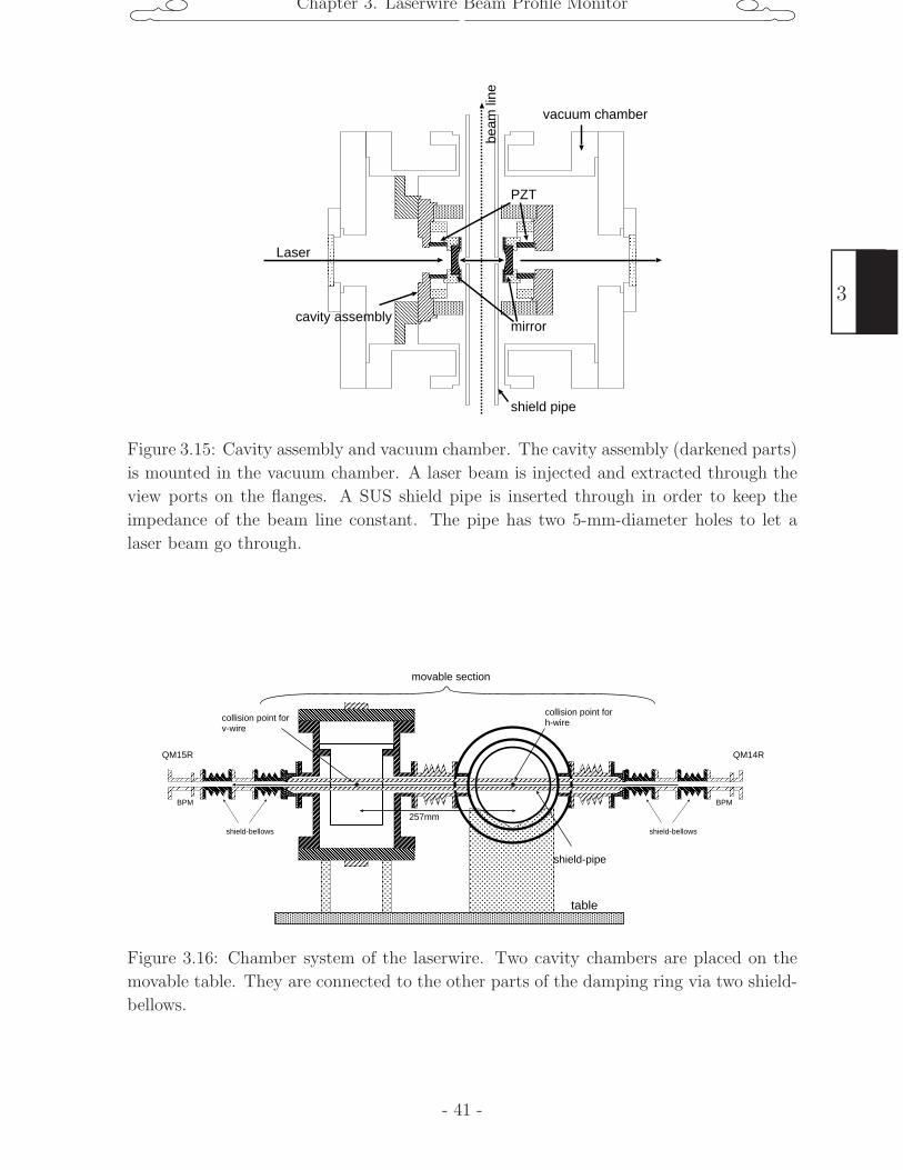
Chapter 3. Laserwire Beam Profile Monitor
beam
line
Laser
cavity assemblymirror
PZT
vacuum chamber
shield pipe
Figure 3.15: Cavity assembly and vacuum chamber. The cavity assembly (darkened parts)
is mounted in the vacuum chamber. A laser beam is injected and extracted through the
view ports on the flanges. A SUS shield pipe is inserted through in order to keep the
impedance of the beam line constant. The pipe has two 5-mm-diameter holes to let a
laser beam go through.
257mm
QM14RQM15R
table
collision point forh-wirecollision point for
v-wire
shield-pipe
movable section
BPM BPM
shield-bellows shield-bellows
Figure 3.16: Chamber system of the laserwire. Two cavity chambers are placed on the
movable table. They are connected to the other parts of the damping ring via two shield-
bellows.
- 41 -
3
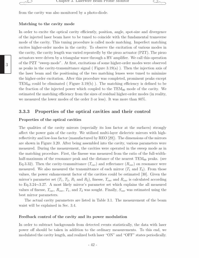
Chapter 3. Laserwire Beam Profile Monitor
from the cavity was also monitored by a photo-diode.
Matching to the cavity mode
In order to excite the optical cavity efficiently, position, angle, spot-size and divergence
of the injected laser beam have to be tuned to coincide with the fundamental transverse
mode of the cavity. This tuning procedure is called mode matching. Imperfect matching
excites higher-order modes in the cavity. To observe the excitation of various modes in
the cavity, the cavity length was varied repeatedly by the piezo actuator (PZT). The piezo
actuators were driven by a triangular wave through a HV amplifier. We call this operation
of the PZT “sweep mode”. At first, excitations of some higher-order modes were observed
as peaks in the cavity-transmittance signal ( Figure 3.19(a) ). Then the injection axis of
the laser beam and the positioning of the two matching lenses were tuned to minimize
the higher-order excitation. After this procedure was completed, prominent peaks except
TEM00 could be eliminated ( Figure 3.19(b) ). The matching efficiency is defined to be
the fraction of the injected power which coupled to the TEM00 mode of the cavity. We
estimated the matching efficiency from the sizes of residual higher-order modes (in reality,
we measured the lower modes of the order 3 or less). It was more than 80%.
3.3.3 Properties of the optical cavities and their control
Properties of the optical cavities
The qualities of the cavity mirrors (especially its loss factor at the surfaces) strongly
affect the power gain of the cavity. We utilized multi-layer dielectric mirrors with high-
reflectivity and low-loss factor (manufactured by REO [29]). The dimensions of the mirrors
are shown in Figure 3.20. After being assembled into the cavity, various parameters were
measured. During the measurement, the cavities were operated in the sweep mode as in
the matching procedure. First, the finesse was measured from the ratio of the full-width-
half-maximum of the resonance peak and the distance of the nearest TEM00 peaks. (see
Eq.3.32). Then the cavity-transmittance (Tcav) and reflectance (Rcav) on resonance were
measured. We also measured the transmittance of each mirror (T1 and T2). From those
values, the power enhancement factor of the cavities could be estimated [30]. Given the
mirror’s parameter set (T1, T2, R1 and R2), finesse, Tcav and Rcav is calculated according
to Eq.3.24∼3.27. A most likely mirror’s parameter set which explains the all measured
values of finesse, Tcav, Rcav, T1, and T2 was sought. Finally, Scav was estimated using the
best mirror parameters.
The actual cavity parameters are listed in Table 3.1. The measurement of the beam
waist will be explained in Sec. 3.4.
Feedback control of the cavity and its power modulation
In order to subtract backgrounds from detected events statistically, the data with laser
power off should be taken in addition to the ordinary measurements. To this end, we
modulated the cavity length, and realized both laser “ON” and “OFF” states periodically.
3
- 42 -
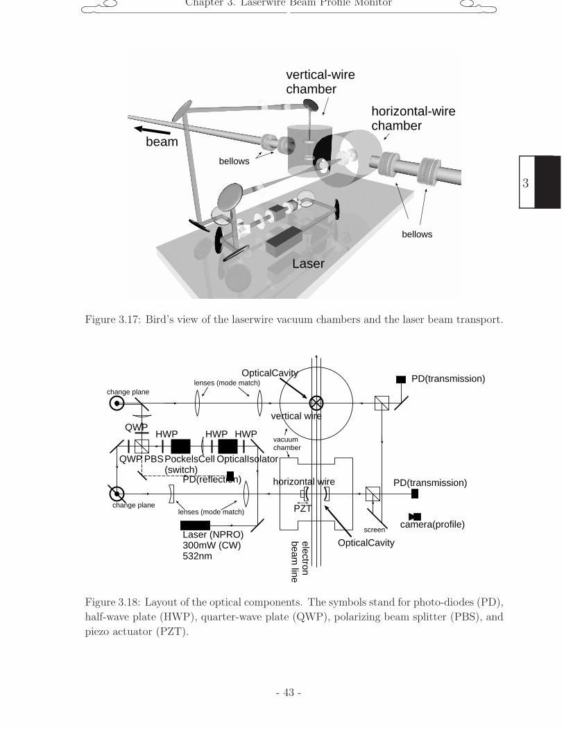
Chapter 3. Laserwire Beam Profile Monitor
horizontal-wirechamber
vertical-wirechamber
Laser
bellows
bellows
beam
Figure 3.17: Bird’s view of the laserwire vacuum chambers and the laser beam transport.
electron beam
line
Laser (NPRO)300mW (CW)532nm
screencamera(profile)
PZT
QWP
HWP HWP
OpticalIsolator
PD(transmission)
vacuumchamber
OpticalCavity
lenses (mode match)
PBS
HWP
PockelsCell(switch)
QWP
PD(transmission)OpticalCavity
horizontal wire
vertical wire
change plane
change plane
lenses (mode match)
PD(reflection)
Figure 3.18: Layout of the optical components. The symbols stand for photo-diodes (PD),
half-wave plate (HWP), quarter-wave plate (QWP), polarizing beam splitter (PBS), and
piezo actuator (PZT).
- 43 -
3
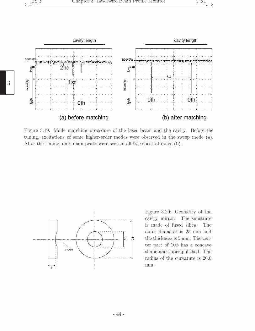
Chapter 3. Laserwire Beam Profile Monitor
(a) before matching (b) after matching
pedestal
inte
nsity
high
low
0th0th
λ/2
pedestal
inte
nsity
high
low
0th
1st
2nd
cavity length cavity length
Figure 3.19: Mode matching procedure of the laser beam and the cavity. Before the
tuning, excitations of some higher-order modes were observed in the sweep mode (a).
After the tuning, only main peaks were seen in all free-spectral-range (b).
10 25
ρ=20.0
5
Figure 3.20: Geometry of the
cavity mirror. The substrate
is made of fused silica. The
outer diameter is 25 mm and
the thickness is 5 mm. The cen-
ter part of 10φ has a concave
shape and super-polished. The
radius of the curvature is 20.0
mm.
3
- 44 -
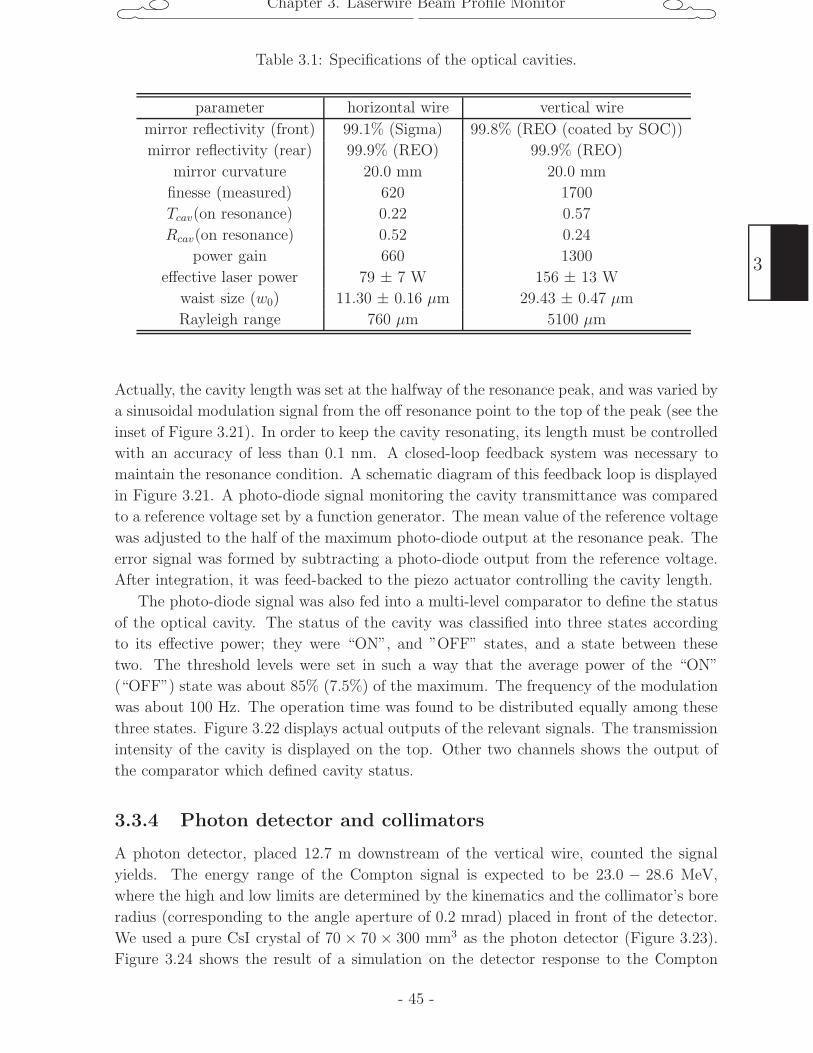
Chapter 3. Laserwire Beam Profile Monitor
Table 3.1: Specifications of the optical cavities.
parameter horizontal wire vertical wire
mirror reflectivity (front) 99.1% (Sigma) 99.8% (REO (coated by SOC))
mirror reflectivity (rear) 99.9% (REO) 99.9% (REO)
mirror curvature 20.0 mm 20.0 mm
finesse (measured) 620 1700
Tcav(on resonance) 0.22 0.57
Rcav(on resonance) 0.52 0.24
power gain 660 1300
effective laser power 79 ± 7 W 156 ± 13 W
waist size (w0) 11.30 ± 0.16 µm 29.43 ± 0.47 µm
Rayleigh range 760 µm 5100 µm
Actually, the cavity length was set at the halfway of the resonance peak, and was varied by
a sinusoidal modulation signal from the off resonance point to the top of the peak (see the
inset of Figure 3.21). In order to keep the cavity resonating, its length must be controlled
with an accuracy of less than 0.1 nm. A closed-loop feedback system was necessary to
maintain the resonance condition. A schematic diagram of this feedback loop is displayed
in Figure 3.21. A photo-diode signal monitoring the cavity transmittance was compared
to a reference voltage set by a function generator. The mean value of the reference voltage
was adjusted to the half of the maximum photo-diode output at the resonance peak. The
error signal was formed by subtracting a photo-diode output from the reference voltage.
After integration, it was feed-backed to the piezo actuator controlling the cavity length.
The photo-diode signal was also fed into a multi-level comparator to define the status
of the optical cavity. The status of the cavity was classified into three states according
to its effective power; they were “ON”, and ”OFF” states, and a state between these
two. The threshold levels were set in such a way that the average power of the “ON”
(“OFF”) state was about 85% (7.5%) of the maximum. The frequency of the modulation
was about 100 Hz. The operation time was found to be distributed equally among these
three states. Figure 3.22 displays actual outputs of the relevant signals. The transmission
intensity of the cavity is displayed on the top. Other two channels shows the output of
the comparator which defined cavity status.
3.3.4 Photon detector and collimators
A photon detector, placed 12.7 m downstream of the vertical wire, counted the signal
yields. The energy range of the Compton signal is expected to be 23.0 − 28.6 MeV,
where the high and low limits are determined by the kinematics and the collimator’s bore
radius (corresponding to the angle aperture of 0.2 mrad) placed in front of the detector.
We used a pure CsI crystal of 70 × 70 × 300 mm3 as the photon detector (Figure 3.23).
Figure 3.24 shows the result of a simulation on the detector response to the Compton
- 45 -
3
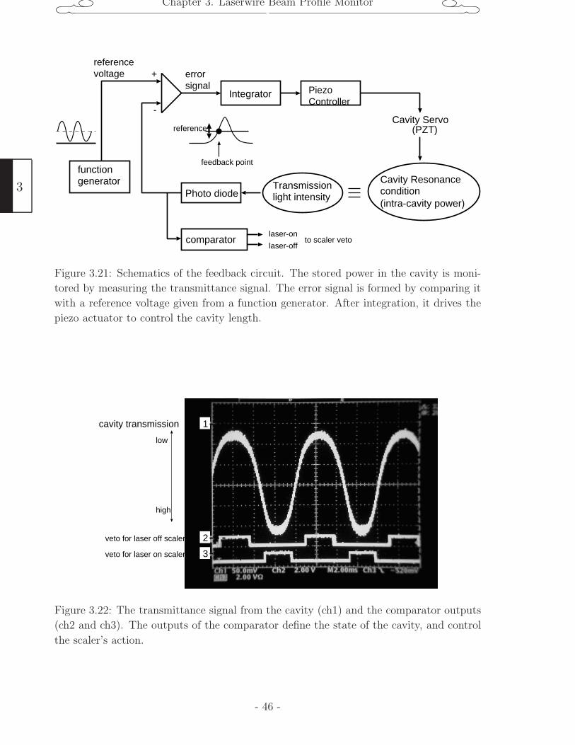
Chapter 3. Laserwire Beam Profile Monitor
Integrator PiezoController
Cavity Servo(PZT)
Cavity ResonanceconditionTransmission
light intensity(intra-cavity power)
Photo diode
+
-
errorsignal
referencevoltage
functiongenerator
reference
feedback point
comparatorlaser-on
laser-offto scaler veto
Figure 3.21: Schematics of the feedback circuit. The stored power in the cavity is moni-
tored by measuring the transmittance signal. The error signal is formed by comparing it
with a reference voltage given from a function generator. After integration, it drives the
piezo actuator to control the cavity length.
1
2
3
cavity transmission
veto for laser off scaler
veto for laser on scaler
low
high
Figure 3.22: The transmittance signal from the cavity (ch1) and the comparator outputs
(ch2 and ch3). The outputs of the comparator define the state of the cavity, and control
the scaler’s action.
3
- 46 -
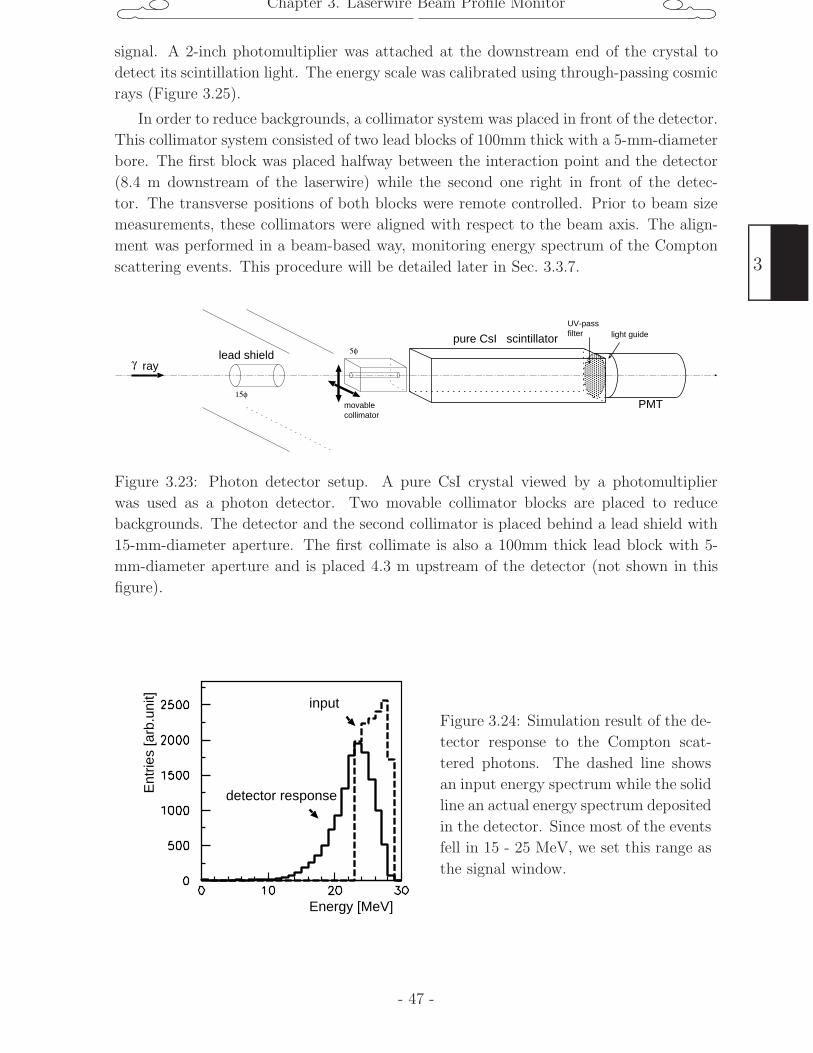
Chapter 3. Laserwire Beam Profile Monitor
signal. A 2-inch photomultiplier was attached at the downstream end of the crystal to
detect its scintillation light. The energy scale was calibrated using through-passing cosmic
rays (Figure 3.25).
In order to reduce backgrounds, a collimator system was placed in front of the detector.
This collimator system consisted of two lead blocks of 100mm thick with a 5-mm-diameter
bore. The first block was placed halfway between the interaction point and the detector
(8.4 m downstream of the laserwire) while the second one right in front of the detec-
tor. The transverse positions of both blocks were remote controlled. Prior to beam size
measurements, these collimators were aligned with respect to the beam axis. The align-
ment was performed in a beam-based way, monitoring energy spectrum of the Compton
scattering events. This procedure will be detailed later in Sec. 3.3.7.
movablecollimator
5φpure CsI scintillator
15φ
lead shield
PMT
UV-passfilter light guide
rayγ
Figure 3.23: Photon detector setup. A pure CsI crystal viewed by a photomultiplier
was used as a photon detector. Two movable collimator blocks are placed to reduce
backgrounds. The detector and the second collimator is placed behind a lead shield with
15-mm-diameter aperture. The first collimate is also a 100mm thick lead block with 5-
mm-diameter aperture and is placed 4.3 m upstream of the detector (not shown in this
figure).
Energy [MeV]
Ent
ries
[arb
.uni
t] input
detector response
Figure 3.24: Simulation result of the de-
tector response to the Compton scat-
tered photons. The dashed line shows
an input energy spectrum while the solid
line an actual energy spectrum deposited
in the detector. Since most of the events
fell in 15 - 25 MeV, we set this range as
the signal window.
- 47 -
3
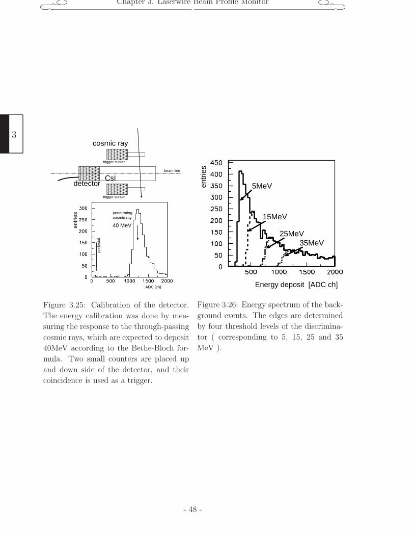
Chapter 3. Laserwire Beam Profile Monitor
trigger cunter
trigger cunter
beam line
CsIdetector
cosmic ray
pede
stal
penetratingcosmic-ray
40 MeV
ADC [ch]
entr
ies
Figure 3.25: Calibration of the detector.
The energy calibration was done by mea-
suring the response to the through-passing
cosmic rays, which are expected to deposit
40MeV according to the Bethe-Bloch for-
mula. Two small counters are placed up
and down side of the detector, and their
coincidence is used as a trigger.
Energy deposit [ADC ch]
entr
ies
5MeV
15MeV
25MeV35MeV
Figure 3.26: Energy spectrum of the back-
ground events. The edges are determined
by four threshold levels of the discrimina-
tor ( corresponding to 5, 15, 25 and 35
MeV ).
3
- 48 -
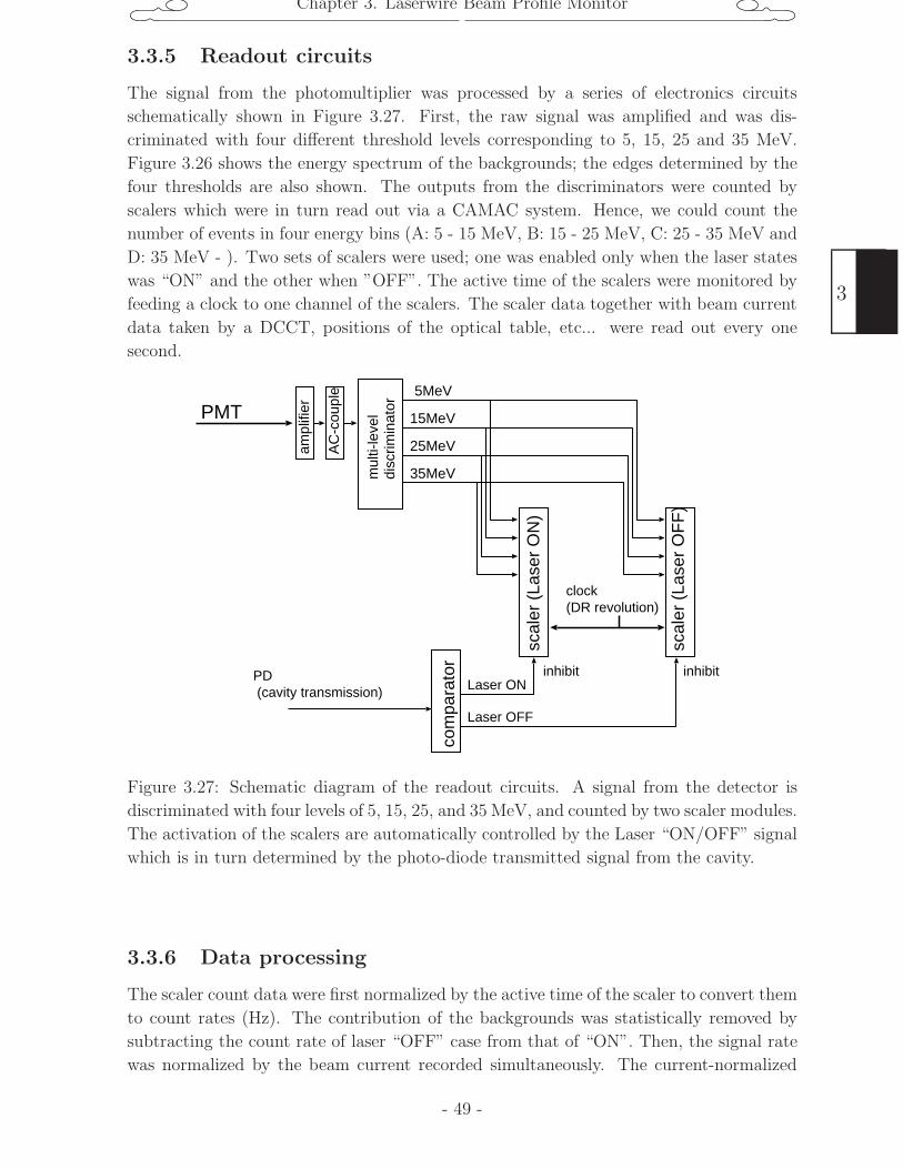
Chapter 3. Laserwire Beam Profile Monitor
3.3.5 Readout circuits
The signal from the photomultiplier was processed by a series of electronics circuits
schematically shown in Figure 3.27. First, the raw signal was amplified and was dis-
criminated with four different threshold levels corresponding to 5, 15, 25 and 35 MeV.
Figure 3.26 shows the energy spectrum of the backgrounds; the edges determined by the
four thresholds are also shown. The outputs from the discriminators were counted by
scalers which were in turn read out via a CAMAC system. Hence, we could count the
number of events in four energy bins (A: 5 - 15 MeV, B: 15 - 25 MeV, C: 25 - 35 MeV and
D: 35 MeV - ). Two sets of scalers were used; one was enabled only when the laser states
was “ON” and the other when ”OFF”. The active time of the scalers were monitored by
feeding a clock to one channel of the scalers. The scaler data together with beam current
data taken by a DCCT, positions of the optical table, etc... were read out every one
second.
scal
er (
Lase
r O
N)
scal
er (
Lase
r O
FF
)PD (cavity transmission)
com
para
tor
inhibit inhibitLaser ON
Laser OFF
mul
ti-le
vel
disc
rimin
atorPMT
AC
-cou
ple
ampl
ifier
5MeV
clock(DR revolution)
15MeV
25MeV
35MeV
Figure 3.27: Schematic diagram of the readout circuits. A signal from the detector is
discriminated with four levels of 5, 15, 25, and 35 MeV, and counted by two scaler modules.
The activation of the scalers are automatically controlled by the Laser “ON/OFF” signal
which is in turn determined by the photo-diode transmitted signal from the cavity.
3.3.6 Data processing
The scaler count data were first normalized by the active time of the scaler to convert them
to count rates (Hz). The contribution of the backgrounds was statistically removed by
subtracting the count rate of laser “OFF” case from that of “ON”. Then, the signal rate
was normalized by the beam current recorded simultaneously. The current-normalized
- 49 -
3
Chapter 3. Laserwire Beam Profile Monitor
signal rate (Hz/mA) obtained in the process above was used to plot the beam profile.
3.3.7 Setup procedure of the detector system
Prior to the beam size measurement, the collimator blocks were aligned in a beam-based-
way. At first, the laser and electron beam collision was established. Monitoring the
count rate both laser “ON” and “OFF”, signal enhancement of laser “ON” was sought by
scanning the position of the laserwire. In this step, no collimators was inserted in the beam
line. Figure 3.28 shows an example of the count rate profile when the laserwire was placed
on the center of the beam position. A ∼ D represent the four different energy bins of the
discriminator. A clear enhancement of the count rate is seen in the energy bin B , where
the Compton signal is expected. Then, alignment procedure of the collimator system
started. The 2nd collimator block (the one right in front of the detector) was inserted
and aligned by monitoring the energy spectrum (Figure 3.29 and Figure 3.30 show the
count rate profiles before and after this procedure.) After that, the 1st collimator was
inserted. Figure 3.31 shows a typical count rate profile after all these procedures were
completed.
Figure 3.32 and 3.33 are the data when the laserwire was placed at the center of the
beam (on beam) and off the beam (off beam), respectively. The data were taken for
the beam current up to 2mA, and were classified into 4 energy bins. As can be clearly
seen, the laser “ON” data significantly differs only when the laserwire is on the beam
(Figure 3.32) and for the energy bin B. Figure 3.34 shows an energy spectrum (the count
rate vs 4 energy bins) for the “on beam” and “off beam” cases. As expected, the signal
is seen only in the B bin of the “on beam” data.
3.3.8 Scanning and data taking system
One run was defined to be one complete round trip from one position of an electron beam
to another, and back to the original position. The scanning was computer controlled and
automated. The stepping motors of the table mover were controlled by a computer via
GPIB connection. For the vertical scan, the data taking time was 10 second long per
point at 10 µm interval. For the horizontal scan, it was 30 second long at every 50 µm. It
took about 6 minutes to obtain one profile for the vertical beam size measurement, and
15 minutes for the horizontal.
3.4 Measurement of the beam waist
The laser beam waist is an important parameter in extracting an electron beam size. We
developed three different methods to measure this value. They are the beam divergence
method, transverse mode difference method and waist scan by an electron beam, and are
described below.
3
- 50 -
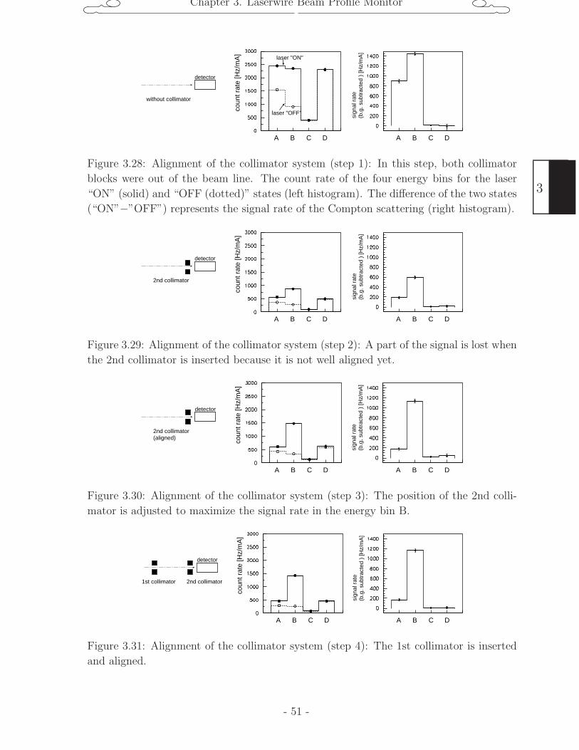
Chapter 3. Laserwire Beam Profile Monitor
coun
t rat
e [H
z/m
A]
sign
al r
ate
(b.g
. sub
trac
ted
) [H
z/m
A]
A B C D A B C D
laser "OFF"
laser "ON"
detector
without collimator
Figure 3.28: Alignment of the collimator system (step 1): In this step, both collimator
blocks were out of the beam line. The count rate of the four energy bins for the laser
“ON” (solid) and “OFF (dotted)” states (left histogram). The difference of the two states
(“ON”−”OFF”) represents the signal rate of the Compton scattering (right histogram).
coun
t rat
e [H
z/m
A]
sign
al r
ate
(b.g
. sub
trac
ted
) [H
z/m
A]
A B C D A B C D
detector
2nd collimator
Figure 3.29: Alignment of the collimator system (step 2): A part of the signal is lost when
the 2nd collimator is inserted because it is not well aligned yet.
coun
t rat
e [H
z/m
A]
sign
al r
ate
(b.g
. sub
trac
ted
) [H
z/m
A]
A B C D A B C D
detector
2nd collimator (aligned)
Figure 3.30: Alignment of the collimator system (step 3): The position of the 2nd colli-
mator is adjusted to maximize the signal rate in the energy bin B.
coun
t rat
e [H
z/m
A]
sign
al r
ate
(b.g
. sub
trac
ted
) [H
z/m
A]
A B C D A B C D
detector
2nd collimator 1st collimator
Figure 3.31: Alignment of the collimator system (step 4): The 1st collimator is inserted
and aligned.
- 51 -
3
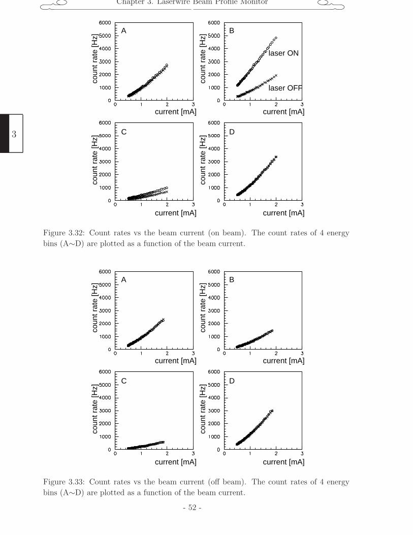
Chapter 3. Laserwire Beam Profile Monitor
current [mA] current [mA]
current [mA] current [mA]
coun
t rat
e [H
z]co
unt r
ate
[Hz]
A B
C D
laser ON
laser OFF
coun
t rat
e [H
z]co
unt r
ate
[Hz]
Figure 3.32: Count rates vs the beam current (on beam). The count rates of 4 energy
bins (A∼D) are plotted as a function of the beam current.
current [mA] current [mA]
current [mA] current [mA]
coun
t rat
e [H
z]co
unt r
ate
[Hz]
coun
t rat
e [H
z]co
unt r
ate
[Hz]
A B
C D
Figure 3.33: Count rates vs the beam current (off beam). The count rates of 4 energy
bins (A∼D) are plotted as a function of the beam current.
3
- 52 -
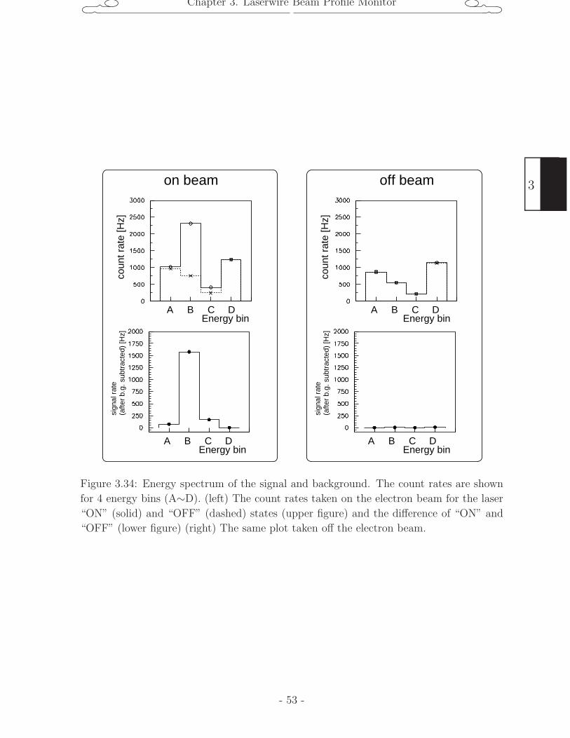
Chapter 3. Laserwire Beam Profile Monitor
A B C DEnergy bin
coun
t rat
e [H
z]si
gnal
rat
e(a
fter
b.g.
sub
trac
ted)
[Hz]
A B C DEnergy bin
A B C D
coun
t rat
e [H
z]si
gnal
rat
e(a
fter
b.g.
sub
trac
ted)
[Hz]
A B C DEnergy bin
Energy bin
on beam off beam
Figure 3.34: Energy spectrum of the signal and background. The count rates are shown
for 4 energy bins (A∼D). (left) The count rates taken on the electron beam for the laser
“ON” (solid) and “OFF” (dashed) states (upper figure) and the difference of “ON” and
“OFF” (lower figure) (right) The same plot taken off the electron beam.
- 53 -
3
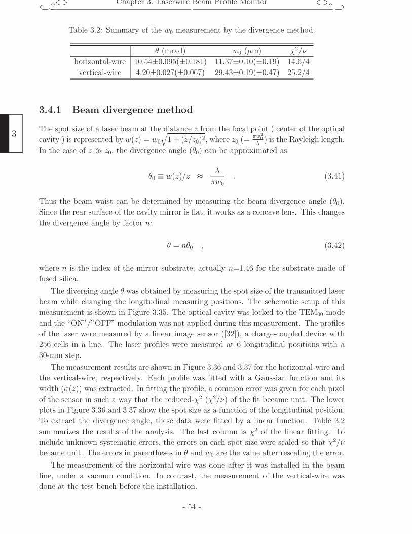
Chapter 3. Laserwire Beam Profile Monitor
Table 3.2: Summary of the w0 measurement by the divergence method.
θ (mrad) w0 (µm) χ2/ν
horizontal-wire 10.54±0.095(±0.181) 11.37±0.10(±0.19) 14.6/4
vertical-wire 4.20±0.027(±0.067) 29.43±0.19(±0.47) 25.2/4
3.4.1 Beam divergence method
The spot size of a laser beam at the distance z from the focal point ( center of the optical
cavity ) is represented by w(z) = w0
√1 + (z/z0)2, where z0 (=
πw20
λ) is the Rayleigh length.
In the case of z z0, the divergence angle (θ0) can be approximated as
θ0 ≡ w(z)/z ≈ λ
πw0. (3.41)
Thus the beam waist can be determined by measuring the beam divergence angle (θ0).
Since the rear surface of the cavity mirror is flat, it works as a concave lens. This changes
the divergence angle by factor n:
θ = nθ0 , (3.42)
where n is the index of the mirror substrate, actually n=1.46 for the substrate made of
fused silica.
The diverging angle θ was obtained by measuring the spot size of the transmitted laser
beam while changing the longitudinal measuring positions. The schematic setup of this
measurement is shown in Figure 3.35. The optical cavity was locked to the TEM00 mode
and the “ON”/”OFF” modulation was not applied during this measurement. The profiles
of the laser were measured by a linear image sensor ([32]), a charge-coupled device with
256 cells in a line. The laser profiles were measured at 6 longitudinal positions with a
30-mm step.
The measurement results are shown in Figure 3.36 and 3.37 for the horizontal-wire and
the vertical-wire, respectively. Each profile was fitted with a Gaussian function and its
width (σ(z)) was extracted. In fitting the profile, a common error was given for each pixel
of the sensor in such a way that the reduced-χ2 (χ2/ν) of the fit became unit. The lower
plots in Figure 3.36 and 3.37 show the spot size as a function of the longitudinal position.
To extract the divergence angle, these data were fitted by a linear function. Table 3.2
summarizes the results of the analysis. The last column is χ2 of the linear fitting. To
include unknown systematic errors, the errors on each spot size were scaled so that χ2/ν
became unit. The errors in parentheses in θ and w0 are the value after rescaling the error.
The measurement of the horizontal-wire was done after it was installed in the beam
line, under a vacuum condition. In contrast, the measurement of the vertical-wire was
done at the test bench before the installation.
3
- 54 -

Chapter 3. Laserwire Beam Profile Monitor
z
laser
linear image sensor
Figure 3.35: Schematic of the beam divergence method. A linear image sensor, placed
down stream of the cavity, measures the laser beam profile at several z positions.
z=0 z=30 z=60
z=90 z=120 z=150
[mm]
[mm]
[mm]
[mm]
[mm]
[mm]
inte
nsity
[V]
inte
nsity
[V]
inte
nsity
[V]
inte
nsity
[V]
inte
nsity
[V]
inte
nsity
[V]
spot
siz
e (
)
[mm
]σ
z [mm]
Figure 3.36: Results of the beam diver-
gence method (h-wire). (top) The laser
beam profiles at several z positions. (bot-
tom) The laser beam width vs z position.
The quantity z in this plot has an arbi-
trary offset with respect to the cavity cen-
ter. The relevant quantity is the slope of
the linear fit.
z=0 z=30 z=60
z=90 z=120 z=150
[mm]
[mm]
[mm]
[mm]
[mm]
[mm]
inte
nsity
[V]
inte
nsity
[V]
inte
nsity
[V]
inte
nsity
[V]
inte
nsity
[V]
inte
nsity
[V]
spot
siz
e (
)
[mm
]σ
z [mm]
Figure 3.37: Results of the beam diver-
gence method (v-wire). (top) The laser
beam profiles at several z positions. (bot-
tom) The laser beam width vs z position.
The quantity z in this plot has an arbi-
trary offset with respect to the cavity cen-
ter. The relevant quantity is the slope of
the linear fit.
- 55 -
3
Chapter 3. Laserwire Beam Profile Monitor
3.4.2 Transverse mode difference method
The second method utilizes a property of cavity modes. As written down in Eq.3.38, the
additional phase factor (Guoy phase, Φ) depends on the order of the mode (m+ n). For
this reason, the modes with a different order have a different resonance condition on the
cavity length. We can actually observe different resonant peaks with different orders in
the sweep mode. Figure 3.38 shows an example of such sweeps; beside the biggest peak
corresponding the TEM00 mode (0th order), peaks corresponding to TEM01 (1st order)
and TEM02 (2nd order) can be seen.
We now want to determine the cavity length itself from these peaks. Given the cavity
length, the difference of the total phase advance of one round trip between two modes
arises solely from the Guoy factor. In particular, the difference of the two modes that
differ the order by 1 is given, from Eq.3.38, by
∆Φ = Φ(L/2) − Φ(−L/2) = arctan(−L/2z0) − arctan(L/2z0) (3.43)
= arccos(L/ρ− 1) , (3.44)
from one mirror to the other. The phase difference ∆Φ can be measured experimentally
with Figure 3.38. It is easy to show that ∆Φ is proportional to ∆L, the difference in the
cavity length between the two peaks corresponding to TEM00 and TEM01, in Figure 3.38.
The actual relation is
∆Φ = π∆L
λ/2(3.45)
where λ/2 is the difference between the two TEM00 peaks in Figure 3.38. With Eq.3.44
and Eq.3.45, the beam waist is given by
w20 =
λ
π
√L(2ρ− L)
2=
λL
2π
√√√√1 − (1 − L/ρ)
1 + (1 − L/ρ)(3.46)
=λL
2π
√√√√1 − cos(∆Φ)
1 + cos(∆Φ), (3.47)
where L is the cavity length. This relation is plotted in Figure 3.39.
In our experiment, 6 periods of resonance structure could be seen in the maximum
dynamic range of the PZT (Figure 3.40). Among these peaks, we used two peaks at
the center (referred to as 3 and 4 in the figure ) for the actual analysis. The λ/2 was
defined to be the averaged distance to the adjacent peaks on both sides. We repeated
the measurement three times. The value ∆Lλ/2
and the calculated result of w0 are listed in
Table 3.3. Averaging these values, we obtained the final value of w0 = 11.08 ± 0.38 µm.,
where the error was estimated from the rms fluctuation of the measurements.
3.4.3 Waist scan by an electron beam
The third method for the waist measurement is a direct method which utilizes an electron
beam itself. The width of a laser beam changes parabolically along its beam axis. This
3
- 56 -
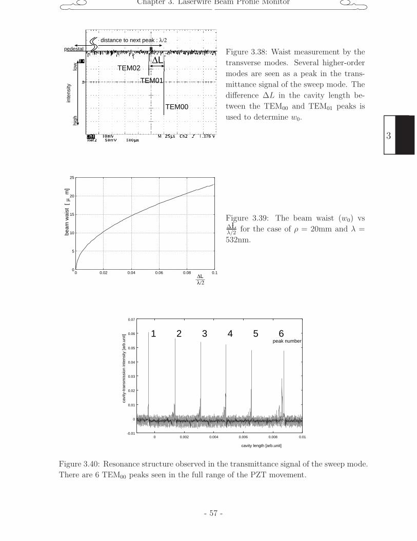
Chapter 3. Laserwire Beam Profile Monitor
pedestal
inte
nsity
high
low
TEM00
TEM01
∆L
distance to next peak : λ/2
TEM02
Figure 3.38: Waist measurement by the
transverse modes. Several higher-order
modes are seen as a peak in the trans-
mittance signal of the sweep mode. The
difference ∆L in the cavity length be-
tween the TEM00 and TEM01 peaks is
used to determine w0.
0
5
10
15
20
25
0 0.02 0.04 0.06 0.08 0.1
beam
wai
st [
m]
µ
λ/2∆L
Figure 3.39: The beam waist (w0) vs∆Lλ/2
for the case of ρ = 20mm and λ =
532nm.
-0.01
0
0.01
0.02
0.03
0.04
0.05
0.06
0.07
0 0.002 0.004 0.006 0.008 0.01
cavi
ty-t
rans
mis
sion
inte
nsity
[arb
.uni
t]
cavity length [arb.unit]
1 2 3 4 5 6peak number
Figure 3.40: Resonance structure observed in the transmittance signal of the sweep mode.
There are 6 TEM00 peaks seen in the full range of the PZT movement.
- 57 -
3
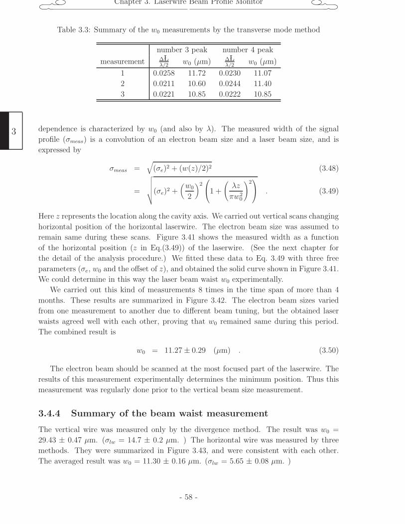
Chapter 3. Laserwire Beam Profile Monitor
Table 3.3: Summary of the w0 measurements by the transverse mode method
number 3 peak number 4 peak
measurement ∆Lλ/2
w0 (µm) ∆Lλ/2
w0 (µm)
1 0.0258 11.72 0.0230 11.07
2 0.0211 10.60 0.0244 11.40
3 0.0221 10.85 0.0222 10.85
dependence is characterized by w0 (and also by λ). The measured width of the signal
profile (σmeas) is a convolution of an electron beam size and a laser beam size, and is
expressed by
σmeas =√
(σe)2 + (w(z)/2)2 (3.48)
=
√√√√√(σe)2 +(w0
2
)2⎛⎝1 +
(λz
πw20
)2⎞⎠ . (3.49)
Here z represents the location along the cavity axis. We carried out vertical scans changing
horizontal position of the horizontal laserwire. The electron beam size was assumed to
remain same during these scans. Figure 3.41 shows the measured width as a function
of the horizontal position (z in Eq.(3.49)) of the laserwire. (See the next chapter for
the detail of the analysis procedure.) We fitted these data to Eq. 3.49 with three free
parameters (σe, w0 and the offset of z), and obtained the solid curve shown in Figure 3.41.
We could determine in this way the laser beam waist w0 experimentally.
We carried out this kind of measurements 8 times in the time span of more than 4
months. These results are summarized in Figure 3.42. The electron beam sizes varied
from one measurement to another due to different beam tuning, but the obtained laser
waists agreed well with each other, proving that w0 remained same during this period.
The combined result is
w0 = 11.27 ± 0.29 (µm) . (3.50)
The electron beam should be scanned at the most focused part of the laserwire. The
results of this measurement experimentally determines the minimum position. Thus this
measurement was regularly done prior to the vertical beam size measurement.
3.4.4 Summary of the beam waist measurement
The vertical wire was measured only by the divergence method. The result was w0 =
29.43 ± 0.47 µm. (σlw = 14.7 ± 0.2 µm. ) The horizontal wire was measured by three
methods. They were summarized in Figure 3.43, and were consistent with each other.
The averaged result was w0 = 11.30 ± 0.16 µm. (σlw = 5.65 ± 0.08 µm. )
3
- 58 -
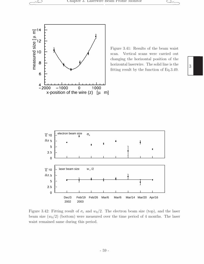
Chapter 3. Laserwire Beam Profile Monitor
mea
sure
d si
ze [
m
]µ
x-position of the wire (z) [ m]µ
Figure 3.41: Results of the beam waist
scan. Vertical scans were carried out
changing the horizontal position of the
horizontal laserwire. The solid line is the
fitting result by the function of Eq.3.49.
electron beam size
laser beam size
µ [
m]
µ [
m]
Dec/3 Feb/19 Feb/26 Mar/6 Mar/6 Mar/14 Mar/20 Apr/162002 2003
w /20
σe
Figure 3.42: Fitting result of σe and w0/2. The electron beam size (top), and the laser
beam size (w0/2) (bottom) were measured over the time period of 4 months. The laser
waist remained same during this period.
- 59 -
3
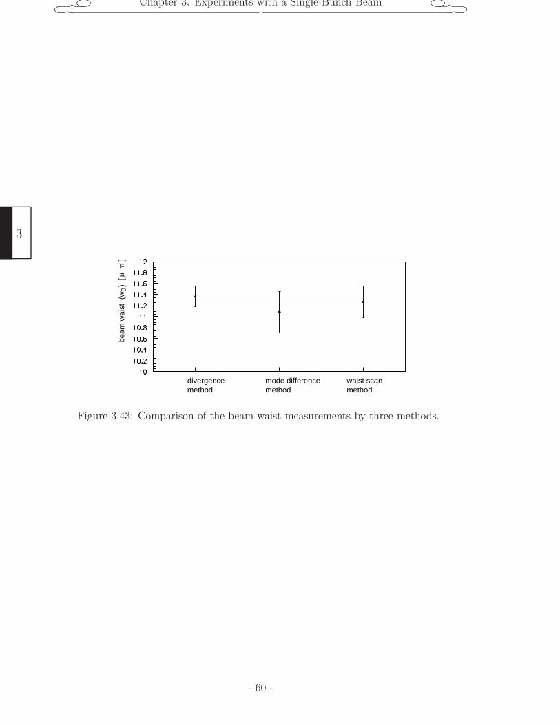
Chapter 3. Experiments with a Single-Bunch Beam
divergencemethod
mode differencemethod
waist scanmethod
beam
wai
st (
w )
[
m ]
µ0
Figure 3.43: Comparison of the beam waist measurements by three methods.
3
- 60 -
Chapter 4. Experiments with a Single-Bunch Beam
Chapter 4
Experiments with a Single-Bunch
Beam
We performed a series of emittance measurements with a single bunch beam stored in
the damping ring over the time period of four months from February 2003 to May 2003
([33]). Although the goal of the ATF damping ring is to confirm realization of the target
emittance with a multi-bunch beam, verification with a single-bunch beam is the first
important step to be done. Also a single bunch beam is suitable for studying basic
beam dynamics such as intra-beam scattering, which are not related to the coupled-bunch
motion.
The main purposes of this experiment were :
1. Verification of a stable production of a low emittance beam satisfying the require-
ments of the linear colliders.
2. Observation of possible emittance dilution which depends on the beam intensity
under various beam conditions, and understanding the mechanisms of the emittance
growth.
4.1 Introduction
4.1.1 Emittance measurements prior to this experiment
First, we give a short review of the results of emittance studies at the moment we started
this experiment ([34]).
As the first step after the ATF commissioning, an extracted beam was examined by
the solid-wire scanner system ([35]). The production of a small emittance, 1.37 ± 0.03
nm·rad, in the horizontal plane at the bunch intensity of 3-5×10⁹ electrons was confirmed.
This should be compared with the expected value of 1.27-1.34 nm·rad which included the
effect of intra-beam scattering to the designed natural emittance of 1.07 nm·rad. The
result was a good verification of the ring design.
Then the next step was to measure the vertical emittance. The target value for the
vertical emittance was 1% of the horizontal one. The smallness of the vertical emittance
- 61 -
4
Chapter 4. Experiments with a Single-Bunch Beam
posed a number of difficulties for the measurement system. In the extraction line, it
was not easy to stabilize the beam orbit within a fraction of the vertical beam size. It
was also not straightforward to estimate actual emittances from measured values. This
was because, in the diagnostic section of the extraction line, even a small amount of the
residual dispersion could mimic an apparent (false) vertical beam size. A technique for
the precision measurement of the dispersion effect and its correction had to be developed
for an accurate measurement. Another difficulty was the x-y coupling. Some unknown
coupling source could give a small tilt in the transverse beam profile. Due to the high
aspect ratio of the beam profile, the vertical size could easily be contaminated by the much
bigger horizontal sizes. We struggled to find out the hidden coupling sources and/or to
correct them by introducing additional skew magnets.
Systematic studies of the emittance in the extraction line were continued from April
2000 to June 2001 ([36],[37]). From the studies, the vertical emittance was found to be
15 pm·rad for low intensity and to grow to 23 pm·rad at the beam intensity of 8 × 10⁹
electrons per bunch. This outcome gave rise to puzzles as well as interests ([38]); the
intensity dependence of the vertical emittance was surprisingly strong, and could not
be reproduced by the standard calculation involving the intra-beam scattering, which
explained well the horizontal intensity dependence. Various scenarios were considered
to explain the observation; for example, possibilities to require a modification in the
intra-beam scattering model, and/or existence of other intensity dependent effects in the
vertical plane. However, considering the measurement difficulties mentioned above, it was
concluded that there might be still unknown measurement errors, and they were the most
likely source of the disagreement. At the same time, the importance of the measurement
in the ring itself was stressed.
As for the measurement in the ring, we had been developing the SR interferometer
monitor since the beginning of the ring operation. This monitor worked well for a large
beam size. However, its practical resolution limit was found to be around 10 µm. The
system was not understood well enough for such a small vertical size of our interest.
The commissioning of the laserwire monitor started in May 2000. The first vertical
emittance measurement was carried out in December 2000 [39], and it resulted (11.8±0.8)
pm·rad as the average of all the data points. No clear dependence on the beam intensity
was observed within the measurement errors dominated by the statistical fluctuation.
The results in the extraction line (by the solid-wire scanner) and in the ring (by the
laserwire and SR monitor) at this moment are plotted in Figure 4.1.
4.1.2 Improvements to the ATF damping ring
To settle the issue on the current dependence of the vertical emittance, we focused our
efforts to accurate measurements in the ring: upgrade of the laserwire. At the same
time, various efforts were made to reduce the emittance further. We first describe several
essential improvements to the ATF damping ring itself. They are as follows:
1. The read-out circuits for the beam position monitors (BPMs) in the damping ring
were replaced by a new type. Their position resolution was, thereby, improved from
4
- 62 -
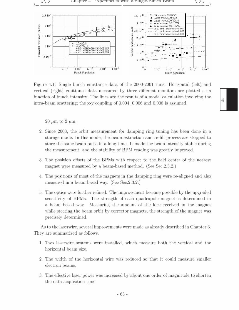
Chapter 4. Experiments with a Single-Bunch Beam
Figure 4.1: Single bunch emittance data of the 2000-2001 runs: Horizontal (left) and
vertical (right) emittance data measured by three different monitors are plotted as a
function of bunch intensity. The lines are the results of a model calculation involving the
intra-beam scattering; the x-y coupling of 0.004, 0.006 and 0.008 is assumed.
20 µm to 2 µm.
2. Since 2003, the orbit measurement for damping ring tuning has been done in a
storage mode. In this mode, the beam extraction and re-fill process are stopped to
store the same beam pulse in a long time. It made the beam intensity stable during
the measurement, and the stability of BPM reading was greatly improved.
3. The position offsets of the BPMs with respect to the field center of the nearest
magnet were measured by a beam-based method. (See Sec.2.3.2.)
4. The positions of most of the magnets in the damping ring were re-aligned and also
measured in a beam based way. (See Sec.2.3.2.)
5. The optics were further refined. The improvement became possible by the upgraded
sensitivity of BPMs. The strength of each quadrupole magnet is determined in
a beam based way. Measuring the amount of the kick received in the magnet
while steering the beam orbit by corrector magnets, the strength of the magnet was
precisely determined.
As to the laserwire, several improvements were made as already described in Chapter 3.
They are summarized as follows.
1. Two laserwire systems were installed, which measure both the vertical and the
horizontal beam size.
2. The width of the horizontal wire was reduced so that it could measure smaller
electron beams.
3. The effective laser power was increased by about one order of magnitude to shorten
the data acquisition time.
- 63 -
4
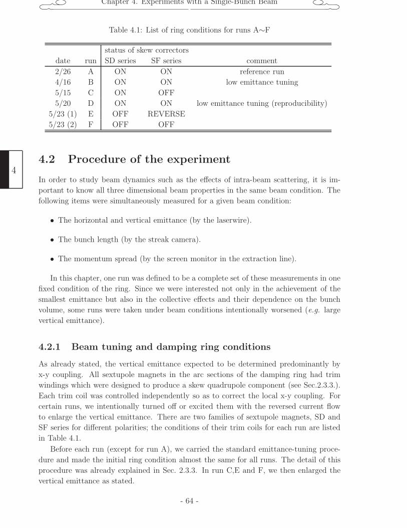
Chapter 4. Experiments with a Single-Bunch Beam
Table 4.1: List of ring conditions for runs A∼F
status of skew correctors
date run SD series SF series comment
2/26 A ON ON reference run
4/16 B ON ON low emittance tuning
5/15 C ON OFF
5/20 D ON ON low emittance tuning (reproducibility)
5/23 (1) E OFF REVERSE
5/23 (2) F OFF OFF
4.2 Procedure of the experiment
In order to study beam dynamics such as the effects of intra-beam scattering, it is im-
portant to know all three dimensional beam properties in the same beam condition. The
following items were simultaneously measured for a given beam condition:
• The horizontal and vertical emittance (by the laserwire).
• The bunch length (by the streak camera).
• The momentum spread (by the screen monitor in the extraction line).
In this chapter, one run was defined to be a complete set of these measurements in one
fixed condition of the ring. Since we were interested not only in the achievement of the
smallest emittance but also in the collective effects and their dependence on the bunch
volume, some runs were taken under beam conditions intentionally worsened (e.g. large
vertical emittance).
4.2.1 Beam tuning and damping ring conditions
As already stated, the vertical emittance expected to be determined predominantly by
x-y coupling. All sextupole magnets in the arc sections of the damping ring had trim
windings which were designed to produce a skew quadrupole component (see Sec.2.3.3.).
Each trim coil was controlled independently so as to correct the local x-y coupling. For
certain runs, we intentionally turned off or excited them with the reversed current flow
to enlarge the vertical emittance. There are two families of sextupole magnets, SD and
SF series for different polarities; the conditions of their trim coils for each run are listed
in Table 4.1.
Before each run (except for run A), we carried the standard emittance-tuning proce-
dure and made the initial ring condition almost the same for all runs. The detail of this
procedure was already explained in Sec. 2.3.3. In run C,E and F, we then enlarged the
vertical emittance as stated.
4
- 64 -
Chapter 4. Experiments with a Single-Bunch Beam
4.2.2 Measurements of transverse beam profiles
One of the main goals of the study is to clearify the intensity dependence of the emittances.
We thus made the measurements up to the maximum possible intensity. Actually, there
existed typically 9 scans in a run with each scan being for a certain intensity region.
Although the scanning and data acquisition were automated for the most part, beam
injection into the damping ring and intensity control had to be done manually.
Data taking
As we stressed, the electron beam intensity was one of the most important parameters.
For each scan, we defined the intensity to be measured (we call it intended intensity
region). To realize it, the emission of the electron gun was tuned, and the injected beam
intensity was made to agree with the maximum of the intended intensity region. After
the beam was stored in the ring, the scanning process was started. One scan was defined
to be one complete round trip measuring an entire electron profile. Typical data taking
procedures are shown in Figure 4.2∼4.3; the beam current, the position of the laserwire
and the measured signal rate are plotted as a function of the data-acquisition time. During
the measurement, the electron beam current decreased according to its life time. When
the current reached the minimum of the intended intensity region, the data taking was
manually paused to re-fill an electron beam and then it was resumed. Thus data of one
scan contained several fills, especially in the data of a high intensity region. Since the
damping time of the ring was around 20 msec, the stored beam immediately reached the
equilibrium. We assumed that the multiple fills had no effect on our measurement. It took
about 6 minutes for a vertical scan, and 15 minutes for horizontal. The beam-intensity
region, required number of fills and total number of data points for each scan are listed
in Table 4.2∼4.7. The average beam current during the scan and its rms variation are
also listed. We used these values as the average and its interval of the intended intensity
region.
Fitting of the signal profile
The first step of the analysis is to plot the signal profile. The current-normalized signal
rate (Hz/mA) was calculated, and was plotted as a function of the laserwire position.
Figure 4.4 and 4.5 are examples of such measurements for vertical and horizontal direc-
tions. We fitted these data points by a Gauss function with three free parameters ( peak
height, position and width ). We defined the width of the fitted Gauss function as the
measured peak width (σmeas). The resultant σmeas values are listed in the last column
but one in Table 4.2∼4.7. The chi-square (χ2) per degree of freedom (ν) of the fit is also
listed. The value of χ2/ν larger than unity indicates existence of some systematic effects.
It has been observed that there exists a slow beam orbit drift in a few 100 seconds time
scale. Since the vertical beam size was as small as 5 µm, even orbit drift of 1 µm order (
much less than the measurement accuracy of the BPMs ) could affect the measurement.
We suspect a temperature change in some component of the ring caused this drift. In any
case, to include the effect of the systematic effects, we took a conservative way. Namely,
- 65 -
4
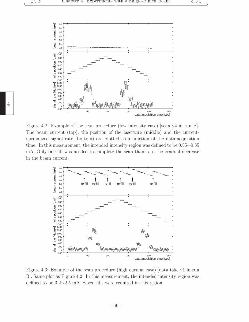
Chapter 4. Experiments with a Single-Bunch Beam
0.0
0.5
1.0
1.5
2.0
2.5
3.0
3.5
-700
-680
-660
-640
-620
-600
-580
-560
-2000
200400600800
100012001400
0 50 100 150 200 250
beam
cur
rent
[mA
]w
ire p
ositi
on [
m]
µsi
gnal
rat
e [H
z/m
A]
data acquisition time [sec]
Figure 4.2: Example of the scan procedure (low intensity case) [scan y4 in run B].
The beam current (top), the position of the laserwire (middle) and the current-
normalized signal rate (bottom) are plotted as a function of the data-acquisition
time. In this measurement, the intended intensity region was defined to be 0.55∼0.35
mA. Only one fill was needed to complete the scan thanks to the gradual decrease
in the beam current.
0.0
0.5
1.0
1.5
2.0
2.5
3.0
3.5
-700
-680
-660
-640
-620
-600
-580
-560
-2000
200400600800
100012001400
0 50 100 150 200 250
beam
cur
rent
[mA
]w
ire p
ositi
on [
m]
µsi
gnal
rat
e [H
z/m
A]
data acquisition time [sec]
re-fill re-fill re-fill re-fill re-fill re-fill
Figure 4.3: Example of the scan procedure (high current case) [data take y1 in run
B]. Same plot as Figure 4.2. In this measurement, the intended intensity region was
defined to be 3.2∼2.5 mA. Seven fills were required in this region.
4
- 66 -
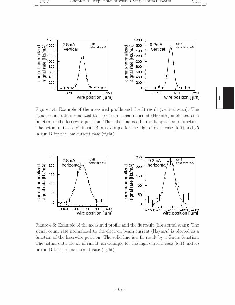
Chapter 4. Experiments with a Single-Bunch Beam
curr
ent-
norm
aliz
edsi
gnal
rat
e [H
z/m
A]
curr
ent-
norm
aliz
edsi
gnal
rat
e [H
z/m
A]
wire position [ m]µ wire position [ m]µ
2.8mA 0.2mAvertical vertical
runBdata take y-1
runBdata take y-5
Figure 4.4: Example of the measured profile and the fit result (vertical scan): The
signal count rate normalized to the electron beam current (Hz/mA) is plotted as a
function of the laserwire position. The solid line is a fit result by a Gauss function.
The actual data are y1 in run B, an example for the high current case (left) and y5
in run B for the low current case (right).
curr
ent-
norm
aliz
edsi
gnal
rat
e [H
z/m
A]
curr
ent-
norm
aliz
edsi
gnal
rat
e [H
z/m
A]
wire position [ m]µ wire position [ m]µ
2.8mA 0.2mAhorizontal horizontal
runBdata take x-1
runBdata take x-5
Figure 4.5: Example of the measured profile and the fit result (horizontal scan): The
signal count rate normalized to the electron beam current (Hz/mA) is plotted as a
function of the laserwire position. The solid line is a fit result by a Gauss function.
The actual data are x1 in run B, an example for the high current case (left) and x5
in run B for the low current case (right).
- 67 -
4
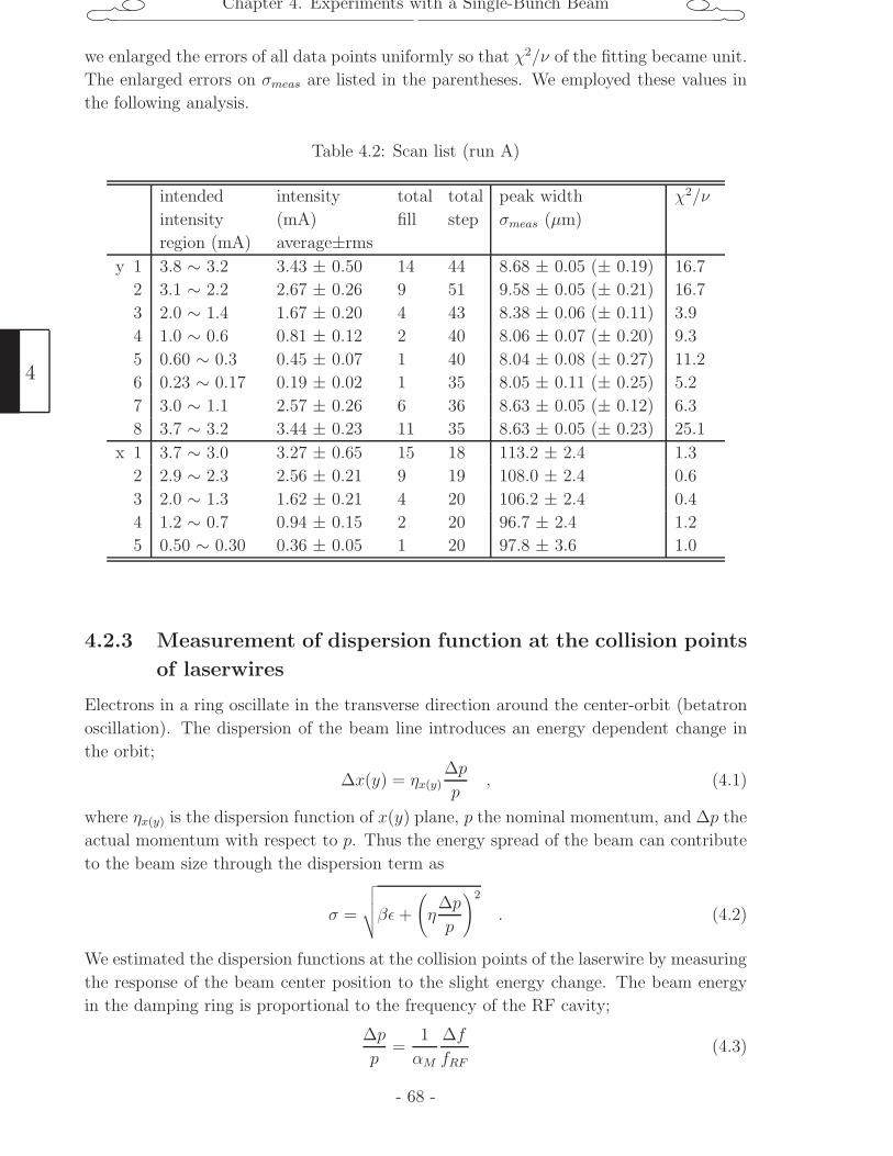
Chapter 4. Experiments with a Single-Bunch Beam
we enlarged the errors of all data points uniformly so that χ2/ν of the fitting became unit.
The enlarged errors on σmeas are listed in the parentheses. We employed these values in
the following analysis.
Table 4.2: Scan list (run A)
intended
intensity
region (mA)
intensity
(mA)
average±rms
total
fill
total
step
peak width
σmeas (µm)
χ2/ν
y 1 3.8 ∼ 3.2 3.43 ± 0.50 14 44 8.68 ± 0.05 (± 0.19) 16.7
2 3.1 ∼ 2.2 2.67 ± 0.26 9 51 9.58 ± 0.05 (± 0.21) 16.7
3 2.0 ∼ 1.4 1.67 ± 0.20 4 43 8.38 ± 0.06 (± 0.11) 3.9
4 1.0 ∼ 0.6 0.81 ± 0.12 2 40 8.06 ± 0.07 (± 0.20) 9.3
5 0.60 ∼ 0.3 0.45 ± 0.07 1 40 8.04 ± 0.08 (± 0.27) 11.2
6 0.23 ∼ 0.17 0.19 ± 0.02 1 35 8.05 ± 0.11 (± 0.25) 5.2
7 3.0 ∼ 1.1 2.57 ± 0.26 6 36 8.63 ± 0.05 (± 0.12) 6.3
8 3.7 ∼ 3.2 3.44 ± 0.23 11 35 8.63 ± 0.05 (± 0.23) 25.1
x 1 3.7 ∼ 3.0 3.27 ± 0.65 15 18 113.2 ± 2.4 1.3
2 2.9 ∼ 2.3 2.56 ± 0.21 9 19 108.0 ± 2.4 0.6
3 2.0 ∼ 1.3 1.62 ± 0.21 4 20 106.2 ± 2.4 0.4
4 1.2 ∼ 0.7 0.94 ± 0.15 2 20 96.7 ± 2.4 1.2
5 0.50 ∼ 0.30 0.36 ± 0.05 1 20 97.8 ± 3.6 1.0
4.2.3 Measurement of dispersion function at the collision points
of laserwires
Electrons in a ring oscillate in the transverse direction around the center-orbit (betatron
oscillation). The dispersion of the beam line introduces an energy dependent change in
the orbit;
∆x(y) = ηx(y)∆p
p, (4.1)
where ηx(y) is the dispersion function of x(y) plane, p the nominal momentum, and ∆p the
actual momentum with respect to p. Thus the energy spread of the beam can contribute
to the beam size through the dispersion term as
σ =
√√√√βε+
(η
∆p
p
)2
. (4.2)
We estimated the dispersion functions at the collision points of the laserwire by measuring
the response of the beam center position to the slight energy change. The beam energy
in the damping ring is proportional to the frequency of the RF cavity;
∆p
p=
1
αM
∆f
fRF
(4.3)
4
- 68 -
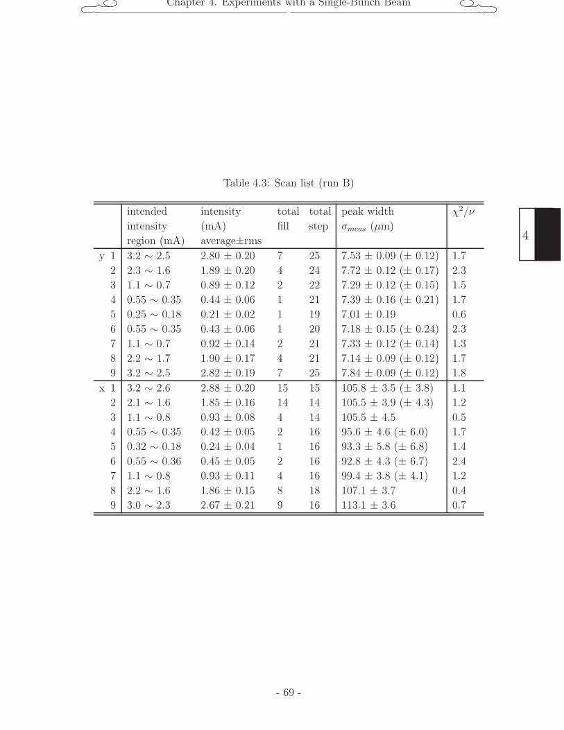
Chapter 4. Experiments with a Single-Bunch Beam
Table 4.3: Scan list (run B)
intended
intensity
region (mA)
intensity
(mA)
average±rms
total
fill
total
step
peak width
σmeas (µm)
χ2/ν
y 1 3.2 ∼ 2.5 2.80 ± 0.20 7 25 7.53 ± 0.09 (± 0.12) 1.7
2 2.3 ∼ 1.6 1.89 ± 0.20 4 24 7.72 ± 0.12 (± 0.17) 2.3
3 1.1 ∼ 0.7 0.89 ± 0.12 2 22 7.29 ± 0.12 (± 0.15) 1.5
4 0.55 ∼ 0.35 0.44 ± 0.06 1 21 7.39 ± 0.16 (± 0.21) 1.7
5 0.25 ∼ 0.18 0.21 ± 0.02 1 19 7.01 ± 0.19 0.6
6 0.55 ∼ 0.35 0.43 ± 0.06 1 20 7.18 ± 0.15 (± 0.24) 2.3
7 1.1 ∼ 0.7 0.92 ± 0.14 2 21 7.33 ± 0.12 (± 0.14) 1.3
8 2.2 ∼ 1.7 1.90 ± 0.17 4 21 7.14 ± 0.09 (± 0.12) 1.7
9 3.2 ∼ 2.5 2.82 ± 0.19 7 25 7.84 ± 0.09 (± 0.12) 1.8
x 1 3.2 ∼ 2.6 2.88 ± 0.20 15 15 105.8 ± 3.5 (± 3.8) 1.1
2 2.1 ∼ 1.6 1.85 ± 0.16 14 14 105.5 ± 3.9 (± 4.3) 1.2
3 1.1 ∼ 0.8 0.93 ± 0.08 4 14 105.5 ± 4.5 0.5
4 0.55 ∼ 0.35 0.42 ± 0.05 2 16 95.6 ± 4.6 (± 6.0) 1.7
5 0.32 ∼ 0.18 0.24 ± 0.04 1 16 93.3 ± 5.8 (± 6.8) 1.4
6 0.55 ∼ 0.36 0.45 ± 0.05 2 16 92.8 ± 4.3 (± 6.7) 2.4
7 1.1 ∼ 0.8 0.93 ± 0.11 4 16 99.4 ± 3.8 (± 4.1) 1.2
8 2.2 ∼ 1.6 1.86 ± 0.15 8 18 107.1 ± 3.7 0.4
9 3.0 ∼ 2.3 2.67 ± 0.21 9 16 113.1 ± 3.6 0.7
- 69 -
4
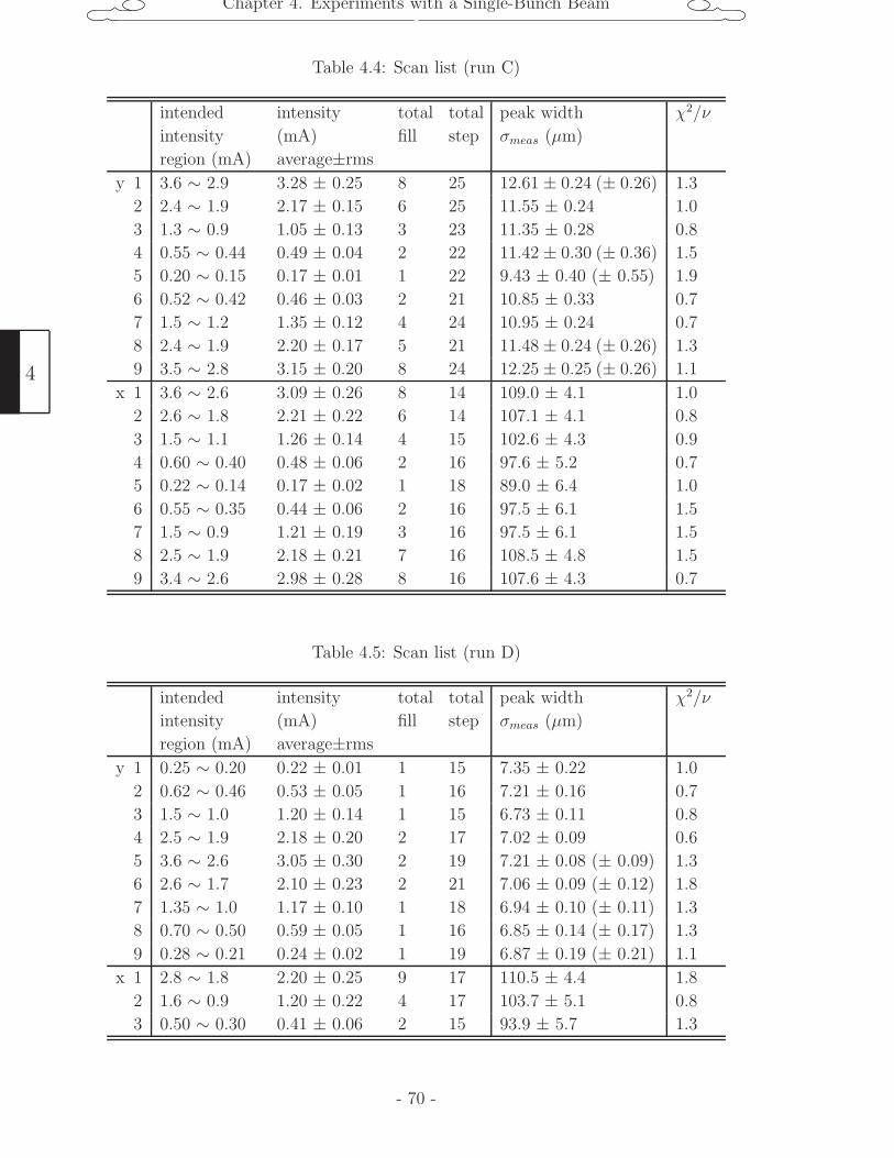
Chapter 4. Experiments with a Single-Bunch Beam
Table 4.4: Scan list (run C)
intended
intensity
region (mA)
intensity
(mA)
average±rms
total
fill
total
step
peak width
σmeas (µm)
χ2/ν
y 1 3.6 ∼ 2.9 3.28 ± 0.25 8 25 12.61 ± 0.24 (± 0.26) 1.3
2 2.4 ∼ 1.9 2.17 ± 0.15 6 25 11.55 ± 0.24 1.0
3 1.3 ∼ 0.9 1.05 ± 0.13 3 23 11.35 ± 0.28 0.8
4 0.55 ∼ 0.44 0.49 ± 0.04 2 22 11.42 ± 0.30 (± 0.36) 1.5
5 0.20 ∼ 0.15 0.17 ± 0.01 1 22 9.43 ± 0.40 (± 0.55) 1.9
6 0.52 ∼ 0.42 0.46 ± 0.03 2 21 10.85 ± 0.33 0.7
7 1.5 ∼ 1.2 1.35 ± 0.12 4 24 10.95 ± 0.24 0.7
8 2.4 ∼ 1.9 2.20 ± 0.17 5 21 11.48 ± 0.24 (± 0.26) 1.3
9 3.5 ∼ 2.8 3.15 ± 0.20 8 24 12.25 ± 0.25 (± 0.26) 1.1
x 1 3.6 ∼ 2.6 3.09 ± 0.26 8 14 109.0 ± 4.1 1.0
2 2.6 ∼ 1.8 2.21 ± 0.22 6 14 107.1 ± 4.1 0.8
3 1.5 ∼ 1.1 1.26 ± 0.14 4 15 102.6 ± 4.3 0.9
4 0.60 ∼ 0.40 0.48 ± 0.06 2 16 97.6 ± 5.2 0.7
5 0.22 ∼ 0.14 0.17 ± 0.02 1 18 89.0 ± 6.4 1.0
6 0.55 ∼ 0.35 0.44 ± 0.06 2 16 97.5 ± 6.1 1.5
7 1.5 ∼ 0.9 1.21 ± 0.19 3 16 97.5 ± 6.1 1.5
8 2.5 ∼ 1.9 2.18 ± 0.21 7 16 108.5 ± 4.8 1.5
9 3.4 ∼ 2.6 2.98 ± 0.28 8 16 107.6 ± 4.3 0.7
Table 4.5: Scan list (run D)
intended
intensity
region (mA)
intensity
(mA)
average±rms
total
fill
total
step
peak width
σmeas (µm)
χ2/ν
y 1 0.25 ∼ 0.20 0.22 ± 0.01 1 15 7.35 ± 0.22 1.0
2 0.62 ∼ 0.46 0.53 ± 0.05 1 16 7.21 ± 0.16 0.7
3 1.5 ∼ 1.0 1.20 ± 0.14 1 15 6.73 ± 0.11 0.8
4 2.5 ∼ 1.9 2.18 ± 0.20 2 17 7.02 ± 0.09 0.6
5 3.6 ∼ 2.6 3.05 ± 0.30 2 19 7.21 ± 0.08 (± 0.09) 1.3
6 2.6 ∼ 1.7 2.10 ± 0.23 2 21 7.06 ± 0.09 (± 0.12) 1.8
7 1.35 ∼ 1.0 1.17 ± 0.10 1 18 6.94 ± 0.10 (± 0.11) 1.3
8 0.70 ∼ 0.50 0.59 ± 0.05 1 16 6.85 ± 0.14 (± 0.17) 1.3
9 0.28 ∼ 0.21 0.24 ± 0.02 1 19 6.87 ± 0.19 (± 0.21) 1.1
x 1 2.8 ∼ 1.8 2.20 ± 0.25 9 17 110.5 ± 4.4 1.8
2 1.6 ∼ 0.9 1.20 ± 0.22 4 17 103.7 ± 5.1 0.8
3 0.50 ∼ 0.30 0.41 ± 0.06 2 15 93.9 ± 5.7 1.3
4
- 70 -
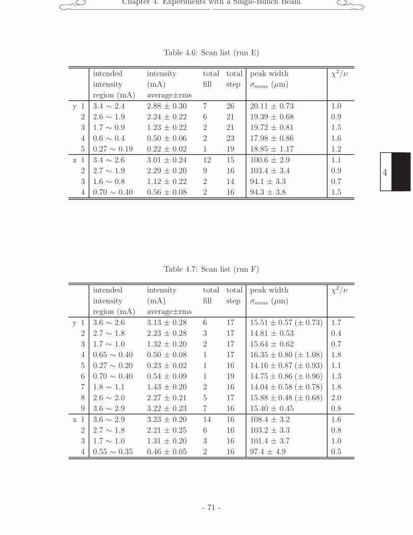
Chapter 4. Experiments with a Single-Bunch Beam
Table 4.6: Scan list (run E)
intended
intensity
region (mA)
intensity
(mA)
average±rms
total
fill
total
step
peak width
σmeas (µm)
χ2/ν
y 1 3.4 ∼ 2.4 2.88 ± 0.30 7 26 20.11 ± 0.73 1.0
2 2.6 ∼ 1.9 2.24 ± 0.22 6 21 19.39 ± 0.68 0.9
3 1.7 ∼ 0.9 1.23 ± 0.22 2 21 19.72 ± 0.81 1.5
4 0.6 ∼ 0.4 0.50 ± 0.06 2 23 17.98 ± 0.86 1.6
5 0.27 ∼ 0.19 0.22 ± 0.02 1 19 18.85 ± 1.17 1.2
x 1 3.4 ∼ 2.6 3.01 ± 0.24 12 15 100.6 ± 2.9 1.1
2 2.7 ∼ 1.9 2.29 ± 0.20 9 16 103.4 ± 3.4 0.9
3 1.6 ∼ 0.8 1.12 ± 0.22 2 14 94.1 ± 3.3 0.7
4 0.70 ∼ 0.40 0.56 ± 0.08 2 16 94.3 ± 3.8 1.5
Table 4.7: Scan list (run F)
intended
intensity
region (mA)
intensity
(mA)
average±rms
total
fill
total
step
peak width
σmeas (µm)
χ2/ν
y 1 3.6 ∼ 2.6 3.13 ± 0.28 6 17 15.51 ± 0.57 (± 0.73) 1.7
2 2.7 ∼ 1.8 2.23 ± 0.28 3 17 14.81 ± 0.53 0.4
3 1.7 ∼ 1.0 1.32 ± 0.20 2 17 15.64 ± 0.62 0.7
4 0.65 ∼ 0.40 0.50 ± 0.08 1 17 16.35 ± 0.80 (± 1.08) 1.8
5 0.27 ∼ 0.20 0.23 ± 0.02 1 16 14.16 ± 0.87 (± 0.93) 1.1
6 0.70 ∼ 0.40 0.54 ± 0.09 1 19 14.75 ± 0.86 (± 0.96) 1.3
7 1.8 ∼ 1.1 1.43 ± 0.20 2 16 14.04 ± 0.58 (± 0.78) 1.8
8 2.6 ∼ 2.0 2.27 ± 0.21 5 17 15.88 ± 0.48 (± 0.68) 2.0
9 3.6 ∼ 2.9 3.22 ± 0.23 7 16 15.40 ± 0.45 0.8
x 1 3.6 ∼ 2.9 3.23 ± 0.20 14 16 108.4 ± 3.2 1.6
2 2.7 ∼ 1.8 2.21 ± 0.25 6 16 103.2 ± 3.3 0.8
3 1.7 ∼ 1.0 1.31 ± 0.20 3 16 101.4 ± 3.7 1.0
4 0.55 ∼ 0.35 0.46 ± 0.05 2 16 97.4 ± 4.9 0.5
- 71 -
4
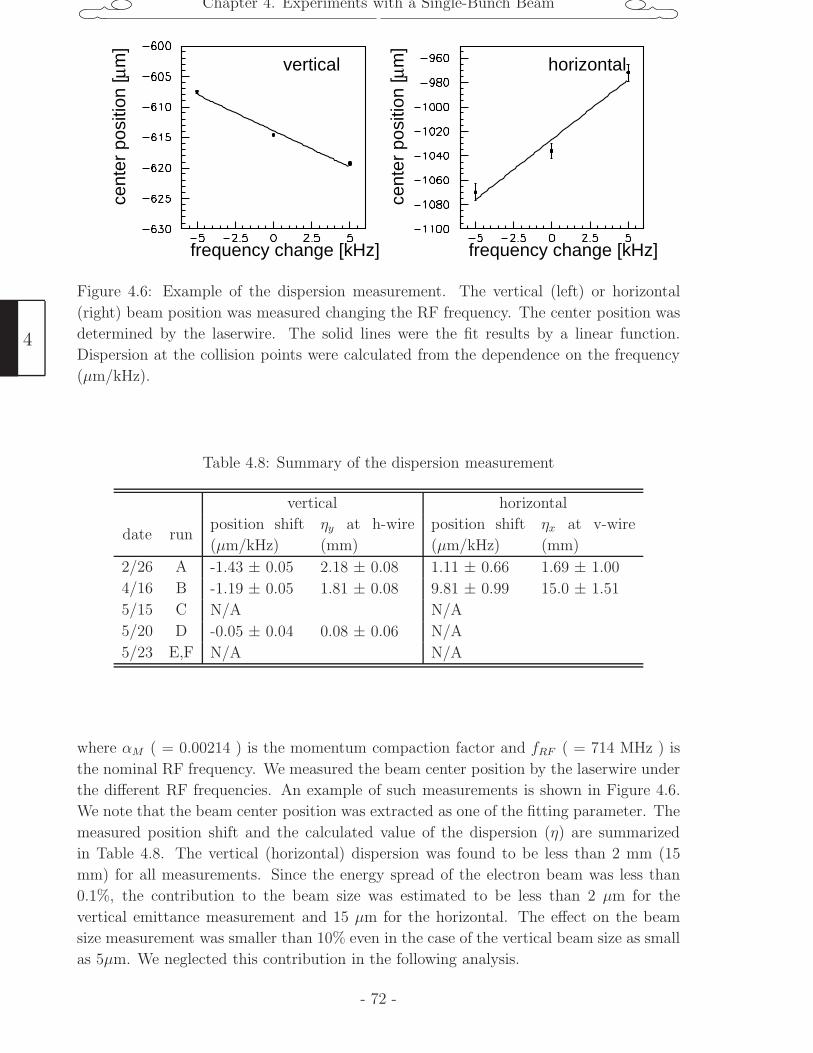
Chapter 4. Experiments with a Single-Bunch Beam
cent
er p
ositi
on [
m]
µ
frequency change [kHz] frequency change [kHz]
cent
er p
ositi
on [
m]
µvertical horizontal
Figure 4.6: Example of the dispersion measurement. The vertical (left) or horizontal
(right) beam position was measured changing the RF frequency. The center position was
determined by the laserwire. The solid lines were the fit results by a linear function.
Dispersion at the collision points were calculated from the dependence on the frequency
(µm/kHz).
Table 4.8: Summary of the dispersion measurement
vertical horizontal
date runposition shift
(µm/kHz)
ηy at h-wire
(mm)
position shift
(µm/kHz)
ηx at v-wire
(mm)
2/26 A -1.43 ± 0.05 2.18 ± 0.08 1.11 ± 0.66 1.69 ± 1.00
4/16 B -1.19 ± 0.05 1.81 ± 0.08 9.81 ± 0.99 15.0 ± 1.51
5/15 C N/A N/A
5/20 D -0.05 ± 0.04 0.08 ± 0.06 N/A
5/23 E,F N/A N/A
where αM ( = 0.00214 ) is the momentum compaction factor and fRF ( = 714 MHz ) is
the nominal RF frequency. We measured the beam center position by the laserwire under
the different RF frequencies. An example of such measurements is shown in Figure 4.6.
We note that the beam center position was extracted as one of the fitting parameter. The
measured position shift and the calculated value of the dispersion (η) are summarized
in Table 4.8. The vertical (horizontal) dispersion was found to be less than 2 mm (15
mm) for all measurements. Since the energy spread of the electron beam was less than
0.1%, the contribution to the beam size was estimated to be less than 2 µm for the
vertical emittance measurement and 15 µm for the horizontal. The effect on the beam
size measurement was smaller than 10% even in the case of the vertical beam size as small
as 5µm. We neglected this contribution in the following analysis.
4
- 72 -
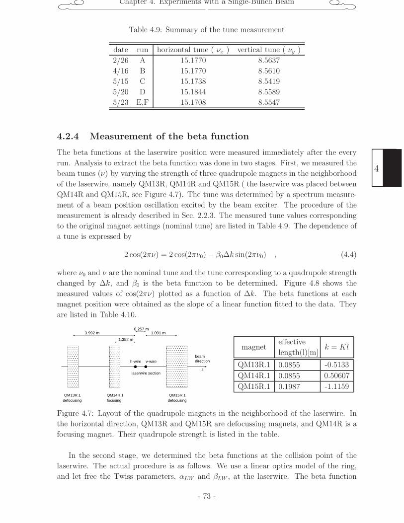
Chapter 4. Experiments with a Single-Bunch Beam
Table 4.9: Summary of the tune measurement
date run horizontal tune ( νx ) vertical tune ( νy )
2/26 A 15.1770 8.5637
4/16 B 15.1770 8.5610
5/15 C 15.1738 8.5419
5/20 D 15.1844 8.5589
5/23 E,F 15.1708 8.5547
4.2.4 Measurement of the beta function
The beta functions at the laserwire position were measured immediately after the every
run. Analysis to extract the beta function was done in two stages. First, we measured the
beam tunes (ν) by varying the strength of three quadrupole magnets in the neighborhood
of the laserwire, namely QM13R, QM14R and QM15R ( the laserwire was placed between
QM14R and QM15R, see Figure 4.7). The tune was determined by a spectrum measure-
ment of a beam position oscillation excited by the beam exciter. The procedure of the
measurement is already described in Sec. 2.2.3. The measured tune values corresponding
to the original magnet settings (nominal tune) are listed in Table 4.9. The dependence of
a tune is expressed by
2 cos(2πν) = 2 cos(2πν0) − β0∆k sin(2πν0) , (4.4)
where ν0 and ν are the nominal tune and the tune corresponding to a quadrupole strength
changed by ∆k, and β0 is the beta function to be determined. Figure 4.8 shows the
measured values of cos(2πν) plotted as a function of ∆k. The beta functions at each
magnet position were obtained as the slope of a linear function fitted to the data. They
are listed in Table 4.10.
QM13R.1 QM14R.1 QM15R.1
3.992 m 1.091 m0.257 m
1.352 m
h-wire v-wire
defocusing focusing defocusing
beam direction
slaserwire section
magneteffective
length(l)[m]k = Kl
QM13R.1 0.0855 -0.5133
QM14R.1 0.0855 0.50607
QM15R.1 0.1987 -1.1159
Figure 4.7: Layout of the quadrupole magnets in the neighborhood of the laserwire. In
the horizontal direction, QM13R and QM15R are defocussing magnets, and QM14R is a
focusing magnet. Their quadrupole strength is listed in the table.
In the second stage, we determined the beta functions at the collision point of the
laserwire. The actual procedure is as follows. We use a linear optics model of the ring,
and let free the Twiss parameters, αLW and βLW , at the laserwire. The beta function
- 73 -
4
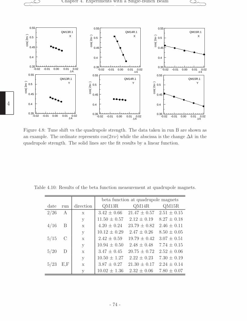
Chapter 4. Experiments with a Single-Bunch Beam
QM13R.1
X
QM14R.1
X
QM15R.1
X
QM13R.1
Y
QM14R.1
Y
QM15R.1
Y
cos(
2
)πν
0.55
0.5
0.45
0.4
0.35-0.02 -0.01 0.00 0.01 0.02
k∆
cos(
2
)πν
0.55
0.5
0.45
0.4
0.35-0.02 -0.01 0.00 0.01 0.02
k∆
cos(
2
)πν
0.55
0.5
0.45
0.4
0.35-0.01 0.00 0.01 0.02
k∆-0.02
cos(
2
)πν
0.55
0.5
0.45
0.4
0.35-0.02 -0.01 0.00 0.01 0.02
k∆
cos(
2
)πν
0.55
0.5
0.45
0.4
0.35-0.02 -0.01 0.00 0.01 0.02
k∆
cos(
2
)πν
0.55
0.5
0.45
0.4
0.35-0.01 0.00 0.01 0.02
k∆-0.02
Figure 4.8: Tune shift vs the quadrupole strength. The data taken in run B are shown as
an example. The ordinate represents cos(2πν) while the abscissa is the change ∆k in the
quadrupole strength. The solid lines are the fit results by a linear function.
Table 4.10: Results of the beta function measurement at quadrupole magnets.
beta function at quadrupole magnets
date run direction QM13R QM14R QM15R
2/26 A x 3.42 ± 0.66 21.47 ± 0.57 2.51 ± 0.15
y 11.50 ± 0.57 2.12 ± 0.19 8.27 ± 0.18
4/16 B x 4.20 ± 0.24 23.79 ± 0.82 2.46 ± 0.11
y 10.12 ± 0.29 2.47 ± 0.26 8.50 ± 0.05
5/15 C x 2.42 ± 0.59 19.79 ± 0.42 3.07 ± 0.51
y 10.94 ± 0.50 2.48 ± 0.48 7.74 ± 0.15
5/20 D x 3.47 ± 0.45 20.75 ± 0.72 2.52 ± 0.06
y 10.50 ± 1.27 2.22 ± 0.23 7.30 ± 0.19
5/23 E,F x 3.87 ± 0.27 21.30 ± 0.17 2.24 ± 0.14
y 10.02 ± 1.36 2.32 ± 0.06 7.80 ± 0.07
4
- 74 -
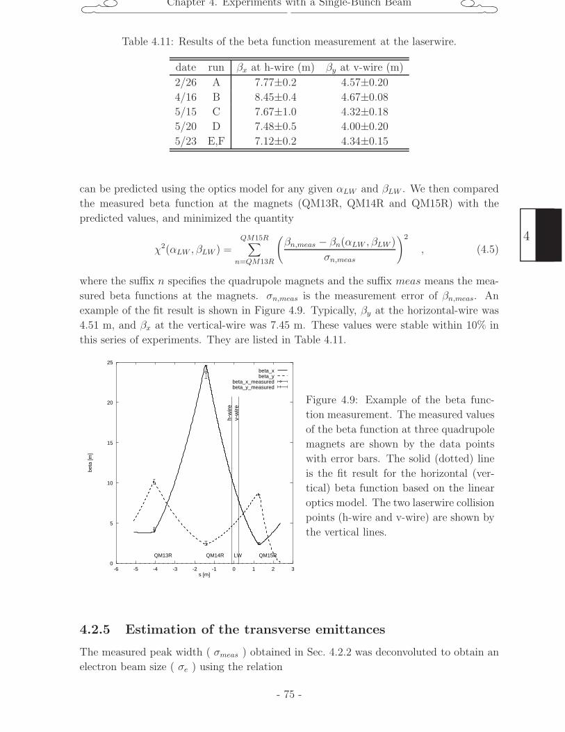
Chapter 4. Experiments with a Single-Bunch Beam
Table 4.11: Results of the beta function measurement at the laserwire.
date run βx at h-wire (m) βy at v-wire (m)
2/26 A 7.77±0.2 4.57±0.20
4/16 B 8.45±0.4 4.67±0.08
5/15 C 7.67±1.0 4.32±0.18
5/20 D 7.48±0.5 4.00±0.20
5/23 E,F 7.12±0.2 4.34±0.15
can be predicted using the optics model for any given αLW and βLW . We then compared
the measured beta function at the magnets (QM13R, QM14R and QM15R) with the
predicted values, and minimized the quantity
χ2(αLW , βLW ) =QM15R∑
n=QM13R
(βn,meas − βn(αLW , βLW )
σn,meas
)2
, (4.5)
where the suffix n specifies the quadrupole magnets and the suffix meas means the mea-
sured beta functions at the magnets. σn,meas is the measurement error of βn,meas. An
example of the fit result is shown in Figure 4.9. Typically, βy at the horizontal-wire was
4.51 m, and βx at the vertical-wire was 7.45 m. These values were stable within 10% in
this series of experiments. They are listed in Table 4.11.
0
5
10
15
20
25
-6 -5 -4 -3 -2 -1 0 1 2 3
beta
[m]
s [m]
QM13R QM14R QM15RLW
beta_xbeta_y
beta_x_measuredbeta_y_measured
v-w
ireh-
wire
Figure 4.9: Example of the beta func-
tion measurement. The measured values
of the beta function at three quadrupole
magnets are shown by the data points
with error bars. The solid (dotted) line
is the fit result for the horizontal (ver-
tical) beta function based on the linear
optics model. The two laserwire collision
points (h-wire and v-wire) are shown by
the vertical lines.
4.2.5 Estimation of the transverse emittances
The measured peak width ( σmeas ) obtained in Sec. 4.2.2 was deconvoluted to obtain an
electron beam size ( σe ) using the relation
- 75 -
4

Chapter 4. Experiments with a Single-Bunch Beam
σe =√σ2
meas − σ2lw (4.6)
where σlw stands for the laserwire width. In Sec.3.4, this was estimated to be σlw(h-wire) =
5.65 ± 0.08 µm and σlw(v-wire) = 14.72 ± 0.24 µm. Then the electron beam size was
converted into an emittance, using the measured beta function, by
σe =√βε . (4.7)
The error on σe has contributions from errors on σmeas, σlw and β. Among them, the
errors on σmeas are individual errors associated with each measurement. The errors on
σlw or β, however, is a common error to all data points within a single run. Below, we do
not include those common errors in a plot because we would be able to see more clearly
the trend or character of the data within a run. At the final stage where comparison
between runs is needed, those common errors will be included.
Figure 4.10 ∼ 4.15 show the plot of the emittances as a function of the ring current.
The solid and dashed lines in the plots show the fitting results by two kinds of empirical
functions, which will be explained in Sec. 4.3.1. As seen in Figure 4.11 (run B) or 4.13 (run
D), the data of the best-tuned beam, the vertical emittance reached as small as 4 pm·rad.
Also clearly seen is the current dependence for both vertical and horizontal directions.
In particular, for the vertical emittance, these are the first data which unambiguously
proved the current dependence.
4.2.6 Measurement of the bunch length
The bunch length of the electron beam was measured by a streak camera. It actually
measured the pulse length of the synchrotron light. One example is shown in Figure 4.16.
In the figure, the vertical axis corresponds to the time structure, and the horizontal axis
to the horizontal profile of the SR light. We defined an area for the synchrotron light
signal to be inside the box in Figure 4.16. The signal intensity distribution was projected
into the time axis, and was fitted by a Gaussian function to estimate the size on the CCD
camera. The bunch length was calculated using the calibration factor of the time axis
(1.85 [pixel/psec] ). Prior to the measurement, we checked the focusing condition without
a sweep signal for the time axis. The input light was found to be well focused on the
photo-cathode, as shown in Figure 4.17. It was confirmed that the signal width without
the sweep was negligible compared to an actual time structure by the beam.
We took three sets of the bunch length data corresponding to the ring conditions of
run D, E and F. Actually, those data were taken on May 23, the last day of this series of
runs, reproducing the respective ring conditions.
The data were continuously taken using a stored beam every ∼7 seconds, and were
classified according to the beam current of every 0.5 mA. The results of three data sets
(denoted as D’, E’, F’) are shown in Figure 4.18. The errors were defined to be the fluctu-
ation of the results (rms). A linear function was employed to fit the current dependence
of the data.
4
- 76 -
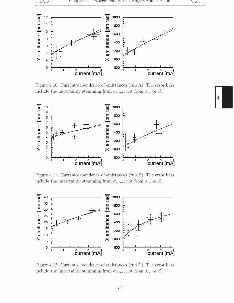
Chapter 4. Experiments with a Single-Bunch Beam
current [mA] current [mA]
Y e
mitt
ance
[pm
rad
]
X e
mitt
ance
[pm
rad
]
Figure 4.10: Current dependence of emittances (run A). The error bars
include the uncertainty stemming from σmeas, not from σlw or β.
current [mA] current [mA]
Y e
mitt
ance
[pm
rad
]
X e
mitt
ance
[pm
rad
]
Figure 4.11: Current dependence of emittances (run B). The error bars
include the uncertainty stemming from σmeas, not from σlw or β.
current [mA] current [mA]
Y e
mitt
ance
[pm
rad
]
X e
mitt
ance
[pm
rad
]
Figure 4.12: Current dependence of emittances (run C). The error bars
include the uncertainty stemming from σmeas, not from σlw or β.
- 77 -
4
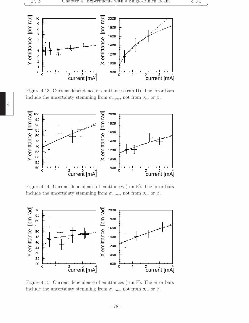
Chapter 4. Experiments with a Single-Bunch Beam
current [mA] current [mA]
Y e
mitt
ance
[pm
rad
]
X e
mitt
ance
[pm
rad
]
Figure 4.13: Current dependence of emittances (run D). The error bars
include the uncertainty stemming from σmeas, not from σlw or β.
current [mA] current [mA]
Y e
mitt
ance
[pm
rad
]
X e
mitt
ance
[pm
rad
]
Figure 4.14: Current dependence of emittances (run E). The error bars
include the uncertainty stemming from σmeas, not from σlw or β.
current [mA] current [mA]
Y e
mitt
ance
[pm
rad
]
X e
mitt
ance
[pm
rad
]
Figure 4.15: Current dependence of emittances (run F). The error bars
include the uncertainty stemming from σmeas, not from σlw or β.
4
- 78 -
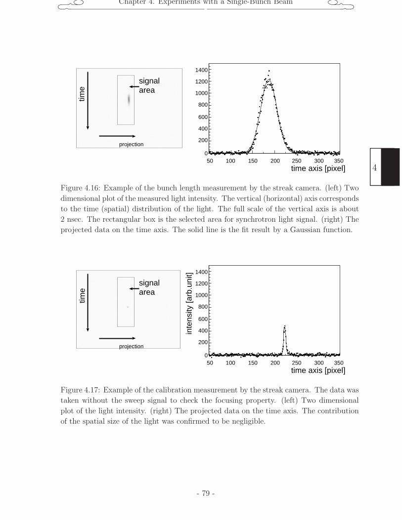
Chapter 4. Experiments with a Single-Bunch Beam
projection
signalarea
time
50 100 150 200 250 300 350
1400
1200
1000
800
600
400
200
0
time axis [pixel]
Figure 4.16: Example of the bunch length measurement by the streak camera. (left) Two
dimensional plot of the measured light intensity. The vertical (horizontal) axis corresponds
to the time (spatial) distribution of the light. The full scale of the vertical axis is about
2 nsec. The rectangular box is the selected area for synchrotron light signal. (right) The
projected data on the time axis. The solid line is the fit result by a Gaussian function.
50 100 150 200 250 300 350
1400
1200
1000
800
600
400
200
0
projection
signalarea
time
inte
nsity
[arb
.uni
t]
time axis [pixel]
Figure 4.17: Example of the calibration measurement by the streak camera. The data was
taken without the sweep signal to check the focusing property. (left) Two dimensional
plot of the light intensity. (right) The projected data on the time axis. The contribution
of the spatial size of the light was confirmed to be negligible.
- 79 -
4
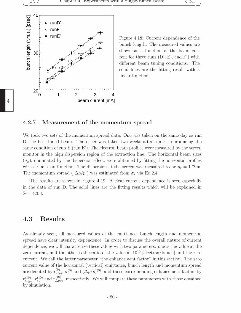
Chapter 4. Experiments with a Single-Bunch Beam
40
30
20 0 1 2 3 4
beam current [mA]
bunc
h le
ngth
(r.
m.s
.) [p
sec]
runD’
runF’
runE’ Figure 4.18: Current dependence of the
bunch length. The measured values are
shown as a function of the beam cur-
rent for three runs (D’, E’, and F’) with
different beam tuning conditions. The
solid lines are the fitting result with a
linear function.
4.2.7 Measurement of the momentum spread
We took two sets of the momentum spread data. One was taken on the same day as run
D, the best-tuned beam. The other was taken two weeks after run E, reproducing the
same condition of run E (run E’). The electron beam profiles were measured by the screen
monitor in the high dispersion region of the extraction line. The horizontal beam sizes
(σx), dominated by the dispersion effect, were obtained by fitting the horizontal profiles
with a Gaussian function. The dispersion at the screen was measured to be ηx = 1.79m.
The momentum spread ( ∆p/p ) was estimated from σx via Eq.2.4.
The results are shown in Figure 4.19. A clear current dependence is seen especially
in the data of run D. The solid lines are the fitting results which will be explained in
Sec. 4.3.3.
4.3 Results
As already seen, all measured values of the emittance, bunch length and momentum
spread have clear intensity dependence. In order to discuss the overall nature of current
dependence, we will characterize these values with two parameters: one is the value at the
zero current, and the other is the ratio of the value at 1010 [electron/bunch] and the zero
current. We call the latter parameter “the enhancement factor” in this section. The zero
current value of the horizontal (vertical) emittance, bunch length and momentum spread
are denoted by ε(0)x(y), σ
(0)z and (∆p/p)(0), and those corresponding enhancement factors by
r(10)εx(y)
, r(10)σz
and r(10)∆p/p, respectively. We will compare these parameters with those obtained
by simulation.
4
- 80 -
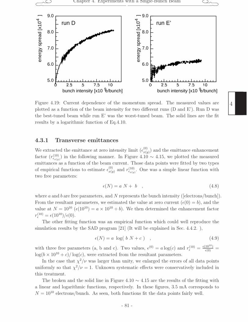
Chapter 4. Experiments with a Single-Bunch Beam
bunch intensity [x10 e/bunch]9 bunch intensity [x10 e/bunch]9
ener
gy s
prea
d [x
10
]-4
9.0
8.0
7.0
6.0
5.0
9.0
8.0
7.0
6.0
5.0
ener
gy s
prea
d [x
10
]-4run D run E’
Figure 4.19: Current dependence of the momentum spread. The measured values are
plotted as a function of the beam intensity for two different runs (D and E’). Run D was
the best-tuned beam while run E’ was the worst-tuned beam. The solid lines are the fit
results by a logarithmic function of Eq.4.10.
4.3.1 Transverse emittances
We extracted the emittance at zero intensity limit (ε(0)x(y)) and the emittance enhancement
factor (r(10)εx(y)
) in the following manner. In Figure 4.10 ∼ 4.15, we plotted the measured
emittances as a function of the beam current. Those data points were fitted by two types
of empirical functions to estimate ε(0)x(y) and r(10)
εx(y). One was a simple linear function with
two free parameters:
ε(N) = a N + b , (4.8)
where a and b are free parameters, andN represents the bunch intensity ([electrons/bunch]).
From the resultant parameters, we estimated the value at zero current (ε(0) = b), and the
value at N = 1010 (ε(1010) = a× 1010 + b). We then determined the enhancement factor
r(10)ε = ε(1010)/ε(0).
The other fitting function was an empirical function which could well reproduce the
simulation results by the SAD program [21] (It will be explained in Sec. 4.4.2. ),
ε(N) = a log( b N + c ) , (4.9)
with three free parameters (a, b and c). Two values, ε(0) = a log(c) and r(10)ε = ε(1010)
ε(0)=
log(b× 1010 + c)/ log(c), were extracted from the resultant parameters.
In the case that χ2/ν was larger than unity, we enlarged the errors of all data points
uniformly so that χ2/ν = 1. Unknown systematic effects were conservatively included in
this treatment.
The broken and the solid line in Figure 4.10 ∼ 4.15 are the results of the fitting with
a linear and logarithmic functions, respectively. In these figures, 3.5 mA corresponds to
N = 1010 electrons/bunch. As seen, both functions fit the data points fairly well.
- 81 -
4
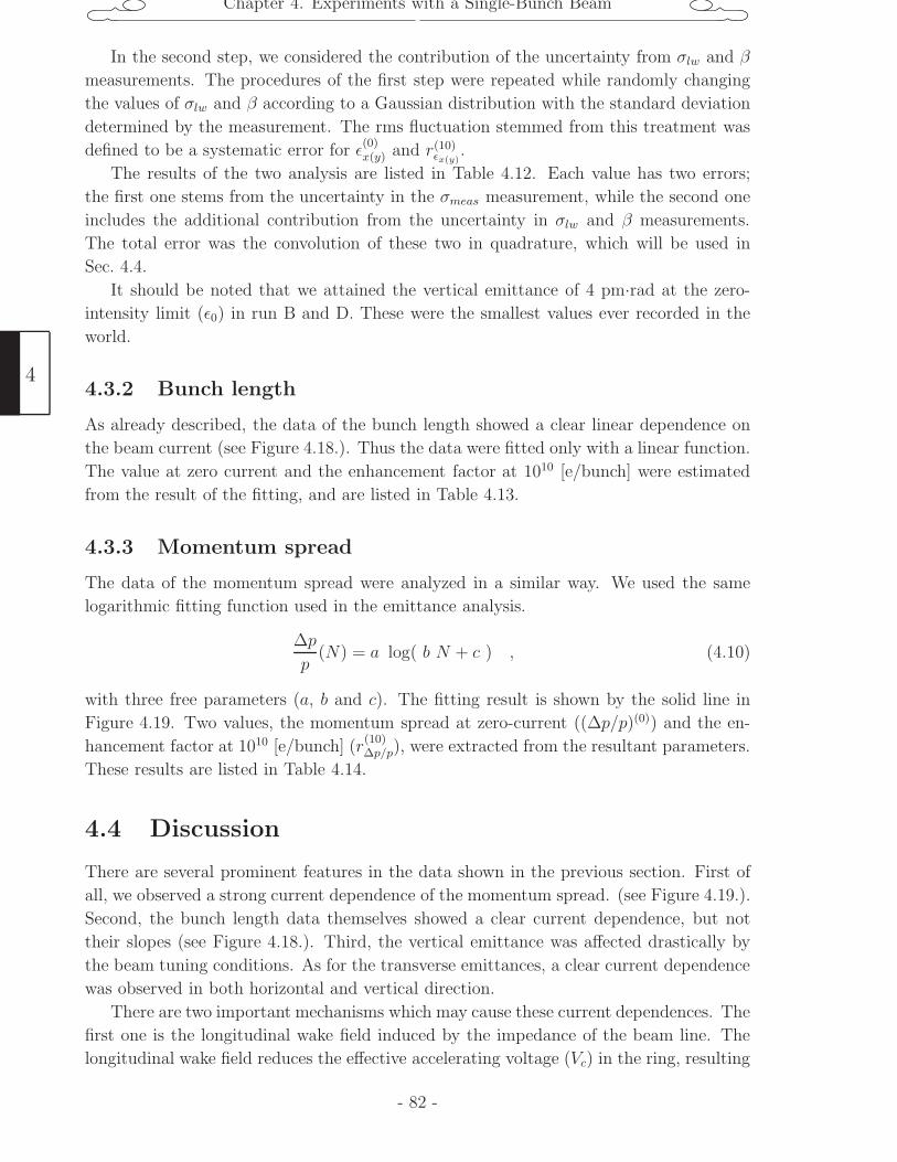
Chapter 4. Experiments with a Single-Bunch Beam
In the second step, we considered the contribution of the uncertainty from σlw and β
measurements. The procedures of the first step were repeated while randomly changing
the values of σlw and β according to a Gaussian distribution with the standard deviation
determined by the measurement. The rms fluctuation stemmed from this treatment was
defined to be a systematic error for ε(0)x(y) and r(10)
εx(y).
The results of the two analysis are listed in Table 4.12. Each value has two errors;
the first one stems from the uncertainty in the σmeas measurement, while the second one
includes the additional contribution from the uncertainty in σlw and β measurements.
The total error was the convolution of these two in quadrature, which will be used in
Sec. 4.4.
It should be noted that we attained the vertical emittance of 4 pm·rad at the zero-
intensity limit (ε0) in run B and D. These were the smallest values ever recorded in the
world.
4.3.2 Bunch length
As already described, the data of the bunch length showed a clear linear dependence on
the beam current (see Figure 4.18.). Thus the data were fitted only with a linear function.
The value at zero current and the enhancement factor at 1010 [e/bunch] were estimated
from the result of the fitting, and are listed in Table 4.13.
4.3.3 Momentum spread
The data of the momentum spread were analyzed in a similar way. We used the same
logarithmic fitting function used in the emittance analysis.
∆p
p(N) = a log( b N + c ) , (4.10)
with three free parameters (a, b and c). The fitting result is shown by the solid line in
Figure 4.19. Two values, the momentum spread at zero-current ((∆p/p)(0)) and the en-
hancement factor at 1010 [e/bunch] (r(10)∆p/p), were extracted from the resultant parameters.
These results are listed in Table 4.14.
4.4 Discussion
There are several prominent features in the data shown in the previous section. First of
all, we observed a strong current dependence of the momentum spread. (see Figure 4.19.).
Second, the bunch length data themselves showed a clear current dependence, but not
their slopes (see Figure 4.18.). Third, the vertical emittance was affected drastically by
the beam tuning conditions. As for the transverse emittances, a clear current dependence
was observed in both horizontal and vertical direction.
There are two important mechanisms which may cause these current dependences. The
first one is the longitudinal wake field induced by the impedance of the beam line. The
longitudinal wake field reduces the effective accelerating voltage (Vc) in the ring, resulting
4
- 82 -
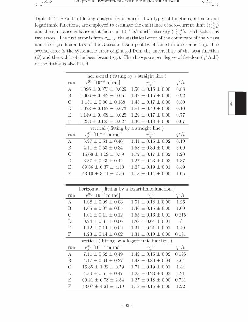
Chapter 4. Experiments with a Single-Bunch Beam
Table 4.12: Results of fitting analysis (emittance). Two types of functions, a linear and
logarithmic functions, are employed to estimate the emittance of zero-current limit (ε(0)x(y))
and the emittance enhancement factor at 1010 [e/bunch] intensity (r(10)εx(y)
). Each value has
two errors. The first error is from σmeas, the statistical error of the count rate of the γ rays
and the reproducibilities of the Gaussian beam profiles obtained in one round trip. The
second error is the systematic error originated from the uncertainty of the beta function
(β) and the width of the laser beam (σlw). The chi-square per degree of freedom (χ2/ndf)
of the fitting is also listed.
horizontal ( fitting by a straight line )
run ε(0)x [10−9 m rad] r(10)εx
χ2/ν
A 1.096 ± 0.073 ± 0.029 1.50 ± 0.16 ± 0.00 0.83
B 1.066 ± 0.062 ± 0.051 1.47 ± 0.15 ± 0.00 0.92
C 1.131 ± 0.86 ± 0.158 1.45 ± 0.17 ± 0.00 0.30
D 1.073 ± 0.167 ± 0.073 1.81 ± 0.49 ± 0.00 0.10
E 1.149 ± 0.099 ± 0.025 1.29 ± 0.17 ± 0.00 0.77
F 1.253 ± 0.123 ± 0.027 1.30 ± 0.18 ± 0.00 0.07
vertical ( fitting by a straight line )
run ε(0)y [10−12 m rad] r(10)εy
χ2/ν
A 6.97 ± 0.53 ± 0.46 1.41 ± 0.16 ± 0.02 0.19
B 4.11 ± 0.53 ± 0.34 1.53 ± 0.30 ± 0.05 3.09
C 16.68 ± 1.09 ± 0.79 1.72 ± 0.17 ± 0.02 1.20
D 3.87 ± 0.43 ± 0.44 1.27 ± 0.23 ± 0.03 1.87
E 69.86 ± 6.37 ± 4.13 1.27 ± 0.19 ± 0.01 0.49
F 43.10 ± 3.71 ± 2.56 1.13 ± 0.14 ± 0.00 1.05
horizontal ( fitting by a logarithmic function )
run ε(0)x [10−9 m rad] r(10)εx
χ2/ν
A 1.08 ± 0.09 ± 0.03 1.51 ± 0.18 ± 0.00 1.26
B 1.05 ± 0.07 ± 0.05 1.46 ± 0.15 ± 0.00 1.09
C 1.01 ± 0.11 ± 0.12 1.55 ± 0.16 ± 0.02 0.215
D 0.94 ± 0.31 ± 0.06 1.88 ± 0.64 ± 0.01 /
E 1.12 ± 0.14 ± 0.02 1.31 ± 0.21 ± 0.01 1.49
F 1.23 ± 0.14 ± 0.02 1.31 ± 0.19 ± 0.00 0.181
vertical ( fitting by a logarithmic function )
run ε(0)y [10−12 m rad] r(10)εy
χ2/ν
A 7.11 ± 0.62 ± 0.49 1.42 ± 0.16 ± 0.02 0.195
B 4.47 ± 0.64 ± 0.37 1.48 ± 0.30 ± 0.04 3.64
C 16.85 ± 1.32 ± 0.79 1.71 ± 0.19 ± 0.01 1.44
D 4.30 ± 0.51 ± 0.47 1.23 ± 0.23 ± 0.03 2.21
E 69.21 ± 6.78 ± 2.34 1.27 ± 0.18 ± 0.00 0.721
F 43.07 ± 4.21 ± 1.49 1.13 ± 0.15 ± 0.00 1.22
- 83 -
4
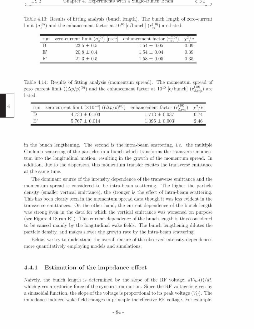
Chapter 4. Experiments with a Single-Bunch Beam
Table 4.13: Results of fitting analysis (bunch length). The bunch length of zero-current
limit (σ(0)z ) and the enhancement factor at 1010 [e/bunch] (r(10)
σz) are listed.
run zero-current limit (σ(0)z ) [psec] enhancement factor (r(10)
σz) χ2/ν
D’ 23.5 ± 0.5 1.54 ± 0.05 0.09
E’ 20.8 ± 0.4 1.54 ± 0.04 0.39
F’ 21.3 ± 0.5 1.58 ± 0.05 0.35
Table 4.14: Results of fitting analysis (momentum spread). The momentum spread of
zero current limit ((∆p/p)(0)) and the enhancement factor at 1010 [e/bunch] (r(10)∆p/p) are
listed.
run zero current limit [×10−4] ((∆p/p)(0)) enhancement factor (r(10)∆p/p) χ2/ν
D 4.730 ± 0.103 1.713 ± 0.037 0.74
E’ 5.767 ± 0.014 1.095 ± 0.003 2.46
in the bunch lengthening. The second is the intra-beam scattering, i.e. the multiple
Coulomb scattering of the particles in a bunch which transforms the transverse momen-
tum into the longitudinal motion, resulting in the growth of the momentum spread. In
addition, due to the dispersion, this momentum transfer excites the transverse emittance
at the same time.
The dominant source of the intensity dependence of the transverse emittance and the
momentum spread is considered to be intra-beam scattering. The higher the particle
density (smaller vertical emittance), the stronger is the effect of intra-beam scattering.
This has been clearly seen in the momentum spread data though it was less evident in the
transverse emittances. On the other hand, the current dependence of the bunch length
was strong even in the data for which the vertical emittance was worsened on purpose
(see Figure 4.18 run E’.). This current dependence of the bunch length is thus considered
to be caused mainly by the longitudinal wake fields. The bunch lengthening dilutes the
particle density, and makes slower the growth rate by the intra-beam scattering.
Below, we try to understand the overall nature of the observed intensity dependences
more quantitatively employing models and simulations.
4.4.1 Estimation of the impedance effect
Naively, the bunch length is determined by the slope of the RF voltage, dVRF (t)/dt,
which gives a restoring force of the synchrotron motion. Since the RF voltage is given by
a sinusoidal function, the slope of the voltage is proportional to its peak voltage (VC). The
impedance-induced wake field changes in principle the effective RF voltage. For example,
4
- 84 -

Chapter 4. Experiments with a Single-Bunch Beam
if the impedance is purely inductive, the wake field can be expressed as
Vw.f. = −LdI(t)
dt(4.11)
where L is the impedance of the beam line and I the beam current. The effective RF
voltage is reduced by Vw.f. in this case. In fact, the calculation based on the structure of
the chambers of the actual beam line suggests a purely inductive impedance. We tried to
include this impedance effect in the SAD simulation program, and to compare its results
with the actual data. Since the impedance effects could not be included directly in SAD,
the impedance effect was simulated by changing the effective RF voltage (Vc).
In order to calculate Vw.f. in Eq. 4.11, we need to know I(t) and L. For I(t), we
employed a parabolic shape, as illustrated in Figure 4.20, for simplicity. It is expressed
by
I(t) =3N
4a
(1 −
(t
a
)2)
, (4.12)
where a represents the bunch length, and N is the total charge. The wake field induced
by this bunch shape is calculated to be
Vw.f. = −LdI(t)
dt= −L3N
2a3t . (4.13)
In this model, the reduction of the effective RF voltage should be proportional to N/σ3z
(σz ∝ a).
t
charge
a-a
~1/aFigure 4.20: Simple model for the lon-
gitudinal bunch shape. The longitudi-
nal charge distribution is expressed by a
parabolic function of Eq. 4.12. In this
model, the bunch length is given by a,
and the total charge is the area under
the parabola.
We now need to determine L, and it was done as follows using the actual bunch length
data. We sought an effective Vc which could reproduce the data. In this procedure, we
were in turn required to assume the x-y coupling, which affected the bunch length. To
this end, we assumed 6% for run D’, 3% for run F’, and 0.4% for run E’, based on the
fact that the ratio of the vertical to horizontal emittance at zero current is 6%, 3%, and
0.4%, respectively for run D, E and F. (See the intersects at zero current in Figure 4.13,
Figure 4.14 and Figure 4.15.)
- 85 -
4
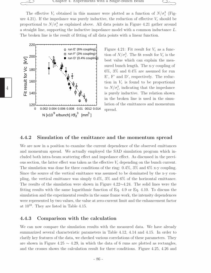
Chapter 4. Experiments with a Single-Bunch Beam
The effective Vc obtained in this manner were plotted as a function of N/σ3z (Fig-
ure 4.21). If the impedance was purely inductive, the reduction of effective Vc should be
proportional to N/σ3z as explained above. All data points in Figure 4.21 gather around
a straight line, supporting the inductive impedance model with a common inductance L.
The broken line is the result of fitting of all data points with a linear function.
220
200
180
160
140
120
Fit
resu
lt fo
r V
c [k
V]
run E’ (6% coupling)run F’ (3% coupling)run D’ (0.4% coupling)
0 0.002 0.004 0.006 0.008 0.01 0012 0.014
N [x10 e/bunch] / [mm ]σz39 3
Figure 4.21: Fit result for Vc as a func-
tion of N/σ3z . The fit result for Vc is the
best value which can explain the mea-
sured bunch length. The x-y coupling of
6%, 3% and 0.4% are assumed for run
E’, F’ and D’, respectively. The reduc-
tion in Vc is found to be proportional
to N/σ3z , indicating that the impedance
is purely inductive. The relation shown
in the broken line is used in the simu-
lation of the emittances and momentum
spread.
4.4.2 Simulation of the emittance and the momentum spread
We are now in a position to examine the current dependence of the observed emittances
and momentum spread. We actually employed the SAD simulation program which in-
cluded both intra-beam scattering effect and impedance effect. As discussed in the previ-
ous section, the latter effect was taken as the effective Vc depending on the bunch current.
The simulation was done for three conditions of the ring: 0.4%, 3% and 6% x-y coupling.
Since the source of the vertical emittance was assumed to be dominated by the x-y cou-
pling, the vertical emittance was simply 0.4%, 3% and 6% of the horizontal emittance.
The results of the simulation were shown in Figure 4.22∼4.24. The solid lines were the
fitting results with the same logarithmic function of Eq. 4.9 or Eq. 4.10. To discuss the
simulation and the experimental results in the same frame work, the intensity dependences
were represented by two values, the value at zero-current limit and the enhancement factor
at 1010. They are listed in Table 4.15.
4.4.3 Comparison with the calculation
We can now compare the simulation results with the measured data. We have already
summarized several characteristic parameters in Table 4.12, 4.14 and 4.15. In order to
clarify key features of the data, we checked various correlations of these parameters. They
are shown in Figure 4.25 ∼ 4.29, in which the data of 6 runs are plotted as rectangles,
and the crosses shows the calculation result for three conditions. Figure 4.25, 4.26 and
4
- 86 -
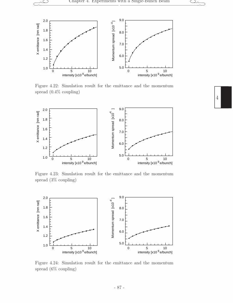
Chapter 4. Experiments with a Single-Bunch Beam
intensity [x10 e/bunch]9
X e
mitt
ance
[nm
rad
]
Mom
entu
m s
prea
d [x
10
]-4
9.0
8.0
7.0
6.0
5.0
2.0
1.8
1.6
1.4
1.2
1.00 5 10 0 5 10
intensity [x10 e/bunch]9
Figure 4.22: Simulation result for the emittance and the momentum
spread (0.4% coupling)
intensity [x10 e/bunch]9
X e
mitt
ance
[nm
rad
]
Mom
entu
m s
prea
d [x
10
]-4
9.0
8.0
7.0
6.0
5.0
2.0
1.8
1.6
1.4
1.2
1.0 0 5 10intensity [x10 e/bunch]9
0 5 10
Figure 4.23: Simulation result for the emittance and the momentum
spread (3% coupling)
intensity [x10 e/bunch]9
X e
mitt
ance
[nm
rad
]
Mom
entu
m s
prea
d [x
10
]-4
9.0
8.0
7.0
6.0
5.0
2.0
1.8
1.6
1.4
1.2
1.00 5 10
intensity [x10 e/bunch]90 5 10
Figure 4.24: Simulation result for the emittance and the momentum
spread (6% coupling)
- 87 -
4
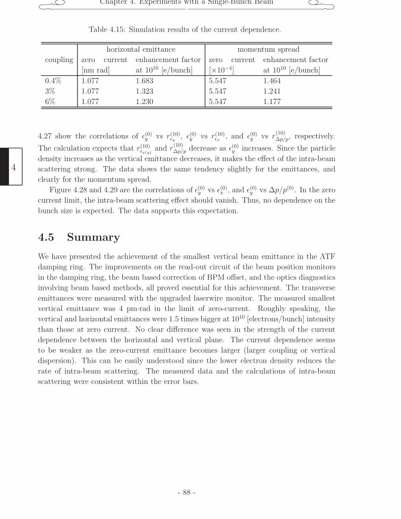
Chapter 4. Experiments with a Single-Bunch Beam
Table 4.15: Simulation results of the current dependence.
horizontal emittance momentum spread
coupling zero current
[nm rad]
enhancement factor
at 1010 [e/bunch]
zero current
[×10−4]
enhancement factor
at 1010 [e/bunch]
0.4% 1.077 1.683 5.547 1.464
3% 1.077 1.323 5.547 1.241
6% 1.077 1.230 5.547 1.177
4.27 show the correlations of ε(0)y vs r(10)εy
, ε(0)y vs r(10)εx
, and ε(0)y vs r(10)∆p/p, respectively.
The calculation expects that r(10)εx(y)
and r(10)∆p/p decrease as ε(0)y increases. Since the particle
density increases as the vertical emittance decreases, it makes the effect of the intra-beam
scattering strong. The data shows the same tendency slightly for the emittances, and
clearly for the momentum spread.
Figure 4.28 and 4.29 are the correlations of ε(0)y vs ε(0)x , and ε(0)y vs ∆p/p(0). In the zero
current limit, the intra-beam scattering effect should vanish. Thus, no dependence on the
bunch size is expected. The data supports this expectation.
4.5 Summary
We have presented the achievement of the smallest vertical beam emittance in the ATF
damping ring. The improvements on the read-out circuit of the beam position monitors
in the damping ring, the beam based correction of BPM offset, and the optics diagnostics
involving beam based methods, all proved essential for this achievement. The transverse
emittances were measured with the upgraded laserwire monitor. The measured smallest
vertical emittance was 4 pm·rad in the limit of zero-current. Roughly speaking, the
vertical and horizontal emittances were 1.5 times bigger at 1010 [electrons/bunch] intensity
than those at zero current. No clear difference was seen in the strength of the current
dependence between the horizontal and vertical plane. The current dependence seems
to be weaker as the zero-current emittance becomes larger (larger coupling or vertical
dispersion). This can be easily understood since the lower electron density reduces the
rate of intra-beam scattering. The measured data and the calculations of intra-beam
scattering were consistent within the error bars.
4
- 88 -
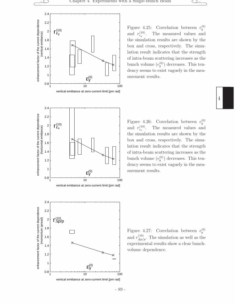
Chapter 4. Experiments with a Single-Bunch Beam
0.8
1
1.2
1.4
1.6
1.8
2
2.2
2.4
1 10 100
vertical emittance at zero-current limit [pm rad]
enha
ncem
ent f
acto
r of
the
curr
ent d
epen
denc
e
(v
ertic
al e
mitt
ance
)
εy(0)
rε(10)
y
Figure 4.25: Correlation between ε(0)y
and r(10)εy
. The measured values and
the simulation results are shown by the
box and cross, respectively. The simu-
lation result indicates that the strength
of intra-beam scattering increases as the
bunch volume (ε(0)y ) decreases. This ten-
dency seems to exist vaguely in the mea-
surement results.
0.8
1
1.2
1.4
1.6
1.8
2
2.2
2.4
1 10 100
vertical emittance at zero-current limit [pm rad]
enha
ncem
ent f
acto
r of
the
curr
ent d
epen
denc
e
(
horiz
onta
l em
ittan
ce)
εy(0)
rε(10)
x
Figure 4.26: Correlation between ε(0)y
and r(10)εx
. The measured values and
the simulation results are shown by the
box and cross, respectively. The simu-
lation result indicates that the strength
of intra-beam scattering increases as the
bunch volume (ε(0)y ) decreases. This ten-
dency seems to exist vaguely in the mea-
surement results.
0.8
1
1.2
1.4
1.6
1.8
2
2.2
2.4
1 10 100
vertical emittance at zero-current limit [pm rad]
enha
ncem
ent f
acto
r of
the
curr
ent d
epen
denc
e
(m
omen
tum
spr
ead)
εy(0)
r∆p/p(10)
Figure 4.27: Correlation between ε(0)y
and r(10)∆p/p. The simulation as well as the
experimental results show a clear bunch-
volume dependence.
- 89 -
4
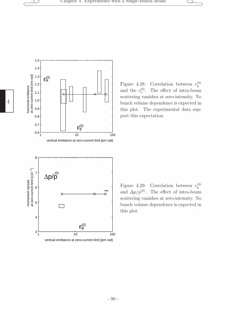
Chapter 4. Experiments with a Single-Bunch Beam
0.6
1.5
1 10 100
vertical emittance at zero-current limit [pm rad]
horiz
onta
l em
ittan
ce
at z
ero-
curr
ent l
imit
[nm
rad
]
1.3
1.1
0.7
0.8
1.4
1.2
1.0
0.9
εy(0)
εx(0)
Figure 4.28: Correlation between ε(0)y
and the ε(0)x . The effect of intra-beam
scattering vanishes at zero-intensity. No
bunch volume dependence is expected in
this plot. The experimental data sup-
port this expectation.
3
8
1 10 100
vertical emittance at zero-current limit [pm rad]
mom
entu
m s
prea
d at
zer
o-cu
rren
t lim
it [x
10
]
4
5
6
7
-4
εy(0)
∆p/p(0)
Figure 4.29: Correlation between ε(0)y
and ∆p/p(0). The effect of intra-beam
scattering vanishes at zero-intensity. No
bunch volume dependence is expected in
this plot.
4
- 90 -
Chapter 5. Experiments with a Multi-Bunch Beam
Chapter 5
Experiments with a Multi-Bunch
Beam
5.1 Introduction
Future linear colliders are designed to use a multi-bunch beam to attain their required
luminosity. Thus, realization of a small emittance in a multi-bunch beam should also be
confirmed experimentally.
In this section, we begin by explaining needed modifications to the laserwire system,
which enable a separate profile measurements for each bunch. Then we present the results
of studies with the multi-bunch beams. We carried out 4 runs in total with the following
purposes:
Run 1 A systematic emittance measurement of a multi-bunch beam ([41]). Both hori-
zontal and vertical emittances were measured, and their bunch-number and intensity
dependence were studied.
Run 2 and 3 A pair of runs to compare the vertical emittances between the single and
multi-bunch modes under a well-tuned ring condition. The two modes were switched
consecutively not to alter other ring conditions.
Run 4 A pressure dependence study. The vacuum pressure was intentionally increased
to study the ion-induced coupled bunch effect.
Table 5.1: Experiments with a multi-bunch beam
date run aim
December 03, 2002 1 bunch-number and intensity dependence
June 06, 2002 2 and 3 comparison with the single bunch mode
June 13,2003 4 pressure dependence study
- 91 -
5
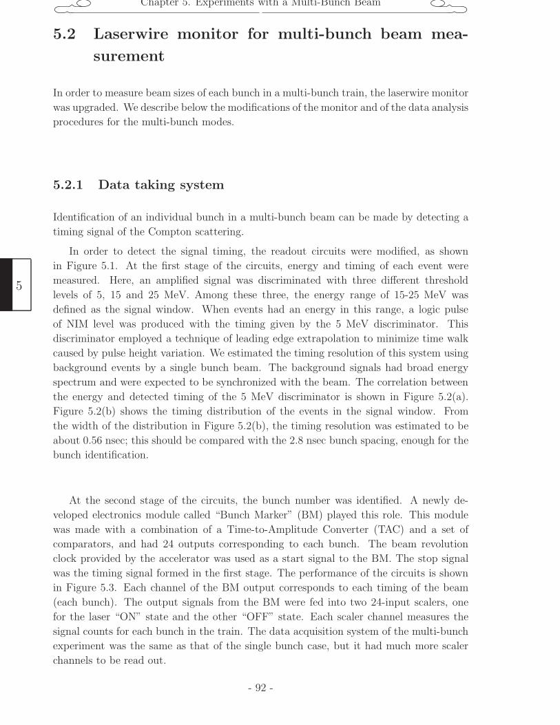
Chapter 5. Experiments with a Multi-Bunch Beam
5.2 Laserwire monitor for multi-bunch beam mea-
surement
In order to measure beam sizes of each bunch in a multi-bunch train, the laserwire monitor
was upgraded. We describe below the modifications of the monitor and of the data analysis
procedures for the multi-bunch modes.
5.2.1 Data taking system
Identification of an individual bunch in a multi-bunch beam can be made by detecting a
timing signal of the Compton scattering.
In order to detect the signal timing, the readout circuits were modified, as shown
in Figure 5.1. At the first stage of the circuits, energy and timing of each event were
measured. Here, an amplified signal was discriminated with three different threshold
levels of 5, 15 and 25 MeV. Among these three, the energy range of 15-25 MeV was
defined as the signal window. When events had an energy in this range, a logic pulse
of NIM level was produced with the timing given by the 5 MeV discriminator. This
discriminator employed a technique of leading edge extrapolation to minimize time walk
caused by pulse height variation. We estimated the timing resolution of this system using
background events by a single bunch beam. The background signals had broad energy
spectrum and were expected to be synchronized with the beam. The correlation between
the energy and detected timing of the 5 MeV discriminator is shown in Figure 5.2(a).
Figure 5.2(b) shows the timing distribution of the events in the signal window. From
the width of the distribution in Figure 5.2(b), the timing resolution was estimated to be
about 0.56 nsec; this should be compared with the 2.8 nsec bunch spacing, enough for the
bunch identification.
At the second stage of the circuits, the bunch number was identified. A newly de-
veloped electronics module called “Bunch Marker” (BM) played this role. This module
was made with a combination of a Time-to-Amplitude Converter (TAC) and a set of
comparators, and had 24 outputs corresponding to each bunch. The beam revolution
clock provided by the accelerator was used as a start signal to the BM. The stop signal
was the timing signal formed in the first stage. The performance of the circuits is shown
in Figure 5.3. Each channel of the BM output corresponds to each timing of the beam
(each bunch). The output signals from the BM were fed into two 24-input scalers, one
for the laser “ON” state and the other “OFF” state. Each scaler channel measures the
signal counts for each bunch in the train. The data acquisition system of the multi-bunch
experiment was the same as that of the single bunch case, but it had much more scaler
channels to be read out.
5
- 92 -
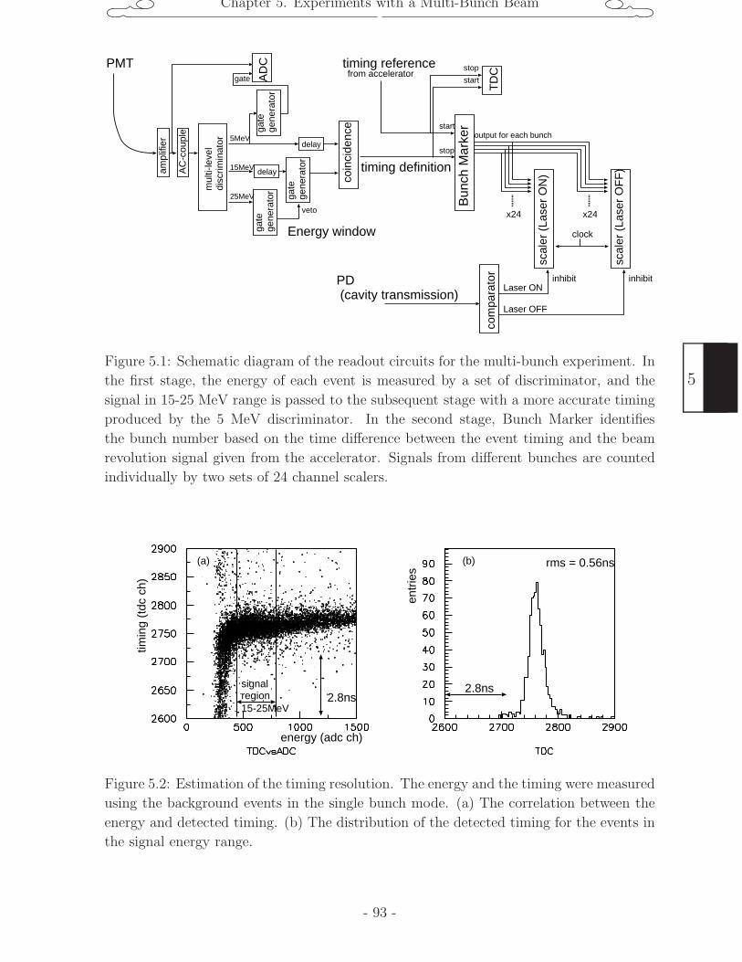
Chapter 5. Experiments with a Multi-Bunch Beam
Bun
ch M
arke
r
timing definition
output for each bunch
timing reference
x24 x24
scal
er (
Lase
r O
N)
scal
er (
Lase
r O
FF
)
PD (cavity transmission)
com
para
tor
inhibit inhibitLaser ON
Laser OFF
TD
C
start
stop
start
stop
coin
cide
nce
mul
ti-le
vel
disc
rimin
ator delay
gate
gene
rato
r
veto
gate
gene
rato
r
delay
Energy window
PMT
AC
-cou
ple
ampl
ifier
from accelerator
5MeV
15MeV
25MeV
clock
AD
Cga
tege
nera
tor
gate
Figure 5.1: Schematic diagram of the readout circuits for the multi-bunch experiment. In
the first stage, the energy of each event is measured by a set of discriminator, and the
signal in 15-25 MeV range is passed to the subsequent stage with a more accurate timing
produced by the 5 MeV discriminator. In the second stage, Bunch Marker identifies
the bunch number based on the time difference between the event timing and the beam
revolution signal given from the accelerator. Signals from different bunches are counted
individually by two sets of 24 channel scalers.
2.8ns
rms = 0.56ns
entr
ies
energy (adc ch)
timin
g (t
dc c
h)
2.8nssignalregion15-25MeV
(a) (b)
Figure 5.2: Estimation of the timing resolution. The energy and the timing were measured
using the background events in the single bunch mode. (a) The correlation between the
energy and detected timing. (b) The distribution of the detected timing for the events in
the signal energy range.
- 93 -
5
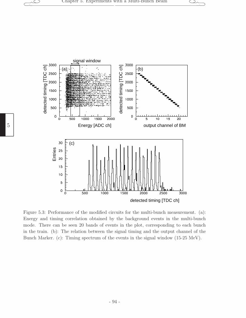
Chapter 5. Experiments with a Multi-Bunch Beam
dete
cted
tim
ing
[TD
C c
h]
dete
cted
tim
ing
[TD
C c
h]Energy [ADC ch] output channel of BM
signal window
detected timing [TDC ch]
Ent
ries
(a) (b)
(c)
Figure 5.3: Performance of the modified circuits for the multi-bunch measurement. (a):
Energy and timing correlation obtained by the background events in the multi-bunch
mode. There can be seen 20 bands of events in the plot, corresponding to each bunch
in the train. (b): The relation between the signal timing and the output channel of the
Bunch Marker. (c): Timing spectrum of the events in the signal window (15-25 MeV).
5
- 94 -
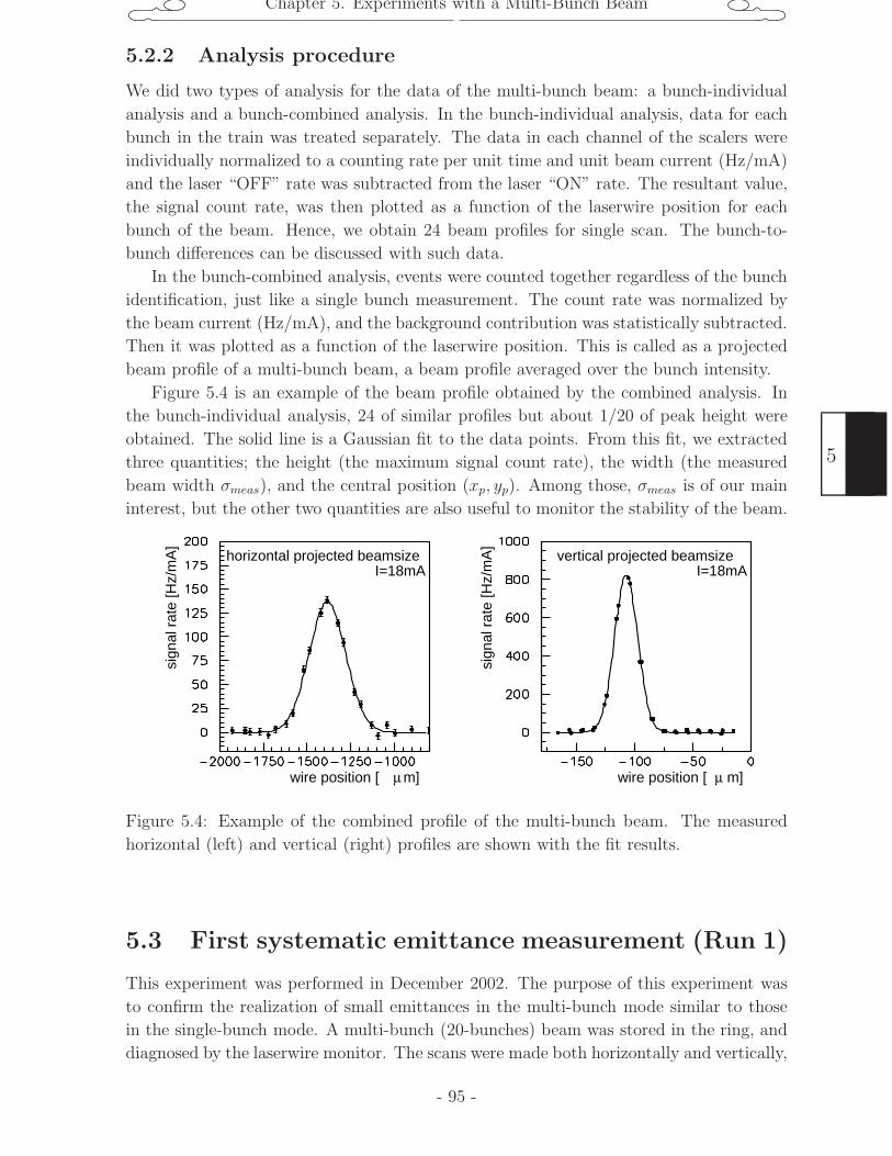
Chapter 5. Experiments with a Multi-Bunch Beam
5.2.2 Analysis procedure
We did two types of analysis for the data of the multi-bunch beam: a bunch-individual
analysis and a bunch-combined analysis. In the bunch-individual analysis, data for each
bunch in the train was treated separately. The data in each channel of the scalers were
individually normalized to a counting rate per unit time and unit beam current (Hz/mA)
and the laser “OFF” rate was subtracted from the laser “ON” rate. The resultant value,
the signal count rate, was then plotted as a function of the laserwire position for each
bunch of the beam. Hence, we obtain 24 beam profiles for single scan. The bunch-to-
bunch differences can be discussed with such data.
In the bunch-combined analysis, events were counted together regardless of the bunch
identification, just like a single bunch measurement. The count rate was normalized by
the beam current (Hz/mA), and the background contribution was statistically subtracted.
Then it was plotted as a function of the laserwire position. This is called as a projected
beam profile of a multi-bunch beam, a beam profile averaged over the bunch intensity.
Figure 5.4 is an example of the beam profile obtained by the combined analysis. In
the bunch-individual analysis, 24 of similar profiles but about 1/20 of peak height were
obtained. The solid line is a Gaussian fit to the data points. From this fit, we extracted
three quantities; the height (the maximum signal count rate), the width (the measured
beam width σmeas), and the central position (xp, yp). Among those, σmeas is of our main
interest, but the other two quantities are also useful to monitor the stability of the beam.
horizontal projected beamsize vertical projected beamsize
sign
al r
ate
[Hz/
mA
]
sign
al r
ate
[Hz/
mA
]
wire position [ m] wire position [ m]
I=18mA I=18mA
µ µ
Figure 5.4: Example of the combined profile of the multi-bunch beam. The measured
horizontal (left) and vertical (right) profiles are shown with the fit results.
5.3 First systematic emittance measurement (Run 1)
This experiment was performed in December 2002. The purpose of this experiment was
to confirm the realization of small emittances in the multi-bunch mode similar to those
in the single-bunch mode. A multi-bunch (20-bunches) beam was stored in the ring, and
diagnosed by the laserwire monitor. The scans were made both horizontally and vertically,
- 95 -
5
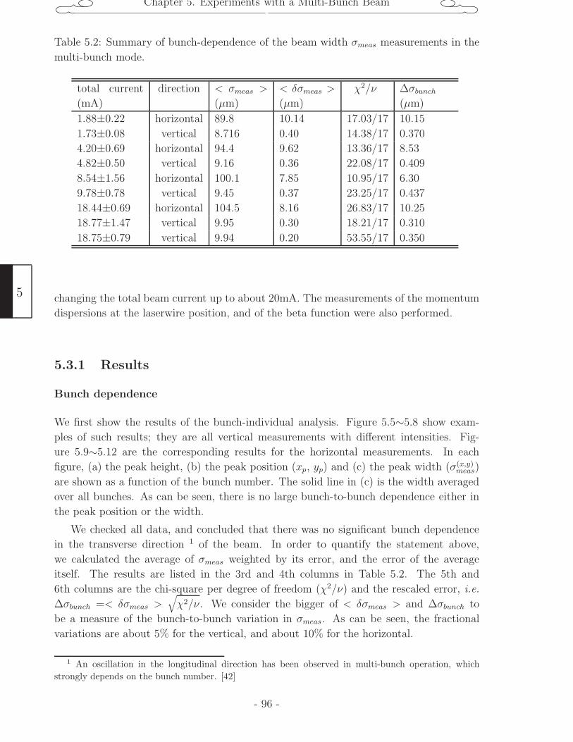
Chapter 5. Experiments with a Multi-Bunch Beam
Table 5.2: Summary of bunch-dependence of the beam width σmeas measurements in the
multi-bunch mode.
total current
(mA)
direction < σmeas >
(µm)
< δσmeas >
(µm)
χ2/ν ∆σbunch
(µm)
1.88±0.22 horizontal 89.8 10.14 17.03/17 10.15
1.73±0.08 vertical 8.716 0.40 14.38/17 0.370
4.20±0.69 horizontal 94.4 9.62 13.36/17 8.53
4.82±0.50 vertical 9.16 0.36 22.08/17 0.409
8.54±1.56 horizontal 100.1 7.85 10.95/17 6.30
9.78±0.78 vertical 9.45 0.37 23.25/17 0.437
18.44±0.69 horizontal 104.5 8.16 26.83/17 10.25
18.77±1.47 vertical 9.95 0.30 18.21/17 0.310
18.75±0.79 vertical 9.94 0.20 53.55/17 0.350
changing the total beam current up to about 20mA. The measurements of the momentum
dispersions at the laserwire position, and of the beta function were also performed.
5.3.1 Results
Bunch dependence
We first show the results of the bunch-individual analysis. Figure 5.5∼5.8 show exam-
ples of such results; they are all vertical measurements with different intensities. Fig-
ure 5.9∼5.12 are the corresponding results for the horizontal measurements. In each
figure, (a) the peak height, (b) the peak position (xp, yp) and (c) the peak width (σ(x,y)meas)
are shown as a function of the bunch number. The solid line in (c) is the width averaged
over all bunches. As can be seen, there is no large bunch-to-bunch dependence either in
the peak position or the width.
We checked all data, and concluded that there was no significant bunch dependence
in the transverse direction 1 of the beam. In order to quantify the statement above,
we calculated the average of σmeas weighted by its error, and the error of the average
itself. The results are listed in the 3rd and 4th columns in Table 5.2. The 5th and
6th columns are the chi-square per degree of freedom (χ2/ν) and the rescaled error, i.e.
∆σbunch =< δσmeas >√χ2/ν. We consider the bigger of < δσmeas > and ∆σbunch to
be a measure of the bunch-to-bunch variation in σmeas. As can be seen, the fractional
variations are about 5% for the vertical, and about 10% for the horizontal.
1 An oscillation in the longitudinal direction has been observed in multi-bunch operation, whichstrongly depends on the bunch number. [42]
5
- 96 -
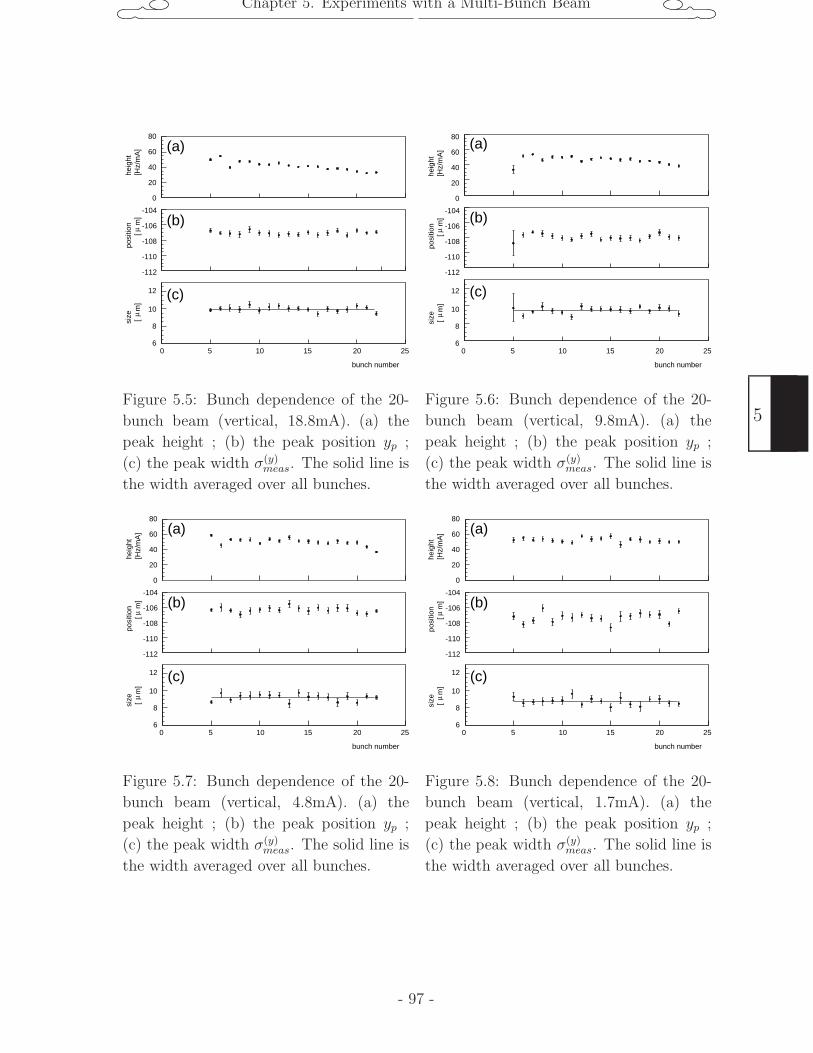
Chapter 5. Experiments with a Multi-Bunch Beam
80
60
40
20
0
-104
-106
-108
-110
-112
12
10
8
6 0 5 10 15 20 25
heig
ht[H
z/m
A]
posi
tion
[ m
]µ
size
[
m]
µ
bunch number
(a)
(b)
(c)
Figure 5.5: Bunch dependence of the 20-
bunch beam (vertical, 18.8mA). (a) the
peak height ; (b) the peak position yp ;
(c) the peak width σ(y)meas. The solid line is
the width averaged over all bunches.
80
60
40
20
0
-104
-106
-108
-110
-112
12
10
8
6 5 10 15 20 25
heig
ht[H
z/m
A]
posi
tion
[ m
]µ
size
[
m]
µ
bunch number
0
(a)
(b)
(c)
Figure 5.6: Bunch dependence of the 20-
bunch beam (vertical, 9.8mA). (a) the
peak height ; (b) the peak position yp ;
(c) the peak width σ(y)meas. The solid line is
the width averaged over all bunches.
80
60
40
20
0
-104
-106
-108
-110
-112
12
10
8
6 5 10 15 20 25
heig
ht[H
z/m
A]
posi
tion
[ m
]µ
size
[
m]
µ
bunch number
0
(a)
(b)
(c)
Figure 5.7: Bunch dependence of the 20-
bunch beam (vertical, 4.8mA). (a) the
peak height ; (b) the peak position yp ;
(c) the peak width σ(y)meas. The solid line is
the width averaged over all bunches.
80
60
40
20
0
-104
-106
-108
-110
-112
12
10
8
6 5 10 15 20 25
heig
ht[H
z/m
A]
posi
tion
[ m
]µ
size
[
m]
µ
bunch number
0
(a)
(b)
(c)
Figure 5.8: Bunch dependence of the 20-
bunch beam (vertical, 1.7mA). (a) the
peak height ; (b) the peak position yp ;
(c) the peak width σ(y)meas. The solid line is
the width averaged over all bunches.
- 97 -
5
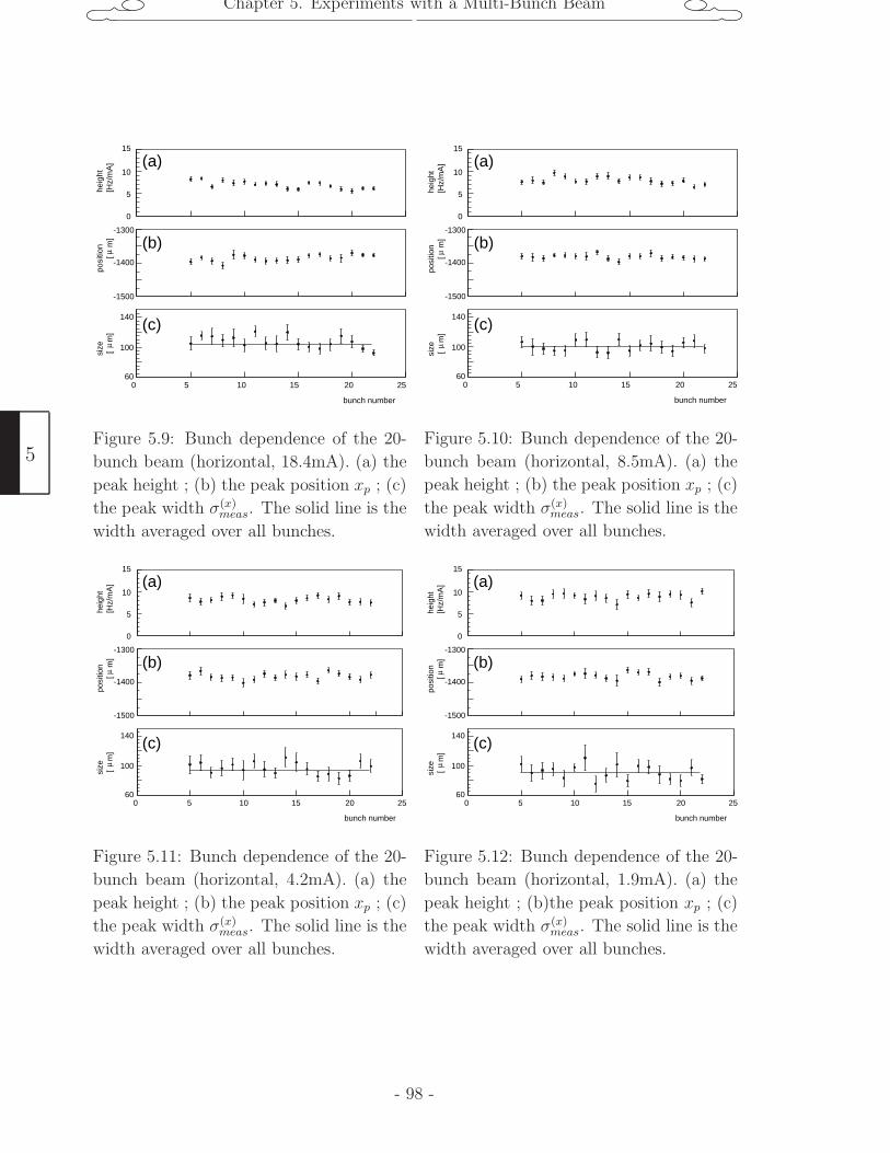
Chapter 5. Experiments with a Multi-Bunch Beam
15
10
5
0
-1300
-1500
140
0 5 10 15 20 25
heig
ht[H
z/m
A]
posi
tion
[ m
]si
ze [
m
]
bunch number
µ
-1400
100
60
µ
(a)
(b)
(c)
Figure 5.9: Bunch dependence of the 20-
bunch beam (horizontal, 18.4mA). (a) the
peak height ; (b) the peak position xp ; (c)
the peak width σ(x)meas. The solid line is the
width averaged over all bunches.
15
10
5
0
-1300
-1500
140
0 5 10 15 20 25
heig
ht[H
z/m
A]
posi
tion
[ m
]si
ze [
m
]
bunch number
µ
-1400
100
60
µ
(a)
(b)
(c)
Figure 5.10: Bunch dependence of the 20-
bunch beam (horizontal, 8.5mA). (a) the
peak height ; (b) the peak position xp ; (c)
the peak width σ(x)meas. The solid line is the
width averaged over all bunches.
15
10
5
0
-1300
-1500
140
5 10 15 20 25
heig
ht[H
z/m
A]
posi
tion
[ m
]si
ze [
m
]
bunch number
µ
-1400
100
60
µ
0
(a)
(b)
(c)
Figure 5.11: Bunch dependence of the 20-
bunch beam (horizontal, 4.2mA). (a) the
peak height ; (b) the peak position xp ; (c)
the peak width σ(x)meas. The solid line is the
width averaged over all bunches.
15
10
5
0
-1300
-1500
140
5 10 15 20 25
heig
ht[H
z/m
A]
posi
tion
[ m
]si
ze [
m
]
bunch number
µ
-1400
100
60
µ
0
(a)
(b)
(c)
Figure 5.12: Bunch dependence of the 20-
bunch beam (horizontal, 1.9mA). (a) the
peak height ; (b)the peak position xp ; (c)
the peak width σ(x)meas. The solid line is the
width averaged over all bunches.
5
- 98 -
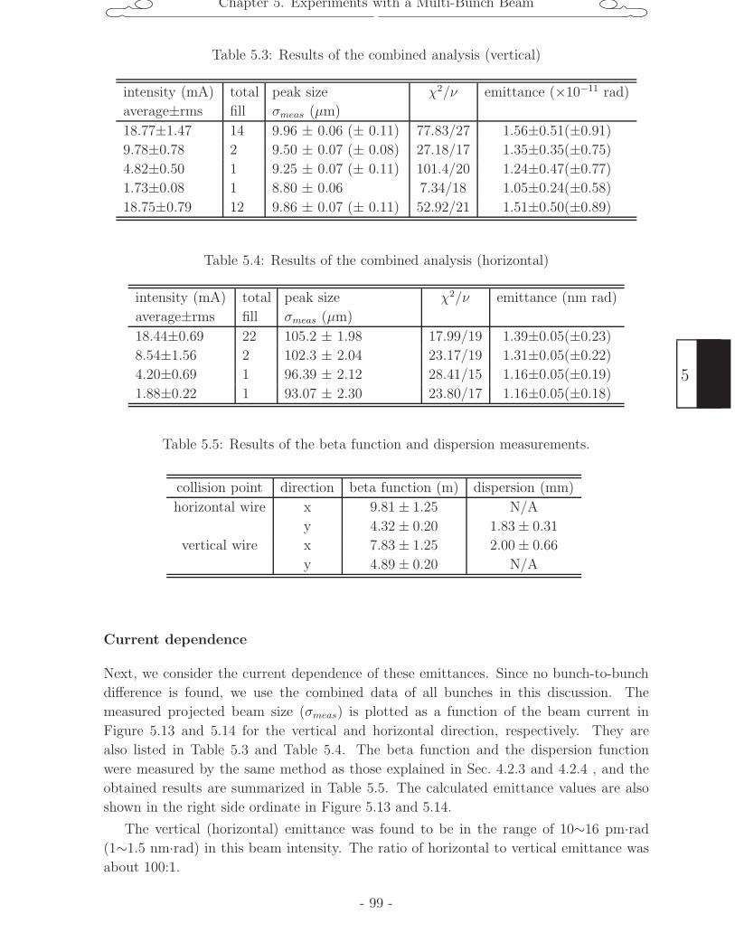
Chapter 5. Experiments with a Multi-Bunch Beam
Table 5.3: Results of the combined analysis (vertical)
intensity (mA)
average±rms
total
fill
peak size
σmeas (µm)
χ2/ν emittance (×10−11 rad)
18.77±1.47 14 9.96 ± 0.06 (± 0.11) 77.83/27 1.56±0.51(±0.91)
9.78±0.78 2 9.50 ± 0.07 (± 0.08) 27.18/17 1.35±0.35(±0.75)
4.82±0.50 1 9.25 ± 0.07 (± 0.11) 101.4/20 1.24±0.47(±0.77)
1.73±0.08 1 8.80 ± 0.06 7.34/18 1.05±0.24(±0.58)
18.75±0.79 12 9.86 ± 0.07 (± 0.11) 52.92/21 1.51±0.50(±0.89)
Table 5.4: Results of the combined analysis (horizontal)
intensity (mA)
average±rms
total
fill
peak size
σmeas (µm)
χ2/ν emittance (nm rad)
18.44±0.69 22 105.2 ± 1.98 17.99/19 1.39±0.05(±0.23)
8.54±1.56 2 102.3 ± 2.04 23.17/19 1.31±0.05(±0.22)
4.20±0.69 1 96.39 ± 2.12 28.41/15 1.16±0.05(±0.19)
1.88±0.22 1 93.07 ± 2.30 23.80/17 1.16±0.05(±0.18)
Table 5.5: Results of the beta function and dispersion measurements.
collision point direction beta function (m) dispersion (mm)
horizontal wire x 9.81 ± 1.25 N/A
y 4.32 ± 0.20 1.83 ± 0.31
vertical wire x 7.83 ± 1.25 2.00 ± 0.66
y 4.89 ± 0.20 N/A
Current dependence
Next, we consider the current dependence of these emittances. Since no bunch-to-bunch
difference is found, we use the combined data of all bunches in this discussion. The
measured projected beam size (σmeas) is plotted as a function of the beam current in
Figure 5.13 and 5.14 for the vertical and horizontal direction, respectively. They are
also listed in Table 5.3 and Table 5.4. The beta function and the dispersion function
were measured by the same method as those explained in Sec. 4.2.3 and 4.2.4 , and the
obtained results are summarized in Table 5.5. The calculated emittance values are also
shown in the right side ordinate in Figure 5.13 and 5.14.
The vertical (horizontal) emittance was found to be in the range of 10∼16 pm·rad
(1∼1.5 nm·rad) in this beam intensity. The ratio of horizontal to vertical emittance was
about 100:1.
- 99 -
5
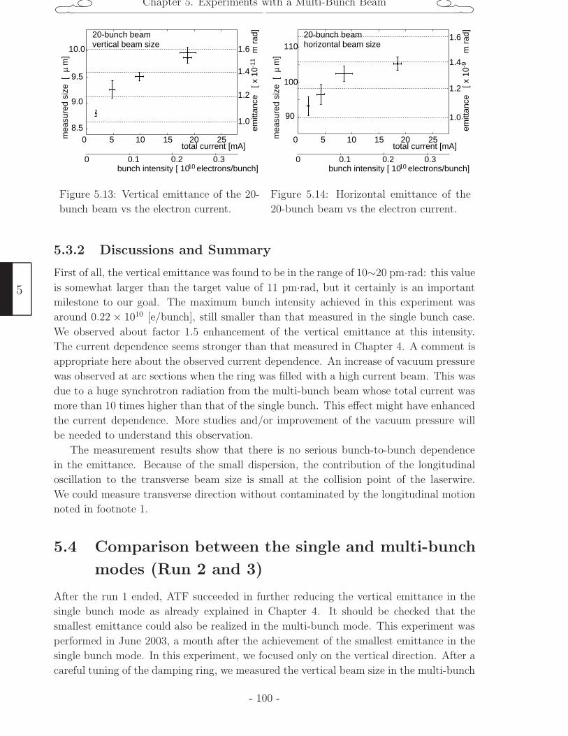
Chapter 5. Experiments with a Multi-Bunch Beam
total current [mA]
mea
sure
d si
ze [
m
]µ
0 0.1 0.2 0.3
0 5 10 15 20 258.5
9.0
9.5
10.0
20-bunch beamvertical beam size
bunch intensity [ 10 electrons/bunch]10
1.6
1.4
1.2
1.0
[ x 1
0
m r
ad]
emitt
ance
-11
Figure 5.13: Vertical emittance of the 20-
bunch beam vs the electron current.
total current [mA]
mea
sure
d si
ze [
m
]µ
0 0.1 0.2 0.3
0 5 10 15 20 25
90
100
20-bunch beamhorizontal beam size
bunch intensity [ 10 electrons/bunch]10
1.6
1.4
1.2
1.0
[ x 1
0
m r
ad]
emitt
ance
-9
110
Figure 5.14: Horizontal emittance of the
20-bunch beam vs the electron current.
5.3.2 Discussions and Summary
First of all, the vertical emittance was found to be in the range of 10∼20 pm·rad: this value
is somewhat larger than the target value of 11 pm·rad, but it certainly is an important
milestone to our goal. The maximum bunch intensity achieved in this experiment was
around 0.22 × 10¹⁰ [e/bunch], still smaller than that measured in the single bunch case.
We observed about factor 1.5 enhancement of the vertical emittance at this intensity.
The current dependence seems stronger than that measured in Chapter 4. A comment is
appropriate here about the observed current dependence. An increase of vacuum pressure
was observed at arc sections when the ring was filled with a high current beam. This was
due to a huge synchrotron radiation from the multi-bunch beam whose total current was
more than 10 times higher than that of the single bunch. This effect might have enhanced
the current dependence. More studies and/or improvement of the vacuum pressure will
be needed to understand this observation.
The measurement results show that there is no serious bunch-to-bunch dependence
in the emittance. Because of the small dispersion, the contribution of the longitudinal
oscillation to the transverse beam size is small at the collision point of the laserwire.
We could measure transverse direction without contaminated by the longitudinal motion
noted in footnote 1.
5.4 Comparison between the single and multi-bunch
modes (Run 2 and 3)
After the run 1 ended, ATF succeeded in further reducing the vertical emittance in the
single bunch mode as already explained in Chapter 4. It should be checked that the
smallest emittance could also be realized in the multi-bunch mode. This experiment was
performed in June 2003, a month after the achievement of the smallest emittance in the
single bunch mode. In this experiment, we focused only on the vertical direction. After a
careful tuning of the damping ring, we measured the vertical beam size in the multi-bunch
5
- 100 -
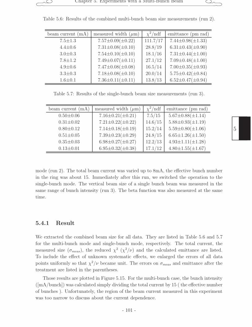
Chapter 5. Experiments with a Multi-Bunch Beam
Table 5.6: Results of the combined multi-bunch beam size measurements (run 2).
beam current (mA) measured width (µm) χ2/ndf emittance (pm rad)
7.5±1.3 7.57±0.09(±0.22) 111.7/17 7.44±0.98(±1.33)
4.4±0.6 7.31±0.08(±0.10) 28.8/19 6.31±0.43(±0.90)
3.0±0.3 7.54±0.10(±0.10) 18.1/16 7.31±0.44(±1.00)
7.8±1.2 7.49±0.07(±0.11) 27.1/12 7.09±0.48(±1.00)
4.9±0.6 7.47±0.08(±0.08) 16.5/14 7.00±0.35(±0.93)
3.3±0.3 7.18±0.08(±0.10) 20.0/14 5.75±0.42(±0.84)
1.6±0.1 7.36±0.11(±0.11) 13.8/13 6.52±0.47(±0.94)
Table 5.7: Results of the single-bunch beam size measurements (run 3).
beam current (mA) measured width (µm) χ2/ndf emittance (pm rad)
0.50±0.06 7.16±0.21(±0.21) 7.5/15 5.67±0.88(±1.14)
0.31±0.02 7.21±0.22(±0.22) 14.6/15 5.88±0.93(±1.19)
0.80±0.12 7.14±0.18(±0.19) 15.2/14 5.59±0.80(±1.06)
0.51±0.05 7.39±0.23(±0.29) 24.8/15 6.65±1.26(±1.50)
0.35±0.03 6.98±0.27(±0.27) 12.2/13 4.93±1.11(±1.28)
0.13±0.01 6.95±0.32(±0.38) 17.1/12 4.80±1.55(±1.67)
mode (run 2). The total beam current was varied up to 8mA, the effective bunch number
in the ring was about 15. Immediately after this run, we switched the operation to the
single-bunch mode. The vertical beam size of a single bunch beam was measured in the
same range of bunch intensity (run 3). The beta function was also measured at the same
time.
5.4.1 Result
We extracted the combined beam size for all data. They are listed in Table 5.6 and 5.7
for the multi-bunch mode and single-bunch mode, respectively. The total current, the
measured size (σmeas), the reduced χ2 (χ2/ν) and the calculated emittance are listed.
To include the effect of unknown systematic effects, we enlarged the errors of all data
points uniformly so that χ2/ν became unit. The errors on σmeas and emittance after the
treatment are listed in the parentheses.
Those results are plotted in Figure 5.15. For the multi-bunch case, the bunch intensity
([mA/bunch]) was calculated simply dividing the total current by 15 ( the effective number
of bunches ). Unfortunately, the region of the beam current measured in this experiment
was too narrow to discuss about the current dependence.
- 101 -
5
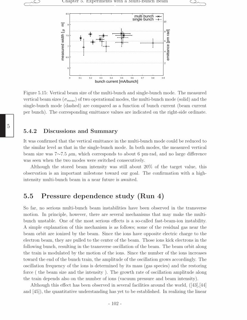
Chapter 5. Experiments with a Multi-Bunch Beam
6
6.5
7
7.5
8
8.5
0 0.1 0.2 0.3 0.4 0.5 0.6 0.7 0.8 0.9
bunch current [mA/bunch]
multi bunchsingle bunch
mea
sure
d w
idth
[
m]
µ2
4
6
8
10
emitt
ance
[pm
rad
]
Figure 5.15: Vertical beam size of the multi-bunch and single-bunch mode. The measured
vertical beam sizes (σmeas) of two operational modes, the multi-bunch mode (solid) and the
single-bunch mode (dashed) are compared as a function of bunch current (beam current
per bunch). The corresponding emittance values are indicated on the right-side ordinate.
5.4.2 Discussions and Summary
It was confirmed that the vertical emittance in the multi-bunch mode could be reduced to
the similar level as that in the single-bunch mode. In both modes, the measured vertical
beam size was 7∼7.5 µm, which corresponds to about 6 pm·rad, and no large difference
was seen when the two modes were switched consecutively.
Although the stored beam intensity was still about 20% of the target value, this
observation is an important milestone toward our goal. The confirmation with a high-
intensity multi-bunch beam in a near future is awaited.
5.5 Pressure dependence study (Run 4)
So far, no serious multi-bunch beam instabilities have been observed in the transverse
motion. In principle, however, there are several mechanisms that may make the multi-
bunch unstable. One of the most serious effects is a so-called fast-beam-ion instability.
A simple explanation of this mechanism is as follows; some of the residual gas near the
beam orbit are ionized by the beam. Since the ions have opposite electric charge to the
electron beam, they are pulled to the center of the beam. Those ions kick electrons in the
following bunch, resulting in the transverse oscillation of the beam. The beam orbit along
the train is modulated by the motion of the ions. Since the number of the ions increases
toward the end of the bunch train, the amplitude of the oscillation grows accordingly. The
oscillation frequency of the ions is determined by its mass (gas species) and the restoring
force ( the beam size and the intensity ). The growth rate of oscillation amplitude along
the train depends also on the number of ions (vacuum pressure and beam intensity).
Although this effect has been observed in several facilities around the world, ([43],[44]
and [45]), the quantitative understanding has yet to be established. In realizing the linear
5
- 102 -
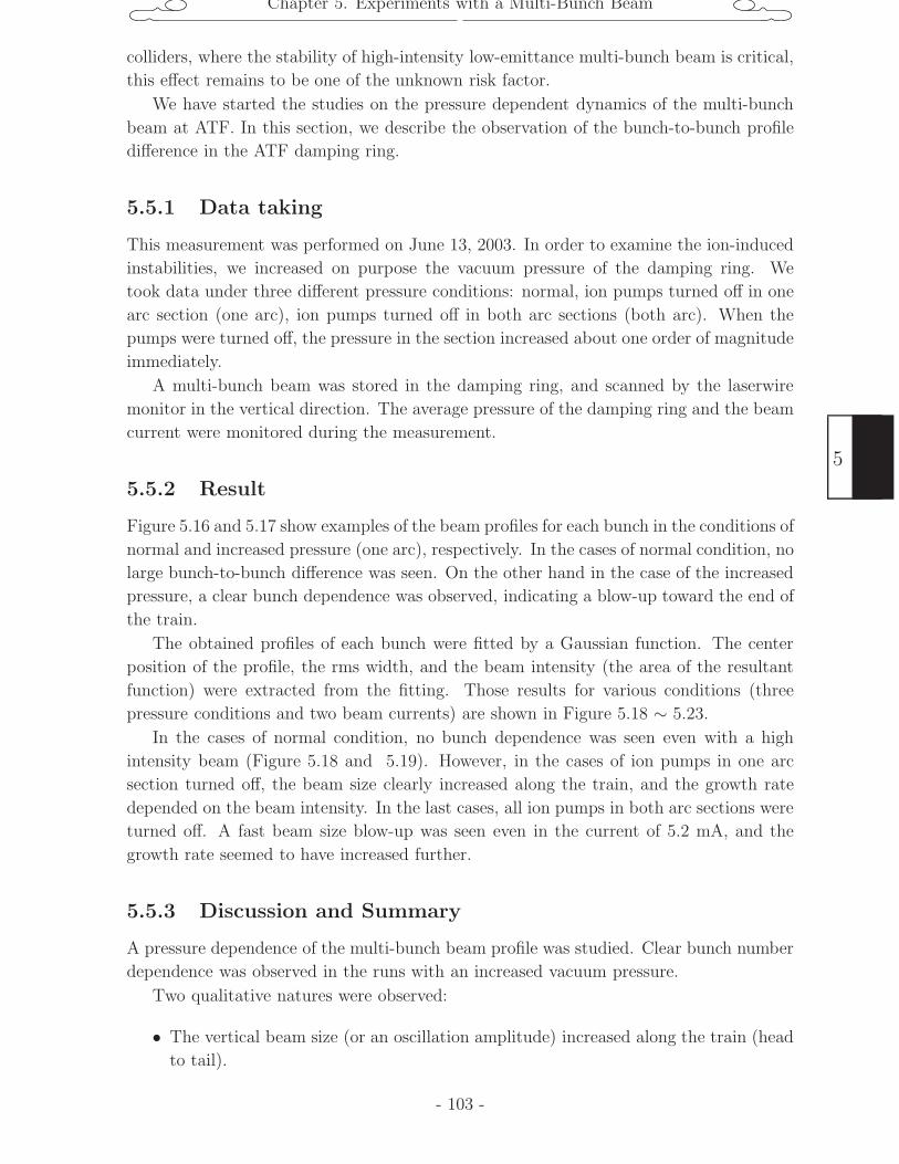
Chapter 5. Experiments with a Multi-Bunch Beam
colliders, where the stability of high-intensity low-emittance multi-bunch beam is critical,
this effect remains to be one of the unknown risk factor.
We have started the studies on the pressure dependent dynamics of the multi-bunch
beam at ATF. In this section, we describe the observation of the bunch-to-bunch profile
difference in the ATF damping ring.
5.5.1 Data taking
This measurement was performed on June 13, 2003. In order to examine the ion-induced
instabilities, we increased on purpose the vacuum pressure of the damping ring. We
took data under three different pressure conditions: normal, ion pumps turned off in one
arc section (one arc), ion pumps turned off in both arc sections (both arc). When the
pumps were turned off, the pressure in the section increased about one order of magnitude
immediately.
A multi-bunch beam was stored in the damping ring, and scanned by the laserwire
monitor in the vertical direction. The average pressure of the damping ring and the beam
current were monitored during the measurement.
5.5.2 Result
Figure 5.16 and 5.17 show examples of the beam profiles for each bunch in the conditions of
normal and increased pressure (one arc), respectively. In the cases of normal condition, no
large bunch-to-bunch difference was seen. On the other hand in the case of the increased
pressure, a clear bunch dependence was observed, indicating a blow-up toward the end of
the train.
The obtained profiles of each bunch were fitted by a Gaussian function. The center
position of the profile, the rms width, and the beam intensity (the area of the resultant
function) were extracted from the fitting. Those results for various conditions (three
pressure conditions and two beam currents) are shown in Figure 5.18 ∼ 5.23.
In the cases of normal condition, no bunch dependence was seen even with a high
intensity beam (Figure 5.18 and 5.19). However, in the cases of ion pumps in one arc
section turned off, the beam size clearly increased along the train, and the growth rate
depended on the beam intensity. In the last cases, all ion pumps in both arc sections were
turned off. A fast beam size blow-up was seen even in the current of 5.2 mA, and the
growth rate seemed to have increased further.
5.5.3 Discussion and Summary
A pressure dependence of the multi-bunch beam profile was studied. Clear bunch number
dependence was observed in the runs with an increased vacuum pressure.
Two qualitative natures were observed:
• The vertical beam size (or an oscillation amplitude) increased along the train (head
to tail).
- 103 -
5
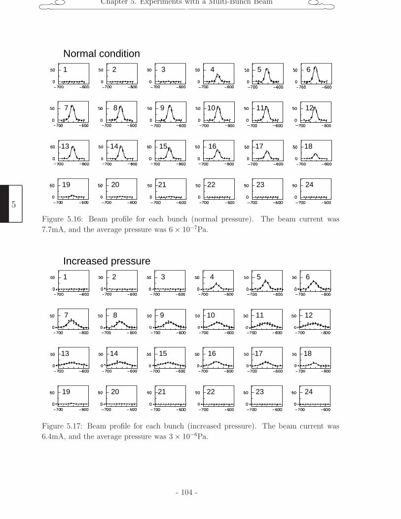
Chapter 5. Experiments with a Multi-Bunch Beam
Normal condition
1 2 3 4 5
9
13 17
21
6
10
14 18
22
7 11
15
19 23
8 12
16
20 24
Figure 5.16: Beam profile for each bunch (normal pressure). The beam current was
7.7mA, and the average pressure was 6 × 10⁻⁷Pa.
Increased pressure
1 2 3 4 5
9
13 17
21
6
10
14 18
22
7 11
15
19 23
8 12
16
20 24
Figure 5.17: Beam profile for each bunch (increased pressure). The beam current was
6.4mA, and the average pressure was 3 × 10⁻⁶Pa.
5
- 104 -
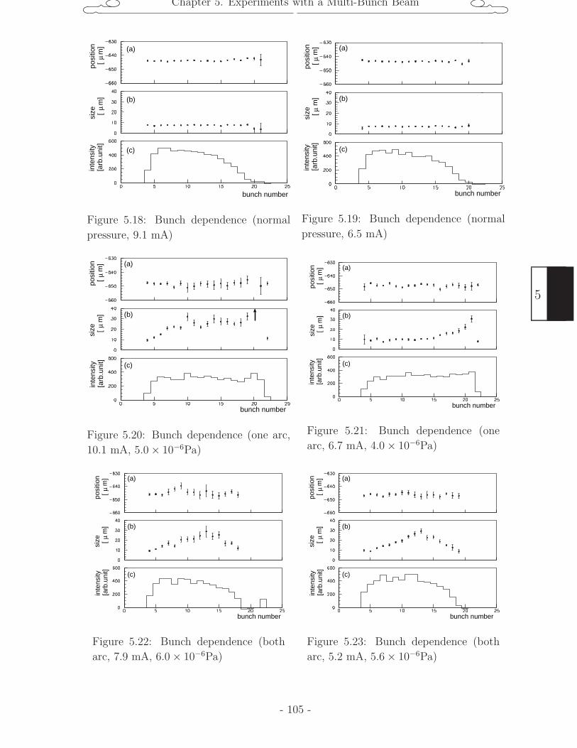
Chapter 5. Experiments with a Multi-Bunch Beam
posi
tion
[
m]
µsi
ze [
m
]µ
inte
nsity
[a
rb.u
nit]
(a)
(b)
(c)
bunch number
Figure 5.18: Bunch dependence (normal
pressure, 9.1 mA)
posi
tion
[
m]
µsi
ze [
m
]µ
inte
nsity
[a
rb.u
nit]
(a)
(b)
(c)
bunch number
Figure 5.19: Bunch dependence (normal
pressure, 6.5 mA)
posi
tion
[
m]
µsi
ze [
m
]µ
inte
nsity
[a
rb.u
nit]
(a)
(b)
(c)
bunch number
Figure 5.20: Bunch dependence (one arc,
10.1 mA, 5.0 × 10⁻⁶Pa)
posi
tion
[
m]
µsi
ze [
m
]µ
inte
nsity
[a
rb.u
nit]
(a)
(b)
(c)
bunch number
Figure 5.21: Bunch dependence (one
arc, 6.7 mA, 4.0 × 10⁻⁶Pa)
posi
tion
[
m]
µsi
ze [
m
]µ
inte
nsity
[a
rb.u
nit]
(a)
(b)
(c)
bunch number
Figure 5.22: Bunch dependence (both
arc, 7.9 mA, 6.0 × 10⁻⁶Pa)
posi
tion
[
m]
µsi
ze [
m
]µ
inte
nsity
[a
rb.u
nit]
(a)
(b)
(c)
bunch number
Figure 5.23: Bunch dependence (both
arc, 5.2 mA, 5.6 × 10⁻⁶Pa)
- 105 -
5
Chapter 5. Experiments with a Multi-Bunch Beam
• The growth rate depends on the beam intensity and the vacuum pressure.
These results agree with the expectation of the fast-beam-ion instability, at least qualita-
tively.
Several improvements will be necessary to make the discussion quantitative. First of
all, the intensity variation in a train should be reduced within a few %. In reality, the
intensity distribution in the train varied in each fill. Stable and efficient injection of the
multi-bunch beam into the damping ring is required. Second, a longitudinal motion of the
bunch was observed by the streak camera. The amplitude of the longitudinal oscillation
was also found to grow along the train. If there was a much larger momentum spread
than those measured under the normal pressure, it would have affected the transverse
motion.
As a final comment in this section, we like to point out the following fact. The
laserwire measures an averaged beam of many revolutions. Thus, a transverse oscillation
of the beam position can imitate an increase in the beam size. With the laserwire monitor
alone, it can not be distinguished whether the measured beam size growth is a real beam
size growth or an increase of a transverse oscillation. In order to measure the transverse
oscillation, a beam position monitor with multi-bunch detection circuits or a spectrum
analysis of a BPM pick-up signal will be useful.5
- 106 -
Chapter 6. Conclusion
Chapter 6
Conclusion
We described the studies of a low emittance electron beam in the ATF damping ring.
ATF is a test accelerator built in KEK. Its goal is to experimentally prove the production
of the low emittance beam required for future linear colliders.
To diagnose its ultra-low emittance beam realized in the damping ring, a unique
instrument called a laserwire beam profile monitor was developed and upgraded. This
monitor works as follows. A thin wire of photon (laserwire) is produced in a Fabry-Perot
optical cavity which is externally excited by a CW laser. The optical cavity is precisely
controlled to keep the resonance condition. By scanning the laserwire across an electron
beam while measuring the flux of the Compton scattering signal rate, a transverse profile
of the electron beam is obtained. The salient feature of this monitor is its reliability and
non-invasiveness of the measurement. Two orthogonal laserwires measure the beam sizes
of two transverse directions. In 2000, the laserwire monitor (horizontal only) was installed
in the north straight section of the ATF damping ring, and made its first successful
measurement of the vertical beam emittance. In 2002, we upgraded the system in several
aspects. We improved its resolution by reducing the laserwire width, and shortened data
acquisition time by increasing the effective intensity of the laserwire. We installed a
vertical laserwire system in addition to the horizontal one. The signal detection scheme
was also modified to separately measure the beam profiles of each bunch in a multi-bunch
train.
Intending to prove the achievement of an ultra-low emittance in the ATF damping ring,
and to understand the mechanism of intensity-dependent emittance growth, we performed
a series of systematic studies. We began the measurement with the single bunch beam.
Actually we measured the four dimensional beam properties, (the transverse emittances,
bunch length, and momentum spread), and their intensity dependence under various ring
conditions. Our main conclusion from the study are as follows. In the case of a well-
tuned condition, the vertical emittance was found to reach as small as 4 pm·rad in the
zero current limit, and grow by about factor 1.5 at the intensity of 1010. The result proved
that a low emittance beam required for the linear colliders has been produced at least in
the single bunch mode. As to the intensity dependence, all observed quantities showed,
more or less, such dependences. First of all, the momentum spread was found to show
an intensity dependence, but its strength (the slope of the intensity dependence) became
- 107 -
6
Chapter 6. Conclusion
weaker as the vertical emittance was enlarged. Second, both horizontal and vertical
emittances showed intensity dependences; their strength were similar in magnitude. The
bunch length was also found to depend on the beam intensity, but the slope seemed to be
independent of the bunch volume. The bunch lengthening can be understood naively by
the effect of the wake field. On the other hand, the emittances and momentum spread are
determined by the intra-beam scattering. In order to understand the mechanism of these
intensity dependences, we developed a beam simulation code. Actually, the SAD code
was modified to include the effect of longitudinal wake field in addition to the intra-beam
scattering. The impedance of the beam line was estimated from the bunch lengthening.
The overall nature of the emittance, bunch length and momentum spread under the
various conditions of the ring tuning seems to have no serious disagreement with this
model calculation.
In the multi-bunch operational mode, a train with 20-bunches spaced 2.8 nsec interval
was filled in the damping ring. The transverse emittances of each bunch were diagnosed
by the laserwire monitor. It proved that a similar small emittance as the single bunch
mode was realized even in the multi-bunch mode. No large bunch-to-bunch differences
were seen. Although the bunch intensity of the stored beam was still much lower than our
target, the observation is a promising milestone toward the goal. To investigate the effect
of instabilities caused by the ions in the beam, vacuum pressure dependence of the beam
size was studied. A clear beam blow-up along the train was seen under the condition of
an increased pressure, suggesting the fast-beam-ion instability. This effect may limit the
performance of the vertical emittance of the multi-bunch mode in a high intensity region.
The attained transverse emittances are plotted in Figure 6.1 with our target. Although
the horizontal emittance is determined from the ring design, the vertical emittance can
be reduced by the precise alignment and/or the beam tuning. It shows that we succeeded
in reducing the vertical emittance to a half of the initial target value and reached the
requirement of GLC at the design bunch intensity. In the multi-bunch mode, the vertical
emittance reached our initial design in run 1. And was further reduced later, in run 2 at
a lower intensity. We hope we can satisfy the GLC requirement even in the multi-bunch
mode with the design intensity.
Basically the main study goal in the ATF damping ring, the low-emittance beam
production, has been achieved successfully. In the future, the first to be proved in ATF
should be the production of a required emittance with a high current (design bunch
intensity) in the multi-bunch mode. Stable and efficient injection to (and extraction
from) the damping ring have to be realized. Energy compensation in the linac have
to be tuned to stabilize the multi-bunch injection. The extraction kicker system needs
some modifications to extract all bunches in the train in the same orbit. The emittance
measurement should be performed in the extraction line. The multi-bunch instabilities
in the ring have to be studied by the laserwire and other instruments. The future linear
colliders require further reduction in the damping time to achieve a high repetition rate
and thus a high luminosity. This can be achieved with wiggler magnets in the ring; the
role of these magnets is to shorten the damping time by additional synchrotron radiation.
In the experiments presented in this theses, the wiggler magnets were being installed but
6
- 108 -
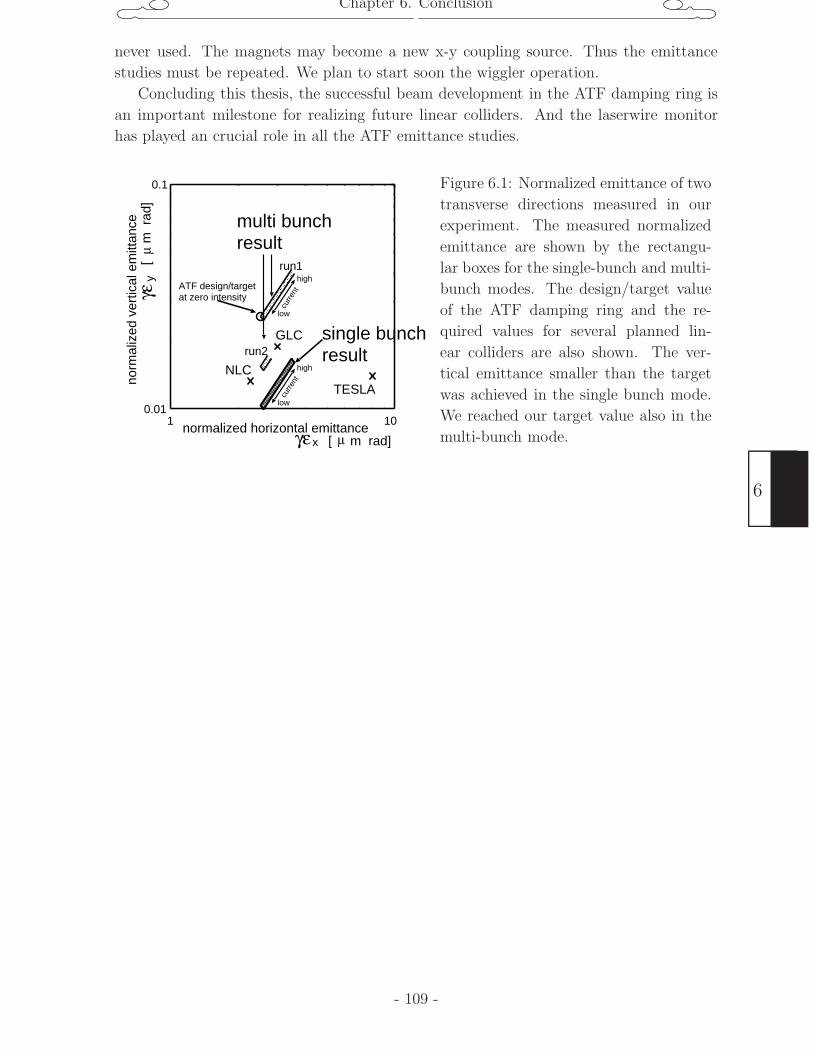
Chapter 6. Conclusion
never used. The magnets may become a new x-y coupling source. Thus the emittance
studies must be repeated. We plan to start soon the wiggler operation.
Concluding this thesis, the successful beam development in the ATF damping ring is
an important milestone for realizing future linear colliders. And the laserwire monitor
has played an crucial role in all the ATF emittance studies.
γε
γεy
x
[
m r
ad]
[ m rad]µ
µno
rmal
ized
ver
tical
em
ittan
ce
normalized horizontal emittance
0.1
0.011 10
ATF design/targetat zero intensity
single bunchresult
GLC
TESLA
multi bunchresult
high
low
curre
nt
high
low
curre
nt
NLC
run1
run2
Figure 6.1: Normalized emittance of two
transverse directions measured in our
experiment. The measured normalized
emittance are shown by the rectangu-
lar boxes for the single-bunch and multi-
bunch modes. The design/target value
of the ATF damping ring and the re-
quired values for several planned lin-
ear colliders are also shown. The ver-
tical emittance smaller than the target
was achieved in the single bunch mode.
We reached our target value also in the
multi-bunch mode.
- 109 -
6
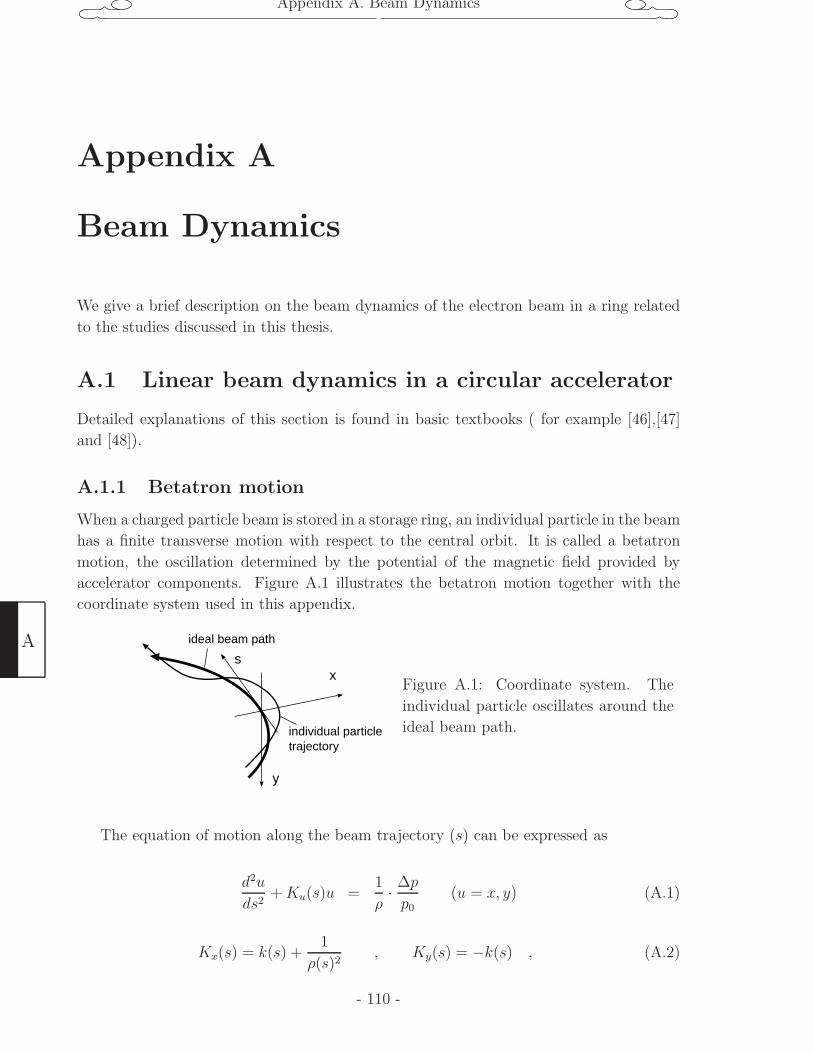
Appendix A. Beam Dynamics
Appendix A
Beam Dynamics
We give a brief description on the beam dynamics of the electron beam in a ring related
to the studies discussed in this thesis.
A.1 Linear beam dynamics in a circular accelerator
Detailed explanations of this section is found in basic textbooks ( for example [46],[47]
and [48]).
A.1.1 Betatron motion
When a charged particle beam is stored in a storage ring, an individual particle in the beam
has a finite transverse motion with respect to the central orbit. It is called a betatron
motion, the oscillation determined by the potential of the magnetic field provided by
accelerator components. Figure A.1 illustrates the betatron motion together with the
coordinate system used in this appendix.
x
y
s
individual particletrajectory
ideal beam path
Figure A.1: Coordinate system. The
individual particle oscillates around the
ideal beam path.
The equation of motion along the beam trajectory (s) can be expressed as
d2u
ds2+Ku(s)u =
1
ρ· ∆p
p0(u = x, y) (A.1)
Kx(s) = k(s) +1
ρ(s)2, Ky(s) = −k(s) , (A.2)
A
- 110 -
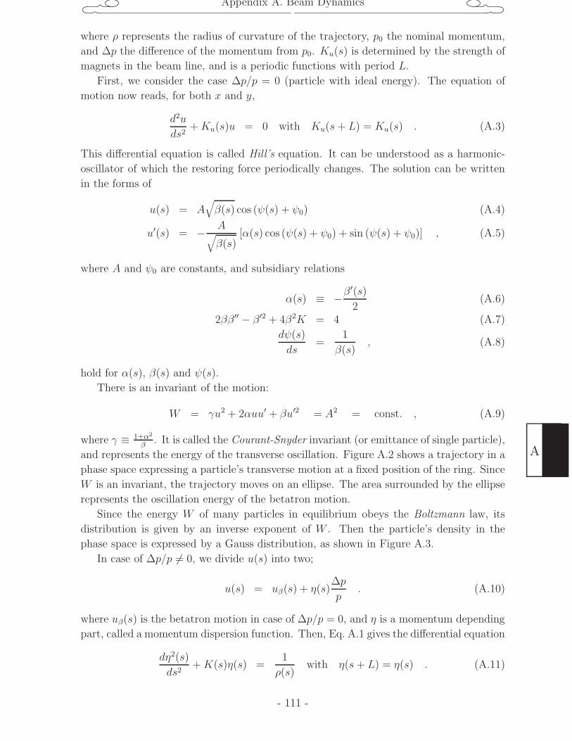
Appendix A. Beam Dynamics
where ρ represents the radius of curvature of the trajectory, p0 the nominal momentum,
and ∆p the difference of the momentum from p0. Ku(s) is determined by the strength of
magnets in the beam line, and is a periodic functions with period L.
First, we consider the case ∆p/p = 0 (particle with ideal energy). The equation of
motion now reads, for both x and y,
d2u
ds2+Ku(s)u = 0 with Ku(s+ L) = Ku(s) . (A.3)
This differential equation is called Hill’s equation. It can be understood as a harmonic-
oscillator of which the restoring force periodically changes. The solution can be written
in the forms of
u(s) = A√β(s) cos (ψ(s) + ψ0) (A.4)
u′(s) = − A√β(s)
[α(s) cos (ψ(s) + ψ0) + sin (ψ(s) + ψ0)] , (A.5)
where A and ψ0 are constants, and subsidiary relations
α(s) ≡ −β′(s)2
(A.6)
2ββ ′′ − β ′2 + 4β2K = 4 (A.7)
dψ(s)
ds=
1
β(s), (A.8)
hold for α(s), β(s) and ψ(s).
There is an invariant of the motion:
W = γu2 + 2αuu′ + βu′2 = A2 = const. , (A.9)
where γ ≡ 1+α2
β. It is called the Courant-Snyder invariant (or emittance of single particle),
and represents the energy of the transverse oscillation. Figure A.2 shows a trajectory in a
phase space expressing a particle’s transverse motion at a fixed position of the ring. Since
W is an invariant, the trajectory moves on an ellipse. The area surrounded by the ellipse
represents the oscillation energy of the betatron motion.
Since the energy W of many particles in equilibrium obeys the Boltzmann law, its
distribution is given by an inverse exponent of W . Then the particle’s density in the
phase space is expressed by a Gauss distribution, as shown in Figure A.3.
In case of ∆p/p = 0, we divide u(s) into two;
u(s) = uβ(s) + η(s)∆p
p. (A.10)
where uβ(s) is the betatron motion in case of ∆p/p = 0, and η is a momentum depending
part, called a momentum dispersion function. Then, Eq. A.1 gives the differential equation
dη2(s)
ds2+K(s)η(s) =
1
ρ(s)with η(s+ L) = η(s) . (A.11)
- 111 -
A
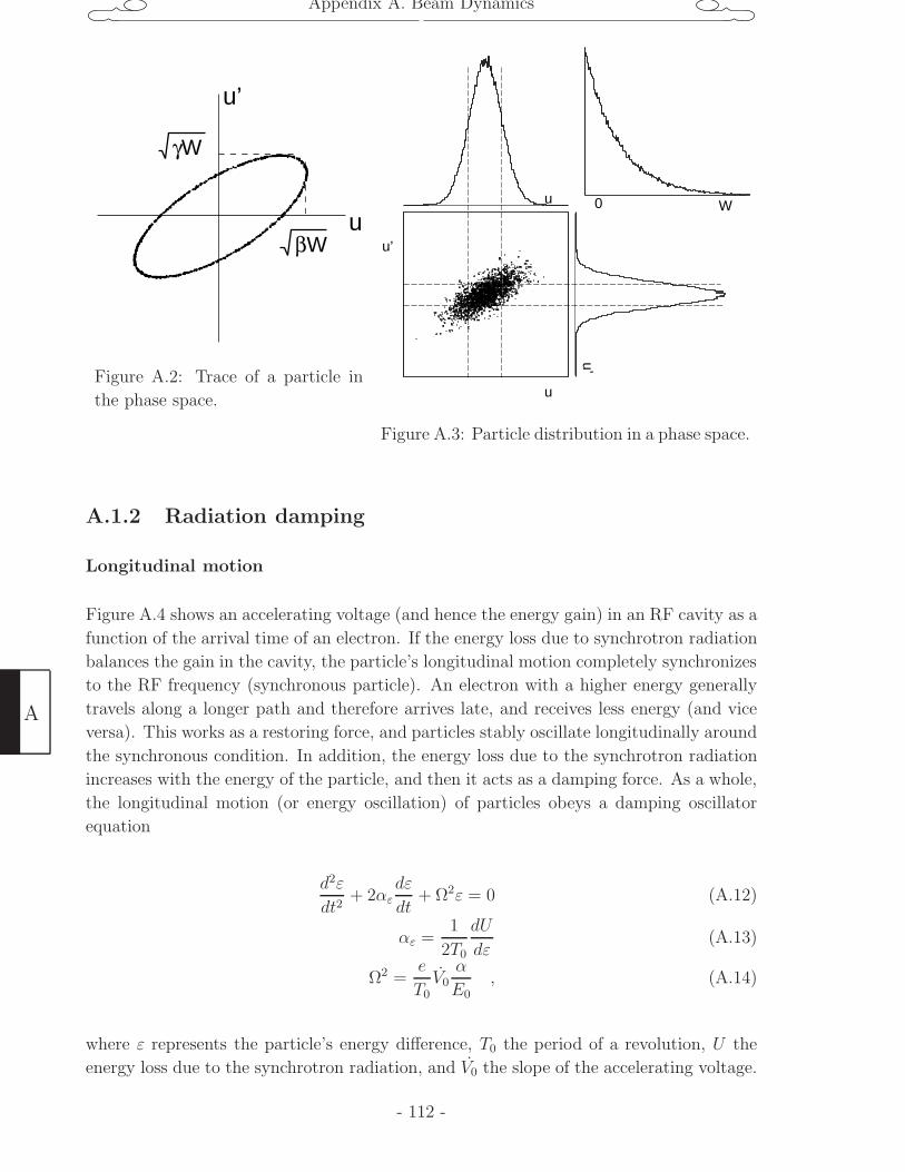
Appendix A. Beam Dynamics
u
u’
γW
βW
Figure A.2: Trace of a particle in
the phase space.
W
u
u’
u’
u 0
Figure A.3: Particle distribution in a phase space.
A.1.2 Radiation damping
Longitudinal motion
Figure A.4 shows an accelerating voltage (and hence the energy gain) in an RF cavity as a
function of the arrival time of an electron. If the energy loss due to synchrotron radiation
balances the gain in the cavity, the particle’s longitudinal motion completely synchronizes
to the RF frequency (synchronous particle). An electron with a higher energy generally
travels along a longer path and therefore arrives late, and receives less energy (and vice
versa). This works as a restoring force, and particles stably oscillate longitudinally around
the synchronous condition. In addition, the energy loss due to the synchrotron radiation
increases with the energy of the particle, and then it acts as a damping force. As a whole,
the longitudinal motion (or energy oscillation) of particles obeys a damping oscillator
equation
d2ε
dt2+ 2αε
dε
dt+ Ω2ε = 0 (A.12)
αε =1
2T0
dU
dε(A.13)
Ω2 =e
T0V0
α
E0, (A.14)
where ε represents the particle’s energy difference, T0 the period of a revolution, U the
energy loss due to the synchrotron radiation, and V0 the slope of the accelerating voltage.
A
- 112 -
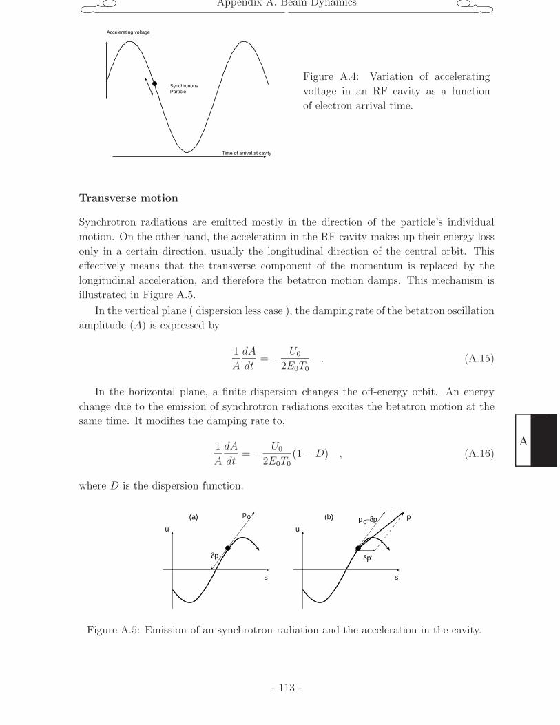
Appendix A. Beam Dynamics
Time of arrival at cavity
Accelerating voltage
SynchronousParticle
Figure A.4: Variation of accelerating
voltage in an RF cavity as a function
of electron arrival time.
Transverse motion
Synchrotron radiations are emitted mostly in the direction of the particle’s individual
motion. On the other hand, the acceleration in the RF cavity makes up their energy loss
only in a certain direction, usually the longitudinal direction of the central orbit. This
effectively means that the transverse component of the momentum is replaced by the
longitudinal acceleration, and therefore the betatron motion damps. This mechanism is
illustrated in Figure A.5.
In the vertical plane ( dispersion less case ), the damping rate of the betatron oscillation
amplitude (A) is expressed by
1
A
dA
dt= − U0
2E0T0. (A.15)
In the horizontal plane, a finite dispersion changes the off-energy orbit. An energy
change due to the emission of synchrotron radiations excites the betatron motion at the
same time. It modifies the damping rate to,
1
A
dA
dt= − U0
2E0T0(1 −D) , (A.16)
where D is the dispersion function.
u
s
p
δp
u
s
p
δp
(a) (b)0
0
’
−δp p
Figure A.5: Emission of an synchrotron radiation and the acceleration in the cavity.
- 113 -
A

Appendix A. Beam Dynamics
A.1.3 Quantum excitation and equilibrium
Quantum excitation
Actual energy loss due to the synchrotron radiation occurs in a discrete energy unit of a
photon. It introduces a kind of noise, resulting in a growth of the oscillation amplitude.
The growth rate of the energy spread is given
∆
(∆p
p
)2
=2re
3Cqγ
5∮
1
|ρ3|ds , (A.17)
where Cq = 5532
√3
hmc
. It is converted into the energy change of the transverse motion (∆W )
via the dispersion
∆W = (γη2 + 2αηη′ + βη′2)
(∆p
p
)2
≡ H(s)
(∆p
p
)2
. (A.18)
Equilibrium
The equilibrium of the energy spread and transverse emittances are determined by the
balance of the radiation damping and the quantum excitation. They are;
(σp
p
)2
= Cqγ2
Jε
∮ 1|ρ3|ds∮ 1ρ2ds
and εx = Cqγ2
Jx
∮ H|ρ3|ds∮ 1ρ2ds
, (A.19)
where Jε and Jx are the damping partition numbers for longitudinal and horizontal di-
rection, respectively. The bunch length is related to the energy spread by
στ =α
ΩE0σε . (A.20)
Vertical emittance
Since there is no bending in the vertical plane, the vertical emittance is not determined
from the design of the beam-optics. In practice, it is governed mainly by:
• vertical dispersion errors, arising from vertical bending fields produced by position-
ing errors of the magnets.
• coupling of the horizontal and vertical betatron motion, arising from skew-quadrupole
field errors. It is produced by angular positioning errors of the quadrupoles and also
by vertical closed orbit errors in sextupole magnets.
The coupling is usually expressed by a constant κ which describes the sharing of the
natural emittance ε0 between two planes;
εx =1
1 + κε0 , εy =
κ
1 + κε0 . (A.21)
A
- 114 -
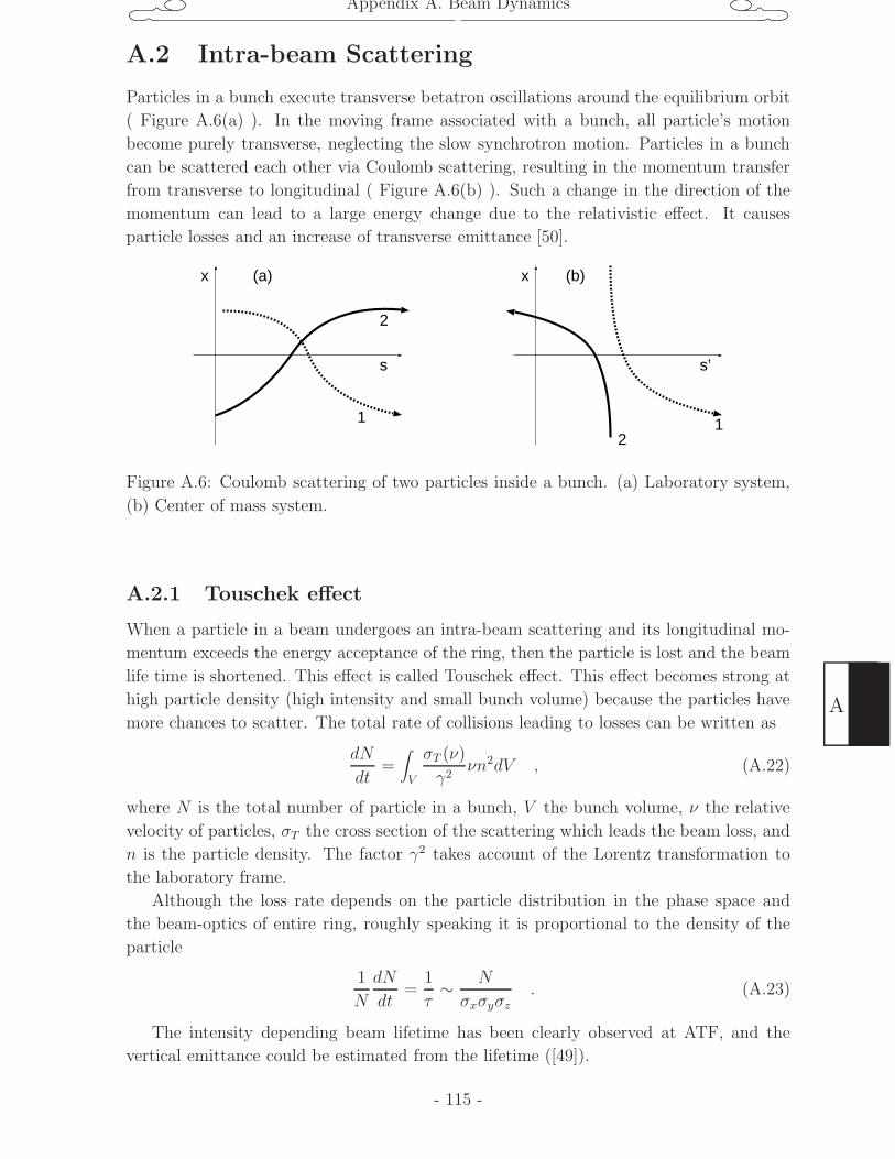
Appendix A. Beam Dynamics
A.2 Intra-beam Scattering
Particles in a bunch execute transverse betatron oscillations around the equilibrium orbit
( Figure A.6(a) ). In the moving frame associated with a bunch, all particle’s motion
become purely transverse, neglecting the slow synchrotron motion. Particles in a bunch
can be scattered each other via Coulomb scattering, resulting in the momentum transfer
from transverse to longitudinal ( Figure A.6(b) ). Such a change in the direction of the
momentum can lead to a large energy change due to the relativistic effect. It causes
particle losses and an increase of transverse emittance [50].
(a) (b)
s
x x
s’
2
12
1
Figure A.6: Coulomb scattering of two particles inside a bunch. (a) Laboratory system,
(b) Center of mass system.
A.2.1 Touschek effect
When a particle in a beam undergoes an intra-beam scattering and its longitudinal mo-
mentum exceeds the energy acceptance of the ring, then the particle is lost and the beam
life time is shortened. This effect is called Touschek effect. This effect becomes strong at
high particle density (high intensity and small bunch volume) because the particles have
more chances to scatter. The total rate of collisions leading to losses can be written as
dN
dt=∫
V
σT (ν)
γ2νn2dV , (A.22)
where N is the total number of particle in a bunch, V the bunch volume, ν the relative
velocity of particles, σT the cross section of the scattering which leads the beam loss, and
n is the particle density. The factor γ2 takes account of the Lorentz transformation to
the laboratory frame.
Although the loss rate depends on the particle distribution in the phase space and
the beam-optics of entire ring, roughly speaking it is proportional to the density of the
particle
1
N
dN
dt=
1
τ∼ N
σxσyσz. (A.23)
The intensity depending beam lifetime has been clearly observed at ATF, and the
vertical emittance could be estimated from the lifetime ([49]).
- 115 -
A
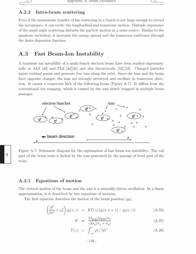
Appendix A. Beam Dynamics
A.2.2 Intra-beam scattering
Even if the momentum transfer of the scattering in a bunch is not large enough to exceed
the acceptance, it can excite the longitudinal and transverse motion. Multiple experience
of the small angle scattering disturbs the particle motion as a noise source. Similar to the
quantum excitation, it increases the energy spread and the transverse emittance through
the finite dispersion function.
A.3 Fast Beam-Ion Instability
A transient ion instability of a multi-bunch electron beam have been studied experimen-
tally at ALS [43] and PLS [44][45] and also theoretically [52],[53]. Charged particles
ionize residual gasses and generate free ions along the orbit. Since the ions and the beam
have opposite charges, the ions are strongly attracted and oscillate in transverse direc-
tion. It causes a transverse kick of the following beam (Figure A.7). It differs from the
conventional ion trapping, which is caused by the ions slowly trapped in multiple beam
passages.
e-e-
e-e-
e-
e-
e-+ + +
++
+
+
+
+
+++
+
+ ++
+
+++
++
+
+
+
++
+
s
ionselectron bunches
zbeam direction
Figure A.7: Schematic diagram for the explanation of fast beam ion instability. The tail
part of the beam train is kicked by the ions generated by the passage of head part of the
train.
A.3.1 Equations of motion
The vertical motion of the beam and the ions is a mutually-driven oscillation. In a linear
approximation, it is described by two equations of motions.
The first equation describes the motion of the beam position (yb),
(d2
ds2+ ω2
β
)yb(s, z) = KΓ(z) (yi(s, s+ z) − yb(s, z)) (A.24)
K ≈ 4λion(pgas)re
γ3σy(σx + σy)(A.25)
Γ(z) =∫ z
−∞ρ(z′)dz′ . (A.26)
A
- 116 -
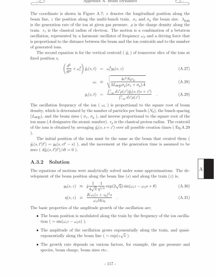
Appendix A. Beam Dynamics
The coordinate is shown in Figure A.7; s denotes the longitudinal position along the
beam line, z the position along the multi-bunch train. σx and σy the beam size. λionis the generation rate of the ion at given gas pressure. ρ is the charge density along the
train. re is the classical radius of electron. The motion is a combination of a betatron
oscillation, represented by a harmonic oscillator of frequency ωβ and a driving force that
is proportional to the distance between the beam and the ion centroids and to the number
of generated ions.
The second equation is for the vertical centroid ( yi ) of transverse slice of the ions at
fixed position s, (d2
dt2+ ω2
i
)yi(s, t) = ω2
i yb(s, z) (A.27)
ωi ≡√√√√ 4c2Nbrp
3Lsepσy(σx + σy)A(A.28)
yi(s, t) =
∫ z−∞ dz′ρ(z′)yi(s, t|s+ z′)∫ z
−∞ dz′ρ(z′). (A.29)
The oscillation frequency of the ion ( ωi ) is proportional to the square root of beam
density, which is determined by the number of particles per bunch (Nb), the bunch spacing
(Lsep), and the beam sizes ( σx, σy ), and inverse proportional to the square root of the
ion mass (A designates the atomic number). rp is the classical proton radius. The centroid
of the ions is obtained by averaging yi(s, s+ z′) over all possible creation times ( Eq.A.29
).
The initial position of the ions must be the same as the beam that created them (
yi(s, t′|t′) = yb(s, ct
′ − s) ), and the movement at the generation time is assumed to be
zero ( dyi(s, t′|t′)/dt = 0 ).
A.3.2 Solution
The equations of motions were analytically solved under some approximations. The de-
velopment of the beam position along the beam line (s) and along the train (z) is,
yb(s, z) ≈ y1
4√π
1
η1/4exp(2
√η) sin(ωiz − ωβs+ θ) (A.30)
η(s, z) ≡ Kωi(z + z0)2s
ωβ16z0. (A.31)
The basic properties of the amplitude growth of the oscillation are;
• The beam position is modulated along the train by the frequency of the ion oscilla-
tion ( ∼ sin(ωiz − ωβs) ).
• The amplitude of the oscillation grows exponentially along the train, and quasi-
exponentially along the beam line ( ∼ exp(z√s ).
• The growth rate depends on various factors, for example, the gas pressure and
species, beam charge, beam sizes etc..
- 117 -
A
Appendix B. Laserwire Monitor Utilizing a Higher Order Mode
Appendix B
Laserwire Monitor Utilizing a
Higher Order Mode
As explained in Chapter 4, ATF succeeded in reducing the vertical emittance to the half
of its original target value. Such a small beam size close to the resolution limit of the
present laserwire monitor. For example, we measured an electron beam of 4 µm with a
laserwire of 5.6 µm, and obtained a count rate profile of 6.9 µm as a convolution. The
laserwire was thicker than the beam size. Apparently, it is not possible to measure much
smaller beam size by the present setup.
In order to improve the resolution of the laserwire, it has been proposed to use a
higher order mode of the Gaussian beam. In this chapter, we describe the method and
the results of the first experiment done with this new technique.
B.1 An idea of utilizing the higher order mode
B.1.1 Diffraction limit
A laser beam has a parabolic shape along its longitudinal axis. The length of the central
part is characterized by the Rayleigh length (z0), and z0 is determined by w0 and λ
(Eq.3.39). If we design a beam waist to be smaller, the Rayleigh length also becomes
smaller.
In the case of ATF, the electron beam has a flat shape with an aspect ratio of about
10:1. We must be careful in choosing the Rayleigh length not too small compared to the
horizontal size of the electron beam. In fact, if the beam waist (w0) is reduced to less
than 10 µm, the laser beam can not be treated as a simple solid wire which has a constant
width. This situation is illustrated in Figure B.1.
To avoid this effect, the only way is to change the laser wave length. However, there
are some technical problems in using shorter wave length. Fabrication of a low-loss and
high-reflectance mirror suit for a high finesse cavity is quite difficult in the short wave
length region. A high power and stable laser which meets our specification is also not
available now. We conclude that the diffraction effect and some technical difficulties limit
the resolution of the current laserwire monitor.
B
- 118 -
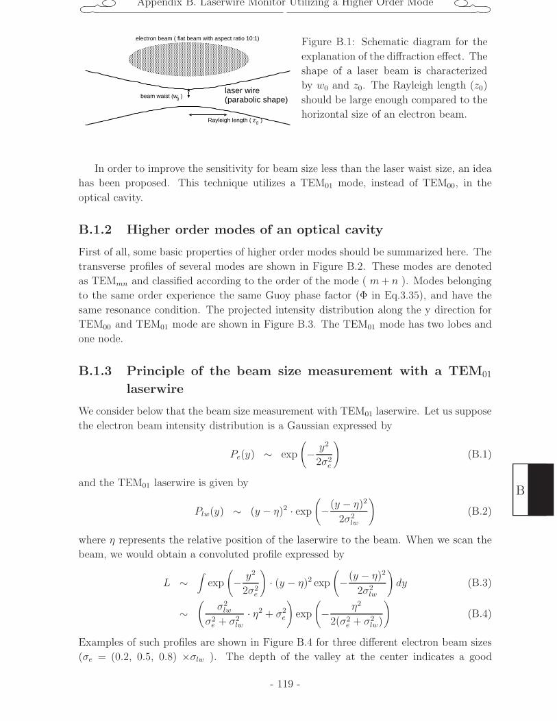
Appendix B. Laserwire Monitor Utilizing a Higher Order Mode
Rayleigh length ( z )0
electron beam ( flat beam with aspect ratio 10:1)
laser wire(parabolic shape)beam waist (w )0
Figure B.1: Schematic diagram for the
explanation of the diffraction effect. The
shape of a laser beam is characterized
by w0 and z0. The Rayleigh length (z0)
should be large enough compared to the
horizontal size of an electron beam.
In order to improve the sensitivity for beam size less than the laser waist size, an idea
has been proposed. This technique utilizes a TEM01 mode, instead of TEM00, in the
optical cavity.
B.1.2 Higher order modes of an optical cavity
First of all, some basic properties of higher order modes should be summarized here. The
transverse profiles of several modes are shown in Figure B.2. These modes are denoted
as TEMmn and classified according to the order of the mode ( m+ n ). Modes belonging
to the same order experience the same Guoy phase factor (Φ in Eq.3.35), and have the
same resonance condition. The projected intensity distribution along the y direction for
TEM00 and TEM01 mode are shown in Figure B.3. The TEM01 mode has two lobes and
one node.
B.1.3 Principle of the beam size measurement with a TEM01
laserwire
We consider below that the beam size measurement with TEM01 laserwire. Let us suppose
the electron beam intensity distribution is a Gaussian expressed by
Pe(y) ∼ exp
(− y2
2σ2e
)(B.1)
and the TEM01 laserwire is given by
Plw(y) ∼ (y − η)2 · exp
(−(y − η)2
2σ2lw
)(B.2)
where η represents the relative position of the laserwire to the beam. When we scan the
beam, we would obtain a convoluted profile expressed by
L ∼∫
exp
(− y2
2σ2e
)· (y − η)2 exp
(−(y − η)2
2σ2lw
)dy (B.3)
∼(
σ2lw
σ2e + σ2
lw
· η2 + σ2e
)exp
(− η2
2(σ2e + σ2
lw)
)(B.4)
Examples of such profiles are shown in Figure B.4 for three different electron beam sizes
(σe = (0.2, 0.5, 0.8) ×σlw ). The depth of the valley at the center indicates a good
- 119 -
B
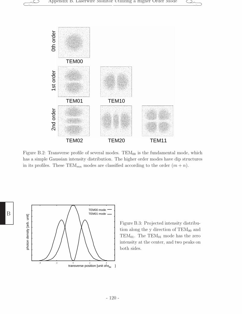
Appendix B. Laserwire Monitor Utilizing a Higher Order Mode
0th
orde
r1s
t ord
er2n
d or
der
TEM00
TEM01
TEM02
TEM10
TEM20 TEM11
Figure B.2: Transverse profile of several modes. TEM00 is the fundamental mode, which
has a simple Gaussian intensity distribution. The higher order modes have dip structures
in its profiles. These TEMmn modes are classified according to the order (m+ n).
-4 -2 0 2 4
TEM00 modeTEM01 mode
transverse position [unit of ]σlw
phot
on d
ensi
ty [a
rb. u
nit]
Figure B.3: Projected intensity distribu-
tion along the y direction of TEM00 and
TEM01. The TEM01 mode has the zero
intensity at the center, and two peaks on
both sides.
B
- 120 -
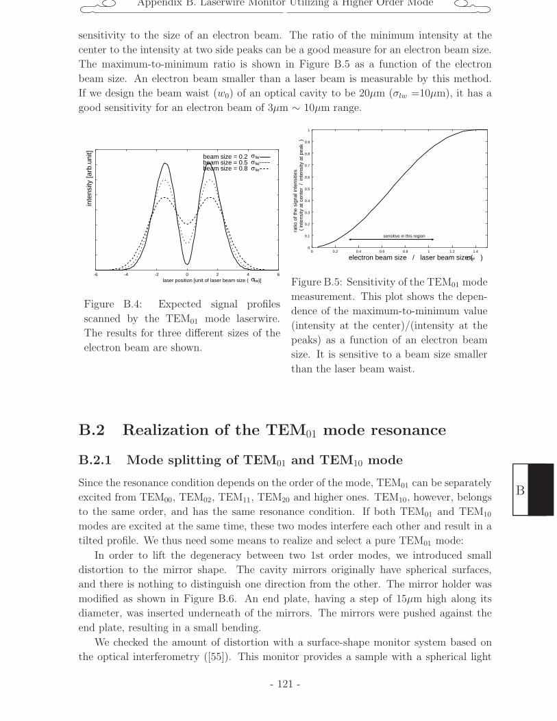
Appendix B. Laserwire Monitor Utilizing a Higher Order Mode
sensitivity to the size of an electron beam. The ratio of the minimum intensity at the
center to the intensity at two side peaks can be a good measure for an electron beam size.
The maximum-to-minimum ratio is shown in Figure B.5 as a function of the electron
beam size. An electron beam smaller than a laser beam is measurable by this method.
If we design the beam waist (w0) of an optical cavity to be 20µm (σlw =10µm), it has a
good sensitivity for an electron beam of 3µm ∼ 10µm range.
-6 -4 -2 0 2 4 6
beam size = 0.2 beam size = 0.5 beam size = 0.8
σσσ
inte
nsity
[arb
.uni
t]
laser position [unit of laser beam size ( )]σlw
lwlwlw
Figure B.4: Expected signal profiles
scanned by the TEM01 mode laserwire.
The results for three different sizes of the
electron beam are shown.
0
0.1
0.2
0.3
0.4
0.5
0.6
0.7
0.8
0.9
1
0 0.2 0.4 0.6 0.8 1 1.2 1.4
electron beam size / laser beam size ( )σlw
ratio
of t
he s
igna
l int
ensi
ties
( in
tens
ity a
t cen
ter
/ in
tens
ity a
t pea
k )
sensitive in this region
Figure B.5: Sensitivity of the TEM01 mode
measurement. This plot shows the depen-
dence of the maximum-to-minimum value
(intensity at the center)/(intensity at the
peaks) as a function of an electron beam
size. It is sensitive to a beam size smaller
than the laser beam waist.
B.2 Realization of the TEM01 mode resonance
B.2.1 Mode splitting of TEM01 and TEM10 mode
Since the resonance condition depends on the order of the mode, TEM01 can be separately
excited from TEM00, TEM02, TEM11, TEM20 and higher ones. TEM10, however, belongs
to the same order, and has the same resonance condition. If both TEM01 and TEM10
modes are excited at the same time, these two modes interfere each other and result in a
tilted profile. We thus need some means to realize and select a pure TEM01 mode:
In order to lift the degeneracy between two 1st order modes, we introduced small
distortion to the mirror shape. The cavity mirrors originally have spherical surfaces,
and there is nothing to distinguish one direction from the other. The mirror holder was
modified as shown in Figure B.6. An end plate, having a step of 15µm high along its
diameter, was inserted underneath of the mirrors. The mirrors were pushed against the
end plate, resulting in a small bending.
We checked the amount of distortion with a surface-shape monitor system based on
the optical interferometry ([55]). This monitor provides a sample with a spherical light
- 121 -
B
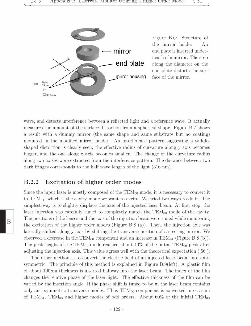
Appendix B. Laserwire Monitor Utilizing a Higher Order Mode
y
x
end plate
mirror
mirror housingstep hight
15µm
width 1mm
Figure B.6: Structure of
the mirror holder. An
end plate is inserted under-
neath of a mirror. The step
along the diameter on the
end plate distorts the sur-
face of the mirror.
wave, and detects interference between a reflected light and a reference wave. It actually
measures the amount of the surface distortion from a spherical shape. Figure B.7 shows
a result with a dummy mirror (the same shape and same substrate but no coating)
mounted in the modified mirror holder. An interference pattern suggesting a saddle-
shaped distortion is clearly seen; the effective radius of curvature along y axis becomes
bigger, and the one along x axis becomes smaller. The change of the curvature radius
along two axises were extracted from the interference pattern. The distance between two
dark fringes corresponds to the half wave length of the light (316 nm).
B.2.2 Excitation of higher order modes
Since the input laser is mostly composed of the TEM00 mode, it is necessary to convert it
to TEM01, which is the cavity mode we want to excite. We tried two ways to do it. The
simplest way is to slightly displace the axis of the injected laser beam. At first step, the
laser injection was carefully tuned to completely match the TEM00 mode of the cavity.
The positions of the lenses and the axis of the injection beam were tuned while monitoring
the excitation of the higher order modes (Figure B.8 (a)). Then, the injection axis was
laterally shifted along y axis by shifting the transverse position of a steering mirror. We
observed a decrease in the TEM00 component and an increase in TEM01 (Figure B.8 (b)).
The peak height of the TEM01 mode reached about 40% of the initial TEM00 peak after
adjusting the injection axis. This value agrees well with the theoretical expectation ([56]).
The other method is to convert the electric field of an injected laser beam into anti-
symmetric. The principle of this method is explained in Figure B.9(left). A plastic film
of about 100µm thickness is inserted halfway into the laser beam. The index of the film
changes the relative phase of the laser light. The effective thickness of the film can be
varied by the insertion angle. If the phase shift is tuned to be π, the laser beam contains
only anti-symmetric transverse modes. Thus TEM00 component is converted into a sum
of TEM01, TEM03 and higher modes of odd orders. About 60% of the initial TEM00
B
- 122 -
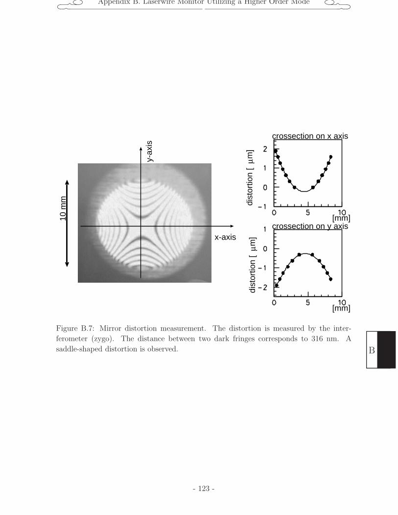
Appendix B. Laserwire Monitor Utilizing a Higher Order Mode
10 m
m
crossection on x axis
y-ax
is
x-axis
dist
ortio
n [
m]
µdi
stor
tion
[ m
]µ
crossection on y axis[mm]
[mm]
Figure B.7: Mirror distortion measurement. The distortion is measured by the inter-
ferometer (zygo). The distance between two dark fringes corresponds to 316 nm. A
saddle-shaped distortion is observed.
- 123 -
B
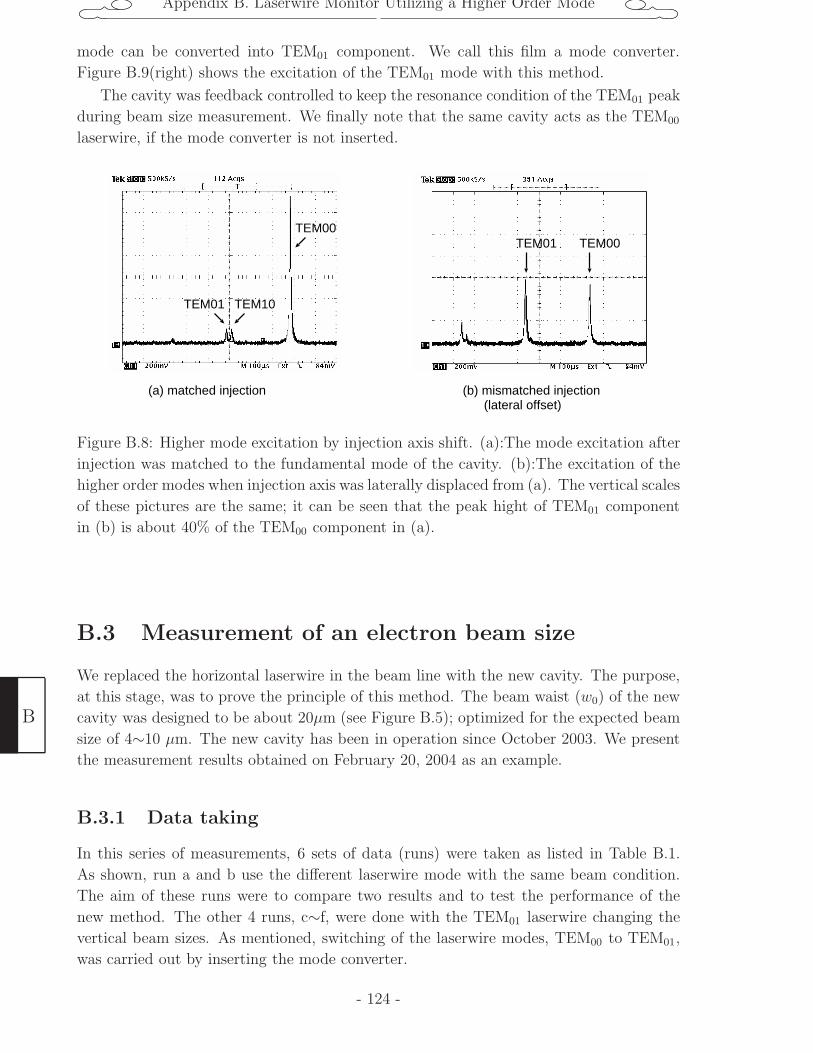
Appendix B. Laserwire Monitor Utilizing a Higher Order Mode
mode can be converted into TEM01 component. We call this film a mode converter.
Figure B.9(right) shows the excitation of the TEM01 mode with this method.
The cavity was feedback controlled to keep the resonance condition of the TEM01 peak
during beam size measurement. We finally note that the same cavity acts as the TEM00
laserwire, if the mode converter is not inserted.
TEM00TEM01TEM00
TEM10TEM01
(a) matched injection (b) mismatched injection (lateral offset)
Figure B.8: Higher mode excitation by injection axis shift. (a):The mode excitation after
injection was matched to the fundamental mode of the cavity. (b):The excitation of the
higher order modes when injection axis was laterally displaced from (a). The vertical scales
of these pictures are the same; it can be seen that the peak hight of TEM01 component
in (b) is about 40% of the TEM00 component in (a).
B.3 Measurement of an electron beam size
We replaced the horizontal laserwire in the beam line with the new cavity. The purpose,
at this stage, was to prove the principle of this method. The beam waist (w0) of the new
cavity was designed to be about 20µm (see Figure B.5); optimized for the expected beam
size of 4∼10 µm. The new cavity has been in operation since October 2003. We present
the measurement results obtained on February 20, 2004 as an example.
B.3.1 Data taking
In this series of measurements, 6 sets of data (runs) were taken as listed in Table B.1.
As shown, run a and b use the different laserwire mode with the same beam condition.
The aim of these runs were to compare two results and to test the performance of the
new method. The other 4 runs, c∼f, were done with the TEM01 laserwire changing the
vertical beam sizes. As mentioned, switching of the laserwire modes, TEM00 to TEM01,
was carried out by inserting the mode converter.
B
- 124 -
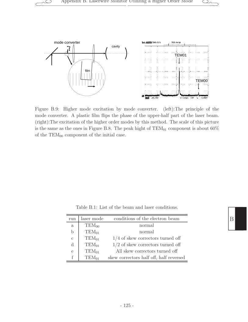
Appendix B. Laserwire Monitor Utilizing a Higher Order Mode
TEM00
TEM01
film
cavitymode converter
Figure B.9: Higher mode excitation by mode converter. (left):The principle of the
mode converter. A plastic film flips the phase of the upper-half part of the laser beam.
(right):The excitation of the higher order modes by this method. The scale of this picture
is the same as the ones in Figure B.8. The peak hight of TEM01 component is about 60%
of the TEM00 component of the initial case.
Table B.1: List of the beam and laser conditions.
run laser mode conditions of the electron beam
a TEM00 normal
b TEM01 normal
c TEM01 1/4 of skew correctors turned off
d TEM01 1/2 of skew correctors turned off
e TEM01 All skew correctors turned off
f TEM01 skew correctors half off, half reversed
- 125 -
B
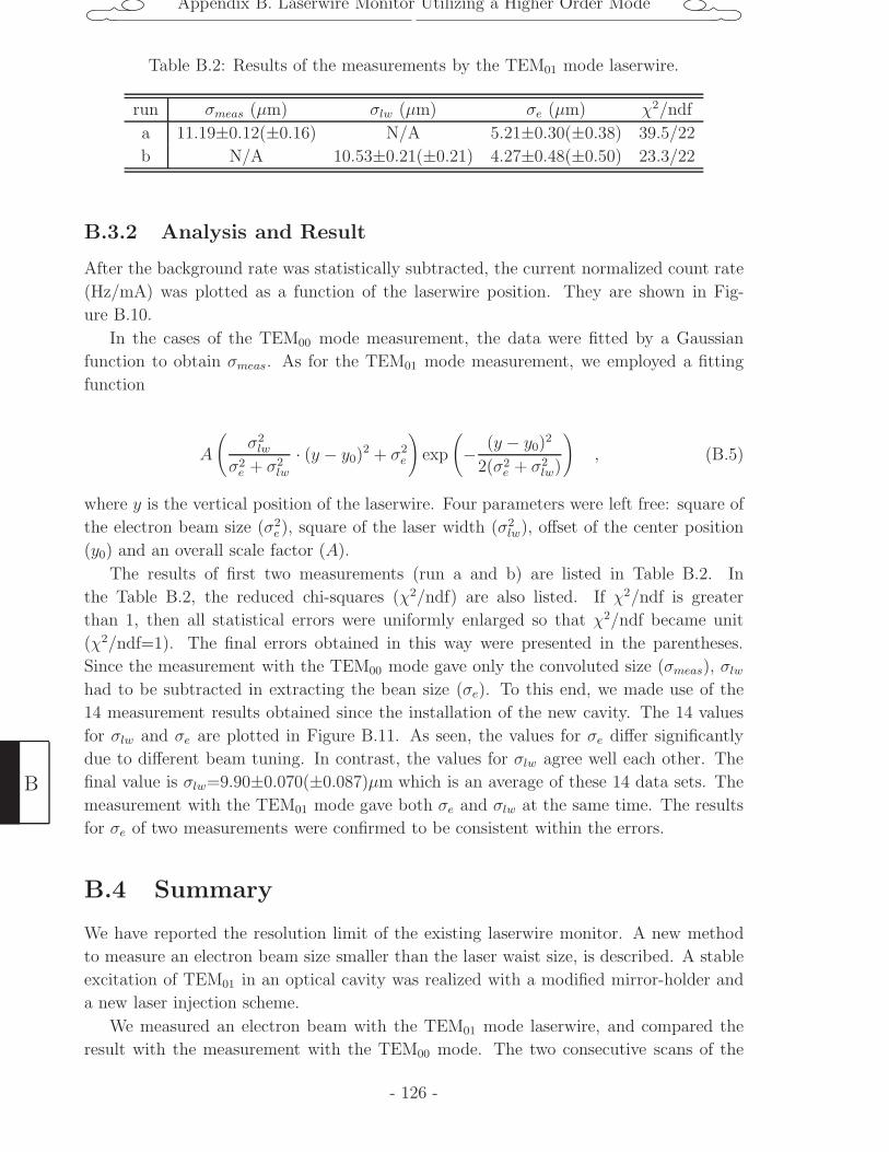
Appendix B. Laserwire Monitor Utilizing a Higher Order Mode
Table B.2: Results of the measurements by the TEM01 mode laserwire.
run σmeas (µm) σlw (µm) σe (µm) χ2/ndf
a 11.19±0.12(±0.16) N/A 5.21±0.30(±0.38) 39.5/22
b N/A 10.53±0.21(±0.21) 4.27±0.48(±0.50) 23.3/22
B.3.2 Analysis and Result
After the background rate was statistically subtracted, the current normalized count rate
(Hz/mA) was plotted as a function of the laserwire position. They are shown in Fig-
ure B.10.
In the cases of the TEM00 mode measurement, the data were fitted by a Gaussian
function to obtain σmeas. As for the TEM01 mode measurement, we employed a fitting
function
A
(σ2
lw
σ2e + σ2
lw
· (y − y0)2 + σ2
e
)exp
(− (y − y0)
2
2(σ2e + σ2
lw)
), (B.5)
where y is the vertical position of the laserwire. Four parameters were left free: square of
the electron beam size (σ2e), square of the laser width (σ2
lw), offset of the center position
(y0) and an overall scale factor (A).
The results of first two measurements (run a and b) are listed in Table B.2. In
the Table B.2, the reduced chi-squares (χ2/ndf) are also listed. If χ2/ndf is greater
than 1, then all statistical errors were uniformly enlarged so that χ2/ndf became unit
(χ2/ndf=1). The final errors obtained in this way were presented in the parentheses.
Since the measurement with the TEM00 mode gave only the convoluted size (σmeas), σlw
had to be subtracted in extracting the bean size (σe). To this end, we made use of the
14 measurement results obtained since the installation of the new cavity. The 14 values
for σlw and σe are plotted in Figure B.11. As seen, the values for σe differ significantly
due to different beam tuning. In contrast, the values for σlw agree well each other. The
final value is σlw=9.90±0.070(±0.087)µm which is an average of these 14 data sets. The
measurement with the TEM01 mode gave both σe and σlw at the same time. The results
for σe of two measurements were confirmed to be consistent within the errors.
B.4 Summary
We have reported the resolution limit of the existing laserwire monitor. A new method
to measure an electron beam size smaller than the laser waist size, is described. A stable
excitation of TEM01 in an optical cavity was realized with a modified mirror-holder and
a new laser injection scheme.
We measured an electron beam with the TEM01 mode laserwire, and compared the
result with the measurement with the TEM00 mode. The two consecutive scans of the
B
- 126 -
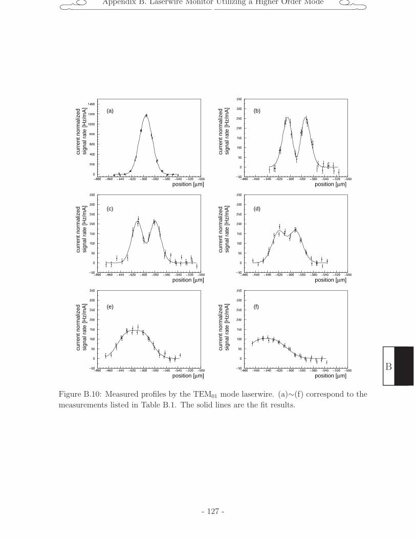
Appendix B. Laserwire Monitor Utilizing a Higher Order Mode
position [µm]
position [µm]
position [µm]
position [µm]
position [µm]
curr
ent n
orm
aliz
edsi
gnal
rat
e [H
z/m
A]
curr
ent n
orm
aliz
edsi
gnal
rat
e [H
z/m
A]
curr
ent n
orm
aliz
edsi
gnal
rat
e [H
z/m
A]
curr
ent n
orm
aliz
edsi
gnal
rat
e [H
z/m
A]
curr
ent n
orm
aliz
edsi
gnal
rat
e [H
z/m
A]
(a)
(c)
(e)
(b)
(d)
position [µm]
curr
ent n
orm
aliz
edsi
gnal
rat
e [H
z/m
A]
(f)
Figure B.10: Measured profiles by the TEM01 mode laserwire. (a)∼(f) correspond to the
measurements listed in Table B.1. The solid lines are the fit results.
- 127 -
B
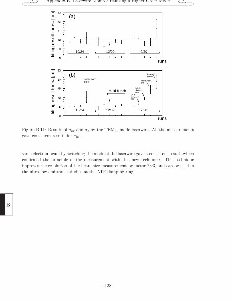
Appendix B. Laserwire Monitor Utilizing a Higher Order Mode
runs
runs
fittin
g re
sult
for
σlw [µ
m]
fittin
g re
sult
for
σe [µ
m]
10/24 12/09 2/20
10/24 12/09 2/20
multi-bunch
skew corr.OFF
1/4 of skew corr.OFF
1/2 of skew corr.OFF
All skew corr.OFF
skew corr.reverse
(a)
(b)
Figure B.11: Results of σlw and σe by the TEM01 mode laserwire. All the measurements
gave consistent results for σlw.
same electron beam by switching the mode of the laserwire gave a consistent result, which
confirmed the principle of the measurement with this new technique. This technique
improves the resolution of the beam size measurement by factor 2∼3, and can be used in
the ultra-low emittance studies at the ATF damping ring.
B
- 128 -
Appendix C. Latest Results of the Multi-Bunch Measurement
Appendix C
Latest Results of the Multi-Bunch
Measurement
The bunch intensity designed for a linear collider is 0.75×10¹⁰ e/bunch, which corresponds
to the total current of 50 mA for 20-bunches beam in ATF damping ring. The experiments
described in Sec. 5.3 and Sec. 5.4 were performed with a relatively low beam intensity.
The highest beam current measured was 20mA, only 40% of the requirement.
Since 2004, ATF started to operate a high current multi-bunch beam. In this appendix,
we report the progress in the spring runs of 2004.
C.1 Change in the laserwire setup
As explained in Appendix B, we replaced the horizontal-laserwire to a new cavity in
2003 summer. The parameters of new cavity was designed to maximize the sensitivity
of TEM01 mode scan for typical ATF beam. To this end, the laser width (σlw) becomes
twice much than it used to be. As already concluded in Appendix B, the laser width of
the new cavity was σlw=9.90±0.070(±0.087) µm.
Although the TEM01 mode has an advantage in the measurement of small beam, its
sensitive region is limited for large beam. Since there may be a strong beam blow-up in
the case of high-current multi-bunch beam, we utilized the normal TEM00 mode in this
study.
C.2 Data taking
The experiment was done on May 18, 2004. Prior to the multi-bunch measurement, we
did the usual damping ring tuning procedures in single bunch mode. Then, we switched
to multi-bunch mode and tuned the beam injection. Due to the strong beam loading effect
of high intensity multi-bunch beam, a precise tuning of energy compensation system of
linac was necessary to efficiently inject all bunches. After a careful tuning of the electron
gun and the linac, we succeeded in storing 50mA with 20-bunch beam.
When high current beam was stored in the ring, the vacuum pressure was increased
due to the huge amount of synchrotron radiation hit on the beam chamber. The growth
- 129 -
C
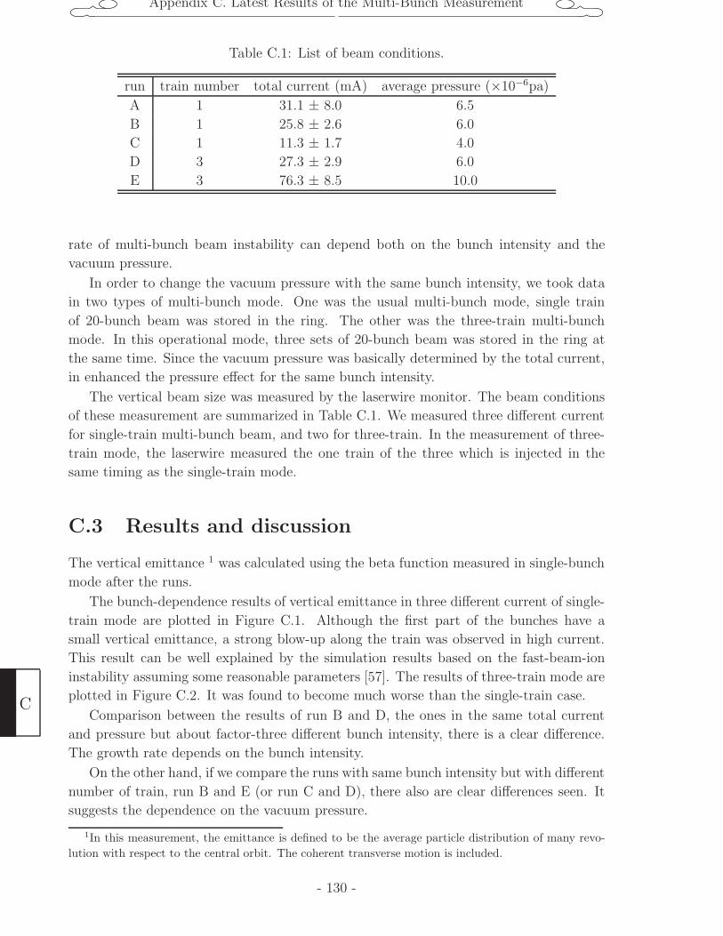
Appendix C. Latest Results of the Multi-Bunch Measurement
Table C.1: List of beam conditions.
run train number total current (mA) average pressure (×10−6pa)
A 1 31.1 ± 8.0 6.5
B 1 25.8 ± 2.6 6.0
C 1 11.3 ± 1.7 4.0
D 3 27.3 ± 2.9 6.0
E 3 76.3 ± 8.5 10.0
rate of multi-bunch beam instability can depend both on the bunch intensity and the
vacuum pressure.
In order to change the vacuum pressure with the same bunch intensity, we took data
in two types of multi-bunch mode. One was the usual multi-bunch mode, single train
of 20-bunch beam was stored in the ring. The other was the three-train multi-bunch
mode. In this operational mode, three sets of 20-bunch beam was stored in the ring at
the same time. Since the vacuum pressure was basically determined by the total current,
in enhanced the pressure effect for the same bunch intensity.
The vertical beam size was measured by the laserwire monitor. The beam conditions
of these measurement are summarized in Table C.1. We measured three different current
for single-train multi-bunch beam, and two for three-train. In the measurement of three-
train mode, the laserwire measured the one train of the three which is injected in the
same timing as the single-train mode.
C.3 Results and discussion
The vertical emittance 1 was calculated using the beta function measured in single-bunch
mode after the runs.
The bunch-dependence results of vertical emittance in three different current of single-
train mode are plotted in Figure C.1. Although the first part of the bunches have a
small vertical emittance, a strong blow-up along the train was observed in high current.
This result can be well explained by the simulation results based on the fast-beam-ion
instability assuming some reasonable parameters [57]. The results of three-train mode are
plotted in Figure C.2. It was found to become much worse than the single-train case.
Comparison between the results of run B and D, the ones in the same total current
and pressure but about factor-three different bunch intensity, there is a clear difference.
The growth rate depends on the bunch intensity.
On the other hand, if we compare the runs with same bunch intensity but with different
number of train, run B and E (or run C and D), there also are clear differences seen. It
suggests the dependence on the vacuum pressure.
1In this measurement, the emittance is defined to be the average particle distribution of many revo-lution with respect to the central orbit. The coherent transverse motion is included.
C
- 130 -
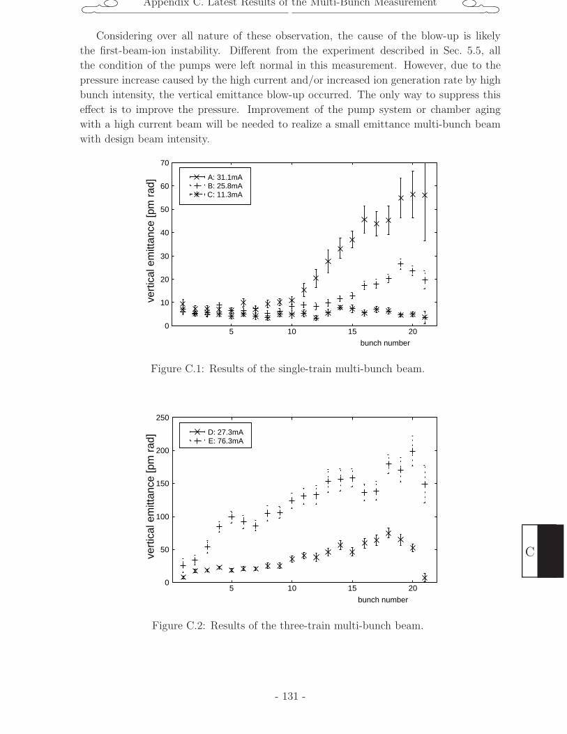
Appendix C. Latest Results of the Multi-Bunch Measurement
Considering over all nature of these observation, the cause of the blow-up is likely
the first-beam-ion instability. Different from the experiment described in Sec. 5.5, all
the condition of the pumps were left normal in this measurement. However, due to the
pressure increase caused by the high current and/or increased ion generation rate by high
bunch intensity, the vertical emittance blow-up occurred. The only way to suppress this
effect is to improve the pressure. Improvement of the pump system or chamber aging
with a high current beam will be needed to realize a small emittance multi-bunch beam
with design beam intensity.
0
10
20
30
40
50
60
70
5 10 15 20
vert
ical
em
ittan
ce [p
m r
ad]
bunch number
A: 31.1mAB: 25.8mAC: 11.3mA
Figure C.1: Results of the single-train multi-bunch beam.
0
50
100
150
200
250
5 10 15 20
vert
ical
em
ittan
ce [p
m r
ad]
bunch number
D: 27.3mAE: 76.3mA
Figure C.2: Results of the three-train multi-bunch beam.
- 131 -
C
Bibliography
[1] R. Brinkmann,et al. (eds.),
“TESLA Technical Design Report”;
DESY-2001-011, March 2001.
[2] T.O. Raubenheimer, ed. [NLC ZDR Design Group],
“Zeroth order design report for the Next Linear Collider”;
SLAC-R-0474 (1996).
[3] “GLC Project”; KEK Report 2003-7.
[4] G. Guignard, ed. [The CLIC Study Team],
“A 3 TeV e+/e- Linear Collider Based on CLIC Technology”;
Report CERN 2000-008 (July 2000).
[5] P. Raimondi and A. Seiri,
“Novel Final Focus Design for Future Linear Colliders”;
Phys. Rev. Lett. 86 (2001) 3779.
[6] International Linear Collider Technical Review Committiee,
“ILC-TRC Second Report”.
[7] R.Alley et al.,
”A laser-based beam profile monitor for the SLC/SLD interaction region”;
Nucl. Instrum. Meth. A 379(1996) 363.
[8] G.Blair,et al.,
in Proceedings of the European Particle Accelerator Conference,
Paris, 2002, pp.1912-1914.
[9] T.Shintake,
”Proposal of Nanometer beam size monitor for e+e− linear colliders”;
Nucl. Instrum. Meth. A 311(1992) 453.
[10] Edited by F. Hinode, S.Kawabata, H.Matsumoto, K.Oide, K.Takata, S.Takeda and
Urakawa,
”ATF design and study report”; KEK Internal 95-4 (1995).
[11] U.Keller,
“Recent development in compact ultrafast lasers”;
nature vol.424 (2003) 831.
- 132 -

[12] H.Hayano, private communication.
[13] C5680, Hamamatsu Photonics.
[14] H. Hayano,
“Wire scanners for small emittance beam measurement in ATF”;
The Proceedings of 20th Linear accelerator conference (2000),
http://linac2000.slac.stanford.edu/
[15] T. Naito,et al.,
in Proceedings of the Particle Accelerator Conference,
New York, 1999, pp.2143-2145.
[16] K.Iida et al.,
”Measurement of an electron-beam size with a beam profile monitor using fresnel
zone plates”;
Nucl. Instr. Method A 506(2003) p41-49.
[17] T.Muto et al..
“Observation of Incoherent Diffraction Radiation from a Single-Edge Target in the
Visible-Light Region”;
Phys. Rev. Lett. 90 (2003) 104801.
[18] Leica SMART 310, Noecross , Georgia 30071.
[19] M. Ross, J. Nelson, M. Woodley, A. Wolski,
SLAC-PUB-9239,Jun 2002. 4pp.
[20] K. Kubo ,
” Simulation stuey of low emittance tuning of the Accelerator Test Facility damping
ring at KEK”;
Phys. Rev. Special Topics - Accelerator and Beams, 6, 092801 (2003).
[21] SAD is a computer program for accelerator design.
http://acc-physics.kek.jp/SAD/sad.html
[22] H.Sakai et al.,
”Performance studies of a laser wire beam profile monitor”;
Jpn. J. Appl. Phys 41 (2002) 6398.
[23] H.Sakai, Doctor thesis submitted to Kyoto University (2002).
[24] Y.Honda et al.,
”Upgraded Laser Wire Beam Profile Monitor”;
Nucl. Instr. Meth., accepted for publication.
[25] M.E.Peskin and D.V.Schroeder,
“An Introduction to Quantum Field Theofy”; Addison-Wesley (Massachusetts, 1995).
- 133 -
[26] A.Yariv ,
”Optical Electronics”;
holts, Rinehart and Winston, (New York, 1991), 4th ed.
[27] N.Hodgson and H.Weber,
”Optical Resonators”; Springer (1997).
[28] Series 142 Diode-pumped single-frequency CW green laser, LightWave.
[29] Research Electro-Optics, Inc. (REO); Boulder, Colorado.
[30] Y.Honda,
Master thesis of Kyoto University, (2001: in japanese, unpublished).
[31] users manual of LC2440 and LB040 Series; Keyence.
[32] C7884 Linear Image Sensor; Hamamatsu Photonics.
[33] Y.Honda, K.Kubo et al.,
“Achievement of ultra-low emittance beam in the ATF damping ring”;
Phys. Rev. Lett. 92, 054802 (2004)
[34] “ATF Accelerator Test Facility Study Report JFY 1996-1999”;
KEK internal Report No. 2000-6, edited by H. Hayano et al., 2000, (unpublished).
[35] T. Okugi et al.
“Evaluation of extremely small horizontal emittance”;
Phys. Rev. Special Topics- Accelerator and Beams 2, 022801 (1999)
[36] J. Urakawa,
in Proceedings of the Seventh European Particle Accelerator Conference,
Vienna, 2000, pp.63-67.
[37] K.Kubo et al.,
“Extremely Low Vertical Emittance Beam in Accelerator Test Facility at KEK”;
Phys. Rev. Lett. 88, 19 (2002)
[38] K.L.F. Bane et al.,
” Intrabeam Scattering Analysis of measurement at KEK’s ATF damping ring”;
Phys. Rev. Special Topics - Accelerator and Beams, 5, 084403 (2002)
[39] H.Sakai et al.,
”Measurement of a small vertical emittance with a laser wire beam profile monitor”;
Phys. Rev. Special Topics - Accelerator and Beams, 5, 122801 (2002)
[40] N.Terunuma et al.
“Impedance Measurement of ATF DR”;
in Proceedings of the Sixth European Particle Accelerator Conference, Stockholm,
1998, 481.
- 134 -

[41] Y.Honda et al.,
”Measurement of electron beam emittance in the ATF damping ring operated in
multi-bunch modes“;
Phys. Rev. Special Topics - Accelerator and Beams, 6, 092802 (2003)
[42] T. Naito, private communication.
[43] J.Byrd et al.,
“First Observations of a “Fast Beam Ion Instability” ”;
Phys. Rev. Lett. 79, 79 (1997).
[44] M.Kwon et al.,
“Experimental results on the fast beam-ion instability”;
Phys. Rev. E. 57, 6016 (1998).
[45] J.Y.Huang et al.,
“Direct Observation of the Fast Beam-Ion Instability”;
Phys. Rev. Lett. 81, 4388 (1998).
[46] “CAS Fifth General Accelerator Physics Course”; CERN 94-01 (1994).
“CAS Fifth Advanced Accelerator Physics Course”; CERN 95-06 (1995).
[47] H.Wiedemann,
“Particle Accelerator Physics”; Springer Verlag, New York, 2nd ed.
[48] M.Sands,
“The Physics of Electron Storage Rings”; SLAC-121 (1970).
[49] T.Okugi,
“Evaluation of vertical emittance in KEK-ATF by utilizing lifetime measurement”;
Nucl. Instr. Meth. A 455 (2000) 207-212,
[50] A.Piwinski,
in Handbook of Accelerator Physics; World Scientific (1999) p125.
[51] J.Bjorken and S.Mtingwa;
Part. Accel 13, (1983) 115.
[52] T.O.Raubenheimer and F.Zimmermann,
“Fast beam-ion instability. I. Linear theory and simulations”;
Phys. Rev. E 52, 5487-5498 (1995).
[53] G.V.Stupakov, T.O.Raubenheimer and F.Zimmermann,
“Fast beam-ion instability. II. Effect of ion decoherence”;
Phys. Rev. E 52, 5499-5504 (1995).
[54] Y.Honda et al., in preparation.
[55] ZYGO; Laurel Brook Road Middlefield, CT
- 135 -
[56] F. Bayer-Helms,
”Coupling coefficients of an incident wave and the modes of the spherical optical
resonator in the case of mismatching and misalignment”;
Applied. Optics, Vol.23, No.9 , 1368 (1984)
[57] T.O.Raubenheimer, private communication.
- 136 -
NOTES
01
23
45
67
89
10
- 137 -

NOTES0
12
34
56
78
910
1112
1314
1516
1718
1920
2122
2324
25
- 138 -