Embed Size (px)
Citation preview

EXPERIMENTAL AND NUMERICAL STUDIES OF
THREE-PHASE RELATIVE PERMEABILITY ISOPERMS
FOR HEAVY OIL SYSTEMS
A Thesis
Submitted to the Faculty of Graduate Studies and Research
In Partial Fulfillment of the Requirements
For the Degree of
Doctor of Philosophy
In
Petroleum Systems Engineering
University of Regina
By
Manoochehr Akhlaghinia
Regina, Saskatchewan
November, 2013
Copyright 2013: M. Akhlaghinia

UNIVERSITY OF REGINA
FACULTY OF GRADUATE STUDIES AND RESEARCH
SUPERVISORY AND EXAMINING COMMITTEE
Manoochehr Akhlaghinia, candidate for the degree of Doctor of Philosophy in Petroleum Systems Engineering, has presented a thesis titled, Experimental and Numerical Studies of Three-Phase Relative Permeability Isoperms for Heavy Oil Systems, in an oral examination held on October 3, 2013. The following committee members have found the thesis acceptable in form and content, and that the candidate demonstrated satisfactory knowledge of the subject material. External Examiner: *Dr. Ian Gates, University of Calgary
Co-Supervisor: Dr. Farshid Torabi, Petroleum Systems Engineering
Co-Supervisor: Dr. Christine Chan, Petroleum Systems Engineering
Committee Member: Dr. Fotini Labropulu, Department of Mathematics and Statistics
Committee Member: Dr. Fanhua Zeng, Petroleum Systems Engineering
Committee Member: **Dr. Paitoon Tontiwachwuthikul, Industrial Systems Engineering
Committee Member: Dr. Daoyong Yang, Petroleum Systems Engineering
Chair of Defense: Dr. Sandra Zilles, Department of Mathematics & Statistics *Participated via Tele-conference **Not present at defense
i
ABSTRACT
There is a great deal of interest in obtaining reliable three-phase relative
permeability data given recent developments in enhanced heavy oil recovery processes
associated with multiphase flow in porous media. Experimental measurement of three-
phase relative permeability data for heavy oil systems is prohibitively difficult. Such data
and research is scarce in the literature since the implementation of steady state
experiment is onerous and time consuming. Still results from unsteady state technique do
not really coincide with those from steady state experiments. Empirical correlations, such
as Stone’s models, which are widely used in modern commercial simulators, carry along
uncertainties with two-phase relative permeabilities. In addition, their applicability to
heavy oil systems has not been proven.
This work proposes a procedure to utilize two- and three-phase unsteady state
displacements in order to estimate three-phase relative permeability isoperms. Using
residual oil and irreducible water saturations obtained from two-phase heavy oil/water
floods, a three-phase flow zone in a ternary diagram was found. Three-phase
displacement was conducted in the form of gas injection into a consolidated Berea core
saturated with heavy oil and water. A lab-scale three-phase one-dimensional simulator
was developed and validated to simulate three-phase displacement experiments.
Appropriate three-phase relative permeability data was then selected according to a
saturation path drawn across the three-phase flow zone in the ternary diagram. This
relative permeability data was continuously fine-tuned until differential pressure, heavy
oil production, and water production from the numerical simulator match those from the
three-phase displacement experiment. Repeating this procedure for different saturation

ii
paths provides a set of relative permeability data which were used to plot relative
permeability isoperms for each phase in ternary diagrams.
The procedure was validated using steady state experiment and, then, used to
study the effect of temperature, oil viscosity, and different gas phase on the relative
permeability isoperms for heavy oil systems. Results from this study showed that limited
three-phase flow zones exist for heavy oil fluid systems due to high values of residual oil
saturation. Different curvatures were observed with relative permeability isoperms of all
phases. It was observed that, due to significant contrast between viscosities, oil relative
permeability values are higher than those for water and carbon dioxide in order of
magnitude of three and five, respectively.
It was found that relative permeabilities is no longer a function of saturations as
they tend to vary with change in the temperature, oil viscosity, and gas phase. The effect
of such parameters on relative permeabilities was shown to be different for each phase. In
some cases, opposite and even reversal trends were observed. For instance, oil relative
permeability in the presence of carbon dioxide was higher compared to methane, while
relative permeability to water phase was higher in presence of methane.
The proposed method takes advantage of the practicability of the unsteady state
method to provide three-phase relative permeability isoperms in a fast and reliable way. It
minimizes the uncertainties that exist with the unsteady state method, such as inaccurate
end-face saturation calculation and erroneous derivatives. Also, extensive study of
relative permeabilities in different conditions helps us to improve our understating of
three-phase relative permeabilities in simulation of processes such as thermal techniques,
Steam Assisted Gravity Drainage (SAGD), Cyclic Steam Stimulation (CSS) etc.

iii
ACKNOWLEDGEMENTS
Foremost, I would like to express my sincere gratitude to my supervisors Dr. Farshid
Torabi and Dr. Christine W. Chan for the continuous support of my PhD study and
research, for their patience, motivation, enthusiasm, and immense knowledge. Their
guidance helped me throughout my research and the writing of this thesis. I could not
have imagined having better advisors for my PhD study.
In addition to my supervisors, I would like to thank Dr. Ian D. Gates, Dr. Paitoon (P.T.)
Tontiwachwuthikul, Dr. Fotini Labropulu, Dr. Daoyong (Tony) Yang, and Dr. Fanhua
(Bill) Zeng, for their encouragement, insightful comments, and useful questions.
I would like to thank the Petroleum Technology Research Centre (PTRC), Faculty of
Graduate Studies and Research (FGSR), and Natural Sciences and Engineering Research
Council of Canada (NSERC) for funding support.
I further thank Dr. Fanhua (Bill) Zeng, and my friends Alireza Qazvini Firouz and Ryan
R. Wilton who helped me whenever I needed their support.

iv
DEDICATION
To Lovely Razieh & My Family

v
TABLE OF CONTENTS
ABSTRACT………………………………………………………………………….……i
ACKNOWLEDGEMENTS…………………………………………………………….iii
DEDICATION………………………………………………………………………..…iv
TABLE OF CONTENTS……………………………………………………….……….v
LIST OF TABLES………………………………………………………………………ix
LIST OF FIGURES………………………………………………………………….…..x
LIST OF APPENDICES…………………………………………………………….…xv
NOMENCLATURE………………………………………………………...……….…xvi
CHAPTER 1: INTRODUCTION…………………………………………………….....1
1.1 Heavy Oil Reservoirs……………………………………………………………..1
1.2 Enhanced Heavy Oil Recovery……………………………………………...……2
1.2.1 Thermal techniques………………………………………….……………..3
1.2.2 Non-thermal techniques…………………………..………………..………4
1.3 Three-Phase Relative Permeability……………………………………...………..5
1.4 Motivation and Objectives……………………………………………..…………6
1.5 Outline of the Thesis………..…………………………………………………….7
CHAPTER 2: LITERATURE REVIEW……………………………………………….9
2.1 Background……………………………………………………………………….9
2.2 Three-Phase Relative Permeability Measurements………………………….…..12
2.2.1 Steady state experiments ………………………..………………………..12
2.2.1.1 Leverett and Lewis (1941)……………………………...………….13
2.2.1.2 Caudle et al. (1951)………………………………………….……..16
2.2.1.3 Corey et al. (1956)…………………………………………..……..19
2.2.1.4 Reid (1956)…………………………………………………...……23
2.2.1.5 Snell (1962, 1963)………………………………………………….23
vi
2.2.1.6 Saraf and Fatt (1967)………………………………………………26
2.2.1.7 Oak (1988, 1990, 1991)……………………………………………26
2.2.1.8 Poulsen et al. (2000)……………………………………………….29
2.2.2 Unsteady state experiments………………………..……………..……….29
2.2.2.1 Sarem (1966)……………………………………………………….30
2.2.2.2 Donaldson and Dean (1966)……………………….………………31
2.2.2.3 Schneider and Owens (1970)………………………...…………….33
2.2.2.4 Van Spronsen (1982)……………………………………….………33
2.2.2.5 Grader and O’Meara (1988)………………………………………..35
2.2.2.6 Siddiqui et al. (1995)………………………………..……………..35
2.2.3 Three-phase relative permeability models……………..…..……………. 35
2.2.3.1 Stone I and II (1970)………………………………………………36
2.2.3.2 Hirasaki (1976)………………………………………………...…37
2.2.3.3 Aziz and Settari (1979)……………………………………...…….38
2.2.3.4 Aleman and Slattery (1988)…………………………...…………..38
2.2.3.5 Baker (1988)………………………………………………...…….39
2.2.3.6 Pope and Delshad (1989)………………………………..…………39
2.2.3.7 Kokal and Maini (1989)……………………………………..……..40
2.2.3.8 Husted and Hansen (1995)................................................................40
2.3 Parameter Estimation………………………………………………………..…..40
2.4 Chapter Summary and Statement of Problem……………………...……………42
CHAPTER 3: EXPERIMETAL SETUPS AND MATERIAL……...…..……………45
3.1 Introduction……………………………………………………………….……..45
3.2 Experimental setups………………………………………………….………….45
3.2.1 Core holder……………………………………………….……...………..49
3.2.2 Fluid injection system…………………………………....……………….49
3.2.3 Pressure transducer system…………………………….....………………50

vii
3.2.4 Fluid collection system……………………………………...……………50
3.2.5 Temperature controlling system……………………………....…………..50
3.2.6 Gas injection system……………………………………………………...51
3.2.7 Separation system……………………………………………………...…51
3.3 Core Properties…………………………………………………………………..51
3.4 Fluid Properties………………………………………………………………….54
3.4.1 Heavy oil / water properties…………………………………..…………..54
3.4.2 Gas properties………………………………………………………...…..56
3.5 Experimental Procedures………………………………………….…………….56
3.5.1 Core cleaning…………………………………………...…….…………..56
3.5.2 Two-phase heavy oil / water displacement experiment…………………..58
3.5.3 Two-phase heavy oil / gas displacement experiment……………….…….59
3.5.4 Three-phase displacement experiment………………………………..…..59
3.6 Chapter Summary…………………………………………………………….…61
CHAPTER 4: TWO-PHASE RELATIVE PERMEABILITY WITH JBN
TECHNIQUE …….……………………………………………………...……………..65
4.1 Introduction………………………………………………………………...……65
4.2 JBN Technique…………………………………………………………..………65
4.3 Two-Phase Relative Permeabilities Based on JBN Technique………………….69
4.3.1 Heavy oil / water systems……………………………………………...…69
4.3.2 Heavy oil / gas systems…………………………………………...……....74
4.4 Chapter Summary……………………………………………………………….80
CHAPTER 5: THREE-PHASE RELATIVE PERMEABILITY ISOPERMS……. 83
5.1 Introduction…………………………….…………………………………….….83
5.2 Procedure………………………………………………………………………..84
5.3 Determination of Three-Phase Flow Zone………….……………………..…… 85
5.4 Three-Phase Displacement Experiments………………………………..………92
5.5 Numerical Simulation………………………………………………………...…95
viii
5.6 Three-Phase Relative Permeability Isoperms (Base Case)…………...………..99
5.6.1 Validation of the results steady state experiments…………………...….107
5.6.2 Sensitivity analysis…………………………………………………..….113
5.7 Chapter Summary……………………………………………….……………..117
CHAPTER 6: EFFECT OF TEMPERATURE, OIL VISCOSITY, AND GAS
PHASE ON RELATIVE PERMEABILITY ISOPERMS ………………………….118
6.1 Introduction………………………………………………………………...…..118
6.2 Effect of Temperature on Three-phase Relative Permeabilities………………..118
6.3 Effect of Oil Viscosity on Heavy oil / Water / CO2 Systems……………….…122
6.4 Effect of Different Gas Phase on Heavy oil / Water / Gas Systems………...….125
6.5 Chapter Summary………………………………………………………...……127
CHAPTER 7: CONCLUSIONS AND RECOMMENDATIONS…………..………129
7.1 Conclusions……………………………………………………………...……..129
7.2 Recommendations………………………………………………………...……132
REFERNCES……………………………………………………………………...……134
APPENDIX A…………………………………………………………………………..150
APPENDIX B..................................................................................................................157
APPENDIX C…………………………………………………………..………………164
APPENDIX D…………………………………………………………………………. 177
APPENDIX E ………………………………………………………...………………..192
APPENDIX F………………………………………………………………...…………202

ix
LIST OF TABLES
Table 3.1: Basic properties of Berea core sample………………………….……………52
Table 3.2: Summary of three- phase experiments…………………………………...…..63
Table 3.3: Summary of two- phase displacement experiments…………………………64
Table 4.1: Relative permeability data calculated by JBN technique at 28ºC for heavy oil
(sample#1)/ water..………………………………………………………………….……68
Table 4.2: Summary of effect of increase in temperature on the relative permeability of
two-phase systems………………………………………………………………….……81
Table 4.3: Summary of effect of increase in oil viscosity on the relative permeability of
two-phase systems………………………………………………………………...……..82
Table 5.1: Summary of condition for four two-phase tests conducted……………...…..91
Table 5.2: Oil and water saturations before gas injections……………………….……..93
Table 5.3: Details of the model used to validate developed simulator with CMG-
IMEX………..…………………………………………………………………….……..96
Table 5.4: Relative permeability from steady state experiments………………………109
Table 6.1: Effect of different parameters on three-phase relative permeabilities……...128
x
LIST OF FIGURES
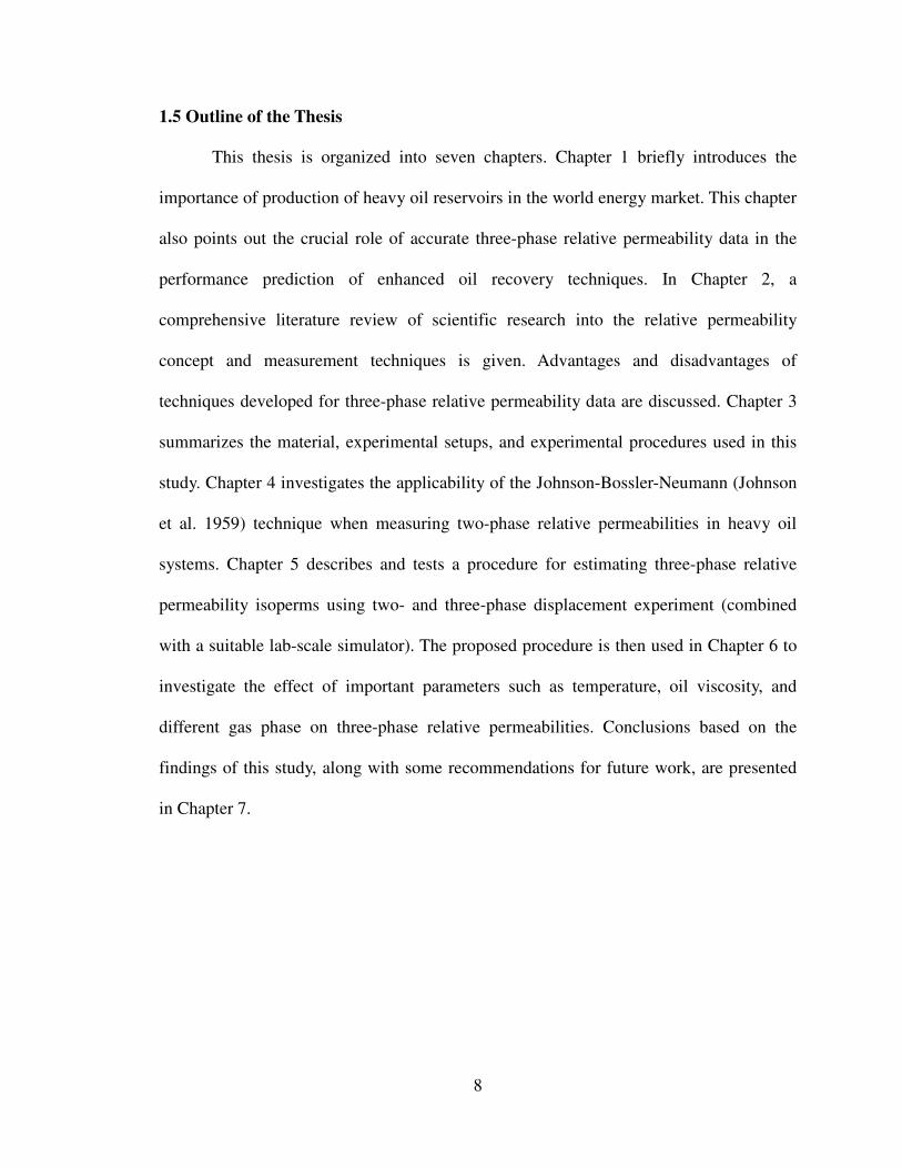
Figure 2.1: Relative permeability to water as a function of water saturation (Leverett and
Lewis, 1941)…………………………………………………………………..…………14
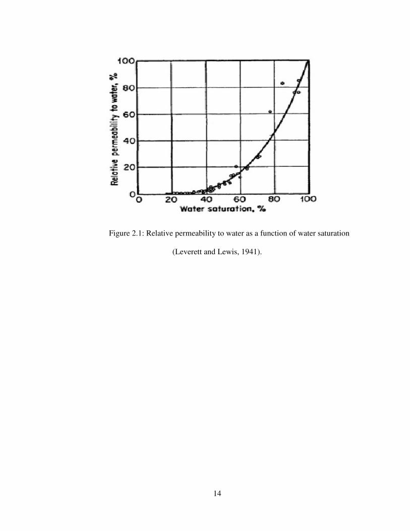
Figure 2.2: Ternary diagram of oil (a) and gas (b) relative permeability isoperms
(Leverett and Lewis, 1941)……………………………………………………..………..15
Figure 2.3: Two-phase and three-phase flow regions (Leverett and Lewis, 1941)…...…17
Figure 2.4: Three-phase relative permeability isoperms (Caudle et al., 1951)………….18
Figure 2.5: Three-phase relative permeability data (Corey et al., 1956)…………….….20
Figure 2.6: Gas and oil relative permeability versus total liquid saturation (Corey et al.,
1956)………………………………………………………………………………….….21
Figure 2.7: Three-phase relative permeability data (Reid, 1956)………………….……24
Figure 2.8: Three-phase relative permeability data (Snell, 1962)……………...……….25
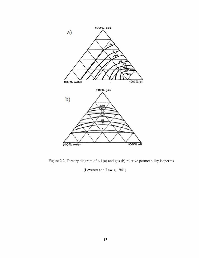
Figure 2.9: Three-phase relative permeability data (Saraf and Fatt, 1967)……….…….27
Figure 2.10: Evaluation of Stone’s model using experimental data (Oak, 1990)……….28
Figure 2.11: Unsteady state three-phase isoperms for sandstone and limestone
(Donaldson and Dean, 1966)………………………………………………….…………32
Figure 2.12: Three-phase isoperms for oil (top) and water (bottom) from centrifuge
experiment (Van Spronsen, 1982)………………………………..……….……………..34
Figure 3.1: Schematic diagram of experimental setup for heavy oil / water displacement
experiments……………………………………………………………………..……….46
Figure 3.2: Schematic diagram of the setup for two-phase (heavy oil / gas) and three-
phase displacement experiments…………………………………………………………47
Figure 3.3: Schematic diagram of the setup for three-phase steady state experiments…48
xi
Figure 3.4: Linear relationship between flow rate and differential pressure in absolute
permeability measurement……………………………………………………………....53
Figure 3.5: Viscosity versus temperature for a) heavy oil samples used in the
experiments and b) for 1wt% NaCl water..………………………………………………55
Figure 3.6: Viscosity and compressibility factor versus pressure at different temperature
for a) carbon dioxide and b) methane (from CMG-WINPROP).……………....………..57
Figure 4.1: Heavy oil / water relative permeabilities; a: (T=28°C, Oil#1), b: (T=40°C,
Oil#1), c: (T=52°C, Oil#1), d: (T=28°C, Oil#2)…………………………………………70
Figure 4.2: Effect of temperature on water (a) and heavy oil (b) relative
permeabilities………………………………………………………………………….…2
Figure 4.3: Effect of oil viscosity on water (a) and heavy oil (b) relative
permeabilities…………………………………………………………………………….73
Figure 4.4: Heavy oil / CO2 relative permeabilities; a: (T=28°C, Oil#1), b: (T=40°C,
Oil#1), c: (T=52°C, Oil#1), d: (T=28°C, Oil#2)……………………………...………….75
Figure 4.5: Heavy oil / CH4 relative permeabilities; a: (T=28°C, Oil#1), b: (T=40°C,
Oil#1), c: (T=52°C, Oil#1), d: (T=28°C, Oil#2)………………………….……………..76
Figure 4.6: Effect of temperature on heavy oil / gas relative permeabilities; a and b
(CH4), c and d (CO2)……………………………………………………..………………78
Figure 4.7: Effect of oil viscosity on heavy oil / gas relative permeabilities; a and b
(CH4), c and d (CO2)……………................………………………….………………….79

xii
Figure 5.1: Saturation path selection through the three-phase zone (original in
color)..................................................................................................……………………86
Figure 5.2: Procedure used to estimate three-phase relative permeability data from
unsteady state displacement experiments……………………………………….……….87
Figure 5.3: Typical three-phase flow zone for heavy oil/water/gas system (original in
color).........................................................................................................…....………….88
Figure 5.4: Average water saturation change during oil injection…………….………..89
Figure 5.5: Average oil saturation change during water injection………………………90
Figure 5.6: Results from three-phase displacement for base case (carbon dioxide
injection at 28°C)………………………………………………………….…………..…94
Figure 5.7: Relative permeability data used to validate developed simulator with CMG-
IMEX; a: oil/water relative permeability, b: liquid/gas relative permeability…….……97
Figure 5.8: Comparing results from generated simulator with CMG-IMEX using a
generic model……………...……………………………………………………...….….98
Figure 5.9: Results from matching test#1 for saturation path # 1, top (pressure drop),
middle (oil production), and bottom (water production)…………………....………..….98
Figure 5.10: Results from matching test#1 for saturation path # 2, top (pressure drop),
middle (oil production), and bottom (water production)…………………………..…101
Figure 5.11: Results from matching test#1 for saturation path # 3, top (pressure drop),
middle (oil production), and bottom (water production)……………………...………..102
xiii
Figure 5.12: Oil relative permeability isoperms from test#1(original in color)
………….....….………...................................................................................................104
Figure 5.13: Water relative permeability isoperms from test#1 (×E+03) (original in
color).........................................................................................................……….……..105
Figure 5.14: Carbon dioxide relative permeability isoperms from test#1 (×E+05)
(original in color).....................................................................................................…....106
Figure 5.15: Validation of oil relative permeability isoperms with steady state tests
(original in color).........................................................................................................…110
Figure 5.16: Validation of water relative permeability isoperms with steady state tests
(original in color).......................................……………………………………………..111
Figure 5.17: Validation of gas relative permeability isoperms with steady state tests
(original in color)...........................……………………………………………………..112
Figure 5.18: Effect of change in oil relative permeability data on the pressure drop
predicted by the numerical simulator………………………………………..………….114
Figure 5.19: Effect of change in water relative permeability data on the pressure drop
predicted by the numerical simulator……………………………………..…………….115
Figure 5.20: Effect of change in CO2 relative permeability data on the pressure drop
predicted by the numerical simulator…………………………………………….……..116
xiv
Figure 6.1: Relative permeability isoperms for heavy oil / water / CO2 system of fluids
from left to right: 28°C, 40°C, 52°C. Red (kro), Blue (krw×E+03), Yellow (krg×E+05)
(original in color)......................................…………………………..………………….120
Figure 6.2: Relative permeability isoperms for heavy oil / water / CH4 system of fluids
from left to right: 28°C, 40°C, 52°C. Red (kro), Blue (krw×E+03), Yellow (krg×E+05)
(original in color)…..........……………………….................................………………..121
Figure 6.3: Relative permeability isoperms for heavy oil / water / CO2 system of fluids.
Left (Oil Viscosity = 1174 cP), Right (Oil Viscosity = 2658 cP). Red (kro), Blue
(krw×E+03), Yellow (krg×E+05) (original in color)....…...........…….……..………….123
Figure 6.4: Relative permeability isoperms for heavy oil / water / CH4 system of fluids.
Left (Oil Viscosity = 1174 cP), Right (Oil Viscosity = 2658 cP). Red (kro), Blue
(krw×E+03), Yellow (krg×E+05) (original in color).....................................…………..124
Figure 6.5: Relative permeability isoperms for heavy oil / water / gas system of fluids.
Left (CO2), Right (CH4). Red (kro), Blue (krw×E+03), Yellow (krg×E+05) (original in
color)...............................................................................................................……...…. 124

xv
LIST OF APPENDICES
APPENDIX A: EXPERIMENTAL SETUP…………………………………...………151
APPENDIX B: RESULTS OF THREE-PHASE DISPLACEMENT TESTS……...…158
APPENDIX C: MATHEMATICAL MODEL OF DEVELOPED SIMULATOR…....165
APPENDIX D: MATLAB CODE FOR DEVELOPED SIMULATOR………….….. 178
APPENDIX E: 3RELPERM PLOT……………………………………….…………..193
APPENDIX F: FINAL MATCHING RESULTS……………………………………..202

xvi
NOMENCLATURE
A area ft2
Bg gas formation volume factor bbl/scf
Bo oil formation volume factor bbl/STB
Bw water formation volume factor bbl/STB
k absolute permeability Darcy
kr relative permeability Fraction
krgo two-phase relative permeability to gas in oil/gas system Fraction
kro three-phase relative permeability to oil Fraction
krog two-phase relative permeability to oil in oil/gas system Fraction
krow two-phase relative permeability to oil in oil/water system Fraction
krwo two-phase relative permeability to water in oil/water system Fraction
P pressure Psia
qgsc gas flow rate scf/D
qosc oil flow rate STB/D
qwsc water flow rate STB/D
S saturation fraction
Sg gas saturation fraction
Som three-phase residual oil saturation fraction
Sor residual oil saturation fraction
Sorg two-phase residual oil saturation in oil/gas system fraction
Sorw two-phase residual oil saturation in oil/water system fraction

xvii
Sw water saturation fraction
Swc connate water saturation fraction
Swi irreducible water saturation fraction
T absolute temperature ºR
t time day
x length ft
Z compressibility factor dimensionless
αc volume conversion factor dimensionless
βc transmissibility conversion factor dimensionless
βg defined by Equation (2.15)
βw defined by Equation (2.15)
µ viscosity cP
φ porosity fraction
Subscripts
g gas
max maximum
nor normalized saturation
o oil
og oil/gas system
s normalized relative permeability according to Equations (2.29) to (2.32)
w water
wg water/gas system

xviii
wo water/oil system
σ probability function defined by Equations (2.21) and (2.22)
Abbreviations
PV pore volume
FVF formation volume factor

1
CHAPTER 1
INTRODUCTION
1.1 Heavy Oil Reservoirs
By definition, heavy oils are considered to have an API (American Petroleum
Institute) gravity that is less than 20 (Meyer and Dietzman, 1979). Although this
definition is widely used in the petroleum industry (Parker et al., 1986), many researchers
and engineers may use viscosity to describe the flow characteristics of crude oil (Gibson,
1982). This might be because some low API gravity crude oils have been reported to
show considerably low viscosities at reservoir temperatures when compared to high API
gravity crude oils (Briggs et al., 1988). Although there are several categories of heavy
oils, all crude oils with viscosities of more than 100 cP must be stimulated in order to be
recovered, and therefore, are considered heavy oils (Briggs et al., 1988).
According to the International Energy Agency reports, heavy oil reservoirs, which
represent almost 50 percent of the world's recoverable oil resources, will play a vital role
in quenching the growing demand of world economies for energy (Marin et al., 2008;
IEA, 2010). Among those countries with heavy oil resources, Canada (Alberta and
Saskatchewan) and Venezuela (Orinoco Belt) are at the forefront of heavy oil production,
with 45% and 25%, respectively, of all oil productions coming from heavy oil resources
(Dusseault, 2001; Ghannam et al., 2012).

2
1.2 Enhanced Heavy Oil Recovery
Enhanced oil recovery refers to the stages of oil recovery that are beyond primary
production and waterflooding. In the case of heavy oil and bitumen, with minor or no
primary production and/or waterflooding, enhanced oil recovery is the first step. A
summary of known enhanced oil recovery techniques developed for light and heavy oils
are given below (Farouq Ali and Thomas, 1994):
• Non-Thermal Techniques
o Chemical Flooding
� Polymer Flooding
� Surfactant Flooding
� Alkaline Flooding
o Miscible Displacements
� Enriched Gas Drive
� Vaporizing Gas Drive
� Alcohol Flooding
� Carbon Dioxide Flooding
� Nitrogen Flooding
o Gas Drives
� Inert Gas
� Flue Gas
� Immiscible Carbon Dioxide
� (Vapor Extraction) VAPEX
• Thermal Techniques
o Steam Injection
� Cyclic Steam Stimulation (CSS)
� Steam Flooding
� Huff and Puff
� Steam Assisted Gravity Drainage (SAGD)

3
o Hot Water Flooding
o In-Situ Combustion
o Electrothermal Heating
• Other Techniques
o Mining
o Cold Heavy Oil Production from Sands (CHOPS)
o Microbial Techniques
The level of interest in different enhanced oil recovery techniques strongly
depends on the oil price which, in turn, depends on the world economy and political
situation. In fact, the number of field projects for enhanced oil recovery techniques is not
necessarily related to its success or effectiveness (Farouq Ali and Thomas, 1994).
1.2.1 Thermal techniques
Thermal techniques are more widely applied in sandstone formations when
compared to gas injection methods (Alvarado and Manrique, 2010). Cyclic steam
injection (or Huff & Puff), steam flooding, and most recently, Steam Assisted Gravity
Drainage (SAGD) have been the most widely used recovery methods for heavy and extra-
heavy oil in sandstone reservoirs during the last decades. For instance, Canada, Former
Soviet Union, United States, Venezuela, Brazil, and China to a lesser extent, have utilized
these techniques (De Haan and Van Lookeren, 1969; Hanzlik, 2003; Ramlal, 2004;
Jelgersma, 2007; Lacerda et al., 2008; Ernandez, 2009).
Steam injection and SAGD represent two important thermal enhanced oil
recovery techniques to increase oil production in the oil sands. SAGD has received
attention in Canada and Venezuela, owing vast heavy and extra-heavy oil reserves due to

4
applicability in unconsolidated reservoirs with high vertical permeability (Manrique and
Pereira, 2007).
In-situ combustion is considered the second most important recovery method for
heavy crude oils. Despite the large number of inconclusive or failed pilots, perhaps due to
lack of understanding of the process and applications in reservoirs, there are several
ongoing in-situ combustion projects in heavy oil reservoirs in Canada (Moritis, 2008),
Romania (Machedon et al., 1994; Panait-Paticaf et al., 2006), India (Roychaudhury et al.,
1997; Sharma et al., 2003; Chattopadhyay et al., 2004; Doraiah et al., 2007) and the
United States (Long and Nuar, 1982).
Other approaches to thermal enhanced oil recovery methods, such as Toe-to-Heel
Air Injection (THAI) (Xia et al., 2002; Greaves et al., 2005) and Electrothermal heating
(Islam et al., 1991; Sierra et al., 2001; Hascakir et al., 2008; Rodriguez et al., 2008; Das,
2008), have been proposed, yet have had little or no impact on heavy oil production.
1.2.2 Non-thermal techniques
Chemical methods, the most important non-thermal enhanced oil recovery
techniques, were widely applied in the 1980s. However, since the 1990’s, oil production
from chemical methods have been negligible around the world, except for China and the
Netherlands to a lesser extent (Moritis, 2008).
Polymer flooding, the most important chemical enhanced oil recovery, is mostly
used in China, with almost 20 ongoing projects. In addition to polymers, the injection of
alkali, surfactant, alkali-polymer (AP), surfactant-polymer (SP), and Alkali-Surfactant-
Polymer (ASP) have been conducted in a limited number of pilot projects (Moritis,

5
2008). Although chemical recovery methods were seen as promising approaches since
1980, the high concentrations and cost of chemicals, combined with low oil prices during
1990s, limited their use. However, the development of technology and surfactant
chemistry have led to a renewed interest in chemical floods in recent years, especially in
enhanced oil production in mature and waterflooded fields (Bou-Mikael, 2000).
Gas flooding is considered a non-thermal technique suitable for recovery from
light, condensate, and volatile oil reservoirs. Although ongoing field implementation of
nitrogen injection is very limited, it is believed to increase oil recovery under miscible
conditions favouring the vaporization of light fractions of light oils and condensates
(Moritis, 2008). Except North Alaska, where large natural gas resources are available
without transportation expenses, hydrocarbon gas injection projects in onshore sandstone
reservoirs have not made a significant impact on oil recovery in Canada and the United
States. Pressure maintenance projects with gas and Water Alternate Gas (WAG)
processes have been shown to be more promising as compared to gas injections (Moritis,
2008).
1.3 Three-Phase Relative Permeability
The dependency of international economies on energy from heavy oil resources
has led the petroleum industry to develop several enhanced oil recoveries techniques.
Numerical reservoir simulators have become a major tool in production optimization and
performance prediction of all enhanced oil recovery processes (Ambastha and Kumar,
1999; Esmail, 1985). Relative permeability data is essential for any kind of reservoir
development that describes the mechanism of a multiphase flow through reservoir. There
are several studies in the literature that have addressed the significant role of three-phase

6
relative permeability data in numerical simulations of different enhanced oil recovery
techniques, such as Water Alternate Gas injection (WAG) (Land, 1968; Christensen et al.,
2001; Element et al, 2003; Spiteri and Juanes, 2006; Shahverdi et al., 2011), Cyclic
Steam Stimulation (CSS) (Dietrich, 1981; Lake, 1989; Dria et al., 1993), gas injections
(Muqeem et al., 1993; kalaydjian et al., 1996; Shojaei et al., 2012), in-situ combustion
(Schneider and Owens, 1970), Surfactant flooding (Foulser et al., 1992), Steam Assisted
Gravity Drainage (SAGD) process (Chalier et al., 1995), Gas Assisted Gravity Drainage
(GAGD) process (Blunt et al., 1995), and CO2 geological sequestrations in depleted
reservoirs (Koide et al., 1992).
In the past decades, numerous attempts have been made to reduce uncertainty in
the input data of the numerical simulators (Capen, 1976; Hastings et al., 2001; Caldwell
and Heather, 2001). Inaccurate relative permeability data is said to be a major source of
uncertainty in performance predictions involving numerical simulators (Demond et al.,
1996; Boukadi et al., 2005). Due to the scarcity of three-phase relative permeability data,
it is often tuned or obtained by history matching. However, the manipulation of three-
phase relative permeability data can cause flow parameters to be compromised (Li and
Horne, 2008).
1.4 Motivation and Objectives
Three-phase relative permeability data obtained from steady state experiments is
rare (especially for heavy oil systems) due to the laborious nature of the procedure. As
stated in the next chapter, despite several decades of study, there is no general unsteady
state technique that provides three-phase relative permeability data consistent with that
from a steady state technique. With several proven uncertainties, modern commercial

7
reservoir simulators widely use three-phase relative permeabilities from the empirical
correlations based on two-phase relative permeability data.
This work focuses on the estimation of three-phase relative permeability data for
heavy oil systems, knowing that few available data, measurement techniques, and
correlations are based on synthetic or conventional light oils. The main objectives of this
study are as following:
• Performing two and three-phase displacement experiments with water, gas
(carbon dioxide and methane), and heavy oil.
• Investigating the feasibility of applying the Johnson-Bossler-Naumann (JBN)
technique in heavy oil systems.
• Developing and validating a three-phase, fully implicit, and one-dimensional
numerical simulator to simulate three-phase displacement experiments, since
available reservoir simulators can be supplied only with empirical correlations.
• Proposing a procedure to utilize two- and three-phase unsteady state displacement
experiments combined with developed numerical simulator in order to estimate all
relative permeability isoperms.
• Verifying estimated relative permeability isoperms with steady state experiments
and, also, through conducting sensitivity analysis.
• Investigating the effect of key parameters, such as heavy oil viscosity,
temperature, and different gas phase (carbon dioxide and methane) on three-phase
relative permeability data.
8
1.5 Outline of the Thesis
This thesis is organized into seven chapters. Chapter 1 briefly introduces the
importance of production of heavy oil reservoirs in the world energy market. This chapter
also points out the crucial role of accurate three-phase relative permeability data in the
performance prediction of enhanced oil recovery techniques. In Chapter 2, a
comprehensive literature review of scientific research into the relative permeability
concept and measurement techniques is given. Advantages and disadvantages of
techniques developed for three-phase relative permeability data are discussed. Chapter 3
summarizes the material, experimental setups, and experimental procedures used in this
study. Chapter 4 investigates the applicability of the Johnson-Bossler-Neumann (Johnson
et al. 1959) technique when measuring two-phase relative permeabilities in heavy oil
systems. Chapter 5 describes and tests a procedure for estimating three-phase relative
permeability isoperms using two- and three-phase displacement experiment (combined
with a suitable lab-scale simulator). The proposed procedure is then used in Chapter 6 to
investigate the effect of important parameters such as temperature, oil viscosity, and
different gas phase on three-phase relative permeabilities. Conclusions based on the
findings of this study, along with some recommendations for future work, are presented
in Chapter 7.

9
CHAPTER 2
LITERATURE REVIEW
2.1 Background
A porous medium is commonly represented as a solid, such as a rock, sand pack,
membrane or filter, containing void spaces or pores, either connected or disconnected,
and distributed within that solid regularly or randomly. These pores may contain a variety
of fluids, such as air, gas, water, brine, oil, etc. In addition, these pores, which represent a
portion of the bulk volume, form a complex network capable of carrying fluids through
them. Petroleum engineering, chemical engineering, hydrology, and soil mechanics,
among others, are some of the numerous disciplines in which porous media play an
important role or where the technology requires them as a tool (Heinemann, 2005).
According to the American Petroleum Institute (API) Code 27, absolute
permeability is defined with the help of Darcy’s law, Equation (2.1), as a property of
porous media and is “a measure of the capacity of the medium to transmit fluids” (Amyx
et al., 1988).
�� = − �� (��� �
�.�������� × 10��) (2.1)
where
s = distance in the direction of flow, cm
�� = volume flux across a unit area of the porous medium in unit time along flow path s,
cm/sec

10
z = vertical coordinate, cm
ρ = density of the fluid, gm/cm3
g = acceleration of gravity, 980.665 cm/sec2
dP/ds = pressure gradient along s at the point to which �� refers, atm/cm
µ = viscosity of the fluid, cP
k = absolute permeability of the medium, darcies
This term is applicable if a single fluid flows through the porous media. Because,
in petroleum reservoirs, multiphase flow is encountered, the basic definition of
permeability stated by API Code 27 needs to be modified. Accordingly, effective
permeability is used to describe simultaneous flow of more than one fluid (e.g., oil, water,
gas). In the definition of effective permeability, all fluids present in the porous media are
absolutely immiscible. With this assumption, along with several others given by Darcy,
Equation (2.1) can be written for each fluid individually (Amyx et al., 1988):
��,� = − ���� (����
���.����
���� × 10��) (2.2)
��,� = − ���� (���� ��
�.�������� × 10��) (2.3)
��,� = − ���� (
����
���.����
���� × 10��) (2.4)
where subscripts o, w, and g refer to oil, water, and gas, respectively.
Since effective permeabilities (�� , ��,��) are functions of fluid saturations, each
fluid saturation should be specified so as to define the condition at which a given
permeability exists. This means that, unlike absolute permeability, different values of

11
effective permeability exist for different fluid conditions. In petroleum engineering,
relative permeability is the ratio of the effective permeability of the fluid at a given value
of saturation to the effective permeability of that fluid at 100 percent saturation. With this
definition of relative permeability definition, it can also be defined as a ratio of the
effective permeability of a fluid at a given saturation to the absolute permeability. For a
system of oil, water, and gas, relative permeability is defined by the following equations
(Amyx et al., 1988):
��� = ��� (2.5)
��� = ��� (2.6)
��� = ��� (2.7)
Relative permeability depends mostly on the microscopic characteristics of the
porous medium, pore scale dynamics or capillary number, saturation, saturation history,
and wettability. It is commonly expressed as a function of local fluid saturation (Marle,
1981; Blunt and King, 1991; Heaviside et al., 1991).
Three-phase relative permeability is one of the primary flow parameters required
to model multi-phase flow through porous media. It is important for designing and
controlling processes, such as the production of oil or gas from underground reservoirs
and all types of enhanced oil recovery techniques (Land, 1968; Schneider and Owens,
1970; Dietrich, 1981; Lake, 1989; Foulser et al., 1992; Koide et al., 1992; Dria et al.,
1993; Muqeem et al., 1993; Chalier et al., 1995; Blunt et al., 1995; Kalaydjian et al.,
1996; Christensen et al., 2001; Element et al, 2003; Spiteri and Juanes, 2006; Shahverdi
et al., 2011). In light of the increasing demand for multi-phase relative permeability data

12
for predicting the performance of various multi-phase flow recovery processes, a simple
and reliable method to obtain such data is extremely desirable (Sarem, 1996; Saraf and
Fatt, 1967; Silpngarmlers and Ertekin, 2002).
2.2 Three-Phase Relative Permeability Measurements
Extensive documentation of the various experimental methods used to obtain
three-phase relative permeability data has been presented by Manjnath and Honarpour
(1984), Parmeswar and Maerefat (1986), Honarpour et al. (1986), Honarpour and
Mahmood (1988), Pejic and Maini (2003), and Jounes (2003). Available techniques of
obtaining three-phase relative permeability data can be classified into three major
categories:
• Steady state experiments
• Unsteady state experiments
• Empirical models
Each of the techniques or methodologies given above used by different
researchers is explained in the following sections.
2.2.1 Steady state experiments
The steady state technique is considered to be the most reliable method for
measuring three-phase relative permeability data. In this technique, all fluids (e.g., oil,
water, gas) are simultaneously forced into the porous media under a constant rate or
pressure constraints. After establishing an equilibrium condition between injected and
produced fluids, saturations of each fluid can be easily obtained using material balance.

13
Consequently, relative permeability of each phase at a determined saturation point can be
directly calculated through the application of Darcy’s law and by using flow rates and
differential pressure across the porous media. Different saturations can be achieved by
repeating the above procedure with different injection flow rates (Dandekar, 2006).
Although the steady state technique is superior to other techniques, such as the unsteady
state method or the use of correlations in reliability and providing a wide range of
saturation values, it is inherently time consuming. For example, other researchers have
suggested that it may take several days to attain an equilibrium condition at each
saturation level (Blunt, 2000).
2.2.1.1 Leverett and Lewis (1941)
For the first time in 1941, Leverett and Lewis used nitrogen, kerosene, and brine
to study steady-state three-phase flow in unconsolidated sands. It was found that the
relative permeability to the wetting phase (water) is a unique function of the wetting
phase saturation, as shown in Figure (2.1). They speculated that the wetting phase
occupies relatively smaller pores of the core. Therefore, at a specific wetting-phase
saturation, the same portion of the pores is occupied by the wetting phase irrespective of
the saturation of the other two phases (Leverett and Lewis, 1941). Unlike the relative
permeability of water in the wetting phase, the relative permeability of gas and oil were
found to be dependent on the saturation of other phases in the rock. Figure (2.2) shows
the relative permeability for oil (a) and gas (b) in a ternary diagram.
14
Figure 2.1: Relative permeability to water as a function of water saturation
(Leverett and Lewis, 1941).
15
Figure 2.2: Ternary diagram of oil (a) and gas (b) relative permeability isoperms
(Leverett and Lewis, 1941).

16
In order to understand the oil phase behavior, Leverett reasoned that the oil phase
has a greater tendency than the gas phase to wet the solid. In addition, the interfacial
tension between water and oil is less than that between water and gas. Large pore spaces
are occupied by the gas phase and average pore spaces are then occupied by the oil phase.
Therefore, at lower water saturations, the oil occupies more of the smaller pores. Gas
relative permeability at constant gas saturations as a function of other phase saturations is
shown in Figure (2.2-b). Leverett indicated that the particular behavior of the gas phase is
not definitive and other investigators speculate that gas relative permeability should be a
function of gas saturation itself (Leverett and Lewis, 1941).
As mentioned earlier, Leverett and Lewis were the first group of researchers to
introduce the concept of a three-phase flow zone. They suggested that the saturation
region where the simultaneous flow of all three phases occurs is quite small. This small
saturation region is shown in the dashed area of Figure (2.3). This means that in most
cases, two-phase relative permeability curves can be used instead of three-phase relative
permeability triangular diagrams (Leverett and Lewis, 1941).
2.2.1.2 Caudle et al. (1951)
Steady state experiments were performed in consolidated sandstone with Penn
State setup. Since isoperms for all three phases showed curvatures, Figure (2.4), Caudle
et al. concluded that the relative permeability to each phase depends on the saturation of
all three phases. It was also found that if oil relative permeability increases and water
relative permeability is kept at irreducible water saturation, then all relative
permeabilities decrease (Caudle et al., 1951).

17
Figure 2.3: Two-phase and three-phase flow regions (Leverett and Lewis, 1941).

18
Figure 2.4: Three-phase relative permeability isoperms (Caudle et al., 1951).

19
2.2.1.3 Corey et al. (1956)
Corey et al. (1956) performed three-phase relative permeability measurements in
nine consolidated Berea sandstone cores. Modified Hassler’s capillary setup was utilized
to measure brine (wetting phase), oil, and gas relative permeability values. Capillary
pressure was controlled only over gas and water. This means that no control was applied
over the pressure difference between the oil and brine phases. In the case of gas relative
permeability curves, it was found that the presence or absence of the brine in the core has
no impact on the gas relative permeability. Therefore, gas isoperms in the triangular
diagrams were plotted with a straight line as shown in Figure (2.5). In addition, it was
suggested that gas relative permeability is a function of total liquid saturation, as seen in
Figure (2.6).

20
Figure 2.5: Three-phase relative permeability data (Corey et al., 1956).

21
Figure 2.6: Gas and oil relative permeability versus total liquid saturation (Corey et al.,
1956).

22
Burdine’s tortuosity concept (1953) was applied to the equations developed by
Wyllie and Spangler (1952) to obtain the oil relative permeability equations shown in
Equations 2.8 and 2.9 for oil-wet and water-wet systems.
For oil wet systems:
��� = � �� �!�� �! "# $ � � %&⁄(�)
$ � � %&⁄*) (2.8)
Water wet system:
��� = � +� ,�� +! "# $ � + %&⁄(+(,
$ � + %&⁄*) (2.9)
where:
-. = capillary pressure
/0 = water saturation
/1 = total liquid saturation
/1� = irreducible water saturation
/� = oil saturation
/�� = residual oil saturation
C = constant value
As can be seen in Figure (2.5), the oil isoperms show a curvature towards the gas
and brine sides of the triangular diagram. An increase in oil permeability at a given level
of oil saturation takes place when the water saturation is increased at the expense of gas
saturation. Water relative permeability curves are similar to those found earlier by

23
Leverett and Lewis (1941) and the wetting phase relative permeability is only dependent
on wetting phase saturation, Figure (2.6).
2.2.1.4 Reid (1956)
Reid (1956) used Leverett and Lewis’ (1941) method to obtain relative
permeability isoperms, shown in Figure (2.7). Care was taken to eliminate end effects by
measuring the saturation and pressure gradient away from the core end, but hysteresis
was neglected. Water and oil saturations were measured respectively with resistivity and
gamma ray absorption techniques. Isoperms were not extrapolated for the area of the
ternary diagram in which three-phase steady state flow does not occur. Although Reid
(1956) used the same method of Leverett and Lewis (1941), isoperms for all phases have
sensible curvatures indicating the dependency of isoperms on all phase saturation.
2.2.1.5 Snell (1962, 1963)
Snell (1962a, 1962b, 1963) also used Leverett and Lewis’ (1941) procedure to
investigate three-phase flow in an unconsolidated water wet sand pack. Snell took
advantage of neutron counting and radio frequency to measure gas and water saturations.
Saturations of the oil and gas phases were uniform over a certain length whenever the
wetting phase saturation was uniform over the same length. Curvatures were found in
each phase’s isoperms, illustrated in Figure (2.8).

24
Figure 2.7: Three-phase relative permeability data (Reid, 1956).

25
Figure 2.8: Three-phase relative permeability data (Snell, 1962).

26
2.2.1.6 Saraf and Fatt (1967)
The application of the Nuclear Magnetic Resonance (NMR) technique for
measuring three-phase relative permeability and estimating fluid saturations was first
introduced by Saraf and Fatt (1967). Experiments were conducted in Boise sandstone for
a range of saturations in which all three phases could flow. In the case of three-phase
relative permeability, all results were similar to those of the Corey et al. (1956)
experiments, as shown in Figure (2.9). It was found that three-phase water permeability
depends only on water saturation, while three-phase oil permeability depends on both oil
and water saturations, and that of the gas phase depends on the liquid saturation.
2.2.1.7 Oak (1988, 1990, 1991)
Oak conducted a comprehensive steady-state measurement of two and three-phase
relative permeabilities in water-wet Berea sandstones using a data set of 1800 tests (Oak
and Ehrlich, 1988; Oak, 1990; Oak et al., 1990; Oak, 1991). Water, oil, and gas were
injected into the core sample at fixed rates and an X-ray was used for saturation
measurement. Oak stated that experimental data did not support Stone’s model, as one
can infer from Figure (2.10). It was concluded that oil three-phase relative permeability
was subject to the displacement of trapped oil by gas. Oak also showed that there was a
certain level of oil saturation needed to initiate three-phase flow from water–oil two-
phase flows. In the case of water (wetting phase) relative permeability, a similarity was
found between two- and three-phase relative permeabilities at the same water saturations.
Gas (non-wetting phase) relative permeability behavior was found to be similar to the
water phase behavior.
27
Figure 2.9: Three-phase relative permeability data (Saraf and Fatt, 1967).

28
Figure 2.10: Evaluation of Stone’s model using experimental data (Oak, 1990).

29
2.2.1.8 Poulsen et al. (2000)
Poulsen et al. (2000) performed two and three-phase relative permeability
experiments using steady-state methods to investigate the effect of capillary pressure.
Relative permeability showed a considerable shift when capillary pressure was included.
It was stated that neglecting capillary effect leads to an underestimate of oil relative
permeability.
Other studies, such as those of Schneider and Owens (1970), Cromwell et al.
(1984), and Hove (1987), utilized advanced tools of X-Ray absorption and X-Rays
computerized tomography (CT) in determining fluid saturations of the core samples
during steady state three-phase relative permeability measurement.
2.2.2 Unsteady state experiments
The unsteady state method has been proposed based on the Buckley and Leverett
theory (1942) as a fast and convenient alternative to the steady state experiments. In this
method, fluid is injected at a constant flow rate or pressure into the porous medium with
the other two fluid saturations present. Fractional flow and pressure drop are measured
against pore volume injected or time. The relative permeability of each phase is then
determined using the method introduced by Welge (1952), Johnson Bossler and Naumann
(1959), and Jones and Roszelle (1978). This technique is quick since the saturation
equilibrium no longer needs to be attained. Unlike the steady state technique, in which
each test gives only one point in a relative permeability curve, the unsteady state method
provides an entire curve of relative permeability against saturation. Although there are

30
several advantages to the unsteady state technique, the main limitation is that relative
permeability data cannot be determined where shock fronts exist. In addition, data
analysis of this method is more analytically complicated as compared to the steady-state
method, which results in more uncertainties in the data (Christiansen et al., 1997).
2.2.2.1 Sarem (1966)
Sarem (1966) modified a gas-oil unsteady state relative permeability device to
investigate oil, water, and gas flow in a Berea and a reservoir core. Cores were saturated
with water and oil and then subjected to gas drives. Production rates, pressure drop, and
temperature were recorded as required parameters during the experiments. Assuming
fractional flow and relative permeability as a function of saturation, and neglecting
capillary and gravity effects, Buckley-Leverett’s theory was extended to a three-phase
flow system. Calculations resulted in equations for water, oil, and gas relative
permeability from laboratory measureable quantities. They are given as:
��� = 2�# �(*3)�( 4567
+8�9:3) (2.10)
��� = 2�# �(*3)�( 4567
+8�9:3) (2.11)
��� = ��� ;�<�;�<� (2.12)
where:
2�# = oil fractional flow at outlet
2�# = water fractional flow at outlet

31
Q = cumulative injection volume, PV
∆P = differential pressure, atm
k = absolute permeability, darcies
A = cross sectional area, cm2
f = fractional flow
L = length, cm
µ = viscosity, cP
=> = volumetric flow rate, cc/sec
Generated isoperms are parallel to the sides of the saturation ternary diagram.
Sarem also commented that the initial saturation conditions affect oil and water relative
permeability, but provide limited impact on gas relative permeability.
2.2.2.2 Donaldson and Dean (1966)
Donaldson and Dean (1966) used an extension of Welge’s two-phase theory
(1952) to obtain three-phase relative permeability data from displacement experiments
conducted in Berea sandstone and Arbuckle limestone. They found out that because the
terminal saturations govern the flow of fluid in the core, the isoperms are therefore
functions of terminal saturations rather than average saturations. Hysteresis was ignored,
but high differential pressure was applied to minimize end effects. Different relative
permeability curves were obtained for sandstone and limestone due to the presence of
vugs and channels in the limestone core. This is seen in Figure (2.11).

32
Figure 2.11: Unsteady state three-phase isoperms for sandstone and limestone
(Donaldson and Dean, 1966).
33
2.2.2.3 Schneider and Owens (1970)
Schneider and Owens (1970) investigated steady and unsteady state relative
permeability measurement in carbonate and sandstone core samples. During the
imbibition process in water wet systems, oil relative permeability was found to be
insensitive to the presence of the gas phase when gas saturation is increasing. Oil relative
permeability was shown to be depending on its own saturation. The non-wetting relative
permeability-saturation relationship in three-phase depends on the saturation history of
both non-wetting phases and on the saturation ratio of the second non-wetting phase and
the wetting phase.
2.2.2.4 Van Spronsen (1982)
In 1982, Van Spronsen extended the centrifuge apparatus to measure three-phase
oil and water relative permeabilities on Weeks and Berea sandstones. Effects of capillary
pressure gradients, mobility effects, non-constant centrifugal acceleration, desaturation,
build-up of centrifuge speed, and time lag in production measurement were analytically
investigated. The results of oil relative permeability were similar to those of earlier
studies. However, in the case of water relative permeability, it was reported that the
curvature tends towards the oil/gas sides of the triangular diagram, as depicted in Figure
(2.12). This suggests that the water three-phase relative permeability is not a function of
its own saturation. The Van Spronsen report lacks gas relative permeability isoperms
found in earlier studies.

34
Figure 2.12: Three-phase isoperms for oil (top) and water (bottom) from centrifuge
experiment (Van Spronsen, 1982).

35
2.2.2.5 Grader and O’Meara (1988)
In 1988, Grader and O’Meara extended the Welge-Johnson-Bossler-Naumann
(Welge-JBN) theory to mitigate difficulties in dynamic displacement relative
permeability measurements, such as capillary end effects and viscous fingering. Water,
benzyl alcohol, and decane were used instead of conventional oil, water, and gas systems.
In order to monitor saturation changes, material balance analysis was applied. For all
three phases, relative permeability isoperms showed a sensible curvature. This implies
that the relative permeabilities of each phase are dependent on the other phase
saturations.
2.2.2.6 Siddiqui et al. (1995)
Siddiqui et al. (1995) applied X-ray computerized tomography to verify the
Buckley-Leverett three-phase theory. They examined the Buckley-Leverett theory
extension in regards to three immiscible fluids. Three-phase relative permeability
measurements were completed on pre-sieved, spherical glass beads as porous media.
Distilled water, benzyl alcohol, and decane were used as the three immiscible liquids. It
was concluded that the measurement of three-phase relative permeabilities using the
extended Buckley-Leverett theory was theoretically and experimentally sound and
reliable.
2.2.3 Three-phase relative permeability models
Although unsteady state techniques of measuring three-phase relative
permeability data are very fast and convenient when compared to those of the steady state

36
method, the reliability of the results are still under question due to the limitations in
providing relative permeability data where shock fronts and error prone derivative
calculations exist (Donaldson and Kayser, 1981; Boukadi et al., 2005). In the last few
decades, several relative permeability models have been developed as an alternative to
the steady state technique (Deitrich and Bondar, 1976; Manjnath and Honarpour, 1984;
Honarpour et al., 1986; Baker, 1988; Delshad and Pope, 1989; Oak, 1990; Juanes, 2003;
Oliveira and Demond, 2003; Masihi et al., 2011). These empirical models often utilize
two-phase relative permeability data as inputs to predict three-phase relative permeability
data. A brief overview of the major proposed three-phase relative permeability models are
given below:
2.2.3.1 Stone I and II (1970)
Stone (1970) used the channel flow theory to develop his first model. Stone
assumed porous media as a flow channel in which only one fluid can flow through the
channels. Relative permeability to wetting and non-wetting phases (water and gas) are
functions of their own saturations and are the same in a two-phase system as in a three-
phase system. The relative permeability of intermediate phase (oil) depends on which
intermediate wetting phase intermediate channels it occupied and, in turn, should
therefore be represented as function of wetting and non-wetting phase saturations. This
model is given as:
��� = /�?��@�@� (2.13)
where:

37
/�?�� = �� �!�� �A� �! (2.14)
@� = �!���� �B�! (2.15)
@� = �!���� �B�! (2.16)
/�?�� = �� �%�� �%� �C (2.17)
/�?�� = ��� �%� �C (2.18)
Som can be used as an adjustable parameter to minimize the deviations between the
experimental and calculated values of the oil relative permeability.
In his second model, Stone (1973) used all four two-phase relative permeability
relationships from the oil-gas and oil-water systems to predict three-phase oil relative
permeability by introducing D� and D� as probabilities of contributions to flow in the
two-phase systems. His second model is given as:
��� = (���� + ����)F���� + ����G − (���� + ����) (2.19)
��� + ���� + ��� = D�D� (2.20)
D� = ���� + ���� (2.21)
D� = ���� + ���� (2.22)
2.2.3.2 Hirasaki (1976)
Hirasaki (Dietrich and Bondor, 1976) proposed a model based on a reduction in
the oil relative permeability due to the presence of a third phase: krow,max that is a two-
phase oil relative permeability measured at connate water saturation. Their model is:
��� = ���� + ���� − ����,HIJ + (/� + /�) F�!��,CKL��!��G(�!��,CKL��!��)�!��,CKL (2.23)

38
2.2.3.3 Aziz and Settari (1979)
Aziz and Settari (1979) suggested modifying both Stone I and Stone II models so
that they reduce to the two-phase data only if the end-point relative permeabilities are
equal to one. The modified Stone I and Stone II are given as the following:
Modified Stone I:
��� = ����,HIJ/�?��@�@� (2.24)
@� = �!���!��,CKL(�� �B�!) (2.25)
@� = �!���!��,CKL(�� �B�!) (2.26)
Modified Stone II:
��� = ����,HIJ MN �!���!��,CKL + ����O N �!��
�!��,CKL + ����O − (���� + ����)P (2.27)
2.2.3.4 Aleman and Slattery (1988)
Aleman and Slattery (1988) developed a model for oil relative permeability with
modified formula for the normalization of two-phase functions given as:
��� = ����,HIJ/�?�� �!��QF���!��QG(�!��Q��!��Q)��!��Q(���!��Q)(�!��Q��!��Q)F���!��QG(�!��Q��!��Q)�(���!��Q)(�!��Q��!��Q) (2.28)
����� =�!�� �!��,CKLR
�B�! (2.29)
����� =�!�� �!��,CKLR
�B�! (2.30)
����� =�!�� �!��,CKLR
�B�! (2.31)

39
����� =�!�� �!��,CKLR
�B�! (2.32)
2.2.3.5 Baker (1988)
Baker (1988) used saturation-weighted interpolation between oil-water and oil-
gas two-phase data to obtain the three-phase relative permeability to oil. Baker assumed
that end points of the two-phase data are the same as in the three-phase system. Baker’s
model is given as:
��� = ( �� �%)�!��T( �� �!�)�!��( �� �%)T( �� �!�) (2.33)
Where Sgro is residual gas saturation in the oil/gas two-phase system.
2.2.3.6 Pope and Delshad (1989)
Pope and Delshad (1989) proposed a three-phase model in which the two-phase
relative permeability does not appear explicitly, namely:
��� = �# ����,HIJU/�?��V��(1 − /�?��)V���V�� + /�?��V��(1 − /�?��)V���V��W (2.34)
The exponents eow and eog are determined by fitting two-phase data.
���� = ����,HIJ/��?��V��………………………………………………………… …...(2.35)
���� = ����,HIJ/��?��V��……………………………………………………………… ..(2.36)
/��?�� = ��� �!��� �%� �!�………………………………………………………………………..(2.37)
/��?�� = ��� �!��� �!��� �!�� �!�………………………………………………………… ……(2.38)
Where Swrog is the residual water saturation at which the oil/gas two-phase
experiment has been conducted.

40
2.2.3.7 Kokal and Maini (1989)
Kokal and Maini (1989) modified the Stone I model to address two limitations.
First, the measurements of two-phase oil–gas relative permeability are not always done at
connate water saturation and, second, the measured values of krow,max and krog,max are not
equal. Their revised model is given as:
��� = /�?�� �!���!��,CKL(�� �B�!)
�!���!��,CKL(�� �B�!)
�!��,CKL �B�!T�!��,CKL �B�!�� �B�! ……… …..(2.39)
2.2.3.8 Husted and Hansen (1995)
Husted and Hansen (1995) incorporated all six residual values from three two-
phase experiments in their model, given below as:
���(/�H?J) = � �T � ����(/�H?J) + �
�T � ����(/�H?J)…………………… …(2.40)
Oil saturation is normalized between the values Somn and Somnx.
/�H?J = �� �CB �CL� �CB………………………………………………… …….(2.41)
/�H? = � �!�T � �!�T �!� �!�( ���) �(�� �!�)T �(�� �!�) ………………………………………….(2.42)
/�HJ = � �!�T � �!�T ��! �!�( ���) �(�� �!�)T �(�� �!�) …………………………………………(2.43)
Other available models can be found elsewhere (Naar and Wygal, 1961; Fayers
and Matthews, 1984; Moulu et al., 1997, Balbinski et al., 1997; Blunt, 1999).
2.3 Parameter Estimation
The history matching or parameter estimation technique is a sequence by which
input description parameters are altered to reach an acceptable agreement between model
results and observations (e.g., differential pressure and production data) (Coats, 1987).

41
There are several publications in the literature that applied history matching to estimated
two-phase relative permeability from two-phase displacement or centrifuge experiments.
Archer and Wong (1973) first discussed history matching for measuring two-
phase relative permeability data. Relative permeability data was manually adjusted to
obtain a match to the production behavior of displacement experiments. Similar
approaches examined by Sigmund and McCaffery (1979), Batycky et al. (1981), Qadeer
et al. (1988), Jennings et al. (1988), and Fassihi (1989) indicated that the history-
matching approach was more accurate than the Johnson-Bossler-Naumann (JBN)
technique. Kerig and Watson (1986; 1987), and Watson et al. (1988) suggested
representing two-phase relative permeabilities via spline functions to obtain a higher
quality of fit. In order to shorten the time of history matching, Hyman et al. (1991; 1992)
and Ohen et al. (1991) used relative permeability expressions suggested by Brooks and
Corey (1966) to define a procedure for the extrapolation of the behavior of the
experiment. Other interesting advances in two-phase relative permeability estimation
with parameter estimation can be found in MacMillan (1987), Lai and Brandt (1988),
Civan and Donaldson (1989), and Udegbunam (1991).
In contrary to two-phase systems, few studies in the literature have addressed
parameter estimation techniques in three phase systems. Virnovsky et al. (1996) described
a one-dimensional three-phase simulator to interpret steady state flow conditions and,
hence, estimate three-phase relative permeability data. The simulator was validated with
generic data. Hicks and Gardner (1996) estimated three-phase relative permeability of a
water/benzyl alcohol/ decane system with parameter estimation. A numerical simulator
was developed based on wave theory (or coherence theory) to model horizontal one

42
dimensional three-phase fluid displacements. Nordtvedt et al. (1997) proposed B-spline
functions as a flexible representation of three-phase relative permeability for history
matching purposes. Chavent et al. (1999) used synthetic data to investigate the feasibility
of estimating three-phase relative permeability data. Quasi-Newton optimization was
found to be a strong tool in obtaining satisfactory relative permeability data. Lichiardopol
(2009) used EnKF to estimate three-phase relative permeability data from synthetic
production data from before and after the moment of water breakthrough. It was shown
that accuracy depends on the initial estimates of three-phase relative permeability data. Li
(2011) also obtained satisfactory results with synthetic field data using an Ensemble-
based history matching technique. Shahverdi et al. (2011) used a Generic Algorithm
and quadratic B-Spline representation to obtain three-phase relative permeability of a
light oil system.
2.4 Chapter Summary and Statement of Problem
Reliable three-phase relative permeability data is essential in the numerical
simulation of different enhanced oil recovery techniques, such as Water Alternate Gas
injection (WAG), Cyclic Steam Stimulation (CSS), gas injections, in-situ combustion,
Surfactant flooding, Steam Assisted Gravity Drainage (SAGD) process, Gas Assisted
Gravity Drainage (GAGD) process, and CO2 geological sequestrations in depleted
reservoirs.
Three-phase relative permeability data based on steady state experiments, as most
reliable data, are scarce due to the tedious and time-consuming nature of the procedure.
Although the unsteady state technique is faster and more convenient than the steady state

43
technique, the validity of the three-phase relative permeability based on the unsteady
technique is questionable, and, requires further investigation. Probabilistic models based
on two-phase relative permeability offer another alternative to the steady state technique.
Although several models have been developed, predicted three-phase relative
permeability data is still not consistent with that from steady state experiments. The
application of probabilistic models in modern numerical simulators is also in question
given that predicted three-phase relative permeability data are routinely manipulated to
improve simulation outputs.
Parameter estimation has been shown to be a strong tool in estimating two-phase
relative permeability data as it produces more acceptable results than the Johnson-
Bossler-Neumann (JBN) technique. Compared to two-phase studies, few studies have
applied parameter estimation techniques for three-phase systems. Most of the available
studies use synthetic data to investigate the feasibility of this technique in estimating
three-phase relative permeability data.
Three-phase relative permeability data for heavy oil systems has not been
investigated. All studies considered in this chapter use kerosene, alcohols, condensates,
and very light oil as the oil phase in their research. For several decades, this kind of data
has been fed into commercial numerical simulators to predict production performance of
enhanced heavy oil recovery projects without any consideration of the effect on heavy oil
viscosity.
The purpose of this research is to experimentally and numerically investigate
three-phase relative permeability data in heavy oil systems. A procedure is proposed to
obtain all relative permeability isoperms for heavy oil systems. A series of two- and three-

44
phase dynamic displacement experiments were conducted in different temperature, oil
viscosity, and gas phase conditions. A fully implicit one-dimensional three-phase
numerical simulator was developed to interpret the experiments. Following the
verification of the results using steady state experiments, the effects of oil viscosity,
temperature, and different gas phase on the shape of isoperms was investigated.

45
CHAPTER 3
EXPERIMETAL SETUPS AND MATERIAL
3.1 Introduction
A high-pressure experimental apparatus and data acquisition system was designed
to conduct the following tests:
• Two-phase heavy oil/water displacement experiment
• Two-phase heavy oil/gas displacement experiments
• Three-phase displacement experiments
• Three-phase steady state experiment
As this study aims to investigate the effect of temperature on relative
permeabilities data, all experiments were conducted at constant temperature. It was
designed to mimic the conditions found in most Canadian reservoirs. Berea sandstone
was selected as porous media, while brine, heavy oil, carbon dioxide, and methane were
used as fluids.
3.2 Experimental Setup
Three different experimental setups were used to perform multi-phase (two- and
three-phase) steady and unsteady state experiments. Schematic diagrams of each of these
experiments are presented in Figures (3.1), (3.2), and (3.3), respectively. Images of
experimental setup and major components are presented in Appendix A.

Figure 3.1: Schematic diagram of experimental
1. Syringe pump
4. Two-way valve
7. Pressure transducer
10. Temperature controller
13. Test tube
16. Computer
46
Schematic diagram of experimental setup for heavy oil / water displacement
experiments.
2. Transfer cylinder 3. Three-way valve
5. Pressure gauge 6. Core holder
8. Fan 9. Heat gun
11. Temperature probe 12. Back pressure regulator
14. Thermometer 15. Nitrogen Cylinder
17. Air bath
setup for heavy oil / water displacement
way valve
6. Core holder
12. Back pressure regulator
15. Nitrogen Cylinder

47
Figure 3.2: Schematic diagram of the setup for two-phase (heavy oil / gas) and three-
phase displacement experiments.
1. Syringe pump 2. Transfer cylinder 3. Three-way valve
4. Two-way valve 5. Pressure gauge 6. Core holder
7. Pressure transducer 8. Fan 9. Heat source
10. Temperature controller 11.Temperature probe 12. Back pressure regulator
13. Test tube 14. Thermometer 15. Nitrogen Cylinder
16. Computer 17. Air bath 18. Separation Tube
19. Gas Flow Controller 20. Gas Filter 21. Control Module
22. Gas Flow Meter 23. Ventilation hood

48
Figure 3.3: Schematic diagram of the setup for three-phase steady state experiments.
1. Syringe pump 2. Transfer cylinder 3. Three-way valve
4. Two-way valve 5. Pressure gauge 6. Core holder
7. Pressure transducer 8. Fan 9. Heat source
10. Temperature controller 11.Temperature probe 12. Back pressure regulator
13. Test tube 14. Thermometer 15. Nitrogen Cylinder
16. Computer 17. Air bath 18. Separation Tube
19. Gas Flow Controller 20. Gas Filter 21. Control Module
22. Gas Flow Meter 23. Ventilation hood 24. Check Valve

49
The main elements of the setups are a syringe pump, gas flow controller, gas flow
meter, core holder, transfer cylinder for injecting oil, temperature controlling system,
back pressure regulator, and pressure transducer system.
3.2.1 Core holder
All experiments were conducted using a high pressure, 1-inch triaxial-type
TEMCO holder (TEMCO-TCHR5000). This is a typical hydrostatic core holder, as
depicted in Figure (A-2), with two steel end plugs on two sides and a rubber sleeve inside
to hold core samples. This core holder was designed for gas and liquid permeability
testing and waterflooding experiments. The radial pressure applied by injecting water into
the annulus space of the core holder shows a simulation of reservoir overburden pressure.
On top of the core holder, there was a port for a high pressure gauge to monitor confining
pressure.
3.2.2 Fluid injection system
The fluid injection system consisted of a pump, a transfer cylinder, tubing flow
lines, and Swagelok-type autoclave valves. The pump is an ISCO 500D (D Series with
flow accuracy of 0.5% of setpoint) syringe pump, shown in Figure (A-3). It had a digital
controller front panel. Flow rate, flow pressure and operating mode could be controlled
by user input. In this research, the pumps were operated in constant flow rate mode. Brine
injection was performed directly from the syringe pump, except in the case of heavy oil
injection, where a transfer cylinder was used.
50
3.2.3 Pressure transducer system
The Validyne UPC2100 (Total system error 0.02%) data acquisition system was
responsible to receive and record signals from a pressure transducer. Pressures from the
inlet and outlet of the core holder were introduced to both sides of a diaphragm inside the
pressure transducer. The pressure transducer sends an electronic signal proportional to the
pressure of the computer. With a calibration, recorded signals can be converted back to
the pressure values.
3.2.4 Fluid collection system
A low flow rate EQUILIBAR Back Pressure Regulator (BPR) (precision within
0.5%) was mounted on the fluid discharge line to control the flow. The BPR operated via
a balanced pressure system. In this system, nitrogen, at the desired set point pressure, was
injected into the dome of the regulator. This pressure restricts the fluid flow from the
process. Once the fluid flow pressure exceeds the preset dome pressure, the metal
diaphragm inside the BPR will flex so as to allow fluids to flow and to maintain the
system pressure. Effluent fractions were collected in the graduated centrifuged tubes and
were centrifuged for fractional and recovery analysis.
3.2.5 Temperature controlling system
A MAKITA heating gun (Model HG1100) was used as the heating source. It is
depicted in Figure (A-4). In order to keep temperature constant, a temperature controller
(COLE PARMER 89000-00 with accuracy within 0.4°C) measures the temperature inside
the airbath via a probe in order to periodically turn off/on the heat gun. Two fans have

51
been used to circulate air inside the airbath. This system has been successfully tested for
temperatures up to 60°C.
3.2.6 Gas injection system
Gas injection was conducted using a custom-made precise HIGH-TECH
BRONKHORST (accuracy within 0.5%) gas flow controller. This controller is visualized
in Figure (A-5). It was fed with a constant pressure of 700 psi from a carbon dioxide
cylinder so as to accurately inject gas at constant rates. This gas flow controller is capable
of injecting any gas at constant flow rate up to 100 mln/min (normal milliliter per minute)
and can function up to a maximum pressure of 4000 psi.
3.2.7 Separation system
A resin-sealed separator, shown in Figure (A-6), was used to separate liquid
effluent from the produced gas. Produced oil and water fractions that were collected in
the graduated tubes were then centrifuged for fractional flow analysis. Gas effluent was
passed through a COLE PARMER (accuracy within 1-2%) gas flow meter, shown in
Figure (A-7), to record the gas flow rate out of the core holder.
3.3 Core Properties
All experiments were performed in Berea consolidated sandstone. The basic rock
properties are listed in Table (3.1). Absolute permeability of the brine was measured at
28°C after plotting differential pressures versus flow rates and applying Darcy’s law, as
visualized in Figure (3.4). It should be noted that absolute permeability and porosity
presented in Table (3.1) are average values after several measurements (error less than
3%).

52
Table 3.1: Basic properties of Berea core sample.
Length (cm) 29.7
Diameter (cm) 2.54
Dry weight (g) 292.5
Saturated weight (g) 321.8
Bulk volume (cm3) 150.49
Pore volume (cm3) 29.01
Porosity (%) 19.27
Absolute Permeability (Darcy) 1.56

53
Figure 3.4: Linear relationship between flow rate and differential pressure in absolute
permeability measurement.
0
0.02
0.04
0.06
0.08
0.1
0.12
0.14
0.16
0 0.1 0.2 0.3 0.4 0.5 0.6 0.7
Q (
ml/
min
)
ΔP (psi)

54
Porosity was measured using the vacuum saturation method described as follows:
• Dry weight of the core was measured accurately with a precision balance.
• Core was placed into the core holder; 750 psi pressure was applied as
overburden pressure.
• Carbon dioxide was injected for 1 hour to remove moist left in the core.
• Core was vacuumed for 2 hours.
• Brine was exposed to the vacuumed core for 2 hours.
• Saturated core was removed and weighted.
• Difference between the dry and saturated core was evaluated as the weight
of the brine occupy the pore volume.
• Pore volume was then calculated using the density of the brine (1.0101
g/cm3).
3.4 Fluid Properties
3.4.1 Heavy oil / water properties
Two-phase relative permeability measurements were conducted for heavy oil-
water and heavy oil-gas systems. In order to prevent any chemical alteration in the core, a
1wt% NaCl in de-ionized water solution was used in all experiments as aqueous phase.
Using a BROOKFIELD digital viscometer (accuracy within 1% of the range), the
viscosity of the original heavy oil (API = 11) was measured to be 4338 cP at 28°C. The
heavy oil was filtered and the viscosity was altered through the addition of kerosene as a
diluant. Two heavy oil samples were obtained by this method (3.5wt% and 5.5wt%
kerosene). The viscosity of the diluted oils and brine are plotted as function of
temperature is presented in Figure (3.5).

55
(a)
(b)
Figure 3.5: Viscosity versus temperature for a) heavy oil samples used in the experiments
and b) for 1wt% NaCl water.
0
600
1200
1800
2400
3000
3600
4200
20 30 40 50 60 70
Vis
cosi
ty (
cP)
Temperature (°C)
Heavy Oil Sample # 1
Heavy Oil Sample # 2
0.4
0.5
0.6
0.7
0.8
0.9
1
20 30 40 50 60 70
Vis
cosi
ty (
cP)
Temperature (°C)

56
3.4.2 Gas properties
Carbon dioxide and methane were purchased from Praxair Canada with stated
purities of 99.99% and 99.97% respectively. WINPROP module of the CMG reservoir
simulator was used to obtain the gas properties. Figure (3.6) shows the viscosity and
compressibility factor versus pressure at three different temperatures (28°C, 40°C, and
52°C) of carbon dioxide and methane, respectively. These two figures will also be used
later to numerically simulate the three-phase displacement experiments.
3.5 Experimental Procedures
3.5.1 Core cleaning
Before each experiment, the core was carefully cleaned in order to completely
remove all residual liquids from previous tests. After each test, the core was cleaned by
flushing with 10 PVs of kerosene, followed by 10 PVs of toluene. The core was hot air
dried by exposing it to a heating fan for 36 hours at a temperature of 60ºC. Before
starting each test, porosity and permeability were measured to ensure that the miscible
cleaning process did not alter the properties of the core. The core was then flushed with
20 pore volumes of brine at a very low rate of 0.05 ml/min to restore any wettability
alteration by miscible cleaning.
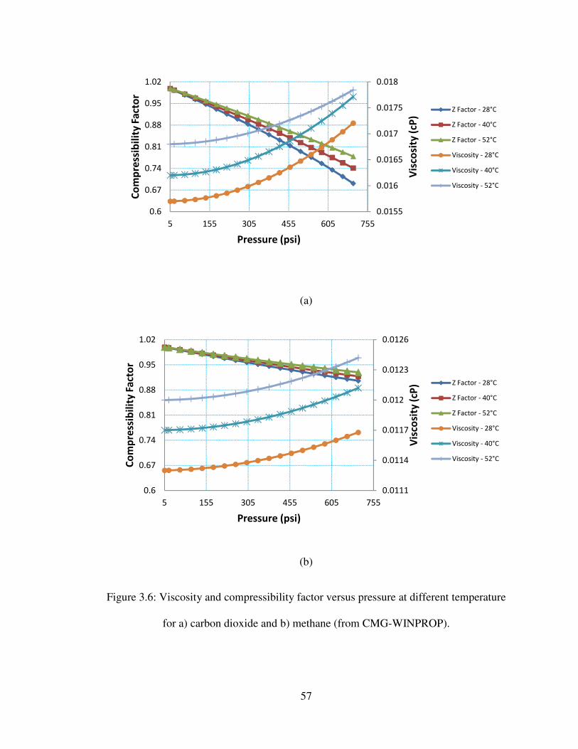
57
(a)
(b)
Figure 3.6: Viscosity and compressibility factor versus pressure at different temperature
for a) carbon dioxide and b) methane (from CMG-WINPROP).
0.0155
0.016
0.0165
0.017
0.0175
0.018
0.6
0.67
0.74
0.81
0.88
0.95
1.02
5 155 305 455 605 755
Vis
cosi
ty (
cP)
Co
mp
ress
ibil
ity
Fa
cto
r
Pressure (psi)
Z Factor - 28°C
Z Factor - 40°C
Z Factor - 52°C
Viscosity - 28°C
Viscosity - 40°C
Viscosity - 52°C
0.0111
0.0114
0.0117
0.012
0.0123
0.0126
0.6
0.67
0.74
0.81
0.88
0.95
1.02
5 155 305 455 605 755
Vis
cosi
ty (
cP)
Co
mp
ress
ibil
ity
Fa
cto
r
Pressure (psi)
Z Factor - 28°C
Z Factor - 40°C
Z Factor - 52°C
Viscosity - 28°C
Viscosity - 40°C
Viscosity - 52°C
58
3.5.2 Two-phase heavy oil / water displacement experiment
The following procedure was carried out for each of the heavy oil / water
displacement experiments using the setup previously shown in Figure (3.1):
• The clean, dried core was first weighed and then placed into the core
holder.
• After applying 750 psi overburden pressure, carbon dioxide gas was
injected at a high rate for one hour to remove any remaining toluene, from
the cleaning process, in the core.
• The desired temperature was set on the temperature controller and the
transfer cylinder was filled with heavy oil and allowed to equilibrate for
24 hours.
• The pressure transducer was calibrated by an ISCO syringe pump at
constant pressure mode.
• The core was vacuumed for two hours and saturated with brine to measure
porosity and to establish the initial conditions of 100% brine saturation.
• Back pressure was maintained by an EQUILIBAR Precision back pressure
regulator (BPR) set to 150 psi.
• The core was aged using 20 PVs of brine at a low rate of 0.05 ml/min to
restore any wettability alteration by miscible cleaning.
• Absolute permeability was measured by brine injection at several different
flow rates.
• Assuring there was no change in the porosity and absolute permeability,
oil was injected at a constant rate of 0.1 ml/min via a transfer cylinder.
59
This rate is equivalent to 1 ft/day of a common flow rate in field scale
waterflooding projects.
• Oil injection was continued until irreducible water saturation was
established.
• During oil injection, effluent fractions were collected in the graduated
tubes while recording time.
• Oil injection was then stopped and the core assembly was given 12 hours
in order to allow the pressure gradient along the core to reach equilibrium.
• In the next phase of the experiment, brine was injected at a constant rate of
0.1 ml/min until residual oil saturation is achieved.
• Graduated test tubes were centrifuged for fractional and recovery analysis.
3.5.3 Two-phase heavy oil / gas displacement experiment
The procedure for two-phase heavy oil / gas displacement experiment is almost
the same as that of a heavy oil / water system, as previously shown in Figure (3.2). A
precise BRONKHORST gas flow controller, given in Figure (A-5), was used to
accurately inject gas (11 mln/min) into the core. A resin-sealed separator, seen in Figure
(A-6), was used to separate liquid effluent from the produced gas. Gas effluent was
passed through a COLE PARMER gas flow meter, seen in Figure (A-7), to record the gas
flow rate out of the core holder.
3.5.4 Three-phase displacement experiment
The idea behind a three-phase displacement experiment is to permit simultaneous
flow of three phases in the porous media over a wide range of saturations. This can be
60
achieved by injecting one phase (gas) into the core saturated with other phases (heavy oil
and water). The following procedure was used to perform a three-phase displacement
experiment:
• The clean, dried core was first weighed and then placed into the core
holder.
• After applying an overburden pressure of 750 psi, carbon dioxide gas was
injected at a high rate for one hour to remove any remaining toluene, from
the cleaning process, in the core.
• The desired temperature was set on the temperature controller and the
transfer cylinder was filled with heavy oil and allowed 24 hours to
equilibrate.
• The pressure transducer was calibrated using an ISCO syringe pump at
constant pressure mode.
• The core was vacuumed for two hours, and saturated with brine to
measure porosity and to establish the initial conditions of 100% brine
saturation.
• Back pressure was maintained by an EQUILIBAR Precision back pressure
regulator (BPR) set to 150 psi.
• The core was aged using 20 PVs of brine at a low rate of 0.05 ml/min to
restore any wettability alteration that may have occurred by miscible
cleaning.
• Absolute permeability was measured by brine injection at several different
flow rates.

61
• Assuring there was no change in the porosity and absolute permeability,
oil was injected at a constant rate of 0.1 ml/min via a transfer cylinder.
This rate is equivalent to 1 ft/day of a common flow rate in field scale
waterflooding projects.
• Effluent fractions were collected in the graduated tubes.
• Oil injection was continued until establishing the desired heavy oil and
water saturation through the core. It should be mentioned that, although, in
other studies (Sarem, 1966) the oil phase injection was stopped
immediately after breakthrough, it was decided to stop oil injection a few
milliliters before breakthrough to allow more water phase remains in the
core.
• Oil injection was then stopped and the core assembly was given 12 hours
to allow the pressure gradient along the core to reach equilibrium.
• In the next phase of the experiment, carbon dioxide was injected via a
HIGH-TECH BRONKHORST gas flow controller at a constant rate of 5
mln/min.
• A COLE PARMER gas flow meter records gas effluent while liquid
fractions were collected in graduated test tubes.
• Graduated test tubes were centrifuged for fractional and recovery analysis.
3.6 Chapter Summary
As this study aims to extensively investigate two- and three-phase relative
permeability data, three different experimental setups were designed to conduct a series

62
of two-phase, three-phase, unsteady state, and steady state experiments. All experiments
were carried out at constant temperature in order to study the effect of temperature on
relative permeabilities. Porous media and fluids were selected that match those of typical
Canadian reservoirs. Regardless of the number of technically failed experiments, 22
successful experiments were performed in this study. Tables (3.2) and (3.3) showcase the
results of each of the tests conducted in this work.
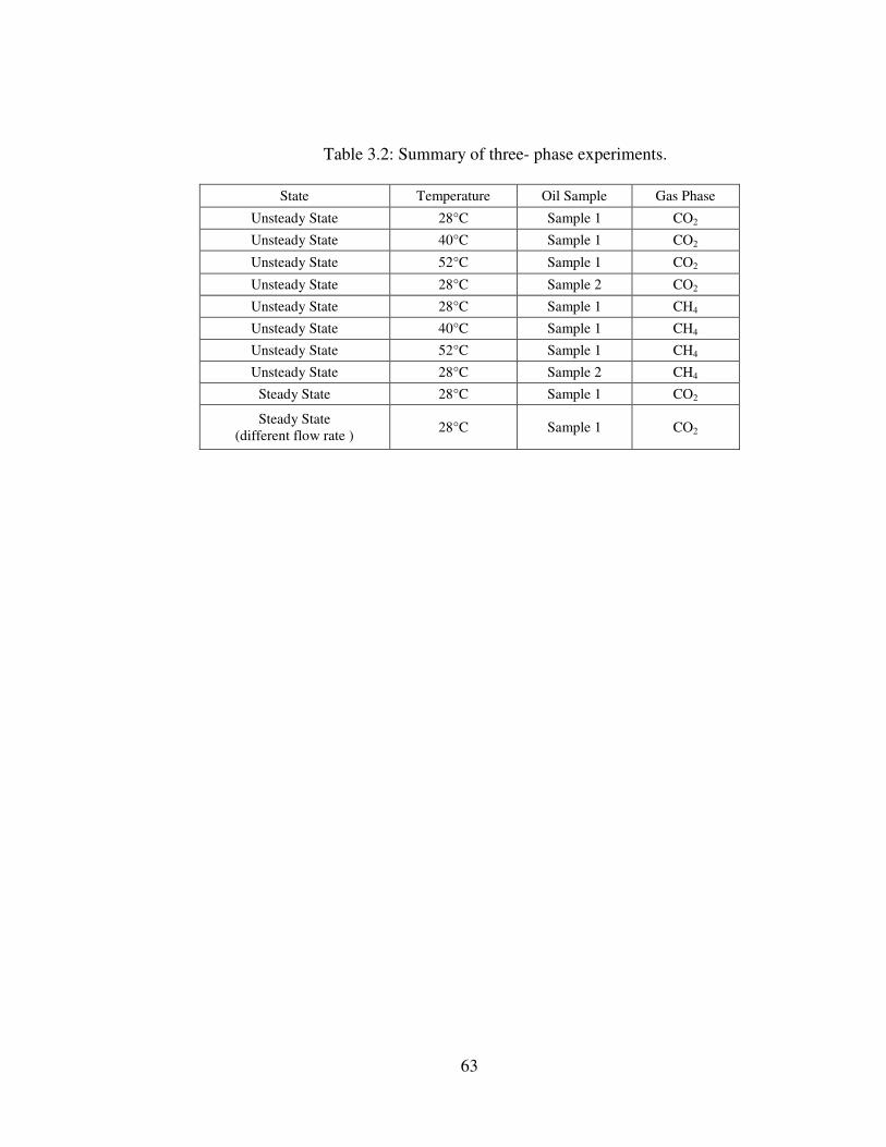
63
Table 3.2: Summary of three- phase experiments.
State Temperature Oil Sample Gas Phase
Unsteady State 28°C Sample 1 CO2
Unsteady State 40°C Sample 1 CO2
Unsteady State 52°C Sample 1 CO2
Unsteady State 28°C Sample 2 CO2
Unsteady State 28°C Sample 1 CH4
Unsteady State 40°C Sample 1 CH4
Unsteady State 52°C Sample 1 CH4
Unsteady State 28°C Sample 2 CH4
Steady State 28°C Sample 1 CO2
Steady State
(different flow rate ) 28°C Sample 1 CO2

64
Table 3.3: Summary of two- phase displacement experiments.
Fluids Temperature Oil Sample
Heavy Oil / Water 28°C Sample 1
Heavy Oil / Water 40°C Sample 1
Heavy Oil / Water 52°C Sample 1
Heavy Oil / Water 28°C Sample 2
Heavy Oil / CO2 28°C Sample 1
Heavy Oil / CO2 40°C Sample 1
Heavy Oil / CO2 52°C Sample 1
Heavy Oil / CO2 28°C Sample 2
Heavy Oil / CH4 28°C Sample 1
Heavy Oil / CH4 40°C Sample 1
Heavy Oil / CH4 52°C Sample 1
Heavy Oil / CH4 28°C Sample 2

65
CHAPTER 4
TWO-PHASE RELATIVE PERMEABILITY WITH JBN
TECHNIQUE
4.1 Introduction
This chapter investigates application of the Johnson-Bossler-Naumann (JBN)
(Johnson, 1959) technique in order to calculate two-phase relative permeabilities using
two-phase displacement experiments. As described in the previous chapter, a series of
two-phase coreflood tests were conducted at different temperatures (28ºC, 40ºC, 52ºC)
and, as well, at different oil viscosities and gas phases (carbon dioxide and methane). The
effects of such parameters on relative permeability curves of heavy oil / water, heavy oil /
carbon dioxide, and heavy oil / methane systems were studied.
4.2 JBN Technique
Although unsteady state relative permeability measurements can be made faster
than steady state measurements, there are more calculations involved in the unsteady-
state technique. The theory was first developed by Buckley and Leverett (1942) and,
later, extended by Weldge (1952) for general use in calculating two-phase relative
permeability under unsteady-state conditions (Amyx et al., 1988). A summary of the JBN
technique for waterflooding process is given below:
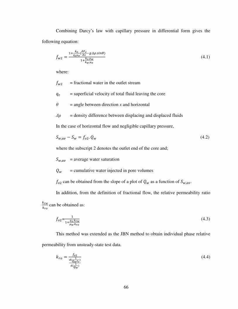
66
Combining Darcy’s law with capillary pressure in differential form gives the
following equation:
2�# = �T 6�9XY�(Z5%ZL ��.∆.�\?])�T6�6�
Y�Y� (4.1)
where:
2�# = fractional water in the outlet stream
=^ = superficial velocity of total fluid leaving the core
θ = angle between direction x and horizontal
∆ρ = density difference between displacing and displaced fluids
In the case of horizontal flow and negligible capillary pressure,
/�,I_ − /� = 2�#. `� (4.2)
where the subscript 2 denotes the outlet end of the core and;
/�,I_ = average water saturation
`� = cumulative water injected in pore volumes
2�#can be obtained from the slope of a plot of `� as a function of /�,I_.
In addition, from the definition of fractional flow, the relative permeability ratio
�!��!� can be obtained as:
2�#=�
�TY�Y�6!�6!�
(4.3)
This method was extended as the JBN method to obtain individual phase relative
permeability from unsteady-state test data.
��� = <�&a( *3�b!)a( *3�)
(4.4)

67
��� = <�&<�&
���� ��� (4.5)
c� = (9�X∆5 )(9�X∆5 )KXQXK!X�dABef%XA�B (4.6)
Where Ir is called relative injectivity.
As an example, feed data for the JBN technique and, also, calculated saturations and
relative permeabilities are presented in Table (4.1) for heavy oil / water at 28ºC.

68
Table 4.1: Relative permeability data calculated by JBN technique at 28ºC for heavy oil
(sample#1)/ water.
Injected
Water
(PV)
Produced Oil
(PV)
Differential
Pressure (Psi)
Water
Saturation
( Fraction)
Water Relative
Permeability
Oil Relative
Permeability
0.502 0.318 43.887
0.834 0.405 18.771 0.354 0.00162 0.12232
0.937 0.425 16.032 0.374 0.00174 0.11720
1.041 0.432 14.346 0.381 0.00183 0.11206
1.263 0.440 13.685 0.386 0.00194 0.09970
1.456 0.456 14.290 0.403 0.00120 0.08990
1.664 0.464 13.041 0.409 0.00211 0.08397
1.871 0.474 12.660 0.418 0.00218 0.07821
2.079 0.476 12.346 0.420 0.00225 0.07337
2.286 0.477 11.881 0.421 0.00233 0.06949
5.493 0.512 10.506 0.449 0.00294 0.04002

69
4.3 Two-Phase Relative Permeabilities Based on JBN Technique
Table (3.3) presents the results of eight successful two-phase displacements
experiment performed at three different temperature (28ºC, 40ºC, 52ºC), using two heavy
oil samples (different viscosity), in the presence of carbon dioxide and methane. With
differential pressure and fractional effluent data, the JBN technique was applied to
calculate heavy oil, water, and gas relative permeabilities. Average saturations were
calculated using the material balance method. Attempts was made to ensure that dead
volumes in the system are as low as possible so as minimize errors in the material balance
calculation. Sample data and, also, detailed procedure of applying JBN technique can be
found in the papers published out of this section (Akhlaghinia et al. 2013-a; Akhlaghinia
et al. 2013-b).
4.3.1 Heavy oil / water systems
The procedure described previously in Sec 3.4.2 was repeated four times at
different temperatures 28ºC, 40ºC, 52ºC, as well as two samples of heavy oils of different
oil viscosity. Figure (4.1) shows the heavy oil and water relative permeability data at
different temperature/oil samples taken by brine injection into sandstone core saturated
with heavy oil at irreducible water saturation.

70
(a) (b)
(c) (d)
Figure 4.1: Heavy oil / water relative permeabilities; a: (T=28°C, Oil#1), b: (T=40°C,
Oil#1), c: (T=52°C, Oil#1), d: (T=28°C, Oil#2).
0
0.04
0.08
0.12
0.16
0
0.08
0.16
0.24
0.32
0.3 0.35 0.4 0.45 0.5
kro
krw
(×1
00
)
Sw
Krw
Kro
0
0.07
0.14
0.21
0.28
0
0.1
0.2
0.3
0.4
0.1 0.2 0.3 0.4 0.5
kro
krw
(×1
00
)
Sw
Krw
Kro
0
0.05
0.1
0.15
0.2
0
0.2
0.4
0.6
0.8
0.3 0.35 0.4 0.45 0.5
kro
krw
(×1
00
)
Sw
Krw
Kro
0
0.13
0.26
0.39
0.52
0
0.04
0.08
0.12
0.16
0.3 0.37 0.44 0.51 0.58
kro
krw
(×1
00
)
Sw
Krw
Kro
krw krw
kro kro
krw
kro
krw
kro

71
Figure (4.2) reveals that temperature has different effects on the water and oil
relative permeability curves. In the case of water relative permeability, the curves shifted
upward by about 66% when temperature ranged between 28ºC to 40ºC. Almost the same
increase is observed for relative permeability curves at 40ºC and 52ºC. With the same
difference between these curves, it can be concluded that temperature linearly increases
the water relative permeability curves. In the case of oil relative permeability curves,
although a 69% increase in relative permeabilities is found between 28ºC to 40ºC, the
relative permeability values decrease by about 32% when temperature ranged between
40ºC to 52°C. It can be concluded that oil relative permeability shifts up until an
optimum temperature before the trend reverses as temperature increases further.
Two heavy oil / water experiments were performed at 28ºC using two different oil
viscosities, with the results given in Figures (4.3-a) and (4.3-b). Heavy oil and water
relative permeabilities were compared in both cases. In contrast to the effect of
temperature on heavy oil / water relative permeabilities, the effect of oil viscosity, as
expected, is found to be such that water relative permeability is inversely proportional to
the oil viscosity for heavy oil / water systems. As one can determine from Figure (4.3-a),
water is more mobile in presence of lighter oil (1174 cP) since relative permeability
values are higher than those in the presence of heavier oil (2658 cP). In contrary, oil
relative permeability is proportional to oil viscosity. This means that oil relative
permeability increases as oil viscosity increases, as shown in Figure (4.3-b).

72
(a)
(b)
Figure 4.2: Effect of temperature on water (a) and heavy oil (b) relative permeabilities.
0
0.001
0.002
0.003
0.004
0.005
0.006
0.007
0.15 0.2 0.25 0.3 0.35 0.4 0.45 0.5
krw
Sw
28°C
40°C
52°C
0
0.05
0.1
0.15
0.2
0.25
0.3
0.15 0.2 0.25 0.3 0.35 0.4 0.45 0.5
kro
Sw
28°C
40°C
52°C

73
(a)
(b)
Figure 4.3: Effect of oil viscosity on water (a) and heavy oil (b) relative permeabilities.
0
0.07
0.14
0.21
0.28
0.35
0.42
0.3 0.35 0.4 0.45 0.5 0.55
kro
Sw
Oil#1 (1174 cP at 28°C)
Oil#2 (2658 cP at 28°C)
0
0.0005
0.001
0.0015
0.002
0.0025
0.003
0.0035
0.3 0.35 0.4 0.45 0.5 0.55
krw
Sw
Oil#1 (1174 cP at 28°C)
Oil#2 (2658 cP at 28°C)

74
4.3.2 Heavy oil / gas systems
The procedure mentioned above for heavy oil / water system was also repeated for
heavy oil / carbon dioxide, with the results given in Figure (4.4), and heavy oil / methane,
with the results given in Figure (4.5). The experimental procedure was previously
described in Sec 3.4.3. The solubility of carbon dioxide and methane in heavy oil was
considered negligible due to the high viscosity of the oil. Also, since gas injections were
performed in short span of time (less than three hours), no sensible solution of gas in the
heavy oil could occur during the experiments allows using the JBN technique to calculate
relative permeabilities. Quantitative measurement of different gas solubility in heavy oil
at different temperature/pressure conditions can be found elsewhere (Tharanivasan et al.,
2006; Etminan, 2009; Marufuzzaman, 2010).
Heavy oil viscosity was routinely measured to ensure that no alteration in heavy
oil viscosity occurs due to the probable vaporization of kerosene during the experiments.
No viscosity change was observed even for the oil produced, indicating that no
considerable mass transfer occurred in the cases of gas injections. Low differential
pressure (up to 5 psi) across the core after breakthrough allowed assuming that both gas
volume and rate do not change considerably in the core. In the case of derivative
calculations, the tangent line passing through each point was taken to be the derivative in
order to avoid the difficulties that had been experienced while fitting the data using
conventional curve fitting techniques,

75
Figure 4.4: Heavy oil / CO2 relative permeabilities; a: (T=28°C, Oil#1), b: (T=40°C,
Oil#1), c: (T=52°C, Oil#1), d: (T=28°C, Oil#2).
0
0.06
0.12
0.18
0.24
0
0.07
0.14
0.21
0.28
0.74 0.77 0.8 0.83 0.86
krg
(×1
00
00
)
kro
So
Kro
Krg
0
0.1
0.2
0.3
0.4
0
0.05
0.1
0.15
0.2
0.72 0.75 0.78 0.81 0.84
krg
(×1
00
00
)
kro
So
Kro
Krg
0
0.3
0.6
0.9
1.2
0
0.07
0.14
0.21
0.28
0.72 0.78 0.84 0.9 0.96
krg
(×1
00
00
)
kro
So
Kro
Krg
0
0.05
0.1
0.15
0.2
0
0.04
0.08
0.12
0.16
0.3 0.44 0.58 0.72 0.86
krg
(×1
00
00
)
kro
So
Kro
Krg
(a) (b)
(c) (d)
kro
krg
kro
krg
kro
krg
kro
krg

76
Figure 4.5: Heavy oil / CH4 relative permeabilities; a: (T=28°C, Oil#1), b: (T=40°C,
Oil#1), c: (T=52°C, Oil#1), d: (T=28°C, Oil#2).
0
0.08
0.16
0.24
0.32
0
0.015
0.03
0.045
0.06
0.55 0.62 0.69 0.76 0.83
krg
(×1
00
00
)
kro
So
Kro
Krg
0
0.08
0.16
0.24
0.32
0
0.005
0.01
0.015
0.02
0.67 0.705 0.74 0.775 0.81
krg
(×1
00
00
)
kro
So
Kro
Krg
0
0.25
0.5
0.75
1
0
0.04
0.08
0.12
0.16
0.55 0.62 0.69 0.76 0.83
krg
(×1
00
00
)
kro
So
Kro
Krg
0
0.025
0.05
0.075
0.1
0
0.06
0.12
0.18
0.24
0.65 0.71 0.77 0.83 0.89
krg
(×1
00
00
)
kro
So
Kro
Krg
(a) (b)
(c) (d)
kro
krg
kro
krg
kro
krg
kro
krg

77
Figure (4.6) presents the results of applying the JBN technique to heavy oil /
methane and heavy oil / carbon dioxide systems. The effect of increase in temperature on
both methane and carbon dioxide relative permeabilities are the same as those for water.
Figures (4.6-b) and (4.6-d) indicate that as temperature increases from 28ºC to 52ºC,
methane and carbon dioxide relative permeabilities increase. Unexpectedly, heavy oil
relative permeability in presence of methane tends to decrease from 28ºC to 40ºC and
then, as temperature further increases, it dramatically increases. This phenomenon is seen
in Figure (4.6-a). This graph indicates a reversal trend of the heavy oil relative
permeability by the temperature. In the case of oil relative permeability in presence of
carbon dioxide, it is seen to fall as temperature climbs. This is observed in Figure (4.6-c).
The effect of oil viscosity on relative permeabilities of heavy oil / methane and
heavy oil / carbon dioxide was also investigated in this study. Figure (4.7) shows that the
effect of oil viscosity of heavy oil and gas (carbon dioxide and methane) relative
permeabilities is exactly the same as that previously observed for heavy oil / water
system. Methane, as one can see from Figure (4.7-b), and carbon dioxide, as Figure (4.7-
d) shows, relative permeabilities are inversely proportional to the oil viscosity of heavy
oil / gas systems. Oil relative permeability is proportional to oil viscosity such that it
increases as oil viscosity increases. This is seen in Figures (4.7-a) and (4.7-b).

78
Figure 4.6: Effect of temperature on heavy oil / gas relative permeabilities; a and b (CH4),
c and d (CO2).
0
0.04
0.08
0.12
0.16
0.55 0.61 0.67 0.73 0.79 0.85
kro
So
28°C
40°C
52°C
0
0.2
0.4
0.6
0.8
1
0.55 0.6 0.65 0.7 0.75 0.8
krg
(×1
00
00
)
So
28°C40°C
52°C
0
0.07
0.14
0.21
0.28
0.72 0.77 0.82 0.87 0.92 0.97
kro
So
28°C
40°C
52°C0
0.3
0.6
0.9
1.2
0.72 0.775 0.83 0.885 0.94 0.995
krg
(×1
00
00
)
So
28°C
40°C
52°C
(a) (b)
(c) (d)
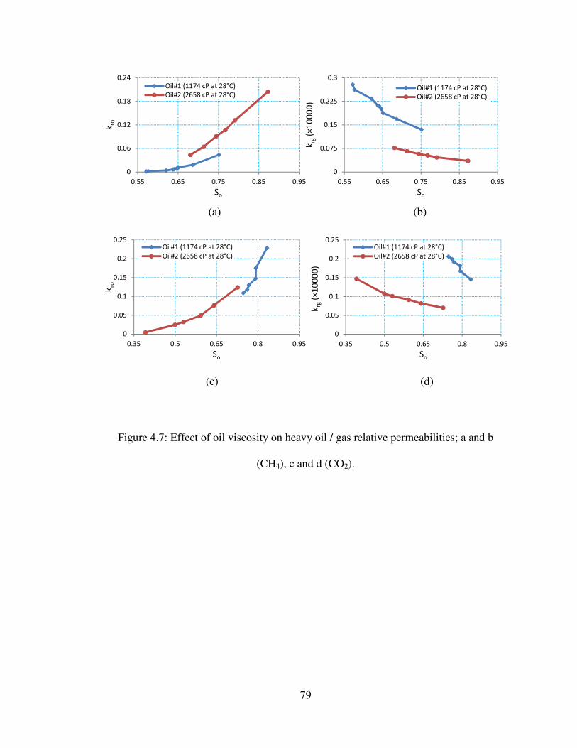
79
Figure 4.7: Effect of oil viscosity on heavy oil / gas relative permeabilities; a and b
(CH4), c and d (CO2).
(a) (b)
(c) (d)
0
0.06
0.12
0.18
0.24
0.55 0.65 0.75 0.85 0.95
kro
So
Oil#1 (1174 cP at 28°C)
Oil#2 (2658 cP at 28°C)
0
0.075
0.15
0.225
0.3
0.55 0.65 0.75 0.85 0.95
krg
(×1
00
00
)
So
Oil#1 (1174 cP at 28°C)
Oil#2 (2658 cP at 28°C)
0
0.05
0.1
0.15
0.2
0.25
0.35 0.5 0.65 0.8 0.95
kro
So
Oil#1 (1174 cP at 28°C)
Oil#2 (2658 cP at 28°C)
0
0.05
0.1
0.15
0.2
0.25
0.35 0.5 0.65 0.8 0.95
krg
(×1
00
00
)
So
Oil#1 (1174 cP at 28°C)
Oil#2 (2658 cP at 28°C)

80
4.4 Chapter Summary
Two-phase unsteady state experiments were performed in order to measure heavy
oil-water, heavy oil carbon dioxide, and heavy oil-methane relative permeabilities. Using
fractional effluents measured with precision meters and differential pressure data records,
the JBN technique was applied to calculate two-phase relative permeability in a
consolidated sandstone core. A series of coreflood tests were conducted at three different
temperatures (28ºC, 40ºC, and 52ºC) and using two oil samples of different viscosities.
Analysis of the data obtained for heavy oil-water system show a linear increase of about
65% and 50% in water relative permeabilities when temperature ranged 28ºC to 40ºC and
40ºC to 52ºC, respectively. However, while the oil relative permeability curve shows an
increase of about 70% when temperature increases from 28ºC to 40ºC, it dramatically
falls by about 30%, when temperature rises from 40ºC to 52ºC. Both methane and carbon
dioxide relative permeabilities increase non-linearly at higher temperatures. Oil relative
permeability in presence of carbon dioxide decreases when temperature increases. In
contrast, in presence of methane, oil relative permeability experiences a reduction of 80%
from 28ºC to 40ºC, followed by a considerable increase of fifteenfold from 40ºC to 52ºC.
The effect of oil viscosity for all three systems was observed to be the same. Methane,
carbon dioxide, and water relative permeabilities are inversely proportional to the oil
viscosity. On the other hand, oil relative permeability tends to increase as its viscosity
increases. A summary of the results obtained in this chapter is presented in Tables (4.2)
and (4.3). Also, detailed discussion on the applicability of JBN technique for heavy oil
systems can be found in the papers published out of this chapter (Akhlaghinia et al. 2013-
a; Akhlaghinia et al. 2013-b).

81
Table 4.2: Summary of effect of increase in temperature on the relative permeability of
two-phase systems.
krw krg kro
Heavy Oil-Water Increase ----- Increase/Decrease
Heavy Oil-Carbon Dioxide ----- Increase Decrease
Heavy Oil-Methane ----- Increase Decrease/Increase

82
Table 4.3: Summary of effect of increase in oil viscosity on the relative permeability of
two-phase systems.
krw krg kro
Heavy Oil-Water Decrease ----- Increase
Heavy Oil-Carbon Dioxide ----- Decrease Increase
Heavy Oil-Methane ----- Decrease Increase

83
CHAPTER 5
THREE-PHASE RELATIVE PERMEABILITY ISOPERMS
5.1 Introduction
With a three-phase displacement experiment, it is possible to have simultaneous
flow of three phases in the porous media over a wide range of saturations. This condition
cannot be achieved in the steady state experiment since saturation is homogenous and
constant in the porous medium while all phases flow at steady rates through that medium.
In this chapter, a technique is brought forward to generate relative permeability isoperms
(for three-phase systems) using a three-phase displacement experiment that involves
injecting gas into Berea consolidated core saturated with heavy oil and water. After
validating this technique, the effects of parameters such as temperature, oil viscosity, and
gas phase on the relative permeability isoperms are investigated. The highlights of this
chapter include:
• Proposing a technique to generate three-phase relative permeability
isoperms based on two- and three-phase displacement experiments
combined with a suitable lab-scale simulator.
• Validation of the generated three-phase relative permeability isoperms by
comparing the findings with results obtained from the steady state
experiment and, also, through conducting a sensitivity analysis.

84
• Investigating of the effect of temperature, oil viscosity, and different gas
phase on the three-phase relative permeability isoperms.
5.2 Procedure
An algorithm was constructed to utilize two- and three-phase unsteady state
displacements in order to estimate the relative permeability isoperms of a fluid system of
heavy oil / water / gas. The four main elements of this algorithm are:
• Two-phase displacement experiment as needed to determine the
boundaries of the relative permeability isoperms.
• Three-phase displacement experiment.
• Three-phase simulator able to handle three-phase relative permeabilities in
explicit form.
• A tool to plot isoperms/contours using generated relative permeability
data.
Using residual oil saturation (Sor) and irreducible water saturation (Swi) obtained
from two-phase heavy oil / water floods, a three-phase flow zone in a ternary diagram
was assigned. Three-phase displacement was conducted in the form of gas injection into a
consolidated Berea core saturated with heavy oil and water. A three-phase lab scale
simulator was developed to simulate a three-phase displacement experiment. Appropriate
three-phase relative permeability data was selected that corresponds to a saturation path
drawn across the three-phase flow zone in the ternary diagram (e. g., saturation path 1, 2,
and 3 in Figure (5.1)). This relative permeability data was continuously fine-tuned until
differential pressure, heavy oil production, and water production from the numerical
simulator match those of the three-phase displacement experiment. Repeating this

85
procedure for different saturation paths leads to a set of relative permeability data that can
be used to plot isoperms/contours in a ternary diagram. Figure (5.1) presents a typical
three-phase flow zone of the heavy oil / water / gas system. This entire procedure is
visualized in a flowchart in Figure (5.2).
5.3 Determination of Three-Phase Flow Zone
Leverett and Lewis (1941) introduced the concept of the three-phase flow zone in
a ternary diagram. They proposed that, while ignoring the irreducible gas saturation Sgi,
the saturation region is one in which simultaneous flow of all three phases is limited by
irreducible water saturation Swi, and residual oil saturation Sor. Figure (5.3) presents a
typical three-phase flow zone of the heavy oil / water / gas.
Irreducible water saturation Swi, and residual oil saturation Sor used in this chapter
were found using the heavy oil / water displacement experiments described in Sec 4.3.1
at three different temperatures and two different oil viscosities. Figure (5.4) and Figure
(5.5) indicate how oil and water saturation changed until irreducible water saturation and
residual oil saturation were achieved. Note that the average saturation calculated by
material balance was used in this study.
Results show that increasing temperature tends to make Berea core more water
wet, since irreducible water saturation increases at higher temperatures. In contrast,
residual oil saturation decreases as temperature increases. In addition, it can be observed
that oil flooding with more viscous oil results in lower irreducible water saturation,
because the process is more piston-like. A summary of test the conditions and, as well as
the established irreducible water saturation (Swi) and residual oil saturation (Sor) are
presented in Table (5.1).

Figure 5.1: Saturation path selection through the three
86
Figure 5.1: Saturation path selection through the three-phase zone (original
(original in color).

87
Figure 5.2: Procedure used to estimate three-phase relative permeability data from
unsteady state displacement experiments.

Figure 5.3: Typical three
88
hree-phase flow zone for heavy oil/water/gas system
color).
phase flow zone for heavy oil/water/gas system (original in

89
Figure 5.4: Average water saturation change during oil injection.
0
0.2
0.4
0.6
0.8
1
1.2
0 1 2 3 4 5 6 7
Sw
(Fra
ctio
n)
Injected Oil (PV)
Case#1
Case#2
Case#3
Case#4

90
Figure 5.5: Average oil saturation change during water injection.
0
0.2
0.4
0.6
0.8
1
1.2
0 1 2 3 4 5 6 7
So
(Fra
ctio
n)
Injected Water (PV)
Case#1
Case#2
Case#3
Case#4
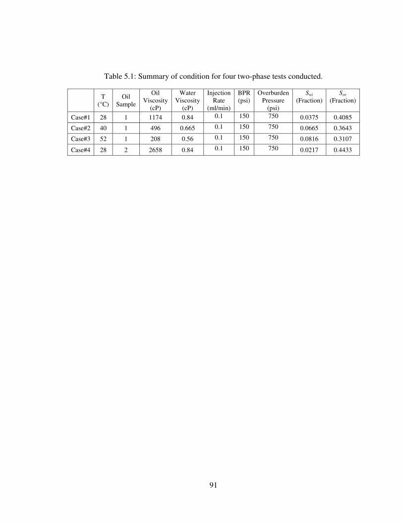
91
Table 5.1: Summary of condition for four two-phase tests conducted.
T
(°C)
Oil
Sample
Oil
Viscosity
(cP)
Water
Viscosity
(cP)
Injection
Rate
(ml/min)
BPR
(psi)
Overburden
Pressure
(psi)
Swi
(Fraction)
Sor
(Fraction)
Case#1 28 1 1174 0.84 0.1 150 750 0.0375 0.4085
Case#2 40 1 496 0.665 0.1 150 750 0.0665 0.3643
Case#3 52 1 208 0.56 0.1 150 750 0.0816 0.3107
Case#4 28 2 2658 0.84 0.1 150 750 0.0217 0.4433

92
5.4 Three-Phase Displacement Experiments
As mentioned earlier, a three-phase displacement experiment allows simultaneous
flow of three phases in a porous medium over a wide range of saturations. On the
contrary, each steady state experiment provides a single relative permeability data point
in a ternary diagram. In this study, three-phase displacement experiments were conducted
involving gas (carbon dioxide, methane) injection into a consolidated Berea core at fixed
heavy oil and water saturations. Preparations for this test are the same as those described
for two-phase displacement. It is desirable to achieve two-phase saturation in the core
before gas injection. In the unsteady state experiments conducted by Sarem (1966), oil
injection into the core 100% saturated with brine was stopped immediately after
breakthrough. In this study, oil injection is halted few milliliters before breakthrough as
to guarantee that more water phase remains in the core. After establishing two-phase
saturation in the core (e.g. Sw = 0.30, So = 0.70), the core assembly was given 12 hours to
enable the pressure gradient along the core to reach equilibrium. In the next phase, gas
was injected via a BRONKHORST gas flow controller at constant rate of 5 mln/min. A
COLE PARMER gas flow meter recorded gas effluent, while liquid fractions were
collected in the graduated test tubes (details of the experimental procedure previously
described in Sec 3.4.4). In total, 8 successful three-phase displacement experiments at
different temperatures, oil viscosities, and gas phase were conducted in this study. Oil
and water saturations established before gas injection are presented in Table (5.2). As a
base case, Figure (5.6) presents pressure drop, water production, and oil production
observed during the carbon dioxide injection process (initially saturated with 30% water
and 70% heavy oil). Similar plots for the rest of tests are found in Appendix B.

93
Table 5.2: Oil and water saturations before gas injections.
Gas Temperature
(°C)
Oil
Sample
Oil
Viscosity
(cP)
Water
Viscosity
(cP)
Sw
(Fraction)
So
(Fraction)
Test#1 CO2 28 1 1174 0.84 0.30 0.70
Test#2 CO2 40 1 496 0.665 0.28 0.72
Test#3 CO2 52 1 208 0.56 0.28 0.72
Test#4 CO2 28 2 2658 0.84 0.29 0.71
Test#5 CH4 28 1 1174 0.84 0.29 0.71
Test#6 CH4 40 1 496 0.665 0.29 0.71
Test#7 CH4 52 1 208 0.56 0.30 0.70
Test#8 CH4 28 2 2658 0.84 0.29 0.71

94
Figure 5.6: Results from three-phase displacement for base case (carbon dioxide injection
at 28°C).
0
10
20
30
40
50
60
70
0
0.02
0.04
0.06
0.08
0.1
0.12
0 200 400 600 800 1000
Pre
ssu
re D
rop
(p
si)
Pro
du
ctio
n (
PV
)
Time(min)
Oil Production
Water Production
Pressure Drop

95
5.5 Numerical Simulation
The algorithm employed in this study for the estimation of the three-phase relative
permeability isoperms requires a numerical simulation of the three-phase displacement
experiments. Unlike commercial numerical simulators, such as CMG and ECLIPSE,
which use probabilistic models based on two-phase relative permeability data, the
numerical simulator developed in this study can use explicit three-phase permeability
data.
A one-dimensional three-phase numerical simulator was developed that used a
continuity equation for the immiscible flow of each phase through porous media, one that
includes the Darcy equation as a momentum term. These equations were solved by an
implicit technique as to eliminate any uncertainty in the numerical modeling. Details of
the procedure are given in Appendix C. The MATLAB code of the simulator is found in
Appendix D.
Before using the lab scale simulator to simulate a three-phase displacement
experiment, its integrity needed to be validated. To do so, a generic, one-dimensional, and
three-phase model was utilized to compare this simulator with CMG-IMEX simulator.
Details of the generated model, including initial condition, dimension, rock/fluid
properties, and injector/producer constraints, are presented in Table (5.3). Figure (5.7)
shows oil / water and liquid / gas relative permeability curves used in both the developed
simulator and CMG-IMEX to simulate carbon dioxide injection at a constant rate into a
model saturated with 63.29% oil, 30.2% water, and 6.51% carbon dioxide. Figure (5.8)
shows acceptable agreement between results (injection pressure, oil production, and
water production) from developed simulator and CMG-IMEX.

96
Table 5.3: Details of the model used to validate developed simulator with CMG-IMEX.
Total Bulk Reservoir Volume cc 962.29
Total Pore Volume cc 187.29
Total Hydrocarbon Pore Volume cc 131.10
Original Oil in Place, OOIP cc 118.53
Original Gas in Place, OGIP cc 3236.59
Original Water in Place, OWIP cc 56.56
Porosity % 19.46
Initial Oil Saturation % 63.29
Initial Gas Saturation % 6.51
Initial Water Saturation % 30.2
Absolute Permeability md 1560
Temperature °F 186
Water Viscosity cP 0.45
Oil Viscosity cP 0.8
Grids No. 50×1×1
I Dimension ft 50×0.0573228
J Dimension ft 1×0.108888
K Dimension ft 1×0.108888
Injector Constraint
CO2 Injection Rate (MAX) ft3/day 0.00847552
Bottom Hole Pressure (MAX) psi 4000
Producer Constraint
Bottom Hole Pressure (MIN) psi 515

97
(a)
(b)
Figure 5.7: Relative permeability data used to validate developed simulator with CMG-
IMEX; a: oil/water relative permeability, b: liquid/gas relative permeability.
0
0.05
0.1
0.15
0.2
0.25
0.3
0.35
0.2 0.3 0.4 0.5 0.6 0.7 0.8
kr
Sw
Krw
Krow
0
0.05
0.1
0.15
0.2
0.25
0.3
0.35
0.5 0.6 0.7 0.8 0.9 1 1.1
kr
Sl
Krg
Krog
krw
krow
krw
krog

98
(a)
(b)
(c)
Figure 5.8: Comparing results from generated simulator with CMG-IMEX using a generic model.
514.9
515
515.1
515.2
515.3
515.4
515.5
515.6
0 1 2 3 4 5 6
Inje
ctio
n
Pre
sssu
re(p
si)
Time (Days)
Simulator
CMG-IMEX
0
20
40
60
80
100
120
0 1 2 3 4 5 6
Oil
Pro
d.
(CC
)
Time (Days)
Simulator
CMG-IMEX
0
0.01
0.02
0.03
0.04
0.05
0.06
0 1 2 3 4 5 6
Wa
ter
Pro
d.
(CC
)
Time (Days)
Simulator
CMG-IMEX

99
5.6 Three-Phase Relative Permeability Isoperms (Base Case)
After validation of the lab scale simulator, it was used to simulate three-phase
displacement experiments. As a base case, results from Test#1 (see Table (5.2)) are
presented in this section. Results for the rest of the tests will be presented in the next and
focus on the effects of temperature, oil viscosity, and gas phase on the relative
permeability isoperms. As shown in the flowchart of Figure (5.2), pressure drop, oil
production, and water production observed from the three-phase displacement experiment
are matched to those predicted by the developed simulator. This procedure was performed
using three sets of relative permeability data (corresponding to three saturation paths
across a three-phase flow zone) to obtain data points in the three-phase flow zone for
plotting isoperms/contours. Figures (5.9), (5.10), and (5.11) showcase the results of three
saturation paths shown in Figure (5.1).

100
Figure 5.9: Results from matching test#1 for saturation path # 1, top (pressure drop),
middle (oil production), and bottom (water production).
0
10
20
30
40
50
60
70
0 100 200 300 400 500 600 700 800 900 1000
ΔP
(p
si)
Time(min)
Experiment
Simulation
0
0.02
0.04
0.06
0.08
0.1
0.12
0 100 200 300 400 500 600 700 800 900 1000
Oil
Pro
d.
(PV
)
Time(min)
Simulation
Experiment
0
0.01
0.02
0.03
0.04
0 100 200 300 400 500 600 700 800 900 1000
Wa
ter
Pro
d.
(PV
)
Time(min)
Simulation
Experiment

101
Figure 5.10: Results from matching test#1 for saturation path # 2, top (pressure drop),
middle (oil production), and bottom (water production)
0
10
20
30
40
50
60
70
0 100 200 300 400 500 600 700 800 900 1000
ΔP
(p
si)
Time(min)
Experiment
Simulation
0
0.02
0.04
0.06
0.08
0.1
0.12
0 100 200 300 400 500 600 700 800 900 1000
Oil
Pro
d.
(PV
)
Time(min)
Simulation
Experiment
0
0.01
0.02
0.03
0.04
0 100 200 300 400 500 600 700 800 900 1000
Wa
ter
Pro
d.
(PV
)
Time(min)
Simulation
Experiment
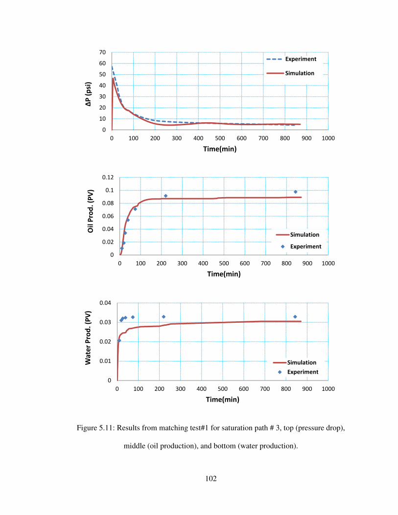
102
Figure 5.11: Results from matching test#1 for saturation path # 3, top (pressure drop),
middle (oil production), and bottom (water production).
0
10
20
30
40
50
60
70
0 100 200 300 400 500 600 700 800 900 1000
ΔP
(p
si)
Time(min)
Experiment
Simulation
0
0.02
0.04
0.06
0.08
0.1
0.12
0 100 200 300 400 500 600 700 800 900 1000
Oil
Pro
d.
(PV
)
Time(min)
Simulation
Experiment
0
0.01
0.02
0.03
0.04
0 100 200 300 400 500 600 700 800 900 1000
Wa
ter
Pro
d.
(PV
)
Time(min)
Simulation
Experiment

103
Final relative permeability isoperms of heavy oil / water / carbon dioxide are
presented in Figures (5.12), (5.13), and (5.14) for oil, water, and carbon dioxide,
respectively. User-friendly software was specially developed for this purpose (see
Appendix E). For convenience, heavy oil, water, gas relative permeability isoperms are
plotted in red, blue, and orange, respectively. Ternary diagrams including in this segment
indicate that the three–phase flow zone is quite small for the heavy oil system due to high
values of residual oil saturation (Sor = 40.85%). Although curvature is observed for all
phases, the curvatures of the various phases are completely different. In the case of oil,
the curvature is more complex than that of water or carbon dioxide. Oil relative
permeability values are higher than those of water and carbon dioxide by an order of
magnitude of three and five, respectively. This difference coincides with the difference
between viscosity of the phases (heavy oil = 1174 cP, water = 0.84 cP, carbon dioxide =
0.015).

Figure 5.12: Oil relative permeability isoperms from test#1
104
elative permeability isoperms from test#1 (original in color)
(original in color).
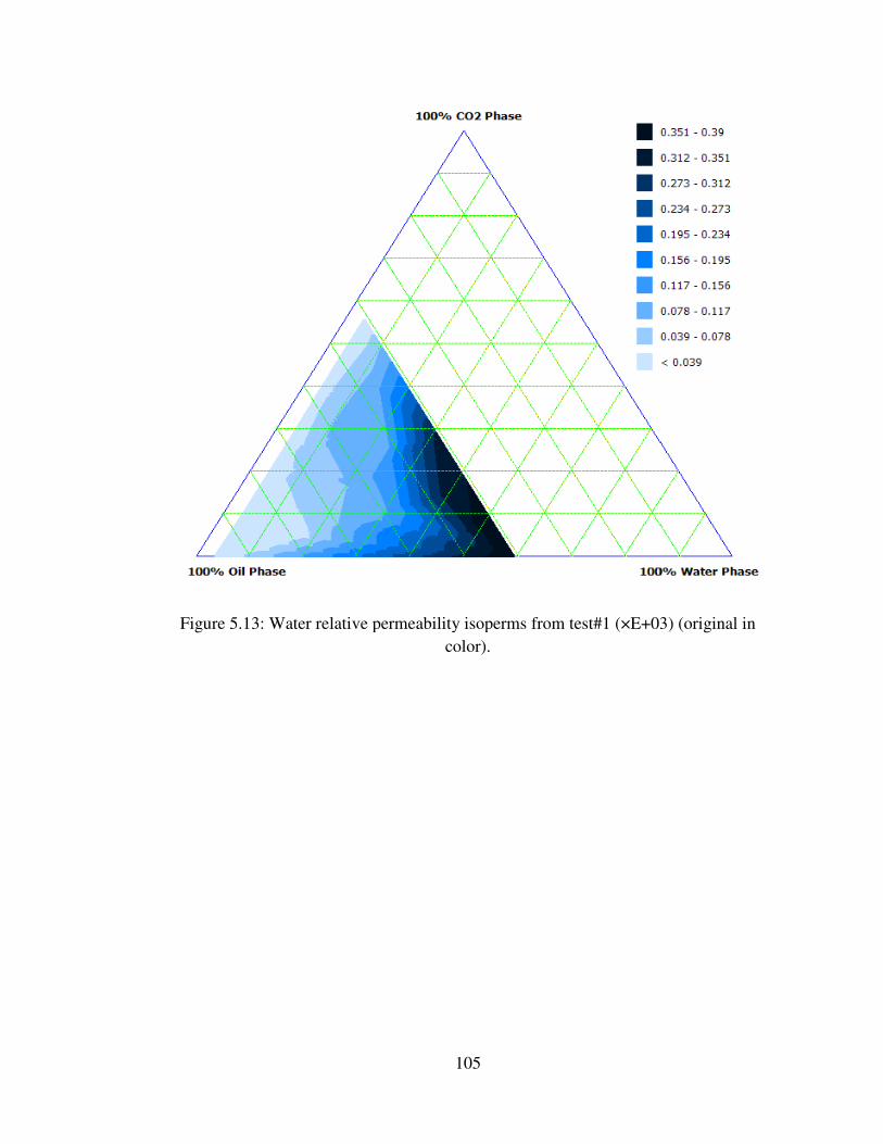
Figure 5.13: Water relative permeability isoperms from test#1
105
elative permeability isoperms from test#1 (×E+03)
color).
(×E+03) (original in

Figure 5.14: Carbon dioxide r
106
Carbon dioxide relative permeability isoperms from test#1 (×E+05)
in color).
(×E+05) (original

107
5.6.1 Validation of the results steady state experiments
In this section, the estimated relative permeabilities obtained previously are
validated using a steady state experiment. The experimental setup shown in Figure (3.3)
was used to simultaneously inject heavy oil, water and carbon dioxide into Berea core.
Check valves were employed at the inlets to prevent back flow. After several failed
attempts, an optimal procedure to reach and maintain simultaneous three-phase flow of
heavy oil, water, and carbon dioxide was found. It is given as follows:
• Core was saturated 100% with water (brine).
• Heavy oil was injected at desired constant rate constant rate.
• After injection of heavy oil, with at least 1.5 pore volumes, water was also
injected at constant rate, much higher than what was desired.
• After reaching an almost simultaneous flow of water and heavy oil, water
flow rate was lowered to desired flow rate.
• Next, carbon dioxide was injected, again, at a flow rate higher than what
was desired.
• After reaching simultaneous flow of heavy oil, water, and carbon dioxide,
gas flow rate was lowered to desired flow rate
• Effluents were repeatedly taken, centrifuged, and read until no change in
the flow rate out of the core (for each phase) is observed.
• Differential pressure and flow rates were then used to calculate relative
permeability and saturations by the way of the following equations:
��� = − g���1�h∆ (5.1)

108
��� = − g���1�h∆ (5.2)
��� = − g���1�h∆ (5.3)
Note that capillary pressure was ignored as it implies that the differential pressure
of all phases is the same. This, in turn, allows one to use Equations (5.1) to (5.3) to
calculate relative permeability of each phase.
After establishing a steady state flow of heavy oil, water, and carbon dioxide in
the core, saturation of the core was next calculated volumetrically using flow rates:
/� = g�g�Tg�Tg� (5.4)
/� = g�g�Tg�Tg� (5.5)
/� = g�g�Tg�Tg� (5.6)
Table (5.4) presents the results of two successful steady state expedites conducted
in order to verify the estimated relative permeabilities obtained by the base case. Figures
(5.15), (5.16), and (5.17) show that the relative permeabilities obtained from the steady
state tests are in good agreement with isoperms previously obtained in base case.
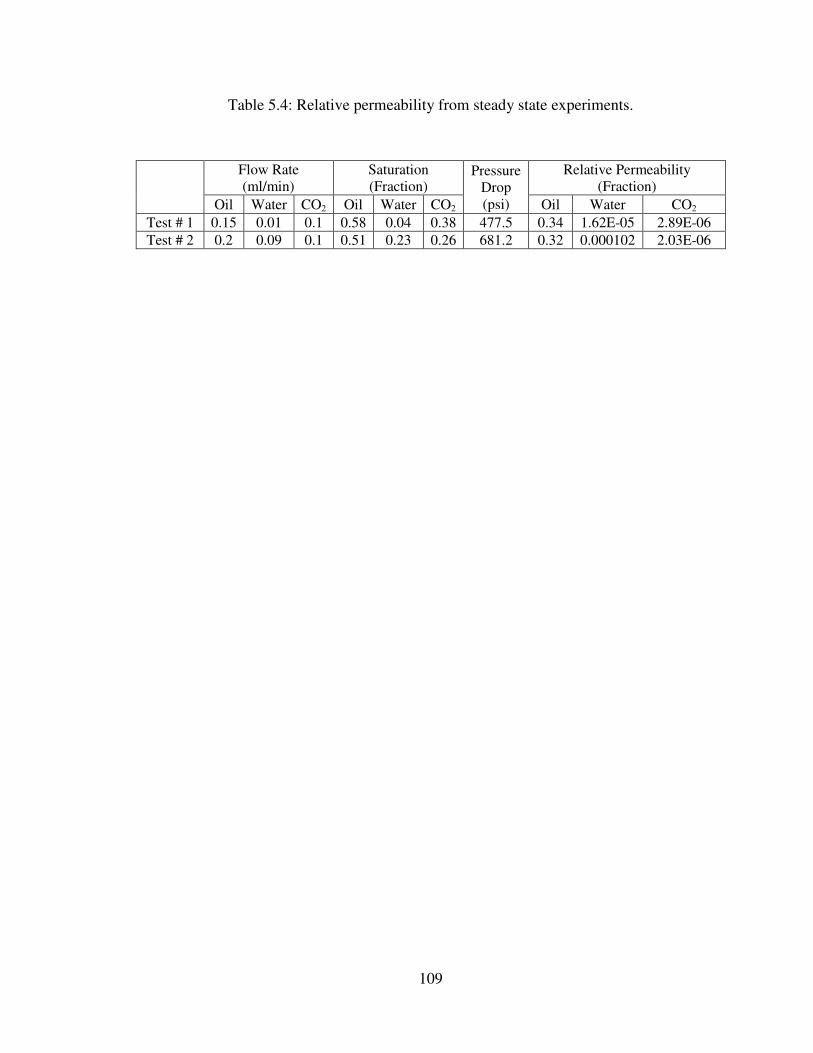
109
Table 5.4: Relative permeability from steady state experiments.
Flow Rate
(ml/min)
Saturation
(Fraction) Pressure
Drop
(psi)
Relative Permeability
(Fraction)
Oil Water CO2 Oil Water CO2 Oil Water CO2
Test # 1 0.15 0.01 0.1 0.58 0.04 0.38 477.5 0.34 1.62E-05 2.89E-06
Test # 2 0.2 0.09 0.1 0.51 0.23 0.26 681.2 0.32 0.000102 2.03E-06

110
Figure 5.15: Validation of oil relative permeability isoperms with steady state tests
(original in color).

111
Figure 5.16: Validation of water relative permeability isoperms with steady state tests
(×E+03) (original in color).

112
Figure 5.17: Validation of gas relative permeability isoperms with steady state tests
(×E+05) (original in color).
113
5.6.2 Sensitivity analysis
A sensitivity analysis was also performed. It examines how manipulation of the
estimated relative permeability data changes the results predicted by the numerical
simulation. As one can see from Figures (5.18), (5.19), and (5.20), there is noticeable
disagreement between the pressure drop simulated using the developed numerical
simulator in comparison to the observation obtained from the three-phase displacement
experiment. It is further inferred that the numerical simulation is more sensitive to gas
relative permeability data in comparison to water and oil relative permeabilities, since
more deviation occurs in simulation results, which used manipulated gas relative
permeability data.

114
Figure 5.18: Effect of change in oil relative permeability data on the pressure drop
predicted by the numerical simulator.
0
10
20
30
40
50
60
70
0 100 200 300 400 500 600 700 800 900
ΔP
(p
si)
Time(min)
Experiment
Kro/2
Matched Kro
Kro/4
Experiment
kro/2
Matched kro
kro/4

115
Figure 5.19: Effect of change in water relative permeability data on the pressure drop
predicted by the numerical simulator.
0
10
20
30
40
50
60
70
0 100 200 300 400 500 600 700 800 900
ΔP
(p
si)
Time(min)
Experiment
Krw/8
Matched Krw
Krw*2
Experiment
krw/8
Matched krw
Krw*2

116
Figure 5.20: Effect of change in CO2 relative permeability data on the pressure drop
predicted by the numerical simulator.
0
10
20
30
40
50
60
70
80
0 100 200 300 400 500 600 700 800 900
ΔP
(p
si)
Time(min)
Experiment
Krg/2
Matched Krg
Krg*10
Experiment
krg/2
Matched krg
Krg*10

117
5.7 Chapter Summary
The three-phase flow zone was determined in a ternary diagram using residual oil
and irreducible water saturations obtained from two-phase heavy oil / water floods. A
fully implicit three-phase simulator was developed to simulate a three-phase
displacement experiment involving gas injection into a consolidated Berea core saturated
with heavy oil and water. Three-phase relative permeability data corresponding to a
saturation path, drawn across the three-phase flow zone in a ternary diagram, was tuned
to match the simulated pressure drop, oil and water production with those observed in the
displacement experiment. Results were then verified using three-phase steady state
experiments and a sensitivity analysis. It has been established that, due to high values of
residual oil saturation, a limited three-phase flow zone exists for heavy oil fluid systems.
Different curvatures were observed for each of the phases. In the case of oil and water,
these curvatures are more complex in comparison to those of carbon dioxide. It has been
concluded that, due to significant viscosity contrast, oil relative permeability values are
higher than those of water and carbon dioxide by an order of magnitude of three and five,
respectively.
118
CHAPTER 6
EFFECT OF TEMPERATURE, OIL VISCOSITY, AND GAS PHASE ON
RELATIVE PERMEABILITY ISOPERMS
6.1 Introduction
In the previous chapter, three-phase relative permeability isoperms were estimated
as a base case for a heavy oil / water / carbon dioxide system at 28°C. Results were
validated using both steady state experiments and a sensitivity analysis. In this chapter,
results of a series of tests at different temperatures, oil viscosities, and gas phases are
presented to:
• Investigate the effect of temperature on relative permeability isoperms
• Investigate the effect of oil viscosity on relative permeability isoperms
• Examine the relative permeability isoperms in the presence of carbon
dioxide and methane
In this section, the final three-phase relative permeability isoperms (for different
temperature conditions, etc.) obtained using the procedure described in the previous
chapter are presented. The results of matching these three-phase displacement
experiments using the developed simulator are detailed in Appendix F.
6.2 Effect of Temperature on Three-phase Relative Permeabilities
In Figures (6.1) and (6.2), relative permeabilities of three phases of a fluid system
of heavy oil / water / gas taken at three temperature, specifically of 28°C, 40°C, and
52°C, are shown side by side. Comparing ternary diagrams, it can be seen that the

119
position of the three-phase flow zone shifts to the right as the temperature increases. This
is due to the opposite effect of temperature on the water irreducible saturation and
residual oil saturation (see Table 5.1). As the temperature rises from 28°C to 52°C,
irreducible water saturation increases from 0.038 to 0.08. On the contrary, increasing the
temperature reduces oil residual saturation from 0.41 to 0.31. This opposite effect causes
the three-phase flow zone to move toward the water vertex, while the size of three-flow
zone does not change significantly.
Relative permeability to oil seems to decline as temperature increases. This can be
explained by rearranging Darcy’s equation and solving for the relative permeability:
��\ = − gA�A1�h∆ (6.1)
Although increases in temperature cause both oil viscosity and differential
pressure (as it is a function of viscosity) to decrease, the effect of temperature on oil
viscosity is more significant than differential pressure. In the case of relative permeability
to water, a reversal trend is observed. Whereas water relative permeability increases from
28°C to 40°C, it drops as temperature further expands to 52°C. With the help of Darcy’s
equation, it can be said that the effect of temperature on water viscosity is more dominant
over differential pressure at 28°C. As temperature increases, this trend reverses. In the
case of gas (carbon dioxide and methane) relative permeability, it increases as
temperature increases. This trend is expected seeing that temperature simultaneously
increases gas viscosity and, consequently, decreases differential pressure. Detailed
discussion on the effect of temperature on the three-phase relative permeability data can
be found in the paper published out of this section (Akhlaghinia et al. 2013-c).

120
Figure 6.1: Relative permeability isoperms for heavy oil / water / CO2 system of fluids
from left to right: 28°C, 40°C, 52°C. Red (kro), Blue (krw×E+03), Yellow (krg×E+05)
(original in color).

121
Figure 6.2: Relative permeability isoperms for heavy oil / water / CH4 system of fluids
from left to right: 28°C, 40°C, 52°C. Red (kro), Blue (krw×E+03), Yellow (krg×E+05)
(original in color).
122
6.3 Effect of Oil Viscosity on Heavy oil / Water / CO2 Systems
Both heavy oil / water / carbon dioxide and heavy oil / water / methane
experiments were performed using two oil samples of different viscosities (1174 cP and
2658 cP at 28°C) to investigate the effect of oil viscosity on the three-phase relative
permeabilities. Results, placed side by side in Figures (6.3) and (6.4) compare the two
cases on carbon dioxide and methane. As oil viscosity tends to increase residual oil
saturation and, in an opposite manner, decrease irreducible water saturation (see Table
(5.1)), it is observed that, with increasingly viscous oil, the three-phase flow zone shifts
to the left, while no significant change in the size of the three-phase flow zone occurs. In
both cases, repeated experiments using more viscous oil results in a decrease in the
relative permeability in all phases. Looking at Equation (6.1), in the case of oil, one sees
that an increase in oil viscosity also leads to an increase differential pressure, though the
effect of the increase in differential pressure is more pronounced. In the water and gas
phases, however, only the differential pressure increases, leading to drops in relative
permeabilities.

123
Figure 6.3: Relative permeability isoperms for heavy oil / water / CO2 system of fluids.
Left (Oil Viscosity = 1174 cP), Right (Oil Viscosity = 2658 cP). Red (kro), Blue
(krw×E+03), Yellow (krg×E+05) (original in color).

124
Figure 6.4: Relative permeability isoperms for heavy oil / water / CH4 system of fluids.
Left (Oil Viscosity = 1174 cP), Right (Oil Viscosity = 2658 cP). Red (kro), Blue
(krw×E+03), Yellow (krg×E+05) (original in color).
125
6.4 Effect of Different Gas Phase on Heavy oil / Water / Gas Systems
Figure (6.5) compares relative permeabilities in the presence of carbon dioxide
and methane. It is clear that oil relative permeability in the presence of carbon dioxide is
higher as compared to methane. It is suspected that because carbon dioxide is more
soluble in heavy oil than methane, this difference is the result of the absorption of carbon
dioxide in the oil phase, which reduces oil relative permeability. In the case of the water
phase, the shapes of isoperms are different when compared to the oil and gas isoperms. In
contrast to the oil phase, water relative permeability in presence of methane is higher than
those in presence of carbon dioxide. This difference may be due to the tendency of water
to be absorbed by carbon dioxide which, in turn, reduces its mobility. Methane relative
permeability values are higher when compared to carbon dioxide. This may be due to the
difference in solubility values.

126
Figure 6.5: Relative permeability isoperms for heavy oil / water / gas system of fluids.
Left (CO2), Right (CH4). Red (kro), Blue (krw×E+03), Yellow (krg×E+05) (original in
color).

127
6.5 Chapter Summary
A procedure (validated in the previous chapter) was used to investigate the effect
of temperature, oil viscosity, and different gas phase (carbon dioxide and methane) on
three-phase relative permeability isoperms using a series of three-phase displacement
experiments. As a convenience, a summary of the results obtained in this chapter are
presented in tabular form in Table (6.1).

128
Table 6.1: Effect of different parameters on three-phase relative permeabilities..
Relative Permeability
to Oil
Relative Permeability
to Water
Relative Permeability
to Gas
Increasing
Temperature
In Presence of
CO2 Decrease Increase-Decrease Increase
In Presence of
CH4 Decrease Increase-Decrease Increase
Increasing
Oil
Viscosity
In Presence of
CO2 Decrease Decrease Decrease
In Presence of
CH4 Decrease Decrease Decrease
Replacing CO2 with CH4 Decrease Increase Increase

129
CHAPTER 7
CONCLUSIONS AND RECOMMENDATIONS
7.1 Conclusions
Two- and three-phase relative permeabilities play a crucial role in the simulation
of any multi-phase flow enhanced oil recovery process. A fast and convenient technique
to provide reservoir simulators with reliable relative permeability data is necessary as it
reduces simulation time (by eliminating time needed in history matching) and, in turn,
total cost and uncertainty in any field-scale reservoir simulation. In addition, our
understanding of relative permeability behavior at different temperatures, oil viscosities,
and fluid systems should be revised, given the variety of enhanced heavy oil recovery
techniques (e.g. thermal techniques, SAGD, CSS) that are now widely being used in the
industry.
The following conclusions are the results of extensive experimental and numerical
studies of two- and three-phase relative permeabilities at three temperatures, using two
samples of oil, and in presence of carbon dioxide and methane:
• The JBN technique was applied in order to calculate two-phase relative
permeabilities at different temperatures, oil viscosities, and fluid systems.
It was discovered that two-phase relative permeability is not a single
function of saturation, since temperature, oil viscosity, and even the
presence of different gas phases have unique effects on the relative
permeability data. Issues, such as short and bumpy curves, have been
130
observed with relative permeability data obtained with JBN technique in
heavy oil systems.
• A three-phase displacement experiment coupled with a suitable lab-scale
simulator seems to be a viable option for estimating three-phase relative
permeabilities given that its results have been shown to be well correlated
with the steady state experiments.
• The results of this study demonstrate that limited three-phase flow zone
exists for heavy oil fluid systems due to high values of residual oil
saturation. Different curvatures have been observed using the relative
permeability isoperms of each of the phases. These curvatures are more
complicated for oil and water than in the gas phase. It has been observed
that, due to significant differences in the viscosities of heavy oil / water /
gas system of fluid, oil relative permeability values are higher than those
of water and carbon dioxide in order of magnitude of three and five,
respectively.
• Temperature tends to change the position of the three-phase flow zone
(towards the water vertex) as it changes water irreducible saturation and
residual oil saturation. No significant change in the size of the three-phase
flow zone was observed. In a heavy oil / water / gas fluid system, the
effect of an increase in temperature on the relative permeability isoperms
is very different in each phase. This process decreases the relative
permeability of oil. In an opposite way, the relative permeability of the gas
phase increases at elevated temperatures. When it comes to water, a

131
reversal trend was observed. Although water relative permeability
increases from 28°C to 40°C, it decreases as temperature further rises to
52°C. It can be said that (with the help of Darcy’s equation) the effect of
temperature on water viscosity is more dominant in comparison to
differential pressure (compared to water viscosity) at 28°C and, as
temperature increases, this trend reverses.
• Three-phase displacement experiments involving two different samples of
oil (1174 cP and 2658 cP at 28°C) indicate that oil viscosity tends to
increase residual oil saturation and, conversely, decrease irreducible water
saturation. As a consequence, the three-phase flow zone shifts to the left
(towards the oil vertex), while no significant change in the size of the
three-phase flow zone occurs. In both instances, additional experiments
using more viscous oil results in a decrease in the relative permeability in
each phase. In the case of oil, an increase in oil viscosity also leads to an
increase in differential pressure. Note, however, that the effect of the
increase in differential pressure is more substantial. In the water and gas
phases, only the differential pressure increases, thereby, leading to a
decrease in the relative permeabilities.
• Oil relative permeability in the presence of carbon dioxide is higher as
compared to methane due to the higher solubility of carbon dioxide in
heavy oil. In contrast to the oil phase, water relative permeability in the
presence of methane is higher than those in the presence of carbon
dioxide. This difference may be due to the tendency of water to be
132
absorbed by carbon dioxide which, in turn, reduces its mobility. Methane
relative permeability values are higher in comparison to those of carbon
dioxide, a fact which may be due to difference in solubility values.
7.2 Recommendations
The following is a list of recommendations that may be considered at some point
in the future:
• A black oil, fully implicit, one-dimensional, three-phase simulator was used in
this study to simulate three-phase displacement experiments. A more advanced
compositional simulator is preferable since it can capture the interaction between
phases, as it further reduces uncertainties in the results.
• Capillary pressure should be incorporated into any future work (especially in the
case of light oil systems). It was not included in this study due to difficulties
associated with measurements.
• The simulator developed for this study was written in MATLAB. As it was
coupled with MS-Excel 2007, it required considerable time to import data,
simulate a process, and export results. A faster and more user-friendly
software/simulator (using a low level programming language such as C++ or
FORTRAN) is needed in order to reduce the overall computational load.
Techniques such as EnKF can also be incorporated into simulators to further
reduce time needed to analyze experimental results.
• It is common for users of a commercial reservoir simulator to manipulate relative
permeability data. Unfortunately, existing commercial simulators (e.g. CMG)

133
limit reservoir engineers to the Stone Models. What is needed, in effect, is more
access to different options (e.g. relative permeabilities in the form of isoperms in
all phases) in these software packages.

134
REFERNCES
Aleman, M. A., and Slattery, J. C.: Estimation of Three-Phase Relative Permeabilities.
Transport in Porous Media 3(2), 111-131 (1988)
Akhlaghinia, M., Torabi, F., and Chan, C. W.: Experimental and Simulation Studies of
Heavy Oil/Water Relative Permeability Curves: Effect of Temperature. Special
Topics & Reviews in Porous Media 4(1), 99-109 (2013-a)
Akhlaghinia, M., Torabi, F., and Chan, C. W.: Effect of Temperature on Two Phase
Relative Permeabilities of Heavy Oil, Water, Carbon Dioxide, and Methane
Determined by Displacement Technique. Energy and Fuels 27(3), 1185-1193
(2013-b)
Akhlaghinia, M., Torabi, F., and Chan, C. W.: Experimental Investigation of
Temperature Effect on Three-Phase Relative Permeability Isoperms in Heavy Oil
Systems. Accepted to be published at Journal of Fuel. Manuscript ID JFUE-D-12-
01944. (2013-c)
Ambastha, A. K., and Kumar, M.: New Insights into in-Situ Combustion Simulation for
Heavy Oil Reservoirs. Paper SPE 56543 presented at the Annual Technical
Conference and Exhibition, Houston, TX, US, 3-6 October (1999)
Amyx, W. J., Bass, D. M. Jr., and Whiting, R. L.: Petroleum Reservoir Engineering:
Physical Properties. McGraw-Hill classic textbook reissue series. Printed in the
United States of America. 64-65 (1988)
135
Archer, J.S., and S.W. Wong.: Use of a Reservoir Simulator to Interpret Laboratory
Water Flood Data. SPEJ 13(6), 343-347 (1973)
Aziz, K., and Settari, A.: Petroleum Reservoir Simulation. Applied Science Publishers,
London. (1979)
Balbinski, E. F., Fishlock, T. P., Goodyear, S. G., and Jones, P. J. R.: Key Characteristics
of Three-Phase Oil Relative Permeability Formulations for Improve Oil Recovery
Prediction. Pet. Geosci. 5(4), 339-346 (1999)
Batycky, J. P., McCaffery, F. G., Hodgins, P. K., and Fisher, D. B.: Interpreting Relative
Permeability and Wettability from Unsteady-State Displacement Measurements.
SPEJ 21(3), 296-308 (1981)
Blunt, M., Zhou, D., and Fenwick, D.: Three-Phase Flow and Gravity Drainage in Porous
Media. Transport in Porous Media 20(1-2), 77-103 (1995)
Blunt, M., King, M. J., and Scher, H.: Simulation and Theory of Two-Phase in Porous
Media. Phys. Rev. A. 46(12), 7680-7699 (1992)
Blunt, M.: An Empirical Model for Three-Phase Relative Permeability. SPEJ 5(4), 435-
445 (2000)
Boukadi, F. H., Bemani, A. S., and Babadagli, T.: Investigating Uncertainties in Relative
Permeability Measurements. Energy Sources 27(8), 719-728 (2005)
Briggs, P. J., Baron, R. P., Fulleylove, R. J., and Wright, m. S.: Development of Heavy-
Oil Reservoirs. JPT 40(2), 206-214 (1988)

136
Brooks, R. H., and Corey, A. T.: Properties of Porous Media Affecting Fluid Flow. J. of
the Irrigation and Drainage Division. Proceedings of the American Society of
Civil Engineers. 92(2), 61-88 (1966)
Buckley, S. E., and Leverett, M. C.: Mechanism of Fluid Displacement in Sands. SPEJ
146(1), 107-116 (1942)
Burdine, N. T.: Relatively Permeability Calculations from Pore Size Distribution Data.
JPT 5(3), 71-78 (1953)
Caldwell, R. H., and Heather, D. I.: Characterizing Uncertainty in Oil and Gas
Evaluations. Paper SPE 68592 Hydrocarbon Economics and Evaluation
Symposium, Dallas, TX, US, 2-3 April (2001)
Capen, E. C.: The Difficulty of Assessing Uncertainty. SPEJ 28(8), 843-850 (1976)
Caudle, B. H., Slobod, R. L., and Brownscombe, E. R.: Further Developments in the
Laboratory Determination of Relative Permeability. JPT 3(5), 145-150 (1951)
Chalier, G., Giry, V., Madaoui, K., Sakthikumar, S., and Maquignon, P.: Three Phase Oil
Relative Permeability Determination as a Key Point in the Evaluation of a
Tertiary Gas Gravity Drainage Project. Paper SPE 30761 presented at the SPE
Annual Technical Conference and Exhibition, Dallas, TX, US, 22-25 October
(1996)
Chavent, G., Jaffre, J., and jegon, S. J.: Estimation of Relative Permeabilities in Three-
Phase Flow in Porous Media. French Institute of Petroleum. (1999)

137
Christensen, J. R., Stenby, E. H., and Skauge, A.: Review of WAG Field Experience.
International Petroleum Conference and Exhibition of Mexico, Villahermosa,
Mexico, 3-5 March (1998)
Christiansen, R. L., and Kalbus, J. S., and Howarth, S. M.: Evaluation of Methods for
Measuring Relative Permeability of Anhydrite from the Salado Formation:
Sensitivity Analysis and Data Reduction. Sandia National Laboratories. SAND94-
1346, Unlimited Release, May (1997)
Civan, F., and Donaldson, E. C.: Relative Permeability from Unsteady-State
Displacements with Capillary Pressure Included. SPEFE 4(2), 189-193 (1989)
Coats, K. H.: Reservoir Simulation, Petroleum Engineering Handbook. Ed. H.B. Bradley.
Richardson, TX: Society of Petroleum Engineers. (1987)
Corey, A. T., Rathjens, C. H., Henderson, J. H., and Wyllie, M. R. J.: Three-Phase
Relative Permeability. JPT 8(11), 63-65 (1956)
Cromwell, V., Kortum, D. J., and Bradley, D. J.: The Use of a Medical Computer
Tomography (CT) System to Observe Multiphase Flow in Porous Media. Paper
SPE 13098 presented at the SPE Annual Technical Conference and Exhibition,
Houston, TX, US, 16-19 September (1984)
Dandekar, A. T.: Petroleum Reservoir Rock and Fluid Properties. Taylor and Francis
Group. (2006)

138
Delshad, M. and Pope, G. A.: Comparison of Three-Phase Oil Relative Permeability
Models. Transport in Porous Media 4(1), 59-83 (1989)
Demond, A. H., Rathfelder, K., and Abriola, L. M.: Simulation of Organic Liquid Flow
in Porous Media Using Estimated and Measured Transport Properties. Journal of
Contaminant Hydrology 22(3-4), 123-240 (1996)
Dietrich, J. K.: Relative Permeability during Cyclic Steam Stimulation of Heavy-Oil
Reservoirs. JPT 33(10), 1987-1989 (1981)
Dietrich, J. K. and Bondar, P. L.: Three Phase Oil Relative Permeability Models. Paper
SPE 6044 presented at the Annual Fall Technical Conference and Exhibition,
New Orleans, LA, US, 3-6 October (1976)
Donaldson, E. C., and Dean, G. W.: Two and Three-Phase Relative Permeability Studies.
U.S. Dept. of the Interior, Bureau of Mines, RI 6826 (1966)
Dria, D. E., Pope, G. A., and Sepehrnoori, K.: Three-Phase Gas/Oil/Brine Relative
Permeabilities Measured under CO2 Flooding Conditions. SPERE 8(2), 143-150
(1993)
Dusseault, M. B.: Comparing Venezuelan and Canadian Heavy Oil and Tar Sands. Paper
SPE 2001-006 presented at the Canadian International Petroleum Conference,
Calgary, AB, Canada, 12-14 June (2001)
Element, D. J., Masters, J. H. K., Sargent, N. C., and Jayasekera, A. J.: Assessment of
Three-Phase Relative Permeability Models Using Laboratory Hysteresis Data,

139
Paper SPE 84903 presented at the SPE International Improved Oil Recovery
Conference, Kuala Lumpur, Malaysia, 20-21 October (2003)
Ertekin, T., Abou-Kassem, J. H., and King, G. R.: Basic Applied Reservoir Simulation.
Society of Petroleum textbook series Vol. 7. (2001)
Esmail, M. N.: Problems in Numerical Simulation of Heavy Oil Reservoirs. JCPT 24(3),
80-82 (1985)
Etminan, S. R., Maini, B. B., Hassanzadeh, H., and Chen, Z.: Determination of
Concentration Dependent Diffusivity Coefficient in Solvent Gas Heavy Oil
System. Paper SPE 124832 presented at SPE Annual Technical Conference and
Exhibition, New Orleans, LA, US, 4-7 October (2009)
Fassihi, M. R.: Estimation of Relative Permeability from Low Rate, Unsteady-State Tests
- A Simulation Approach. JCPT 28(3), 29-38 (1989)
Foulser, R. W. S., Goodyear, S. G., and Sims, R. J.: Two- and Three-Phase Relative
Permeability Studies at High-Capillary Numbers. Paper SPE/DOE 24152
presented at the SPE/DOE Eighth Symposium on Enhanced Oil Recovery, Tulsa,
OK, US, 22-24 April (1992)
Ghannam, M. T., Shadi, W. H., Abu-Jdayil, B., and Esmail, N.: Rheological Properties of
Heavy and Light Crude Oil Mixtures for Improving Flowability. JPSE 81, 122-
128 (2012)

140
Gibson, B. J.: Methods of Classifying Heavy Crude Oils Using the UNIT AR Viscosity
Based Definition. UNITAR Future of Heavy Crude and Tar Sands Conference,
Caracas, Venezuela, 17-21 February (1982)
Grader, A. S. and O’Meara, D. J.: Dynamic Displacement Measurement of Three-Phase
Relative Permeabilities Using Three Immiscible Liquids. Paper SPE/DOE 18293
presented at 63rd Annual Technical Conference and Exhibition. Houston, TX,
US, 2-5 October (1988)
Hastings, J. J., Muggeridge, A. H., and Blunt, M.: A New Streamline Method for
Evaluating Uncertainty in Small-Scale, Two-Phase Flow Properties. Paper SPE
66349 Reservoir Simulation Symposium, Houston, TX, US, 11-14 February
(2001)
Heaviside, J., Black, C. J. J., and Berry, J. F.: Fundamentals of Relative Permeability:
Experimental and Theoretical Considerations. Paper SPE 12173 presented at the
Annual Technical Conference and Exhibition. San Francisco, CA, US, 5-8
October (1983)
Heinemann, Z. E.: Fluid Flow in Porous Media, Textbook Series Vol(1),
Montanuniversität Leoben, Petroleum Engineering Department. (2005)
Hicks Jr., P. J. and Grader, A. S.: Simulation of Three-Phase Displacement Experiments.
Transport in Porous Media 24(2), 221-245 (1996)
Honarpour, M., Koederitz, L., and Harvey, A. H.: Relative Permeability of Petroleum
Reservoirs. CRC Press. (1986)

141
Honarpour, M. and Mahmood, S. M.: Relative-Permeability Measurements: An
Overview. JPT 40(8), 963-966 (1988)
Hove, A. O., Ringen, J. K., and Read, P. A.: Visualization of Laboratory Corefloods with
the Aid of Computerized Tomography of X-Rays. SPERE 2(2), 148-154 (1987)
Husted, O. S. and Hansen, A. G.: A Consistent Correlation for Three-Phase Relative
Permeabilities and Phase Pressure Based on Three Sets of Two-Phase Data.
Presented at the 8th European Symposium on Improved oil recovery, Vienna,
Austria. May (1995)
Hyman, L. A., Brugler, M., Daneshjou, D., and Ohen, H.A.: Improved Evaluation of Coal
Reservoirs through Specialized Core Analysis. Annual Report, GRI-91/0201.
Carrollton, TX: Core Laboratories; Chicago, IL: Gas Research Institute. (1991)
Hyman, L. A., Ohen, H. A., Amaefule, J. O., and Daneshjou, D.: Simultaneous
Determination of Capillary Pressure and Relative Permeability in Coalbed
Methane Reservoirs. Coalbed Methane Symposium Proceedings. The University
of Alabama/Tuscaloosa, 13-17 May (1991)
International Energy Agency (IEA), 2010. Oil Market Report. http://omrpublic.iea.org/.
Jennings, J. W., McGregor, D. S., and Morse, R. A.: Simultaneous Determination of
Capillary Pressure and Relative Permeability by Automatic History Matching,
Formation Evaluation 3(2), 322-328 (1988)

142
Johnson, E. F., Bossler, D. P., and Naumann, V. O.: Calculation of Relative Permeability
from Displacement Experiments. Pet. Trans. AIME 216, 370-372 (1959)
Jones, S. C. and Roszelle, W. O.: Graphical Techniques for Determining Relative
Permeability from Displacement Experiments. JPT 30(5), 807-817 (1978)
Juanes, R.: Displacement Theory and Multiscale Numerical Modeling of Three-Phase
Flow in Porous Media. Ph.D. Dissertation, University of California at Berkeley,
US (2003)
Kalaydjian, F. J. M., Moulu, J. C., Vizika, O., and Munkerud, P. K.: Three-Phase Flow in
Water-Wet Porous Media: Gas/Oil Relative Permeabilities for Various Spreading
Conditions. JPSE 17(3-4), 275-290 (1997)
Kerig, P. D. and Watson, A. T.: Relative-Permeability Estimation from Displacement
Experiments: An Error Analysis. SPERE 1(2), 175-182 (1986)
Kerig, P. D. and Watson, A. T.: A New Algorithm for Estimating Relative Permeabilities
from Displacement Experiments. SPERE 2(1), 103-112 (1987)
Koide, H., Tazaki, Y., Noguchi, Y., Nakayama, S., Iijima, M., Ito, K., and Shindo, Y.:
Subterranean Containment and Long Term Storage of Carbon Dioxide in Unused
Aquifers and in Depleted Natural Gas Reservoirs. Energy Convers. Manag. 33(5-
8), 619-626 (1992)

143
Kokal, S., Maini, B. B.: An Improved Model for Estimating Three-Phase Oil-Gas-Water
Relative Permeabilities from Two-phase Oil-Water and Oil-Gas phase. JCPT
29(2), 105-114 (1989)
Lai, W. and Brandt, h.: A Pressure-History-Matching Method for Determination of
Relative Permeabilities. SPERE 3(2), 651-661 (1988)
Lake, L. W.: Enhanced Oil Recovery. Prentice Hall, Upper Saddle River, NJ, US (1989)
Land, C. S.: Calculation of Imbibition Relative Permeability for Two- and Three-Phase
Flow from Rock Properties. SPEJ 8(2), 149-156 (1968)
Leverett, M. S. and Lewis, W. B.: Steady Flow of Gas-Oil Water Mixtures through
Unconsolidated Sands. Trans. AIME 142(1), 107-116 (1941)
Lichiardopol, E. R.: Estimation of Relative Permeability Parameters in Reservoir
Engineering Applications. M.Sc. Thesis, Delft University of Technology, Faculty
of Electrical Engineering, Mathematics and Computer Science Delft Institute of
Applied Mathematics. The Netherlands (1999)
Li, K. and Horne, R. N.: Numerical Simulation without Using Experimental Data of
Relative Permeability. JPSE 61(2-4) 67-74 (2008)
Li, H.: Ensemble-based History Matching and Its Application in Estimating Reservoir
Petrophysical Properties. Ph.D. Dissertation, The University of Regina, Canada,
NR79962 (2011)

144
MacMillan, D. J.: Automatic History Matching of Laboratory Corefloods to Obtain
Relative Permeability Curves. SPERE 2(1), 85-91 (1987)
Manjnath, A. and Honarpour, M.: An Investigation of Three-Phase Relative Permeability.
Paper SPE 12915 presented at the 1984 Rocky Mountain Regional Meeting,
Casper, WY, US, 21-23 May (1984)
Marin, A., Bornia, O., and Pinguet, B.: Case Study in Venezuela, Performance of
Multiphase Meter in Extra Heavy oil. Paper SPE 117285 presented at the SPE
International Thermal Operations and Heavy Oil Symposium, Calgary, AB,
Canada, 20-23 October (2008)
Marle, C. M.: Multiphase Flow in Porous Media. Gulf Publishing, Houston. US (1981)
Marufuzzaman, M.: Solubility and Diffusivity of Carbon Dioxide, Ethane and Propane in
Heavy Oil and its SARA Fractions. M.Sc. Thesis, The University of Regina,
Canada, (2010)
Meyer, R. F. and Dietzman, W. D.: World Geography of Heavy Crude Oils. UNITAR
Future of Heavy Crude and Tar Sands Conference, Edmonton, AB, Canada, 4-12
July (1979)
Moulu, J. C., Vizika, O., Egermann, P., and Kalaydjian, F.: A New Three-Phase Relative
Permeability Model for Various Wettability Conditions. Paper SPE 56477
presented at the Annual Technical Conference and Exhibition, Houston, TX, US,
3-6 October (1999)

145
Muqeem, M. A., Bentsen, R. G., Maini, B. B.: An Improved Steady State Technique for
Three-Phase Relative Permeability Measurements. CIM. Paper CIM 93-03
presented at the CIM Annual Technical Conference, Calgary, AB, Canada, 9-12
May (1993)
Naar, J. and Wygal, R. J.: Three-Phase Imbibition Relative Permeability. SPEJ 1(4), 254-
258 (1961)
Nordtvedt, J. E., Ebeltft, E., Iversen, J. E., Stylte, A., Urkedal, H., Vatne, K. O., and
Watson, A. T.: Determination of Three-Phase Relative Permeabilities from
Displacement Experiments. SPEFE 12(4), 221-226 (1997)
Oak, M. J.: Three-Phase Relative Permeability of Water-Wet Berea. Paper SPE/DOE
20183 presented at the SPE/DOE 7th Symposium on Enhanced Oil Recovery,
Tulsa, OK, US, 22-25 April (1990)
Oak, M. J. and Ehrlich, R.: A New X-Ray Absorption Method for Measurement of Three-
Phase Relative Permeability. SPERE 3(1), 199-206 (1988)
Oak, M. J.: Three-Phase Relative Permeability of Intermediate-Wet Berea Sandstone.
Paper SPE 22599 presented at the SPE Annual Technical Conference and
Exhibition, Dallas, TX, US, 6-9 October (1991)
Oak, M. J., Baker, L. E., and Thomas, D. C.: Three-Phase Relative Permeability of Berea
Sandstone. JPT 42(8), 1054-1061 (1990)

146
Ohen, H. A., Amaefule, J. O., Hyman, L. A., Daneshjou, D., and Schraufnagel, R. A.: A
Systems Response Model for Simultaneous Determination of Capillary Pressure
and Relative Permeability Characteristics of Coalbed Methane. Reservoir
Engineering Proceedings, SPE Annual Technical Conference and Exhibition,
Dallas, TX, US, 6-9 October (1991)
Oliveira, L. I. and Demond, A. H.: Estimation of Primary Drainage Three-Phase Relative
Permeability for Organic Liquid Transport in the Vadose Zone. J. of
Contamination Hydrology 66, 261-285 (2003)
Parker, M. A. and Williams, R.: Industry Steps Up Development of Heavy Oil Bitumen
Reserves. Oil and Gas J. 46(12), 54-67 (1986)
Parmeswar, R. and Maerefat, N. L.: A Comparison of Methods for the Representation of
Three-Phase Relative Permeability Data. Paper SPE 15061 presented at the 56th
California Regional Meeting of the Society of Petroleum Engineers, Oakland, CA,
US, 2-4 April (1986)
Pejic, D. and Maini, B. B.: Three-Phase Relative Permeability of Petroleum Reservoirs.
Paper SPE 81021 presented at the SPE Latin America and Caribbean Petroleum
Engineering Conference, Port of Spain, Trinidad, West Indies, April (2003)
Poulsen, S., Dyrhol, T. S., Stenby, S. O., and Skauge, A.: Including Capillary Pressure in
Simulations of Steady State Relative Permeability Meaurements. SCA, (2000)
Qadeer, S., Dehghani, K., Ogbe, D. O., and Ostermann, R. D.: Correcting Oil/Water
Relative Permeability Data for Capillary End Effect in Displacement

147
Experiments. Paper SPE 17423 presented at the California Regional Meeting of
the Society of Petroleum Engineers, Long Beach, CA, US, 23-25 March (1988)
Reid, S.: The Flow of Three Immiscible Fluids in Porous Media. Ph.D. Dissertation,
University of Birmingham, (1956)
Saraf, D. N. and Fatt, I.: Three-Phase Relative Permeability Measurement Using a
Nuclear Magnetic Resonance Technique for Estimating Fluid Saturation. SPEJ
7(3), 235-242 (1967)
Sarem, A. M.: Three-Phase Relative Permeability Measurements by Unsteady-State
Method. SPEJ 6(3), 199-205 (1966)
Schneider, F. N. and Owens, W. W.: Sandstone and Carbonate Two- and Three-Phase
Relative Permeability Characteristics. SPEJ 10(1), 75-84 (1970)
Shojaei, H., Rastegar, R., and Jessen, K.: Mixing and Mass Transfer in Multicontact
Miscible Misplacements. Transport in Porous Media 94(3), 837-857 (2012)
Siddiqui, S., Hicks, P. J., and Grader, A. S.: Verification of Buckley-Leverett Three-
Phase Theory Using Computerized Tomography. JPSE 15(1), 1-21 (1995)
Sigmund, P. M. and McCaffery, F. G.: An Improved Unsteady-State Procedure for
Determining the Relative-Permeability Characteristics of Heterogeneous Porous
Media. SPEJ 19(1), 15-28 (1979)
Silpngarmlers, N., and Ertekin, T.: Artificial Neural Network Architectures for Predicting
Two-Phase and Three-Phase Relative Permeability Characteristics. Paper SPE

148
Paper 77704 presented at the Annual Technical Conference and Exhibition, San
Antonio, TX, US, 29 September-2 October (2002)
Shahverdi, H., Sohrabi, M., Fatemi, M., and Jamiolahmady, M.: Three-Phase Relative
Permeability and Hysteresis Effect during WAG Process in Mixed Wet and Low
IFT Systems. JPSE 78(1), 732-739 (2011)
Shahverdi, H, Sohrabi, M., and Jamiolahmady, M.: A New Algorithm for Estimating
Three-Phase Relative Permeability from Unsteady-State Core Experiments.
Transport in Porous Media. 90(3), 911-926 (2011)
Snell, R. W.: Measurement of Gas-Phase Saturation in a Porous Medium. J. of the
Institute of Pet. 45, 428 (1959)
Snell, R. W.: Three-Phase Relative Permeability in an Unconsolidated Sand. J. of the
Institute of Pet. 48, 459 (1962)
Snell, R. W.: The Saturation History Dependence of Three-Phase Oil Relative
Permeability. J. of the Institute of Pet. 48, 459 (1963)
Spiteri, E. J. and Juanes, R.: Impact of Relative Permeability Hysteresis on the Numerical
Simulation of WAG Injection. JPSE, 50(5), 115-139 (2006)
Stone, H. L.: Probability Model for Estimation of Three-Phase Relative Permeability.
JPT 22(2), 214-218 (1970)
Stone, H. L.: Estimation of three-phase relative permeability and residual oil data. JCPT
12(4), 53-61 (1973)
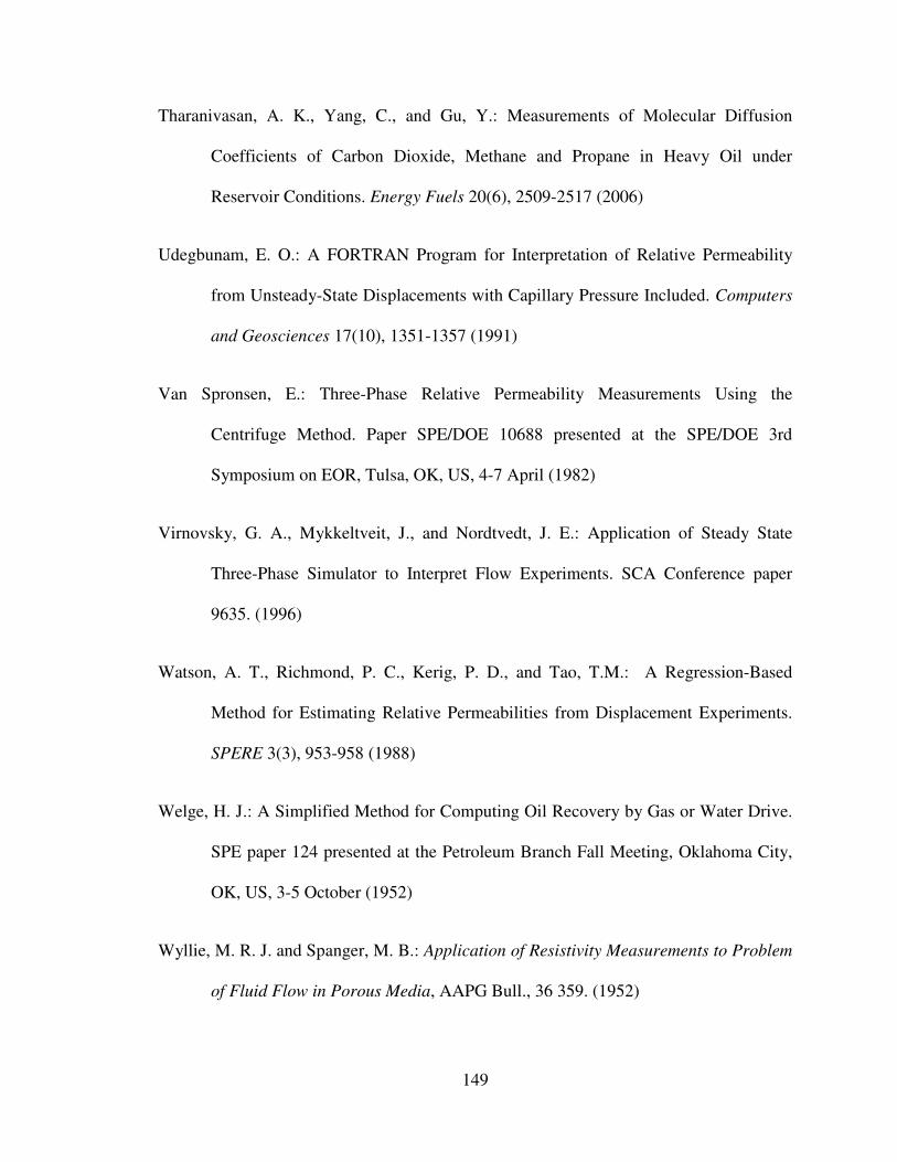
149
Tharanivasan, A. K., Yang, C., and Gu, Y.: Measurements of Molecular Diffusion
Coefficients of Carbon Dioxide, Methane and Propane in Heavy Oil under
Reservoir Conditions. Energy Fuels 20(6), 2509-2517 (2006)
Udegbunam, E. O.: A FORTRAN Program for Interpretation of Relative Permeability
from Unsteady-State Displacements with Capillary Pressure Included. Computers
and Geosciences 17(10), 1351-1357 (1991)
Van Spronsen, E.: Three-Phase Relative Permeability Measurements Using the
Centrifuge Method. Paper SPE/DOE 10688 presented at the SPE/DOE 3rd
Symposium on EOR, Tulsa, OK, US, 4-7 April (1982)
Virnovsky, G. A., Mykkeltveit, J., and Nordtvedt, J. E.: Application of Steady State
Three-Phase Simulator to Interpret Flow Experiments. SCA Conference paper
9635. (1996)
Watson, A. T., Richmond, P. C., Kerig, P. D., and Tao, T.M.: A Regression-Based
Method for Estimating Relative Permeabilities from Displacement Experiments.
SPERE 3(3), 953-958 (1988)
Welge, H. J.: A Simplified Method for Computing Oil Recovery by Gas or Water Drive.
SPE paper 124 presented at the Petroleum Branch Fall Meeting, Oklahoma City,
OK, US, 3-5 October (1952)
Wyllie, M. R. J. and Spanger, M. B.: Application of Resistivity Measurements to Problem
of Fluid Flow in Porous Media, AAPG Bull., 36 359. (1952)
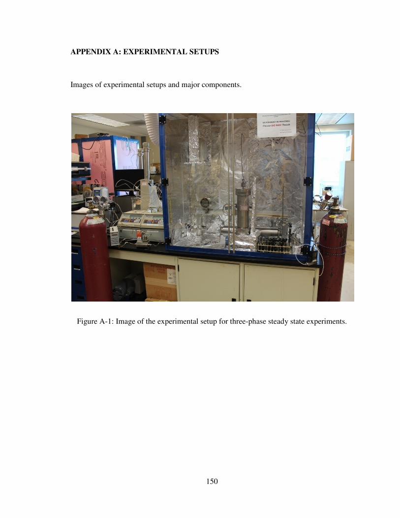
150
APPENDIX A: EXPERIMENTAL SETUPS
Images of experimental setups and major components.
Figure A-1: Image of the experimental setup for three-phase steady state experiments.
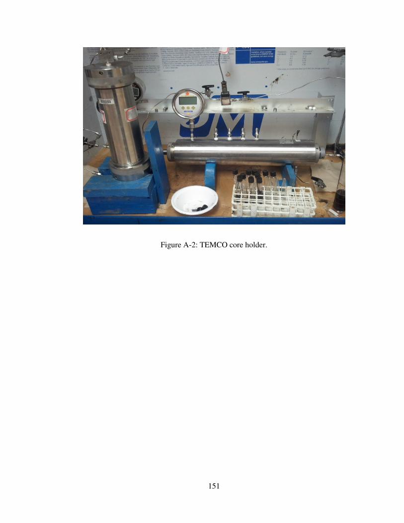
151
Figure A-2: TEMCO core holder.
152
Figure A-3: ISCO 500D (D Series) syringe pump.

153
Figure A-4: MAKITA heating gun (Model HG1100).

154
Figure A-5: Precise HIGH-TECH BRONKHORST gas flow controller.

155
Figure A-6: Resin-sealed separator used for separating liquid effluent from the produced
gas.

156
Figure A-7: COLE PARMER gas flow meter.

157
APPENDIX B: RESULTS OF THREE-PHASE DISPLACEMENT TESTS
Results from three-phase displacement experiments are presented below (see Section 5.4).
Conditions for all tests are summarized in Table (5.2).
Figure B.1: Results from three-phase displacement experiment#2.
0
10
20
30
40
50
60
0
0.02
0.04
0.06
0.08
0.1
0.12
0.14
0.16
0 200 400 600 800 1000 1200 1400
Pre
ssu
re D
rop
(p
si)
Pro
du
ctio
n (
PV
)
Time(min)
Oil Production
Water Production
Pressure Drop

158
Figure B.2: Results from three-phase displacement experiment#3
0
10
20
30
40
0
0.03
0.06
0.09
0.12
0.15
0.18
0.21
0 200 400 600 800 1000 1200
Pre
ssu
re D
rop
(p
si)
Pro
du
ctio
n (
PV
)
Time(min)
Oil Production
Water Production
Pressure Drop
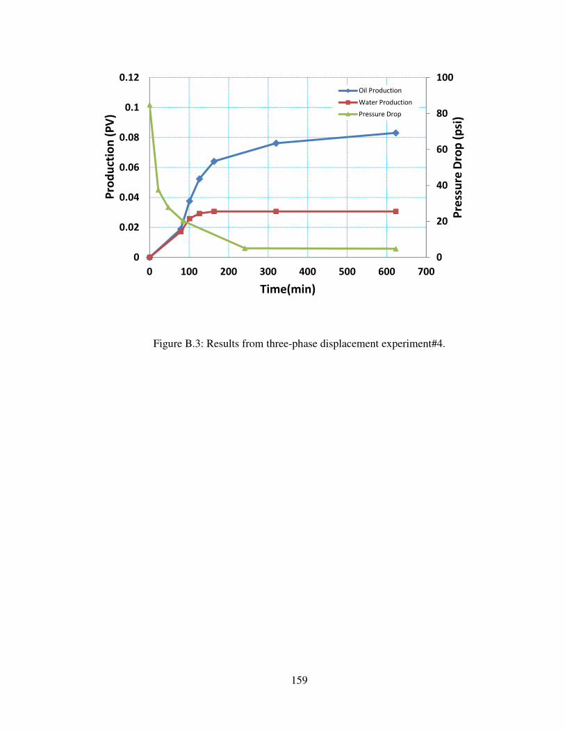
159
Figure B.3: Results from three-phase displacement experiment#4.
0
20
40
60
80
100
0
0.02
0.04
0.06
0.08
0.1
0.12
0 100 200 300 400 500 600 700
Pre
ssu
re D
rop
(p
si)
Pro
du
ctio
n (
PV
)
Time(min)
Oil Production
Water Production
Pressure Drop

160
Figure B.4: Results from three-phase displacement experiment#5.
0
10
20
30
40
50
60
70
0
0.02
0.04
0.06
0.08
0.1
0.12
0 200 400 600 800 1000 1200
Pre
ssu
re D
rop
(p
si)
Pro
du
ctio
n (
PV
)
Time(min)
Oil Production
Water Production
Pressure Drop

161
Figure B.5: Results from three-phase displacement experiment#6.
0
10
20
30
40
50
60
70
80
0
0.02
0.04
0.06
0.08
0.1
0.12
0.14
0.16
0 200 400 600 800 1000 1200
Pre
ssu
re D
rop
(p
si)
Pro
du
ctio
n (
PV
)
Time(min)
Oil Production
Water Production
Pressure Drop

162
Figure B.6: Results from three-phase displacement experiment#7.
0
10
20
30
40
50
60
70
80
0
0.02
0.04
0.06
0.08
0.1
0.12
0.14
0.16
0.18
0.2
0 200 400 600 800
Pre
ssu
re D
rop
(p
si)
Pro
du
ctio
n (
PV
)
Time(min)
Oil Production
Water Production
Pressure Drop

163
Figure B.7: Results from three-phase displacement experiment#8.
0
50
100
150
200
250
300
0
0.02
0.04
0.06
0.08
0 100 200 300 400
Pre
ssu
re D
rop
(p
si)
Pro
du
ctio
n (
PV
)
Time(min)
Oil Production
Water Production
Pressure Drop

164
APPENDIX C: MATHEMATICAL MODEL OF DEVELOPED SIMULATOR
Procedure presented here was derived from Basic Applied Reservoir Simulation
by Ertekin et al. (Ertekin et al., 2001). The simulation of hydrocarbon reservoir
experiments involves the simultaneous flow of oil, water, and gas transporting multiphase
fluid components. For a black oil three-phase displacement experiment described in the
chapter 5, the three fluid components present are heavy oil, water, and gas. Ignoring mass
transfer between phases, each fluid component is contained within its own phase, Figure
(C.1). A combination of Darcy’s law for multiphase flow with mass-conservation
equations provides the following equations that govern three-phase flow of heavy oil,
water, and gas in a one dimensional (x direction) horizontal core (Ertekin et al., 2001).

165
Figure C.1: Distribution of components among phases for a black oil system (Ertekin et
al., 2001)
Gas
Heavy Oil
Water
Gas
Water
Heavy Oil

166
For oil phase:
iiJ �@j�k �!�
��l� (iiJ)" mn = opq%
ii^ rs �l� t − =��j (C.1)
Water phase:
iiJ �@j�k �!�
��l� (iiJ)" mn = opq%
ii^ rs �l� t − =��j (C.2)
And gas phase:
iiJ M@j�k �!�
��l� (iiJ)P mn = opq%
ii^ Ns �l� O − =��j (C.3)
/� + /� + /� = 1 (C.4)
The terms qosc, qwsc, and qgsc refer to production (injection) rates of the oil, water,
and gas at standard condition. Subscripts o, w, and g refer to heavy oil, water, and gas.
Assumptions for above equations are as follows:
• One dimensional flow in x-direction
• Horizontal flow
• Negligible capillary forces
• Absolutely dead oil (solution gas ratio is zero)
• Homogonous and isotropic condition for rock properties (porosity and absolute
permeability)
• Isothermal condition
• No mass transfer between phases
Variables in Equations (5.1) to (5.4) are presented in Table (5.1) in field and
metric units.

167
The flow equations can be reduced to three equations with three unknowns of P,
Sw, and Sg if unknown So in the Equation (C.1) is replaced with 1-Sw-Sg from Equation
(C.4). So the flow equations set of black oil model in this formulation become:
iiJ �@j�k �!�
��l� (iiJ)" mn = opq%
ii^ rs(�� �� �)l� t − =��j (C.5)
iiJ �@j�k �!�
��l� (iiJ)" mn = opq%
ii^ rs �l� t − =��j (C.6)
iiJ M@j�k �!�
��l� (iiJ)P mn = opq%
ii^ Ns �l� O − =��j (C.7)
The analytical solution of these strongly non-linear partial difference equations is
too complex. The finite difference approach, as a numerical solution, is used to solve the
equation for P, Sw, Sg, and So. In this technique, the flow equations are discretized by use
of algebraic approximations of the second order derivatives with respect to space and the
first order derivatives with respect to time. Obtained equations are then solved by explicit
or implicit solutions.
The finite difference approximation of the second order partial derivatives are:
iiJ �@j�k �!�
��l� (iiJ)" mn ≈ m(v�m-) (C.8)

168
Table C.1: Variables used in flow equations (Ertekin et al., 2001).
Quantity Symbol Customary Unit Metric Unit Conversion Factor
Length x ft m 0.3048
Area A ft2 m
2 0.0929
Permeability k darcy µm2 0.9869
Viscosity µ cP Pa.s 0.001
Gas FVF*
Bg bbl/scf m3/std m
3 5.5519
Liquid FVF Bo, Bw bbl/STB m3/std m
3 1
Pressure P psia kPa 6.8947
Gas flow rate qgsc scf/D std m3/D 0.0286
Liquid flow
rate qosc, qwsc STB/D std m
3/D 0.1589
Absolute
temperature T ºR K 0.5555
Relative
permeability kr fraction fraction 1
Porosity φ fraction fraction 1
Saturation S fraction fraction 1
Compressibility
factor Z dimensionless dimensionless 1
Time t day day 1
Transmissibility
conversion
factor @j 1.127 86.4 × 10�� ---
Volume
conversion
factor zj 5.614583 1 ---
* FVF or Formation Volume Factor

169
iiJ �@j�k �!�
��l� (iiJ)" mn ≈ m(v�m-) (C.9)
iiJ M@j�k �!�
��l� (iiJ)P mn ≈ m(v�m-) (C.10)
Where transmissibilities are defined as:
v� = @j �h{J �!���l� (C.11)
v� = @j �h{J �!���l� (C.12)
v� = @j �h{J �!���l� (C.13)
Equations (C.5) to (C.7) now can be written in compact forms:
m|v�m-} = opq%
ii^ �s(�� �� �)l� " − =��j (C.14)
m|v�m-} = opq%
ii^ �s �l� " − =��j (C.15)
mUv�m-W = opq%
ii^ Ms �l� P − =��j (C.16)
Discretization in space means applying a finite difference approximation to the
second order derivative terms. In Figure (C.2), the core is divided into three gridblocks
with lengthmn\. The distance between grid point (i) and (i-1) ismn\��/#, and ismn\T�/#
between (i) and (i+1). The following relationship hold for both block centered and point
distributed girds.
mn\ = n\ − n\��/# (C.17)
mn\��/# = n\ − n\�� (C.18)

170
Figure C.2: Discretization in space.

171
mn\T�/# = n\T� − n\ (C.19)
The first derivative of an arbitrary variable f by the central difference
approximation with f evaluated at gridblock boundaries (i+1/2) and (i-1/2) in x direction
is:
i<iJ ≈ <A�*/&�<A�*/&
{JA (C.20)
Using Equation (C.20) twice for the left hand side of Equation (C.8) to (C.10)
gives:
m|v�m-} = v�\T�/#(-\T� − -\) − v�\�*&(-\ − -\��) (C.21)
m|v�m-} = v�\T�/#(-\T� − -\) − v�\�*&(-\ − -\��) (C.22)
mUv�m-W = v�\T�/#(-\T� − -\) − v�\�*&(-\ − -\��) (C.23)
For an arbitrary variable f, the partial derivative with respect to time becomes an
ordinary derivative at i if the space domain is fixed at grid point i.
(i<i^)\ = ��^ (2\) ≈ �
{^m^(2\) = �{^ (2\?T� − 2\?) (C.24)
where n+1 means one time step after time level n.
With this approach, the partial derivative term of the right hand side of Equations
(C.14) to (C.16) can be written as follows:
ii^ �s(�� �� �)l� " = �
{^ Mrs(�� �� �)l� t?T� − rs(�� �� �)l� t?P (C.25)
ii^ �s �l� " = �
{^ Mrs �l� t?T� − rs �l� t?P (C.26)
ii^ Ms �l� P = �
{^ �Ns �l� O?T� − Ns �l� O
?� (C.27)

172
Now implicit finite difference equations for all phases in the black oil model can
be written in the following compact form if the right hand sides of the equations are also
written at time level n+1:
v�\T*&?T�F-\T�?T� − -\?T�G − v�\�*
&?T�F-\?T� − -\��?T�G = op
q%{^ Mrs(�� �� �)
l� t?T� −rs(�� �� �)l� t?P − =��j?T� (C.28)
v�\T*&?T�F-\T�?T� − -\?T�G − v�\�*
&?T�F-\?T� − -\��?T�G = op
q%{^ Mrs �l� t?T� −rs �l� t?" − =��j?T� (C.29)
v�\T*&?T�F-\T�?T� − -\?T�G − v�\�*
&?T�F-\?T� − -\��?T�G = op
q%{^ �Ns �l� O
?T� −Ns �l� O
?P − =��j?T� (C.30)
To preserve mass conservation, the time difference operator acting on a function
should be expressed in terms of the difference of the unknowns. For an arbitrary variable,
such as f, an expansion scheme is described as conservative if the following identity is
satisfied:
m^2 = 2?T� − 2? (C.31)
The general conservative expansion formula is:
m^(���) = (��)?m^� + �?T�(�)?m^� + (��)?T�m^� (C.32)
For conservation expansion of a term m^((�/�)/��), assume that� = �,
� = 1/��, and � = /�. To preserve the conservative property of the expansion given by
m^(�) , m^(/\) , and m^(1/�\), it should be expressed as product of the chord slope
between successive time levels (n and n+1) and the time difference of the unknowns.
That is,
m^(�) = ��m^- (C.33)

173
m^(1/��) = (1/��)�m^- (C.34)
m^(/�) = m^/� (C.35)
Where
�� = sB�*�sBB�*��B (C.36)
(1/��)� = (�/l�)B�*�(�/l�)BB�*��B (C.37)
Substituting in Equation (C.32) gives:
m^(s �l� )=( �l�)?�′m^- + �?T�/�?( �l�)′m^- + ( s
l�)?T�m^/� (C.38)
Applying this approach for oil and gas phases gives the final form of the finite
difference equation for the black oil system.
v�\T*&?T�F-\T�?T� − -\?T�G − v�\�*
&?T�F-\?T� − -\��?T�G = ���F/�\?T� − /�\?G +
���F/�\?T� − /�\?G −=��j?T� (C.39)
v�\T*&?T�F-\T�?T� − -\?T�G − v�\�*
&?T�F-\?T� − -\��?T�G = ���F/�\?T� − /�\?G −
=��j?T� (C.40)
v�\T*&?T�F-\T�?T� − -\?T�G − v�\�*
&?T�F-\?T� − -\��?T�G = ���F-\?T� − -\?G +
���F/�\?T� − /�\?G − =��j?T� (C.41)
Where
��� = − opq%{^ (sl�)?T� (C.42)
��� = − opq%{^ (sl�)?T� (C.43)
��� = − opq%{^ ( s
l�)?T� (C.44)
��� = opq%{^�?T�( �
l�)�/�? (C.45)
��� = opq%{^ ( sl�)?T� (C.46)

174
In Equations (C.39) to (C.41), transmissibility terms of oil, water, and gas phases
for a homogenous core are in the form of:
v\±�/# = @j �h{J (�!µl)\±�/# (C.47)
Where the plus and minus signs in the subscripts are used to identify gridblock
boundaries in the positive and negative directions of the Cartesian coordinates. Single
point upstream weighting has been used to determine (�!µl)\T�/# at interblocks. It means
that at the boundary i+1/2 between gridblocks i and i+1
(�!;l)\T�/# = (�!;l)\ (C.48)
If flow is from gridblock i to gridblock i+1, and
(�!;l)\T�/# = (�!;l)\T� (C.49)
If flow is from gridblock i+1 to gridblock i.
In the three-phase displacement experiment described in the previous chapter, is
injected at a constant flow rate from one end of the core and the three-phase production
of oil, water, and gas occur at a constant pressure imposed by the back pressure regulator.
In Figure (C.2), it is assumed that gas is injected at grid i-1. For treatment of gas injection
at this grid, since flow always occur from gridblock i-1 to gridblock i, a no-flow
boundary is used at the left hand side of the gird i-1 by setting the left hand side
transmissibility equal to zero at all time steps. In the case of production under constant
pressure from the last grid i+1, an imaginary grid is assumed at the right hand side of the
grid i+1, with pressure equal to pressure set on the back pressure regulator for all time
steps.

175
In Equations (C.39) to (C.41), P, Sw, and Sg are the primary variables, and
unknowns to be solved for. All the coefficients in the equations, transmissibilities, as well
as storage coefficients, are functions of these unknowns. Thus, these equations cannot be
solved before the coefficients are calculated, and the coefficients cannot be calculated
before the unknown pressures and saturations have been solved. Obviously, a solution
method is needed that either iterates on the solution and updates coefficients and capillary
pressures until convergence is reached. A fully implicit technique has been used to solve
multiphase difference equations. Although this technique is an iterative method, there is
no concern about the stability of the solution at higher time levels. As the name implies,
all the equations for multiphase flow are solved simultaneously. The flowchart of the
implicit technique is presented in Figure (C.3). This scheme has been implemented in a
MATLAB software environment to simulate three-phase displacement experiments.
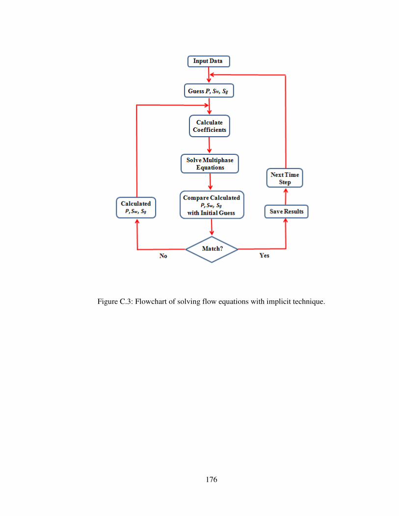
176
Figure C.3: Flowchart of solving flow equations with implicit technique.
177
APPENDIX D: MATLAB CODE FOR DEVELOPED SIMULATOR
Following program has been developed in the MATLAB software environment to
simulate three-phase displacement experiments. It couples with EXCEL software to
compare simulation results to observed data from experiments. Transmissibility functions
are presented after the main program. All input data to the simulator such as rock/fluid
properties are those presented in details in chapter 3. Initial condition (e.g. initial
saturation), injection rate, pressure constraint etc were also presented in chapter 5.
Calculations were performed with one minute as time step over ten grids in the x
direction. Time

178
clear all close all clc Length=input('Enter Length of the Core = '); Area=input('Enter Cross Sectional Area of The Core = '); Alpha=input('Enter Volume conversion factor = '); Beta=input('Enter Transmissibility conversion factor = '); Grids=input('Enter Number of Grids = '); Phi=input('Enter Porosity = '); Temp=input('Enter Temperature = '); K=input('Enter Absolute Permeability = '); Bw=input('Enter Formation Volume Factor for Water = '); Bo=input('Enter Formation Volume Factor for Oil = '); Visc_w=input('Enter Water Viscosity = '); Visc_o=input('Enter Oil Viscosity = '); x=1:Grids; Delta_x=Length/Grids; Phi=Phi.*ones(1,length(x)); K=K.*ones(1,length(x)); Bw=Bw.*ones(1,length(x)); Bo=Bo.*ones(1,length(x)); Visc_w=Visc_w.*ones(1,length(x)); Visc_o=Visc_o.*ones(1,length(x)); Vb=Area*Delta_x; Swi=input('Enter Irreducible Water Saturation = '); Sor=input('Enter Residual Oil Saturation = '); Delta_t=input('Enter Time Step = '); Delta_t=5*Delta_t; Time=input('Enter Final Time = '); t=0:Delta_t:Time; P_Initial=input('Enter Initial Core Pressure = '); Back_Pressure=input('Enter Pressure Set at BAck Pressure Regulator = '); Sw_Initial=input('Enter Initial Water Saturation = '); So_Initial=input('Enter Initial Oil Saturation = '); Q_Gas=input('Enter CO2 Injection Rate = '); Q_Gas=Q_Gas*0.00138; steps=length(t); P=ones(length(x),steps); So=ones(length(x),steps); Sw=ones(length(x),steps); Sg=ones(length(x),steps); P(:,1)=P_Initial; So(:,1)=So_Initial; Sw(:,1)=Sw_Initial; Sg(:,1)=Sg_Initial; Bg=ones(length(x),steps); Z_g=ones(length(x),steps); a=1; aa=a.*(Grids:-1:1); P(:,2)=P(:,1)+aa'; Error=1; for m=1:(steps-1) m=m; for i=1:length(x) if Sw(i,m)<=Swi Sw(i,m)=Swi; end

179
if Sg(i,m)<=0.01 Sg(i,m)=0.01; end end for i=1:length(x) if Sw(i,m)>=(1-Sor-0.01) Sw(i,m)=1-Sor-0.01; end if Sg(i,m)>=(1-Sor-Swi) Sg(i,m)=1-Sor-Swi; end end Sw(:,m+1)=Sw(:,m); Sg(:,m+1)=Sg(:,m); So(:,m+1)=1-Sw(:,m+1)-Sg(:,m+1); kk=1 Error=1; while Error>0.01 Visc_g=%Recall CO2 Viscosity at P and T% Z_g(:,m)=%Recall CO2 Compressibility Factor at P and T% Bg(:,m)=0.005035.*((Temp.*Z_g(:,m))./(P(:,m))); Z_g(:,m+1)=Z_g_Cal(P(:,m+1)); Bg(:,m+1)=0.005035.*((Temp.*Z_g(:,m+1))./(P(:,m+1))); Kro=%Recall Relative Permeability to Oil% Krw=%Recall Relative Permeability to Water% Krg=%Recall Relative Permeability to CO2% To=ones(length(x),2); for i=1:length(x) for o=1:2
To(i,o)=To_Cal(i,o,Beta,K,Area,Delta_x,Visc_o,Bo,Kro,P(:,m+1)); end end Tw=ones(length(x),2); for i=1:length(x) for o=1:2
Tw(i,o)=Tw_Cal(i,o,Beta,K,Area,Delta_x,Visc_w,Bw,Krw,P(:,m+1)); end end Tg=ones(length(x),2); for i=1:length(x) for o=1:2
Tg(i,o)=Tg_Cal(i,o,Beta,K,Area,Delta_x,Visc_g,Bg(:,m+1),Krg,P(:,m+1)); end end Oil_P=zeros(length(x)); Oil_Sw=zeros(length(x)); Oil_Sg=zeros(length(x)); Water_P=zeros(length(x)); Water_Sw=zeros(length(x)); Water_Sg=zeros(length(x)); Gas_P=zeros(length(x)); Gas_Sw=zeros(length(x)); Gas_Sg=zeros(length(x)); Cow=ones(length(x),1);

180
Cog=ones(length(x),1); Cww=ones(length(x),1); Cgg=ones(length(x),1); Cgp=ones(length(x),1); for i=1:length(x) Cow(i)=-(Vb/(Delta_t*Alpha))*(Phi(i)/Bo(i)); Cog(i)=-(Vb/(Delta_t*Alpha))*(Phi(i)/Bo(i)); Cww(i)=(Vb/(Delta_t*Alpha))*(Phi(i)/Bw(i)); Cgg(i)=(Vb/(Delta_t*Alpha))*(Phi(i)/Bg(i,m+1)); if P(i,m+1)==P(i,m) Cgp(i)=0; else A=((1/Bg(i,m+1))-(1/Bg(i,m)))/(P(i,m+1)-P(i,m)); Cgp(i)=(Vb/(Delta_t*Alpha))*Phi(i)*A*Sg(i,m); end end for i=1:length(x) if i==length(x) Oil_P(i,i)=-
(To(i,1)+2*(Beta*((K(i)*Area)/Delta_x)*(1/(Visc_o(i)*Bo(i)))*Kro(i))); Water_P(i,i)=-
(Tw(i,1)+2*(Beta*((K(i)*Area)/Delta_x)*(1/(Visc_w(i)*Bw(i)))*Krw(i))); Gas_P(i,i)=-
(Tg(i,1)+Cgp(i)+2*(Beta*((K(i)*Area)/Delta_x)*(1/(Visc_g(i)*Bg(i,m+1)))*
Krg(i))); else Oil_P(i,i)=-(To(i,1)+To(i,2)); Water_P(i,i)=-(Tw(i,1)+Tw(i,2)); Gas_P(i,i)=-(Tg(i,1)+Tg(i,2)+Cgp(i)); end end for i=1:length(x) Oil_Sw(i,i)=-Cow(i); Oil_Sg(i,i)=-Cog(i); Water_Sw(i,i)=-Cww(i); Water_Sg(i,i)=0; Gas_Sw(i,i)=0; Gas_Sg(i,i)=-Cgg(i); end for i=2:length(x) Oil_P(i-1,i)=To(i-1,2); Water_P(i-1,i)=Tw(i-1,2); Gas_P(i-1,i)=Tg(i-1,2); end for i=2:length(x) Oil_P(i,i-1)=To(i,1); Water_P(i,i-1)=Tw(i,1); Gas_P(i,i-1)=To(i,1); end Known_Oil=ones(length(x),1); Known_Water=ones(length(x),1); Known_Gas=ones(length(x),1); for i=1:length(x) if i==1 Known_Oil(i)=-Cow(i)*Sw(i,m)-Cog(i)*Sg(i,m); Known_Water(i)=-Cww(i)*Sw(i,m); Known_Gas(i)=-Cgp(i)*P(i,m)-Cgg(i)*Sg(i,m)-Q_Gas;
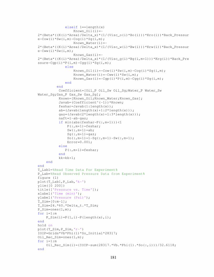
181
elseif 1==length(x) Known_Oil(i)=-
2*(Beta*((K(i)*Area)/Delta_x)*(1/(Visc_o(i)*Bo(i)))*Kro(i))*Back_Pressur
e-Cow(i)*Sw(i,m)-Cog(i)*Sg(i,m); Known_Water(i)=-
2*(Beta*((K(i)*Area)/Delta_x)*(1/(Visc_w(i)*Bw(i)))*Krw(i))*Back_Pressur
e-Cww(i)*Sw(i,m); Known_Gas(i)=-
2*(Beta*((K(i)*Area)/Delta_x)*(1/(Visc_g(i)*Bg(i,m+1)))*Krg(i))*Back_Pre
ssure-Cgp(i)*P(i,m)-Cgg(i)*Sg(i,m); else Known_Oil(i)=-Cow(i)*Sw(i,m)-Cog(i)*Sg(i,m); Known_Water(i)=-Cww(i)*Sw(i,m); Known_Gas(i)=-Cgp(i)*P(i,m)-Cgg(i)*Sg(i,m); end end Coefficient=[Oil_P Oil_Sw Oil_Sg;Water_P Water_Sw
Water_Sg;Gas_P Gas_Sw Gas_Sg]; Known=[Known_Oil;Known_Water;Known_Gas]; Javab=(Coefficient^(-1))*Known; feshar=Javab(1:length(x)); ab=(Javab(length(x)+1:2*length(x))); gaz=(Javab(2*length(x)+1:3*length(x))); naft=1-ab-gaz; if min(abs(feshar-P(:,m+1)))<1 P(:,m+1)=feshar; Sw(:,m+1)=ab; Sg(:,m+1)=gaz; So(:,m+1)=1-Sg(:,m+1)-Sw(:,m+1); Error=0.001; else P(:,m+1)=feshar; end kk=kk+1; end end T_Lab1=%Read Time Data For Experiment% P_Lab=%Read Observed Pressure Data from Experiment% figure (1) plot(T_Lab1,P_Lab,'k-') ylim([0 200]) title(['Pressure vs. Time']); xlabel('Time (min)'); ylabel('Pressure (Psi)'); T_Sim=[0:m-1]; T_Sim=24.*60.*Delta_t.*T_Sim; P_Sim=ones(1,m); for i=1:m P_Sim(i)=P(1,i)-P(length(x),i); end hold on plot(T_Sim,P_Sim,'r-') IOIP=Grids*Vb*Phi(1)*So_Initial*28317; Oil_Rec_Sim=ones(1,m); for i=1:m Oil_Rec_Sim(i)=(IOIP-sum(28317.*Vb.*Phi(1).*So(:,i)))/32.6118; end

182
T_Lab2=%Read Time Data For Experiment% Oil_Lab=%Read Observed Oil Production Data from Experiment% figure (2) plot(T_Lab2,Oil_Lab,'k-') ylim([0 0.5]) title(['Oil Recovery']); xlabel('Time (min)'); ylabel('Oil Recovery (Psi)'); hold on plot(T_Sim,Oil_Rec_Sim,'r-') IWIP=Grids*Vb*Phi(1)*Sw_Initial*28317; Water_Rec_Sim=ones(1,m); for i=1:m Water_Rec_Sim(i)=(IWIP-sum(28317.*Vb.*Phi(1).*Sw(:,i)))/32.6118; end Water_Lab=%Read Observed Water Production Data from Experiment% figure (3) plot(T_Lab2,Water_Lab,'k-') ylim([-0.05 0.22]) title(['Water Recovery']); xlabel('Time (min)'); ylabel('Water Recovery (Psi)'); hold on plot(T_Sim,Water_Rec_Sim,'r-') %Save Time Data from Simulation% %Save Pressure Data from Simulation% %Save Oil Production Data from Simulation% %Save Water Production Data from Simulation% close all clear all clc Swi=input('Enter Irreducible Water Saturation = '); Sor=input('Enter Residual Oil Saturation = '); x=0:0.1:100/(3^(0.5)); y=(3^(0.5)).*x; plot(x,y,'k-') clear x clear y hold on x=100/(3^(0.5)):0.1:200/(3^(0.5)); y=-(3^(0.5)).*(x-(200/(3^(0.5)))); plot(x,y,'k-') clear x clear y x=0:0.1:200/(3^(0.5)); for i=1:length(x) y(i)=0; end plot(x,y,'k-') clear x clear y hold on for i=10:10:90 x(i/10,:)=(1/(3^(0.5)))*i:0.1:-(1/(3^(0.5)))*i+200/(3^(0.5)); for j=1:length(x(i/10,:)) y(i/10,j)=i; end

183
plot(x(i/10,:),y(i/10,:),'b-.') clear x clear y end for i=10:10:90 x(i/10,:)=(2/(3^(0.5)))*i:0.1:((3^(0.5))/6)*(200+2*i); for j=1:length(x(i/10,:)) y(i/10,j)=(3^(0.5))*(x(i/10,j)-(2/(3^(0.5)))*i); end plot(x(i/10,:),y(i/10,:),'b-.') clear x clear y end for i=10:10:90 x(i/10,:)=(1/(3^(0.5)))*i:0.1:(2/(3^(0.5)))*i; for j=1:length(x(i/10,:)) y(i/10,j)=-(3^(0.5))*(x(i/10,j)-(2/(3^(0.5)))*i); end plot(x(i/10,:),y(i/10,:),'b-.') clear x clear y end i=Swi; x=(2/(3^(0.5)))*i:0.1:((3^(0.5))/6)*(200+2*i); for j=1:length(x) y(j)=(3^(0.5))*(x(j)-(2/(3^(0.5)))*i); end P1=plot(x,y,'g-'); clear x clear y clear i i=100-Sor; x=(1/(3^(0.5)))*i:0.1:(2/(3^(0.5)))*i; for j=1:length(x) y(j)=-(3^(0.5))*(x(j)-(2/(3^(0.5)))*i); end P2=plot(x,y,'m-'); clear x clear y clear i Oil1=%Read Oil Saturation Data, Path 1% Water1=%Read Water Saturation Data, Path 1% Oil1=100.*Oil1; Water1=100.*Water1; Gas1=100-Oil1-Water1; y1=Gas1; x1=-(2.*Oil1+y1-200)./(3^(0.5)); Krg1=%Read Gas Relative Permeability Data Correspond to Path 1% plot(x1,y1,'K.') Oil2=%Read Oil Saturation Data, Path 2% Water2=%Read Oil Saturation Data, Path 2% Oil2=100.*Oil2; Water2=100.*Water2; Gas2=100-Oil2-Water2; y2=Gas2; x2=-(2.*Oil2+y2-200)./(3^(0.5)); Krg2=%Read Gas Relative Permeability Data Correspond to Path 2%

184
plot(x2,y2,'K.') Oil3=%Read Oil Saturation Data, Path 3% Water3=%Read Oil Saturation Data, Path 3% Oil3=100.*Oil3; Water3=100.*Water3; Gas3=100-Oil3-Water3; y3=Gas3; x3=-(2.*Oil3+y3-200)./(3^(0.5)); Krg3=%Read Gas Relative Permeability Data Correspond to Path 3% plot(x3,y3,'K.') min1=min(Krg1); min2=min(Krg2); min3=min(Krg3); max1=max(Krg1); max2=max(Krg2); max3=max(Krg3); Krg_min=max([min1 min2 min3]); Krg_max=min([max1 max2 max3]); Curves=Krg_min:(Krg_max-Krg_min)/7:Krg_max; U=ones(3,2,(length(Curves)-2)); for i=2:(length(Curves)-1) U(1,1,i-1)=interp1(Krg1,x1,Curves(i)); U(1,2,i-1)=((3^(0.5))/3).*(U(1,1,i-1)-(2/(3^(0.5)))*(Swi)); U(2,1,i-1)=interp1(Krg2,x2,Curves(i)); U(2,2,i-1)=((3^(0.5))/6).*(U(2,1,i-1)-(2/(3^(0.5)))*(Swi)); U(3,1,i-1)=interp1(Krg3,x3,Curves(i)); U(3,2,i-1)=((3^(0.5))/(3/2)).*(U(3,1,i-1)-(2/(3^(0.5)))*(Swi)); end P3=plot(U(:,1,1),U(:,2,1),'ro'); P4=plot(U(:,1,2),U(:,2,2),'r+'); P5=plot(U(:,1,3),U(:,2,3),'r*'); P6=plot(U(:,1,4),U(:,2,4),'rs'); P7=plot(U(:,1,5),U(:,2,5),'rh'); P8=plot(U(:,1,6),U(:,2,6),'rv'); legend([P1 P2 P3 P4 P5 P6 P7
P8],'Swi','Sor',num2str(Curves(2)),num2str(Curves(3)),num2str(Curves(4))
,num2str(Curves(5)),num2str(Curves(6)),num2str(Curves(7))) close all clear all clc Swi=input('Enter Irreducible Water Saturation = '); Sor=input('Enter Residual Oil Saturation = '); x=0:0.1:100/(3^(0.5)); y=(3^(0.5)).*x; plot(x,y,'k-') clear x clear y hold on x=100/(3^(0.5)):0.1:200/(3^(0.5)); y=-(3^(0.5)).*(x-(200/(3^(0.5)))); plot(x,y,'k-') clear x clear y x=0:0.1:200/(3^(0.5)); for i=1:length(x) y(i)=0; end

185
plot(x,y,'k-') clear x clear y hold on for i=10:10:90 x(i/10,:)=(1/(3^(0.5)))*i:0.1:-(1/(3^(0.5)))*i+200/(3^(0.5)); for j=1:length(x(i/10,:)) y(i/10,j)=i; end plot(x(i/10,:),y(i/10,:),'b-.') clear x clear y end for i=10:10:90 x(i/10,:)=(2/(3^(0.5)))*i:0.1:((3^(0.5))/6)*(200+2*i); for j=1:length(x(i/10,:)) y(i/10,j)=(3^(0.5))*(x(i/10,j)-(2/(3^(0.5)))*i); end plot(x(i/10,:),y(i/10,:),'b-.') clear x clear y end for i=10:10:90 x(i/10,:)=(1/(3^(0.5)))*i:0.1:(2/(3^(0.5)))*i; for j=1:length(x(i/10,:)) y(i/10,j)=-(3^(0.5))*(x(i/10,j)-(2/(3^(0.5)))*i); end plot(x(i/10,:),y(i/10,:),'b-.') clear x clear y end i=Swi; x=(2/(3^(0.5)))*i:0.1:((3^(0.5))/6)*(200+2*i); for j=1:length(x) y(j)=(3^(0.5))*(x(j)-(2/(3^(0.5)))*i); end P1=plot(x,y,'g-'); clear x clear y clear i
i=100-Sor; x=(1/(3^(0.5)))*i:0.1:(2/(3^(0.5)))*i; for j=1:length(x) y(j)=-(3^(0.5))*(x(j)-(2/(3^(0.5)))*i); end P2=plot(x,y,'m-'); clear x clear y clear i Oil1=%Read Oil Saturation Data, Path 1% Water1=%Read Water Saturation Data, Path 1% Oil1=100.*Oil1; Water1=100.*Water1; Gas1=100-Oil1-Water1; y1=Gas1; x1=-(2.*Oil1+y1-200)./(3^(0.5));

186
Kro1=%Read Oil Relative Permeability Data Correspond to Path 1% plot(x1,y1,'K.') Oil2=%Read Oil Saturation Data, Path 2% Water2=%Read Water Saturation Data, Path 2% Oil2=100.*Oil2; Water2=100.*Water2; Gas2=100-Oil2-Water2; y2=Gas2; x2=-(2.*Oil2+y2-200)./(3^(0.5)); Kro2=%Read Oil Relative Permeability Data Correspond to Path 2% plot(x2,y2,'K.') Oil3=%Read Oil Saturation Data, Path 3% Water3=%Read Water Saturation Data, Path 3% Oil3=100.*Oil3; Water3=100.*Water3; Gas3=100-Oil3-Water3; y3=Gas3; x3=-(2.*Oil3+y3-200)./(3^(0.5)); Kro3=%Read Oil Relative Permeability Data Correspond to Path 3% plot(x3,y3,'K.') min1=min(Kro1); min2=min(Kro2); min3=min(Kro3); max1=max(Kro1); max2=max(Kro2); max3=max(Kro3); Kro_min=max([min1 min2 min3]); Kro_max=min([max1 max2 max3]); Curves=Kro_min:(Kro_max-Kro_min)/7:Kro_max; U=ones(3,2,(length(Curves)-2)); for i=2:(length(Curves)-1) U(1,1,i-1)=interp1(Kro1,x1,Curves(i)); U(1,2,i-1)=((3^(0.5))/3).*(U(1,1,i-1)-(2/(3^(0.5)))*(Swi)); U(2,1,i-1)=interp1(Kro2,x2,Curves(i)); U(2,2,i-1)=((3^(0.5))/6).*(U(2,1,i-1)-(2/(3^(0.5)))*(Swi)); U(3,1,i-1)=interp1(Kro3,x3,Curves(i)); U(3,2,i-1)=((3^(0.5))/(3/2)).*(U(3,1,i-1)-(2/(3^(0.5)))*(Swi)); end P3=plot(U(:,1,1),U(:,2,1),'ro'); P4=plot(U(:,1,2),U(:,2,2),'r+'); P5=plot(U(:,1,3),U(:,2,3),'r*'); P6=plot(U(:,1,4),U(:,2,4),'rs'); P7=plot(U(:,1,5),U(:,2,5),'rh'); P8=plot(U(:,1,6),U(:,2,6),'rv'); legend([P1 P2 P3 P4 P5 P6 P7
P8],'Swi','Sor',num2str(Curves(2)),num2str(Curves(3)),num2str(Curves(4))
,num2str(Curves(5)),num2str(Curves(6)),num2str(Curves(7))) close all clear all clc Swi=input('Enter Irreducible Water Saturation = '); Sor=input('Enter Residual Oil Saturation = '); x=0:0.1:100/(3^(0.5)); y=(3^(0.5)).*x; plot(x,y,'k-') clear x clear y
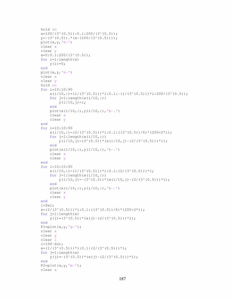
187
hold on x=100/(3^(0.5)):0.1:200/(3^(0.5)); y=-(3^(0.5)).*(x-(200/(3^(0.5)))); plot(x,y,'k-') clear x clear y x=0:0.1:200/(3^(0.5)); for i=1:length(x) y(i)=0; end plot(x,y,'k-') clear x clear y hold on for i=10:10:90 x(i/10,:)=(1/(3^(0.5)))*i:0.1:-(1/(3^(0.5)))*i+200/(3^(0.5)); for j=1:length(x(i/10,:)) y(i/10,j)=i; end plot(x(i/10,:),y(i/10,:),'b-.') clear x clear y end for i=10:10:90 x(i/10,:)=(2/(3^(0.5)))*i:0.1:((3^(0.5))/6)*(200+2*i); for j=1:length(x(i/10,:)) y(i/10,j)=(3^(0.5))*(x(i/10,j)-(2/(3^(0.5)))*i); end plot(x(i/10,:),y(i/10,:),'b-.') clear x clear y end for i=10:10:90 x(i/10,:)=(1/(3^(0.5)))*i:0.1:(2/(3^(0.5)))*i; for j=1:length(x(i/10,:)) y(i/10,j)=-(3^(0.5))*(x(i/10,j)-(2/(3^(0.5)))*i); end plot(x(i/10,:),y(i/10,:),'b-.') clear x clear y end i=Swi; x=(2/(3^(0.5)))*i:0.1:((3^(0.5))/6)*(200+2*i); for j=1:length(x) y(j)=(3^(0.5))*(x(j)-(2/(3^(0.5)))*i); end P1=plot(x,y,'g-'); clear x clear y clear i i=100-Sor; x=(1/(3^(0.5)))*i:0.1:(2/(3^(0.5)))*i; for j=1:length(x) y(j)=-(3^(0.5))*(x(j)-(2/(3^(0.5)))*i); end P2=plot(x,y,'m-'); clear x

188
clear y clear i Oil1=%Read Oil Saturation Data, Path 1% Water1=%Read Water Saturation Data, Path 1% Oil1=100.*Oil1; Water1=100.*Water1; Gas1=100-Oil1-Water1; y1=Gas1; x1=-(2.*Oil1+y1-200)./(3^(0.5)); Krw1=%Read Water Relative Permeability Data Correspond to Path 1% plot(x1,y1,'K.') Oil2=%Read Oil Saturation Data, Path 2% Water2=%Read Water Saturation Data, Path 2% Oil2=100.*Oil2; Water2=100.*Water2; Gas2=100-Oil2-Water2; y2=Gas2; x2=-(2.*Oil2+y2-200)./(3^(0.5)); Krw2=%Read Water Relative Permeability Data Correspond to Path 2% plot(x2,y2,'K.') Oil3=%Read Oil Saturation Data, Path 3% Water3=%Read Water Saturation Data, Path 3% Oil3=100.*Oil3; Water3=100.*Water3; Gas3=100-Oil3-Water3; y3=Gas3; x3=-(2.*Oil3+y3-200)./(3^(0.5)); Krw3=%Read Water Relative Permeability Data Correspond to Path 3% plot(x3,y3,'K.') min1=min(Krw1); min2=min(Krw2); min3=min(Krw3); max1=max(Krw1); max2=max(Krw2); max3=max(Krw3); Krw_min=max([min1 min2 min3]); Krw_max=min([max1 max2 max3]); Curves=Krw_min:(Krw_max-Krw_min)/7:Krw_max; U=ones(3,2,(length(Curves)-2)); for i=2:(length(Curves)-1) U(1,1,i-1)=interp1(Krw1,x1,Curves(i)); U(1,2,i-1)=((3^(0.5))/3).*(U(1,1,i-1)-(2/(3^(0.5)))*(Swi)); U(2,1,i-1)=interp1(Krw2,x2,Curves(i)); U(2,2,i-1)=((3^(0.5))/6).*(U(2,1,i-1)-(2/(3^(0.5)))*(Swi)); U(3,1,i-1)=interp1(Krw3,x3,Curves(i)); U(3,2,i-1)=((3^(0.5))/(3/2)).*(U(3,1,i-1)-(2/(3^(0.5)))*(Swi)); end P3=plot(U(:,1,1),U(:,2,1),'ro'); P4=plot(U(:,1,2),U(:,2,2),'r+'); P5=plot(U(:,1,3),U(:,2,3),'r*'); P6=plot(U(:,1,4),U(:,2,4),'rs'); P7=plot(U(:,1,5),U(:,2,5),'rh'); P8=plot(U(:,1,6),U(:,2,6),'rv'); legend([P1 P2 P3 P4 P5 P6 P7
P8],'Swi','Sor',num2str(Curves(2)),num2str(Curves(3)),num2str(Curves(4))
,num2str(Curves(5)),num2str(Curves(6)),num2str(Curves(7)))

189
function T = Tg_Cal(i,dir,Beta,K,Area,Delta_x,Visc_g,Bg,Krg,P); % Tg_Cal function calculate transmiscibility for each cell: % Detailed explanation goes here:
switch dir case 1 if i==1 T=0; else if P(i)>=P(i-1) T=Beta*((K(i)*Area)/Delta_x)*(1/(Visc_g(i)*Bg(i)))*Krg(i); else T=Beta*((K(i-1)*Area)/Delta_x)*(1/(Visc_g(i-1)*Bg(i-
1)))*Krg(i-1); end end case 2 if i==length(P) T=0; else if P(i)>=P(i+1) T=Beta*((K(i)*Area)/Delta_x)*(1/(Visc_g(i)*Bg(i)))*Krg(i); else
T=Beta*((K(i+1)*Area)/Delta_x)*(1/(Visc_g(i+1)*Bg(i+1)))*Krg(i+1); end end end
end

190
function T = To_Cal(i,dir,Beta,K,Area,Delta_x,Visc_o,Bo,Kro,P); % To_Cal function calculate transmiscibility for each cell: % Detailed explanation goes here:
switch dir case 1 if i==1 T=0; else if P(i)>=P(i-1) T=Beta*((K(i)*Area)/Delta_x)*(1/(Visc_o(i)*Bo(i)))*Kro(i); else T=Beta*((K(i-1)*Area)/Delta_x)*(1/(Visc_o(i-1)*Bo(i-
1)))*Kro(i-1); end end case 2 if i==length(P) T=0; else if P(i)>=P(i+1) T=Beta*((K(i)*Area)/Delta_x)*(1/(Visc_o(i)*Bo(i)))*Kro(i); else
T=Beta*((K(i+1)*Area)/Delta_x)*(1/(Visc_o(i+1)*Bo(i+1)))*Kro(i+1); end end end
end

191
function T = Tw_Cal(i,dir,Beta,K,Area,Delta_x,Visc_w,Bw,Krw,P); % Tw_Cal function calculate transmiscibility for each cell: % Detailed explanation goes here:
switch dir case 1 if i==1 T=0; else if P(i)>=P(i-1) T=Beta*((K(i)*Area)/Delta_x)*(1/(Visc_w(i)*Bw(i)))*Krw(i); else T=Beta*((K(i-1)*Area)/Delta_x)*(1/(Visc_w(i-1)*Bw(i-
1)))*Krw(i-1); end end case 2 if i==length(P) T=0; else if P(i)>=P(i+1) T=Beta*((K(i)*Area)/Delta_x)*(1/(Visc_w(i)*Bw(i)))*Krw(i); else
T=Beta*((K(i+1)*Area)/Delta_x)*(1/(Visc_w(i+1)*Bw(i+1)))*Krw(i+1); end end end
end

192
APPENDIX E: 3RELPERM PLOT
E.1 Applications
3RelPerm Plot, Figure (E.1) is an easy-to-use software specially designed to represent
three-phase relative permeability data in ternary diagrams. However, it can be used in
other engineering and science disciplines such as:
• Petroleum Engineering (PVT)
• Chemical Engineering / Physical Chemistry
• Geology / Mineralogy / Petrophysics / Petrology / Soil Science
• Metallurgy
• Other Physical Sciences
E.2 System Requirement
3RelPerm Plot is a portable, executable (.exe) file developed in Microsoft Visual Studio
2010. A .net Framework is required to run the application.

193
Figure E.1: 3RelPerm Plot Interface (original in color).

194
E.3 Features
E.3.1 Three-Phase Flow Zone
The Boundary settings allow the user to confine data in an arbitrary triangle inside the
main triangle. This ability is very useful to present three-phase relative permeability data
since the concept of three-phase flow zone is encountered. As an example, Figure E.2
shows how relative permeabilities to gas phase are plotted in a confined three-phase flow
zone. The bottom edge value (entered zero) represents zero irreducible gas saturation; the
right edge value (entered 40) represents 40% residual oil saturation; and the left edge
value (entered 3) represents 3% irreducible water saturation. Values at the vertices of the
confined triangle should be known (yellow circles). In the example shown in Figure E.2,
relative permeability at the top vertex (So = 40%, Sw = 3%, Sg = 57%) is entered as 0.33,
the right vertex (So = 40%, Sw = 60%, Sg = 0%) and the left vertex (So = 97%, Sw = 3%,
Sg = 0%) are entered as zero.

195
Figure E.2: Plotting a three-phase flow zone with 3RelPerm Plot (original in color).

196
E.3.2 User-Friendly Setting
3RelPerm Plot provides a variety of colours for colour mapping, gridlines, marker, and
boundary lines (Figure E.3). In addition, marker size and thickness of boundary lines can
be changed in the setting. Also user is able to add/remove colour mapping, gridlines, data
points, and boundary lines.

197
Figure E.3: Colour options in 3RelPerm Plot. (from www.rapidtables.com) (original in
color).
198
E.3.3 Interpolation
3RelPerm Plot exceptionally allows user to analyze and interpolate within the ternary
diagram. Once the mouse curser is hovered within the main triangle, all information
appears in the top left corner of the plotting panel (Figure E.4). As an example, following
information can be read based on the location of the curser within the ternary diagram:
Top Phase: 54%
Left Phase: 23%
Right Phase: 23%
Corresponding property: 0.508515136469834

199
Figure E.4: Interpolation between point in 3RelPerm Plot (original in color).

200
E.4 Meshing/Graphics Algorithm:
Delaunay Triangulation with incremental technique has been used to build meshes and
then color-mapping. The procedure is as following:
1. The first triangle constructed is called a supertriangle. It is an equilateral triangle that
entirely contains the convex hull of the points to be triangulated. The vertices of this
construction will be removed in the last step, leaving the triangulated network.
2. Points to be triangulated are added one by one. The list of points is ordered by their y
co-ordinate.
3. Circumcircles pass through the three vertices of each triangle in the network. As each
additional point is added to the structure, triangles who's circumcircle contains the new
point are identified and their associated triangles removed.
5. New triangles are formed between the most recently inserted point and the segments of
the void left after removing the triangles.
6. After the final point is added, the vertices of the supertriangle and any triangles that
share these vertices are removed.
Corresponding algorithm has been developed independently and successfully examined
several times with MATLAB software, Figure E.5.

201
Figure E.5: The Delaunay Triangulation of a random set of 300 points in a plane by
MATLAB algorithm (TOP) and self-developed algorithm (BOTTOM) (original in color).

202
APPENDIX F: FINAL MATCHING RESULTS
Results presented here are the final results of matching observed data from the
three-phase displacement experiments (pressure drop, oil production, and water
production) with those obtained from the developed numerical simulator. Corresponding
relative permeability isoperms have been presented in Chapter 6.

203
Figure F.1: Results from matching test#2 for saturation path # 1, top (pressure drop),
middle (oil production), and bottom (water production).
0
10
20
30
40
50
60
0 200 400 600 800 1000 1200
ΔP
(p
si)
Time(min)
Experiment
Simulation
0
0.02
0.04
0.06
0.08
0.1
0.12
0.14
0 200 400 600 800 1000 1200
Oil
Pro
d.
(PV
)
Time(min)
Simulation
Experiment
0
0.01
0.02
0.03
0.04
0.05
0 200 400 600 800 1000 1200
Wa
ter
Pro
d.
(PV
)
Time(min)
Simulation
Experiment

204
Figure F.2: Results from matching test#3 for saturation path # 1, top (pressure drop), middle (oil
production), and bottom (water production).
0
5
10
15
20
25
30
35
40
0 200 400 600 800 1000 1200
ΔP
(p
si)
Time(min)
Experiment
Simulation
0
0.04
0.08
0.12
0.16
0.2
0 200 400 600 800 1000 1200
Oil
Pro
d.
(PV
)
Time(min)
Simulation
Experiment
0
0.02
0.04
0.06
0.08
0 200 400 600 800 1000 1200
Wa
ter
Pro
d.
(PV
)
Time(min)
Simulation
Experiment

205
Figure F.3: Results from matching test#4 for saturation path # 1, top (pressure drop), middle (oil
production), and bottom (water production).
0
20
40
60
80
100
0 100 200 300 400 500 600 700
ΔP
(p
si)
Time(min)
Experiment
Simulation
0
0.02
0.04
0.06
0.08
0.1
0 100 200 300 400 500 600 700
Oil
Pro
d.
(PV
)
Time(min)
Simulation
Experiment
0
0.01
0.02
0.03
0.04
0 100 200 300 400 500 600 700
Wa
ter
Pro
d.
(PV
)
Time(min)
Simulation
Experiment

206
Figure F.4: Results from matching test#5 for saturation path # 1, top (pressure drop), middle (oil
production), and bottom (water production).
0
10
20
30
40
50
60
70
80
0 100 200 300 400 500 600 700 800 900 1000 1100 1200
ΔP
(p
si)
Time(min)
Experiment
Simulation
0
0.02
0.04
0.06
0.08
0.1
0.12
0 100 200 300 400 500 600 700 800 900 1000 1100 1200
Oil
Pro
du
ctio
n (
PV
)
Time(min)
Simulation
Experiment
0
0.01
0.02
0.03
0.04
0 100 200 300 400 500 600 700 800 900 1000 1100 1200
Wa
ter
Pro
du
ctio
n (
PV
)
Time(min)
Simulation
Experiment

207
Figure F.5: Results from matching test#5 for saturation path # 1, top (pressure drop), middle (oil
production), and bottom (water production).
0
10
20
30
40
50
60
70
80
0 100 200 300 400 500 600 700 800 900 1000 1100 1200
ΔP
(p
si)
Time(min)
Experiment
Simulation
0
0.02
0.04
0.06
0.08
0.1
0.12
0.14
0.16
0 100 200 300 400 500 600 700 800 900 1000 1100 1200
Oil
Pro
du
ctio
n (
PV
)
Time(min)
Simulation
Experiment
0
0.01
0.02
0.03
0.04
0.05
0.06
0 100 200 300 400 500 600 700 800 900 1000 1100 1200
Wa
ter
Pro
du
ctio
n (
PV
)
Time(min)
Simulation
Experiment

208
Figure F.6: Results from matching test#7 for saturation path # 1, top (pressure drop), middle (oil
production), and bottom (water production).
0
15
30
45
60
75
90
0 100 200 300 400 500 600 700 800
ΔP
(p
si)
Time(min)
Experiment
Simulation
0
0.03
0.06
0.09
0.12
0.15
0.18
0.21
0 100 200 300 400 500 600 700 800
Oil
Pro
du
ctio
n (
PV
)
Time(min)
Simulation
Experiment
0
0.01
0.02
0.03
0.04
0.05
0.06
0.07
0 100 200 300 400 500 600 700 800
Wa
ter
Pro
du
ctio
n (
PV
)
Time(min)
Simulation
Experiment

209
Figure F.7: Results from matching test#8 for saturation path # 1, top (pressure drop), middle (oil
production), and bottom (water production).
0
50
100
150
200
250
300
0 100 200 300 400
ΔP
(p
si)
Time(min)
Experiment
Simulation
0
0.02
0.04
0.06
0.08
0 100 200 300 400
Oil
Pro
du
ctio
n (
PV
)
Time(min)
Simulation
Experiment
0
0.01
0.02
0.03
0.04
0 100 200 300 400
Wa
ter
Pro
du
ctio
n (
PV
)
Time(min)
Simulation
Experiment