1

Experiment Nr.10 Superconductivity

(Physics Department E10)

I. Theory: Kamerlingh Onnes was the discoverer of the superconductivity. He investigated the conductivity of metals and its rest resistance (Matthiesensche rule) at low temperatures in 1911. At mercury he found an abruptly disappearance of the electrical resistance at the so called critical temperature Tc (fig. 1). This new state which show many metals, is referred to as superconductive phase. This appears when the temperature of the sample, a magnetic field affecting the sample and a transportation current through the sample are not to large. fig. 1.: Resistance of Hg. At the critical Temperature Tc=4.2 K is a jump of the resistance to 0 Ω. Properties of a superconductor in an external magnetic field We make the following thought experiment: The superconductor (SC) is cooled without an external magnetic field at a temperature below its critical temperature. An external field is then applied. The following laws are valid:

a) law of induction: EtB

×∇=∂∂

−

b) Ohm's law: jjEEj ρσ

σ ==⇒= σ : electrical conductivity

ρ: resistivitiy In the superconducting phase is R = 0 and with A

lR ρ= follows that

000 =∂∂⇒=⇒= tBEρ

This means .constBi = inside the superconductor.

2

It is the idea that due to the rise of the external field eddy currents (so called schielding currents) are started up in the superconductor (Lenz's rule). These don't fade away because of the superconductivity. The magnetic field produced by the permanent constant current protects the superconductor against the penetration of the external field. The question arises now how such an inner magnetic field Bi can be measured. This is clarified in fig. 2. fig. 2: schematic diagram of the magnetic field measurement inside the superconductor An inductance coil is wound round a long thin superconductive wire. After the SC has been cooled under its critical temperature, an external field Ba is applied to the superconductor and increased. If the inner field Bi in the SC changes, there is a flux change in the coil so that an induced voltage is measurable. This voltage is

∫∝⇒∝Φ=− dtUBBU indiiind With the help of an integrator a temporal integration of the signal is carried out. The measured value at the output of the integrator is proportional to Bi. As a result one receives the curve shown in figure 3. Fig. 3: dependence of the magnetic field inside the SC Bi from the external field Ba for a type-I SC. As long as the external field Ba is below a certain critical field Bc (critical Field strength), no induced voltage is measurable at the coil. No flux change takes place in the coil. This means that still Bi = 0 in the SC. If the critical value Bc is reached it comes to a collapse of the superconductivity. The superconductor changes into its normal conductive state and the eddy currents fade away. This leads to a flux change in the coil which is measured. Like in fig. 3, this process recognizably takes place at Bc abruptly. Above Bc inner and external field are equal. However the magnetic field doesn't drop off abruptly at the surface in the superconducting state from the value Ba to zero, but decreases within the London penetration depth λ to the 1/e part of the value. This is shown schematically in fig. 4. The magnetic field is shown versus the width x of the superconductor. At the edges x = 0 or x = d the magnetic field falls

3

exponentially against zero. Outside the sample the external field Ba is constant. The resulting penetration depth lies in the range of 10-6 – 10-8 m. fig. 4: Exponential decay of the magnetic field Bi inside the superconductor. Ba is constant outside. Often the magnetization M is shown versus the magnetic field, too. The definition is:

MBB ai μ+= respectively

If we look at equal directional sizes, then the vector notation can be renounced: Figure 5 shows the magnetization as a function of Ba for an ideal and real superconductor type I. This diagrams emphasizes the behaviour of the superconductor as an ideal diamagnet with the susceptibility χ = -1 (slope of the straight line). The magnetization drops off vertically for a ideal superconductor at Bc since the magnetic field penetrates into the sample. Fig. 5: Magnetization as a function of the external field for a type I superconductor. The superconductor behaves as an ideal diamagnet.

a) ideal superconductor b) real superconductor

In real samples there are complications. Firstly, the applied filed is deformed by the object itself. In the fall of a ball there is a field B > Ba (see fig. 6) at the equator. Fig. 6: Deformation of the field due to a spherical superconductor.

From this it follows that aBN

M−

=−1

10μ (N: Demagnetizing factor) , to ensure Bi=0, and

that the magnetic field already starts to penetrate at a field Ba of ceffc BNB )1( −= (cf. fig. 5 b).

ia BBM −=− 0μ

ia BBM −=− 0μ

4

During the penetration the field distortion is reduced so that the superconductivity disappears completely not until Ba=Bc. This means at a resistance measurement (task 2), Ba = Bc at the field at which R returns to the normal conductive value completely (fig. 7). Fig. 7: Bc determination by the resistance of the sample. The Meissner-Ochsenfeld-Effect This was found 1933 by W. Meissner and R. Ochsenfeld. Unlike the thought experiment from above a magnetic field is applied first and the sample then cooled down. The question how the sample will behave arises if the superconducting phase appears by exceeding the Bc (T) curve. The field inside should remain constant. One would expect a “frozen” field in the sample. But the field is pressed out from the sample instead. Again is Bi = 0. This means that the eddy currents mentioned above start to flow spontaneously. The superconductivity requires apparently that Bi =0 independent if it was cooled with or without field. The type-II superconductor Characteristically for a superconductor type-II is the behaviour in a magnetic field. Two critical fields appear here, on the one hand the so called lower critical field Bc1 (lower critical field) and on the other hand the upper critical field Bc2 (upper critical field). Figure 8 shows the curve of the field Bi inside the superconductor versus the external field Ba. As long as the external field is smaller than the critical field Bc1 we are, as in the case of the superconductor type-I, in the Meissner phase. This means that the field inside is zero. If the critical field Bc1 is exceeded, one gets the mixed state or the Shubnikov phase. Here is a coexistence from normal conductive areas and superconductive areas. The field penetrates in so called flux lines (vortecies) into the superconductor at Bc1. A flux line you can imagine as a normal conductive line through the sample, around which flows a ring current from Cooper pairs or a current curl (= vortex). Fig. 8: dependence of the magnetic field inside the SC Bi from the external field Ba for a type-II SC. A flux line encloses exactly one flux quantum φ0 which is defined as:

2110 1022 Tcme

h −×==φ

5

With an increasing external field Ba more and more flux lines penetrate into the superconductor. Therefore the flux rises inside the sample, as well as the macroscopically averaged field Bi which is given as: Here is: N = number of vortices inside the sample A = cross-sectional area of the sample If Bc2 is reached (at the intersection point of the curve with the bisector), only overlaped normal conductive flux lines are existent. The superconductivity break down now completely and again Bi=Ba (fig. 8) Instead of the inner field Bi one usually plots the magnetization versus the external field Ba. This is showed in figure 9 (compare fig. 5 to this: Magnetization of the SC type I). At first the magnetization rises linearly. The superconductor shows the normal diamagnetic behaviour. If Bc1 is reached, the curve drop down. The field penetrates now into the superconductor until the complete sample is finally normal conductive reaching Bc2 . fig. 9: Magnetization versus the external field for a superconductor type-II. Completing the dependence of the critical magnetic field Bc2 of the temperature is shown (fig. 10). In comparison with the superconductor type I, the superconductor type II withstands considerably higher field strengths. The temperature dependence is similar to the SC type I. fig. 10: Temperature dependence of the critical field for different SC type II. One receives a similar graph as in the case of the SC type I but obviously higher fields are reached.

(Kittel)

( ) 0 φANB i =

6

Heat capacity of a superconductor is defined as follows: The difference of the heat capacity between superconductor (SC) and normal conductor (NC) shall be specified now. It is: We want to illustrate this (fig. 11) graphically: Fig. 11: Graphically derived difference of the heat capacity between SC and NC. The entropy difference of a superconductor and a normal conductor are given in picture a). Qualitatively chart b) shows the derivation of the curve in a). The minimum of a) can be seen as zero-crossing in b). In b) the curve reaches a maximum at T=0 resp.T=Tc, because of the maximum slope at the same points in a). The difference of the heat capacity is given with multiplying b) by the temperature straight lines (pictures c)). Since the temperature straight line goes through the origin, ΔC=0 at T=0 follows from the multiplication. In addition, ΔC is for T>Tc zero. The heat capacity of the normal conductor is known from the solid state physics. At metals it is consisting of an electronic and phononic (lattice vibrations) part. For temperatures far below the Debye-temperature it is: CNC=γ T+A T ³ γT represents the electronic and AT³ the phononic part. Mostly γ is known as Sommerfeld-parameter.

dTdST

dTdQC ==

( )cT

ccNCSCNCSC dT

dBTSSdTdTCC

2

0⎟⎠⎞

⎜⎝⎛=−=−

μ

7

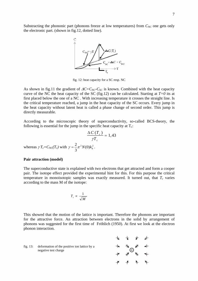
Substracting the phononic part (phonons freeze at low temperatures) from CNC one gets only the electronic part. (shown in fig.12, dotted line).

fig. 12: heat capacity for a SC resp. NC As shown in fig.11 the gradient of ΔC=CNC-CSC is known. Combined with the heat capacity curve of the NC the heat capacity of the SC (fig.12) can be calculated. Starting at T=0 its at first placed below the one of a NC . With increasing temperature it crosses the straight line. Is the critical temperature reached, a jump in the heat capacity of the SC occurs. Every jump in the heat capacity without latent heat is called a phase change of second order. This jump is directly measurable. According to the microscopic theory of superconductivity, so-called BCS-theory, the following is essential for the jump in the specific heat capacity at Tc:

whereas γ Tc=CNC(Tc) with 22 )0(32

bkNπγ = .

Pair attraction (model) The superconductive state is explained with two electrons that get attracted and form a cooper pair. The isotope effect provided the experimental hint for this. For this purpose the critical temperature in monoisotopic samples was exactly measured. It turned out, that Tc varies according to the mass M of the isotope: This showed that the motion of the lattice is important. Therefore the phonons are important for the attractive force. An attraction between electrons in the solid by arrangement of phonons was suggested for the first time of Fröhlich (1950). At first we look at the electron phonon interaction. fig. 13: deformation of the positive ion lattice by a

negative test charge

43,1)(=

Δ

c

c

TTC

γ

MTc

1∝

8

We put a negative test charge (electron) into the lattice of positive ion-cores (fig.13) Due to the coulomb-attraction the lattice is polarized. The charge strength of the point charge shall oscillate with (i.e. the electron moves through the place x => “oscillation of charge” at the place x) For this reason the attractive force also oscillates so that we receive a forced oscillation of the lattice. We simplest can treat this problem with the Einstein model (all atoms have the same resonant frequency ωE). The resulting amplitude and phase (between vibrating atom and charge oscillation) of the movement is shown in fig. 14. Fig. 14: amplitude and phase of the displacement due to

the oscillating charge strength If the frequency of the atoms is ω<<ωE, the lattice swings in-phase with the oscillating charge. I.e. the negative charges get bigger, the displacement then gets greater, too, so that more positive charges are available in the area of the negative charges. The positive charges only partly protect the negative one because of the stiffness of the lattice. Is ω ωE , the amplitude of the positive charges grows into resonance and the amplitude of the negative oscillating charges predominates. Then one speaks of “over screening” the negative charges by the positive ones. The phase shift is not pronounced strongly yet. In this case a second negative charge can be attracted by this “over screening”, what effectively corresponds to a positive interaction of two negative charges. So a Cooper pair arises from the exchange of phonons. If ω>ωE, the lattice oscillates in opposition (phase shift around π). If the negative charges are small, there are more positive charges and reversed. The negative potential gets amplified and no longer screened with that. The energy gap: Below Tc more and more Cooper pairs arise with decreasing temperature until all electrons are paired at T=0. On the other hand this means that for T>0 there are still normal conductive electrons. They are also named as quasiparticles. Through this coupling the electrons are able to decrease their energy. The energy difference between normal conductive electrons and superconductive electrons is called energy gap. The dependence of this energy gap Δ on the temperature is ploted in fig. 15. Near the critical temperature it decreases rapidly down to zero. Quantitatively follows from the BCS-theory:

tieqqq ω10 +=

<~

cBTk52,32 0 =Δ

9

fig. 15: dependence of the energy gap on the temperature

The new superconductors In the years 1986/87 a new class of superconductors was developed, based on metaloxids and having a structure similar to perovskite (fig.16). The compound YBa2Cu3O7-x (x≈0,2) has a Tc of about 90K, that is above the boiling temperature of liquid N2. The essential mechanism for superconductivity in these materials, is not yet understood completely. Superconductivity takes place in the CuO2 – planes. fig. 16: High-Temperature-Superconductor YBa2Cu3O7-x

II. Experiments Cryostat The samples for task 1 to 4 are placed in a “bath-cryostat” (fig.17). The cryostat consists of two double walled and mirrored-glass vessels (=Dewar). The gaps are evacuated for the reduction of thermal conduction. Besides the reflecting glass the thermal radiation is primarily reduced by pre-cooling with liquid N2 (why?). Via a pump-system is the helium part of the cryostat connected with the return-line to the helium-condenser. For cooling down N2 is filled first. After about one hour liquid helium can be filled into the cryostat. For this purpose a U-shaped siphon is used. This may only be done under supervision of the assistant. Caution: The pressure in the cryostat may not increase about normal pressure at any time during the rest of the experiment. Always open valve V3 on time. (Danger of Explosion). The liquid helium level can be checked by view slits (lamp). A ventilator prevents fogging.

10

fig. 17: experimental set-up Measuring program The data of all experiments are recorded with a computer which is equipped with a A/D converter card. The user name is “Praktikum” and the password is the uncapitalised short form of a well known high temperature superconductor (password?). After launching the LabView program „Praktikum“ you are in the main menu of the practical course-software; from here you can start every individual measuring program for every single part of the experiment. The basic construction of every measuring program is the same. On a big diagram area the current measurement is shown as a white point, the measured values are colored. Using the buttons “Messwert” or “Messung” you can take single measurements or start a continuing measurement, depending on the part of the experiment. With the additional buttons “SAVE” and “DELETE” first save and then delete the current visible graph on the diagram to take a new one. On the axes are always the inputs (X,Y) of the AD-converter shown (except for the 1.part of the experiment: Xo is shown there!). After every experiment the button “ENDE” brings you back to the main menu. For comparing several measured graphs in part two and three of the experiment, there`s the possibility to scroll to the right to a second diagram area. With the button “Graph übernehmen” several graphs can be displayed here. The generated data are saved as text files into tabular form in which every column corresponds to an input of the AD-converter (e.g. first column Xo, second X and third Y). Task 1 and task 2 should be regarded as a unit. See fig. 18 for setup and connections. Task 1 Determine the critical temperature of a tin (Sn) sample. For this purpose you measure the resistance R of the Sn-sample as a function of the temperature. You have to use the four point method (why ?), because the normal conductive resistance is just about 1mΩ, but the wire-resistances have several Ω. Therefore connect the current-supply (sample-current approx. 100 mA) with the connectors 1 and 4 and measure the voltage of the Sn-sample at the connectors 2 and 3 (general circuit-diagram q.v. fig. 19 ). The voltage tap gets contacted through a preamplifier with the AD-transformer of the pc. This means the voltage grip is to be connected to the amplifier using the BNC-cable “IN” and the cable “out” has to be plugged in the Y-input of the AD-transformer. Pumping lowers the helium-pressure with a resulting variation of the temperature. For this you first have to close valve V3 and then open valve V2 (why?). A pressure-sensor is used for measuring the temperature. Both the values of the sensor and the resistance-values (at the Y-input) are read by the pc and graphically shown on the screen. Therefore plug the sensor in the Xo-input of the AD-transformer. (Attention: at increasing pressures the temperature and the pressure are unbalanced for a long time). At first measure at relatively long intervals. Near Tc just take small ΔT-steps. For task 2 keep the temperature stable about 0.05 K beneath Tc!

11

Interpretation task 1: Determine the critical temperature Tc as the value where R dropped down to the half. Specify the width of the transition and estimate the value of the measuring error. fig. 18: connectors fig. 19: circuit diagram: Task 2: Between Tc and 1,8K study the dependence of the critical magnetic field (Bc) on the temperature for the Sn-sample. Start immediately below Tc (not later than 0.05K under Tc!!). At constant temperature measure the resistance of the sample (four-point-measurement) during an increasing magnetic field. A coil is used for generating the magnetic field. The coil-

12

current is connected to the two ports shown in fig. 18. The current source is a bidirectional “power DAC” power supply unit, which can be controlled with the computer and has a maximum current of +/- 4 A. The outgoing current is regulated with a sweep-voltage e.g. 10V from the computer are 4A at the output. You have to adjust this sweep-voltage and a proper speed of the measurement [A/s] in the measure-program. The computer displays the resistance-behaviour depending on the magnetic field (i.e. depending on the coil-current). A measure-shunt (1Ω) is serial put into the circle, so that the current through the magnet-coil can be determined (fig. 19). The voltage is measured at this shunt and combined with the X-axis of the AD-converter. The Y-axis is connected with the output-voltage of the preamplifier of the Sn-sample. Measure the curves for 20 temperatures down to T ≤ 1,8K. You have to open V1 at low vapour pressure to achieve more temperature decrease. You can use the pc to see the temperature (pressure-sensor at the Xo input of the AD-transformer). After your measurements close V1 and V2 and heat the bath using the heat-resistance (power supply 10V) up till 4.2K (= 700 torr). Reaching 4.2 K switch off the supply unit and open V3! Be careful: the pressure may not rise above 760 torr! Therefore execute this step only after consultation with the tutor!!! Interpretation Task 2: From the measured curves determine Bc on the B-axis (an example for the determination of Bc is given at the beginning of these instructions). For calculating the magnetic field of the external field coil assume it being a long and homogenous coil.

0 lNIB μ= with: N: number of windings, l: coil length (q.v. attachment), I: Current)

What`s the reading error here? To confirm the relation ⎟⎟⎠

⎞⎜⎜⎝

⎛⎟⎠⎞⎜

⎝⎛−=

2

0 1c

cc TTBB , plot Bc versus T2

Find graphically Bc0, (the magnetic field value at T=0) as well as the statistical error. Specify the value for cs-cn and compare it with the caloric measured 10.6 mJ/molK. With your value calculate the density of electrons at the fermi-edge:

cB

ns

TkccN4,12

)(3)0( 22π−

=

Task 3: At 4,2K specify the susceptibility and the magnetization of a pure Pb and three PbIn-alloys. Screw the cylindrical samples on one end of the steel tube (sample holder). When you put it in the cryostat open the protective cap just a short time! The pipe can only be put in at normal pressure and dry! For measuring the magnetization two pick-up-coils are used; they have contrary windings and are serial connected. The sample is inserted into one of the two coils. With an applied magnetic field a voltage is induced in both coils – according to the flux through them. So, by using the empty coil the external magnetic field and by using the one with the sample the “field within the superconductor” is measured. As the coils have opposite windings a difference in voltage is the result. At a symmetrical set-up of the pick-up coils the following is essential:

NAMUind 021 μ−=Φ+Φ−= (N: Number of windings of the pick-up coil; A: area of cross-section)

13

You measure this voltage with a electronic integrator (for this purpose connect the voltage-difference between the two coils (fig.18: BNC-socket pick-up-coils) with the integrator input)

The integrator produces as output-voltage the value ∫−=t

tein

taus dttUU

0

')'(1)(

τ. The RESET

button sets the integrator to zero. Set the OFFSET in a way that the drift of the integrator is minimal. From the integration results (at t=t0 be M=0):

NAtMtUaus )(1)( 0μτ=

The integrated (proportional to magnetization) voltage gets connected with the Y-axis of the AD-converter. Connect the voltage-tap again with the X-axis of the AD-converter. The DAC power-supply (current range: -4A…+4A) is used as power source. Its controlled by the measuring program with a sweep-voltage (10V = 4A). First of all make a measurement without any samples to find the asymmetry between the two coils. Go through the whole current range 0→3,6 A; 3,6 A→-3,6 A; -3,6 A→0 A; 0→3,6 A. Pay attention that the current value does not exceed 3.6A, because then the magnetic coil is destroyed through the produced heat. Therefore also pay attention to the liquid helium level and call the tutor if it is reaching the yellow marker!!! Afterwards continue with the pure Pb-sample and draw a complete hysteresis-curve. Repeat the same with the other samples. Interpretation Task 3: In the workout determine from the magnetization-curve Bc, eff

cB and the degaussing-factor (with error-calculation). Specify the susceptibility for the pure Pb-sample. How do you identify the type II-superconductor? Determine Bc1 und Bc2 out of each measured magnetization-curve! You have to extrapolate the curves for Bc2 in a proper way. Task 4: The determination of the temperature dependence of the resistance for a high-temperature superconductor (YBa2Cu3O7-x) between 300K and 77K is the aim of this exercise. The YBa2Cu3O7-x -sample is located in a Cu-can together with a Pt100-temperature-measuring-resistance. Sample and Pt-resistance get measured with the four-point-method and read in by the pc using the X- and Y- axis of the AD-converter. The measuring-current for the Pt-resistance (1mA) comes from the current-supply with a dipole socket. The current for the sample should be about 15mA (corresponding to one rotation of the current source knob; max. 150mA). Then slowly lower the sample (over about 15´) into a N2-Dewar and record a R(T)-curve. To ensure a slow cooling down at the transition its important that maximal the screws of the Cu-can are submerged in liquid nitrogen. Determine the temperature using the calibration-table of the Pt-resistance. Interpretation task 4: Determine the critical temperature Tc as that value, when R has dropped off to the half. State explicitly the width of the transition and rate the error of the temperature-measurement.

14

II. Workout: In the workout you should shortly describe each experiment, so that they can be understood without the instructions as well. Comment your results, i.e. add e.g. analogy or variation of literature and think of possible sources of errors. III. Data: Magnetic coil: 11,6 cm long 18 mm diameter 2600 windings pick-up coils: 2 x 4000 windings Sn sample: 85 cm length 0,5 mm diameter magnetization samples: pure Pb Pb + 2% In Pb + 3% In Pb + 4% In diameter: (4±0,1)mm amplification of the ± full amplitude at the pointer-instrument ≡ ± 1V at the mikrovoltmeter: output) τ of the integrator: 4,23 10-4 s

atomic weight Sn: 7,3 3cmg

cS/cN von Sn (caloric 10,6 MolKmJ

measured): IV. Literature: You can find a good overview of superconductivity in the book written by Ch. Kittel (Introduction to solid state physics, chapter 12). Besides there`s the script “Supraleitung und Tieftemperaturphysik” (held by Prof. Kinder in WS 99/00 and SS00) on the E10-institute-site (http://www.physik.tu-muenchen.de/lehrstuehle/E10/Skript.html) for downloading (only German!). As continuative literature is suggested: - M. Tinkham: Introduction to Superconductivity - W. Buckel: Superconductivity Fundamentals and Applications - Rose-Innes, Rhoderick: Introduction to Superconductivity

15

Safety instructions

• Please pay attention to the „Betriebsanweisung für den Umgang mit flüssigem Stickstoff (LN2) und flüssigem Helium“ (LHe) (See appendix).

• Before filling your dewar with LN2 or LHe please check that the vacuum chambers of the dewar are evacuated and the valves marked by white markers are closed. Don’t open these valves as long as LN2 and LHe are in the dewar.

• Check that the exhaust line for gaseous helium is open. • Operate the superconducting magnet only when it fully covered by LHe. Therefore

control the LHe level when running the superconducting magnet. • Before introducing the sample stick into the dewar (task 3a) please remove the

water from the stick by using a Kleenex tissue. Open the O-ring seal only for a short time.

• Please tighten the o-ring seals before pumping down the helium in the dewar. • When you have finished pumping down the helium bath please don’t close the

pumping line and do not shut down the pump. Your advisor will vent the dewar. (Danger of over pressure).

16

Betriebsanweisung für den Umgang mit flüssigem Stickstoff (LN2) und Helium (LHe)

Eigenschaften

He N2 O2 Farbe, Geruch, Reaktionsverhalten

farblos, geruchlos, inert

farblos, geruchlos, reaktionsträge

farblos, geruchlos, brand fördernd

Dichte bei Normal-bedingungen (kg/m3)

0,179 1,25 1,43

Siedepunkt Ts bei 1013 mbar in K (°C)

4,21 (-269) 77,35 (-196) 90,2 (-183)

Dichte bei Ts (kg/m3) 124,8 804 1140

Mögliche Gefahren

• Erstickungsgefahr wenn große Mengen in die Atmosphäre verdampfen. • Tiefkalt verflüssigte Gase bzw. die damit gekühlten Gegenstände können bei Hautkontakt

Kaltverbrennungen verursachen. • Brandgefahr bei O2-Anreicherung an tiefkalten Oberflächen. • Explosionsgefahr bei Verwendung dichter Apparaturen.

Schutzmaßnahmen und Verhaltensregeln

Verhalten im Gefahrfall

Notruf 112 (Handy 089 289 14100)

Erste Hilfe

  

• Verunglückte Personen an die frische Luft bringen (auf Selbstschutz achten).

• Bei Kälteverbrennungen Betriebsarzt Tel 14000 (Handy 089 3299 1410) kontaktieren.

• Raum schnellstens verlassen. • Verantwortliche Personen benachrichtigen. • Feuerwehr oder Notarzt alarmieren.

• Der Umgang mit Kryo-Flüssigkeiten erfordert eine persönliche Einweisung. • Arbeitsabläufe vorausplanen und mögliche Gefahrenquellen im Auge

behalten. • Angemessene Lüftung sicherstellen. • Körper vor Flüssigkeitsspritzern schützen . • Geeignete Handschuhe tragen wenn kalte Gegenstände angefasst werden

müssen. • O2-Anreicherung an kalten Oberflächen vermeiden. • Eindringen von feuchter Luft verhindern (Blockierungsgefahr). • Überdruck- und Berstventile einsetzen.