Embed Size (px)
Citation preview
MicrosoftMicrosoft
Excel 2000 Excel 2000
Educational Data Systems, Inc.
This Introductory Course Covers:
Excel Fundamentals
Navigating a worksheet
How to create formulas
How to create charts
How to print
Educational Data Systems, Inc.15300 Commerce Drive, North, Suite 200Dearborn, MI 48120(313) 271-2660www.edsincorporated.com
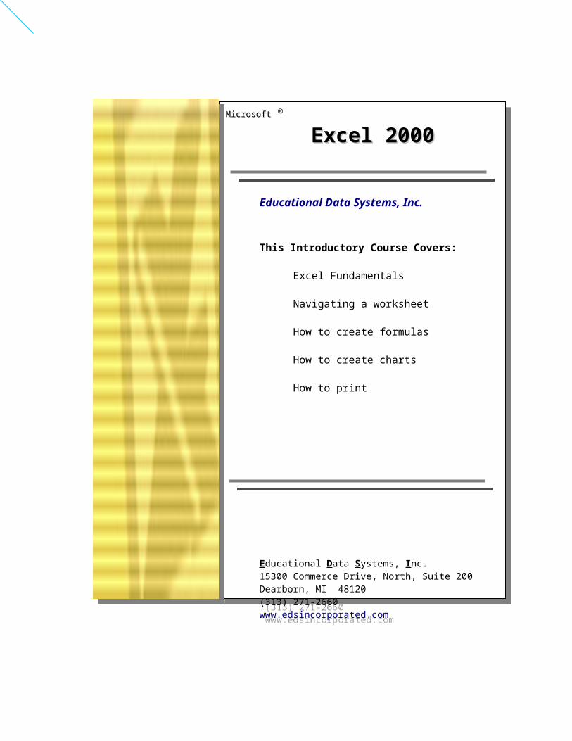
Table of ContentsTable of Contents
Chapter One: Chapter One: Excel FundamentalsExcel Fundamentals...............................................................................1Screen ElementsScreen Elements.......................................................................................................................2Excel Screen Elements.............................................................................................................3Title Bar....................................................................................................................................3
Using Menus........................................................................................................................................4
Using Toolbars...................................................................................................................................6Formatting Toolbar.............................................................................................................................7
Shortcuts..............................................................................................................................................8Keystroke Shortcuts..................................................................................................................8Function Keys...........................................................................................................................8
Common Menu / Toolbar Functions in Microsoft Office SuiteCommon Menu / Toolbar Functions in Microsoft Office Suite.................9
What are Workbooks and Worksheets?What are Workbooks and Worksheets?.................................................................10
Chapter Two: Navigating a WorksheetChapter Two: Navigating a Worksheet...................................................................12
Chapter Three: Entering Labels and Values in a WorksheetChapter Three: Entering Labels and Values in a Worksheet.................14Entering Repetitive Data Quickly...........................................................................................20
Sorting Data.................................................................................................................................24
Quiz 2....................................................................................................................................................26
Chapter Four: Formulas......................................................................................................27Basic Functions.......................................................................................................................27
Quiz 3....................................................................................................................................................32
Chapter Five: ChartsChapter Five: Charts..............................................................................................................33
Quiz 4...................................................................................................................................................36
Chapter Six: Saving Your Work.....................................................................................37
Guidelines for Naming WorkbooksGuidelines for Naming Workbooks.............................................................................38
The Importance of Planning Your WorkbookThe Importance of Planning Your Workbook.....................................................39
Prepare a Workbook to PrintPrepare a Workbook to Print..........................................................................................40Print Preview ....................................................................................................................40
When You Need HelpWhen You Need Help.............................................................................................................43
AppendixAppendix.........................................................................................................................................45Microsoft Excel Keyboard Shortcuts.........................................................................................46
Password Protect Cells, Worksheets, and FilesPassword Protect Cells, Worksheets, and Files...............................................49Customizing the Toolbar............................................................................................................50Searching for Help on the Web..................................................................................................52

Chapter One: Chapter One: Excel FundamentalsExcel FundamentalsBrief History of SpreadsheetsThe concept of spreadsheets has been around as long as business accounting practices have been around. Tables of rows and columns on paper were used to organize data for record keeping and analysis. As personal computers came along in the 1970’s, it became possible for programmers to eliminate many tedious and repetitive activities involved in managing paper spreadsheets. This also greatly improved accuracy.
A pair of graduate students became bored and frustrated with the tedium of such activities in their coursework, Dan Bricklin from Harvard and Robert Frankston from MIT. Out of that frustration Visicalc, the first spreadsheet, was born in 1978. The invention of the spreadsheet made personal computers have real value in the market place and legitimated the personal computer industry.
Today Excel software pretty much dominates the spreadsheet market. It is estimated that it has 90% of the market share. It allows you to create spreadsheet much like paper ledgers that can perform automatic calculations. Each Excel file is a workbook that can hold many worksheets. A worksheet is a grid of columns (designated by letters) and rows (designated by numbers).
Columns and Rows: The letter and numbers on the columns and rows (called labels) are displayed in gray buttons across the top and left side of the worksheet.
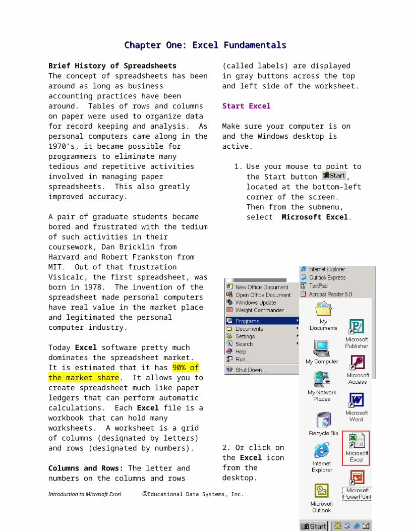
Start Excel
Make sure your computer is on and the Windows desktop is active.
1. Use your mouse to point to the Start button , located at the bottom-left corner of the screen. Then from the submenu, select Microsoft Excel.
2. Or click on the Excel icon from the desktop.
Introduction to Microsoft Excel Educational Data Systems, Inc. 1
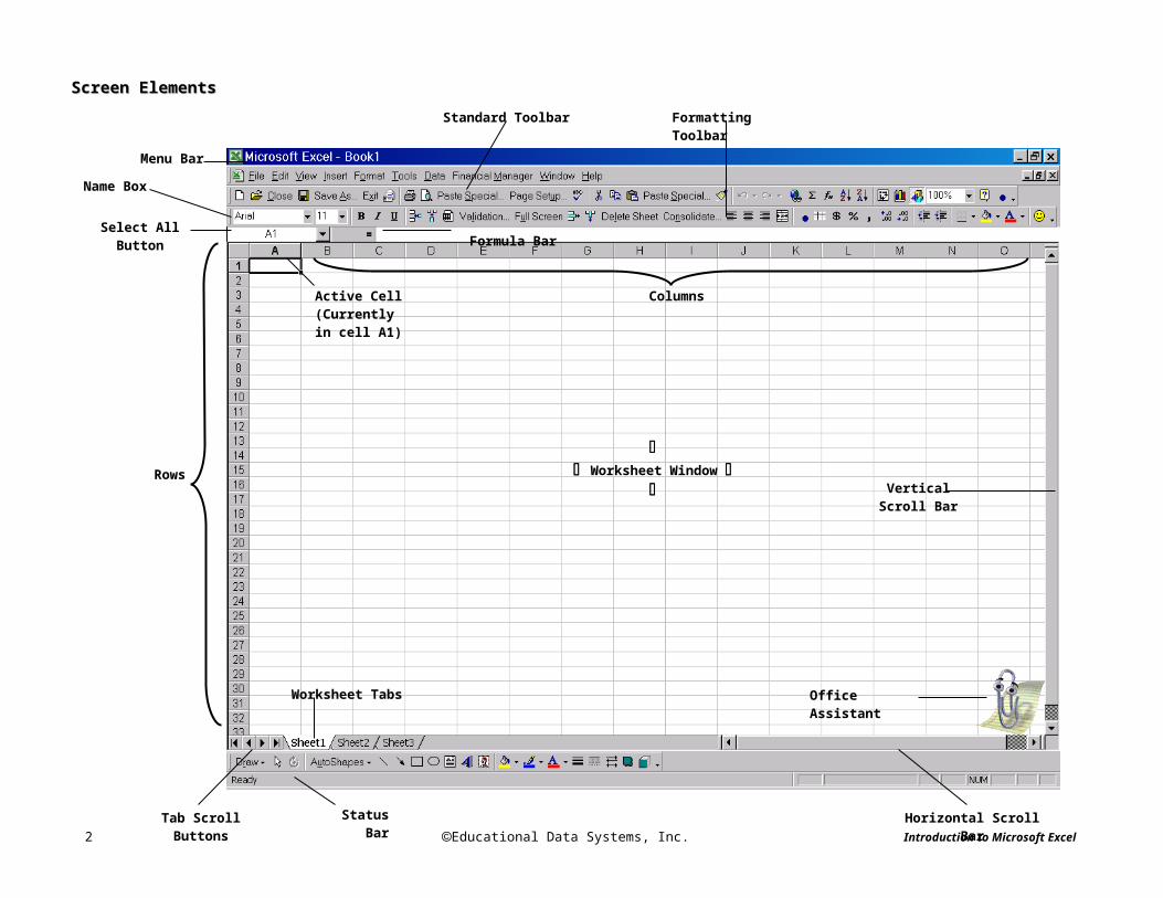
Screen ElementsScreen Elements
2 Educational Data Systems, Inc. Introduction to Microsoft Excel
Horizontal Scroll Bar
Menu Bar
Formatting ToolbarStandard Toolbar
Columns
Vertical Scroll Bar
Worksheet Window
Worksheet Tabs
Status Bar
Name Box
Select All Button
Tab Scroll Buttons
Office Assistant
Active Cell (Currently in cell A1)
Rows
Formula Bar

Excel Screen Elements
Element What It’s Used For
Title Bar Displays the name of the program you are currently using and the name of the workbook you are working on. The title bar appears at the top of all Windows programs.
Menu Bar Displays a list of menus you use to give commands to Excel. Clicking a menu name displays a list of commands; for example, clicking the Format menu name displays different formatting commands.
Standard Toolbar Toolbars are shortcuts; they contain icons for the most commonly used commands (instead of having to wade through several menus). The Standard toolbar contains buttons for the Excel commands you use the most, such as saving, opening, and printing workbooks.
Formatting Toolbar
Contains icons for the most commonly used formatting commands, such as making text bold or italicized.
Worksheet Window
This is where you enter data and work on your worksheets. You can have more than one worksheet window open at a time, allowing you to work on several worksheets.
Cell Pointer and Active Cell
Highlights the cell you are working on. The current cell in the sample above is located at A1. To make another cell active just click the cell with the mouse or press the arrow keys on the keyboard to move the cell pointer to the new location.
Formula Bar Allow you to view, enter, and edit data in the current cell. The Formula bar displays any formulas a cell might contain.
Name Box Displays active cell address. In the example above, “A1” appears in the name box, indicating that the active cell is A1.
Worksheet Tabs You can keep multiple worksheets together in a group called a workbook. You can move quickly from one worksheet to another by clicking the worksheet tabs. You can give worksheets your own meaningful names, such as “Budget” instead of “Sheet.” Excel workbooks contain 3 worksheets by default.
Scroll Bar These are both vertical and horizontal scroll bars; you use them to view and move around your spreadsheet. The scroll box shows where you are in the workbook; for example, if the scroll box is near the top of the scroll bar you’re at the beginning of the workbook.
Status Bar Displays messages and feedback.
Introduction to Microsoft Excel Educational Data Systems, Inc. 3
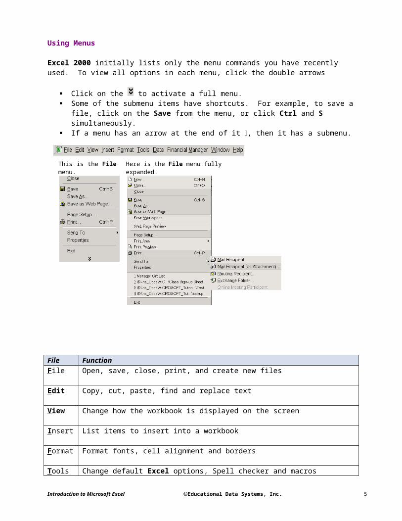
Using Menus
Excel 2000 initially lists only the menu commands you have recently used. To view all options in each menu, click the double arrows
Click on the to activate a full menu. Some of the submenu items have shortcuts. For example, to save a file, click on the
Save from the menu, or click Ctrl and S simultaneously. If a menu has an arrow at the end of it , then it has a submenu.
File FunctionFile Open, save, close, print, and create new files
Edit Copy, cut, paste, find and replace text
View Change how the workbook is displayed on the screen
Insert List items to insert into a workbook
Format Format fonts, cell alignment and borders
Tools Change default Excel options, Spell checker and macros
Data Analyze and work with data information
Window Display and arrange multiple windows
Help Get help with any Excel related items
4 Educational Data Systems, Inc. Introduction to Microsoft Excel
Here is the File menu fully expanded.This is the File menu.

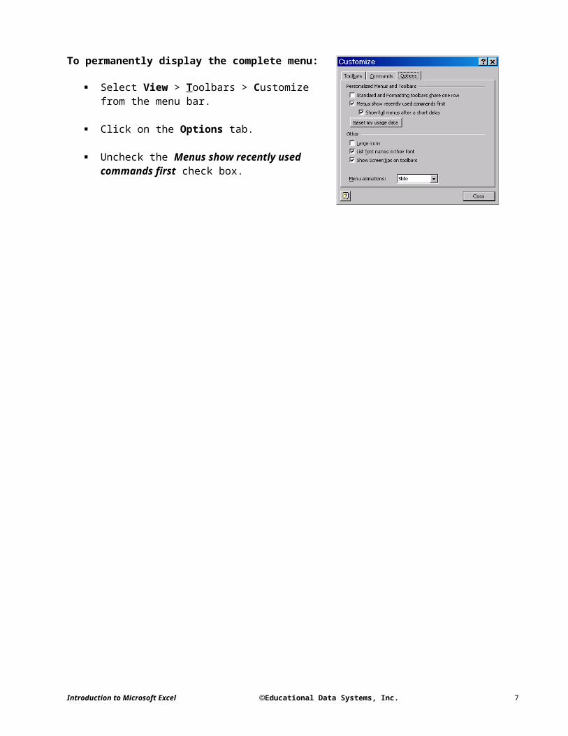
To permanently display the complete menu:
Select View > Toolbars > Customize from the menu bar.
Click on the Options tab.
Uncheck the Menus show recently used commands first check box.
Introduction to Microsoft Excel Educational Data Systems, Inc. 5

Using Toolbars
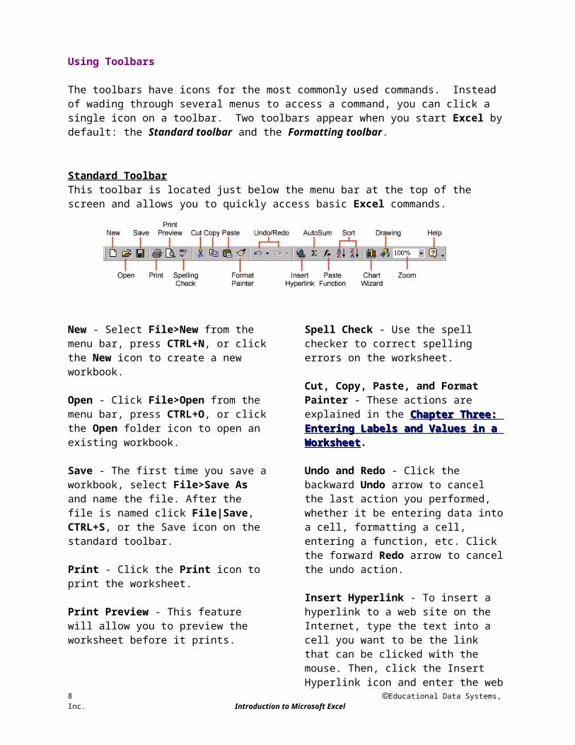
The toolbars have icons for the most commonly used commands. Instead of wading through several menus to access a command, you can click a single icon on a toolbar. Two toolbars appear when you start Excel by default: the Standard toolbar and the Formatting toolbar.
Standard ToolbarThis toolbar is located just below the menu bar at the top of the screen and allows you to quickly access basic Excel commands.
New - Select File>New from the menu bar, press CTRL+N, or click the New icon to create a new workbook.
Open - Click File>Open from the menu bar, press CTRL+O, or click the Open folder icon to open an existing workbook.
Save - The first time you save a workbook, select File>Save As and name the file. After the file is named click File|Save, CTRL+S, or the Save icon on the standard toolbar.
Print - Click the Print icon to print the worksheet.
Print Preview - This feature will allow you to preview the worksheet before it prints.
Spell Check - Use the spell checker to correct spelling errors on the worksheet.
Cut, Copy, Paste, and Format Painter - These actions are explained in the Chapter Chapter
Three: Entering Labels and Values in a Three: Entering Labels and Values in a WorksheetWorksheet.
Undo and Redo - Click the backward Undo arrow to cancel the last action you performed, whether it be entering data into a cell, formatting a cell, entering a function, etc. Click the forward Redo arrow to cancel the undo action.
Insert Hyperlink - To insert a hyperlink to a web site on the Internet, type the text into a cell you want to be the link that can be clicked with the mouse. Then, click the Insert Hyperlink icon and enter the web address you want the text to link to and click OK.
Autosum, Function Wizard, and Sorting - These features are discussed in detail in Chapter Four: FormulasChapter Four: Formulas.
Zoom - To change the size that the worksheet appears on the screen, choose a different percentage from the Zoom menu.
6 Educational Data Systems, Inc. Introduction to Microsoft Excel

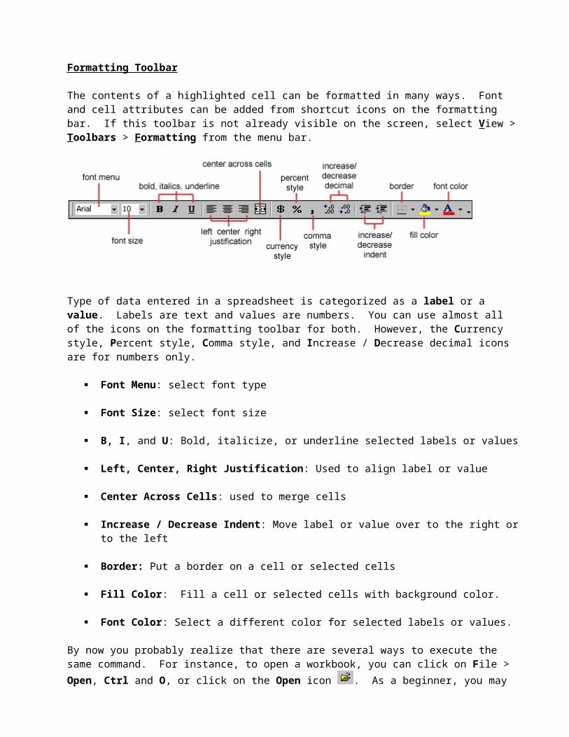
Formatting Toolbar
The contents of a highlighted cell can be formatted in many ways. Font and cell attributes can be added from shortcut icons on the formatting bar. If this toolbar is not already visible on the screen, select View > Toolbars > Formatting from the menu bar.
Type of data entered in a spreadsheet is categorized as a label or a value. Labels are text and values are numbers. You can use almost all of the icons on the formatting toolbar for both. However, the Currency style, Percent style, Comma style, and Increase / Decrease decimal icons are for numbers only.
Font Menu: select font type
Font Size: select font size
B, I, and U: Bold, italicize, or underline selected labels or values
Left, Center, Right Justification: Used to align label or value
Center Across Cells: used to merge cells
Increase / Decrease Indent: Move label or value over to the right or to the left
Border: Put a border on a cell or selected cells
Fill Color: Fill a cell or selected cells with background color.
Font Color: Select a different color for selected labels or values.
By now you probably realize that there are several ways to execute the same command. For instance, to open a workbook, you can click on File > Open, Ctrl and O, or click on the Open icon
. As a beginner, you may find this confusing. However, opting to use the menu as opposed to the shortcuts is a matter of personal preference. Please feel free to use the option most convenient for you!
Shortcuts
Keystroke Shortcuts
You can combine the Alt, Ctrl, and Shift keys with keyboard letters to perform a multitude of shortcuts. For instance, you can save your workbook by pressing Ctrl and S simultaneously.
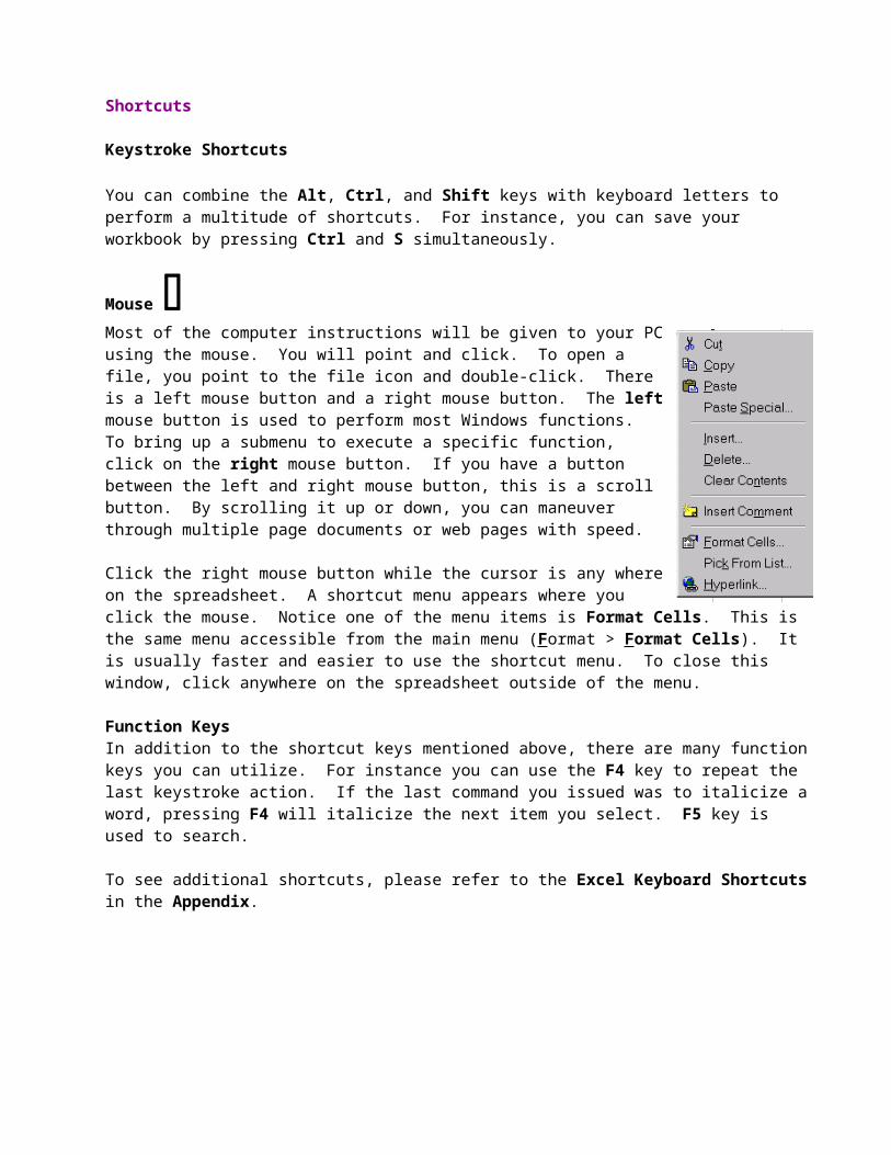
Mouse Most of the computer instructions will be given to your PC using the mouse. You will point and click. To open a file, you point to the file icon and double-click. There is a left mouse button and a right mouse button. The left mouse button is used to perform most Windows functions. To bring up a submenu to execute a specific function, click on the right mouse button. If you have a button between the left and right mouse button, this is a scroll button. By scrolling it up or down, you can maneuver through multiple page documents or web pages with speed.
Click the right mouse button while the cursor is any where on the spreadsheet. A shortcut menu appears where you click the mouse. Notice one of the menu items is Format Cells. This is the same menu accessible from the main menu (Format > Format Cells). It is usually faster and easier to use the shortcut menu. To close this window, click anywhere on the spreadsheet outside of the menu.
Function KeysIn addition to the shortcut keys mentioned above, there are many function keys you can utilize. For instance you can use the F4 key to repeat the last keystroke action. If the last command you issued was to italicize a word, pressing F4 will italicize the next item you select. F5 key is used to search.
To see additional shortcuts, please refer to the Excel Keyboard Shortcuts in the Appendix.
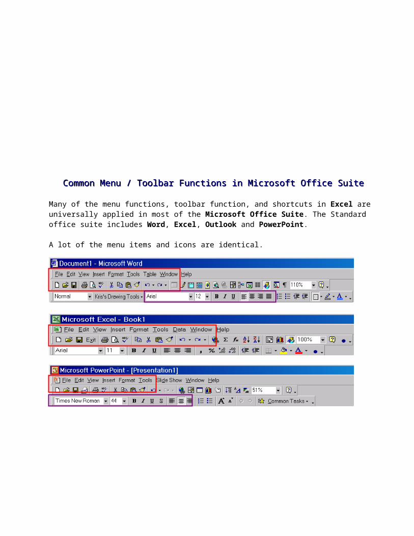
Common Menu / Toolbar Functions in Microsoft Office SuiteCommon Menu / Toolbar Functions in Microsoft Office SuiteMany of the menu functions, toolbar function, and shortcuts in Excel are universally applied in most of the Microsoft Office Suite. The Standard office suite includes Word, Excel, Outlook and PowerPoint.
A lot of the menu items and icons are identical.

What are Workbooks and Worksheets?What are Workbooks and Worksheets?
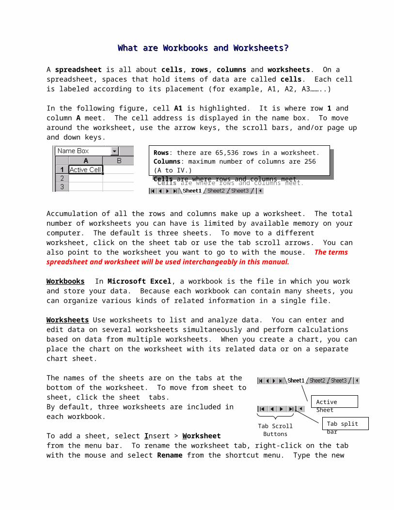
A spreadsheet is all about cells, rows, columns and worksheets. On a spreadsheet, spaces that hold items of data are called cells. Each cell is labeled according to its placement (for example, A1, A2, A3……..)
In the following figure, cell A1 is highlighted. It is where row 1 and column A meet. The cell address is displayed in the name box. To move around the worksheet, use the arrow keys, the scroll bars, and/or page up and down keys.
Accumulation of all the rows and columns make up a worksheet. The total number of worksheets you can have is limited by available memory on your computer. The default is three sheets. To move to a different worksheet, click on the sheet tab or use the tab scroll arrows. You can also point to the worksheet you want to go to with the mouse. The terms spreadsheet and worksheet will be used interchangeably in this manual.
Workbooks In Microsoft Excel, a workbook is the file in which you work and store your data. Because each workbook can contain many sheets, you can organize various kinds of related information in a single file.
Worksheets Use worksheets to list and analyze data. You can enter and edit data on several worksheets simultaneously and perform calculations based on data from multiple worksheets. When you create a chart, you can place the chart on the worksheet with its related data or on a separate chart sheet.
The names of the sheets are on the tabs at the bottom of the worksheet. To move from sheet to sheet, click the sheet tabs. By default, three worksheets are included in each workbook.
To add a sheet, select Insert > Worksheet from the menu bar. To rename the worksheet tab, right-click on the tab with the mouse and select Rename from the shortcut menu. Type the new name and press the ENTER key. Alternatively, you can double-click on it and change the name.
Cell Range The data area on a spreadsheet is called a cell range. It is also called a data range. If you enter data from cell A1 to cell C5, cells A1, A2, A3, A4, A5, B1, B2, B3, B4, B5, C1, C2, C3, C4, and C5 is your cell range. It’s very important that you understand this concept!
Rows: there are 65,536 rows in a worksheet.Columns: maximum number of columns are 256 (A to IV.)Cells are where rows and columns meet.
Active Sheet
Tab Scroll Buttons Tab split bar

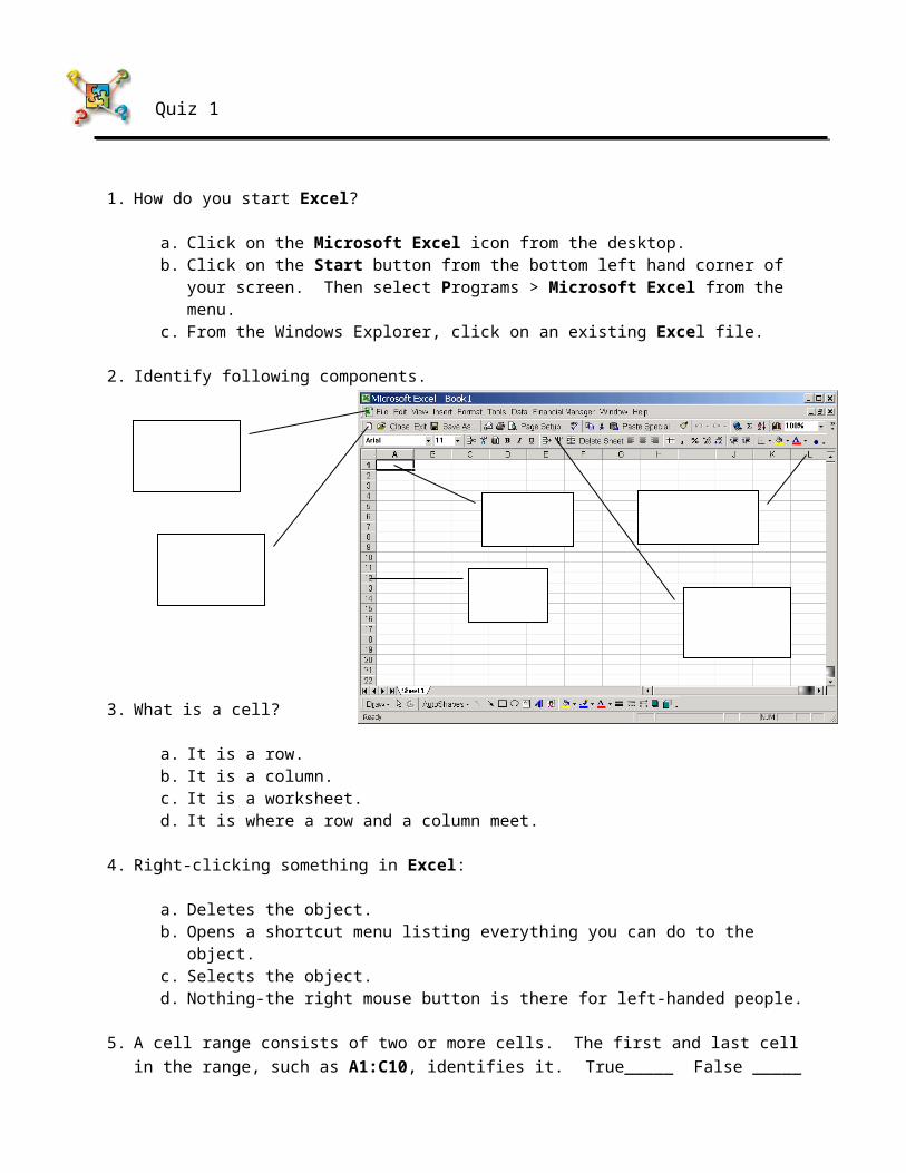
Quiz 1
1. How do you start Excel?
a. Click on the Microsoft Excel icon from the desktop.b. Click on the Start button from the bottom left hand corner of your screen. Then select
Programs > Microsoft Excel from the menu.c. From the Windows Explorer, click on an existing Excel file.
2. Identify following components.
3. What is a cell?
a. It is a row.b. It is a column.c. It is a worksheet.d. It is where a row and a column meet.
4. Right-clicking something in Excel:
a. Deletes the object.b. Opens a shortcut menu listing everything you can do to the object.c. Selects the object.d. Nothing-the right mouse button is there for left-handed people.
5. A cell range consists of two or more cells. The first and last cell in the range, such as A1:C10, identifies it. True_____ False _____
6. To save a workbook:
a. Press Ctrl + S.b. Select File > Save from the menu.c. Click the Save icon from the standard toolbar. Exit from Excel.
Chapter Two: Navigating a WorksheetChapter Two: Navigating a Worksheet
There are many ways you can move around the spreadsheet. You can use the Page Up or Page Down keys. Or you can scroll up, down, across using your mouse. When you have a big spreadsheet, it will be very helpful to know how to get around a spreadsheet fast.
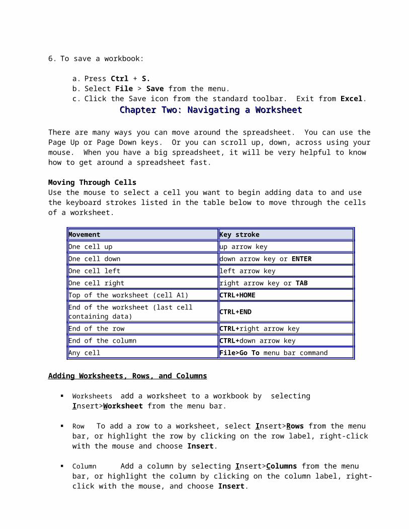
Moving Through CellsUse the mouse to select a cell you want to begin adding data to and use the keyboard strokes listed in the table below to move through the cells of a worksheet.
Movement Key strokeOne cell up up arrow keyOne cell down down arrow key or ENTEROne cell left left arrow keyOne cell right right arrow key or TABTop of the worksheet (cell A1) CTRL+HOMEEnd of the worksheet (last cell containing data) CTRL+ENDEnd of the row CTRL+right arrow keyEnd of the column CTRL+down arrow keyAny cell File>Go To menu bar command
Adding Worksheets, Rows, and Columns
Worksheets add a worksheet to a workbook by selecting Insert>Worksheet from the menu bar.
Row To add a row to a worksheet, select Insert>Rows from the menu bar, or highlight the row by clicking on the row label, right-click with the mouse and choose Insert.
Column Add a column by selecting Insert>Columns from the menu bar, or highlight the column by clicking on the column label, right-click with the mouse, and choose Insert.
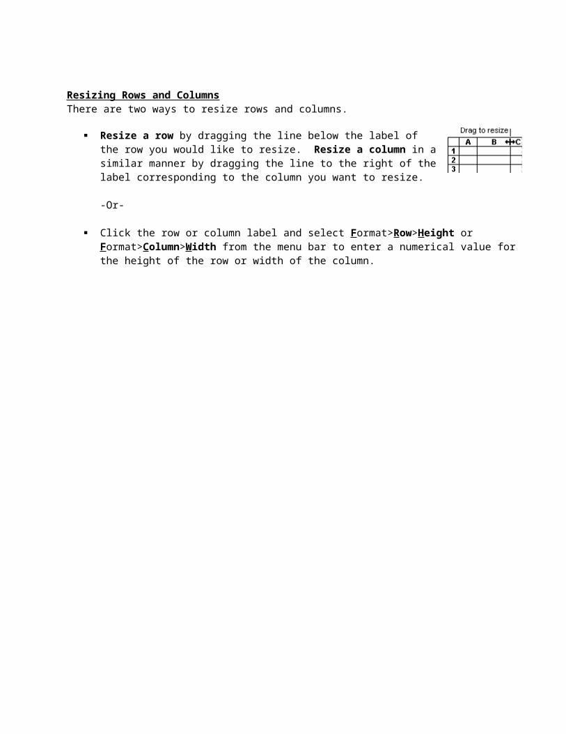
Resizing Rows and ColumnsThere are two ways to resize rows and columns.
Resize a row by dragging the line below the label of the row you would like to resize. Resize a column in a similar manner by dragging the line to the right of the label corresponding to the column you want to resize.
-Or-
Click the row or column label and select Format>Row>Height or Format>Column>Width from the menu bar to enter a numerical value for the height of the row or width of the column.

Selecting CellsBefore a cell can be modified or formatted, it must first be selected (highlighted). Refer to the table below for selecting groups of cells.
Cells to select Mouse actionOne cell Click once in the cellEntire row Click the row labelEntire column Click the column labelEntire worksheet Click the whole sheet button
Cluster of cells Drag mouse over the cells or hold down the SHIFT key while using the arrow keys
To edit a cell, double-click on the cell or click once and press F2.
Moving and Copying Cells
Moving Cells To cut cell contents, highlight the cell(s) and select Edit>Cut from the menu bar or click the cut button on the standard toolbar or press Ctrl and X.
Pasting Cut and Copied Cells Highlight the cells(s) you want to paste the cut or copied contents into and select Edit>Paste from the menu bar or click the Paste icon on the standard toolbar or press Ctrl and V.
Copying Cells To copy the cell contents, highlight the cell(s) and select Edit>Copy from the menu bar or click the Copy button on the standard toolbar or press Ctrl and C.
Drag and DropIf you are moving the cell contents only a short distance, the drag-and-drop method may be easier. Simply drag the highlighted border of the selected cell to the destination cell with the mouse.
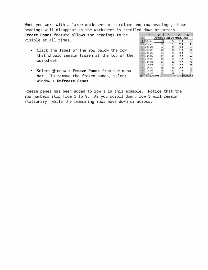
Freeze PanesWhen you work with a large worksheet with column and row headings, those headings will disappear as the worksheet is scrolled down or across. Freeze Panes feature allows the headings to be visible at all times.
Click the label of the row below the row that should remain frozen at the top of the worksheet.
Select Window > Freeze Panes from the menu bar. To remove the frozen panes, select Window > Unfreeze Panes.
Freeze panes has been added to row 1 in this example. Notice that the row numbers skip from 1 to 9. As you scroll down, row 1 will remain stationary, while the remaining rows move down or across.
Chapter Three: Entering Labels and Values in a WorksheetChapter Three: Entering Labels and Values in a Worksheet
There are two basic types of data you can enter in a cell:
Labels: Any type of text or information not used in any calculations.Values: Any type of numerical data, numbers, percentages, fractions, currencies, dates, times, usually used in formulas or calculations.
Let’s Practice!Basically labels are used in worksheets for headings and make your worksheets easy to read and understand. Let’s create a simple spreadsheet.
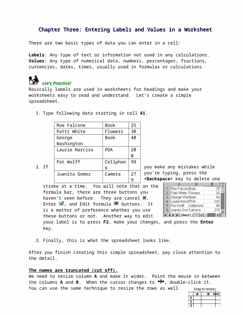
1. Type following data starting in cell A1.
2. If you make any mistakes while you’re typing, press the <Backspace> key to delete one stroke at a time. You will note that on the formula bar, there are three buttons you haven’t seen before. They are cancel , Enter , and Edit formula buttons. It is a matter of preference whether you use these buttons or not. Another way to edit your label is to press F2, make your changes, and press the Enter key.
3. Finally, this is what the spreadsheet looks like.
After you finish creating this simple spreadsheet, pay close attention to the detail.
The names are truncated (cut off).We need to resize column A and make it wider. Point the mouse in between the columns A and B. When the cursor changes to , double-click it. You can use the same technique to resize the rows as well.
If you have a large spreadsheet, you can click on the select all button and highlight the entire worksheet. Then click in between the columns or rows to let Excel find the automatic fit for the entire spreadsheet.
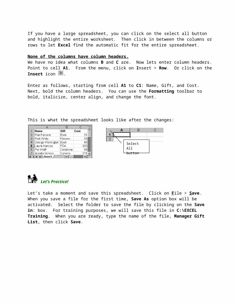
None of the columns have column headers.We have no idea what columns B and C are. Now lets enter column headers. Point to cell A1. From the menu, click on Insert > Row. Or click on the Insert icon .
Enter as follows, starting from cell A1 to C1: Name, Gift, and Cost. Next, bold the column headers. You can use the Formatting toolbar to bold, italicize, center align, and change the font.
Roe Falcone Book 25Patti White Flowers 30George Washington Book 40Laurie Narciso PDA 200Pat Wolff Cellphone 99Juanita Gomez Camera 279
This is what the spreadsheet looks like after the changes:
Let’s Practice!
Let’s take a moment and save this spreadsheet. Click on File > Save. When you save a file for the first time, Save As option box will be activated. Select the folder to save the file by clicking on the Save in: box. For training purposes, we will save this file in C:\EXCEL Training. When you are ready, type the name of the file, Manager Gift List, then click Save.
Select All button
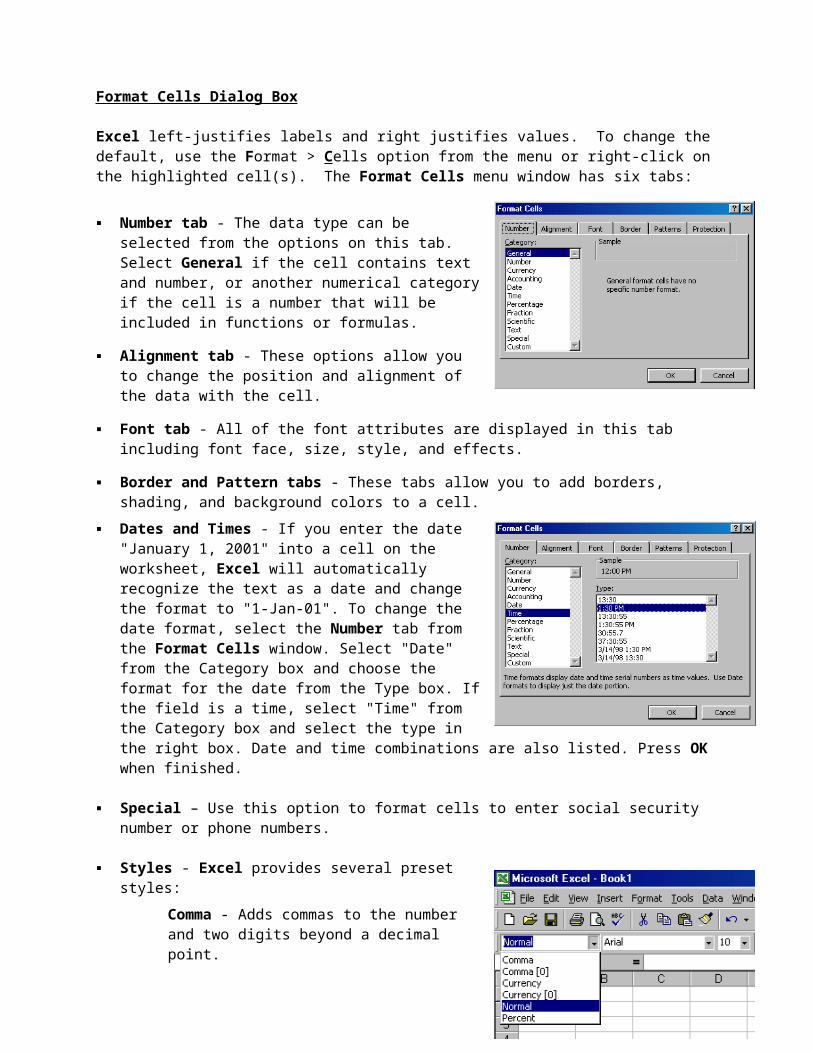
Format Cells Dialog Box
Excel left-justifies labels and right justifies values. To change the default, use the Format > Cells option from the menu or right-click on the highlighted cell(s). The Format Cells menu window has six tabs:
Number tab - The data type can be selected from the options on this tab. Select General if the cell contains text and number, or another numerical category if the cell is a number that will be included in functions or formulas.
Alignment tab - These options allow you to change the position and alignment of the data with the cell.
Font tab - All of the font attributes are displayed in this tab including font face, size, style, and effects.
Border and Pattern tabs - These tabs allow you to add borders, shading, and background colors to a cell.
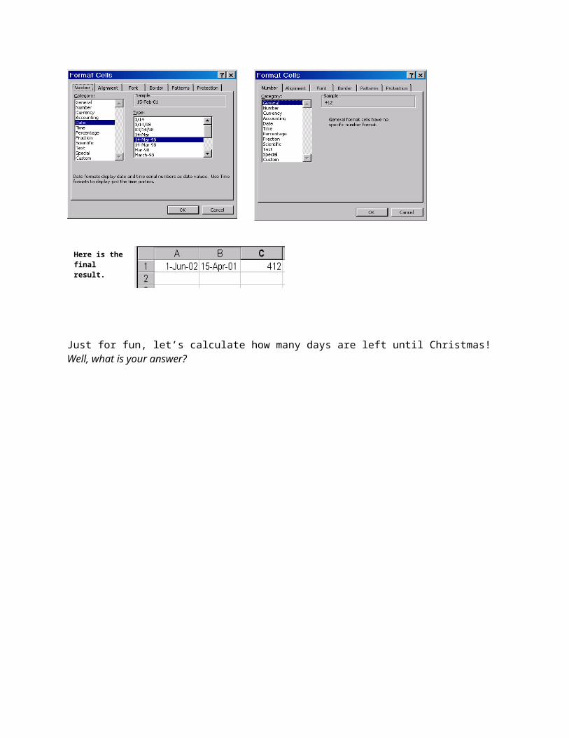
Dates and Times - If you enter the date "January 1, 2001" into a cell on the worksheet, Excel will automatically recognize the text as a date and change the format to "1-Jan-01". To change the date format, select the Number tab from the Format Cells window. Select "Date" from the Category box and choose the format for the date from the Type box. If the field is a time, select "Time" from the Category box and select the type in the right box. Date and time combinations are also listed. Press OK when finished.
Special – Use this option to format cells to enter social security number or phone numbers.
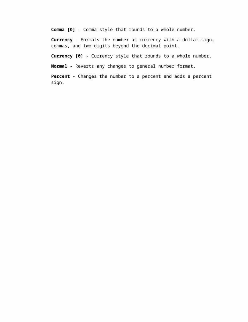
Styles - Excel provides several preset styles:Comma - Adds commas to the number and two digits beyond a decimal point.
Comma [0] - Comma style that rounds to a whole number.
Currency - Formats the number as currency with a dollar sign, commas, and two digits beyond the decimal point.
Currency [0] - Currency style that rounds to a whole number.
Normal - Reverts any changes to general number format.
Percent - Changes the number to a percent and adds a percent sign.

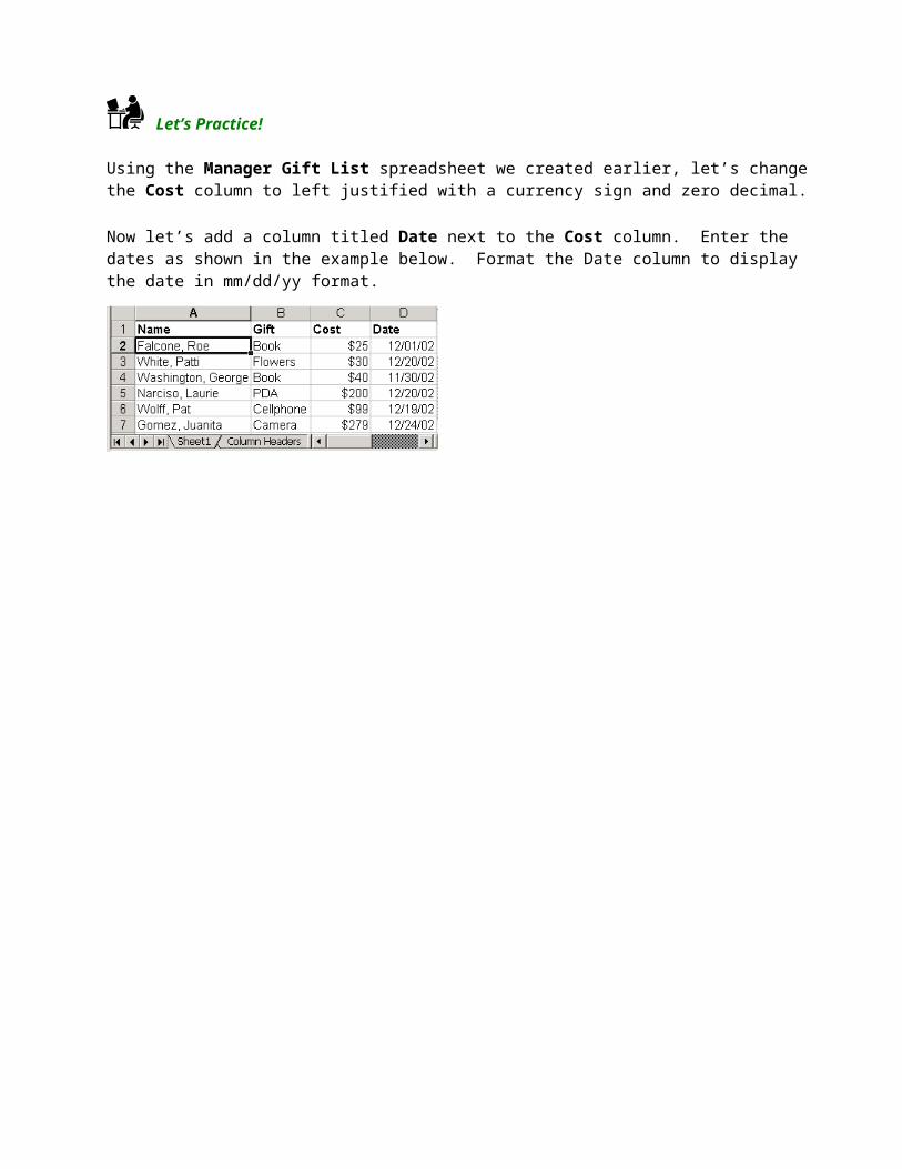
Let’s Practice!
Using the Manager Gift List spreadsheet we created earlier, let’s change the Cost column to left justified with a currency sign and zero decimal.
Now let’s add a column titled Date next to the Cost column. Enter the dates as shown in the example below. Format the Date column to display the date in mm/dd/yy format.
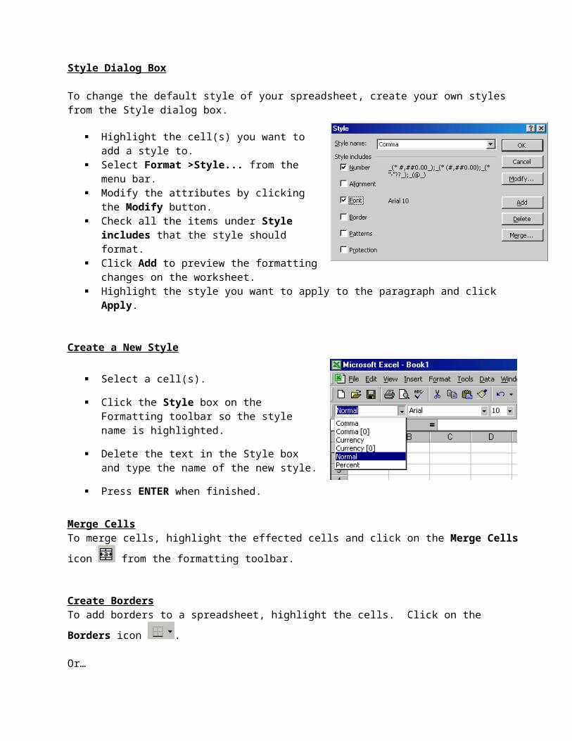
Style Dialog Box
To change the default style of your spreadsheet, create your own styles from the Style dialog box.
Highlight the cell(s) you want to add a style to. Select Format >Style... from the menu bar. Modify the attributes by clicking the Modify
button. Check all the items under Style includes that
the style should format. Click Add to preview the formatting changes on
the worksheet. Highlight the style you want to apply to the
paragraph and click Apply.
Create a New Style
Select a cell(s).
Click the Style box on the Formatting toolbar so the style name is highlighted.
Delete the text in the Style box and type the name of the new style.
Press ENTER when finished.
Merge Cells
To merge cells, highlight the effected cells and click on the Merge Cells icon from the formatting toolbar.
Create Borders
To add borders to a spreadsheet, highlight the cells. Click on the Borders icon .
Or…
Select Format > Cells and select the Borders tab
Or…
Press the Ctrl + 1 simultaneously
Format Painter A handy feature on the standard toolbar for formatting text is the Format Painter. If you have formatted a cell with a certain font style, date format, border, and other formatting options, and you want to format another cell or group of cells the same way, place the cursor within the cell containing the formatting you want to copy. Click the Format Painter button in the standard toolbar (notice that your pointer now has a paintbrush beside it). Highlight the cells you want to add the same formatting to.
To copy the formatting to many groups of cells, double-click the Format Painter button. The format painter remains active until you press the ESC key to turn it off.
AutoFormat
Excel has many preset table formatting options. Add these styles by following these steps:
Highlight the cells that will be formatted.
Select Format>AutoFormat from the menu bar.
On the AutoFormat dialog box, select the format you want to apply to the table by clicking on it with the mouse. Use the scroll bar to view all of the formats available.
Click on the Options... button to select the elements that the formatting will apply to.
Click OK when finished. The distinguishing feature of a spreadsheet program such as Excel is that it allows you to create mathematical formulas and execute functions. Otherwise, it is not much more than a large table for displaying text.
Entering Repetitive Data Quickly
If you need to type repetitive data such as numbers or dates into a spreadsheet, you can use the AutoFill feature in Excel to help you. Here's an exercise:
Let’s Practice!First, fill a group of cells with the names of the calendar months:
Start Excel. A new, blank workbook appears. In cell A1, type January and then press ENTER.
Click anywhere inside cell A1, and rest the mouse pointer on the square at the lower right-hand corner of cell A1. The mouse pointer changes into a plus symbol (+). Press and hold the right mouse button, drag the mouse pointer to cell A12 and release the right mouse button.
A menu appears. Click Fill Months. The names of the months February, March, and so on appear in cells A2 through A12.
Next, quickly fill in several cells with the same value:
In cell B1, type 1999 and press ENTER. Click anywhere inside of cell B1, and rest the mouse pointer on the fill handle at the lower right-hand corner of cell B1. The mouse pointer changes to a plus symbol (+). Press and hold the right mouse button, drag the mouse pointer to cell B12, and release the right mouse button. A menu appears. Click Copy Cells. The value 1999 appears in cells B2 though B12.
There is even a quicker way to do copy labels and formulas. When the mouse pointer changes to a plus sign
, double-click with the left mouse button.

Finally, quickly fill in several cells with a range of numbers:
In cell C1, type 10000. Click anywhere inside of cell C1, and rest the mouse pointer on the square at the lower right-hand corner of cell C1. The mouse pointer changes into a plus symbol (+).
Press and hold the right mouse button, drag the mouse pointer to cell C12 and release the right mouse button. A menu appears. Click Series.
In the Step value box, type 125, and click OK. The Series dialog box disappears, the value 10125 appears in cell C2, and the number increments by 125 in each cell in column C up to an ending value of 11375 in cell C12.
Here is the final result.
Transposing Data
Once in a while, you have to turning things around!
Let’s Practice!What I mean is your rows and columns… Let’s assume that we want to switch the columns and rows. That is what transposing means. Create a spreadsheet that looks like the example below. When you are finished, start dragging your mouse from cell A1 to cell D4. Remember the cell range?
Then, click Copy icon or press Ctrl + C.
Click anywhere on the worksheet, that is excluding the cell range with the original data. From the menu, select Edit > Paste Special. Next, select Transpose and click OK.
Finally, click on the Paste icon or press Ctrl + V.
Before
After
View multiple sheets or workbooks at the same time
Open the workbooks you want to view. On the Window menu, click Arrange and select the option you want.
To view sheets on the active workbook, select the Windows of active workbook check box.
To restore a workbook window to full size, click on the Maximize button at the upper-right corner of the workbook window.
To view multiple sheets from the same workbook, click New Window on the Window menu. Switch to the new window, and then click a sheet you want to view. Resize the window to fit as many as you like.
Sorting Data
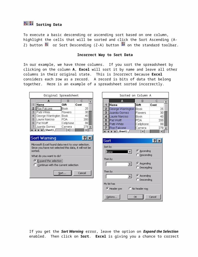
To execute a basic descending or ascending sort based on one column, highlight the cells that will be sorted and click the Sort Ascending (A-Z) button or Sort Descending (Z-A) button on the standard toolbar.
Incorrect Way to Sort Data
In our example, we have three columns. If you sort the spreadsheet by clicking on the column A, Excel will sort it by name and leave all other columns in their original state. This is Incorrect because Excel considers each row as a record. A record is bits of data that belong together. Here is an example of a spreadsheet sorted incorrectly.
If you get the Sort Warning error, leave the option on Expand the Selection enabled. Then click on Sort. Excel is giving you a chance to correct the sort error. If you chose the second option, click on the Undo icon to go back to the original view of the spreadsheet.
If you sort a spreadsheet incorrectly, you can do some damage. The type of damage depends on the size of the spreadsheet. If you don’t have a backup, there is no other way to get around it. You will simply have to retype everything. Imagine recreating a workbook that has thousands of records. It could take days if not weeks!
Original Spreadsheet Sorted on Column A

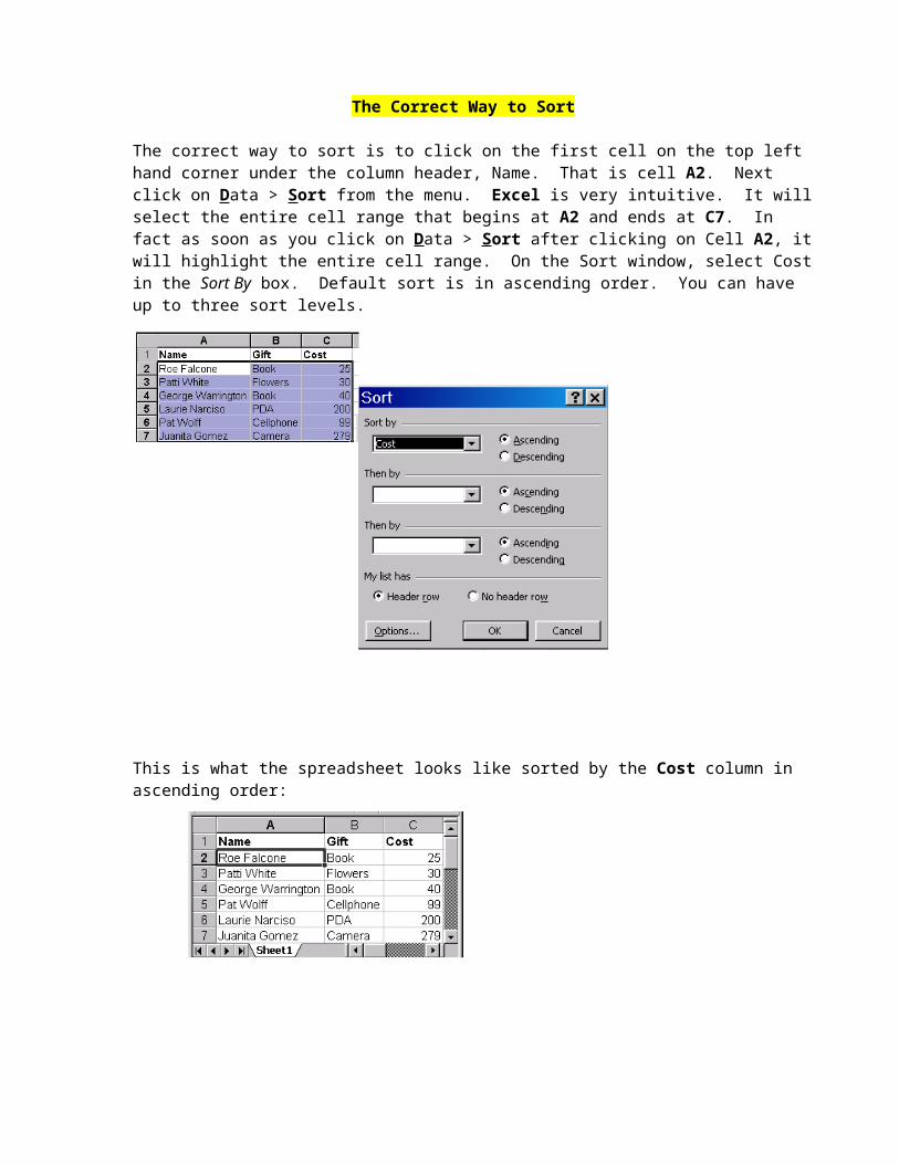
The Correct Way to Sort
The correct way to sort is to click on the first cell on the top left hand corner under the column header, Name. That is cell A2. Next click on Data > Sort from the menu. Excel is very intuitive. It will select the entire cell range that begins at A2 and ends at C7. In fact as soon as you click on Data > Sort after clicking on Cell A2, it will highlight the entire cell range. On the Sort window, select Cost in the Sort By box. Default sort is in ascending order. You can have up to three sort levels.
This is what the spreadsheet looks like sorted by the Cost column in ascending order:
Quiz 2
1. What is a label? ______________________________________________________________
What is a value? _______________________________________________________________
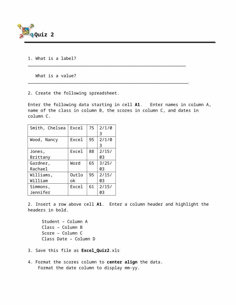
2. Create the following spreadsheet.
Enter the following data starting in cell A1. Enter names in column A, name of the class in column B, the scores in column C, and dates in column C.
Smith, Chelsea Excel 75 2/1/03Wood, Nancy Excel 95 2/1/03Jones, Brittany Excel 88 2/15/03Gardner, Rachael Word 65 3/25/03Williams, William Outlook 95 2/15/03Simmons, Jennifer Excel 61 2/15/03
2. Insert a row above cell A1. Enter a column header and highlight the headers in bold.
Student – Column AClass – Column BScore – Column CClass Date – Column D
3. Save this file as Excel_Quiz2.xls
4. Format the scores column to center align the data. Format the date column to display mm-yy.
5. Sort the spreadsheet by Class, Class Date, and Test Score in ascending order.
6. Open Excel_Quiz2.xls
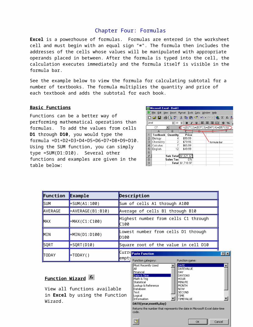
Chapter Four: FormulasExcel is a powerhouse of formulas. Formulas are entered in the worksheet cell and must begin with an equal sign "=". The formula then includes the addresses of the cells whose values will be manipulated with appropriate operands placed in between. After the formula is typed into the cell, the calculation executes immediately and the formula itself is visible in the formula bar.
See the example below to view the formula for calculating subtotal for a number of textbooks. The formula multiplies the quantity and price of each textbook and adds the subtotal for each book.
Basic Functions Functions can be a better way of performing mathematical operations than formulas. To add the values from cells D1 through D10, you would type the formula =D1+D2+D3+D4+D5+D6+D7+D8+D9+D10. Using the SUM function, you can simply type =SUM(D1:D10). Several other functions and examples are given in the table below:
Function Example DescriptionSUM =SUM(A1:100) Sum of cells A1 through A100AVERAGE =AVERAGE(B1:B10) Average of cells B1 through B10MAX =MAX(C1:C100) Highest number from cells C1 through C100MIN =MIN(D1:D100) Lowest number from cells D1 through D100SQRT =SQRT(D10) Square root of the value in cell D10TODAY =TODAY() Current date (leave the parentheses empty)
Function Wizard
View all functions available in Excel by using the Function Wizard.
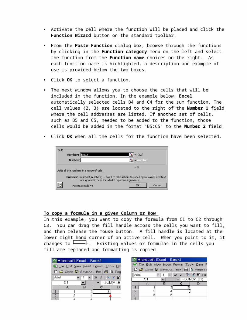
Activate the cell where the function will be placed and click the Function Wizard button on the standard toolbar.
From the Paste Function dialog box, browse through the functions by clicking in the Function category menu on the left and select the function from the Function name choices on the right. As each function name is highlighted, a description and example of use is provided below the two boxes.
Click OK to select a function.
The next window allows you to choose the cells that will be included in the function. In the example below, Excel automatically selected cells B4 and C4 for the sum function. The cell values {2, 3} are located to the right of the Number 1 field where the cell addresses are listed. If another set of cells, such as B5 and C5, needed to be added to the function, those cells would be added in the format "B5:C5" to the Number 2 field.
Click OK when all the cells for the function have been selected.
To copy a formula in a given Column or Row In this example, you want to copy the formula from C1 to C2 through C3. You can drag the fill handle across the cells you want to fill, and then release the mouse button. A fill handle is located at the lower right hand corner of an active cell. When you point to it, it changes to
. Existing values or formulas in the cells you fill are replaced and formatting is copied.
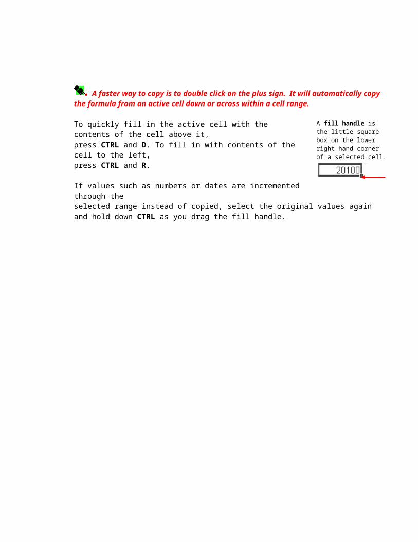
A faster way to copy is to double click on the plus sign. It will automatically copy the formula from an active cell down or across within a cell range.
To quickly fill in the active cell with the contents of the cell above it,press CTRL and D. To fill in with contents of the cell to the left, press CTRL and R.
If values such as numbers or dates are incremented through the selected range instead of copied, select the original values again and hold down CTRL as you drag the fill handle.
A fill handle is the little square box on the lower right hand corner of a selected cell.
If the fill handle is missing,On the Tools menu, click Options, click the Edit tab, and then make sure the Allow cell drag and drop check box is selected. If the entire row or column is selected, Microsoft Excel displays the fill handle at the beginning of the row or column.
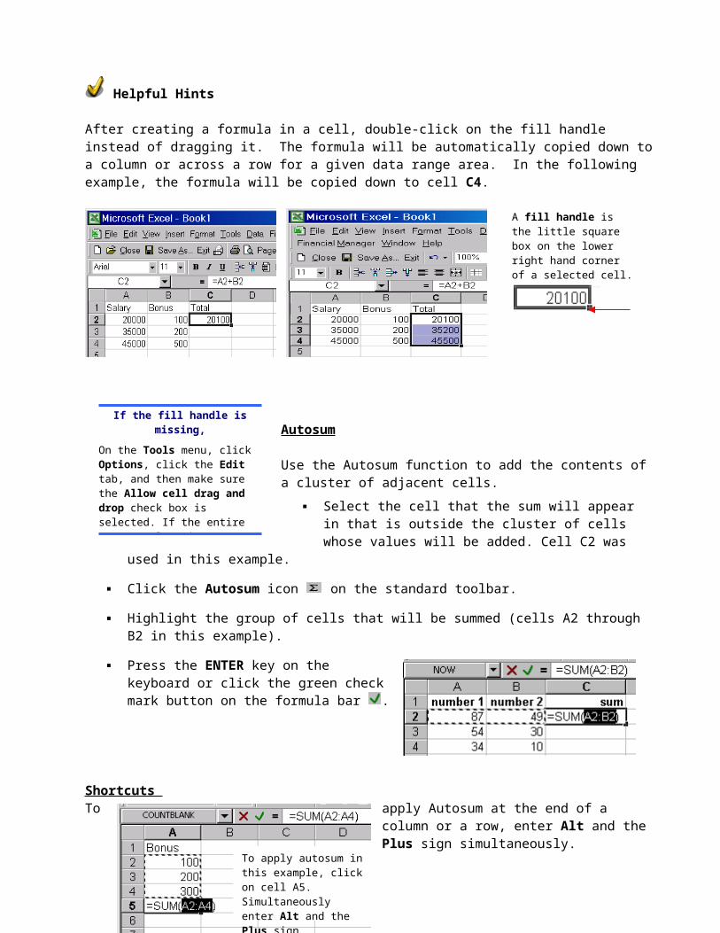
Helpful Hints
After creating a formula in a cell, double-click on the fill handle instead of dragging it. The formula will be automatically copied down to a column or across a row for a given data range area. In the following example, the formula will be copied down to cell C4.
Autosum
Use the Autosum function to add the contents of a cluster of adjacent cells. Select the cell that the sum will appear in that is outside the cluster of
cells whose values will be added. Cell C2 was used in this example.
Click the Autosum icon on the standard toolbar.
Highlight the group of cells that will be summed (cells A2 through B2 in this example).
Press the ENTER key on the keyboard or click the green check mark button on the formula bar .
Shortcuts To apply Autosum at the end of a column or a row, enter Alt and the Plus sign simultaneously.
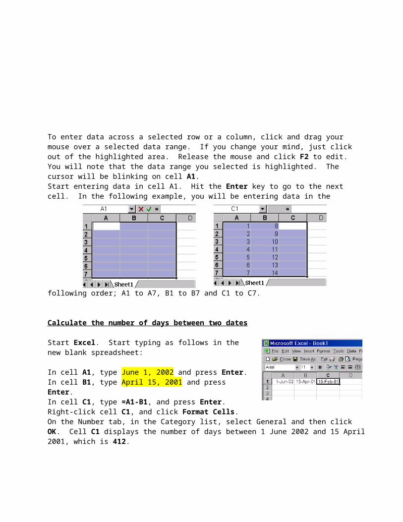
To enter data across a selected row or a column, click and drag your mouse over a selected data range. If you change your mind, just click out of the highlighted area. Release the mouse and click F2 to edit. You will note that the data range you selected is highlighted. The cursor will be blinking on cell A1.
To apply autosum in this example, click on cell A5. Simultaneously enter Alt and the Plus sign.
A fill handle is the little square box on the lower right hand corner of a selected cell.

Start entering data in cell A1. Hit the Enter key to go to the next cell. In the following example, you will be entering data in the following order; A1 to A7, B1 to B7 and C1 to C7.
Calculate the number of days between two dates
Start Excel. Start typing as follows in the new blank spreadsheet:
In cell A1, type June 1, 2002 and press Enter. In cell B1, type April 15, 2001 and press Enter. In cell C1, type =A1-B1, and press Enter. Right-click cell C1, and click Format Cells. On the Number tab, in the Category list, select General and then click OK. Cell C1 displays the number of days between 1 June 2002 and 15 April 2001, which is 412.
Just for fun, let’s calculate how many days are left until Christmas! Well, what is your answer?
Here is the final result.

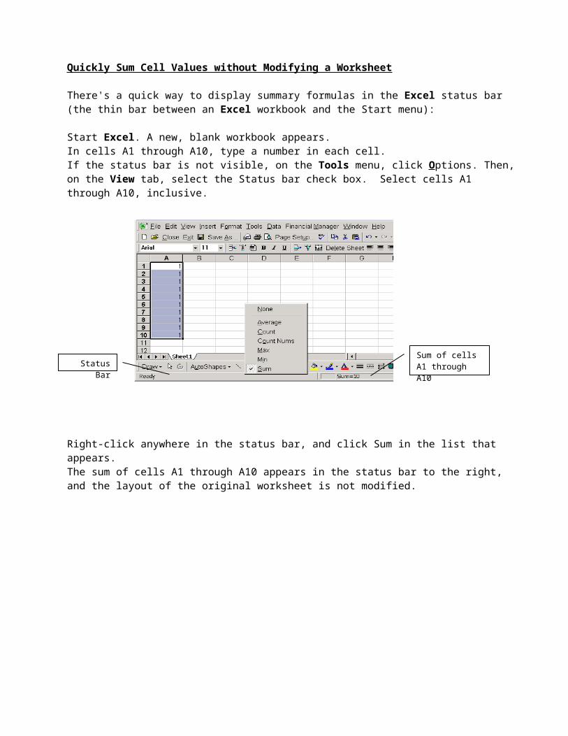
Quickly Sum Cell Values without Modifying a Worksheet
There's a quick way to display summary formulas in the Excel status bar (the thin bar between an Excel workbook and the Start menu):
Start Excel. A new, blank workbook appears. In cells A1 through A10, type a number in each cell. If the status bar is not visible, on the Tools menu, click Options. Then, on the View tab, select the Status bar check box. Select cells A1 through A10, inclusive.
Right-click anywhere in the status bar, and click Sum in the list that appears. The sum of cells A1 through A10 appears in the status bar to the right, and the layout of the original worksheet is not modified.
Status BarSum of cells A1 through A10

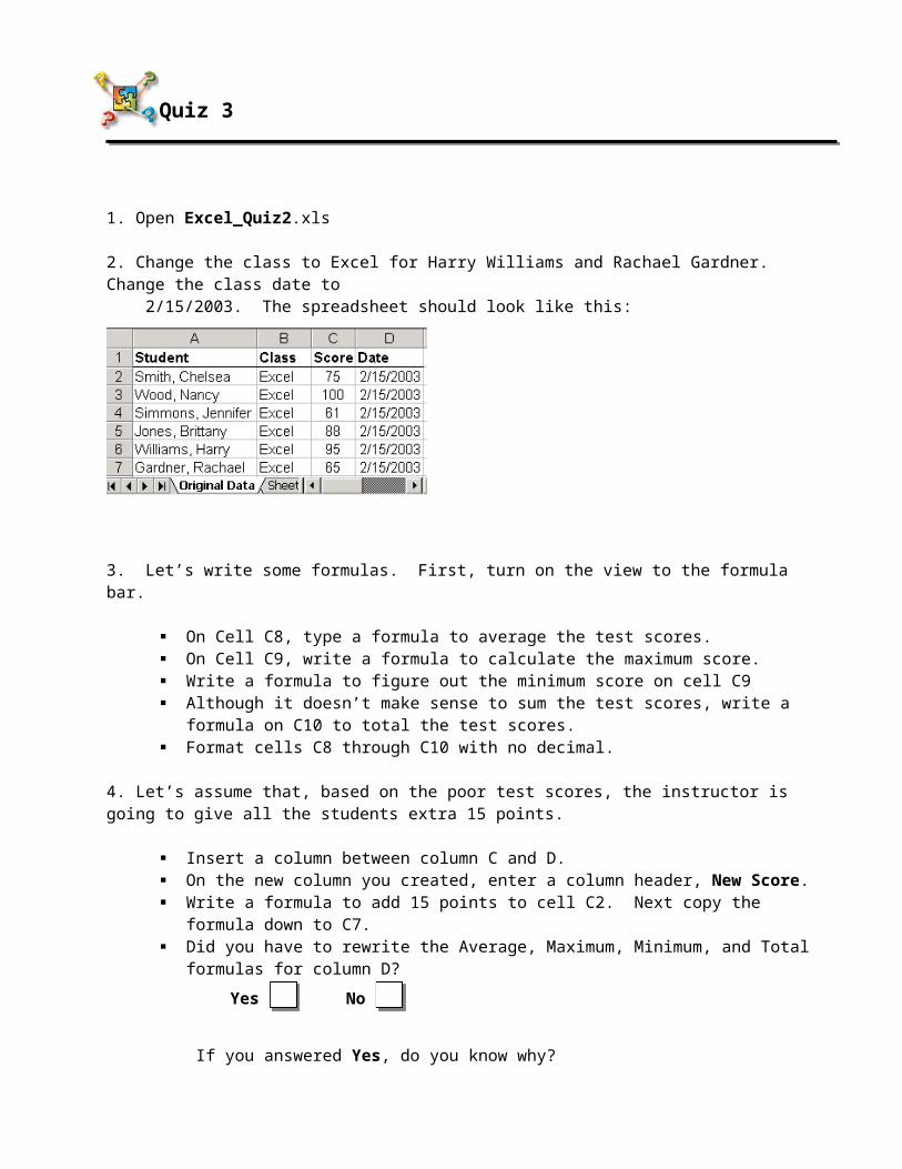
Quiz 3
1. Open Excel_Quiz2.xls
2. Change the class to Excel for Harry Williams and Rachael Gardner. Change the class date to 2/15/2003. The spreadsheet should look like this:
3. Let’s write some formulas. First, turn on the view to the formula bar.
On Cell C8, type a formula to average the test scores. On Cell C9, write a formula to calculate the maximum score. Write a formula to figure out the minimum score on cell C9 Although it doesn’t make sense to sum the test scores, write a formula on C10 to total
the test scores. Format cells C8 through C10 with no decimal.
4. Let’s assume that, based on the poor test scores, the instructor is going to give all the students extra 15 points.
Insert a column between column C and D. On the new column you created, enter a column header, New Score. Write a formula to add 15 points to cell C2. Next copy the formula down to C7. Did you have to rewrite the Average, Maximum, Minimum, and Total formulas for column
D?
If you answered Yes, do you know why?
4. Save the file as Formula_Quiz3.xls
Yes No

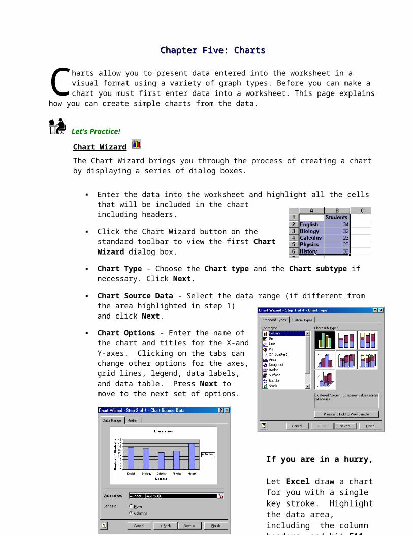
Chapter Five: ChartsChapter Five: Charts
harts allow you to present data entered into the worksheet in a visual format using a variety of graph types. Before you can make a chart you must first enter data into a worksheet. This page explains how you can create simple charts from the data. C
Let’s Practice!
Chart Wizard The Chart Wizard brings you through the process of creating a chart by displaying a series of dialog boxes.
Enter the data into the worksheet and highlight all the cells that will be included in the chart including headers.
Click the Chart Wizard button on the standard toolbar to view the first Chart Wizard dialog box.
Chart Type - Choose the Chart type and the Chart subtype if necessary. Click Next.
Chart Source Data - Select the data range (if different from the area highlighted in step 1) and click Next.
Chart Options - Enter the name of the chart and titles for the X-and Y-axes. Clicking on the tabs can change other options for the axes, grid lines, legend, data labels, and data table. Press Next to move to the next set of options.
If you are in a hurry,
Let Excel draw a chart for you with a single key stroke. Highlight the data area, including the column headers, and hit F11.

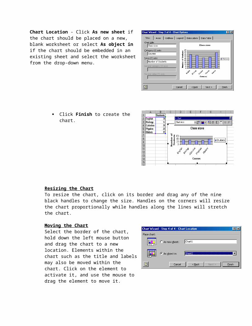
Chart Location - Click As new sheet if the chart should be placed on a new, blank worksheet or select As object in if the chart should be embedded in an existing sheet and select the worksheet from the drop-down menu.
Click Finish to create the chart.
Resizing the ChartTo resize the chart, click on its border and drag any of the nine black handles to change the size. Handles on the corners will resize the chart proportionally while handles along the lines will stretch the chart.
Moving the ChartSelect the border of the chart, hold down the left mouse button and drag the chart to a new location. Elements within the chart such as the title and labels may also be moved within the chart. Click on the element to activate it, and use the mouse to drag the element to move it.
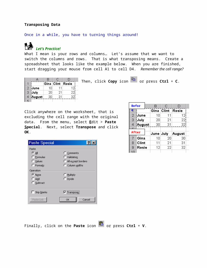
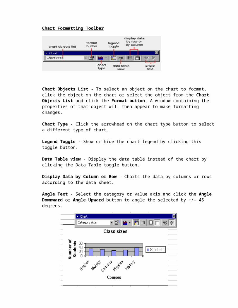
Chart Formatting Toolbar
Chart Objects List - To select an object on the chart to format, click the object on the chart or select the object from the Chart Objects List and click the Format button. A window containing the properties of that object will then appear to make formatting changes.
Chart Type - Click the arrowhead on the chart type button to select a different type of chart.
Legend Toggle - Show or hide the chart legend by clicking this toggle button.
Data Table view - Display the data table instead of the chart by clicking the Data Table toggle button.
Display Data by Column or Row - Charts the data by columns or rows according to the data sheet.
Angle Text - Select the category or value axis and click the Angle Downward or Angle Upward button to angle the selected by +/- 45 degrees.
Copying the Chart to Microsoft Word
A finished chart can be copied into a Microsoft Word document. Select the chart and click Copy or Ctrl + C. Open the destination document in Word and click Paste or Ctrl + V.

Quiz 4
1. Start Excel and create a new spreadsheet using the following example.
2. Create a bar graph. Use following titles
Chart Title: StudentsX-Axis: CoursesY-Axis: Number of Students
Insert the chart as the object in the sheet 1.
3. Change the font size for the X and Y axis labels to Arial 10.
4. Resize the chart and make it bigger. Change the color of the bars to Blue.
5. Save the Chart as Charts.xls in C:\EXCEL Training folder.
6. Open Charts.xls. On cell C1, enter a column header, Grade: A. Starting from cell C2, enter the following data:
7. Modify the existing chart to include column C.
Chapter Six: Saving Your WorkWhen you save a file for the first time, Save As option box will be activated. Select the folder to save the file to by clicking on the Save in: box. For training purposes, we will save this file in C:\EXCEL Training. When you are ready, type the name of the file then click Save.If you are not saving for the first time, you can click on the Save icon from the toolbar. Or you can enter Ctrl and S from the keyboard. All Excel files are saved with an extension ‘xls’ by default.
Just a little friendly reminder! Make sure you save your work often. If you are working with a huge document, it is crucial that you do so. Many users have shed warm salty tears after losing hours, if not days, of hard work!

Guidelines for Naming WorkbooksGuidelines for Naming Workbooks
To make it easier to find your workbooks, you can use long, descriptive file names. The complete path to the file, including drive letter, server name, folder path, file name, and a three-character file name extension, can contain up to 218 characters. File names cannot include any of the following characters: /, \, >, <, *, ?, ", |, :, or;.
Next, find the file we just saved and open it again. As usual there are several ways to open a file:
Start Excel. Click on the File menu. This menu lists most recently opened files. You can click on our file name from here.
Start Excel. From the File menu, click on Open or click on the Open icon from the tool bar.
Or from the Windows Explorer, click on the directory, folder, and the file name.
The Importance of Planning Your WorkbookThe Importance of Planning Your Workbook In reality, your spreadsheet will be much bigger than our examples. Some workbooks have thousands of records in multiple worksheets. In addition some of the cells may be linked. It is worthwhile to think in advance about the type of data you will gather and maintain.
Will you be the only user of the spreadsheet or are you going to share it with other? If so, do you need to protect the data and the workbook with a password?
How will you sort the data? If you enter the first name first, the name sort will be based on the first name. When you have four records, it is not hard to reenter them. However, it is a different senario when you have hundreds or thousands of records.
Will you be using the same file to produce address labels or form letters? Going back to our example, let’s assume that you sorted the spreadsheet by name.
The names have been entered with the first name first. So the sort will be by first name. Typically this is not very useful. It won’t be hard to change our sample and reenter the names to display lastnames first followed by a comma and the first name. However, would you like to do that with 200, 500, or 1000 names? There is always an exception. If you intend to use the same list to mail merge with a form letter, you may want to consider separating the first name and the last name into two separate columns; one for last name and the other for first name.
Now it’s getting a little tricky, right? Not really. A bit of advance planning will save you so much time and frustration later.
Here is the modified spreadsheet sorted in name order.
Prepare a Workbook to PrintPrepare a Workbook to Print
Print Preview Select File > Print Preview from the menu bar to view how the worksheet will print. Click the Next and Previous buttons at the top of the window to display the pages and click the Zoom button to view the pages closer. Make page layout modifications needed by clicking the Page Setup button. Click Close to return to the worksheet or Print to continue printing.
Print To print the worksheet, select File>Print from the menu bar.
Print Range Select either all pages or a range of pages to print.
Print What Select cells highlighted on the worksheet, the active worksheet, or all the worksheets in the entire workbook.
Copies Choose the number of copies that should be printed. Check the Collate box if the pages should remain in order.
Page SetupSelect File > Page Setup from the menu bar to format the page, set margins, and add headers and footers.
Page Select the Orientation under the Page tab in the Page Setup window to make the page Landscape or Portrait. The default setting is Portrait. The size of the worksheet on the page can also be formatted under Scaling. To force a worksheet to print only one page wide so all the columns appear on the same page, select Fit to 1 Page(s) wide.
Margins Change the top, bottom, left, and right margins under the Margins tab. Enter values in the header and footer fields to indicate how far from the edge of the page this text should appear. Check the boxes for centering horizontally or vertically on the page.
Header/FooterAdd preset headers and footers to the page by clicking the drop-down menus under the Header/Footer tab.
Enter number of copies to print
Print the entire spreadsheeet

To modify a preset header or footer, or to make your own, click the Custom Header and Custom Footer buttons. A new window will open allowing you to enter text in the left, center or right on the page.
Format text – Click this button after highlighting the text to change the font, size, and style.Page Number – Insert the page number of each page.Total Number of Pages – Use this feature along with this page number to create strings such as “page 1 of 15.”
Date – Add the date to print
Time – Add the time to print
File Name – Add the name of the workbook file
Worksheet Name – Add the name of the worksheet
Sheet Check Gridlines if you want the gridlines dividing the cells to be printed on the page. If the worksheet is several pages long and only first page includes titles for the columns, select Rows to repeat at top to choose a title row that will be printed at the top of each page.
Page BreaksTo set page breaks within the worksheet, select the row you want to appear just below the page break by clicking the row’s label. Then choose Insert > Page Break from the menu bar. You may need to click the double down arrow at the bottom of the menu list to view this option.
format text
page number date
total number of pages
time
File name
worksheet name
Shortcuts You Will Use Over and Over
The good news is that many of the shortcuts, function keys, and icons are applicable in many of the Microsoft Office Suite Software packages. To find out more, go the Microsoft Excel Keyboard Shortcuts in the Appendix section of this manual.
If you are interested in finding out more, type “Keyboard shortcuts” using the Office Assistant.
F4 to Repeat the last keyboard action
Undo and Redo icons are your friends
Ctrl and C to Copy
Ctrl and O to Open a workbook
Ctrl and V to Paste
Ctrl and S to Save a file
F7 to Spellcheck
When You Need HelpWhen You Need HelpWhen you have questions, you can click on the Office Assistant. Type in the question of your choice and click Search. In this example, search subject is “saving a spreadsheet.”
Clicking on Save a workbook results in following information.
You can also use the F1 key to activate the help option.
Click on this icon to look at the complete list of help topics.
Click on the topic of your choice.
Click here to print.
Use the arrows to go back and forth between screens.
Congratulations!
AppendixAppendix
Microsoft Excel Keyboard Shortcuts
Action KeystrokeDocument Actions
Open a file CTRL+O
New file CTRL+NSave As F12
Save CTRL+S
Print CTRL+PFind CTRL+FReplace CTRL+HGo to F5
Cursor MovementOne cell up up arrowOne cell down down arrowOne cell right TabOne cell left SHIFT+TabTop of worksheet (cell A1) CTRL+HomeEnd of worksheet (last cell with data) CTRL+EndEnd of row HomeEnd of column CTRL+left arrowMove to next worksheet CTRL+PageDown
FormulasApply AutoSum ALT+=Current date CTRL+;Current time CTRL+:
Action KeystrokeSelecting Cells
All cells left of current cell SHIFT+left arrowAll cells right of current cell SHIFT+right arrowEntire column CTRL+SpacebarEntire row SHIFT+SpacebarEntire worksheet CTRL+A
Text Style
Bold CTRL+BItalics CTRL+I
Underline CTRL+UStrikethrough CTRL+5
FormattingEdit active cell F2Format as currency with 2 decimal places SHIFT+CTRL+$Format as percent with no decimal places SHIFT+CTRL+%
Cut CTRL+X
Copy CTRL+C
Paste CTRL+V
Undo CTRL+Z
Redo CTRL+YFormat cells dialog box CTRL+1Macros ALT+F8
Help F1Spelling F7
Note: A plus sign indicates that the keys need to be pressed at the same time.
48 Introduction to Microsoft Excel
Introduction to Microsoft Excel 49
Password Protect Cells, Worksheets, and FilesPassword Protect Cells, Worksheets, and Files
If you share a spreadsheet with other users, you can protect the data by saving it with a password.
To password protect a file, File > Save As.
Next click on Tools > General Options. Type a password in the box next to “Password to open.” To allow access to your file as a reader only, click on “Password to modify” only.
Retype the password to confirm it.
The next time you open this file, you will be prompted for a password.
To password protect a worksheet without protecting the file, you can lock cells, rows, and/or columns. Highlight the cells you want to lock.
Then click on Format > Cells and select the Protection tab. Make sure the Locked option is check marked.
Next click on Tools > Protect Sheet. Make your selection whether you want to protect the Sheet, Workbook, or Protect and share a Workbook. To protect it with a password, enter a password.
To unlock cells, unprotect the worksheet first.
50 Introduction to Microsoft Excel

Customizing the Toolbar
When you first start Excel, two toolbars – the Standard and Formatting toolbars- appear by default. As you work with Excel, you may want to display other toolbars, such as the Drawing toolbar or the Chart toolbar. The figure below displays that the standard, formatting and drawing toolbars are currently active.
To add another Toolbar
From the menu, select View > Toolbars (or Tools > Customize.) Click any of the toolbar option that has not been selected already. Click on it once to select it and again to deselect it. It is a toggle option.
To customize your existing toolbar
From the menu, select View > Toolbars > Customize (or Tools > Customize.) Then click on the Commands tab. This window is organized by Categories and their associated commands. For instance, the File Category has New, Open, Close, Save, Save As…. Commands. To view more, click on the vertical scroll bar. You can literally drag and drop selected command to the existing tool bar. You may ask, why would I want to do that? As you venture further into the Excel world, you might find yourself exhausted from going to the menu for the hundredth time to use the Page Setup from the File menu. You never get tired like that? O.K. But you will soon see how convenient it is to have the Page Setup icon on the toolbar.
Introduction to Microsoft Excel 51
Scroll down and find the Page Setup command.
Click on it with the left mouse button. Hold it down and start dragging it up to the Standard tool bar.
Hint: The reverse is true when you want to remove any icons from the toolbars. You must activate the Customize menu first. Then click on the icon you want to remove. Hold it down and start dragging it down to the Customize window. Once the icon is anywhere in the Customize window, you can release the left mouse button.
This is what the menu looks like after Page Setup command has been added. You can drag and drop a command anywhere on the toolbar. In this example, it was placed next to the Print Preview icon.
52 Introduction to Microsoft Excel
53
As soon as you right-mouse click on the command to add to the toolbar, the cursor changes like this.
Searching for Help on the Web
The Internet offers wealth of information. You can type a search subject in the search box and get dozens of hits on a selected subject.
http://www.microsoft.com/office/Excel/
This site is the top pick and no wonder. It is the official Microsoft Office Site. Type Excel 2000 in the Search This Site box and click Go…
54 Introduction to Microsoft Excel
There are many more but here are just some of the sites:
Basic Excel Tutorialhttp://www.usd.edu/trio/tut/excel/
Formulas, Formulas, and more Formulashttp://www.barasch.com/excel/xlformulas.htm#desposition%20of%20the%20files
Excel User Tips, click on User Tips.http://j-walk.com/ss/excel/
This is a video tutorial. Answer “Yes” to the initial runtime error. Then select a subject to preview.http://www.exitnow.com/skillbuilder/viewlets/excel2000.htm
Introduction to Microsoft Excel 55