Excel Advanced Training

Index

Excel 2007 Training

Index Description

1. Quick Access Toolbar i Guide to setting up the quick access toolbar in Excel 2007

2. New Functions i Explanation of new worksheet function available in Excel 2007 eg. IFERROR, COUNIFS, SUMIFS

3. Formatting Techniques i Basic formatting - Text alignment, Font size and style, Word wrapping

ii Format Cells dialogue

iii Merge and Unmerged cells

iv Conditional Formatting

vi Data validation combined with conditional formatting Advanced Topic

4. Page and Print Setup i Page break view and page setup

ii Setting the page "header" and "footer"

5. Short Cut Keys i Most useful Excel keyboard shortcuts

ii Select and move charts

6. IF Statement i Comparison Operators

ii Multiple tests using nested if statements

iii Advanced tests using logical operators

7. Lookup Function i VLOOKUP exact match, nearest match, common mistakes and problems faced by consultants

ii Advanced lookup functions using INDEX, MATCH and OFFSET

8. Autofilter i Common difficulties

9. Goal Seek dialogue i Using Goal Seek to search for the solution

10. Named Ranges i Naming cells and using names to simplify calculations

ii Dynamic Ranges Advanced Topic

11. Go To dialogue i Using the GoTo dialogue to efficiently navigate workbooks

ii. Use the GoTo Special for advanced navigation including: selecting and deleting blank rows Advanced Topic

12. Pivot Tables i The difference between Excel 2007 Pivot tables and classic style Pivot tables (Not yet available)

ii Setting up a pivot table in 2007 and understanding the options available (Not yet available)

iii Advanced pivot table functionality (Not yet available )

13. Charting Not yet available

14. Find & Replace dialogue i Find and Replace options and functionality

ii Use find a replace to modify formatting

iii Use find and replace to modify formulas and references to other workbooks Advanced Topic

15. Array Formulas i What are array formulas

ii Transpose and frequency formulas

iii Advanced queries and calculations using array formulas Advanced Topic

16. Iterative and cyclic calculations Not yet available Advanced Topic

Appendix A. Functions list i. List and description of frequently used Excel functions including examples

ii. Using "Text functions" to cure capitalisation disease

Working draft V1 07/08/2008

Excel 2007 Training

The quick access toolbar is a customisable toolbar found above the menus called ribbons

1. Select the "Office button" at the top right hand side of the Excel window

2. Select "Excel Options" at the bottom of the Office button menu

3. Within options select the "Customize" tab

5. Click Add

6. If you would like to remove a command, select it from your list and click "Remove"

Steps to setting adding your favorite commands to the quick access

toolbar

Investing time in setting up your Excel 2007 quick access toolbar can significantly reduce

frustration and improve productivity when first making the switch from older versions

4. Select your favorite commands from the list on the left. To help find your

favorite commands you can sort by the various command categories from the

pull down menu

- "Popular Commands"

- "Commands Not in the ribbon"

- "All Commands"

- Commands found in the "Home Tab"

etc.

The new "Office Button" replaces the file menu

The quick access customisable toolbar

Excel 2007 menus, also called ribbons

1. QuickAccessToolbar 2/30

Excel 2007 Training

You may wish to shift the quick access toolbar below the ribbon.

6. Check the "Show Quick Access Toolbar below the Ribbon" box in options

or

You may wish to minimise the ribbon so that it only appears when you have your mouse pointer near it

Using the same options menu, select "Minimize the Ribbon"

At the end of the quick access toolbar you will find a menu button shaped as a downward facing arrow. When selected you will find a

set of options. Select "Show Above/Below the Ribbon"

Quick access options menu is found on the right hand side of the toolbar

1. QuickAccessToolbar 3/30

Excel 2007 Training

Syntax : IFERROR(value,value_if_error)

Example: How do I prevent Excel returning an error whenever VLOOKUP can not find the search string

Excel 2003 Solution

=IF(ISERROR(VLOOKUP("Josh", LookupTable, 3, FALSE)), " Value not found", VLOOKUP("Josh", LookupTable, 3, FALSE))

Excel 2007 Solution

=IFERROR(VLOOKUP("Clare”, LookupTable, 3, false), “Value not found”)

Syntax: AVERAGEIF(Range, Criteria, [Average Range])

Excel 2003 Solution - Array formula solution (see section "15. Array formulas")

{=AVERAGE(IF(D45:D49="Coke",E45:E49,""))} 2

Excel 2007 Solution

=AVERAGEIF(D45:D49,"Coke",E45:E49) 2

The "...IFS" functions provide simple solutions to the problems of summing, counting and averaging with multiple criteria.

Syntax: SUMIFS(sum_range, criteria_range1, criteria1 [,criteria_range2, criteria2…])

COUNTIFS(criteria_range1, criteria1 [,criteria_range2, criteria2…])

AVERAGEIFS(average_range, criteria_range1, criteria1 [,criteria_range2, criteria2…])

Example: if a user had the following Database, how could they sum “Units” where Beverage = “Coke” and Name = “Josh”

Database

Name Beverage Units

Josh Sprite 2

Josh Coke 2

Julia Coke 3

Josh Coke 1

Prue Sprite 1

Excel 2003 Solution - Array formula solution (see section "15. Array formulas")

{=SUM(IF(C2:C17="Apple", IF(D2:D17="One", B2:B17, 0), 0))} 3

The formula is hard to set up correctly, many users do not know about array formulas, and it is harder to read/debug.

Excel 2007 Solution

=SUMIFS(E44:E48,C44:C48,"Josh",D44:D48,"Coke") 3

The formula is much simpler to write, easier to read, and doesn’t require array entry.

COUNTIFS and AVERAGEIFS, also new to Excel 2007, work the same way with the same benefits.

Excel 2007 has added five new and very useful functions to the Excel function library

AVERAGEIF provides a single function to conditionally average a range of numbers based on a specific criteria – a complement to SUMIF and COUNTIF.

IFERROR simplifies error checking by providing a simple method to catch errors - an extension of ISERROR.

Example: returns the average of "Units" where the corresponding value in "Column Beverage" is equal to "Coke"

New Function 3,4,5: SUMIFS / COUNTIFS / AVERAGEIFS

New Function 1: IFERROR

New Function 2: AVERAGEIF

2. New Functions 4/30

Excel 2007 Training

Excel offers many formatting options for the contents of cells

Most formatting option can be accessed from the "Home" RibbonHome -> Font Group & Alignment Group & Number Group

The most regularly used options should be included in the quick access toolbar

Text Alignment Toggle Gridlines

View -> Show/ Hide Group -> Gridlines

Bold, Italic and Underline

Note Keyboard shortcuts are useful: Ctrl + B, Ctrl + I, Ctrl + U

Font Style and Size

Borders

Wrap Text Row and Column height and width

3. Formatting 5/30

Excel 2007 Training

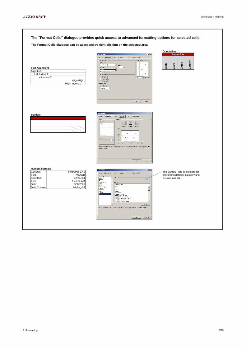
The "Format Cells" dialogue provides quick access to advanced formatting options for selected cells

The Format Cells dialogue can be accessed by right-clicking on the selected area

Orientation

Text Alignment Jo

sh

Cla

re

Ch

loe

Caro

lyn

Borders

Number Formats

Right Indent 1:

Align Left:

Left Indent 1:

Left Indent 2:

Super BAs

Align Right:

=NOW()

3.97E+04

The Sample Field is excellent for

previewing different category and

custom formats

General:

Text:

Scientific:

Time:

Date:

Date Custom:

1:41:34 AM

8/08/2008

08-Aug-08

8/08/2008 1:41

3. Formatting 6/30

Excel 2007 Training

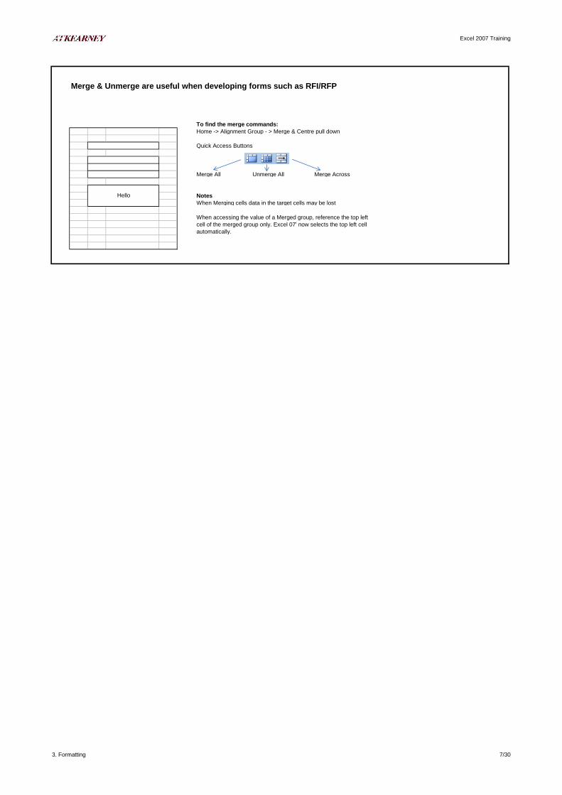
Merge & Unmerge are useful when developing forms such as RFI/RFP

To find the merge commands:

Home -> Alignment Group - > Merge & Centre pull down

Quick Access Buttons

Merge All Unmerge All Merge Across

Notes

When Merging cells data in the target cells may be lost

When accessing the value of a Merged group, reference the top left

cell of the merged group only. Excel 07' now selects the top left cell

automatically.

Hello

3. Formatting 7/30

Excel 2007 Training

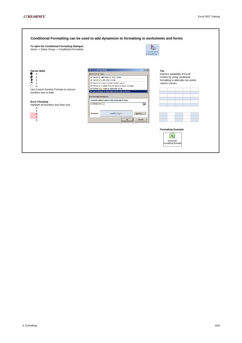
Conditional Formatting can be used to add dynamism to formatting in worksheets and forms

To open the Conditional Formatting dialogue:

Home -> Styles Group -> Conditional Formatting

Harvey Balls Tip:

4

3

2

1

0

Error Checking

Highlight All Numbers less than zero

4

3

-2

-1

0

Formatting Example

Improve readability of Excel

models by using conditional

formatting to alternate row and/or

column colours

Use Custom Number Formats to remove

numbers next to balls

Advanced Formatting Example

3. Formatting 8/30

Excel 2007 Training

Data Validation can be used to prohibit invalid inputs to forms and prompt correct inputs

To open the Data Validation dialogue

Data - > Data Tools Group -> Data Validation

Example 1

Data validation with prohibitive error alert

Example 2

Data validation with warning only

Example 3

Data validation with conditional formatting

Is your company a distributor?

(Yes/No)No

How many manufacturers does

your company represent as a fully

authorized distributor?

3. Formatting 9/30

Excel 2007 Training

The easiest way to format a spreadsheet for print is to use the page break

To go to Page Break View: View -> Page Break

To return to Normal View: View -> Normal

Example

Set the print range

1. Drag and place the blue lines to set the print range

2. Insert Page breaks by right clicking on the desired column number and selecting insert page break

Set the page setup and Header/Footer

3. Open the Page Setup dialogue (In page break view Right Click -> Page Setup, or in Print Preview select Page Setup in top left hand corner)

4. Set the page orientation and adjust the page scale

Set the Header/Footer

5: Set the page count using the page numbers option

All Spreadsheet to be handed to clients or sent to suppliers should be formatted for printing like any

deliverable

Note: On Selecting Fit to - Excel will ignore defined page breaks and automatically set the page breaks as to best fit the number of pages. This

may be an undesired outcome if tables should not be split between pages. Instead manually set the Adjust to scale

Print Setup Example

4. Page Setup 10/30

Excel 2007 Training

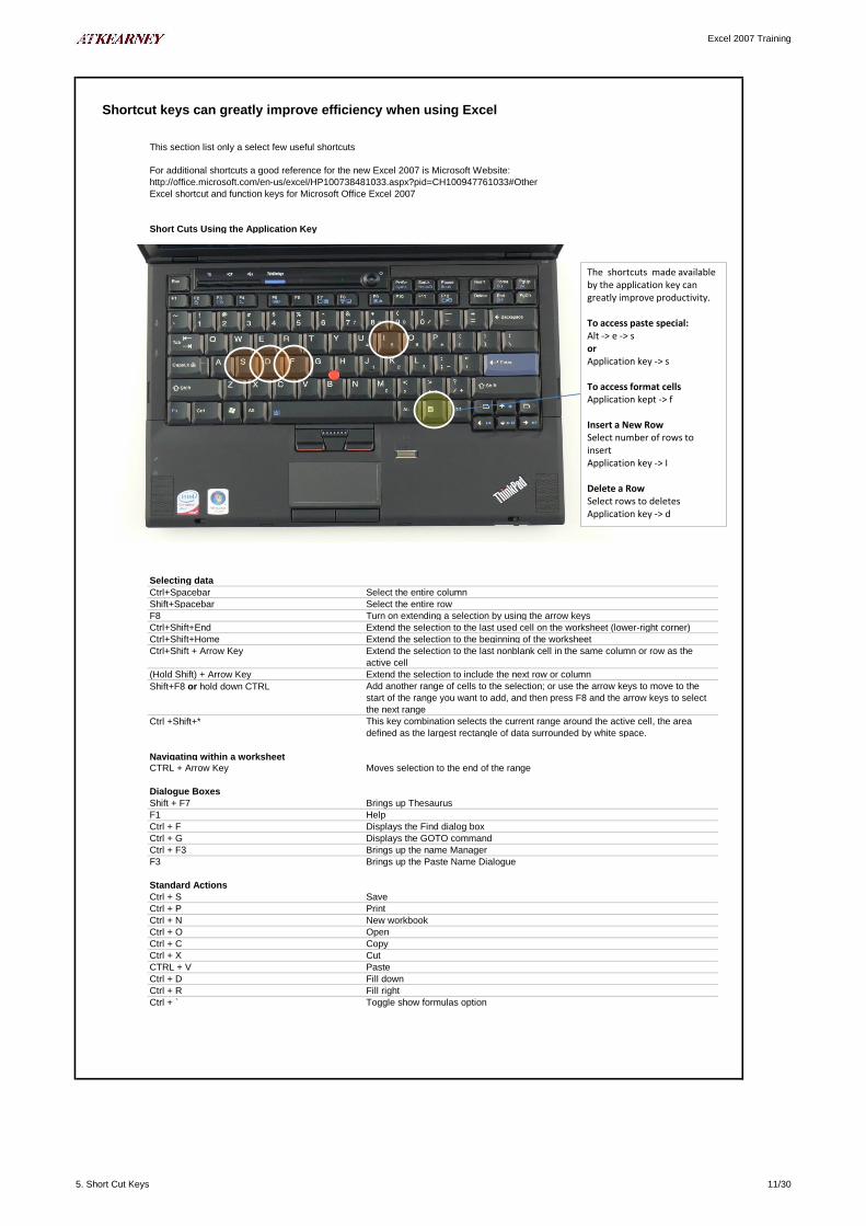
Shortcut keys can greatly improve efficiency when using Excel

http://office.microsoft.com/en-us/excel/HP100738481033.aspx?pid=CH100947761033#Other

Excel shortcut and function keys for Microsoft Office Excel 2007

Short Cuts Using the Application Key

Selecting data

Ctrl+Spacebar Select the entire column

Shift+Spacebar Select the entire row

F8 Turn on extending a selection by using the arrow keys

Ctrl+Shift+End Extend the selection to the last used cell on the worksheet (lower-right corner)

Ctrl+Shift+Home Extend the selection to the beginning of the worksheet

Ctrl+Shift + Arrow Key Extend the selection to the last nonblank cell in the same column or row as the

active cell

(Hold Shift) + Arrow Key Extend the selection to include the next row or column

Shift+F8 or hold down CTRL Add another range of cells to the selection; or use the arrow keys to move to the

start of the range you want to add, and then press F8 and the arrow keys to select

the next range

Ctrl +Shift+* This key combination selects the current range around the active cell, the area

defined as the largest rectangle of data surrounded by white space.

Navigating within a worksheet

CTRL + Arrow Key Moves selection to the end of the range

Dialogue Boxes

Shift + F7 Brings up Thesaurus

F1 Help

Ctrl + F Displays the Find dialog box

Ctrl + G Displays the GOTO command

Ctrl + F3 Brings up the name Manager

F3 Brings up the Paste Name Dialogue

Standard Actions

Ctrl + S Save

Ctrl + P Print

Ctrl + N New workbook

Ctrl + O Open

Ctrl + C Copy

Ctrl + X Cut

CTRL + V Paste

Ctrl + D Fill down

Ctrl + R Fill right

Ctrl + ` Toggle show formulas option

This section list only a select few useful shortcuts

For additional shortcuts a good reference for the new Excel 2007 is Microsoft Website:

The shortcuts made available by the application key can greatly improve productivity.

To access paste special:Alt -> e -> sorApplication key -> s

To access format cellsApplication kept -> f

Insert a New RowSelect number of rows to insertApplication key -> I

Delete a RowSelect rows to deletesApplication key -> d

5. Short Cut Keys 11/30

http://office.microsoft.com/en-us/excel/HP100738481033.aspx?pid=CH100947761033

Excel 2007 Training

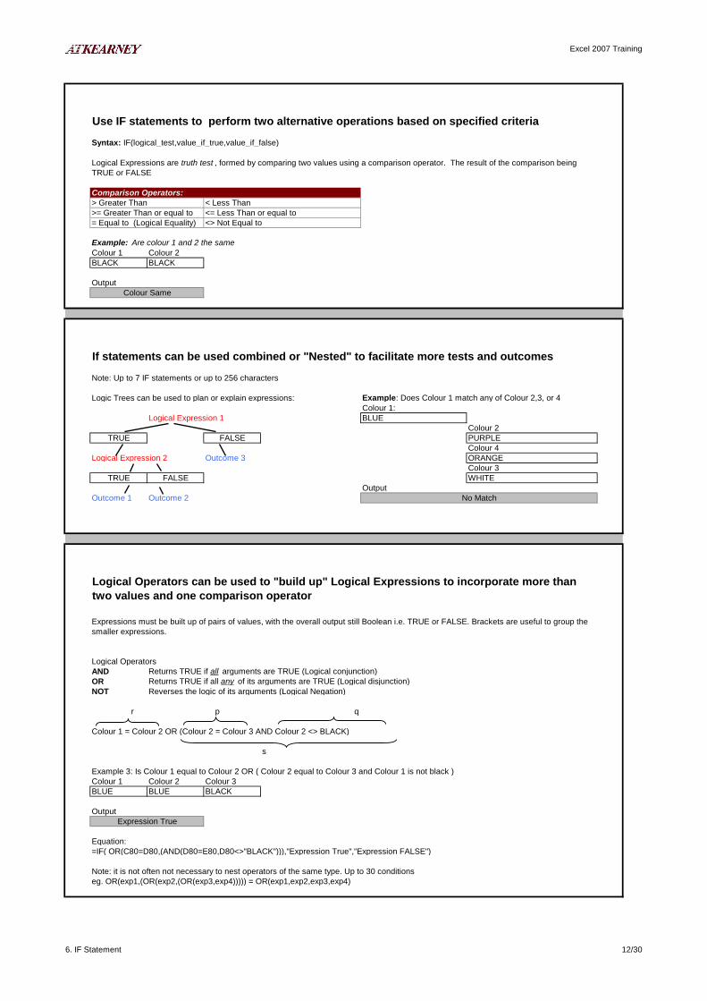
Use IF statements to perform two alternative operations based on specified criteria

Syntax: IF(logical_test,value_if_true,value_if_false)

Comparison Operators:

Example: Are colour 1 and 2 the same

Colour 1 Colour 2

BLACK BLACK

Output

If statements can be used combined or "Nested" to facilitate more tests and outcomes

Note: Up to 7 IF statements or up to 256 characters

Logic Trees can be used to plan or explain expressions: Example: Does Colour 1 match any of Colour 2,3, or 4

Colour 1:

Logical Expression 1 BLUE

Colour 2

TRUE FALSE PURPLE

Colour 4

Logical Expression 2 Outcome 3 ORANGE

Colour 3

TRUE FALSE WHITE

Output

Outcome 1 Outcome 2

Logical Operators

AND Returns TRUE if all arguments are TRUE (Logical conjunction)

OR Returns TRUE if all any of its arguments are TRUE (Logical disjunction)

NOT Reverses the logic of its arguments (Logical Negation)

r p q

Colour 1 = Colour 2 OR (Colour 2 = Colour 3 AND Colour 2 <> BLACK)

s

Example 3: Is Colour 1 equal to Colour 2 OR ( Colour 2 equal to Colour 3 and Colour 1 is not black )

Colour 1 Colour 2 Colour 3

BLUE BLUE BLACK

Output

Equation:

=IF( OR(C80=D80,(AND(D80=E80,D80<>"BLACK"))),"Expression True","Expression FALSE")

Note: it is not often not necessary to nest operators of the same type. Up to 30 conditions

eg. OR(exp1,(OR(exp2,(OR(exp3,exp4))))) = OR(exp1,exp2,exp3,exp4)

Logical Expressions are truth test , formed by comparing two values using a comparison operator. The result of the comparison being

TRUE or FALSE

= Equal to (Logical Equality)

>= Greater Than or equal to

> Greater Than < Less Than

<= Less Than or equal to

<> Not Equal to

Expressions must be built up of pairs of values, with the overall output still Boolean i.e. TRUE or FALSE. Brackets are useful to group the

smaller expressions.

Expression True

Colour Same

No Match

Logical Operators can be used to "build up" Logical Expressions to incorporate more than

two values and one comparison operator

6. IF Statement 12/30

Excel 2007 Training

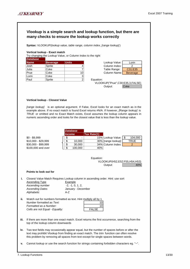
Syntax: VLOOKUP(lookup value, table range, column index, [range lookup] )

Vertical lookup - Exact match

Try changing the Lookup Value, or Column Index to the right

Database

Name Beverage Units Lookup Value: Lorin

Josh Sprite 4 Column Index: 2

Julia Coke 7 Table Range: C31:E35

Prue Coke 10 Column Name: Beverage

Lorin Coke 3

Paul Sprite 2 Equation:

Output: Coke

Vertical lookup - Closest Value

Database

Income Tax Rate(1)

$0 - $9,999 -$ 15% Lookup Value: 104,000$

$10,000 - $29,999 10,000$ 30% [range lookup] TRUE

$30,000 - $99,999 30,000$ 34% Column Index: 2

$100,000 and over 100,000$ 40%

Equation:

Output: 40%

Points to look out for

i. Closest Value Match Requires Lookup column in ascending order. Hint: use sort

Ascending Type Example

Ascending number -2, -1, 0, 1, 2,

Ascending Dates January - December

Alphabetic A-Z

ii. Watch out for numbers formatted as text. Hint multiply all by 1

Number formatted as Text: 10

Formatted as a Number: 10

Cells are not Equal - Equality: FALSE

iii.

iv.

v. Cannot lookup or use the search function for strings containing forbidden characters eg. "~".

Two text fields may occasionally appear equal, but the number of spaces before or after the

text may prohibit Vlookup from finding an exact match. The trim function can often resolve

this problem by removing all spaces from text except for single spaces between words.

Vlookup is a simple search and lookup function, but there are

many checks to ensure the lookup works correctly

If there are more than one exact match. Excel returns the first occurrence, searching from the

top of the lookup column downwards

VLOOKUP("Prue",C30:E35,3,FALSE)

[range lookup] is an optional argument. If False, Excel looks for an exact match as in the

example above. If no exact match is found Excel returns #N/A. If however, [Range lookup] is

TRUE or omitted and no Exact Match exists, Excel assumes the lookup column appears in

numeric ascending order and looks for the closest value that is less than the lookup value.

VLOOKUP(H52,E52:F55,H54,H53)

7. Lookup Functions 13/30

Excel 2007 Training

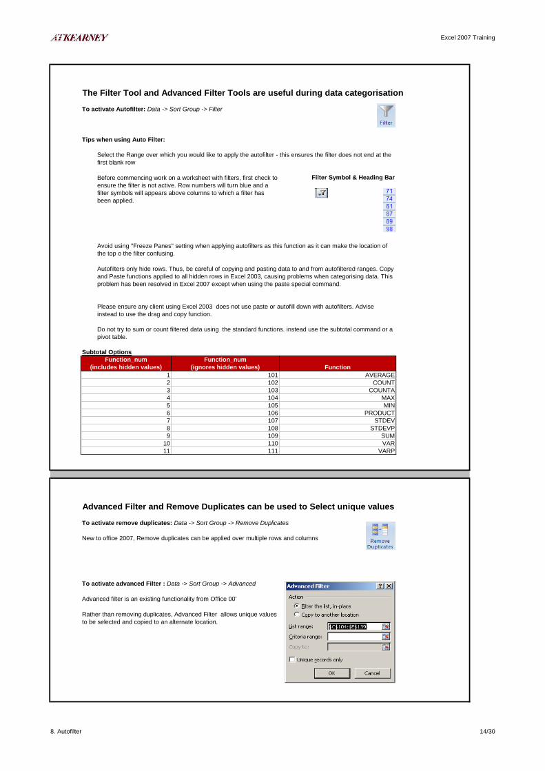
The Filter Tool and Advanced Filter Tools are useful during data categorisation

To activate Autofilter: Data -> Sort Group -> Filter

Tips when using Auto Filter:

Filter Symbol & Heading Bar

Subtotal Options

Function_num Function_num

(includes hidden values) (ignores hidden values)

1 101 AVERAGE

2 102 COUNT

3 103 COUNTA

4 104 MAX

5 105 MIN

6 106 PRODUCT

7 107 STDEV

8 108 STDEVP

9 109 SUM

10 110 VAR

11 111 VARP

Advanced Filter and Remove Duplicates can be used to Select unique values

To activate remove duplicates: Data -> Sort Group -> Remove Duplicates

New to office 2007, Remove duplicates can be applied over multiple rows and columns

To activate advanced Filter : Data -> Sort Group -> Advanced

Advanced filter is an existing functionality from Office 00'

Do not try to sum or count filtered data using the standard functions. instead use the subtotal command or a

pivot table.

Rather than removing duplicates, Advanced Filter allows unique values

to be selected and copied to an alternate location.

Function

Select the Range over which you would like to apply the autofilter - this ensures the filter does not end at the

first blank row

Before commencing work on a worksheet with filters, first check to

ensure the filter is not active. Row numbers will turn blue and a

filter symbols will appears above columns to which a filter has

been applied.

Avoid using "Freeze Panes" setting when applying autofilters as this function as it can make the location of

the top o the filter confusing.

Autofilters only hide rows. Thus, be careful of copying and pasting data to and from autofiltered ranges. Copy

and Paste functions applied to all hidden rows in Excel 2003, causing problems when categorising data. This

problem has been resolved in Excel 2007 except when using the paste special command.

Please ensure any client using Excel 2003 does not use paste or autofill down with autofilters. Advise

instead to use the drag and copy function.

8. Autofilter 14/30

Excel 2007 Training

Example Database

Subtotal 265

Sum 232

Officer Day Hours

David Mon 1

David Tue 3

David Wed 2

David Thu 3

David Fri 3

David Sat 1

David Sun 2

Phil Mon 13

Phil Tue 13

Phil Wed 13

Phil Thu 13

Phil Fri 13

Phil Sat 13

Phil Sun 13

Jeremy Mon 7

Jeremy Tue 8

Jeremy Wed 6

Jeremy Thu 3

Jeremy Fri 3

Jeremy Sat 5

Jeremy Sun 3

Peter Mon 13

Peter Tue 13

Peter Wed 13

Peter Thu 13

Peter Fri 13

Peter Sat 13

Peter Sun 13

Simon Mon 8

Simon Tue 3

Simon Wed 6

Simon Thu 3

Simon Fri 2

Simon Sat 3

Simon Sun 8

8. Autofilter 15/30

Excel 2007 Training

Goal Seek is a useful numeric equation solver

To open Goal Seek: Data -> Data Tools Group - > What-If Analysis - > Goal Seek

Solver Parameters

Set Cell The cell containing the formula that calculates the information you seek

To Value The target value - the value for which you want the set cell to equal

By Changing

Cell The input cell that Excel changes - the value you want to know

Example

What sales volume do I need to break even?

Formula

Profit = Revenue - Cost

profit ($19,500.00)

volume 10000

price $3

unit cost 0.45

fixed cost 45000

revenue $30,000.00

variable cost 4500.00

Goal Seek Options: Office Button -> Excel Options -> Formulas

Change Accuracy:

Iterations:

Limitation: if problem has more than one solution - Goal seek will only find one answer

Goal seek enables the computation of the input to a problem for which the output is known

"Maximum Change " - Goal seek will solve to an accuracy of "Maximum change" - default of 0.001

meaning accurate to -0.001 -> 0.001

"Maximum Iterations " - For difficult problems the maximum number of iterations may need increasing

to ensure convergence

Intermediary

9. GoalSeek 16/30

Excel 2007 Training

Cell names can be modified using the Name box found next to the formula bar

Names can be managed, changed and deleted using the Name manager

To open paste the Paste Name dialogue: Formulas -> Define Name Group -> Use in Formula or F3

Naming the answer to the ultimate question 42

Using the ultimate answer in a formula 84

Using hyperlinks with named ranges for navigation Click here to go to the ultimate answer

To open the Name Manager: Formulas -> Define Name Group -> Name Manage or Ctrl + F3

Use names to clarify formulas, keep track of constants or build a worksheet

index

10. Named Ranges 17/30

Excel 2007 Training

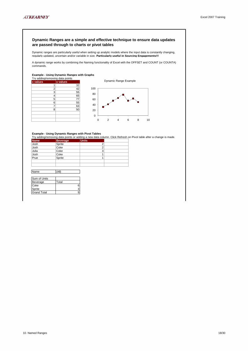
Example - Using Dynamic Ranges with Graphs

Try adding/removing data points

x values y values

1 32

2 42

3 55

4 65

5 77

6 55

7 63

8 50

Example - Using Dynamic Ranges with Pivot Tables

Try adding/removing data points or adding a new data column. Click Refresh on Pivot table after a change is made.

Name Beverage Units

Josh Sprite 2

Josh Coke 2

Julia Coke 3

Josh Coke 1

Prue Sprite 1

Name (All)

Sum of Units

Beverage Total

Coke 6

Sprite 3

Grand Total 9

Dynamic Ranges are a simple and effective technique to ensure data updates

are passed through to charts or pivot tables

Dynamic ranges are particularly useful when setting up analytic models where the input data is constantly changing,

regularly updated, uncertain and/or variable in size. Particularly useful in Sourcing Engagements!!!

A dynamic range works by combining the Naming functionality of Excel with the OFFSET and COUNT (or COUNTA)

commands.

0

20

40

60

80

100

0 2 4 6 8 10

Dynamic Range Example


Excel 2007 Training

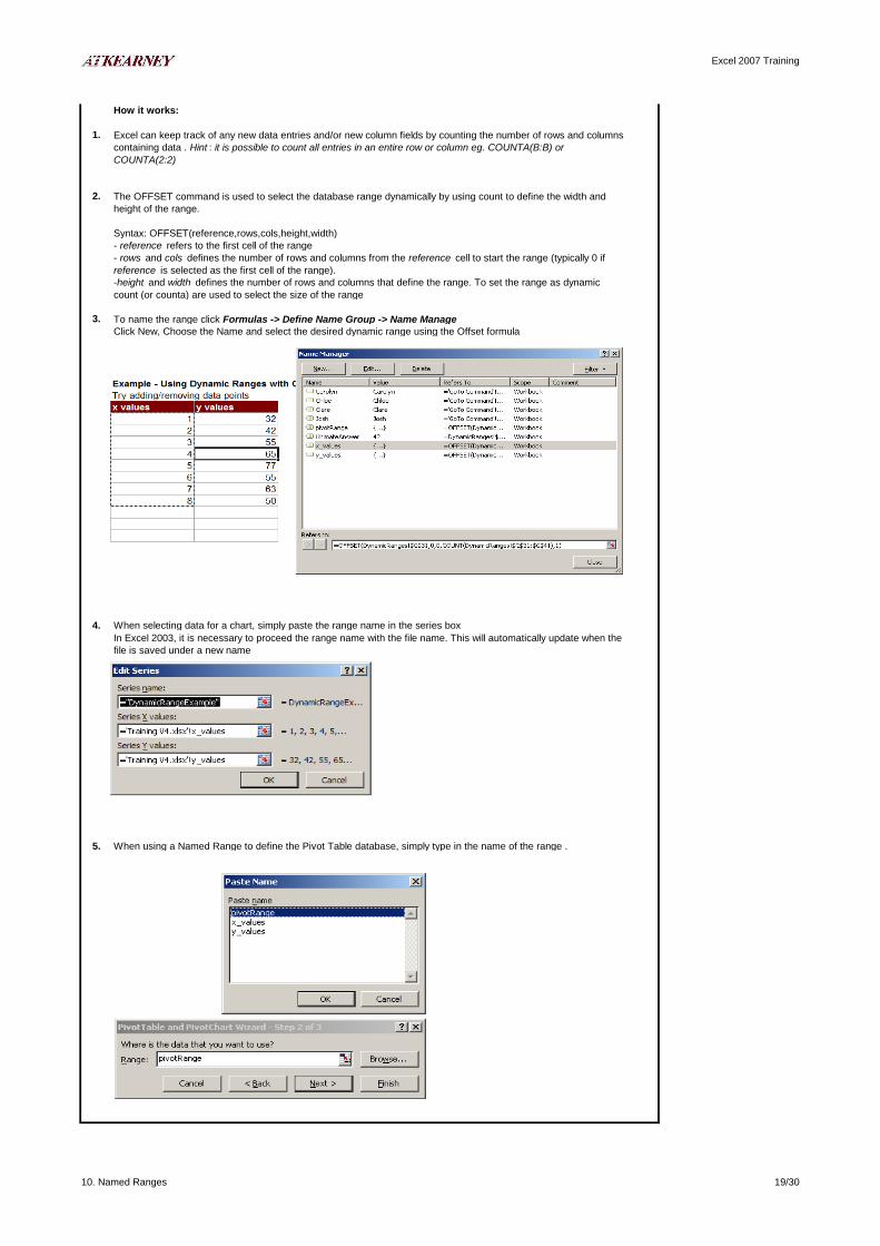
How it works:

1.

2.

3.

4. When selecting data for a chart, simply paste the range name in the series box

5. When using a Named Range to define the Pivot Table database, simply type in the name of the range .

In Excel 2003, it is necessary to proceed the range name with the file name. This will automatically update when the

file is saved under a new name

Excel can keep track of any new data entries and/or new column fields by counting the number of rows and columns

containing data . Hint : it is possible to count all entries in an entire row or column eg. COUNTA(B:B) or

COUNTA(2:2)

The OFFSET command is used to select the database range dynamically by using count to define the width and

height of the range.

-height and width defines the number of rows and columns that define the range. To set the range as dynamic

count (or counta) are used to select the size of the range

To name the range click Formulas -> Define Name Group -> Name Manage

Syntax: OFFSET(reference,rows,cols,height,width)

Click New, Choose the Name and select the desired dynamic range using the Offset formula

- reference refers to the first cell of the range

- rows and cols defines the number of rows and columns from the reference cell to start the range (typically 0 if

reference is selected as the first cell of the range).


Excel 2007 Training

Go To and Go To Special are Excel's most powerful navigation tool

To open Go To: Ctrl + g

Josh

Clare

Chloe

Carolyn

The Go To Tool will allow you to select all named cells

and ranges:

In the reference field, it is possible to type the desired cell reference or range. Try complex combinations, eg:

"K:K,N:N,10:10,15:15"

Note: References to difference worksheets are proceeded with the worksheet name and an exclamation mark as

follows: 'Worksheet Name'!A1

11. GoTo 20/30

Excel 2007 Training

Example 1: Delete blank rows

Example data - remove the blank rows in the data below

Row1 Row1 Row1

Row2 Row2 Row2

Row3 Row3 Row3

Row4 Row4 Row4

Row5 Row5 Row5

Row6 Row6 Row6

Row7 Row7 Row7

Row8 Row8 Row8

Row9 Row9 Row9

Row10 Row10 Row10

Example 2: Select precedents and/or dependent cells.

Precedents

Precedents are the inputs to a formula in the active cell

Dependents

Dependents are cells contain formulas that refer to the active cell

Use Go To Special to select the precedents to the formula in C

Formula: 1 + 2 = 3

A B C

1 2 3

Precedents to Cell C Direct Dependent to Cells A & B

Often data is provided by a client in a very rough format.

Regularly the data has missing/blank rows that must be

removed. It can be tedious to manually select and delete

these gaps. Go-To Special offers a quick and effective

approach.

Select the entire column or desired range. Use Go-To

Special to select the blank cells. Delete the blank cells

(Application key -> d). Select "Entire Row".

The Go To Special dialogue allows the quick and easy selection of objects,

comments, or cells with special characteristics or entries.

11. GoTo 21/30

Excel 2007 Training

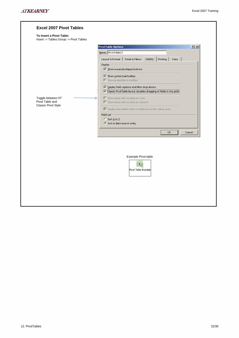
To Insert a Pivot Table:

Insert -> Tables Group -> Pivot Tables

Example Pivot table

Toggle between 07'

Pivot Table and

Classic Pivot Style

Excel 2007 Pivot Tables

Pivot Table Example

12. PivotTables 22/30

Excel 2007 Training

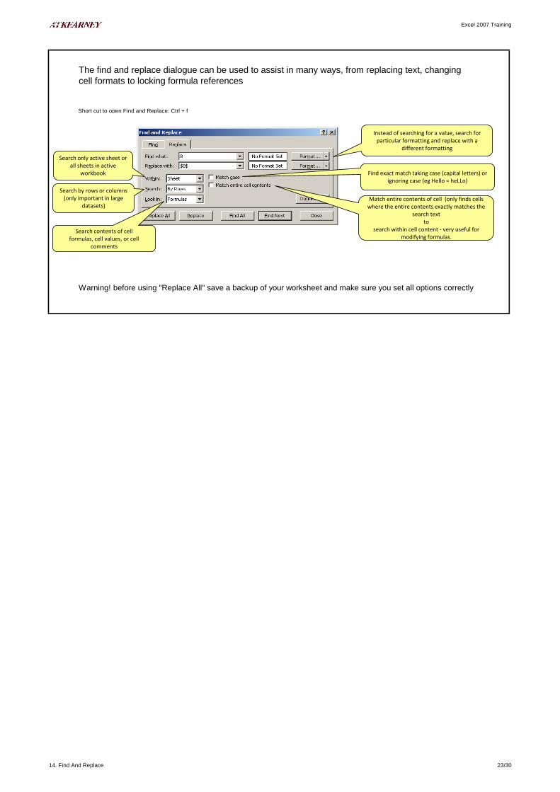
Short cut to open Find and Replace: Ctrl + f

Warning! before using "Replace All" save a backup of your worksheet and make sure you set all options correctly

The find and replace dialogue can be used to assist in many ways, from replacing text, changing

cell formats to locking formula references

Search contents of cell formulas, cell values, or cell

comments

Search only active sheet or all sheets in active

workbook

Search by rows or columns (only important in large

datasets) Match entire contents of cell (only finds cells

where the entire contents exactly matches the search text

tosearch within cell content - very useful for

modifying formulas.

Instead of searching for a value, search for particular formatting and replace with a

different formatting

Find exact match taking case (capital letters) or ignoring case (eg Hello = heLLo)

14. Find And Replace 23/30

Excel 2007 Training

Example 1 - Use Find and Replace to change formatting

10.0% 10% $0.10

20.0% 20% $0.20

30.0% 30% $0.30

40.0% 40% $0.40

50.0% 50% $0.50

Example 2 - Use Find and Replace to change a formula by locking all cells referring to column C

Column C

Resulting

Formulas

(text)

1 1 =C14 1 =$C$14

2 2 =C15 2 =$C$15

3 3 =C16 3 =$C$16

4 4 =C17 4 =$C$17

5 5 =C18 5 =$C$18

6 6 =C19 6 =$C$19

7 7 =C20 7 =$C$20

Example 3 - Use Find and Replace to change a reference to another worksheet or even workbook

It is not uncommon to link/reference data between two separate workbooks.

For example you may keep all your assumption separate in one workbook and reference your assumption in another workbook making your calculations

Unfortunately, if you change the name of your reference workbook the link is not updated.

One way to resolve this is to search for the original workbook name within your formulas and replace with the new workbook name

Assumptions1.xlsx (old assumption) Calculations.xlsx workbook referencing old assumptions

A B A B C D

1 1

2 Assumption 1 3.141593 2 =[Assumptions1.xlsx]Sheet1!A2

3 Assumption 2 5 3 =[Assumptions1.xlsx]Sheet1!A3

4 4

Assumptions2.xlsx (updated workbook) Calculations.xlsx workbook referencing new assumptions

A B A B C D

1 1

2 Assumption 1 6.283185 2 =[Assumptions2.xlsx]Sheet1!A2

3 Assumption 2 10 3 =[Assumptions2.xlsx]Sheet1!A3

4 4

Extension of Example 3

To check all formulas are updated correctly, toggle the formulas option

Formulas -> Formula Auditing Group -> Show Formulas

CTRL + `

Change to "Currency with 2

decimals" and yellow background

Search for "=" and format

"Percentage with 1 decimal" Replace with zero decimal points

This method can also be used when moving/copying a worksheet from 1 workbook (eg a template) into another workbook. When you copy a worksheet

from 1 workbook to another, all the formulas reference the original workbook. If you want to update all the formulas so they now reference the new

workbook simply do a search for "[oldworkbook.xlsx]" and replace with nothing ""

Original Formulas

(text)

Look in Formulas and replace

"=C" with "=$C$"

Restulting Formulas

(values)

Original Formulas

referring to column C

(values)

search and replace within formulas

"[Assumptions1.xlsx"] with "[Assumptions2.xlsx]"

14. Find And Replace 24/30

Excel 2007 Training

Array formulas act on ranges of cells and can return a result in either a single or range of cells

Array formulas can be recognised by curly braces "{" surrounding the formula

The Frequency Array Formula is a useful in performing frequency analysis

Syntax: {=FREQUENCY(data array , bin array )}

Equation:

{=FREQUENCY(B29:B37,C29:C31)}

data array bin array Frequencies Bin Ranges

79 70 1 <=70

85 79 2 >70 <=79

79 89 4 >79 <= 89

85 2 >89

70

81

95

89

97

Example slide

using Histogram

Array Formulas often provide an efficient approach to performing complex

calculations

Some useful Excel inbuilt functions can only be implemented as array formulas eg. Frequency, Transpose

When Entering an array formula, you must first select the cell or range of cells you want Excel to place the

formula results. Then, after entering the formula, you must press Ctrl + Shift + Enter

The frequency function counts how many values in an array "data array " occur within given value ranges "bin

array ". This function can be used to generate custom histograms

0

1

2

3

4

5

<=70 >70 <=79 >79 <= 89 >89

Data Histogram

Example Histogram

15. ArrayFormulas 25/30

Excel 2007 Training

Count unique values among duplicates

Equation:

{=SUM(IF(FREQUENCY(MATCH(B2:B10,B2:B10,0),MATCH(B2:B10,B2:B10,0))>0,1))}

Data Number of unique values

1 4

Josh

Julia

Josh

Prue

1

Count the number of unique text and number values in cells B2:B10 (which must not contain blank cells)


Excel 2007 Training

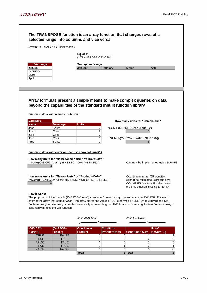
Syntax: =TRANSPOSE(data range )

Equation:

{=TRANSPOSE(C33:C36)}

data range Transposed range

January January February March April

February

March

April

Summing data with a single criterion

Database

Name Beverage Units

Josh Sprite 2

Josh Coke 2 5

Julia Coke 3

Josh Coke 1

Prue Sprite 1 5

Summing data with criterion that uses two columns(1)

How many units for "Name=Josh " and "Product=Coke "

{=SUM((C48:C52="Josh")*(D48:D52="Coke")*E48:E52)} Can now be implemented using SUMIFS

3

How many units for "Name=Josh " or "Product=Coke"

{=SUM(IF((C48:C52="Josh")+(D48:D52="Coke"),1,0)*E48:E52)}

8

How it works

Josh AND Coke Josh OR Coke

(C48:C52=

"Josh")

(D48:D52=

"coke")

Conditions

Product

Condition

Product*Units Conditions Sum

Units*

if(cSum1,0)

TRUE FALSE 0 0 1 2

TRUE TRUE 1 2 2 2

FALSE TRUE 0 0 1 3

TRUE TRUE 1 1 2 1

FALSE FALSE 0 0 0 0

Total 3 Total 8

The TRANSPOSE function is an array function that changes rows of a

selected range into columns and vice versa

The proportion of the formula (C48:C52="Josh ") creates a Boolean array, the same size as C48:C52. For each

entry of the array that equals "Josh " the array stores the value TRUE, otherwise FALSE. On multiplying the two

Boolean arrays a new array is created essentially representing the AND function. Summing the two Boolean arrays

essentially mimics the OR function.

Array formulas present a simple means to make complex queries on data,

beyond the capabilities of the standard inbuilt function library

How many units for "Name=Josh"

{=SUM(IF(C48:C52="Josh",E48:E52,0)})

=SUMIF(C48:C52,"Josh",E48:E52)

Counting using an OR condition

cannot be replicated using the new

COUNTIFS function. For this query

the only solution is using an array


Excel 2007 Training

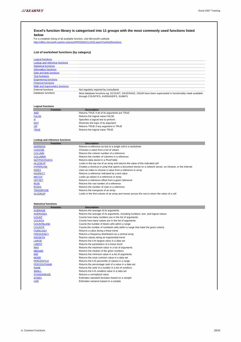
For a complete listing of all available function, visit Microsoft's website

http://office.microsoft.com/en-us/excel/HP052042111033.aspx#Text%20functions

Logical functions

Lookup and reference functions

Statistical functions

Information functions

Date and time functions

Text functions

Engineering functions

Financial functions

Math and trigonometry functions

External functions Not regularly required by consultants

Database functions

Function Description

AND

FALSE

IF

NOT

OR

TRUE


ADDRESS

CHOOSE

COLUMN

COLUMNS

GETPIVOTDATA

HLOOKUP

HYPERLINK

INDEX

INDIRECT

MATCH

OFFSET

ROW

ROWS

TRANSPOSE

VLOOKUP


AVERAGE

AVERAGEA

COUNT

COUNTA

COUNTBLANK

COUNTIF

FORECAST

FREQUENCY

GROWTH

LARGE

LINEST

MAX

MEDIAN

MIN

MODE

PERCENTILE

PERCENTRANK

RANK

SMALL

STANDARDIZE

STDEV

VAR

Returns TRUE if all of its arguments are TRUE

Returns the logical value FALSE

Specifies a logical test to perform

Reverses the logic of its argument

Returns TRUE if any argument is TRUE

Returns a reference as text to a single cell in a worksheet

Chooses a value from a list of values

Returns the column number of a reference

Returns the average of its arguments

Returns the average of its arguments, including numbers, text, and logical values

Counts how many numbers are in the list of arguments

Counts how many values are in the list of arguments

Returns the number of columns in a reference

Returns data stored in a PivotTable

Looks in the top row of an array and returns the value of the indicated cell

Creates a shortcut or jump that opens a document stored on a network server, an intranet, or the Internet

Uses an index to choose a value from a reference or array

Returns a reference indicated by a text value

Returns the k-th percentile of values in a range

Returns the percentage rank of a value in a data set

Returns the rank of a number in a list of numbers

Counts the number of blank cells within a range

Counts the number of nonblank cells within a range that meet the given criteria

Looks up values in a reference or array

Returns a reference offset from a given reference

Returns the row number of a reference

Returns the number of rows in a reference

Returns the transpose of an array

Looks in the first column of an array and moves across the row to return the value of a cell

Statistical functions

Returns a value along a linear trend

Returns a frequency distribution as a vertical array

Returns values along an exponential trend

Returns the k-th largest value in a data set

Returns the parameters of a linear trend

Returns the maximum value in a list of arguments

Returns the median of the given numbers

Returns the minimum value in a list of arguments

Returns the most common value in a data set

Returns the k-th smallest value in a data set

Returns a normalized value

Estimates standard deviation based on a sample

Estimates variance based on a sample

Excel's function library is categorised into 11 groups with the most commonly used functions listed

below

List of worksheet functions (by category)

Most database functions eg: DCOUNT, DAVERAGE, DSUM have been superseded in functionality made available

through COUNTIFS, AVERAGEIFS, SUMIFS

Logical functions

Returns the logical value TRUE

Lookup and reference functions

A. Common Functions 28/30

http://office.microsoft.com/en-us/excel/HP052042111033.aspx

Excel 2007 Training


CELL

ERROR.TYPE

ISBLANK

ISERR

ISERROR

ISEVEN

ISNA

ISNONTEXT

ISNUMBER

ISODD

ISTEXT

N


DATE

DAYS360

EOMONTH

HOUR

MONTH

NETWORKDAYS

NOW

TIME

TODAY

YEAR


CHAR

CLEAN

CONCATENATE

DOLLAR

EXACT

FIND, FINDB

FIXED

LEFT, LEFTB

LEN, LENB

LOWER

MID, MIDB

PROPER

REPLACE, REPLACEB

REPT

RIGHT, RIGHTB

SEARCH, SEARCHB

SUBSTITUTE

TEXT

TRIM

UPPER

VALUE

Example text: CapitalISes THE first LETTER in eAch woRd of a tExt vAlUe

=PROPER(D201) Capitalises The First Letter In Each Word Of A Text Value

=UPPER(LEFT(D201,1))&LOWER(RIGHT(D201,LEN(D201)-1)) Capitalises the first letter in each word of a text value

=TRIM(E205) Capitalises the first letter in each word of a text value


CONVERT

=CONVERT(1, "lbm", "kg")

Returns TRUE if the value is blank

Returns TRUE if the value is any error value except #N/A

Returns TRUE if the value is any error value

Returns TRUE if the number is even

Returns the serial number of the current date and time

Returns the serial number of a particular time

Returns a value converted to a number

Date and time functions

Returns information about the formatting, location, or contents of a cell

Returns a number corresponding to an error type

Information functions

Returns TRUE if the value is the #N/A error value

Returns TRUE if the value is not text

Returns TRUE if the value is a number

Returns TRUE if the number is odd

Returns TRUE if the value is text

Returns the serial number of today's date

Returns the character specified by the code number

Removes all nonprintable characters from text

Returns the serial number of a particular date

Calculates the number of days between two dates based on a 360-day year

Returns the serial number of the last day of the month before or after a specified number of months

Converts a serial number to an hour

Converts a serial number to a month

Returns the number of whole workdays between two dates

Repeats text a given number of times

Joins several text items into one text item

Converts a number to text, using the $ (dollar) currency format

Checks to see if two text values are identical

Finds one text value within another (case-sensitive)

Formats a number as text with a fixed number of decimals

Returns the leftmost characters from a text value

Returns the number of characters in a text string

Converts text to lowercase

Returns a specific number of characters from a text string starting at the position you specify

Capitalizes the first letter in each word of a text value

Replaces characters within text

Finds one text value within another (not case-sensitive)

Substitutes new text for old text in a text string

Formats a number and converts it to text

Removes spaces from text

Converts text to uppercase

Example

Converts 1 pound mass to kilograms

Converts a serial number to a year

Text functions

Converts a text argument to a number

Example - cure for Capitalisation disease

Engineering functions

Converts a number from one measurement system to another

Returns the rightmost characters from a text value


Excel 2007 Training


ACCRINT

ACCRINTM

AMORDEGRC

AMORLINC

DB

EFFECT

FV

NPV

PV

RATE

RECEIVED

XNPV

YIELD


ABS

CEILING

EXP

FLOOR

INT

LOG

LOG10

MMULT

MOD

MROUND

PI

POWER

PRODUCT

RAND

RANDBETWEEN

ROMAN

ROUND

SQRT

SUBTOTAL

SUM

SUMIF

SUMPRODUCT

Example Number: 3.141592654

=ROUND(D262,1) 3.1

=CEILING(D262,0.1) 3.2

=FLOOR(D262,0.1) 3.1

=MROUND(D262,0.01) 3.14

Returns the depreciation of an asset for a specified period by using the fixed-declining balance method

Returns the accrued interest for a security that pays periodic interest

Returns the accrued interest for a security that pays interest at maturity

Returns the depreciation for each accounting period by using a depreciation coefficient

Returns the depreciation for each accounting period

Rounds a number down to the nearest integer

Returns the logarithm of a number to a specified base

Returns the base-10 logarithm of a number

Rounds a number down, toward zero

Returns the effective annual interest rate

Returns the future value of an investment

Returns the net present value of an investment based on a series of periodic cash flows and a discount rate

Returns the present value of an investment

Returns the interest rate per period of an annuity

Returns the amount received at maturity for a fully invested security

Returns the net present value for a schedule of cash flows that is not necessarily periodic

Returns the absolute value of a number

Rounds a number to the nearest integer or to the nearest multiple of significance

Returns e raised to the power of a given number

Financial functions

Returns the yield on a security that pays periodic interest

Math and trigonometry functions

Returns the sum of the products of corresponding array components

Example

Returns the matrix product of two arrays

Returns the remainder from division

Returns a number rounded to the desired multiple

Returns the value of pi

Returns the result of a number raised to a power

Multiplies its arguments

Returns a random number between 0 and 1

Returns a random number between the numbers you specify

Converts an arabic numeral to roman, as text

Rounds a number to a specified number of digits

Returns a positive square root

Returns a subtotal in a list or database

Adds its arguments

Adds the cells specified by a given criteria


Documents

Excel Advanced Training