Excel 2007 Training Manual - ACUIA.org - Excel Training...Excel 2007 Training Manual ... Excel 2007 Training Manual ACUIA June 2013 Excel 2007 Page 2 ... to the area labeled Report

Excel 2007 Training Manual

Summarizing, Organizing, and Analyzing Large Sets of Data

Excel 2007 Training Manual ACUIA June 2013

Excel 2007 Page 2

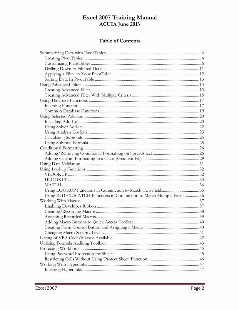
Table of Contents

Summarizing Data with PivotTables ............................................................................................ 4 Creating PivotTables .................................................................................................................. 4 Customizing PivotTables ........................................................................................................... 6 Drilling Down to Filtered Detail ............................................................................................ 11 Applying a Filter to Your PivotTable .................................................................................... 12 Sorting Data In PivotTable ..................................................................................................... 13

Using Advanced Filter .................................................................................................................. 13 Creating Advanced Filter ......................................................................................................... 13 Creating Advanced Filter With Multiple Criteria ................................................................. 15

Using Database Functions ........................................................................................................... 17 Inserting Function .................................................................................................................... 17 Common Database Functions ................................................................................................ 19

Using Selected Add-Ins ................................................................................................................ 20 Installing Add-Ins ..................................................................................................................... 20 Using Solver Add-in ................................................................................................................. 22 Using Analysis Toolpak ........................................................................................................... 23 Calculating Subtotals ................................................................................................................ 25 Using Subtotal Formula ........................................................................................................... 25

Conditional Formatting ................................................................................................................ 26 Adding/Removing Conditional Formatting on Spreadsheet ............................................. 26 Adding Custom Formatting to a Chart (Gradient Fill) ....................................................... 29

Using Data Validation ................................................................................................................... 31 Using Lookup Functions .............................................................................................................. 32

VLOOKUP ............................................................................................................................... 32 HLOOKUP ............................................................................................................................... 33 MATCH ..................................................................................................................................... 34 Using LOOKUP Functions in Conjunction to Match Two Fields ................................... 35 Using INDEX/MATCH Functions in Conjunction to Match Multiple Fields .............. 36

Working With Macros .................................................................................................................. 37 Enabling Developer Ribbon ................................................................................................... 37 Creating/Recording Macros .................................................................................................... 38 Accessing Recorded Macros .................................................................................................... 39 Adding Macro Buttons to Quick Access Toolbar ............................................................... 40 Creating Form Control Button and Assigning a Macro ...................................................... 40 Changing Macro Security Levels ............................................................................................. 41

Listing of VBA Code/Macros Available .................................................................................... 42 Utilizing Formula Auditing Toolbar ........................................................................................... 43 Protecting Workbook ................................................................................................................... 45

Using Password Protection for Sheets ................................................................................... 45 Restricting Cells Without Using ‗Protect Sheet‘ Function .................................................. 46

Working With Hyperlinks ............................................................................................................ 47 Inserting Hyperlinks ................................................................................................................. 47


Excel 2007 Page 3

Deleting Hyperlinks .................................................................................................................. 48 Editing Hyperlinks .................................................................................................................... 48

SUMPRODUCT and SUMIFS Formulas ................................................................................. 49 Calculating Loan Payment Streams with CUMPRINC and CUMINT ................................. 50 Performing Advanced Analysis in Excel .................................................................................... 52

Linear (Two-Factor) Regression Analysis ............................................................................. 52 Benford‘s Law Analysis ............................................................................................................ 54

Appendix A: Common Shortcut Keys ....................................................................................... 56


Excel 2007 Page 4

Summarizing Data with PivotTables

Creating PivotTables

1. Highlight all the cells in the list or database on which you wish to base the PivotTable Report (NOTE: EVERY column in your spreadsheet must have a heading in order to produce a PivotTable, or the report WILL NOT generate)

2. Click Insert > PivotTable to open the Create PivotTable dialog box (NOTE: Alternatively, you can use the Office 2003 shortcut key Alt+D, P to bring up the PivotTable Wizard)

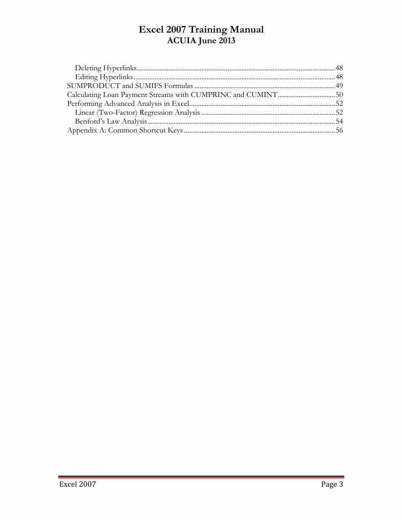
3. The ‗Select a table or range‘ and ‗New Worksheet‘ radio buttons are selected by default (see Exhibit 1-1). Click ‗OK‘, unless you would like to place the PivotTable in an existing worksheet.

EXHIBIT 1-1


Excel 2007 Page 5

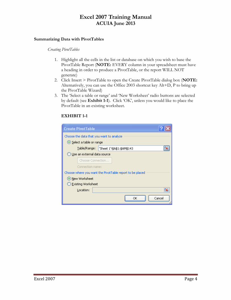
4. You will see a screen similar to the one in Exhibit 1-2: EXHIBIT 1-2

5. From the ‗PivotTable Field List‘ window, drag the fields with data that you want to display in rows to the drop area labeled ‗Row Labels‘ (NOTE: If you don't see the field list, click within the outlines of the PivotTable drop areas)

6. Drag fields with data that you want to display across columns to the drop area labeled ‗Column Labels‘

7. Drag fields that contain the data that you want to summarize to the area labeled ‗Values‘ (NOTE: If you add more than one data field, arrange these fields in the order you want by dragging them in order of desired priority)

8. Drag fields that you want to use as report filters (known as ‗page fields‘ in Office 2003) to the area labeled Report Filter (NOTE: This sort level is not commonly used)

9. To rearrange fields, drag them from one area to another 10. To remove a field, drag it out of the PivotTable report or uncheck the box in

the ‗Choose fields to add to the report‘ section above. 11. To hide the field list, click a cell outside the PivotTable report or select the

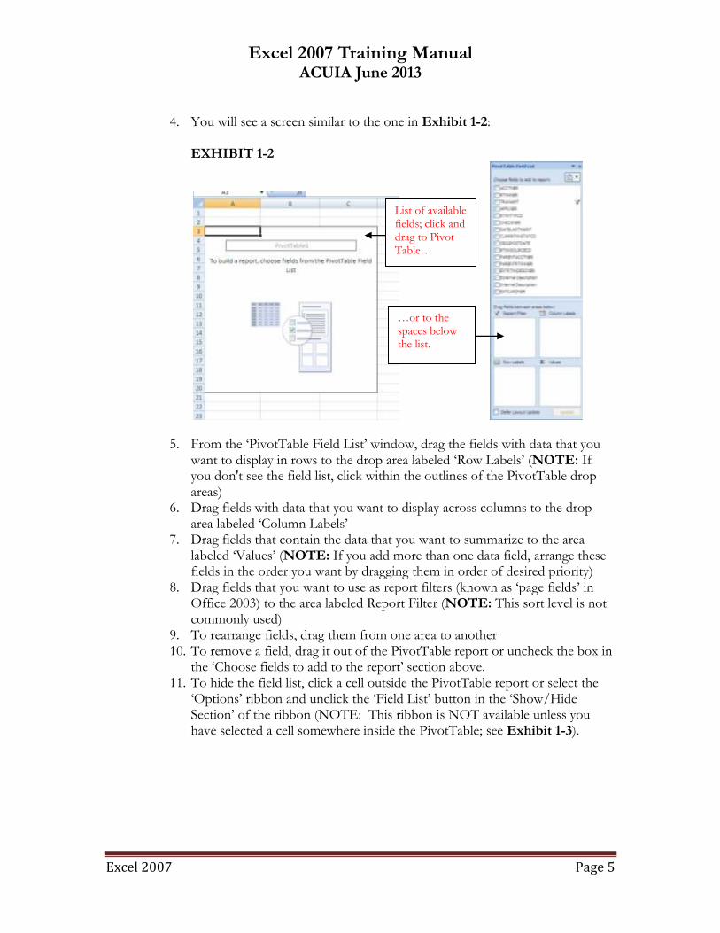
‗Options‘ ribbon and unclick the ‗Field List‘ button in the ‗Show/Hide Section‘ of the ribbon (NOTE: This ribbon is NOT available unless you have selected a cell somewhere inside the PivotTable; see Exhibit 1-3).

…or to the spaces below the list.

List of available fields; click and drag to Pivot Table…


Excel 2007 Page 6

EXHIBIT 1-3

12. To change order of items in ‗Row‘ fields, click and drag them up or down, as

desired. 13. To change the way the PivotTable summarizes the data in the ‗Values‘

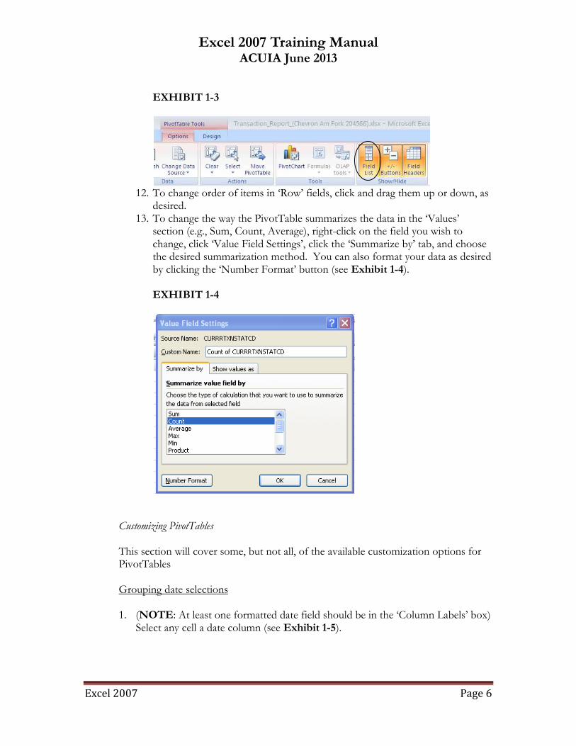
section (e.g., Sum, Count, Average), right-click on the field you wish to change, click ‗Value Field Settings‘, click the ‗Summarize by‘ tab, and choose the desired summarization method. You can also format your data as desired by clicking the ‗Number Format‘ button (see Exhibit 1-4). EXHIBIT 1-4

Customizing PivotTables

This section will cover some, but not all, of the available customization options for PivotTables

Grouping date selections 1. (NOTE: At least one formatted date field should be in the ‗Column Labels‘ box)

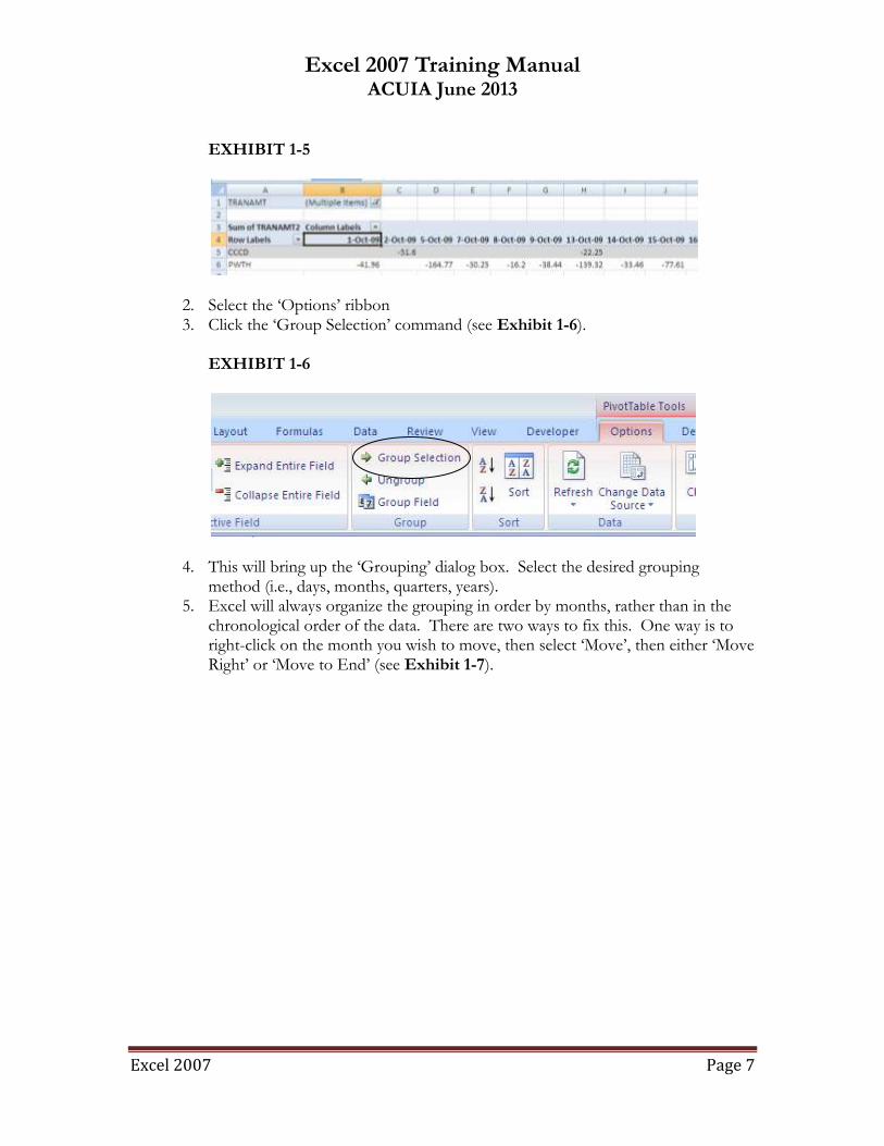
Select any cell a date column (see Exhibit 1-5).


Excel 2007 Page 7

EXHIBIT 1-5

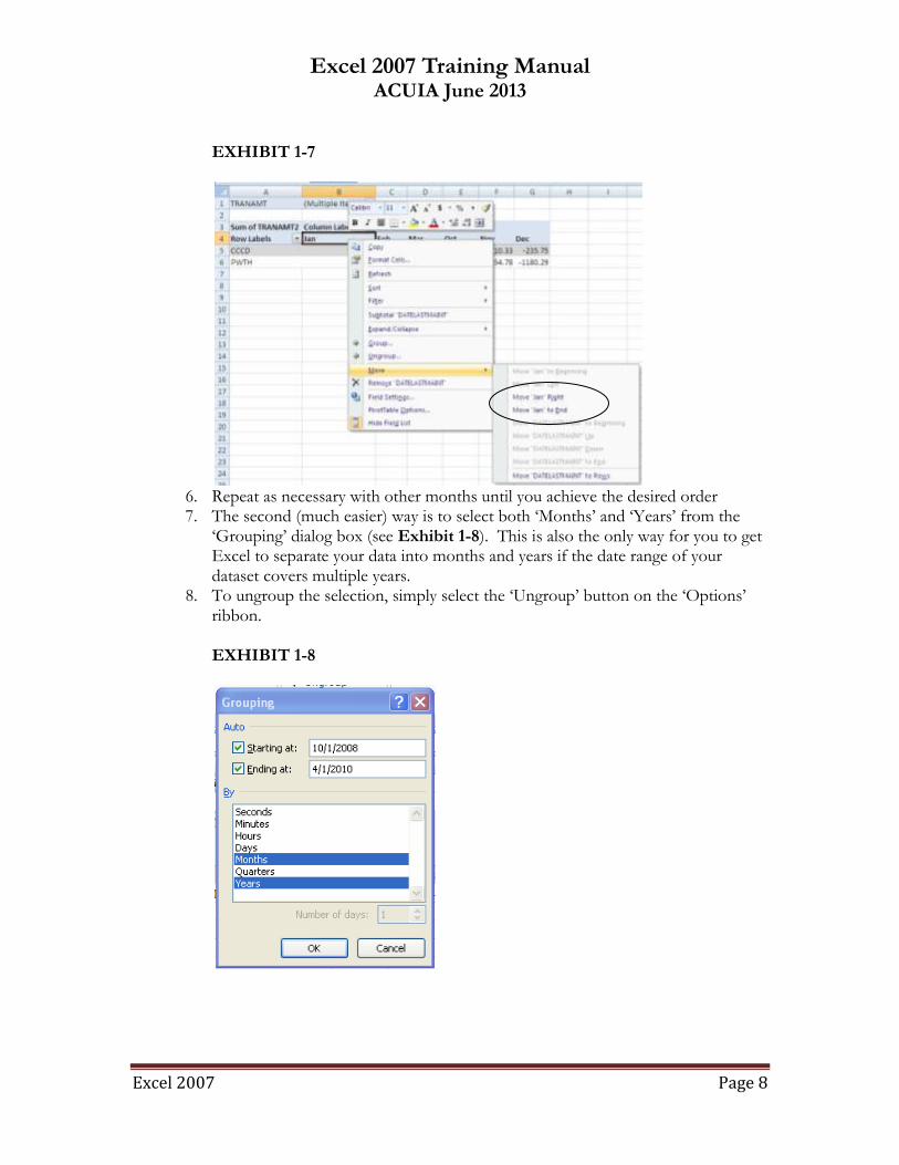
2. Select the ‗Options‘ ribbon 3. Click the ‗Group Selection‘ command (see Exhibit 1-6).

EXHIBIT 1-6

4. This will bring up the ‗Grouping‘ dialog box. Select the desired grouping method (i.e., days, months, quarters, years).

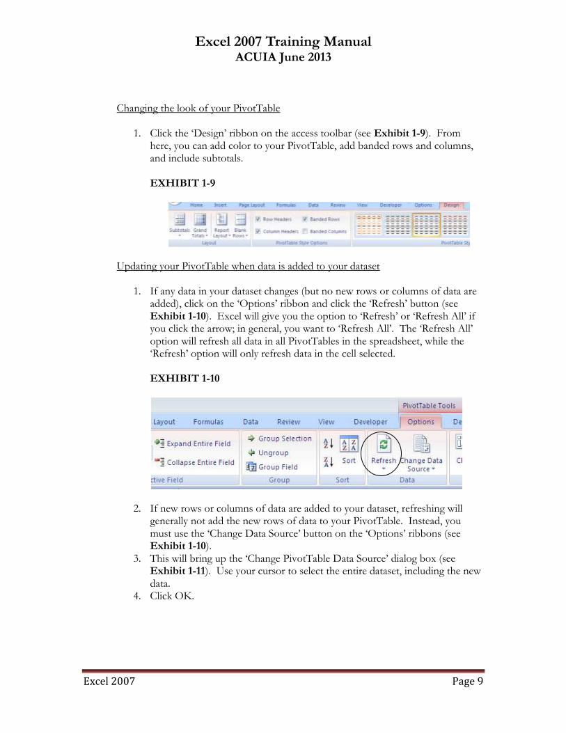
5. Excel will always organize the grouping in order by months, rather than in the chronological order of the data. There are two ways to fix this. One way is to right-click on the month you wish to move, then select ‗Move‘, then either ‗Move Right‘ or ‗Move to End‘ (see Exhibit 1-7).


Excel 2007 Page 8

EXHIBIT 1-7

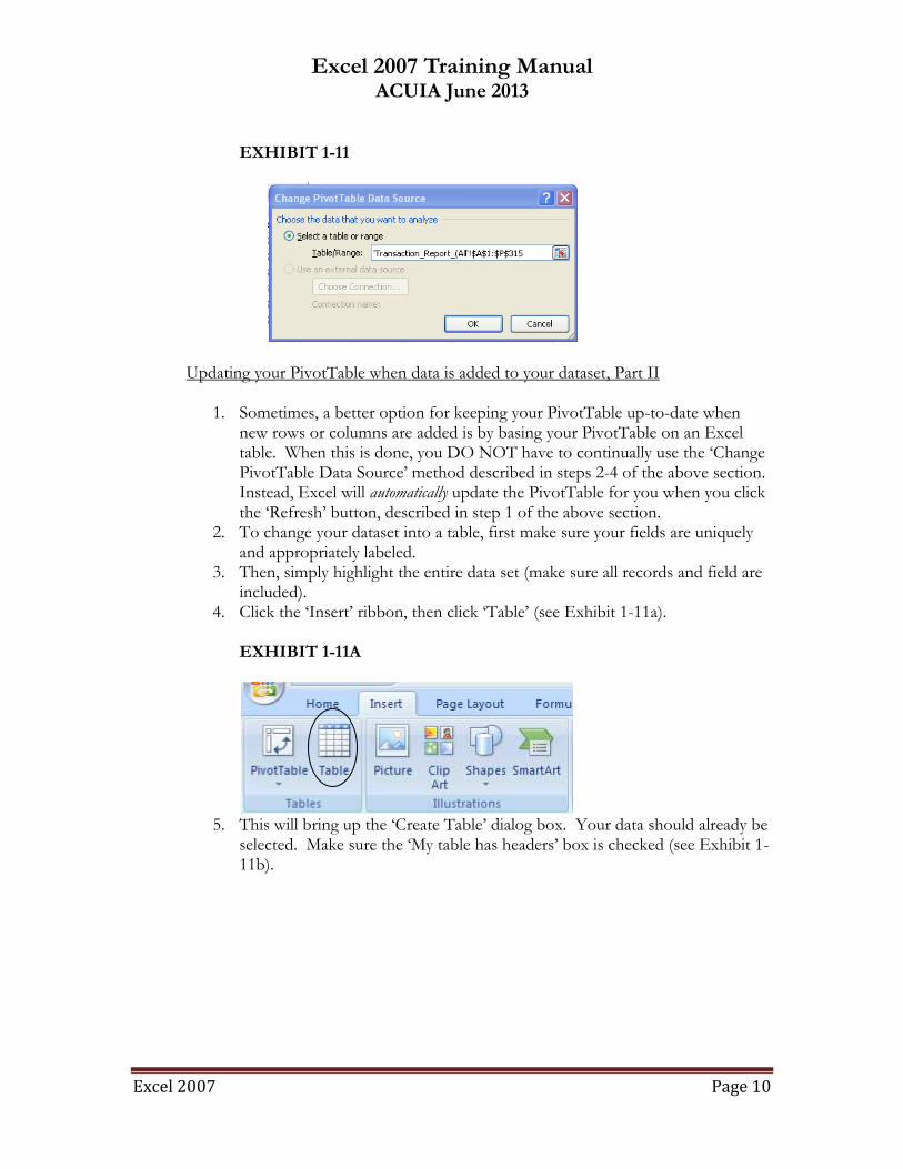
6. Repeat as necessary with other months until you achieve the desired order 7. The second (much easier) way is to select both ‗Months‘ and ‗Years‘ from the

‗Grouping‘ dialog box (see Exhibit 1-8). This is also the only way for you to get Excel to separate your data into months and years if the date range of your dataset covers multiple years.

8. To ungroup the selection, simply select the ‗Ungroup‘ button on the ‗Options‘ ribbon.

EXHIBIT 1-8


Excel 2007 Page 9

Changing the look of your PivotTable

1. Click the ‗Design‘ ribbon on the access toolbar (see Exhibit 1-9). From here, you can add color to your PivotTable, add banded rows and columns, and include subtotals.

EXHIBIT 1-9

Updating your PivotTable when data is added to your dataset

1. If any data in your dataset changes (but no new rows or columns of data are added), click on the ‗Options‘ ribbon and click the ‗Refresh‘ button (see Exhibit 1-10). Excel will give you the option to ‗Refresh‘ or ‗Refresh All‘ if you click the arrow; in general, you want to ‗Refresh All‘. The ‗Refresh All‘ option will refresh all data in all PivotTables in the spreadsheet, while the ‗Refresh‘ option will only refresh data in the cell selected. EXHIBIT 1-10

2. If new rows or columns of data are added to your dataset, refreshing will generally not add the new rows of data to your PivotTable. Instead, you must use the ‗Change Data Source‘ button on the ‗Options‘ ribbons (see Exhibit 1-10).

3. This will bring up the ‗Change PivotTable Data Source‘ dialog box (see Exhibit 1-11). Use your cursor to select the entire dataset, including the new data.

4. Click OK.


Excel 2007 Page 10

EXHIBIT 1-11

Updating your PivotTable when data is added to your dataset, Part II

1. Sometimes, a better option for keeping your PivotTable up-to-date when new rows or columns are added is by basing your PivotTable on an Excel table. When this is done, you DO NOT have to continually use the ‗Change PivotTable Data Source‘ method described in steps 2-4 of the above section. Instead, Excel will automatically update the PivotTable for you when you click the ‗Refresh‘ button, described in step 1 of the above section.

2. To change your dataset into a table, first make sure your fields are uniquely and appropriately labeled.

3. Then, simply highlight the entire data set (make sure all records and field are included).

4. Click the ‗Insert‘ ribbon, then click ‗Table‘ (see Exhibit 1-11a). EXHIBIT 1-11A

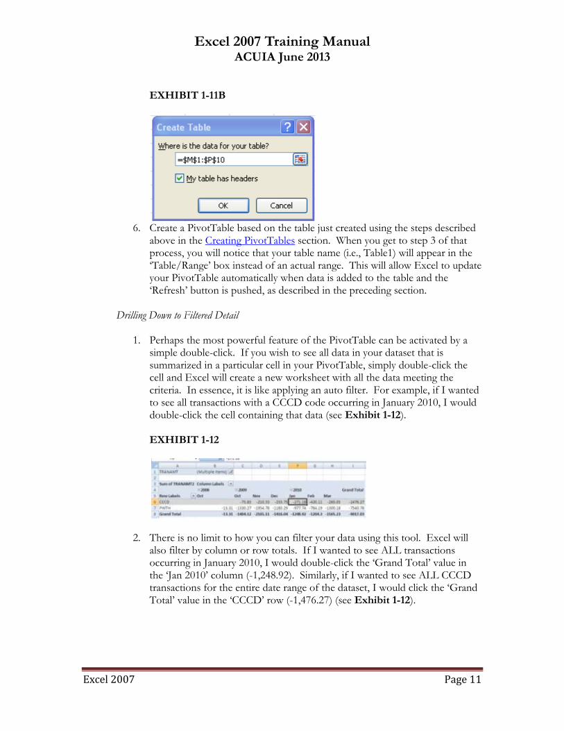
5. This will bring up the ‗Create Table‘ dialog box. Your data should already be

selected. Make sure the ‗My table has headers‘ box is checked (see Exhibit 1-11b).


Excel 2007 Page 11

EXHIBIT 1-11B

6. Create a PivotTable based on the table just created using the steps described

above in the Creating PivotTables section. When you get to step 3 of that process, you will notice that your table name (i.e., Table1) will appear in the ‗Table/Range‘ box instead of an actual range. This will allow Excel to update your PivotTable automatically when data is added to the table and the ‗Refresh‘ button is pushed, as described in the preceding section.

Drilling Down to Filtered Detail

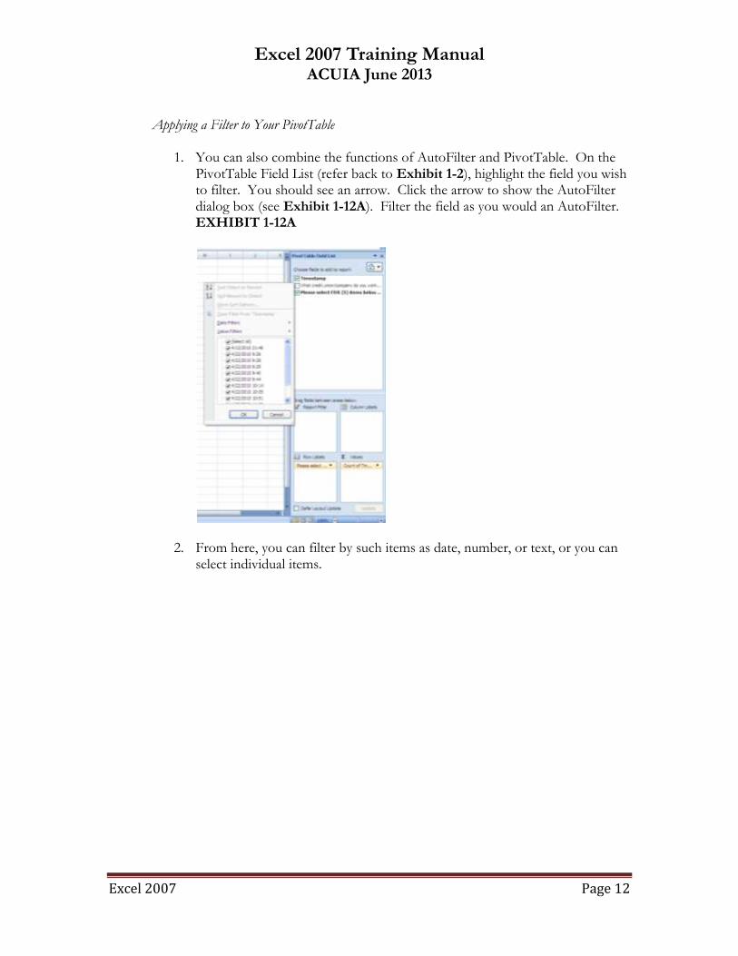
1. Perhaps the most powerful feature of the PivotTable can be activated by a

simple double-click. If you wish to see all data in your dataset that is summarized in a particular cell in your PivotTable, simply double-click the cell and Excel will create a new worksheet with all the data meeting the criteria. In essence, it is like applying an auto filter. For example, if I wanted to see all transactions with a CCCD code occurring in January 2010, I would double-click the cell containing that data (see Exhibit 1-12). EXHIBIT 1-12

2. There is no limit to how you can filter your data using this tool. Excel will also filter by column or row totals. If I wanted to see ALL transactions occurring in January 2010, I would double-click the ‗Grand Total‘ value in the ‗Jan 2010‘ column (-1,248.92). Similarly, if I wanted to see ALL CCCD transactions for the entire date range of the dataset, I would click the ‗Grand Total‘ value in the ‗CCCD‘ row (-1,476.27) (see Exhibit 1-12).


Excel 2007 Page 12

Applying a Filter to Your PivotTable

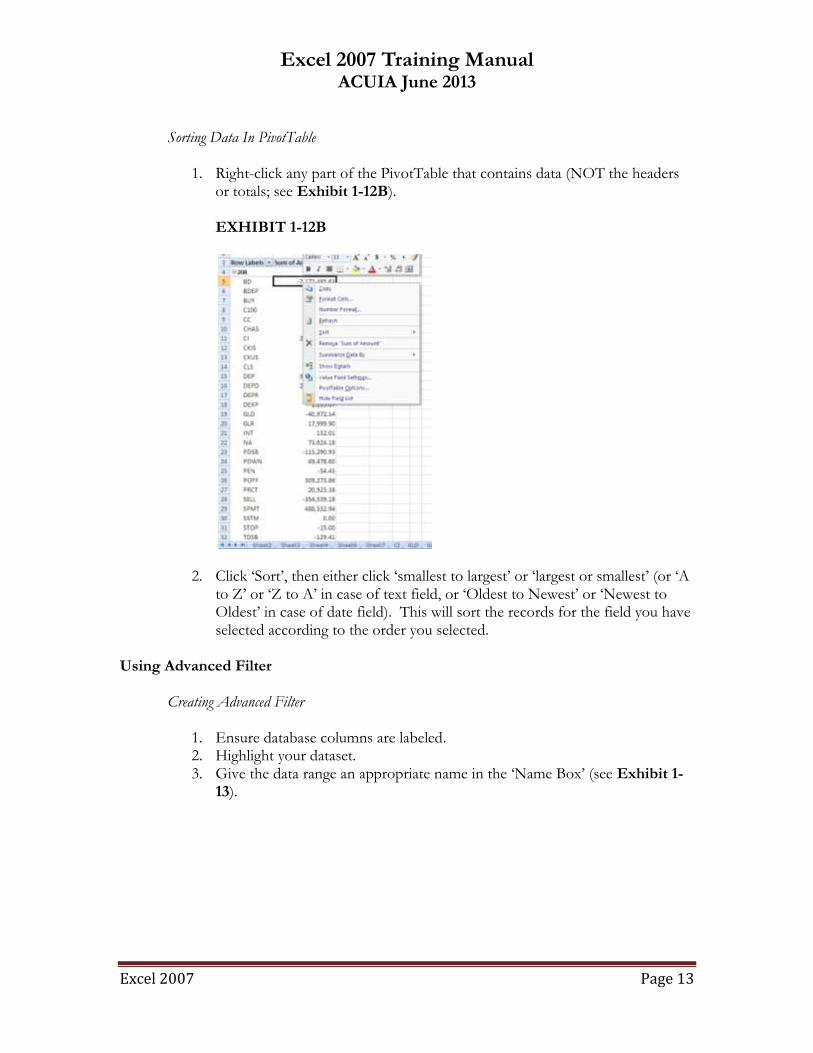
1. You can also combine the functions of AutoFilter and PivotTable. On the PivotTable Field List (refer back to Exhibit 1-2), highlight the field you wish to filter. You should see an arrow. Click the arrow to show the AutoFilter dialog box (see Exhibit 1-12A). Filter the field as you would an AutoFilter. EXHIBIT 1-12A

2. From here, you can filter by such items as date, number, or text, or you can select individual items.


Excel 2007 Page 13

Sorting Data In PivotTable

1. Right-click any part of the PivotTable that contains data (NOT the headers or totals; see Exhibit 1-12B). EXHIBIT 1-12B

2. Click ‗Sort‘, then either click ‗smallest to largest‘ or ‗largest or smallest‘ (or ‗A to Z‘ or ‗Z to A‘ in case of text field, or ‗Oldest to Newest‘ or ‗Newest to Oldest‘ in case of date field). This will sort the records for the field you have selected according to the order you selected.

Using Advanced Filter

Creating Advanced Filter

1. Ensure database columns are labeled. 2. Highlight your dataset. 3. Give the data range an appropriate name in the ‗Name Box‘ (see Exhibit 1-

13).


Excel 2007 Page 14

EXHIBIT 1-13

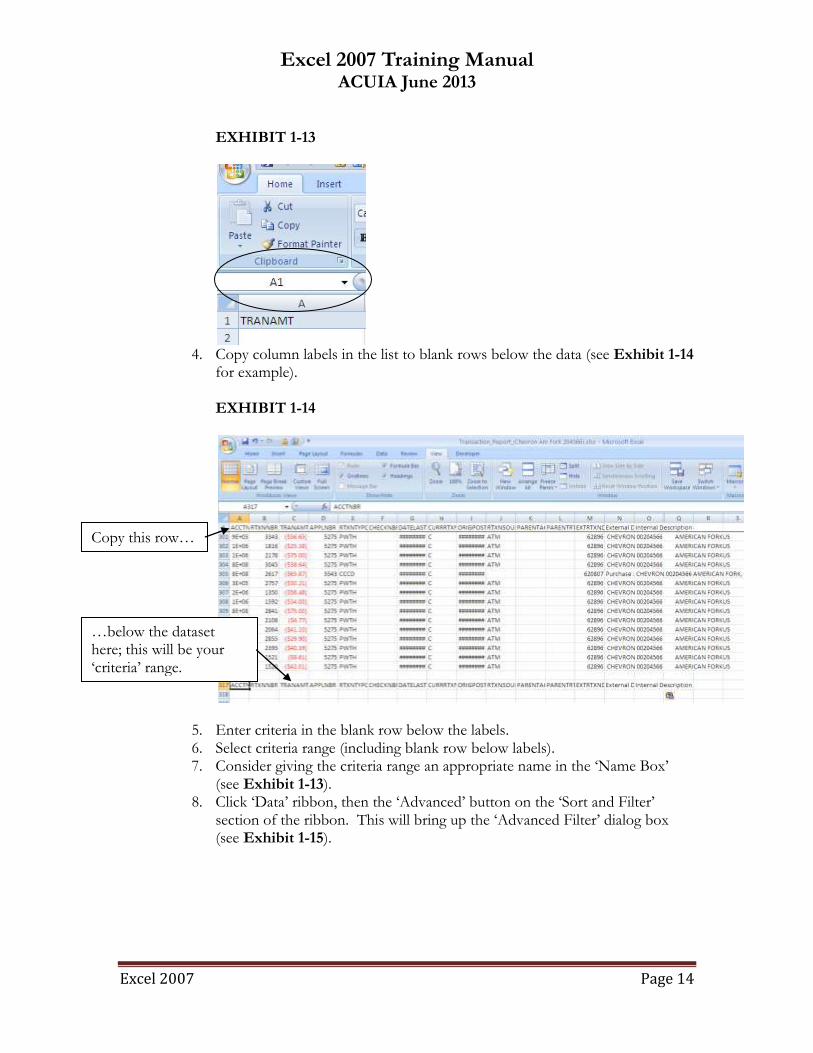
4. Copy column labels in the list to blank rows below the data (see Exhibit 1-14

for example). EXHIBIT 1-14

5. Enter criteria in the blank row below the labels. 6. Select criteria range (including blank row below labels). 7. Consider giving the criteria range an appropriate name in the ‗Name Box‘

(see Exhibit 1-13). 8. Click ‗Data‘ ribbon, then the ‗Advanced‘ button on the ‗Sort and Filter‘

section of the ribbon. This will bring up the ‗Advanced Filter‘ dialog box (see Exhibit 1-15).

Copy this row…

…below the dataset here; this will be your ‗criteria‘ range.


Excel 2007 Page 15

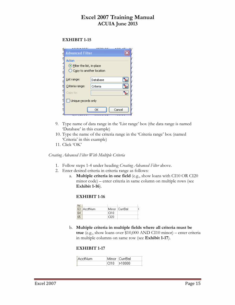
EXHIBIT 1-15

9. Type name of data range in the ‗List range‘ box (the data range is named ‗Database‘ in this example)

10. Type the name of the criteria range in the ‗Criteria range‘ box (named ‗Criteria‘ in this example)

11. Click ‗OK‘ Creating Advanced Filter With Multiple Criteria

1. Follow steps 1-4 under heading Creating Advanced Filter above. 2. Enter desired criteria in criteria range as follows:

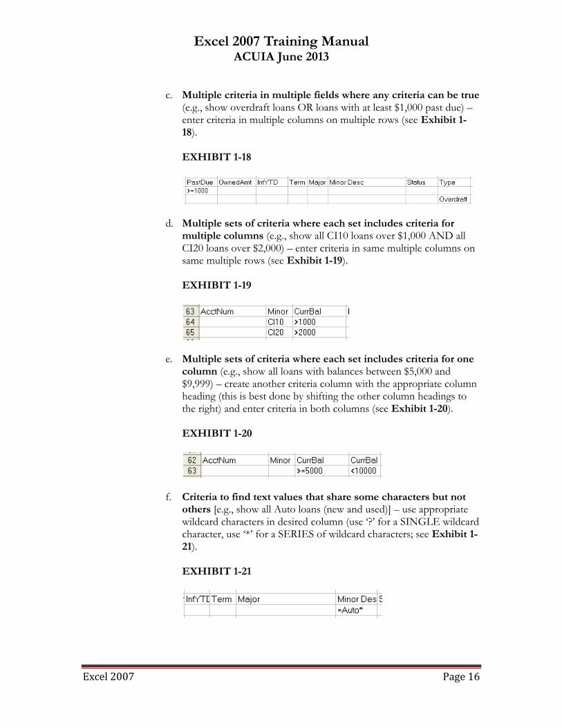
a. Multiple criteria in one field (e.g., show loans with CI10 OR CI20 minor code) – enter criteria in same column on multiple rows (see Exhibit 1-16).

EXHIBIT 1-16

b. Multiple criteria in multiple fields where all criteria must be true (e.g., show loans over $10,000 AND CI10 minor) – enter criteria in multiple columns on same row (see Exhibit 1-17). EXHIBIT 1-17


Excel 2007 Page 16

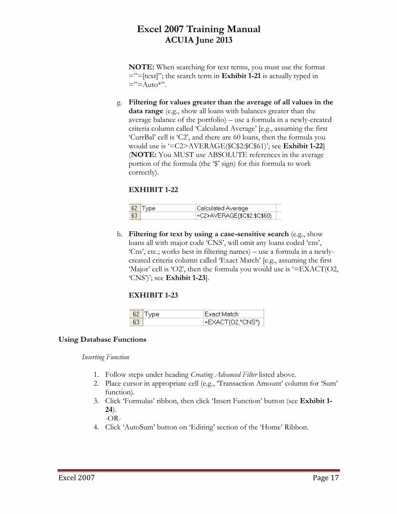
c. Multiple criteria in multiple fields where any criteria can be true (e.g., show overdraft loans OR loans with at least $1,000 past due) – enter criteria in multiple columns on multiple rows (see Exhibit 1-18).

EXHIBIT 1-18

d. Multiple sets of criteria where each set includes criteria for multiple columns (e.g., show all CI10 loans over $1,000 AND all CI20 loans over $2,000) – enter criteria in same multiple columns on same multiple rows (see Exhibit 1-19). EXHIBIT 1-19

e. Multiple sets of criteria where each set includes criteria for one column (e.g., show all loans with balances between $5,000 and $9,999) – create another criteria column with the appropriate column heading (this is best done by shifting the other column headings to the right) and enter criteria in both columns (see Exhibit 1-20). EXHIBIT 1-20

f. Criteria to find text values that share some characters but not others [e.g., show all Auto loans (new and used)] – use appropriate wildcard characters in desired column (use ‗?‘ for a SINGLE wildcard character, use ‗*‘ for a SERIES of wildcard characters; see Exhibit 1-21). EXHIBIT 1-21


Excel 2007 Page 17

NOTE: When searching for text terms, you must use the format =‖=[text]‖; the search term in Exhibit 1-21 is actually typed in =‖=Auto*‖.

g. Filtering for values greater than the average of all values in the data range (e.g., show all loans with balances greater than the average balance of the portfolio) – use a formula in a newly-created criteria column called ‗Calculated Average‘ [e.g., assuming the first ‗CurrBal‘ cell is ‗C2‘, and there are 60 loans, then the formula you would use is ‗=C2>AVERAGE($C$2:$C$61)‘; see Exhibit 1-22] (NOTE: You MUST use ABSOLUTE references in the average portion of the formula (the ‗$‘ sign) for this formula to work correctly). EXHIBIT 1-22

h. Filtering for text by using a case-sensitive search (e.g., show loans all with major code ‗CNS‘, will omit any loans coded ‗cns‘, ‗Cns‘, etc.; works best in filtering names) – use a formula in a newly-created criteria column called ‗Exact Match‘ [e.g., assuming the first ‗Major‘ cell is ‗O2‘, then the formula you would use is ‗=EXACT(O2, ‗CNS‘)‘; see Exhibit 1-23]. EXHIBIT 1-23

Using Database Functions

Inserting Function

1. Follow steps under heading Creating Advanced Filter listed above. 2. Place cursor in appropriate cell (e.g., ‗Transaction Amount‘ column for ‗Sum‘

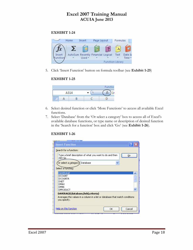
function). 3. Click ‗Formulas‘ ribbon, then click ‗Insert Function‘ button (see Exhibit 1-

24). -OR-

4. Click ‗AutoSum‘ button on ‗Editing‘ section of the ‗Home‘ Ribbon.


Excel 2007 Page 18

EXHIBIT 1-24

5. Click ‗Insert Function‘ button on formula toolbar (see Exhibit 1-25)

EXHIBIT 1-25

6. Select desired function or click ‗More Functions‘ to access all available Excel functions.

7. Select ‗Database‘ from the ‗Or select a category‘ box to access all of Excel‘s available database functions, or type name or description of desired function in the ‗Search for a function‘ box and click ‗Go‘ (see Exhibit 1-26). EXHIBIT 1-26


Excel 2007 Page 19

Common Database Functions

1. DSUM(database,field,criteria) – Returns sum of amounts in specified field based on appointed criteria (NOTE: For functions, if you named the cells, you can use the name you assigned the database and the criteria in the appropriate section of the equation).

2. DAVERAGE(database,field,criteria) – Returns average of amounts in specified field based on appointed criteria.

3. DCOUNT(database,field,criteria) – Returns count of records in specified field based on appointed criteria.

4. DSTDEV(database,field,criteria) – Returns standard deviation of records in specified field based on appointed criteria.

5. DGET(database,field,criteria) – Returns value of field of single record based on appointed criteria (e.g., what is the interest rate of the loan with a current balance of $4,234.29).


Excel 2007 Page 20

Using Selected Add-Ins

Installing Add-Ins 1. Click the ‗Office Button‘ in the upper left hand corner of the spreadsheet

(see Exhibit 1-27). EXHIBIT 1-27

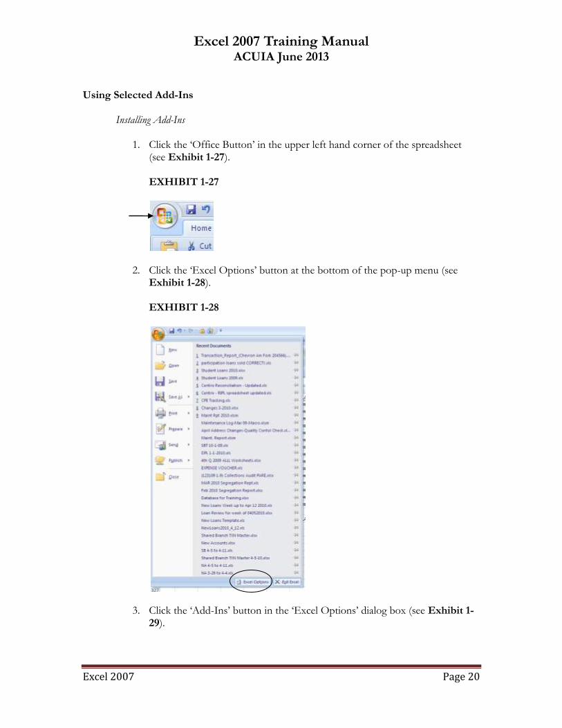
2. Click the ‗Excel Options‘ button at the bottom of the pop-up menu (see Exhibit 1-28).

EXHIBIT 1-28

3. Click the ‗Add-Ins‘ button in the ‗Excel Options‘ dialog box (see Exhibit 1-29).


Excel 2007 Page 21

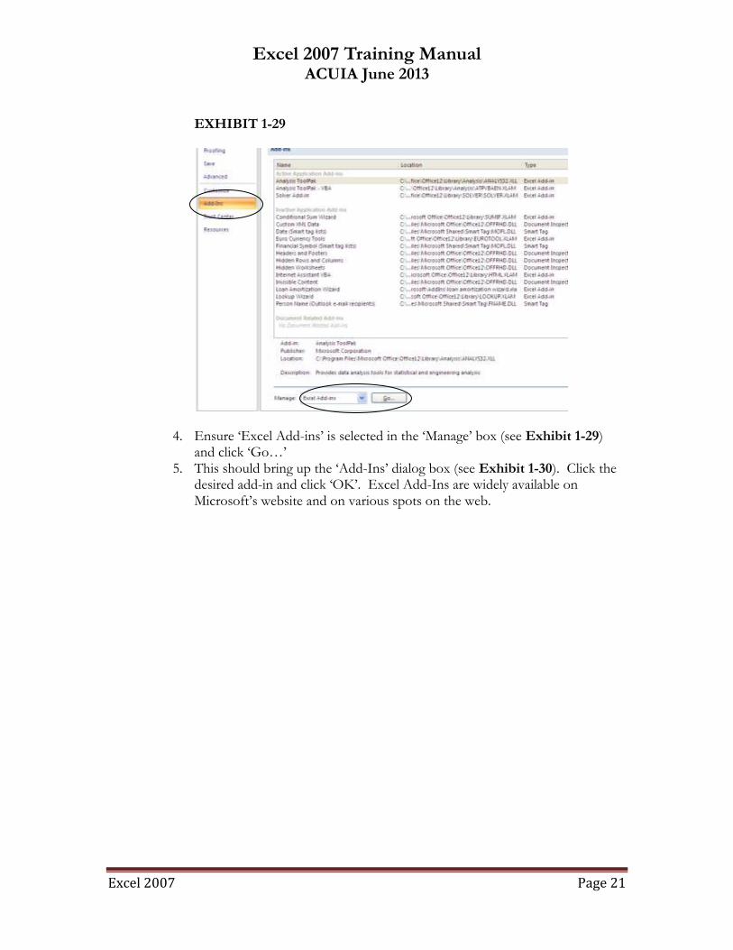
EXHIBIT 1-29

4. Ensure ‗Excel Add-ins‘ is selected in the ‗Manage‘ box (see Exhibit 1-29) and click ‗Go…‘

5. This should bring up the ‗Add-Ins‘ dialog box (see Exhibit 1-30). Click the desired add-in and click ‗OK‘. Excel Add-Ins are widely available on Microsoft‘s website and on various spots on the web.


Excel 2007 Page 22

EXHIBIT 1-30

Using Solver Add-in

1. Ensure the add-in has been installed following the steps listed in the Installing Add-Ins heading above.

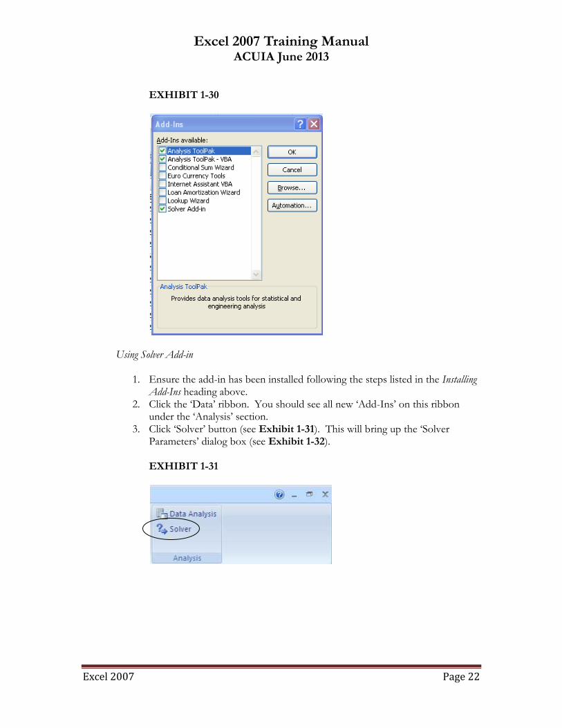
2. Click the ‗Data‘ ribbon. You should see all new ‗Add-Ins‘ on this ribbon under the ‗Analysis‘ section.

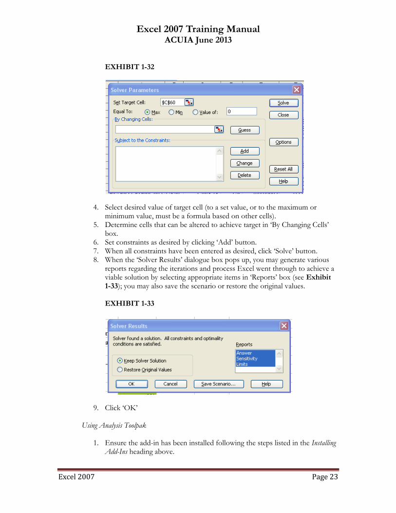
3. Click ‗Solver‘ button (see Exhibit 1-31). This will bring up the ‗Solver Parameters‘ dialog box (see Exhibit 1-32).

EXHIBIT 1-31


Excel 2007 Page 23

EXHIBIT 1-32

4. Select desired value of target cell (to a set value, or to the maximum or minimum value, must be a formula based on other cells).

5. Determine cells that can be altered to achieve target in ‗By Changing Cells‘ box.

6. Set constraints as desired by clicking ‗Add‘ button. 7. When all constraints have been entered as desired, click ‗Solve‘ button. 8. When the ‗Solver Results‘ dialogue box pops up, you may generate various

reports regarding the iterations and process Excel went through to achieve a viable solution by selecting appropriate items in ‗Reports‘ box (see Exhibit 1-33); you may also save the scenario or restore the original values. EXHIBIT 1-33

9. Click ‗OK‘

Using Analysis Toolpak

1. Ensure the add-in has been installed following the steps listed in the Installing Add-Ins heading above.


Excel 2007 Page 24

2. Click the ‗Data‘ ribbon. You should see all new ‗Add-Ins‘ on this ribbon under the ‗Analysis‘ section.

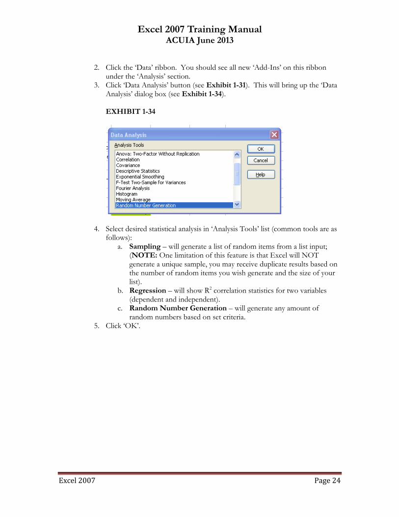
3. Click ‗Data Analysis‘ button (see Exhibit 1-31). This will bring up the ‗Data Analysis‘ dialog box (see Exhibit 1-34).

EXHIBIT 1-34

4. Select desired statistical analysis in ‗Analysis Tools‘ list (common tools are as follows):

a. Sampling – will generate a list of random items from a list input; (NOTE: One limitation of this feature is that Excel will NOT generate a unique sample, you may receive duplicate results based on the number of random items you wish generate and the size of your list).

b. Regression – will show R2 correlation statistics for two variables (dependent and independent).

c. Random Number Generation – will generate any amount of random numbers based on set criteria.

5. Click ‗OK‘.


Excel 2007 Page 25

Calculating Subtotals

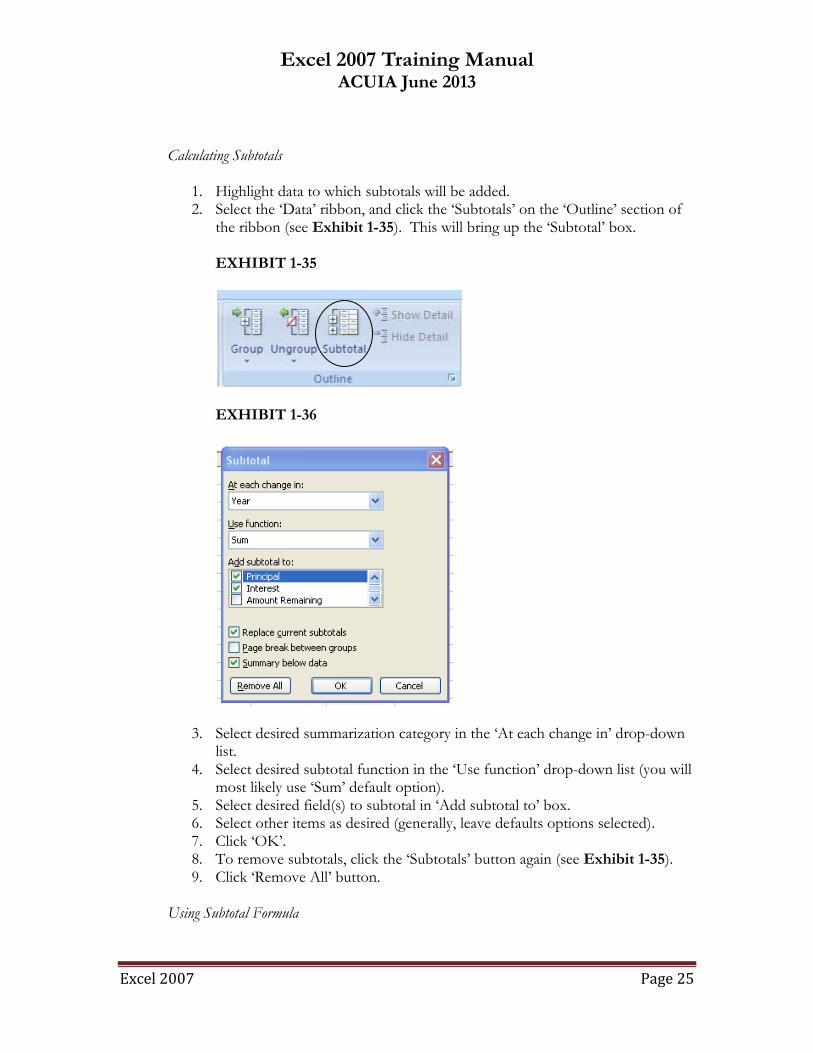
1. Highlight data to which subtotals will be added. 2. Select the ‗Data‘ ribbon, and click the ‗Subtotals‘ on the ‗Outline‘ section of

the ribbon (see Exhibit 1-35). This will bring up the ‗Subtotal‘ box. EXHIBIT 1-35

EXHIBIT 1-36

3. Select desired summarization category in the ‗At each change in‘ drop-down list.

4. Select desired subtotal function in the ‗Use function‘ drop-down list (you will most likely use ‗Sum‘ default option).

5. Select desired field(s) to subtotal in ‗Add subtotal to‘ box. 6. Select other items as desired (generally, leave defaults options selected). 7. Click ‗OK‘. 8. To remove subtotals, click the ‗Subtotals‘ button again (see Exhibit 1-35). 9. Click ‗Remove All‘ button.

Using Subtotal Formula


Excel 2007 Page 26

1. In addition to the method described above, subtotals can also be added using a formula. This is sometimes an easier method to use if Excel cannot tell what data set you are trying to subtotal, or if you don‘t want the three subtotal layers added by using the ‗Subtotal‘ button on the ribbon.

2. The formula is ―=SUBTOTAL([function number], [range reference])‖ and is composed of the following elements:

a. Function number: tells Excel what type of subtotal you wish to apply.

b. Range reference: range to which you wish to add a subtotal. 3. Use any of the following numbers for the function number:

a. 1 = Average b. 2 = Count c. 3 = CountA (count non-blank cells) d. 4 = Maximum e. 5 = Minimum f. 6 = Product (multiplies all values, not used often) g. 7 = Standard Deviation (Sample) h. 8 = Standard Deviation (Population) i. 9 = Sum j. 10 = Variance (Sample) k. 11 = Variance (Population)

4. Select the column of data you wish to summarize for the second portion of the formula (range reference).

5. Apply desired filters to the data to show appropriate summaries by the filter or filters you applied.

Conditional Formatting One of Excel‘s most powerful and aesthetically pleasing tools is conditional formatting. This tool is especially useful for quickly pinpointing outliers in matrices of data. Here are a few ways to use conditional formatting.

Adding/Removing Conditional Formatting on Spreadsheet

1. Highlight the data set you wish to conditionally format. 2. On the ‗Home‘ ribbon, click on the ‗Conditional Formatting‘ button.


Excel 2007 Page 27

EXHIBIT 1-37

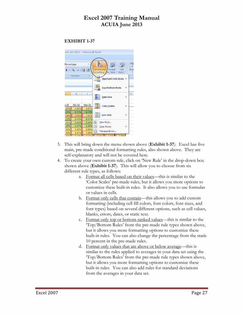
3. This will bring down the menu shown above (Exhibit 1-37). Excel has five main, pre-made conditional formatting rules, also shown above. They are self-explanatory and will not be covered here.

4. To create your own custom rule, click on ‗New Rule‘ in the drop-down box shown above (Exhibit 1-37). This will allow you to choose from six different rule types, as follows:

a. Format all cells based on their values—this is similar to the ‗Color Scales‘ pre-made rules, but it allows you more options to customize these built-in rules. It also allows you to use formulas or values in cells.

b. Format only cells that contain—this allows you to add custom formatting (including cell fill colors, font colors, font sizes, and font types) based on several different options, such as cell values, blanks, errors, dates, or static text.

c. Format only top or bottom ranked values—this is similar to the ‗Top/Bottom Rules‘ from the pre-made rule types shown above, but it allows you more formatting options to customize these built-in rules. You can also change the percentage from the static 10 percent in the pre-made rules.

d. Format only values that are above or below average—this is similar to the rules applied to averages in your data set using the ‗Top/Bottom Rules‘ from the pre-made rule types shown above, but it allows you more formatting options to customize these built-in rules. You can also add rules for standard deviations from the averages in your data set.


Excel 2007 Page 28

e. Format only unique or duplicate values— this allows you to add custom formatting (including cell fill colors, font colors, font sizes, and font types) to all unique or duplicate values in your data set.

f. Use a formula to determine which cells to format—this allows you to format your cells contingent upon a formula. Use this option if you have a complex formula that is not possible using the ‗Format only cells that contain‘ option.

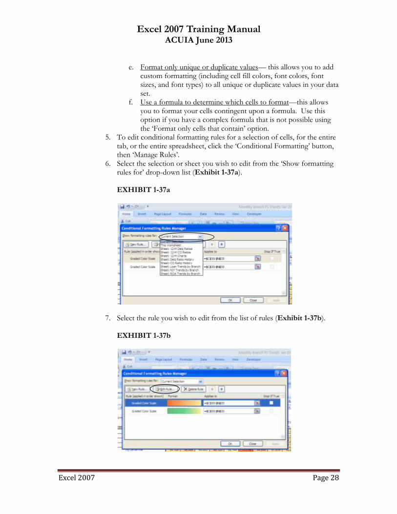
5. To edit conditional formatting rules for a selection of cells, for the entire tab, or the entire spreadsheet, click the ‗Conditional Formatting‘ button, then ‗Manage Rules‘.

6. Select the selection or sheet you wish to edit from the ‗Show formatting rules for‘ drop-down list (Exhibit 1-37a). EXHIBIT 1-37a

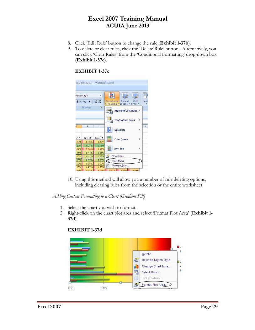
7. Select the rule you wish to edit from the list of rules (Exhibit 1-37b). EXHIBIT 1-37b


Excel 2007 Page 29

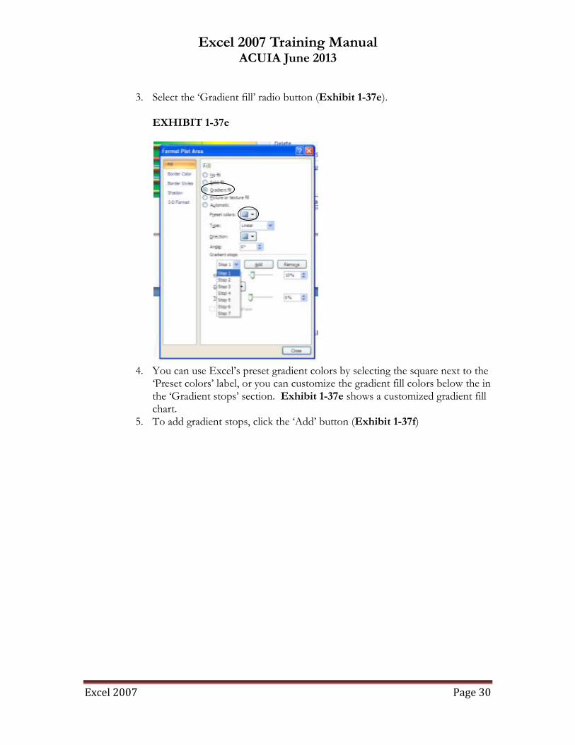
8. Click ‗Edit Rule‘ button to change the rule (Exhibit 1-37b). 9. To delete or clear rules, click the ‗Delete Rule‘ button. Alternatively, you

can click ‗Clear Rules‘ from the ‗Conditional Formatting‘ drop-down box (Exhibit 1-37c). EXHIBIT 1-37c

10. Using this method will allow you a number of rule deleting options, including clearing rules from the selection or the entire worksheet.

Adding Custom Formatting to a Chart (Gradient Fill)

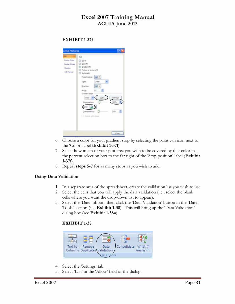
1. Select the chart you wish to format. 2. Right-click on the chart plot area and select ‗Format Plot Area‘ (Exhibit 1-

37d). EXHIBIT 1-37d


Excel 2007 Page 30

3. Select the ‗Gradient fill‘ radio button (Exhibit 1-37e). EXHIBIT 1-37e

4. You can use Excel‘s preset gradient colors by selecting the square next to the

‗Preset colors‘ label, or you can customize the gradient fill colors below the in the ‗Gradient stops‘ section. Exhibit 1-37e shows a customized gradient fill chart.

5. To add gradient stops, click the ‗Add‘ button (Exhibit 1-37f)


Excel 2007 Page 31

EXHIBIT 1-37f

6. Choose a color for your gradient stop by selecting the paint can icon next to

the ‗Color‘ label (Exhibit 1-37f). 7. Select how much of your plot area you wish to be covered by that color in

the percent selection box to the far right of the ‗Stop position‘ label (Exhibit 1-37f).

8. Repeat steps 5-7 for as many stops as you wish to add. Using Data Validation

1. In a separate area of the spreadsheet, create the validation list you wish to use 2. Select the cells that you will apply the data validation (i.e., select the blank

cells where you want the drop-down list to appear). 3. Select the ‗Data‘ ribbon, then click the ‗Data Validation‘ button in the ‗Data

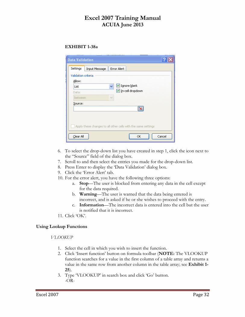
Tools‘ section (see Exhibit 1-38). This will bring up the ‗Data Validation‘ dialog box (see Exhibit 1-38a). EXHIBIT 1-38

4. Select the ‗Settings‘ tab. 5. Select ‗List‘ in the ‗Allow‘ field of the dialog.


Excel 2007 Page 32

EXHIBIT 1-38a

6. To select the drop-down list you have created in step 1, click the icon next to the ―Source‖ field of the dialog box.

7. Scroll to and then select the entries you made for the drop-down list. 8. Press Enter to display the ‗Data Validation‘ dialog box. 9. Click the ‗Error Alert‘ tab. 10. For the error alert, you have the following three options:

a. Stop—The user is blocked from entering any data in the cell except for the data required.

b. Warning—The user is warned that the data being entered is incorrect, and is asked if he or she wishes to proceed with the entry.

c. Information—The incorrect data is entered into the cell but the user is notified that it is incorrect.

11. Click ‗OK‘. Using Lookup Functions

VLOOKUP

1. Select the cell in which you wish to insert the function. 2. Click ‗Insert function‘ button on formula toolbar (NOTE: The VLOOKUP

function searches for a value in the first column of a table array and returns a value in the same row from another column in the table array; see Exhibit 1-25).

3. Type ‗VLOOKUP‘ in search box and click ‗Go‘ button. -OR-


Excel 2007 Page 33

4. Type the formula directly in cell; syntax for this formula is VLOOKUP(lookup_value,table_array,col_index_num,range_lookup), with each element defined as follows:

a. Lookup_value—The value to search in the first column of the table array. Lookup_value can be a value or a reference. If lookup_value is smaller than the smallest value in the first column of table_array, VLOOKUP returns the #N/A error value.

b. Table_array—Two or more columns of data. Use a reference to a range or a range name. The values in the first column of table_array are the values searched by lookup_value. These values can be text, numbers, or logical values. Uppercase and lowercase text are equivalent

c. Col_index_num—The column number in table_array from which the matching value must be returned. A col_index_num of 1 returns the value in the first column in table_array; a col_index_num of 2 returns the value in the second column in table_array, and so on. If col_index_num is:

i. Less than 1, VLOOKUP returns the #VALUE! error value ii. Greater than the number of columns in table_array,

VLOOKUP returns the #REF! error value. d. Range_lookup – A logical value that specifies whether you want

VLOOKUP to find an exact match or an approximate match (NOTE: If TRUE or omitted, an exact or approximate match is returned, but if an exact match is not found, the next largest value that is less than lookup_value is returned…also, for ‗TRUE‘ parameters the values in the first column of table_array MUST be placed in ascending sort order. If FALSE, VLOOKUP will only find an exact match, and if there are two or more values in the first column of table_array that match the lookup_value, the first value found is used. Sorting is not necessary for ‗FALSE‘ parameters).

5. NOTE: You can use an ‗IF/THEN‘ formula to prevent #N/A values from appearing in your formula by using the following example: =IF(ISNA(VLOOKUP(lookup_value,table_array,col_index_num,range_lookup))=TRUE,―Value Not Found‖, VLOOKUP(lookup_value,table_array,col_index_num,range_lookup)).

HLOOKUP

1. When the data in the table you are looking up is ordered horizontally, use the

HLOOKUP instead of VLOOKUP function; the elements of this function are similar to VLOOKUP

2. Select the cell in which you wish to insert the function 3. Click ‗Insert function‘ button on formula toolbar (NOTE: The HLOOKUP

function searches for a value in the first column of a table array and returns a value in the same row from another column in the table array)

4. Type ‗HLOOKUP‘ in search box and click ‗Go‘ button


Excel 2007 Page 34

-OR- 5. Type formula directly in cell; syntax for this formula is

HLOOKUP(lookup_value,table_array,row_index_num,range_lookup), with each element defined as follows:

a. Lookup_value – The value to be found in the first row of the table. Lookup_value can be a value, a reference, or a text string

b. Table_array – A table of information in which data is looked up. Use a reference to a range or a range name; the values in the first row of table_array can be text, numbers, or logical values

c. Row_index_num – The row number in table_array from which the matching value will be returned. A row_index_num of 1 returns the first row value in table_array, a row_index_num of 2 returns the second row value in table_array, and so on (NOTE: If row_index_num is less than 1, HLOOKUP returns the #VALUE! error value; if row_index_num is greater than the number of rows on table_array, HLOOKUP returns the #REF! error value)

d. Range_lookup – A logical value that specifies whether you want HLOOKUP to find an exact match or an approximate match. If TRUE or omitted, an approximate match is returned. In other words, if an exact match is not found, the next largest value that is less than lookup_value is returned. If FALSE, HLOOKUP will find an exact match. If one is not found, the error value #N/A is returned (NOTE: If range_lookup is TRUE, the values in the first row of table_array must be placed in ascending order; otherwise, HLOOKUP may not give the correct value. If range_lookup is FALSE, table_array does not need to be sorted)

MATCH

1. Use MATCH instead of one of the LOOKUP functions when you need the position of an item in a range instead of the item itself.

2. Select the cell in which you wish to insert the function. 3. Click ‗Insert function‘ button on formula toolbar (NOTE: The MATCH

function returns the relative position of an item in an array that matches a specified value in a specified order; see Exhibit 1-25).

4. Type ‗MATCH‘ in search box and click ‗Go‘ button. -OR-

5. Type formula directly in cell; syntax for this formula is MATCH(lookup_value,lookup_array,match_type), with each element defined as follows:


Excel 2007 Page 35

a. Lookup_value – The value to be matched in the table. Lookup_value can be a value, a reference, or a text string

b. Lookup_array – The range in the table containing the value you‘re seeking.

c. Match_type – The number (-1, 0, or 1) that specified how Excel matches the lookup_value with values in the lookup_array; each number is defined as follows:

i. -1 – MATCH finds the smallest value greater than or equal to lookup_value (lookup_array must be sorted in descending order if -1 is used as match_type).

ii. 0 – MATCH finds the first value that is exactly equal to lookup_value (the lookup_array can be sorted in any order if 0 is used as match_type).

iii. 1 – MATCH finds the largest value that is less than or equal to lookup_value (lookup_array must be sorted in ascending order if 1 is used as match_type).

Using LOOKUP Functions in Conjunction to Match Two Fields

1. To increase the power of your VLOOKUP and HLOOKUP functions, use

MATCH function in the col_index_num or row_index_num position of the VLOOKUP or HLOOKUP functions, respectively

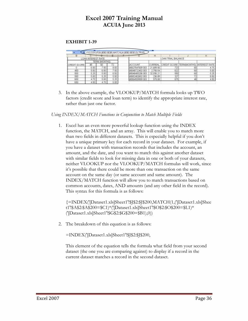
2. Type formula as follows: =VLOOKUP(lookup_value,table_array, MATCH(lookup_value,lookup_array,match_type),range_lookup; see Exhibit 1-39 for example)


Excel 2007 Page 36

EXHIBIT 1-39

3. In the above example, the VLOOKUP/MATCH formula looks up TWO factors (credit score and loan term) to identify the appropriate interest rate, rather than just one factor.

Using INDEX/MATCH Functions in Conjunction to Match Multiple Fields

1. Excel has an even more powerful lookup function using the INDEX

function, the MATCH, and an array. This will enable you to match more than two fields in different datasets. This is especially helpful if you don‘t have a unique primary key for each record in your dataset. For example, if you have a dataset with transaction records that includes the account, an amount, and the date, and you want to match this against another dataset with similar fields to look for missing data in one or both of your datasets, neither VLOOKUP nor the VLOOKUP/MATCH formulas will work, since it‘s possible that there could be more than one transaction on the same account on the same day (or same account and same amount). The INDEX/MATCH function will allow you to match transactions based on common accounts, dates, AND amounts (and any other field in the record). This syntax for this formula is as follows: {=INDEX('[Dataset1.xls]Sheet1'!$J$2:$J$200,MATCH(1,('[Dataset1.xls]Sheet1'!$A$2:$A$200=$C1)*('[Dataset1.xls]Sheet1'!$O$2:$O$200=$L1)* ('[Dataset1.xls]Sheet1'!$G$2:$G$200=$B1),0))

2. The breakdown of this equation is as follows: =INDEX('[Dataset1.xls]Sheet1'!$J$2:$J$200, This element of the equation tells the formula what field from your second dataset (the one you are comparing against) to display if a record in the current dataset matches a record in the second dataset.


Excel 2007 Page 37

3. MATCH(1, This tells Excel to look for all results totaling 1. It means that all the elements of the array portion that follows must return a ‗1‘, or the records will not match and it will return an ―#N/A‖ result.

4. ('[Dataset1.xls]Sheet1'!$A$2:$A$200=$C1) This element of the equation matches a field in the current dataset (in this case, the field in column C) with the first field in the second dataset (in this case, the field in column A). A match in this field returns a ‗1‘, an non-match returns a ‗0‘.

5. *('[Dataset1.xls]Sheet1'!$O$2:$O$200=$L1) This element of the equation matches a field in the current dataset (in this case, the field in column L) with a field in the second dataset (in this case, the field in column O). A match in this field returns a ‗1‘, an non-match returns a ‗0‘.

6. * ('[Dataset1.xls]Sheet1'!$G$2:$G$200=$B1) This element of the equation matches a field in the current dataset (in this case, the field in column B) with a field in the second dataset (in this case, the field in column G). A match in this field returns a ‗1‘, an non-match returns a ‗0‘.

7. Once you have typed in your formula, you MUST type

CTRL+SHIFT+ENTER, or the array portion of the formula WILL NOT work. You will know it works if Excel places a ―{‖ in front of the equal sign. Please note, it will not work to simply type the ―{‖ character; you must strike those three keys at the same time.

Working With Macros

Enabling Developer Ribbon

1. In order to create or record macros, you must first enable the Developer Ribbon. If this option has not already been enabled in your worksheet, open ‗Excel Options‘ screen (refer back to Exhibit 1-28).

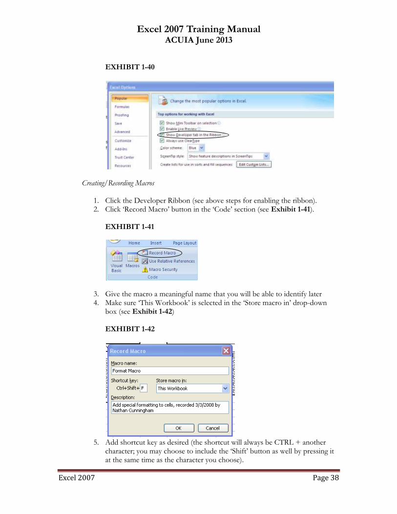
2. Ensure the ‗Popular‘ button is selected (see Exhibit 1-40). Click the ‗Show Developer tab in the Ribbon‘ option under ‗Top options for working with Excel‘.


Excel 2007 Page 38

EXHIBIT 1-40

Creating/Recording Macros

1. Click the Developer Ribbon (see above steps for enabling the ribbon). 2. Click ‗Record Macro‘ button in the ‗Code‘ section (see Exhibit 1-41).

EXHIBIT 1-41

3. Give the macro a meaningful name that you will be able to identify later 4. Make sure ‗This Workbook‘ is selected in the ‗Store macro in‘ drop-down

box (see Exhibit 1-42) EXHIBIT 1-42

5. Add shortcut key as desired (the shortcut will always be CTRL + another

character; you may choose to include the ‗Shift‘ button as well by pressing it at the same time as the character you choose).


Excel 2007 Page 39

6. Click ‗OK‘ (the macro will now start recording, think of it as a microphone recording every sound you make; from the time you click ‗OK‘ to the time you press the ‗Stop‘ button on the ‗Macro‘ toolbar, Excel will track your every keystroke for inclusion in the macro. So be careful and make sure you do not click or type anything you don‘t want in the macro!).

7. Click ‗Relative Reference‘ button on ‗Macro‘ toolbar to toggle relative cell references and absolute cell references (default is absolute; see Exhibit 1-43). EXHIBIT 1-43

8. Click ‗Stop‘ button to end macro recording. Accessing Recorded Macros

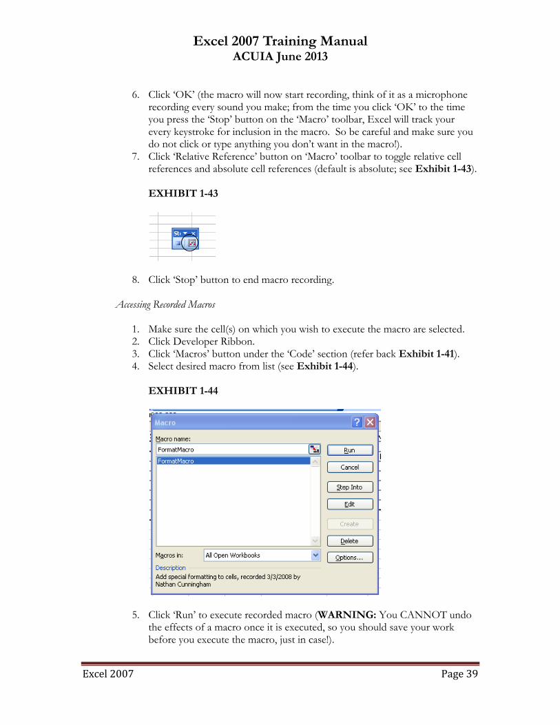
1. Make sure the cell(s) on which you wish to execute the macro are selected. 2. Click Developer Ribbon. 3. Click ‗Macros‘ button under the ‗Code‘ section (refer back Exhibit 1-41). 4. Select desired macro from list (see Exhibit 1-44).

EXHIBIT 1-44

5. Click ‗Run‘ to execute recorded macro (WARNING: You CANNOT undo the effects of a macro once it is executed, so you should save your work before you execute the macro, just in case!).


Excel 2007 Page 40

6. Click ‗Edit‘ to edit recorded macro (this will open Visual Basic editor; edit at your own risk!); you must select this option if you wish to change the name of the macro (you can also access the Visual Basic editor by either 1) selecting the appropriate button on under the ‗Code‘ section on the Developer Ribbon, refer back to Exhibit 1-41; or use the shortcut key ALT + F11).

7. Click ‗Step Into‘ to walk through the macro, step-by-step (this will also open Visual Basic editor; click F8 to advance to next line in the code).

8. Click ‗Options‘ to change the description or shortcut key for the macro. 9. Click ‗Delete‘ to remove macro.

Adding Macro Buttons to Quick Access Toolbar

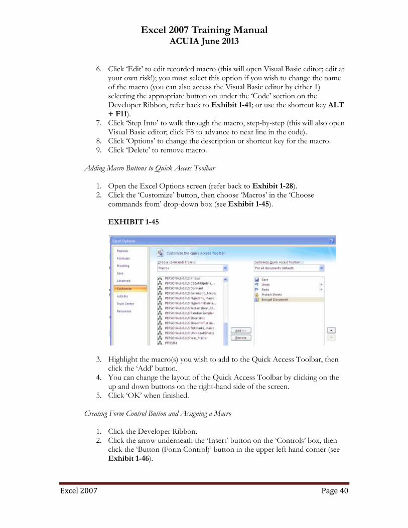
1. Open the Excel Options screen (refer back to Exhibit 1-28). 2. Click the ‗Customize‘ button, then choose ‗Macros‘ in the ‗Choose

commands from‘ drop-down box (see Exhibit 1-45). EXHIBIT 1-45

3. Highlight the macro(s) you wish to add to the Quick Access Toolbar, then click the ‗Add‘ button.

4. You can change the layout of the Quick Access Toolbar by clicking on the up and down buttons on the right-hand side of the screen.

5. Click ‗OK‘ when finished.

Creating Form Control Button and Assigning a Macro

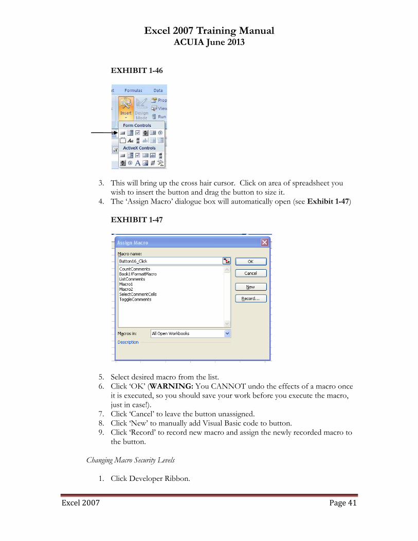
1. Click the Developer Ribbon. 2. Click the arrow underneath the ‗Insert‘ button on the ‗Controls‘ box, then

click the ‗Button (Form Control)‘ button in the upper left hand corner (see Exhibit 1-46).


Excel 2007 Page 41

EXHIBIT 1-46

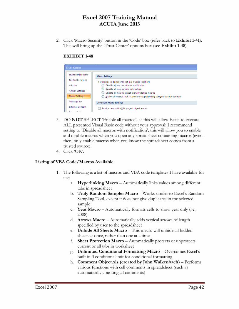
3. This will bring up the cross hair cursor. Click on area of spreadsheet you wish to insert the button and drag the button to size it.

4. The ‗Assign Macro‘ dialogue box will automatically open (see Exhibit 1-47) EXHIBIT 1-47

5. Select desired macro from the list. 6. Click ‗OK‘ (WARNING: You CANNOT undo the effects of a macro once

it is executed, so you should save your work before you execute the macro, just in case!).

7. Click ‗Cancel‘ to leave the button unassigned. 8. Click ‗New‘ to manually add Visual Basic code to button. 9. Click ‗Record‘ to record new macro and assign the newly recorded macro to

the button. Changing Macro Security Levels

1. Click Developer Ribbon.


Excel 2007 Page 42

2. Click ‗Macro Security‘ button in the ‗Code‘ box (refer back to Exhibit 1-41). This will bring up the ‗Trust Center‘ options box (see Exhibit 1-48). EXHIBIT 1-48

3. DO NOT SELECT ‗Enable all macros‘, as this will allow Excel to execute ALL presented Visual Basic code without your approval; I recommend setting to ‗Disable all macros with notification‘, this will allow you to enable and disable macros when you open any spreadsheet containing macros (even then, only enable macros when you know the spreadsheet comes from a trusted source).

4. Click ‗OK‘.

Listing of VBA Code/Macros Available

1. The following is a list of macros and VBA code templates I have available for use:

a. Hyperlinking Macro – Automatically links values among different tabs in spreadsheet

b. Truly Random Sampler Macro – Works similar to Excel‘s Random Sampling Tool, except it does not give duplicates in the selected sample

c. Year Macro – Automatically formats cells to show year only (i.e., 2008)

d. Arrows Macro – Automatically adds vertical arrows of length specified by user to the spreadsheet

e. Unhide All Sheets Macro – This macro will unhide all hidden sheets at once, rather than one at a time

f. Sheet Protection Macro – Automatically protects or unprotects current or all tabs in worksheet

g. Unlimited Conditional Formatting Macro – Overcomes Excel‘s built-in 3 conditions limit for conditional formatting

h. Comment Object.xls (created by John Walkenbach) – Performs various functions with cell comments in spreadsheet (such as automatically counting all comments)


Excel 2007 Page 43

i. Better Sheet Sorter.xls (created by John Walkenbach) – Automatically sorts all spreadsheets in workbook in alphabetical order

j. Delete Empty Rows.xls (created by John Walkenbach) – Automatically deletes all empty rows in a worksheet

k. Toggles.xls (created by John Walkenbach) – Toggles various cell formatting options (wrap text, headings, gridlines)

l. Add New Menu.xls (created by John Walkenbach) – Provides demonstration code for adding new menu to Excel

m. Loan Amortization Wizard.xla (created by John Walkenbach) – Excel Add-In that automatically generates a loan amortization schedule based on terms of user input

n. Export Import.xls (created by John Walkenbach) – Automatically exports or imports data to or from .CSV file

2. Others are available upon request Utilizing Formula Auditing Toolbar

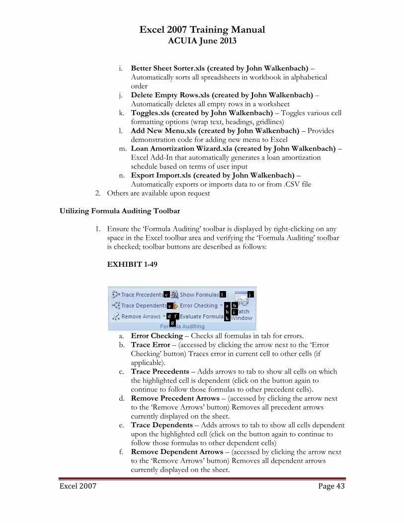
1. Ensure the ‗Formula Auditing‘ toolbar is displayed by right-clicking on any space in the Excel toolbar area and verifying the ‗Formula Auditing‘ toolbar is checked; toolbar buttons are described as follows: EXHIBIT 1-49

a. Error Checking – Checks all formulas in tab for errors. b. Trace Error – (accessed by clicking the arrow next to the ‗Error

Checking‘ button) Traces error in current cell to other cells (if applicable).

c. Trace Precedents – Adds arrows to tab to show all cells on which the highlighted cell is dependent (click on the button again to continue to follow those formulas to other precedent cells).

d. Remove Precedent Arrows – (accessed by clicking the arrow next to the ‗Remove Arrows‘ button) Removes all precedent arrows currently displayed on the sheet.

e. Trace Dependents – Adds arrows to tab to show all cells dependent upon the highlighted cell (click on the button again to continue to follow those formulas to other dependent cells)

f. Remove Dependent Arrows – (accessed by clicking the arrow next to the ‗Remove Arrows‘ button) Removes all dependent arrows currently displayed on the sheet.

h

g f

e

d

c

b a

i

j

k

l


Excel 2007 Page 44

g. Remove All Arrows – (accessed by clicking the arrow next to the ‗Remove Arrows‘ button) Removes all precedent and dependent arrows currently displayed on the sheet.

h. Circle Invalid Data – (accessed by clicking the arrow next to the ‗Error Checking‘ button; only available when circular references exist) Circles all cells with invalid data (i.e., circular references).

i. Clear Validation Circles – (accessed by clicking the arrow next to the ‗Error Checking‘ button; only available when circular references exist) Clears all circles currently displayed on sheet.

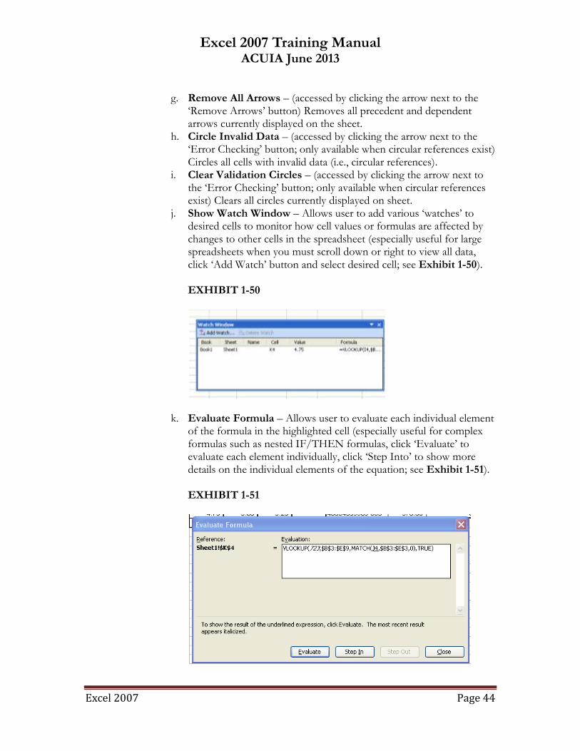
j. Show Watch Window – Allows user to add various ‗watches‘ to desired cells to monitor how cell values or formulas are affected by changes to other cells in the spreadsheet (especially useful for large spreadsheets when you must scroll down or right to view all data, click ‗Add Watch‘ button and select desired cell; see Exhibit 1-50). EXHIBIT 1-50

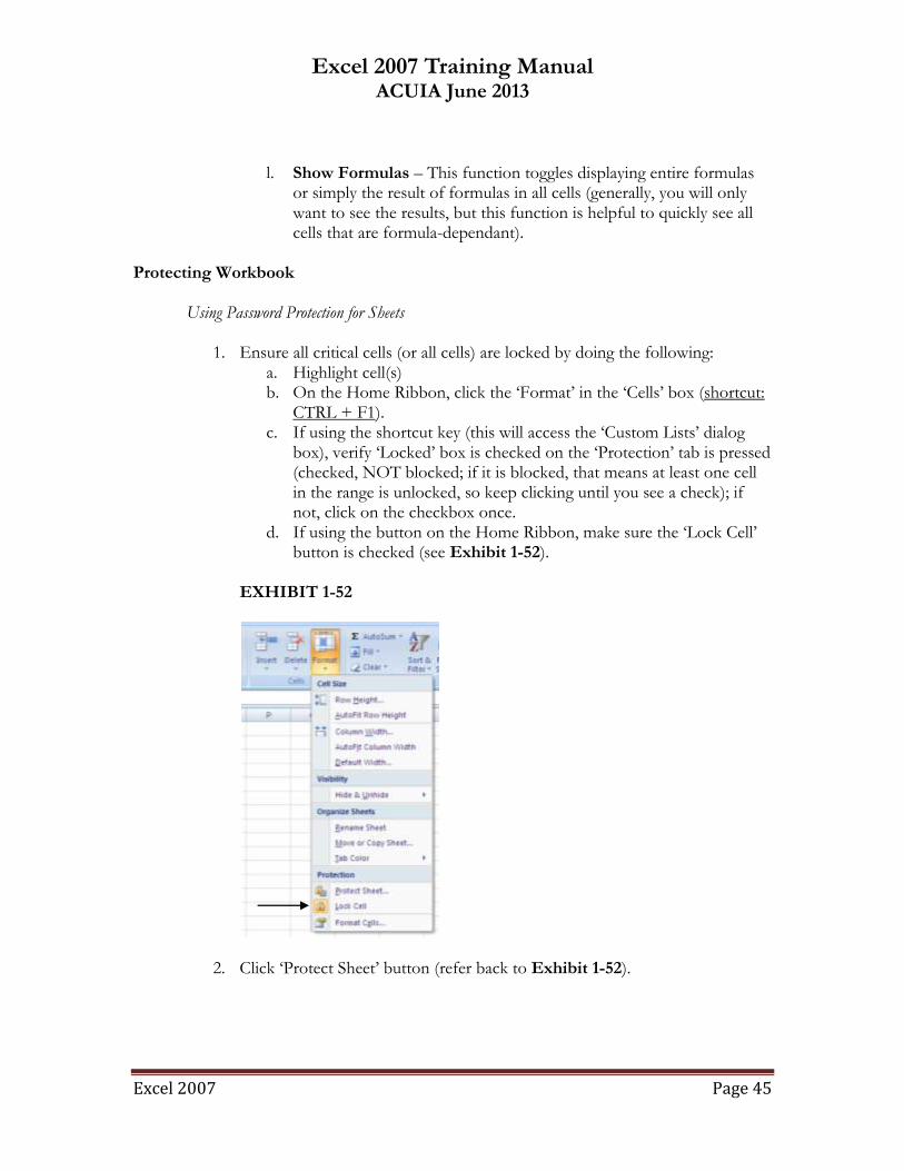
k. Evaluate Formula – Allows user to evaluate each individual element of the formula in the highlighted cell (especially useful for complex formulas such as nested IF/THEN formulas, click ‗Evaluate‘ to evaluate each element individually, click ‗Step Into‘ to show more details on the individual elements of the equation; see Exhibit 1-51). EXHIBIT 1-51


Excel 2007 Page 45

l. Show Formulas – This function toggles displaying entire formulas

or simply the result of formulas in all cells (generally, you will only want to see the results, but this function is helpful to quickly see all cells that are formula-dependant).

Protecting Workbook

Using Password Protection for Sheets

1. Ensure all critical cells (or all cells) are locked by doing the following: a. Highlight cell(s) b. On the Home Ribbon, click the ‗Format‘ in the ‗Cells‘ box (shortcut:

CTRL + F1). c. If using the shortcut key (this will access the ‗Custom Lists‘ dialog

box), verify ‗Locked‘ box is checked on the ‗Protection‘ tab is pressed (checked, NOT blocked; if it is blocked, that means at least one cell in the range is unlocked, so keep clicking until you see a check); if not, click on the checkbox once.

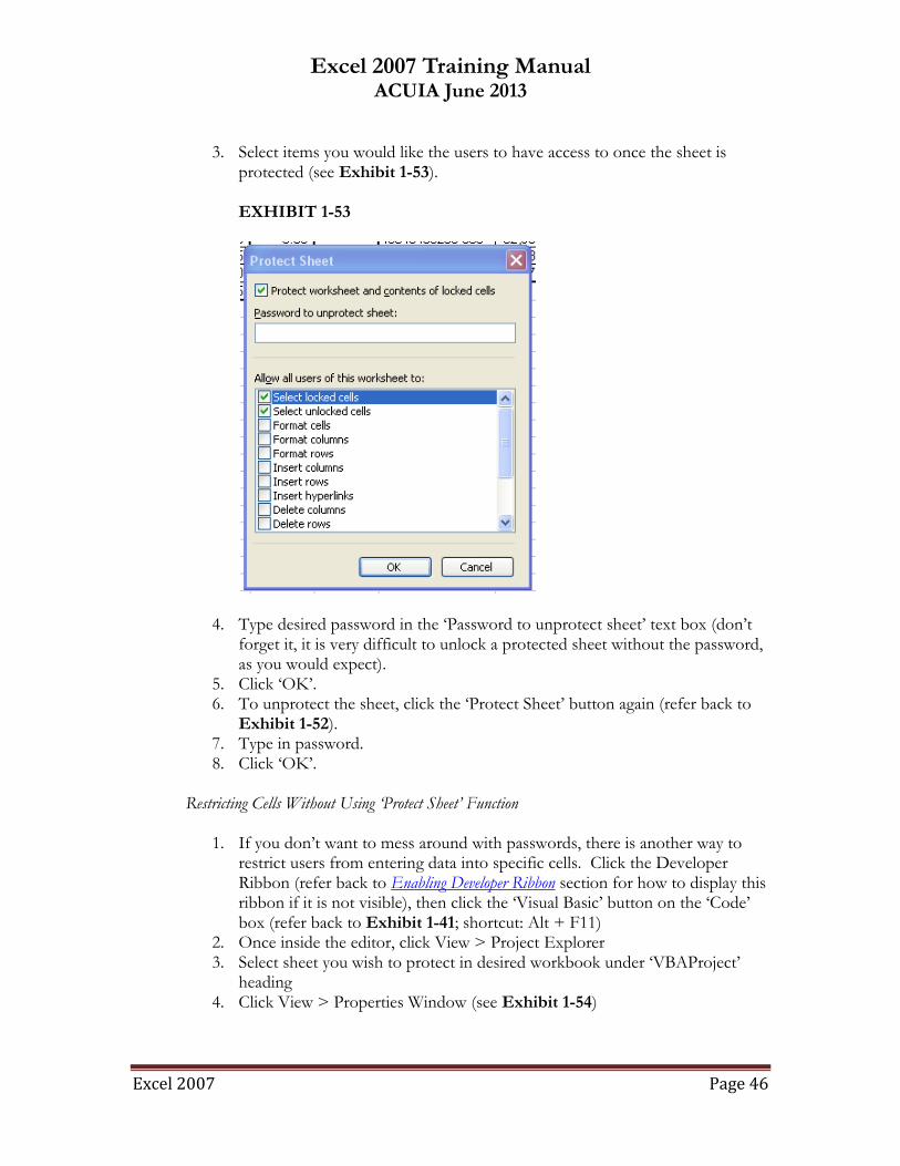
d. If using the button on the Home Ribbon, make sure the ‗Lock Cell‘ button is checked (see Exhibit 1-52).

EXHIBIT 1-52

2. Click ‗Protect Sheet‘ button (refer back to Exhibit 1-52).


Excel 2007 Page 46

3. Select items you would like the users to have access to once the sheet is protected (see Exhibit 1-53). EXHIBIT 1-53

4. Type desired password in the ‗Password to unprotect sheet‘ text box (don‘t forget it, it is very difficult to unlock a protected sheet without the password, as you would expect).

5. Click ‗OK‘. 6. To unprotect the sheet, click the ‗Protect Sheet‘ button again (refer back to

Exhibit 1-52). 7. Type in password. 8. Click ‗OK‘.

Restricting Cells Without Using ‘Protect Sheet’ Function

1. If you don‘t want to mess around with passwords, there is another way to

restrict users from entering data into specific cells. Click the Developer Ribbon (refer back to Enabling Developer Ribbon section for how to display this ribbon if it is not visible), then click the ‗Visual Basic‘ button on the ‗Code‘ box (refer back to Exhibit 1-41; shortcut: Alt + F11)

2. Once inside the editor, click View > Project Explorer 3. Select sheet you wish to protect in desired workbook under ‗VBAProject‘

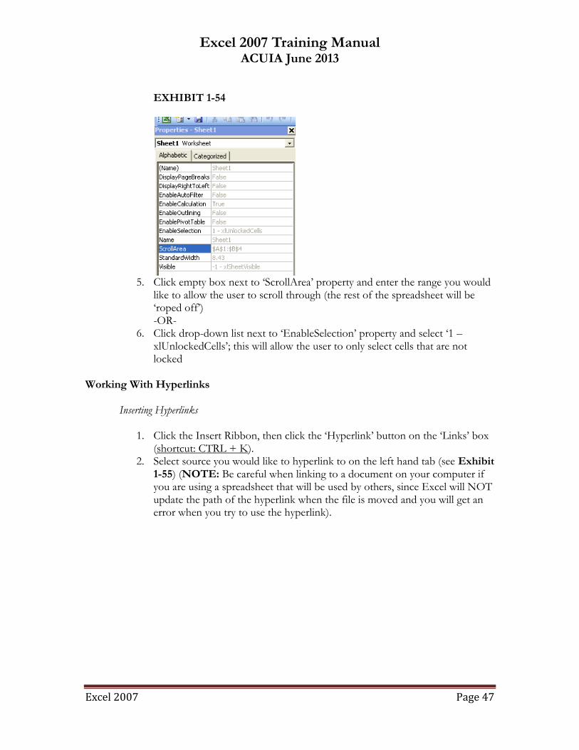
heading 4. Click View > Properties Window (see Exhibit 1-54)


Excel 2007 Page 47

EXHIBIT 1-54

5. Click empty box next to ‗ScrollArea‘ property and enter the range you would

like to allow the user to scroll through (the rest of the spreadsheet will be ‗roped off‘) -OR-

6. Click drop-down list next to ‗EnableSelection‘ property and select ‗1 – xlUnlockedCells‘; this will allow the user to only select cells that are not locked

Working With Hyperlinks

Inserting Hyperlinks

1. Click the Insert Ribbon, then click the ‗Hyperlink‘ button on the ‗Links‘ box (shortcut: CTRL + K).

2. Select source you would like to hyperlink to on the left hand tab (see Exhibit 1-55) (NOTE: Be careful when linking to a document on your computer if you are using a spreadsheet that will be used by others, since Excel will NOT update the path of the hyperlink when the file is moved and you will get an error when you try to use the hyperlink).


Excel 2007 Page 48

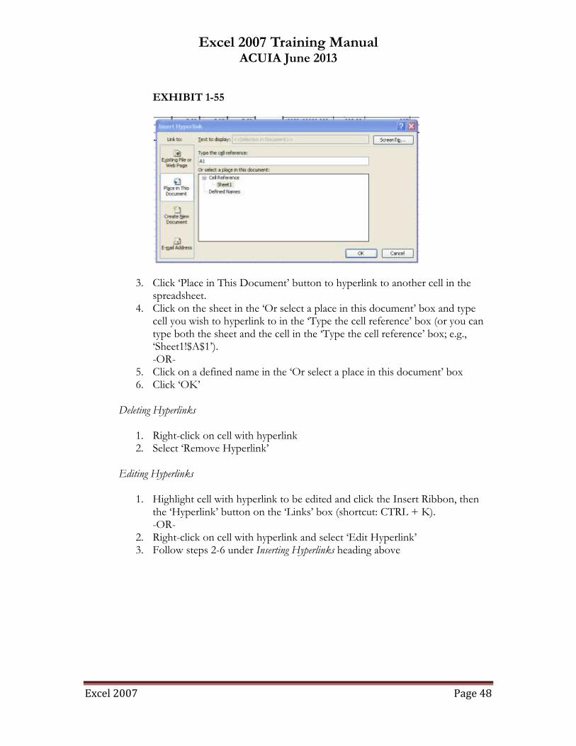
EXHIBIT 1-55

3. Click ‗Place in This Document‘ button to hyperlink to another cell in the spreadsheet.

4. Click on the sheet in the ‗Or select a place in this document‘ box and type cell you wish to hyperlink to in the ‗Type the cell reference‘ box (or you can type both the sheet and the cell in the ‗Type the cell reference‘ box; e.g., ‗Sheet1!$A$1‘). -OR-

5. Click on a defined name in the ‗Or select a place in this document‘ box 6. Click ‗OK‘

Deleting Hyperlinks

1. Right-click on cell with hyperlink 2. Select ‗Remove Hyperlink‘

Editing Hyperlinks

1. Highlight cell with hyperlink to be edited and click the Insert Ribbon, then

the ‗Hyperlink‘ button on the ‗Links‘ box (shortcut: CTRL + K). -OR-

2. Right-click on cell with hyperlink and select ‗Edit Hyperlink‘ 3. Follow steps 2-6 under Inserting Hyperlinks heading above


Excel 2007 Page 49

SUMPRODUCT and SUMIFS Formulas

1. Excel has a formula array that allows the user to determine if an item meets multiple criteria, and will count or sum the items that meet the multiple criteria. To access this function, follow the instructions from step 3 on in the Inserting Function section above, or simply type ‗=sumproduct(‘ to access the formula tool tip.

2. In this example, if I had a loan trail balance and wanted to find out the sum of all loans with a balance in excess of $20,000 and at least 30 days overdue, I would add elements of the formula are as follows: =SUMPRODUCT(($C$2:$C$43>20000)*($E$2:$E$43>=30)*($C$2:$C$43)) The first two elements are the criteria. The third element is tells the formula to return the sum of the loans meeting the first two criteria. If I left the third element out, the formula would return the count of loans meeting the first two criteria (NOTE: While this can be used as an array formula, you do not have to use the CTRL+SHIFT+ENTER keystroke for it to work properly). I can add as many criteria as I wish (up to 127) to qualify my results.

3. Excel‘s SUMIFS function works similarly. To return the same result from the SUMPRODUCT example above, I would add elements to the formula as follows: =SUMIFS($C$2:$C$43,$C$2:$C$43,">20000",$E$2:$E$43,">=30") The first element is the range to be summed, the next element is the range of the first criteria, the third element is the first criteria, the fourth element is the range of the second criteria, and the final element is the second criteria. Please note that the first element must ALWAYS be the summed range.

4. There are a few differences between SUMIFS and SUMPRODUCT. a. For one, it is not as flexible (as described above, SUMPRODUCT

can function as both a COUNTIFS function and a SUMIFS function).

b. Also, SUMPRODUCT works better with date search qualifiers [e.g. YEAR(), MONTH()]. Going back to the previous example, suppose I wanted to add an additional criteria to show loans originated during 2009. While this is possible for both formulas, the SUMPRODUCT is easier to construct, as follows: =SUMPRODUCT(($C$2:$C$43>20000)*($E$2:$E$43>=30)*($C$2:$C$43)*(YEAR($D$2:$D$43)=2009)) To return the same result for the SUMIFS formula, you would have to use this equation:


Excel 2007 Page 50

=SUMIFS($C$2:$C$43,$C$2:$C$43,">20000",$E$2:$E$43,">=30",$D$2:$D$43,">=01/01/2009",$D$2:$D$43,"<=12/31/2009") As you can see, SUMIFS requires two additional elements to return the same result.

c. Conversely, SUMIFS works better with wildcards than SUMPRODUCT does. Going back to the original example, suppose I wanted to find all loans with member names with a last name of ‗Young‘, in addition to the other criteria. The SUMIFS formula would look like this: =SUMIFS($C$2:$C$43,$C$2:$C$43,">20000",$E$2:$E$43,">=30",$B$2:$B$43,"*YOUNG*") With SUMPRODUCTS, I‘d have to ‗trick‘ Excel into using the search function as follows: =SUMPRODUCT(($C$2:$C$43>20000)*($E$2:$E$43>=30)*($C$2:$C$43)*(ISNUMBER(SEARCH("YOUNG",$B$2:$B$43))))

Both formulas are powerful for summarizing large amounts of data in whatever way you wish.

Calculating Loan Payment Streams with CUMPRINC and CUMINT

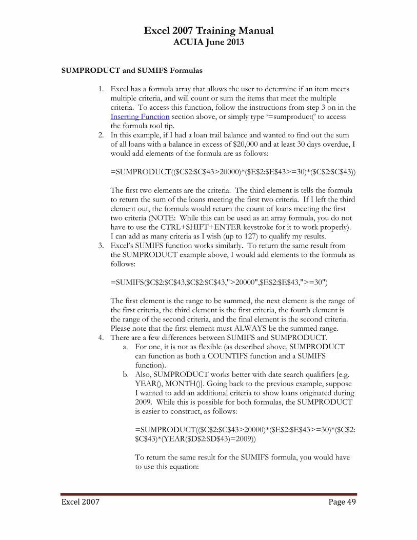
1. Excel has two powerful built-in formulas that will calculate either the amount of principal or the amount of interest for any range of payments in a constant loan payment stream. The easiest way to populate this formula is to type ‗=-CUMIPMT(‘ (or CUMPRINC if you wish to calculate principal), then click on the ‗Insert Function‘ button on the formula toolbar (see Exhibit 1-56).

EXHIBIT 1-56

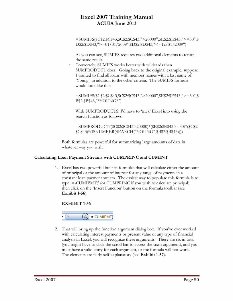
2. That will bring up the function argument dialog box. If you‘ve ever worked with calculating interest payments or present value or any type of financial analysis in Excel, you will recognize these arguments. There are six in total (you might have to click the scroll bar to access the sixth argument), and you must have a valid entry for each argument, or the formula will not work. The elements are fairly self-explanatory (see Exhibit 1-57).


Excel 2007 Page 51

EXHIBIT 1-57

3. A few tips…in general, you will need to divide the interest rate by the number of payments to be made per year (usually 12).

4. You can enter any number between 1 and the value of ‗Nper‘ (number of total periods for the loan; in this case, 180 months).

5. The sixth element is ‗Type‘. In general, this should be ‗0‘, meaning that payments are due at the end of the period (the other option is ‗1‘, meaning payments are due at the beginning of the period).

6. These formulas are useful for determining interest and principal over a specified period without creating a complete loan amortization schedule.


Excel 2007 Page 52

Performing Advanced Analysis in Excel

Linear (Two-Factor) Regression Analysis

1. Organize your data into rows and columns, with independent variables in on row or column and dependent variables in the other row or column (NOTE: Excel will assume the independent variables are on the left and will plot numbers on the ‗x‘ axis‘; see Exhibit 1-58 for example). EXHIBIT 1-58

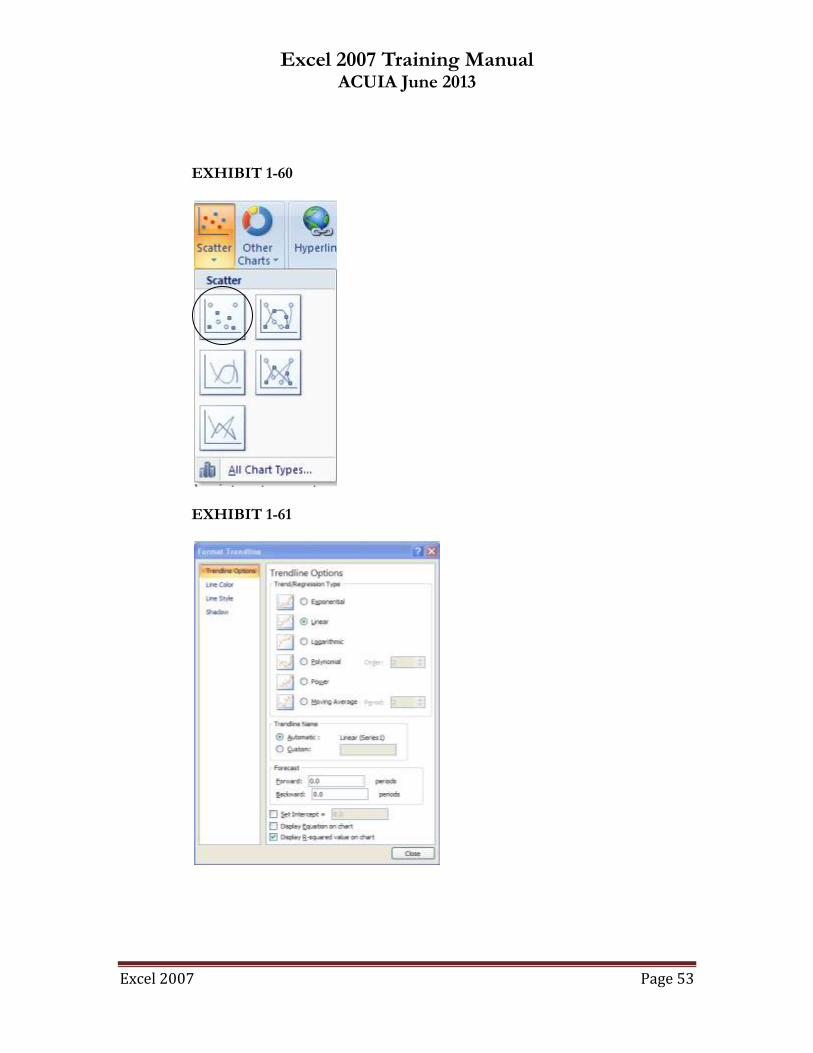
2. Highlight data, click ‗Insert‘ ribbon, then click ‗Scatter‘ button (see Exhibit 1-

59). This will provide a drop-down with several options; select ‗Scatter with only Markers‘ option, which is the top, left-hand option (see Exhibit 1-60). This should create a scatter graph chart.

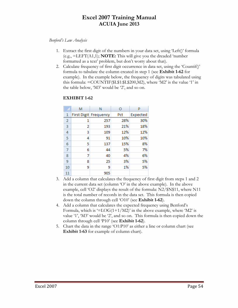
3. Add a trendline to the chart by selecting the data points on the chart, right-click, select ‗Add Trendline‘.

4. This should bring up the ‗Format Trendline‘ dialog box (see Exhibit 1-61). Make sure ‗Linear‘ is selected.

5. Check the ‗Display R-squared value on chart‘ box. EXHIBIT 1-59


Excel 2007 Page 53

EXHIBIT 1-60

EXHIBIT 1-61


Excel 2007 Page 54

Benford’s Law Analysis

1. Extract the first digit of the numbers in your data set, using ‗Left()‘ formula (e.g., =LEFT(A1,1); NOTE: This will give you the dreaded ‗number formatted as a text‘ problem, but don‘t worry about that).

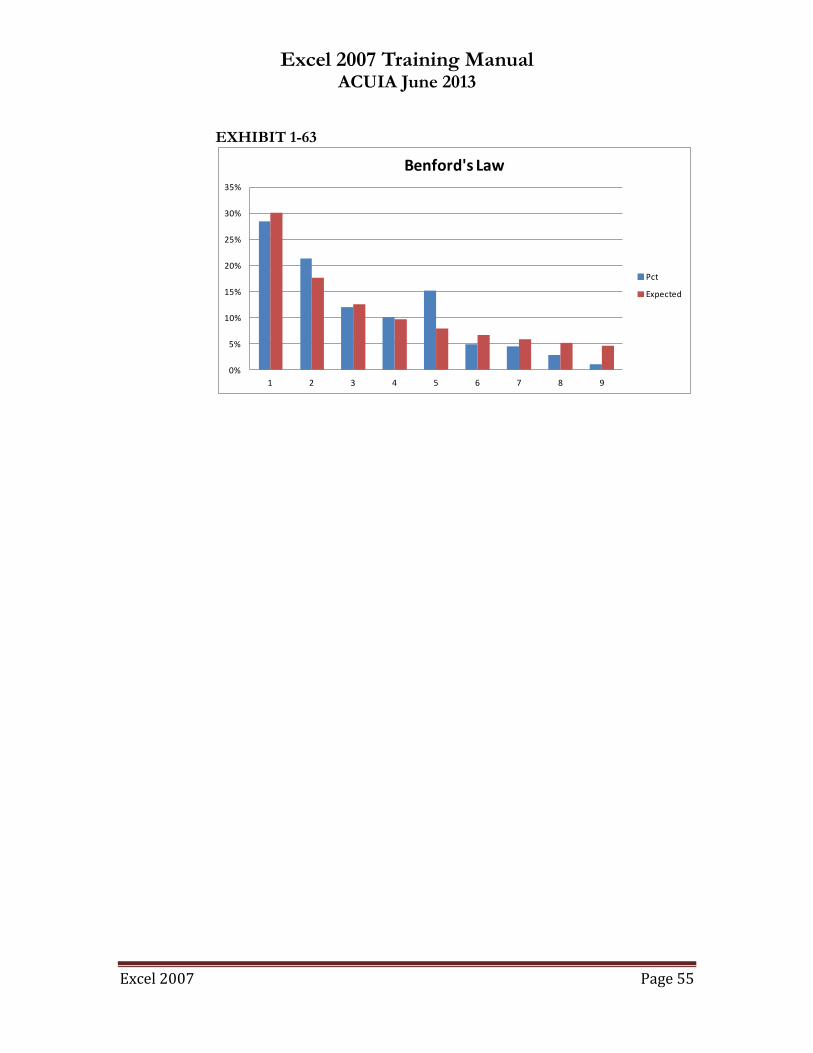
2. Calculate frequency of first digit occurrence in data set, using the ‗Countif()‘ formula to tabulate the column created in step 1 (see Exhibit 1-62 for example). In the example below, the frequency of digits was tabulated using this formula: =COUNTIF($L$1:$L$200,M2), where ‗M2‘ is the value ‗1‘ in the table below, ‗M3‘ would be ‗2‘, and so on. EXHIBIT 1-62

3. Add a column that calculates the frequency of first digit from steps 1 and 2

in the current data set (column ‗O‘ in the above example). In the above example, cell ‗O2‘ displays the result of the formula: N2/$N$11, where N11 is the total number of records in the data set. This formula is then copied down the column through cell ‗O10‘ (see Exhibit 1-62).

4. Add a column that calculates the expected frequency using Benford‘s Formula, which is ‗=LOG(1+1/M2)‘ in the above example, where ‗M2‘ is value ‗1‘, ‗M3‘ would be ‗2‘, and so on. This formula is then copied down the column through cell ‗P10‘ (see Exhibit 1-62).

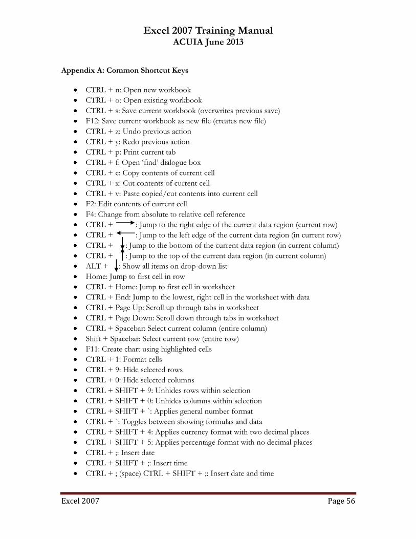
5. Chart the data in the range ‗O1:P10‘ as either a line or column chart (see Exhibit 1-63 for example of column chart).


Excel 2007 Page 55

EXHIBIT 1-63

0%

5%

10%

15%

20%

25%

30%

35%

1 2 3 4 5 6 7 8 9

Benford's Law

Pct

Expected


Excel 2007 Page 56

Appendix A: Common Shortcut Keys

CTRL + n: Open new workbook

CTRL + o: Open existing workbook

CTRL + s: Save current workbook (overwrites previous save)

F12: Save current workbook as new file (creates new file)

CTRL + z: Undo previous action

CTRL + y: Redo previous action

CTRL + p: Print current tab

CTRL + f: Open ‗find‘ dialogue box

CTRL + c: Copy contents of current cell

CTRL + x: Cut contents of current cell

CTRL + v: Paste copied/cut contents into current cell

F2: Edit contents of current cell

F4: Change from absolute to relative cell reference

CTRL + : Jump to the right edge of the current data region (current row)

CTRL + : Jump to the left edge of the current data region (in current row)

CTRL + : Jump to the bottom of the current data region (in current column)

CTRL + : Jump to the top of the current data region (in current column)

ALT + : Show all items on drop-down list

Home: Jump to first cell in row

CTRL + Home: Jump to first cell in worksheet

CTRL + End: Jump to the lowest, right cell in the worksheet with data

CTRL + Page Up: Scroll up through tabs in worksheet

CTRL + Page Down: Scroll down through tabs in worksheet

CTRL + Spacebar: Select current column (entire column)

Shift + Spacebar: Select current row (entire row)

F11: Create chart using highlighted cells

CTRL + 1: Format cells

CTRL + 9: Hide selected rows

CTRL + 0: Hide selected columns

CTRL + SHIFT + 9: Unhides rows within selection

CTRL + SHIFT + 0: Unhides columns within selection

CTRL + SHIFT + `: Applies general number format

CTRL + `: Toggles between showing formulas and data

CTRL + SHIFT + 4: Applies currency format with two decimal places

CTRL + SHIFT + 5: Applies percentage format with no decimal places

CTRL + ;: Insert date

CTRL + SHIFT + ;: Insert time

CTRL + ; (space) CTRL + SHIFT + ;: Insert date and time

Documents

Excel 2007 Training Manual - ACUIA.org - Excel Training...Excel 2007 Training Manual ... Excel 2007 Training Manual ACUIA June 2013 Excel 2007 Page 2 ... to the area labeled Report