1

EXCEL ADVANCED

2

Mathematical Operators for Excel

• <• >• =• >=• <=• <>• ^

• Less than• greater than• Equal• Greater than or equal• Less than or equal• Not equal• Power of

3

Functions

• SUMIFS• Adds the cells in a

range that meet multiple criteria

• COUNTIFS• Applies criteria to

cells across multiple ranges and counts the number of times all criteria are met

The key difference between these and Countif/Sumif is that these allow the use of multiple criteria. Countif/Sumif do not

4

Formulas/Functions cont.

• Can also use “FUNCTION WIZARD”

• =IF(Logical test,Value_if_true,Value_if_false)

• =PMT(rate/12,nper,pv)

• =FV(rate,nper,pmt,pv)– Returns the FUTURE value of an investment– Unless otherwise stated-the pmt is “0”– Do NOT have to divide INTEREST RATE by 12, or multiply NPER

by 12 (yrs.)

• =PV(rate,nper,pmt,fv)– Returns the PRESENT value of an investment– Unless otherwise stated-the pmt is “0”– Do NOT have to divide INTEREST RATE by 12, or multiply NPER

by 12 (yrs.)

5

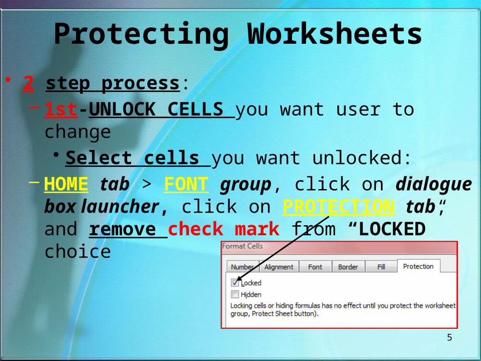
Protecting Worksheets

• 2 step process:– 1st-UNLOCK CELLS you want user to change

• Select cells you want unlocked:– HOME tab > FONT group, click on dialogue box

launcher, click on PROTECTION tab, and remove check mark from “LOCKED” choice

6

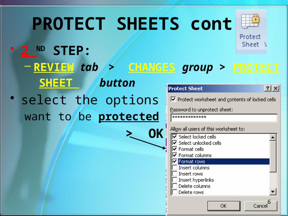
PROTECT SHEETS cont.• 2 ND STEP:

– REVIEW tab > CHANGES group > PROTECT

SHEET button• select the options you

want to be protected

> OK

7

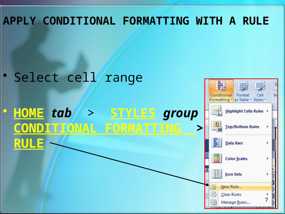
APPLY CONDITIONAL FORMATTING WITH A RULE

• Select cell range

• HOME tab > STYLES group > CONDITIONAL FORMATTING > NEW RULE

8

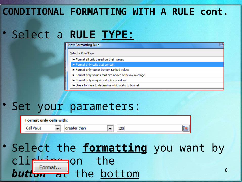
CONDITIONAL FORMATTING WITH A RULE cont.

• Select a RULE TYPE:

• Set your parameters:

• Select the formatting you want by clicking on the button at the bottom

9

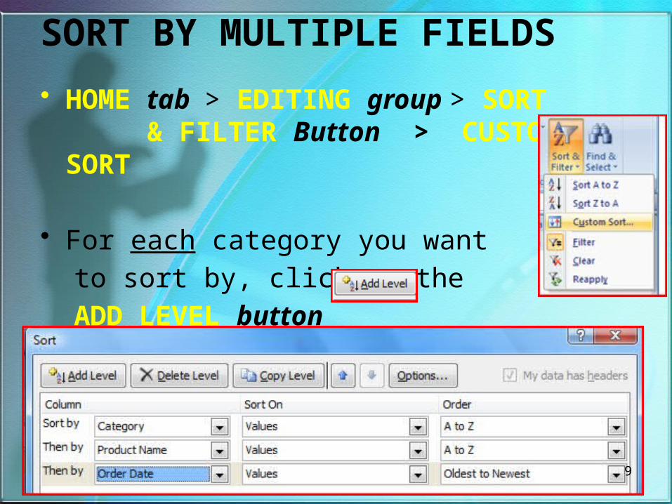
SORT BY MULTIPLE FIELDS

• HOME tab > EDITING group > SORT & FILTER Button > CUSTOM SORT

• For each category you want

to sort by, click on the

ADD LEVEL button

10

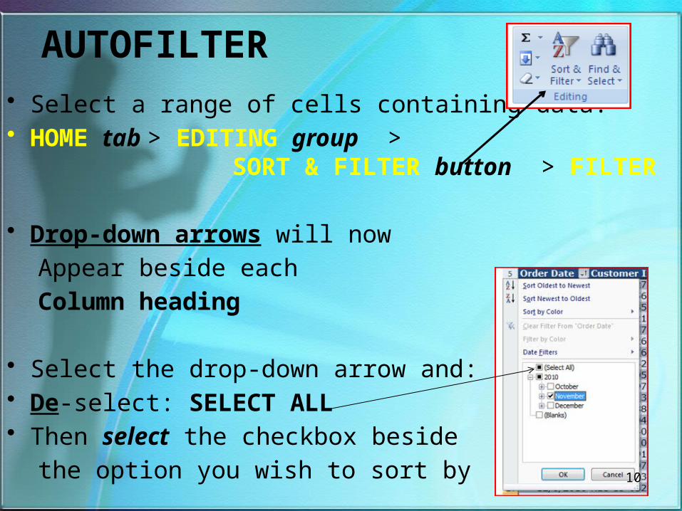
AUTOFILTER

• Select a range of cells containing data. • HOME tab > EDITING group >

SORT & FILTER button > FILTER

• Drop-down arrows will now

Appear beside each

Column heading

• Select the drop-down arrow and:• De-select: SELECT ALL• Then select the checkbox beside

the option you wish to sort by

11

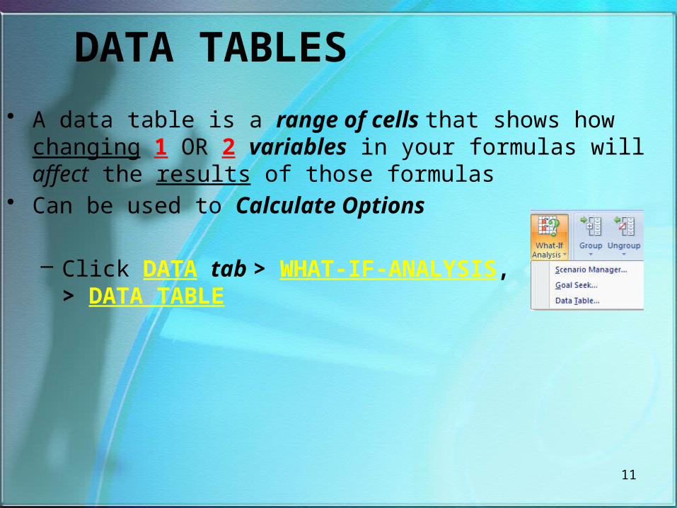
DATA TABLES

• A data table is a range of cells that shows how changing 1 OR 2 variables in your formulas will affect the results of those formulas

• Can be used to Calculate Options

– Click DATA tab > WHAT-IF-ANALYSIS,> DATA TABLE

12

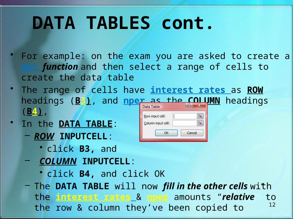
DATA TABLES cont.

• For example: on the exam you are asked to create a pmt function and then select a range of cells to create the data table

• The range of cells have interest rates as ROW headings (B3), and nper as the COLUMN headings (B4),

• In the DATA TABLE:– ROW INPUTCELL:

• click B3, and– COLUMN INPUTCELL:

• click B4, and click OK – The DATA TABLE will now fill in the other cells with the

interest rates & nper amounts “relative” to the row & column they’ve been copied to

13

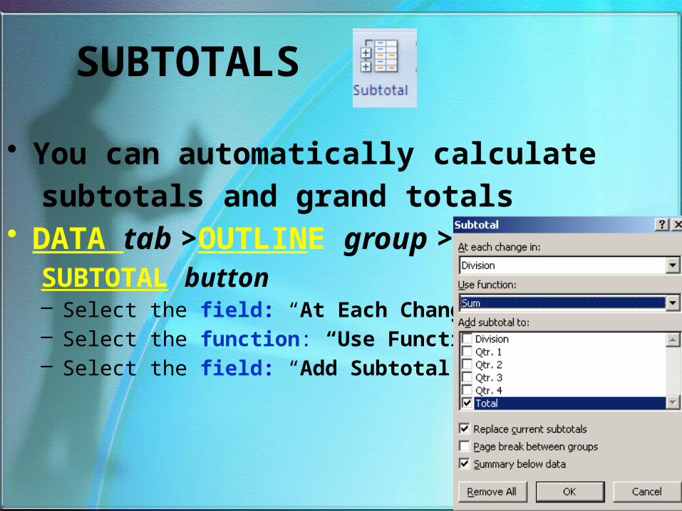
SUBTOTALS

• You can automatically calculate

subtotals and grand totals• DATA tab >OUTLINE group >

SUBTOTAL button– Select the field: “At Each Change In”– Select the function: “Use Function”– Select the field: “Add Subtotal to” > OK

14

PIVOT CHARTS• When you create a “regular” chart:

– You create 1 chart for each “view” of the data that you want to see

• When you create a “PIVOT” chart:– You also create a single chart BUT:

• You can view the data in different ways by changing the report :

– Layout OR– The detail displayed

15

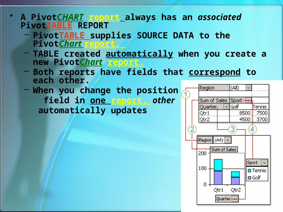
• A PivotCHART report always has an associated PivotTABLE REPORT – PivotTABLE supplies SOURCE DATA to the PivotChart

report. – TABLE created automatically when you create a new

PivotChart report.– Both reports have fields that correspond to each other. – When you change the position of a

field in one report, other report automatically updates

16

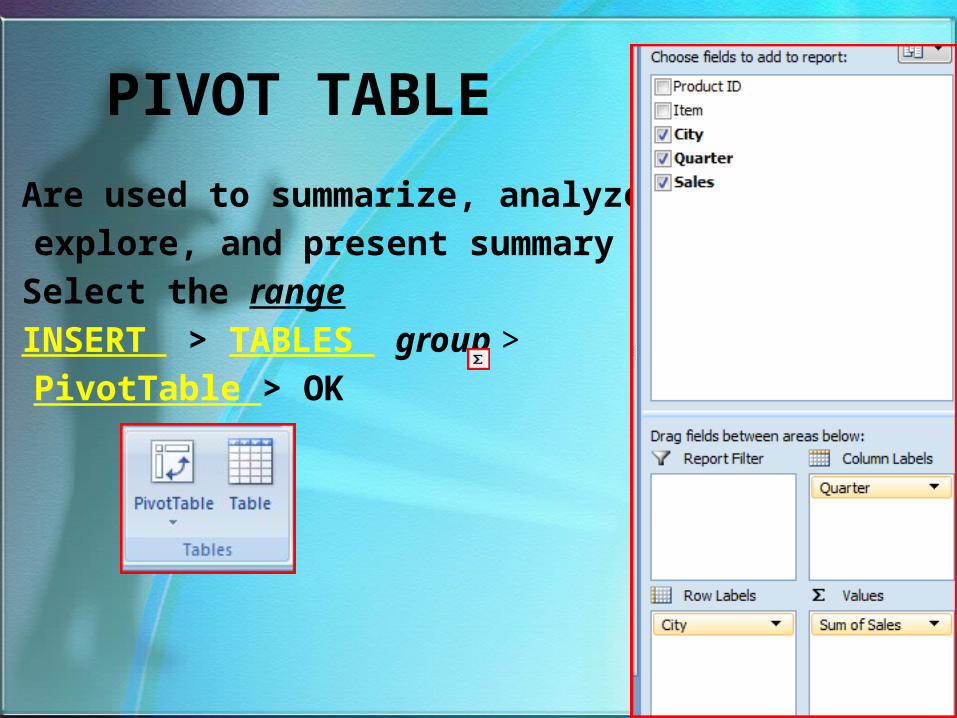
PIVOT TABLE

• Are used to summarize, analyze,

explore, and present summary data• Select the range• INSERT > TABLES group >

PivotTable > OK

17

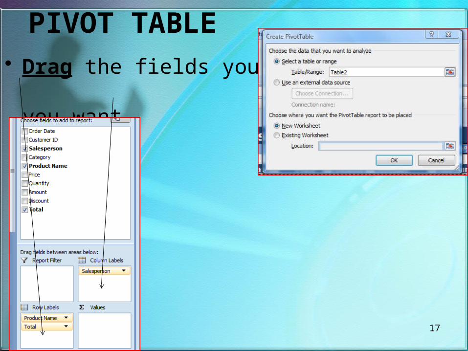
PIVOT TABLE• Drag the fields you want

into the areas you want

18

PIVOT TABLE cont.

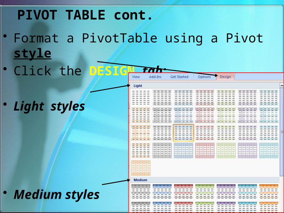
• Format a PivotTable using a Pivot style• Click the DESIGN tab:

• Light styles

• Medium styles

19

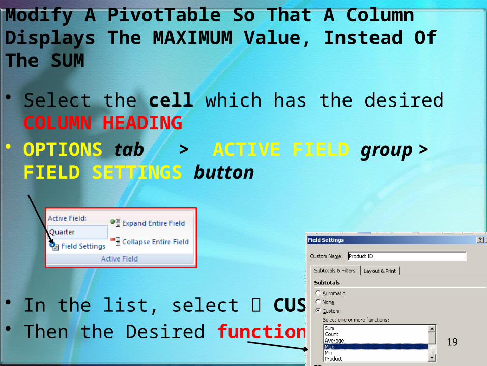
Modify A PivotTable So That A Column Displays The MAXIMUM Value, Instead Of The SUM

• Select the cell which has the desired COLUMN HEADING

• OPTIONS tab > ACTIVE FIELD group > FIELD SETTINGS button

• In the list, select CUSTOM• Then the Desired function > OK

20

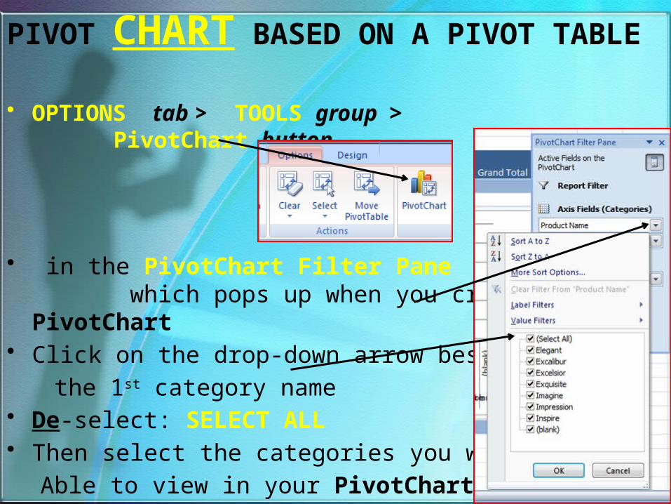
PIVOT CHART BASED ON A PIVOT TABLE

• OPTIONS tab > TOOLS group > PivotChart button

• in the PivotChart Filter Pane which pops up when you create the PivotChart

• Click on the drop-down arrow beside

the 1st category name• De-select: SELECT ALL• Then select the categories you want to be

Able to view in your PivotChart > OK

21

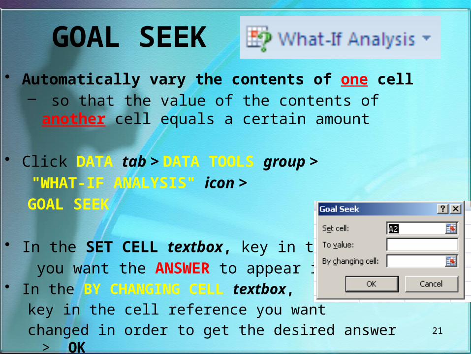
GOAL SEEK• Automatically vary the contents of one cell

– so that the value of the contents of another cell equals a certain amount

• Click DATA tab > DATA TOOLS group >

"WHAT-IF ANALYSIS" icon >

GOAL SEEK

• In the SET CELL textbox, key in the cell

you want the ANSWER to appear in• In the BY CHANGING CELL textbox,

key in the cell reference you want

changed in order to get the desired answer > OK

22

FREE “TIP OF THE WEEK”