Excel 2007 Tutorial

Tab 0 1 of 42 6/12/04

8/16/2009PREFACE TO EXCEL TUTORIAL Excel is essential when analyzing finance cases. Most students have taken a course that covers the basics of Excel, including accessing the program, adding and subtracting, copying, and the like. Although some students are quite proficient, most need help when dealing advanced features, and this Tutorial provides that help. Procedurally, we developed a series of cases on financial management, wrote models to analyze them, tested the cases and models in our classes, and identified the Excel features that caused students trouble. We then wrote this tutorial to help clarify the trouble spots.1

We recommend that you skim through the tutorial, get an idea of what it covers, and then use it as a reference as you go through the cases. The models provide references to the Tutorial at the point where advanced Excel features are used. For example, all of the case models use Data Table to do sensitivity analysis. If you are not familiar with Data Tables, when you first encounter them in a model go to the tutorial for instructions on how to make and use them. Many Excel features are used repeatedly in the cases, so taking the time to learn them in the early cases will make the later cases easier. Excel is useful for things other than working finance cases, so what you learn about Excel will benefit you in other courses and in the real world after you graduate. Indeed, recruiters tell us that students who are proficient with Excel have a definite advantage in the job market, and our former students tell us that having Excel skills is a big help in moving up the ladder. So, learning more about Excel is well worth the effort!

1 If students need more help than the Tutorial provides, we recommend Mayes and Shank, Financial Analysis With Microsoft Excel, 5th ed. (South-Western Cengage Learning, 2009).

Tab 1. Contents 2 of 42 6/12/04

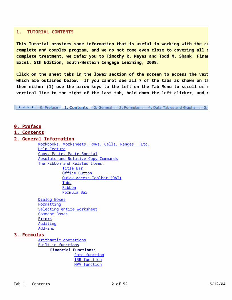
0. Preface1. Contents

2. General InformationWorkbooks, Worksheets, Rows, Cells, Ranges, Etc.Help FeatureCopy, Paste, Paste SpecialAbsolute and Relative Copy CommandsThe Ribbon and Related Items:

Title BarOffice ButtonQuick Access Toolbar (QAT)TabsRibbonFormula Bar

Dialog BoxesFormattingSelecting entire worksheetComment BoxesErrorsAuditingAdd-ins

3. FormulasArithmetic operationsBuilt-in functions

Financial Functions:Rate functionIRR functionNPV function

1. TUTORIAL CONTENTS

This Tutorial provides some information that is useful in working with the case models. Excel is a very complete and complex program, and we do not come even close to covering all of its features. For a more complete treatment, we refer you to Timothy R. Mayes and Todd M. Shank, Financial Analysis With Microsoft Excel, 5th Edition, South-Western Cengage Learning, 2009.

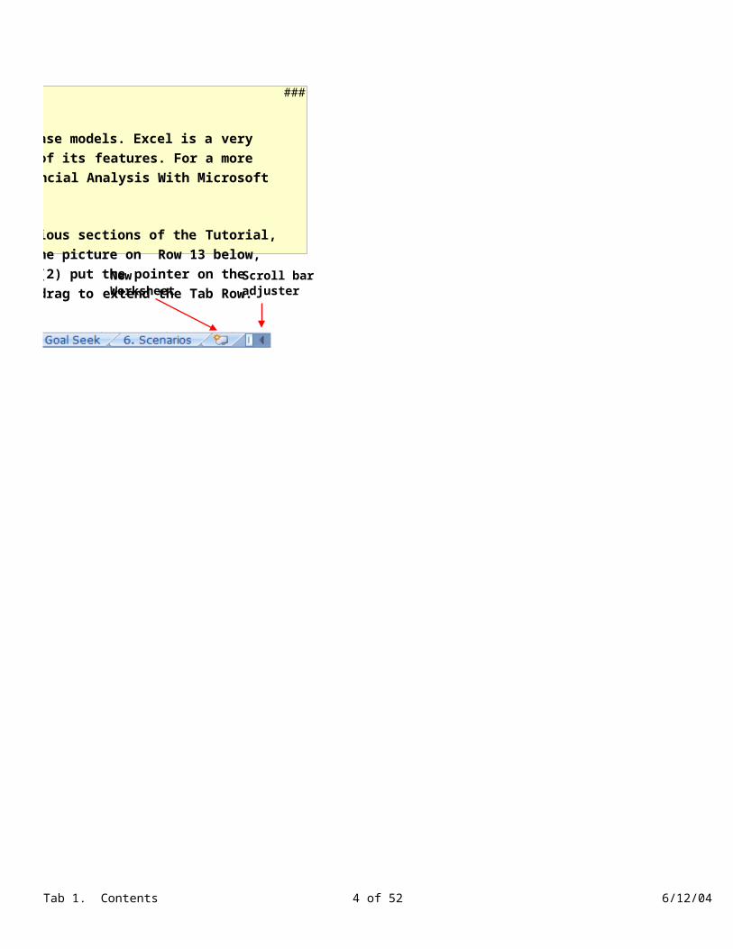
Click on the sheet tabs in the lower section of the screen to access the various sections of the Tutorial, which are outlined below. If you cannot see all 7 of the tabs as shown on the picture on Row 13 below, then either (1) use the arrow keys to the left on the Tab Menu to scroll or (2) put the pointer on the vertical line to the right of the last tab, hold down the left clicker, and drag to extend the Tab Row.


PV functionDate functions (need for bonds)Bond Price and Yield functions

PRICE functionYIELD functionAccrued Interest

Other finance functions

Statistical Functions:LOGEST functionSLOPE functionSTDEV functionSTDEVP functionOther Statistical functions

Math and Trig functions

Logical functions: IF

RegressionSimple (1 independent variable)Multiple (2 or more variables)

4. Data Tables, Sorting, and GraphsData functions

Data Tables: 1 Input, 1 OutputData Tables: 1 Input, 2 OutputsData Tables: 2 Inputs, 1 Output

Sorting DataGraphs

5. Goal Seek

6. Scenario Analysis


8/16/2009

New Scroll bar Worksheet adjuster

1. TUTORIAL CONTENTS

This Tutorial provides some information that is useful in working with the case models. Excel is a very complete and complex program, and we do not come even close to covering all of its features. For a more complete treatment, we refer you to Timothy R. Mayes and Todd M. Shank, Financial Analysis With Microsoft Excel, 5th Edition, South-Western Cengage Learning, 2009.

Click on the sheet tabs in the lower section of the screen to access the various sections of the Tutorial, which are outlined below. If you cannot see all 7 of the tabs as shown on the picture on Row 13 below, then either (1) use the arrow keys to the left on the Tab Menu to scroll or (2) put the pointer on the vertical line to the right of the last tab, hold down the left clicker, and drag to extend the Tab Row.

Tab 2. General Information 5 of 42 6/12/04

I. Workbooks, Worksheets, Rows, Columns, Cells, and Ranges

Sheet Tabs

HELP

2. GENERAL INFORMATION We repeat here our caveat -- we cannot in this Tutorial tell you about all the features and quirks in Excel. We explain some, but you will encounter more as you work with Excel. Again, we recommend the Mayes-Shank book.

This file, like all Excel files, is called a Workbook. Workbooks contain one or more Worksheets. Our current file is named "Excel 2007 Tutorial." It is a workbook that consists of 7 worksheets. You are now on the worksheet called "2. General." You can move from worksheet to worksheet by clicking on the tabs at the bottom of the screen. If there are many worksheets, some tabs may be hidden. To see them, click on the arrows to the left of the tabs and scroll to the item of interest.

There are 1,048,756 rows and 16,384 columns, hence 17,182,818,304 cells on each worksheet. The columns are designated A, B, …, XFD, and the rows are numbered from 1 to 1048756. Therefore, the cells go from A1 to XFD1048756. Normally, you will only use a small fraction of the cells available on the "Big Grid."

It is difficult to navigate through a huge worksheet. Therefore, we typically break workbooks into sections and place different sections on different worksheets, tabbing to go between them.

If you have information on one worksheet--say input data--that you want to process on another worksheet, you can transfer it automatically. In the cell where you want to use the data, click the equal sign, then tab to the worksheet with the input data (or formula), select the appropriate cell, click the enter key, and the data will be transferred to where you want it.

A set of adjacent cells is called a range, and you can give it a name. Then, whenever you want to refer to the set of cells, you can call up the range by its name. You can learn more about this and all the other items discussed in this Tutorial from Excel's Help feature as discussed below.

In the models, we generally use bright blue to indicate model inputs, dark blue for general discussion, black type for formulas, and yellow shading for answers. We use other colors randomly for contrast and to liven up the worksheets.

As noted above, workbooks can have several worksheets, each accessed by a sheet tab. Normally, new workbooks show three tabs, named Sheet 1, Sheet 2, and Sheet 3. You can right click on a tab and then delete it, change its name, or move it. Also, you can left click and then drag tabs so as to rearrange their order on the tab row, and you can use the arrows to scroll if there are many tabs on the worksheet. You can add worksheets by clicking the Insert Worksheet button after the last sheet tab.

Excel's Help feature is tremendously useful, and you should experiment with it as you go through this Tutorial and as you work with the models. Click the Help button in the upper-right corner of the application window. Then type in a word or words describing what you want information about, and then click the most appropriate item in the list that appears. For example, type in the word "copy" and then click Search. You will then be given a list of topics related to copying. Click on the one you think is most appropriate and then follow the instructions. Some experimentation is often necessary to learn how to do various things, but you should eventually attain your goal.


Copy, Cut, Paste, and Paste Special

Absolute and Relative Copy Commands

The Ribbon

Office Button Quick Access Toolbar (QAT)

Tabs

You can highlight selected cells and then copy the information (leaving it in the original cell) to another cell. Highlight the cell to be copied, click the copy button, put the pointer on the cell where the information is to go, and click the paste button. You could also move the information by clicking the cut button rather than the copy button.

If you copy a cell and the information in the cell later changes, the new information is also reflected in the cell to which the copy was made. That is sometimes, but not always, desirable. If you do not want the information to change, you can use the paste special feature. Click the copy icon, put the pointer on the target cell, then click Edit, click paste special, check the box labeled values, and then click OK. The copied data will then not change even if the original cell changes. We use this feature in a number of the case models, where we do scenario analysis.

If you copy cells with values (numbers), the information is transmitted exactly to the new cell. However, if you copy formulas, the cell references may be copied exactly or be shifted. Exact copies are designated "absolute" and to get this, you must put $ signs in front of the column and row designators. Without the $ signs, we are making a "relative" copy, and the cell references change. You can get the $ signs by typing them in or by selecting the cell with the formula and then clicking the F4 key, once to set both the row and column to absolute values, and then repeated clicks can be used to make only the row or column absolute.

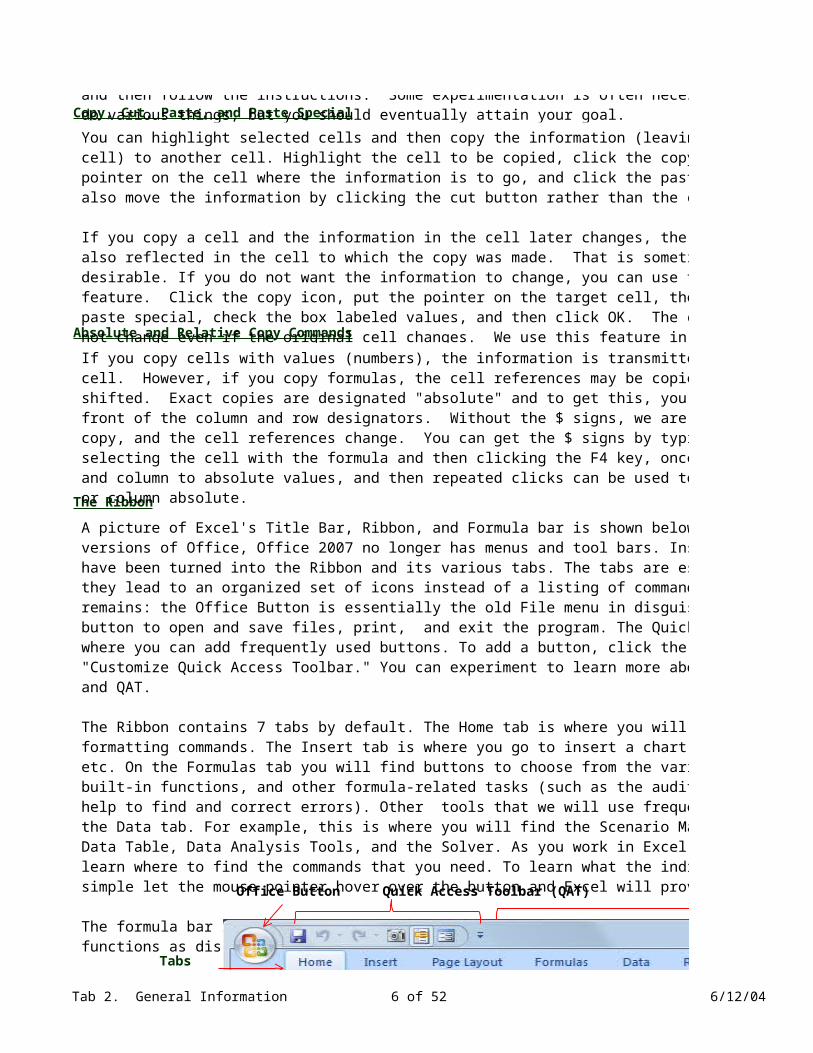
A picture of Excel's Title Bar, Ribbon, and Formula bar is shown below. Unlike previous versions of Office, Office 2007 no longer has menus and tool bars. Instead, the old menus have been turned into the Ribbon and its various tabs. The tabs are essentially menus, but they lead to an organized set of icons instead of a listing of commands. Only one menu remains: the Office Button is essentially the old File menu in disguise. Click the Office button to open and save files, print, and exit the program. The Quick Access Toolbar is where you can add frequently used buttons. To add a button, click the QAT and choose "Customize Quick Access Toolbar." You can experiment to learn more about the Office Button and QAT.

The Ribbon contains 7 tabs by default. The Home tab is where you will find common formatting commands. The Insert tab is where you go to insert a chart, shape, Pivot Table, etc. On the Formulas tab you will find buttons to choose from the various categories of built-in functions, and other formula-related tasks (such as the auditing tools, which help to find and correct errors). Other tools that we will use frequently can be found on the Data tab. For example, this is where you will find the Scenario Manager, Goal Seek, Data Table, Data Analysis Tools, and the Solver. As you work in Excel you will quickly learn where to find the commands that you need. To learn what the individual buttons do, simple let the mouse pointer hover over the button and Excel will provide a description.

The formula bar is where you do arithmetic and also use Excel's very important built-in functions as discussed below.


The Ribbon

Formula Bar

Dialog Boxes

Formatting

Selecting the entire worksheet

When we use different Ribbon features in the case models, we refer to the tabs, groups, and icons where the commands can be found.

When you click on certain icons, you open a dialog box, where you provide Excel with additional information needed to complete an operation. We illustrate dialog boxes in the Formulas worksheet.

You can select a cell or range of cells and then format the data by clicking on one or more of the buttons on the Home tab. For example, you can use the increase decimal button (in the Number group) to set the number of decimal places displayed. You can make text bold or underlined by clicking the appropriate button the the Font group of the Home tab. Other buttons allow you to use color fill in the background, change the font face, add borders, or change the alignment of text in a cell.

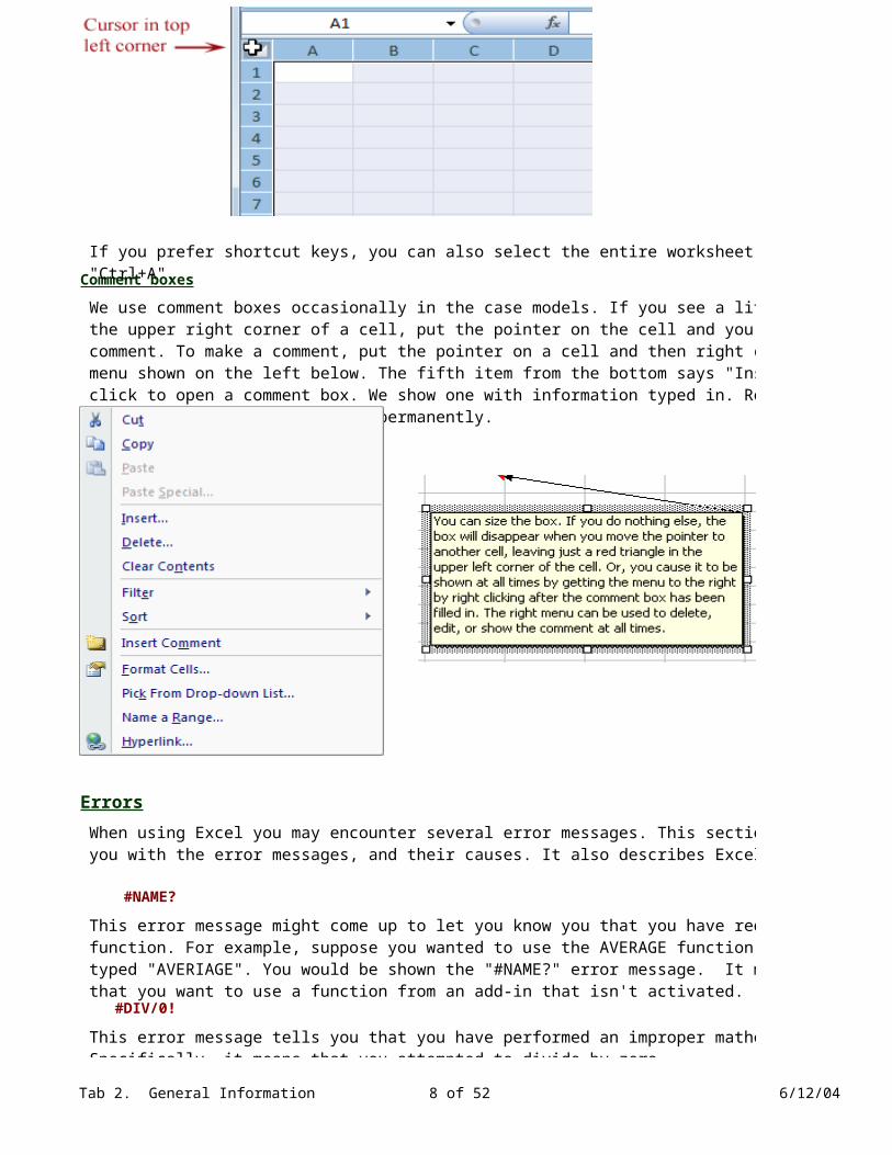
Some formatting options are not available on the Home tab. For these, you can select a range and then right click and choose Format Cells from the shortcut menu. You can experiment with this at your convenience, using Help as necessary. Note particularly that you can hide rows, columns, or cells. To unhide them, go back into Format and click unhide. We generally click in the upper left corner of the worksheet to highlight the entire worksheet (see below) before doing the unhide operation.

Also, you might note that we use Format Cells to make subscripts, superscripts, underlines, and the like in text such as you are now reading. Not only can you format cells, but you can format portions of text with cells. You simply have to highlight the portion of text you wish to format and then proceed in the Format menu. You can subscript, superscript, underline, and much more.

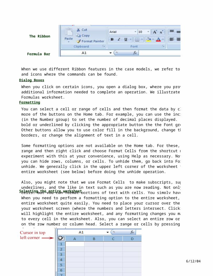
When you need to perform a formatting option to the entire worksheet, you can select the entire worksheet quite easily. You need to place your cursor over the top left section of your worksheet screen (where the numbers and letters intersect. Clicking on this "cell" will highlight the entire worksheet, and any formatting changes you make will be applied to every cell in the worksheet. Also, you can select an entire row or column by clicking on the row number or column head. Select a range or cells by pressing left click and dragging over the chosen range.


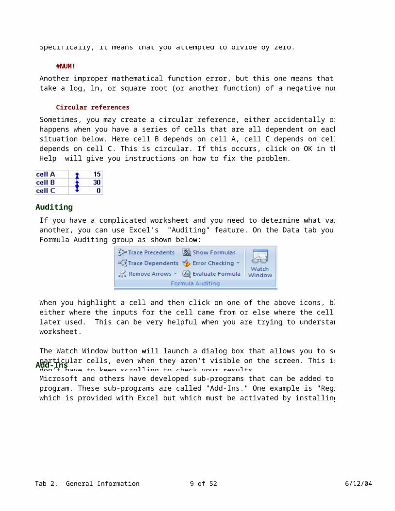
Comment boxes

Errors

#NAME?

#DIV/0!

If you prefer shortcut keys, you can also select the entire worksheet by pressing "Ctrl+A".

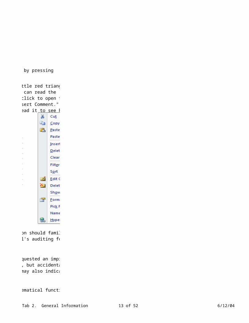
We use comment boxes occasionally in the case models. If you see a little red triangle in the upper right corner of a cell, put the pointer on the cell and you can read the comment. To make a comment, put the pointer on a cell and then right click to open the menu shown on the left below. The fifth item from the bottom says "Insert Comment." Left click to open a comment box. We show one with information typed in. Read it to see how to delete, edit, or show the box permanently.

When using Excel you may encounter several error messages. This section should familiarize you with the error messages, and their causes. It also describes Excel's auditing feature.

This error message might come up to let you know you that you have requested an improper function. For example, suppose you wanted to use the AVERAGE function, but accidentally typed "AVERIAGE". You would be shown the "#NAME?" error message. It may also indicate that you want to use a function from an add-in that isn't activated.

This error message tells you that you have performed an improper mathematical function. Specifically, it means that you attempted to divide by zero.


#NUM!

Circular references

Auditing

Add-Ins

Another improper mathematical function error, but this one means that you attempted to take a log, ln, or square root (or another function) of a negative number.

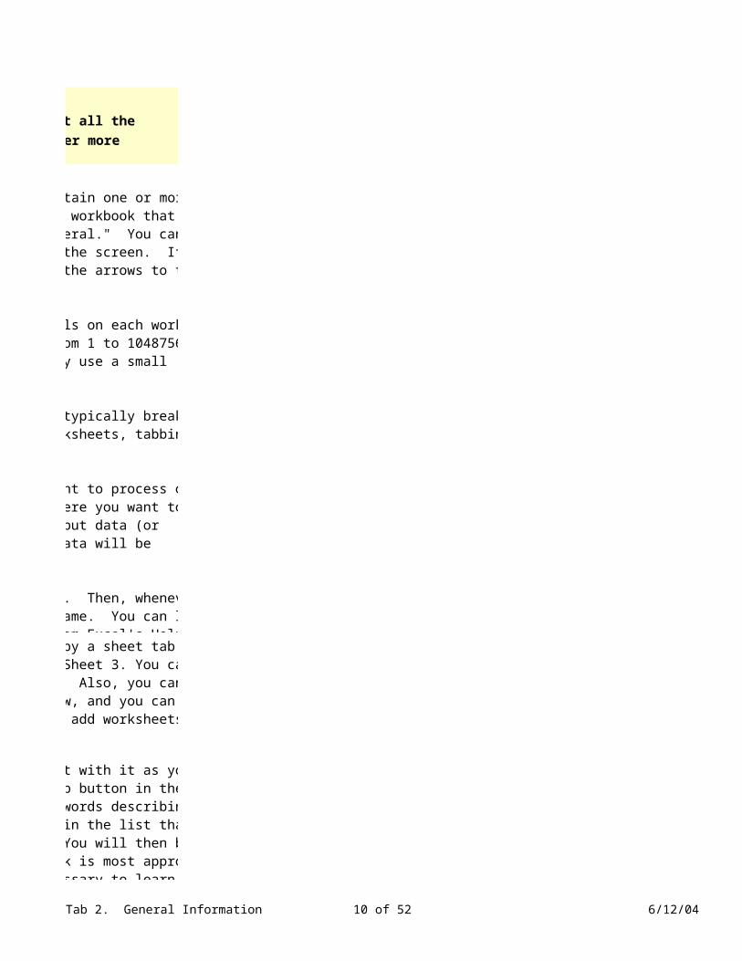
Sometimes, you may create a circular reference, either accidentally or by design. This happens when you have a series of cells that are all dependent on each other, such as the situation below. Here cell B depends on cell A, cell C depends on cell B, and cell A depends on cell C. This is circular. If this occurs, click on OK in the error message and Help will give you instructions on how to fix the problem.

If you have a complicated worksheet and you need to determine what variables depend on one another, you can use Excel's "Auditing" feature. On the Data tab you will find the Formula Auditing group as shown below:

When you highlight a cell and then click on one of the above icons, blue arrows will show either where the inputs for the cell came from or else where the cell's information is later used. This can be very helpful when you are trying to understand a complicated worksheet.

The Watch Window button will launch a dialog box that allows you to see information about particular cells, even when they aren't visible on the screen. This is useful so that you don't have to keep scrolling to check your results.

Microsoft and others have developed sub-programs that can be added to the basic Excel program. These sub-programs are called "Add-Ins." One example is "Regression Analysis," which is provided with Excel but which must be activated by installing it to the program. See Tab 3, Row 306, for instructions on activating the Analysis ToolPak add-in. This Add-In provides a collection of statistical analysis tools, including regression analysis.

You will need to have this Add-In installed to do many of the cases, so you might as well install it now. Click the Office Button and then the Excel Options button in the lower right corner. In the dialog box, click Add-ins on the left side, and then click the Go button at the bottom. Finally, place a check mark next to "Analysis ToolPak" to load the add-in. It will now be available every time you start Excel. Note that you do not need to enable the "Analysis ToolPak - VBA" add-in unless you plan to use the functions in VBA code.

Tab 3. Formulas 10 of 42 6/12/04

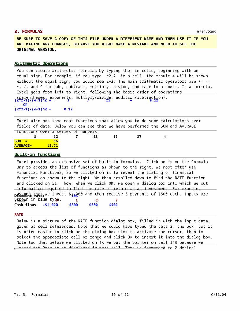
3. FORMULAS 8/16/2009

Arithmetic Operations

(2*2-1)/(4+1)^2 = 3 / 25 = 0.12---OR---

(2*2-1)/(4+1)^2 = 0.12

8 12 7 23 15 27 4SUM = 96AVERAGE= 13.71

Built-in functions

Discount rate: 10%Years 0 1 2 3Cash flows -$1,000 $500 $500 $500

RATE

BE SURE TO SAVE A COPY OF THIS FILE UNDER A DIFFERENT NAME AND THEN USE IT IF YOU ARE MAKING ANY CHANGES, BECAUSE YOU MIGHT MAKE A MISTAKE AND NEED TO SEE THE ORIGINAL VERSION.

You can create arithmetic formulas by typing them in cells, beginning with an equal sign. For example, if you type =2+2 in a cell, the result 4 will be shown. Without the equal sign, you would see 2+2. The main arithmetic operators are +, -, *, /, and ^ for add, subtract, multiply, divide, and take to a power. In a formula, Excel goes from left to right, following the basic order of operations (parentheses; exponents; multiply/divide; addition/subtraction).

Excel also has some neat functions that allow you to do some calculations over fields of data. Below you can see that we have performed the SUM and AVERAGE functions over a series of numbers.

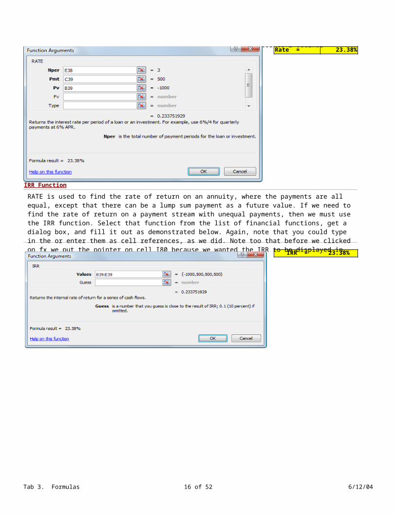
Excel provides an extensive set of built-in formulas. Click on fx on the Formula Bar to access the list of functions as shown to the right. We most often use Financial Functions, so we clicked on it to reveal the listing of financial functions as shown to the right. We then scrolled down to find the RATE function and clicked on it. Now, when we click OK, we open a dialog box into which we put information required to find the rate of return on an investment. For example, assume that we invest $1,000 and then receive 3 payments of $500 each. Inputs are shown in blue type.

Below is a picture of the RATE function dialog box, filled in with the input data, given as cell references. Note that we could have typed the data in the box, but it is often easier to click on the dialog box slot to activate the cursor, then to select the appropriate cell or range and click OK to insert it into the dialog box. Note too that before we clicked on fx we put the pointer on cell I49 because we wanted the Rate to be displayed in that cell. Then we formatted to 2 decimal places, highlighted, and boxed the answer.


Rate = 23.38%

IRR Function

IRR = 23.38%

RATE is used to find the rate of return on an annuity, where the payments are all equal, except that there can be a lump sum payment as a future value. If we need to find the rate of return on a payment stream with unequal payments, then we must use the IRR function. Select that function from the list of financial functions, get a dialog box, and fill it out as demonstrated below. Again, note that you could type in the or enter them as cell references, as we did. Note too that before we clicked on fx we put the pointer on cell I80 because we wanted the IRR to be displayed in that cell.


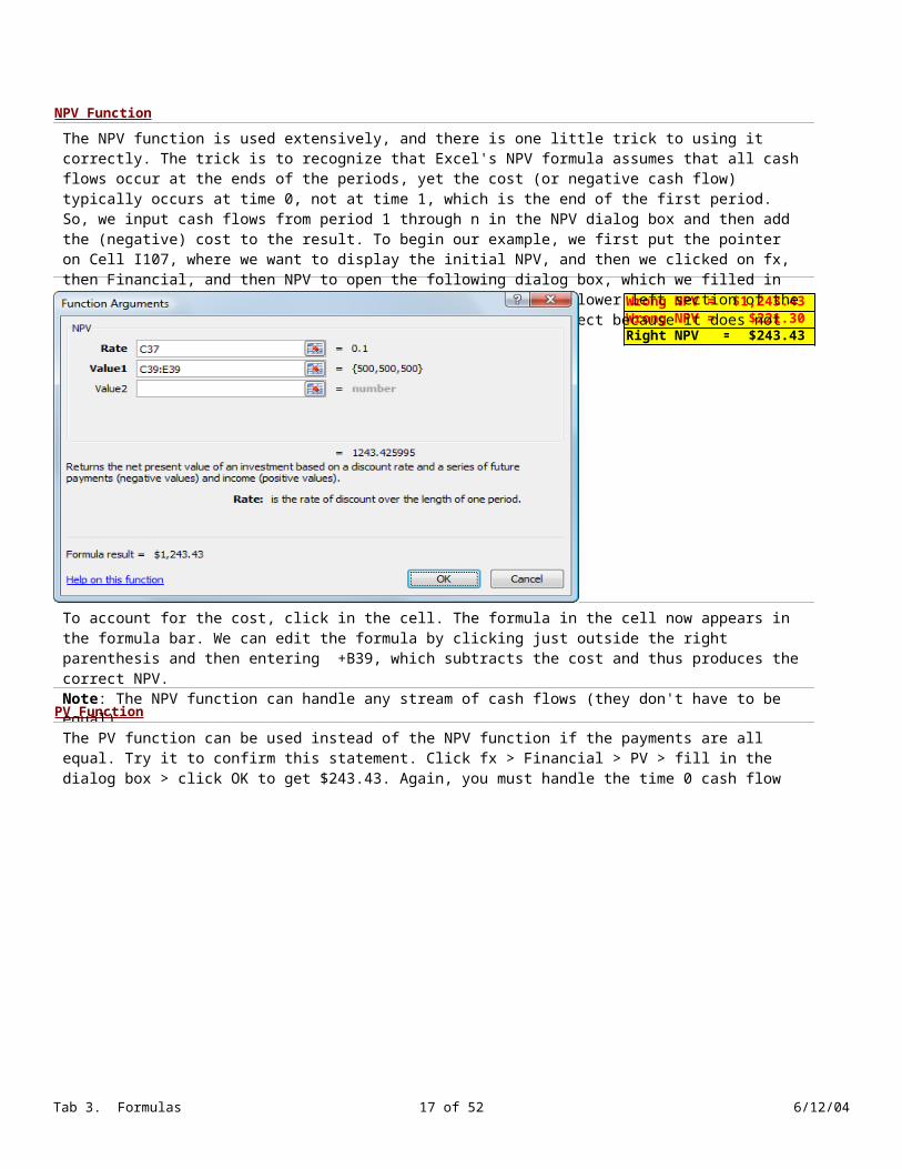
NPV Function

Wrong NPV = $1,243.43 Wrong NPV = $221.30 Right NPV = $243.43

PV Function

The NPV function is used extensively, and there is one little trick to using it correctly. The trick is to recognize that Excel's NPV formula assumes that all cash flows occur at the ends of the periods, yet the cost (or negative cash flow) typically occurs at time 0, not at time 1, which is the end of the first period. So, we input cash flows from period 1 through n in the NPV dialog box and then add the (negative) cost to the result. To begin our example, we first put the pointer on Cell I107, where we want to display the initial NPV, and then we clicked on fx, then Financial, and then NPV to open the following dialog box, which we filled in with data provided on Rows 37 through 39. As shown in the lower left section of the dialog box, the initial NPV is $1,243.43, but it is incorrect because it does not reflect the cost of the investment.

To account for the cost, click in the cell. The formula in the cell now appears in the formula bar. We can edit the formula by clicking just outside the right parenthesis and then entering +B39, which subtracts the cost and thus produces the correct NPV. Note: The NPV function can handle any stream of cash flows (they don't have to be equal).

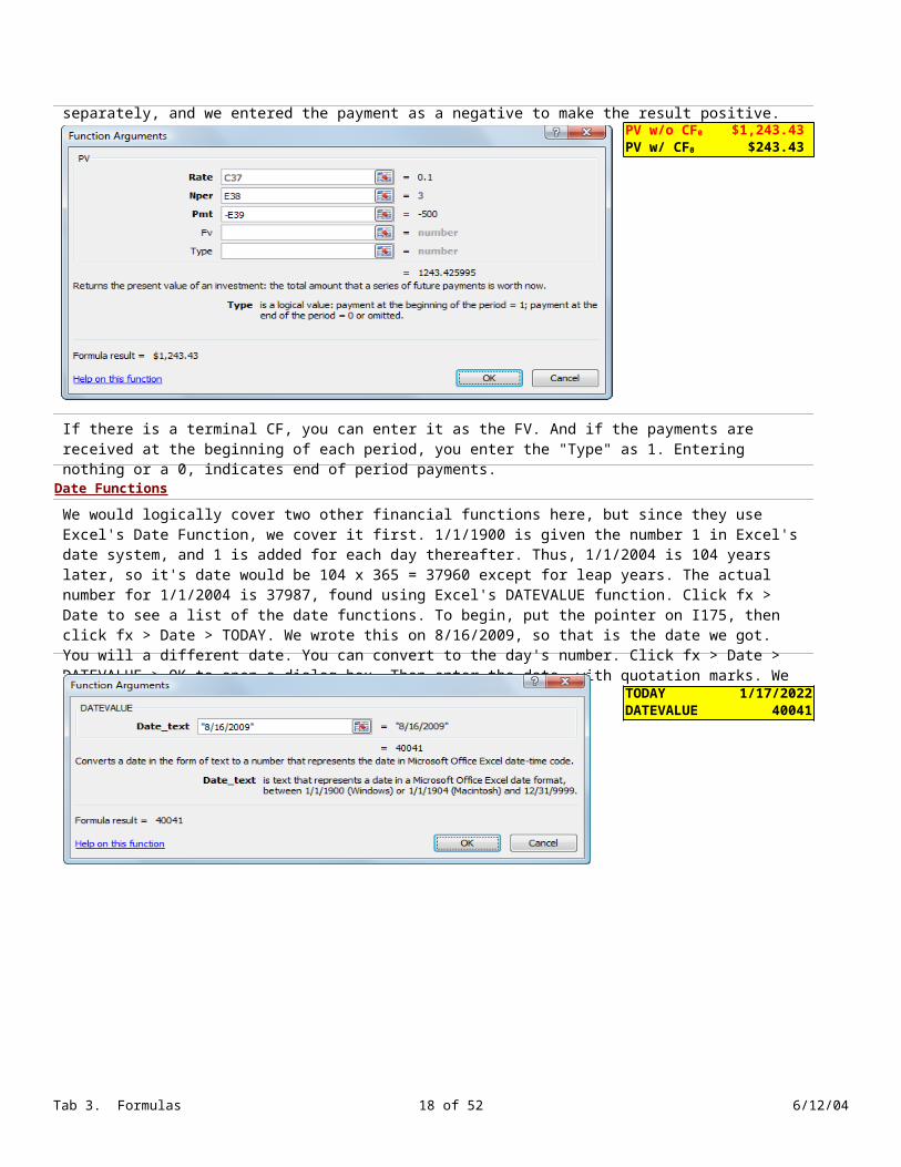
The PV function can be used instead of the NPV function if the payments are all equal. Try it to confirm this statement. Click fx > Financial > PV > fill in the dialog box > click OK to get $243.43. Again, you must handle the time 0 cash flow separately, and we entered the payment as a negative to make the result positive.

This wrong NPV uses the formula correctly but forgets to add in the initial CF.

This wrong NPV includes the initial CF in the NPV calculation. Remember, you must start with the Yr1 CF and add the initial CF after the formula.

I101

This wrong NPV uses the formula correctly but forgets to add in the initial CF.

I102

This wrong NPV includes the initial CF in the NPV calculation. Remember, you must start with the Yr1 CF and add the initial CF after the formula.


$1,243.43 $243.43

Date Functions

TODAY 4/9/2023DATEVALUE 40041

PV w/o CF0

PV w/ CF0

The PV function can be used instead of the NPV function if the payments are all equal. Try it to confirm this statement. Click fx > Financial > PV > fill in the dialog box > click OK to get $243.43. Again, you must handle the time 0 cash flow separately, and we entered the payment as a negative to make the result positive.

If there is a terminal CF, you can enter it as the FV. And if the payments are received at the beginning of each period, you enter the "Type" as 1. Entering nothing or a 0, indicates end of period payments.

We would logically cover two other financial functions here, but since they use Excel's Date Function, we cover it first. 1/1/1900 is given the number 1 in Excel's date system, and 1 is added for each day thereafter. Thus, 1/1/2004 is 104 years later, so it's date would be 104 x 365 = 37960 except for leap years. The actual number for 1/1/2004 is 37987, found using Excel's DATEVALUE function. Click fx > Date to see a list of the date functions. To begin, put the pointer on I175, then click fx > Date > TODAY. We wrote this on 8/16/2009, so that is the date we got. You will a different date. You can convert to the day's number. Click fx > Date > DATEVALUE > OK to open a dialog box. Then enter the date, with quotation marks. We entered our date as follows:

The date function is used for many purposes. For example, you can subtract one datevalue from another to determine the days of interest on a loan, and Excel uses the procedure to find the price and yield on bonds, as we discuss below.


Bond Price and Yield Functions

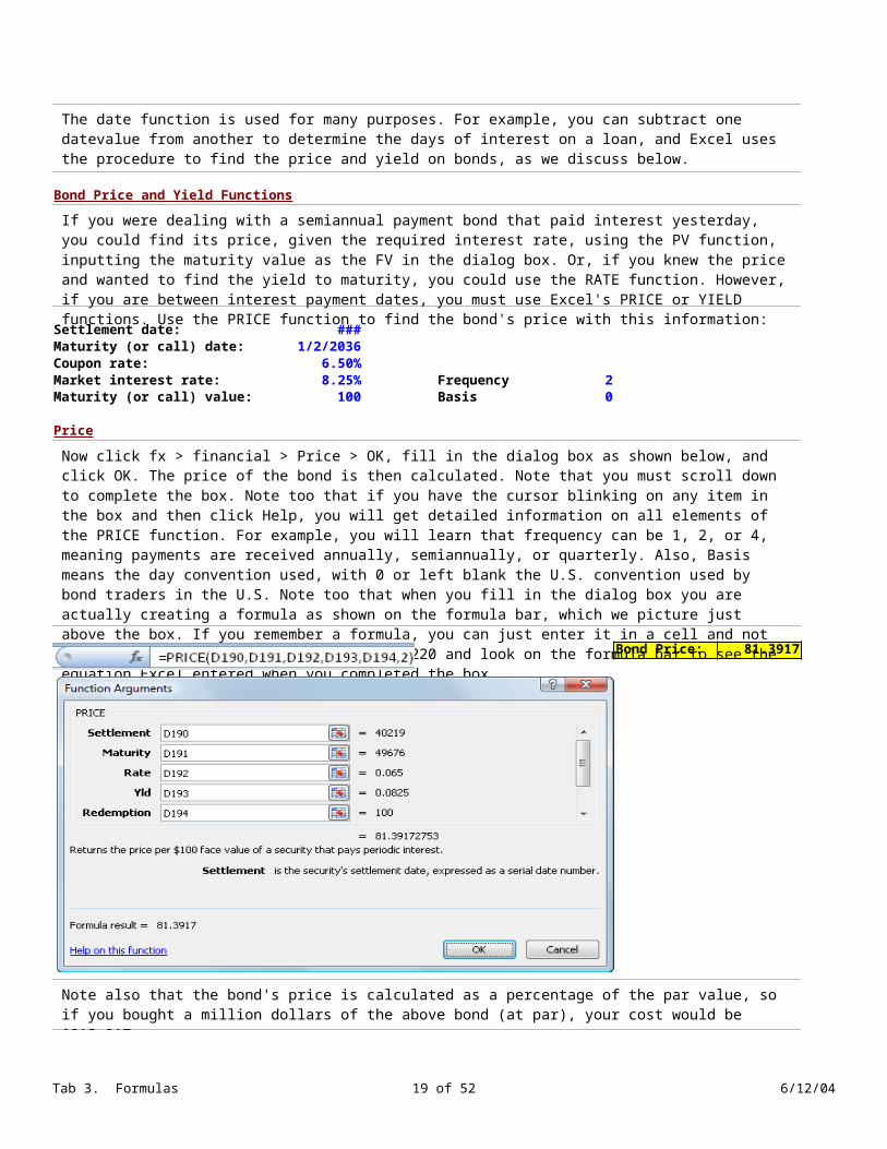
Settlement date: 2/10/2010Maturity (or call) date: 1/2/2036Coupon rate: 6.50%Market interest rate: 8.25% Frequency 2Maturity (or call) value: 100 Basis 0

Price

Bond Price: 81.3917

The date function is used for many purposes. For example, you can subtract one datevalue from another to determine the days of interest on a loan, and Excel uses the procedure to find the price and yield on bonds, as we discuss below.

If you were dealing with a semiannual payment bond that paid interest yesterday, you could find its price, given the required interest rate, using the PV function, inputting the maturity value as the FV in the dialog box. Or, if you knew the price and wanted to find the yield to maturity, you could use the RATE function. However, if you are between interest payment dates, you must use Excel's PRICE or YIELD functions. Use the PRICE function to find the bond's price with this information:

Now click fx > financial > Price > OK, fill in the dialog box as shown below, and click OK. The price of the bond is then calculated. Note that you must scroll down to complete the box. Note too that if you have the cursor blinking on any item in the box and then click Help, you will get detailed information on all elements of the PRICE function. For example, you will learn that frequency can be 1, 2, or 4, meaning payments are received annually, semiannually, or quarterly. Also, Basis means the day convention used, with 0 or left blank the U.S. convention used by bond traders in the U.S. Note too that when you fill in the dialog box you are actually creating a formula as shown on the formula bar, which we picture just above the box. If you remember a formula, you can just enter it in a cell and not use the dialog box. Put the pointer on I220 and look on the formula bar to see the equation Excel entered when you completed the box.

Note also that the bond's price is calculated as a percentage of the par value, so if you bought a million dollars of the above bond (at par), your cost would be $813,917.


Yield

Now assume that you have the following information and want to determine the bond's yield to maturity. Click Financial > Yield > OK and then fill in the box as shown below. Note that if the bond were callable, you could use the call price for "Redemption" and the call date for the maturity date and then calculate the yield to call.


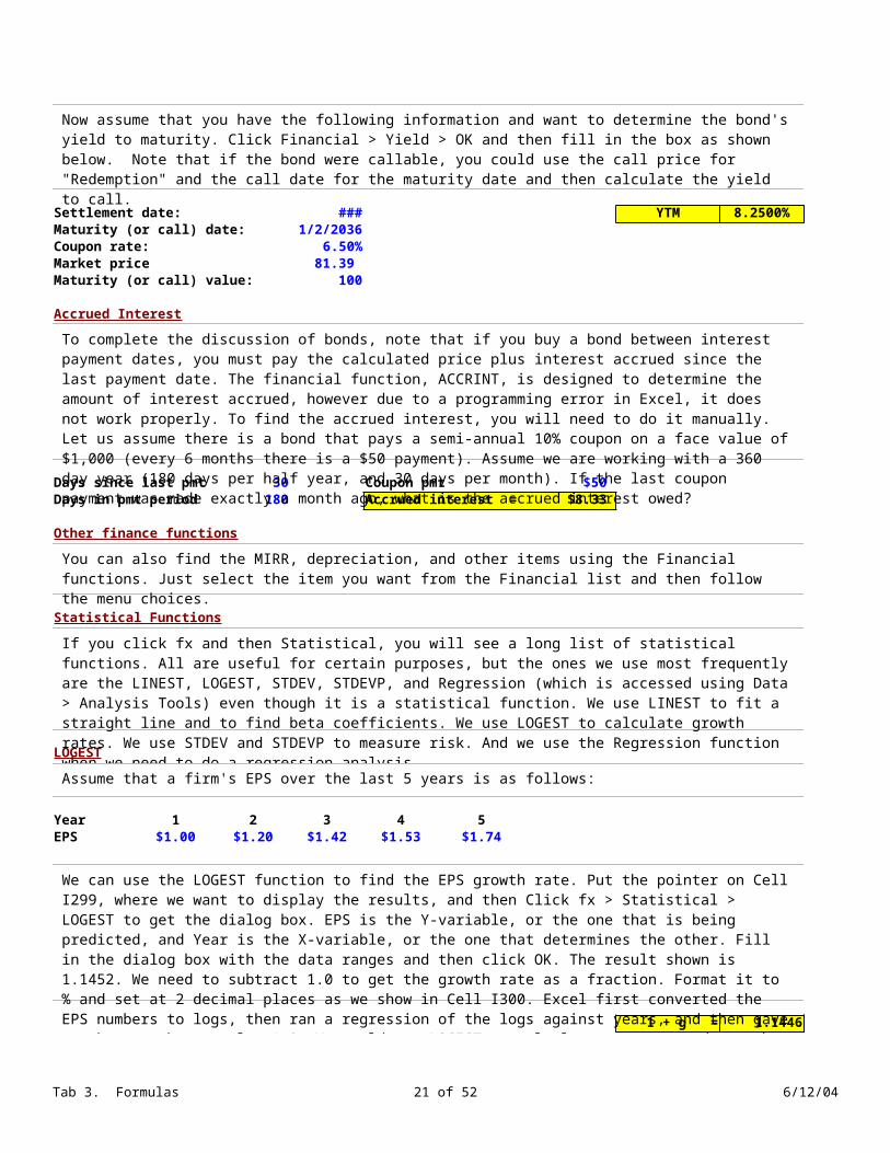
Settlement date: 2/10/2010 YTM 8.2500%Maturity (or call) date: 1/2/2036Coupon rate: 6.50%Market price 81.39 Maturity (or call) value: 100

Accrued Interest

Days since last pmt 30 Coupon pmt $50 Days in pmt period 180 Accrued interest = $8.33

Other finance functions

Statistical Functions

LOGEST

Year 1 2 3 4 5EPS $1.00 $1.20 $1.42 $1.53 $1.74

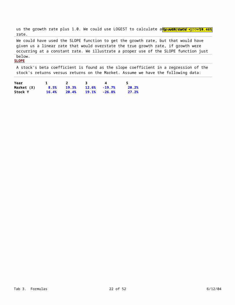
1 + g = 1.1446Growth rate = 14.46%

Now assume that you have the following information and want to determine the bond's yield to maturity. Click Financial > Yield > OK and then fill in the box as shown below. Note that if the bond were callable, you could use the call price for "Redemption" and the call date for the maturity date and then calculate the yield to call.

To complete the discussion of bonds, note that if you buy a bond between interest payment dates, you must pay the calculated price plus interest accrued since the last payment date. The financial function, ACCRINT, is designed to determine the amount of interest accrued, however due to a programming error in Excel, it does not work properly. To find the accrued interest, you will need to do it manually. Let us assume there is a bond that pays a semi-annual 10% coupon on a face value of $1,000 (every 6 months there is a $50 payment). Assume we are working with a 360 day year (180 days per half year, and 30 days per month). If the last coupon payment was made exactly a month ago, what is the accrued interest owed?

You can also find the MIRR, depreciation, and other items using the Financial functions. Just select the item you want from the Financial list and then follow the menu choices.

If you click fx and then Statistical, you will see a long list of statistical functions. All are useful for certain purposes, but the ones we use most frequently are the LINEST, LOGEST, STDEV, STDEVP, and Regression (which is accessed using Data > Analysis Tools) even though it is a statistical function. We use LINEST to fit a straight line and to find beta coefficients. We use LOGEST to calculate growth rates. We use STDEV and STDEVP to measure risk. And we use the Regression function when we need to do a regression analysis.

Assume that a firm's EPS over the last 5 years is as follows:

We can use the LOGEST function to find the EPS growth rate. Put the pointer on Cell I299, where we want to display the results, and then Click fx > Statistical > LOGEST to get the dialog box. EPS is the Y-variable, or the one that is being predicted, and Year is the X-variable, or the one that determines the other. Fill in the dialog box with the data ranges and then click OK. The result shown is 1.1452. We need to subtract 1.0 to get the growth rate as a fraction. Format it to % and set at 2 decimal places as we show in Cell I300. Excel first converted the EPS numbers to logs, then ran a regression of the logs against years, and then gave us the growth rate plus 1.0. We could use LOGEST to calculate any compound growth rate.


SLOPE

Year 1 2 3 4 5Market (X) 8.5% 19.3% 12.6% -19.7% 20.2%Stock Y 16.4% 20.4% 19.1% -26.8% 27.2%

We could have used the SLOPE function to get the growth rate, but that would have given us a linear rate that would overstate the true growth rate, if growth were occurring at a constant rate. We illustrate a proper use of the SLOPE function just below.

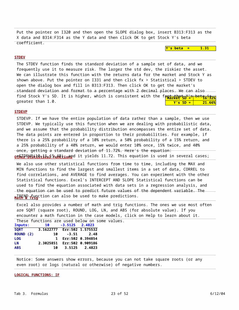
A stock's beta coefficient is found as the slope coefficient in a regression of the stock's returns versus returns on the Market. Assume we have the following data:

Put the pointer on I320 and then open the SLOPE dialog box, insert B313:F313 as the X data and B314:F314 as the Y data and then click OK to get Stock Y's beta coefficient.


Y's beta = 1.31

STDEV

Market SD = 16.32%Y's SD = 21.66%

STDEVP

Other Statistical Functions

Math & Trig

Inputs: 10 -3.5125 2.4823SQRT 3.16227766 Err:502 1.5755317ROUND (2) 10 -3.51 2.48LOG 1 Err:502 0.3948543LN 2.30258509 Err:502 0.9091855ABS 10 3.5125 2.4823

LOGICAL FUNCTIONS: IF

Put the pointer on I320 and then open the SLOPE dialog box, insert B313:F313 as the X data and B314:F314 as the Y data and then click OK to get Stock Y's beta coefficient.

The STDEV function finds the standard deviation of a sample set of data, and we frequently use it to measure risk. The larger the std dev, the riskier the asset. We can illustrate this function with the returns data for the market and Stock Y as shown above. Put the pointer on I331 and then click fx > Statistical > STDEV to open the dialog box and fill in B313:F313. Then click OK to get the market's standard deviation and format to a percentage with 2 decimal places. We can also find Stock Y's SD. It is higher, which is consistent with the fact that Y's beta is greater than 1.0.

STDEVP. If we have the entire population of data rather than a sample, then we use STDEVP. We typically use this function when we are dealing with probabilistic data, and we assume that the probability distribution encompasses the entire set of data. The data points are entered in proportion to their probabilities. For example, if there is a 25% probability of a 10% return, a 50% probability of a 15% return, and a 25% probability of a 40% return, we would enter 10% once, 15% twice, and 40% once, getting a standard deviation of 11.72%. Here's the equation: =STDEVP(10,15,15,40), and it yields 11.72. This equation is used in several cases; see Case 2 model for an illustration.

We also use other statistical functions from time to time, including the MAX and MIN functions to find the largest and smallest items in a set of data, CORREL to find correlations, and AVERAGE to find averages. You can experiment with the other Statistical functions. Excel's INTERCEPT AND SLOPE Statistical functions can be used to find the equation associated with data sets in a regression analysis, and the equation can be used to predict future values of the dependent variable. The TREND function can also be used to make predictions.

Excel also provides a number of math and trig functions. The ones we use most often are SQRT (square root), ROUND, LOG, LN, and ABS (for absolute value). If you encounter a math function in the case models, click on Help to learn about it. These functions are used below on some values.

Notice: Some answers show errors, because you can not take square roots (or any even root) or logs (natural or otherwise) of negative numbers.

Click fx > Logical to see the available logical functions. We use IF frequently in the cases. Here is an example where we use IF, along with the ABS math function and the MAX statistical function, to find the payback of a project:


Year 0 1 2 3 4 5Cash flow -$1,000 $300 $300 $300 $300 $300Cumulative CF -$1,000 -$700 -$400 -$100 $200 $500Payback 3.33 - - - - 3.33 -

Click fx > Logical to see the available logical functions. We use IF frequently in the cases. Here is an example where we use IF, along with the ABS math function and the MAX statistical function, to find the payback of a project:

The years and cash flows are the inputs. We first calculate the cumulative CFs. We can see by inspection that the payback is 3 years plus a fraction, with the fraction being (unrecovered after 3) / (CF in 4) = 0.333. It's easy to find the payback of a single project, but if we are examining many projects, and especially if we would like to find their paybacks if conditions change as they would in a sensitivity analysis, then it would be good to automate the process. This we do on Rows 378 and 379. On Row 286 we use the IF dialog box to insert this formula in G379:


=IF(G378<0,"-",IF(F378<0,G376-1+ABS(F378)/G377,"-"))

REGRESSION (Simple)

Year 1 2 3 4 5Market (X) 8.5% 15.3% 12.6% -5.7% 20.2%Stock Y 10.4% 18.4% 15.1% -6.8% 24.2%

The years and cash flows are the inputs. We first calculate the cumulative CFs. We can see by inspection that the payback is 3 years plus a fraction, with the fraction being (unrecovered after 3) / (CF in 4) = 0.333. It's easy to find the payback of a single project, but if we are examining many projects, and especially if we would like to find their paybacks if conditions change as they would in a sensitivity analysis, then it would be good to automate the process. This we do on Rows 378 and 379. On Row 286 we use the IF dialog box to insert this formula in G379:

The formula first checks to see if the cumulative CF at the end of a year is negative. If it is, we have not yet reached the payback so we insert a dash. If the cumulative CF is positive, we check to see if the prior year's cumulative CF was negative, and if it was, we are at the payback year. We then get the prior year's number and add to it a fraction equal to the ABS value of the prior year's deficit divided by the current year's CF. This is the actual payback, and it is entered into the cell on Row 379. If the prior year's cumulative CF was positive,then we have passed the payback year, so we insert a dash. Finally, we use the MAX function to insert the payback into cell B379.

If you do much with Excel, you will find many uses for the IF statement and other logical functions. There are often a lot of ways to do something, and it often takes us a while to come up with the best procedure. That was true for the payback calculation shown above.

Although regression is a statistical procedure, Excel provides it under the Data Analysis on the Data tab. Click the Data Analysis button and then choose Regression. If the Analysis ToolPak add-in is not installed on your computer, you must install it as an "Add-in." Click help and then enter "analysis toolpak" as the search term and then follow the instructions. We use the same returns data that we used to calculate beta in our regression illustration.

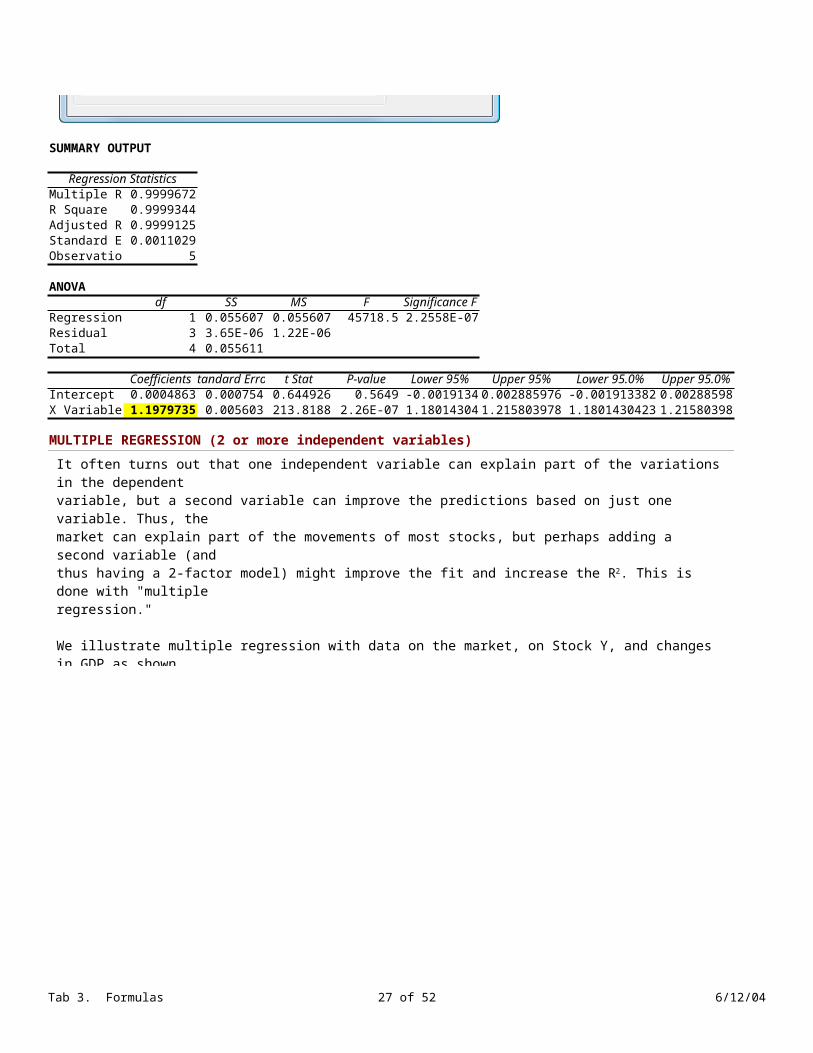
Click Data Analysis and then Regression to open the dialog box shown below, filled in. Now fill in the X and Y ranges, and then enter A438 as the Output Range. Make sure nothing is in the output range, or it will be overwritten. When you click OK, the regression results will appear beginning on Row 438. The R and R2 as highlighted in the output are both 0.9999, which indicates almost perfect correlation. The beta coefficient is 1.197…, which is the same as we calculated earlier. Other statistics are also shown in the output, and still more could have been calculated had we chosen to do so.



SUMMARY OUTPUT

Regression StatisticsMultiple R 0.99996719R Square 0.99993439Adjusted R S0.99991251Standard Err 0.00110286Observations 5

ANOVAdf SS MS F Significance F

Regression 1 0.0556071 0.0556071 45718.497 2.25579E-07Residual 3 3.649E-06 1.216E-06Total 4 0.0556108

CoefficientsStandard Error t Stat P-value Lower 95% Upper 95% Lower 95.0% Upper 95.0%Intercept 0.0004863 0.000754 0.6449257 0.5648997 -0.00191338 0.002885976 -0.0019133822 0.00288598X Variable 1 1.19797351 0.0056027 213.81884 2.256E-07 1.180143042 1.215803978 1.18014304235 1.21580398

MULTIPLE REGRESSION (2 or more independent variables)

It often turns out that one independent variable can explain part of the variations in the dependentvariable, but a second variable can improve the predictions based on just one variable. Thus, themarket can explain part of the movements of most stocks, but perhaps adding a second variable (andthus having a 2-factor model) might improve the fit and increase the R2. This is done with "multipleregression."

We illustrate multiple regression with data on the market, on Stock Y, and changes in GDP as shownbelow. We regress returns on Stock Y on market returns and GDP changes. If we left out GDP, wewould be working with the CAPM, which is a 1-factor model. Note that we set up Stock Y to the left.Excel's multiple regression program required that the dependent variable be the data to the left, withthe data for the independent variables given to the right.

Click Tools > Data analysis > Regression > OK to open the Regression dialog box. Then enter the range with the Y data, B495:B499. Then enter the range for the independent variables, C495:D499.Then specify where you want the regression output to be displayed, and then click OK. The filled indialog box is shown below, as is the regression output.

Tab 4. Data Tables Graphs 23 of 42 6/12/04

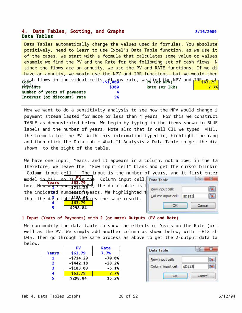
4. Data Tables, Sorting, and Graphs 8/16/2009Data Tables

Cost -$1,000 PV (or NPV) $63.79 Payments $300 Rate (or IRR) 7.7%Number of years of payments 4Interest (or discount) rate 5%

PVYears $63.79

1 -$714.292 -$442.183 -$183.034 $63.795 $298.84

1 Input (Years of Payments) with 2 (or more) Outputs (PV and Rate)

PV RateYears $63.79 7.7%

1 -$714.29 -70.0%2 -$442.18 -28.2%3 -$183.03 -5.1%4 $63.79 7.7%5 $298.84 15.2%

Data Tables automatically change the values used in formulas. You absolutely, positively, need to learn to use Excel's Data Table function, as we use it in all of the cases. We start with a formula that calculates some value or values; in our example we find the PV and the Rate for the following set of cash flows. Note that since the flows are an annuity, we use the PV and RATE functions. If we did not have an annuity, we would use the NPV and IRR functions, but we would then have the cash flows in individual cells. At any rate, we find the NPV and IRR as shown below.

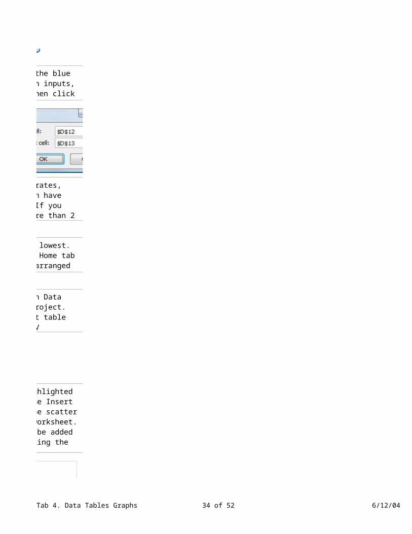
Now we want to do a sensitivity analysis to see how the NPV would change if the payment stream lasted for more or less than 4 years. For this we construct a DATA TABLE as demonstrated below. We begin by typing in the items shown in BLUE--the labels and the number of years. Note also that in cell C31 we typed =H11, which is the formula for the PV. With this information typed in, highlight the range B31:C36 and then click the Data tab > What-If Analysis > Data Table to get the dialog box shown to the right of the table.

We have one input, Years, and it appears in a column, not a row, in the table. Therefore, we leave the "Row input cell" blank and get the cursor blinking in the "Column input cell." The input is the number of years, and it first enters the model in D13, so D13 is the Column input cell, as we show in the completed dialog box. Now when you click OK, the data table is filled in with the PVs for each of the indicated number of years. We highlighted the PV for the base case to show that the data table produces the same result.

We can modify the data table to show the effects of Years on the Rate (or IRR) as well as the PV. We simply add another column as shown below, with =H12 shown in D45. Then go through the same process as above to get the 2-output data table shown below.


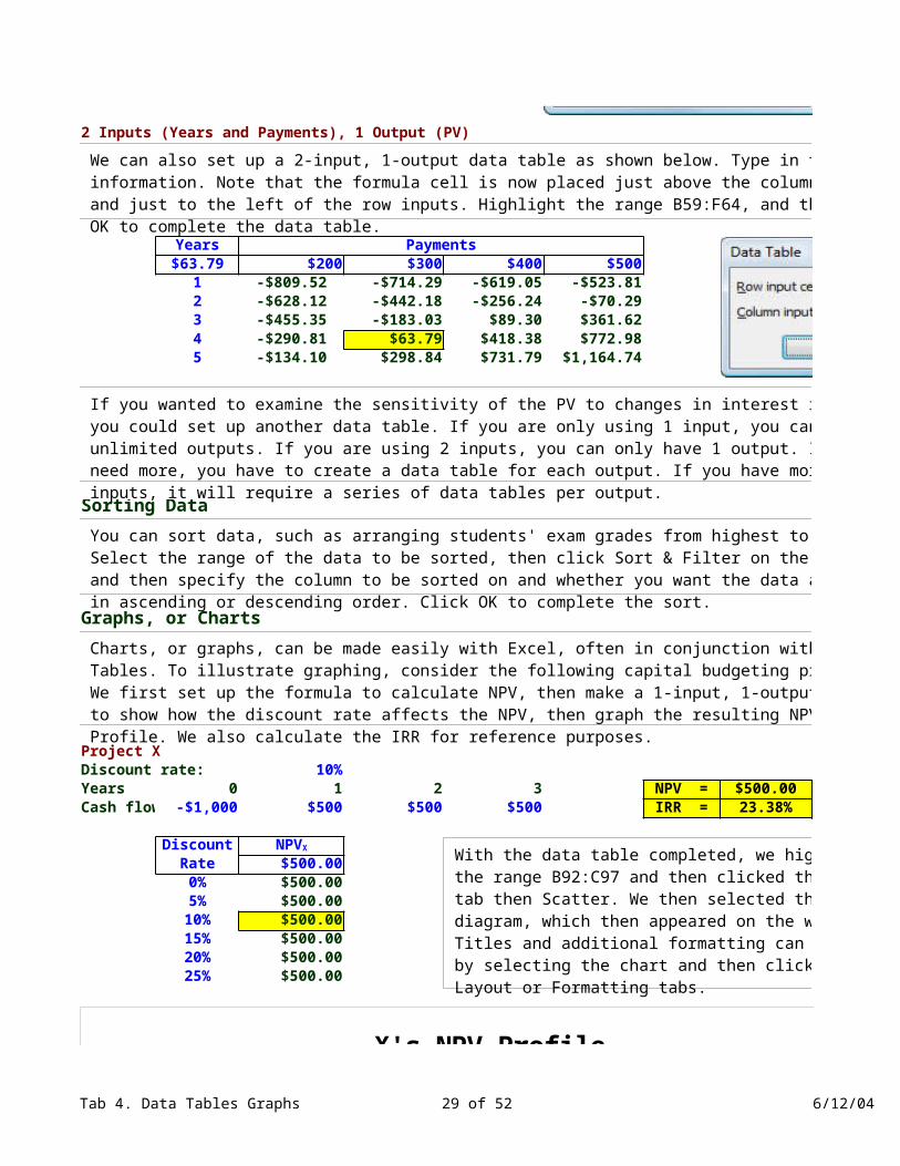
2 Inputs (Years and Payments), 1 Output (PV)

Years Payments$63.79 $200 $300 $400 $500

1 -$809.52 -$714.29 -$619.05 -$523.812 -$628.12 -$442.18 -$256.24 -$70.293 -$455.35 -$183.03 $89.30 $361.624 -$290.81 $63.79 $418.38 $772.985 -$134.10 $298.84 $731.79 $1,164.74

Sorting Data

Graphs, or Charts

Project XDiscount rate: 10%Years 0 1 2 3 NPV = $500.00Cash flow -$1,000 $500 $500 $500 IRR = 23.38%

DiscountRate $500.000% $500.005% $500.00

10% $500.0015% $500.0020% $500.0025% $500.00

NPVX

We can also set up a 2-input, 1-output data table as shown below. Type in the blue information. Note that the formula cell is now placed just above the column inputs, and just to the left of the row inputs. Highlight the range B59:F64, and then click OK to complete the data table.

If you wanted to examine the sensitivity of the PV to changes in interest rates, you could set up another data table. If you are only using 1 input, you can have unlimited outputs. If you are using 2 inputs, you can only have 1 output. If you need more, you have to create a data table for each output. If you have more than 2 inputs, it will require a series of data tables per output.

You can sort data, such as arranging students' exam grades from highest to lowest. Select the range of the data to be sorted, then click Sort & Filter on the Home tab and then specify the column to be sorted on and whether you want the data arranged in ascending or descending order. Click OK to complete the sort.

Charts, or graphs, can be made easily with Excel, often in conjunction with Data Tables. To illustrate graphing, consider the following capital budgeting project. We first set up the formula to calculate NPV, then make a 1-input, 1-output table to show how the discount rate affects the NPV, then graph the resulting NPV Profile. We also calculate the IRR for reference purposes.

0% 5% 10% 15% 20% 25% 30%$0.00

$100.00$200.00$300.00$400.00$500.00$600.00

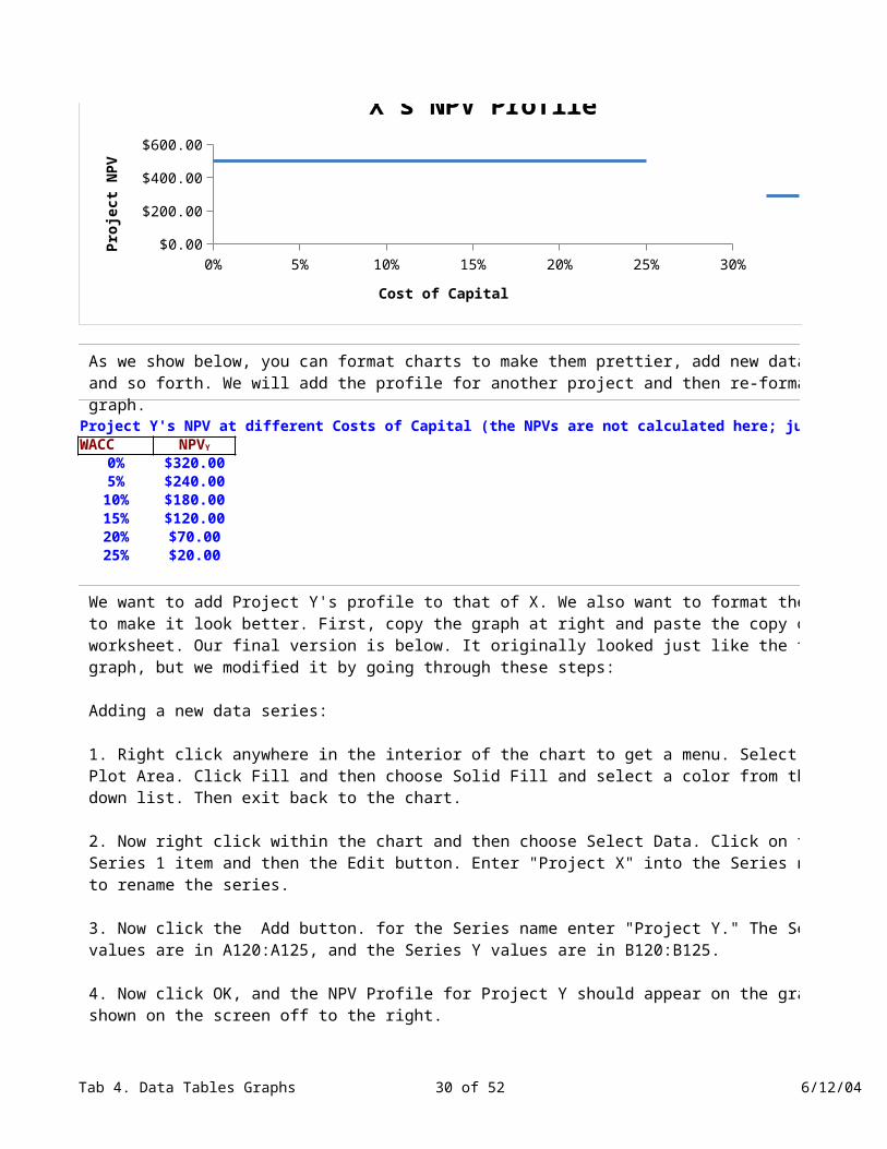
X's NPV Profile

Column C

Cost of Capital

Proj

ect N

PV

With the data table completed, we highlighted the range B92:C97 and then clicked the Insert tab then Scatter. We then selected the scatter diagram, which then appeared on the worksheet. Titles and additional formatting can be added by selecting the chart and then clicking the Layout or Formatting tabs.


Project Y's NPV at different Costs of Capital (the NPVs are not calculated here; just take as given):WACC

0% $320.005% $240.00

10% $180.0015% $120.0020% $70.0025% $20.00

NPVY

0% 5% 10% 15% 20% 25% 30%$0.00

$100.00$200.00$300.00$400.00$500.00$600.00

X's NPV Profile

Column C

Cost of Capital

Proj

ect N

PV

As we show below, you can format charts to make them prettier, add new data series, and so forth. We will add the profile for another project and then re-format the graph.

We want to add Project Y's profile to that of X. We also want to format the chart to make it look better. First, copy the graph at right and paste the copy on the worksheet. Our final version is below. It originally looked just like the top graph, but we modified it by going through these steps:

Adding a new data series:

1. Right click anywhere in the interior of the chart to get a menu. Select Format Plot Area. Click Fill and then choose Solid Fill and select a color from the drop down list. Then exit back to the chart.

2. Now right click within the chart and then choose Select Data. Click on the Series 1 item and then the Edit button. Enter "Project X" into the Series name box to rename the series.

3. Now click the Add button. for the Series name enter "Project Y." The Series X values are in A120:A125, and the Series Y values are in B120:B125.

4. Now click OK, and the NPV Profile for Project Y should appear on the graph as shown on the screen off to the right.

Formatting the chart:

5. Now place the pointer on the Y axis so that the words "Vertical (Value) Axis" appear, and right click. Then select Format Axis. Now you can make the axis information bold face, change the font size, and so forth.

6. Repeat step 5 for the X axis to format the horizontal axis.

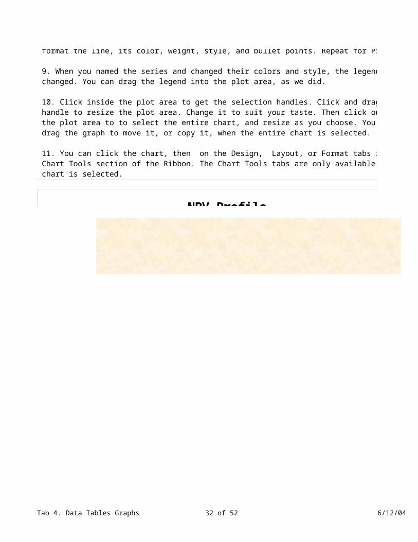
7. Now put the pointer on the profile line for Project X and right click. Then format the line, its color, weight, style, and bullet points. Repeat for Project Y.

9. When you named the series and changed their colors and style, the legends changed. You can drag the legend into the plot area, as we did.

10. Click inside the plot area to get the selection handles. Click and drag a handle to resize the plot area. Change it to suit your taste. Then click outside the plot area to to select the entire chart, and resize as you choose. You can also drag the graph to move it, or copy it, when the entire chart is selected.

11. You can click the chart, then on the Design, Layout, or Format tabs in the Chart Tools section of the Ribbon. The Chart Tools tabs are only available while a chart is selected.

12. On this graph there is no real need to adjust the range of the X and Y values as shown, but to demonstrate the procedure we contract the X range from 0 to 30 to 0 to 25. Right click the X axis, and then choose Format Axis. At the top of the Axis Options you can then change the maximum from 0.3 to 0.25. The horizontal axis then changes. Our final graph is shown below.

Formatting graphs is fairly simple, although you do have to go through a number of steps. Note, though, that you really don't have to do any formatting at all if all you want to do is see a relation as a picture, because the original graph is OK.

0% 5% 10% 15% 20% 25% 30%$0.00

$100.00

$200.00

$300.00

$400.00

$500.00

$600.00

X's NPV Profile

Project XProject Y

Cost of Capital

Proj

ect N

PV

































0% 5% 10% 15% 20% 25%$0.00

$100.00$200.00$300.00$400.00$500.00$600.00

NPV Profile

Project XProject Y

Cost of Capital

Proj

ect N

PV

Tab 5. Goal Seek 28 of 42 6/12/03

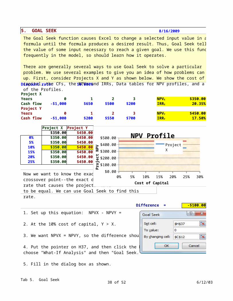
5. GOAL SEEK 8/16/2009

Discount rate: 10.000%

Project XYears 0 1 2 3 $350.00Cash flows -$1,000 $650 $500 $200 20.35%Project YYears 0 1 2 3 $450.00Cash flows -$1,000 $200 $550 $700 17.50%

Project X Project Y$350.00 $450.00

0% $350.00 $450.005% $350.00 $450.00

10% $350.00 $450.0015% $350.00 $450.0020% $350.00 $450.0025% $350.00 $450.00

Difference = -$100.00

NPVX

IRRX

NPVY

IRRY

The Goal Seek function causes Excel to change a selected input value in a formula until the formula produces a desired result. Thus, Goal Seek tells you the value of some input necessary to reach a given goal. We use this function frequently in the model, so should learn how it operates.

There are generally several ways to use Goal Seek to solve a particular problem. We use several examples to give you an idea of how problems can be set up. First, consider Projects X and Y as shown below. We show the cost of capital, the CFs, the NPVs and IRRs, Data tables for NPV profiles, and a graph of the Profiles.

Now we want to know the exact crossover point--the exact discount rate that causes the projects' NPVs to be equal. We can use Goal Seek to find this rate.

1. Set up this equation: NPVX - NPVY =

2. At the 10% cost of capital, Y > X.

3. We want NPVX = NPVY, so the difference should be 0.

4. Put the pointer on H37, and then click the Data tab andchoose "What-If Analysis" and then "Goal Seek."

5. Fill in the dialog box as shown.

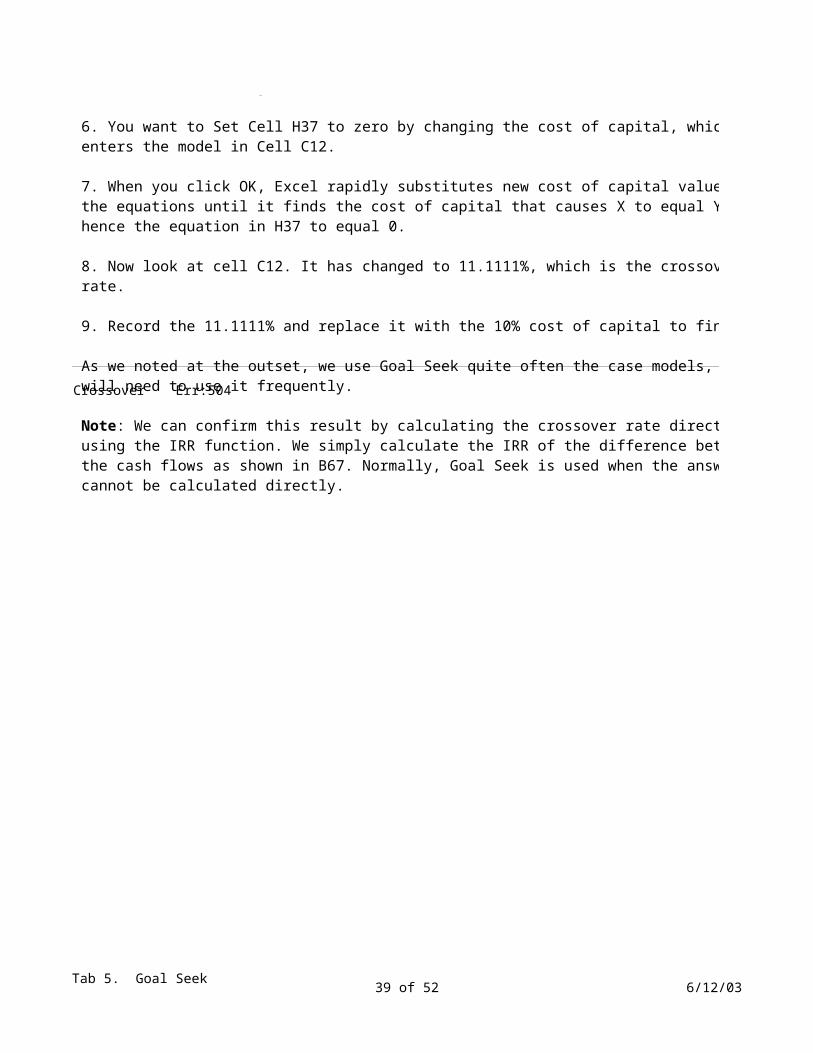
6. You want to Set Cell H37 to zero by changing the cost of capital, which enters the model in Cell C12.

7. When you click OK, Excel rapidly substitutes new cost of capital values into the equations until it finds the cost of capital that causes X to equal Y, hence the equation in H37 to equal 0.

8. Now look at cell C12. It has changed to 11.1111%, which is the crossover rate. 9. Record the 11.1111% and replace it with the 10% cost of capital to finish.

As we noted at the outset, we use Goal Seek quite often the case models, so you will need to use it frequently.

Note: We can confirm this result by calculating the crossover rate directly, using the IRR function. We simply calculate the IRR of the difference between the cash flows as shown in B67. Normally, Goal Seek is used when the answer cannot be calculated directly.

0% 5% 10% 15% 20% 25% 30%$0.00

$100.00

$200.00

$300.00

$400.00

$500.00NPV Profile

Project X

Project Y

Cost of Capital

Proj

ect N

PV

Tab 5. Goal Seek 29 of 42 6/12/03

Crossover Err:504











Tab 5. Goal Seek 30 of 42 6/12/03

The Goal Seek function causes Excel to change a selected input value in a formula until the formula produces a desired result. Thus, Goal Seek tells you the value of some input necessary to reach a given goal. We use this function frequently in the model, so should learn how it operates.

There are generally several ways to use Goal Seek to solve a particular problem. We use several examples to give you an idea of how problems can be set up. First, consider Projects X and Y as shown below. We show the cost of capital, the CFs, the NPVs and IRRs, Data tables for NPV profiles, and a graph of the Profiles.











Tab 5. Goal Seek 31 of 42 6/12/03











Tab 6. Scenarios 32 of 42 6/12/04

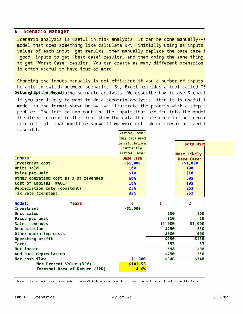
6. Scenario Manager

Setting Up the Model

Active Case:

this data used

in calculations Data Used in the Scenarios:Currently

Active Case: Most Likely:Inputs: Base Case Base Case: Best CaseInvestment cost -$1,000 -$1,000 -$900Units sold 100 100 150Price per unit $10 $10 $12Other operating cost as % of revenues 60% 60% 50%Cost of Capital (WACC) 10% 10% 8%Depreciation rate (constant) 25% 25% 25%Tax rate (constant) 35% 35% 35%

Model: Years 0 1 2 3Investment -$1,000Unit sales 100 100 100Price per unit $10 10 10Sales revenues $1,000 $1,000 $1,000Depreciation $250 250 250Other operating costs $600 600 600Operating profit $150 $150 $150Taxes $53 53 53Net income $98 $98 $98Add back depreciation $250 250 250Net cash flow -$1,000 $348 $348 $348

Net Present Value (NPV) $101.53Internal Rate of Return (IRR) 14.6%

Scenario analysis is useful in risk analysis. It can be done manually--simply set up a model that does something like calculate NPV, initially using as inputs the most likely values of each input, get results, then manually replace the base case inputs with a set of "good" inputs to get "best case" results, and then doing the same thing with "bad" inputs to get "Worst Case" results. You can create as many different scenarios as you want, and it is often useful to have four or more.

Changing the inputs manually is not efficient if you a number of inputs and/or you want to be able to switch between scenarios. So, Excel provides a tool called "Scenario Manager" that facilitates doing scenario analysis. We describe how to use Scenario Manager in this tutorial.

If you are likely to want to do a scenario analysis, then it is useful to set up your basic model in the format shown below. We illustrate the process with a simple capital budgeting problem. The left column contains the inputs that are fed into the model, and the data in the three columns to the right show the data that are used in the scenarios. The left column is all that would be shown if we were not making scenarios, and it shows the base case data.

Now we want to see what would happen under the good and bad conditions. You could over-type the base case data in Column F to change the model, but if you needed to go back to the base case, you would have to re-enter those numbers. It would be easier to use Scenario Manager, proceeding as follows:




Using Scenario Manager when scenarios have already been created (as they have here):

Creating scenarios:

Summary

1. Click Data tab > Scenario Manager to get the dialog box to the right, and highlight the case you want to see. Then click "Show," and the data in Column D as well as all data in the tables below will instantly change. Click close to exit Scenario Manager and analyze results under the selected scenario.

2. When you are ready to change scenarios, click Data tab > Scenario Manager , highlight the scenario you want, click "Show," and then "Close." If you manually change inputs in Column D, you can quickly return to the Base Case as indicated above.

1. Set up the model with Active Data cells and Scenario Data as we have done. Start with the base case data in the active data column. Include the scenario's name.

2. In the calculation section of the model, enter all values as cell references to the Active Data. Then, when data in the Active Data cells change, so will the calculations.

3. Click Data tab > Scenario Manager to open Scenario Manager. The second dialog box to the right will appear.

4. Click "Add" and the dialog box will appear. Name your scenario, and then select the range of cells in the Active Data column. In our scenario, it was E26:E31. Click OK. The fourth dialog box to the right will appear. It will automatically show the values used for the Base Case scenario. Click OK.

5. Now click the Add button and name the scenario Best Case.

6. Then enter the numbers from the Best Case column to complete the scenario.

7. Repeat the process to create the Bad scenario.

8. Now you can highlight any of the scenario names, click "Show", and the Scenario Manager will instantly put the appropriate inputs into the Active column and thus into the model, hence calculate the NPV for that scenario. Click "Close" to exit Scenario Manager so you can move around the worksheet.

9. You can delete scenarios, edit them, or add new ones at any time. To edit, click Edit on the Scenario Manager box and then change the inputs you want to change.

10. Before saving the workbook, be sure to change the scenario back to the Base Case version to avoid confusion the next time you use the workbook.

Finally, Excel will give you a summary of the scenarios if you want one. Click the "Summary" key at the bottom of the Scenario Manager box, specify the cell where your key output or outputs are located,and click OK. We did that--see the last dialog box to the right. We got a summary on a separate worksheet, and copied the information as shown below. You could edit the summary to do things like add the names of the variables.


Scenario SummaryCurrent Values: Base Case Best Case Worst Case

Changing Cells:$E$26 Base Case Base Case Best Case Worst Case$E$27 -$1,000 -$1,000 -$900 -$1,000$E$28 100 100 150 50$E$29 $10 $10 $12 $10$E$30 60% 60% 50% 70%$E$31 10% 10% 80% 12%

Result Cells:$E$47 $101.53 $101.53 -$149.35 -$438.09$E$48 14.6% 14.6% 63.4% -11.0%

Notes: Current Values column represents values of changing cells attime Scenario Summary Report was created. Changing cells for eachscenario are highlighted in gray.

Created by Timothy R. Mayes, Ph.D. on 8/17/2009





8/16/2009

Data Used in the Scenarios:

Worst Case-$1,000

50$1070%12%25%35%

4

10010

$1,000250600

$15053

$98250

$348

Scenario analysis is useful in risk analysis. It can be done manually--simply set up a model that does something like calculate NPV, initially using as inputs the most likely values of each input, get results, then manually replace the base case inputs with a set of "good" inputs to get "best case" results, and then doing the same thing with "bad" inputs to get "Worst Case" results. You can create as many different scenarios as you want, and it is often useful to have four or more.

Changing the inputs manually is not efficient if you a number of inputs and/or you want to be able to switch between scenarios. So, Excel provides a tool called "Scenario Manager" that facilitates doing scenario analysis. We describe how to use Scenario Manager in this tutorial.

If you are likely to want to do a scenario analysis, then it is useful to set up your basic model in the format shown below. We illustrate the process with a simple capital budgeting problem. The left column contains the inputs that are fed into the model, and the data in the three columns to the right show the data that are used in the scenarios. The left column is all that would be shown if we were not making scenarios, and it shows the base case data.





1. Click Data tab > Scenario Manager to get the dialog box to the right, and highlight the case you want to see. Then click "Show," and the data in Column D as well as all data in the tables below will instantly change. Click close to exit Scenario Manager and analyze results under the selected scenario.

2. When you are ready to change scenarios, click Data tab > Scenario Manager , highlight the scenario you want, click "Show," and then "Close." If you manually change inputs in Column D, you can quickly return to the Base Case as indicated above.

1. Set up the model with Active Data cells and Scenario Data as we have done. Start with the base case data in the active data column. Include the scenario's name.

2. In the calculation section of the model, enter all values as cell references to the Active Data. Then, when data in the Active Data cells change, so will the calculations.

3. Click Data tab > Scenario Manager to open Scenario Manager. The second dialog box to the right will appear.

4. Click "Add" and the dialog box will appear. Name your scenario, and then select the range of cells in the Active Data column. In our scenario, it was E26:E31. Click OK. The fourth dialog box to the right will appear. It will automatically show the values used for the Base Case scenario. Click OK.

5. Now click the Add button and name the scenario Best Case.

6. Then enter the numbers from the Best Case column to complete the scenario.

7. Repeat the process to create the Bad scenario.

8. Now you can highlight any of the scenario names, click "Show", and the Scenario Manager will instantly put the appropriate inputs into the Active column and thus into the model, hence calculate the NPV for that scenario. Click "Close" to exit Scenario Manager so you can move around the worksheet.

9. You can delete scenarios, edit them, or add new ones at any time. To edit, click Edit on the Scenario Manager box and then change the inputs you want to change.

10. Before saving the workbook, be sure to change the scenario back to the Base Case version to avoid confusion the next time you use the workbook.





Base Case-$1,000

100$1060%10%


Best Case-$900150$1250%80%


Worst Case-$1,000

50$1070%12%

Documents

Excel 2007 Tutorial