Excel 2007 BASICS for Elementary Statistics: Looking at the Big

c©Brooks/Cole, Cengage LearningExcel 2007 BASICS

for Elementary Statistics: Looking at the Big Picture

By Nancy Pfenning and Melissa M. Sovak

Preview

The first part of Elementary Statistics: Looking at the Big Picture, on Data Pro-duction, does not call for the use of statistical software. For this reason, our first chapterconsists of basic tips, such as how to enter and manipulate data. Parts 2, 3, and 4 of thisguide parallel Parts II, III, and IV of the textbook, presenting examples and activities onDisplaying and Summarizing, Probability, and Inference. Within Part 2 on Displaying andSummarizing, and Part 4 on Statistical Inference, methods are presented in sequence foreach of the five variable situations: C, Q, C→Q, C→C, Q→Q.

Part 1: Warming Up with Excel

After starting Excel, you’ll see a sheet, named Sheet1. At the bottom of the screen, you’llsee tabs for two other sheets, Sheet2 and Sheet3, as well as a tab to create new sheets. Thesethree worksheets, along with any other worksheets you create are part of the workbook. Theworksheet is where we enter, name, view and edit. The Office button is located in the topleft corner. The Office button contains menu items to open a new or existing workbook,save the current workbook, print a worksheet, access Excel options among other options.When the save option is selected, Excel will save the entire workbook, not as individualworksheets. However, when printing, Excel will only print the currently selected worksheet,not the entire workbook.

To the right of the Office button, is the menu bar. The menu bar contains the mainmenus: Home, Insert, Page Layout, Formulas, Data, Review and View. To access help forExcel, click the question mark on the right side of the menu bar. Clicking on any of themain menu titles opens several menu options beneath the menu bar. The menu bar is alsowhere submenus appear to edit graphics.

We will often use the Insert Function option, available under the Formulas main menu.The Insert Function option will open a dialog box where you can find and select the functionyou would like to use. If the function that you would like to use is not already listed inSelect a function box, you can search for the function in the Search for a function box bysimply typing the name of the function and pressing Go.

Entering and Manipulating Data

Each variable is stored in a column, designated by a letter. For example, A is the firstcolumn, B is the second, etc. The column designations are displayed along the top of theworksheet.

1

c©Brooks/Cole, Cengage Learning

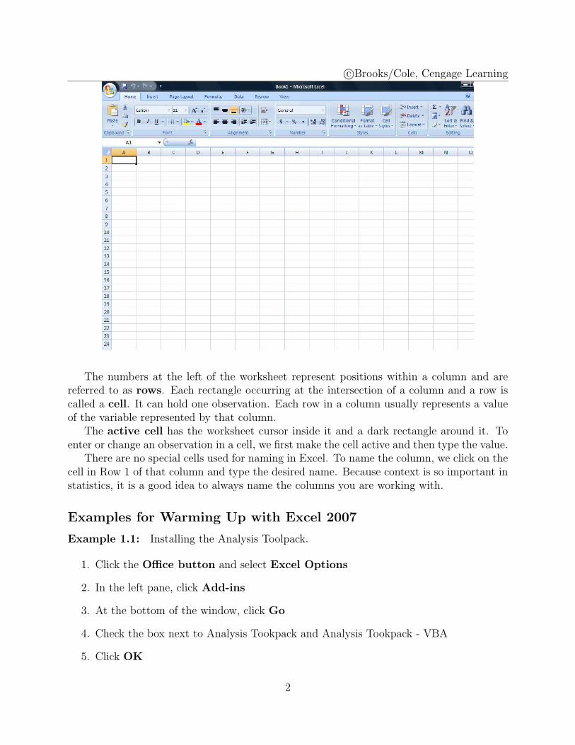
The numbers at the left of the worksheet represent positions within a column and arereferred to as rows. Each rectangle occurring at the intersection of a column and a row iscalled a cell. It can hold one observation. Each row in a column usually represents a valueof the variable represented by that column.

The active cell has the worksheet cursor inside it and a dark rectangle around it. Toenter or change an observation in a cell, we first make the cell active and then type the value.

There are no special cells used for naming in Excel. To name the column, we click on thecell in Row 1 of that column and type the desired name. Because context is so important instatistics, it is a good idea to always name the columns you are working with.

Examples for Warming Up with Excel 2007

Example 1.1: Installing the Analysis Toolpack.

1. Click the Office button and select Excel Options

2. In the left pane, click Add-ins

3. At the bottom of the window, click Go

4. Check the box next to Analysis Tookpack and Analysis Tookpack - VBA

5. Click OK

2


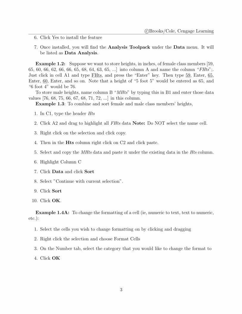
6. Click Yes to install the feature

7. Once installed, you will find the Analysis Toolpack under the Data menu. It willbe listed as Data Analysis.

Example 1.2: Suppose we want to store heights, in inches, of female class members [59,65, 60, 66, 62, 66, 66, 65, 68, 64, 63, 65, ...] into column A and name the column “FHts”;.Just click in cell A1 and type FHts, and press the “Enter” key. Then type 59, Enter, 65,Enter, 60, Enter, and so on. Note that a height of “5 foot 5” would be entered as 65, and“6 foot 4” would be 76.

To store male heights, name column B “MHts” by typing this in B1 and enter those datavalues [76, 68, 75, 66, 67, 68, 71, 72, ...] in this column.

Example 1.3: To combine and sort female and male class members’ heights,

1. In C1, type the header Hts

2. Click A2 and drag to highlight all FHts data Note: Do NOT select the name cell.

3. Right click on the selection and click copy.

4. Then in the Hts column right click on C2 and click paste.

5. Select and copy the MHts data and paste it under the existing data in the Hts column.

6. Highlight Column C

7. Click Data and click Sort

8. Select ”Continue with current selection”.

9. Click Sort

10. Click OK.

Example 1.4A: To change the formatting of a cell (ie, numeric to text, text to numeric,etc.):

1. Select the cells you wish to change formatting on by clicking and dragging

2. Right click the selection and choose Format Cells

3. On the Number tab, select the category that you would like to change the format to

4. Click OK

3


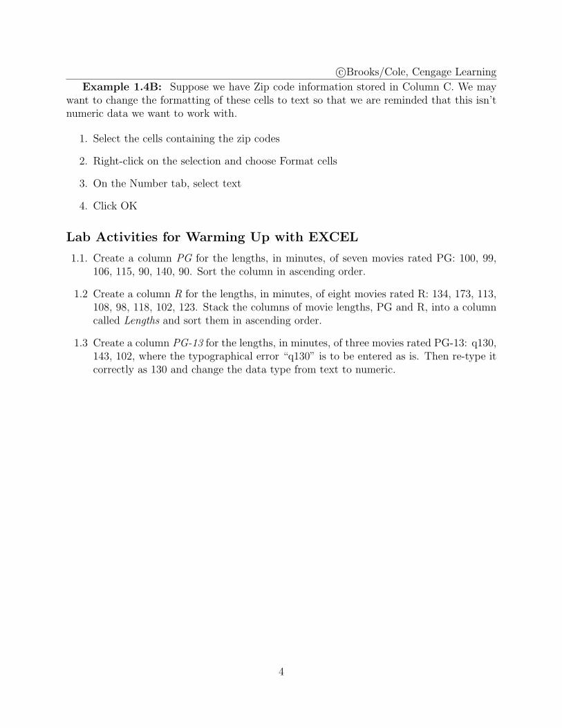
Example 1.4B: Suppose we have Zip code information stored in Column C. We maywant to change the formatting of these cells to text so that we are reminded that this isn’tnumeric data we want to work with.

1. Select the cells containing the zip codes

2. Right-click on the selection and choose Format cells

3. On the Number tab, select text

4. Click OK

Lab Activities for Warming Up with EXCEL

1.1. Create a column PG for the lengths, in minutes, of seven movies rated PG: 100, 99,106, 115, 90, 140, 90. Sort the column in ascending order.

1.2 Create a column R for the lengths, in minutes, of eight movies rated R: 134, 173, 113,108, 98, 118, 102, 123. Stack the columns of movie lengths, PG and R, into a columncalled Lengths and sort them in ascending order.

1.3 Create a column PG-13 for the lengths, in minutes, of three movies rated PG-13: q130,143, 102, where the typographical error “q130” is to be entered as is. Then re-type itcorrectly as 130 and change the data type from text to numeric.

4


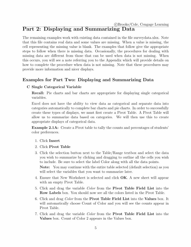
Part 2: Displaying and Summarizing Data

The remaining examples work with existing data contained in the file surveydata.xlsx. Notethat this file contains real data and some values are missing. When a value is missing, thecell representing the missing value is blank. The examples that follow give the appropriatesteps to follow when there is missing data. Occasionally, the procedures for dealing withmissing data are different from those that can be used when data is not missing. Whenthis occurs, you will see a note referring you to the Appendix which will provide details onhow to complete the procedure when data is not missing. Note that these procedures mayprovide more information and nicer displays.

Examples for Part Two: Displaying and Summarizing Data

C Single Categorical Variable

Recall: Pie charts and bar charts are appropriate for displaying single categoricalvariables.

Excel does not have the ability to view data as categorical and separate data intocategories automatically to complete bar charts and pie charts. In order to successfullycreate these types of displays, we must first create a Pivot Table. A Pivot Table willallow us to summarize data based on categories. We will then use this to createappropriate displays of categorical data.

Example 2.1A: Create a Pivot table to tally the counts and percentages of students’color preferences.

1. Click Insert

2. Click Pivot Table

3. Click the selection button next to the Table/Range textbox and select the datayou wish to summarize by clicking and dragging to outline all the cells you wishto include. Be sure to select the label Color along with all the data points.

Note: You may continue with the entire table selected (default selection) as youwill select the variables that you want to summarize later.

4. Ensure that New Worksheet is selected and click OK. A new sheet will appearwith an empty Pivot Table.

5. Click and drag the variable Color from the Pivot Table Field List into theRow Labels box. You should now see all the colors listed in the Pivot Table.

6. Click and drag Color from the Pivot Table Field List into the Values box. Itwill automatically choose Count of Color and you will see the counts appear inPivot Table.

7. Click and drag the variable Color from the Pivot Table Field List into theValues box. Count of Color 2 appears in the Values box.

5


8. Click the arrow next to Count of Color 2

9. Select Value Field Settings

10. Select the Show values as Tab

11. Under Show values as, select % of total from the drop down menu

12. Change the Custom name to % of total

13. Click OK

Example 2.1B: Create a pie chart for students’ color preferences.

1. First create a Pivot table with appropriate counts as above.

2. Click anywhere inside the Pivot table and click Insert

3. Click Pie and select Pie (the top left option). The pie chart will appear in a graphwindow.

Note: To edit the graph, you can use the PivotChart Tools submenu that appearsin the menu bar when the graph is selected. This submenu will allow you tocomplete tasks such as edit the titles, legends and overall appearance of the graph.

Example 2.1C: Create a bar chart for students’ color preferences.

1. First create a Pivot table with appropriate counts as above. Note: Do notinclude the % of total column in the Pivot Table, only include the Count ofColor.

2. Click anywhere inside the Pivot table and click Insert

3. Click Column and select Clustered column (the top left option). The bar chartwill appear in a graph window.

Note: If you choose Bar rather than Column, you will obtain the same graph,except the bars will be horizontal rather than vertical.

Q Single Quantitative Variable

Recall: Histograms and boxplots are appropriate display methods for single quanti-tative variables.

For a histogram (A), 5-number summary for a boxplot(B), and boxplot (C) of students’numbers of siblings,

Example 2.2A:

1. First click the tab to create a new sheet. We will store all our information forthe next few examples on the Sibs Data in this new worksheet. Double click thesheet name and type Sibs Data.

2. In cell A1 on the Sibs Data worksheet type Bins.

6


3. In cell A2 type 0, in cell A3 type 1, in cell A4 type 2, in cell A5 type 3, in cell A6type 4 and in cell A7 type 5

4. Click Data

5. Click Data Analysis

6. In the dialog box that pops up, select Histogram and click OK

7. Click the selection button in the textbox next to Input range. Click the surveydataworksheet tab and select the Sibs data Note: If you selected the label Sibs, youwill need to check the box next to Labels in Histogram dialog box, otherwise leavethe box unchecked.

8. Click the selection button in the textbox next to Bin Range. Click the Sibs Dataworksheet tab and select cells A1 through A7. Note: If you leave this textboxblank, Excel will automatically select bins for you.

9. Check the box next to Chart Output

10. Click OK

11. To remove the gaps, right-click a bar in the histogram

12. Click Format Data Series

13. Slide the gap width slider to No Gap

14. Click Close

Example 2.2B:

1. On the Sibs Data worksheet, select cell C1, type 5 number summary for Sibs, inC2 type Q1, in C3 type Min, in C4 type Median, in C5 type Max and in C6 typeQ3

2. Select D2 and click Formulas

3. Click Insert Function

4. Find and select QUARTILE and click OK

5. In the Array textbox, select the data for Sibs (click on the surveydata worksheettab then click and drag to select the data). (Note: Do not select the label Sibs.)In the Quart textbox, type 1 and click OK

6. Select D3 and click Insert Function

7. Find and select MIN and click OK

8. In the Number1 textbox, select the data for Sibs and click OK


10. Find and select MEDIAN and click OK


7



13. Find and select MAX and click OK



16. Find and select QUARTILE and click OK

17. In the Array textbox, select the data for Sibs. In the Quart textbox, type 3 andclick OK

Note: It is important to keep the 5 number summary in the order listed above. Failingto calculate the 5 number summary in this order will lead to problems producing aboxplot correctly.

Example 2.2C

1. Select the values you calculated in Example 2.2B and their labels. Note: Do notselect cell C1.

2. Click Insert

3. Click Line and select Line with Markers (1st column, 2nd row)

4. Click Switch Row/Column from the menu bar

5. Right click any data point and click Format Data Series

6. Click Line Color

7. Click No Line and click Close

8. While any data point is selected, click Layout from the submenu bar (at the topof the screen) for Chart Tools

9. Click Lines and select High-Low lines

10. Click Up/Down Bars and select Up/Down bars

11. Right click on the box and click Format Up Bars

12. Select No fill and click OK

Example 2.2D: This example produces mean, standard error for mean, median, mode,standard deviation, sample variance, kurtosis, skewness, range, minimum, maximum,sum, count, Q1 and Q3.

1. Click Data


3. Select Descriptive Statistics from Analysis Tools

4. Click OK

8


5. In the Input Range textbox, select the data for Sibs Note: If you selected thelabel Sibs, you will need to check the box next to Labels in Histogram dialog box,otherwise leave the box unchecked.

6. Check Summary statistics

7. Click OK

8. To add Q1 to the output, click the cell under Count and type Q1

9. Select the cell to the right of Q1 and click Formulas


11. Select QUARTILE from the list

12. In the Array textbox, select the data for Sibs. In the Quart textbox, type 1

13. Click OK

14. Under Q1, type Q3

15. Select the cell to the right of Q3 and click Formulas


17. Select QUARTILE from the list

18. In the Array textbox, select the data for Sibs. In the Quart textbox, type 3

19. Click OK

C→Q Relationship between Categorical Explanatory and Quantitative ResponseVariables

Recall: Side-by-side boxplots are an appropriate display for a categorical explanatoryvariable and a quantitative response variable.

Example 2.3A: (Paired design) To display and summarize the single sample of dif-ferences, ages of dads minus ages of moms, we first notice that these columns maycontain missing data. We do not want to summarize the pairs of data that are missingone or both of their values, so we will first need to create a list of differences for whichboth MomAge and DadAge are not missing

1. Create a new worksheet called MomDadAge Data

2. In A1 type Difference, in B1 type Missing and in C1 type Nonmissing Data

3. In A2 type =

4. Select the surveydata worksheet and select cell X2

5. Type -

6. Select the surveydata worksheet and select cell W2

7. Press Enter

8. Right click cell A2 and click copy

9


9. Select cells A3 through A447, right click and click paste

10. Select cell B2 and type =if(or(surveydata!X2=””, surveydata!W2=””), TRUE,FALSE)

11. Right click cell B2 and click copy

12. Select cells B3 through B447, right click and click paste

13. Select column B and click Data

14. Click Filter (an arrow appears in cell B1)

15. Click the arrow in cell B1 and uncheck the box next to TRUE

16. Click OK

17. Select all the data showing in column A (without selecting A1), right click andclick copy

18. Right click in the cell under Nonmissing Data and click paste

19. Click Filter

20. Right click in cell C2 (this cell should be empty) and click Delete

21. Select Shift cells up and click OK

22. Follow the procedure from Example 2.2A to create a histogram for the data incolumn C

Example 2.3B: (Two-sample design) To compare heights of students in the two gendergroups with summaries and a side-by-side boxplot,

1. Select the Female and Male Data worksheet

2. In H1 type Female and in I1 type Male

3. In G2 type Q1, in G3 type Min, in G4 type Median, in G5 type Max and in G6type Q3

4. Follow the procedure from Example 2.2B to find the 5 number summary for boththe female data (put these values in H2 through H6) and for the male data (putthese values in I2 through I6)

5. Select cells G1 through I6

6. Click Insert

7. Select Line and select Line with Markers

8. Click Switch Row/Column

9. For each line (5 total), right click on an endpoint and select Format Data Series

10. Click Line Color and select No Line then click Close

11. Click Layout and click Lines and select High-Low Lines

10


12. Click Up/Down bars and select Up/Down bars

13. Right click in one of the boxes and select Format Up bars

14. Select No fill

15. Click Close

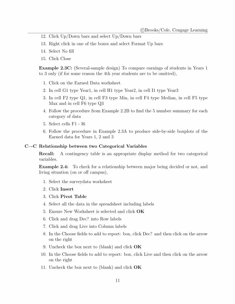
Example 2.3C: (Several-sample design) To compare earnings of students in Years 1to 3 only (if for some reason the 4th year students are to be omitted),

1. Click on the Earned Data worksheet

2. In cell G1 type Year1, in cell H1 type Year2, in cell I1 type Year3

3. In cell F2 type Q1, in cell F3 type Min, in cell F4 type Median, in cell F5 typeMax and in cell F6 type Q3

4. Follow the procedure from Example 2.2B to find the 5 number summary for eachcategory of data

5. Select cells F1 - I6

6. Follow the procedure in Example 2.3A to produce side-by-side boxplots of theEarned data for Years 1, 2 and 3

C→C Relationship between two Categorical Variables

Recall: A contingency table is an appropriate display method for two categoricalvariables.

Example 2.4: To check for a relationship between major being decided or not, andliving situation (on or off campus),

1. Select the surveydata worksheet

2. Click Insert

3. Click Pivot Table

4. Select all the data in the spreadsheet including labels

5. Ensure New Worksheet is selected and click OK

6. Click and drag Dec? into Row labels

7. Click and drag Live into Column labels

8. In the Choose fields to add to report: box, click Dec? and then click on the arrowon the right

9. Uncheck the box next to (blank) and click OK

10. In the Choose fields to add to report: box, click Live and then click on the arrowon the right

11. Uncheck the box next to (blank) and click OK

11


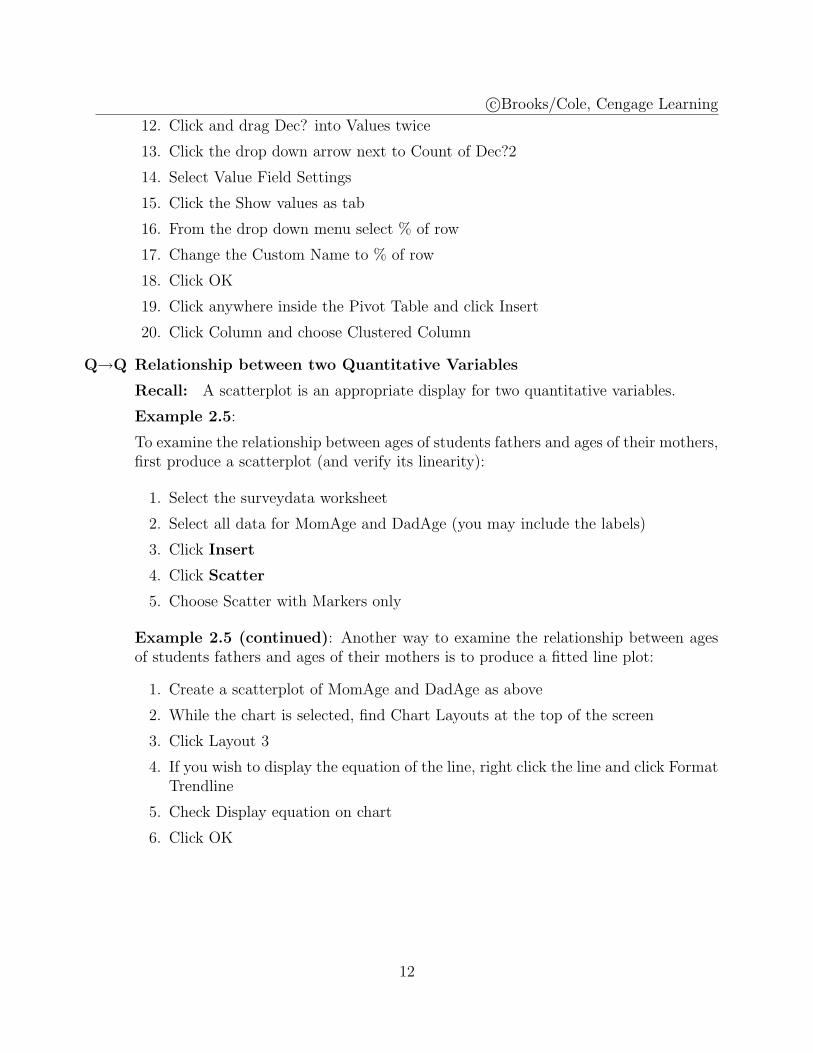
12. Click and drag Dec? into Values twice

13. Click the drop down arrow next to Count of Dec?2

14. Select Value Field Settings

15. Click the Show values as tab

16. From the drop down menu select % of row

17. Change the Custom Name to % of row

18. Click OK

19. Click anywhere inside the Pivot Table and click Insert

20. Click Column and choose Clustered Column

Q→Q Relationship between two Quantitative Variables

Recall: A scatterplot is an appropriate display for two quantitative variables.

Example 2.5:

To examine the relationship between ages of students fathers and ages of their mothers,first produce a scatterplot (and verify its linearity):

1. Select the surveydata worksheet

2. Select all data for MomAge and DadAge (you may include the labels)

3. Click Insert

4. Click Scatter

5. Choose Scatter with Markers only

Example 2.5 (continued): Another way to examine the relationship between agesof students fathers and ages of their mothers is to produce a fitted line plot:

1. Create a scatterplot of MomAge and DadAge as above

2. While the chart is selected, find Chart Layouts at the top of the screen

3. Click Layout 3

4. If you wish to display the equation of the line, right click the line and click FormatTrendline

5. Check Display equation on chart

6. Click OK

12


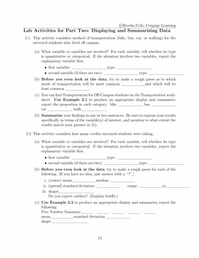
Lab Activities for Part Two: Displaying and Summarizing Data

2.1. This activity considers method of transportation (bike, bus, car, or walking) for thesurveyed students who lived off campus.

(a) What variable or variables are involved? For each variable, tell whether its typeis quantitative or categorical. If the situation involves two variables, report theexplanatory variable first.

• first variable: type:

• second variable (if there are two): type:

(b) Before you even look at the data, try to make a rough guess as to whichmode of transportation will be most common and which will beleast common .

(c) You can find Transportation for Off-Campus students on the Transportation work-sheet. Use Example 2.1 to produce an appropriate display and summaries;report the proportion in each category: bike , bus ,car , walk .

(d) Summarize your findings in one or two sentences. Be sure to express your resultsspecifically in terms of the variable(s) of interest, and mention to what extent theresults match your guesses in (b).

2.2 This activity considers how many credits surveyed students were taking.




(b) Before you even look at the data, try to make a rough guess for each of thefollowing: [If you have no idea, just answer with a “?”.]

i. (center) mean: median:

ii. (spread) standard deviation: range: to

iii. shape:Do you expect outliers? (Explain briefly.)

(c) Use Example 2.2 to produce an appropriate display and summaries; report thefollowing:Five Number Summary:mean standard deviationshape

13



2.3A For surveyed students, how does the number of minutes students spent exercising theday before compare with the number of minutes spent on the phone?

(a) In this situation, we should consider type of activity to be one variable, and timespent on the activity to be a second variable. For each of these variables, tellwhether it is quantitative or categorical, and whether its role is explanatory orresponse. Report the explanatory variable first:


• second variable: type:

(b) Before you even look at the data, try to make a reasonable guess for each ofthe following:

i. (center) Do you suspect the students spent more time exercising or on thephone? Do you think the sample of differences, time spent exercising minustime spent on the phone, will average out to a negative number, zero, or apositive number?

ii. (spread) Do you think the typical distance of the differences from their meanwill be just a few minutes or at least an hour?

iii. (shape) Do you expect the distribution of differences to be left-skewed orright-skewed? Do you expect outliers?

(c) Use Example 2.3A to produce an appropriate display and summaries to makea comparison:

i. On average, did the sampled students spend more time exercising or on thephone?

ii. Report and interpret the standard deviation of the time differences.

iii. Report and interpret the shape of the distribution of time differences.


2.3B For surveyed students, how do the shoe sizes of males compare to those of females?




14


(b) Before you even look at the data, try to make a reasonable guess for each ofthe following:

i. Which group will have a higher center (or about the same)?

ii. Which group will have more spread (or about the same)?

iii. What shapes do you expect?Do you expect outliers?

(c) Use Example 2.3B to produce an appropriate display and summaries to makea comparison:

i. Does one group have a considerably higher center?

ii. Does one group have more spread?

iii. Compare the shapes.


2.4 Does living on or off campus depend at all on whether a surveyed student is male orfemale?




(b) Before you even look at the data, do you expect the variables to be related?If so, for which explanatory group do you expect to see a higher proportion livingon campus?

(c) Use Example 2.4 to produce an appropriate display and summaries. Does onegroup have a considerably higher proportion living on campus?


2.5 How are surveyed students’ heights and weights related?




15


(b) Before you even look at the data, try to make a reasonable guess for each ofthe following: [If you have no idea, just answer with a “?”.]

i. form (linear or curved):

ii. direction (positive, negative, or none):

iii. strength (strong, moderate, or weak):Do you expect outliers or influential observations? (Explain briefly.)

(c) Use Example 2.5 to produce an appropriate display and summaries in order toanswer the following:Does the form appear roughly linear?What is the regression line equation?What is the value of the correlation r?What is the typical residual size s?


For more practice with techniques from this section, try these exercises from your text:Exercises 4.13 - 4.16, Exercises 4.41 - 4.45, Exercises 4.65 - 4.67, Exercises 4.85 - 4.86,Exercises 4.98 - 4.99, Exercises 5.84 - 5.90, Exercises 5.99 - 5.101, Exercises 5.115 - 5.119,Exercises 8.65 - 8.68, Exercises 8.80 - 8.83

16


Part 3: Probability

Examples for Part Three: Probability

Example 3.1 Generate a random sample of 10 heights from given data.

1. Select cell D449 and click Formulas


3. Find the RANDBETWEEN function and click OK

4. In the Bottom textbox, type 2

5. In the Top textbox, type 447 (the # of observations you have)

6. Click OK

7. Find the observation corresponding to the random number that appeared in the celland record it. This is your first observation in your random sample.

8. Continue this process until you have sampled 10 heights.

Note: In order to sample without replacement, if your RANDBETWEEN functionproduces the same number more than once during your sample, simply ignore it andtry again.

Lab Activities for Part Three: Probability

3.1 Use Example 3.1 to randomly sample (without replacement) 5 values from the col-umn Cash and report the total amount of cash carried by the five selected students.

3.2 The probability that at least two people in a group of 23 have the same birthday isapproximately 0.50; the probability that at least two people in a group of 60 have thesame birthday is approximately 0.99?

1. Use Example 3.1 to sample dates of the year, reprented by the numbers 1through 365.

2. Sample 23 dates with replacement, sort them, and check if there are duplicates.Take a total of twenty such samples with replacement, and report what proportioncontain duplicates: Is it close to 0.50?

3. Sample 60 dates with replacement, sort them, and check if there are duplicates.Take a total of twenty such samples with replacement, and report what proportioncontain duplicates: Is it close to 0.99?

17


Part 4: STATISTICAL INFERENCE

Examples for Part Four: Statistical Inference

C Single Categorical Variable

Recall: A Z-test is used when testing hypotheses about population proportions.

Example 4.1A: Use Excel to do inference about the population proportion of males/females;specifically, test if the sample represents a population with less than 40% males. In-cluding a display is a good habit to acquire in using software to perform inference.

1. Create a Pivot chart summarizing the counts of males and females

2. Create a Pie Chart from this Pivot table

3. In D3 (on the worksheet containing the Pivot table) type Sample size n then inE3 input the total number of observations (Grand total from Pivot table)

4. In D4 type successes and input the number of males E4

5. In D5 type Sample proportion and in E5 type =E4/E3

6. In the D6 Null hypothesis and type .4 in E6

7. In D7 type Standard error and type =sqrt((E6*(1-E6))/E3)

8. In D8 type Z test statistic and in E8 type = (E5-E6)/E7

9. In D9 type p-value

10. Select E9 and click Formulas then click Insert function

11. Find and select NORMDIST and click OK

12. In the X textbox, select E8, in the Mean textbox type 0, in the Standard devtextbox type 1, in the Cumulative textbox type TRUE

13. Click OK

Q Single Quantitative Variable

Recall: A Z-test is used to test hypotheses about a single population mean (orconstruct confidence intervals) when σ is known. A t-test is used to test hypothesesabout a population mean (or construct confidence intervals) when σ is unknown.

Example 4.2A: (σ known) Assume Verbal SAT scores of surveyed students to bea random sample taken from scores of all students at a particular university, whosemean score is unknown and standard deviation is 100. Use sample scores to obtaina 90% confidence interval for the unknown population mean score, after producing ahistogram of the scores.

1. Create a histogram as described above

2. Select cell C449 and click Formulas

18



4. Find and select AVERAGE

5. In the Number1 textbox, select the data for Verbal and click OK(Do not selectthe label.)

6. Select cell C450 and click Formulas

7. Click Insert function

8. Find and select CONFIDENCE and click OK

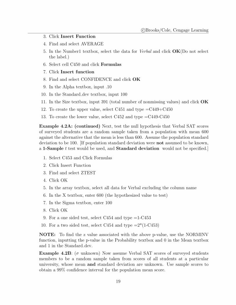
9. In the Alpha textbox, input .10

10. In the Standard dev textbox, input 100

11. In the Size textbox, input 391 (total number of nonmissing values) and click OK

12. To create the upper value, select C451 and type =C449+C450

13. To create the lower value, select C452 and type =C449-C450

Example 4.2A: (continued) Next, test the null hypothesis that Verbal SAT scoresof surveyed students are a random sample taken from a population with mean 600against the alternative that the mean is less than 600. Assume the population standarddeviation to be 100. [If population standard deviation were not assumed to be known,a 1-Sample t test would be used, and Standard deviation would not be specified.]

1. Select C453 and Click Formulas


3. Find and select ZTEST

4. Click OK

5. In the array textbox, select all data for Verbal excluding the column name

6. In the X textbox, enter 600 (the hypothesized value to test)

7. In the Sigma textbox, enter 100

8. Click OK

9. For a one sided test, select C454 and type =1-C453

10. For a two sided test, select C454 and type =2*(1-C453)

NOTE: To find the z value associated with the above p-value, use the NORMINVfunction, inputting the p-value in the Probability textbox and 0 in the Mean textboxand 1 in the Standard dev.

Example 4.2B: (σ unknown) Now assume Verbal SAT scores of surveyed studentsmembers to be a random sample taken from scores of all students at a particularuniversity, whose mean and standard deviation are unknown. Use sample scores toobtain a 99% confidence interval for the population mean score.

19


1. Select C455 and click Formulas


3. Find and select STDEV

4. Click OK

5. In the Number1 textbox, select the data for Verbal

6. Click OK

7. Select C456 and click Formulas


9. Find and select TINV

10. Click OK

11. In the Probability textbox, type .01

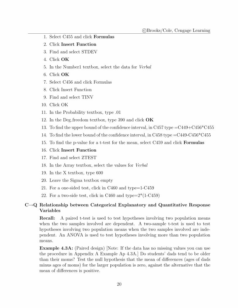
12. In the Deg freedom textbox, type 390 and click OK

13. To find the upper bound of the confidence interval, in C457 type =C449+C456*C455

14. To find the lower bound of the confidence interval, in C458 type =C449-C456*C455

15. To find the p-value for a t-test for the mean, select C459 and click Formulas


17. Find and select ZTEST

18. In the Array textbox, select the values for Verbal

19. In the X textbox, type 600

20. Leave the Sigma textbox empty

21. For a one-sided test, click in C460 and type=1-C459

22. For a two-side test, click in C460 and type=2*(1-C459)

C→Q Relationship between Categorical Explanatory and Quantitative ResponseVariables

Recall: A paired t-test is used to test hypotheses involving two population meanswhen the two samples involved are dependent. A two-sample t-test is used to testhypotheses involving two population means when the two samples involved are inde-pendent. An ANOVA is used to test hypotheses involving more than two populationmeans.

Example 4.3A: (Paired design) [Note: If the data has no missing values you can usethe procedure in Appendix A Example Ap 4.3A.] Do students’ dads tend to be olderthan their moms? Test the null hypothesis that the mean of differences (ages of dadsminus ages of moms) for the larger population is zero, against the alternative that themean of differences is positive.

20


1. Select C452, and click Formulas


3. Find and select TTEST

4. Click OK

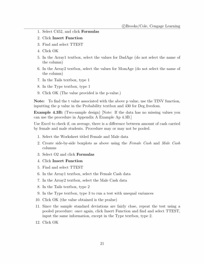
5. In the Array1 textbox, select the values for DadAge (do not select the name ofthe column)

6. In the Array2 textbox, select the values for MomAge (do not select the name ofthe column)

7. In the Tails textbox, type 1

8. In the Type textbox, type 1

9. Click OK (The value provided is the p-value.)

Note: To find the t value associated with the above p value, use the TINV function,inputting the p value in the Probability textbox and 430 for Deg freedom.

Example 4.3B: (Two-sample design) [Note: If the data has no missing values youcan use the procedure in Appendix A Example Ap 4.3B.]

Use Excel to check if, on average, there is a difference between amount of cash carriedby female and male students. Procedure may or may not be pooled.

1. Select the Worksheet titled Female and Male data

2. Create side-by-side boxplots as above using the Female Cash and Male Cashcolumns

3. Select O2 and click Formulas


5. Find and select TTEST

6. In the Array1 textbox, select the Female Cash data

7. In the Array2 textbox, select the Male Cash data

8. In the Tails textbox, type 2

9. In the Type textbox, type 3 to run a test with unequal variances

10. Click OK (the value obtained is the pvalue)

11. Since the sample standard deviations are fairly close, repeat the test using apooled procedure: once again, click Insert Function and find and select TTEST,input the same information, except in the Type textbox, type 2.

12. Click OK

21


Note: To find the t value associated with this p value, use the TINV function asabove.

Example 4.3C: (Several-sample design) Use Excel to see if there is a significantdifference in mean earnings of freshmen, sophomores, juniors, and seniors in the class.Include side-by-side boxplots to display the data.

1. Select the Earned Data worksheet

2. Click Data


4. Select Anova: Single Factor

5. Click OK

6. Select all the data excluding the labels

7. Click OK

C→C Relationship between two Categorical Variables

Recall: A χ2 test is used to determine if two categorical variables are independentor dependent.

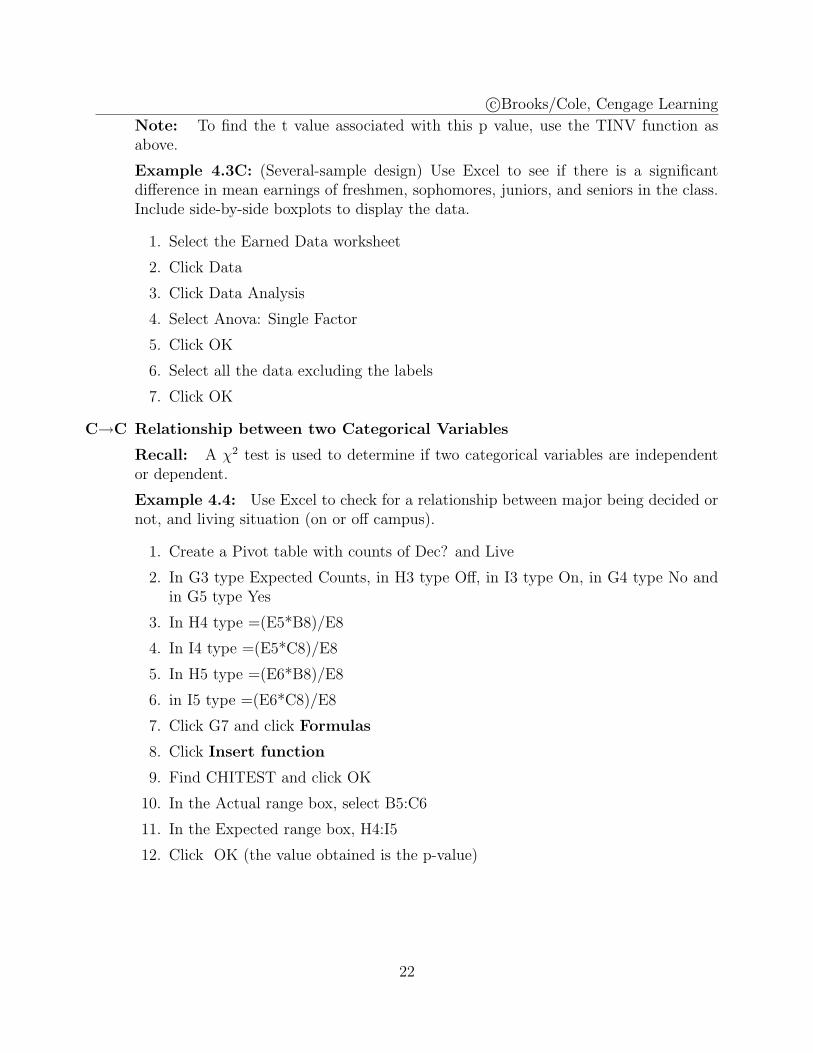
Example 4.4: Use Excel to check for a relationship between major being decided ornot, and living situation (on or off campus).

1. Create a Pivot table with counts of Dec? and Live

2. In G3 type Expected Counts, in H3 type Off, in I3 type On, in G4 type No andin G5 type Yes

3. In H4 type =(E5*B8)/E8

4. In I4 type =(E5*C8)/E8

5. In H5 type =(E6*B8)/E8

6. in I5 type =(E6*C8)/E8

7. Click G7 and click Formulas

8. Click Insert function

9. Find CHITEST and click OK

10. In the Actual range box, select B5:C6

11. In the Expected range box, H4:I5

12. Click OK (the value obtained is the p-value)

22


Q→Q Relationship between two Quantitative Variables

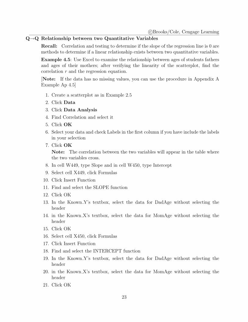
Recall: Correlation and testing to determine if the slope of the regression line is 0 aremethods to determine if a linear relationship exists between two quantitative variables.

Example 4.5: Use Excel to examine the relationship between ages of students fathersand ages of their mothers; after verifying the linearity of the scatterplot, find thecorrelation r and the regression equation.

[Note: If the data has no missing values, you can use the procedure in Appendix AExample Ap 4.5]

1. Create a scatterplot as in Example 2.5

2. Click Data


4. Find Correlation and select it

5. Click OK

6. Select your data and check Labels in the first column if you have include the labelsin your selection

7. Click OK

Note: The correlation between the two variables will appear in the table wherethe two variables cross.

8. In cell W449, type Slope and in cell W450, type Intercept

9. Select cell X449, click Formulas


11. Find and select the SLOPE function

12. Click OK

13. In the Known Y’s textbox, select the data for DadAge without selecting theheader

14. in the Known X’s textbox, select the data for MomAge without selecting theheader

15. Click OK

16. Select cell X450, click Formulas


18. Find and select the INTERCEPT function

19. In the Known Y’s textbox, select the data for DadAge without selecting theheader

20. in the Known X’s textbox, select the data for MomAge without selecting theheader

21. Click OK

23


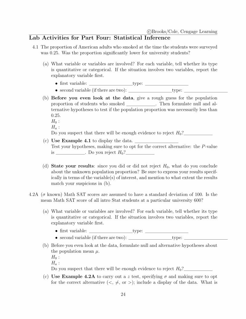
Lab Activities for Part Four: Statistical Inference

4.1 The proportion of American adults who smoked at the time the students were surveyedwas 0.25. Was the proportion significantly lower for university students?




(b) Before you even look at the data, give a rough guess for the populationproportion of students who smoked . Then formulate null and al-ternative hypotheses to test if the population proportion was necessarily less than0.25.H0 :Ha :Do you suspect that there will be enough evidence to reject H0?

(c) Use Example 4.1 to display the data.Test your hypotheses, making sure to opt for the correct alternative: the P -valueis . Do you reject H0?

(d) State your results: since you did or did not reject H0, what do you concludeabout the unknown population proportion? Be sure to express your results specif-ically in terms of the variable(s) of interest, and mention to what extent the resultsmatch your suspicions in (b).

4.2A (σ known) Math SAT scores are assumed to have a standard deviation of 100. Is themean Math SAT score of all intro Stat students at a particular university 600?




(b) Before you even look at the data, formulate null and alternative hypotheses aboutthe population mean µ.H0 :Ha :Do you suspect that there will be enough evidence to reject H0?

(c) Use Example 4.2A to carry out a z test, specifying σ and making sure to optfor the correct alternative (<, 6=, or >); include a display of the data. What is

24


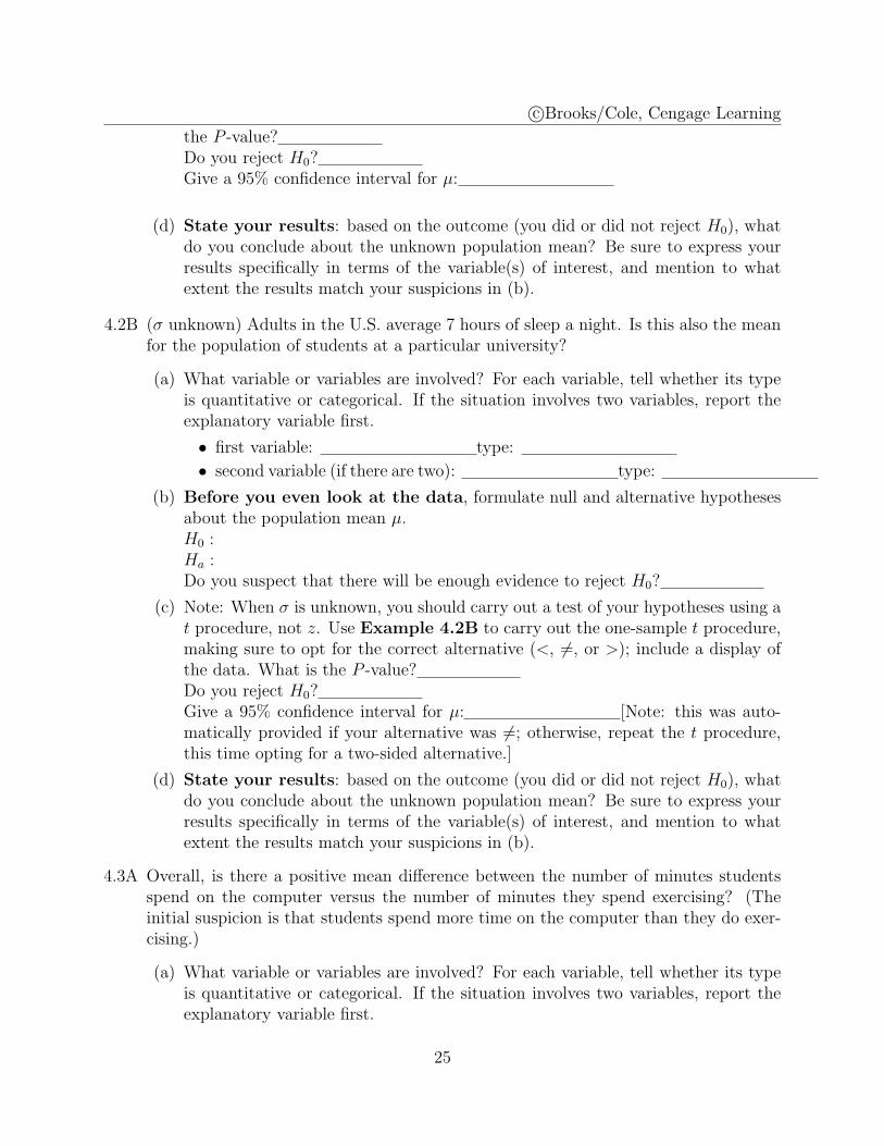
the P -value?Do you reject H0?Give a 95% confidence interval for µ:

(d) State your results: based on the outcome (you did or did not reject H0), whatdo you conclude about the unknown population mean? Be sure to express yourresults specifically in terms of the variable(s) of interest, and mention to whatextent the results match your suspicions in (b).

4.2B (σ unknown) Adults in the U.S. average 7 hours of sleep a night. Is this also the meanfor the population of students at a particular university?




(b) Before you even look at the data, formulate null and alternative hypothesesabout the population mean µ.H0 :Ha :Do you suspect that there will be enough evidence to reject H0?

(c) Note: When σ is unknown, you should carry out a test of your hypotheses using at procedure, not z. Use Example 4.2B to carry out the one-sample t procedure,making sure to opt for the correct alternative (<, 6=, or >); include a display ofthe data. What is the P -value?Do you reject H0?Give a 95% confidence interval for µ: [Note: this was auto-matically provided if your alternative was 6=; otherwise, repeat the t procedure,this time opting for a two-sided alternative.]

(d) State your results: based on the outcome (you did or did not reject H0), whatdo you conclude about the unknown population mean? Be sure to express yourresults specifically in terms of the variable(s) of interest, and mention to whatextent the results match your suspicions in (b).

4.3A Overall, is there a positive mean difference between the number of minutes studentsspend on the computer versus the number of minutes they spend exercising? (Theinitial suspicion is that students spend more time on the computer than they do exer-cising.)


25




(b) Before you even look at the data, formulate null and alternative hypothesesabout the population mean difference µd.H0 :Ha :Do you suspect that there will be enough evidence to reject H0?

(c) Use Example 4.3A to carry out a paired t procedure, making sure to opt forthe correct alternative (<, 6=, or >); include a display of the data. What is theP -value?Do you reject H0?

(d) State your results: based on the outcome (you did or did not rejectH0), what doyou conclude about the unknown population mean difference? Be sure to expressyour results specifically in terms of the variable(s) of interest, and mention towhat extent the results match your suspicions in (b).

4.3B Is the mean number of credits taken the same for all on- and off-campus students at aparticular university?




(b) Before you even look at the data, formulate null and alternative hypothesesabout the difference µ1 − µ2 between population means for the two groups. [Thenull hypothesis usually states that this difference is zero.]H0 :Ha :Do you suspect that there will be enough evidence to reject H0?

(c) Use Example 4.3B to carry out a two-sample t procedure, making sure to optfor the correct alternative (<, 6=, or >); include a display of the data. What isthe P -value?Do you reject H0?

(d) State your results: based on the outcome (you did or did not reject H0), whatdo you conclude about the unknown difference between population means? Besure to express your results specifically in terms of the variable(s) of interest, andmention to what extent the results match your suspicions in (b).

26


4.3C In general, is mean age the same for students who wear contact lenses, glasses, orneither?




(b) Before you even look at the data, formulate null and alternative hypothesesabout the population means.H0 :Ha :Do you suspect that there will be enough evidence to reject H0?

(c) Use Example 4.3C to carry out an ANOVA procedure; include a display of thedata. What is the P -value?Do you reject H0?

(d) State your results: based on the outcome (you did or did not reject H0), whatdo you conclude about the various population means? Be sure to express yourresults specifically in terms of the variable(s) of interest, and mention to whatextent the results match your suspicions in (b).

4.4 Is there a statistically significant relationship between whether or not a student smokesand whether the student lives on or off campus?




(b) Before you even look at the data, formulate null and alternative hypothesesabout the relationship between those variables.H0 :Ha :Do you suspect that there will be enough evidence to reject H0?

(c) Use Example 4.4 to construct a two-way table of counts and row percents,and carry out a chi-square test; include a display of the data. What is the P -value?Do you reject H0?

27


(d) State your results: based on the outcome (you did or did not reject H0), doyou conclude that those variables are related? Be sure to express your resultsspecifically in terms of the variable(s) of interest, and mention to what extent theresults match your suspicions in (b).

4.5 Is there a relationship between the heights of students’ fathers and mothers?




(b) Before you even look at the data, formulate null and alternative hypothesesabout the slope β1 of the population regression line.H0 :Ha :Do you suspect that there will be enough evidence to reject H0?

(c) Use Example 4.5 to display the data and verify that the form is reasonablylinear. Then carry out a regression procedure to test your hypotheses. What isthe P -value?Do you reject H0?

(d) State your results: based on the outcome (you did or did not reject H0), doyou conclude that the population variables are related? Be sure to express yourresults specifically in terms of the variable(s) of interest, and mention to whatextent the results match your suspicions in (b).

For more practice with techniques from this section, try these exercises from your text:Exercises 9.32 - 9.35, Exercises 9.68 - 9.71, Exercises 9.93 - 9.95, Exercises 10.73 -10.85,

Exercises 11.50 - 11.51, Exercises 11.70 - 11.73, Exercises 11.80 - 11.103, Exercises 12.44 -12.54, Exercises 13.50 - 13.58

28


1 Appendix A

Example Ap 4.3A To complete a t-test for paired samples:

1. Click Data


3. Select t-Test: Paired Two Sample for Means

4. Click OK

5. In the Variable 1 Range textbox, select the data for the first sample

6. In the Variable 2 Range textbox, select the data for the second sample

7. In the Hypothesized Mean Difference type the value to be tested

8. In the Alpha textbox, type the appropriate value for the significance level

9. Click OK

Return to Example 4.3A

Example Ap 4.3B To complete a two sample t-test assuming equal variances (unequalvariances):

1. Click Data


3. Select t-Test: Two-Sample Assuming Equal Variances (Unequal Variances)

4. Click OK

5. In the Variable 1 Range textbox, select the data for the first sample Note: If youselected the label for the data, you will need to check the box next to Labels inHistogram dialog box, otherwise leave the box unchecked.

6. In the Variable 2 Range textbox, select the data for the second sample Note: Ifyou selected the label for the data, you will need to check the box next to Labels inHistogram dialog box, otherwise leave the box unchecked.

7. In the Hypothesized Mean Difference type the value to be tested

8. In the Alpha textbox, type the appropriate value for the significance level

9. Click OK

29


Return to Example 4.3B

Example Ap 4.5To examine the relationship between two quantitative variables by producing the regres-

sion equation:

1. Click Data


3. Select Regression

4. Click OK

5. In the textbox for Input Y Range, select the response (dependent) variable

6. In the textbox for Input X range, select the explanatory (independent) variable

7. Check the box next to Residuals

8. Click OK

Return to Example 4.5

30

Documents

Excel 2007 BASICS for Elementary Statistics: Looking at the Big