Embed Size (px)
Citation preview
Examining the Effects of Site Selection Criteria for Evaluating the Effectiveness of Traffic Safety Countermeasures
Dominique Lord* Associate Professor and Zachry Development Professor I
Zachry Department of Civil Engineering Texas A&M University
3136 TAMU College Station, TX 77843-3136
Tel. (979) 458-3949 Fax. (979) 845-6481
Email: [email protected]
Pei-Fen Kuo Research Assistant
Zachry Department of Civil Engineering Texas A&M University
3136 TAMU College Station, TX 77843-3136
Tel. (979) 862-3446 Fax. (979) 845-6481
Email: [email protected]
November 20, 2011
Revised Version
Paper accepted for publication in AA&P
*Corresponding Author
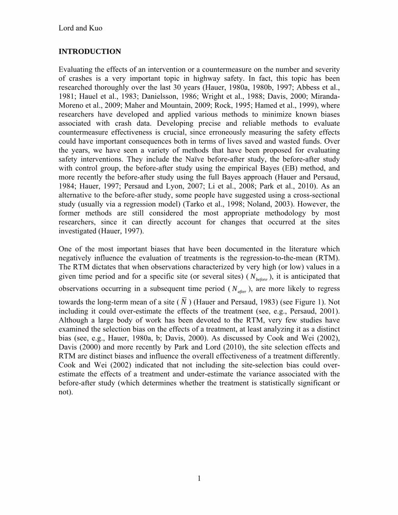
ABSTRACT The primary objective of this paper is to describe how site selection effects can influence the safety effectiveness of treatments. More specifically, the goal is to quantify the bias for the safety effectiveness of a treatment as a function of different entry criteria as well as other factors associated with crash data, and propose a new method to minimize this bias when a control group is not available. The study objective was accomplished using simulated data. The proposed method documented in this paper was compared to the four most common types of before-after studies: the Naïve, using a control group (CG), the empirical Bayes (EB) method based on the method of moment (EBMM), and the EB method based on a control group (EBCG). Five scenarios were examined: a direct comparison of the methods, different dispersion parameter values of the Negative Binomial model, different sample sizes, different values of the index of safety effectiveness ( ), and different levels of uncertainty associated with the index. Based on the simulated scenarios (also supported theoretically), the study results showed that higher entry criteria, larger values of the safety effectiveness, and smaller dispersion parameter values will cause a larger selection bias. Furthermore, among all methods evaluated, the Naïve and the EBMM methods are both significantly affected by the selection bias. Using a control group, or the EBCG, can mutually eliminate the site selection bias, as long as the characteristics of the control group (truncated data for the CG method or the non-truncated sample population for the EBCG method) are exactly the same as for the treatment group. In practice, finding datasets for the control group with the exact same characteristics as for the treatment group may not always be feasible. To overcome this problem, the method proposed in this study can be used to adjust the naïve estimator of the index of safety effectiveness, even when the mean and dispersion parameter are not properly estimated. Key words: regression-to-the-mean, biased estimate, safety index, site selection effects, before-after study, Empirical Bayes Method
Lord and Kuo
1
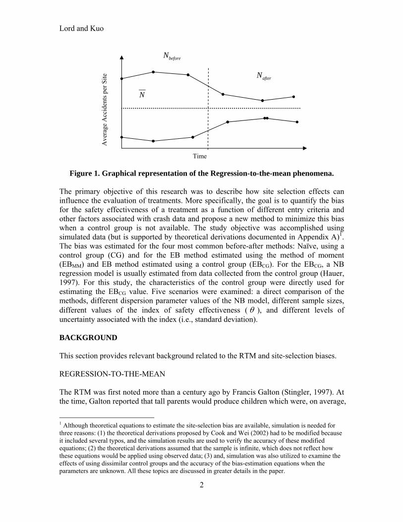
INTRODUCTION Evaluating the effects of an intervention or a countermeasure on the number and severity of crashes is a very important topic in highway safety. In fact, this topic has been researched thoroughly over the last 30 years (Hauer, 1980a, 1980b, 1997; Abbess et al., 1981; Hauel et al., 1983; Danielsson, 1986; Wright et al., 1988; Davis, 2000; Miranda-Moreno et al., 2009; Maher and Mountain, 2009; Rock, 1995; Hamed et al., 1999), where researchers have developed and applied various methods to minimize known biases associated with crash data. Developing precise and reliable methods to evaluate countermeasure effectiveness is crucial, since erroneously measuring the safety effects could have important consequences both in terms of lives saved and wasted funds. Over the years, we have seen a variety of methods that have been proposed for evaluating safety interventions. They include the Naïve before-after study, the before-after study with control group, the before-after study using the empirical Bayes (EB) method, and more recently the before-after study using the full Bayes approach (Hauer and Persaud, 1984; Hauer, 1997; Persaud and Lyon, 2007; Li et al., 2008; Park et al., 2010). As an alternative to the before-after study, some people have suggested using a cross-sectional study (usually via a regression model) (Tarko et al., 1998; Noland, 2003). However, the former methods are still considered the most appropriate methodology by most researchers, since it can directly account for changes that occurred at the sites investigated (Hauer, 1997). One of the most important biases that have been documented in the literature which negatively influence the evaluation of treatments is the regression-to-the-mean (RTM). The RTM dictates that when observations characterized by very high (or low) values in a given time period and for a specific site (or several sites) ( beforeN ), it is anticipated that
observations occurring in a subsequent time period ( afterN ), are more likely to regress
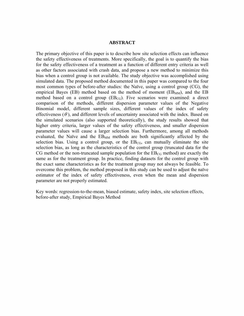
towards the long-term mean of a site ( N ) (Hauer and Persaud, 1983) (see Figure 1). Not including it could over-estimate the effects of the treatment (see, e.g., Persaud, 2001). Although a large body of work has been devoted to the RTM, very few studies have examined the selection bias on the effects of a treatment, at least analyzing it as a distinct bias (see, e.g., Hauer, 1980a, b; Davis, 2000). As discussed by Cook and Wei (2002), Davis (2000) and more recently by Park and Lord (2010), the site selection effects and RTM are distinct biases and influence the overall effectiveness of a treatment differently. Cook and Wei (2002) indicated that not including the site-selection bias could over-estimate the effects of a treatment and under-estimate the variance associated with the before-after study (which determines whether the treatment is statistically significant or not).
Lord and Kuo
2
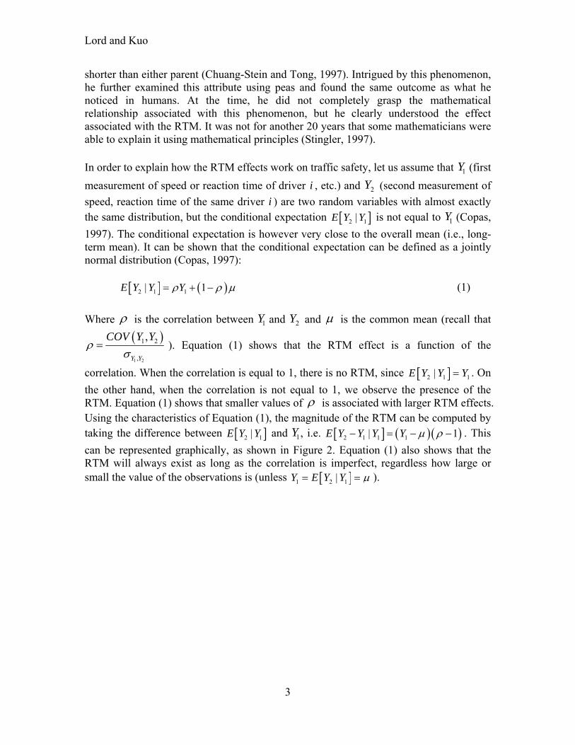
Figure 1. Graphical representation of the Regression-to-the-mean phenomena.
The primary objective of this research was to describe how site selection effects can influence the evaluation of treatments. More specifically, the goal is to quantify the bias for the safety effectiveness of a treatment as a function of different entry criteria and other factors associated with crash data and propose a new method to minimize this bias when a control group is not available. The study objective was accomplished using simulated data (but is supported by theoretical derivations documented in Appendix A)1. The bias was estimated for the four most common before-after methods: Naïve, using a control group (CG) and for the EB method estimated using the method of moment (EBMM) and EB method estimated using a control group (EBCG). For the EBCG, a NB regression model is usually estimated from data collected from the control group (Hauer, 1997). For this study, the characteristics of the control group were directly used for estimating the EBCG value. Five scenarios were examined: a direct comparison of the methods, different dispersion parameter values of the NB model, different sample sizes, different values of the index of safety effectiveness ( ), and different levels of uncertainty associated with the index (i.e., standard deviation). BACKGROUND This section provides relevant background related to the RTM and site-selection biases. REGRESSION-TO-THE-MEAN The RTM was first noted more than a century ago by Francis Galton (Stingler, 1997). At the time, Galton reported that tall parents would produce children which were, on average,
1 Although theoretical equations to estimate the site-selection bias are available, simulation is needed for three reasons: (1) the theoretical derivations proposed by Cook and Wei (2002) had to be modified because it included several typos, and the simulation results are used to verify the accuracy of these modified equations; (2) the theoretical derivations assumed that the sample is infinite, which does not reflect how these equations would be applied using observed data; (3) and, simulation was also utilized to examine the effects of using dissimilar control groups and the accuracy of the bias-estimation equations when the parameters are unknown. All these topics are discussed in greater details in the paper.
N
beforeN
afterN
Time
Ave
rage
Acc
iden
ts p
er S
ite
Lord and Kuo
3
shorter than either parent (Chuang-Stein and Tong, 1997). Intrigued by this phenomenon, he further examined this attribute using peas and found the same outcome as what he noticed in humans. At the time, he did not completely grasp the mathematical relationship associated with this phenomenon, but he clearly understood the effect associated with the RTM. It was not for another 20 years that some mathematicians were able to explain it using mathematical principles (Stingler, 1997). In order to explain how the RTM effects work on traffic safety, let us assume that 1Y (first
measurement of speed or reaction time of driver i , etc.) and 2Y (second measurement of
speed, reaction time of the same driver i ) are two random variables with almost exactly the same distribution, but the conditional expectation 2 1|E Y Y is not equal to 1Y (Copas,
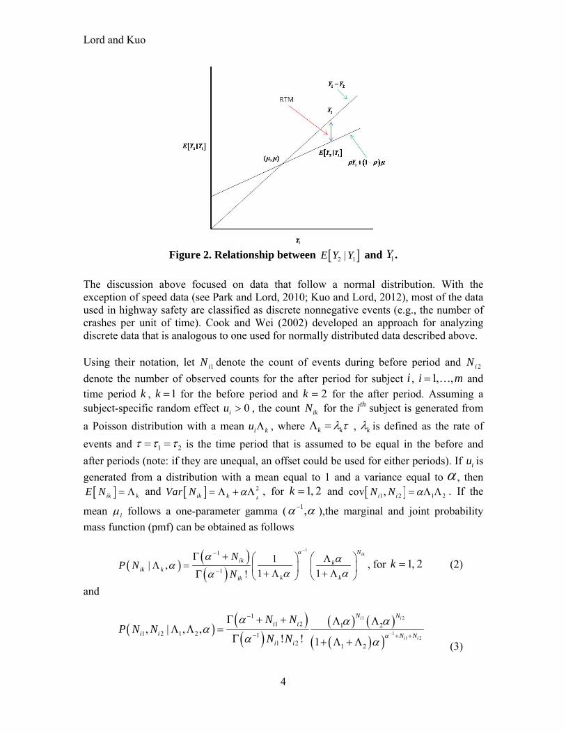
1997). The conditional expectation is however very close to the overall mean (i.e., long-term mean). It can be shown that the conditional expectation can be defined as a jointly normal distribution (Copas, 1997): 2 1 1| 1E Y Y Y (1)
Where is the correlation between 1Y and 2Y and is the common mean (recall that
1 2
1 2
,
,
Y Y
COV Y Y
). Equation (1) shows that the RTM effect is a function of the
correlation. When the correlation is equal to 1, there is no RTM, since 2 1 1|E Y Y Y . On
the other hand, when the correlation is not equal to 1, we observe the presence of the RTM. Equation (1) shows that smaller values of is associated with larger RTM effects. Using the characteristics of Equation (1), the magnitude of the RTM can be computed by taking the difference between 2 1|E Y Y and 1Y , i.e. 2 1 1 1| 1E Y Y Y Y . This
can be represented graphically, as shown in Figure 2. Equation (1) also shows that the RTM will always exist as long as the correlation is imperfect, regardless how large or small the value of the observations is (unless 1 2 1|Y E Y Y ).
Lord and Kuo
4
Figure 2. Relationship between 2 1|E Y Y and 1Y .
The discussion above focused on data that follow a normal distribution. With the exception of speed data (see Park and Lord, 2010; Kuo and Lord, 2012), most of the data used in highway safety are classified as discrete nonnegative events (e.g., the number of crashes per unit of time). Cook and Wei (2002) developed an approach for analyzing discrete data that is analogous to one used for normally distributed data described above. Using their notation, let 1iN denote the count of events during before period and 2iN
denote the number of observed counts for the after period for subject i , 1, ,i m and time period k , 1k for the before period and 2k for the after period. Assuming a subject-specific random effect 0iu , the count ikN for the ith subject is generated from
a Poisson distribution with a mean i ku , where k k , k is defined as the rate of
events and 1 2 is the time period that is assumed to be equal in the before and
after periods (note: if they are unequal, an offset could be used for either periods). If iu is
generated from a distribution with a mean equal to 1 and a variance equal to , then ik kE N and 2
kik kVar N , for 1, 2k and 1 2 1 2cov ,i iN N . If the
mean i follows a one-parameter gamma ( 1, ),the marginal and joint probability
mass function (pmf) can be obtained as follows
11
1
1| ,
1 1!
ikNik k
ik kk kik
NP N
N
, for 1, 2k (2)
and
1 2
11 2
11 2 1 2
1 2 1 2 11 2 1 2
, | , ,! ! 1
i i
i i
N Ni i
i i N Ni i
N NP N N
N N
(3)
Lord and Kuo
5
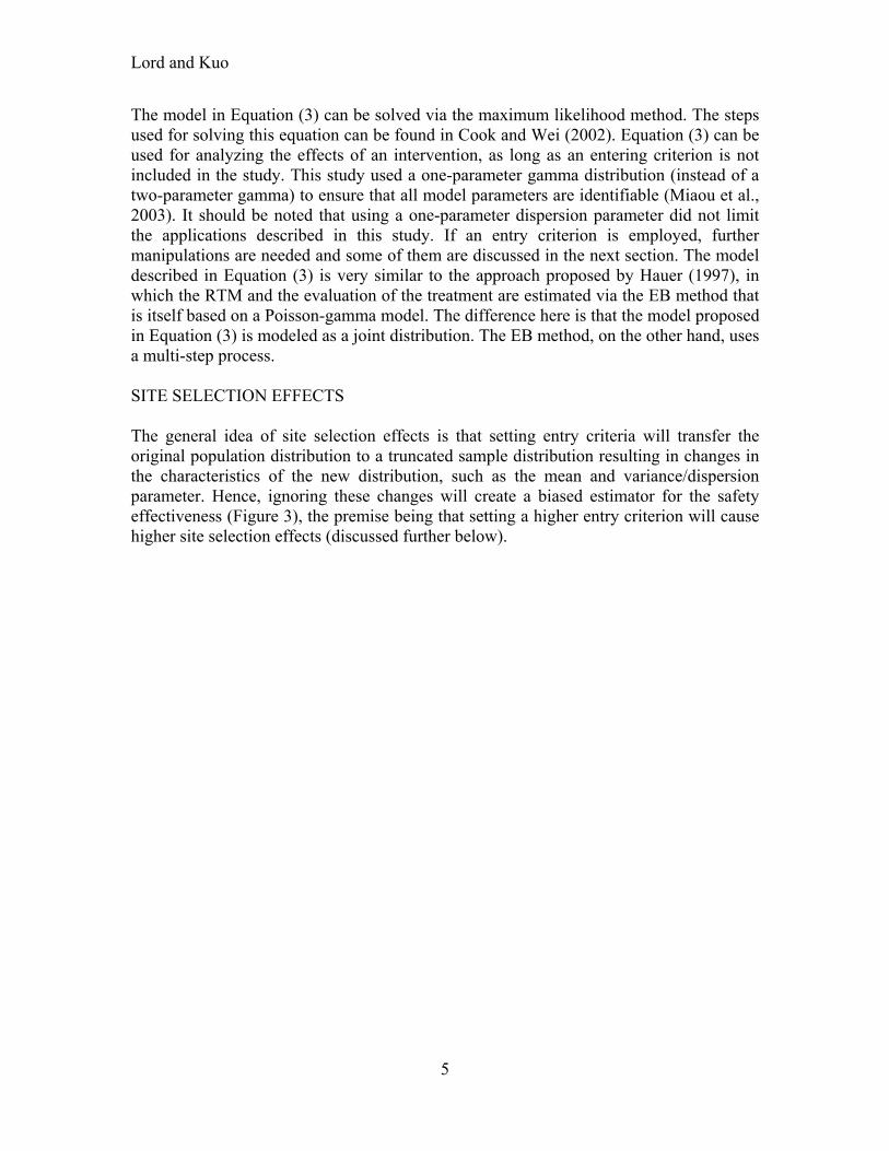
The model in Equation (3) can be solved via the maximum likelihood method. The steps used for solving this equation can be found in Cook and Wei (2002). Equation (3) can be used for analyzing the effects of an intervention, as long as an entering criterion is not included in the study. This study used a one-parameter gamma distribution (instead of a two-parameter gamma) to ensure that all model parameters are identifiable (Miaou et al., 2003). It should be noted that using a one-parameter dispersion parameter did not limit the applications described in this study. If an entry criterion is employed, further manipulations are needed and some of them are discussed in the next section. The model described in Equation (3) is very similar to the approach proposed by Hauer (1997), in which the RTM and the evaluation of the treatment are estimated via the EB method that is itself based on a Poisson-gamma model. The difference here is that the model proposed in Equation (3) is modeled as a joint distribution. The EB method, on the other hand, uses a multi-step process. SITE SELECTION EFFECTS The general idea of site selection effects is that setting entry criteria will transfer the original population distribution to a truncated sample distribution resulting in changes in the characteristics of the new distribution, such as the mean and variance/dispersion parameter. Hence, ignoring these changes will create a biased estimator for the safety effectiveness (Figure 3), the premise being that setting a higher entry criterion will cause higher site selection effects (discussed further below).
Lord and Kuo
6
Figure 3. The population distribution for complete and truncated sample.
When selecting sites for treatment, transportation agencies can select these sites based on a required minimum the number of crashes. For instance, Warrant 7 that is used for justifying the installation of traffic signals base solely on safety in the Manual on Uniform Traffic Control Device (MUTCD) states that a site must experience five or more failure-to-yield crashes within a 12-month period (FHWA, 2010). Hence, when such traffic signals are evaluated to address a safety problem, the sample should theoretically be extracted from sites that met Warrant 7 of the MUTCD. Setting a minimum entry criterion is not limited to practitioners, as researchers have also used entry criteria for evaluating safety projects (Miranda-Moreno et al., 2009). Furthermore, in many other cases, the selection effect exists but is never explicitly spelled out, because the safety evaluation of a treatment often includes sites that are greater than 0, even if the sites selected for treatment were not chosen specifically for safety reasons. When the entry criterion is small, say when all the sites experience at least one crash (Ni1> 0), there is a bias, as explained further below. Unlike the extensive discussions related to the RTM, estimating the magnitude of the site selection effects directly by their entry criteria values is a relatively new topic in traffic safety. As discussed above, selection bias has been sporadically studied over the last thirty years ago (Hauer, 1980a,b; Abbess et al., 1981; Davis, 2000), but has not been
Lord and Kuo
7
explicitly incorporated into the evaluation of treatments, at least not as a distinct effect as the one attributed to the RTM, with one exception. Using the work of Rubin (1977) and Pearl (2009) among others, Davis (2000) discussed how site selection effects could influence the estimation of a treatment by assigning probabilities to sites that have zero or more than zero observations (C=0)2. The primary method proposed by Davis does not specifically include an entry criterion variable for different values, which means that the bias cannot be directly estimated by the value of entry criterion, as it is done in this paper. Furthermore, the estimator based on Rubin’s work requires extra information, such as the need for collecting data for the control group, which is not needed for the approach proposed in this paper (although it may be useful to collect and include such data for improving the estimates of the safety effects of a treatment). The use of entry criteria in before-after studies, however, has been commonly adopted in other areas, especially in medical studies (e.g., clinical trials). Cook and Wei (2002), for instance, discussed the possible impacts of the selection effects for testing new medicines in clinical studies and derived the mathematical equations to account for the bias created by setting an entry criterion. They developed the methodology for data that follow a normal distribution and for count data. Their most important findings included the following:
1. Normally distributed responses: when scientists set the entry criteria for choosing experiment subjects, the original unbiased estimators of treatment effectiveness become biased. Even when there is no any relationship between the response in the before and after periods, 0 , the analysis can be biased. Furthermore, when the treatment does not work, using the naïve before-after method may lead to a positive estimate of treatment effectiveness, especially for low value responses. The selection bias will exist until the correlation (ρ) is 1 or the entry criteria (C) tend to -∞ (see Equation (4)). However, when a control group with the exact same characteristics is used in the before-after study, the biases related to the RTM and site selection will cancel out.
2
1
1| , 1, ,
f dE Y C i m
F d
(4)
Where, 2 1 2 1Y Y is an unbiased estimator of 2 1 ; 1iY and 2iY
are the response variables before ( 1k ) and after ( 2k ) the treatment, for
subject, 1, ,i m ; ik k i ikY u with ~ 0,iu N and 2~ 0,ik N ;
2 Pearl (2009) derived useful boundary equations for describing possible casual effects for the evaluation of treatments. However, there are several limitations about applying Pearl’s equations in traffic safety. They include (1) the boundaries only show the probability of that the event happened instead of actual impact value, (2) the boundaries are too wide to compare treatments, (3) the definitions of event that happened are subjective, and (4) very detailed information are necessary to compute the effects of a treatment. Due to space constraints, these issues are not discussed here, but the curious reader is referred to Kuo (2012) for additional discussion about these limitations.
Lord and Kuo
8
k k ikiY Y m is an unbiased estimate of k ; 2 , 0 is the
correlation between time period 1k and 2k ; 21d c ; and,
f d and 1F d F d are the density and CDF is the standard normal
distribution.
2. Count data responses: The results are analogous as for the Normal Distribution response. The bias for estimating the treatment performance increased when setting higher entry criteria, but the bias always exist until the entry criteria is less than 0 (C<0). Details about the mathematical equations are presented in the next section.
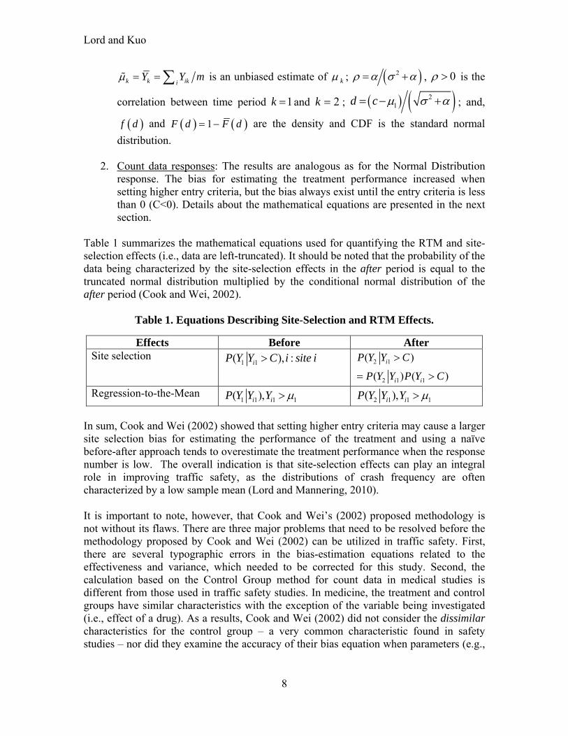
Table 1 summarizes the mathematical equations used for quantifying the RTM and site-selection effects (i.e., data are left-truncated). It should be noted that the probability of the data being characterized by the site-selection effects in the after period is equal to the truncated normal distribution multiplied by the conditional normal distribution of the after period (Cook and Wei, 2002).
Table 1. Equations Describing Site-Selection and RTM Effects.
Effects Before After Site selection
1 1( ), :iP Y Y C i site i 2 1
2 1 1
( )
( ) ( )
i
i i
P Y Y C
P Y Y P Y C
Regression-to-the-Mean 1 1 1 1( ),i iP Y Y Y 2 1 1 1( ),i iP Y Y Y
In sum, Cook and Wei (2002) showed that setting higher entry criteria may cause a larger site selection bias for estimating the performance of the treatment and using a naïve before-after approach tends to overestimate the treatment performance when the response number is low. The overall indication is that site-selection effects can play an integral role in improving traffic safety, as the distributions of crash frequency are often characterized by a low sample mean (Lord and Mannering, 2010). It is important to note, however, that Cook and Wei’s (2002) proposed methodology is not without its flaws. There are three major problems that need to be resolved before the methodology proposed by Cook and Wei (2002) can be utilized in traffic safety. First, there are several typographic errors in the bias-estimation equations related to the effectiveness and variance, which needed to be corrected for this study. Second, the calculation based on the Control Group method for count data in medical studies is different from those used in traffic safety studies. In medicine, the treatment and control groups have similar characteristics with the exception of the variable being investigated (i.e., effect of a drug). As a results, Cook and Wei (2002) did not consider the dissimilar characteristics for the control group – a very common characteristic found in safety studies – nor did they examine the accuracy of their bias equation when parameters (e.g.,
Lord and Kuo
9
1, , ) are unknown. To these ends, the following sections show the updated equation
for estimating the bias caused by the setting an entry criterion. COMPUTATION OF SITE SELECTION BIAS This section describes the methodology used for estimating the selection biased for count data. As discussed above, some of the equations shown further below have been revised, since the original ones described in the paper by Cook and Wei (2002) contained several typographical errors related to the estimators of parameters. Thus, to ensure a complete description, all the equations are reproduced in this paper. ESTIMATOR OF θ WITH ENTRY CRITERIA Suppose that site i (i=1, 2,…, m) experience 1iN crashes during the before period (time
length = t1) and 2iN crashes in the after period (time length = t2). Let ikN follow the
Poisson distribution ( ikN ~ Poisson ( i ku )), where is a subject-specific random effect,
and is the average crash rate ( k i kt ). The term refers to the instant rate of
crash. Let 2 1 , often defined as the index of safety effectiveness (Persaud and Lyon,
2007), and 2 1 , the difference in the number of crashes; for this paper, we will
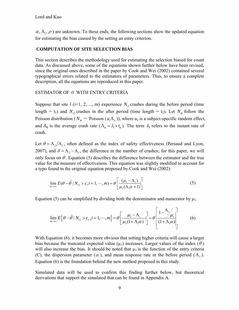
only focus on . Equation (5) describes the difference between the estimator and the true value for the measure of effectiveness. This equation was slightly modified to account for a typo found in the original equation proposed by Cook and Wei (2002):
1 11
1 1
( )ˆlim ( | , 1, , )( 1)i
mE N c i m
(5)
Equation (5) can be simplified by dividing both the denominator and numerator by µ1:
1
1 1 11
1 1 1
1ˆlim | , 1, ,
(1 ) (1 )i cmE N c i m
(6)
With Equation (6), it becomes more obvious that setting higher criteria will cause a larger bias because the truncated expected value (µ1) increases. Larger values of the index ( ) will also increase the bias. It should be noted that µ1 is the function of the entry criteria (C), the dispersion parameter ( ), and mean response rate in the before period ( 1 ).
Equation (6) is the foundation behind the new method proposed in this study. Simulated data will be used to confirm this finding further below, but theoretical derivations that support the simulated that can be found in Appendix A.
Lord and Kuo
10
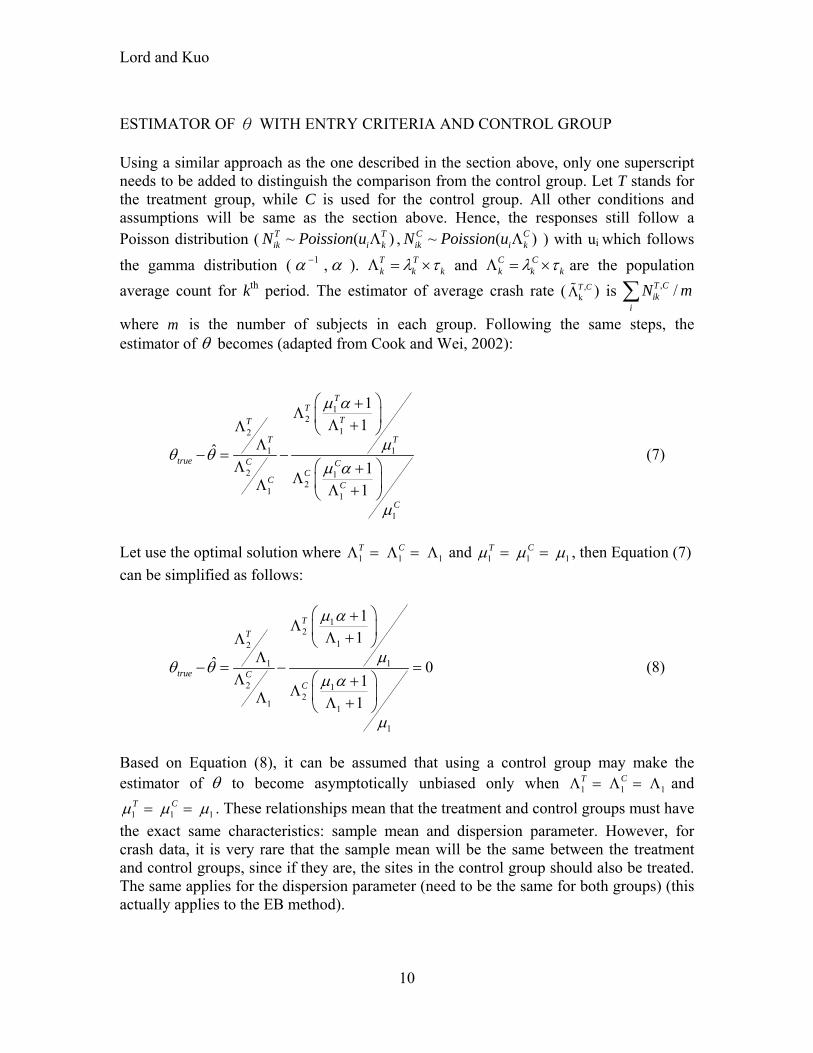
ESTIMATOR OF θ WITH ENTRY CRITERIA AND CONTROL GROUP Using a similar approach as the one described in the section above, only one superscript needs to be added to distinguish the comparison from the control group. Let T stands for the treatment group, while C is used for the control group. All other conditions and assumptions will be same as the section above. Hence, the responses still follow a Poisson distribution ( ~ ( )T T
ik i kN Poission u , ~ ( )C Cik i kN Poission u ) with ui which follows
the gamma distribution ( 1 , ). T Tk k k
and C C
k k k are the population
average count for kth period. The estimator of average crash rate ( ,kT C ) is , /T C
iki
N m
where m is the number of subjects in each group. Following the same steps, the estimator of becomes (adapted from Cook and Wei, 2002):
12
12
1 1
2 12
11
1
1
1
ˆ1
1
TT
TT
T T
true C CC
CC
C
(7)
Let use the optimal solution where 1 1 1 T C and 1 1 1 T C , then Equation (7)
can be simplified as follows:
12
12
1 1
2 12
11
1
1
1
ˆ 01
1
T
T
true CC
(8)
Based on Equation (8), it can be assumed that using a control group may make the estimator of to become asymptotically unbiased only when 1 1 1 T C and
1 1 1 T C . These relationships mean that the treatment and control groups must have
the exact same characteristics: sample mean and dispersion parameter. However, for crash data, it is very rare that the sample mean will be the same between the treatment and control groups, since if they are, the sites in the control group should also be treated. The same applies for the dispersion parameter (need to be the same for both groups) (this actually applies to the EB method).
Lord and Kuo
11
BOUNDARY CONDITIONS FOR As discussed above, the RTM and site selection effects create two different biases. Similar to continuous data, the RTM does not exist when the correlation ( ) between
1N and 2N is equal to one. In this case, either 1 1 or . When this happens,
all the bias associated with estimating disappears However, in practice, observing perfect correlation where the RTM is equal to zero rarely exists or ever happens. The site selection bias on will become zero when 1 1 , as shown in Equation (6).
In other words, site selection bias will always exist until C<0, even when 0 (the
responses in the before and after period are independent or 0 ). This result is consistent with Davis’ (2000) findings (see Eq. 16 in his paper), but only when the selection effect or entry criterion is equal to C<0. Thus, when C is a nonnegative integer (0, 1, 2, …), the site selection bias will constantly be present. This also means that for crash data, this bias of will exist even when sites with a minimum of 1 crash (as long as ) are included. It should be pointed out that for count data, the site selection effect will cause different biases for different estimators: 1 2, , , and , as pointed out
earlier. Some of these will be discussed in subsequent publications or can also be found in Kuo (2012). METHODOLOGY AND SIMULATION PROTOCOL This section describes the methodology and simulation protocol used for estimating the bias for the following scenarios. Appendix B presents a glossary of the terms used in this paper. SCENARIO ANALYSIS Five scenarios were used to examine possible factors related to site-selection bias. Scenario 1 compared the four most common types of before-after studies: the Naïve method, using a control group (CG), the EB method based on the method of moment (EBMM), and the EB method based on a control group (EBCG). Then, these were compared with the new proposed method to adjust the naïve estimator. Scenario 2 examined different values for the dispersion parameter: from 0.25 (small heterogeneity) to 7.0 (very large heterogeneity). Scenario 3 studied the effects of sample size on the bias: 10 (small), 30 (medium), and 100 (large). More specifically, this scenario assesses whether the estimator, based on Equation (6), is influenced when the sample size does not tend towards infinity. Scenario 4 analyzed the magnitude associated with the safety effectiveness for three values: 0.90 (high), 0.70 (medium), and 0.50 (low). Finally, Scenario 5 looked at the effects related to the standard deviation of the index of safety effectiveness on the bias: 0.05 (small), 0.10 (medium), and 0.20 (large). For all scenarios, the entry criteria were assumed to vary from C=0 (i.e., 1 1iN ) to C=5.
The data generation procedure followed a Poisson-gamma distribution to generate the
Lord and Kuo
12
mean response rate and observed number of counts. m (i=1 to m ) observations were selected randomly for the treatment group only when the response was larger than the
entry criteria ( 11
t
ijjN C
). These sites are labeled as 1
TijN and 2
TijN . The sample size
was equal to 100 and the safety effectiveness was equal to 0.50 unless the scenarios required these two variables to change. The safety effectiveness for Scenario 5 was equal to 0.90, in order to avoid having equal to zero. Note that Scenarios 1 and 2 were analyzed simultaneously. The equations for the four methods and the one proposed in this study are as follows:
Naïve method: 2 1 21 1 1 1
1 11 1 1 1
|ˆ
( )
n n Tij ij iji j i j
n n Tij iji j
t
j
t
i
t t
N N C N
N C N
(9)
CG method:1
1
2 21 1
221 1 1
1 1 1 1 11
ˆˆ
ˆˆ
ˆ
n nt T
i iji i
Ccn n n nt t ijTi
i ij Cci i i i iji
j
j j
N
NN
N
(10)
Empirical Bayes method:
21 1
11 1
11 1
2
11 1
ˆ
Var1
n Tiji j
n Tiji j
n Tiji j
n Tiji j
t
t
t
t
N
M
M
M
(11)
Proposed Adjustment method (based on Equation (6) and the estimators from Geyer (2007)):
1 1
1 1
11
1
ˆ ˆ( 1)
ˆ
ˆˆ ˆ(
1( 1)
(1 )( 1
1
)1
1( 1)
(1 )( 1)
)
adjusted naive
naive
CP N CP N C
CP N CP N C
(12)
Lord and Kuo
13
Where, 1 11 1
1ˆn t
Tij
i j
Nn
(13)
22 1 1
2 1
2 1
(( ) )1
( )
( )
i i
i i
i i
E N N C
E N N C
E N N C
(14)
Note: The index for all the methods were not adjusted for the sample size by the approach proposed by Hauer (1997). SIMULATION PROTOCOL The simulated data was generated using the software R (R Development Core Team, 2006). The general steps were as follows:
1) For each dispersion parameter, generate the subject-specific random effect
( iu ), which follows a gamma distribution 1~ ,gamma and generate a
crash count with a Poisson mean ( 1 1~i i i iN Poisson u ) for each site i ,
where i , the sample mean, was equal to 1. Sample mean values equal to 3, 5
and 10 were also tested, but the results are not presented here due to space constraints. All the results were consistent with the values presented in this paper, expect at the boundary when is almost equal to zero (to be discussed in another paper).
2) Generate three years of counts in the before period using 1i for each site.
Generate the data for m = 5,000 sites, but randomly select 100, 30 and 10 sites depending on the scenario.
3) Only for Scenario 5: Generate the treatment effectiveness for each site using a
normal distribution, 2~ ,N , where = 0.90 and 2 = 0.05, 0.10 or
0.20. (note: the index could theoretically show an increase)
4) Estimate the crash mean rate ( 2ˆ
i ) for each site in after period equal to the
product of the above matrixes ( 1ˆ
i ). Then, generate three years of count
using the Poisson distribution, 2 2~i iN Poisson .
5) Then, n sites are selected as the sample whose observed crash numbers are larger than the entry criteria (0,…, 5), and its effectiveness can be estimated using Equations (9), (10), (11), or (12).
6) When the control group is used, θ is equal to 1. In other words, there is no different for mean rate between before and after period.
7) Repeat steps 2 to 6 for a total of 1,000 times, and estimate the various biased estimates 1000
ˆ .
Lord and Kuo
14
SIMULATION RESULTS This section describes the results based on the simulation. They are presented for each scenario separately.
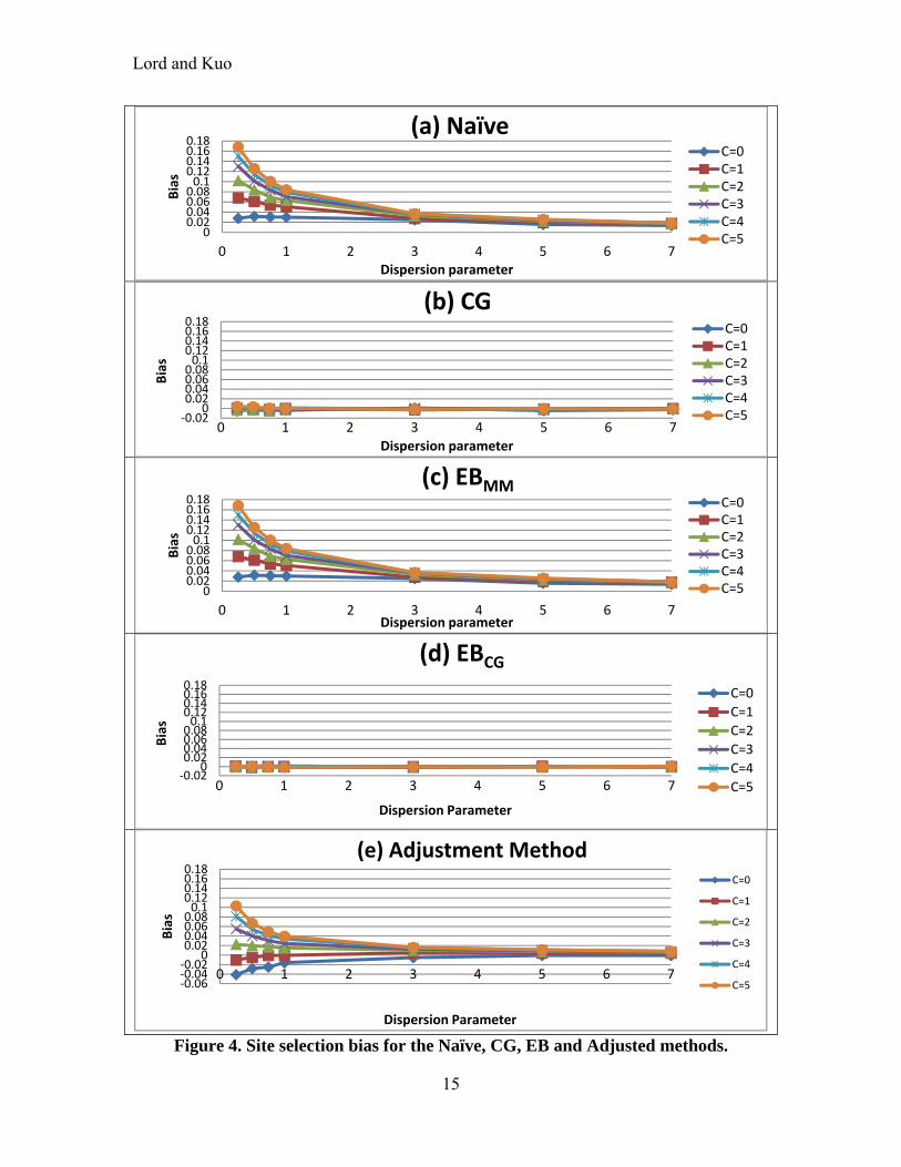
SCENARIO 1 - RESULTS Figure 4 shows the site selection bias for the Naïve, CG, EBMM,EBCG and the Adjusted methods. Overall, this figure shows that the bias goes down as the dispersion parameter increases, except when is almost equal to zero (at least for C < 3) (recall that if 0C ,
1 1iN , etc.). This was expected given the characteristics of Equation (6). The greater the
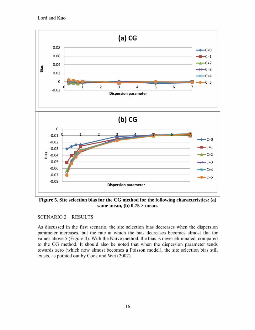
entry criteria, more biased the estimate will be. Among the four methods, the Naïve (Figure 4a) and the EBMM (Figure 4c) methods are the ones that are the most affected by the site selection bias; can be over-estimated by as much as 36%. As discussed by Cook and Wei (2002), unless the RTM is completely non-existent (), will be biased if an entry criteria is used (e.g., the bias never equals zero when 7 ). Readers may be surprised to see that the EBMM method does not reduce or eliminate the RTM when site selection effects are included. This is caused by the fact that the MM estimate is calculated using the characteristics of the truncated sample rather than the full population or non-truncated sample. Appendix A describes in greater details the conditions when the EB method (both for EBMM and EBCG) can be biased. When a control group is used, the bias can be theoretically eliminated. For the CG method (Figure 4b), the control group needs to have the same characteristics, i.e., the same sample mean and variance (which can be used for obtaining the dispersion parameter) as the truncated sample used for the Naïve method (see right-hand side of Figure 3). As explained above, it may be difficult to find datasets with the exact same characteristics as for the treatment group in practice. For the EBCG method (Figure 4d), the control group needs to have the same characteristics as the full sample (or sample population) from which the truncated data were used for calculating the Naïve or EBMM estimates (see left-hand side of Figure 3). Again, the reader is referred to Appendix A for the conditions when the EBCG can be biased. The application of the control group is further explored in Figure 5. Figure 5a is the same as Figure 4b, and is used to compare the results with the other figure below. Figure 5b shows that when the control group does not have the same characteristics, in this case the same sample mean, the site selection bias is still present, although it is still smaller than using the Naïve before-after method. Furthermore, the bias is also in the opposite direction (under-estimate ). It should be noted that the estimator based on Equation (6) can estimate the site-selection bias accurately when the true value of the mean and variance are known. Even when a control group is not available, the simulation results show that the estimator can still reduce the bias by approximately 50% simply by utilizing the truncated sample mean and variance, as shown in Figure 4e and Equation (12). This characteristic has been validated using observed data, as documented in Kuo (2012).
Lord and Kuo
15
Figure 4. Site selection bias for the Naïve, CG, EB and Adjusted methods.
00.020.040.060.080.10.120.140.160.18
0 1 2 3 4 5 6 7
Bias
Dispersion parameter
(a) NaïveC=0C=1C=2C=3C=4C=5
‐0.020
0.020.040.060.080.10.120.140.160.18
0 1 2 3 4 5 6 7
Bias
Dispersion parameter
(b) CGC=0C=1C=2C=3C=4C=5
00.020.040.060.080.10.120.140.160.18
0 1 2 3 4 5 6 7
Bias
Dispersion parameter
(c) EBMMC=0C=1C=2C=3C=4C=5
‐0.020
0.020.040.060.080.10.120.140.160.18
0 1 2 3 4 5 6 7
Bias
Dispersion Parameter
(d) EBCG
C=0
C=1
C=2
C=3
C=4
C=5
‐0.06‐0.04‐0.02
00.020.040.060.080.10.120.140.160.18
0 1 2 3 4 5 6 7
Bias
Dispersion Parameter
(e) Adjustment MethodC=0
C=1
C=2
C=3
C=4
C=5
Lord and Kuo
16
Figure 5. Site selection bias for the CG method for the following characteristics: (a) same mean, (b) 0.75 × mean.
SCENARIO 2 − RESULTS
As discussed in the first scenario, the site selection bias decreases when the dispersion parameter increases, but the rate at which the bias decreases becomes almost flat for values above 5 (Figure 4). With the Naïve method, the bias is never eliminated, compared to the CG method. It should also be noted that when the dispersion parameter tends towards zero (which now almost becomes a Poisson model), the site selection bias still exists, as pointed out by Cook and Wei (2002).
‐0.02
0
0.02
0.04
0.06
0.08
0 1 2 3 4 5 6 7
Bias
Dispersion parameter
(a) CG
C=0
C=1
C=2
C=3
C=4
C=5
‐0.08
‐0.07
‐0.06
‐0.05
‐0.04
‐0.03
‐0.02
‐0.01
0
0 1 2 3 4 5 6 7
Bias
Dispersion parameter
(b) CG
C=0
C=1
C=2
C=3
C=4
C=5

Lord and Kuo
17
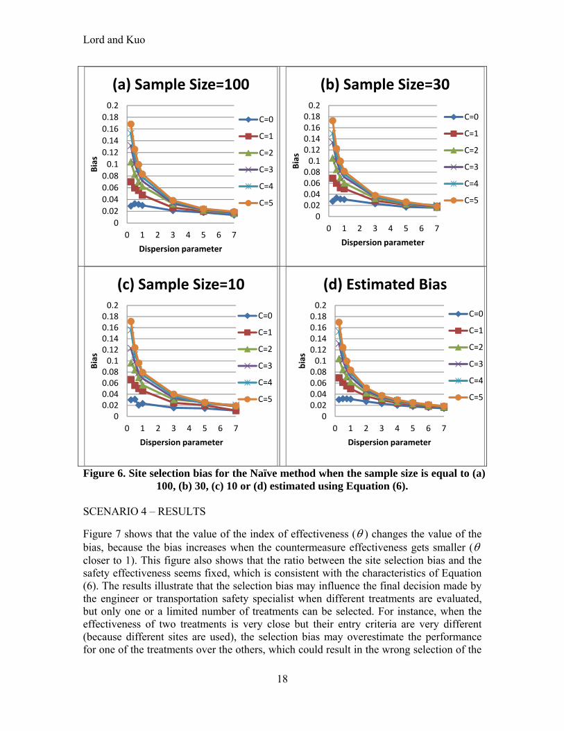
SCENARIO 3 – RESULTS
Figure 6 shows that the sample size related to the treatment group does not affect the bias considerably. When the sample size is over 30, the bias obtained by using the Naïve method, Equation (9), and the one estimated with Equation (6) are very close. Furthermore, there is a slight difference between the simulated bias and the estimated one when the dispersion parameter is less than 1 (most often observed in crash data). However, the maximum difference (sample size=10, C=0) is about 0.04 when the safety effectiveness is equal to 0.50. Hence, Equation (6) which was derived by assuming that the sample size is close to infinity (∞) may be used for estimating site selection biases even the sample size is small.
Lord and Kuo
18
Figure 6. Site selection bias for the Naïve method when the sample size is equal to (a) 100, (b) 30, (c) 10 or (d) estimated using Equation (6).
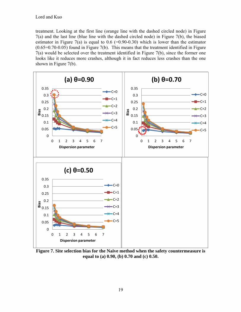
SCENARIO 4 – RESULTS
Figure 7 shows that the value of the index of effectiveness ( ) changes the value of the bias, because the bias increases when the countermeasure effectiveness gets smaller (closer to 1). This figure also shows that the ratio between the site selection bias and the safety effectiveness seems fixed, which is consistent with the characteristics of Equation (6). The results illustrate that the selection bias may influence the final decision made by the engineer or transportation safety specialist when different treatments are evaluated, but only one or a limited number of treatments can be selected. For instance, when the effectiveness of two treatments is very close but their entry criteria are very different (because different sites are used), the selection bias may overestimate the performance for one of the treatments over the others, which could result in the wrong selection of the
0
0.02
0.04
0.06
0.08
0.1
0.12
0.14
0.16
0.18
0.2
0 1 2 3 4 5 6 7
Bias
Dispersion parameter
(a) Sample Size=100
C=0
C=1
C=2
C=3
C=4
C=5
00.020.040.060.080.1
0.120.140.160.180.2
0 1 2 3 4 5 6 7
Bias
Dispersion parameter
(b) Sample Size=30
C=0
C=1
C=2
C=3
C=4
C=5
00.020.040.060.080.1
0.120.140.160.180.2
0 1 2 3 4 5 6 7
Bias
Dispersion parameter
(c) Sample Size=10
C=0
C=1
C=2
C=3
C=4
C=5
00.020.040.060.080.1
0.120.140.160.180.2
0 1 2 3 4 5 6 7
bias
Dispersion parameter
(d) Estimated Bias
C=0
C=1
C=2
C=3
C=4
C=5
Lord and Kuo
19
treatment. Looking at the first line (orange line with the dashed circled node) in Figure 7(a) and the last line (blue line with the dashed circled node) in Figure 7(b), the biased estimator in Figure 7(a) is equal to 0.6 (=0.90-0.30) which is lower than the estimator (0.65=0.70-0.05) found in Figure 7(b). This means that the treatment identified in Figure 7(a) would be selected over the treatment identified in Figure 7(b), since the former one looks like it reduces more crashes, although it in fact reduces less crashes than the one shown in Figure 7(b).
Figure 7. Site selection bias for the Naïve method when the safety countermeasure is equal to (a) 0.90, (b) 0.70 and (c) 0.50.
0
0.05
0.1
0.15
0.2
0.25
0.3
0.35
0 1 2 3 4 5 6 7
Bias
Dispersion parameter
(a) θ=0.90
C=0
C=1
C=2
C=3
C=4
C=5
0
0.05
0.1
0.15
0.2
0.25
0.3
0.35
0 1 2 3 4 5 6 7
Bias
Dispersion parameter
(b) θ=0.70
C=0
C=1
C=2
C=3
C=4
C=5
0
0.05
0.1
0.15
0.2
0.25
0.3
0.35
0 1 2 3 4 5 6 7
Bias
Dispersion parameter
(c) θ=0.50
C=0
C=1
C=2
C=3
C=4
C=5
Lord and Kuo
20
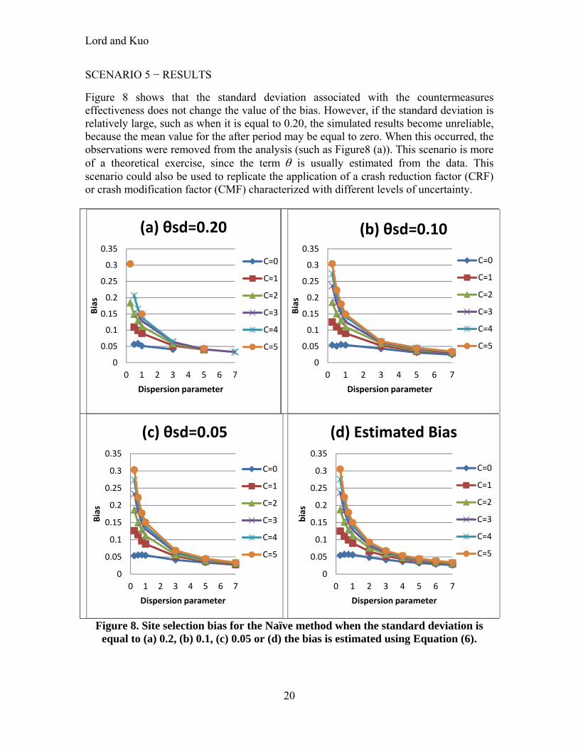
SCENARIO 5 − RESULTS
Figure 8 shows that the standard deviation associated with the countermeasures effectiveness does not change the value of the bias. However, if the standard deviation is relatively large, such as when it is equal to 0.20, the simulated results become unreliable, because the mean value for the after period may be equal to zero. When this occurred, the observations were removed from the analysis (such as Figure8 (a)). This scenario is more of a theoretical exercise, since the term is usually estimated from the data. This scenario could also be used to replicate the application of a crash reduction factor (CRF) or crash modification factor (CMF) characterized with different levels of uncertainty.
Figure 8. Site selection bias for the Naïve method when the standard deviation is equal to (a) 0.2, (b) 0.1, (c) 0.05 or (d) the bias is estimated using Equation (6).
0
0.05
0.1
0.15
0.2
0.25
0.3
0.35
0 1 2 3 4 5 6 7
Bias
Dispersion parameter
(a) θsd=0.20
C=0
C=1
C=2
C=3
C=4
C=5
0
0.05
0.1
0.15
0.2
0.25
0.3
0.35
0 1 2 3 4 5 6 7
Bias
Dispersion parameter
(b) θsd=0.10
C=0
C=1
C=2
C=3
C=4
C=5
0
0.05
0.1
0.15
0.2
0.25
0.3
0.35
0 1 2 3 4 5 6 7
Bias
Dispersion parameter
(c) θsd=0.05
C=0
C=1
C=2
C=3
C=4
C=5
0
0.05
0.1
0.15
0.2
0.25
0.3
0.35
0 1 2 3 4 5 6 7
bias
Dispersion parameter
(d) Estimated Bias
C=0
C=1
C=2
C=3
C=4
C=5
Lord and Kuo
21
SUMMARY AND CONCLUSIONS This study has examined how setting an entry criterion influences the estimation of traffic safety countermeasures. The goal consisted in estimating how the bias changes for four commonly types of before-after studies: the Naïve, the CG and the EBMM and EBCG methods. Those methods were then compared to a new proposed method that could be used to adjust the naïve estimator when a control group is not available. Five scenarios were evaluated: a direct comparison of the methods, different sample sizes, different dispersion parameter values, different safety effectiveness values, and different standard deviation values associated with the safety effectiveness. The analysis was carried out using simulated data, but theoretical derivations were also presented in Appendix A to support results documented in this study. The study results showed that among all methods evaluated, the Naïve and the EBMM methods are the ones that are the most significantly affected by the selection bias. Using a control group (CG) or the EBCG can eliminate the site selection bias, as long as the characteristics of the control group are exactly the same as for the treatment group. For the CG method, the characteristics of the CG need to be the same as the characteristics of the truncated sample (see right-hand side of Figure 3). For the EBCG, the characteristics of the control group need to be the same as the full or non-truncated sample (see left-hand side of Figure 3). In practice, this may not be possible. However, using the approach proposed in this study to adjust, but not eliminate, the naïve estimator can partially eliminate site-selection bias, even when biased estimators of the mean and dispersion parameter of a truncated Negative Binomial distribution are used. To do this, the researcher or safety analyst simply needs to compute the naïve estimator, calculate the sample mean and the variance of the data in order to get the dispersion parameter, and incorporate the values into Equation (6) to get an estimate of the bias. Then, once the bias is estimated, the index can be adjusted using Equation (12). Based on the simulated scenarios (also supported theoretically), the study results also showed that higher entry criteria, larger values of the index ( ), and smaller dispersion parameter values will cause a higher site selection biased estimate. It should be pointed out that the assumptions made in this study did not influence the validity of the analysis. In fact, the analyses presented in this paper have been validated using observed data, as documented in Kuo (2012). Given the nature of the work documented in this paper, there are several avenues for further work. First, since the estimator of the site-selection bias, Equation (6), only estimates about 50% of the bias when a control group is not available, it may be beneficial to apply more advanced techniques to estimate the parameters of a truncated Negative Binomial model (or truncated Normal distribution for continuous data) in order to obtain more precise estimates. Second, the site selection effect may be influenced by missing data. The estimator of the selection bias may not be affected when the missing data are randomly distributed since the samples are still representative of the population. On the other hand, if the missing data are systematic, such as those associated with property damage only or possible injury (classified as injury C) crashes or for certain categories of collision types, the estimator may become more biased. Hence, further work
Lord and Kuo
22
needs to be conducted on this topic. Third, guidelines should be developed to define what the entry criterion should be used when it is not known (e.g., minimum value in sample, MUTCD, etc.). Fourth, one should examine site selection effects close to the boundary when 0 as a function of different mean values for the before period. Fourth, statistical tests or methodologies should be developed to ensure that the data collected for the control group when the EB method is used is the same as the full data from which the truncated distribution is used (which may not be possible to find out). Although the EBCG method has been (and still is) frequently used among transportation safety analysts, very few ever compare the characteristics of the treatment and control groups. Researchers automatically assume that the NB regression models estimated from the control group has the same characteristics as the sites selected for potential treatment. Finally, a simpler approach for displaying the site selection bias should be done. Tables based on the sample mean ( 1 ), entry criteria, and the level of dispersion could be
provided in the Highway Safety Manual (2010) or any similar types of documents. ACKNOWLEDGEMENTS The authors would like to thank Dr. Gary A. Davis from the University of Minnesota and Dr. Ezra Hauer, Professor Emeritus at the University of Toronto, for their input. The authors also thank Dr. Jeff Hart from Texas A&M University for his review and suggestions related to Appendix A. REFERENCES Abbess, C., Jarrett, D, Wright, C., 1981. Accidents at blackspots: Estimating the effectiveness of remedial treatment, with special reference to the “regression-to-mean” effect, Traffic Engineering and Control 22, 535-542. American Association of State Highway and Transportation Officials, 2010. Highway Safety Manual 1st Edition, Washington, DC. Chuang-Stein, C., Tong, D., 1997. The impact and implication of regression to the mean on the design and analysis of medical investigations. Statistical Methods in Medical Research 6, 115-128. Cook, R., Wei, W., 2002. Selection effects in randomized trials with count data, Statistics in Medicine 21, 515-531. Copas, J., 1997. Using regression models for prediction: shrinkage and regression to the mean. Statistical Methods in Medical Research 6, 167-183. Danielsson, S., 1986. A comparison of two methods for estimating the effect of a countermeasure in the presence of regression effects. Accident Analysis and Prevention 18,13–23.
Lord and Kuo
23
Davis, C.E., 1976. The effect of regression to the mean in epidemiologic and clinical studies. American Journal of Epidemiology ,Vol.104, pp493–98. Davis, G., 2000. Accident reduction factors and causal inference in traffic safety studies: a review. Accident Analysis & Prevention, 32, 95–109. FHWA, 2010. Manual on Uniform Traffic Control Devices. Federal Highway Administration, Washington, D.C. Geyer, C.J., 2007. Lower-Truncated Poisson and Negative Binomial Distributions. Working paper written for the software r. University of Minnesota, MN. (available: http://cran.r-project.org/web/packages/aster/vignettes/trunc.pdf) Hamed M.M., Al-Eideh B.M., Al-Sharif M.M. 1999. Traffic accidents under the effect of the Gulf crisis, Safety Science, 33, 59-68 Hauer, E., 1980a. Bias-by-Selection: Overestimation of the Effectiveness of Safety Countermeasures Caused by the Process of Selection for Treatment, Accident Analysis & Prevention, 12, 113-117 Hauer, E., 1980b. Selection for treatment as a source of bias in before-and-after studies. Traffic Engineering and Control 21, 419–421. Hauer, E., 1997. Observational Before-After Studies in Road Safety. Pergamon Publications, London. Hauer, E., Byer, P., Joksch, H., 1983. Bias-by-selection: The Accuracy of an unbiased estimator. Accident Analysis & Prevention 15, 323-328. Hauer, E. Persaud, B., 1983. Common bias in before-and-after accident comparisons and its elimination. Transportation Research Record 905, 164-174. Hauer, E., Persaud, B., 1984. Problem of Identifying Hazardous Locations Using Accident Data. Transportation Research Record 975, 36-43. Kuo, P.-F., 2012. Examining the Effects of Site Selection Criteria for Evaluating the Effectiveness of Traffic Safety Countermeasures. Ph.D. Dissertation. Zachry Department of Civil Engineering, Texas A&M University, College Station, TX. Kuo, P.-F., Lord, D., 2012. Accounting for Site-Selection Bias in Before-After Studies for Continuous Distributions: Characteristics and Application Using Speed Data. Paper presented at the 91st Annual Meeting of the Transportation Research Board, Washington, D.C. Lawless J., Fong D., 1999. State duration models in clinical and observational studies. Statistics in Medicine 18, 2365-2376
Lord and Kuo
24
Li W., Carriquiry, A., Pawlovich, M., Welch, T. , 2008. The Choice of Statistical Models in Road Safety Countermeasure Effectiveness Studies in Iowa. Accident Analysis and Prevention 40, 1531-1542. Lord, D., and F. Mannering, 2010. The Statistical Analysis of Crash-Frequency Data: A Review and Assessment of Methodological Alternatives. Transportation Research - Part A, Vol. 44, No. 5, pp. 291-305. Maher, M., Mountain, L., 2009. The sensitivity of estimates of regression to the mean. Accident Analysis & Prevention 4, 861-868. Miaou, S.-P., J. J. Song, and B. K. Mallick. 2003. Roadway Traffic-Crash Mapping: A Space-Time Modeling Approach. Journal of Transportation and Statistics 4, Miranda-Moreno, L., Fu, L., Ukkusuri, S., Lord, D., 2009. How to Incorporate Accident Severity and Vehicle Occupancy into the Hotspot Identification Process? Transportation Research Record 2102, 53-60. Noland, R., 2003. Traffic fatalities and injuries: the effect of changes in infrastructure and other trends. Accident Analysis and Prevention 35, 599-611. Park, E., Park, J., Lomax, T., 2010. A fully Bayesian multivariate approach to before–after safety evaluation. Accident Analysis & Prevention 42, 1118-1127. Park, P., and D. Lord., 2010. Investigating Regression-to-the-Mean in Before-and-After Speed Data. Transportation Research Record 2165, 52-58. Pearl, J., 2009. Causality: Models, Reasoning, and Inference. 2nd edition Cambridge University Press, New York. Persaud, B., 2001. Statistical Methods in Highway Safety Analysis, NCHRP Synthesis of Highway Practice 295, Transportation Research Board, National Research Council, Washington, DC. Persaud B., Lyon, C., 2007. Empirical Bayes before–after studies: lessons learned from two decades of experience and future directions, Accident Analysis and Prevention 39, 546–555. R Development Core Team, 2006. R: A Language and Environment for Statistical Computing. R Foundation for Statistical Computing. Vienna, Austria, ISBN 3-900051-07-0. Rock, S. M., 1995. Impact of the 65 mph speed limit on accidents, deaths, and Injuries in Illinois. Accident Analysis and Prevention, 27, 207-214.
Lord and Kuo
25
Robbins, H., 1956. An Empirical Bayes Approach to Statistics. Proceedings of the Third Berkeley Symposium on Mathematical Statistics and Probability, Volume 1: Contributions to the Theory of Statistics, 157–163. Rubin, D., 1977. Assignment of treatment group on the basis of a covariate. Journal of Educational and Behavioral Statistics 2, 1-26. Samuels, M.L., 1991. Statistical Reversion Toward the Mean: More Universal than Regression Toward the Mean. The American Statistician 45 (4), 344–346. Stingler, S., 1997. Regression towards the mean, historically considered. Statistical Methods in Medical Research 6, 103-114. Tarko, A., Eranky, S., Sinha, K., 1998. Methodological considerations in the development and use of crash reduction factors. Preprint CD. 77th Annual Meeting of the Transportation Research Board, Washington, DC. Wright, C., Abbess, C., Jarrett, D., 1988. Estimating the regression-to-mean effect associated with road accident black spot treatment: Towards a more realistic approach. Accident Analysis & Prevention, 20, 199-214.
Lord and Kuo
26
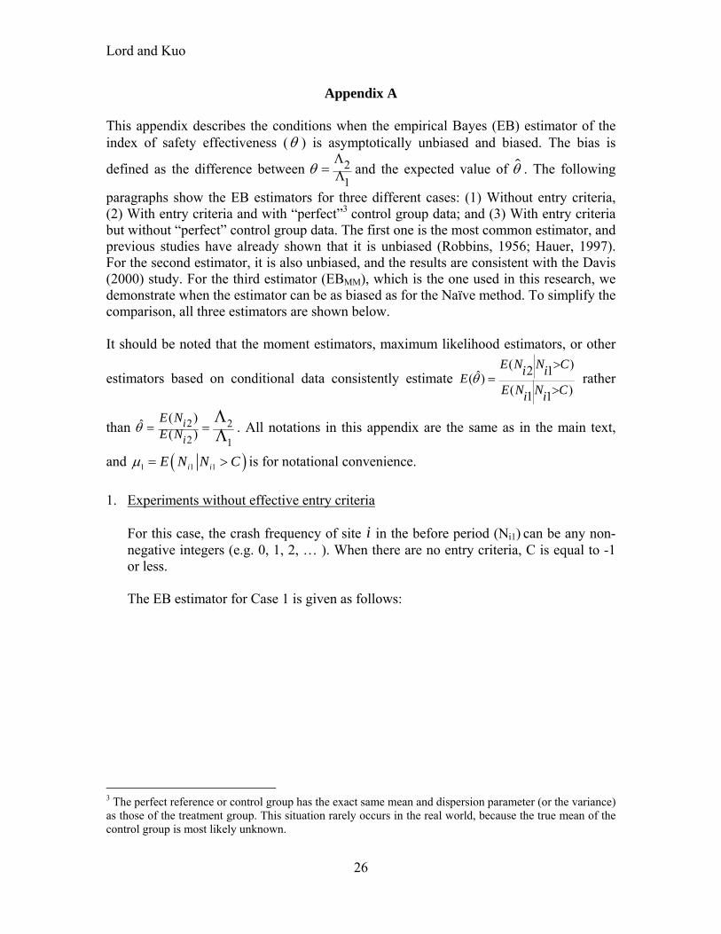
Appendix A This appendix describes the conditions when the empirical Bayes (EB) estimator of the index of safety effectiveness ( ) is asymptotically unbiased and biased. The bias is
defined as the difference between 2
1
and the expected value of . The following
paragraphs show the EB estimators for three different cases: (1) Without entry criteria, (2) With entry criteria and with “perfect”3 control group data; and (3) With entry criteria but without “perfect” control group data. The first one is the most common estimator, and previous studies have already shown that it is unbiased (Robbins, 1956; Hauer, 1997). For the second estimator, it is also unbiased, and the results are consistent with the Davis (2000) study. For the third estimator (EBMM), which is the one used in this research, we demonstrate when the estimator can be as biased as for the Naïve method. To simplify the comparison, all three estimators are shown below. It should be noted that the moment estimators, maximum likelihood estimators, or other
estimators based on conditional data consistently estimate ( )2 1ˆ( )( )1 1
E N N Ci iE
E N N Ci i
rather
than 2 2
2 1
( )ˆ( )
i
i
E NE N
. All notations in this appendix are the same as in the main text,
and 1 1 1i iE N N C is for notational convenience.
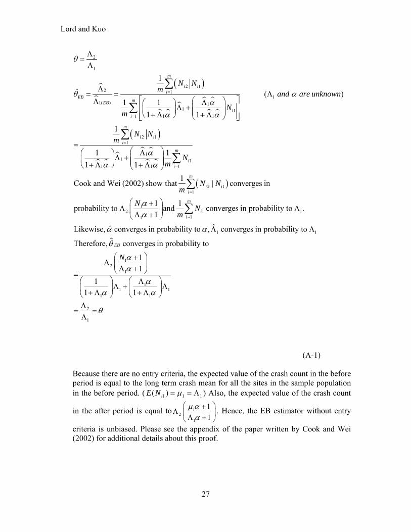
1. Experiments without effective entry criteria
For this case, the crash frequency of site i in the before period (Ni1) can be any non-negative integers (e.g. 0, 1, 2, … ). When there are no entry criteria, C is equal to -1 or less. The EB estimator for Case 1 is given as follows:
3 The perfect reference or control group has the exact same mean and dispersion parameter (or the variance) as those of the treatment group. This situation rarely occurs in the real world, because the true mean of the control group is most likely unknown.
Lord and Kuo
27
2
1
2 12 1
11( ) 1
1 11 11
2 11
11 1
1 1 1
2 1
1
ˆ ( )1 1
1 1
1
1 1
1 1
1Cook and Wei (2002) show that | converges in
m
i ii
EBmEB
ii
m
i ii
m
ii
i i
N Nm
and are unknown
Nm
N Nm
Nm
N Nm
1
12 1 1
11
1 1
12
1
1 1probability to and converges in probability to .
1
ˆˆLikewise, converges in probability to , converges in probability to
Therefore, converges in probability to
1
1
m
i
m
ii
EB
NN
m
N
11 1
1 1
2
1
11 1
(A-1)
Because there are no entry criteria, the expected value of the crash count in the before period is equal to the long term crash mean for all the sites in the sample population in the before period. ( 111)( iNE ) Also, the expected value of the crash count
in the after period is equal to 12
1
1
1
. Hence, the EB estimator without entry
criteria is unbiased. Please see the appendix of the paper written by Cook and Wei (2002) for additional details about this proof.
Lord and Kuo
28
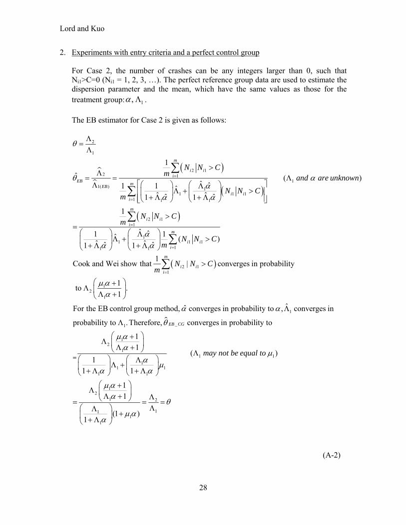
2. Experiments with entry criteria and a perfect control group For Case 2, the number of crashes can be any integers larger than 0, such that Ni1>C=0 (Ni1 = 1, 2, 3, …). The perfect reference group data are used to estimate the dispersion parameter and the mean, which have the same values as those for the treatment group: 1, .
The EB estimator for Case 2 is given as follows:
2
1
2 12 1
11( ) 1
1 1 11 1 1
2 11
11 1 1
11 1
1
ˆ ( )ˆ ˆ1 1 ˆ
ˆ ˆˆ ˆ1 1
1
ˆ ˆ1 1ˆ ( )ˆ ˆˆ ˆ1 1
Cook and Wei show that
m
i ii
EBm
EB
i ii
m
i ii
m
i ii
N N Cm
and are unknown
N N Cm
N N Cm
N N Cm
2 11
12
1
1
_1
12
1
1| converges in probability
1to .
1
ˆˆFor the EB control group method, converges in probability to , converges in
probability to . Therefore, converges in probability to
1
1
m
i ii
EB CG
N N Cm
1 1
11 1
1 1
12
1 2
111
1
( )1
1 1
1
1
(1 )1
may not be equal to
(A-2)
Lord and Kuo
29
The long-term mean and dispersion parameter values are estimated using a control group or regression model based on the control group. As in the first case, the EB estimator is unbiased. However, in practice, the characteristics of the control group may not be the same as the one used for the treatment group.
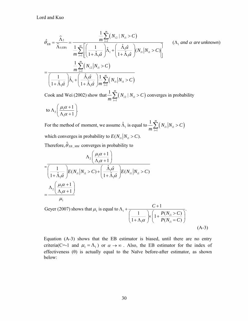
3. Experiments with entry criteria and without perfect control group data. For this case, the number of crashes can be any integers larger than 0, such that Ni1>C=0 (Ni1 = 1, 2, 3, …). The reference group data are used to estimate the dispersion parameter and the mean, which have different values than those from the treatment group. The EB estimator for Case 3, based on the method of moment, is given as follows:
Lord and Kuo
30
2 12 1
11( ) 1
1 1 11 1 1
2 11
11 1 1
11 1
1|
ˆ ( )ˆ ˆ1 1 ˆ ( )
ˆ ˆˆ ˆ1 1
1
ˆ ˆ1 1ˆˆ ˆˆ ˆ1 1
Cook and Wei (2002) show that
m
i ii
EBm
EB
i ii
m
i ii
m
i ii
N N Cm
and are unknown
N N Cm
N N Cm
N N Cm
2 11
12
1
1 1 11
1 1
_
1| converges in probability
1to .
1
1ˆFor the method of moment, we assume is equal to
which converges in probability to ( ).
Therefore, converges in probability t
m
i ii
m
i ii
i i
EB MM
N N Cm
N N Cm
E N N C
12
1
11 1 1 1
1 1
12
1
1
1 1
1
1 1
o
11ˆ ˆ1
( ) ( )ˆ ˆˆ ˆ1 1
11
1Geyer (2007) shows that is equal to .
( )11
1 ( )
i i i i
i
i
E N N C E N N C
C
P N C
P N C
(A-3)
Equation (A-3) shows that the EB estimator is biased, until there are no entry criteria(C=-1 and 11 ) or . Also, the EB estimator for the index of effectiveness (θ) is actually equal to the Naïve before-after estimator, as shown below:

Lord and Kuo
31
2 11
_
11 1 1
1 1 1
2 11
1 11 1
1 111 1
2 11
1 11
|ˆ
ˆ ˆ1 ˆˆ ˆˆ ˆ1 1
ˆ ˆˆ ˆˆ ˆ1 1
m
i ii
EB MMm
i ii
m
i ii
m
i i mi
i ii
m
i iim
i ii
N N C
N N C
N N C
N N Cm
N N Cm
N N C
N N C
(A-4)
In sum, using a biased estimate of 1 is the main reason why the EBmm estimator of is also biased.
Appendix B The glossary of the terms used in the paper is as follows:
: the safety effectiveness, 0 1 (can be theoretically higher, but not in this study); C : the entry criterion; n : the sample size; : the dispersion parameter (of the NB model);
1ijN : the observed response for site i in j year (in the before period) for count data;
2ijN : the observed response for site i in j year (in the after period) for count data;
1 1,T Ci i : the mean response rate for site i (T: treatment group, C: control group)
in the before period;
2 2,T Ci i : the mean response rate for site i (T: treatment group, C: control group)
in the after period;
1 1,T Cij ijN N : the observed response for site i (T: treatment group, C: control group) in
j year (in the before period) for count data, 1TijN > C;
2 2,T Cij ijN N : the observed response for site i (T: treatment group, C: control group) in
j year (in the after period) for count data;
W : the weight for sites for the EB method, 1
1
1W
;

Lord and Kuo
32
1 : the estimator for the average crash rate of all sites in the before period;
11 1 1( )i iE N N C for the EBMM method, and 11 for the EBCG method.
: the estimator of dispersion parameter;
21 1 1
1 1
1 1
(( ) )1
( )
( )
i i
i i
i i
E N N C
E N N C
E N N C
for the EBMM method, and for the EBCG
method; and,
1iM : the expected responses for site i for the EB method,
t
1i1 ij1j 1
M W ( ) (1 W) ( )N
.
.