ORIGINAL RESEARCH Open Access

Examining post-fire vegetation recoverywith Landsat time series analysis in threewestern North American forest typesBenjamin C. Bright1* , Andrew T. Hudak1, Robert E. Kennedy2, Justin D. Braaten2 and Azad Henareh Khalyani3

Abstract

Background: Few studies have examined post-fire vegetation recovery in temperate forest ecosystems withLandsat time series analysis. We analyzed time series of Normalized Burn Ratio (NBR) derived from LandTrendrspectral-temporal segmentation fitting to examine post-fire NBR recovery for several wildfires that occurred in threedifferent coniferous forest types in western North America during the years 2000 to 2007. We summarized NBRrecovery trends, and investigated the influence of burn severity, post-fire climate, and topography on post-firevegetation recovery via random forest (RF) analysis.

Results: NBR recovery across forest types averaged 30 to 44% five years post fire, 47 to 72% ten years post fire, and54 to 77% 13 years post fire, and varied by time since fire, severity, and forest type. Recovery rates were generallygreatest for several years following fire. Recovery in terms of percent NBR was often greater for higher-severitypatches. Recovery rates varied between forest types, with conifer−oak−chaparral showing the greatest NBR recoveryrates, mixed conifer showing intermediate rates, and ponderosa pine showing slowest rates. Between 1 and 28% ofpatches had recovered to pre-fire NBR levels 9 to 16 years after fire, with greater percentages of low-severity patchesshowing full NBR recovery.Precipitation decreased and temperatures generally remained the same or increased post fire. Pre-fire NBRand burn severity were important predictors of NBR recovery for all forest types, and explained 2 to 6% ofthe variation in post-fire NBR recovery. Post-fire climate anomalies were also important predictors of NBRrecovery and explained an additional 30 to 41% of the variation in post-fire NBR recovery.

Conclusions: Landsat time series analysis was a useful means of describing and analyzing post-fire vegetationrecovery across mixed-severity wildfire extents. We demonstrated that a relationship exists between post-firevegetation recovery and climate in temperate ecosystems of western North America. Our methods could beapplied to other burned landscapes for which spatially explicit measurements of post-fire vegetation recoveryare needed.

Keywords: burn severity, climate, fire, forest, landsat, North America, satellite imagery, time series, vegetationrecovery

* Correspondence: benjamincbright@fs.fed.us1USDA Forest Service, Rocky Mountain Research Station, 1221 S. Main Street,Moscow, Idaho 83843, USAFull list of author information is available at the end of the article

Fire Ecology

© The Author(s). 2019 Open Access This article is distributed under the terms of the Creative Commons Attribution 4.0International License (http://creativecommons.org/licenses/by/4.0/), which permits unrestricted use, distribution, andreproduction in any medium, provided you give appropriate credit to the original author(s) and the source, provide a link tothe Creative Commons license, and indicate if changes were made.

Bright et al. Fire Ecology (2019) 15:8 https://doi.org/10.1186/s42408-018-0021-9

Resumen

Antecedentes: Pocos estudios han examinado la recuperación post-fuego de la vegetación en ecosistemas debosques templados mediante el análisis de series temporales de imágenes Landsat. Analizamos series temporalesde la Relación de Quemas Normalizadas (NBR) derivadas del ajuste de la segmentación espectro-temporal deLandTrendr para examinar la recuperación post-fuego de la NBR para diferentes incendios ocurridos en tres tiposde bosques de coníferas en el oeste de Norte América durante los años 2000 a 2007. Resumimos las tendencias dela NBR e investigamos la influencia de la severidad de los incendios, el clima post-fuego y la topografía en larecuperación post-fuego de la vegetación a través del análisis de bosques al azar (RF).

Resultados: La recuperación de la NBR entre los tipos forestales promedió del 30 al 44 % cinco años post fuego,de 47 a 72% diez años post fuego, y de 54 al 77% 13 años post fuego y variaron por el tiempo desde el incendio,la severidad de cada fuego y el tipo forestal. La tasa de recuperación fue generalmente más grande después demuchos años de ocurrido los incendios. La recuperación en términos de porcentaje la NBR fue frecuentementemayor para los parches quemados con alta severidad. Las tasas de recuperación variaron entre tipos forestales, enlas que el tipo conífera−roble−chaparral mostró las tasas más altas de recuperación de la NBR, siendo intermediaspara el tipo de coníferas mixtas, y las más lentas para el tipo pino ponderosa. Entre el 1 y el 28% de los parches sehabían recuperado a niveles de NBR pre fuego entre 9 y 16 años del post fuego, con los mayores porcentajes deparches de baja severidad mostrando la más alta recuperación de la NBR. Las precipitaciones decrecieron y lastemperaturas permanecieron iguales o aumentaron durante el post fuego. La NBR previa a los incendios y laseveridad del fuego fueron importantes predictores de la recuperación de la NBR para todos los tipos forestales, yexplicaron del 2 al 6% de la variación en la recuperación de la NBR post fuego. Las anomalías climáticas post fuegofueron también importantes predictores de la recuperación de la NBR y explicaron de un 30 a un 41% adicional enla variación de recuperación post fuego de la NBR.

Conclusiones: El análisis de las series temporales de Landsat resultó un método útil para describir y analizar larecuperación de la vegetación post fuego a través de eventos de fuego de diferente severidad. Demostramos queexiste una relación entre la recuperación de la vegetación post fuego y el clima en bosques templados del oestede Norte América. Nuestros métodos pueden ser aplicados a otros paisajes quemados para los cuales seannecesarias mediciones explícitas de la recuperación de la vegetación.

Abbreviations

%RMSE: Percent root mean square error%VE: percent variance explainedCBI: Composite Burn IndexCURV: McNab’s curvatureDIST: Distance to unburndNBR: differenced Normalized Burn RatioELEV: Elevation above sea levelETM+: Landsat Enhanced Thematic Mapper PlusEVI: Enhanced Vegetation IndexGSP: Post-fire anomaly of growing season precipitationLandTrendr Landsat-based detection of Trends in Dis-turbance and RecoveryMAT: Post-fire anomaly of mean annual temperatureMIR: Model Improvement RatioMMAX: Post-fire anomaly of mean maximum temperaturein warmest monthMMIN: Post-fire anomaly of mean minimum temperaturein coldest monthMTBS: Monitoring Trends in Burn SeverityNBR: Normalized Burn Ratio

NDSWIR: Normalized Difference Shortwave InfraredIndexNDVI: Normalized Difference Vegetation IndexOLI: Landsat Operational Land ImagerRF: Random ForestSLOPE: SlopeSR: Simple RatioSRTM: Shuttle Radar Topographic MissionTM: Landsat Thematic MapperTRASP: Transformed aspectVRI: Vegetation Recovery IndexWINP: Post-fire anomaly of winter precipitation

BackgroundWildfires have burned millions of hectares in westernNorth America in recent decades (Littell et al. 2009, Yanget al. 2015, White et al. 2017). Increased wildfire activity isexpected to continue under warmer and drier conditions(Westerling et al. 2006; Abatzoglou 2016), making ecosys-tem resilience and post-fire vegetation recovery of concernto researchers and land managers (Allen and Breshears2015). Burn severity, the degree to which fire has affected

Bright et al. Fire Ecology (2019) 15:8 Page 2 of 14

vegetation and soil (Keeley 2009), can have a large influ-ence on post-fire vegetation recovery (Chappell 1996;Turner and Romme 1999; Crotteau and Varner III 2013;Meng et al. 2015; Liu 2016; Yang et al. 2017; Meng et al.2018). Other factors that can be important to post-firevegetation recovery include vegetation type (Yang et al.2017; Díaz-Delgado et al. 2002; Epting 2005), climate(Chappell 1996; Meng et al. 2015; Liu 2016), topography(Díaz-Delgado et al. 2002; Wittenberg et al. 2007; Severand Leach 2012; Meng et al. 2015; Liu 2016), and distanceto unburned patches and seed sources (Donato et al. 2009;Harvey and Donato 2016; Kemp and Higuera 2016).Long-term measurements of post-fire vegetation recoveryfor differing forest types and burn severities can provideuseful information to researchers and land managers whoseek to identify areas that could benefit from post-firemanagement.Burn severity has traditionally been estimated on the

ground based on post-fire tree crown status. Recently,the Composite Burn Index (CBI) has been widely usedto estimate ground burn severity for relation to satellitemeasurements (Key 2006). Good correlation has beenfound between ground estimates of burn severity andthe differenced Normalized Burn Ratio (dNBR; vanWagtendonk et al. 2004, Key 2006, Hudak et al. 2007,Keeley 2009) NBR is defined as:

NBR ¼ NIR−SWIRNIRþ SWIR

ð1Þ

where NIR and SWIR are near and shortwave infraredLandsat bands, respectively, which are sensitive to healthyvegetation and burned surfaces (White et al. 1996). NIRand SWIR bands correspond to Landsat Thematic Map-per (TM) and Enhanced Thematic Mapper Plus (ETM+)bands 4 and 7, respectively, and Landsat OperationalLand Imager (OLI) bands 5 and 7, respectively. ThedNBR is defined as the difference of pre-fire NBRand post-fire NBR:

dNBR ¼ NBRprefire−NBRpostfire� �� 1000� � ð2Þ

The Monitoring Trends in Burn Severity (MTBS) pro-gram aims to map burn severity using dNBR for fires>404 ha (>1000 acres) in size (western United States)from 1984 to present (Eidenshink et al. 2007). Maps ofdNBR classified into low-, moderate-, and high-severityclasses are commonly used to assess and describe burnseverity and associated ecological impacts. Althoughclassification into low-, moderate-, and high-severityclasses under the MTBS program can be somewhat sub-jective (Eidenshink et al. 2007), generally, low-severityburn corresponds to damage to and consumption ofground herbaceous vegetation and some understoryshrubs; moderate-severity burn indicates total damage to

and consumption of understory vegetation with somecanopy tree mortality; and high-severity burn indicateshigh or complete canopy tree mortality (Keeley 2009).Collectively, the Landsat TM, ETM+, and OLI satel-

lites have acquired 30 m resolution imagery of Earth atleast every 16 days since 1984. Methodologies such asthe Landsat-based detection of Trends in Disturbanceand Recovery (LandTrendr) algorithms that performtime series analysis of this rich image archive have be-come popular for vegetation trend analyses (Huang etal. 2010, Kennedy and Yang 2010; Verbesselt et al.2010; Banskota et al. 2014). Numerous studies have de-scribed post-fire vegetation recovery with multispectraltime series analysis in Mediterranean ecosystems(Viedma et al. 1997; Díaz-Delgado 2001; Díaz-Delgadoet al. 2002; Riaño et al. 2002; Díaz-Delgado and Lloret2003; Malak 2006; Hope and Tague 2007; Wittenberget al. 2007; Röder et al. 2008; Minchella et al. 2009;Gouveia and DaCamara 2010; Solans Vila 2010;Vicente-Serrano and Pérez-Cabello 2011; Veraverbekeet al. 2012; Fernandez-Manso and Quintano 2016;Lanorte et al. 2014; Meng et al. 2014; Petropoulos et al.2014; Yang et al. 2017) and boreal ecosystems (Hicke etal. 2003; Epting 2005; Goetz and Fiske 2006;Cuevas-González et al. 2009; Jin et al. 2012; Frazier andCoops 2015; Bartels et al. 2016; Liu 2016; Pickell et al.2016; White et al. 2017; Yang et al. 2017; Frazier et al.2018); other forest types have been less studied (Idrisand Kuraji 2005; Lhermitte et al. 2011; Sever and Leach2012; Chen et al. 2014; Chompuchan 2017; Yang et al.2017; Hislop et al. 2018), with only a few studiesconducted in ponderosa pine and mixed conifer forestsof western North America (White et al. 1996; vanLeeuwen 2008; van Leeuwen et al. 2010; Chen et al.2011; Meng et al. 2015). Among these studies, the Nor-malized Difference Vegetation Index (NDVI) has mostfrequently been applied to indicate vegetation green-ness. However, recent studies have found NBR to be lessprone to saturation than NDVI when characterizingpost-fire vegetation recovery (Chen et al. 2011; Pickell etal. 2016; White et al. 2017; Hislop et al. 2018), possibly be-cause NBR is more sensitive than NDVI to vegetationstructure and soil background reflectance, which is in-versely proportional to green vegetation cover (ornon-photosynthetic vegetation [NPV] cover; Key 2006,Pickell et al. 2016). Therefore, we chose to calculate NBRto capture not just the initial impact of the fire, but also tomonitor vegetation or greenness recovery. To our know-ledge, only a few studies have investigated the relationshipbetween post-fire satellite-derived vegetation recovery andclimate (Meng et al. 2014; Meng et al. 2015; Liu 2016) andfew or no previous studies have demonstrated the use ofcloud-based computation with satellite data for investigat-ing post-fire vegetation recovery.

Bright et al. Fire Ecology (2019) 15:8 Page 3 of 14

Here we analyzed post-fire vegetation recovery of12 wildfires that occurred across the western UnitedStates during the years 2000 to 2007. Vegetationgreenness, our metric of vegetation recovery, wasinferred from LandTrendr-derived trajectories ofNBR, which were generated in Google Earth Engine(Gorelick et al. 2017; Kennedy et al. 2018). Nonpara-metric random forest (RF) modeling was used to de-scribe relationships between vegetation greenness andburn severity, climate, and topography. We sought toanswer several fundamental questions: 1) How dorates of NBR recovery vary over time? 2) How quicklydo fire patches appear to return to pre-fire spectralcondition? 3) How do pre-fire condition, burn sever-ity, and climate affect recovery?

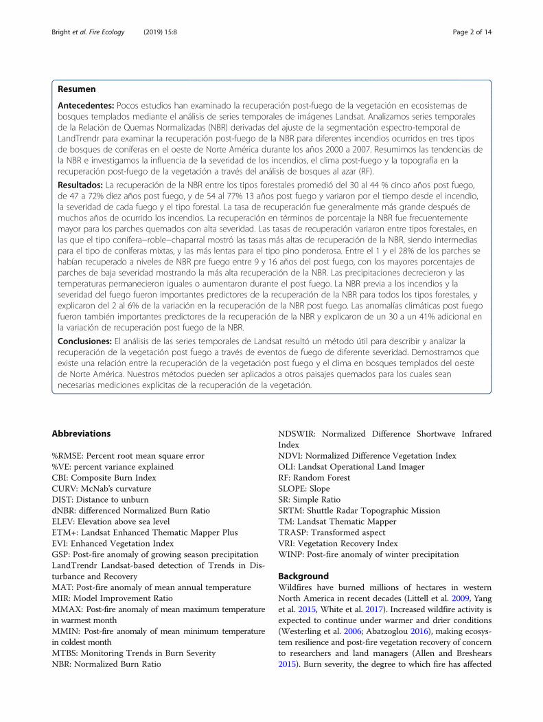
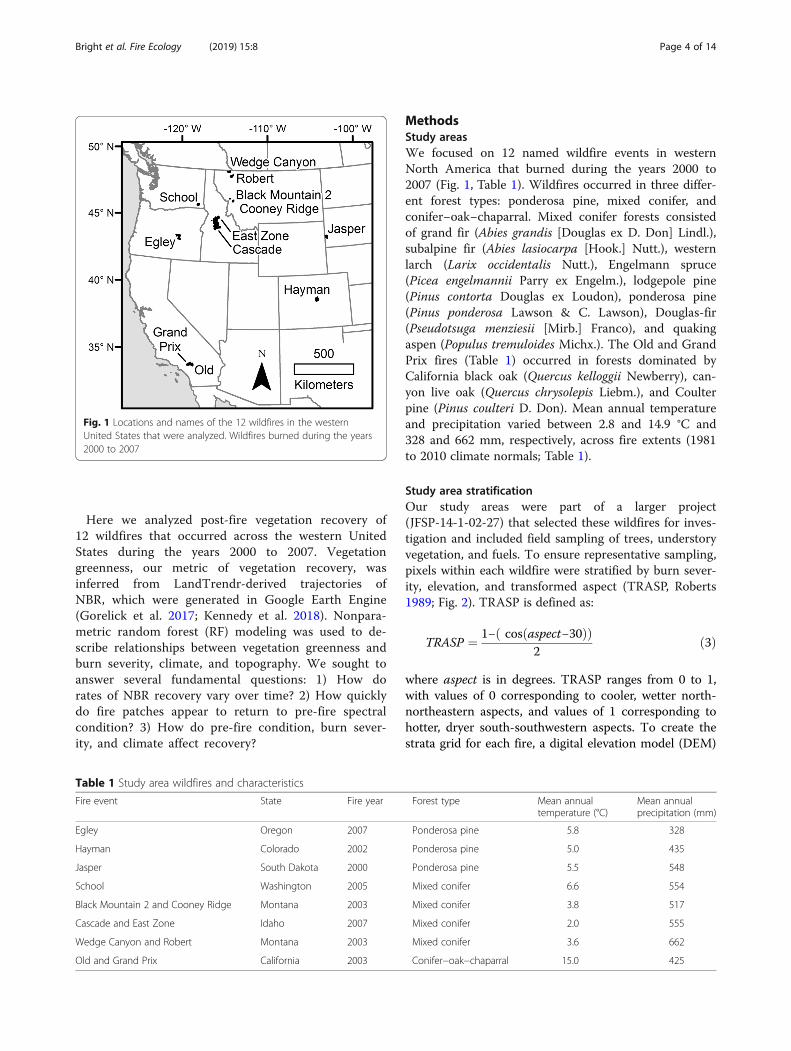
MethodsStudy areasWe focused on 12 named wildfire events in westernNorth America that burned during the years 2000 to2007 (Fig. 1, Table 1). Wildfires occurred in three differ-ent forest types: ponderosa pine, mixed conifer, andconifer−oak−chaparral. Mixed conifer forests consistedof grand fir (Abies grandis [Douglas ex D. Don] Lindl.),subalpine fir (Abies lasiocarpa [Hook.] Nutt.), westernlarch (Larix occidentalis Nutt.), Engelmann spruce(Picea engelmannii Parry ex Engelm.), lodgepole pine(Pinus contorta Douglas ex Loudon), ponderosa pine(Pinus ponderosa Lawson & C. Lawson), Douglas-fir(Pseudotsuga menziesii [Mirb.] Franco), and quakingaspen (Populus tremuloides Michx.). The Old and GrandPrix fires (Table 1) occurred in forests dominated byCalifornia black oak (Quercus kelloggii Newberry), can-yon live oak (Quercus chrysolepis Liebm.), and Coulterpine (Pinus coulteri D. Don). Mean annual temperatureand precipitation varied between 2.8 and 14.9 °C and328 and 662 mm, respectively, across fire extents (1981to 2010 climate normals; Table 1).

Study area stratificationOur study areas were part of a larger project(JFSP-14-1-02-27) that selected these wildfires for inves-tigation and included field sampling of trees, understoryvegetation, and fuels. To ensure representative sampling,pixels within each wildfire were stratified by burn sever-ity, elevation, and transformed aspect (TRASP, Roberts1989; Fig. 2). TRASP is defined as:

TRASP ¼ 1− cos aspect−30ð Þð Þ2

ð3Þ

where aspect is in degrees. TRASP ranges from 0 to 1,with values of 0 corresponding to cooler, wetter north-northeastern aspects, and values of 1 corresponding tohotter, dryer south-southwestern aspects. To create thestrata grid for each fire, a digital elevation model (DEM)

Fig. 1 Locations and names of the 12 wildfires in the westernUnited States that were analyzed. Wildfires burned during the years2000 to 2007

Table 1 Study area wildfires and characteristics

Fire event State Fire year Forest type Mean annualtemperature (°C)

Mean annualprecipitation (mm)

Egley Oregon 2007 Ponderosa pine 5.8 328

Hayman Colorado 2002 Ponderosa pine 5.0 435

Jasper South Dakota 2000 Ponderosa pine 5.5 548

School Washington 2005 Mixed conifer 6.6 554

Black Mountain 2 and Cooney Ridge Montana 2003 Mixed conifer 3.8 517

Cascade and East Zone Idaho 2007 Mixed conifer 2.0 555

Wedge Canyon and Robert Montana 2003 Mixed conifer 3.6 662

Old and Grand Prix California 2003 Conifer−oak−chaparral 15.0 425

Bright et al. Fire Ecology (2019) 15:8 Page 4 of 14

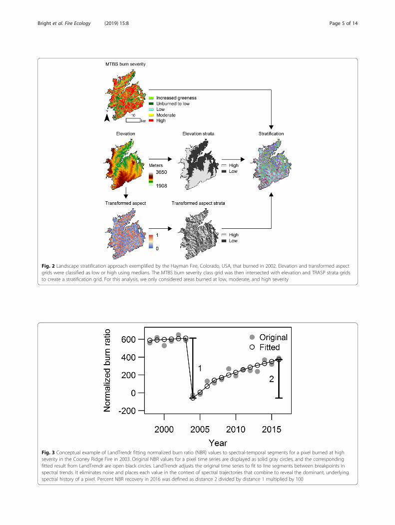
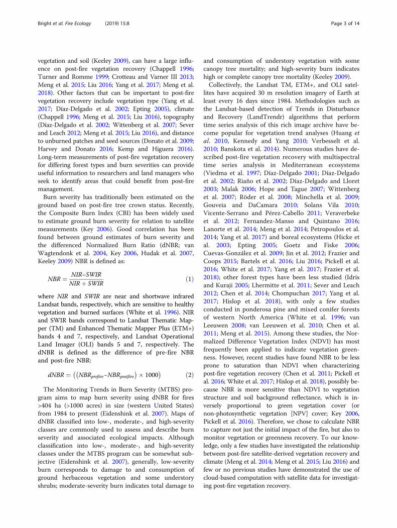
Fig. 2 Landscape stratification approach exemplified by the Hayman Fire, Colorado, USA, that burned in 2002. Elevation and transformed aspectgrids were classified as low or high using medians. The MTBS burn severity class grid was then intersected with elevation and TRASP strata gridsto create a stratification grid. For this analysis, we only considered areas burned at low, moderate, and high severity

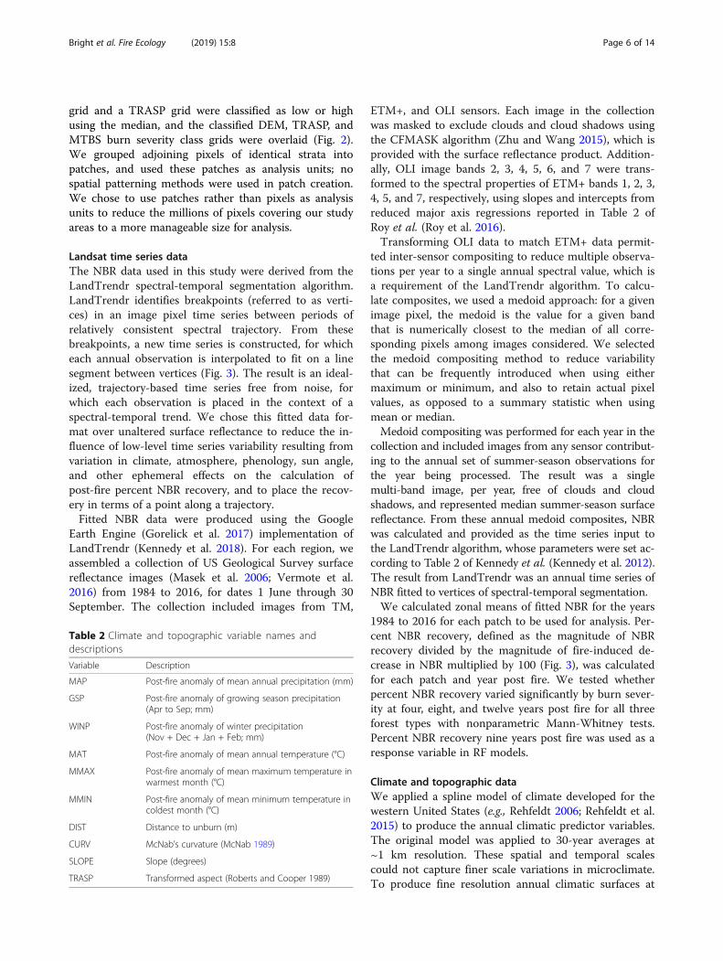
Fig. 3 Conceptual example of LandTrendr fitting normalized burn ratio (NBR) values to spectral-temporal segments for a pixel burned at highseverity in the Cooney Ridge Fire in 2003. Original NBR values for a pixel time series are displayed as solid gray circles, and the correspondingfitted result from LandTrendr are open black circles. LandTrendr adjusts the original time series to fit to line segments between breakpoints inspectral trends. It eliminates noise and places each value in the context of spectral trajectories that combine to reveal the dominant, underlyingspectral history of a pixel. Percent NBR recovery in 2016 was defined as distance 2 divided by distance 1 multiplied by 100

Bright et al. Fire Ecology (2019) 15:8 Page 5 of 14

grid and a TRASP grid were classified as low or highusing the median, and the classified DEM, TRASP, andMTBS burn severity class grids were overlaid (Fig. 2).We grouped adjoining pixels of identical strata intopatches, and used these patches as analysis units; nospatial patterning methods were used in patch creation.We chose to use patches rather than pixels as analysisunits to reduce the millions of pixels covering our studyareas to a more manageable size for analysis.

Landsat time series dataThe NBR data used in this study were derived from theLandTrendr spectral-temporal segmentation algorithm.LandTrendr identifies breakpoints (referred to as verti-ces) in an image pixel time series between periods ofrelatively consistent spectral trajectory. From thesebreakpoints, a new time series is constructed, for whicheach annual observation is interpolated to fit on a linesegment between vertices (Fig. 3). The result is an ideal-ized, trajectory-based time series free from noise, forwhich each observation is placed in the context of aspectral-temporal trend. We chose this fitted data for-mat over unaltered surface reflectance to reduce the in-fluence of low-level time series variability resulting fromvariation in climate, atmosphere, phenology, sun angle,and other ephemeral effects on the calculation ofpost-fire percent NBR recovery, and to place the recov-ery in terms of a point along a trajectory.Fitted NBR data were produced using the Google

Earth Engine (Gorelick et al. 2017) implementation ofLandTrendr (Kennedy et al. 2018). For each region, weassembled a collection of US Geological Survey surfacereflectance images (Masek et al. 2006; Vermote et al.2016) from 1984 to 2016, for dates 1 June through 30September. The collection included images from TM,

ETM+, and OLI sensors. Each image in the collectionwas masked to exclude clouds and cloud shadows usingthe CFMASK algorithm (Zhu and Wang 2015), which isprovided with the surface reflectance product. Addition-ally, OLI image bands 2, 3, 4, 5, 6, and 7 were trans-formed to the spectral properties of ETM+ bands 1, 2, 3,4, 5, and 7, respectively, using slopes and intercepts fromreduced major axis regressions reported in Table 2 ofRoy et al. (Roy et al. 2016).Transforming OLI data to match ETM+ data permit-

ted inter-sensor compositing to reduce multiple observa-tions per year to a single annual spectral value, which isa requirement of the LandTrendr algorithm. To calcu-late composites, we used a medoid approach: for a givenimage pixel, the medoid is the value for a given bandthat is numerically closest to the median of all corre-sponding pixels among images considered. We selectedthe medoid compositing method to reduce variabilitythat can be frequently introduced when using eithermaximum or minimum, and also to retain actual pixelvalues, as opposed to a summary statistic when usingmean or median.Medoid compositing was performed for each year in the

collection and included images from any sensor contribut-ing to the annual set of summer-season observations forthe year being processed. The result was a singlemulti-band image, per year, free of clouds and cloudshadows, and represented median summer-season surfacereflectance. From these annual medoid composites, NBRwas calculated and provided as the time series input tothe LandTrendr algorithm, whose parameters were set ac-cording to Table 2 of Kennedy et al. (Kennedy et al. 2012).The result from LandTrendr was an annual time series ofNBR fitted to vertices of spectral-temporal segmentation.We calculated zonal means of fitted NBR for the years

1984 to 2016 for each patch to be used for analysis. Per-cent NBR recovery, defined as the magnitude of NBRrecovery divided by the magnitude of fire-induced de-crease in NBR multiplied by 100 (Fig. 3), was calculatedfor each patch and year post fire. We tested whetherpercent NBR recovery varied significantly by burn sever-ity at four, eight, and twelve years post fire for all threeforest types with nonparametric Mann-Whitney tests.Percent NBR recovery nine years post fire was used as aresponse variable in RF models.

Climate and topographic dataWe applied a spline model of climate developed for thewestern United States (e.g., Rehfeldt 2006; Rehfeldt et al.2015) to produce the annual climatic predictor variables.The original model was applied to 30-year averages at~1 km resolution. These spatial and temporal scalescould not capture finer scale variations in microclimate.To produce fine resolution annual climatic surfaces at

Table 2 Climate and topographic variable names anddescriptions

Variable Description

MAP Post-fire anomaly of mean annual precipitation (mm)

GSP Post-fire anomaly of growing season precipitation(Apr to Sep; mm)

WINP Post-fire anomaly of winter precipitation(Nov + Dec + Jan + Feb; mm)

MAT Post-fire anomaly of mean annual temperature (°C)

MMAX Post-fire anomaly of mean maximum temperature inwarmest month (°C)

MMIN Post-fire anomaly of mean minimum temperature incoldest month (°C)

DIST Distance to unburn (m)

CURV McNab’s curvature (McNab 1989)

SLOPE Slope (degrees)

TRASP Transformed aspect (Roberts and Cooper 1989)

Bright et al. Fire Ecology (2019) 15:8 Page 6 of 14

30 m resolution, we applied the model to annual cli-matic data for the years 1981 to 2010 using the digitalelevation model from the Shuttle Radar TopographicMission (SRTM). We used the ANUSPLIN program forthin plate spline interpolation of climatic variables(Hutchinson 2000). We then derived additional climaticindices and interactive variables from the original sur-face variables created by the model.Climate variable indices were converted to post-fire

climate anomaly grids because we were interested inhow post-fire climate affected vegetation recovery, andso that across-fire climate comparisons could be made(Arnold et al. 2014; Meng et al. 2015; Liu 2016). Anom-alies were calculated using the Z-statistic:

Z ¼ μpost−μnormσ

ð4Þ

where μpost is the post-fire mean (one year post fire to2010), μnorm is the climate normal (1984 to 2010) mean,and σ is the climate normal standard deviation; the re-sult was one mean anomaly grid for each climate vari-able. Post-fire means ended at 2010 because that was thelast year of available climate data.Topographic variable grids were derived from DEMs

of each fire extent (Table 2). McNab’s curvature was cal-culated using the spatialEco package in R (McNab 1989;R Core Team 2017; Evans 2017), and is a measure ofslope shape, whether convex or concave. Curvature canaffect soil moisture, erosion, and deposition, and thusvegetation growth. Distance to unburned was calculatedas the shortest distance to the fire perimeter or an un-burned patch. We calculated zonal means of climateanomalies and topographic variables for each patch tobe used for RF analysis. Raster processing was per-formed in R using the raster package (Hijmans 2016; RCore Team 2017).

Random forest analysisWe explored the relationship between climate, topog-raphy, and post-fire NBR recovery by relating percentNBR recovery nine years post fire to post-fire climateanomaly and topographic variables (Table 2) via randomforest (RF) modeling, implemented in R (Breiman 2001;Liaw 2002; R Core Team 2017). We chose to use anonparametric modeling method because most variabledistributions were non-normal and caused visibly non-random trends in residuals of initial linear models. RFmodeling does not require variables to be normallydistributed, can handle tens of thousands of cases, andprovides variable importance scores.We created RF models for each forest type using three

different sets of explanatory variables to investigate howclimate and topographic variables contributed to

explaining variance in NBR recovery. Initial RF modelsincluded only pre-fire NBR (indicator of pre-fire vegeta-tion cover) and dNBR (burn severity) as explanatory var-iables. Post-fire climate explanatory variables were thenadded and additional RF models were created, and fi-nally topography variables were added as explanatoryvariables. We were computationally unable to create anRF model with all 263 449 mixed conifer patches; there-fore, we created 10 models using 10% samples of themixed conifer patches, and averaged model results. RFmodels were evaluated with percent root mean squareerror (%RMSE) and percent variance explained (%VE) inpercent NBR recovery, calculated as:

%RMSE ¼ffiffiffiffiffiffiffiffiffiffiMSE

p

NBRrec� 100 ð5Þ

%VE ¼ 1−MSEvar NBRrecð Þ � 100 ð6Þ

where MSE is the mean square error, the sum of squaredresiduals divided by n, and NBRrec is percent NBR recov-ery. For RF models that included all explanatory variables,we calculated the model improvement ratio (MIR), astandardized measure of variable importance rangingbetween 0 and 1, for each variable (Murphy and Ev-ans 2010). MIR measures were advantageous to rawimportance scores because they were comparable be-tween RF models. A MIR score of 1 indicated mostimportant, 0 least important.

ResultsPatch statisticsWe examined a total of 435 367 patches of variable size(Table 3). Patch size averaged 0.67 ha and ranged from0.09 to 683.73 ha. Minimum and median patch sizeswere one and two pixels, respectively. The Cascade andEast Zone fires were the largest fires analyzed; the BlackMountain 2, Cooney Ridge, and School fires were thesmallest fires analyzed.

Vegetation recoveryNBR recovery rates varied non-linearly by time since fire(Fig. 4, Additional file 1). The rate of NBR recovery wasgreatest several years following fire, after which it de-creased. Patches that burned at high severity generallyshowed the greatest recovery, especially for the mixedconifer forest type. For ponderosa pine, patches thatburned at moderate and high severity began to show lessrecovery than patches that burned at low severity, begin-ning 13 years post fire. Percent NBR recovery differedsignificantly by burn severity at four, eight, and twelveyears post fire (considered representative of the recoverytrends) for all three forest types (Mann-Whitney tests, P< 0.001); large sample sizes (Table 3) gave statistical tests

Bright et al. Fire Ecology (2019) 15:8 Page 7 of 14

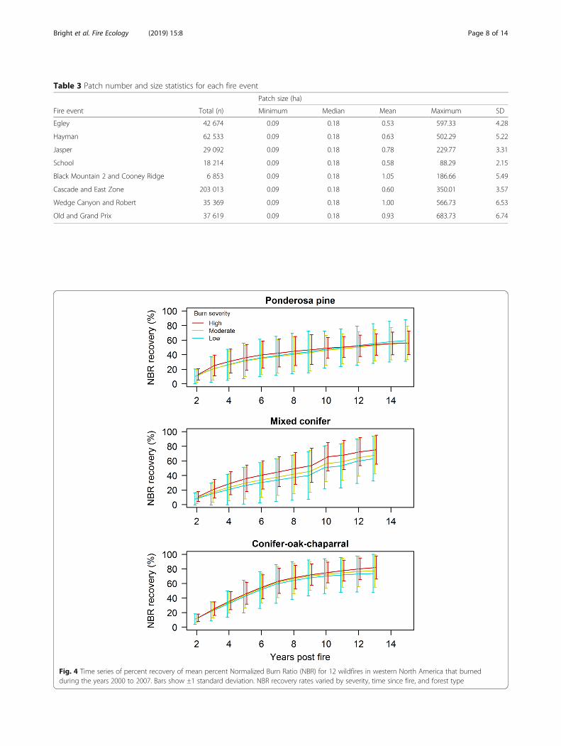
Fig. 4 Time series of percent recovery of mean percent Normalized Burn Ratio (NBR) for 12 wildfires in western North America that burnedduring the years 2000 to 2007. Bars show ±1 standard deviation. NBR recovery rates varied by severity, time since fire, and forest type

Table 3 Patch number and size statistics for each fire event

Patch size (ha)

Fire event Total (n) Minimum Median Mean Maximum SD

Egley 42 674 0.09 0.18 0.53 597.33 4.28

Hayman 62 533 0.09 0.18 0.63 502.29 5.22

Jasper 29 092 0.09 0.18 0.78 229.77 3.31

School 18 214 0.09 0.18 0.58 88.29 2.15

Black Mountain 2 and Cooney Ridge 6 853 0.09 0.18 1.05 186.66 5.49

Cascade and East Zone 203 013 0.09 0.18 0.60 350.01 3.57

Wedge Canyon and Robert 35 369 0.09 0.18 1.00 566.73 6.53

Old and Grand Prix 37 619 0.09 0.18 0.93 683.73 6.74

Bright et al. Fire Ecology (2019) 15:8 Page 8 of 14

considerable power so that even small differences weresignificant (Fig. 4).The rate of NBR recovery was smallest in the ponder-

osa pine forest type, intermediate in the mixed coniferforest type, and greatest in the conifer−oak−chaparralforest type (Fig. 4, Table 4). Recovery patterns for eachfire event reflected this pattern, although individual firesshowed some unique patterns as well (Additional file 1).Most patches had not completely recovered to pre-fire

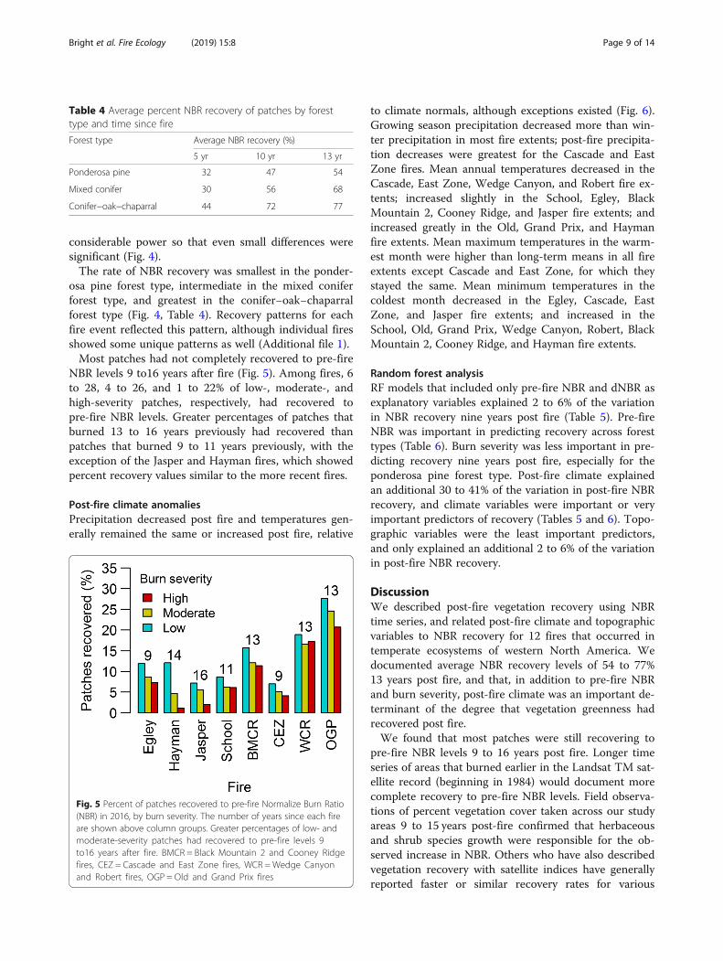
NBR levels 9 to16 years after fire (Fig. 5). Among fires, 6to 28, 4 to 26, and 1 to 22% of low-, moderate-, andhigh-severity patches, respectively, had recovered topre-fire NBR levels. Greater percentages of patches thatburned 13 to 16 years previously had recovered thanpatches that burned 9 to 11 years previously, with theexception of the Jasper and Hayman fires, which showedpercent recovery values similar to the more recent fires.

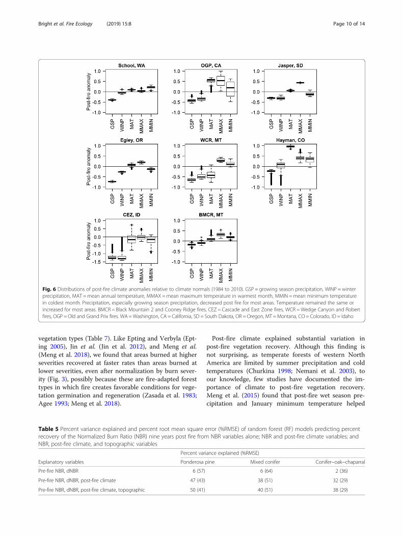
Post-fire climate anomaliesPrecipitation decreased post fire and temperatures gen-erally remained the same or increased post fire, relative

to climate normals, although exceptions existed (Fig. 6).Growing season precipitation decreased more than win-ter precipitation in most fire extents; post-fire precipita-tion decreases were greatest for the Cascade and EastZone fires. Mean annual temperatures decreased in theCascade, East Zone, Wedge Canyon, and Robert fire ex-tents; increased slightly in the School, Egley, BlackMountain 2, Cooney Ridge, and Jasper fire extents; andincreased greatly in the Old, Grand Prix, and Haymanfire extents. Mean maximum temperatures in the warm-est month were higher than long-term means in all fireextents except Cascade and East Zone, for which theystayed the same. Mean minimum temperatures in thecoldest month decreased in the Egley, Cascade, EastZone, and Jasper fire extents; and increased in theSchool, Old, Grand Prix, Wedge Canyon, Robert, BlackMountain 2, Cooney Ridge, and Hayman fire extents.

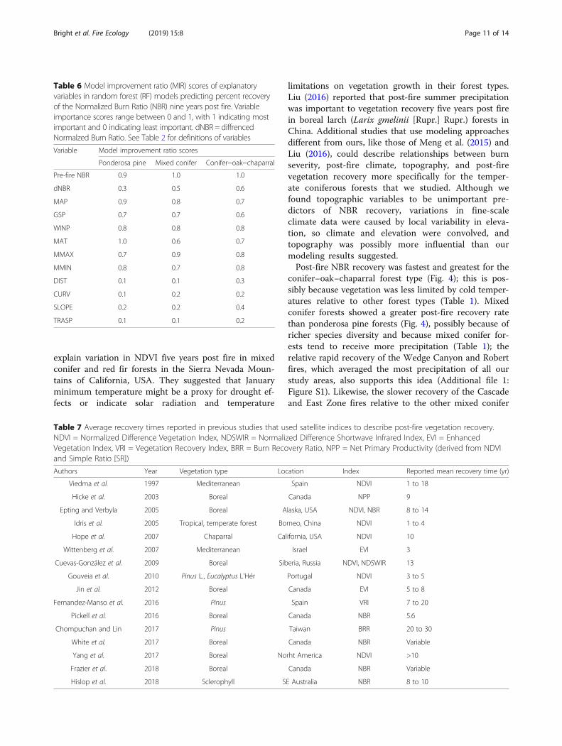
Random forest analysisRF models that included only pre-fire NBR and dNBR asexplanatory variables explained 2 to 6% of the variationin NBR recovery nine years post fire (Table 5). Pre-fireNBR was important in predicting recovery across foresttypes (Table 6). Burn severity was less important in pre-dicting recovery nine years post fire, especially for theponderosa pine forest type. Post-fire climate explainedan additional 30 to 41% of the variation in post-fire NBRrecovery, and climate variables were important or veryimportant predictors of recovery (Tables 5 and 6). Topo-graphic variables were the least important predictors,and only explained an additional 2 to 6% of the variationin post-fire NBR recovery.

DiscussionWe described post-fire vegetation recovery using NBRtime series, and related post-fire climate and topographicvariables to NBR recovery for 12 fires that occurred intemperate ecosystems of western North America. Wedocumented average NBR recovery levels of 54 to 77%13 years post fire, and that, in addition to pre-fire NBRand burn severity, post-fire climate was an important de-terminant of the degree that vegetation greenness hadrecovered post fire.We found that most patches were still recovering to

pre-fire NBR levels 9 to 16 years post fire. Longer timeseries of areas that burned earlier in the Landsat TM sat-ellite record (beginning in 1984) would document morecomplete recovery to pre-fire NBR levels. Field observa-tions of percent vegetation cover taken across our studyareas 9 to 15 years post-fire confirmed that herbaceousand shrub species growth were responsible for the ob-served increase in NBR. Others who have also describedvegetation recovery with satellite indices have generallyreported faster or similar recovery rates for various

Table 4 Average percent NBR recovery of patches by foresttype and time since fire

Forest type Average NBR recovery (%)

5 yr 10 yr 13 yr

Ponderosa pine 32 47 54

Mixed conifer 30 56 68

Conifer−oak−chaparral 44 72 77

Fig. 5 Percent of patches recovered to pre-fire Normalize Burn Ratio(NBR) in 2016, by burn severity. The number of years since each fireare shown above column groups. Greater percentages of low- andmoderate-severity patches had recovered to pre-fire levels 9to16 years after fire. BMCR = Black Mountain 2 and Cooney Ridgefires, CEZ = Cascade and East Zone fires, WCR = Wedge Canyonand Robert fires, OGP = Old and Grand Prix fires

Bright et al. Fire Ecology (2019) 15:8 Page 9 of 14

vegetation types (Table 7). Like Epting and Verbyla (Ept-ing 2005), Jin et al. (Jin et al. 2012), and Meng et al.(Meng et al. 2018), we found that areas burned at higherseverities recovered at faster rates than areas burned atlower severities, even after normalization by burn sever-ity (Fig. 3), possibly because these are fire-adapted foresttypes in which fire creates favorable conditions for vege-tation germination and regeneration (Zasada et al. 1983;Agee 1993; Meng et al. 2018).

Post-fire climate explained substantial variation inpost-fire vegetation recovery. Although this finding isnot surprising, as temperate forests of western NorthAmerica are limited by summer precipitation and coldtemperatures (Churkina 1998; Nemani et al. 2003), toour knowledge, few studies have documented the im-portance of climate to post-fire vegetation recovery.Meng et al. (2015) found that post-fire wet season pre-cipitation and January minimum temperature helped

Fig. 6 Distributions of post-fire climate anomalies relative to climate normals (1984 to 2010). GSP = growing season precipitation, WINP = winterprecipitation, MAT =mean annual temperature, MMAX =mean maximum temperature in warmest month, MMIN =mean minimum temperaturein coldest month. Precipitation, especially growing season precipitation, decreased post fire for most areas. Temperature remained the same orincreased for most areas. BMCR = Black Mountain 2 and Cooney Ridge fires, CEZ = Cascade and East Zone fires, WCR =Wedge Canyon and Robertfires, OGP = Old and Grand Prix fires. WA=Washington, CA = California, SD = South Dakota, OR = Oregon, MT =Montana, CO = Colorado, ID = Idaho

Table 5 Percent variance explained and percent root mean square error (%RMSE) of random forest (RF) models predicting percentrecovery of the Normalized Burn Ratio (NBR) nine years post fire from NBR variables alone; NBR and post-fire climate variables; andNBR, post-fire climate, and topographic variables

Percent variance explained (%RMSE)

Explanatory variables Ponderosa pine Mixed conifer Conifer−oak−chaparral

Pre-fire NBR, dNBR 6 (57) 6 (64) 2 (36)

Pre-fire NBR, dNBR, post-fire climate 47 (43) 38 (51) 32 (29)

Pre-fire NBR, dNBR, post-fire climate, topographic 50 (41) 40 (51) 38 (29)

Bright et al. Fire Ecology (2019) 15:8 Page 10 of 14

explain variation in NDVI five years post fire in mixedconifer and red fir forests in the Sierra Nevada Moun-tains of California, USA. They suggested that Januaryminimum temperature might be a proxy for drought ef-fects or indicate solar radiation and temperature

limitations on vegetation growth in their forest types.Liu (2016) reported that post-fire summer precipitationwas important to vegetation recovery five years post firein boreal larch (Larix gmelinii [Rupr.] Rupr.) forests inChina. Additional studies that use modeling approachesdifferent from ours, like those of Meng et al. (2015) andLiu (2016), could describe relationships between burnseverity, post-fire climate, topography, and post-firevegetation recovery more specifically for the temper-ate coniferous forests that we studied. Although wefound topographic variables to be unimportant pre-dictors of NBR recovery, variations in fine-scaleclimate data were caused by local variability in eleva-tion, so climate and elevation were convolved, andtopography was possibly more influential than ourmodeling results suggested.Post-fire NBR recovery was fastest and greatest for the

conifer−oak−chaparral forest type (Fig. 4); this is pos-sibly because vegetation was less limited by cold temper-atures relative to other forest types (Table 1). Mixedconifer forests showed a greater post-fire recovery ratethan ponderosa pine forests (Fig. 4), possibly because ofricher species diversity and because mixed conifer for-ests tend to receive more precipitation (Table 1); therelative rapid recovery of the Wedge Canyon and Robertfires, which averaged the most precipitation of all ourstudy areas, also supports this idea (Additional file 1:Figure S1). Likewise, the slower recovery of the Cascadeand East Zone fires relative to the other mixed conifer

Table 6 Model improvement ratio (MIR) scores of explanatoryvariables in random forest (RF) models predicting percent recoveryof the Normalized Burn Ratio (NBR) nine years post fire. Variableimportance scores range between 0 and 1, with 1 indicating mostimportant and 0 indicating least important. dNBR = diffrencedNormalzed Burn Ratio. See Table 2 for definitions of variables

Variable Model improvement ratio scores

Ponderosa pine Mixed conifer Conifer−oak−chaparral

Pre-fire NBR 0.9 1.0 1.0

dNBR 0.3 0.5 0.6

MAP 0.9 0.8 0.7

GSP 0.7 0.7 0.6

WINP 0.8 0.8 0.8

MAT 1.0 0.6 0.7

MMAX 0.7 0.9 0.8

MMIN 0.8 0.7 0.8

DIST 0.1 0.1 0.3

CURV 0.1 0.2 0.2

SLOPE 0.2 0.2 0.4

TRASP 0.1 0.1 0.2

Table 7 Average recovery times reported in previous studies that used satellite indices to describe post-fire vegetation recovery.NDVI = Normalized Difference Vegetation Index, NDSWIR = Normalized Difference Shortwave Infrared Index, EVI = EnhancedVegetation Index, VRI = Vegetation Recovery Index, BRR = Burn Recovery Ratio, NPP = Net Primary Productivity (derived from NDVIand Simple Ratio [SR])

Authors Year Vegetation type Location Index Reported mean recovery time (yr)

Viedma et al. 1997 Mediterranean Spain NDVI 1 to 18

Hicke et al. 2003 Boreal Canada NPP 9

Epting and Verbyla 2005 Boreal Alaska, USA NDVI, NBR 8 to 14

Idris et al. 2005 Tropical, temperate forest Borneo, China NDVI 1 to 4

Hope et al. 2007 Chaparral California, USA NDVI 10

Wittenberg et al. 2007 Mediterranean Israel EVI 3

Cuevas-González et al. 2009 Boreal Siberia, Russia NDVI, NDSWIR 13

Gouveia et al. 2010 Pinus L., Eucalyptus L’Hér Portugal NDVI 3 to 5

Jin et al. 2012 Boreal Canada EVI 5 to 8

Fernandez-Manso et al. 2016 Pinus Spain VRI 7 to 20

Pickell et al. 2016 Boreal Canada NBR 5.6

Chompuchan and Lin 2017 Pinus Taiwan BRR 20 to 30

White et al. 2017 Boreal Canada NBR Variable

Yang et al. 2017 Boreal Norht America NDVI >10

Frazier et al. 2018 Boreal Canada NBR Variable

Hislop et al. 2018 Sclerophyll SE Australia NBR 8 to 10

Bright et al. Fire Ecology (2019) 15:8 Page 11 of 14

areas might have been due to greater relative decreasesin post-fire precipitation (Additional file 1, Fig. 6).We used recovery of NBR, a satellite index, as an indica-

tor of vegetation recovery. Although satellite observationscontain valuable information about vegetation conditions,they are simply measurements of reflected light and aretherefore limited in their interpretability. NBR is an indi-cation of the ratio of vegetation to soil cover, but tells uslittle about vegetation type and structure. Relating groundand satellite observations can increase interpretability ofsatellite observations (Hudak et al. 2007), as well as pro-vide a means for applying spatially limited ground obser-vations across landscapes. We chose to limit this analysisto NBR observations because we wished to describelandscape-wide vegetation recovery in general. Futurestudies that predict ground-measured vegetation charac-teristics from time series of multispectral imagery coulddescribe post-fire recovery trajectories of more specificvegetation characteristics.

ConclusionsLandsat time series analysis can provide landscape-wideinformation on post-fire vegetation recovery. Ouranalysis revealed that complete post-fire recovery ofNBR in the temperate forest ecosystems of westernNorth America takes longer than 9 to 16 years for mostareas. We found burn severity, pre-fire NBR, and post-fireclimate to be important to vegetation recovery for the firesthat we studied. Methods similar to ours could be appliedto other burned areas for which landscape-wide informa-tion on post-disturbance vegetation recovery is needed,and could be used to inform management decisions; forinstance, individual patches showing little or no recoverycould be identified for post-fire management. Our findingthat post-fire climate influences vegetation recovery sug-gests that climate change will affect post-fire vegetationrecovery in western North America.

Additional file

Additional file 1: Time series of percent recovery of mean percentNormalized Burn Ratio (NBR) by burn severity for each fire. Bars show ±1standard deviation. NBR recovery rates varied by fire, severity, time sincefire, and forest type. Forest type, year of fire, mean average temperature(°C), and mean annual precipitation (mm) are given in the upperleft-hand corner of each panel. (TIF 457 kb)

AcknowledgementsThe authors thank three anonymous reviewers for their time and helpfulreviews.

FundingResearch was funded by the Joint Fire Science Program (JFSP-14-1-02-27).

Availability of data and materialsThe datasets used and analyzed during the current study are available fromthe corresponding author on reasonable request.

Authors’ contributionsBB and AH conceived and designed the analysis; BB performed theanalysis; RK and JB provided Landsat time series data. AHK providedclimate data. BB, AH, RK, JB, and AHK wrote the manuscript. All authorsread and approved the final manuscript.

Ethics approval and consent to participateNot applicable.

Consent for publicationNot applicable.

Competing interestsThe authors declare that they have no competing interests.

Publisher’s NoteSpringer Nature remains neutral with regard to jurisdictional claims in publishedmaps and institutional affiliations.

Author details1USDA Forest Service, Rocky Mountain Research Station, 1221 S. Main Street,Moscow, Idaho 83843, USA. 2Oregon State University, College of Earth,Ocean, and Atmospheric Sciences, 104 CEOAS Administration Building, 101SW 26th Street, Corvallis, Oregon 97331, USA. 3Natural Resource EcologyLaboratory, Colorado State University, NESB Building, 1499 Campus Delivery,A215, Fort Collins, Colorado 80523, USA.

Received: 1 June 2018 Accepted: 18 November 2018

ReferencesAbatzoglou, J.T., and A.P. Williams. 2016. Impact of anthropogenic climate

change on wildfire across western US forests. PNAS 113: 11770–11775.https://doi.org/10.1073/pnas.1607171113.

Agee, J.K. 1993. Fire ecology of Pacific Northwest forests. Washington, D.C: IslandPress.

Allen, C.D., D.D. Breshears, and N.G. McDowell. 2015. On underestimation ofglobal vulnerability to tree mortality and forest die-off from hotterdrought in the Anthropocene. Ecosphere 6: 1–55. https://doi.org/10.1890/ES15-00203.1.

Arnold, J.D., S.C. Brewer, and P.E. Dennison. 2014. Modeling climate-fireconnections within the Great Basin and Upper Colorado River Basin, westernUnited States. Fire Ecology 10: 64–75. https://doi.org/10.4996/fireecology.1002064.

Banskota, A., N. Kayastha, M.J. Falkowski, M.A. Wulder, R.E. Froese, and J.C. White.2014. Forest monitoring using Landsat time series data: a review. CanadianJournal of Remote Sensing 40: 3623–3684. https://doi.org/10.1080/07038992.2014.987376.

Bartels, S.F., H.Y.H. Chen, M.A. Wulder, and J.C. White. 2016. Trends in post-disturbance recovery rates of Canada’s forests following wildfire and harvest.Forest Ecology and Management 361: 194–207. https://doi.org/10.1016/j.foreco.2015.11.015.

Breiman, L. 2001. Random forests. Machine Learning 45: 5–32. https://doi.org/10.1023/A:1010933404324.

Chappell, C.B., and J.K. Agee. 1996. Fire severity and tree seedling establishmentin Abies magnifica forests, southern Cascades, Oregon. Ecological Applications6: 628–640. https://doi.org/10.2307/2269397.

Chen, W., K. Moriya, T. Sakai, L. .Koyama, and C. Cao. 2014. Monitoring of post-fireforest recovery under different restoration modes based on time seriesLandsat data. European Journal of Remote Sensing 47: 153–168. https://doi.org/10.5721/EuJRS20144710.

Chen, X., J.E. Vogelmann, M. Rollins, D. Ohlen, C.H. Key, L. Yang, C. Huang, and H.Shi. 2011. Detecting post-fire burn severity and vegetation recovery usingmultitemporal remote sensing spectral indices and field-collected compositeburn index data in a ponderosa pine forest. International Journal of RemoteSensing 32: 7905–7927. https://doi.org/10.1080/01431161.2010.524678.

Chompuchan, C., and C.Y. Lin. 2017. Assessment of forest recovery at Wu-Lingfire scars in Taiwan using multi-temporal Landsat imagery. EcologicalIndicators 79: 196–206. https://doi.org/10.1016/j.ecolind.2017.04.038.

Bright et al. Fire Ecology (2019) 15:8 Page 12 of 14

Churkina, G., and S.W. Running. 1998. Contrasting climatic controls on theestimated productivity of global terrestrial biomes. Ecosystems 1: 206–215.https://doi.org/10.1007/s100219900016.

Crotteau, J.S., J.M. Varner III, and M.W. Ritchie. 2013. Post-fire regeneration acrossa fire severity gradient in the southern Cascades. Forest Ecology andManagement 287: 103–112. https://doi.org/10.1016/j.foreco.2012.09.022.

Cuevas-González, M., F. Gerard, H. Balzter, and D. Riaño. 2009. Analysing forestrecovery after wildfire disturbance in boreal Siberia using remotely sensedvegetation indices. Global Change Biology 15: 561–577. https://doi.org/10.1111/j.1365-2486.2008.01784.x.

Díaz-Delgado, R., and X. Pons. 2001. Spatial patterns of forest fires in Catalonia(NE of Spain) along the period 1975-1995: analysis of vegetation recoveryafter fire. Forest Ecology and Management 147: 67–74. https://doi.org/10.1016/S0378-1127(00)00434-5.

Díaz-Delgado, R., F. Lloret, and X. Pons. 2003. Influence of fire severity on plantregeneration by means of remote sensing imagery. International Journal ofRemote Sensing 24: 1751–1763. https://doi.org/10.1080/01431160210144732.

Díaz-Delgado, R., F. Lloret, X. Pons, and J. Terradas. 2002. Satellite evidence ofdecreasing resilience in Mediterranean plant communities after recurrentwildfires. Ecology 83: 2293–2303.

Donato, D.C., J.B. Fontaine, J.L. Campbell, W.D. Robinson, J.B. Kauffman, and B.E.Law. 2009. Conifer regeneration in stand-replacement portions of a largemixed-severity wildfire in the Klamath-Siskiyou Mountains. Canadian Journalof Forest Research 39: 823–838. https://doi.org/10.1139/X09-016.

Eidenshink, J., B. Schwind, K. Brewer, Z. Zhu, B. Quayle, and S. Howard. 2007. Aproject for monitoring trends in burn severity. Fire Ecology 3: 3–21. https://doi.org/10.4996/fireecology.0301003.

Epting, J., and J. Verbyla. 2005. Landscape-level interactions of prefire vegetation, burnseverity, and postfire vegetation over a 16-year period in interior Alaska. CanadianJournal of Forest Research 35: 1367–1377. https://doi.org/10.1139/X05-060.

Evans, J.S. 2017. spatialEco. R package version 0.0.1-7. https://CRAN.R-project.org/package=spatialEco. Accessed January 2018

Fernandez-Manso, A., C. Quintano, and D.A. Roberts. 2016. Burn severity influenceon post-fire vegetation cover resilience from Landsat MESMA fraction imagestime series in Mediterranean forest ecosystems. Remote Sensing ofEnvironment 184: 112–123. https://doi.org/10.1016/j.rse.2016.06.015.

Frazier, R.J., N.C. .Coops, M.A. Wulder, T. Hermosilla, and J.C. White. 2018.Analyzing spatial and temporal variability in short-term rates of post-firevegetation return from Landsat time series. Remote Sensing of Environment205: 32–45. https://doi.org/10.1016/j.rse.2017.11.007.

Frazier, R.J., N.C. Coops, and M.A. Wulder. 2015. Boreal Shield forest disturbanceand recovery trends using Landsat time series. Remote Sensing ofEnvironment 170: 317–327. https://doi.org/10.1016/j.rse.2015.09.015.

Goetz, S.J., G.J. Fiske, and A.G. Bunn. 2006. Using satellite time-series data sets toanalyze fire disturbance and forest recovery across Canada. Remote Sensing ofEnvironment 101: 352–365. https://doi.org/10.1016/j.rse.2006.01.011.

Gorelick, N., M. Hancher, M. Dixon, S. Ilyushchenko, D. Thau, and R. Moore. 2017.Google Earth Engine: planetary-scale geospatial analysis for everyone. RemoteSensing of Environment 202: 18–27. https://doi.org/10.1016/j.rse.2017.06.031.

Gouveia, C., C.C. DaCamara, and R.M. Trigo. 2010. Post-fire vegetation recovery inPortugal based on spot/vegetation data. Natural Hazards and Earth SystemSciences 10: 673–684. https://doi.org/10.5194/nhess-10-673-2010.

Harvey, B.J., D.C. Donato, and M.G. Turner. 2016. High and dry: post-fire treeseedling establishment in subalpine forests decreases with post-fire droughtand large stand-replacing burn patches. Global Ecology and Biogeography 25:655–669. https://doi.org/10.1111/geb.12443.

Hicke, J.A., G.P. Asner, E.S. Kasischke, N.H.F. French, J.T. Randerson, G.J. Collatz, B.J. Stocks, C.J. Tucker, S.O. Los, and C.B. Field. 2003. Postfire response of North American borealforest net primary productivity analyzed with satellite observations. Global ChangeBiology 9: 1145–1157. https://doi.org/10.1046/j.1365-2486.2003.00658.x.

Hijmans, R.J. 2016. raster: geographic data analysis and modeling. R package version2: 5–8 https://CRAN.R-project.org/package=raster. Accessed January 2018.

Hislop, S., S. Jones, M. Soto-Berelov, A. Skidmore, A. .Haywood, and T.H. Nguyen.2018. Using Landsat spectral indices in time-series to assess wildfire disturbanceand recovery. Remote Sensing 10: 460. https://doi.org/10.3390/rs10030460.

Hope, A., C. Tague, and R. Clark. 2007. Characterizing post-fire vegetationrecovery of California chaparral using TM/ETM+ time-series data. InternationalJournal of Remote Sensing 28: 1339–1354. https://doi.org/10.1080/01431160600908924.

Huang, C., S.N. Goward, J.G. Masek, N. Thomas, Z. Zhu, and J.E. Vogelmann. 2010.An automated approach for reconstructing recent forest disturbance history

using dense Landsat time series stacks. Remote Sensing of Environment 114:183–198. https://doi.org/10.1016/j.rse.2009.08.017.

Hudak, A.T., P. Morgan, M.J. Bobbitt, A.M.S. Smith, S.A. Lewis, L.B. Lentile, P.R.Robichaud, J.T. Clark, and R.A. McKinley. 2007. The relationship ofmultispectral satellite imagery to immediate fire effects. Fire Ecology 3: 64–90.https://doi.org/10.4996/fireecology.0301064.

Hutchinson, M.F. 2000. ANUSPLIN user guide version 4.1. Centre for Resource andEnvironmental Studies. Canberra: Australian National University.

Idris, M.H., K. Kuraji, and M. Suzuki. 2005. Evaluating vegetation recovery followinglarge-scale forest fires in Borneo and northeastern China using multi-temporal NOAA/AVHRR images. Journal of Forest Research 10: 101–111.https://doi.org/10.1007/s10310-004-0106-y.

Jin, Y., J.T. Randerson, S.J. Goetz, P.S.A. Beck, M.M. Loranty, and M.L. Goulden. 2012.The influence of burn severity on postfire vegetation recovery and albedochange during early succession in North American boreal forests. Journal ofGeophysical Research 117: G01036. https://doi.org/10.1029/2011JG001886.

Keeley, J.E. 2009. Fire intensity, fire severity and burn severity: a brief review andsuggested usage. International Journal of Wildland Fire 18: 116–126. https://doi.org/10.1071/WF07049.

Kemp, K.B., P.E. Higuera, and P. Morgan. 2016. Fire legacies impact coniferregeneration across environmental gradients in the US northern Rockies.Landscape Ecology 31: 619. https://doi.org/10.1007/s10980-015-0268-3.

Kennedy, R.E., Z. Yang, W.B. Cohen, E. Pfaff, J. Braaten, and P. Nelson. 2012. Spatialand temporal patterns of forest disturbance and regrowth within the area ofthe Northwest Forest Plan. Remote Sensing of Environment 122: 117–133.https://doi.org/10.1016/j.rse.2011.09.024.

Kennedy, R.E., Z. Yang, N. Gorelick, J. Braaten, L. Cavalcante, W.B. Cohen, and S.Healey. 2018. Implementation of the LandTrendr algorithm on Google EarthEngine. Remote Sensing 10: 691. https://doi.org/10.3390/rs10050691.

Kennedy, R.E., Z.G. Yang, and W.B. Cohen. 2010. Detecting trends in forestdisturbance and recovery using yearly Landsat time series: 1. LandTrendr-temporal segmentation algorithms. Remote Sensing of Environment 114:2897–2910. https://doi.org/10.1016/j.rse.2010.07.008.

Key, C.H., and N.C. Benson. 2006. Landscape assessment: ground measure of severity,the Composite Burn Index; and remote sensing of severity, the Normalized BurnRatio. Pages LA1-LA51. In FIREMON: fire effects monitoring and inventory system,ed. D.C. Lutes, R.E. Keane, J.F. Caratti, C.H. Key, N.C. Benson, S. Sutherland, and L.J.Gangi. Fort Collins: USDA Forest Service General Technical Report RMRS-GTR-164-CD, Rocky Mountain Research Station.

Lanorte, A., R. Lasaponara, M. Lovallo, and L. Telesca. 2014. Fisher-Shannoninformation plane analysis of SPOT/VEGETATION Normalized DifferenceVegetation Index (NDVI) time series to characterize vegetation recovery afterfire disturbance. International Journal of Applied Earth Observation andGeoinformation 26: 441–446. https://doi.org/10.1016/j.jag.2013.05.008.

Lhermitte, S., J. Verbesselt, W.W. Verstraeten, S. Veraverbeke, and P. Coppin. 2011.Assessing intra-annual vegetation regrowth after fire using the pixel basedregeneration index. ISPRS Journal of Photogrammetry and Remote Sensing 66:17–27. https://doi.org/10.1016/j.isprsjprs.2010.08.004.

Liaw, A., and M. Wiener. 2002. Classification and regression by randomForest. RNews 2: 18–22 https://cran.r-project.org/doc/Rnews/Rnews_2002-3.pdf.Accessed Jan 2018.

Littell, J.S., D. McKenzie, D.L. Peterson, and A.L. Westerling. 2009. Climate andwildfire area burned in western US ecoprovinces, 1916-2003. EcologicalApplications 19: 1003–1021. https://doi.org/10.1890/07-1183.1.

Liu, Z. 2016. Effects of climate and fire on short-term vegetation recovery in theboreal larch forests of northeastern China. Scientific Reports 6: 37572. https://doi.org/10.1038/srep37572.

Malak, D.A., and J.G. Pausas. 2006. Fire regime and post-fire NormalizedDifference Vegetation Index changes in the eastern Iberian peninsula(Mediterranean Basin). International Journal of Wildland Fire 15: 407–413.https://doi.org/10.1071/WF05052.

Masek, J.G., E.F. Vermote, N.E. Saleous, R. Wolfe, F.G. Hall, K.F. Huemmrich, F. Gao,J. Kutler, and T.-K. Lim. 2006. A Landsat surface reflectance dataset for NorthAmerica, 1990-2000. IEEE Geoscience and Remote Sensing Letters 3: 68–72.https://doi.org/10.1109/LGRS.2005.857030.

McNab, H.W. 1989. Terrain shape index: quantifying effect of minor landforms ontree height. Forest Science 35: 91–104.

Meng, R., P.E. Dennison, C.M. D’Antonio, and M.A. Moritz. 2014. Remote SensingAnalysis of vegetation recovery following short-interval fires in southernCalifornia shrublands. PLoS ONE 9: e110637. https://doi.org/10.1371/journal.pone.0110637.

Bright et al. Fire Ecology (2019) 15:8 Page 13 of 14

Meng, R., P.E. Dennison, C. Huang, M.A. Moritz, and C. D’Antonio. 2015.Effects of fire severity and post-fire climate on short-term vegetationrecovery of mixed-conifer and red fir forests in the Sierra Nevadamountains of California. Remote Sensing of Environment 171: 311–325.https://doi.org/10.1016/j.rse.2015.10.024.

Meng, R., J. Wu, F. Zhao, B.D. Cook, R.P. Hanavan, and S.P. Serbin. 2018. Measuringshort-term post-fire forest recovery across a burn severity gradient in amixed pine-oak forest using multi-sensor remote sensing techniques. RemoteSensing of Environment 210: 282–296. https://doi.org/10.1016/j.rse.2018.03.019.

Minchella, A., F. Del Frate, F. Capogna, S. Anselmi, and F. Manes. 2009. Use ofmultitemporal SAR data for monitoring vegetation recovery ofMediterranean burned areas. Remote Sensing of Environment 113: 588–597.https://doi.org/10.1016/j.rse.2008.11.004.

Murphy, M.A., J.S. Evans, and A.S. Storfer. 2010. Quantify Bufo boreas connectivityin Yellowstone National Park with landscape genetics. Ecology 91: 252–261.https://doi.org/10.1890/08-0879.1.

Nemani, R.R., C.D. Keeling, H. Hashimoto, W.M. Jolly, S.C. Piper, C.J. Tucker, R.B.Myneni, and S.W. Running. 2003. Climate-driven increases in global terrestrialnet primary production from 1982 to 1999. Science 300: 1560–1563. https://doi.org/10.1126/science.1082750.

Petropoulos, G.P., H.M. Griffiths, and D.P. Kalivas. 2014. Quantifying spatial andtemporal vegetation recovery dynamics following a wildfire event in aMediterranean landscape using EO data and GIS. Applied Geography 50: 120–131. https://doi.org/10.1016/j.apgeog.2014.02.006.

Pickell, P.D., T. Hermosilla, R.J. Frazier, N.C. Coops, and M.A. Wulder. 2016. Forestrecovery trends derived from Landsat time series for North American borealforests. International Journal of Remote Sensing 37: 138–149. https://doi.org/10.1080/2150704X.2015.1126375.

R Core Team. 2017. R: a language and environment for statistical computing.Vienna: R Foundation for Statistical Computing.

Rehfeldt, G.E. 2006. A spline model of climate for the western United States, USDAForest Service General technical Report RMRS-GTR-165. Fort Collins: RockyMountain Research Station.

Rehfeldt, G.E., J.J. Worrall, S.B. Marchetti, and N.L. Crookston. 2015. Adapting forestmanagement to climate change using bioclimate models with topographicdrivers. Forestry 88: 528–539. https://doi.org/10.1093/forestry/cpv019.

Riaño, D., E. Chuvieco, S. Ustin, R. Zomer, P. Dennison, D. Roberts, and J. Salas.2002. Assessment of vegetation regeneration after fire throughmultitemporal analysis of AVIRIS images in the Santa Monica Mountains.Remote Sensing of Environment 79: 60–71. https://doi.org/10.1016/S0034-4257(01)00239-5.

Roberts, D.W., and S.V. Cooper. 1989. Concepts and techniques of vegetationmapping. Pages 90–96. In compilers. Proceedings of a symposium—landclassifications based on vegetation: applications for resource management.USDA Forest Service General Technical Report INT-257, ed. D.E. Ferguson, P.Morgan, and F.D. Johnson. Ogden: Intermountain Research Station.

Röder, A., J. Hill, B. Duguy, J.A. Alloza, and R. Vallejo. 2008. Using long timeseries of Landsat data to monitor fire events and post-fire dynamics andidentify driving factors. A case study in the Ayora region (eastern Spain).Remote Sensing of Environment 112: 259–273. https://doi.org/10.1016/j.rse.2007.05.001.

Roy, D.P., V. Kovalskyy, H.K. Zhang, E.F. Vermote, L. Yan, S.S. Kumar, and A. Egorov.2016. Characterization of Landsat-7 to Landsat-8 reflective wavelength andnormalized difference vegetation index continuity. Remote Sensing ofEnvironment 185: 57–70. https://doi.org/10.1016/j.rse.2015.12.024.

Sever, L., J. Leach, and L. Bren. 2012. Remote sensing of post-fire vegetationrecovery; a study using Landsat 5 TM imagery and NDVI in north-eastVictoria. Journal of Spatial Science 57: 175–191. https://doi.org/10.1080/14498596.2012.733618.

Solans Vila, J.P., and P. Barbosa. 2010. Post-fire vegetation regrowth detection in theDeiva Marina region (Liguria-Italy) using Landsat TM and ETM+ data. EcologicalModelling 221: 75–84. https://doi.org/10.1016/j.ecolmodel.2009.03.011.

Turner, M.G., W.H. Romme, and R.H. Gardner. 1999. Pre-fire heterogeneity, fireseverity, and early post-fire plant reestablishment in subalpine forests ofYellowstone National Park, Wyoming. International Journal of Wildland Fire 9:21–36. https://doi.org/10.1071/WF99003.

van Leeuwen, W.J.D. 2008. Monitoring the effects of forest restoration treatmentson post-fire vegetation recovery with MODIS multitemporal data. Sensors 8:2017–2042. https://doi.org/10.3390/s8032017.

van Leeuwen, W.J.D., G.M. Casady, D.G. Neary, S. Bautista, J.A. Alloza, Y. Carmel, L.Wittenberg, D. Malkinson, and B.J. Orr. 2010. Monitoring post-wildfire

vegetation response with remotely sensed time-series data in Spain, USAand Israel. International Journal of Wildland Fire 19: 75–93. https://doi.org/10.1071/WF08078.

van Wagtendonk, J.W., R.R. Root, and C.H. Key. 2004. Comparison of AVIRIS andLandsat ETM+ detection capabilities for burn severity. Remote Sensing ofEnvironment 92: 397–408. https://doi.org/10.1016/j.rse.2003.12.015.

Veraverbeke, S., I. Gitas, T. Katagis, A. Polychronaki, B. Somers, and R. Goossens.2012. Assessing post-fire vegetation recovery using red-near infraredvegetation indices: accounting for background and vegetation variability.ISPRS Journal of Photogrammetry and Remote Sensing 68: 28–39. https://doi.org/10.1016/j.isprsjprs.2011.12.007.

Verbesselt, J., R. Hyndman, G. Newnham, and D. Culvenor. 2010. Detecting trendand seasonal changes in satellite image time series. Remote Sensing ofEnvironment 114: 106–115. https://doi.org/10.1016/j.rse.2009.08.014.

Vermote, E., C. Justice, M. Claverie, and B. Franch. 2016. Preliminary analysisof the performance of the Landsat 8/OLI land surface reflectanceproduct. Remote Sensing of Environment 185: 46–56. https://doi.org/10.1016/j.rse.2016.04.008.

Vicente-Serrano, S.M., F. Pérez-Cabello, and T. Lasanta. 2011. Pinus halepensisregeneration after a wildfire in a semiarid environment: assessment usingmultitemporal Landsat images. International Journal of Wildland Fire 20: 195–208. https://doi.org/10.1071/WF08203.

Viedma, O., J. Meliá, D. Segarra, and J. García-Haro. 1997. modeling rates ofecosystem recovery after fires by using Landsat TM data. Remote Sensing ofEnvironment 61: 383–398. https://doi.org/10.1016/S0034-4257(97)00048-5.

Westerling, A.L., H.G. Hidalgo, D.R. Cayan, and T.W. Swetnam. 2006. Warming andearlier spring increase western US forest wildfire activity. Science 313: 940–943. https://doi.org/10.1126/science.1128834.

White, J.C., M.A. Wulder, T. Hermosilla, N.C. Coops, and G.W. Hobart. 2017. Anationwide annual characterization of 25 years of forest disturbance andrecovery for Canada using Landsat time series. Remote Sensing ofEnvironment 194: 303–321. https://doi.org/10.1016/j.rse.2017.03.035.

White, J.D., K.C. Ryan, C.C. Key, and S.W. Running. 1996. Remote sensing of forestfire severity and vegetation recovery. International Journal of Wildland Fire 6:125–136. https://doi.org/10.1071/WF9960125.

Wittenberg, L., D. Malkinson, O. Beeri, A. Halutzy, and N. Tesler. 2007. Spatial andtemporal patterns of vegetation recovery following sequences of forest firesin a Mediterranean landscape, Mt. Carmel Israel. Catena 71: 76–83. https://doi.org/10.1016/j.catena.2006.10.007.

Yang, J., S. Pan, S. Dangal, B. Zhang, S. Wang, and H. Tian. 2017. Continental-scalequantification of post-fire vegetation greenness recovery in temperate andboreal North America. Remote Sensing of Environment 199: 277–290. https://doi.org/10.1016/j.rse.2017.07.022.

Yang, J., H. Tian, B. Tao, W. Ren, S. Pan, Y. Liu, and Y. Wang. 2015. A growingimportance of large fires in conterminous United States during 1984-2012.Journal of Geophysical Research 120: 2625–2640. https://doi.org/10.1002/2015JG002965.

Zasada, J.C., R.A. Norum, R.M. Van Veldhuizen, and C.E. Teutsch. 1983. Artificialregeneration of trees and tall shrubs in experimentally burned upland blackspruce/feather moss stands in Alaska. Canadian Journal of Forest Research 13:903–913. https://doi.org/10.1139/x83-120.

Zhu, Z., S. Wang, and C.E. Woodcock. 2015. Improvement and expansion of theFmask algorithm: cloud, cloud shadow, and snow detection for Landsats 4–7,8, and Sentinel 2 images. Remote Sensing of Environment 159: 269–277.https://doi.org/10.1016/j.rse.2014.12.014.

Bright et al. Fire Ecology (2019) 15:8 Page 14 of 14