Embed Size (px)
Citation preview
IntroductionS-Matrix
Coordinate Bethe-ansatz for SO(6)
Exact S-matrix of AdS/CFT
Changrim Ahn
(Ewha Womans Univ., Seoul, S. Korea)
Lecture at Tihany, HungaryAugust 27, 2009
Based on: G. Arutyunov and S. Frolov, J. Phys. A42 (2009), arXiv;hep-th/0901.4937v2
Tihany 2009.8.27 Changrim Ahn

IntroductionS-Matrix
Coordinate Bethe-ansatz for SO(6)
Outline
1 Introduction
2 S-Matrix
3 Coordinate Bethe-ansatz for SO(6)
Tihany 2009.8.27 Changrim Ahn

IntroductionS-Matrix
Coordinate Bethe-ansatz for SO(6)
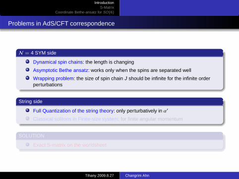
Problems in AdS/CFT correspondence
N = 4 SYM side
Dynamical spin chains: the length is changing
Asymptotic Bethe ansatz: works only when the spins are separated well
Wrapping problem: the size of spin chain J should be infinite for the infinite orderperturbations
String side
Full Quantization of the string theory: only perturbatively in α′
Classical solitons in Finite-size system: for finite angular momentum
SOLUTION
Exact S-matrix on the worldsheet
Tihany 2009.8.27 Changrim Ahn

IntroductionS-Matrix
Coordinate Bethe-ansatz for SO(6)
Problems in AdS/CFT correspondence
N = 4 SYM side
Dynamical spin chains: the length is changing
Asymptotic Bethe ansatz: works only when the spins are separated well
Wrapping problem: the size of spin chain J should be infinite for the infinite orderperturbations
String side
Full Quantization of the string theory: only perturbatively in α′
Classical solitons in Finite-size system: for finite angular momentum
SOLUTION
Exact S-matrix on the worldsheet
Tihany 2009.8.27 Changrim Ahn

IntroductionS-Matrix
Coordinate Bethe-ansatz for SO(6)
Yang-Baxter Equation
Due to the infinite # of conserved charges: momenta are preserved
Multiparticle scatterings are factorized into products of two-body S-matrices
S(p1,p2, . . . , pN) =N∏
i≤j
Sij(pi , pj)
Consistency in the order of factorization: YBE
S12S13S23 = S23S13S12, S12 = S ⊗ 1,S23 = 1 ⊗ S, . . .
=
1 2
3
1
2
3
YBE usually determines the matrix structure of S-matrix (ex) sine-Gordon model:BUT NOT HERE!
Tihany 2009.8.27 Changrim Ahn

IntroductionS-Matrix
Coordinate Bethe-ansatz for SO(6)
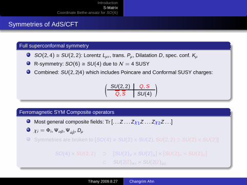
Symmetries of AdS/CFT
Full superconformal symmetry
SO(2, 4) � SU(2, 2): Lorentz Lµν, trans. Pµ, Dilatation D , spec. conf. Kµ
R-symmetry: SO(6) � SU(4) due to N = 4 SUSY
Combined: SU(2,2|4) which includes Poincare and Conformal SUSY charges:
(SU(2,2) Q,S
Q,S SU(4)
)
Ferromagnetic SYM Composite operators
Most general composite fields: Tr [. . .Z . . .Zχ1Z . . .Zχ2Z . . .]
χi = Φi ,Ψαβ,Ψαβ,Dµ
Symmetries are broken to [SO(4) � SU(2) × SU(2),SU(2,2) ⊃ SU(2) × SU(2)]
SO(4) × SU(2,2) ⊃ [SU(2)a × SU(2)a ] × [SU(2)α × SU(2)α]
⊂ SU(2|2)aα × SU(2|2)aα
Tihany 2009.8.27 Changrim Ahn

IntroductionS-Matrix
Coordinate Bethe-ansatz for SO(6)
Symmetries of AdS/CFT
Full superconformal symmetry
SO(2, 4) � SU(2, 2): Lorentz Lµν, trans. Pµ, Dilatation D , spec. conf. Kµ
R-symmetry: SO(6) � SU(4) due to N = 4 SUSY
Combined: SU(2,2|4) which includes Poincare and Conformal SUSY charges:
(SU(2,2) Q,S
Q,S SU(4)
)
Ferromagnetic SYM Composite operators
Most general composite fields: Tr [. . .Z . . .Zχ1Z . . .Zχ2Z . . .]
χi = Φi ,Ψαβ,Ψαβ,Dµ
Symmetries are broken to [SO(4) � SU(2) × SU(2),SU(2,2) ⊃ SU(2) × SU(2)]
SO(4) × SU(2,2) ⊃ [SU(2)a × SU(2)a ] × [SU(2)α × SU(2)α]
⊂ SU(2|2)aα × SU(2|2)aα
Tihany 2009.8.27 Changrim Ahn

IntroductionS-Matrix
Coordinate Bethe-ansatz for SO(6)
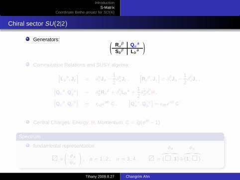
Chiral sector SU(2|2)
Generators: (Rα
β Qαa
Sbβ Lb
a
)
Commutation Relations and SUSY algebra:
[La
b , Jc
]= δb
c Ja −12δb
a Jc ,[Rα
β,Jγ]= δ
βγJα −
12δβαJγ ,
{Qα
a ,Q†bβ}
= δab Rα
β + δβαLb
a +12δa
bδβαH ,
{Qα
a ,Qβb}
= ǫαβǫab C ,
{Q†a
α,Q†bβ}= ǫab ǫ
αβ C†
Central Charges: Energy: H, Momentum: C = ig(eiP − 1)
Spectrum
fundamental representation
≡
(φaψα
), a = 1 , 2 , α = 3 , 4 . =
φa︷ ︸︸ ︷( , 1)⊕
ψα︷ ︸︸ ︷(1, ) .
Tihany 2009.8.27 Changrim Ahn
IntroductionS-Matrix
Coordinate Bethe-ansatz for SO(6)
Chiral sector SU(2|2)
Generators: (Rα
β Qαa
Sbβ Lb
a
)
Commutation Relations and SUSY algebra:
[La
b , Jc
]= δb
c Ja −12δb
a Jc ,[Rα
β,Jγ]= δ
βγJα −
12δβαJγ ,
{Qα
a ,Q†bβ}
= δab Rα
β + δβαLb
a +12δa
bδβαH ,
{Qα
a ,Qβb}
= ǫαβǫab C ,
{Q†a
α,Q†bβ}= ǫab ǫ
αβ C†
Central Charges: Energy: H, Momentum: C = ig(eiP − 1)
Spectrum
fundamental representation
≡
(φaψα
), a = 1 , 2 , α = 3 , 4 . =
φa︷ ︸︸ ︷( , 1)⊕
ψα︷ ︸︸ ︷(1, ) .
Tihany 2009.8.27 Changrim Ahn

IntroductionS-Matrix
Coordinate Bethe-ansatz for SO(6)
Full sector SU(2|2) × SU(2|2)
Fields Contents
Φi ≡ (φa ; φa) , Dµ ≡ (ψα;ψα) , Ψαβ ≡ (φa ;ψα) , Ψαβ ≡ (ψα; φa)
Tensor Product:
(;
)=
(, 1; , 1
)⊕
(, 1; 1,
)⊕
(1, ; ,1
)⊕
(1, ; 1,
)
Fields SU(2)S5 ,L × SU(2)AdS5 ,R × SU(2)S5 ,R × SU(2)AdS5 ,L
Z ( 1 , 1 ; 1 , 1 )Z ( 1 , 1 ; 1 , 1 )
Φi ( , 1 ; , 1 )
Dµ ( 1 , ; 1 , )Ψαβ ( , 1 ; 1 , )
Ψαβ ( 1 , ; , 1 )
Tihany 2009.8.27 Changrim Ahn

IntroductionS-Matrix
Coordinate Bethe-ansatz for SO(6)
Zamolodchikov-Faddeev algebra Approach
One particle state: |ei 〉 = |φa ;ψα〉 = A†i |0〉
Multi-particle state:
|ei1(p1)ei2 (p2) . . . ein (pn)〉in = A†i1(p1)A†
i2(p2) . . .A
†
in(pn)|0〉, p1 > p2 > . . . > pn
S-matrix: S · |ei(p1)ej(p2)〉in = Sklij (p1, p2)|el(p2)ek (p1)〉out
ZF algebra: A†i (p1)A†
j (p2) = Sklij (p1, p2)A
†
l (p2)A†
k (p1)
Tihany 2009.8.27 Changrim Ahn

IntroductionS-Matrix
Coordinate Bethe-ansatz for SO(6)
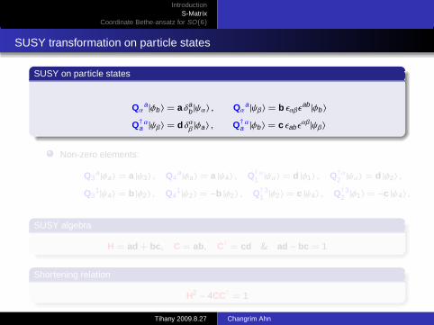
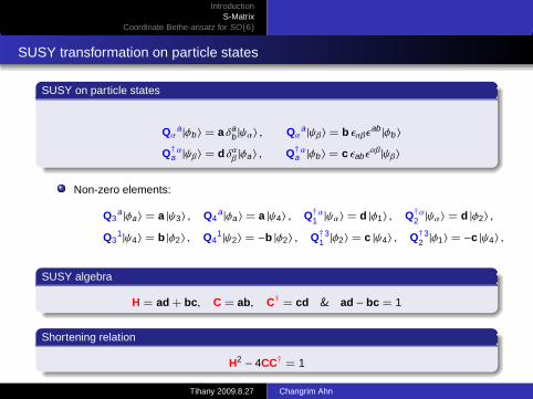
SUSY transformation on particle states
SUSY on particle states
Qαa |φb 〉 = a δa
b |ψα〉 , Qαa |ψβ〉 = b ǫαβǫab |φb 〉
Q†aα|ψβ〉 = d δαβ |φa〉 , Q†a
α |φb 〉 = c ǫabǫαβ|ψβ〉
Non-zero elements:
Q3a |φa〉 = a |ψ3〉 , Q4
a |φa 〉 = a |ψ4〉 , Q†1α |ψα〉 = d |φ1〉 , Q†2
α|ψα〉 = d |φ2〉 ,
Q31|ψ4〉 = b |φ2〉 , Q4
1 |ψ2〉 = −b |φ2〉 , Q†13|φ2〉 = c |ψ4〉 , Q†2
3|φ1〉 = −c |ψ4〉 ,
SUSY algebra
H = ad + bc, C = ab, C† = cd & ad − bc = 1
Shortening relation
H2 − 4CC† = 1
Tihany 2009.8.27 Changrim Ahn

IntroductionS-Matrix
Coordinate Bethe-ansatz for SO(6)
SUSY transformation on particle states
SUSY on particle states
Qαa |φb 〉 = a δa
b |ψα〉 , Qαa |ψβ〉 = b ǫαβǫab |φb 〉
Q†aα|ψβ〉 = d δαβ |φa〉 , Q†a
α |φb 〉 = c ǫabǫαβ|ψβ〉
Non-zero elements:
Q3a |φa〉 = a |ψ3〉 , Q4
a |φa 〉 = a |ψ4〉 , Q†1α |ψα〉 = d |φ1〉 , Q†2
α|ψα〉 = d |φ2〉 ,
Q31|ψ4〉 = b |φ2〉 , Q4
1 |ψ2〉 = −b |φ2〉 , Q†13|φ2〉 = c |ψ4〉 , Q†2
3|φ1〉 = −c |ψ4〉 ,
SUSY algebra
H = ad + bc, C = ab, C† = cd & ad − bc = 1
Shortening relation
H2 − 4CC† = 1
Tihany 2009.8.27 Changrim Ahn

IntroductionS-Matrix
Coordinate Bethe-ansatz for SO(6)
Unitary Representation
Unitary Representation:
a = ηeiξ, b = −ηe−ip/2
x−eiξ , c = −η
e−iξ
x+, d = ηe−ip/2e−iξ
spectral parameters:
η = eip/4√
ig(x− − x+)
x+ +1
x+− x− −
1x−
=ig
&x+
x−≡ eip
→ x± =e±ip/2
4g sin p2
1 +
√1 + 16g2 sin2 p
2
Central charges:
H = 1 +2igx+−
2igx−
=
√1 + 16g2 sin2 p
2, C = ige2iξ
(x+
x−− 1
)
Tihany 2009.8.27 Changrim Ahn

IntroductionS-Matrix
Coordinate Bethe-ansatz for SO(6)
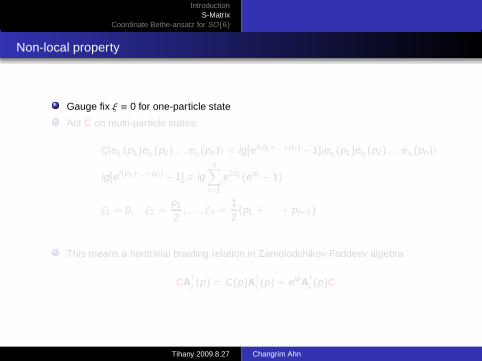
Non-local property
Gauge fix ξ ≡ 0 for one-particle state
Act C on multi-particle states:
C|ei1(p1)ei2(p2) . . . ein(pn)〉 = ig[ei(p1+...+pn) − 1]|ei1(p1)ei2(p2) . . . ein (pn)〉
ig[ei(p1+...+pn) − 1] ≡ ign∑
i=1
e2iξi (eipi − 1)
ξ1 = 0, ξ2 =p1
2, . . . , ξn =
12(p1 + . . .+ pn−1)
This means a nontrivial braiding relation in Zamolodchikov-Faddeev algebra
CA†i (p) = C(p)A†i (p) + eipA†i (p)C
Tihany 2009.8.27 Changrim Ahn
IntroductionS-Matrix
Coordinate Bethe-ansatz for SO(6)
Non-local property
Gauge fix ξ ≡ 0 for one-particle state
Act C on multi-particle states:
C|ei1(p1)ei2(p2) . . . ein(pn)〉 = ig[ei(p1+...+pn) − 1]|ei1(p1)ei2(p2) . . . ein (pn)〉
ig[ei(p1+...+pn) − 1] ≡ ign∑
i=1
e2iξi (eipi − 1)
ξ1 = 0, ξ2 =p1
2, . . . , ξn =
12(p1 + . . .+ pn−1)
This means a nontrivial braiding relation in Zamolodchikov-Faddeev algebra
CA†i (p) = C(p)A†i (p) + eipA†i (p)C
Tihany 2009.8.27 Changrim Ahn

IntroductionS-Matrix
Coordinate Bethe-ansatz for SO(6)
Zamolodchikov-Faddeev algebra
Commutation Relations with SU(2|2) generators
From SUSY transformation:
Lab A†(p) = A†(p) Lb
a + A†(p) Lab , Rα
βA†(p) = A†(p) Rβα + A†(p) Rα
β ,
Qαa A†(p) = A†(p) Qa
α (p) eiP/2 + A†(p)Σ Qαa ,
Q†aαA†(p) = A†(p) Q
α
a(p) e−iP/2 + A†(p)Σ Q†aα
Commutativity with SU(2|2) determines the S-matrix
[Qaα,S] =
[Q†a
α,S]=
[La
b ,S]=
[Rα
β,S]= 0
Tihany 2009.8.27 Changrim Ahn

IntroductionS-Matrix
Coordinate Bethe-ansatz for SO(6)
S-matrix elements
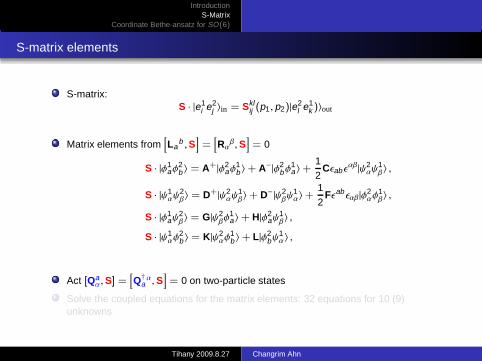
S-matrix:S · |e1
i e2j 〉in = Skl
ij (p1, p2)|e2l e1
k )〉out
Matrix elements from[La
b ,S]=
[Rα
β,S]= 0
S · |φ1aφ
2b 〉 = A+|φ2
aφ1b 〉+ A−|φ2
bφ1a〉+
12
Cǫabǫαβ|ψ2
αψ1β〉 ,
S · |ψ1αψ
2β〉 = D+|ψ2
αψ1β〉+ D−|ψ2
βψ1α〉+
12
Fǫabǫαβ|φ2αφ
1β〉 ,
S · |φ1aψ
2β〉 = G|ψ2
βφ1a〉+ H|φ2
aψ1β〉 ,
S · |ψ1αφ
2b 〉 = K|ψ2
αφ1b 〉+ L|φ2
bψ1α〉 ,
Act [Qaα,S] =
[Q†a
α,S]= 0 on two-particle states
Solve the coupled equations for the matrix elements: 32 equations for 10 (9)unknowns
Tihany 2009.8.27 Changrim Ahn

IntroductionS-Matrix
Coordinate Bethe-ansatz for SO(6)
S-matrix elements
S-matrix:S · |e1
i e2j 〉in = Skl
ij (p1, p2)|e2l e1
k )〉out
Matrix elements from[La
b ,S]=
[Rα
β,S]= 0
S · |φ1aφ
2b 〉 = A+|φ2
aφ1b 〉+ A−|φ2
bφ1a〉+
12
Cǫabǫαβ|ψ2
αψ1β〉 ,
S · |ψ1αψ
2β〉 = D+|ψ2
αψ1β〉+ D−|ψ2
βψ1α〉+
12
Fǫabǫαβ|φ2αφ
1β〉 ,
S · |φ1aψ
2β〉 = G|ψ2
βφ1a〉+ H|φ2
aψ1β〉 ,
S · |ψ1αφ
2b 〉 = K|ψ2
αφ1b 〉+ L|φ2
bψ1α〉 ,
Act [Qaα,S] =
[Q†a
α,S]= 0 on two-particle states
Solve the coupled equations for the matrix elements: 32 equations for 10 (9)unknowns
Tihany 2009.8.27 Changrim Ahn

IntroductionS-Matrix
Coordinate Bethe-ansatz for SO(6)
S-Matrix Structure
a1 0 0 0 | 0 0 0 0 | 0 0 0 0 | 0 00 a1+2 0 0 | −a2 0 0 0 | 0 0 0 −a7 | 0 00 0 a5 0 | 0 0 0 0 | a9 0 0 0 | 0 00 0 0 a5 | 0 0 0 0 | 0 0 0 0 | a9 0− − − − − − − − − − − − − − − − −
0 −a2 0 0 | a1+2 0 0 0 | 0 0 0 a7 | 0 00 0 0 0 | 0 a1 0 0 | 0 0 0 0 | 0 00 0 0 0 | 0 0 a5 0 | 0 a9 0 0 | 0 00 0 0 0 | 0 0 0 a5 | 0 0 0 0 | 0 a9
− − − − − − − − − − − − − − − − −
0 0 a10 0 | 0 0 0 0 | a6 0 0 0 | 0 00 0 0 0 | 0 0 a10 0 | 0 a6 0 0 | 0 00 0 0 0 | 0 0 0 0 | 0 0 a3 0 | 0 00 −a8 0 0 | a8 0 0 0 | 0 0 0 a3+4 | 0 0− − − − − − − − − − − − − − − − −
0 0 0 a10 | 0 0 0 0 | 0 0 0 0 | a6 00 0 0 0 | 0 0 0 a10 | 0 0 0 0 | 0 a6
0 a8 0 0 | −a8 0 0 0 | 0 0 0 −a4 | 0 00 0 0 0 | 0 0 0 0 | 0 0 0 0 | 0 0
Tihany 2009.8.27 Changrim Ahn
IntroductionS-Matrix
Coordinate Bethe-ansatz for SO(6)
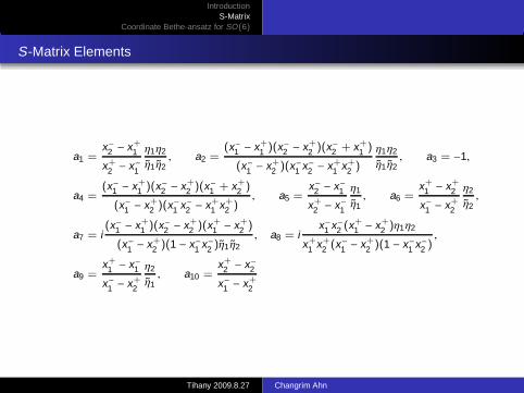
S-Matrix Elements
a1 =x−2 − x+
1
x+2 − x−1
η1η2
η1η2, a2 =
(x−1 − x+1 )(x−2 − x+
2 )(x−2 + x+1 )
(x−1 − x+2 )(x−1 x−2 − x+
1 x+2 )
η1η2
η1η2, a3 = −1,
a4 =(x−1 − x+
1 )(x−2 − x+2 )(x−1 + x+
2 )
(x−1 − x+2 )(x−1 x−2 − x+
1 x+2 )
, a5 =x−2 − x−1x+
2 − x−1
η1
η1, a6 =
x+1 − x+
2
x−1 − x+2
η2
η2,
a7 = i(x−1 − x+
1 )(x−2 − x+2 )(x+
1 − x+2 )
(x−1 − x+2 )(1 − x−1 x−2 )η1η2
, a8 = ix−1 x−2 (x+
1 − x+2 )η1η2
x+1 x+
2 (x−1 − x+2 )(1 − x−1 x−2 )
,
a9 =x+
1 − x−1x−1 − x+
2
η2
η1, a10 =
x+2 − x−2
x−1 − x+2
Tihany 2009.8.27 Changrim Ahn

IntroductionS-Matrix
Coordinate Bethe-ansatz for SO(6)
Charge conjugation
Torus parametrization
p = 2amz, sinp2
= sn(z, k ), H = dn(z, k ), k = −16g2
2ω1 = 4K(k ), 2ω2 = 4iK(1 − k ) − 4K(k )
x± =1g
( cnzsnz± i
)(1 + dnz)
Charge conjugation
E → −E, p → −p; x+ →1
x+, x− →
1x−
; z → z + ω2
Anti-particle operator
B†i (p) ≡ CijAj(−p), C =
(σ2 00 iσ2
)
Zamolodchikov-Faddeev algebra for anti-particles
A†i (p1)Aj(p2) = Aj′(p2)Sji′
j′ i(p2, p1)A†
i′(p1) + δ(p1,p2)δji
B†i (p1)Aj(p2) = Aj′(p2)S
ji′
j′ i(p2, p1)B†
i′(p1)
Tihany 2009.8.27 Changrim Ahn

IntroductionS-Matrix
Coordinate Bethe-ansatz for SO(6)
Charge conjugation
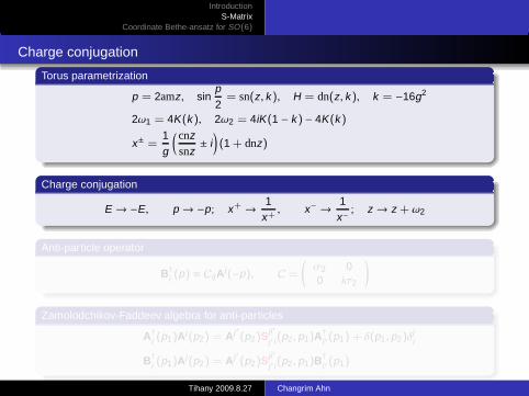
Torus parametrization
p = 2amz, sinp2
= sn(z, k ), H = dn(z, k ), k = −16g2
2ω1 = 4K(k ), 2ω2 = 4iK(1 − k ) − 4K(k )
x± =1g
( cnzsnz± i
)(1 + dnz)
Charge conjugation
E → −E, p → −p; x+ →1
x+, x− →
1x−
; z → z + ω2
Anti-particle operator
B†i (p) ≡ CijAj(−p), C =
(σ2 00 iσ2
)
Zamolodchikov-Faddeev algebra for anti-particles
A†i (p1)Aj(p2) = Aj′(p2)Sji′
j′ i(p2, p1)A†
i′(p1) + δ(p1,p2)δji
B†i (p1)Aj(p2) = Aj′(p2)S
ji′
j′ i(p2, p1)B†
i′(p1)
Tihany 2009.8.27 Changrim Ahn
IntroductionS-Matrix
Coordinate Bethe-ansatz for SO(6)
Charge conjugation
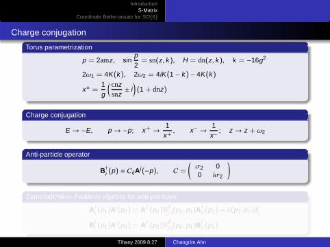
Torus parametrization
p = 2amz, sinp2
= sn(z, k ), H = dn(z, k ), k = −16g2
2ω1 = 4K(k ), 2ω2 = 4iK(1 − k ) − 4K(k )
x± =1g
( cnzsnz± i
)(1 + dnz)
Charge conjugation
E → −E, p → −p; x+ →1
x+, x− →
1x−
; z → z + ω2
Anti-particle operator
B†i (p) ≡ CijAj(−p), C =
(σ2 00 iσ2
)
Zamolodchikov-Faddeev algebra for anti-particles
A†i (p1)Aj(p2) = Aj′(p2)Sji′
j′ i(p2, p1)A†
i′(p1) + δ(p1,p2)δji
B†i (p1)Aj(p2) = Aj′(p2)S
ji′
j′ i(p2, p1)B†
i′(p1)
Tihany 2009.8.27 Changrim Ahn

IntroductionS-Matrix
Coordinate Bethe-ansatz for SO(6)
Charge conjugation
Torus parametrization
p = 2amz, sinp2
= sn(z, k ), H = dn(z, k ), k = −16g2
2ω1 = 4K(k ), 2ω2 = 4iK(1 − k ) − 4K(k )
x± =1g
( cnzsnz± i
)(1 + dnz)
Charge conjugation
E → −E, p → −p; x+ →1
x+, x− →
1x−
; z → z + ω2
Anti-particle operator
B†i (p) ≡ CijAj(−p), C =
(σ2 00 iσ2
)
Zamolodchikov-Faddeev algebra for anti-particles
A†i (p1)Aj(p2) = Aj′(p2)Sji′
j′ i(p2, p1)A†
i′(p1) + δ(p1,p2)δji
B†i (p1)Aj(p2) = Aj′(p2)S
ji′
j′ i(p2, p1)B†
i′(p1)
Tihany 2009.8.27 Changrim Ahn
IntroductionS-Matrix
Coordinate Bethe-ansatz for SO(6)
Crossing relation
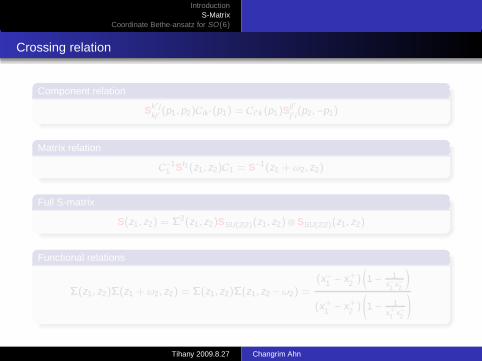
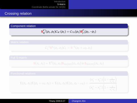
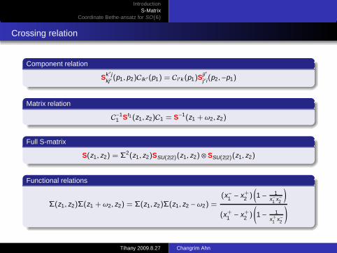
Component relation
Sk ′ jkj′ (p1, p2)Cik ′(p1) = Ci′k (p1)S
ji′
j′ i(p2,−p1)
Matrix relation
C−11 St1(z1, z2)C1 = S−1(z1 + ω2, z2)
Full S-matrix
S(z1, z2) = Σ2(z1, z2)SSU(2|2)(z1, z2) ⊗ SSU(2|2)(z1, z2)
Functional relations
Σ(z1, z2)Σ(z1 + ω2, z2) = Σ(z1, z2)Σ(z1, z2 − ω2) =(x−1 − x+
2 )(1 − 1
x−1 x−2
)
(x+1 − x+
2 )
(1 − 1
x+1 x−2
)
Tihany 2009.8.27 Changrim Ahn
IntroductionS-Matrix
Coordinate Bethe-ansatz for SO(6)
Crossing relation
Component relation
Sk ′ jkj′ (p1, p2)Cik ′(p1) = Ci′k (p1)S
ji′
j′ i(p2,−p1)
Matrix relation
C−11 St1(z1, z2)C1 = S−1(z1 + ω2, z2)
Full S-matrix
S(z1, z2) = Σ2(z1, z2)SSU(2|2)(z1, z2) ⊗ SSU(2|2)(z1, z2)
Functional relations
Σ(z1, z2)Σ(z1 + ω2, z2) = Σ(z1, z2)Σ(z1, z2 − ω2) =(x−1 − x+
2 )(1 − 1
x−1 x−2
)
(x+1 − x+
2 )
(1 − 1
x+1 x−2
)
Tihany 2009.8.27 Changrim Ahn

IntroductionS-Matrix
Coordinate Bethe-ansatz for SO(6)
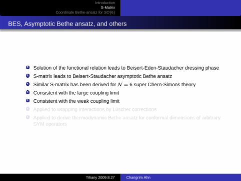
BES, Asymptotic Bethe ansatz, and others
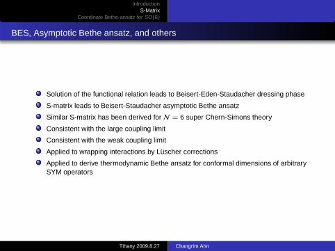
Solution of the functional relation leads to Beisert-Eden-Staudacher dressing phase
S-matrix leads to Beisert-Staudacher asymptotic Bethe ansatz
Similar S-matrix has been derived for N = 6 super Chern-Simons theory
Consistent with the large coupling limit
Consistent with the weak coupling limit
Applied to wrapping interactions by Luscher corrections
Applied to derive thermodynamic Bethe ansatz for conformal dimensions of arbitrarySYM operators
Tihany 2009.8.27 Changrim Ahn

IntroductionS-Matrix
Coordinate Bethe-ansatz for SO(6)
BES, Asymptotic Bethe ansatz, and others
Solution of the functional relation leads to Beisert-Eden-Staudacher dressing phase
S-matrix leads to Beisert-Staudacher asymptotic Bethe ansatz
Similar S-matrix has been derived for N = 6 super Chern-Simons theory
Consistent with the large coupling limit
Consistent with the weak coupling limit
Applied to wrapping interactions by Luscher corrections
Applied to derive thermodynamic Bethe ansatz for conformal dimensions of arbitrarySYM operators
Tihany 2009.8.27 Changrim Ahn

IntroductionS-Matrix
Coordinate Bethe-ansatz for SO(6)
Coordinate Bethe-ansatz
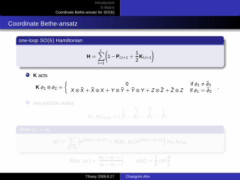
one-loop SO(6) Hamiltonian
H =L∑
l=1
(1 − Pl,l+1 +
12
Kl,l+1
)
K acts
K φ1 ⊗ φ2 =
{0 if φ1 , φ2
X ⊗ X + X ⊗ X + Y ⊗ Y + Y ⊗ Y + Z ⊗ Z + Z ⊗ Z if φ1 = φ2.
two-particle states
|x1, x2〉φ1φ2 = |
1↓
Z · · ·
x1↓
φ1 · · ·
x2↓
φ2 · · ·
L↓
Z〉
when φ1 = φ2
|ψ〉 =∑
x1<x2
[ei(p1x1+p2x2) + S(p2 ,p1) ei(p2x1+p1x2)
]|x1, x2〉φφ
S(p2 , p1) =u2 − u1 + iu2 − u1 − i
, u(p) =12
cotp2
Tihany 2009.8.27 Changrim Ahn

IntroductionS-Matrix
Coordinate Bethe-ansatz for SO(6)
Coordinate Bethe-ansatz
one-loop SO(6) Hamiltonian
H =L∑
l=1
(1 − Pl,l+1 +
12
Kl,l+1
)
K acts
K φ1 ⊗ φ2 =
{0 if φ1 , φ2
X ⊗ X + X ⊗ X + Y ⊗ Y + Y ⊗ Y + Z ⊗ Z + Z ⊗ Z if φ1 = φ2.
two-particle states
|x1, x2〉φ1φ2 = |
1↓
Z · · ·
x1↓
φ1 · · ·
x2↓
φ2 · · ·
L↓
Z〉
when φ1 = φ2
|ψ〉 =∑
x1<x2
[ei(p1x1+p2x2) + S(p2 ,p1) ei(p2x1+p1x2)
]|x1, x2〉φφ
S(p2 , p1) =u2 − u1 + iu2 − u1 − i
, u(p) =12
cotp2
Tihany 2009.8.27 Changrim Ahn

IntroductionS-Matrix
Coordinate Bethe-ansatz for SO(6)
Coordinate Bethe-ansatz
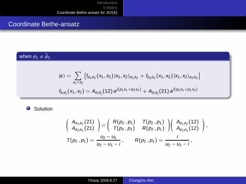
when φ1 , φ2
|ψ〉 =∑
x1<x2
{fφ1φ2(x1, x2) |x1, x2〉φ1φ2 + fφ2φ1(x1, x2) |x1, x2〉φ2φ1
}
fφiφj (x1, x2) = Aφiφj (12) ei(p1x1+p2x2) + Aφiφj (21) ei(p2x1+p1x2)
Solution
(Aφ1φ2 (21)Aφ2φ1 (21)
)=
(R(p2 , p1) T(p2 ,p1)T(p2 , p1) R(p2 , p1)
) (Aφ1φ2(12)Aφ2φ1(12)
),
T(p2 , p1) =u2 − u1
u2 − u1 − i, R(p2 , p1) =
iu2 − u1 − i
,
Tihany 2009.8.27 Changrim Ahn

IntroductionS-Matrix
Coordinate Bethe-ansatz for SO(6)
Coordinate Bethe-ansatz
when φ1 , φ2
|ψ〉 =∑
x1<x2
{fφ1φ2(x1, x2) |x1, x2〉φ1φ2 + fφ2φ1(x1, x2) |x1, x2〉φ2φ1
}
fφiφj (x1, x2) = Aφiφj (12) ei(p1x1+p2x2) + Aφiφj (21) ei(p2x1+p1x2)
Solution
(Aφ1φ2 (21)Aφ2φ1 (21)
)=
(R(p2 , p1) T(p2 ,p1)T(p2 , p1) R(p2 , p1)
) (Aφ1φ2(12)Aφ2φ1(12)
),
T(p2 , p1) =u2 − u1
u2 − u1 − i, R(p2 , p1) =
iu2 − u1 − i
,
Tihany 2009.8.27 Changrim Ahn

IntroductionS-Matrix
Coordinate Bethe-ansatz for SO(6)
Coordinate Bethe-ansatz
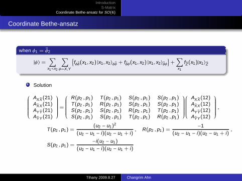
when φ1 = φ2
|ψ〉 =∑
x1<x2
∑
φ=X ,Y
{fφφ(x1, x2) |x1, x2〉φφ + fφφ(x1, x2) |x1, x2〉φφ
}+
∑
x1
fZ(x1)|x1〉Z
Solution
AXX (21)AXX (21)AYY (21)AYY (21)
=
R(p2 , p1) T(p2 , p1) S(p2 , p1) S(p2 , p1)T(p2 ,p1) R(p2 ,p1) S(p2 , p1) S(p2 , p1)S(p2 , p1) S(p2 , p1) R(p2 , p1) T(p2 , p1)S(p2 , p1) S(p2 , p1) T(p2 ,p1) R(p2 ,p1)
AXX (12)AXX (12)AYY (12)AYY (12)
,
T(p2 , p1) =(u2 − u1)
2
(u2 − u1 − i)(u2 − u1 + i), R(p2 ,p1) =
−1(u2 − u1 − i)(u2 − u1 + i)
,
S(p2 , p1) =−i(u2 − u1)
(u2 − u1 − i)(u2 − u1 + i)
Tihany 2009.8.27 Changrim Ahn

IntroductionS-Matrix
Coordinate Bethe-ansatz for SO(6)
Coordinate Bethe-ansatz
when φ1 = φ2
|ψ〉 =∑
x1<x2
∑
φ=X ,Y
{fφφ(x1, x2) |x1, x2〉φφ + fφφ(x1, x2) |x1, x2〉φφ
}+
∑
x1
fZ(x1)|x1〉Z
Solution
AXX (21)AXX (21)AYY (21)AYY (21)
=
R(p2 , p1) T(p2 , p1) S(p2 , p1) S(p2 , p1)T(p2 ,p1) R(p2 ,p1) S(p2 , p1) S(p2 , p1)S(p2 , p1) S(p2 , p1) R(p2 , p1) T(p2 , p1)S(p2 , p1) S(p2 , p1) T(p2 ,p1) R(p2 ,p1)
AXX (12)AXX (12)AYY (12)AYY (12)
,
T(p2 , p1) =(u2 − u1)
2
(u2 − u1 − i)(u2 − u1 + i), R(p2 ,p1) =
−1(u2 − u1 − i)(u2 − u1 + i)
,
S(p2 , p1) =−i(u2 − u1)
(u2 − u1 − i)(u2 − u1 + i)
Tihany 2009.8.27 Changrim Ahn

IntroductionS-Matrix
Coordinate Bethe-ansatz for SO(6)
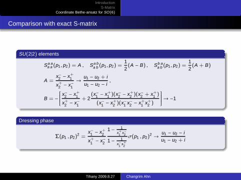
Comparison with exact S-matrix
SU(2|2) elements
Sa aa a (p1,p2) = A , Sa b
a b (p1,p2) =12(A − B) , Sb a
a b (p1, p2) =12(A + B)
A =x−2 − x+
1
x+2 − x−1
→u1 − u2 + iu1 − u2 − i
,
B = −
x−2 − x+
1
x+2 − x−1
+ 2(x−1 − x+
1 )(x−2 − x+2 )(x−2 + x+
1 )
(x−1 − x+2 )(x−1 x−2 − x+
1 x+2 )
→ −1
Dressing phase
Σ(p1 , p2)2 =
x−1 − x+2
x+1 − x−2
1 − 1x+
1 x−2
1 − 1x−1 x+
2
σ(p1 , p2)2 →
u1 − u2 − iu1 − u2 + i
Tihany 2009.8.27 Changrim Ahn

IntroductionS-Matrix
Coordinate Bethe-ansatz for SO(6)
Comparison with exact S-matrix
SU(2|2) elements
Sa aa a (p1,p2) = A , Sa b
a b (p1,p2) =12(A − B) , Sb a
a b (p1, p2) =12(A + B)
A =x−2 − x+
1
x+2 − x−1
→u1 − u2 + iu1 − u2 − i
,
B = −
x−2 − x+
1
x+2 − x−1
+ 2(x−1 − x+
1 )(x−2 − x+2 )(x−2 + x+
1 )
(x−1 − x+2 )(x−1 x−2 − x+
1 x+2 )
→ −1
Dressing phase
Σ(p1 , p2)2 =
x−1 − x+2
x+1 − x−2
1 − 1x+
1 x−2
1 − 1x−1 x+
2
σ(p1 , p2)2 →
u1 − u2 − iu1 − u2 + i
Tihany 2009.8.27 Changrim Ahn

IntroductionS-Matrix
Coordinate Bethe-ansatz for SO(6)
Comparison with exact S-matrix
The same type:
S(p1,p2) ≡(Σ(p1, p2) Sa a
a a (p1, p2))2
= S20 A2 →
u1 − u2 + iu1 − u2 − i
φ1 , φ2 type:
T(p1, p2) =12
S20 A(A−B)→
u1 − u2
u1 − u2 − i, R(p1, p2) =
12
S20 A(A+B)→
iu1 − u2 − i
φ1 = φ2 type:
T(p1, p2) =14
S20 (A − B)2 →
(u1 − u2)2
(u1 − u2 − i)(u1 − u2 + i),
R(p1, p2) =14
S20 (A + B)2 →
−1(u1 − u2 − i)(u1 − u2 + i)
,
S(p1, p2) =14
S20 (A − B)(A + B)→
i(u1 − u2)
(u1 − u2 − i)(u1 − u2 + i),
Tihany 2009.8.27 Changrim Ahn