Embed Size (px)
Citation preview

Evolutionary Search on Fitness Landscapes
with Neutral Networks
Lionel Barnett
Submitted for the degree of D. Phil.
University of Sussex
August, 2003

Declaration
I hereby declare that this thesis has not been submitted, either in the same or different form, to this
or any other university for a degree.
Signature:

Acknowledgements
Cuando me buscas, no estoyCuando me encuentras, no soy yo
Manu Chao –El Desaparecido
To Inman, for the awkward questions.
To Txaro and Asier, for their support and impatience.

Evolutionary Search on Fitness Landscapes
with Neutral Networks
Lionel Barnett
Summary
In the field of search and optimisation every theorist and practitioner should be aware of the so-calledNo Free Lunch Theorems(Wolpert & Macready, 1997) which imply that given any opti-misation algorithm, should that algorithm perform better than random search on some class ofproblems, then there is guaranteed to exist another class of problems for which the same algo-rithm performsworsethan random search. Thus we can say for certain that there is no such thingas an effective “general purpose” search algorithm. The obverse is thatthe more we know abouta class of problems, the better equipped we are to design effective optimisation algorithms forthat class. This thesis addresses a quite specific class of optimisation problems - and optimisationalgorithms. Our approach is to analyse statistical characteristics of the problem search space andthence to identify the algorithms (within the class considered) whichexploit these characteristics- we pay for our lunch, one might say.
The class of optimisation problems addressed might loosely be described ascorrelated fitnesslandscapes with large-scale neutrality; the class of search algorithms asevolutionary search pro-cesses. Why we might wish to study these problems and processes is discussed in detail in theIntroduction. A brief answer is that problems of this type arise in some novel engineering tasks.What they have in common is huge search spaces and inscrutable complexity arising from a richand complex interaction of the designed artifact with the “real world” - the messy world, that is,outside our computers. The huge search spaces and intractable structures - and hence lack of obvi-ous design heuristics - suggests astochasticapproach; but “traditional” stochastic techniques suchas Genetic Algorithms have frequently been designed with rather different search spaces in mind.This thesis examines how evolutionary search techniques might need to be be re-considered forthis type of problem.
Submitted for the degree of D. Phil.
University of Sussex
August, 2003

Contents
1 Introduction 1
1.1 Evolutionary Search. . . . . . . . . . . . . . . . . . . . . . . . . . . . . . . . . 2
1.1.1 The Fitness Landscaper - An Anecdotal Example. . . . . . . . . . . . . 4
1.1.2 Model Landscapes. . . . . . . . . . . . . . . . . . . . . . . . . . . . . 5
1.1.3 Landscape Statistics. . . . . . . . . . . . . . . . . . . . . . . . . . . . 6
1.2 Why Neutrality?. . . . . . . . . . . . . . . . . . . . . . . . . . . . . . . . . . . 7
1.3 Overview . . . . . . . . . . . . . . . . . . . . . . . . . . . . . . . . . . . . . . 8
1.3.1 Organisation . . . . . . . . . . . . . . . . . . . . . . . . . . . . . . . . 8
1.3.2 Summary of Conclusions. . . . . . . . . . . . . . . . . . . . . . . . . . 10
2 Fitness Landscapes 11
2.1 Definitions. . . . . . . . . . . . . . . . . . . . . . . . . . . . . . . . . . . . . . 12
2.1.1 Neutral Partitionings and Neutral Networks. . . . . . . . . . . . . . . . 12
2.2 Fitness-Independent Structure. . . . . . . . . . . . . . . . . . . . . . . . . . . 13
2.2.1 Mutation Modes and Mutation Operators. . . . . . . . . . . . . . . . . 13
2.2.2 The Mutation Matrix. . . . . . . . . . . . . . . . . . . . . . . . . . . . 16
2.2.3 Subspace Entropy and Markov Partitionings. . . . . . . . . . . . . . . . 17
2.2.4 Multiplicative Mutation Approximations. . . . . . . . . . . . . . . . . 19
2.2.5 Optimal Mutation. . . . . . . . . . . . . . . . . . . . . . . . . . . . . . 22
2.2.6 Innovations, Accessibility and Percolation of Neutral Networks. . . . . 23
2.3 Fitness-Dependent Structure. . . . . . . . . . . . . . . . . . . . . . . . . . . . 28
2.3.1 The Mutant Fitness Distribution. . . . . . . . . . . . . . . . . . . . . . 28
2.3.2 Parent-Mutant Fitness Correlation. . . . . . . . . . . . . . . . . . . . . 29
2.3.3 Linear Correlation. . . . . . . . . . . . . . . . . . . . . . . . . . . . . 30
2.3.4 Evolvability. . . . . . . . . . . . . . . . . . . . . . . . . . . . . . . . . 31
2.4 Random Fitness Landscapes. . . . . . . . . . . . . . . . . . . . . . . . . . . . 34
3 Evolutionary Dynamics 38
3.1 Populations. . . . . . . . . . . . . . . . . . . . . . . . . . . . . . . . . . . . . 38
3.2 Selection Operators and Evolutionary Operators. . . . . . . . . . . . . . . . . . 39
3.2.1 Evolutionary Operators. . . . . . . . . . . . . . . . . . . . . . . . . . . 40
3.2.2 Evolutionary Processes. . . . . . . . . . . . . . . . . . . . . . . . . . . 44
3.3 Statistical Dynamics . . . . . . . . . . . . . . . . . . . . . . . . . . . . . . . . 45
3.3.1 Coarse-graining and the Maximum Entropy Approximation. . . . . . . 46
3.4 Epochal Dynamics. . . . . . . . . . . . . . . . . . . . . . . . . . . . . . . . . 48
3.4.1 Analysing Epochal Dynamics - Fitness Barriers and Entropy Barriers. . 50
3.5 Measuring Search Efficiency. . . . . . . . . . . . . . . . . . . . . . . . . . . . 51

Contents vi
4 The Utility of Neutral Drift 55
4.1 The Nervous Ant . . . . . . . . . . . . . . . . . . . . . . . . . . . . . . . . . . 58
4.1.1 The independent mutant approximation. . . . . . . . . . . . . . . . . . 67
4.2 Neutral Drift in Populations. . . . . . . . . . . . . . . . . . . . . . . . . . . . . 69
5 ε-Correlated Landscapes 70
5.1 Introduction. . . . . . . . . . . . . . . . . . . . . . . . . . . . . . . . . . . . . 70
5.2 Optimal Mutation Rate. . . . . . . . . . . . . . . . . . . . . . . . . . . . . . . 72
5.3 Optimal Evolutionary Search. . . . . . . . . . . . . . . . . . . . . . . . . . . . 73
5.3.1 Adaptive netcrawling and the 1/eNeutral Mutation Rule. . . . . . . . . 75
5.3.2 Random search onε-correlated fitness landscapes. . . . . . . . . . . . . 76
5.3.3 The netcrawler onε-correlated fitness landscapes. . . . . . . . . . . . . 77
5.4 Royal Road Fitness Landscapes. . . . . . . . . . . . . . . . . . . . . . . . . . 78
5.4.1 Definitions and statistics. . . . . . . . . . . . . . . . . . . . . . . . . . 78
5.4.2 Search performance on Royal Road landscapes. . . . . . . . . . . . . . 88
5.5 Discussion. . . . . . . . . . . . . . . . . . . . . . . . . . . . . . . . . . . . . .100
6 The NKp Family of Random Fitness Landscapes 103
6.1 Background. . . . . . . . . . . . . . . . . . . . . . . . . . . . . . . . . . . . .103
6.1.1 Construction . . . . . . . . . . . . . . . . . . . . . . . . . . . . . . . .104
6.2 Statistical Analysis - Global Structure. . . . . . . . . . . . . . . . . . . . . . . 107
6.2.1 NK landscapes - Correlation. . . . . . . . . . . . . . . . . . . . . . . . 107
6.2.2 NKp Landscapes - Contributing Features. . . . . . . . . . . . . . . . . 109
6.2.3 NKp Landscapes - Neutral and Lethal Mutation. . . . . . . . . . . . . . 110
6.3 Statistical Analysis - Fitness-Dependent Structure. . . . . . . . . . . . . . . . . 113
6.3.1 NK Landscapes - Mean Mutant Fitness. . . . . . . . . . . . . . . . . . 113
6.3.2 NKp Landscapes - Fitness-dependence of Neutral and Lethal Mutation. 115
6.3.3 NKp Landscapes - Mutant Distribution. . . . . . . . . . . . . . . . . . 116
6.4 Landscape Modelling with NKp Landscapes. . . . . . . . . . . . . . . . . . . . 125
6.4.1 Estimating landscape parameters. . . . . . . . . . . . . . . . . . . . . . 128
6.4.2 Notes on NKp computer implementation. . . . . . . . . . . . . . . . . 128
6.4.3 Neutral Network Statistics. . . . . . . . . . . . . . . . . . . . . . . . . 129
6.4.4 Hill-climbing on NKp Landscapes. . . . . . . . . . . . . . . . . . . . . 137
7 Recombination 141
7.1 The Building Block Hypothesis. . . . . . . . . . . . . . . . . . . . . . . . . . . 142
7.2 Genetic Drift and Hitch-hiking. . . . . . . . . . . . . . . . . . . . . . . . . . . 145
7.3 Recombination, Error Thresholds and the Bi-stability Barrier. . . . . . . . . . . 146
7.3.1 The Quasi-species Model. . . . . . . . . . . . . . . . . . . . . . . . . . 147
7.3.2 The Asexual quasi-species. . . . . . . . . . . . . . . . . . . . . . . . . 149
7.3.3 The Sexual quasi-species. . . . . . . . . . . . . . . . . . . . . . . . . . 151
7.3.4 Approximations for the Sexual quasi-species. . . . . . . . . . . . . . . 152
7.3.5 Stability of Equilibria. . . . . . . . . . . . . . . . . . . . . . . . . . . . 155

Contents vii
7.3.6 Discussion . . . . . . . . . . . . . . . . . . . . . . . . . . . . . . . . .159
8 Conclusion 162
8.1 Review of Results. . . . . . . . . . . . . . . . . . . . . . . . . . . . . . . . . .162
8.2 Directions for Further Research. . . . . . . . . . . . . . . . . . . . . . . . . . . 169
8.3 Closing Remarks. . . . . . . . . . . . . . . . . . . . . . . . . . . . . . . . . .171
References 172
A Evolutionary Operators 179
A.1 Definitions. . . . . . . . . . . . . . . . . . . . . . . . . . . . . . . . . . . . . .179
A.2 Examples . . . . . . . . . . . . . . . . . . . . . . . . . . . . . . . . . . . . . .184
A.3 “Lifting” the Selection Operator . . . . . . . . . . . . . . . . . . . . . . . . . . 185
B Transformations of the Quasi-species Generating Functions 187
B.1 Transformation ofg(z) by Mutation . . . . . . . . . . . . . . . . . . . . . . . . 187
B.2 Transformation ofg(z) by Recombination. . . . . . . . . . . . . . . . . . . . . 187

List of Figures
2.1 Expected (cumulative) innovations (Eq. (2.47)) plotted against time (logarithmic
scale) for a neutral network with access to three networks. Mutation probabilities
are 0.001, 0.1 and 0.899. . . . . . . . . . . . . . . . . . . . . . . . . . . . . . . 25
2.2 Mutant fitness distribution with “tail” of fitness-increasing mutants.. . . . . . . 32
3.1 Typical evolutionary dynamics on a fitness landscape featuring neutral networks.48
4.1 Independent mutantsX1,X2 of the uniform random sequenceX and independent
mutantsY1,Y2 of the independent uniform random sequencesY,Y′ respectively, on
a neutral networkΓ as in Prop.4.0.1. . . . . . . . . . . . . . . . . . . . . . . . . 57
4.2 The 4-sequence neutral network plus portal (for fixed 1-bit mutation) of Exam-
ple4.1.1on the cube0,13. Red nodes represent sequences onΓ, the green node
represents the (single) portal inΠ. . . . . . . . . . . . . . . . . . . . . . . . . . 61
4.3 Portal (non-)discovery probabilityP(T(q) > t) of Eq. (4.19), plotted against drift
parameterq for the Γ, Π of Example4.1.1with fixed 1-point mutation and off-
network-proportional initial placement probabilities, fort = 1,2, . . . ,8. Note that,
as regards discovery of portals, thesmallerthe probabilityP(T(q) > t) thebetter. 62
4.4 P(T(q) > t) plotted againstq as in Fig.4.4, except that here initial placement
probabilities are equal (“maximum entropy” condition).. . . . . . . . . . . . . . 63
5.1 The optimum constant mutation raten∗j = [u∗j ] of Prop.5.2.1plotted againstν j ,ν j+1 73
5.2 Royal Road percolation indicesP j for 1-point mutation, plotted forN = 16 and a
few values ofK. . . . . . . . . . . . . . . . . . . . . . . . . . . . . . . . . . . . 81
5.3 Royal Road evolvability drift factorsDevolj for 1-point mutation, plotted forN = 16
and few values ofK. . . . . . . . . . . . . . . . . . . . . . . . . . . . . . . . . 83
5.4 Portal discovery probability plotted against per-sequence mutation rate for a Royal
Road landscape with parametersN = 12, K = 4 and several values ofj = network
number, forn-point (constant) and per-locus (Poisson) mutation modes. Solid
lines give the analytic values from Eq. (5.4) and Eq. (5.5); the vertical arrows indi-
cate the optimum mutation rates of Prop.5.2.1. Points are values from a simulation
with a sample size ofS= 100,000. Error bars give 95% confidence limits.. . . . 85
5.5 Portal discovery probability plotted against per-sequence mutation rate for a Royal
Road landscape with parametersN = 12, K = 8 and several values ofj = network
number, forn-point (constant) and per-locus (Poisson) mutation modes. Solid
lines give the analytic values from Eq. (5.4) and Eq. (5.5); the vertical arrows indi-
cate the optimum mutation rates of Prop.5.2.1. Points are values from a simulation
with a sample size ofS= 1000,000. Error bars give 95% confidence limits.. . . 86

List of Figures ix
5.6 A typical run of an adaptive netcrawler (Section5.3.1) on a Royal Road fitness
landscape. The horizontal axis measures fitness evaluations. The current epoch
of the netcrawler (i.e. current neutral network) is plotted against the left-hand
vertical axis. Actual and optimal mutation rates (in bits) are plotted against the
right-hand vertical axis. Parameters are:N = 16, K = 12, “window” size= 100
fitness evaluations, initial/maximum mutation rate= 16 (= N). . . . . . . . . . 88
5.7 Sample estimates of expected first passage timesTi for an (optimal) netcrawler
on Royal Road landscapes for a range ofN andK values. Vertical axes measure
times in fitness evaluations, on a logarithmic scale. The horizontal axes specify the
epoch (i.e. the network numberi). Means (points) and standard deviations (error
bars) were estimated using Eq. (5.62) and Eq. (5.63); in all cases sample size
was 1000 and the netcrawlers were run for 1,000,000 fitness evaluations (which
proved sufficient to ensure thatp < 0.1). Solid lines plot the theoretical estimate
Eq. (5.20) for E(Ti) . . . . . . . . . . . . . . . . . . . . . . . . . . . . . . . . . 91
5.8 Optimised GA performance (no recombination) on a Royal Road landscape with
N = 8, K = 8: mean best-so-far fitness (sample size 1,000 runs) plotted against
time in fitness evaluations. See text and Table5.1 for key and parameters. The
bottom figure shows a histogram of mean best-so-far fitness at the end of each run,
ranked by performance.. . . . . . . . . . . . . . . . . . . . . . . . . . . . . . . 96
5.9 Optimised GA performance (with recombination) on a Royal Road landscape with
N = 8, K = 8: mean best-so-far fitness (sample size 1,000 runs) plotted against
time in fitness evaluations. See text and Table5.2 for key and parameters. The
bottom figure shows a histogram of mean best-so-far fitness at the end of each run,
ranked by performance.. . . . . . . . . . . . . . . . . . . . . . . . . . . . . . . 97
5.10 Recombination only: performance of a fitness-proportional GA with multinomial
sampling and power law scaling on a Royal Road landscape withN = 8, K = 8:
mean best-so-far fitness (sample size 1,000 runs) plotted against time in fitness
evaluations. In the top figure selection pressure is high (scale factor= 10) and
population size is varied. In the bottom figure population size is high (= 1,000)
and selection pressure is varied.. . . . . . . . . . . . . . . . . . . . . . . . . . 101
6.1 Fitness-dependent neutrality (top figure) and lethal mutation probability (bottom
figure) for NKp landscapes plotted againstd, w for a range ofw values. Param-
eters: variable epistasis, Gaussian underlying distribution with varianceσ2 = 1,
F = 20,N = 32,κ = 0.125,p = 0.99. . . . . . . . . . . . . . . . . . . . . . . . 117
6.2 Fitness-dependent neutral degree variancevar(∆ | W = w) plotted against a range
of w values and auto-correlationρ(1) = 1− κ. Parameters: variable epistasis,
Gaussian underlying distribution with varianceσ2 = 1,F = 20,N = 32,κ = 0.125,
p = 0.99. . . . . . . . . . . . . . . . . . . . . . . . . . . . . . . . . . . . . . .118

List of Figures x
6.3 The conditional probability density functionϕ(d)(w′|w) of the continuous part of
the NKp mutant distributionW(d)∣∣(W = w) of Eq. (6.74) at Hamming distance
d = 1 (top figure) andd = 2 (bottom figure), plotted againstw′ for several (posi-
tive) values ofw. Parameters: variable epistasis, Gaussian underlying distribution
with varianceσ2 = 1, F = 20,N = 32,κ = 0.125,p = 0.99. . . . . . . . . . . . 121
6.4 The NKp evolvability statisticE (d |w) of Eq. (6.76) and Eq. (6.79) plotted against
d and 0≤ w ≤ 1 (top figure) and 0≤ w ≤ 0.01 (bottom figure). Parameters:
variable epistasis, Gaussian underlying distribution with varianceσ2 = 1, F = 20,
N = 32,κ = 0.125,p = 0.99. . . . . . . . . . . . . . . . . . . . . . . . . . . . . 123
6.5 Optimum mutation rates calculated from the evolvability statistic (Eq.6.76) and
estimated optimum rates based on neutrality (Eq.6.61) and the 1/eNeutral Muta-
tion Rule (see text) for constant (top figure) and Poisson (bottom figure) mutation
modes. Parameters: variable epistasis, Gaussian underlying distribution with vari-
anceσ2 = 1, F = 20,N = 32,κ = 0.125,p = 0.99. . . . . . . . . . . . . . . . . 126
6.6 Exhaustively sampled NKp mean neutral network size for short sequence length
baseline parameters (variable epistasis, Gaussian underlying distribution with vari-
anceσ2 = 1,F = 20,N = 16,κ = 0.375,p= 0.99) plotted against fitness. Number
of landscapes sampled= 10,000. Error bars indicate 1 standard deviation (note
large variance). The dashed line is the analytic (estimated) valueE(S | W = w)of Eq. (6.81) and (6.82). . . . . . . . . . . . . . . . . . . . . . . . . . . . . . . 131
6.7 Fitness-dependence of (estimated) mean neutral network sizeE(S | W = w) (note
log scale) for NKp landscapes plotted against neutrality (top figure) and epistasis
(bottom figure) for a range ofw values. Parameters: variable epistasis, Gaussian
underlying distribution with varianceσ2 = 1, F = 20, N = 32, κ = 0.125 (top
figure),p = 0.99 (bottom figure).. . . . . . . . . . . . . . . . . . . . . . . . . . 132
6.8 Exhaustively sampled NKp mean number of networks (binned vs. fitness) for
short sequence length baseline parameters (variable epistasis, Gaussian underlying
distribution with varianceσ2 = 1, F = 20,N = 16,κ = 0.375,p= 0.99). Number
of landscapes sampled= 1000, error bars indicate 1 standard deviation. Mean
total number of networks per landscape was≈ 78.3±44.1. . . . . . . . . . . . . 133
6.9 Top: Mean (sampled) effective accessible networks (percolation index) for con-
stant 1-bit mutation plotted against network fitness. Error bars denote one standard
deviation.Bottom:Cumulative innovations plotted against neutral walk steps. In-
set shows first 100 steps of walk. Parameters: variable epistasis, Gaussian under-
lying distribution with varianceσ2 = 1, F = 40, N = 64, κ = 0.1875,p = 0.999.
Sample size = 1,000 landscapes, neutral walk steps = 10,000. . . . . . . . . . . 135
6.10 Top: Mean (sampled) effective accessible networks (percolation index) for con-
stant 4-bit mutation plotted against network fitness. Error bars denote one standard
deviation.Bottom:Cumulative innovations plotted against neutral walk steps. In-
set shows first 100 steps of walk. Parameters: variable epistasis, Gaussian under-
lying distribution with varianceσ2 = 1, F = 40, N = 64, κ = 0.1875,p = 0.999.
Sample size = 1,000 landscapes, neutral walk steps = 10,000. . . . . . . . . . . 136

List of Figures xi
6.11 Top: Optimised hill-climber performance on long sequence length baseline NKp
landscapes (variable epistasis, Gaussian underlying distribution with varianceσ2 =1, F = 40,N = 64,κ = 0.1875,p = 0.999): mean best-so-far fitness (sample size
10,000 runs) plotted against time in fitness evaluations. See text for key and pa-
rameters. The bottom figure shows a histogram of mean best-so-far fitness at the
end of each run, ranked by performance.. . . . . . . . . . . . . . . . . . . . . . 139
7.1 The Building Block Hypothesis: recombination (here with single-point crossover)
splices two parent genotypes with short, fitness-enhancing schemata, so that both
schemata are present in the offspring genotype.. . . . . . . . . . . . . . . . . . 142
7.2 Sequence concentrationsx0(t) for the asexual quasi-species (7.6) plotted against
time. Sequence lengthL = 20, selection coefficientσ = 0.1, per-sequence muta-
tion rateU = 0.05. We note that for this value ofσ, Ua≈ 0.0953.. . . . . . . . . 151
7.3 Equilibria of (7.6) plotted against per-sequence mutation rate.. . . . . . . . . . . 151
7.4 Sequence concentrationsx0(t) for the sexual quasi-species (7.16) plotted against
time. Sequence lengthL = 20, selection coefficientσ = 0.4 and (a) per-sequence
mutation rateU = 0.11, (b)U = 0.15. . . . . . . . . . . . . . . . . . . . . . . . 153
7.5 Equilibria of (7.16) and approximations (7.25), (7.30) plotted against per-sequence
mutation rate. . . . . . . . . . . . . . . . . . . . . . . . . . . . . . . . . . . . .155
7.6 Error thresholdsUs, Us, Us andUa plotted against 1+σ (note logarithmic scale).. 156
7.7 Behaviour of the sexual quasi-species near the unstable equilibrium. In both cases
L = 20, σ = 0.4, U = 0.11 and the population was initialised with a binomial
distribution (a) just above and (b) just below the unstable equilibrium.. . . . . . 157
7.8 Principal eigenvalues of∇F(ξ) for the stable (lower branches) and unstable (upper
branches) equilibria of (7.16). Sequence lengthL = 60. . . . . . . . . . . . . . . 158
7.9 optimum sequence concentration plotted against time for two typical simulations
of a finite population (stochastic) sexual quasi-species initialised near the unstable
equilibrium, alongside the corresponding infinite-population model (7.16). Se-
quence length isL = 80, selection coefficientσ = 0.4, per-sequence mutation rate
U = 0.1 and population size for the finite population runs is 10,000.. . . . . . . 160

Chapter 1
Introduction
Consider the following engineering problems:
• designing a controller for an autonomous robot
• designing an electronic circuit to perform a complex task
• designing a complex timetable
These problems have in common that they are difficult to solve from a traditional engineering
perspective of design by analysis and heuristics - what we might term “hand design”.
This thesis is concerned with the use of stochastic and in particularly evolutionary techniques
for “optimisation” of such complex problems. By an optimisation problem, we mean loosely the
following: we have a range of possible designs representing possible means of achieving some
task. To each such design we can attach a numerical value representing how well the design
performs the task at hand. We shall assume that the larger this value the better the performance;
the numerical value is then known as thefitnessof a design. It is further assumed that we are
going to attempt to solve optimisation problems using computers. Our design must therefore be
representable in a form which may be stored in computer memory. We do not necessarily demand
that the evaluation of performance of a design take place purely within a computer, however. For
many of the types of problems which we have in mind to address, evaluation of designs - execution
of the task to be performed - takes place “in the real world”; that is, in the world outside of the
computer environment within which we manipulate designs.
The methodology we address is variously known as “evolutionary search”, “evolutionary com-
putation” or “genetic algorithms”, by analogy with natural evolution. Specifically we imagine our
designs to bephenotypesand the fitness to be analogous to biological fitness in some Darwinian
sense. To extend the biological analogy, putative designs are coded for by sequences of symbols
or numbers representing agenotypewhich maps (usually unambiguously) to a specific phenotype.
The resulting mapping of genotype (via phenotype/design) to numerical fitness is often referred
to as specifying afitness landscape, a concept introduced to the study of biological evolution by
Sewall Wright (S. Wright, 1932). An evolutionary process is then performed on apopulationof

Chapter 1. Introduction 2
such genotypes in computer memory, with the objective of evolving genotypes which map to high
fitness phenotypes.
The arena of the evolutionary process is thus the fitness landscape. Given a genotype→phenotype encoding and a phenotype→ fitness mapping we may consider the fitness landscape
thereby definedin abstractoand consider optimisation on the fitness landscape as an object of
study in itself. Of course there will be many possible genotype→ phenotype and phenotype→fitness mappings corresponding to a given design problem, which may be more or less tractable to
solution by evolutionary methods; designing suitable mappings may in itself be a highly non-trivial
problem. In this thesis, we are not principally concerned with “fitness landscaping” (which may,
for all we know, need to be performed “by hand” and with goodly measures of skill, experience
and ingenuity). We generally consider the fitness landscape asgiven; our concern is then how best
to deploy evolutionary methods in optimising on a given fitness landscape. The situation is not
quite that straightforward, however. As we explain in the next section, the choice of optimisation
technique is inextricably bound towhat we knowabout our fitness landscape; and what we know
will depend on how the landscape was designed . . . Nevertheless we will tend to sidestep this issue
as far as possible. If it happens that our approach has something to say to the design of genotype
→ phenotype and phenotype→ fitness mappings so to the good; this is not, however, our primary
concern.
In this thesis we will not be addressing evolutionary search in any general sense. Specifically,
we will be examining evolutionary search and evolutionary processes on fitness landscapes which
posses two (statistical) features:fitness correlationandselective neutrality. The first (as we argue
in the next section) might be regarded as inevitable, in the sense that it would not be appropriate to
apply evolutionary methods on a landscapelacking this property. The second property, neutrality,
while not (like the first) a prerequisite, has received increasing attention over the past few years.
There is gathering evidence that it is prevalent in many real-world engineering problems and that,
furthermore, appropriate techniques for effective evolutionary search on landscapes featuring sub-
stantial neutrality may well differ quite radically from more traditional approaches to evolutionary
search. Thus much of what we shall have to say may seem jarring to those schooled in a more
traditional approach. We would like to assure the reader that there is no intention to be controver-
sial - rather we would like the reader to bear in mind that, particularly as regards neutrality, we
are addressing a rather specific class of problem and possibly one rather different from the more
traditional optimisation scenario.
We should also like to remark the following: from the inception of the somewhat hazy area
that has come to be known as Artificial Life (under the ambit of which evolutionary search could
be said to fall), there has always been a hope that the study of artificial life-like phenomena might
feed back fruitfully into the study ofreal life-as-we-know-it. While perhaps as much true of
evolutionary search, this is not our primary concern and any relevance this work may hold for
biological evolution should be viewed as purely serendipitous.
1.1 Evolutionary Search
The essence of our problem may be stated as follows: suppose it were possible to collectall
possiblefitness landscapes (i.e. genotype→ fitness mappings). Suppose then that a notional

Chapter 1. Introduction 3
problem-poser picks one fitness landscape out of this collection, hands it to us and asks us to
optimise (i.e. find high fitness genotypes) on the landscape he has chosen for us. How would
we go about this? One possibility is that we simply evaluate the fitness of every genotype for
the given landscape and then keep (one of) the highest fitness genotype(s) we found. This would
certainly solve the problem at hand. In practice however, for non-trivial optimisation problems, the
“space” of all genotypes generally turns out to be vast - so vast, in fact, that even with the fastest
technology available (or even imaginable) the time required to process every possible genotype
tends to be measured in units of “age of the universe”. Exhaustive enumeration of fitnesses is
simply not an option.
Thus it is clear that, depending on the time and technology resources available to us we are only
going to be able to evaluate a fraction of the genotypes before us. How should we choose which
ones to evaluate? The uncomfortable answer (and perhaps surprisingly there is one if the above
scenario is stated in precise mathematical terms) is thatwe can do no better than enumerating
fitnesses- until we run out of time or patience or, with a lot of luck, stumble upon a genotype of
high enough fitness to keep us happy. The technical version of this result is a variety of what have
been aptly dubbedNo Free Lunch Theorems(Wolpert & Macready, 1997). The point is that, as we
have presented the problem, we simply don’t know enough about the genotype→ fitness mapping
to be able to make better than arbitrary choices about which genotypes to examine.
In short, to have a fighting chance of optimising anything, we must know something about our
fitness landscape. Our problem-poser cannot simply take a lucky dip from the bag of all possible
landscapes. He must, effectively, bias his choice - and he must tell us what this bias is! But why
should our problem-poser bias his choices? The brief (and somewhat circular) answer, is that he
knows we are going to use evolutionary techniques to solve his problem and therefore he will
attempt to design the fitness landscape so as to be amenable to such techniques! The question
then becomes: how should one design a fitness landscape so as to be amenable to an evolutionary
approach? To answer this we need some knowledge as to how evolution finds fitter genotypes.
Evolution proceeds viainheritance with random variationandselection. That is, new “off-
spring” genotypes are created from existing “parent” genotypes by some “error-prone” procedure
(inheritance with random variation) and genotypes are eliminated (selection). Why should this
yield a viable search mechanism? The essential point is thatvariation should have a “better than
arbitrary” chance of finding fitter genotypes. To see how this might occur we turn to natural evo-
lution. Natural evolution isincremental; new fitter phenotypes do not evolve via huge speculative
jumps in “phenotype space” - so-called “hopeful monsters” (Goldschmidt, 1933; Goldschmidt,
1940;Dennett, 1995) - they arise through series of small changes. Note that this statement im-
plies that phenotype space isstructured; i.e. there is a notion of “similarity” or “nearness” of
phenotypes - ametric structure. The mechanisms of variation in natural evolution aremutation
and recombinationof genotypes. Now if these mechanisms produced arbitrary change to phe-
notypes (via the genotype→ phenotype mapping) - that is to say that a phenotype produced by
mutation/recombination had no tendency to resemble its “parent” genotype(s) - we would not ex-
pect to see this incrementality. The inference to be drawn is that the variation mechanisms have
a tendency to producesmallchanges to the phenotype. Now it may be argued that, for example,
most mutations of the genotype of a real organism will be fatal - surely a large jump in pheno-

Chapter 1. Introduction 4
type space! But we are not saying thatall variation produces small changes to the phenotype -
merely that there is a better than random chance that it might. Natural evolution does not search
phenotype space at random.
We can re-phrase the above by saying that the mechanisms of variation at the genotype level,
thegenetic operators, respect (in a probabilistic sense) the metric structure of phenotype space -
the phenotypes of a genotype and its offspring arecorrelated. To complete this chain of reasoning,
we note that thefitnessof similar phenotypes also tend to be similar; phenotype and fitness too are
correlated. Thus the fitness of genotypes and their offspring are correlated. We might indeed claim
that it ispreciselythis parent-offspring/fitness correlation that makes evolution feasible as a search
technique for higher fitness phenotypes. For if no such correlation existed our “evolutionary”
search would simply be random - which is a little worse than exhaustive enumeration!
To return, then, to the question facing our problem-poser as to how he should design his fitness
landscape to be amenable to evolutionary search, we have a (partial) answer: he should ensure that
there are suitable genetic operators whereby the fitness of parents and their offspring are correlated.
How might he be able to do this? A vague answer is that the problem he is attempting to solve
will suggest a suitable design... we illustrate this by an example - the evolutionary design of a
controller for an autonomous robot (Jakobi & Quinn, 1998;Jakobi, Husbands, & Smith, 1998).
1.1.1 The Fitness Landscaper - An Anecdotal Example
Our problem-poser wishes to build a controller for a robot that is to perform a navigation task. He
has an actual robot with well-defined sensory-motor capabilities and an on-board computer capa-
ble of interacting with its sensory-motor hardware. He wishes to supply the robot with software
that will cause it to perform the navigation task to his satisfaction. The design he seeks will thus
take the form of a computer program that will run in the robot’s processor. He will evaluate the
fitness of a design for control software by actually running the robot with the designated program
through the navigation task and awarding the design a fitness score according as to how well the
task is performed; i.e. better performance is awarded higher fitness.
Let us suppose that he has tried to hand-code programs to control his robot but found it sim-
ply too complex and difficult. An attempt at writing a decision-making rule-based AI program
foundered on the combinatorial explosion of case scenarios. An attempt to model hierarchies or
networks of discrete behavioural modules was slightly more successful but still ran into a wall of
complexity. At this point he considered using stochastic techniques and decided to attempt an evo-
lutionary approach. Since the goal of the exercise is to produce a suitable computer program, his
initial inclination was to attempt to evolve programs that could be compiled to run on the robot’s
processor. However a problem became apparent: as a programmer himself, he was well aware that
introducinganykind of variation into a viable computer program almost always breaks it or, worse
still, introduces syntax errors. This would immediately fall foul of the correlation requirement -
small changes to a phenotype invariably produce huge (and detrimental) changes in fitness. There
does not seem to be enough incrementality inherent in the approach.
The next line of attack seemed more promising. Noting that the desired behaviour of his robot
might not be dissimilar to that of a simple organism facing a comparable navigation task, he con-
sidered using a phenotypic control mechanism modelled on that used by real organisms - a neural

Chapter 1. Introduction 5
network. Of course his artificial neural network would be simply an analogy - it would not begin
to approach in sophistication or complexity that of any organism capable of solving the naviga-
tion task - but at least it did appear to have some desirable features. In particular, there seemed
to be a natural metric (of sorts) on the phenotype space - two neural networks could be consid-
ered “nearby” in neural network space if they had similar network topologies and the connection
weights and other parameters were similar. Importantly, a small change to the phenotype with
respect to this metric - changing a network weight slightly or even adding a new node, for instance
- did not necessarily have too drastic an effect on fitness; fitnesses of nearby phenotypes appeared
to be correlated.
It remained to devise a genotype→ phenotype mapping and some genetic operators which
would respect the metric structure of the phenotype space; that is, applying a genetic operator to
a parent genotype (or parent genotypes) would produce offspring genotypes whose phenotypes
would be close to that of the parent(s). This turned out not to be too difficult. The network
topology could be easily described as a string of bits, such that flipping one or two bits made
small changes to the network topology (such as adding or deleting a single node or connection).
The weights and other numerical parameters could easily be coded as floating-point numbers;
applying a small displacement (via a pseudo-random number generator generating small Gaussian
deviates, say) produced nearby values. He even found that by Gray-coding parameters rather
than using floating-point coding, flipping single bits would in general produce smallish changes
in value; the entire phenotype, including network topology and numerical parameters, could be
coded for in a single bit-string. In fact a computer-friendly description of an artificial network
virtually yieldedin itself a suitable candidate for a genotype. The genetic operators looked a lot
like natural mutation - they applied to a single genotype, the bits looked like alleles and so on.
He experimented with recombination, but this turned out to be trickier; offspring produced by
“crossing over” neural network designs did not tend to be so pleasantly correlated in fitness with
their parents (the problem seemed to be that, in terms of behaviour of the controller, there was too
much synergy between separate elements of a neural network - they did not seem to fall apart into
convenient modules that could be successfully mix-and-matched).
We the optimisers, however, were not aware of these details - in fact we weren’t even sure
what problem he was trying to solve. Our problem-poser merely passed us his fitness landscape
(he agreed, of course, to evaluate the fitness of any bit-strings we produced). He did, however,
mention that if we took a genotype and flipped a few bits, the fitness of the resulting offspring
genotype was quite likely to be nearby that of the parent. He also mentioned, although he doubted
whether it would be of any interest to us, an observation he had made while experimenting with
codings: surprisingly frequently, flipping a few bits of a genotype would produce an offspring
of not merelysimilar, but ratheridentical fitness (we were in fact quite interested). In short, he
told us something about the bias in his choice of landscape. We quickly evolved neural network
controllers which solved his robot navigation problem; how we did so is the subject of this thesis.
1.1.2 Model Landscapes
The preceding discussion and example raise one rather curious philosophical question: was it,
in fact, necessary for the problem-solver to have informed us of the correlation properties of the

Chapter 1. Introduction 6
fitness landscape? For if this property were not present we know that any attempt to optimise by
evolutionary means would probably be pointless. Why should we not justassumecorrelation?
The answer seems to be that we may as well. Furthermore, as will become clear, we would in
any case find out sooner rather than later if there were no correlation. We thus assume that, as
evolutionary searchers, we are always dealing with at leastsomedegree of correlation; this will be
our minimal assumption.
More broadly, the other side of the “No Free Lunch” coin is that the more we knowa priori
about the landscape we are attempting to optimise, the better we can analyse search processes and
thus hone search techniques. Thus, for instance, while we are already assumingsomecorrelation
it might indeed be useful to know a bit more;how much, for instance, or how correlation varies
with parameters (such as mutation rate) of our genetic operators. Considering the example from
the previous section it might seem unlikely that our problem-poser would be able to tell us much
more, short of virtually solving the problem himself. One way out of this conundrum might
be as follows: in practice we consider structural or statistical knowledge about a landscape as
constituting a “model”. We then, when faced with an actual fitness landscape, assume some model,
for which we have deduced analytically effective search techniques. If our model assumption (such
as correlation) happens to have been wrong then our chosen search technique will quite likely not
prove to be effective. We are then free to choose a weaker or alternative model.
It might be said that useful models for real-world fitness landscapes (and in particular those
featuring large-scale neutrality) are sorely lacking in the literature. We would argue that, in fact,
the study of evolutionary search techniques has been somewhat skewed by the study of inappro-
priate models. A large part of this thesis is devoted to the presentation of several (hopefully useful)
models, generally described in terms of statistical properties, for which analysis may be performed
and optimisation techniques derived. Whether or when these models might apply may be based
on empirical evidence, heuristics, guesswork, hearsay or wishful thinking. If the assumptions of
a particular model turn out to apply to a given problem, or class of problems, well and good; the
model is thenuseful. If not we may pick another model off the shelf (perhaps after re-examination
of the problem at hand) and try again.
1.1.3 Landscape Statistics
As regards statistical knowledge (or assumptions) regarding a landscape we seek to optimise, an
awkward point presents itself. Statistical statements about a landscape, or class of landscapes,
tend to be phrased in terms ofuniformly random samplingof genotype space. This is the case,
for example, for the usual definition of fitness correlation statistics; it is normal to talk about the
correlation of fitness between a parent genotype chosenuniformly at randomand its offspring.
But, we must ask, will this be relevant to analysis of a particular evolutionary process on the
landscape in question? For in the course of execution of a search process the sample of genotypes
encountered is, almost by definition, likely to be far from random - in particular, it will hopefully
be biased toward higher-fitness genotypes! Thus, for instance, if some landscape statistic suggests
that the fitness distribution of the offspring of a parent genotype chosen uniformly at random from
the landscape takes a particular form, can we suppose that a similar distribution will hold for a
genotype encounteredin the course of an evolutionary processon that landscape? The answer

Chapter 1. Introduction 7
would seem to be an unequivocal “no”. For many real-world optimisation problems, for example,
it is frequently the case that “most” genotypes turn out to be of very low fitness. This is certainly
true of natural evolution where an arbitrary genotype (e.g. a string of DNA with randomly chosen
nucleotides) is almost certain to be inviable. In this case the very part of the landscape we are
interested in - the higher fitness genotypes - would hardly “show up” in a statistic based on uniform
random sampling.
A partial answer might be to consider statisticsconditional on fitness. This, at least, ad-
dresses the fitness bias inherent in any useful search process and we shall indeed consider fitness-
conditional statistics. It will not address other biases, some of which will be identified in the
course of this thesis. Ultimately the argument becomes circular: the statistics relevant to a par-
ticular search process depend on the process itself; the analysis of potentially effective search
processes depends on the statistics available to the analyst. In practice we are forced to assume
that an available (or assumed) statistic, be it based on whatever sample, at leastapproximatesthe
“real” statistic that would apply to the sampling performed by the process under analysis. The
situation is somewhat akin to themaximum entropyapproximations made in statistical physics.
Later we shall explicitly introduce comparable approximations to our analysis.
This leads us to the following: in the course of execution of an evolutionary process on a given
fitness landscape, we are evaluating the fitness of genotypes encountered along the way. We can
thus compile statistics pertaining to the landscape structure (at least at those genotypes we have
encountered so far) with a view, perhaps, to altering “on the fly” our search strategy so as to exploit
this extra structural information. Apart from the caveats of the preceding paragraph this seems
reasonable. There is, however, no guarantee that the statistics we compile in the future course of
a process will resemble those gathered up to the current time, even taking into account fitness-
conditional structure; the fitness landscape may be far from “homogeneous”. Thus to analyse
a “self-tuning” search strategy as suggested homogeneity, or perhaps more accurately fitness-
conditional homogeneity, may have to be introduced as a further approximation.
1.2 Why Neutrality?
The phenomenon ofselective neutrality, the significance of which has been (and periodically
continues to be) much debated in population and molecular genetics, was thrust centre-stage by
Kimura (Kimura, 1983;Crow & Kimura, 1970), who questioned the preeminence ofselectionas
the sole mediator of the dynamics of biological evolution, at least at a molecular level. Interest in
selective neutrality was re-kindled more recently by the identification ofneutral networks- con-
nected networks of genotypes mapping to common phenotypes (and therefore equal fitness) - in
models for bio-polymer sequence→ structure mappings; in particular for RNA secondary struc-
ture folding (Schuster, Fontana, Stadler, & Hofacker, 1989;Fontana et al., 1993;Gruner et al.,
1996) and protein structure (Babajide, Hofacker, Sippl, & Stadler, 1997;Bastolla, Roman, & Ven-
druscolo, 1998). This research, performed largelyin silico, was expedited by the availability of
increasing computing power, the development of fast and effective computational algorithms for
modelling the thermodynamics of bio-polymer folding (Zuker & Sankoff, 1984;Hofacker et al.,
1994;Tacker, Fontana, Stadler, & Schuster, 1994) and also the increased sophistication ofin vitro
techniques (Ekland & Bartel, 1996; M. C. Wright & Joyce, 1997; Landweber & Pokrovskaya,

Chapter 1. Introduction 8
1999). Our interest stems from the growing evidence that such large-scale neutrality - and in-
deed neutral networks in the sense intended by RNA researchers - may be a feature of fitness
landscapes which arise for the type of complex real-world engineering problems described above
(Cliff, Husbands, & Harvey, 1993;Thompson, 1996;Harvey & Thompson, 1996;Thompson &
Layzell, 1999;Layzell, 2001;McIlhagga, Husbands, & Ives, 1996;Smith, Philippides, Husbands,
& O’Shea, 2002;Smith, Husbands, & O’Shea, 2001). This neutrality, it would seem, stems from
the following: in a complex design involving many parameters and, perhaps, many “features” con-
tributing to overall fitness, tweaking a particular feature will frequently have no effect on fitness
since the feature tweaked may in fact be making no discernible contribution to fitness - at least
within the “context” of other features. Thus, for instance, in an electronic circuit, changing the
configuration of a circuit element will make no difference to the behaviour of the circuit if the
element is not - in the current design context - actually connected1 to the output on which fitness
is evaluated! This effect is, in fact, precisely the basis for one of our classes of model landscapes -
the NKp model of Chapter6. It may also be that tweaking a parameter has no discernible effect on
fitness because that parameter is set to some “extreme” value and a mere tweak is not enough to
make it less than extreme. An example of this might be a weight in a neural network set to such a
high value that it “saturates” a node for which the corresponding connection acts as an input. This
variety of neutrality might be said to stem from theencodingof the parameter.
It is also becoming clear that thedynamicsof evolutionary processes on fitness landscapes with
neutrality are qualitatively very different from evolutionary dynamics on rugged landscapes (Huy-
nen, Stadler, & Fontana, 1996;Forst, Reidys, & Weber, 1995;Reidys, Forst, & Schuster, 1998;
Nimwegen, Crutchfield, & Mitchell, 1997;Nimwegen, Crutchfield, & Mitchell, 1997;Nimwegen
& Crutchfield, 1998;Nimwegen & Crutchfield, 1998;Nimwegen & Crutchfield, 1999;Harvey &
Thompson, 1996;Barnett, 1997;Barnett, 1998;Barnett, 2001). A major impetus for this body of
work, then, is quite simply the lack of suitable models - and indeed theory - for such landscapes
and the perception that the common (rugged, multi-modal and non-neutral) perception of land-
scape structure in the GA literature is inapplicable, if not actively misleading, for optimisation of
the class of evolutionary scenarios that we intend to address.
1.3 Overview
1.3.1 Organisation
In brief, the organisation of this thesis is as follow:
Chapter2 is largely formal: in the first Section we introduce the concepts ofsequence space
andfitness landscape(in the context of artificial evolution) and the partitioning of a fitness land-
scape intoneutral networks. In the second Section we introduce mutation and themutation matrix
for a neutral partitioning; the remainder of the Section is devoted to setting up a framework for
the study of the structural aspects of a fitness landscape (with respect to mutation) which depend
only on a (neutral) partitioning of the landscape rather than on actual fitness values. In particu-
1(Layzell, 2001) relates an amusing instance where certain elements of an artificial evolution-designed circuit onan FPGA chip, whilst apparently physically unconnected to the “active” part of the circuit, manifestlydid affect thebehaviour of the circuit. It transpired that the elementwaseffectively ‘connected” - by electromagnetic interference.Other evolved circuits have been found (or encouraged) to exploit quantum-mechanical effects (Thompson & Wasshu-ber, 2000). Evolution is, as Orgel’s Second Rule has it, “cleverer than you” (Dennett, 1995).

Chapter 1. Introduction 9
lar, we define statistics based on uniform sampling of neutral networks, which will become the
basis for a “maximum entropy-like” assumption in the following Chapter. The third Section ex-
amines fitness-dependent structural aspects of fitness landscapes (again with respect to mutation),
in particular themutant fitness distribution, parent-mutant fitness correlationandevolvability. It is
shown that the optimal mutation mode for a neutral network involves mutating a fixed number of
loci (rather than a per-locus mutation probability). The final Section examines how the concepts
and measures introduced carry over to families ofrandom fitness landscapes.
Chapter3 is also concerned largely with formalities: the first Section introduces the notion
of a populationof sequences on a fitness landscape. The next Section introducesevolutionary
processes(a formalisation/generalisation ofGenetic Algorithms) which are defined by genera-
tional selection/mutation-basedevolutionary operators. A range of evolutionary processes are
presented as examples, including variousstochastic hill-climbers. The third Section introduces
a maximum entropy approximationfor an evolutionary process, based on the coarse-graining of
a fitness landscape into neutral networks. Thisstatistical dynamicsapproach (Nimwegen et al.,
1997) - modelled after comparable ensemble techniques in statistical mechanics - is presented as
an analytic tool. The following Section describes and analyses the generic “epochal” dynamics
of evolutionary processes on fitness landscapes with neutral networks, characterised by the suc-
cessive breaching ofentropy barriers, and contrasts this with the more conventional viewpoint of
evolution on “rugged” landscapes featuringfitness barriers. The final Section looks at how the
effectiveness of evolutionary processes in optimisation may be measured and compared.
Chapter4 examines how, why and whenneutral drift on neutral networks might benefit the
search effectiveness of an evolutionary process. Thenervous ant neutral walkis presented as a
“tunable” analytical tool for the study of the effects of neutral drift. It is conjectured - and proved
in a weak sense - that (modulo some strictures ona priori knowledge of landscape structure and
evolutionary dynamics) drift will always benefit the search capabilities of an evolutionary process.
Chapter5 introducesε-correlated landscapes, characterised by a “ladder-like” structure con-
trolled by a small scale parameter. Optimal mutation rates for neutral networks onε-correlated
landscapes are calculated and shown to obey (to a first approximation) a particularly simple heuris-
tic, the 1/e Neutral Mutation Rule. Results from the previous Chapter are deployed to argue that
the optimal evolutionary process on anε-correlated landscape is a variety of stochastic hill-climber
dubbed thenetcrawler. An adaptiveform of the netcrawler (based on the 1/e Neutral Mutation
Rule) is described. Statistics are calculated explicitly forRoyal Roadlandscapes - a class ofε-
correlated landscapes - and theoretical results tested against Monte Carlo simulations. A range of
evolutionary processes is trialled on Royal Road landscapes and results analysed in some detail.
Chapter5 introducesNKp landscapes, a family of random landscapes with tunable rugged-
ness and neutrality. The first Section discusses background and motivations for NKp landscapes
and details their construction. The following Section analyses the global (ensemble) statistics of
NKp landscapes; in particular it is shown that auto-correlation on (generalised) NK landscapes
does not depend on the underlying fitness distribution and that, consequently, ruggedness and
neutrality are statistically independent for NKp landscapes. Neutral and “lethal” mutation are
analysed via statistics based on the distribution ofcontributing features. The third Section anal-
yses fitness-dependent (ensemble) statistics. In particular,mean mutant fitnessis calculated and

Chapter 1. Introduction 10
NKp landscapes are shown to have thelinear correlationproperty (thus providing another proof
of the independence of ruggedness and neutrality). The fitness dependence of neutral and lethal
mutation is calculated and the full mutant fitness distribution and evolvability statistics calculated
for a Gaussianunderlying fitness distribution. Optimal mutation rates are calculated (based on
ensemble evolvability) and a new derivation for the 1/e Neutral Mutation Rule is given. The
next Section discusses NKp landscapes as models for landscapes in artificial evolution. Baseline
parameters are set up to test theoretical results empirically. The neutral network structure is in-
vestigated in more detail and some preliminary results on optimisation on NKp landscapes (with
implications for the neutral network structure) are presented.
Previous Chapters have expressly rejectedrecombinationas an effective mechanism in evolu-
tionary optimisation on “real-world” artificial fitness landscapes; Chapter7 addresses this preju-
dice. The first Section reviews some problems with the so-calledBuilding Block Hypothesisand
theSchema Theorem; in particular whether we should expect to find suitable “building blocks” in
realistic problems and, if so, whether recombination is likely to be able to assemble them usefully.
The following Section examines some well-known problems affecting the effectiveness of recom-
bination as a result of finite-population sampling, orgenetic drift. The phenomena of “premature
convergence” andhitch-hikingare discussed. The third Section presents original work by the au-
thor on possible deleterious effects of recombination - identifiable in the infinite-population limit
but exacerbated by finite-population sampling - which may arise as a result of local features of the
fitness landscape. Through aquasi-speciesanalysis, abi-stability barrierand lowering of the(mu-
tational) error thresholdare identified in the presence of “non-synergistic” epistasis. Implications
for evolutionary optimisation are discussed.
1.3.2 Summary of Conclusions
Perhaps our most radical conclusions will be that for the class of fitness landscapes considered -
landscapes that might arise in real-world optimisation problems, featuring some correlation and
large-scale neutrality:
1. Recombinationis not likely to be an effective genetic operator. The driving mechanismbehind evolutionary search will bemutation.
2. The most appropriate evolutionary search process is likely to be a population-of-1stochastichill-climber rather than a population-based GA. It should exploitneutral drift.
3. We may be able, under certain reasonable assumptions, to estimate an optimum mutationmode/rate; alternatively, we might deploy anadaptiveregime.
The argument toward these conclusions involves several stages and extends over the entire thesis.

Chapter 2
Fitness Landscapes in Artificial Evolution
In this chapter we formally definefitness landscapesand introduce several statistical features as-
sociated with a landscape, notablyneutrality, correlation, percolationandevolvability. Before
we proceed, one possible source of confusion needs to be cleared up: to the biologist, “fitness”
denotes a measure of survival and reproduction for genotypes (Maynard Smith, 1998;Crow &
Kimura, 1970) in a population of organisms. In a simple scenario, this may mean something like
“the expected number of offspring produced over the reproductive lifetime of an organism with
that genotype”. Fitness, then, is a measure of a genotype’s propensity to reproduce itselfwithin
a particular environment, where “environment” may embrace other genotypes in the population
under consideration, competing species, a changing geographical backdrop,etc.Thus to Sewall
Wright, a fitness landscape denoted a landscape that, over time, might deform with the changing
makeup of an evolving population and other ecological factors. To the optimiser, on the other
hand, fitness is something rather more static and pre-ordained: fitness denotes the “objective func-
tion” - the quantity that is to be optimised. In this work we use “fitness” (and fitness landscape)
exclusively in the optimiser’s understanding of the term. We treat a fitness landscape henceforth,
simply as a fixed mapping of genotype to a (numerical) fitness value. We stress again that our
genotypes will always comprise sequences ofdiscretesymbols, rather than continuous parameters
and again warn the reader against the temptation to extrapolate results to the case of optimisation
with continuous parameters1. As a further remark, we assume that as regards fitness, bigger means
better; the object of optimisation is tomaximisefitness. The reader should be aware that in some
of the literature (particularly in work inspired by physics where “objective function” often equates
to “energy”) the object may be tominimisea corresponding quantity.
An (unavoidable) presentational difficulty that will frequently arise in this Chapter is the fol-
lowing: the statistical features of a fitness landscape that will be of interest to us are generally
motivated by our analysis of the dynamics of evolutionary processes, which constitutes the subject
matter of the following Chapter. There will thus inevitably be forward references.
1If continuous parameters are encoded into discrete representations (eg. via a binary or Grey coding scheme) thenour framework will indeed apply. It is not clear, however, when (or why) one might want to deploy a discrete encodingfor a problem with “natural” continuous parameters, as opposed to working directly with the continuous parametersthemselves...

Chapter 2. Fitness Landscapes12
2.1 Definitions
Definition 2.1.1. Let A be a finite set and letL > 0. We call an element ofAL, the set ofL-
tuples of elements fromA , a sequence of lengthL over thealphabetA . Given a sequencex =a1a2 . . .aL ∈ AL we refer toan as thealleleat then-th locusof x.
There is a natural (non-directed, regular) graph structure onAL, theHamming graphstructure,
whereby two sequences are adjacent iff they differ at a single locus.
Definition 2.1.2. We callAL with the Hamming graph structure thesequence spaceof sequences
of length L over A . Given sequencesx = a1a2 . . .aL and y = b1b2 . . .bL in AL the Hamming
distancebetweenx andy is defined by:
h(x,y) = L−L
∑n=1
δ(an,bn) (2.1)
whereδ(a,b) is 1 if a = b and 0 otherwise. Thus the Hamming distance between sequences
is simply the number of loci at which the sequences have different alleles. Hamming distance
defines ametricon AL.
Definition 2.1.3. A fitness landscapeis a tripleL = (A ,L, f ), where f : AL −→ R is thefitness
function.
We will often, by abuse of terminology, refer toL as a fitness landscape over the sequence space
AL. Throughout most of this thesis we shall restrict our attention to thebinary alphabetA =0,1; most constructions and results generalise straightforwardly to higher cardinality alphabets.
Unless otherwise stated, the binary alphabet should be assumed.
2.1.1 Neutral Partitionings and Neutral Networks
As will be seen in the next Chapter, our approach to the analysis of evolutionary dynamics will be
based on acoarse-grainingof the fitness landscape coupled with amaximum entropyapproxima-
tion. This will suppose a partitioning of the sequence space in a manner that respects the fitness
mapping, in the sense that all sequences in an equivalence class map to the same fitness. We thus
define:
Definition 2.1.4. A neutral partitioning of a fitness landscapeL = (A ,L, f ) is an equivalence
relation onAL such that∀x,y∈ AL, we havex≡ y⇒ f (x) = f (y). The sequence space is thus
a disjoint unionAL =SN
i=1 Γi where theN equivalence classesΓi are theneutral networks(or
just networks) of L with respect to the partitioning. As a notational convenience, forx∈ AL we
write x for the equivalence class associated withx. We also writeAL = Γ1,Γ2, . . . ,ΓN for the
set of neutral networks of the partitioning, which we identify when convenient with its index set
1,2, . . . ,N. We call a neutral networkconnectediff it is connected with respect to the Hamming
graph structure on the sequence space.
There is a natural partial ordering of neutral partitionings, whereby partitioning 1≤ partition-
ing 2 iff x≡1 y⇒ x≡2 y; we then say that partitioning 1 isfiner than partitioning 2 and partitioning
2 iscoarserthan partitioning 1.

Chapter 2. Fitness Landscapes13
Examples of neutral partitionings are:
Definition 2.1.5. The trivial neutral partitioning of a fitness landscapeL = (A ,L, f ) is that de-
fined by the equivalence relation:x≡ y⇔ x = y; i.e. the neutral networks of this partitioning
comprise single sequences. The trivial neutral partitioning is minimal with respect to the partial
ordering of neutral partitionings.
Definition 2.1.6. The maximal neutral partitioning of a fitness landscapeL = (A ,L, f ) is that
defined by the equivalence relation:x≡ y⇔ f (x) = f (y). The neutral networks of this partitioning
are defined to be themaximal neutral networksof L . The maximal neutral partitioning is maximal
with respect to the partial ordering of neutral partitionings.
Definition 2.1.7. Themaximal connected neutral partitioningof a fitness landscapeL =(A ,L, f )is that defined by the equivalence relation:x≡ y⇔ x,y are connected with respect to the Hamming
graph structure onAL.
Definition 2.1.8. In the Introduction we described a fitness landscape loosely as a genotype→fitness mapping. Often, as in the case of the example presented in the Introduction (and indeed
in natural evolution) there is an obviousphenotypeand the genotype→ fitness mapping takes the
form of: genotype→ phenotype→ fitness. Since we are primarily interested in the genotype→fitness mapping we shall not, in general, allude to phenotypes. However, if there is a phenotype,
the pre-images of the genotype→ phenotype mapping define a neutral partitioning, which we
refer to as aphenotypic neutral partitioning.
We remark that the “network” terminology might often appear to be inappropriate, insofar as one’s
intuitive notion of “network” implies some degree of connectivity. Thus, for example, there is no
reason to suppose in general that the maximal neutral “networks” of a fitness landscape are likely
to be connected in the graph-theoretical sense; indeed, “neutral subspace” might appear to be a
safer term. Nevertheless we shall adhere to the “network” terminology, firstly for historical reasons
(the original terminology arose within the context of RNA secondary-structure folding landscapes,
where the neutral networks do, in fact, posses a high degree of connectivity (Schuster et al., 1989;
Gruner et al., 1996) and secondly because connectivity with respect to the Hamming structureper
sewill not necessarily be relevant to our analysis of evolutionary dynamics. When relevant we
shall refer toconnected componentsto denote the maximally connected sub-graphs of a neutral
network with respect to its (inherited) Hamming graph structure.
2.2 Fitness-Independent Structure
Given a neutral partitioning of a fitness landscape, we shall call statistical properties dependent
only on the partitioning as opposed to actual fitness valuesfitness-independent; although our
definition of a neutral partitioning pre-supposes a fitness function, all results in this Section hold
unchanged foranypartitioning of sequence space into equivalence classes.
2.2.1 Mutation Modes and Mutation Operators
As mentioned in the Introduction, the primary genetic operator will be(random) mutation. Given
a fitness landscapeL = (A ,L, f ) and a sequencex∈ AL a sequencey∈ AL is said to be apoint
Chapter 2. Fitness Landscapes14
mutation of x if it differs from x at a single locus; i.e.h(x,y) = 1 whereh(·, ·) is Hamming
distance onAL. We wish to consider a “general” mutation as comprising a number of “random”
point mutations.
Definition 2.2.1. A mutation modeis a random variableU taking values in0,1, . . . ,L. un =P(U = n) is to be considered the probability that, during a mutation event, exactlyn loci, se-
lected uniformly at random from the(L
n
)possible choices ofn loci, undergo point mutations. The
per-sequence mutation ratefor the mutation modeU is simply the expected number of point
mutations, ¯u = E(U) = ∑Ln=1n·un.
Note that our definition of mutation isindependent of locus: whatever the mutation mode, the
probability that a point mutation occur at a locus during a mutation event will be the same for ev-
ery locus. We remark that in the GA literature it is perhaps rare to encounter a mutation operator
for which this is not the case2. In the absence of specific knowledge to the contrary (e.g. that opti-
misation may benefit from maintaining different mutation rates across the sequence) there seems
little motivation to allow bias. It is conceivable, however, that during the course of optimisation
one might detect that mutation at specific loci are particularly beneficial/detrimental and one might
then construct an adaptive scheme to exploit this knowledge. In this thesis we shall always use
locus-independent mutation as described in Def.2.2.1.
Some examples of mutation modes are:
Poisson (or binomial) mutation: HereU has thebinomialdistribution:
un =(
Ln
)µn(1−µ)L−n (2.2)
for some 0≤ µ≤ 1, so that ¯u = Lµ. We may think of this mutation mode arising from eachlocus of a sequence independently undergoing a point mutation with probabilityµ. We callµ theper-locusor point mutation rate.
In the long sequence length limit L→ ∞, keeping the per-sequence mutation rate ¯u = Lµconstant, the mutation probabilities tend towards thePoisson distribution:
un→ e−u un
n!(2.3)
Although in practice the sequence lengths we shall encounter are of course finite, they aregenerally long enough that Eq. (2.3) is a good approximation and although in fact the num-ber of mutations has in reality a binomial distribution Eq. (2.2), by abuse of language weshall still frequently refer to “Poisson” mutation3.
Constant or n-point mutation: Hereuk = δk,n for some 0≤ n≤ L. That is, preciselyn (uniformrandomly selected) loci undergo point mutation (a.s.). We have ¯u = n.
Completely random mutation: This is simply binomial mutation with per-locus mutation rateµ = |A |−1
|A | . Thus after completely random mutation the allele at any particular locus will be
anya∈ A with equal probability 1|A | - the sequence is effectively “randomised”.
Trivial mutation: This is simply 0-point mutation; i.e. no point mutation occurs (a.s.).
2In biological evolution this maynot necessarily be true: mutation rates may be different at different loci.3We might also remark that whensimulatingmutation, it is generally computationally cheaper to compute Poisson
than binomial deviates when the sequence length is reasonably long.

Chapter 2. Fitness Landscapes15
Given a mutation modeU with P(U = n) = un and a sequencex∈ AL we now define the random
variableU(x) with values inAL by:
P(U(x) = y) =[(
Ln
)(|A |−1)n
]−1
un (2.4)
for anyy∈ AL with h(x,y) = k. The random variableU(x) should be thought of as “the sequence
x mutated using mutation modeU”. Note that(L
n
)(|A |−1)n is simply the number of sequences
Hamming distancen from a given sequence. Eq. (2.4) thus says that givenx ∈ AL there is a
probability un = P(U = n) of mutating to a sequence Hamming distancen away fromx - i.e.
of n point mutations occurring - and that there is auniform probability of mutating to any such
sequence.
Now we want to admit the situation where different sequences may mutate according to dif-
ferent mutation modes. We thus define:
Definition 2.2.2. A mutation operatoris a mappingU which assigns to eachx∈ AL a mutation
modeUx. Given a mutation operatorU : x 7→ Ux we may define for eachx ∈ AL the random
variableU(x) taking values in the sequence spaceAL to be simplyUx(x) - i.e. x mutated “by its
own mutation modeUx”. By abuse of language we shall also refer to the mappingx 7→U(x) as a
mutation operator.
If Ux is the same for everyx∈ AL - i.e. there is some mutation modeU such thatUx = U and
thusU(x) = U(x) ∀x∈AL - we call the mutation operatorU : x 7→U uniform. In this case every
sequence mutates according to the same mutation mode.
Given a neutral partitioningAL =SN
i=1 Γi we say that the mutation operatorU : x 7→ Ux is
compatiblewith the partitioning iffx≡ y⇒ Ux = Uy - i.e. the mutation mode is the same for
all sequences in a given neutral network. We then have fori = 1,2, . . . ,N a well-defined mutation
modeUi . If we have a neutral partitioning we shall generally assume, unless stated otherwise, that
a mutation operator is compatible with the given partitioning. The motivation for and implications
of this assumption will be discussed in the next Chapter4.
Note that for auniform mutation operator mutation issymmetric, in the sense that∀x,y we
have:
P(U(x) = y) = P(U(y) = x) (2.5)
This may be seen immediately from Eq. (2.4). Some additional notation will be required. LetX
be a random variable taking values inAL andU a mutation operator. Define the random variable
U(X), jointly distributed withX, by:
P(U(X) = y | X = x) = P(U(x) = y) (2.6)
U(X) can be thought of as the result of mutating the “random sequence”X using the mutation
operatorU . We shall frequently useU(X) whereX is auniformrandom variable onAL. Note that
as an immediate corollary of Eq. (2.5) we have that ifX is uniform andU is uniform thenU(X) is
also a uniform random variable onAL.4In much of what follows it is not strictly necessary thatU be compatible with the neutral partitioning. Nonetheless
we generally restrict ourselves to this case.

Chapter 2. Fitness Landscapes16
Given a neutral partitioning and a mutation operatorU we note that forx∈AL we can consider
U(x) as a random variable taking values in the set of equivalence classes (or equivalently the set
of indicesi = 1,2, . . . ,N) of the partitioning. For notational convenience we writeU(x) = U(x)and similarly for a random variableX taking values inAL we writeU(X) = U(X).
2.2.2 The Mutation Matrix
Suppose we are given a neutral partitioning of a fitness landscape. We wish to consider (for reasons
that will become clearer in the next Chapter) the probability that a sequence selected uniformly at
random from one neutral network mutates to another neutral network. We thus define:
Definition 2.2.3. Given a neutral partitioningAL =SN
i=1 Γi , and a (compatible) mutation operator
U , we define themutation matrix (for the given partitioning and mutation operator) to be:
mi j (U) = P(U(X) ∈ Γi | X ∈ Γ j) = P(
U(X) = i∣∣∣ X = j
)(2.7)
for i, j = 1,2, . . . ,N, whereX is a uniform random variable onAL. In matrix notation we write
m(U) for the matrix with entriesmi j (U). Note that it is astochasticmatrix. We also define the
neutrality of Γi with respect toU to be:
νi(U) = mii (U) = P(U(X) ∈ Γi | X ∈ Γi) = P(
U(X) = i∣∣∣ X = i
)(2.8)
We should think ofmi j (U) as the probability that a sequence picked uniformly at random from
neutral networkΓ j ends up inΓi after mutation (note the order of indices).
Now given any (compatible) mutation operatorU we can build its mutation matrix from the
uniform mutation matrices of the constant mutation operators. Letm(n) = m(U (n)
)whereU (n) is
the (unique) uniform mutation operator for the constant mutation mode with raten. Then we have,
in matrix notation:
mi j (U) =L
∑n=0
u j,n ·m(n)i j (2.9)
with:
u j,n = P(U j = n) (2.10)
where (recalling that the mutation operatorU is compatible with the neutral partitioning)U j is the
mutation mode forU on Γ j . In this sense them(n) for n = 0,1, . . . ,L define the mutation structure
of the partitioning: if we know them(n) and the mutation modesU j then we know the mutation
matrixm(U). Note thatm(0) is just theN×N identity matrix.
Another quantity of interest is therelative volumeυi = |A |−L|Γi | of the neutral networksΓi .
We note that this can be expressed in terms of any (non-trivial)uniformmutation operatorU . To
see this, note that ifX is uniform onAL thenυ j = P(X ∈ Γ j) and:
υi = P(U(X) ∈ Γi) sinceU(X) is uniform
= ∑j
P(U(X) ∈ Γi | X ∈ Γ j) P(X ∈ Γ j)
= ∑j
mi j (U) P(X ∈ Γ j)
= ∑j
mi j (U) υ j sinceX is uniform

Chapter 2. Fitness Landscapes17
or, in matrix notation:
m(U) ·υ = υ (2.11)
whereυ is the (column) vector with componentsυi . Recalling thatm(U) is stochastic and is by
assumption non-trivial, we find thatυ is the (unique)eigenvectorof m(U) with |υ|= ∑Ni=1 υi = 1,
with (principal) eigenvalue 1 (Gantmacher, 1959; Seneta, 1973). This holds in particular for
U = U (n) for n = 1,2, . . . ,L and we could in principal calculateυ from, say,m(1) = m(U (1)
).
2.2.3 Subspace Entropy and Markov Partitionings
Anticipating the next section somewhat, we will be dealing with Markov processes defined on
the sequence spaceAL which depend on a mutation operator and which, in a sense to be made
precise, “respect” the fitness structure of our fitness landscape. Now given a neutral partitioning
of our landscape, such a Markov process onAL induces naturally a stochastic process on the set of
neutral networks - this induced process isnot, however, necessarily Markovian; this is because the
transition probabilities don’t necessarily “respect” themutationstructure of the partitioning. We
will, however,approximatethe induced process by a Markov process, defined by application of a
maximum entropy assumption- essentially we assume that any sequence behaves like a sequence
drawn uniformly at random from the neutral network to which it belongs. The extent to which
this process models the original process accurately depends on the degree to which this maximum
entropy assumption holds. Here we present a measure of the extent to which the maximum entropy
approximation might be expected to model a Markov process.
Thus suppose given a neutral partitioningAL =N[
i=1
Γi and a (compatible) mutation operator
U . We want to make precise the statement that, given an arbitrary sequence, the neutral network
it ends up in after mutation does not depend on the particular sequence but only on the neutral
network it came from. We can express this in information-theoretic terms as follows: letX be a
uniform random variable onAL. X then mutates underU to the sequenceU(X), which belongs to
the neutral networkU(X). We would like to say then, thatknowing the actual sequence X gives
no further information aboutU(X) than merely knowingX, the network to which X belongs. This
motivates the following definition:
Definition 2.2.4. Given a neutral partitioningAL =SN
i=1 Γi and a compatible mutation operator
U let Γ j be a neutral network and let the random variableXj be uniform onΓ j . We define the
entropyof Γ j with respect toU to be:
H j(U) = H(U(Xj)
)(2.12)
To calculateH j(U) note that ifXj is uniform onΓ j thenP(U(Xj) = i
)= mi j (U), so that:
H j(U) =−N
∑i=1
mi j (U) log2(mi j (U)) (2.13)
We note that the entropy of a neutral network is constrained by its neutrality. In particular, it is
easy to show that ifν = ν j(U) then we have:
h(ν)≤ H j(U)≤ h(ν)+(1−ν) log2(N−1) (2.14)

Chapter 2. Fitness Landscapes18
whereh(p) =−plog2 p− (1− p) log2(1− p) is the entropy of a Bernoulli trial (biased coin toss)
with probability 0≤ p≤ 1. Since 0≤ h(p) ≤ 1 we see that if the number of neutral networksN
is reasonably large then maximum possible entropy of a neutral network with neutralityν (with
respect to some mutation operator) is≈ (1− ν) log2N. Essentially then, increasing neutrality
reduces the (possible) uncertainty as to which neutral network a mutation is likely to take us to.
If we wish to “factor out” the effects of neutrality on entropy, we may consider the entropy of
U(Xj) given that the mutation is non-neutral; i.e. conditional onU(Xj) 6= j. We thus define the
neutral-adjustedentropy to be:
H ′j(U) =H j(U)−h(ν)
1−ν(2.15)
so that:
0≤ H ′j(U)≤ log2(N−1) (2.16)
Definition 2.2.5. Given a neutral partitioningAL =SN
i=1 Γi let U andXj be as above. We define
theMarkov coefficientof Γ j with respect toU to be:
M j(U) = H(U(Xj)
)−H
(U(Xj) | Xj
)(2.17)
We note thatM j(U) is always≥ 0; we say thatΓ j is Markov with respect toU iff:
M j(U) = 0 (2.18)
We can interpretM j(U), themutual informationbetweenXj andU(Xj), as “the information about
U(Xj) gained by knowing the actual value ofXj ”. Thus the vanishing ofM j(U) means that
knowing theparticular x∈ Γ j tells us no more about the neutral network to whichx is likely
to mutate to underU than merely knowing thatx is (uniformly randomly) selected fromΓ j . To
calculateM j(U), for x∈ AL let us set:
mi(x,U) = P(U(x) = i
)(2.19)
i.e. mi(x,U) is the probability thatx mutates to neutral networkΓi . Let us set:
H(x,U) = H(U(x)
)=−
N
∑i=1
mi(x,U) log2(mi(x,U)) (2.20)
We then find that:
M j(U) = H j(U)− 1|Γ j | ∑
x∈Γ j
H(x,U) (2.21)
We can write this compactly in terms of a random variableXj uniform onΓ j as:
M j(U) = H j(U)−E(H(Xj ,U)) (2.22)
which says intuitively that the Markov coefficient ofΓ j is “the uncertainty ofU(Xj) less the mean
uncertainty ofU(x) averaged over x∈ Γ j ”. In the next Chapter we will takeM j(U) as a measure
of how well the maximum entropy assumption is likely to work for a given neutral networkΓ j .
We can also introduce aglobalmeasure as follows:

Chapter 2. Fitness Landscapes19
Definition 2.2.6. The(global) Markov coefficientof a partitioning with respect to the compatible
mutation operatorU is defined to be:
M (U) = H(U(X) | X
)−H
(U(X) | X
)(2.23)
whereX is uniform random onAL. AgainM (U)≥ 0 and we define the partitioning to beMarkov
with respect toU iff:
M (U) = 0 (2.24)
We interpretM (U) as “the information aboutU(X) conveyed byX given X” and the vanishing
of M (U) means that knowingx ∈ AL tells us no more about the neutral network to which it is
likely to mutate to than merely knowing the neutral network to whichx belongs. A straightforward
calculation shows that:
M (U) =N
∑j=1
υiM j(U) (2.25)
whereυi is the relative volume ofΓi . We can write this compactly in terms of a random variable
X uniform onAL as:
M (U) = E(MX(U)
)(2.26)
so M (U) can be interpreted as the “mean of the Markov coefficients of the neutral networks,
weighted by relative volume”. In particular a partitioning is Markov if and only if all its neutral
networks are Markov.
2.2.4 Multiplicative Mutation Approximations
Given two mutation modesU and U′ we can define the mutation modeUU′ by composition
which, intuitively, signifies the application ofU′ followed byU. It is clear that this gives a new
mutation mode. In principle we can calculate combinatorially the probabilitiesP(UU′ = n) in
terms of theun = P(U = n) andu′n = P(U′ = n); this is not quite straightforward in general, as
we must take into account the probabilities that several loci may be hit bytwopoint mutations and
that if this happens the net result may beno point mutation at that locus. A simple example is
whenU is binomial with per-locus rateµ andU′ is binomial with per-locus rateµ′. It is then easy
to calculate thatUU′ is binomial with per-locus rate
µ+µ′− |A ||A |−1
µµ′ (2.27)
Suffice to note that if theun = P(U = n) andu′n = P(U′ = n) are small enough to be negligible
unlessn L we can ignore the probability that successive point mutations might occur at the same
locus and we have the approximation:
P(UU′ = n
)≈ ∑
r+s=nuru′s = P
(U +U′ = n
)(2.28)
or simply:
UU′ ≈U +U′ (2.29)
recalling that a mutation mode is simply a (non-negative) integer-valued random variable.

Chapter 2. Fitness Landscapes20
It is clear that in general composition iscommutative(i.e. UU′ = U′U holds∀U,U′) and
that the trivial mutation mode acts as an identity element. The set of mutation modes under
composition thus has the algebraic structure of acommutative semi-group.
We now turn to mutationoperators. If U,U ′ are two mutation operators we would like to
define a mutation operatorUU ′ by:
P((UU ′)(x) = y
)= P
(U(U ′(x)) = y
)(2.30)
for x,y∈ AL to denote mutation byU ′ followed by mutation byU . In general, this will not yield
a mutation operator in the sense that we have defined it; for mutation operators have the property
that givenx∈ AL there is an equal probability thatx mutates to any sequence a given Hamming
distance away. This will not necessarily be the case for the operator defined by Eq. (2.30), as
we may easily convince ourselves with a simple example forL = 2: letU ′ have the property that
U ′(00) is the constant mutation mode with rate 1 and letU have the property thatU(01) is constant
with rate 0 andU(10) is constant with rate 2. ApplyingU ′ to the sequence 00 we have thus an
equal probability of12 of mutating to either 01 or 10. Now applyingU to 01 is trivial and thus
leaves us at 01, while applyingU to 10 always takes us to 01. Thus the probability that applying
UU ′ to 00 takes us to 01 is 1, while the probability that it takes us to 10 is 0 even though 01 and
10 are both Hamming distance 1 from 00. We remark, however, that ifU,U ′ areuniformmutation
operators - i.e. the same mutation mode applies at every sequence - then Eq. (2.30) does indeed
yield a (uniform) mutation operator.
Now suppose a neutral partitioningAL =SN
i=1 Γi given and thatU,U ′ are mutation operators
compatible with the partitioning. Then even ifUU ′ is not a mutation operator we may still define
a mutation matrixm(UU ′) by Eq. (2.7). We then have:
mi j (UU ′) =N
∑k=1
P(U(U ′(Xj)) ∈ Γi
∣∣ U ′(Xj) ∈ Γk)·mk j(U ′) (2.31)
whereXj is uniform onΓ j . Now the problem is that, givenU ′(Xj) ∈ Γk, the random sequence
U ′(Xj) is not necessarily uniform onΓk. However, ifΓk isMarkovwith respect toU - i.e. Mk(U) =0 - then it is easy to see thatP
(U(U ′(Xj)) ∈ Γi
∣∣ U ′(Xj) ∈ Γk)
= P(U(Xk) ∈ Γi) = mik(U) where
Xk is uniformon Γk. We thus have in particular:
Propostion 2.2.1. If the partitioning is Markov with respect to U then:
m(UU ′) = m(U) ·m(U ′) (2.32)
In general Eq. (2.32) will not hold exactly - we cannot expect that a sequence arriving inΓk by
mutation fromΓ j will be uniformly distributed onΓk. However, we note that the condition for
Prop.2.2.1to obtain - that the partitioning be Markov with respect toU - is, as we argue in the
next Chapter, the same as that required for our maximum entropy approximation to hold. So if
we are going to assume that a maximum entropy approximation is acceptably accurate for a given
neutral partitioning and mutation operator(s) we may as well assume also that the approximation:
m(UU ′)≈m(U) ·m(U ′) (2.33)
is acceptable, in the sense that the approximation is likely to be as good as the maximum entropy
approximation itself. We shall callEq. (2.33) the weak multiplicative mutation approximation.

Chapter 2. Fitness Landscapes21
The (global) Markov coefficientM (U) is thus likely to be a suitable indicator as to how well this
approximation might be expected to obtain.
Now from Eq. (2.29) we have for the uniform constant mutation operatorsU (n) with n L,
that:
U (n) ≈(U (1)
)n(2.34)
With Eq. (2.33) this gives:
m(n) ≈mn (2.35)
where we drop the superscript and writem = m(1). Under this approximation we have from
Eq. (2.9), for a general mutation operatorU that:
mi j (U)≈L
∑n=0
u j,n (mn)i j (2.36)
where againu j,n = P(U j = n). We shall call Eq. (2.36) the strong multiplicative mutation ap-
proximation; it provides a simple expression for calculating the mutation matrix for a general
(compatible) mutation operator in terms of the uniform constant 1-point mutation matrixm. This
approximation might be expected to be acceptable if:
1. the Markov coefficient of the neutral partitioning with respect toM (U) is small
2. mutation rates are low, in the sense thatP(U j = n) is small unlessn L.
In particular, if the mutation operator isuniform(i.e. U j = U, say,∀ j) we have simply, in matrix
notation:
m(U)≈L
∑n=0
un mn (2.37)
whereun = P(U = n). For instance, forU binomial with per-locus rateµ we have:
m(U)≈ [(1−µ)1+µ·m]L (2.38)
where1 is theN×N identity matrix, while Poisson mutation with per-sequence rate ¯u gives:
m(U)≈ e−u(1−m) (2.39)
We note that even if Eq. (2.29) does not hold - i.e. mutation rates may be high - we can still, under
the weak multiplicative mutation assumption Eq. (2.33), calculate an approximation tom(n) in
terms ofmn as follows: note that by Eq. (2.33), m((
U (1))n)≈m
((U (1)
))n= mn. Now
(U (1)
)n
amounts to performingn consecutive, independent point mutations. Let us set:
Pn,k = P(k actual point mutations occur inn consecutive independent point mutations) (2.40)
Then we have:
mn≈n
∑k=0
Pn,k m(k) (2.41)
We may derive the recursion relation:
Pn,k =(
1− k−1L
)Pn−1,k−1 +(1−a)
kL
Pn−1,k +ak+1
LPn−1,k+1 (2.42)

Chapter 2. Fitness Landscapes22
wherea = 1|A |−1 is the probability that a locus that has undergone point mutation reverts to its
original allele after a further point mutation. As an example, forn = 2 we have immediately that
m(0) = 1, m(1) = m and from Eq. (2.41)
m2≈ P2,01+P2,1m+P2,2m(2) (2.43)
Using Eq. (2.42) we may calculate thatP2,0 = a1L , P2,1 = (1−a) 1
L andP2,2 = 1− 1L , yielding:
m(2) ≈ LL−1
m2− (1−a)1
L−1m−a
1L−1
1 (2.44)
Note that for thebinaryalphabeta = 1 and we have simply:
m(2) ≈ LL−1
m2− 1L−1
1 (2.45)
In general the mutation rates encountered in this thesis will be reasonably low, and we will fre-
quently adopt the strong multiplicative mutation approximation Eq. (2.36). This has the particular
advantage that the one point mutation matrixm now encapsulatesall the mutational structure in-
formation for the landscape under the given neutral partitioning, in the sense that we may construct
any mutation matrixm(U) from m via Eq. (2.36).
2.2.5 Optimal Mutation
Suppose we are given a fitness landscapeL = (A ,L, f ) and a neutral partitioningAL =SN
i=1 Γi .
Given neutral networksΓi ,Γ j we may ask: is there a mutation mode/rate which maximises the
probability that a (uniform randomly selected) sequence inΓ j mutates toΓi? To answer this
question, we note that for a mutation modeU andXj uniform onΓ j :
P(U(Xj) ∈ Γi) =L
∑n=0
un m(n)i j (2.46)
wherem(n) is the mutation matrix for uniform constant mutation with raten and we have set
un = P(U = n). We can thus ask how to choose theun (for given i, j) so as tomaximisethe RHS
of Eq. (2.46). Now considering them(n)i j as fixed constants, Eq. (2.46) is a linear function of the
un over the simplex described by the constraint∑Ln=0un = 1. It is thus clear that, barring any
“degeneracies” among the coefficientsm(n)i j , the maximum of this linear function must lie over a
vertex of the simplex; i.e. a point where all theun are zero except for one value ofn, for which
un = 1. Thus we have:
Propostion 2.2.2.Given a fitness landscapeL = (A ,L, f ), a neutral partitioningAL =SN
i=1 Γi
and neutral networkΓi ,Γ j then the mutation mode which maximises the probability that a (uniform
randomly selected) sequence inΓ j mutates toΓi is n-point (constant) mutation, with rate n equal
to the value which maximisesm(n)i j if a unique such n exists.
We note that if there is nounique nmaximisingm(n)i j - if for examplen1,n2, . . . ,nK all yield the
same maximum value - then any mutation mode withP(U = n) = 0 unlessn = nk for some
k maximisesP(U(Xj) ∈ Γi). We note furthermore that if we accept the strong multiplicative
mutation approximation given by Eq. (2.36), then the optimal mutation rate of Prop.2.3.1is that
which maximisesmni j wherem = m(1) is the 1-point constant mutation matrix.

Chapter 2. Fitness Landscapes23
2.2.6 Innovations, Accessibility and Percolation of Neutral Networks
In-depth analysis of RNA sequence to secondary structure mappings (Gruner et al., 1996;Huynen
et al., 1996;Huynen, 1996;Reidys, Stadler, & Schuster, 1997) have demonstrated the following
striking feature of the neutral networks with respect to what we have referred to as aphenotypic
neutral partitioning- equivalence classes of sequences mapping to the same secondary structure:
Every “generic” neutral networks may be reached by a few point mutations from anarbitrary sequence.
This feature is frequently described in terms ofpercolation5 of neutral networks through sequence
space.
Constant Innovation
In (Huynen et al., 1996; Huynen, 1996) the implications of such percolation-like properties of
neutral networks as regards evolutionary dynamics on fitness landscapes based on RNA secondary
structure landscapes are investigated. There,neutral walksare performed on neutral networks
of an RNA folding landscape. At each sequence encountered along such a walk, the number of
hitherto unseen phenotypes within a Hamming distances of one or two of the current sequence is
logged and the cumulative number of suchinnovations- hitherto unseen phenotypes - is plotted
against the number of steps taken on the neutral walk. For “generic” neutral networks, the resulting
plot remains approximately linear for lengthy walks, the implication being that in exploring a
neutral network (e.g. byneutral drift) we may expect to encounter, at an approximately constant
rate, an almost inexhaustible supply of novel (and potentially “fitter”) phenotypes. The authors
coin the suggestive termconstant innovationto describe this characteristic property of neutral
networks in RNA folding landscapes and go on to discuss the qualitative structure of population
evolution on a landscape featuring such networks.
Here we take the view that any measure of percolation/innovation, if it is to be useful as an in-
dicator of evolutionary dynamics, ought to relate to accessibility of neutral networks viamutation.
We thus co-opt the terminnovationto denote the discovery of a hitherto unseen neutral network
(with respect to some neutral partitioning) by mutation (via some compatible mutation operator)
during an instantiation of an evolutionary process (Chapter3). To analyse the phenomenon of con-
stant innovation, for a given neutral network we consider a stochastic process whereby at each step
we select a sequence uniformly at random from our neutral network and mutate it via the extant
mutation operator. We then log the cumulative number of innovations - neutral networks not pre-
viously discovered by mutation during the process - against number of time steps. Since a neutral
walk of theblind antvariety asymptotically samples a neutral network uniformly (Hughes, 1996)
(see also Chapters3 and4), we may consider this a (crude) approximation of the the procedure
employed by Huynenet al..
Thus let us suppose that given a neutral partitioningSN
i=1 Γi of a landscapeL and a compatible
mutation operatorU we perform the above process on neutral networkΓ j . At each time step, the
probability that mutation of a sequence selected uniformly at random fromΓ j lands inΓi is (by
5Use of the term “percolation” in this context is intuitively appealing, but perhaps somewhat unfortunate in thatit doesnot necessarily equate with the precise graph-theoretical definition of the term (Bollobas, 1985). We shallnevertheless follow this practice and use the term “percolation” in the looser sense intended by RNA researchers.

Chapter 2. Fitness Landscapes24
definition) justmi j (U). Let us define the r.v.I j(t) to be the (cumulative) number of innovations at
time stept - i.e. aftert selection/mutation events. We then have:
P(I j(t) = I j(t−1)+1) = P(innovation at timet)
=N
∑i=1
P(mutation discoversΓi for the first time at timet)
=N
∑i=1
[1−mi j (U)]t−1mi j (U)
Since we must always haveI j(1) = 1, we may readily calculate in particular that:
E(I j(t)) = N−N
∑i=1
[1−mi j (U)]t (2.47)
Thus the expected number of neutral networks remainingundiscovered decays in time as a sum
of exponentials, corresponding to the times taken to discovery of each neutral network in the
landscape. IfNj(U) is the number of neutral networks “accessible” fromΓ j under the mutation
operatorU - i.e. thoseΓi for whichmi j (U) > 0 - thenE(I j(t)) approachesNj(U) asymptotically as
t→∞ as we should expect. If, for instance,U is Poisson mutation onΓ j theneveryneutral network
may be reached fromΓ j by mutation with non-zero probability so thatNj(U) = N. Fig. 2.1
illustrates the idea with a minimal example of time-dependence of expected innovations from a
neutral network with three accessible networks (i.e.Nj(U) = 3). Mutation probabilities (0.001,
0.1 and 0.899 respectively) vary in order of magnitude and the resultant differing time-scales of
decay of numbers of undiscovered networks may be clearly seen.
Accessibility
From Eq. (2.47) we see that those neutral networks which are easily discovered by mutation -
thoseΓi for which mi j (U) is large - contribute little to the expected number of innovations for
large times. Now may calculate:
ddt
E(I j(t)) =−N
∑i=1
[1−mi j (U)]t log(1−mi j (U)) (2.48)
as a measure of “innovation rate” at timet. From this we see that in some sense easily accessible
neutral networks alsolower the innovation rate, as they are likely to be repeatedlyrediscovered
(and thus not qualify as innovations). It is easily seen that, given thatNj(U) neutral networks are
accessible fromΓ j , then the innovation rate is always highest when the probability of discovering
any particular of theNj(U) neutral networks is “evenly spread”; specifically, the innovation rate
(for any timet) takes a maximum value when all the (non-zero)mi j (U) are equal to 1/Nj(U).This strongly suggests that a useful measure of constant innovation/percolation for a neutral
network might be the amount ofuncertaintyas to which network a sequence might mutate to from
our network. In Section2.2.3we introduced the entropyH j(U) for neutral networkΓ j with respect
to a mutation modeU . In fact we find it more intuitive to consider the quantity:
P j(U) = 2H j (U) (2.49)
with H j(U) as given by Eq. (2.13), which we term thepercolation indexfor neutral networkΓ j
and propose as a measure for innovation/percolation. We see that ifNj(U) neutral networks are

Chapter 2. Fitness Landscapes25
1
1.5
2
2.5
3
1 10 100 1000 10000
E(I(t
))
t
Figure 2.1: Expected (cumulative) innovations (Eq. (2.47)) plotted against time (logarithmic scale)
for a neutral network with access to three networks. Mutation probabilities are 0.001, 0.1 and
0.899.
Chapter 2. Fitness Landscapes26
accessible fromΓ j via U then:
1≤ P j(U)≤ Nj(U) (2.50)
with P j(U) = 1 iff only one neutral network is accessible fromΓ j and P j(U) = Nj(U) iff all
Nj(U) neutral networks are equally likely to be discovered by mutation fromΓ j . We might thus
think of P j(U) as an“effective number of accessible neutral networks”for Γ j with respect toU .
We also remark thatP j(U) may in some cases be approximated analytically (cf. Chapter5) and is
otherwise quite readily estimated in simulation (cf. Chapter6).
Now if the neutrality of a network is high then (by definition) mutation will repeatedly “redis-
cover the network itself”. If we know thatν = ν j(U) is the neutrality ofΓ j then we may refine the
bounds onP j(U) (Eq.2.50) by:
1≤ P j(U)≤ ν−ν(
Nj(U)−11−ν
)1−ν(2.51)
where the percolation index achieves its maximum value iff all neutral networksapart fromΓ j
itself are equally likely to be discovered. This confirms the intuitive suspicion that high neutrality
might be expected to lower the innovation rate in the sense that a high proportion of discovery
attempts will be “wasted” on neutral mutations6. For example ifν = 12 this yields:
1≤ P j(U)≤ 2√
Nj(U)−1 (2.52)
To “factor out” this neutrality effect we might consider theneutral-adjusted percolation index:
P ′j(U) = 2H ′j (U) (2.53)
with H ′j(U) as given by Eq. (2.15). We have then:
1≤ P ′j(U)≤ Nj(U)−1 (2.54)
with the maximum attained again iff all neutral networks apart fromΓ j itself are equally likely to
be discovered.
For the example of Fig.2.1 we find a percolation indexP ≈ 1.39. If we were to take the
network with highest probability of being “mutated to” to be the network itself - i.e. neutrality is
ν = 0.899 - then the upper bound on percolation would be≈ 1.49. The neutral-adjusted percolation
index in this case would beP ′ ≈ 1.06, actually a little lower (due to the small number of accessible
networks) than unadjusted percolation in this (somewhat artificial) example.
Homogeneity and Drift
Another statistical feature of a neutral network is the degree to which accessibility of other net-
works varies from sequence to sequence across the network. This might be expected to relate
to what we have termed theMarkov index(Def. 2.2.5) of a neutral network - a measure of the
degree to which knowing the precise sequence on a network disambiguates the possible networks
to which that sequence might mutate. In the next Chapter we shall see that this has important
consequences for the utility ofneutral drift.
6At least if the number of accessible networks is reasonably large: the upper bound onP j (U) from Eq. (2.51) willbe< Nj (U), the upper bound of Eq. (2.50), approximately whenNj (U)ν > ν−ν(1−ν)−(1−ν). Forν = 1
2 , for example,this would requireNj (U) > 4 while for ν = 1
3 we would needNj (U) > 6.75, etc.

Chapter 2. Fitness Landscapes27
Consider, then, the “cumulative innovation” process introduced earlier. To approximate a
neutral walk we repeatedly chose sequences uniformly at random from our networkΓ j and logged
the discovery by mutation of neighbouring networks. Now suppose that instead of a neutral walk
- which may be thought of as maximising drift - we instead start the process at a (uniformly
selected) random sequence on our network but then at subsequent time steps we mutatethe same
sequencerepeatedly. This “in-place” process may be though of as minimising drift under the
scenario that the putative innovation which originally discoveredΓ j may be treated as a uniform
random selection7 from Γ j . Let mi(x,U) be the probability that sequencex∈ Γ j mutate under the
mutation operatorU to the neutral networkΓi . Let us define the r.v.I ′j(t) to be the (cumulative)
number of innovations at time stept of our in-place process. We find, conditioning on the initial
uniform selection:
P(I ′j(t) = I ′j(t−1)+1
)=
1|Γ j | ∑
x∈Γ j
N
∑i=1
[1−mi(x,U)]t−1mi(x,U) (2.55)
and, analogous to Eq. (2.47):
E(I ′j(t)
)= N− 1
|Γ j | ∑x∈Γ j
N
∑i=1
[1−mi(x,U)]t (2.56)
As in the previous Subsection, this strongly suggests that an appropriate measure of accessibility
for the in-place process might be the “mean entropy”
− 1|Γ j | ∑
x∈Γ j
N
∑i=1
mi(x,U) log2(mi(x,U)) (2.57)
Thus we see that the “excess entropy” of the neutral work innovation process over the in-place
process is precisely the mutual information measureM j(U) of Def. 2.2.5which we have termed
the Markov Index ofΓ j . Note that we always have 0≤ M j(U) ≤ H j(U), suggesting that, in
some sense,neighbouring networks are always “more accessible” via a neutral walk than via an
in-place processand that the less homogeneous a network - in terms of access to neighbouring
networks by individual sequences - the more important drift is likely to be for discovery of inno-
vations. Possible interpretations and implications of this statement will be discussed in Chapter4.
In the mean time, we take as a measure of network homogeneity or “utility of drift” (Chapter4)
the quantity:
D percj (U) =
M j(U)H j(U)
(2.58)
which we shall call the the(percolation) drift factorof networkΓ j with respect to the mutation
operatorU . D percj (U), which we may think of as“the fraction of network accessibility informa-
tion conveyed by knowledge of the actual sequence”, may vary between zero and one; if zero,
which network a sequence inΓ j mutates to is independent of the particular sequence, and drift
will consequently be unimportant. The higher the drift factor, the more important drift is likely to
be as regards accessibility of networks by mutation.
Some further remarks are in order regarding the usefulness of the accessibility measures intro-
duced in this Section: firstly, they do not address actual fitnesses and may thus hold little relevance
7Whether this is likely to be a realistic assumption will be more carefully examined in Chapter4.

Chapter 2. Fitness Landscapes28
for optimisation. For instance, a neutral network may percolate quite thoroughly but offer no ac-
cess tohigher fitnessnetworks (cf.Chapter6, Section6.4.3). In the next Section we discuss fitness-
dependent statistics. Secondly, the statistics are based onuniform sampling of networks. While
(as noted) this may be appropriate for neutral walks (see also Chapter4), for other population-
based evolutionary processes (Chapter3) the evolution ofmutational robustness- or mutational
buffering (Rendel, 1979;Huynen, Konings, & Hogeweg, 1993;Huynen & Hogeweg, 1994;A.
Wagner & Stadler, 1999;Nimwegen, Crutchfield, & Huynen, 1999;Wilke, 2001) - implies that in
practice neutral network sampling may be biased towards regions of the network where neutrality
is higher. It is not clear to what extent this sampling bias is likely to affect our conclusions; more
research would seem to be required.
2.3 Fitness-Dependent Structure
So far all the statistical properties we have looked at have depended only on some partitioning
of the fitness landscape rather than on actual fitness. That is, given a landscapeL = (A ,L, f ) all
statistics encountered up till now can be expressed solely in terms of a partitioningAL =SN
i=1 Γi
and a mutation operatorU(x). We now turn to those properties of a fitness landscape that depend
in addition on actual fitness valuesf (x) ∈ R.
2.3.1 The Mutant Fitness Distribution
In the next Chapter we shall see that by definition selection of sequences for an evolutionary
search process is performed solely on the basis of fitness and that novel sequences are created
by mutation. Hence, given a fitness landscapeL = (A ,L, f ) and a mutation operatorU we shall
be interested in the real-valued random variablef (U(x)) for x ∈ AL (we recall thatU(x) is a
random variable taking values inAL). This random variable represents the distribution offitness
values8 of mutants of the sequencex under the mutation operatorU . In particular we may take the
expectationE( f (U(x))), variancevar( f (U(x))) and higher moments.
If X is a “random sequence” - i.e. a random variable taking values inAL - the (real-valued)
random variablef (U(X)) is also well-defined. Now many traditional statistical measures for
fitness landscapes, such asauto-correlation(see below) are defined in terms of random variables
of the form f (X), f (U(X)), etc. whereX is a uniform random variable onAL. As mentioned
in the Introduction, however, such uniform random sampling of a fitness landscape may not be
particularly useful, since the statistical properties of areas of the fitness landscape that are likely
to interest us - in particular areas of high fitness - may be “swamped” by uninteresting, low fitness
contributions. Traditional fitness landscape structural statistics may thus turn out to be less than
useful in practice - see for instance (Smith, Husbands, & O’Shea, 2001). One way around this
problem is to consider insteadfitness-conditionalsampling. Thus given a uniform random variable
X on AL we consider the distribution off (U(X)) conditional on f(X).
8In the literature, the distribution of actual offspringsequences(with respect to particular genetic operators) hasbeen termed thetransmission function(Altenberg, 1994;G. P. Wagner & Altenberg, 1996;Smith, Husbands, Layzell,& O’Shea, 2002), presumably because it mediates the transmission of genetic information from parent to offspring. Inthis thesis we prefer to work directly with the distribution offitness, since this is all that our evolutionary processes(Chapter3) actually “see”.

Chapter 2. Fitness Landscapes29
To make the notation more compact, in the remainder of this Section let us define the jointly
distributed r.v.’s:
W = f (X) (2.59)
W′ = f (U(X)) (2.60)
whereU is a mutation operator andX is uniform onAL. In words:W is the fitness of a sequence
selected uniformly at random fromAL and W′ the fitness of a mutant (with respect to U) of the
samesequence. The object of study of this Section - themutant fitness distribution- is thus the
distribution ofW′ conditional onW.
We then define themean mutant fitness ofL with respect toU to be the real-valued function:
F (U |w) = E(W′∣∣ W = w
)(2.61)
i.e. F (U |w) is the expected fitness of a mutant of a uniformly sampled sequence, given that that
sequence has fitness9 w. The fitness-conditional distribution of mutant fitness is encapsulated by
the mutation matrix for themaximalneutral partitioningAL =SN
i=1 Γi . Let f (x) = wi ∈ R for
x∈ Γi thus:
P(W′ = wi
∣∣ W = w j)
= mi j (U) (2.62)
which yields:
F(U∣∣w j)
=N
∑i=1
wi mi j (U) (2.63)
2.3.2 Parent-Mutant Fitness Correlation
A commonly encountered statistic in the literature is theauto-correlation functionof a fitness
landscape. It measures how correlated the fitness values are of sequences a given distance apart
in sequence space (under the Hamming metric). In our treatment of fitness landscapes “nearness”
of sequences is viewed in terms ofmutation. We thus adopt the following definition of auto-
correlation:
Definition 2.3.1. For a fitness landscapeL = (A ,L, f ) let U be a mutation operator andW,W′ as
defined above. Theauto-correlation ofL with respect toU is:
ρ(U) = corr(W,W′
)(2.64)
That is,ρ(U) is the correlation between the fitnesses of a uniform randomly selected sequence and
its mutant with respect toU .
The more conventional definition (Eigen, McCaskill, & Schuster, 1989; Weinberger, 1990;
Stadler, 1996) of the auto-correlation functionρ(d) at Hamming distanced (where 1≤ d ≤ L)
is then simplyρ(U (d)
), whereU (d) is uniformd-point (constant) mutation10. Auto-correlation is
often described as a measure ofruggednessof a fitness landscape; ifρ(U) is high we interpret this
9Strictly speakingF (U |w) is defined only ifw∈ f(AL); i.e. if w = f (x) for somex∈ AL.
10In much of the literature auto-correlation is defined somewhat differently in terms ofrandom walkson the sequencespace - see for instance (Weinberger, 1990). We prefer the definition given here for its simplicity and also because, asremarked in (Stadler, 1996) “... it seems to be rather contrived to invoke a stochastic process in order to characterise agiven function defined on a finite set.”.

Chapter 2. Fitness Landscapes30
as saying that the fitnesses of “nearby” sequences (i.e. nearby in terms of mutation) are correlated
and the landscape is therefore “smooth”. If conversely auto-correlation is small then the fitnesses
of nearby sequences are uncorrelated and might vary wildly - the landscape is “rugged”.
We now show that auto-correlation gives us limited information about the distribution of mu-
tant fitness. Firstly, note that the random variable (conditional expectation)F (U |W )= E(W′ | W)is well defined. It is straightforward to show that:
E(W′)
= E(F (U |W )) (2.65)
and:
cov(W,W′
)= cov(W,F (U |W )) (2.66)
If in particular our mutation operatorU is uniform, then, as noted previously,U(X) is identically
(but not, of course, independently) distributed asX - both are uniform onAL. The marginal
distributions ofW andW′ are thus identical, so that with Eq. (2.66) we may state:
For a uniform mutation operatorU the auto-correlationρ(U) depends on the mutantfitness distribution only via themeanmutant fitness
That is, if we know the fitness distributionW and the mean mutant fitness functionF (U |w) then
we may calculateρ(U). Equivalently, to calculateρ(U), in addition to theυi = P(W = wi) - i.e.
the distribution ofW - we need justF(U∣∣w j)
as given by Eq. (2.63) rather than the full mutation
matrix mi j (U). This suggests that auto-correlation is likely to be of limited usefulness, since it
does not depend on higher moments of the mutant fitness distribution. It cannot, for instance, tell
us much about the probability offitness-increasingmutation (but see Section2.3.4below).
In general, we might expect that auto-correlation decreases with Hamming distance between
parent and mutant (cf. Chapter5, Chapter6). Landscapes for which the decay of auto-correlation
with Hamming distance isexponentialhave been termedelementary11. That is, settingρ(d) =ρ(U (d)
)whereU (d) is thed-point constant mutation operator, we have:
ρ(d) = ed/` (2.67)
where` > 0 is thecorrelation length(Weinberger, 1990;Stadler, 1996;Kauffman, 1993).
2.3.3 Linear Correlation
We shall call a fitness landscapelinearly correlated with respect toU iff the mean mutant fitness
depends linearly on fitness; i.e. if:
F (U |w) = aw+b (2.68)
for some constantsa,b. If U is in additionuniform then it follows from Eq. (2.66) that the pro-
portionality constanta must be precisely the auto-correlationρ(U) and we may re-write the linear
correlation condition Eq. (2.68) as:
F (U |w)− w = ρ(U)(w− w) (2.69)
11This is not quite the technical definition: see for (Stadler, 1996) for details.

Chapter 2. Fitness Landscapes31
where:
w = E(W) (2.70)
is themean fitnessof the landscape. Intuitively, on a linearly correlated landscape mutation re-
duces fitness12 (on average) by a factor equal to the auto-correlation: the higher up the landscape
we go, the more severely mutation might be expected to impact fitness. Research by the author
suggests that linear correlation (or its analogue forrandomfitness landscapes - see Section2.4
below) may be, at least to some approximation, a ubiquitous and important property of many real
world as well as model fitness landscapes. See also Chapter5 and Chapter6.
2.3.4 Evolvability
Perhaps the most relevant statistic as regards the performance of a (mutation-based) optimisation
process is the probability that mutation be “beneficial” - that it produce animprovementin fitness.
By definition, if a (mutation-based) evolutionary search process is to evolve high-fitness sequences
it must do so via such fitness-increasing mutations. We should thus expectavailability of fitness-
increasing mutations to be a basic metric of how well an evolutionary search process can fare on
a given landscape; in other words, on the capacity for fit sequences to evolve. We thus define the
evolvabilitystatistic (Altenberg, 1994;Altenberg, 1995;Smith et al., 2001;Smith, Husbands, et
al., 2002):
E (U |w) = P(W′ > w
∣∣ W = w)
(2.71)
(note that evolvability thus defined is afitness rank-dependent statistic, in the sense that it is invari-
ant under a rank-preserving transformation of fitness). We might expect thedecayof evolvability
with increasing fitness to be particularly significant; we shall return to this point for the fitness
landscapes of Chapters5 and6.
It was noted above that auto-correlation depends only on themeanfitness of mutants (of a
given fitness) but tells us nothing - in lieu of more detailed knowledge of the full distribution of
mutant fitness - about the probability that mutation actually increase fitness. For instance, a corre-
lated landscape may featurelocally sub-optimalneutral networks (cf. Chapter6) with respect to,
say, one-point mutation. Thenno mutant of a sequence from that network can, by definition, be
fitness-increasing. Nevertheless we still might suppose that, “in general”, with sufficient correla-
tion, the “tail” of the mutant fitness distribution is likely to “overlap” the parent sequence fitness
(Fig. 2.2). This thesis is concerned explicitly with fitness landscapes featuring high neutrality and
some degree of auto-correlation. We will in particular tend to assume thathigher fitness sequences
are more likely to produce higher fitness mutants than sequences of lower fitness(cf. Chapter3,
Section3.4.1). While as we have pointed out this doesn’t follow of necessity from auto-correlation
alone - see also (Altenberg, 1995) - to paraphrase (Nimwegen & Crutchfield, 1998):
We believe that this assumption is consonant, by definition, with the very idea ofevolutionary search for optimisation. Imagine, on the contrary, that higher fitness se-quences are more likely to be close tolowerfitness sequences. It then seems strange tohave selection preferably replicate sequences of higher fitness over sequences of lowerfitness. Therefore designing a search algorithm to select higher fitness sequences pref-erentially over lower fitness sequences implicitly assumes that [fitness-increasing] se-quences tend to be found close to sequences of current best fitness.
12Or, rather, the difference between fitness and mean fitness.

Chapter 2. Fitness Landscapes32
parent fitness
mutant fitness distribution
fitness
tail (fitness-increasing mutation)
mean mutant fitness (correlation)
Figure 2.2: Mutant fitness distribution with “tail” of fitness-increasing mutants.
This echoes our remarks in the Introduction, that it is a matter of faith for the GA practitioner that
his fitness landscapeis in fact amenable to evolutionary optimisation! It might be said (Altenberg,
1994;Altenberg, 1995) thatevolvabilityrather than correlation is precisely the quantity we would
like to be present in our landscapes; we might argue, however, that correlation is: (a) likely to be
present to some degree in a “well-designed” artificial evolution problem (cf. Section1.1.1in the
Introduction): (b) comparatively well-understood, amenable to analysis and ade factometric of
fitness landscapes in the literature and: (c) will hopefully, as argued above, imply some degree of
evolvability.
Evolvability and Optimal Mutation
In Section2.2.5 we demonstrated (Prop.2.2.2) that to maximise the probability of (a uniform
randomly selected sequence) mutating from one given neutral network to another, we should use
constant mutation at a rate that may be determined from the mutation matrix. It is clear that an
analogous argument works equally forfitness-increasingmutation from a given network:
Propostion 2.3.1.Given a neutral networkΓ with fitness w, the mutation mode which maximises
the probability that a mutant of a sequence selected uniformly at random fromΓ has fitness> w
is n-point (constant) mutation.
In particular, ifΓ is maximal then the mutation mode of the above Proposition is given byU(n)
wheren is such as to maximise the evolvabilityE (U |w) with mutation operatorU = U(n) on
Γ. Again, if there is nouniquesuchn - if, say, n1,n2, . . . all maximal the probability of fitness-
increasing mutation - then any mutation mode withP(U = n) = 0 unlessn = nk for somek suf-
fices.
Prop.2.3.1 has significant implications for the design of efficient evolutionary search pro-
cesses. In particular it suggests that the common practice among GA practitioners of using what
we have termed Poisson mutation - i.e. of mutating alleles per-locus with a fixed probability - may

Chapter 2. Fitness Landscapes33
not be the best choice of mutation operator13,14. For a mutation-based search process we might
indeed attempt to deploy an optimal mutationoperator that always uses the mode/rate which
maximises the probability of fitness-increasing mutation in the sense of Prop.2.3.1. Now without
prior knowledge of evolvability this may appear unfeasible. As we shall see however (Chapter5
and Chapter6), some knowledge (or presumption) of landscape structure along with “on-the-
fly” information-gathering during evolutionary search may assist us towards this end. In general
auto-correlation (and hence, as we have argued, evolvability) tends to drop off with increasing
Hamming distance (cf. Chapter6). The optimal mutation rate for a neutral network thus involves
a “balancing act” between correlation and neutrality:
• If the mutation rate is too low, mutants will tend to be neutral and thus have no chance oflocating a higher-fitness network.
• If the mutation rate is too high, the mutant’s fitness will tend to be uncorrelated with thefitness of its parent sequence.
The optimal mutation rate of Prop.2.3.1, then, involves mutating “just enough” to get off the
network but not stray too far from it... this will lead us (Chapters5 and6) to our 1/e Neutral
Mutation Rule.
Evolvability and Neutral Drift
In Chapter4 we discuss the utility of drift for an evolutionary optimisation process. Here we note
that, as mentioned in Section2.2.6, the (percolation) drift factorD perc for a neutral network does
not take fitness into account (see also Chapter5, Section5.4.1). Here we remedy that situation
somewhat by introducing theevolvability drift factorDevol for a neutral networkΓ. It measures,
essentially, the degree to which the probability of finding fitness-increasing mutations fromΓdepends on the actual sequence sampled. Thus letX be uniform random onΓ and letZ be an
indicator r.v. for discovery of a higher fitness sequence by a mutant ofX; i.e. Z = 1 if f (U(X)) >
f (X) andZ = 0 otherwise. We then define the(evolvability) drift factorfor the neutral networkΓto be :
Devol =I (Z,X)H(Z)
(2.72)
whereI (Z,X) = H(Z)−H(Z|X) is themutual informationbetweenZ andX. Intuitively, Devol
is the fraction of fitness-increasing mutation information conveyed by knowledge of the actual
sequence for networkΓ. Thus if Devol = 0 thenZ is independent ofX - it makes no difference
where we mutate from onΓ - and drift will be irrelevant to discovery of higher fitness networks.
In general the larger the evolvability drift factor, the more important we might expect neutral drift
to be as regards discovery of higher fitness networks (see also Chapter4).
13It should be remarked, however, that many GA practitioners do not see the role of mutation as being primarily as asearchoperator; see Chapter3, Section3.4for more on this point.
14There may occasionally be sound arguments fornotdeploying constant mutation, on the grounds that (i) there maysometimes beno fitness-increasing mutations for a given constant mutation rate from certain sequences and (ii) if thefitness landscape has many “locally sub-optimal” neutral networks (cf. Chapter6) then optimisation may benefit fromthe occasional “long jump” mutation generated by eg. Poisson mutation.

Chapter 2. Fitness Landscapes34
2.4 Random Fitness Landscapes
As alluded to in the Introduction to this thesis, we are as likely to be presented with aclassof
optimisation problems - that is, a class orfamily of fitness landscapes - than a single landscape.
Thus the GA practitioner may consider the landscape presented to him for optimisation as drawn
from some “random distribution” of fitness landscapes. Indeed, many of the landscapemodelsin
the literature are defined in terms of random parameters; in Chapter6 we shall encounter just such
a model. We thus need some notion of arandom fitness landscape.
Our definition(s) of a random fitness landscape are not rigorous. For a more mathematically
precise treatment we refer the interested reader to eg. (Reidys & Stadler, 2001) [Reidys & Stadler
- Neutrality in Fitness Landscapes]:
Definition 2.4.1. A random fitness function(over the sequence spaceAL) is a random variable
F with values in a (measurable) subsetΩ⊆
f∣∣ f : AL −→ R
of the set of all fitness functions
onAL. A random fitness landscapeis a tripleL = (A ,L,F) whereF is a random fitness function
overAL.
We shall sometimes refer to a random fitness landscape as defined above as afamily or ensemble
of (random) landscapes.
Given a random fitness landscape(A ,L,F) and a sequencex∈ AL we may considerF(x) as
a real-valued random variable, formed byevaluatingthe random fitness functionF at x; we write
the distribution ofF(x) symbolically as:
P(F(x)≤ w) = ∑f∈Ω
P( f (x)≤ w)P(F = f ) (2.73)
Similarly if x1,x2, . . . ∈ AL we consider the evaluationsF(x1),F(x2), . . . to be jointly-distributed
random variables, formed by evaluating thesamesampled value ofF atx1,x2, . . .. Symbolically:
P(F(x1)≤ w1,F(x2)≤ w2, . . .) = ∑f∈Ω
P( f (x1)≤ w1, f (x2)≤ w2, . . .)P(F = f ) (2.74)
In this sense, we may specify a random fitness landscape by the joint distribution of the random
variables(F(x) | x∈ AL). We might have defined , alternatively:
Definition 2.4.2 (alt). A random fitness function(over the sequence spaceAL) is a family
(F(x) | x ∈ AL) of jointly-distributed real-valued random variables indexed byAL. A random
fitness landscapeis a tripleL = (A ,L,F) whereF is a random fitness function overAL.
This “constructive” specification is perhaps more intuitive, particularly when it comes to sampling
random landscapes in simulation (cf.Chapter6): to sample a random landscape we need to sample
theF(x) for all x in the sequence space. This is perhaps best illustrated by example:
Example 2.4.1.For a real-valued random variableZ the fully uncorrelated random fitness land-
scape with underlying distribution Zis that for which theF(x) are iidasZ. We may sample this
landscape by assigning fitnesses to sequences independently from the distributionZ.
Many of the statistics already encountered have “ensemble” analogues. These must all now, how-
ever, be expressed strictly in terms of fitness-dependence rather than relative to a particular neutral

Chapter 2. Fitness Landscapes35
partitioning, since there may not be any natural neutral partitioning which will be valid across the
random family. A neutral network on one “sample landscape” of a family of random landscapes
may not be a neutral network on another! We may still, however, make statements about the sta-
tistical properties of a neutral networkconditional on that network having some particular fitness.
We shall calculate many such statistics in Chapter6.
As regards mutation, we would like to allow the situation where the mutation operator depends
on the ”sample” of the random landscape. For instance, there may be some “optimal” mutation op-
erator for landscapes drawn from some class, where the optimal operator depends on the particular
landscape. Thus when we talk of a mutation operator for afamilyΩ of fitness landscapes we shall
mean a mappingU : f 7→U f which assigns a mutation operatorU f to a fitness functionf ∈ Ω.
We must, however, be careful what we mean by a “compatible” mutation operator (Def.2.2.2). If
there is some natural neutral partitioning - eg. themaximalpartitioning - for every memberf ∈Ωof a family of landscapes, then by a “compatible” mutation operator we shall mean a mutation
operatorf 7→U f on the family where eachU f is compatible with respect to the partitioning on
its own landscapef . A special case of such a compatible mutation operator is afitness-dependent
mutation operator: to each fitness valuew∈ R there corresponds a mutation modeUw. This de-
fines a mutation operator for any fitness functionf ∈ Ω whereby a sequencex ∈ AL is mutated
according toU f (x). We shall encounter such a mutation operator in Chapter6. Frequently we shall
deal simply with mutation operators such as theU (d) which are uniform and identical for every
member of a family; the above considerations then do not arise.
One way of forming statistics for a random family of landscapes is simply byaveraginga
(single landscape) statistic over the family; we shall use angle brackets to denote such averages.
For example, given a familyΩ of landscapes and a mutation operatorf 7→U f as above, we may
consider auto-correlation as mapping a fitness functionf ∈ Ω to the real numberρ f (U f ) = auto-
correlation of fitness landscapef with respect to mutation operatorU f . Given arandomfitness
landscapeL = (A ,L,F) we may then viewρF(UF) as a (real-valued)random variable. We write
the mean (if it exists) of this r.v. as〈ρF(UF)〉F or just 〈ρ(U)〉 if the random fitness function and
mutation operator are clear from the context. Fitness-dependent statistics may be similarly aver-
aged (for fixed fitnessw) over an ensemble of fitness landscapes; eg. the probabilityν(U ;w) that
a mutation of a (uniform randomly selected) sequence byU is neutral given that the sequence has
fitnessw, whereU is a fitness-dependent mutation operator as described in the previous paragraph.
A caveat: there may be alternative “ensemble” versions of some statistics - auto-correlation is one
example we shall encounter below - which willnot generally be the same as the corresponding
averaged statistic15.
Given a random fitness landscapeL = (A ,L,F) and a mutation operatorf 7→U f , for x∈ AL
the jointly-distributed random variablesF(x), F(UF(x)) are well-defined; they should be thought
of as representing the fitnesses of sequencex and a mutant ofx respectively, whereboth fitnesses
are evaluated with the same fitness function and mutation uses the operator corresponding to that
fitness function- i.e. mutation and fitness evaluation are on thesame landscape drawn at random
from the family. Similarly, if X is a r.v. onAL thenF(X), F(UF(X)) are well-defined and, as for
15The extent to which an averaged statistic approximates its ensemble analogue might be thought of as a kind of“self-averaging”.

Chapter 2. Fitness Landscapes36
non-random landscapes, we define the jointly-distributed r.v.’s:
W = F(X) (2.75)
W′ = F(U(X)) (2.76)
whereX is uniformonAL. Again, it is important bear in mind thatW,W′ represent the fitnesses of
a (uniform random) sequence and a mutant of that sequence evaluated on thesamelandscape. For
a fitness valuew∈ R we may consider as before the fitness of a mutant conditional on the fitness
of the un-mutated sequence being equal tow; i.e.W′ conditional onW = w. The distribution of
W′ conditional onW might be considered an ensemble analogue of our mutation matrixm(U).We now define theensemble mean mutant fitness ofL with respect toU - cf. Eq. (2.61) - to
be the function16:
F (U |w) = E(W′∣∣ W = w
)(2.77)
Similarly we may define theensemble auto-correlation ofL with respect toU - cf. Eq. (2.64) - to
be:
ρ(U) = corr(W,W′
)(2.78)
Note that, as alluded to above, the ensemble auto-correlationρ(U) will not in general be equal to
the auto-correlation〈ρF(UF)〉F of individual landscapes averaged of the family. As for the single
landscape case we have:
E(W′)
= E(F (U |W )) (2.79)
and:
cov(W,W′
)= cov(W,F (U |W )) (2.80)
so that for auniformmutation operatorU (i.e.U f is uniform, although not necessarily the same, for
all fitness functionsf in the family) ensemble auto-correlationρ(U) depends only on the fitness
distributionW and the ensemble mean mutant fitness functionF (U |w) rather than the full (joint)
distribution ofW,W′. Again we call a random fitness landscapelinearly correlated withe respect
to U iff:
F (U |w) = aw+b (2.81)
for constantsa,b. Again, ifU is uniform thena must be the (ensemble) auto-correlationρ(U) and
we may re-write the linear correlation condition as:
F (U |w)− w = ρ(U)(w− w) (2.82)
where :
w = E(W) (2.83)
is the (ensemble) mean fitness of a uniformly sampled sequence of the family.
There are also natural ensemble versions of neutrality statistics. We may define:
ν(U |w) = P(W′ = w
∣∣ W = w)
(2.84)
16Strictly speaking, this function is defined onw∈ R | φ(w) 6= 0 whereφ(w) is the probability density function(pdf) of W.

Chapter 2. Fitness Landscapes37
Note that we would not expect neutrality to “self-average”; i.e. we would not expect the average
over the ensemble of the neutralities of networks of fitnessw to be the same asν(U |w). Finally,
the (ensemble) definition of evolvability (Section2.3.4) goes through formally unchanged for
random fitness landscapes:
E (U |w) = P(W′ > w
∣∣ W = w)
(2.85)
Again, we would not expect this quantity to “self-average”.

Chapter 3
Evolutionary Dynamics
3.1 Populations
Firstly we introduce some mathematical preliminaries. IfZ is any set andM > 0 an integer, then
the group of permutations of 1,2, . . . ,M acts (on the left) as a transformation group on the setZM
of sequencesz= (z1,z2, . . . ,zM) by:
σ · (z1,z2, . . . ,zM) =(zσ−1(1),zσ−1(2), . . . ,zσ−1(M)
)(3.1)
or:
(σ ·z)α = zσ−1(α) for α = 1,2, . . . ,M (3.2)
for a permutationσ. We may check that ifσ,σ′ are two permutations of 1,2, . . . ,M then for any
z∈ ZM we have:
σ · (σ′ ·z) = (σσ′) ·z (3.3)
as required. The group of permutations of 1,2, . . . ,M thus induces an equivalence relation on
ZM, the equivalence classes being the orbits of the group action; i.e.z≡ z′ iff ∃ a permutation
σ such thatz′ = σ · z. We shall refer to this as there-ordering equivalence relation onZM. We
shall use angle brackets< .. . > to denote “equivalence class of. . . under re-ordering”; i.e. if
(z1,z2, . . . ,zM) ∈ ZM we write< z1,z2, . . . ,zM > for the equivalence class to which(z1,z2, . . . ,zM)belongs.
If φ : ZM −→W is a mapping fromZM to some setW such that for anyz∈ ZM and any
permutationσ of 1,2, . . . ,M we have:φ(σ ·z) = φ(z) we say thatφ is asymmetricfunction onZM,
or is invariant under re-ordering. Similarly for a mappingψ : ZM −→WM, we callψ invariant
under re-ordering iffψ(σ ·z) = σ ·ψ(z) ∀z,σ.
By a ”population” of objects we would like to mean simply a collection of objects, some of
which may be identical. For instance for a population of genotypes we would like to think of
identical genotypes -clones- as beingindistinguishable1 from the evolutionary perspective. This
1Of course in natural evolution clones - identical twins! - are not identical on aphenotypic(and therefore fitness)level. This may indeed be true of artificial evolution eg. if phenotype is developed from genotype through some kindof “noisy” procedure. An example of this is where a neural network phenotype is “grown” stochastically from itsgenotypic specification. We specifically exclude such systems in this work. Note that this is not the same as noise onfitness evaluation(Section8.2).

Chapter 3. Evolutionary Dynamics39
motivates the following:
Definition 3.1.1. A population of sizeM on a setZ is the setP M(Z) of equivalence classes of
ZM under re-ordering. By convention we defineP 0(Z) to be the set /0 and we defineP (Z) =S∞M=0 P M(Z) (disjoint union) to be the set of populations onZ of any size. Forz∈ P (Z) we write
|z| for the population size ofz; i.e. |z|= M⇔ z∈ P M(Z).
The populations we are interested in are, of course, populations of genotypes on a sequence space
AL. We shall use bold symbolsx,y, . . . for populations inP (AL) and by abuse of notation, for
x =< x1,x2, . . . ,xM >∈ P M(AL) and a sequencey ∈ AL we write y ∈ x to mean thaty = xα for
someα ∈ 1,2, . . . ,M, which we interpret as saying that “y is represented in the populationx”.
If L = (A ,L, f ) is a fitness landscape andx =< x1,x2, . . . ,xM >∈ P M(AL) a population of size
M on AL we write f (x) =< f (x1), f (x2), . . . , f (xm) >∈ P M(R). Themean fitnessof x is defined
to be:
f (x) =1M
M
∑α=1
f (xα) (3.4)
Note that the RHS specifies a symmetric function so thatf (x) is well-defined. We also define the
best fitnessin the population to be:
f ∗(x) = max f (xα) | α = 1,2, . . . ,M (3.5)
3.2 Selection Operators and Evolutionary Operators
In the broadest sense an evolutionary process on a fitness landscapeL = (A ,L, f ) is a stochastic
process on the set of populationsP (AL) on the sequence spaceAL. This is, however, obviously
too general a definition to describe what we would like to think of asevolution. In particular, we
wish to pinpoint more clearly the notion of evolution as constitutingfitness-based selectionand
replication with variation.
Our definition of an evolutionary process on a fitness landscape will inevitably be restrictive.
To the GA researcher we therefore issue a warning against dissapointment if their favourite genetic
algorithm does not appear to fall within our ambit; we shall at least attempt to make explicit the
restrictions inherent in our approach.
A brief description and motivation for our definition is as follows: evolution is driven by
selectionandvariation mechanisms. The first major restriction is that as regards variation, we
deal solely withmutationas described in the previous Chapter. Our motivations for excluding
recombinationwill be discussed more fully in Chapter7 - suffice to say that recombination could
be brought into our framework without too much difficulty. Our definition of mutation (Chapter2)
is also, of course, restrictive; in principle more general forms of mutation might be allowed. Again,
if we were discussing natural evolution this might be necessary.
Another major restriction is that (in a sense to be made precise below) selection will depend
only on thefitnessof sequences. This will potentially exclude a fairly extensive class of genetic
algorithms, such asspatially distributedGA’s (McIlhagga et al., 1996; McIlhagga, Husbands,
& Ives, 1996;Sarma & Jong, 1999) which make use of structural mechanisms additional to the
sequence→ fitness mapping.

Chapter 3. Evolutionary Dynamics40
A further crucial restrictive assumption we shall make is that an evolutionary process be
Markovian. This is for two reasons: the first is purely pragmatic: Markov processes are far more
amenable to analysis than stochastic processes in general. The second is empirical: many (but
by no means all2) stochastic search processes in common use - and arguably those in particular
that might be recognised asevolutionarysearch processes - are Markovian. We don’t, however,
insist in general that an evolutionary process betime homogeneous. This allows search processes
such assimulated annealing(Kirkpatrick, Gelatt, & Vecchi, 1983;Catoni, 1996) to fall under our
definition of an evolutionary process.
As regards thetimeaspect of our evolutionary processes, in this thesis we restrict ourselves to
discrete time(Markov) processes. While it is perfectly feasible (and indeed in the biological case
probably preferable) to discuss evolutionary processes in continuous time, we are principally con-
cerned with artificial (probably computer-based) processes which occur naturally in discrete time.
Suffice to say that most results presented have continuous time counterparts. As has already been
remarked, throughout this thesis we take the view that as regards search/optimisation, the most
time-intensive computational aspect is considered to be fitness evaluation. Therefore, in analysing
and evaluating search processes, we should always use the number of fitness evaluations as a mea-
sure of time. However:it should not be assumed that the time step of our evolutionary process - as
a Markov process - is necessarily a single, or even a fixed number, of fitness evaluations. Instead,
we measure “Markovian” time ingenerations. The number of fitness evaluations per generation
may vary and our generations may welloverlap in the biological sense (Maynard Smith, 1998);
that is, population members may “survive” into subsequent generations. Care must be taken to
avoid confusion on this issue; in general we shall try to use the Roman “t” for time measured in
fitness evaluations and the Greek “τ” for generational (Markovian) time.
3.2.1 Evolutionary Operators
Broadly, then, we need a mechanism - anevolutionary operator- to form a new population from a
current population such that sequences in the new population are either copies (clones) or mutant
offspring of sequences from the current population. Mutation has been dealt with in the previous
Chapter. A rigourous definition of selection in the sense that we require turns out to be somewhat
technical and is thus relegated to AppendixA; here we supply a non-rigourous, intuitive definition.
Suppose given a fitness landscape and a mutation operator on the associated sequence space.
To form a new population from a current population (of sizeM) we generate a (fi-nite) number of mutants of sequences from the current population using the mutationoperator. The fitness of each new mutant is evaluated3. We then select (copies of)sequences from both the original population and the new mutants to comprise a newpopulation; this selection procedure may bestochasticand must dependonly on fit-ness(of original and/or mutant sequences).
A prescription for fitness-based selection of the above nature (independent of the actual mutation
operator deployed) defines what we shall call aselection operator for population size M(cf.
2Tabu search(Glover & Laguna, 1993) for example, is not a Markov process.3Since mutation is the only mechanism for producingnewsequences, we assume that fitness is evaluated when, and
only when, a mutation occurs; this notwithstanding that mutation might conceivably produce an offspring sequenceidentical to its (already evaluated) parent.

Chapter 3. Evolutionary Dynamics41
Def. A.1.1). We then define (cf. Def. A.1.2):
An evolutionaryor generational operator for population sizeM on a fitness land-scapeL = (A ,L, f ) is a pairG = G(S ,U) whereS is a selection operator for popu-lation sizeM (Def. A.1.1) andU a mutation operator. It defines a map from the set ofpopulationsP M(AL) on the sequence spaceAL to the set of random variables on theset of populationsP (AL) on AL (cf. Eq.A.6).
Thus an evolutionary operatorG for population sizeM takes as its argument a populationx ∈P M(AL) and generates stochastically a new populationy ∈ P (AL) - a “next generation” - with
probability P(G(x) = y), by sequentially generating mutants of current sequences and selecting
the new population from the mutants and original sequences on the basis of fitness alone. A key
point in our definition is that, in creating the next generation, we may only mutate sequences
from the current generation; we may not create “mutants of mutants”. This ties in with the usual
conception of “generation” in natural evolution (Maynard Smith, 1998;Crow & Kimura, 1970).
As previously stated, the chief restrictions inherent in our definition are (besides the absence of
recombination) the dependence on fitnessonlyfor selection and our somewhat restrictive definition
of mutation.
Frequently a selection operator - or, rather, aseriesof selection operators - will be defined for
a rangeof population sizes (see below for some examples). In this case it is easier to think of the
corresponding evolutionary operator as mapping fromP (AL) - the set of populations ofanysize -
to the set of r.v.’s onP (AL). We shall thus fudge the issue and generally drop the “for population
sizeM” rider; it will be clear from context to which population size(s) our operators apply.
We have, given an evolutionary operatorG and a populationx, the random variables|G(x)|=thesize(Eq.A.9) of a population created fromx and‖G(x)‖= thenumber of fitness evaluations
(Eq.A.10) required to create a new population fromx. If |G(x)| = |x| (a.s.) for any populationx
then the selection operator isfixed population size. If ‖G(x)‖ is constant (a.s.) for any populationx
then the selection operator isfixed number of fitness evaluations. Most selection operators we shall
encounter are both fixed population size and fixed number of fitness evaluations (an exception is
Example3.2.3below).
A selection operator isgenerational(or hasnon-overlapping generations) if a new gener-
ation consists entirely of mutants - i.e. none of the original population sequences are selected
(un-mutated) - otherwise selection issteady-state(or hasoverlapping generations). A selection
operator isfitness-proportionalif it is invariant under re-scaling of fitness by a scalar factor; it is
rank-invariant(or justranked) if it is invariant under transformations leaving rank-order of fitness
invariant; it iselitist if the population best fitness is non-decreasing from generation to generation4.
See AppendixA.1 for more precise definitions.
We now introduce a few selection schemes which should be familiar from either population
biology or the GA field. See AppendixA.2 for precise definitions in terms of our mathematical
formalism of selection operators. We note that each of these selection operators defines, along
with a mutation operator a (homogeneous)evolutionary process(see next Section3.2.2) which
may be familiar as a model in population genetics, a GA or other evolutionary search procedure.
4Elitism is sometimes taken to mean the survival of (at leat one copy of) a current best fitness sequence into the nextgeneration.

Chapter 3. Evolutionary Dynamics42
Example 3.2.1. Birth-and-death selection:to form the new population some sequence “dies”
- is eliminated from the population - while another sequence is “born” - i.e. arises as a mutant
replica of an existing sequence. Birth and death selections are on the basis of fitness. For each
w =< w1, . . . ,wM >∈ P M(R) we thus define random variablesB(w) andD(w) taking values in
1,2, . . . ,M. Intuitively, for a populationx =< x1, . . . ,xM > with f (x) = w the sequencexB(w)
replicates, while the sequencexD(w) dies and is replaced by the new mutantU(xB(w)
). Note that
we might haveD(w) = B(w); i.e. the same sequence is chosen to replicate and die. Birth-and-
death selection is steady-state, of fixed population size and fixed number of fitness evaluations
(= 1; only the new mutant needs to be evaluated for fitness). It is fitness-proportional (resp.
ranked) iff the birth and death r.v.’sB(w) andD(w) are invariant by scalar multiplication ofw
(resp. by transformations preserving the rank order ofw).
Example 3.2.2.Winner-beats-loser2-tournament is a ranked birth-and-death selection method
defined as follows: letA1 andA2 be independent uniform random variables on1,2, . . . ,M. The
birth and death r.v.’s are given by
B(w) = A1, D(w) = A2 if wA1 > wA2
B(w) = A2, D(w) = A1 otherwise(3.6)
(it may be checked thatB(·),D(·) thus defined are, as they must be, invariant under re-ordering -
see AppendixA.2). Intuitively, to form a new population we pick two sequences at random from
the current population. A mutant of the fitter then replaces the less fit.
It is not quite obvious that this selection operator isnot elitist. For suppose there is exactly
one sequencex in the population that is fitter than every other sequence in the population. Then it
may happen thatx is selected twice (i.e.A1 = A2 = α, say, andx = xα). Thenx “beats itself” and
a mutantx′, say, ofx replacesx. Now if x′ is less fit thanx the best fitness in the population has
decreased! Note that if we had demanded thatA1 6= A2 - i.e. that twodistinctsequences must be
chosen for a tournament - then we would have elitism.
Example 3.2.3.Moran selectionis similar to the birth-and-death selection as introduced above,
but is not of fixed population size (or fixed number of fitness evaluations). It is based on a
continuous-time population genetics model introduced by (Moran, 1958). In the Moran model,
for a populationx =< x1,x2, . . . ,xM > of sizeM with fitnessesf (x) = w, in each small time in-
tervalδt there is a probabilityλα(w) ·δt +o(δt) that the sequencexα replicates and a probability
µα(w) ·δt +o(δt) that it dies for someλ,µ : RM −→ RM . We may calculate that in the event of
either a birth or a death, the probability that the event is a birth rather than a death is given by:
q(w) =λ(w)
λ(w)+µ(w)(3.7)
where we have setλ(w) = ∑Mα=1 λα(w) andµ(w) = ∑M
α=1µα(w). We may also calculate that the
waiting timeT(w) to the next birth/death event isexponentiallydistributed with expectation:
E(T(w)) =1
λ(w)+µ(w)(3.8)
To simulate the process, then, we draw waiting times till the next event from the distribution
of T(w) and suppose that the event is a birth with probabilityq(w) or a death with probability

Chapter 3. Evolutionary Dynamics43
1−q(w). In the case of a birth the probability that sequencexα replicates isλα(w)/λ(w) while
the probability thatxα dies in the case of a death is given byµα(w)/µ(w).
Example 3.2.4.Multinomial selection, also commonly known asroulette-wheel selectionoper-
ates as follows: selection is generational. To form the new population from a population of sizeM
we performM independent selections on the basis of fitness (“spins of the roulette wheel”) from
the current population. We thus have a functionp : RM −→RM wherepα( f (x1), f (x2), . . . , f (xM))represents the probability (“roulette-wheel sector size”) thatxα is chosen on each independent se-
lection. Since thepα are probabilities, they also satisfy:
1. 0≤ pα(w)≤ 1 ∀w,α
2. ∑Mα=1 pα(w) = 1 ∀w
For w ∈ RM we then define the jointly (multinomially) distributed non-negative integer-valued
random variablesR1(w),R2(w), . . . ,RM(w) by:
P(R1(w) = r1, . . . ,RM(w) = rM) =M!
r1! . . . rM!p1(w)r1 . . . pM(w)rM (3.9)
Intuitively Rα( f (x1), f (x2), . . . , f (xM)) is the number of mutant replicas ofxα in the new popula-
tion. The particular case where:
p(w) =(
1w
)w (3.10)
wherew = ∑Mα=1wα yields a fitness-proportional multinomial selection operator also known as
Fisher-Wright selection(Crow & Kimura, 1970). Other choices forp(w) allow for the possibility
of rank-based multinomial selection, etc. Multinomial selection is of fixed population size and
fixed number of fitness evaluationsM.
Example 3.2.5.A stochastic hill-climberhas a fixed population size of 1; a population is thus
specified by a single sequence, which we call thecurrentsequence5. To form the new population
- i.e. to specify a new current sequence - we create a single mutant replica of the current se-
quence and then select on the basis of fitness between the current sequence and the new mutant6.
We thus have a Bernoulli (Boolean) random variable (i.e. a biased coin toss)Y(w,w′), represent-
ing the event that the new mutant replaces the current sequence given thatf (current) = w and
f (mutant) = w′. Stochastic hill-climbers have a fixed number of fitness evaluations of 1. An
example is thenetcrawlerintroduced in (Barnett, 2001). Here:
Y(w,w′) =
true w′ ≥ w
f alse otherwise(3.11)
The netcrawler, which is ranked and elitist, may be described thus:“at each time step, if the new
mutant is fitter than or of equal fitness to the current sequence, the mutant replaces the current
5In the literature hill-climbers are frequently described as having population size 2 or “1+ 1”; see e.g.(Michaelewicz, 1996). Indeed, it might be argued, we surely need more than one sequence to be able to select non-trivially! However our definition of selection allows, of course, for the creation of (possibly transient) new mutants.Defining population size 1 will, as we shall see, also simplify the mathematics required to analyse evolutionary pro-cesses based on stochastic hill-climbers.
6We don’t, in fact, demand that our hill-climbers always climb hills! They may accept fitness-decreasing or fitness-neutral mutants.

Chapter 3. Evolutionary Dynamics44
sequence; otherwise the mutant is discarded and the current sequence retained”. The netcrawler
thus always acceptsneutralmutations as well as fitness-increasing mutations.
We note here that this algorithm is almost identical to theRandom Mutation Hill Climber
(RMHC) presented in (Forrest & Mitchell, 1993;Mitchell, Holland, & Forrest, 1994), the only
difference being that the RMHC only ever flips one (randomly chosen) bit at each step - our
constant 1-bit mutation mode. We avoid the term “hill-climber” to emphasise that, in the presence
of neutral networks, a netcrawler spends most of its time not climbing hills, but rather performing
neutral walks(Huynen et al., 1996).
A related stochastic hill-climber, which we shall refer to as thein-placestochastic hillclimber
is defined by:
Y(w,w′) =
true w′ > w
f alse otherwise(3.12)
In contrast to the netcrawler, the in-place hill-climber only moves to a new mutant if the mutant is
strictly fitter than the current sequence.
A random walkis described simply by:
Y(w,w′) = true (3.13)
always. That is, the mutant always replaces the current sequence. In particular, if the mutation
mode iscompletely random mutation(Section2.2.1) then we haverandom search.
Finally, we define anervous ant neutral walkwith drift constant0≤ q≤ 1 by:
Y(w,w′) =
Q(q) w′ = w
f alse otherwise(3.14)
where the Boolean r.v.Q(q) is a biased coin toss which istruewith probabilityq. Thus a nervous
ant neutral walk only acceptsneutralmutants, and then only with fixed probabilityq. It remains
on the neutral network on which it finds itself. The special caseq = 1 - alwaysmove to a neutral
mutant - is known as ablind ant neutral walk7 (Hughes, 1996).
Example 3.2.6.Multiple independent stochastic hill-climbersare precisely that: for population
sizeM we haveM independentBernoulli random variablesYα(w,w′) representing the event that
new mutantx′α replaces current sequencexα given thatf (xα) = w and f (x′α) = w′. Population size
is fixed and number of fitness evaluations isM.
3.2.2 Evolutionary Processes
We are now ready to define what we mean by an evolutionary process. Recall that “τ” denotes
time in generations:
Definition 3.2.1. Let L = (A ,L, f ) be a fitness landscape over the sequence spaceAL. An evo-
lutionary processon L is a Markov processX(τ) on P (AL) of the following form: there is a
7On the subject of hill-climbers, we note that neither asteepest ascent hill-climber(Forrest & Mitchell, 1993) nora myopic ant neutral walk(Hughes, 1996) employ evolutionary operators as we have defined them; in neither case dothey employrandommutation and thus (to this author at least) it seems reasonable that neither process be describedas “evolutionary”. Therandom mutation hill-climber(RMHC) of (Mitchell et al., 1994), on the other hand, is just ournetcrawlerselection with uniform 1-bit constant mutation.

Chapter 3. Evolutionary Dynamics45
sequenceS(τ) of selection operators and a sequenceU(τ) of mutation operators onAL such that
for x,y∈ P (AL) the transition probabilities are given by:
P(X(τ+1) = x | X(τ) = y) = P(G(τ)(y) = x) (3.15)
whereG(τ) = G(S(τ),U(τ)) is the evolutionary operator induced by the corresponding selection
and mutation operators8.
If the G(τ) are the same for allτ - that is, there is a selection operatorS and a mutation operator
U such thatG(τ) = G(S ,U) ∀τ - then we call the evolutionary process(time) homogeneous. A
well-known example of anon-homogeneous evolutionary process is the following:
Example 3.2.7.Suppose given a decreasing functionT : N−→R+ from the non-negative integers
to the (positive) real numbers and a real parameterk > 0. Given a fitness landscapeL = (A ,L, f )letU be a mutation operator onAL and forτ = 0,1, . . . let S(τ) be the stochastic hill-climber with
Bernoulli selectionY(τ)(w,w′) given by:
P(Y(τ)(w,w′)
)=
1 w′ ≥ w
exp(
w′−wkT(τ)
)w′ < w
(3.16)
Thus if the new mutant is fitter (or of equal fitness to) the current sequence it is accepted un-
conditionally. If the mutant is less fit than the current sequence it may still be accepted, with
a probability that depends exponentially on the fitness decrementw′−w. Note that ifw′ < w
then, as thetemperatureT(τ) decreases, the argumentw′−wkT(τ)
becomes larger and negative so that
its exponential decreases. Thus the probability of accepting a given fitness decrement decreases
over time. The evolutionary process defined by the evolutionary operatorsG(τ) = G(S(τ),U)is known assimulated annealing(Kirkpatrick et al., 1983; Catoni, 1996). The dependence of
T(τ) on timeτ is called theannealing schedule. Note that as temperatureT(τ) approaches zero,
the behaviour of the process approaches that of thenetcrawler (Eq. 3.11) - i.e. it accepts only
non-fitness-decreasing mutants.
In general our evolutionary processes will be initiated atτ = 0, with X(0) the initial population
(or generation), although sometimesτ = 1 may be more convenient. It is common (though not
invariable) for evolutionary search processes to be initiated with arandominitial population; that
is, a population comprisingM independent uniform random selections fromAL. Whatever the
origin of an initial population, we always assume that fitness must be evaluated for every initial
sequence:an initial population of size M always incurs exactly M fitness evaluations.
3.3 Statistical Dynamics
In the previous section we defined an evolutionary process as a Markov process on the space
of populations on a fitness landscape. A major obstacle to the mathematical analysis of such
processes is the sheer size of the state space. Indeed, the number of possible populations for
alphabetA , sequence lengthL and population sizeM is of the order of|A |ML. An approach
8Recall our population size fudge of Section3.2.1; it is assumed thatS(τ+1) is defined for the population resultingfrom application ofS(τ).

Chapter 3. Evolutionary Dynamics46
introduced in (Nimwegen et al., 1997) takes a cue from Statistical Mechanics bycoarse-graining
the state space and making amaximum entropy assumptionregarding the distribution of states
within the coarse-grained structure. Here we outline thisStatistical Dynamicsapproach.
3.3.1 Coarse-graining and the Maximum Entropy Approximation
How are we to coarse-grain our state space? As defined in the previous section our evolutionary
processes depend, via selection, only on the fitness of sequences in a population. In particular,
selection as defined cannot differentiate sequences ofequalfitness. Any partitioning of the state
space should thus respect this aspect of selection, in the sense that sequences of different fitness
should not be lumped together since they would be expected to behave differently with regard
to selection. This was precisely the motivation for our introduction ofneutral partitioningsof
a fitness landscape in the previous Chapter. However, as intimated there, we cannot expect that
sequences of equal fitness will behave similarly with respect tomutation.
Thus suppose we are given a fitness landscapeL = (A ,L, f ), a neutral partitioningAL =SNi=1 Γi of L with f (x) = wi for x∈ Γi and an evolutionary processX(τ) on L with evolutionary
operatorsG(τ) = G(S(τ),U(τ)). We suppose further that the mutation operatorsU(τ) are com-
patible with the partitioning. Now for a populationx =< x1,x2, . . . ,xM >∈ P M(AL) of sizeM
we can definex =< x1, x2, . . . , xM >∈ P M(AL) whereAL = 1,2, . . . ,N is as before the index
set of neutral subspaces and angle brackets again indicate equivalence classes with respect to re-
ordering. ThusX(τ) defines a stochastic process onP (AL) - but it is not necessarily a Markov
process. For, while the probability of selecting a sequence from a neutral network does not depend
on the particular sequence from that neutral network (since selection probabilities depend only on
fitness), the probability that a sequence from a neutral networkmutatesto another neutral network
may well depend on the particular sequence under consideration. In short, ifU is a mutation
operator andx,y∈ AL we have:
x = y 6⇒ U(x) = U(y) (3.17)
But, if we are lucky, Eq. (3.17) may hold “approximately” in the sense that forx∈ Γ j :
U(x)≈ U(Xj) (3.18)
whereXj is uniformon Γ j . That is to say, the probability that a given sequence from neutral net-
work Γ j mutates to a particular neutral network may be approximately the same as the probability
that a sequence drawnuniformly at randomfrom Γ j mutates to the same neutral network.
Definition 3.3.1. Eq. (3.18) is themaximum entropy approximationfor the mutation operatorU
and the given neutral partitioning.
It may be shown (see AppendixA.3) that we may “lift” an evolutionary operatorG in a unique,
natural way to act on populationsP M(AL) of (indices of) neutral networks. Intuitively, to calculate
selection and mutation probabilities forG we identify each neutral network indexj in a population
of network indices with an (independent) uniform random sequenceXj onΓ j . We then applyG to
the “population of random sequences” thus obtained. As noted in AppendixA.3 mutation enters
into the calculation ofG simply via the mutation matrix for the neutral partitioning, since by

Chapter 3. Evolutionary Dynamics47
definitionP(U(Xj) = i
)= mi j (U). The maximum entropy approximation says that the following
diagram “almost commutes”:
GP M(AL) −→ R
(P (AL)
)↑ ↑
P M(AL) −→ R(P (AL)
)G
(3.19)
whereR (. . .) denotes “set of random variables with values in. . .”.
Definition 3.3.2. We call the mappingG defined above themaximum entropy approximation of
G for the given partitioning. Under the maximum entropy approximation (applied at each time
stepτ) an evolutionary processX(τ) on P (AL) now defines a Markov processX(τ) on P (AL) as
in Eq. (3.15) by:
P(
X(τ+1) = i∣∣∣ X(τ) = j
)= P
(G(τ)(j) = i
)(3.20)
for i, j ∈ P (AL), which we call the maximum entropy approximation ofX(τ) for the given parti-
tioning9.
The naming of the approximation derives from direct analogy with the parallel procedure in sta-
tistical mechanics: given a neutral networkΓ we “forget” the precise distribution of sequences
in Γ and then treat them as if they were drawn from a maximally disordered distribution - i.e. a
distribution with maximum entropy - within the constraint that they are inΓ. The power of the
maximum entropy approximation for an evolutionary process stems from the reduction in size of
the state spaceP M(AL) to the smaller and hopefully more tractable state spaceP (AL), a reduction
in state space size from order of|A |LM to order ofNM whereN is the number of neutral subspaces
in the partitioning.
We will often talk about the “maximum entropy assumption” instead of “approximation”; the
assumption we are implicitly making is that the maximum entropy approximation for an evolution-
ary process reallyis in some sense a reasonable approximation to the actual evolutionary process.
For instance, we may examine a “macroscopic” quantity such asE(
f (X(τ))), the expected mean
fitness at timeτ, and ask how well it is approximated (for a given neutral partitioning) by the
corresponding quantityE(
f (X(τ)))
.
Ultimately, as in statistical mechanics proper, how good an approximation we obtain with
a maximum entropy approximation will probably need to be tested empirically. This we shall
frequently do for the evolutionary processes to be analysed later. We might expect a trade-off
between analytic tractability (the coarser the partitioning, the smaller the state space and hence the
simpler the analysis) and accuracy of the approximation. Also, we note that in the previous Chapter
we introduced the quantitiesM j(U) andM (U) which, in some sense, measure the extent to which
Eq. (3.18) applies and hence are an indication of how well a maximum entropy approximation to
an evolutionary process might be expected to hold.
9Note the distinction betweenX(τ) and X(τ). Perhaps more properly, we should say that the Markov processX(τ)is (hopefully) an approximation to the not-necessarily-Markov processX(τ).

Chapter 3. Evolutionary Dynamics48
Finally we note that, while classical statistical mechanics addresses itself almost exclusively
to equilibrium statistics (in our casestationaryMarkov processes) the evolutionary phenomena
of interest to us (e.g. first passage times to specified fitness levels) tend to be essentiallynon-
equilibrium; this, of course, makes the task of analysis no easier...
3.4 Epochal Dynamics
This thesis deals explicitly with fitness landscapes featuring a high degree of neutrality and some
degree of correlation. The dynamics of evolutionary processes on such landscapes typically dis-
play some characteristic features (Fig.3.1)10 as identified in (Huynen et al., 1996;Nimwegen et
al., 1997;Reidys et al., 1998;Barnett, 1997;Barnett, 1998;Smith et al., 2001;Harvey & Thomp-
son, 1996),etc.
fitne
ss
time
meanbest
Figure 3.1: Typical evolutionary dynamics on a fitness landscape featuring neutral networks.
• Evolution proceeds byfitness epochs(Nimwegen et al., 1997), during which the mean fit-ness of the population fluctuates around a stable (quasi-)equilibrium. These mean fitnessequilibria roughly track the population best fitness.
• Transitions to higher fitness epochs are preceded by the discovery of a higher fitness se-quences than currently resides in the population11.
10The landscape of Fig.3.1is an NKp landscape (Chapter6), the evolutionary process “standard” fitness-proportionalmultinomial selection with Poisson mutation.
11The discovery of a new high fitness sequence is sometimes termed aninnovation; however, use of this term is notconsistent in the literature. In this work we have used the term “innovation” (Section2.2.6) to denote the discovery ofapreviously unseensequence, not necessarily of higher fitness.

Chapter 3. Evolutionary Dynamics49
• Transitions may be down to a lower fitness epoch as well as up; this is associated with lossof all current best fitness sequences.
• The discovery of a higher fitness sequence than the current best does not necessarily initiatea new epoch; the new sequence may be quickly lost before it can become established in thepopulation12. This may be repeated several times before establishment of a new epoch.
• If a higher fitness sequencedoesinitiate a fitness epoch, there is a transition period, briefcompared to a typical epoch duration13, during which the population mean fitness climbs tothe new epoch level.
Through the work of various researchers a consistent explanation has emerged for the above char-
acteristics:
• During a fitness epoch the population is localised in sequence space, somewhat like a clas-sicalquasi-species(Eigen, 1971;Eigen et al., 1989). The best fitness sequences reside on aneutral network, along which theydiffuse neutrally(Kimura, 1983;Kimura, 1964;Huynenet al., 1996), until either...
• ... aportal sequence (Nimwegen & Crutchfield, 1999) to a higher fitness neutral network isdiscovered, or...
• ... the epochdestabilises; all sequences on the current highest neutral network are lost dueto sampling noise; this phenomenon relates to the concept of the (finite population)errorthreshold(Eigen et al., 1989; Swetina & Schuster, 1982; Nowak & Schuster, 1989) (cf.Chapter7).
• If a higher fitness portal sequence is discovered it will survive and drift tofixation (May-nard Smith, 1998) with a probability (Fisher, 1930;Kimura, 1962;Lande, 1985) and rate(Kimura & Ohta, 1969) dependent on the selective advantage of the portal sequence and themutation rate of the evolutionary process.
• During the transient period when a portal sequence is fixating, the population becomesstrongly converged genetically (this phenomenon is variously known in the literature as“hitch-hiking” or the “founder effect” (Mitchell, Forrest, & Holland, 1992;Forrest & Mitchell,1993)), as the higher fitness portal sequence and its selectively neutral mutants are prefer-entially selected at the expense of lower fitness sequences.
Now a more “traditional” view of population evolution (with recombination, on a not-necessarily-
neutral landscape) might impute a somewhat different interpretation to Fig.3.1. It might be as-
sumed that epochs correspond to episodes during which the population is entrapped in the vicinity
of a local fitness sub-optimum, while transitions to higher fitness levels signify discovery of higher
local peaks, somewhat in the manner of Sewall Wright’s “shifting balance” theory (S. Wright,
1982). Broadly, the traditional GA picture promoted by John Holland (Holland, 1992) and subse-
quent researchers, might be characterised thus: recombination assembles fitness-enhancing “build-
ing blocks” present in the population into higher fitness sequences (the so-calledBuilding Block
Hypothesis(Forrest & Mitchell, 1993)); mutation is merely a “background operator” to prevent
total loss of genetic diversity. This process continues as long as there is sufficient genetic diversity
in the population for recombination to work with. Once genetic diversity has waned (inevitably
12This will not, of course, occur if selection iselitist (Section3.2.1).13Indeed so brief as to be virtually indiscernible on the time-scale of Fig.3.1.
Chapter 3. Evolutionary Dynamics50
so, due to the combined effects of selection pressure and finite-population stochastic sampling) the
population is deemed “converged” and no further fitness improvements are likely.
Thus it tends to be considered necessary to initiate the GA with a (usually large) randomly
generated population - that is, with a “Big Bang”14 of genetic diversity for recombination to work
upon. This perception goes some way to explaining the obsession of much GA research with “pre-
mature convergence” and the multitudinous schemes prevalent in the literature for the avoidance
thereof. In this author’s view there are several serious flaws to this picture, particularly as regards
evolution on landscapes with high neutrality; we discuss this in Chapter7 on recombination. Our
conclusions there lead us to reverse received wisdom and justify our view ofmutationas the driv-
ing force behind evolutionary search. If recombination has a role to play we view it as secondary
(and obscure!) and consequently exclude it from our analysis.
3.4.1 Analysing Epochal Dynamics - Fitness Barriers and Entropy Barriers
Referring to Fig.3.1, during an epoch (i.e. during periods when transients associated with losing
the current neutral network or moving to a higher network have subsided) the evolutionary process
X(τ) is, as a Markov process, “almost”stationary(Kampen, 1992); roughly speaking, the proba-
bility of finding the population in a given state does not vary over time. In (Nimwegen et al., 1997)
an evolutionary process during such an episode is described asmetastable. As an approximation
we may consider a metastable evolutionary processX(τ) as a (stationary) Markov process in its
own right. In particular, the sub-population of sequenceson the highest fitness network behave
similarly to a population diffusing on aflat (i.e. selectively neutral) landscape; this situation is
analysed to some extent in (Derrida & Peliti, 1991), where it is shown that neutrally diffusing
populations exhibit a characteristicclusteredstructure, with sub-populations of sequences sharing
common genealogies.
In the previous Chapter we noted that, given some correlation, higher fitness sequences are
more likely to produce higher fitness mutants than sequences of lower fitness. In practice this
means that in an evolving population during a metastable episode, we can expect portal sequences
to be discovered, in the main, as mutants of the sub-population of sequencesdiffusing on the
current highest network. Optimisation, then, is dominated by waiting times for this diffusing
sub-population to search the neighbourhood of the highest network; the larger the volume of the
network in sequence space (and the more sparsely distributed are portals) the longer we can expect
to wait. (Nimwegen & Crutchfield, 1999) coin the termentropy barrier to describe the search
obstacle presented by the volume of a neutral network under this scenario. He then contrasts
this with thefitness barrierpresented by entrapment of a population on a sub-optimal network,
where portal discovery is dominated by the time required for a lineage of “off-network” sequences
to cross a “ditch” of lower-fitness sequences. He then goes on to show that in general we can
expect crossing entropy barriers to be faster by orders of magnitude than crossing fitness barriers;
if portals from the highest network do indeed exist, he concludes, a population is more likely to
discover these portals - cross the entropy barrier - than to cross a fitness barrier. His analysis
also demonstrates that fitness barriers are most likely to be crossed where they arenarrowest(i.e.
require shorter lineages of off-network mutants) than where they areshallowest(i.e. where the
14This term appears to be due to Inman Harvey.

Chapter 3. Evolutionary Dynamics51
selective differential is smallest).
This thesis concerns itself explicitly with the case where entropy barriers dominate search; that
is, where there is a high degree of neutrality (hence large neutral networks) and comparitively few
locally sub-optimal networks (Chapters5 and6 introduce some models for such landscapes). The
results of van Nimwegenet al. then suggest that the more efficiently we can search a network for
neighbouring portals the more effective our search will be. In the next Chapter we argue that this
is best achieved by maximisingneutral drift of our population on the highest network.
As regards optimal mutation rates, in the previous Chapter we noted that forindividual se-
quences on a neutral network, setting an optimal mode/rate is a balancing act between mutating
off the network (where portals are to be found) but nottoo far so as to lose fitness correlation
between parent and mutant offspring (Section2.3.4). For populations, our picture of a drifting
sub-population on the current fittest network during a metastable episode introduces a new ten-
sion, involving not just mutation rate but alsopopulation size:
• Thehigher the mutation rate and thesmallerthe population size, the higher the rate of driftand therefore the more thoroughly is the neighbourhood of a network searched.
• The lower the mutation rate and thelarger the population size, the larger the search sub-population of sequences drifting on the highest network.
Finding an optimal mutation rate/population size must now balance both the individual sequence
portal discovery probabilities with the above neutral drift effects. (Nimwegen & Crutchfield, 1998)
analyse optimal parameters for populations evolving on a class of fitness landscapes featuring
nested neutral networks15. They find a large “sweet spot” in the parameter space and calculates
scaling laws for search times. These results are echoed in our analysis and experiments on sim-
ilar landscapes in Chapter5. (Nimwegen et al., 1997) also analyse the epochal dynamics for
similar landscapes in some detail, using a maximum entropy approximation and a variety of statis-
tical dynamics techniques. They are able to predict successfully various aspects of the dynamics
such as epoch mean fitness and fitness variance, epoch destabilisation probabilities, portal fixation
probabilities and fixation times. Predicting epochdurationstends to be more problematic; this
seems to be due largely to inadequacies in our ability to analyse the structure of neutrally drifting
populations (Derrida & Peliti, 1991).
3.5 Measuring Search Efficiency
How are we to measure the “efficiency” of an optimisation process? Firstly, as stressed earlier, it is
almost inevitable for a non-trivial real-world optimisation problem that the most computationally
expensive aspect of any search process is likely to befitness evaluation. Therefore when compar-
ing evolutionary processes we should always measure thetime-scaleof our search processes in
terms of fitness evaluations, rather than generations16. If G is an evolutionary operator andx a
15The landscapes in this study are an instance of ourε-correlated landscapes introduced in Chapter5.16There is an implicit assumption here that fitness evaluation are performedsequentially. If we were to implement
an evolutionary operator so that fitness evaluations were performed inparallel during the execution of a generation -quite feasible eg. for a multinomial selection operator - we should not, of course, measure time in fitness evaluations.Although our definition of a selection operator (AppendixA.1) does not dictate the synchronisation of fitness evaluation,we do not address parallel implementations in this thesis.

Chapter 3. Evolutionary Dynamics52
population of sequences we have defined the random variable‖G(x)‖ to be the number of fitness
evaluationsof new mutantsthat we would have to perform in creating the next generation fromx
usingG . The reasoning is that mutation, as the only creator of novel sequences17, dictates when
fitness needs to be evaluated. The implicit assumption here is that evaluated fitness values may
always be stored alongside a sequence for future reference18.
What, then, is in fact the object of our optimisation quest? In much of the GA literature
optimisation performance tends to be gauged, as a matter of course, on attainment of aglobal
optimum of the given fitness landscape; thus search efficiency is judged on the time taken to find
a global optimum, or the success rate in finding a global optimum within a pre-specified time.
For real-world optimisation problems this approach appears unrealistic or even unfeasible; how,
indeed, are we toknowwhen we have attained a global optimum without knowing the solution
to the problem in advance? Furthermore is a global optimum really what we are looking for, or
would some minimum level of fitness suffice? As an example, if we wished to evolve a controller
to facilitate the performance of a navigational task by a robot, the benchmark of success is likely
to beadequateperformance of the task rather than some putativeoptimalperformance of the task.
To this author’s mind, it seems that the emphasis in the GA literature on locating global optima
may be a result of the over-reliance on highly artificial “test functions” and toy problems by GA
researchers; the agenda for the practitioner wishing to solve difficult practical problems may well
be rather different.
Imagine, then, that we are given a succession of (unknown) fitness landscapes drawn from
some class of optimisation problem. Then there may well be:
1. aminimum acceptable fitness value, wc, say
2. amaximum acceptable search time, tc, say (in fitness evaluations)
or (most likely) both. These quantities should be considered asparametersfor benchmarking
search performance. It may not be clear which search aspect - fitness or time - is likely to be
the more critical; we might therefore consider these aspects separately. Suppose we are given an
evolutionary processX(τ) with evolutionary operators (i.e. Markov transition probabilities)G(τ)(Section3.2.2; recall that “τ” represents generational time). Suppose that the initial population
X(0) has sizeM and that the number of fitness evaluations required to form theτ’th generation
X(τ) from the previous generationX(τ−1) is given by the r.v.‖X(τ)‖. Note that‖X(0)‖= M and
that‖X(τ)‖ is distributed as‖G(τ−1)(X(τ−1))‖ (cf. Eq. A.10 in AppendixA.1). The number
of fitness evaluationsafterτ generations of the process is then:
T(τ) = ‖X(0)‖+‖X(1)‖+ . . .+‖X(τ)‖ (3.21)
Let [X(τ)] be the best evaluated fitness in forming the populationX(τ), which is a r.v. distributed
as[G(τ−1)(X(τ−1))] (cf. AppendixA.1, Eq.A.15). For t ≥ 0 we may then define the random
17The exception, as previously noted, is theinitial population.18Note that if fitness evaluation isnoisy(Jakobi, Husbands, & Harvey, 1995) - that is, it is stochastic - this assumption
becomes suspect. We then have several choices, dependent ultimately on exactlywhat we are trying to optimise(eg. mean fitness): we might, for instance, decide to re-evaluate fitness of every sequence in the population onceper generation, as required by selection or (as before) only on creation.

Chapter 3. Evolutionary Dynamics53
variableW∗(t) to be thebest fitness so farof our process up to and including timet (measured in
fitness evaluations):
W∗(t) = max[X(τ)] | T(τ)≤ t (3.22)
For realw let the random variableT∗(w) denote thefirst passage timeof our process (again in
fitness evaluations) to discovery of fitnessw or higher; i.e.:
T∗(w) = minT(τ) | [X(τ)]≥ w (3.23)
Let P(w, t) denote the probability that fitnessw has been achieved withint evaluations; i.e.:
P(w, t) = P(W∗(t)≥ w) = P(T∗(w)≤ t) (3.24)
The expectations ofW∗(t) andT∗(w) are then candidate “benchmarks” for optimisation perfor-
mance:
1. E(W∗(t)) = mean best-so-far fitness aftert evaluations
2. E(T∗(w)) = mean first passage time to achieve fitnessw
These quantities may still not really be what we want. For instance if there really is a minimum
acceptable fitnesswc, there is, perhaps, not much point in knowingE(T∗(wc)) if the distribution
of T∗(wc) is unknown. Rather, we might want some measure ofhow likely we are to achieve
minimum acceptable fitness within a given time. Thus we might, for instance, consider:
t∗(w) = mint | P(w, t)≥ .95 (3.25)
which answers the question:How long do we have to run our process to be95%sure of reaching
minimum acceptable fitness w ?Conversely we might consider:
w∗(t) = maxw | P(w, t)≥ .95 (3.26)
to answer the question:What is the maximum fitness that we can be95%sure of achieving within
maximum acceptable time t ?The measuresE(W∗(t)), w∗(t) might be termedtime-critical, the
measuresE(T∗(w)), t∗(w) fitness-critical.
Finally, it is quite conceivable that both time and fitness are critical. So we might ask:Given a
minimum acceptable fitness wc and a maximum acceptable number of fitness evaluations tc what
is the probability of achieving the fitness wc within tc evaluations?This suggests simply using
P(w, t) as a benchmark measure, which we termtime/fitness-critical. Of course in practice the
probabilityP(wc, tc) may be unacceptably small!
When it comes todirect comparisonof two search processes we might proceed as follows:
suppose we have two candidate processesX(τ) andX′(τ). A time-critical comparison might be
phrased as:Given a maximum acceptable number of evaluations t, which process is likely to have
achieved higher fitness within t evaluations?Thus if:
P(W∗(t) > W′∗(t)
)> P
(W′∗(t) > W∗(t)
)(3.27)
we might consider choosingX(τ) in preference overX′(τ). A corresponding fitness-critical com-
parison might ask:Given a minimum acceptable fitness w, which process is likely to achieve fitness
Chapter 3. Evolutionary Dynamics54
w in the least number of fitness evaluations?Again, we might be inclined to preferX(τ) overX′(τ)if:
P(T∗(w) < T ′∗(w)
)> P
(T ′∗(w) < T∗(w)
)(3.28)
Finally, if both time and fitness were critical we might preferX(τ) overX′(τ) if:
P(w, t) > P′(w, t) (3.29)
i.e. if X(τ) is more likely to achieve fitnessw in t evaluations than isX′(τ).In Chapter5 and Chapter6 in particular, search process comparisons arise and we shall use
the above framework of time/fitness criticality of performance measurement. A slight difficulty in
producing meaningful comparisons is that the number of evaluationsT(τ) perτ generations may
be a random variable or may, at the very least, vary from process to process (eg.with population
size). This makes comparisons of processes sampled in simulation potentially somewhat complex.
In practice we will generally “cheat” somewhat by treating each generation as an arbitrary (pos-
sibly variable-length) sequence of mutation/fitness evaluation events (this procedure is possible
by Eq. (A.8) of AppendixA) and log best-so-far fitness as mutants are evaluated. For the pro-
cesses considered (eg. fitness-proportional multinomial selection) this gives unambiguous results
- i.e. the order of evaluations is not significant - since there is an equal chance of obtaining a new
best-so-far fitness at each mutation/evaluation during the course of a generation.
Chapter 4
The Utility of Neutral Drift
In this Chapter we consider why neutral drift might benefit evolutionary search. Although (neutral)
drift is generally associated with an evolvingpopulation- when a biologist speaks of neutral drift
he generally means the fixation of an allele at some locus due to finite-population sampling rather
than selective pressure (Kimura, 1964; Kimura, 1983; Maynard Smith, 1998) - essentially the
same mechanism may apply to a population-of-1 evolutionary process with stochastic sampling,
in the sense that replacement of an allele at some locus with a new allele that doesn’t affect fitness
may be thought of as a “neutral move” of a population-of-1 on a neutral network. In this Section
we investigate neutral drift on a single neutral network using as an analytic tool a variety ofneutral
walk with “tunable” drift (cf. Example3.2.5) on a single neutral network. We must, however, be
careful in extrapolating our conclusions to (larger) populations - we raise some caveats at the end
of this Section.
Consider an evolutionary process during an epoch (Section3.4) where the highest neutral
network thus far discovered isΓ, say. Suppose now that during the course of the process a mutant
x′ of some sequencex∈ Γ belonging to our population is created. Now ifx′ is fitter thanΓ - x′ is
a portal (Section3.4) to a higher-fitness neutral networkΓ′, say - it seems reasonable toexploit
the discovery ofΓ′; we might thus be inclined to design our evolutionary process so thatx′ makes
it into the next generation, possibly at the expense of its parent sequencex. Our motivation for
doing so lies in some assumption of fitness/distance correlation: we might expect the offspring of
x′ to be nearer in fitness - and thus of generally higher fitness - than subsequent offspring ofx.
If, conversely,x′ is lessfit than Γ then in general we might - again because of an assumption of
correlation - be inclined to allowx to proceed into the next generation at the expense, perhaps, of its
inferior offspringx′... of course we might sometimes be inclined - if for instance we had particular
reason to believe that our current highest networkΓ was sub-optimal - to accept lower-fitness
mutants, but in general this would be exceptional; we are, after all, explicitly concerned with the
situation where entropy rather than fitness barriers present the principal challenge to optimisation.
What, however, when the mutantx′ is also onΓ - that is, it isneutral? Do we then have any
reason either to accept the neutral mutant - possibly at the expense of its parent - or simply, rather,
to consider it a wasted move and retain the parent? In other words should we encourage our pop-
ulation todrift on Γ in the interests of finding portals to higher fitness networks? Intuition seems

Chapter 4. The Utility of Neutral Drift 56
to suggest that we should indeed encourage drift. For if we always rejected neutral mutants at the
expense of their parents our process would, it might seem, be in danger of becoming trapped in a
neighbourhood ofΓ where the probability of finding portals happens to be negligible or even zero
- whereas there are in fact other regions ofΓ, accessible via neutral drift, where the probabilities of
finding portals are greater. We might envisage two extreme situations (real optimisation problems
might be expected to fall somewhere between the two):
[I] portals fromΓ to higher fitness networks are evenly spread throughoutΓ; that is, the proba-bility of finding a portal by mutation fromx∈ Γ doesn’t vary much withx
[II] some sequences inΓ offer a negligible chance of discovering a portal by mutation whilstother sequences offer a reasonable chance
In case [I] it clearly won’t make much difference to our chances of finding a portal whether we drift
- i.e. sample a variety of sequences fromΓ - or not. As regards case [II], however, consider, the
following scenario: our neutral network comprises just two sequences,x1 andx2 and isconnected
in the sense that the probability of mutating from one sequence to the other is non-zero. Suppose
now that the probability of finding a portal - that is, discovering a higher fitness sequence by
mutation - fromx1 is non-zero, while the probability of finding a portal fromx2 is zero. Now if
we knewthat our sequencex was in factx1 - or even that it waslikely to be x1 - then we should
evidentlynot, should the opportunity arise - i.e. ifx′ = x2 - encourage drift tox2, since our chances
of finding a portal fromx2 are zero. Conversely, if we knew that our sequencex was (or was likely
to be)x2 then weshould, in the event of a neutral mutation, encourage drift.
But in a real-world optimisation problem chances are that we would have no idea of portal
discovery probabilities for particular members of our population. In such circumstances we might
be inclined to adopt amaximum entropy-like assumption, assuming minimal prior knowledge
of portal discovery probabilities. In the above example, for instance, we would assume equal
probabilities forx = x1 andx = x2. In this Section, then, we argue that,under a maximum entropy
assumption, our original intuition was indeed correct - it isalwaysbetter (in a precise if somewhat
restrictive sense) to drift.
The reason why this might be so is hinted at by the following construction: letΠ be the
set of portals (i.e. higher fitness sequences) for our networkΓ. Suppose now that we select a
sequenceX, say, uniformly at random fromΓ and generate independently two mutantsX1 and
X2 of sequenceX. Let us setP = the probability that (at least) one of the mutants finds a portal
= P(X1 ∈Π ∪X2 ∈Π) (inclusive “or”). Now let us choose independentlytwo sequencesY and
Y′, say, uniformly at random fromΓ. Let Y1 be a mutant ofY andY2 an (independent) mutant
of Y′ (see Fig.4.1). Let P′ = the probability that (at least) one ofthesemutants finds a portal
= P(Y1 ∈Π ∪Y2 ∈Π).
Propostion 4.0.1.P′ ≥ P always.
Proof. The proof is purely algebraic: suppose thatΓ consists ofM sequencesx1,x2, . . . ,xM and let
pα = P(U(xα) /∈Π) be the probability that a mutant ofxα doesnot find a portal, whereU is the
mutation operator. Then:
P = P(X1 ∈Π ∪X2 ∈Π)

Chapter 4. The Utility of Neutral Drift 57
X
X1 X2
Y
Y’
Y
Y
1
2
Figure 4.1: Independent mutantsX1,X2 of the uniform random sequenceX and independent mu-
tantsY1,Y2 of the independent uniform random sequencesY,Y′ respectively, on a neutral network
Γ as in Prop.4.0.1.
=1M
M
∑α=1
P(X1 ∈Π ∪X2 ∈Π | X = xα) sinceX is uniform onΓ
= 1− 1M
M
∑α=1
P(X1 /∈Π, X2 /∈Π | X = xα)
= 1− 1M
M
∑α=1
p2α sinceX1,X2 are independent mutants
On the other hand:
P′ = P(Y1 ∈Π ∪Y2 ∈Π)
= 1−P(Y1 /∈Π, Y2 /∈Π)
= 1−P(Y1 /∈Π)2 sinceY1,Y2 are completely independent
= 1−
(1M
M
∑α=1
pα
)2
Thus it suffices to show that:M
∑α=1
p2α ≥
1M
(M
∑α=1
pα
)2
(4.1)
for any pα ≥ 0 andM = 1,2, . . .. This we do by induction onM. Eq. (4.1) is certainly true for
M = 1. Let us assume that it is true up toM. Some algebra gives:
M+1
∑α=1
p2α−
1M +1
(M+1
∑α=1
pα
)2
=M
∑α=1
p2α−
1M
(M
∑α=1
pα
)2
+M
M +1
(1M
M
∑α=1
pα− pM+1
)2

Chapter 4. The Utility of Neutral Drift 58
≥M
∑α=1
p2α−
1M
(M
∑α=1
pα
)2
≥ 0 by the inductive hypothesis (4.2)
so that Eq. (4.1) holds forM +1 and thence for allM ≥ 1.
From the construction of the proof we also see thatequalityholds (i.e.P′ = P) iff the pα are all
equal, so that it does not matter “where we mutate from” - this is precisely situation [I] above. As
a measure of the degree to itdoesmatter where we mutate from, we may take theevolvability drift
factor (Section2.3.4, Eq. 2.72). In terms of the portal discovery probabilitiesπα = 1− pα it is
given by:
Devol == 1−1M ∑M
α=1h(πα)h(
1M ∑M
α=1 πα) (4.3)
whereh(x) =−xlog2(x)− (1−x) log2(1−x) is the entropy of a Bernoulli trial (biased coin-toss)
with probabilityx. Thus if Devol = 0 then theπα are all equal and it makes no difference where
we mutate from.
Returning to Prop.4.0.1, we would like to claim that in general theless “related” (by muta-
tion) are a set of sequences, themore likelythat (independent) mutants of those sequences are to
find a portal. The above construction corresponds to the extreme case where the parents ofX1,X2
are as related as can be - they are the same sequence! - while the parents ofY1,Y2 are asun-related
as possible - they are independent. The above construction is, of course, naive. In the course of a
realistic evolutionary process we would expect varying degrees of relatedness amongst sequences
in (subsequent generations of) a population. We expand on this theme in the following Section.
4.1 The Nervous Ant
We now, as an analytic tool, introduce a neutral walk related to the so-called “blind ant” walk
(Eq. 3.13). The current sequence resides on a neutral networkΓ. At each time step an (inde-
pendent) mutant is created of the current sequence. If the mutant is not on the network - i.e. the
mutation is non-neutral - we keep the current sequence. If the mutant is on the network we move to
the mutant with fixed probabilityq, where 0≤ q≤ 1. Thedrift parameter qthus tunes the degree
to which the process diffuses onΓ: if q = 1 we have a blind ant neutral walk (maximum drift),
while if q = 0 we have an“in-place” neutral walk. We term this anervous antwalk (Eq.3.14).
Thus supposeΓ = xα | α = 1,2, . . . ,M comprisesM sequences and we have a (compatible)
mutation modeU. Let the random variableX(t) represent the current sequence onΓ andY(t) =U(X(t)) - not necessarily onΓ - the mutant, at time stept = 1,2, . . .. Thus for eacht, Y(t) depends
only onX(t) while X(t +1) depends only onX(t) andY(t). Note thatX(t) is a Markov process
butY(t) is not. We suppose that:
P(Y(t) = xα | X(t) = xβ
)= P
(U(xβ) = xα
)= µαβ (4.4)
gives the probability of mutating (neutrally) to a specific sequence onΓ. The probability of a
neutralmutation from sequencexβ ∈ Γ is thus:
P(Y(t) ∈ Γ | X(t) = xβ
)= νβ =
M
∑α=1
µαβ (4.5)

Chapter 4. The Utility of Neutral Drift 59
Note that by symmetry of mutation (Eq.2.5) we haveµβα = µαβ for all α,β = 1,2, . . . ,M. We also
haveµ11 = µ22 = . . . = µMM. The nervous ant walk is then defined by Eq. (4.4), Eq. (4.5) and:
P(
X(t +1) = xα | X(t) = xβ, Y(t) /∈ Γ)
= δαβ (4.6)
P(
X(t +1) = xα | X(t) = xβ, Y(t) = xγ)
= qδαγ +(1−q)δαβ (4.7)
Conditioning onY(t), the transition probabilities forX(t) (considered as a Markov process) are
easily calculated to be:
Pαβ(q) = P(
X(t +1) = xα | X(t) = xβ)
= qµαβ +(1−qνα)δαβ (4.8)
or:
P(q) = q∆+ I (4.9)
where∆ = (µαβ−ναδαβ)1 andI is theM×M identity matrix. Note that by mutational symmetry
P(q) is bi-stochastic(Seneta, 1973).
We now consider the following scenario: suppose that the setΠ ⊆ AL − Γ represents the
portals fromΓ to higher fitness neutral networks. Let us define theportal discovery probabilities
to be:
πα = P(U(xα) ∈Π) (4.10)
(some of theπα may be 0) and note that we must have:
πα +να ≤ 1 ∀α (4.11)
Let us define thefirst passage time to portal discoveryfor a nervous ant walk with drift parameter
q to be the random variableT(q) defined by:
T(q) = mint |Y(t) ∈Π (4.12)
We now calculate the distribution ofT(q) conditional on a particular initial sequence. Let us set:
fβ(t) = P(
T(q) > t | X(1) = xβ)
= P(Y(1) /∈Π, . . . ,Y(t) /∈Π | X(1) = xβ
)(4.13)
Conditioning on the (mutually exclusive) probabilities thatY(1) = xα (α = 1, . . . ,M), Y(1)∈Π or
Y(1) ∈ AL−Γ−Π we may derive the recursion relation:
fα(t +1) =M
∑β=1
Pαβ(q) fβ(t)−πα fα(t) (4.14)
where thePαβ(q) are given by Eq. (4.8). Let Q(q) = P(q)−diag(π1,π2, . . . ,πM) and letf (t) be
the (column) vector( fβ(t)). We have (in vector/matrix notation):
f (t +1) = Q(t) · f (t) for t = 1,2, . . . (4.15)
so that:
f (t) = Q(q)t−1 · f (1) (4.16)
1For the case where the mutation modeU is fixed- that is, mutation flips a fixed number of loci - we may considerthe neutral networkΓ as a graph where two vertices (i.e. sequences) are incident iff there is a non-zero probability ofmutating from one to the other. Then−∆ is (up to a constant) thegraph Laplacian(Stadler, 1996) ofΓ - hence thenotation.

Chapter 4. The Utility of Neutral Drift 60
Noting that∑Mα=1Q(q)αβ = 1−πβ = fβ(1), we may readily derive:
P(
T(q) > t | X(1) = xβ)
= fβ(t) =M
∑α=1
[Q(q)t]
αβ (4.17)
for t = 1,2, . . .. If initial placement of the nervous ant is specified by:
ξβ = P(X(1) = xβ
)(4.18)
then we have:
P(T(q) > t) =M
∑α=1
[Q(q)t ·ξ
]α (4.19)
whereξ = (ξβ).Now as has already been pointed out in the introduction to this Section (and as we shall see
in more details below) portal discovery probabilities - specifically the (non-)discovery probability
P(T(q) > t) - depend crucially on the initial placement probabilitiesξβ. What, however, can we
know of theξβ? We are ultimately interested in the role of drift during an evolutionary search
process. Imagine then, that at some stage during such a process a portal to the (previously unseen,
higher fitness) networkΓ is discovered. It might seem reasonable to suppose that we haveno
specific knowledge as towhich particularsequence inΓ is likely to be discovered. Indeed the
actual probability that a particular sequence be discovered may well depend on the neutral network
structure of the landscape, the mutation operator, the evolutionary process under consideration, etc.
In the spirit of our statistical dynamics approach then, we might (as intimated in the introduction)
make a “maximum entropy”-like assumption that in the absence ofa priori knowledge the initial
sequence probabilitiesP(X(1) = xβ
)should be taken to be equal.
There is, however, a reasonable alternative assumption we might make. (Nimwegen et al.,
1999) state, regarding discovery of a portal sequence to a hitherto-unseen network2: “To a rough
approximation, one can assume that the probability of a genotype ... being discovered first is
proportional to the number of neighbours ... that [that genotype] hasoff the network”. In our
(comparable) scenario we might reasonably replace “number of off-network neighbours” with
“probability of mutating toAL−Γ−Π” - on the grounds that the latter set is precisely that from
which our “pioneer” sequence must have mutated; i.e. we might take:
ξβ ∝ 1−νβ−πβ (4.20)
Unfortunately it turns out to be difficult to draw any general conclusions under this assumption;
indeed, the situation may be complex and counter-intuitive, as evidenced by the following exam-
ple:
Example 4.1.1.Consider the 4-sequence neutral networkΓ = x1 = 011, x2 = 001, x3 = 010, x4 =111 in the sequence space0,13 under fixed 1-bit mutation and suppose that the portals com-
prise the single sequenceΠ = 110 (see Fig.4.2). We then have:
µ=
0 1
313
13
13 0 0 013 0 0 013 0 0 0
(4.21)
2In this study mutation is fixed-probability 1-point.

Chapter 4. The Utility of Neutral Drift 61
000
portal = 110
101100
x = 001 2
x = 011 1x = 010 3
x = 111 4
Figure 4.2: The 4-sequence neutral network plus portal (for fixed 1-bit mutation) of Example4.1.1
on the cube0,13. Red nodes represent sequences onΓ, the green node represents the (single)
portal inΠ.
ν =(
1,13,13,13
)(4.22)
π =(
0,0,13,13
)(4.23)
and Eq. (4.20) yields:
ξ =
0121414
(4.24)
Fig. 4.3 plotsP(T(q) > t) from Eq. (4.19) againstq for this Γ, Π, for a range oft values. The
result is somewhat unintuitive. Note that if we arrive onΓ atx3 = 101 orx4 = 111 then drift is not
helpful; we are better off staying where we are. If we arrive onΓ atx2 = 001 on the other hand, we
are obliged to drift if we are to have any chance of finding the portal. The most striking conclusion
to be drawn from this example is that whether drift is desirable or notmay depend on how long we
are prepared to wait. Thus fort = 2, the probability that we have still not found the portal after two
evaluations increases (linearly) with driftq - drift is counter-productive; presumably the chance
that we actually landed atx3 or x4 (and thence discover the portal) outweighs the probability
that we landed atx2 (and thus had no chance of finding the portal). Ast increases the balance
shifts: already byt = 5 it appears that we can no longer risk becoming “trapped” atx2 and drift
becomes desirable. Fort ≥ 5 we still have the somewhat curious situation that, even thoughq = 1
- maximum drift - is the best strategy for discovering a portal withint evaluations, increasing drift
slightly from q = 0 is actuallycounter-productive. Portal discovery probabilities are not, as one
might have suspected, monotonic with respect to drift. By contrast, consider the case (Fig.4.4)

Chapter 4. The Utility of Neutral Drift 62
0.35
0.4
0.45
0.5
0.55
0.6
0.65
0.7
0.75
0.8
0.85
0 0.2 0.4 0.6 0.8 1
P(T(
q)>t
)
q
t = 1t = 2t = 3t = 4t = 5t = 6t = 7t = 8
Figure 4.3: Portal (non-)discovery probabilityP(T(q) > t) of Eq. (4.19), plotted against drift pa-
rameterq for theΓ, Π of Example4.1.1with fixed 1-point mutation and off-network-proportional
initial placement probabilities, fort = 1,2, . . . ,8. Note that, as regards discovery of portals, the
smallerthe probabilityP(T(q) > t) thebetter.

Chapter 4. The Utility of Neutral Drift 63
0.3
0.35
0.4
0.45
0.5
0.55
0.6
0.65
0.7
0.75
0.8
0.85
0 0.2 0.4 0.6 0.8 1
P(T(
q)>t
)
q
t = 1t = 2t = 3t = 4t = 5t = 6t = 7t = 8
Figure 4.4:P(T(q) > t) plotted againstq as in Fig.4.4, except that here initial placement proba-
bilities are equal (“maximum entropy” condition).

Chapter 4. The Utility of Neutral Drift 64
where we make a “maximum entropy” assumption of equal placement probabilities: i.e.:
ξ =
14141414
(4.25)
rather than Eq. (4.24). HereP(T(q) > t) is always monotonic (non-increasing) with respect toq:
drift is always desirable.
Ultimately, we take the view here that in general there is insufficient evidence to justify the
assumption Eq. (4.20) - more research is required as to if and when it might be warranted - and
assume in general the “maximum entropy” initial placement condition:
ξβ =1M∀β (4.26)
In this case it turns out that we can draw more concrete conclusions3. We shall, in fact, argue that
the situation of Fig.4.4is generic- that drift is always desirable. We thus (unless otherwise stated)
assume Eq. (4.26) in the remainder of this Section.
With Eq. (4.26), Eq. (4.19) becomes:
P(T(q) > t) =1M
M
∑α=1
M
∑β=1
[Q(q)t]
αβ (4.27)
From Eq. (4.27) we may calculate, fort = 1,2,3:
P(T(q) > 1) =1M
M
∑α=1
(1−πα) (4.28)
P(T(q) > 2) =1M
M
∑α=1
(1−πα)2 (4.29)
P(T(q) > 3) =1M
M
∑α=1
(1−πα)3−q1
2M
M
∑α=1
M
∑β=1
µαβ(πα−πβ)2 (4.30)
For the first two time steps, then, drift makes no difference to the probability that no portal is as
yet discovered. By the third time step we see that increasing driftalways decreasesthe probability
that no portal is yet discovered; if we only had a maximum of three time steps at our disposal, we
would thus certainly choose to maximise drift.
For the caseM = 2 - a neutral net comprising just two sequences - we may calculate portal
discovery probabilities explicitly for allt:
Q(q) =
(1−π1−u u
u 1−π2−u
)(4.31)
where we assumeΓ to be connected - i.e.µ12 > 0 - and we have setu = µ12q. For convenience we
set:
12(π1 +π2) = φ (4.32)
12(π2−π1) = ψ (4.33)
3It would, of course, be churlish to suggest that this might be reason in itself to concentrate on this case...

Chapter 4. The Utility of Neutral Drift 65
The eigenvalues ofQ(q) may then be calculated to beK±L where:
K = 1−φ−u (4.34)
L = +√
ψ2 +u2 (4.35)
Note that by Eq. (4.11) we have 0≤ π1+µ12≤ 1, 0≤ π2+µ12≤ 1 so that 0≤ u≤min(1−π1,1−π2) and thusK ≥ 0 for all u. DiagonalisingQ(q) we may calculate:
f1(t) =12
[(1+
u+ψL
)(K +L)t +
(1− u+ψ
L
)(K−L)t
](4.36)
f2(t) =12
[(1+
u−ψL
)(K +L)t +
(1− u−ψ
L
)(K−L)t
](4.37)
And, as a function ofu = µ12q:
P(T(q) > t) = F(t,u) =12
[(1+
uL
)(K +L)t +
(1− u
L
)(K−L)t
](4.38)
Propostion 4.1.1. For fixed t= 1,2, . . . the F(t,u) of Eq. (4.38) is monotone decreasing as a
function of u= µ12q for 0≤ u≤min(1−π1,1−π2).
Proof. We know that for fixed t,F(t,u) is a polynomial (of order≤ t) in u. We shall show that∂F(t,u)
∂u ≤ 0 for u in the stated range, thus proving the proposition. We have:
∂K∂u
= −1
∂L∂u
=uL
For t = 1 the result is trivial. For largert we may calculate:
∂F(t +1,u)∂u
= −L2−u2
2L3
[(tL−K)(K +L)t (tL+K)(K−L)t]
= − ψ2
2L3 ∑s
[(tL−K)+(−1)s(tL+K)](
ts
)Kt−sLs
= −ψ2
L2
∑
s event
(ts
)Kt−sLs− ∑
s odd
(ts
)Kt−(s−1)Ls−1
= −ψ2
L2 ∑s even
[t
(ts
)−(
ts+1
)]Kt−sLs
= −ψ2
L2 ∑s even
s
(t +1s+1
)Kt−sLs
≤ 0
sinceK,L≥ 0.
Thus we have, forM = 2 thatP(T(q) > t) is always monotone decreasing as a function ofq. We
interpret this to say:for any network of size2, for any time t, the probability that no portal is
discovered within t fitness evaluations decreases with increasing drift q. We conjecture that this is
the case foranyneutral network - that italwayspays to maximise drift. We thus state:
Conjecture 4.1.1 (The [Strong] Neutral Drift Conjecture). For any M and for t= 1,2, . . .,
P(T(q) > t) is monotone decreasing as a function of q for0≤ q≤ 1.
Chapter 4. The Utility of Neutral Drift 66
Note, again, that the uniform random initial condition is essential to the conjecture (recall the
example in the introduction to this Section, whereM = 2, π1 > 0 andπ2 = 0). In fact, numerical
calculations indicate that if initial conditions arenot uniform random then for givent the value
q = q∗(t) which minimisesP(T(q) > t) depends ont and may be 0, 1 or - somewhat counter-
intuitively - we may even have 0< q∗(t) < 1 so that there is some intermediate degree of drift that
optimises the chances of discovering a portal. Even forM = 2 the situation is complex; it may be
calculated that, in the non-uniform random case, Eq. (4.38) becomes:
P(T(q) > t) = F(t,u) =12
[(1+
u+ψθL
)(K +L)t +
(1− u+ψθ
L
)(K−L)t
](4.39)
where:
θ = ξ1−ξ2 (4.40)
For givent we may calculateq∗(t) (at least numerically) by solving∂F(t,u)∂u = 0 for u = µ12q with
F(t,u) given by Eq. (4.39).
Returning to the case of uniform random initial conditions, we have already demonstrated that
Conjecture4.1.1holds fort ≤ 3 and arbitraryM, while Prop.4.1.1proves the conjecture for the
caseM = 2 and arbitraryt. We have not managed to prove the general case; we do, however, prove
the somewhat weaker:
Theorem 4.1.1 (The [Weak] Neutral Drift Theorem). For any M and for t= 1,2, . . ., there is a
q1 > 0 such thatP(T(q) > t) is monotone decreasing as a function of q for0≤ q≤ q1.
We first establish the following:
Lemma 4.1.1. For any integer t≥ 2 and any real u,v:
(t +1)ut −2t
∑s=0
usvt−s+(t +1)vt = (u−v)2t−1
∑s=1
s(t−s)us−1vt−s−1 (4.41)
Proof. Expand(u−v)2 and gather like powers ofu,v.
Proof of Theorem4.1.1. We have already demonstrated that the result (in fact the Strong Neutral
Drift Conjecture) holds fort = 1,2,3. Now note that for fixedt, P(T(q) > t) as given by Eq. (4.27)
is a polynomial of order≤ t in q; in particular it isanalyticin q. Note also that sinceQ(0) = I−D,
P(T(0) > t) = 1M ∑M
α=1(1− πα)t ≥ 0 for anyt. To establish the Weak Neutral Drift Theorem it
thus suffices to show that fort > 3 we have[
∂∂qP(T(q) > t)
]q=0≤ 0. For convenience, let us
set pα = 1−πα. We then haveQ(q) = qU + diag(p1, . . . , pM) whereUαβ = µαβ−ναδαβ so that[∂
∂qQ(t)]
q=0= U . For t = 2,3, . . . we then have:
[∂
∂qP(T(q) > t)
]q=0
=1M
M
∑α=1
M
∑β=1
[∂∂q
(Q(q)t)
αβ
]q=0
=1M
M
∑α=1
M
∑β=1
Uαβ
(pt−1
α + pt−2α pβ + . . .+ pt−1
β
)=
1M
M
∑α=1
M
∑β=1
µαβ
(pt−1
α + pt−2α pβ + . . .+ pt−1
β − t pt−1β
)

Chapter 4. The Utility of Neutral Drift 67
after some re-arrangement of terms. Noting the symmetry of theµαβ, we swap indices and add the
resulting summations, to derive (fort = 3,4, . . .):[∂
∂qP(T(q) > t)
]q=0
= − 12M
M
∑α=1
M
∑β=1
µαβ
(t pt−1
α −2t−1
∑s=0
psα pt−1−s
β + t pt−1β
)
= − 12M
M
∑α=1
M
∑β=1
µαβ(pα− pβ)2t−2
∑s=1
s(t−1−s)ps−1α pt−s−2
β
by Lemma4.1.1. Since the terms in the summation overs are all≥ 0, we have thus shown that[∂
∂qP(T(q) > t)]
q=0≤ 0 for t ≥ 3.
The generality of this result is quite striking; it is purely algebraic, holding regardless of the struc-
ture of the networkΓ, mutation mode and portal discovery probabilities. We remark furthermore
that, as regards the Strong Neutral Drift Conjecture, extensive numerical simulation by the author
failed to discover any exceptions. In summary, we propose:
For any neutral network, from a uniform random start, increasing neutral drift al-ways improves our chances of finding a portal within any given number of fitnessevaluations.
4.1.1 The independent mutant approximation
If our neutral networkΓ is connectedwith respect to the extant mutation operator (Section2.1.1)
then “in the long run” our nervous ant process (providedq > 0) spends asymptotically equal
amounts of time - that is, makes an equal number of attempts at finding a portal - at every sequence
on the network (Hughes, 1996). More specifically:
Propostion 4.1.2. If Γ is connected and q> 0 then as t→ ∞, P(X(t) = xα)→ 1M for all xα ∈ Γ.
Proof. If Γ is connected then the matrix(µαβ) is irreducible (Gantmacher, 1960); so, thus, is the
matrix (Pαβ(q)) of transition probabilities (Eq. (4.8)) for the nervous ant processX(t). The result
then follows immediately from stochasticity of(Pαβ(q)).
In the long run then, mutation has a “mixing” effect on the selection of sequences. We may
thus, for large times, approximate the nervous ant process by a process that at each time step
picks a sequenceindependentlyand uniformly at random fromΓ, then evaluates a mutant of that
sequence. Provided that the waiting timeT(q) to portal discovery is reasonably large - a portal is
not discovered too quickly - we may thus approximate the distribution of waiting time to portal
discovery by thegeometricdistribution:
P(T(q) > t)≈ (1− π)t (4.42)
independently ofq, where:
π =1M
M
∑α=1
πα (4.43)
is the mean of the portal discovery probabilities. We might expect the approximation Eq. (4.42) to
be better if the portal discovery probabilities are small (so that waiting times are long), if the neutral

Chapter 4. The Utility of Neutral Drift 68
mutation probabilitiesνα do not vary much over the network - i.e.Γ is reasonably “homogeneous”
- and the drift parameterq is large.
Note that ifΓ is connected andq > 0 then from irreducibility of(Pαβ(q)) it may be deduced
that themeanof T(q) exists and, provided the conditions outlined in the previous paragraph obtain,
may be approximated (independently ofq and the network structure ofΓ) by:
E(T(q))≈ 1π
(4.44)
Diffusion coefficient
We may define thediffusion coefficient cf.(Huynen et al., 1996;Barnett, 1997) for the nervous ant
by:
D0 = E(⟨
h(X(t +1),X(t))2⟩)
(4.45)
whereh(·, ·) is Hamming distance and angle brackets denote time average. Settinghαβ = h(xα,xβ)we find4:
D0 = E
(lim
T→∞
1T
T
∑t=0
h(X(t +1),X(t))2
)
=M
∑α=1
M
∑β=1
h2αβ lim
T→∞
1T
T
∑t=0
P(X(t +1) = xα,X(t) = xβ
)=
M
∑α=1
M
∑β=1
h2αβPαβ(q) lim
T→∞
1T
T
∑t=0
P(X(t) = xβ
)from Eq. (4.8)
But by Prop.4.1.2P(X(t) = xβ
)→ 1
M , so that, from Eq. (4.8):
D0 =1M
M
∑α=1
M
∑β=1
h2αβPαβ(q) = q· 1
M
M
∑α=1
M
∑β=1
h2αβµαβ (4.46)
since the contribution of theδαβ terms vanishes. We see immediately that the diffusion coefficient
is proportional to the drift parameterq. The proportionality factor depends on the topology of the
network and the mutation mode. If the mutation mode is given byP(U = n) = un, then we have
(cf. Eq.2.4):
µαβ =L
∑n=0
δ(n,hαβ)(
Ln
)−1
un (4.47)
and we can re-write Eq. (4.46) as:
D0 = q·L
∑n=0
n2ν(n)un (4.48)
where:
ν(n) =1M
M
∑α=1
M
∑β=1
δ(n,hαβ)(
Ln
)−1
(4.49)
is just then-flip neutralityof the network. In particular, if the mutation mode is constantn-bit then
we have simply:
D0 = qνu2 (4.50)
4Assuming we may exchange the order of taking the limit and summation...

Chapter 4. The Utility of Neutral Drift 69
whereν = ν(n) is the observed neutrality - i.e. the neutrality for constantn-bit mutation - and ¯u= n
is the per-sequence mutation rate. For Poisson mutation in the long sequence length limit, we may
approximateν(n) ≈(ν(1))n
whereν(1) is the 1-bit neutrality - essentially we are neglectingback
mutationto the network - and we may calculate that:
D0≈ qν(u+ logv)(u+ logν+1) (4.51)
whereu is the per-sequence mutation rate andν≈ e−(1−ν(1))u is the observed neutrality.
4.2 Neutral Drift in Populations
We have concentrated so far on population-of-1 hill-climbers. In this case, whether or not a mutant
survives at the expense of its parent is an “either/or” issue. This is not, of course, the case for evo-
lutionary processes featuring larger (or even variable-sized) populations; the situation then is less
clear-cut (cf. Section3.4.1in the previous Chapter). A proposal comparable to Conjecture4.1.1
might be thatwhateverthe evolutionary process, we should never re-mutate, or indeed retain for
subsequent mutation, theparentof a neutral mutant; we should rather retain the neutral mutant for
subsequent mutation (in the next generation). In the next Chapter we shall (with due care) invoke
Conjecture4.1.1to argue along these lines for a specific class of fitness landscape.
We note also that for large populations there is no analog of Prop.4.1.2: to the contrary, for
large populations (at reasonably high mutation rates) the phenomenon ofmutational buffering, or
the evolution of mutational robustness(A. Wagner & Stadler, 1999; Wilke, 2001) implies that
sequences in a population drifting on a neutral network will be found preferentially at regions
of higher neutralityof the network. (Nimwegen et al., 1999) have shown that in the infinite
population limit (for Poisson mutation and multinomial selection) thepopulation neutrality(i.e.
the mean neutral degree of sequences in the population) approaches thespectral radiusof the
network, considered as a (connected) graph. This raises some intriguing issues as to where portals
may be found in relation to the local neutrality in a neutral network. Some new research (Bullock,
2002) suggests that for the related question of discovery ofinnovations, under certain conditions
(eg. some neutral networks on RNA folding landscapes) mutational buffering of a population
drifting under multinomial selection appears actually to improve the innovation rate (Section2.2.6)
compared with a (drifting) population of hill-climbers which sample a neutral network uniformly
according to Prop.4.1.2. There is much scope for future research on these issues.

Chapter 5
ε-Correlated Landscapes
5.1 Introduction
In this Chapter we make rather more specific structural assumptions about our fitness landscape.
A common feature of fitness landscapes in artificial evolution is thatfitness-increasingmutations
are rare compared to neutral or fitness-decreasing mutations; indeed, if this were not the case,
then optimisation would be a trivial matter. Since we are dealing withcorrelatedlandscapes, it
also seems reasonable to suppose (and indeed appears to be the case for many artificial evolu-
tion landscapes) that mutations leading to alargefitness increase will be rarer than those (already
rare) mutations leading to asmallfitness increase. We are, in addition, interested specifically in
fitness landscapes where entropy rather than fitness barriers (Section3.4.1) are the chief obstacle
to discovery of fitness-increasing mutation. Theε-correlated landscapes of this Chapter, first in-
troduced in (Barnett, 2001), formalise these properties: fitness-increasing mutation probabilities -
theevolvabilitystatistics (Section2.3.4) - are specified by an order parameterε, assumed to beneutral/fitness-decreasing mutation probabilities. We assume further that if the neutral networks in
our landscape are ordered by fitness, then the probability of mutation from a given neutral network
to the “next-highest” network is non-zero (there are thus no fitness barriers) and of orderε, while
the probability of mutation to any yet higher network is negligible by comparison; i.e. iso(ε). We
note thatε-correlation1 is a rather stringent condition. The next Chapter addresses a more general
family of landscapes where the interplay of correlation and neutrality is more explicit; they may
also feature sub-optimal networks.
ε-correlated landscapes then, present a “ladder” to evolutionary optimisation, which proceeds
via epochs spent searching the successive neutral networks for portals to the “rung” above;ε-
correlated landscapes are, in this sense, generalisations of the Royal Road family of landscapes
introduced (albeit with very different motivation) in (Mitchell et al., 1992). In particular, the sta-
tistical dynamics techniques applied in (Nimwegen et al., 1997) to the analysis of population evo-
1The appearance of the term “correlation” in the naming of these landscapes (Barnett, 2001) may strike the reader assomewhat peculiar. We might, however, think ofε-correlation as relating to the degree of genotype-fitness correlationfor fitness-increasingmutation; i.e. the degree to which a sequence nearby in sequence space to a given sequenceis likely to be of similar fitnessgiven that the nearby sequence increases fitness. Thus there is a small but non-zeroprobability that a point-mutation from any neutral network leads to a (probably small) increase in fitness, while theprobability of a larger fitness increase is of a smaller order of magnitude.

Chapter 5. ε-Correlated Landscapes71
lution on the Royal Road (and related) landscapes transfer wholesale toε-correlated landscapes.
We now state the condition more precisely as follows2:
Definition 5.1.1. Let L = (A ,L, f ) be a fitness landscape and letAL =SN
i=1 Γi be themaximal
neutral partitioning. Suppose thatf (x) = wi for x∈ Γi and that the neutral networks are listed in
order of increasing fitness: i.e.w1 < w2 < .. . < wN. We say thatL is ε-correlatediff there exists
anε with 0 < ε 1 andε j with 0 < ε j ≤ ε for j = 1,2, . . . ,N−1 such that the 1-point mutation
matrixm = m(1) takes the form3:
m =
ν1
ε1 ν2 ∗ε2 ν3
o(ε) ... ...
εN−1 νN
(5.1)
The neutralitiesνi and the∗ terms (i.e. the mutation probabilities from higher to lower fitness
networks) in the above arenot taken to be necessarily 1 (i.e. ofo(1) in ε).
The portal discovery probabilityε j is the probability that a point mutation takes a sequence se-
lected uniformly at random fromΓ j to the “next neutral network up”,Γ j+1. Since by assumption
the ε j are all positive, there are no locally suboptimal neutral networks for 1-point mutation on
anε-correlated landscape, in the sense that for any neutral network there is always a portal to the
next-highest network.
From Eq. (5.1) and Eq. (2.11) of Section2.2.2we may verify that therelative volumesυ j =|A |−L|Γ j | of the neutral networks satisfy:
(1−ν j)υ j = [ε j−1 +o(ε)]υ j−1 (5.2)
for j = 2,3, . . . ,N, so thatυ j = O(ε1ε2 . . .ε j−1) = o(ε j−2
)and neutral network size scales sim-
ilarly to the networks in, eg., (Nimwegen & Crutchfield, 1998). We remark thatε-correlated
landscapes thus exhibit another typical feature of (non-trivial) artificial evolutionary fitness land-
scapes:the proportion of sequences of a given fitness diminishes rapidly with increasing fitness. It
is interesting to note that this follows directly from the scaling of portal discovery probabilities.
For n L we now adopt the (strong) multiplicative mutation approximation (Eq.2.36) of
Section2.2.4. Then ifL is ε-correlated it is easy to show that forn = 2,3, . . . then-point mutation
matrix is given by:
m(n) ≈mn =
ν(n)1
ε(n)1 ν(n)
2 ∗ε(n)
2 ν(n)3
o(ε) ... ...
ε(n)N−1 ν(n)
N
(5.3)
2Note that the definition given here differs slightly from that given in (Barnett, 2001).3More properly, we should say that there is a parametrised familyL(ε) of fitness landscapes such that quantities
written aso(ε) are understood to beo(ε) as ε→ 0+. Nevertheless, we shall continue to talk of “an ε-correlatedlandscape” and treatε simply as a “small quantity” 1. We shall frequently then work to leading order inε.

Chapter 5. ε-Correlated Landscapes72
whereν(n)j = νn
j +o(1) and the (approximate)n-point mutation portal discovery probabilitiesε(n)j
are given by:
ε(n)j =
νn
j−νnj+1
ν j−ν j+1ε j + o(ε) ν j 6= ν j+1
nνn−1j ε j + o(ε) ν j = ν j+1
(5.4)
Thus we have e.g. for Poisson mutationU with per-sequence mutation rate ¯u L the portal
discovery probabilities:
ε j(U) =
exp(−(1−ν j)u)−exp(−(1−ν j+1)u)
ν j−ν j+1ε j + o(ε) ν j 6= ν j+1
ν j uexp(−(1−ν j) u) ε j + o(ε) ν j = ν j+1
(5.5)
For a general (compatible) mutation operatorU , theε j(U) and hence also theevolvabilityE(U∣∣w j)
(Section2.3.4) at fitnessw j is evidentlyO(ε j).
5.2 Optimal Mutation Rate
From Eq. (5.4) we may calculate immediately theoptimal (constant) mutation rateof Section2.3.4,
Prop.2.3.1(Barnett, 2001), by treatingn as a continuous variable, differentiating the expression
Eq. (5.4) for ε(n)j with respect ton and setting the derivative to zero. We may similarly calculate the
optimal per-sequence mutation rate for Poisson mutation by differentiating Eq. (5.5) with respect
to u. We have:
Propostion 5.2.1.Let us define:
u∗j =
logλ j−logλ j+1
λ j−λ j+1ν j 6= ν j+1
1λ j
ν j = ν j+1
(5.6)
for j = 2,3, . . . ,N−1, where we have setλ j =− logν j . Then the (constant) mutation rate n∗j which
maximises the probability of mutating fromΓ j to Γ j+1 is given4 by eitherbu∗j c or du∗j e, whichever
maximisesε(n)j . “Usually” we will simply have:
n∗j = [u∗j ] (5.7)
for j = 2,3, . . . ,N−1. Similarly, for Poisson mutation the optimal per-sequence mutation rateu∗jfor Γ j is given by:
u∗j =
− log(1−ν j)+log(1−ν j+1)
ν j−ν j+1ν j 6= ν j+1
11−ν j
ν j = ν j+1
(5.8)
for j = 2,3, . . . ,N−1.
For Γ1, the lowest-fitness network, our method breaks down since, becauseν1 = 1+ o(1) in ε,
the expression forε(n)1 seems to imply that the optimaln should be as large as possible. In fact
our strong multiplicative mutation assumption is untenable here; we cannot assumen L. Now
4Recall that for realx, bxc is the largest integer smaller than or equal tox, dxe is the smallest integer greater than orequal tox and[x] is the nearest integer tox.

Chapter 5. ε-Correlated Landscapes73
according to Prop.2.3.1thereis an optimal (constant) mutation rate, but we do not have enough
structural information to determine it. Since, however, the relative volume of the lowest network
Γ1 is O(1) in ε, we can (in lieu of more detailed structural information) do no better thanrandom
search- i.e. completely random Poisson mutation (Section2.2.1) - for sequences inΓ1.
For thehighestnetwork ΓN, of course there are no fitness-increasing mutations! We thus
(formally) take the “optimum” mutation mode to be trivial (i.e. null) mutation.
Corollary 5.2.1.1. The optimum mutation operator U adapted to the maximal neutral partition-
ing on anε-correlated fitness landscape is that withU j = constant mutation with rate n∗j given by
Prop.5.2.1for j = 2,3, . . . ,N−1, random search for j= 1 and null mutation for j= N.
Note that (somewhat surprisingly) the expressions foru∗j andu∗j aresymmetricin the neutralities
ν j ,ν j+1. Fig. 5.1 plots then∗j of Prop.5.2.1against a range of neutralities. In Section5.4 below,
0 0.2 0.4 0.6 0.8 1νj 0
0.20.4
0.60.8
1
νj+112345678
nj
Figure 5.1: The optimum constant mutation raten∗j = [u∗j ] of Prop.5.2.1plotted againstν j ,ν j+1
we present results of simulations on a specific example ofε-correlated landscapes which strongly
support Prop.5.2.1
5.3 Optimal Evolutionary Search
Our object in this Section is to determine an evolutionary process that minimises the (expected)
number of fitness evaluations to reach any given epoch. The argument, which proceeds in several
Chapter 5. ε-Correlated Landscapes74
stages, is not mathematically rigorous - we hope that it is, at least, convincing. Consider thus an
evolutionary process (Def.3.2.1) on L , currently in epochj:
1. Firstly, it is clear that mutation should always maximise the probability that a fitter sequencethan the parent is discovered. This implies that (at every time step) the mutation mode for asequence inΓ j should beU j = constant mutation with raten j given by Prop.5.2.1; i.e. the(compatible) mutation operatorU should be that of Corollary5.2.1.1. It remains to find anoptimal selection procedure.
2. When in epochj, the probability that mutation finds a portal to a neutral networkhigherthanΓ j+1 is o(ε) and therefore negligible.
3. When in epochj, the probability thatmore than onemutant is a portal toΓ j+1 is o(ε) andtherefore negligible.
4. During the (sequential) evaluation of sequences for a generation of epochj, if mutationdiscovers a portal toΓ j+1, thenonly that portal sequenceshould be selected to the newpopulationand the next generation should commence immediately. For having found aportal, there is no point in evaluating mutants of sequences oflower fitness than that portalsequence; such evaluations will be wasted - we would be better off evaluating mutants of thenew-found portal. Thus, for everyj > 1, epochj is initiated with a population comprisinga singlesequence inΓ j . (We return later to the case of epochj = 1 - the “initialisation” ofthe process.)
5. Thus consider the situation at theonsetof epochj, where the population comprises a singlesequence (our new-found “pioneer” portal sequence) inΓ j . During execution of the evo-lutionary operator for the first generation in epochj we are going to begin by evaluating amutant of our single portal sequence. There are then three possibilities:
I. If the mutant is inΓ j+1 we have found a portal sequence in one evaluation. As in theprevious step of our argument there is no point then in evaluating further mutants ofthe original sequence during the same generation, so we select the mutant, disregardthe parent sequence and initiate a new generation (with the single newly-discoveredportal sequence) in epochj +1.
II. If the mutant is oflower fitness, it should not, by the arguments given above, be se-lected and there is, furthermore, no point in evaluating any ofits mutants. We thusdisregard the low-fitness mutant and initiate a new generation with a population com-prising just our original “pioneer” sequence. We are then back in the same situation asbefore.
III. If the mutant isneutral - i.e. also onΓ j - we are faced with a choice: we can eithercreate further mutants of the original portal sequence or we can choose to create mu-tants of the new neutral mutant. We argue that in this circumstancewe should alwaysselect the neutral mutant and disregard the original portal sequence.
Our arguments in support of this last claim are those of the previous Chapter, that we shouldmaximise neutral drift; in particular Prop.4.0.1that the “more independent” are two mutantsthe more likely is portal discovery and the (Strong and Weak) Neutral Drift propositions(Conjecture4.1.1and Theorem4.1.1) for the nervous ant process. These arguments are, itmust be conceded, not rigorous since the scenarios of Chapter4 do not correspond entirelywith our present situation. Nonetheless, as we shall see, the arguments appear to standup well in practice. Note also that, unlike the prior steps in our argument, we are obligedto appeal beyond any maximum entropy assumption to establish this point; indeed, undera maximum entropy assumption it should make no difference which (neutral) mutant wechoose to evaluate...

Chapter 5. ε-Correlated Landscapes75
6. By extrapolation of the above argument we see that every time a neutral mutant is createdwe should proceed by choosing to mutate that neutral mutant, rather than any of its (neutral)ancestors. This implies that having created a neutral mutant we may as well forget aboutselecting any of its neutral ancestors - we may, in other words, simply select the neutralmutant and begin a new generation with a population comprisingjust the newly createdneutral mutant.
7. Putting the last three steps together, we find that we are left precisely with ournetcrawlerselection operator of Chapter3, Example3.2.5,
Returning to the initialisation stage, we note that, since the relative volume of the lowest network
is 1+o(1) in ε, then in the absence of more detailed information about our landscapeanychoice of
initial sequence (prior to discovery of higher fitness sequences) is likely to be inΓ1 with probability
≈ 1; we can do no better than random search. Noting that a netcrawler with completely random
mutation performs random search, we thus state the following:
Conjecture 5.3.1.The optimum evolutionary search process on anε-correlated fitness landscape
is a netcrawler with mutation operator given by Corollary5.2.1.1of Prop.5.2.1
It is curious to note that the smaller the Markov coefficientM j(U) for the neutral networkΓ j
and optimal mutation operator - and thus the better the maximum entropy assumption is likely to
obtain - the less compelling is the crucial argument in step 5 above, in the sense that it becomes
less important which of several neutral mutants we choose to mutate and evaluate. Intuitively, it
becomes less important to “explore” such a neutral network (by neutral drift) since we are as likely
to find portals in one region of the network as another... nonetheless there is nothing to be lost by
choosing an (optimal) netcrawler, which has the added advantage of being extremely simple and
efficient to implement.
5.3.1 Adaptive netcrawling and the1/e Neutral Mutation Rule
The astute reader will no doubt have realised that, given a fitness landscape and told only that it
is (or may be)ε-correlated,we cannot actually runthe optimal netcrawler of Conjecture5.3.1on
our landscape - for the simple reason that we don’t know the neutralitiesν j , or indeed anything
about the neutral partitioning! The situation is not irretrievable, however. While we don’t know
neutralitiesa priori, we can, during the running of a netcrawler,estimateneutralities by treating
the neutral/non-neutral mutations that we see as a statistical sample of the current neutral network
during any given epoch. A problem still remains: Prop.5.2.1(somewhat curiously, it may seem)
implies that to calculate the optimal (constant) mutation rate for our current (best-fitness-so-far)
neutral network we need to know the neutrality not just of that network, but also of the next,
higher,as yet undiscovered- and hence un-sampled - neutral network! We are thus forced to make
further assumptions as to the structure of our fitness landscape. A conservative assumption might
be that the next network up from wherever we are haszeroneutrality. This would lead us to set
a mutation rate atn = 1 bits always (giving us precisely Forrest and Mitchell’s Random Mutation
Hill-climber).
Another option might be to suppose that there is some correlation between fitness and neu-
trality, in the sense that neutral networks of similar fitness are likely to have similar neutrality. In

Chapter 5. ε-Correlated Landscapes76
particular we might take the view that, given a neutral network, then (for lack of better knowl-
edge) the next network up might be assumed to have thesameneutrality as our current network.
(Of course once we have discovered the higher network we can begin to sample it and revise our
estimate of its neutrality.) This assumption has some interesting consequences. Suppose that we
mutate sequences on a neutral networkΓ at constant mutation raten, where (unknown to us)Γ has
actual neutralityν. Suppose that after a good many mutations we have observed a fractionp to be
neutral. By Eq. (5.3) we may then assume thatν ≈ p1/n. If we are assuming that the neutrality
of the next network up fromΓ is alsoν then according to Eq. (5.6), if we wished to optimise our
chances of discovering a portal, we should re-adjust our mutation rate to−1/ logν ≈ −n/ logp.
Curiously this implies that,whateverthe neutrality ofΓ, we should, if our mutation rate is opti-
mal, ultimately see a fractionp = 1/e≈ 0.368 of neutral mutations. It easy to show that the same
argument works too for optimal Poisson mutation. We thus state:
Propostion 5.3.1 (The1/e Neutral Mutation Rule ( Barnett, 2001)). The optimal (constant or
Poisson) mutation rate for sequences evolving on anε-correlated landscape is that for which the
observed neutrality is≈ 1/e.
If anything we should expect the rule tooverestimatethe optimal rate somewhat, since neutrality
might be expected to decrease with increasing fitness (cf. Section5.4.1below and also Chapter6).
The reader might note echoes of Rechenberg’s “1/5 success rule” forEvolution Strategies
(Back, Hoffmeister, & Schwefel, 1991) (to which our netcrawler might be considered a discrete
cousin). In Section5.4 below we provide evidence for the effectiveness of the rule for a specific
family of ε-correlated landscapes. We in fact conjecture that the 1/e Neutrality Rule is a useful
general heuristic for setting mutation rates for evolution on fitness landscapes with neutral net-
works. In the next Chapter we present another argument for the rule and find good evidence for
its effectiveness on a more general class of landscapes.
We thus propose anadaptive netcrawler(Barnett, 2001) for landscapes which we know (or at
least suspect) to beε-correlated and for which the assumption that fitness correlates with neutrality
turns out to be reasonable: we either use the 1/e rule to adjust the mutation rate - if we observe the
fraction of neutral mutations to be less than 1/ewe increase the rate, if more than 1/ewe decrease
it - or by using Eq. (5.6) to calculate a mutation rate based on a sampled estimate of neutrality.
Later in this Chapter we shall test these schemes on some specificε-correlated landscapes.
5.3.2 Random search onε-correlated fitness landscapes
In the next sub-section we shall analyse the netcrawler onε-correlated landscapes in more detail.
In the following section we analyse some specific examples ofε-correlated fitness landscapes
which we shall use to test Conjecture5.3.1. Firstly, as a basis for comparison, we analyserandom
searchonε-correlated landscapes. Thus at each time stept = 1,2, . . . (where a time step represents
a single fitness evaluation) we select a sequence uniformly at random from the sequence space.
Let Z(t) be the network of thet-th random selection letX(t) be the fittest-network-so-far int time
steps. Note that theZ(t) are iid asZ where:
P(Z = i) = υi (5.9)

Chapter 5. ε-Correlated Landscapes77
for i = 1,2, . . . ,N and that:
X(t) = max(Z(1),Z(2), . . . ,Z(t)) (5.10)
We also defineTi to be the first passage time (in fitness evaluations) of the processX(t) to network
i or higher, and set:
Pi(t) = P(Ti > t) = P(X(t) < i) (5.11)
We then have:
Pi(t) = P(Z(1) < i,Z(2) < i, . . . ,Z(t) < i) (5.12)
for t = 1,2, . . . and we have immediately:
Pi(t) = (1−λi)t (5.13)
where:
λi = ∑j≥i
υ j = 1−∑j<i
υ j (5.14)
ThusTi is geometrically distributedwith decay parameterλi and:
E(Ti) =1λi
(5.15)
We may also calculate themean best-so-far fitnessat timet to be:
E(wX(t)
)=
N
∑i=1
wi [(1−λi+1)t − (1−λi)t ] (5.16)
5.3.3 The netcrawler onε-correlated fitness landscapes
For a netcrawler with (possibly variable) mutation operatorU , initiated with a uniform random
selection att = 1, let X(t) again be the fittest-network-so-far int time steps - note that since a
netcrawler iselitist, X(t) may be identified with the netcrawler process itself. Again, letTi be the
first passage time of the processX(t) to i or higher so thatP(Ti > t) = P(X(t) < i). For j < i, let
us also defineTi, j to be the first passage time of the process toi given that X(1) = j. We then have:
P(Ti = t +1) =
∑ j<i P(Ti, j = t)υ j t > 0
λi t = 0(5.17)
where againλi = ∑ j≥i υ j . Note that thet + 1 appears on the LHS because we count the initial
sequenceX(1) as a single fitness evaluation. Disregarding aso(ε) the probability that ifX(t) = i
mutation finds a portal to a networkhigher thani +1, we have:
Ti, j = T ′j +T ′j+1 + . . .+T ′i−1 (5.18)
for j < i, whereT ′k denotes the number of fitness evaluations taken to discover a portal fromΓk to
Γk+1. Note that theT ′k in Eq. (5.18) aremutually independentand that to a first approximation5:
P(T ′k > t
)= (1− εk(U))t (5.19)
5This approximation assumes that the netcrawler has at each time step an equal probabilityεk(U) of finding a portal- essentially our maximum entropy assumption. In reality the probabilities of portal discovery at subsequent time stepswill not be independent.

Chapter 5. ε-Correlated Landscapes78
We thus have immediately:
E(Ti) = 1+ ∑j<i
E(Ti, j)υ j = 1+υ1
ε1(U)+
υ1 +υ2
ε2(U)+ . . .+
υ1 +υ2 + . . .+υi−1
εi−1(U)(5.20)
T ′k has generating function:
∞
∑t=1
P(T ′k = t
)zt =
εk(U)z1− [1− εk(U)]z
(5.21)
so that from Eq. (5.17) the full distribution ofTi may be obtained from the generating function:
Gi(z) =∞
∑t=1
P(Ti = t)zt = z
λi + ∑
j<i
υ j
i−1
∏k= j
εk(U)z1− [1− εk(U)]z
(5.22)
From:
P(X(t) = i) = P(X(t) < i +1)−P(X(t) < i) = P(Ti+1 > t)−P(Ti > t) (5.23)
we derive:∞
∑t=1
P(X(t) = i)zt =1
1−z·
Gi(z)−Gi+1(z) i < N
GN(z) i = N(5.24)
so that we may calculate the mean best-so-far fitness at timet from the generating function:
∞
∑t=1
E(wX(t)
)zt =
11−z
·
w1G1(z)+
N
∑i=2
(wi−wi−1)Gi(z)
(5.25)
5.4 Royal Road Fitness Landscapes
In this section we introduce the Royal Road (Mitchell et al., 1992; Forrest & Mitchell, 1993)
fitness landscapes, of which, in a sense that should become clear,ε-correlated landscapes are a
generalisation. Throughout this section it is convenient to label the neutral networks with indices
i, j, . . . from 0 to N rather than from 1 toN, so that there areN + 1 neutral networks. For sim-
plicity we restrict ourselves to the binary alphabetA = 0,1, although all results carry through
straightforwardly to higher cardinality alphabets.
5.4.1 Definitions and statistics
A Royal Road landscape depends on two integer parametersN = 1,2, . . . and K = 1,2, . . .. A
sequence then comprisesN contiguous blocks ofK contiguous loci - so that the sequence length
is L = NK. We shall say that a block ofK binary bits issetif all K bits have the value binary 1;
otherwise we shall call itunset.
Definition 5.4.1. TheRoyal Roadfitness landscape withN blocks of lengthK is the fitness land-
scape of sequence lengthL = NK defined by the fitness function:
f (x) = i⇔ exactlyi of theN blocks ofx are set (5.26)
for i = 0,1,2, . . . ,N; i.e. to calculate fitness we simply count the number of set blocks6.
6In (Nimwegen & Crutchfield, 1998) a related family of fitness landscapes, theRoyal Staircaselandscapes wereintroduced - here fitness is calculated by counting the number of set blocks starting from one end of a sequence, until anunset block is encountered. For the purposes of this study Royal Staircase landscapes are qualitatively similar to RoyalRoad landscapes, so we restrict ourselves to the latter.

Chapter 5. ε-Correlated Landscapes79
Maximal neutral partitioning
The integersi = 0,1,2, . . . ,N also label theN+1 (maximal) neutral networks:
Γi =
x∈ AL | f (x) = i
(5.27)
We remark that for Royal Road landscapes the maximal neutral networks are not in general con-
nected7. Throughout this Section the neutral partitioning is understood to be the maximal one.
Relative volumes of neutral networks are easily calculated. Setting:
κ = 2−K = P(a single block of lengthK chosen uniformly at random is set) (5.28)
we find that:
υi =(
Ni
)κi(1−κ)N−i (5.29)
Mutation probabilities andε-correlation
Let mi j be the one-point mutation probabilities. Let us set:
ε =1
2K−1
=κ
1−κ= P(a point mutation sets a uniformly randomly chosen unset block of lengthK)
We then have, for Royal Road landscapes:
mi j =j
Nδi, j−1 +
(1− j
N
)(1− ε)δi j +
(1− j
N
)εδi, j+1 (5.30)
so that (as suggested preemptively- by the notation)ε functions as our order parameter for fitness-
increasing mutation; Royal Road landscapes are indeedε-correlated for largeK (i.e. ε 1) with:
ν j =(
1− jN
)(1− ε) (5.31)
ε j =(
1− jN
)ε (5.32)
We see immediately that (for 1-bit mutation)evolvabilitydecayslinearly with fitness (cf. Sec-
tion 2.3.4). We will also need to calculate (at least for smalln and too(1) in ε) the n-point
mutation matrixm(n). We proceed as follows: letm(u) be the mutation matrix for binomial (i.e.
per-locus) mutation with per-locus rate 0≤ u≤ 1. We then have:
m(u) =L
∑n=0
(Ln
)un(1−u)L−nm(n) (5.33)
Given a sequence inΓ j - i.e. with j set andN− j unset blocks. The probability that exactlyk of
the j set blocks undergo at least one point mutation is( j
k
)θk(1−θ) j−k where:
θ = θ(u) = 1− (1−u)K = P(a single block undergoes at least one point mutation) (5.34)
7It may easily be seen that for Royal Staircase landscapes the maximal neutral networksareconnected.
Chapter 5. ε-Correlated Landscapes80
Similarly the probability that exactlyl of theN− j unset blocks undergo at least one point mutation
is(N− j
l
)θl (1−θ)N− j−l . For every such block the probability that mutationsetsit is just ε and the
probability thatr unset blocks become set is thus(l
r
)εr(1− ε)l−r . Putting this together, we find:
mi j (u) =j
∑k=0
N− j
∑l=0
l
∑r=0
δi, j−k+r
(jk
)(N− j
l
)θk+l (1−θ)N−(k+l)
(lr
)εr(1− ε)l−r (5.35)
It is now convenient to define the generating function:
G j(z,u) =N
∑i=0
zimi j (u) (5.36)
and a calculation give:
G j(z,u) = [z+(1−z)θ(u)] j [1− ε(1−z)θ(u)]N− j (5.37)
The generating function:
G(n)j (z) =
N
∑i=0
zim(n)i j (5.38)
for them(n)i j then satisfies:
L
∑n=0
(Ln
)un(1−u)L−nG(n)
j (z) = G j(z,u) (5.39)
whereG j(z,u) is given by Eq. (5.37). Thus Eq. (5.37) and Eq. (5.39) may be used to calculate the
Poisson andn-point mutation statistics respectively. We shall in general work to two approxima-
tions:
1. block lengthK is reasonably large, so thatε 1 as required
2. the mutation rate is small, in the sense that the (mean) number of mutations per sequence is the number of blocksN
Under approximation1 we thus work generally to leading order inε. As regards approximation2
we note in particular that the optimum mutation rates of Prop.5.2.1are likely to be small (roughly,
of orderN/ j) provided j is not too small (cf. Fig. 5.1).
Entropy and Markov indices of neutral networks
Due to computational complexity, we calculate entropy and Markov indices analytically only for
1-point mutation (i.e.n = 1); asn increases we might expect the former to increase and the latter
to decrease. From Eq. (5.30) we have:
H j = −N
∑i=0
mi j log2mi j
= − jN
log2j
N−(
1− jN
)log2
(1− j
N
)−(
1− jN
)[ε log2 ε+(1− ε) log2(1− ε)]
= h
(j
N
)+(
1− jN
)h(ε)
for ε 1, whereh(p) =−plog2 p− (1− p) log2(1− p) is the entropy of a Bernoulli trial (biased
coin-toss) with probabilityp. The first term represents the entropy of a neutral/non-neutral trial,
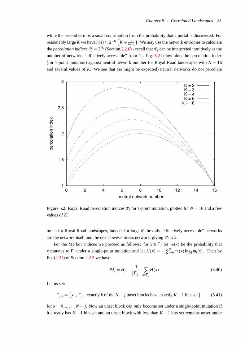
Chapter 5. ε-Correlated Landscapes81
while the second term is a small contribution from the probability that a portal is discovered. For
reasonably largeK we haveh(ε)≈ 2−K(
K + 1log2
). We may use the network entropies to calculate
thepercolation indicesP j = 2H j (Section2.2.6) - recall thatP j can be interpreted intuitively as the
number of networks “effectively accessible” fromΓ j . Fig. 5.2 below plots the percolation index
(for 1-point mutation) against neutral network number for Royal Road landscapes withN = 16
and several values ofK. We see that (as might be expected) neutral networks do not percolate
1
1.5
2
2.5
3
0 2 4 6 8 10 12 14 16
perc
olat
ion
inde
x
neutral network number
K = 2K = 3K = 4K = 6
K = 10
Figure 5.2: Royal Road percolation indicesP j for 1-point mutation, plotted forN = 16 and a few
values ofK.
much for Royal Road landscapes; indeed, for largeK the only “effectively accessible” networks
are the network itself and the next-lowest-fitness network, givingP j ≈ 2.
For the Markov indices we proceed as follows: forx ∈ Γ j let mi(x) be the probability that
x mutates toΓi under a single-point mutation and letH(x) = −∑Ni=0mi(x) log2mi(x). Then by
Eq. (2.21) of Section2.2.3we have:
M j = H j −1Γ j ∑
x∈Γ j
H(x) (5.40)
Let us set:
Γ j,k =
x∈ Γ j | exactlyk of theN− j unset blocks have exactlyK−1 bits set
(5.41)
for k = 0,1, . . . ,N− j. Now an unset block can only become set under a single-point mutation if
it already hasK−1 bits set and an unset block with less thanK−1 bits set remains unset under

Chapter 5. ε-Correlated Landscapes82
a single-point mutation. Thus, giveni, j,k, we see thatmi(x) is the samefor all x∈ Γ j,k, as is the
entropyH j,k = H(x). Thus:
M j = H j −N− j
∑k=0
Γ j,kΓ j H j,k (5.42)
A simple calculation gives:
mi(x) =j
Nδi, j−1 +
(1− j
N− k
L
)δi j +
kL
δi, j+1 (5.43)
for x∈ Γ j,k and: Γ j,kΓ j =
(N− j
k
)(Kε)k(1−Kε)N− j−k (5.44)
A calculation yields:
M j =(
1− jN
)h(ε)−
N− j
∑k=0
(N− j
k
)(Kε)k(1−Kε)N− j−k ·h
(kL
(1− j
N
)−1)
(5.45)
In particular, we see that:
M j ≤(
1− jN
)h(ε) (5.46)
so that (for fixedj) M j = O(ε logε) = O(K2−K
)asK→ ∞. Thus we might expect a maximum
entropy approximation to work well so long asK is large enough.
We may also use the Markov indices to calculate thepercolation drift factorsD percj = M j/H j
(Section2.2.6): the higher the factor, the more important drift becomes as regards accessibility
of neighbouring networks. We see that drift appears to be relatively unimportant - the percolation
drift factors are≈ 1 - but only for accessibility of other networks “in general”. However, as noted
in Section2.2.6, this is somewhat misleading as regards the importance of drift foroptimisation;
specifically, in this case the percolation drift factors tell us very little about the effect of drift
on accessibility ofhigher fitnessnetworks. We thus calculate theevolvabilitydrift factorsDevolj
(Eq.2.72). Eq. (4.3) then yields:
Devolj = 1−h
((1− j
N
)ε)−1 N− j
∑k=0
(N− j
k
)(Kε)k(1−Kε)N− j−k ·h
(kL
)(5.47)
Recall thatDevolj represents the fraction of information about the probability of finding a portal
from networkΓ j conveyed by knowledge of the actual sequence inΓ j . Fig. 5.3plots evolvability
drift factor (for 1-point mutation) against neutral network number for Royal Road landscapes with
N = 16 and several values ofK. We see that, particularly for larger block sizeK, a substantial
quantity of portal discovery information is conveyed by the knowledge of the actual location of a
sequence in a given network - for largeK (more specifically, forN 2K/K) we have roughly:
Devolj ≈ 1− log2L
K(5.48)
In fact, for a given neutral network on a Royal Road landscape, portals are accessible (for 1-bit
mutation) from only a sparse subset of the network. Neutral drift is thus likely to be essential for
the discovery of portals (cf. Chapter4).

Chapter 5. ε-Correlated Landscapes83
0
0.1
0.2
0.3
0.4
0.5
2 4 6 8 10 12 14
evol
vabi
lity d
rift f
acto
r
neutral network number
K = 2K = 3K = 4K = 6K = 8
K = 12
Figure 5.3: Royal Road evolvability drift factorsDevolj for 1-point mutation, plotted forN = 16
and few values ofK.

Chapter 5. ε-Correlated Landscapes84
Correlation properties
For Royal Road landscapes the mean fitnessF (d | j ) of an d-point mutant of a sequence se-
lected uniformly at random fromΓ j is given bydG(d)
j (z)dz
∣∣∣∣z=1
whereG(d)j (z) is given by Eq. (5.37)
and Eq. (5.39). The local correlation properties are contained in the quantityF (d | j ) (cf. Sec-
tion 2.3.1). Now:∂G j(z,u)
∂z
∣∣∣∣z=1
= j− [ j− (N− j)ε]θ(u) (5.49)
Settingw = u1−u in Eq. (5.39) and using Eq. (5.34) we find:
L
∑d=0
(Ld
)wdF (d | j ) = (N− j)ε(1+w)L +[ j− (N− j)ε] (1+w)L−K (5.50)
which yields:
F (d | j ) =
(N− j)ε+[ j− (N− j)ε]
(L−Kd
)/(L
d
)d≤ L−K
(N− j)ε d > L−K
(5.51)
We thus see that Royal Road landscapes arelinearly correlated(Section2.3.3). In particular, if
d L and (as assumed)ε 1 we have the approximation:
F (d | j )≈(
1− 1N
)d
j (5.52)
so that (to a first approximation) correlation does not depend on the block lengthK and Royal
Road landscapes are approximatelyelementary(Section2.3.2) with auto-correlation function:
ρ(d)≈(
1− 1N
)d
(5.53)
and hence correlation length:
` = N (5.54)
Optimal mutation mode
To test the accuracy of Prop.5.2.1 for Royal Road landscapes, we ran a series of Monte Carlo
simulations as follows: for each value ofN, K and network numberj and for a series of per-
sequence mutation rates, we generated a sample ofSuniform random sequences inΓ j . Each se-
quence was mutated according to the current mutation mode and the number of sequences which
found a portal toΓ j+1 totalled. 95% confidence limits were calculated according to Student’s
T-test (Feller, 1966). For each set of parameters the experiment was performed first forn-point
(constant) and then per-locus (Poisson) mutation. Results were plotted against the analytic ap-
proximations Eq. (5.4) and Eq. (5.5) for portal discovery probabilities forn-point and Poisson
mutation respectively - see Fig.5.4and Fig.5.5.
We see that for the larger block sizeK = 8 (Fig. 5.5) and particularly for smaller mutation
rates, the analytic results are in good agreement with experiment; less so for the smaller block
sizeK = 4 (Fig. 5.4) and larger mutation rates. This is to be expected as, firstly Eq. (5.4) and
Eq. (5.5) are only too(ε) = o(2−K
)and secondly the analysis relies on the (strong) multiplicative

Chapter 5. ε-Correlated Landscapes85
0
0.03
0.06
0.09
0.12
0 2 4 6 8 10 12
porta
l disc
over
y pr
obab
ility
per-sequence mutation rate
N = 12, K = 4, j = 2 constantPoisson
0
0.02
0.04
0.06
0 2 4 6 8 10 12
porta
l disc
over
y pr
obab
ility
per-sequence mutation rate
N = 12, K = 4, j = 4 constantPoisson
0
0.005
0.01
0.015
0.02
0.025
0 2 4 6 8 10 12
porta
l disc
over
y pr
obab
ility
per-sequence mutation rate
N = 12, K = 4, j = 8 constantPoisson
Figure 5.4: Portal discovery probability plotted against per-sequence mutation rate for a Royal
Road landscape with parametersN = 12, K = 4 and several values ofj = network number, forn-
point (constant) and per-locus (Poisson) mutation modes. Solid lines give the analytic values from
Eq. (5.4) and Eq. (5.5); the vertical arrows indicate the optimum mutation rates of Prop.5.2.1.
Points are values from a simulation with a sample size ofS= 100,000. Error bars give 95%
confidence limits.
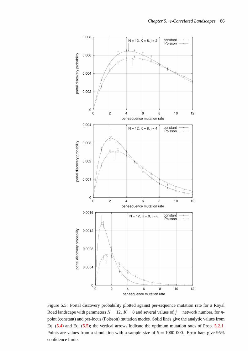
Chapter 5. ε-Correlated Landscapes86
0
0.002
0.004
0.006
0.008
0 2 4 6 8 10 12
porta
l disc
over
y pr
obab
ility
per-sequence mutation rate
N = 12, K = 8, j = 2 constantPoisson
0
0.001
0.002
0.003
0.004
0 2 4 6 8 10 12
porta
l disc
over
y pr
obab
ility
per-sequence mutation rate
N = 12, K = 8, j = 4 constantPoisson
0
0.0004
0.0008
0.0012
0.0016
0 2 4 6 8 10 12
porta
l disc
over
y pr
obab
ility
per-sequence mutation rate
N = 12, K = 8, j = 8 constantPoisson
Figure 5.5: Portal discovery probability plotted against per-sequence mutation rate for a Royal
Road landscape with parametersN = 12, K = 8 and several values ofj = network number, forn-
point (constant) and per-locus (Poisson) mutation modes. Solid lines give the analytic values from
Eq. (5.4) and Eq. (5.5); the vertical arrows indicate the optimum mutation rates of Prop.5.2.1.
Points are values from a simulation with a sample size ofS= 1000,000. Error bars give 95%
confidence limits.

Chapter 5. ε-Correlated Landscapes87
mutation approximation (Section2.2.4) which, as we have seen, is likely to apply if the Markov
index Eq. (5.45) is small. For the larger block size at least then, our results support Prop.5.2.1for
Royal Road landscapes, insofar as:
• Optimum mutation rates are correctly predicted
• The optimum portal discovery probability is higher for constant than for Poisson mutation
We remark that there is a fairly significant difference between the optimum portal discovery proba-
bilities for constant and Poisson mutation (the optimumrate for the latter is also generally higher).
As suggested in Chapter2 (Section2.3.4), there may be sound reasons, Prop.2.3.1and Prop.5.2.1
notwithstanding, to use Poisson mutation rather than a constant mutation mode on occasion.
The adaptive netcrawler on Royal Road landscapes
To test the adaptive netcrawler suggested in Section5.3.1on Royal Road landscapes, we tested
two schemes. They are both based, as suggested in Section5.3.1, on a working assumption that
the next-highest neutral network is ofequal neutralityto the current network. The first scheme is
based on the observation that under the above assumption theobservedneutrality should approach
1/e at the optimum mutation rate. Thus an estimateνobs of observed neutrality (i.e. proportion
of neutral mutations) is accumulated over the previoustlag fitness evaluations. At the end of
eachtlag evaluations,νobs is compared with 1/e. If it is smaller, the current mutation rate is
incremented; if larger the current mutation rate is decremented. This scheme, however, proved
to be somewhat unstable, in that the mutation rate tended to fluctuate wildly. We thus settled on
the following alternative scheme: a sliding estimateνobs of observed neutrality (i.e. proportion of
neutral mutations) is maintained over a “window” of the previoustlag fitness evaluations. After
each fitness evaluation the current mutation raten is updated according to:
n←[− nave
logνobs
](5.55)
wherenave is the average (arithmetic mean) of the actual mutation rate used over the previous
tlag fitness evaluations8. The idea is thatn tracks the optimum mutation rate, based on a sliding
estimate of actual neutrality, for a neutral network where the next-highest network is of equal
neutrality. We note that there are essentially two parameters involved: the “window” sizetlag and
the initial mutation rate. It proved judicious also to specify amaximummutation rate (which could
usually be taken to be the same as the initial mutation rate). In practice both parameters would
be tuned for best performance9. This latter scheme proved more stable and successful in tracking
the (known) optimum mutation rate. Fig.5.6illustrates a typical run. As might be expected (since
for Royal Road landscapes the next-highest network has somewhat smaller neutrality than the
current), there is a tendency to overestimate the optimum mutation rate - this may be seen clearly
8We have glossed over a subtlety here: the mutation rate is likely to be changing over the “window”. If the mutationrates over the window aren1,n2, . . . ,ntlag and tneut of the tlag evaluations are neutral, then the best estimate for theactualneutralityν is given by:νn1 +νn2 + . . .+νntlag = tneut. This equation is not (efficiently) solvable forν. However,sincen will not generally change too rapidly, using instead the arithmetic meannave proved sufficient and efficient toimplement.
9 In the case of Royal Road landscapes we in fact know that the (optimum) initial mutation rate, assuming a randomstart lands on the lowest network, is simply the block sizeN, so that in actual experiments we might allow ourselves tocheat a little...

Chapter 5. ε-Correlated Landscapes88
for the first few epochs in Fig.5.6. For general (unknown) landscapes for which one suspected
some relationship between fitness and neutrality (see e.g. the next Chapter), one might attempt
to correct this effect by the addition of a (possibly fitness-dependent) parameter to reduce slightly
the estimate of optimum mutation rate.
0
1
2
3
4
5
6
7
8
0 5000 10000 15000 200000
2
4
6
8
10
12
14
16
epoc
h
mut
atio
n ra
te (b
its)
fitness evaluations
epochactual
optimal
Figure 5.6: A typical run of an adaptive netcrawler (Section5.3.1) on a Royal Road fitness land-
scape. The horizontal axis measures fitness evaluations. The current epoch of the netcrawler (i.e.
current neutral network) is plotted against the left-hand vertical axis. Actual and optimal mutation
rates (in bits) are plotted against the right-hand vertical axis. Parameters are:N = 16, K = 12,
“window” size= 100 fitness evaluations, initial/maximum mutation rate= 16 (= N).
With the above proviso, we note that neither scheme depends on any knowledge of the un-
derlying fitness landscape; an adaptive netcrawler may be run on an arbitrary fitness landscape,
even if not known to be formallyε-correlated (but which may, in some sense, behave “locally” as
though it were). We return to this issue in the next Chapter.
5.4.2 Search performance on Royal Road landscapes
The principal contention of this Chapter is contained in Conjecture5.3.1- that a netcrawler with
the optimal (constant) mutation mode is the most effective evolutionary search process on anε-
correlated landscape. Here we put Conjecture5.3.1to the test on some Royal Road landscapes,
where we pit a netcrawler against some commonly encountered GA’s.

Chapter 5. ε-Correlated Landscapes89
Performance comparison
Firstly we establish a basis for comparison of search performance on Royal Road landscapes (cf.
Section3.5). For a full time/fitness-critical comparison we should have to compare the full dis-
tribution of Ti , the first passage time to networki or higher, for each networki (or equivalently
of X(t), the best-so-far network at timet, for all t within a reasonable range), for every set of
parameter values. This is unfeasible on grounds of time and space; we limit ourselves, then, to
the fitness-critical measuresE(Ti) and the time-critical measuresE(X(t)), remarking that simu-
lations (not illustrated) measuring the full distributions ofTi andX(t) do not change any of our
conclusions.
We are still, however, faced with the inevitability that our simulations can only run for a finite,
albeit large, maximum number of fitness evaluations,t∗, say. This is in particular a problem when
it comes to estimatingE(Ti) for the various search processes we shall be examining, since in any
given instantiation of a search process and for a giveni, our process may not have attained network
i within the maximum timet∗. Simply ignoring runs which do not reachi will not do; apart from
reducing the sample size we would also thus bias our estimate ofE(Ti). To address this problem
we make the following observation, borne out through many simulations and indeed for all search
processes tested: given a networki, for some suitably larget∗, the distribution ofTi given that
Ti > t∗ is similar to ageometricdistribution; i.e. fort > t∗ we haveP(Ti > t)≈ (1−λi)t for some
decay factorλi .
Consider, then, an experiment where we wish to estimate by sampling the meanE(T) of a
random variableT representing the first passage time of a processX(t) to a given statei. We
assume that there is some larget∗ and a decay factorλ such that fort > t∗ we haveP(T > t) ≈(1−λ)t . Suppose, now, that we runS instantiations of our processX(t), whereS is assumed large,
terminating each run att = t∗. Suppose that of theS runs, someS′ of them reach statei within
time t∗. We may then estimate:
p = P(T > t∗)≈ 1− S′
S≈ (1−λ)t∗ (5.56)
We then have:
P(T = t) = P(T = t | T ≤ t∗)P(T ≤ t∗)+P(T = t | T > t∗)P(T > t∗) (5.57)
= P(T = t | T ≤ t∗)P(T ≤ t∗)+P(T > t∗ | T = t)P(T = t) (5.58)
≈ P(T = t | T ≤ t∗)P(T ≤ t∗)+P(t > t∗)λ(1−λ)t−1 (5.59)
We thus find:
E(T)≈ E(T | T ≤ t∗)P(T ≤ t∗)+ p
(t∗+
1λ
)(5.60)
Now suppose that of theS′ samples which achieve statei within time t∗, the first passage times to
i aret1, t2, . . . , tS′ . We then have:
E(T | T ≤ t∗)≈ 1S′
(t1 + t2 + . . .+ tS′) (5.61)
which yields:
E(T)≈ 1S
(t1 + t2 + . . .+ tS′)+ p
(t∗+
1λ
)(5.62)
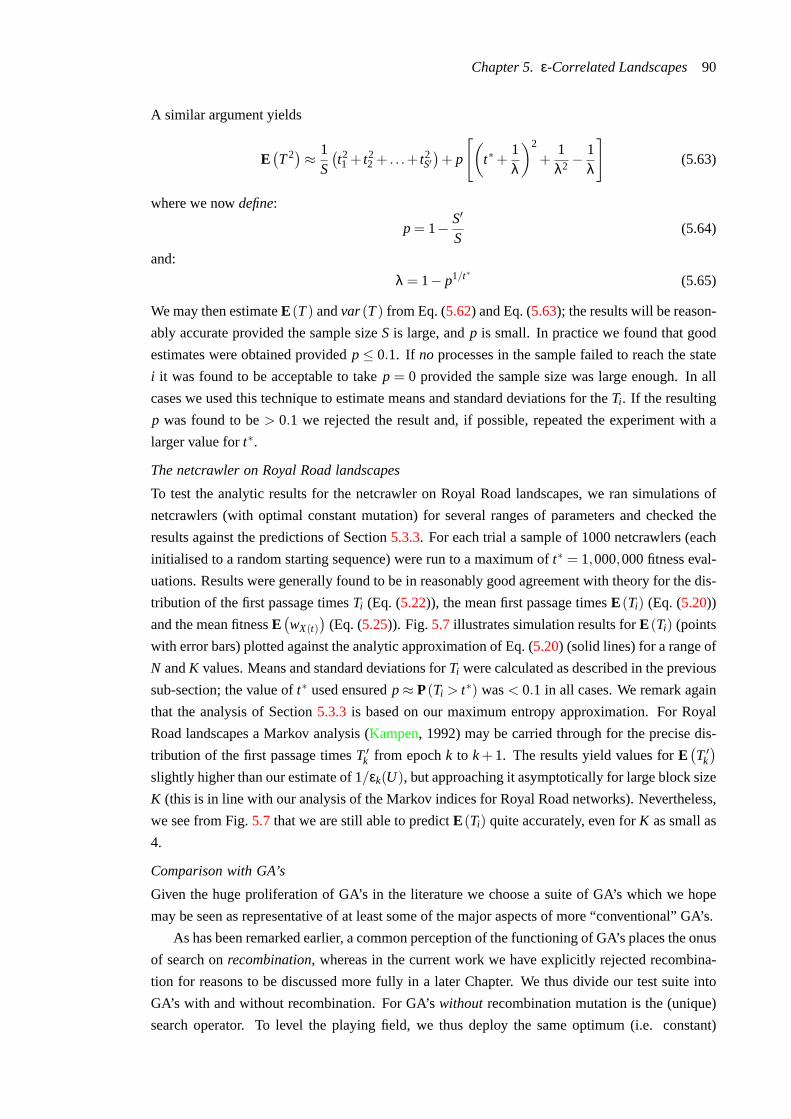
Chapter 5. ε-Correlated Landscapes90
A similar argument yields
E(T2)≈ 1
S
(t21 + t2
2 + . . .+ t2S′)+ p
[(t∗+
1λ
)2
+1λ2 −
1λ
](5.63)
where we nowdefine:
p = 1− S′
S(5.64)
and:
λ = 1− p1/t∗ (5.65)
We may then estimateE(T) andvar(T) from Eq. (5.62) and Eq. (5.63); the results will be reason-
ably accurate provided the sample sizeS is large, andp is small. In practice we found that good
estimates were obtained providedp≤ 0.1. If no processes in the sample failed to reach the state
i it was found to be acceptable to takep = 0 provided the sample size was large enough. In all
cases we used this technique to estimate means and standard deviations for theTi . If the resulting
p was found to be> 0.1 we rejected the result and, if possible, repeated the experiment with a
larger value fort∗.
The netcrawler on Royal Road landscapes
To test the analytic results for the netcrawler on Royal Road landscapes, we ran simulations of
netcrawlers (with optimal constant mutation) for several ranges of parameters and checked the
results against the predictions of Section5.3.3. For each trial a sample of 1000 netcrawlers (each
initialised to a random starting sequence) were run to a maximum oft∗ = 1,000,000 fitness eval-
uations. Results were generally found to be in reasonably good agreement with theory for the dis-
tribution of the first passage timesTi (Eq. (5.22)), the mean first passage timesE(Ti) (Eq. (5.20))
and the mean fitnessE(wX(t)
)(Eq. (5.25)). Fig.5.7illustrates simulation results forE(Ti) (points
with error bars) plotted against the analytic approximation of Eq. (5.20) (solid lines) for a range of
N andK values. Means and standard deviations forTi were calculated as described in the previous
sub-section; the value oft∗ used ensuredp≈ P(Ti > t∗) was< 0.1 in all cases. We remark again
that the analysis of Section5.3.3 is based on our maximum entropy approximation. For Royal
Road landscapes a Markov analysis (Kampen, 1992) may be carried through for the precise dis-
tribution of the first passage timesT ′k from epochk to k+ 1. The results yield values forE(T ′k)
slightly higher than our estimate of 1/εk(U), but approaching it asymptotically for large block size
K (this is in line with our analysis of the Markov indices for Royal Road networks). Nevertheless,
we see from Fig.5.7that we are still able to predictE(Ti) quite accurately, even forK as small as
4.
Comparison with GA’s
Given the huge proliferation of GA’s in the literature we choose a suite of GA’s which we hope
may be seen as representative of at least some of the major aspects of more “conventional” GA’s.
As has been remarked earlier, a common perception of the functioning of GA’s places the onus
of search onrecombination, whereas in the current work we have explicitly rejected recombina-
tion for reasons to be discussed more fully in a later Chapter. We thus divide our test suite into
GA’s with and without recombination. For GA’swithout recombination mutation is the (unique)
search operator. To level the playing field, we thus deploy the same optimum (i.e. constant)

Chapter 5. ε-Correlated Landscapes91
1
10
100
1000
10000
100000
1e+06
0 0.5 1 1.5 2 2.5 3 3.5 4
mea
n tim
e (fi
tnes
s ev
alua
tions
)
epoch
N = 4
K = 4K = 8K = 12K = 16 1
10
100
1000
10000
100000
1e+06
0 1 2 3 4 5 6 7 8m
ean
time
(fitn
ess
eval
uatio
ns)
epoch
N = 8
K = 4K = 8K = 12K = 16
1
10
100
1000
10000
100000
1e+06
0 2 4 6 8 10 12
mea
n tim
e (fi
tnes
s ev
alua
tions
)
epoch
N = 12
K = 4K = 8K = 12K = 16 1
10
100
1000
10000
100000
1e+06
0 2 4 6 8 10 12 14 16
mea
n tim
e (fi
tnes
s ev
alua
tions
)
epoch
N = 16
K = 4K = 8K = 12K = 16
Figure 5.7: Sample estimates of expected first passage timesTi for an (optimal) netcrawler on
Royal Road landscapes for a range ofN andK values. Vertical axes measure times in fitness eval-
uations, on a logarithmic scale. The horizontal axes specify the epoch (i.e. the network numberi).
Means (points) and standard deviations (error bars) were estimated using Eq. (5.62) and Eq. (5.63);
in all cases sample size was 1000 and the netcrawlers were run for 1,000,000 fitness evaluations
(which proved sufficient to ensure thatp< 0.1). Solid lines plot the theoretical estimate Eq. (5.20)
for E(Ti)

Chapter 5. ε-Correlated Landscapes92
mutation mode and rate for all such GA’s as for the netcrawler. For GA’swith recombination
we adopt the conventional view of recombination as the principal search operator, with mutation
as a “background” operator to maintain genetic diversity; we thus deploy a more conventional
(per-locus) mutation operator. Since it might be deemed unfair to match such a GA against an op-
timal netcrawler (where mutation rate/mode depends on knowledge of the landscape) we compare
performance in this case to anadaptivenetcrawler, as described in the previous sub-section.
In either scenario, where there are “tunable” parameters for our GA’s (including the adaptive
netcrawler) we take care to attempt, as far as possible, to tune parameters for optimal performance
on the given landscape and for the given performance criterion.
Key features of GA’s that we attempt to cover are:
• fitness-proportional vs. fitness rank selection
• multinomial sampling vs. stochastic universal sampling
• generational vs. “steady-state”
• one-point vs. uniform recombination
• enforced elitism
• fitness scaling
Of course we cannot be exhaustive; some commonly encountered schemes which we explicitly
exclude (on the grounds that they would lead us too far afield) include:
• distributed GA’s
• associative (and other) mating schemes
• nicheing/fitness sharing
The final list of population-based GA’s to be matched against a netcrawler was as follows:
FP Fitness-proportional selection
RANK Fitness rank selection
2TWRL 2-Tournament winner-replaces-loser
The “generational” GA’s FP and RANK were run with either multinomial (roulette-wheel) sam-
pling (MNS) or stochastic universal (roulette-wheel) sampling (SUS) and also both with and with-
out enforced elitism. FP and RANK were also run with either linear (LIN), power law (POW) or
exponential (EXP) scaling10 - for FP, the actual fitness is scaled, while for RANK the fitnessrank
is scaled (see below). With recombination, 1-point, 2-point anduniformcrossover were trialled.
We firstly describe the generational GA’s FP and RANK. Scaling was performed as follows:
a scale factorparameters> 0 controls the selection pressure. For linear scaling (LIN) the scaled
“roulette-wheel sector size” is given by:
xscaled= x+s (5.66)
10We did not implement the so-called “sigma-scaling” (Mitchell et al., 1992;Goldberg, 1989) often encountered inthe literature.

Chapter 5. ε-Correlated Landscapes93
For power law scaling (POW) the scaled size is given by:
xscaled= (x+1)s (5.67)
an for exponential scaling (EXP) the scaled size is given by:
xscaled= esx (5.68)
wherex represents the fitness (x = 0,1,2, . . . ,N) for fitness-proportional selection (FP) and the fit-
ness rank number in the population, minus one (x = 0,1,2, . . . ,M−1) for rank selection (RANK).
Note that for linear scaling increasings reducesselection pressure, while for power law and ex-
ponential scaling increasings increasesselection pressure. If we take as a measure of selection
pressure the ratio xscaled(x−1)scaled
of a sector to the next-smallest (possible) sector, we find, for a sector
of sizex, selection pressures of 1+ 1x+s−1,
(1+ 1
x
)sandes for LIN, POW and EXP respectively.
Note that for LIN and POW, for a given scale factors, selection pressure decreases (approaching
1 from above) with increasing sector sizex, while for EXP it remains constant.
Both FP and RANK selection utilise a simulated a roulette-wheel. For FP each population
member is allocated a sector of size equal to its scaled fitness. For RANK the population is
sorted11 into (ascending) rank order by fitness and each population member is allocated a sector
of size equal to its scaled rank. For multinomial sampling (MNS) selections are performed so that
for any selection event theprobability of selecting a given population member is proportional to
its sector size (thus so too is itsexpectednumber of selections). For stochastic universal sampling
(SUS) (Baker, 1987) selections are performed such that, given a fixed number of selections (gen-
erally equal to the population size), theexpectednumber of selections of a population member is
proportional to its sector size and thevariancein its selection probability is minimal.
In the limit of very high scale factors (for power law and exponential scaling), the interplay
with selection is as follows: for FP selection the entire roulette-wheel is allocated equally among
thehighest fitnesssequences in the population. Thus MNS sampling amounts to uniform random
selections from the highest fitness sequences, while SUS sampling yields (approximately) equal
numbers of selections foreachof the highest fitness sequences. For RANK selection,one of
the highest fitness sequences is chosen uniformly at random (cf. the previous footnote regarding
shuffling of the population prior to sorting); the entire roulette-wheel is then allocated to this single
sequence, which consequently receivesall samples, for both MNS and SUS sampling. Frequently
in seeking optimal GA settings, it became clear that performance increased toward the maximum
scale factor limit. Due to floating-point storage limitations, if a scale factor was> 30 (POW) or
> 10 (EXP) the limiting case was assumed (cf. Table5.1).
With no recombination, the generational GA’s operate as follows. Population size isM. For the
initial generationM sequences are created at random. For each subsequent generationM selections
are performed according to the operant selection/sampling method. Each selected sequence is
mutated (according to the theoretical optimal mode/rate for the selected sequence; i.e. according
to its neutral network) and added to a new population. AfterM such selections the new population
replaces the old to become the current population.
11Implementation note: before sorting the population isshuffled. This avoids the possibility that the sorting algorithm- qsort in our case - always rankequally fitsequences in the same order - which would, of course, violate the Markovproperty of the evolutionary process!

Chapter 5. ε-Correlated Landscapes94
With recombination there is an additionalrecombination rateparameter 0≤ r ≤ 1 and amu-
tation rateparameter ¯u equal to the expected number of mutations per sequence, although (for
reasons given above) mutation is now on aper-locus basis12. Again an initial random population
of sizeM is created. For each generation we again performM selections. This time, after each
selection, with probabilityr a recombination event occurs and an additional “parent” sequence is
selected. This parent selection is somewhat different for MNS and SUS sampling: in the former
case another roulette-wheel selection is performed, while in the latter case a uniform random se-
lection is made from the current population13. The selected parents are crossed over according to
the crossover mode (1-point, 2-point or uniform), mutated14 and added to the new population as
before.
For the “steady-state” tournament GA 2TWRL (Chapter3, Example3.2.2) again an initial
population of sizeM is created at random. The following procedure is then iterated: two sequences
are selected uniformly at random and without replacement from the population for a “tournament”.
The tournament winner is declared to be the fitter (or, if the selections are of equal fitness, the first)
of the two selections. If there is no recombination a copy of the winner is then mutated and the
mutant copy replaces the tournament loser. If there is recombination then with probabilityr the
winner crosses over with the loser and the offspring mutates and again replaces the loser. Note that
2TWRL is “almost”elitist insofar as, if there is just one maximally fit sequence in the population,
then the only way that sequence might be eliminated at the expense of a less fit sequence is if it is
selected twice for a tournament (so it becomes both winner and loser...) and then mutates (and/or
mates) to produce an inferior offspring which replaces itself! We note that if selections for the
tournament were performedwithout replacement then the process would be strictly elitist.
In the case of recombination, it was found that 2-point and (more markedly so) uniform
crossover were invariably inferior in performance compared to the corresponding process with
1-point crossover. This is reasonable, if we consider that uniform recombination (and to a lesser
extent 2-point crossover) is more likely to destroy already set blocks. We therefore present results
for 1-point crossover only.
As regards elitism, we found that enforcing any form of “pure” elitism - i.e. ensuring that we
never lose all of the current fittest sequences - merely reinforced the main thesis of this Chapter
rather strongly, in that performance generally favoured smaller population sizes (and smaller re-
combination rates). In particular, best results were always obtained with a population size of 1
and a recombination rate of 0 - in which case the corresponding GA simply became a netcrawler!
Results involving explicitly imposed elitism are thus omitted.
Simulations were performed for a Royal Road landscapes withN = 8 andK = 8 as follows: for
each GA the process was simulated 1,000 times (with different random seeds15) from random ini-
tial populations up to 10,000 fitness evaluations. For each time (number of fitness evaluations) the
12Although we mutate on a per-locus basis, we still prefer - contrary to common practice in the GA literature - toquote mutation rates as an (expected) per-sequence rate as, in the author’s view, this is a more meaningful figure. Thereader irritated by this practice may feel free to avail them self of a pocket calculator...
13The reason for this is that SUS sampling presupposes afixednumber of selections per generation. Other schemesare of course feasible, but for simplicity we choose random “other parent” selection.
14We note that some GA practitioners (Michaelewicz, 1996) prefer to separate recombination and mutation; i.e. asequenceeithermatesor mutates. The practical difference proved minimal in our case.
15For pseudo-random number generation we used the “Mersenne Twister” (Matsumoto & Nishimura, 1998) RNG.

Chapter 5. ε-Correlated Landscapes95
sample mean best-so-far fitness over the 1,000 runs was calculated16. Standard deviations in best-
so-far fitness (not shown) were also calculated (the relative deviation= standard deviation/actual
fitness tended to range between 5%−15%). Great care was taken to tune the various parameters
(population size, scale factors, recombination rates and mutation rates) for best performance over
the alloted 10,000 evaluations, where the mean best-so-far fitness at 10,000 evaluations was taken
as the performance indicator. Results are displayed in Fig.5.8 and Fig.5.9 with optimised pa-
rameters as in Table5.1 and Table5.2 respectively. For comparison, (theoretical) random search
results and (simulated) optimised/adaptive netcrawler results are shown alongside.
We remark that for reasons of time and space we have presented results only for a Royal Road
landscape withN = 8 andK = 8. This proved quite representative - other Royal Road landscape
parameters did not spring any surprises, provided the block sizeK was reasonably large.
selection sampling scaling scale pop. performance
method method method factor size indicator
ONC − − − 1 7.911
RSH − − − 1 2.018
FP MNS LIN 0.00 100 4.632
FP MNS POW max 45 7.673
FP MNS EXP max 35 7.713
FP SUS LIN 0.00 100 4.809
FP SUS POW max 50 7.694
FP SUS EXP max 50 7.756
RANK MNS LIN 0.00 80 3.025
RANK MNS POW 15.00 55 7.339
RANK MNS EXP 0.16 80 7.207
RANK SUS LIN 0.00 80 3.133
RANK SUS POW 16.00 50 7.420
RANK SUS EXP 0.19 70 7.355
2TWRL − − − 20 7.052
Table 5.1: Optimised GA parameters and results (no recombination), on a Royal Road landscape
with N = 8, K = 8. ONC = optimal netcrawler, RSH = random search - see text for other ab-
breviations. The final columnperformance indicator= mean best-so-far fitness at 10,000 fitness
evaluations. For scale factors marked “max” see text.
We give a brief discussion of the results, beyond pointing out that they generally support our
contention well that the (optimised/adaptive) netcrawler yields optimum performance on Royal
Road (and, we would claim,ε-correlated) landscapes. We remark in particular that it is clear from
the results that, while some GA’s came close in performance under the time-critical “mean best-so-
far fitness att∗ evaluations” indicator fort∗ = 10,000, those GA’s had to be finely tuned to achieve
good performancefor that particular time scale; the netcrawler frequently outperformed thesame
16Note that even for the generational GA’s we count fitness evaluations strictly sequentially, in the sense that at eachactual fitness evaluation - i.e. after a mutation, a recombination or (in the initialisation phase) a random creation - wecheck if we have discovered a new best-so-far fitness.

Chapter 5. ε-Correlated Landscapes96
0
1
2
3
4
5
6
7
8
0 2000 4000 6000 8000 10000
mea
n fit
ness
time (fitness evaluations)
ONCRSH
FP MNS LINFP MNS POWFP MNS EXP
FP SUS LINFP SUS POWFP SUS EXP
RANK MNS LINRANK MNS POWRANK MNS EXP
RANK SUS LINRANK SUS POWRANK SUS EXP
2TWRL
1
2
3
4
5
6
7
8
ONC FPSUSEXP
FPMNSEXP
FPSUSPOW
FPMNSPOW
RANKSUSPOW
RANKSUSEXP
RANKMNSPOW
RANKMNSEXP
2TWRL FPSUSLIN
FPMNSLIN
RANKSUSLIN
RANKMNSLIN
RSH
mea
n fit
ness
Figure 5.8: Optimised GA performance (no recombination) on a Royal Road landscape with
N = 8, K = 8: mean best-so-far fitness (sample size 1,000 runs) plotted against time in fitness
evaluations. See text and Table5.1 for key and parameters. The bottom figure shows a histogram
of mean best-so-far fitness at the end of each run, ranked by performance.

Chapter 5. ε-Correlated Landscapes97
0
1
2
3
4
5
6
7
8
0 2000 4000 6000 8000 10000
mea
n fit
ness
time (fitness evaluations)
ANCRSH
FP MNS LINFP MNS POWFP MNS EXP
FP SUS LINFP SUS POWFP SUS EXP
RANK MNS LINRANK MNS POWRANK MNS EXP
RANK SUS LINRANK SUS POWRANK SUS EXP
2TWRL
1
2
3
4
5
6
7
8
ANC RANKMNSEXP
RANKMNSPOW
FPMNSPOW
FPMNSEXP
RANKSUSPOW
RANKSUSEXP
2TWRLRANKMNSLIN
FPSUSPOW
FPSUSEXP
RANKSUSLIN
FPMNSLIN
FPSUSLIN
RSH
mea
n fit
ness
Figure 5.9: Optimised GA performance (with recombination) on a Royal Road landscape with
N = 8, K = 8: mean best-so-far fitness (sample size 1,000 runs) plotted against time in fitness
evaluations. See text and Table5.2 for key and parameters. The bottom figure shows a histogram
of mean best-so-far fitness at the end of each run, ranked by performance.
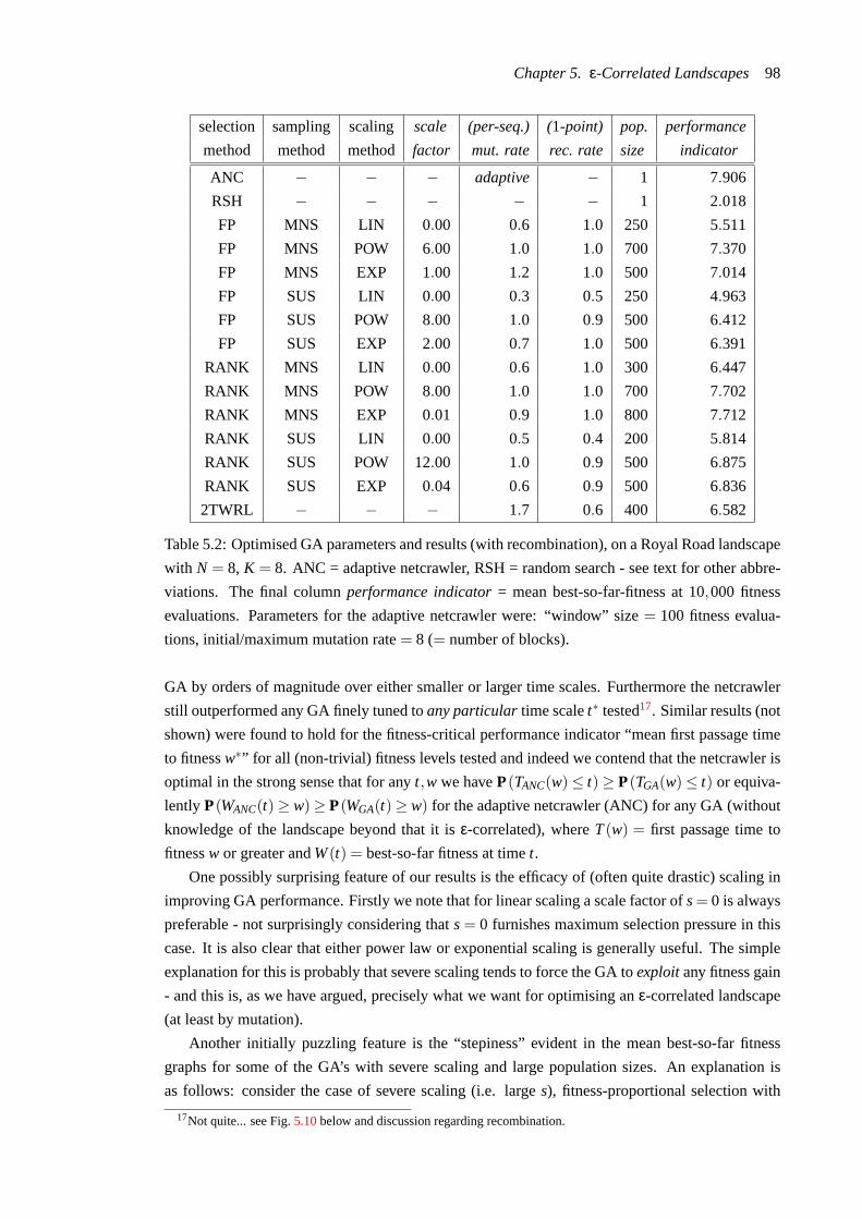
Chapter 5. ε-Correlated Landscapes98
selection sampling scaling scale (per-seq.) (1-point) pop. performance
method method method factor mut. rate rec. rate size indicator
ANC − − − adaptive − 1 7.906
RSH − − − − − 1 2.018
FP MNS LIN 0.00 0.6 1.0 250 5.511
FP MNS POW 6.00 1.0 1.0 700 7.370
FP MNS EXP 1.00 1.2 1.0 500 7.014
FP SUS LIN 0.00 0.3 0.5 250 4.963
FP SUS POW 8.00 1.0 0.9 500 6.412
FP SUS EXP 2.00 0.7 1.0 500 6.391
RANK MNS LIN 0.00 0.6 1.0 300 6.447
RANK MNS POW 8.00 1.0 1.0 700 7.702
RANK MNS EXP 0.01 0.9 1.0 800 7.712
RANK SUS LIN 0.00 0.5 0.4 200 5.814
RANK SUS POW 12.00 1.0 0.9 500 6.875
RANK SUS EXP 0.04 0.6 0.9 500 6.836
2TWRL − − − 1.7 0.6 400 6.582
Table 5.2: Optimised GA parameters and results (with recombination), on a Royal Road landscape
with N = 8, K = 8. ANC = adaptive netcrawler, RSH = random search - see text for other abbre-
viations. The final columnperformance indicator= mean best-so-far-fitness at 10,000 fitness
evaluations. Parameters for the adaptive netcrawler were: “window” size= 100 fitness evalua-
tions, initial/maximum mutation rate= 8 (= number of blocks).
GA by orders of magnitude over either smaller or larger time scales. Furthermore the netcrawler
still outperformed any GA finely tuned toany particulartime scalet∗ tested17. Similar results (not
shown) were found to hold for the fitness-critical performance indicator “mean first passage time
to fitnessw∗” for all (non-trivial) fitness levels tested and indeed we contend that the netcrawler is
optimal in the strong sense that for anyt,w we haveP(TANC(w)≤ t)≥ P(TGA(w)≤ t) or equiva-
lently P(WANC(t)≥ w)≥ P(WGA(t)≥ w) for the adaptive netcrawler (ANC) for any GA (without
knowledge of the landscape beyond that it isε-correlated), whereT(w) = first passage time to
fitnessw or greater andW(t) = best-so-far fitness at timet.
One possibly surprising feature of our results is the efficacy of (often quite drastic) scaling in
improving GA performance. Firstly we note that for linear scaling a scale factor ofs= 0 is always
preferable - not surprisingly considering thats= 0 furnishes maximum selection pressure in this
case. It is also clear that either power law or exponential scaling is generally useful. The simple
explanation for this is probably that severe scaling tends to force the GA toexploitany fitness gain
- and this is, as we have argued, precisely what we want for optimising anε-correlated landscape
(at least by mutation).
Another initially puzzling feature is the “stepiness” evident in the mean best-so-far fitness
graphs for some of the GA’s with severe scaling and large population sizes. An explanation is
as follows: consider the case of severe scaling (i.e. larges), fitness-proportional selection with
17Not quite... see Fig.5.10below and discussion regarding recombination.

Chapter 5. ε-Correlated Landscapes99
multinomial sampling and a large population sizeM. After the random initial population stage
(generation 0) suppose that the highest network found isj0 and that, say,k members in the initial
population are on thej0 network. During the next generation (generation 1), thosek sequences
dominate the roulette-wheel to the extent that every selection is more or less a uniform sample of
thosek sequences. Suppose that there is no recombination. Each of thek selectees mutates with
a certain probability of finding a portal to networkj0 + 1. There is a reasonable chance, if the
population is large, that (at least) one such mutant does so - but there is only a tiny chance (by the
nature ofε-correlation) that any mutant finds a portal to a networkhigher than j0 +1. As a result,
we can expect the best-so-far fitness to change (quite early on in the generation for smallj0) from
j0 to j0+1 - and then to stay there. This theme is then repeated for the next generation (generation
2) at j0 + 1, and so on. The “stepiness” decreases with increasing fitness, since for higherj the
probability of finding a portal toj +1 becomes smaller and so portals tend to be discoveredlater
during a generation (or not at all, so that the averaged out “steps” begin to overlap). We would
expect (and indeed find) a similar effect with other sampling methods (SUS) and with fitness
ranking (in this case only the top-ranked sequence (onj0, of course) is repeatedly selected, but
the effect is similar. Something analogous also appears to occur with recombination, even at small
mutation rates (see below). The prerequisite is that it be “easy” to find (by whatever means) a
portal to the next step up but “difficult” to find a portal to anyhigher step. These conditions
appear to exist too for recombination. We would not expect (and indeed do not find) the effect in
our steady-state GA.
Although not the point of this Chapter, we do have some interest in the utility of recombina-
tion in our GA’s. By and large they support well the conclusions of (Forrest & Mitchell, 1993),
a landmark study of the efficacy of recombination and theBuilding Block Hypothesis(Chapter7,
Section7.1) on Royal Road landscapes. They found similarly that their GA’s were invariably
outperformed by a “Random Mutation Hill-Climber” (RMHC) - basically our netcrawler with
constant 1-bit mutation. Their analysis of the reasons for the GA’s poor performance - in particu-
larly the apparent failure of recombination to splice together sequences with different set blocks as
per the Building Block Hypothesis - fingershitch-hiking(Chapter7, Section7.2) as the principal
culprit. This is the phenomenon, long known to population genetics, whereby whenever a geno-
type in a population discovers a “good gene”, that genotype (and its identical-but-for-mutation
progeny), rapidly take over the population with all its “bad genes” in tow, thus leaving insufficient
genetic variation for recombination to work with. In effect, there rarelyaresequences withdiffer-
entgood genes simultaneously in a population and recombination has nothing to splice together.
Thus we may well ask what role recombination is fulfilling in our GA’s. Firstly, we note that the
optimised parameters generally have ahigh recombination rate (frequently near 1 and occasion-
ally, amusingly, near the folkloric “magic” rate of 0.6 (Michaelewicz, 1996). This implies that
recombination is at least not a hindrance to our GA; quite the opposite, in fact.
To test the efficacy of (1-point) recombination we ran several of our GA’s with a recombination
rate of 1 and a mutation rate of 0; this is, perhaps, a “Big Bang” GA (Chapter3, Section3.4) in
its purest form - optimisation will (hopefully) continue until there is insufficient genetic variation
(which may be lost through stochastic sampling or may not have been present in the initial random
population) for recombination to be effective. The situation appears complex, but it appears that

Chapter 5. ε-Correlated Landscapes100
with careful tuning of selection pressure (“exploitation”, but danger of hitch-hiking and running
out of diversity too quickly) and population size (“exploration”, but danger of wastefulness) quite
good results may be achieved - but parameters, as pointed out above, have to be finely tuned to
meet specific time/fitness criteria. Fig.5.10demonstrates the “exploit/explore” (Holland, 1992)
trade-offs involved. In summary, while it is clear that (1-point) recombinationcan put together
“building blocks” very effectively on a Royal Road landscape18 - indeed, this was theraison
d’etre for their design - it seems difficult to exploit this capability in a GA (Mitchell et al., 1994)
to the extent that it can compete with an (optimised/adaptive) netcrawler.
We note finally that the adaptive netcrawler achieves a performance almost as good as the
optimal netcrawler and that tuning was quick and simple - there seems to be a large “sweet spot”
in the parameter values (primarily the “window” size), which are also, happily, rather insensi-
tive to time/fitness scales. In contrast, tuning the parameters of the population GA’s was (as any
GA practitioner will verify...) a tedious and time-consuming task - while parameters sometimes
exhibit large “sweet spots” they very frequently turn out to be sensitive, difficult to predict and
interact “synergistically” (i.e. performance appears to depend on highly non-linear combinations
of parameters), as well as depending critically on the time/fitness scale for which one wishes to
optimise performance. Population size in particular seemed often to be quite tightly related to the
time scale, particularly with severe scaling and recombination (see above for a partial explana-
tion). We note with interest that an analytical study on the related “Royal Staircase” landscapes by
(Nimwegen & Crutchfield, 1998) reaches a seemingly opposite conclusion, noting a large “sweet
spot” in population size and mutation rates for a simple fitness-proportional GA (without recombi-
nation). However the performance measure in that study is the (fitness-critical) first passage time
to achieve maximum fitness as opposed to our (time-critical) best-so-far fitness measure, so - quite
apart from the landscape differences - we shouldn’t expect comparable qualitative behaviour.
5.5 Discussion
In this Chapter we introduced the statistical property ofε-correlation to describe landscapes with
neutral networks for which higher networks are accessible only from the current network. For such
landscapes we have calculated (Prop.5.2.1) the optimal mutation mode/rate and argued (Conjec-
ture5.3.1) that there is also an optimal evolutionary search strategy which is not population-based
but rather a form of hill-climber which we have dubbed thenetcrawler. On the basis of these
results we have proposed a heuristic - the 1/e Neutral Mutation Rule(Prop.5.3.1) - which we
claim to have more general application on fitness landscapes with neutral networks. We have
also proposed anadaptivevariant of the netcrawler which gathers statistical information about the
landscape as it proceeds and uses this information to self-optimise.
We remark that a major motivation for the research presented in this study was a series of ex-
periments by Thompson and Layzell in on-chip electronic circuit design by evolutionary methods
(Thompson & Layzell, 2000), during which an algorithm almost identical to our netcrawler was
used with some success. The mutation rate deployed in these experiments, albeit chosen on heuris-
tic grounds different from ours, in fact turns out to be almost precisely the optimal rate predicted
18So well, in fact, that in Fig.5.10(top figure, pop. size= 100) we see that for (very) short time scales/low fitnessrecombination actually slightly outperforms the adaptive netcrawler...

Chapter 5. ε-Correlated Landscapes101
0
1
2
3
4
5
6
7
8
0 2000 4000 6000 8000 10000
mea
n fit
ness
time (fitness evaluations)
ANCRSH
M = 100M = 1000M = 1900
0
1
2
3
4
5
6
7
8
0 2000 4000 6000 8000 10000
mea
n fit
ness
time (fitness evaluations)
ANCRSHs = 1
s = 11s = 21
Figure 5.10:Recombination only: performance of a fitness-proportional GA with multinomial
sampling and power law scaling on a Royal Road landscape withN = 8, K = 8: mean best-so-
far fitness (sample size 1,000 runs) plotted against time in fitness evaluations. In the top figure
selection pressure is high (scale factor= 10) and population size is varied. In the bottom figure
population size is high (= 1,000) and selection pressure is varied.

Chapter 5. ε-Correlated Landscapes102
here, given the (estimated) neutrality inherent in the problem. There is, we note, no particular ev-
idence that the fitness landscape in these experiments isε-correlated to any degree; indeed, work
in progress by the author suggests that the principal results presented in this Chapter may obtain
under considerably less stringent assumptions (cf. Chapter6) thanε-correlation.

Chapter 6
The NKp Family of Random Fitness Landscapes
6.1 Background
The NK family of random fitness landscapes were introduced by Stuart Kauffman (Kauffman
& Levin, 1987;Kauffman, 1989;Kauffman, 1993) as a statistical model to investigate the phe-
nomenon ofepistasis- where the effect on fitness of substituting an allele at some locus depends
on the particular alleles at other loci on the genotype. While this phenomenon had long been
recognised by population geneticists (S. Wright, 1932) it tended either to be absent or vastly over-
simplified in their models. Kauffman’s model, it might be said, is more in line with random energy
models from statistical mechanics, (eg.spin glasses(Sherrington & Kirkpatrick, 1975;Anderson,
1985)) or from combinatorial optimisation (eg. Travelling Salesman problem (Lawler, Lenstra,
Kan, & Shmoys, 1985), graph bi-partitioning (Fu & Anderson, 1986),etc.) than standard pop-
ulation genetics models. The gist of Kauffman’s construction is to abstract away the details of
how genotype maps to fitness - that mapping is deemed unknown and inscrutable and is therefore
(in the spirit of statistical mechanics) modelled as a random mapping - except that this random
mapping assumes a degree of epistasis in that fitness depends (additively) on contributions from
overlapping groups of “epistatically linked” loci. Crucially, the degree of epistasis in the NK
model can be “tuned” by means of theK parameter, making NK landscapes a candidate test bed
for investigating the effects of epistasis.
The emphasis in Kauffman’s analysis was on the“ruggedness”or correlation properties of
NK landscapes arising from epistatic interactions of loci and on how this ruggedness mediates
the behaviour of evolutionary processes. The NK model was extended in (Barnett, 1997;Barnett,
1998) to the NKp family of landscapes, to incorporate the phenomenon ofselective neutrality
(Section1.2). The key feature of the NKp model turns out to be the “statistical independence”,
in a sense to be made precise below, of epistasis (as tuned by theK parameter) and neutrality (as
tuned by thep parameter), making NKp landscapes a candidate test bed for investigating the ef-
fects and interaction of epistasis and neutrality. NKp landscapes featureneutral networksalthough
(probably) not, it should be remarked, structurally similar to those of the RNA folding landscapes
which inspired the concept - indeed, (arguably) more realisticrandom graphstatistical models
(Reidys, 1995;Reidys et al., 1997) have been developed to investigate the neutral network struc-

Chapter 6. The NKp Family of Random Fitness Landscapes104
ture of RNA folding landscapes. NKp landscapes, thus, do not set out to model these landscapes
but might (we shall argue) merit consideration as models for fitness landscapes arising inartifi-
cial evolution/optimisation. They might, at least, serve as an aid to intuition for the structure and
evolutionary dynamics on fitness landscapes featuring both epistasis and selective neutrality.
NK landscapes (and NKp landscapes) have been placed in the more general context ofrandom
additive landscapesby (Reidys & Stadler, 2001) in which the statistical properties of epistasis and
neutrality may be analysed. In this Chapter we do generalise somewhat the original NK (and NKp)
constructions but concentrate more on properties specific to these landscapes. We remark that we
approach the concept of “random fitness landscape” in the “constructive” (rather than the more
mathematically rigorous “prescriptive”) fashion outlined in Chapter 2.
We note that the basic NKp landscape construction was originally introduced in (Barnett,
1997), where the statistical independence of epistasis and neutrality was also conjectured (to be
proved rigorously by (Reidys & Stadler, 2001)). A few further statistical results on NKp land-
scapes were presented in (Barnett, 1998); nonetheless, the majority of the analysis in the this
Chapter represents new research.
A note on notation and terminology
As regards notation, we forsake compatibility with the literature in the interests of internal con-
sistency; in particular, we retain the notationw, w′, etc. for fitness values (rather thanx, y, . . .)
andW, W′, . . . (rather thanX, Y, . . .) for random variables representing fitness values. We shall,
furthermore, continue to writeL for sequence length, rather thanN as implied by the notation
“NK”. We shall also, for convenience, use the term“arbitrary” in a specific technical sense, to
mean“drawn from a uniform random distribution”from some set (which will generally be clear
from the context). In particular, throughout this Chapter the random variableW will denote the
fitness of an arbitrary sequence (i.e. one drawn uniformly at random) from a sequence spaceAL.
6.1.1 Construction
The Generalised NKp Model
In Kauffman’s original scheme for NK landscapes (Kauffman, 1993) each locus on a sequence of
lengthL contributes additively to the fitness of that sequence. The contribution of a locus, drawn
(independently and at random) from some underlying distribution, then depends on the allele at
the locus itself and the alleles at some otherK (randomly chosen) loci. While in a biological
context there may be some justification for considering fitness contributions on a per-locus basis,
this seems less obvious if we intend to use the NK scheme to model an artificial evolution fitness
landscape. Rather, we introduce a variation on the NK theme as follows: suppose that the fitness
of a potential candidate for the solution of an optimisation problem depends, via some genotype
→ phenotype mapping, on some set ofF featuresof the phenotype. For example, in attempting to
evolve a neural network controller for a robot that is required to perform a specified task, we might
consider the neural network design to be the “phenotype”, while the “features” might be higher
level robot “behaviours” associated with the phenotype (e.g.move towards light, avoid collision
with object, etc.), on which fitness is ultimately evaluated. Now the sequence→ feature mapping
may be assumed complex and inscrutable - otherwise we would probably not bother applying
artificial evolution to our problem! We thus, in the spirit of the standard NK model, assume (i)

Chapter 6. The NKp Family of Random Fitness Landscapes105
that ourF features contribute additively and independently towards fitness; (ii) that thefitness
contribution of a feature depends on the alleles at some subset of loci of a sequence - we shall say
that a locusinfluencesa feature if the fitness contribution of that feature depends on the choice
of allele at that locus - and (iii) for each combination of alleles at the influencing loci the fitness
contribution of a feature is drawn independently from someunderlying distribution (i.e. real-
valued random variable)Z. As yet we make no assumptions about the assignation of influencing
loci nor about the underlying distribution.
Epistasis in the NK Model
We now make the assumption that the loci influencing a given feature are chosen independently
per feature1 and define theepistasis parameterκ to be the probability that an (arbitrary) locus
influence an (arbitrary) feature. We do allow some flexibility in the choice of loci that influence a
feature; in particular, we shall consider thefixed epistasismodel, where each feature is influenced
by exactlyK loci, chosen uniformly at random from theL possible loci (so thatκ = K/L) and the
variable epistasismodel where, for each feature, the probability that it be influenced by a locus
is decided (independently for each locus) by a biased coin-toss with probabilityκ. There are,
of course, other possible choices for assigning epistasis (e.g. the “nearest neighbour” scheme in
(Kauffman, 1993)); as we shall see, however, the significant quantity2 will turn out to be simply
thenumberof loci that influence an arbitrary feature. We note that the fixed epistasis model with
F = L corresponds3 to the standard NK model with “fully random” epistasis (Kauffman, 1993;
Altenberg, 1995).
The Generalised NKp Model
We shall also extend our generalised NK model to include (a generalisation of) the NKp landscapes
(Barnett, 1997). The motivation for the NKp construction is that it seems reasonable to suppose
that for many (if not most) combinations of alleles at the loci influencing a feature, that feature will
be “ineffective” in the sense that it will make azero contributionto overall fitness. Specifically,
in the spirit of the NK model, we suppose that a feature make a zero contribution - independently
for any combination of alleles at the influencing loci - with fixed probability 0≤ p < 1 so that the
underlying fitness distributionZ takes the form:
Z =
0 with probability p
Y with probability q≡ 1− p(6.1)
whereY is a continuous, non-atomic4 (Feller, 1966) real-valued random variable. In other words,
for each feature and for each particular combination of alleles at the influencing loci, whether that
feature makes a zero contribution is decided on a biased coin-toss controlled by theneutrality
parameter0≤ p≤ 1. Neutrality is (as we shall see) zero forp = 0 and increases with increasing
p. The casep = 0 yields (almost surely) a trivial landscape where every sequence has fitness 0.
NKp landscapes are thus specialisations of generalised NK landscapes. When discussing NKp
1One might, alternatively, choose the features influenced by a given locus independentlyper locus. Our choice isbased on analytic tractability and simplicity of (computer) implementation.
2At least in the absence of any consideration ofrecombination.3Almost... in the usual NK construction a locus always “influences itself”.4I.e. P(Y = w) = 0 for anyw∈ R.

Chapter 6. The NKp Family of Random Fitness Landscapes106
landscapes we will, by abuse of language, refer toY (rather thanZ) as the “underlying distribu-
tion”.
The Underlying Distribution
In contrast to the standard NK (resp. NKp) model - where the underlying distribution is usually
(but not always) taken to be uniform on[0,1] - we shall frequently specialise to the case where
the underlying fitness distributionZ (resp.Y) is Gaussian with mean0. This case might be inter-
preted in a similar spirit to quantitative genetics: a feature may contribute either advantageously
or detrimentally (or, in the NKp case, not at all) to fitness. Most changes to a sequence will cause
comparatively small changes to the contribution of a feature while a few changes will have a more
drastic (advantageous or detrimental) effect on a feature. Since we have no particular reason to
expect changes in features to be biased towards the advantageous or the detrimental a normal
distribution seems a reasonable choice.
Of course we cannot in this case interpret fitness in the biological sense (cf. the discussion in
the introduction to Chapter2) since fitness may be negative. This is not a problem if we are (as
is frequently the case) concerned more with fitnessrank than fitness itself; if we wish to inter-
pret fitness in a more biological manner (e.g. to use fitness-proportional selection) the Gaussian
model could either be made multiplicative by consideringek· f itness, where the parameterk controls
selection pressure, or alternatively we might consider negative fitness as “lethal” (or perhaps, for
artificial evolution, as a “constraint violation”) and truncate fitness values below zero.
Another justification for the Gaussian choice is an appeal to the Central Limit Theorem: if the
fitness of a feature is in reality itself due to an (additive, independent and identically distributed)
combination of a fairly large number of contributions from an unknown underlying distribution,
the contribution of the feature will be approximately Gaussian. It must also be conceded that the
pleasant additive properties of Gaussian distributions allow us to proceed further with the analysis,
particularly as regardsfitness-dependentstatistics.
The Fitness Function
The fitness function for generalised NK landscapes is described as follows: suppose that feature
n is influenced by theln influencing loci(αn,1,αn,2, . . . ,αn,ln); ln and theαn,i are to be considered
as (jointly distributed) random variables, corresponding to the random assignment of influencing
loci to features. Given a sequencex ∈ AL we definexn =(xαn,1,xαn,1, . . . ,xαn,2n
)∈ A ln to be the
sequence of alleles at the influencing loci for featuren. Now we consider any elementξ ∈ A ln
to be “an index into thefitness table” for featuren - that is, any such index references a fitness
contributionZn(ξ) where theZn(ξ) are (real-valued, jointly distributed) random variables mutually
iid asZ, the underlying fitness distribution. The fitness of a sequencex∈ AL is then given by:
f (w) =1F
( f1(w)+ f2(w)+ · · ·+ fF(w)) (6.2)
where fn(w) = Zn(xn) is the fitness contribution of then-th feature.
We remark that the Royal Road landscapes of the previous Chapter may be considered as
specialinstancesof a class of NK (or indeed NKp) landscapes, where each of theN blocks of
lengthK represents a feature influenced by every locus in that block, and fitness table entries are
zero except for the entry indexed by the block comprising all 1’s, which has an entry of 1/N.

Chapter 6. The NKp Family of Random Fitness Landscapes107
Throughout the remainder of this Chapter we drop the “generalised”: by “NK landscape” we mean
a generalised NK landscape as described above. By “NKp landscape” we mean a generalised
NK landscape where, as described above, the underlying fitness distributionZ takes the form in
Eq. (6.1) with neutrality parameterp and (continuous, non-atomic) underlying distributionY. Fi-
nally, we restrict our analysis tobinary NK landscapes. Most results generalise straightforwardly
to higher order alphabets.
6.2 Statistical Analysis - Global Structure
Throughout this sectionL is a random family (in the sense of Section2.4) of NK landscapes as
described above, withF features, sequence lengthL, epistasisK and underlying fitness distribution
Z. In the following sub-sectionZ may be an arbitrary real distribution5; thereafter we specialise to
the NKp case with neutrality parameterp and underlying distributionY.
6.2.1 NK landscapes - Correlation
Let the real-valued r.v.W be the fitness of an arbitrary (i.e. uniform random) sequence onAL, as
in Eq. (2.75) of Chapter2. We then have:
W =1F
(Z1 + · · ·+ZF) (6.3)
where theZ’s are iid asZ. This gives immediately:
E(W) = E(Z) (6.4)
var(W) =1F
var(Z) (6.5)
More generally, ifM(t) is the mgf ofZ then the mgf ofW is justM(t/F)F .
Now let W(d) be the fitness of thesamesequence withd (uniform) randomly selected loci
mutated (i.e. flipped), where 0≤ d≤ L; that is,W(d) corresponds to theW′ of Eq. (2.76), Chapter2
for the constant uniform mutation operatorU (d). We now examine the joint distribution ofW,W(d)
- how, in other words, the fitnesses of “nearby” sequences compare. Suppose that altogethern
features are influenced by at least one of thed flipped loci for n = 0,1, . . . ,F . Since the loci
which influence a given feature are chosen independently per feature, the probability that there are
exactlyn such features is given by:
Pn(d) =(
Fn
)(1−ρ(d))nρ(d)F−n (6.6)
where:
ρ(d) = P(an arbitrary f eature isnot in f luenced by any o f d arbitrary loci) (6.7)
The choice of notation will become clear below. For thefixed epistasismodel we find:
ρ(d) =
(L−Kd
)/(Ld
)d < L−K
0 d≥ L−K(6.8)
5Technically, we should demand thatZ possess a well-definedmoment generating function, or at least first andsecond moments.

Chapter 6. The NKp Family of Random Fitness Landscapes108
while for thevariable epistasismodel:
ρ(d) = (1−κ)d (6.9)
We may then write:
W =1F
(Z1 + · · ·+ZF) (6.10)
W(d) =1F
(Z′1 + · · ·+Z′n +Zn+1 + · · ·+ZF
)(6.11)
where all theZ’s are iid asZ. We can rewrite this as:
W = Un +VF−n (6.12)
W(d) = U ′n +VF−n (6.13)
where:
Un =1F
(Z1 + · · ·+Zn) (6.14)
U ′n =1F
(Z′1 + · · ·+Z′n
)(6.15)
VF−n =1F
(Zn+1 + · · ·+ZF) (6.16)
TheUn, U ′n andVF−n are (mutually) independent; essentially,VF−n represents thecorrelatedand
Un, U ′n theuncorrelatedfitness contributions of the original sequence and its mutant. Noting that
the mgf of 1F (Z1 + · · ·+Zn) is given byM(t/F)n whereM(t) is as before the mgf ofZ, we find
immediately that the joint mgfM(d)(s, t) of(W,W(d)
)is given by:
M(d)(s, t) =F
∑n=0
Pn(d)M(s/F)nM(t/F)nM((s+ t)/F)F−n (6.17)
= (1−ρ(d))M(s/F)M(t/F)+ρ(d)M((s+ t)/F)F (6.18)
From this expression we may calculate the (ensemble) auto-correlation for our landscape family.
By Eq. (2.78) this is justcorr(W,W(d)
)= cov
(W,W(d)
)/var(W), recalling that since the mutation
operatorU (d) is uniform the (marginal) distributions ofW andW(d) are the same. The variance
term has been given above. The covariance may be calculated from the joint mgf as:
cov(W,W(d)
)= E
(WW(d)
)−E(W)E
(W(d)
)(6.19)
=∂2M(d)(s, t)
∂s∂t
∣∣∣∣∣s=t=0
− E(Z)2 (6.20)
=1F
ρ(d)var(Z) from Eq. (6.18), after some algebra (6.21)
= ρ(d)var(W) (6.22)
We have proved the basic result (and justified our choice of notation):
Propostion 6.2.1.The (ensemble) auto-correlation function for a family of (generalised) NK land-
scapes is theρ(d) of Eq. (6.7).

Chapter 6. The NKp Family of Random Fitness Landscapes109
Thus for NK landscapes auto-correlation isindependent of the number of features F and of the
underlying distribution Z. In particular, we note thatauto-correlation is independent of neutrality,
since any neutrality in our model must depend on a particular form for the fitness distributionZ.
This was first conjectured for NKp landscapes in (Barnett, 1997) and proved rigorously for a wide
class ofadditive random landscapes(of which NKp landscapes are an example) in (Reidys &
Stadler, 2001).
We see from Eq. (6.9) that for the variable epistasis model our generalised NK landscapes are
elementary(Section2.3.2) with correlation length:
` = 1/κ (6.23)
That is to say, auto-correlation decays exponentially with Hamming distance and with decay factor
κ. For the fixed epistasis model, from Eq. (6.8) we have6:
ρ(d)≈(
1− KL
)d
= (1−κ)d (6.24)
for d L−K. Thus for the smallκ = K/L the fixed epistasis model is approximately elementary
with correlation length:
` = L/K (6.25)
6.2.2 NKp Landscapes - Contributing Features
We now specialise to the NKp case with neutrality parameter 0≤ p < 1 and underlying fitness
distributionY so thatZ is given by Eq. (6.1). In analysing NKp landscapes, theCentral Property
(regarding mutation) is the following:
A mutation at a locus is neutral iff every feature influenced by that locus makes a zerofitness contribution forbothalleles at that locus7
To see this, suppose that some feature influenced by the locus in question makes a non-zero con-
tribution for one or both alleles at that locus. Then flipping the allele will necessarily reference
a differentfitness contribution for that feature. This alternative fitness contribution will either be
zero (with probabilityp) or a different non-zero value. In either case, by atomicity ofY, the al-
ternative contribution will be (with probability 1) different from the original fitness contribution.
The same will thus be true (again by atomicity ofY) for the fitness of the entire sequence.
NKp landscapes are by no means “homogeneous”. In particular, the structure local to a se-
quencex depends crucially on the number of non-zero fitness contributions to the fitness ofx. We
introduce the terminology that forx∈ AL, featuren is acontributing feature(for x) iff fn(x) 6= 0,
where fn(x) is the fitness contribution of then-th feature for sequencex. We may thus partition
AL into subsets distinguished by number of contributing features:
Cc =
x∈ AL | fn(x) 6= 0 for exactlyc values ofn
(6.26)
6Note that ifd ≥ L−K theneveryfeature must be influenced by flippingd loci, so thatW, W(d) are completelyuncorrelated.
7Strictly speaking, this is truealmost surely- i.e. with probability 1. We shall not in general specify explicitlywhenever a result obtains almost surely.

Chapter 6. The NKp Family of Random Fitness Landscapes110
for c = 0,1, . . . ,F . Let the r.v.C be the number of contributing features of a sequence with fitness
W picked (uniformly) at random fromAL, so thatW andC are jointly distributed. LetPc =P(C = c) be the probability that the sequence has exactlyc contributing features. We have:
Pc =(
Fc
)qcpF−c (6.27)
whereq= 1− p. We note that|Cc|= Pc ·AL
; in particular,C0, the subset of sequences of fitness
zero, occupies a fractionpF of the sequence space. In general (as will be seen below), to achieve
a reasonable degree of neutrality,p will lie close to 1; i.e. we will haveq 1. In this caseC0 will
occupy a fraction≈ 1−Fq of the sequence space.
It is clear that in general the fitness of a sequence will depend in large part on its number of
contributing features, since the fitness of a sequence withc contributing features is a sum ofc r.v.’s
iid as 1F Y. Specifically, the distribution ofW conditional onC is given by:
P(W < w | C = c) = P(
1F
(Y1 + . . .+Yc) < w
)(6.28)
for realw, whereY1,Y2, . . . ,Yc, thec nonzero fitness contributions toW, are iid asY. Thus knowing
the number of contributing features for a sequence tells us at least something about the fitness of
that sequence. E.g. we have:
E(W | C = c) =cF
E(Y) (6.29)
var(W | C = c) =c
F2var(Y) (6.30)
etc. (6.31)
Later we shall examinefitness-dependentstatistics of NKp landscapes. Here we remark that the
“contributing feature-dependent” statistics which we will encounter below go at least some way
towards addressing fitness-dependence of statistical properties. As can be seen from Eq. (6.30)
this will be particularly true if the variance of the underlying distributionY is small.
For reference we note that ifm(t) is the mgf ofY andM(t) is (as in the previous Section) the
mgf of Z then:
M(t) = p+qm(t) (6.32)
The mgf of the fitnessW of a uniform random sequence is then[p+qm(t/F)]F and we may
readily calculate that:
E(W) = qE(Y) (6.33)
var(W) =1F
qvar(Y)+1F
pqE(Y)2 (6.34)
6.2.3 NKp Landscapes - Neutral and Lethal Mutation
We have already seen that auto-correlation does not depend on the underlying distribution. We
now investigate neutrality andlethal mutations- i.e. those that yield a zero fitness mutant.

Chapter 6. The NKp Family of Random Fitness Landscapes111
Neutral mutation probability
Firstly, note that ifΓ is a neutral network of an NKp landscapeL thenΓ⊆ Cc for somec; i.e. the
neutral networks lie completely within the subsetsCc. We shall return to this point later. Now let
us writeν(d) for the probability that flippingd (arbitrary) loci of a (uniform) randomly selected
sequence is neutral; i.e.:
ν(d) = P(W(d) = W
)(6.35)
whereW,W(d) are as in the previous Section. Let us writeν(d|c) for the probability thatd flips of
an arbitrary sequencex are neutral given thatx∈ Cc; i.e.:
ν(d|c) = P(
W(d) = W∣∣∣ C = c
)(6.36)
and we have:
ν(d) =F
∑c=0
Pc ·ν(d|c) (6.37)
Now suppose thatx∈ Cc and that flippingd loci of x is neutral. Then none of thosed loci may
influence any of thec contributing features. Furthermore, if any of thed loci influences anon-
contributing feature then the fitness contribution of that featureafter flipping thed loci must also
be zero - which will occur with probabilityp. Now the probability that a feature is not influenced
by any of thed loci is (from the previous Section) justρ(d). Thus the probability that none of the
c contributing features and exactlyr (say) of theF−c non-contributing features is influenced by
(at least one of) thed flips is(F−c
r
)(1−ρ(d))rρ(d)F−r . Putting this together, we find:
ν(d|c) = ρ(d)c[p+qρ(d)]F−c (6.38)
which, with Eq. (6.37), yields:
ν(d) =[ρ(d)+ p2(1−ρ(d))
]F ≈ e−d(1−p2)Fκ (6.39)
(see also (Barnett, 1998)) where the approximation holds (for both the fixed and variable epistasis
models) at small Hamming distanced, small epistasisκ and high neutralityp. Note thatν(d|c) and
ν(d) depend on the epistasis/Hamming distance only via the auto-correlationρ(d) which, as we
have seen, is independent of the underlying distribution and the number of features. Eq. (6.39) thus
summarises succinctly the interaction between neutrality, correlation and number of phenotypic
features - in short, neutrality:
• increaseswith increasing neutrality parameterp
• increaseswith increasing auto-correlationρ(d)
• decreaseswith increasing number of featuresF
For Hamming distanced = 1 we haveρ(d) = 1− κ (for both the fixed and variable epistasis
models) and the expression forν(1) takes the particularly simple form:
ν(1) =[1−(1− p2)κ
]F ≈ e−(1−p2)Fκ (6.40)

Chapter 6. The NKp Family of Random Fitness Landscapes112
Lethal mutation probability
Analogously to the neutral mutation probabilities, let us writeλ(d) for the probability that flipping
d (arbitrary) loci of a (uniform) randomly selected sequence islethal - i.e. yields a sequence of
fitness zero:
λ(d) = P(W(d) = 0
)(6.41)
with W(d) as previously. SinceW(d) is identically distributed toW, we have immediately that
λ(d) = P(W = 0) = P(C = 0) = P0; i.e.:
λ(d) = pF (6.42)
Again, lethality depends on fitness only via the number of contributing features. We thus write
λ(d|c) for the probability thatd flips of an arbitrary sequence are lethal givenx∈ Cc; i.e.:
λ(d|c) = P(
W(d) = 0∣∣∣ C = c
)(6.43)
An argument similar to that for the neutral case gives:
λ(d|c) = [p(1−ρ(d))]c[p+qρ(d)]F−c (6.44)
Neutral degree distribution
Another statistic of interest is the distribution ofneutral degreeof sequences. We define the neu-
tral degree of a sequence to be the fraction of theL possible 1-bit mutations of that sequence which
are neutral. Neutral degree relates to theconnectivityof neutral networks and is of interest in par-
ticular as regards the phenomenon ofmutational bufferingor mutational robustness(A. Wagner &
Stadler, 1999;Wilke, 2001) - whereby sequences in apopulationdiffusing on a neutral network
will tend to be found preferentially in regions of the network where the local connectivity is high-
est. (We note that this effect does not occur for population-of-onehill-climbers; see (Nimwegen
et al., 1999) for a detailed analysis.)
Thus, for a (uniform random) sequence, let the r.v.∆ be the fraction of loci at which a 1-bit
mutation is neutral. Let us writeχ(n) for the probability that exactlyn 1-bit mutations are neutral:
χ(n) = P(
∆ =nL
)(6.45)
and letχ(n|c) be the probability that exactlyn 1-bit mutations are neutral given that the sequence
hasc contributing features:
χ(n|c) = P(
∆ =nL
∣∣∣ C = c)
(6.46)
so that:
χ(n) =F
∑c=0
Pc ·χ(n|c) (6.47)
We note that - from the Central Property for NKp landscapes - a 1-bit mutation of a sequence
at a particular locus is neutral iff (i) that locus influences onlynon-contributing features for the
sequence and (ii) the fitness contributionafter mutationof each such feature is also zero; i.e. the
feature remains non-contributing after mutation. Here we calculate the distribution of∆ only for
thevariable epistasismodel; the calculation in this case is simpler since, for any subset of loci, the
probabilities that each locus influence a given feature are mutually independent. For the interested

Chapter 6. The NKp Family of Random Fitness Landscapes113
reader, a calculation (of mean and variance of∆) for the fixed epistasis case (in fact for the more
general class of additive random landscapes) may be found in (Reidys & Stadler, 2001).
For the variable epistasis case then, we may calculate that:
χ(n|c) =(
Ln
)ν(1|c)n(1−ν(1|c))L−n (6.48)
since the probability that flipping a particular single locus is neutral is just:
ν(1|c) = (1−κ)c(1−qκ)F−c (6.49)
as previously calculated in Eq. (6.38). In particular, we have:
E(∆ | C = c) = ν(1|c) (6.50)
var(∆ | C = c) =1L
ν(1|c)(1−ν(1|c)) (6.51)
The expected fraction of 1-bit mutations which are neutral is, of course, just the 1-bit neutral
mutation probability. The (global) mean neutral degree may be calculated to be:
E(∆) = ν(1) =[1−(1− p2)κ
]F(6.52)
and we may calculate similarly the variancevar(∆) (see also (Reidys & Stadler, 2001)); the result
is not particularly illuminating.
6.3 Statistical Analysis - Fitness-Dependent Structure
In the Introduction to this thesis it was mentioned that the global statistical properties of a fitness
landscape are not necessarily particularly useful, since the sequences sampled by an evolutionary
process are by no means uniform - in particular, they are (hopefully!) biased towardsfitter se-
quences. This is particularly relevant for NKp landscapes - we saw in the previous Section that
they are structurally far from homogeneous. In particular, “most” sequences in an NKp landscape
lie in the “uninteresting” zero-fitness subspaceC0 and any global statistics based onuniformsam-
pling of the sequence space will consequently be biased towards the zero-fitness sequences. We
remark that this appears to be a common feature of non-trivial “real world” optimisation problems
(Thompson, 1996; Thompson, 1998; Cliff et al., 1993; Jakobi et al., 1995; Smith et al., 2001;
Layzell, 2001;Harvey & Thompson, 1996;Harvey, 1997). In this Section, therefore, we examine
the statistics of (mutants of) of a uniform randomly selected sequenceconditional on the fitness of
the un-mutated sequence(cf. Section2.3).
6.3.1 NK Landscapes - Mean Mutant Fitness
We now investigate the distribution ofW(d) conditional onW = w for specific fitness valuesw,
where as beforeW is the fitness of an arbitrary (i.e. uniform random) sequence inAL andW(d) is
the fitness (evaluated on the same landscape) of the same sequence withd arbitrary loci flipped.
In particular, we shall calculate the ensemble mean mutant fitness (see Eq. (2.77)) for constant,
uniformd-flip mutation:
F (d |w) = F(U (d) |w
)= E
(W(d)
∣∣∣ W = w)
(6.53)
for d = 1,2, . . . ,L. To this end, we first establish a technical lemma:

Chapter 6. The NKp Family of Random Fitness Landscapes114
Lemma 6.3.1.Let Z be a real-valued r.v. (with finite mean) and let Z1,Z2, . . . be iid as Z. Then for
n = 1,2, . . ., m> n and real w:
E(Z1 +Z2 + . . .+Zn | Z1 +Z2 + . . .+Zm = z) =nm
w (6.54)
Proof. Since all theZi are iid asZ, the LHS of the above remains unchanged if we replace any
of the n Zi on the left of the “|” with any of the m Zi on the right of the “|”. From linearity
of (conditional) expectation, adding up the(m
n
)possible combinations and noting that eachZi
appears(m−1
n−1
)times on the left of the “|” in the resulting sum, we find:(
mn
)E(Z1 +Z2 + . . .+Zn | Z1 +Z2 + . . .+Zm = w)
= E((
m−1n−1
)(Z1 +Z2 + . . .+Zm)
∣∣∣∣ Z1 +Z2 + . . .+Zm = w
)=
(m−1n−1
)w
and the result follows.
As in Section6.2.1we condition on the number of featuresn influenced by at least one of thed
flipped loci, to derive (in the notation of Section6.2.1):
F (d |w) =F
∑n=0
Pn(d)E(U ′n +VF−n
∣∣ Un +VF−n = w)
=F
∑n=0
Pn(d)
E(U ′n)+E(VF−n | Un +VF−n = w)
=
F
∑n=0
Pn(d)
nF
E(Z)+F−n
Fw
by Lemma6.3.1
= w+(1−ρ(d))(E(W)−w) by Eq. (6.6)
whereρ(d) is as defined in Eq. (6.7). We have thus proved:
Propostion 6.3.1.Generalised NK fitness landscapes8 are linearly correlated with respect to con-
stant uniform mutation U(d) for d = 1,2, . . . ,L..
Note that this provides an alternative proof that the auto-correlation is indeed theρ(d) of Eq. (6.7);
but note too that Prop.6.3.1is amuch strongerstatement than Prop.6.2.1, which says just that the
ρ(d) of Eq. (6.7) is the auto-correlation.
As remarked in Chapter2, linear correlation appears to be a remarkably ubiquitous phe-
nomenon - we have already seen that the Royal Road landscapes of the previous Chapter are
(at least approximately) linearly correlated. Preliminary research by the author (unpublished)
suggests that linear correlation holds (again approximately) for RNA secondary structure folding
landscapes where fitness is taken as the (tree-edit) distance (Hofacker et al., 1994) from a pre-
defined target structure (see also (Huynen et al., 1996)), for some 1-dimensional cellular automata
8It would seem that the above proof should generalise to anyadditive random landscape(Reidys & Stadler, 2001).

Chapter 6. The NKp Family of Random Fitness Landscapes115
classification landscapes (Mitchell, Crutchfield, & Das, 2000) and for some fitness landscapes
based on recurrent dynamic neural networks (Beer, 1995).
We propose that linear correlation might be applied to the analysis of fitness distributions (at
least in the infinite population limit), using the “statistical dynamics” techniques of (Nimwegen
et al., 1997). However, it does not tell us anything about other fitness-dependent phenomena of
interest, such as fitness-dependent neutrality (for NKp landscapes) or beneficial mutation proba-
bilities - this would require knowledge of the full joint distribution (or at least higher moments) of
W,W(d). In the following sub-sections we address these phenomena.
6.3.2 NKp Landscapes - Fitness-dependence of Neutral and Lethal Mutation
Before proceeding we introduce some notation. Let the underlying distribution of an NK landscape
beZ and letZ1,Z2, . . . be iid asZ. We set:
φn(w) = pdf of1F
(Z1 +Z2 + . . .+Zn) (6.55)
with the convention thatφ0(w) = δ(w), the Dirac delta pdf. In particular:
φF(w) = pdf of W (6.56)
Now suppose we have an NKp landscape with neutrality parameterp and underlying distribution
Y, so thatZ is given by Eq. (6.1). LetY1,Y2, . . . be iid asY. We then set:
ψc(w) = pdf of1F
(Y1 +Y2 . . .+Yc) (6.57)
again with theψ0(w) = δ(w) and we have, conditioning on the number of contributing features:
φn(w) =n
∑c=0
(nc
)qcpn−c ψc(w) (6.58)
Finally, we set:
γ(c|w) = P(C = c | W = w)
=
(F
c
)qcpF−c ψc(w)
φF (w) c > 0, w 6= 0
1 c = 0, w = 0
0 otherwise
(6.59)
As will be seen below, the quantitiesγ(c|w) - the probabilities ofc contributing features given a
fitness ofw - may be used to derive fitness-dependent statistics from statistics which depend only
on the number of contributing features.
We have previously calculated the probabilityν(d|c) that flippingd alleles of an (arbitrary)
sequence withc contributing features is neutral. From the analysis of Section6.2.3it is easy to
see thatconditional on the number of contributing features, the probability ofd flips being neutral
is independent of the actual fitness of the sequence. That is:
P(
W(d) = W∣∣∣ W = w,C = c
)= P
(W(d) = W
∣∣∣ C = c)
= ν(d|c) (6.60)

Chapter 6. The NKp Family of Random Fitness Landscapes116
Then, setting9 ν(d|w) = P(W(d) = W
∣∣ W = w)
and conditioning on the number of contributing
features, we have:
ν(d|w) =F
∑c=0
ν(d|c) γ(c|w) (6.61)
whereν(d|c) is given by Eq. (6.38) and γ(c|w) by Eq. (6.59). This formula may be used to
calculateν(d|w) for a particular underlying distributionY. Similarly, for lethal mutation, setting
λ(d|w) = P(W(d) = 0
∣∣ W = w)
we have:
λ(d|w) =F
∑c=0
λ(d|c) γ(c|w) (6.62)
with λ(d|c) given by Eq. (6.44). Fig. 6.1 plots ν(d|w) andλ(d|w) againstd, w for a range of
values, for a Gaussian underlying distribution (i.e.Y is normally distributed). For the fitness-
dependent distribution of neutral degree, we may calculateχ(n|w) = P(
∆ = nL
∣∣ W = w)
as:
χ(n|w) =F
∑c=0
χ(n|c) γ(c|w) (6.63)
with χ(n|c) as in Eq. (6.48). This yields in particular:
E(∆ | W = w) = ν(1|w) (6.64)
var(∆ | W = w) =(
1− 1L
) F
∑c=0
ν(1|c)2 γ(c|w) +1L
ν(1|w) − ν(1|w)2 (6.65)
Fig.6.2plotsvar(∆ | W = w) against a range ofw values and auto-correlationρ(1) = 1−κ, again
for a normally distributed underlying distributionY.
6.3.3 NKp Landscapes - Mutant Distribution
In this section we will examine the full distribution of the fitness of ad-point mutant on an NKp
landscape - that is, the distribution ofW(d) conditional onW = w. We calculate the mutant fitness
distribution explicitly for a Gaussian underlying distribution and use it to calculate theevolvability
(Section2.3.4):
E (d |w) = E(U (d) |w
)= P
(W(d) > w
∣∣∣ W = w)
(6.66)
Let us define the (conditional) mgf:
M(d)(t|w) = E(
etW(d)∣∣∣ W = w
)(6.67)
The obstacle to calculation ofM(d)(t|w) is that there is no analog of Lemma6.3.1 for higher
moments. The best we can do is calculate the distribution for specific underlying distributionsY.
We have:
M(d)(t|w) =F
∑n=0
Pn(d) E(
exp(t(U ′n +VF−n)
) ∣∣ Un +VF−n = w)
=F
∑n=0
Pn(d) E(exp(tU ′n))
E(
etVF−n∣∣ Un +VF−n = w
)9Note that forw = 0 our notation is consistent with the definition Eq. (6.36) of ν(d|c), sinceW = 0⇔C = 0 (a.s.).

Chapter 6. The NKp Family of Random Fitness Landscapes117
-0.4-0.200.20.4
w
05
1015
2025
30
d0
0.2
0.4
0.6
0.8
1
ν(d|w)
-0.4 -0.2 0 0.2 0.4w 05
1015
2025
30
d0
0.2
0.4
0.6
0.8
1
λ(d|w)
Figure 6.1: Fitness-dependent neutrality (top figure) and lethal mutation probability (bottom fig-
ure) for NKp landscapes plotted againstd, w for a range ofw values. Parameters: variable epista-
sis, Gaussian underlying distribution with varianceσ2 = 1, F = 20,N = 32,κ = 0.125,p = 0.99.

Chapter 6. The NKp Family of Random Fitness Landscapes118
-1-0.5
00.5
1
w
00.2
0.40.6
0.81
ρ(1) = 1-κ0
0.005
0.01
0.015
0.02
0.025
var(∆|W=w)
Figure 6.2: Fitness-dependent neutral degree variancevar(∆ | W = w) plotted against a range of
w values and auto-correlationρ(1) = 1−κ. Parameters: variable epistasis, Gaussian underlying
distribution with varianceσ2 = 1, F = 20,N = 32,κ = 0.125,p = 0.99.

Chapter 6. The NKp Family of Random Fitness Landscapes119
=F
∑n=0
Pn(d) M(t/F)n E(exp(tVF−n) | Un +VF−n = w)
=F
∑n=0
Pn(d) M(t/F)nZ
vetvφn(w−v)φF−n(v)φF(w)−1dv
=F
∑n=0
Pn(d) M(t/F)nn
∑a=0
F−n+a
∑c=a
(na
)(F−nc−a
)qcpF−c ψc(w)
φF(w)
×Z
vetvψa(w−v)ψc−a(v)ψc(w)−1dv
=F
∑n=0
Pn(d) M(t/F)nn
∑a=0
F−n+a
∑c=a
(na
)(F−nc−a
)(Fc
)−1
γ(c|w)
×Z
vetvψa(w−v)ψc−a(v)ψc(w)−1dv
ExpandingPn(d) and rearranging some terms we get:
M(d)(t|w) =F
∑c=0
γ(c|w)c
∑a=0
F−c+a
∑n=a
(ca
)(F−cn−a
)ρ(d)F−n(1−ρ(d))n M(t/F)n
×Z
vetvψa(w−v)ψc−a(v)ψc(w)−1dv (6.68)
The integral in this expression may be thought of as the mgf of1F (Y1 + . . .+Yc−a) conditional on
1F (Y1 + . . .+Yc) = w. We calculate the corresponding conditional distributions for the case where
the underlying distributionY is Gaussian.
Gaussian underlying distribution
Suppose now that the underlying distribution for our NKp landscape is Gaussian with1F Y ∼
N(0, σ2
). Noting that forc = 1,2, . . . we have1
F (Y1 + . . .+Yc)∼ N(0, c σ2
)we have:
ψc(w) =1√2π
1√c σ
exp
(−1
2w2
c σ2
)(6.69)
and we may calculateγ(c|w) immediately from Eq. (6.59). Next we state:
Propostion 6.3.2.Let Y1,Y2 be independent Gaussian r.v.’s with Y1∼N(0, σ2
1
)and Y2∼N
(0, σ2
2
).
Then:
Y1 | (Y1 +Y2 = w)∼ N
(σ2
1
σ21 +σ2
2
w,σ2
1σ22
σ21 +σ2
2
)(6.70)
Proof. Straightforward calculation.
Settingσ21 = (c−a)σ2 andσ2
2 = aσ2 in Prop.6.3.2we thus find:Zvetvψa(w−v)ψc−a(v)ψc(w)−1dv= exp
(c−a
cwt+
12
a(c−a)c
σ2t2)
(6.71)
which is the mgf of a Gaussian distribution with meanc−ac w and variancea(c−a)
c σ2. Note that the
mean - as it must be by Lemma6.3.1- is linear inw. We also have:
M(t/F) = p+q m(t/F) = p+q exp
(12
σ2t2)
(6.72)

Chapter 6. The NKp Family of Random Fitness Landscapes120
Putting this all together, we find:
M(d)(t|w) =F
∑c=0
γ(c|w)c
∑a=0
(ca
) F−c+a
∑n=a
(F−cn−a
)ρ(d)F−n(1−ρ(d))n
n
∑b=0
(nb
)qbpn−b
×exp
(c−a
cwt+
12
[a(c−a)
c+b
]σ2t2
)(6.73)
We note that this equation is singular whenc = 0 or whenb = 0 anda = 0 or a = c. Now c = 0
corresponds toC = 0⇔W = 0 (a.s.). Forw 6= 0, then,γ(0|w) = 0 so that thec = 0 term does
not contribute and should be omitted from the summation. Still forw 6= 0, theb = 0, a = 0 term
corresponds to a Dirac delta distribution aroundw, while theb = 0, a = c corresponds to a Dirac
delta distribution around 0. Expanding theb = 0, a = 0 term for givenc > 0, we find that the
coefficient of the delta distribution is just the conditional neutralityν(d|w) as given by Eq. (6.61).
The coefficient of the delta distribution for theb = 0, a = c term may similarly be calculated
to be the conditional lethal mutation probabilityλ(d|w) of Eq. (6.62). For w 6= 0 we thus write
symbolically:
W(d)∣∣∣(W = w) ∼ ν(d|w) D(w)
+ λ(d|w) D(0)
+F
∑c=1
γ(c|w)c
∑a=0
(ca
) F−c+a
∑n=a
(F−cn−a
)ρ(d)F−n(1−ρ(d))n
n
∑b=0
(nb
)qbpn−b
× N
(c−a
cw,
[a(c−a)
c+b
]σ2)
(6.74)
where the summations are to be understood assuperpositionsof distributions,D(·) indicates a
Dirac delta distribution and the terms fora = 0, b = 0 anda = c, b = 0 are to be omitted in the
summation. Thew = 0 case yields:
W(d)∣∣∣(W = 0) ∼ ν(d|0) D(0)
+F
∑n=0
(Fn
)ρ(d)F−n(1−ρ(d))n
n
∑b=1
(nb
)qbpn−b N
(0, bσ2) (6.75)
Fig. 6.3plots the continuous part of the conditional probability density functionϕ(d)(w′|w) of the
distribution of W(d)∣∣(W = w) againstw′ for several (positive) values ofw, for d = 1,2. Note
that asw increases, the distribution becomes increasingly multi-modal. From Eq. (6.74) we may
calculate the evolvability forw 6= 0 to be:
E (d |w) = λ(d|w)(1−H(w))
+F
∑c=1
γ(c|w)c
∑a=0
(ca
) F−c+a
∑n=a
(F−cn−a
)ρ(d)F−n(1−ρ(d))n
n
∑b=0
(nb
)qbpn−b
× Ψ
(a√
c(ac+bc−a2)wσ
)(6.76)
(omit a = 0, b = 0 anda = c, b = 0 terms) where:
H(w) =
1 w > 0
0 w≤ 0(6.77)
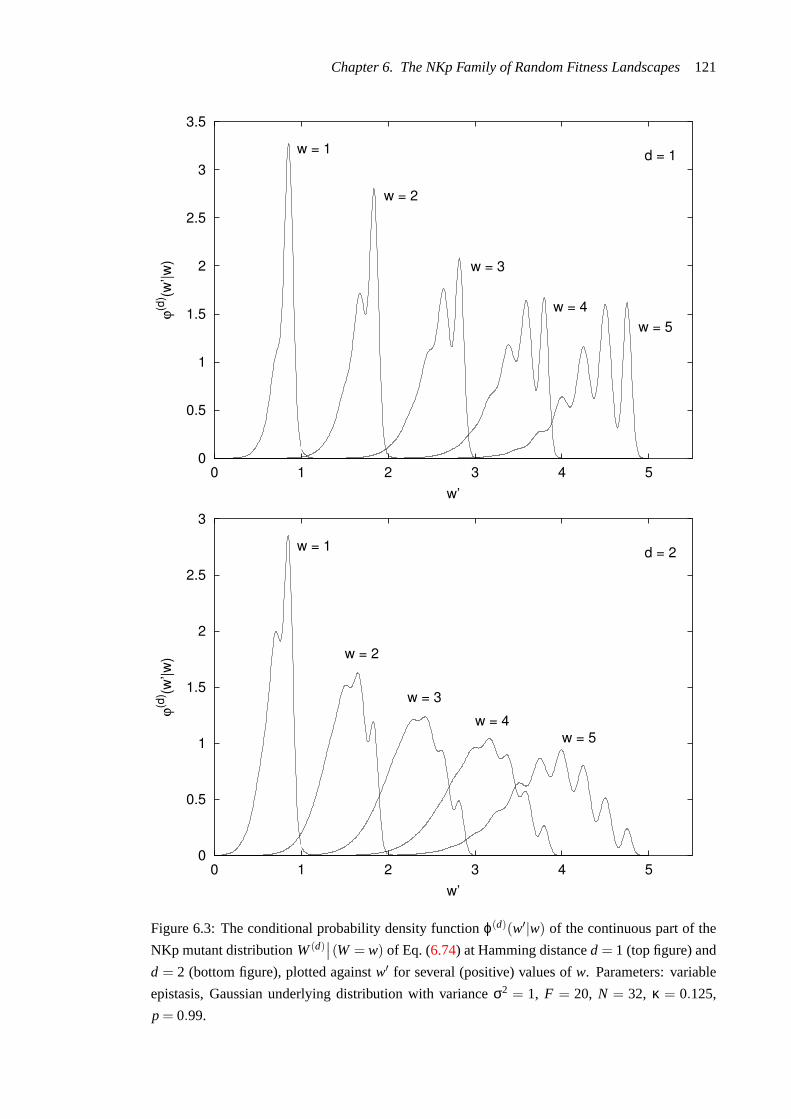
Chapter 6. The NKp Family of Random Fitness Landscapes121
0
0.5
1
1.5
2
2.5
3
3.5
0 1 2 3 4 5
ϕ(d) (w
’|w)
w’
w = 1
w = 2
w = 3
w = 4w = 5
d = 1
0
0.5
1
1.5
2
2.5
3
0 1 2 3 4 5
ϕ(d) (w
’|w)
w’
w = 1
w = 2
w = 3w = 4
w = 5
d = 2
Figure 6.3: The conditional probability density functionϕ(d)(w′|w) of the continuous part of the
NKp mutant distributionW(d)∣∣(W = w) of Eq. (6.74) at Hamming distanced = 1 (top figure) and
d = 2 (bottom figure), plotted againstw′ for several (positive) values ofw. Parameters: variable
epistasis, Gaussian underlying distribution with varianceσ2 = 1, F = 20, N = 32, κ = 0.125,
p = 0.99.

Chapter 6. The NKp Family of Random Fitness Landscapes122
is theHeaviside(step) distribution function and:
Ψ(w) =1√2π
Z ∞
wexp
(−1
2u2)
du (6.78)
is thecomplementary error function(Gaussian tail), defined byΨ(w)= P(Y > w) for Y∼N(0, 1).Note that the neutral termν(d|w) D(w) does not, of course, contribute to evolvability. Forw = 0
it is clear (by symmetry) that:
E (d |0) =12− 1
2ν(d|0) (6.79)
i.e. given that a mutation of a fitness zero sequence is not neutral, it has an equal chance of
being fitness-increasing or fitness-decreasing. Fig.6.4plotsE (d |w) againstd, w over a range of
(non-negative)w values (see also (Smith et al., 2001;Smith, Husbands, et al., 2002)).
The presence of the Gaussian tail in the expression for evolvability indicates adecayof the or-
der ofe−kw2/w for somek of evolvability against fitness. This rapid decay suggests that NKp land-
scapes will behard to optimise (Section6.4.4) - as we move up the landscape fitness-increasing
mutations quickly become difficult to find. This may be compared with the (approximately)linear
evolvability decay (Section5.4.1) of the Royal Road landscapes of the previous Chapter, which
are consequently far easier to optimise (Section5.4.2).
Optimal mutation rates
It is evident that for a given fitnessw there must be anoptimalmutation rate (cf. Section2.3.4);
that is, ad = d∗(w) which maximisesE (d |w), the probability that mutation finds a higher fitness
sequence (this may be seen clearly in Fig.6.4). Note thatd only enters Eq. (6.76) via the auto-
correlation termρ(d). Now ρ(d) = (1−κ)d for the variable epistasis model and≈ (1−κ)d for
the fixed model for smalld, κ, so thatρ′(d) = (1− κ)d log(1−κ). For fixedw we can thus
differentiateE (d |w) with respect tod, set the result to zero and solve (at least numerically) for
an optimald. This may be extended to other mutation modes; for instance, for Poisson mutation
we may calculate an optimum per-sequence mutation rate ¯u∗(w).From Eq. (6.79) we see that for the particular casew = 0 this amounts to minimising the
probability that ad-bit mutation isneutral; but this implies settingd to its maximum value ofL: if
we have a sequence of fitness zero, we should flipeverybit! This may seem peculiar, until we note
the essential difference from e.g. the situation in the previous Chapter. There we were dealing
with a single fitness landscapes. Here we are dealing withensembleevolvability statistics, which
implies that in collating the statistics through sampling we sample a different landscape on each
trial. Our conclusion - that we should flip every bit - is correct. It is, however, evidently less than
useful, as it does not tell us what to do if our mutant doesnot find an innovation and we have to
mutate again; Eq. (6.79) then only tells us what we might expect for adifferent landscape! (We
certainly do not, for instance, wish to flip allL loci back to their original alleles...)
This is, in a sense, an inherent problem with ensemble statistics, at least insofar as they don’t
“self-average” (as is evidently the case for theE (d |w) of Eq. (6.76)). A more meaningful statistic
- in the current case of evolvability - might be the probability that of, say,k uniform randomly
selectedd-flip mutants ofk sequences of given fitnesson the same NKp landscape, (at least) one
of them be fitness-increasing. We might then attempt to find a mutation rate so as to minimise the
expected time to discovery of such beneficial mutations. This approach, while perhaps not entirely
intractable to analysis, would certainly involve far more work... we do not pursue it here.

Chapter 6. The NKp Family of Random Fitness Landscapes123
0.2
0.40.6
0.81
w0 4 8 12 16 20 24 28 32
d
0
0.02
0.04
0.06
0.08
0.1
E(d|w)
0.002
0.0040.006
0.0080.01
w0 4 8 12 16 20 24 28 32
d
0
0.02
0.04
0.06
0.08
0.1
E(d|w)
Figure 6.4: The NKp evolvability statisticE (d |w) of Eq. (6.76) and Eq. (6.79) plotted against
d and 0≤ w≤ 1 (top figure) and 0≤ w≤ 0.01 (bottom figure). Parameters: variable epistasis,
Gaussian underlying distribution with varianceσ2 = 1, F = 20,N = 32,κ = 0.125,p = 0.99.

Chapter 6. The NKp Family of Random Fitness Landscapes124
Nonetheless, the mutation rated∗(w) which maximisesE (d |w) might still be useful as a
“heuristic” for setting a mutation rate in the circumstance that we are attempting to optimise on an
(unknown) member of an NKp family of landscapes. We shall test this hypothesis below.
The “1/e rule” revisited
Another possibility was raised in the conclusion to the previous Chapter: we might assume that
NKp landscapes are “locallyε-correlated” and use an on-the-fly neutrality estimate plus our 1/e
rule to set a mutation rate. We may justify this procedure further by the following argument, which
suggests that the 1/e rule may apply in more general circumstances thanε-correlated landscapes.
Inman Harvey10 has espoused the idea that, in the presence of neutralityand correlation, in order
to maximise the probability of finding a portal to a higher-fitness network by mutation we should
mutate “just enough” to get off the current network but (due to the assumption of correlation) at
the same time to stay as near as possible to the current network. We already know from Prop.2.3.1
that we should use constant mutation - i.e. flip a fixed number of bits. However, without detailed
knowledge of the local network topology it would not seem possible to calculate what the optimal
ratemight be. As a crude approximation let us suppose that neutral networks in our landscape are
(at least locally) “block-like”: suppose specifically that in the locality of our sequence - i.e. within
small Hamming distances - there aren “neutral loci” andL−n “non-neutral loci”, so that locally
ν = nL . Then if we flip exactlyd (arbitrary) loci, the probability thatk of these loci arenon-neutral
andd−k are neutral is given by:(L−n
k
)(n
d−k
)/(Ld
)≈(
dk
)νd−k(1−ν)k (6.80)
where the approximation holds ford n - a reasonable assumption if neutrality is high and, as
we are in any case assuming, the “block-like” approximation holds for small Hamming distances.
Now in order to “get off the network” but remain “as close as possible” to it, we want to choosed
so as to maximise the probability thatk = 1. This is tantamount to choosingd so as to maximise
dνd−1. As in Prop.5.2.1of the previous Chapter we find that the optimal rated is approximated
by the nearest integer to− 1logν which implies the 1/e rule for observed neutrality. For Poisson
mutation we may check that the optimal (per-sequence) rate ¯u is given, again as in Chapter 5, by1
1−ν , which again yields a 1/e rule for observed neutrality.
We remark that for NKp landscapes with reasonably high neutrality and correlation, investiga-
tions by the author (not shown) suggest that neutral networks are in fact quite “block-like” locally.
To test the viability of 1/e Neutral Mutation Rule mutation we calculated, forw in a given range,
the optimum mutation ratesd∗(w) (resp.u∗(w)) for fixed (resp. Poisson) mutation from Eq. (6.76).
Then, for eachw in the range, we calculated the (1-flip) neutralityν = ν(1|w) from Eq. (6.61) and
the mutation ratesdest=− 1logν (resp.uest=
11−ν ) predicted by the 1/e rule for (1-flip) neutrality
ν. These estimated optimum rates were then compared with the “true” optimum ratesd∗(w) (resp.
u∗(w)). Except at very small fitness (in which case discovering innovations is comparatively sim-
ple and mutation rates non-critical) the estimated optimum rates calculated in this fashion proved
to track the true optimum rates surprisingly well. Fig.6.5plots a sample calculation for constant
and Poisson mutation. As in the previous Chapter there is, due to the diminishing of neutrality with
increasing fitness, a tendency slightly to overestimate optimum mutation rates, particularly at low
10Personal communication.

Chapter 6. The NKp Family of Random Fitness Landscapes125
fitness. With the caveat regarding ensemble statistics, these results are encouraging and suggest
that the 1/e rule may be at the very least a useful heuristic for estimating optimal mutation rates
on NKp(-like) landscapes. This proposition will be further tested below where we runadaptive
netcrawlerson NKp landscapes.
6.4 Landscape Modelling with NKp Landscapes
The“typical” scenario for the type of real-world artificial evolutionary optimisation problem we
wish to address exhibits the following features:
• large search space - i.e. long sequence lengths
• substantial neutrality, especially at low fitness
• reasonable degree of correlation
• “most” sequences have low/zero fitness
• higher fitness networks “percolate” to some degree - i.e. are accessible via a few mutationsfrom an arbitrary sequence
It is this type of landscape that we hope to model using NKp landscapes. In simulation, for the
purposes of gathering statistics (where substantial sampling is likely to be necessary) there will
inevitably be a trade-off between realism and time/space/processing constraints. After some ex-
perimentation we arrived at the following NKp parameters which (hopefully) capture the features
itemised above:
F = 40
N = 64
κ = 0.1875 (variable epistasis)
p = 0.999
These parameters settings, which we shall refer to as defining ourlong sequence length baseline
landscapes, yield the following statistics:
• sequence space size= 264≈ 1.84×10¹⁹ sequences
• ≈ 96.08% of landscape is zero fitness
• neutrality at zero fitness≈ 0.99
• (auto-)correlation at Hamming distance 1 is 0.8125
with network percolation to be investigated.
Now the large sequence space and high degree of “lethality” presents a sampling problem: we
are (for reasons already explained) interested in fitness-dependent statistics, but uniform sampling
introduces a heavy bias towards lethal/low fitness sequences. It is non-trivial even tofind higher
fitness sequences (if it weren’t we would hardly attempt to model a difficult optimisation problem
using NKp landscapes!) so that ultimately we must use a search technique to locate higher-fitness
sequences. But this will inevitably introduce (probably unknown) biases into our sampling. There

Chapter 6. The NKp Family of Random Fitness Landscapes126
0
1
2
3
4
5
6
7
0 0.2 0.4 0.6 0.8 1 1.2 1.4
(per
-seq
uenc
e) m
utat
ion
rate
w (fitness)
(constant mutation)
d*(w) = optimumdest(w) = estimated
0
1
2
3
4
5
6
7
0 0.2 0.4 0.6 0.8 1 1.2 1.4
(per
-seq
uenc
e) m
utat
ion
rate
w (fitness)
(Poisson mutation)
u*(w) = optimumuest(w) = estimated
Figure 6.5: Optimum mutation rates calculated from the evolvability statistic (Eq.6.76) and esti-
mated optimum rates based on neutrality (Eq.6.61) and the 1/e Neutral Mutation Rule (see text)
for constant (top figure) and Poisson (bottom figure) mutation modes. Parameters: variable epista-
sis, Gaussian underlying distribution with varianceσ2 = 1, F = 20,N = 32,κ = 0.125,p = 0.99.

Chapter 6. The NKp Family of Random Fitness Landscapes127
would not seem to be a way around this conundrum. The best we can perhaps do, is to check our
sample statistics againstsmall (i.e. short sequence length) landscapes, where uniform sampling
is feasible by exhaustive search; if our optimisation-based sampling technique produces statistics
that tally well with those produced by true uniform sampling at short sequence lengths, we then
hope that our methods scale up benignly to longer sequence lengths... Such checks were carried
out as far as possible on all statistical analyses presented in the following sub-Sections.
Anticipating some results below on optimising on NKp landscapes, the technique we chose to
sample long sequence length landscapes wassimulated annealing(Chapter3, Example3.2.7) with
constant mutation at the theoretical (fitness-dependent) optimal rate based on Eq. (6.76). The an-
nealing schedule was as follows11: temperatureT(τ) decays exponentially with time. Temperature
decay rate and “Boltzmann’s constant”k were controlled by two (constant) parameters:
1. a fitness decrement∆w defined by the property that at the start of a run (i.e.τ = 0) a drop infitness of size∆w is accepted with probability12
2. a “half-life” τ1/2 such that the temperature halves inτ1/2 time steps
Exhaustive (and exhausting!) experimentation revealed that, for long sequence length baseline
landscapes, best results (over a range of time scales) were achieved with parameter settings:
∆w = 0.01 andτ1/2 = 0.2× (run time) (cf. Eq.6.83). It was found by lengthy simulations that the
mean maximum fitness achieved by this technique for our baseline landscapes is approximately12
0.2 with a standard deviation of approximately 0.03. Due to the atomicity of the underlying dis-
tribution around zero, statistics for fitness zero networks were generally omitted from optimising
runs and compiled separately.
Of course there are some statistics which, due to the size of the sequence space and of the
neutral networks themselves cannot be estimated by sampling. These include neutral network
connectivity, distribution of network size and of network number. For these statistics the best we
can do is exhaustive sampling of short sequence length landscapes and again hope that (qualitative)
results scale to higher sequence lengths. We chose ourshort sequence length baselinelandscape
parameters to be:
F = 20
N = 16
κ = 0.375 (variable epistasis)
p = 0.99
yielding:
• sequence space size= 216 = 65536 sequences
• ≈ 81.79% of landscape is zero fitness
11We experimented with other (possibly more conventional) annealing schedules, but the exponential cooling schemedescribed here turned out to be the most effective.
12We suspect that this is close to the mean global optimum fitness for the long sequence length baseline family ofNKp landscapes. Runs of up to 1,000,000 evaluations were used to derive these results. For comparison, in a run ofsimilar length,random searchfinds a mean maximum fitness of around 0.1.

Chapter 6. The NKp Family of Random Fitness Landscapes128
• neutrality at zero fitness≈ 0.93
• (auto-)correlation at Hamming distance 1 is 0.625
• network percolation to be investigated
For both long and short sequence length baseline landscapes, the underlying distribution used was
Gaussian with varianceσ2 = 1.
6.4.1 Estimating landscape parameters
A question of interest is the following: suppose we are given an artificial evolution landscape to
optimise and we suspect that it may resemble structurally an NKp landscape with variable epistasis
and Gaussian underlying distribution (cf. the discussion in Chapter1, Section1.1.2). How might
we then go about verifying our suspicion and estimating the landscape parametersF , κ, p andσ2
(with a view, perhaps, to exploiting some of the theoretical results of this Chapter)? Let us first
suppose that the “ground level” of our landscape - the setC0 of sequences with zero contributing
features - is indeed at fitness zero. This set may be easily established for our unknown landscape
by evaluating fitness for a sample of random sequences, the overwhelming majority of which will
(by assumption that we can indeed model our landscape as an NKp landscape) yield the same
“poor” fitness value. If this value isnot zero, we may either have to offset fitness by an appro-
priate amount or, if fitness is always positive and we suspect that the fitness of features aggregate
multiplicatively, we might redefine fitness to its logarithm. Next we might explore thecorrelation
properties of our landscape. Thus we begin to optimise (using, perhaps, a simulated annealer as
described above) and gather statistics on the mean fitness ofd-bit mutants of sequences of a given
fitness. If mean mutant fitness appeared to satisfy thelinear correlationproperty (Prop.6.3.1)
then we would haveF (d |w) = ρ(d)w. Repeating this process for several values ofd, we could
then check how well the relationρ(d) = (1− κ)d (Eq. 6.9) holds up and estimate the epista-
sis κ. Next we check the neutrality and lethality properties of our landscape. We should have:
ν(d) ≈ exp(−d(1− p2)Fκ
)(Eq. 6.39) andλ(d) = pF (Eq. 6.42) for any d. If these properties
appear to obtain we may use them to estimate neutralityp and number of featuresF . It remains
to estimate the varianceσ2 of the underlying distribution. We may verify from Eq. (6.34) that if,
as in Section6.3.3, the underlying fitness distributionY is defined by1F Y ∼ N
(0, σ2
), then the
fitness variance of an arbitrary sequence is given byvar(W) = F(1− p)σ2. Alternatively, we may
calculate from Eq. (6.75) that the variance of ad-bit mutant of a fitness zero sequence is given by
var(W(d)
∣∣ W = 0)
= F(1− p)(1−ρ(d))σ2. Of course the statistics suggested above to estimate
model parameters areensemblestatistics, but, we hope, may nonetheless yield useful insights into
the structure of our landscape; there is much scope for research in this area.
6.4.2 Notes on NKp computer implementation
Due to the necessarily intensive nature of our statistical sampling, efficiency of implementation
was paramount. An inherent problem regarding computer implementation of NK landscapes in
general is storage requirements: for each feature, if there arek influencing loci, the fitness table
for that feature must contain 2k (real) numbers. Ifk is too large, available computer memory
resources may be insufficient and the processing overhead of pseudo-random number generation

Chapter 6. The NKp Family of Random Fitness Landscapes129
required to fill the tables unacceptable. Several schemes to overcome these problems have been
suggested in the literature - see eg. (Altenberg, 1995). One option to reduce storage requirements
is to storeseedsto the random number generator in tables, rather than fitness itself. Fitness is
then calculated “on-the-fly” using the random number generator with the appropriate seed. This
effectively shifts resource limitation problems from storage to processing time.
We addressed this issue with something of a compromise: we did not actually require very high
epistasis for the modelling intended. For consistency with our analysis wedid, however, wish to
use variable-length epistasis, which implies that there could potentially be up toL influencing loci,
with a storage requirement of 2L real values. The practical limit to the number of influencing loci
as regards storage/processing was found to be aboutk = 20, requiring about 64Mb of storage per
table13. However, it may be checked that for theκ andL in our long sequence length baseline
parameter settings, the probability of more than 20 influencing loci is≈ 0.005, which was found
to be acceptably small; we simply rejectedk > 20 when assigning epistasis. This was found to be
statistically insignificant.
For (pseudo-)random number generation - for assignation of epistasis as well as sampling the
underlying distribution for the fitness tables - we used theMersenne Twistergenerator (Matsumoto
& Nishimura, 1998), which combines speed and good statistical properties, as well as having a
very long period. Fitness table values were generated from 64-bit random deviates and stored in
double-precision (64-bit) floating point format14.
As regards neutrality, we have found from past experience on a number of computer plat-
forms that comparing floating-point fitness values in order to determine whether two sequences
are actually of equal fitness - i.e. in the same neutral network - can often beunreliable, due to
floating-point arithmetic rounding error. To avoid this problem, we devised an efficient binary
“phenotype” for NKp landscapes as follows, based on the “Central Property” (Section6.2.2) for
NKp landscapes: for each feature the phenotypes has a string of bits of lengthL+1. The first (low)
bit is set to 1 (resp. 0) according as that feature is contributing (resp. non-contributing). If the
feature is contributing, the remainingL bits are filled sequentially (low to high) with the (binary)
allele at each of the(≤ L) loci (again read low to high on the sequence bit-string) influencing the
given feature and then padded with zeroes; if the feature is non-contributing, the remainingL bits
are filled with zeroes. These phenotypes may be safely compared (bit-wise) to decide whether two
sequences are of equal fitness.
6.4.3 Neutral Network Statistics
We now turn our attention to some statistical properties of the neutral networks on NKp land-
scapes, namelyconnectivity, network size/numberandpercolation/innovation. All but network
size are not easily amenable to mathematical analysis. Connectivity and network size/number15
distribution, furthermore require exhaustive sampling; we use our short sequence length baseline
parameters to compile exhaustive-sampling statistics. Percolation/innovation statistics may be col-
13Based on 64 bits per double-precision floating-point number.14This is arguably ”overkill” as regards our statistical needs. For instance, even with 32 bit precision, the probability
that two sequences evaluate to the same fitness when different fitness table entries are indexed - thus violating the“Central Property” - would be< 2−32.
15Investigations into network connectivity and number distribution are at the time of writing still preliminary. Wehope to present more detailed results at a later stage.

Chapter 6. The NKp Family of Random Fitness Landscapes130
lated by the optimisation-based method described above; we use our long sequence length baseline
parameters.
Distribution of network size
To estimate the fitness dependence of neutral network size, a little thought convinces that, since all
sequences on a neutral network share the same non-zero fitness contributions, the distribution of
sizeof neutral networks for NKp landscapes depends just on the number of contributing features
rather than on fitness itself. We thus (for the variable epistasis case) estimate the expected size of
the neutral network of an arbitrary sequence given that that sequence hasc contributing features.
Consider a sequence chosen uniformly at random from an arbitrary NKp landscape. Let the
random variableC be the number of contributing features of our sequence and let the (jointly
distributed) random variableSbe the size of the (maximal) neutral network of which our chosen
sequence is a member. We wish to calculateE(S | C = c).We condition on the r.v.R representing the number of loci whichdo not influence anyof thec
contributing features of our sequence: givenR= r, it is clear that altering the allele at any locus
other than theser cannot be neutral, so that the size of our neutral network is consequently≤ 2r .
The probabilityP(R= r) that there arer such loci is easily seen to be(L
r
)ar(1− a)L−r where
a = (1−κ)c. Now the number of neutral mutants of our sequence among the 2r sequences that
may be formed by altering ther loci is precisely the number of sequences with zero contributing
features that we would expect to find on an NKp landscape with the same epistasis and neutrality
parameters, but withF−c features and sequence lengthr. From Eq. (6.27) the probability that an
arbitrary sequence chosen from an arbitrary NKp landscape withF features is fitness zero (i.e. has
zero contributing features) is justpF . Theexpectednumber of sequences of fitness zero, where
sequence length isr and there areF−c features, may consequently be approximated aspF−c ·2r
(this will not be exact, since the probabilities that different sequences on thesamelandscape are
fitness zero are not independent). Thus we derive, summing conditionally overr:
E(S | C = c)≈ pF−c [1+(1−κ)c]L (6.81)
We may now use Eq. (6.59) to approximate the fitness-dependence of expected network size: ifW
is the fitness of an arbitrary sequence, then:
E(S | W = w)≈F
∑c=0
E(S | C = c)γ(c|w) (6.82)
Exhaustive sampling on short sequence length landscapes (L ≤ 20) indicated that the approxima-
tion is reasonably accurate (Fig.6.6). Fig. 6.7 plots fitness-dependence of (estimated) mean net-
work sizeE(S | W = w) from Eq. (6.81) and (6.82) against neutralityp (top figure) and epistasis
κ (bottom figure) for a range of fitness valuesw. Except at very low fitness, we see that for small to
medium fitness values network size drops off quite slowly with fitness. Beyond a (roughly defined)
critical fitness (the “ridge” in the size/fitness plots) network size attenuates roughly exponentially
with increasing fitness. For given fitness, network size increases approximately exponentially with
increasing neutrality. Scaling of network size with epistasis is somewhat more complex. At low-
medium fitness, network size increase roughly exponentially with decreasing epistasis. Beyond

Chapter 6. The NKp Family of Random Fitness Landscapes131
0
1000
2000
3000
4000
5000
6000
0 0.02 0.04 0.06 0.08 0.1 0.12 0.14 0.16 0.18 0.2
netw
ork
size
fitness
Figure 6.6: Exhaustively sampled NKp mean neutral network size for short sequence length base-
line parameters (variable epistasis, Gaussian underlying distribution with varianceσ2 = 1,F = 20,
N = 16, κ = 0.375, p = 0.99) plotted against fitness. Number of landscapes sampled= 10,000.
Error bars indicate 1 standard deviation (note large variance). The dashed line is the analytic
(estimated) valueE(S | W = w) of Eq. (6.81) and (6.82).

Chapter 6. The NKp Family of Random Fitness Landscapes132
E(S | W = w)
-1-0.5
0 0.5
1w 0.9 0.92
0.94 0.96
0.98 1
p 1000
10000
100000
1e+06
1e+07
1e+08
1e+09
E(S | W = w)
-1-0.5
0 0.5
1
w
0 0.2
0.4 0.6
0.8 1
κ 0.1
1 10
100 1000
10000 100000 1e+06 1e+07 1e+08 1e+09 1e+10
Figure 6.7: Fitness-dependence of (estimated) mean neutral network sizeE(S | W = w) (note log
scale) for NKp landscapes plotted against neutrality (top figure) and epistasis (bottom figure) for a
range ofw values. Parameters: variable epistasis, Gaussian underlying distribution with variance
σ2 = 1, F = 20,N = 32,κ = 0.125 (top figure),p = 0.99 (bottom figure).

Chapter 6. The NKp Family of Random Fitness Landscapes133
the critical fitness “ridge”, network size increases at a roughly exponential-exponential rate with
decreasing epistasis16.
Fitness distribution of number of networks (preliminary results)
We exhaustively sampled short sequence length baseline landscapes to identify neutral networks,
binning them according to fitness (we thus approximate the “density” of networks vs. fitness).
Results of one such experiment are illustrated in Fig.6.8(Fig. 6.8). Further experimentation with
0
2
4
6
8
10
12
14
16
0 0.02 0.04 0.06 0.08 0.1 0.12 0.14 0.16 0.18 0.2
num
ber o
f net
work
s
fitness
Figure 6.8: Exhaustively sampled NKp mean number of networks (binned vs. fitness) for short
sequence length baseline parameters (variable epistasis, Gaussian underlying distribution with
varianceσ2 = 1, F = 20,N = 16,κ = 0.375, p = 0.99). Number of landscapes sampled= 1000,
error bars indicate 1 standard deviation. Mean total number of networks per landscape was≈78.3±44.1.
different parameter values (not illustrated) suggested the following:
• Number of networks per fitness band drops off with increasing fitness; the attenuation isapproximately linear for small fitness values
• Number of networks increases with decreasing neutralityp
• Number of networks increases with increasing number of featuresF
• Number of networks increases with increasing epistasisκ16See also (Barnett, 1998) for the (somewhat different) scaling of network size for the fixed-epistasis, uniform fitness
distribution case.

Chapter 6. The NKp Family of Random Fitness Landscapes134
Further research is required to elucidate the relationship between number of networks, network
size and network fitness.
Network connectivity (preliminary results)
We partitioned short sequence length baseline landscapes into maximal neutral networks (by ex-
haustive sampling) and then decomposed the maximal networks into connected components with
respect to the Hamming graph structure (i.e. 1-bit mutation). It was found thatdisconnected net-
works were rare: as an example, for one experiment, out of a sample of 10,000 landscapes - for
which 78,299 (maximal) neutral networks were found - only 117 (≈ 0.15%) of the neutral net-
works were found to be disconnected. Further research is required to elucidate the relationship
between network connectivity, size and fitness.
Percolation and Innovation
Simulated annealing as outlined previously was used to collate percolation/innovation statistics
(Section2.2.6) for our long sequence length baseline landscapes. As suggested our sampling
technique was also applied to the short sequence length baseline landscapes and results compared
with equivalent statistics obtained by exhaustive sampling. Results were in good agreement so
that we may hope that sampling bias does not distort results significantly.
The technique was applied as follows: for each landscape of the family sampled, a simulated
annealing run was performed. Each time the simulated annealer discovered a higher fitness net-
work (i.e. a new best-so-far fitness of the current simulated annealing run) a blind ant neutral walk
(Example3.2.5, Section4.1) of a given number of steps was performed on that network using the
extant mutation mode/rate17. A blind ant neutral walk spends asymptotically equal amounts of
time at every sequence of a (connected) network (Section4.1.1) and would thus be expected to
sample the neutral network approximately uniformly. At each sequence along the walk a mutant
was created - again according to the extant mutation mode/rate - and its neutral network collated.
The networks encountered were then used to compile the percolation index (Eq.2.49) and cumu-
lative innovation statistics for the current network. Results were binned according to fitness and
means and variances of the (binned) samples calculated. As mentioned previously, fitness zero
statistics are quoted separately -the “zero bin” doesnot include fitness zero statistics!We remark
that percolation statistics thus compiled appeared to be very robust with respect to thelengthof
the neutral walks.
Fig. 6.9 and Fig.6.10demonstrate the fitness-dependence of effective number of accessible
networks and cumulative innovations for constant 1-bit and 4-bit mutation respectively, for a sam-
ple of 1,000 long sequence length baseline landscapes over neutral walks of 10,000 steps. Results
support the following (somewhat counter-intuitive) interpretation:
• As we move higher up the landscape in fitness, neutral networks percolate more (in thesense that they have more accessible neighbouring networks) despite the fact that, as wehave already seen, they decrease in size. Thus, although we start a neutral walk seeing new(i.e. previously unseen) neighbouring networks at a higher rate, we “run out” of accessiblenetworks sooner than for lower fitness networks.
17The mutation rate used by the simulated annealer was not necessarily the same as that used to compile networkstatistics.

Chapter 6. The NKp Family of Random Fitness Landscapes135
1
2
3
4
5
6
7
8
9
10
0 0.02 0.04 0.06 0.08 0.1 0.12 0.14 0.16 0.18 0.2
effe
ctive
acc
essib
le n
etwo
rks
fitness
0
5
10
15
20
25
30
35
40
0 2000 4000 6000 8000 10000
cum
ulat
ive in
nova
tions
steps
w = 0.00 - 0.02w = 0.02 - 0.04w = 0.04 - 0.06w = 0.06 - 0.08w = 0.08 - 0.10w = 0.10 - 0.12w = 0.12 - 0.14w = 0.14 - 0.16w = 0.16 - 0.18w = 0.18 - 0.20
0
4
8
12
0 100
Figure 6.9:Top: Mean (sampled) effective accessible networks (percolation index) for constant
1-bit mutation plotted against network fitness. Error bars denote one standard deviation.Bottom:
Cumulative innovations plotted against neutral walk steps. Inset shows first 100 steps of walk.
Parameters: variable epistasis, Gaussian underlying distribution with varianceσ2 = 1, F = 40,
N = 64,κ = 0.1875,p = 0.999. Sample size = 1,000 landscapes, neutral walk steps = 10,000.

Chapter 6. The NKp Family of Random Fitness Landscapes136
0
5
10
15
20
25
30
0 0.02 0.04 0.06 0.08 0.1 0.12 0.14 0.16 0.18 0.2
effe
ctive
acc
essib
le n
etwo
rks
fitness
0
10
20
30
40
50
60
70
80
90
100
0 2000 4000 6000 8000 10000
cum
ulat
ive in
nova
tions
steps
w = 0.00 - 0.02w = 0.02 - 0.04w = 0.04 - 0.06w = 0.06 - 0.08w = 0.08 - 0.10w = 0.10 - 0.12w = 0.12 - 0.14w = 0.14 - 0.16w = 0.16 - 0.18w = 0.18 - 0.20
0
5
10
15
20
0 100
Figure 6.10:Top: Mean (sampled) effective accessible networks (percolation index) for constant
4-bit mutation plotted against network fitness. Error bars denote one standard deviation.Bottom:
Cumulative innovations plotted against neutral walk steps. Inset shows first 100 steps of walk.
Parameters: variable epistasis, Gaussian underlying distribution with varianceσ2 = 1, F = 40,
N = 64,κ = 0.1875,p = 0.999. Sample size = 1,000 landscapes, neutral walk steps = 10,000.

Chapter 6. The NKp Family of Random Fitness Landscapes137
Now we also know that networksneutralitydecreases as we ascend the landscape. We compiled
neutrally adjustedpercolation statistics for the same parameter values (Eq.2.53, Section2.2.6);
i.e. neutral mutations are omitted from the entropy calculation. Results showed surprisingly little
difference from the comparable un-adjusted statistics. We could interpret this as follows:
• Lower percolation at lower fitnesscannotbe ascribed simply to higher network neutrality.
As might be expected, network percolation also increases with increasing mutation rate. We also
compiled statistics for Poisson mutation. Results (omitted) were similar to those for constant
mutation.
6.4.4 Hill-climbing on NKp Landscapes
A thorough (empirical) comparative investigation of evolutionary optimisation performance on
NKp landscapes - perhaps along the lines of Section5.4.2for Royal Road landscapes - is beyond
the scope of this study. We did, however, conduct some experiments withstochastic hill-climbers
(Chapter3, Example3.2.5) to test some of our theoretically motivated assertions regarding opti-
mal mutation mode/rate, adaptive netcrawling and the 1/e Neutral Mutation Rule. The artificial
evolution scenario we attempt to model is the following: we arenot necessarily attempting to
locate a global optimum fitness; rather, much as in the previous Chapter, we take atime-critical
perspective (cf. Section3.5) and suppose that there is a maximum acceptable number of fitness
evaluationsT∗, say, beyond which we will terminate any optimisation run. The object of optimi-
sation is then to achieve the highest possible fitness within theT∗ available fitness evaluations.
Our performance measure is the expected best-so-far fitness achieved inT∗ evaluations.
We choseT∗ = 10,000 evaluations as our benchmark for evolutionary optimisation. At this
number of evaluations, the best achieved performances (see below) were in the region of fitness
= 1.8, which we think to be (see footnote above) approximately 90% of the mean global optimum
fitness for the landscape family; we consider this to be a credible scenario for a real-world optimi-
sation problem, in the sense that 90% of maximum achievable fitness may be a reasonably realistic
“acceptable” figure for fitness. The hill-climbers tested were a netcrawler (NCR) and stochastic
annealing with the “multiplicative” schedule/parameters described in the introduction to this Sec-
tion (SAM). These were each run with constant (CON) and Poisson (POI) mutation at both a fixed,
“hand-optimised” rate (FIX) or at the theoretical optimal rate (OPT) - i.e. the (fitness-dependent)
rate which maximises the evolvabilityE (U |w) as calculated from Eq. (6.76). The netcrawler was
also run in an adaptive mode (ADP) as described in Section5.4.2for Royal Road landscapes18, so
as to implement the 1/e Neutral Mutation Rule (Prop.5.3.1). Random search results (RSH) are
18Note that a comparable adaptive mutation rate scheme for a simulated annealer would not be practicable, as theannealer will not generally linger long enough on a network to estimate its neutrality reliably, particularly at highertemperatures.

Chapter 6. The NKp Family of Random Fitness Landscapes138
included for comparison. Hill-climber parameters were as follows:
NCR CON FIX u = 4
NCR POI FIX u = 4.0
NCR CON ADP tlag = 350
NCR POI ADP tlag = 500
SAM CON FIX u = 2 ∆w = 0.006 τ1/2 = 0.40×T∗
SAM POI FIX u = 3.25 ∆w = 0.007 τ1/2 = 0.35×T∗
SAM CON OPT ∆w = 0.010 τ1/2 = 0.20×T∗
SAM POI OPT ∆w = 0.007 τ1/2 = 0.25×T∗
(6.83)
(note that NCR CON OPT and NCR POI OPT do not have any tunable parameters). We make the
following observations on results:
1. NKp landscapes arehard to optimise (certainly compared, eg., with Royal Road landscapes;contrast Fig.6.11with the comparable Fig.5.8of the previous Chapter and note that in theformer the time scale islogarithmic). This is consonant with our theoretical results onevolvability(Section6.3.3), in particular our observations on the decay of evolvability withincreasing fitness.
2. Constant (n-bit) mutation (CON) generally outperforms Poisson mutation (POI), as cor-rectly predicted by Prop.2.3.1. For constant mutation, furthermore, since (per-sequence)mutation rates are generally low ( ¯u≈ 1−3 for the theoretical optimal (OPT) and adaptive(ADP) mutation regimes at medium-to-high fitness) portals are being discovered close to thecurrent network. This implies that optimisation tends to proceed via the crossing ofentropyrather thanfitnessbarriers as described in Section3.4.1. Even for quite high fitness, neutralnetwork volumes are large (as may be calculated from Eq.6.82) , but portals to still highernetworks become increasingly sparse and difficult to find. However...
3. ...the simulated annealers generally outperform the netcrawlers19. This suggests that thereare indeed fitness barriers separating thehighestneutral networks fromlocally optimalnet-works, which the annealers, with their capacity to “back down” from a local optimum, areable to escape20 (note, however, that towards the end of a run, as the annealing tempera-ture approaches zero, the process increasingly - as remarked in Example3.2.7- resemblesa netcrawler). The behaviour of simulated annealers seems to suggest a “global” structureconsistent with observations on local optima on (non-neutral) NK landscapes, as reportedeg. in (Kauffman, 1993).
4. Theoretical optimal mutation rates (OPT) - which we recall are based on theensemblestatis-tic E (U |w) - generally outperform fixed mutation rates (FIX). This suggests that in theparameter regime of the experiment ensemble statistics may be useful, although...
5. ...adaptive mutation rates (ADP) outperform theoretical ensemble optimal rates (OPT) forthe netcrawler. Since setting a “true” optimal mutation rate on a per-network basis would beexpected to outperform the “per-fitness” ensemble rate (OPT), this provides good evidencefor the efficacy of the 1/eNeutral Mutation Rule as a heuristic for setting mutation rates.
19In fact, in our preliminary investigations, simulated annealing outperformed every GA tested, both with and withoutrecombination.
20This conclusion is further supported by results of the author (unpublished) onmultiple independent netcrawlerson NKp landscapes: over some time scales and population sizes, multiple netcrawlers (with random start) outperformsingle netcrawlers. Analysis reveals that this is because the multiple netcrawlers may “hedge their bets” - while mostwill generally start in the “basin of attraction” of a locally sub-optimal network, a few tend to strike it lucky and startfrom the basin of attraction of a globally optimal, or at least high fitness, network.

Chapter 6. The NKp Family of Random Fitness Landscapes139
0
0.02
0.04
0.06
0.08
0.1
0.12
0.14
0.16
1 10 100 1000 10000
mea
n fit
ness
time (evaluations)
RSHNCR CON FIXNCR POI FIX
NCR CON OPTNCR POI OPT
NCR CON ADPNCR POI ADPSAM CON FIXSAM POI FIX
SAM CON OPTSAM POI OPT
0.06
0.07
0.08
0.09
0.1
0.11
0.12
0.13
0.14
0.15
SAMCONOPT
SAMCONFIX
SAMPOIOPT
SAMPOIFIX
NCRCONADP
NCRPOIADP
NCRCONOPT
NCRPOIOPT
NCRPOIFIX
NCRCONFIX
RSH
mea
n fit
ness
Figure 6.11:Top: Optimised hill-climber performance on long sequence length baseline NKp
landscapes (variable epistasis, Gaussian underlying distribution with varianceσ2 = 1, F = 40,
N = 64,κ = 0.1875,p= 0.999): mean best-so-far fitness (sample size 10,000 runs) plotted against
time in fitness evaluations. See text for key and parameters. The bottom figure shows a histogram
of mean best-so-far fitness at the end of each run, ranked by performance.

Chapter 6. The NKp Family of Random Fitness Landscapes140
We see in particular that the long sequence length, variable epistasis, Gaussian NKp landscapes of
our experiment differ significantly from theε-correlated landscapes of the previous Chapter. From
a practical point of view we also note that the adaptive netcrawlers have a single parameter (the
“window” time-lag tlag) which has a very large “sweet spot”, making them particularly simple to
tune, almost independently of time-scale (cf. Chapter5). Simulated annealing parameters were
also comparatively easy to tune, although there was some dependence on run length.

Chapter 7
Recombination
We have previously in this thesis, counter to orthodoxy, expressly rejected recombination as an
effective mechanism in evolutionary optimisation. In this Chapter we present some justification
for this prejudice; we discuss three reasons why recombination may be ineffective or actually
counter-productive. In brief, they are:
• Failure of the Building Block Hypothesis
• Genetic drift (“convergence”) and hitch-hiking
• Error thresholds and the “bi-stability barrier”
The Building Block Hypothesis may be regarded asstructural by nature; it is deeply bound to
the coding of an artificial evolution problem. Although it has been quite extensively criticised
in the literature (Grefenstette & Baker, 1989; Altenberg, 1994) it nevertheless still appears to
underpin (consciously or not) much of the thinking in the GA community; to this author’s mind,
this may be ascribed, to some extent, to over-reliance on unrealistic model fitness landscapes.
The related phenomena of genetic drift and hitch-hiking arise from finite-population stochastic
population sampling. Genetic drift - under itsnom-de-guerreof “(premature) convergence” - is
widely perceived as a serious problem for genetic algorithms and generates a wealth of literature
(although surprisingly little serious analysis). Its partner in crime, hitch-hiking, although not
as widely appreciated as it should be, has been identified and quite thoroughly analysed in the
literature (Forrest & Mitchell, 1993; Mitchell et al., 1992). The third phenomenon - the main
subject of this Chapter - has not, to the author’s knowledge, been identified previously. It makes its
presence felt in the (deterministic)infinite population limitbut is exacerbated by finite population
effects.
We do not wish to write-off recombination completely; indeed, GA researchers routinely re-
port improved performance with recombination - although to what extent this may be due to unsuit-
able evolutionary algorithms or poor choice of parameters (in particular mutation rates) remains
moot. It is perhaps worth noting that, while the evolution of sex and recombination remains a
highly active (indeed frequently somewhat overheated) topic in evolutionary genetics, few popula-
tion geneticists would quote similar justification for recombination as the standard GA perspective

Chapter 7. Recombination142
might have it; for whatever reasons recombination evolved in the natural world, those reasons are
unlikely to be those identified as “useful” from the traditional GA perspective.
7.1 The Building Block Hypothesis
Perhaps at the root of the traditional GA perspective on recombination is the so-calledBuilding
Block Hypothesispromoted by John Holland and subsequent researchers (Holland, 1992). This
identifies genetic “building blocks” withschemata- subsets of loci along with specific alleles at
those loci. A genotype is said to “instantiate” a schema1 if the genotype possesses the requisite
alleles at corresponding loci. It is then supposed that the power of GA’s derives principally from
the ability of recombination to assemble short, fitness-enhancing schemata present in different
genotypes in a population into new, fit genotypes. The “building block” schemata are assumed
short in comparison to the genotype sequence length, so that they are not too frequently disrupted
by (say, one- or two-point) crossover (Fig.7.1).
crossover point
Figure 7.1: The Building Block Hypothesis: recombination (here with single-point crossover)
splices two parent genotypes with short, fitness-enhancing schemata, so that both schemata are
present in the offspring genotype.
In the next Section we shall question how effective this mechanism is likely to be with re-
gard to the dynamics of population-based evolutionary algorithms. Here, we ask two perhaps
more fundamental questions:Why should we expect fitness-enhancing schemata to recombine
successfully?and: Why should we expect short, fitness-enhancing schemata to exist at all?To
answer these question we need to examine more carefully what we mean by a “fitness-enhancing”
schema. We might be tempted to describe a schema as fitness-enhancing if sequences instantiating
that schema are fitter “on average”. A schemaξ, say, may be identified with the subset of all those
sequences that instantiate it; i.e. we may considerξ⊂ AL whereAL is the sequence space2. Thus
we might callξ fitness-enhancing if the mean fitness of sequences instantiatingξ is higher than
the mean fitness of an arbitrary sequence; more precisely, if the fitness function for our landscape
is f : AL −→ R we have:1|ξ|∑
x∈ξf (x) >
1|AL| ∑
x∈AL
f (x) (7.1)
1Alternatively, the schema is “present” in the genotype.2Note, though, that not every subset ofAL may be identified with a schema.

Chapter 7. Recombination143
This doesn’t, of course, imply thatf (x) is higher than average forevery x∈ ξ. Nor does it follow
that there will beshort schemata satisfying this condition. Now supposeA⊂ AL is some subset
of sequence space. Then (7.1) doesnot imply that sequences inξ∩A are on average fitter than an
arbitrary sequence drawn fromA. This is due toepistasis: the effect on fitness of a particular allele
at a particular locus may depend on the alleles at other loci. The effect on fitness of a schema is in
this sensecontext-dependent. This observation engenders two major implications:
1. A is the set of sequences represented in an evolving population.We have stressed previously(Section1.1.3), that uniform sampling is likely to be highly unrepresentative of sequencessampled by an evolutionary process; even if a schema is fitness-enhancing “on average” itneed not be fitness-enhancing for sequences in an evolving population.
2. The set A is that defined by another schema.The implication is that even if a schemaenhances fitness on average for arbitrary sequences, it need not enhance fitness for sequencesthat instantiate someotherschema.
The first point might conceivably be remedied by re-defining “fitness-enhancing” to mean “fitter
than average within the context of a (given) population”. The second point seems more diffi-
cult to address; it implies in particular that we cannot assume in general that splicing sequences
instantiating fitness-enhancing schemata will yield above-average fitness sequences.
Of course, there are landscapes where we may readily identify fitness-enhancing (in some
sense of “above average fitness”) schemata which manifestlydo recombine successfully; perhaps
the best-known example would be the Royal Road landscapes (Chapter5), which were designed
specifically with this in mind (Mitchell et al., 1992); here, set blocks may be considered as emi-
nently splice-able building blocks. The above objections do not apply to such landscapes (although
those of the next Section do).
A related problem with the Building Block Hypothesis is that recombination can only assem-
ble disjoint schemata. For the Royal Road landscapes this is not a problem, since the “good” (i.e.
short, fitness-enhancing) schemata are in fact disjoint. In contrast, consider the NKp landscapes
of Chapter6: given some feature, we may may pick out the loci influencing that feature and a
set of alleles for those loci which reference a high-fitness contribution; this yields a candidate
fitness-enhancing schema. We note that for the “random epistasis” models presented in Chap-
ter 6 these schemata are not particularly likely to be short; other epistatic assignment schemes
such as “adjacent neighbourhood” (Kauffman, 1993) might be expected to yield shorter schemata.
But (even for nearest-neighbour models) if we examined these “natural” schemata for anactual
high-fitness sequence, we would be likely to find, particularly at higher epistasis, that theyover-
lap to a large degree and thus could not have been spliced together by crossover. Epistasis in the
NKp model dictates that “good” schemata are not generally good in the context of other “good”
schemata - they frustrate each other. In the terminology of Gavrilets’holey landscapes(Gavrilets
& Gravner, 1997), on an epistatic landscape recombination lands us in the holes. (Altenberg, 1995)
addresses similar concerns. He uses Price’s Covariance and Selection Theorem (Price, 1970) to
derive a version of Holland’s Schema Theorem (Holland, 1992) which goes some way to identi-
fying “good” schemata (with respect to a particular recombination operator - essentially the short,
disjoint schemata for one or two point crossover) and, by incorporating the fitness distribution of

Chapter 7. Recombination144
recombinant offspring into the analysis, quantifies the extent to which a GA is liable to exploit
them successfully:
“[The variant Schema Theorem] ... makes explicit the intuition about how schemaprocessing can provide a GA with good performance, namely: (1) that the recombi-nation operator determines which schemata are being recombined; and (2) that thereneeds to be a correlation between [disjoint] schemata of high fitness and the fitnessdistributions of their recombinant offspring in order for the GA to increase the chanceof sampling fitter individuals.”
We turn next to some real-world artificial evolutionary problems and ask whether we might
expect to find combinable building blocks. Consider the thought experiment (the “Fitness Land-
scaper”) of the introductory Chapter: here the problem to be solved is the design of a software
controller for a robot required to perform, say, a navigational task. The chosen implementation
is a highly recursive neural network, with the connections, weights and timescale parameters en-
coded in a genotype after some “natural” fashion. Now we might expect that the fitness function
is “modular” in the sense that high fitness is conferred by success at various behaviours (“move
towards light”, “turn away from obstacle”, “move in an arc”,etc.). Yet, if we looked for a causal
origin of these behaviours in the neural network - that is, if we attempted to map modularity at
the fitness level to structural modularity in the neural network - we would be likely to fail. The
reason for this is that highly interconnected recursive neural networks are notoriouslysynergistic
in their functioning; every part effects every other (recursively!) and, though a network may in-
deed appear to exhibit discrete behaviours, these behaviours cannot in general be localised, say, to
sub-networks. Now it may be that the genotype→ neural network mapping is “modular”, insofar
as codings for sub-networks may be localised on the genotype; notwithstanding, there will still be
no modularity (or localisation on the genotype) in the mapping from genotype tobehaviour(much
in the same way as fitness contributions in the random epistasis NKp model are not in general lo-
calised on the genotype). Where then are we to find building blocks - fitness-enhancing schemata
- on the genotype? And even if such building blocks existed, network synergy would be likely
to induce extreme context-dependence; we would not expect schemata to recombine successfully,
since (like schemata in the NKp model) they would likely interact to their mutual detriment. Note
that this is not an argument againstcorrelation; neural network landscapes may well be quite
highly correlated (they may also exhibit substantialneutrality). Similar synergistic “phenotypes”,
with concomitant lack of a modular genotype→ fitness mapping, may also be found in other real-
world evolution problems, such as evolving electronic circuits, either on-chip (Thompson, 1996;
Thompson, 1998;Harvey & Thompson, 1996) or in software emulation (Layzell, 2001).
In summary, for a class of real-world optimisation problems - those featuring what we might
termsynergistic phenotypes- we can expect the Building Block Hypothesis to fail because: (1) it
is not clear that suitable building blocks will exist and (2) even if they do exist, they are unlikely
to recombine successfully. We might contrast this with that favourite GA “benchmark”, the Trav-
elling Salesman Problem. Here, (depending on the coding) we may well have a modular genotype
→ fitness mapping;sub-toursmay be fitness-enhancing, may be coded for locally on the genotype
and may well recombine successfully. Note that, nonetheless, TSP landscapes are in general quite
epistatic (Stadler, 1996) (as indeed are Royal Road landscapes) - correlation in itself does not tell
us much about whether preconditions for the Building Block Hypothesis to apply will prevail.

Chapter 7. Recombination145
7.2 Genetic Drift and Hitch-hiking
Genetic drift is the phenomenon whereby stochastic sampling reducesgenetic variationwithin a
finite (fixed size) population. It is most easily apprehended in the absence of mutation - i.e. in the
absence of any mechanism for producing new alleles at a locus. Suppose that at a given locus,
locus i, say, and for a given allelea at locusi there are, say,n sequences in the population with
allelea at locusi. After some numbert of generations, there is afinite probability that, through
failure (via sampling fluctuations) of such sequences to be selected, alln of these sequences have
disappeared from the population; then, since there is no mechanism for regeneratinga at locusi,
allelea is irrevocably lost from the population at locusi. This extends to all alleles at all loci. The
result is that after a sufficient number of generations, there is a finite probability thatall sequences
in the population are copies of a single sequence!- all genetic variation has disappeared.
Crucially, recombination does not affect this conclusion: recombination can only “mix-and-
match” alleles at a given locus. Mutation will counteract this effect by generating new alleles, but
at low mutation rates (and traditionally mutation has been relegated to the status of “background
operator”, implying low mutation rates) there will still be a pronounced loss of variation; the
population will belocalised in sequence space, somewhat like a classicalquasi-species(cf. the
next Section). If, now, a GA relies on recombination as the principal search mechanism, this loss
is catastrophic; recombination requires genetic variation to produce novel sequences. The term
premature convergence(Goldberg, 1989) has been used to describe the effect whereby variation
is lost - and crossover rendered ineffective - before appreciable fitness levels have been achieved.
From the traditional GA perspective, premature convergence has been perceived as perhapsthe
most important problem for the GA designer to overcome, and a remarkably large percentage of
the GA literature is devoted to schemes (crowding, nicheing, fitness sharing and spatial distribution
to name but a few) to reduce the effect.
Hitch-hiking (Mitchell et al., 1992)may be viewed as an exacerbation of the effects of genetic
drift by strong selection: if a new sequence with a strong selective advantage is discovered (by
whatever mechanism), then that sequence (and its neutral offspring) will be strongly selected at
the expense of other sequences. Within a short “takeover” time,all sequences in the population
will be descendants of the new sequence and its neutral variants, with a concomitant drastic loss of
genetic variation. If, in particular, there were useful “building blocks” present in sequencesother
than the new fit sequence, these building blocks will not survive into post-takeover populations.
Conversely, “bad” building blocks in the new fit variant will “hitch-hike” along into future gen-
erations; it is then up to mutation to regenerate variation. Now the takeover time for a sequence
with a strong selective advantage tends to be orders of magnitude shorter than the times between
discovery of fitter variants (Nimwegen et al., 1997). The result is that, even if good, potentially
recombine-able building blocks exist for a GA implementation,good building blocks will rarely
be present simultaneously in different sequences in an evolving population. Recombination thus
is not afforded the opportunity to assemble good building blocks.

Chapter 7. Recombination146
7.3 Recombination, Error Thresholds and the Bi-stability Barrier
In the previous two Sections, we have argued that recombination is likely to be ineffective in
the sense of the Building Block Hypothesis; that is, at discovering fit sequences by recombining
building blocks. But, we should perhaps ask, might not recombination be useful forcreating
good building blocks? We are assuming that our fitness landscapes are to some degree correlated;
this provides a rationale for supposing thatmutationmight discover high-fitness sequences (cf.
Section2.3.4). Might recombination, then, have a similar value? We observe that recombination is
a “contracting” operator; the Hamming distance between a recombinant offspring and either of its
parents is always less than or equal to the Hamming distance between the parents themselves. Thus
the offspring of sequences nearby in sequence space do not stray too far from their parents - but in
this case mutation could achieve the same effect. If, on the other hand, parent sequences aredistant
in sequence space (and, as we have seen in the previous Section, localisation of the population in
sequence space implies that this is in fact unlikely to be the case much of the time), there does not
seem to be any reason to suppose that recombination should “respect” the (mutational) correlation
structure; more probable that recombination then merely act as amacromutation- an uncorrelated
“jump into the void”. Indeed, Gavrilets’ “holey landscape” theory (Gavrilets & Gravner, 1997)
posits this as a mechanism for sympatric speciation.
One particular phenomenon associated with recombination has been identified by population
geneticists: that recombination has the ability, in the right circumstances, to aid evolution by re-
ducing the accumulation of deleterious mutations; more specifically, it may reduce the “genetic
load” - the reduction in population mean fitness engendered by the cumulative effect of muta-
tion (Kondrashov, 1982;Kimura & Maruyama, 1966;Charlesworth, 1990;Higgs, 1994) (in some
sense recombination acts here as a kind of “error repair” mechanism). A consequence is that a pop-
ulation evolving with recombination can bear a higher mutation rate without “destabilising” than
in the absence of recombination. It seems reasonable that this may be an advantage in artificial
evolution for the following reason: we have previously seen (Section2.3.4) that setting optimal
mutation rates involves a “balancing act” between mutating away from a current (sub-)optimal net-
work but not mutating too far off. Now a potential problem, particularly if the selective advantage
of the current optimum is small, is that if the mutation rate is too high (and “too high” might be just
what we require for efficient search!), the population may be unable to maintain its “foothold” on
the current optimum in the face of the information-degrading entropy of mutation. At this point the
population may slip to a lower optimum, or even wander at random in sequence space (Bonhoeffer
& Stadler, 1993;Schuster & Stadler, 1994). This phenomenon, known as the (mutational)error
thresholdis addressed by Manfred Eigen’s theory of themolecular quasi-species, which analyses
information-processing in populations of self-replicating biomolecules (Eigen, 1971;Eigen et al.,
1989;Swetina & Schuster, 1982). Although quasi-species theory is formulated strictly in the infi-
nite population-size limit, the effects of error thresholds may actually be be amplified by genetic
drift in finite populations (Nowak & Schuster, 1989).
The property of a fitness landscape for which recombination can be demonstrated to be ad-
vantageous in the above sense is known assynergistic epistasis(Kondrashov, 1982; Kimura
& Maruyama, 1966) - roughly, that around a fitness peak, fitness drops off at a greater-than-
exponential rate with respect to Hamming distance from the peak. Now it is not clear (there is

Chapter 7. Recombination147
much scope for research here) why one might expect fitness landscapes in artificial evolution to
demonstrate synergistic epistasis (or not) in the neighbourhood of fitness (sub-)optima. It seems
at least worthwhile to investigate the situation regarding recombination when theoppositeof syn-
ergistic epistasis obtains; that is, when fitness drop off at alower-than-exponential rate with in-
creased Hamming distance from a fitness peak. This is what we do in this Section. We investigate
the infinite-population dynamics (under the quasi-species formalism) of a population on the sim-
plest non-synergistic landscape, the single-spike landscape. This research was inspired by a recent
study of recombination in a retro-viral quasi-species (Boerlijst, Bonhoeffer, & Nowak, 1996).
There, the dynamics were found to exhibitbi-stability, with a stable and an unstable equilibrium.
We find a similar phenomenon in our research. We show that the stable and unstable equilibria
coalesce at an error threshold which represents a first order phase transition, in contrast to the
classical mutational error threshold which is a second order (discontinuous) phase transition. We
derive analytical expressions for the equilibria and error threshold and analyse the stability of the
equilibria. Implications of results for artificial evolution are discussed; in particular, we argue that
the unstable equilibrium represents abi-stability barrier to the fixation of a newly discovered fit
sequence.
We note that the landscape is, of course, unrealistic with respect to any serious optimisation
problem; in particular, we do not take neutrality into account. We do note, however, that although
neutrality was not explicitly included in Eigen’s pioneering work, the formalism is certainly flex-
ible enough to take neutrality into account; error thresholds (for mutation only) have indeed been
analysed for landscapes with neutrality (Reidys & Stadler, 2001) and some experimental research
has been performed where recombination is present (Ochoa & Harvey, 1999;Ochoa, Harvey, &
Buxton, 1999). The author hopes to extend the current analysis to the neutral case in the near
future; it would not appear to involve particular difficulties.
7.3.1 The Quasi-species Model
Manfred Eigen, in his quasi-species formalism (Eigen, 1971;Eigen & Schuster, 1979;Eigen et
al., 1989), developed an approach to analysing the evolution of large populations of information-
encoding sequences based on (deterministic) flow-reactor kinetics, whereby concentrations of se-
quence types change according to differential rates of replication, destruction and, via mutation,
transformation to different types. This formalism led to the concept of aquasi-speciesas a distri-
bution of sequences localised in sequence space and clustered around the most frequent sequence
variety. The existence of anerror thresholdof mutation (or replication fidelity) was established,
beyond which the fittest sequence type would inevitably be lost from the population. The impli-
cation is that if the mutation rate is too high a favourable mutant can never become established
in an evolving population. Furthermore, the error threshold typically decreases with increasing
sequence length, so that there is effectively (for a given per-allele mutation rate) a limit to the
sequence length beyond which an evolving population of sequences can maintain sufficiently high
fitness to be viable. This observation leads to the so-called “error catastrophe”; in nature, the
genomes of organisms have comparatively low effective per-allele mutation rates due to the ex-
istence oferror correctionmechanisms in effect during replication. However, these error correc-
tion mechanisms must themselves be coded for in the organism’s genome - they are functionally

Chapter 7. Recombination148
non-trivial and are likely to require lengthy coding sequences, greater than the “raw” per-allele
mutation rate would permit due to the error threshold. How, then, could these error correction
mechanisms (and hence complex organisms requiring long genomes) have evolved?
There has been a persistent and recurrent idea that an answer to this conundrum may lie with
sex and recombination (Kimura & Maruyama, 1966;Maynard Smith, 1978;Kondrashov, 1982;
Charlesworth, 1990). Thus it has been suggested that, under certain circumstances, recombina-
tion can act as a kind of error repair mechanism. It is, therefore, of great interest to examine
the effects of recombination on the dynamics of a quasi-species and on error thresholds in par-
ticular. In attempting to extend the “classical” quasi-species formalism to include recombination
we immediately come up against three problems. The first is that in the asexual case analysis of
the quasi-species dynamics is greatly abetted by the (near)linearity of the system; recombination
introduces a quadratic non-linearity. Secondly, in the asexual case (and particularly if sequence
lengths are long) we are generally entitled to ignore “back-mutation” of less fit sequences to the
fittest sequence type. This simplifies the analysis considerably, enabling us to separate out the
dynamics of the concentration of the fittest sequence variety. When recombination is present we
may still neglect back-mutation, but wecannot ignore “back-recombination” (this is in a sense
the essence of the error-correction potential of recombination) so that the dynamics of the fittest
sequence type are inextricably linked to the concentrations of types nearby in sequence space.
Thirdly, the equations are complicated by the presence oflinkage disequilibrium(Maynard Smith,
1998;Crow & Kimura, 1970), where the particular alleles to be found on a sequence at “linked”
loci cannot be assumed independent. Our approach then is to develop approximations that reflect,
at least qualitatively, the dynamics of the sexual quasi-species.
The basic quasi-species model employed in this Section is as follows: we consider a large
(effectively infinite) population of binary sequences of fixed lengthL evolving under selection,
mutation and recombination. There is a single “optimal” sequence3 and the fitness of any sequence
depends only on the number of errors; i.e. the Hamming distance of that sequence from the optimal
sequence. We shall be interested mainly in thelong sequence length limit L→ ∞; all analytical
results are strictly valid only in this limit. Numerical simulations are of necessity performed with
finite sequence length, although care was taken to use the longest sequence lengths compatible
with clarity and feasible within the constraints of computational resources. In what follows (unless
otherwise stated) all Latin indicesi, j, . . ., Greek indicesα,β, . . . and summations run from 0 toL,
whereL may be∞.
Let wi denote the fitness of a sequence withi errors. We now specialise to a “spike” fitness
landscape defined by:
wi = 1+δi0σ =
1+σ if i = 0
1 if i > 0(7.2)
whereσ > 0 is theselection coefficient4 of the optimum sequence. As previously noted, while
this fitness landscape arguably lacks relevance to any realistic artificial evolutionary landscape -
although it might be argued that fitness spikes surrounded by selectively neutral “plateaux” may
3Also known in the literature as the “wild-type” or “master sequence”.4It is commonplace in the population genetics literature to take the optimum fitness as 1 and that of other sequences
as 1−s. Since we shall only consider fitness-proportional selection, there is no essential difference;σ andsare relatedby 1+σ = 1
1−s.

Chapter 7. Recombination149
be local features of more complex landscapes (and we already know that evolving populations are
generally localised in sequence space) - it has the advantage of simplicity and allows for direct
comparison with known results from asexual quasi-species theory.
The set of all sequences in the landscape with exactlyi errors is known as thei-th error class;
note that it defines a (non-maximal) neutral partitioning of the landscape. We usexi(t) to denote
the proportion (orconcentration) of sequences withi errors at generation t, so that∑i xi(t) = 1.
(xi)i=1,...,L represents thequasi-species distributionof the population5. We will use the generating
functionsgt(z) for thexi(t) defined by:
gt(z)≡∑k
xk(t)(1−z)k (7.3)
Note thatgt(0) = 1 and (by convention)gt(1) = x0. We also define:
θ(t)≡∑k
kxk(t) (7.4)
themean number of errors per sequence. In terms of the generating functionsgt(z) we have:
θ(t) =−g′t(0) (7.5)
where the prime denotes differentiation with respect toz. If the concentrationsxi(t) are time-
independent we drop the argumentt.
The remainder of this Section is organised as follows:7.3.2reviews the pertinent features of
the model in the absence of recombination.7.3.3 introduces recombination to the model while
7.3.4presents the approximations used to analyse the sexual quasi-species.7.3.5addresses stabil-
ity issues while7.3.6discusses some implications of results to optimisation.
7.3.2 The Asexual quasi-species
We suppose that evolution of the quasi-species operates as follows: generations are non-overlapping.
At each generation sequences are selected for reproduction proportional to their fitness. Each al-
lele of a selected sequence then mutates (i.e. the binary allele flips) independently with probability
0< u< 12. We also setU ≡ Lu= mean number of mutations per sequence; we thus have multino-
mial fitness-proportional selection6 (Section3.2.1) with Poisson mutation at per-sequence rateU .
Note that the maximum entropy approximation Eq. (3.18) with respect to our mutation operator
holdsexactlyfor the error class partitioning. We then have7:
xi(t +1) =1
W(t) ∑j
mi j w jx j(t) (7.6)
wherem is the mutation matrix:
mi j ≡ P(a sequence withj errors mutates to a sequence withi errors) (7.7)
5Note that notation in this Section differs slightly from that in previous Chapters; in particular, the Roman “t”denotesgenerationsrather than fitness evaluations and per-sequence mutation rate is written asU rather than ¯u.
6Selection is thus not elitist (Section3.2.1). While we might expect the results of this Section to be qualitativelysimilar for other selection schemes, our results will patentlynot apply for selection with elitism.
7We have, essentially, a choice between examining concentrationsbeforeor after mutation; for convenience, wechoose the latter.

Chapter 7. Recombination150
andW(t) is simply thepopulation mean fitness:
W(t)≡∑k
wkxk(t) = σx0(t)+1 = σgt(1)+1 (7.8)
Equation (7.6) may be viewed as defining a (discrete)L-dimensional dynamical system. A straight-
forward calculation gives, for the mutation probabilitiesmi j :
mi j = ∑α,β
δi, j−α+β
(jα
)(L− j
β
)uα+β(1−u)L−(α+β) (7.9)
In terms of the generating functiongt(z) we note the following: if(xi) is the quasi-species distri-
bution at a given generation andg(z) its generating function (7.3) then selection transformsg(z)according to:
g(z) 7→ 1W
[σx0 +g(z)] =σg(1)+g(z)
σg(1)+1(7.10)
In the long sequence length limitL→ ∞ the action of mutation on the generating function is (see
AppendixB.1):
g(z) 7→ e−Uzg(z) (7.11)
Note that it follows that in the long sequence length limitmi j = 0 for i < j; i.e. back-mutation
becomes negligible. We may write (7.6) in terms of the generating function as:
gt+1(z) = e−Uzσgt(1)+gt(z)σgt(1)+1
(7.12)
If the population is in dynamic equilibrium,xi(t) = xi for all i andt, then (7.12) becomes:
g(z) = e−Uzσg(1)+g(z)σg(1)+1
(7.13)
which may be solved directly forg(z). We find in particular, settingz = 1, that the optimum
sequence concentration is given by eitherx0 = g(1) = 0 or:
x0 = g(1) =1σ[e−U(σ+1)−1)
](7.14)
Now x0 must be non-negative. From examination of Eq. (7.14) we see that, given a selection
coefficientσ, there can only be an equilibrium solution with a non-vanishing concentration of the
optimum sequence ifU is less than a certain critical valueUa given by:
Ua = loge(1+σ) (7.15)
This critical mutation rate has been termed theerror threshold. The behaviour of the model is
illustrated in Figs.7.2and7.3. In Fig. 7.2the optimum sequence concentrationx0(t) as calculated
from (7.6) is plotted against time forU < Ua. We see that there is a single stable equilibrium.
As the mutation rate is increased to the critical rateUa the equilibrium approaches zero discon-
tinuously. BeyondUa the≈ 0 equilibrium corresponds to a “delocalised” population that “sees”
only a selectively neutral landscape. In Fig.7.3equilibrium optimum sequence concentrations are
plotted against per-sequence mutation rate for a few selection coefficients. The transition in the
equilibrium behaviour of the quasi-species as the parameterU crosses the error thresholdUa is of
a form that would be recognised by physicists as asecond order (discontinuous) phase transition.

Chapter 7. Recombination151
0
0.2
0.4
0.6
0.8
1
0 20 40 60 80 100
t
x0
0
0.2
0.4
0.6
0.8
1
0 0.2 0.4 0.6 0.8 1 1.2 1.4
U
x0
σ = 0.1σ = 0.4
σ = 1.0σ = 3.0
Figure 7.2: Sequence concentrationsx0(t) for
the asexual quasi-species (7.6) plotted against
time. Sequence lengthL = 20, selection co-
efficient σ = 0.1, per-sequence mutation rate
U = 0.05. We note that for this value ofσ,
Ua≈ 0.0953.
Figure 7.3: Equilibria of (7.6) plotted against
per-sequence mutation rate.
7.3.3 The Sexual quasi-species
We now introduce recombination to our quasi-species model as follows: at each generation se-
quences are selected for reproduction proportional to their fitness. Selected sequences pair off
at random; each pair produces an offspring withuniform crossover(Syswerda, 1989) - i.e. each
allele in the offspring sequence is chosen independently from one of its two parents with proba-
bility 12. Each allele of the offspring then mutates as before. This model is similar to the model of
retro-virus replication with super-infection presented in (Boerlijst et al., 1996).
To calculate the evolution of the quasi-species distribution we need the probability that recom-
bination of a sequence from, say, error classk with one from error classl produce a sequence
in error classj. In contrast to mutation we cannot strictly do this from the quasi-species distri-
bution alone; recombination probabilities will depend on theparticular sequences chosen from
the respective error classes. We thus make a maximum entropy-like assumption: namely, that the
frequency distribution of sequenceswithin each error class is (approximately) uniform. Under this
approximation, Eq. (7.6) becomes:
xi(t +1) =1
W(t)2 ∑j,k,l
mi j r jkl wkwl xk(t)xl (t) (7.16)
where:
r jkl ≡ P
(the offspring of a sequence withk errors recombined
with a sequence withl errors hasj errors
)(7.17)
(the tensorr = (r jkl ) represent the analogue for recombination of the mutation matrix). Our ap-
proximation then gives:
r jkl = ∑α
(kα
)(L−kl −α
)(Ll
)−1(k+ l −2αj−α
)(12
)k+l−2α(7.18)
(note that this is actually symmetric ink, l ). How well, then, is our maximum entropy assumption
likely to hold? Firstly, it is clear thatlinkage disequilibriumwill violate uniformity. Now it is

Chapter 7. Recombination152
well-known (Crow & Kimura, 1970;Maynard Smith, 1998) [Maynard Smith] that we can expect
to find linkage disequilibrium where there is strong selection with epistasis, and in small finite pop-
ulations. Linkage disequilibrium isdestroyed, on the other hand, by mutation and recombination.
Some thought indicates that the same factors ought to affect uniformity of sequence distribution
within error classes. In our scenario there is no selective differential between sequences within an
error class, so the only factor mitigating against our assumption is likely to be finite population
drift. We might thus expect our approximation to hold up as long as population size and muta-
tion rate are not too small. Experiment bears this out: we performed Monte Carlo simulations
of the full (finite population, stochastic) quasi-species dynamics for populations in the range of
100−10,000 sequences. Results (not shown) indicated that even at quite low mutation rates (and
particularly for long sequence lengths) the uniform distribution assumption holds up reasonably
well and that in particular, the infinite-population model (as specified by Eqs.7.16 and 7.18)
provides a good approximation to the full dynamics (but see also Section7.3.5below). We also
remark that (again, particularly for long sequence lengths) experiments with one- and multi-point
crossover indicate that the recombinationmodeappears not to be very significant to the qualitative
(and indeed quantitative) dynamics.
Analogous to Eq. (7.11), in the long sequence length limitL→ ∞ the action of recombination
on the generating function (7.3) is given by (see AppendixB.2):
g(z) 7→ g( 12z)
2 (7.19)
Note that in deriving this limit we assume that the number of errors is the sequence lengthL.
We may then write (7.16) in terms of the generating function as:
gt+1(z) = e−Uz(
σgt(1)+gt ( 12z)
σgt(1)+1
)2
(7.20)
At equilibrium (7.20) becomes:
g(z) = e−Uz(
σg(1)+g( 12z)
σg(1)+1
)2
(7.21)
Unlike (7.13) we cannot solve this equation explicitly forg(z) or indeed forx0 = g(1). We can,
however, simulate (7.16) numerically; some results are illustrated in Fig.7.4. Here the optimum
sequence concentrationx0(t) as calculated from (7.16) is plotted against time. For the initial condi-
tions binomial quasi-species distributions were chosen (see Section7.3.4below for justification).
We see that at the lower mutation rate the dynamical system (7.16) apparently has a stable equilib-
rium (atx0 ≈ 0.6) and an unstable equilibrium (atx0 ≈ 0.1). There is also a stable equilibrium at
x0 ≈ 0 which again corresponds to a delocalised neutrally drifting population. At the higher mu-
tation rate only the delocalised equilibrium remains. At a critical per-sequence mutation rateUs
between these values the system bifurcates (Baake & Wiehe, 1997), the unstable and stable equi-
libria coalescing and vanishing. We identify this critical mutation rate as an error threshold, since
beyond this value the population inevitably delocalises; a physicist would describe the transition
as afirst order (continuous) phase transition.
7.3.4 Approximations for the Sexual quasi-species
Simulation of the sexual quasi-species model indicates that, due to the “shuffling” effect of recom-
bination, the quasi-species distribution rapidly attains (from any initial conditions) a distribution

Chapter 7. Recombination153
0
0.2
0.4
0.6
0.8
1
0 20 40 60 80 100
t
x0
(a)
0
0.2
0.4
0.6
0.8
1
0 100 200 300 400 500
x0
t
(b)
Figure 7.4: Sequence concentrationsx0(t) for the sexual quasi-species (7.16) plotted against time.
Sequence lengthL = 20, selection coefficientσ = 0.4 and (a) per-sequence mutation rateU = 0.11,
(b) U = 0.15.
close to abinomial distribution, which, in the long sequence length limit approaches aPoisson
distribution. We thus proceed as follows: taking at generationt the Poisson distribution:
xk(t) = e−θ(t) θ(t)k
k!(7.22)
with generating function:
gt(z) = e−θ(t)z (7.23)
the evolutionary equation (7.16) yields for the next generation a distribution which will be “nearly
Poisson”. We approximate this distribution by another Poisson distribution, choosingθ(t + 1)judiciously. This we shall do in two ways, according as the selection coefficientσ is small or large;
in either case we effectively reduce the evolution of the quasi-species from anL-dimensional to a
1-dimensional dynamical system.
Small-σ Approximation
If σ is small, the evolution of the quasi-species from one generation to the next was found empir-
ically to be dominated by the mean number of errorsθ(t). For the long sequence length limit we
thus chooseθ(t + 1) to be the mean number of errors one generation on, starting with a Poisson
distribution (7.22) at generation t. Substitutinggt(z) from (7.23) in the right hand side of (7.20)
then using the relation (7.5) we find immediately:
θ(t +1) = U +θ(t)
σe−θ(t) +1(7.24)
The equilibrium conditionθ(t) = θ(t +1) = . . . = θ yields, after re-arranging terms:
e−θ =Uσ
1θ−U
(7.25)
which may be solved numerically forx0 = e−θ. Equation (7.25) is observed to have two solutions
for U smaller than a threshold valueUs which approximates the error thresholdUs of the exact
model (7.16) for smallσ.
We can calculate the approximate error thresholdUs as follows: the two solutions forθ of
(7.25) correspond to the points where the curvesf (θ) = eθ andg(θ) =σU
(θ−U) intersect. At the

Chapter 7. Recombination154
approximate error thresholdU = Us these curves are tangential; i.e.f (θ) = g(θ) and f ′(θ) = g′(θ).Solving these equations we find thatUs is the (unique) solution of:
UeU+1 = σ (7.26)
which may be solved numerically forUs in terms ofσ. We note that for smallσ, Us is of the same
order asσ and we have:
Us =σe
+O(σ2) (7.27)
This may be compared withUa = σ+O(σ2)
for the asexual case (7.15). It is also not difficult to
show that at the error threshold:
x0 =1e
+O(σ) (7.28)
Large-σ Approximation
If σ is large, the evolution of the quasi-species was found to be dominated by the optimum se-
quence concentrationx0(t). We proceed as for the small-σ case, except that we now choose
θ(t + 1) such thatx0(t + 1) = e−θ(t+1) is the optimum sequence concentration in the next gener-
ation, again starting with the Poisson distribution (7.22) at generation t. Substitutinggt(z) from
(7.23) in the right hand side of (7.20), settingz= 1 and noting thatx0(t) = e−θ(t) we find:
x0(t +1) = e−U
(σx0(t)+
√x0(t)
σx0(t)+1
)2
(7.29)
At equilibrium,x0(t) = x0(t +1) = . . . = x0, we find (assumingx0 > 0 and taking square roots of
both sides):
σx0 +1 = e−12U(σ√
x0 +1) (7.30)
This is a quadratic equation for√
x0 which may be solved explicitly, yielding two values forx0 so
long asU is less than a critical valueUs which approximates the error thresholdUs of the exact
model (7.16) for largeσ. Us is easily found to be:
Us =−2loge
(2σ
(√
1+σ−1))
(7.31)
For largeσ we see thatUs scales as:
Us = logeσ4
+O(
σ−12
)(7.32)
so thatUa−Us = loge4+O(
σ− 12
)≈ 1.3863 for largeσ. We also find that at the error threshold:
x0 =1
σ2(σ−2√
1+σ) (7.33)
which, for largeσ, scales as:
x0 =1σ
+O(
σ−32
)(7.34)
In Fig. 7.5 we plot optimum sequences concentrationx0 for the equilibria of (7.16) with L = 60,
against per-sequence mutation rateU for several values of the selection coefficientσ. The small-
and large-σ approximations (7.25), (7.30) for x0 are plotted on the same graph. In this figure the
upper branches of the curves represent the stable and the lower branches the unstable equilibria. It

Chapter 7. Recombination155
0
0.2
0.4
0.6
0.8
1
0 0.1 0.2 0.3 0.4 0.5 0.6 0.7
U
x0 σ = 0.1 σ = 0.4 σ = 1.0 σ = 2.0
simulation (N = 60)small-σ approximationlarge-σ approximation
Figure 7.5: Equilibria of (7.16) and approximations (7.25), (7.30) plotted against per-sequence
mutation rate.
was also found that for anyσ,U the optimum sequence concentrationx0 at equilibrium is always
smaller with recombination than without.
Fig. 7.6 plots the error thresholdUs computed from numerical simulation of (7.16) with se-
quence lengthL = 80 as well as the small- and large-σ approximationsUs andUs againstσ. The
asexual error thresholdUa is also plotted for comparison.
7.3.5 Stability of Equilibria
We wish to investigate thestability of the equilibrium solutions to (7.16). This is of particular
importance to analysis of finite-population models for which (7.16) may be an approximation,
since stochastic fluctuations will occur in the concentrationsxi(t) which might destabilise a deter-
ministic equilibrium. Furthermore, we note that, particularly for smallσ, the system may persist
in a state apparently close to the unstable equilibrium for a considerable time before destabilising
(Fig. 7.7); we should like to elucidate the mechanism by which these “nearly stable” quasi-species
destabilise.
Consider a discrete dynamical system:
x(t +1) = F(x(t)) (7.35)
wherex is a real vector(xi) andF(x) a (smooth) vector-valued function with component functions
Fi(x). Suppose further thatξ is afixed-pointof (7.35); i.e.:
ξ = F(ξ) (7.36)

Chapter 7. Recombination156
0
0.5
1
1.5
2
2.5
3
1 2 4 8 16
1+σ (log scale)
U
simulation (N = 80): Ussmall-σ approximation: Uslarge-σ approximation: ~Us asexual: Ua
Figure 7.6: Error thresholdsUs, Us, Us andUa plotted against 1+σ (note logarithmic scale).
Suppose now that at timet, x(t) is close toξ; i.e. δ≡ |x(t)−ξ| is small. We find then from (7.35)
and (7.36) that:
x(t +1)−ξ = ∇F(ξ) · (x(t)−ξ)+o(δ) (7.37)
where∇F(ξ) is the matrix with components∂Fi
∂x j
∣∣∣∣x=ξ
and (7.37) is thelinearisationof the dynam-
ical system (7.35) about the fixed-pointξ. It represents the linear transformation mapping points
in the vicinity of a fixed-point to their positions in the next generation. Now theprincipal eigen-
valueof a linear transformation indicates the degree of “stretching” in the direction of greatest
stretching; a fixed-point of a dynamical system (7.35) will be stable iff |λ0| < 1 whereλ0 is the
principal eigenvalue of∇F at that fixed-point. Our evolutionary equations (7.16) are of the form
(7.35) with F given by:
Fi(x) =1
W(x)2 ∑j,k,l
mi j r jkl wkwl xkxl (7.38)
with the added constraint∑i xi = 1. We find that at a fixed-pointξ:
[∇F(ξ)]i j =2w j
W(ξ)
−ξi +
1W(ξ) ∑
k,l
mil r l jkwkξk
(7.39)
To analyse the linear transformation∇F(ξ) given by (7.39) we calculated its eigenvaluesλ0 > λ1 >
λ2 > .. . > λL = 0 for the stable and unstable equilibria8. Fig. 7.8plots the principal eigenvalues
λ0 for a range of mutation rates and a fewσ values, for the stable (lower branches) and unstable

Chapter 7. Recombination157
(a)
0100
200300
400500
600
t0
510
1520
i (errors)
0.1
0.2
0.3
0.4
0.5
0.6
xi
(b)
0100
200300
400500
600
t0
510
1520
i (errors)
0.1
0.2
0.3
0.4
0.5
0.6
xi
Figure 7.7: Behaviour of the sexual quasi-species near the unstable equilibrium. In both cases
L = 20,σ = 0.4,U = 0.11 and the population was initialised with a binomial distribution (a) just
above and (b) just below the unstable equilibrium.

Chapter 7. Recombination158
0.3
0.4
0.5
0.6
0.7
0.8
0.9
1
1.1
1.2
0 0.1 0.2 0.3 0.4 0.5 0.6
U
λ0
σ = 0.1
σ = 0.4
σ = 1.0
σ = 2.0
Figure 7.8: Principal eigenvalues of∇F(ξ) for the stable (lower branches) and unstable (upper
branches) equilibria of (7.16). Sequence lengthL = 60.
(upper branches) equilibria. It was also found empirically that the remaining eigenvalues fall off
roughly exponentially; i.e. for fixedσ andU there is a constantc≈ 12 such that fork = 1,2, . . .
we haveλk ≈ ckλ0. It was certainly the case that for the stable equilibrium|λ0| < 1 (confirming
stability) while for the unstable equilibrium|λ0|> 1 (confirming instability) and that in both cases
|λk| < 1 for k > 0. This latter implies in particular that the unstable equilibrium of (7.16) is only
unstable along a single dimension - we might think of it as a narrow steep-walled saddle-shaped
gully with a shallow curvature in the direction of the principal eigenvector of∇F(ξ). For smallσ(see Fig.7.8 and analysis below) we see thatλ0 is only slightly larger than 1. This explains the
comparative stability of the unstable equilibrium (Fig.7.7). It is also interesting to note that for a
given selection coefficientσ there is a critical mutation rate at which the instability of the unstable
equilibrium is greatest. For higher mutation rates the unstable equilibrium becomes less unstable
as the error threshold is approached.
To approximate the principal eigenvalues, we proceed as follows: in Section7.3.4we approx-
imated theL-dimensional system (7.16) by the 1-dimensional systems (7.24) and (7.29). Consider
the general situation where there is a vector functionφ(y) = (φi(y)) of a new variabley and a scalar
function f (y) satisfying the relationφ( f (y)) = F(φ(y)) ∀ y or, in functional notation:
φ f = F φ (7.40)
8It was found (although not proven analytically) that all eigenvalues were non-negative. We note that∑i xi = 1implies that∇F(ξ) is aprojection, so that there must exist at least one zero eigenvalue.

Chapter 7. Recombination159
This equation9 formalises the notion of “reducing the dimension” of the dynamical system (7.35)
to the new 1-dimensional dynamical systemy(t +1) = f (y(t)). We then have:
φ′i( f (y)) f ′(y) = ∑j
Fi, j(φ(y))φ′j(y) ∀ y (7.41)
where primes denote differentiation, so that ifη is a fixed-point off then f ′(η) is an eigenvalue
of ∇F(ξ) for ξ = φ(η), with eigenvectorφ′(η).The small-σ approximation of7.3.4is an approximation to just such a reduction of dimension
(in the sense that the relation (7.40) is “almost” satisfied) if we identifyy with θ. φ(θ) is then
specified by (7.22) and f (θ) by (7.24). The eigenvalueλ0 ≡ f ′(θ) at the stable (resp. unstable)
fixed-pointθ is found to be:
λ0 = (1+U)(
1−Uθ
)(7.42)
whereθ represents the stable (resp. unstable) solution of the equilibrium equation (7.25).
For the large-σ approximation of7.3.4we identifyy with x0; φ(x0) is then specified by (7.22)
and f (x0) by (7.29). The eigenvalueλ0 ≡ f ′(x0) at the stable (resp. unstable) fixed-pointx0 is
found to be:
λ0 =2−e−
12U
σx0 +1(7.43)
wherex0 represents the stable (resp. unstable) solution of the equilibrium equation (7.30).
Numerical computation ofλ0 and λ0 showed them to be reasonable approximations to the
principal eigenvalueλ0 of ∇F(ξ) (for both stable and unstable equilibria) for small and large
values ofσ respectively. We may also conclude that for smallσ the unstable equilibrium is most
sensitive to perturbations ofθ, the mean number of errors per sequence, while for largeσ it is
more sensitive to perturbations ofx0.
Finally, we return to our remark in Section7.3.3that the infinite-population model (7.16and
7.18) is generally a good approximation to the corresponding finite-population (stochastic) model.
This is not entirely true near the unstable equilibrium; unsurprisingly stochastic fluctuations will
tend to dislodge the population from the vicinity of the unstable equilibrium, whence the pop-
ulation will either converge to the stable (upper) equilibrium, or errors will accumulate and the
population delocalise (Fig.7.9).
7.3.6 Discussion
Comparing the behaviour of the sexual with the asexual quasi-species there are several striking
differences. In particular it seems clear that on the spike fitness landscape recombination is a
distinct disadvantage for the following principal reasons:
• For the same sequence length and mutation rate, the error threshold is lower with recombi-nation than without.
• Suppose that in afinite population our optimum sequence has been recently discoveredby mutation/recombination. Even if any copies of the new optimum sequence survivedelimination by random drift, the concentration of the new sequence would have todrift
9In mathematical “Category Theory” Equation (7.40) would defineφ as anendomorphismwithin the category of(discrete) dynamical systems.

Chapter 7. Recombination160
0
0.2
0.4
0.6
0.8
1
0 200 400 600 800 1000
t
x0
finite populationinfinite population
Figure 7.9: optimum sequence concentration plotted against time for two typical simulations of a
finite population (stochastic) sexual quasi-species initialised near the unstable equilibrium, along-
side the corresponding infinite-population model (7.16). Sequence length isL = 80, selection
coefficientσ = 0.4, per-sequence mutation rateU = 0.1 and population size for the finite popula-
tion runs is 10,000.

Chapter 7. Recombination161
above the level of the unstable equilibrium before selection could begin to “pull” it towardsfixation - and in the meantime mutation and recombination actually conspire toreduceitsconcentration.
We term the latter effect thebi-stability barrier. For large populations in particular, it is difficult
to see how a new, selectively advantageous sequence could ever fixate; far from acting as an
“error repair” mechanism, recombination appears to act as a “selective advantage obliteration”
mechanism!
Another striking difference is the following: in the asexual case, if the quasi-species is in equi-
librium just within the error threshold we would expect to see a low concentrationx0 of the optimal
sequence (Eq.7.14and Fig.7.3). With recombination, at the stable equilibrium, we would expect
to see a substantial concentration of the optimal sequence (Fig.7.5), particularly if the selection
coefficientσ is small - in which case (Eq.7.28) we havex0≈ 1/e≈ 0.3679. Thus if we observed
a sexual population in equilibrium to have a reasonably high concentration of the optimum se-
quence we could not infer, as we might in the asexual case, that the mutation rate was well within
the error threshold; in effect, a small change in mutation rate or selection pressure could push a
seemingly stable sexual population catastrophically over the error threshold. Furthermore, near
the error threshold the stable and unstable equilibria are close together; a stochastic fluctuation
could easily bump the optimum concentration below the unstable equilibrium.
Finally, it was remarked in Section7.3.3that our model is similar to that in (Boerlijst et al.,
1996). The principal difference is that in their model recombination occurs only with a given
probability< 1. They also consider fitness landscapes with a “plateau” of higher fitness around
the optimum sequence as well as an isolated fitness spike. We conjecture that the picture pre-
sented in this Section holds in general for (local) non-synergistic fitness optima. We do note that
an optimum representing a fitness plateau (rather than, as in our case, a spike) might alter our con-
clusions somewhat; in particular back-recombination might be expected to reduce the bi-stability
barrier. Simulations by (Ochoa & Harvey, 1999) suggest that this might be the case; analysis
would, however, be more difficult under this scenario. By contrast, a locally optimal neutral net-
work representing a “ridge”-like rather than a “plateau”-like optimum should be easier to analyse
(Reidys & Stadler, 2001) and we would expect similar conclusions to those presented here. We
should also like to analyse finite population effects, although this is difficult even for the asexual
case (Nowak & Schuster, 1989).

Chapter 8
Conclusion
The thesis presented in this work is rooted in the following philosophy:the more we know of the
statistical properties of a class of fitness landscapes, the better equipped will we be for the design
of effective search algorithms for such landscapes. On the basis of some defining assumptions
regarding the class of fitness landscape which we explicitly address, we have characterised evolu-
tionary processes for such landscapes and attempted to develop statistics that could yield insights
into and assist us in the design of evolutionary search techniques that might exploit the generic
evolutionary dynamics which we have identified. To aid us in this endeavour, we introducedmodel
landscapesin several capacities: to sharpen our intuition, test our analysis and (hopefully) as use-
ful models for real-world artificial fitness landscapes - “useful” in the sense that theoretical results
for our models might apply, at least to some degree, to real landscapes - that we might, in other
words, “fit” our models to real-world landscapes. This thesis, then, has been devoted to the dis-
covery of statistics, models and techniques relevant to the design of effective evolutionary search
in order to exploit the assumed landscape structure and concomitant evolutionary dynamics.
In a nutshell, the class of fitness landscapes we have addressed ourselves to arediscrete, cor-
related landscapes withlarge-scale neutralityand the characteristic evolutionary dynamics iden-
tified for such landscapes involveneutral drift on neutral networks, punctuated by the sporadic
discovery ofportals to higher-fitness networks. Exploiting these features has involved identifi-
cation of a balancing act between maximising neutral drift whilst retaining fitness correlation.
Some casualties along the way have been recombination and an unquestioning assumption of the
effectiveness of population-based search. In their place have appeared neutral drift, stochastic
hill-climbing and (adaptive) optimisation of mutation rates.
8.1 Review of Results
In the introductory Chapter1 we present some general discussion on optimisation and evolution-
ary search and attempt to lay out the rather specific type of evolutionary optimisation scenario
addressed by this thesis. It is stressed that we are concerned with a particular class of (discretely
encoded) fitness landscapes: those featuring some correlation and substantial neutrality. We ex-
amine why we might want to study optimisation on such landscapes and in particular why they

Chapter 8. Conclusion 163
might arise in complex “real world” optimisation problems. We also present some discussion on
the role(s) and usefulness of statistics and model landscapes.
Chapter2 introduces fitness landscapes, in particular their structure with respect tomutation
andneutral networks. While largely concerned with formalities, it also presents some novel sta-
tistical measures, the utility of which will be examined in later Chapters. These are divided into
fitness-independentstatistics, which depend only on the partitioning of a landscape into neutral
networks andfitness-dependentstatistics, which depend in addition on actual fitness values. The
former include:
• Themutation matrixm(U) with respect to a mutation operatorU for a neutral partitioning ofa fitness landscape (Section2.2.2), which encapsulates the “coarse-grained” structure of thelandscape with respect to mutation, and which emerges as the basis for amaximum entropyapproximationof an evolutionary process in the next Chapter. The algebraic structure ofmutation matrices is examined and several approximations are presented for expressing ageneral mutation matrix in terms of the matrix for 1-point mutation (Section2.2.4). Theseapproximations are put into practice in Chapter5.
It is also proved (Section2.2.5, Prop.2.2.2) that the mutation mode/rate which maximisesthe probability of mutating from one neutral network to another isconstant(n-bit) mutationat a rate that may be calculated from the mutation matrix.
• Theentropy H(U) of a neutral network (Section2.2.3, Def. 2.2.4), which re-appears laterin the Chapter as the basis for thepercolation indexP (U) (Eq. 2.49) of a neutral network- a measure of the “innovation rate” or “accessibility” of other networks via mutation (Sec-tion 2.2.6). It is also demonstrated how the neutral contribution may be “factored out” ofthese statistics.
• TheMarkov indexM (U) of a neutral network (Section2.2.3, Def. 2.2.5), a measure of thehomogeneityof a neutral network, or the degree of “localisation” of mutational informationon a network. This mutual information-based statistic is proposed as a measure of how wellthe maximum entropy approximation of the following Chapter is likely to work. It alsoemerges later in Chapter2 as the basis for thepercolation drift factorD perc(U) (Eq.2.58),a measure of how importantneutral drift is likely to be as regards network accessibility(Section2.2.6).
The necessity of fitness-dependent statistics is stressed as a consequence of the inadequacies of
more traditional landscape statistics (such as fitness auto-correlation) which are based essentially
on uniform samplingof the landscape. Statistics introduced, based on the fullmutant fitness
distribution, include:
• The mean mutant fitnessF (U |w); i.e. the expected fitness of a mutant of a sequence ofgiven fitness. It is demonstrated that the auto-correlationρ(U) depends (at least for uniformmutation operators) on mutation probabilities only through this function; implications forthe usefulness of auto-correlation are discussed.
• Linear correlation(Section2.3.3) - where the mean mutant fitness depends linearly on ac-tual fitness. We show that for landscapes with this property mutation decreases fitness “onaverage” by a factor equal to the auto-correlation. In Chapter5 and Chapter6 we verify thisproperty for our model landscapes and conjecture that it may be a ubiquitous and importantstatistical feature of artificial fitness landscapes in general.

Chapter 8. Conclusion 164
• The evolvabilitystatisticE (U |w) (Section2.3.4) - the (fitness-conditional) probability offinding fitness increasingmutations. It is argued that, while evolvability - or perhaps moreproperly thedecayof evolvability with increasing fitness - may be a more meaningful metricthan auto-correlation as regards the behaviour of evolutionary processes, we might nonethe-less expect to find some degree of evolvability on correlated landscapes.
Analogous to Prop.2.2.2we show (Prop.2.3.1) that, for a given fitness, theoptimal mutationmode/rate- in the sense of that which maximisesevolvability- is alsoconstant(n-bit) mu-tation, now at a fitness-dependent rate. It is noted that this contradicts the common practiceamong GA practitioners of mutating on aper locusbasis.
• The evolvability drift factorDevol(U) (Eq. 2.72) - a measure of the extent to which theprobability of discovering fitness-increasing mutations depends on the particular sequenceof a neutral network. This mutual information-based statistic is proposed as a measure ofthe importance of drift to evolvability, a theme to be revisited in more detail in Chapter4.
In the final Section2.4 we extend our statistical techniques to families ofrandom fitness land-
scapes. In particular, we draw the distinction betweenensemblestatistics and “averaged” per-
landscape statistics; it is noted in particular that, since there will in general be no neutral parti-
tioning valid across a family of random landscapes, neutral network statistics must necessarily be
fitness-conditional.
The first couple of Sections of Chapter3 are also concerned with formalities, aimed at captur-
ing in quite precise terms what we mean by anevolutionary process; that is, encapsulating mathe-
matically the notion of apopulationevolving on a fitness landscape viafitness-based selectionand
heritable random variation. Evolutionary processes are thus defined as Markov processes on the
state space of populations on a sequence space, with transitions from one population to the next
“generation” defined by anevolutionary operator. An evolutionary operator, in turn, is defined by
a fitness-based, stochasticselection operatorin combination with a mutation operator (as encoun-
tered in the previous Chapter) to supply the (heritable, random) variation. Capturing the notion of
fitness-based selection in a suitably general sense turns out to be non-trivial and is thus relegated to
the technical AppendixA; several practical examples are presented to substantiate the formalism.
Our construction is designed to correspond to the intuitive notion that to form a new generation
we create mutants of sequences from the current population and select for the next generation -
stochastically, but solely on the basis of fitness - from mutants and un-mutated original sequences.
The approach is general enough to cover most mutation-based search processes that would likely
be accepted as constituting Genetic Algorithms, as well as including such (less manifestly “evolu-
tionary”) processes asstochastic hill-climbingandsimulated annealing. Obvious non-contenders
for our definitions arerecombinationand algorithms (such as “spatial” GA’s) incorporating state
information besides sequence/fitness; we note that our definitions might, if desired, be extended to
incorporate both of these aspects without major conceptual complications. We remark too that if
the formalism in the opening Sections to this Chapter appears unnecessarily pedantic, some degree
of semantic (if not mathematical) precision will be required at least in Chapter5 when we argue
(Section5.3) the optimality of thenetcrawlerprocess -within the class of evolutionary processes
- for search on a particular family of fitness landscapes.
Section3.3outlines thestatistical dynamicsapproach to the analysis of evolutionary processes,
as propounded by (Nimwegen et al., 1997). Thus we review thecoarse-grainingof a landscape via

Chapter 8. Conclusion 165
a neutral partitioning and themaximum entropy approximationto an evolutionary process, by way
of which the state space of evolutionary search is “collapsed” to a (hopefully) more manageable
form. The approximation is relatedpost hocto some statistical constructions already introduced
in Chapter2, in particular the Markov index of a neutral network. Section3.4 reviews the typical
epochal dynamicsof evolutionary processes on fitness landscapes with neutral networks. The
characteristic dynamics of evolution with neutral networks is contrasted with the more traditional
GA picture of evolution (with recombination) on rugged landscapes. Section3.4.1discusses the
dynamics behind the “punctuated” aspect of epochal dynamics with neutral networks, identifying
the crossing ofentropy barriers- the discovery ofportals to higher fitness networks - rather than
fitness barriersas the crucial factor in search effectiveness and the consequent importance (and
implications) ofneutral drift. The Chapter closes with a Section (3.5) on the measurement and
comparison of search efficiency: it is emphasised that efficiency comparisons should be on a
per-fitness-evaluationbasis and introduces the notion oftime- versusfitness-criticalevaluation
standards.
In Chapter3 neutral drift was identified as an important feature of evolution with neutral
networks. In Chapter4we investigate how we mightexploitneutral drift - specifically, to maximise
the efficiency of search for portals to higher neutral networks. We work towards the conclusion
that - in lieu of specific structural information on the accessibility of portals andindependently
of neutral network structure (with regard to mutation)- our evolutionary process should always
attempt to maximise drift in the sense that, when faced with a choice,selection should generally
choose a neutral mutant at the expense of its parent. It is demonstrated (via counter-example)
that if wedo have further structural information on portal accessibility - if, for instance, we make
a (not unreasonable) assumption that portal sequences are likely to suffer a higher than average
probability of fitness-decreasingmutation (Example4.1.1) - then maximising drift may not, in
general, be the best strategy.
The argument in favour of maximising drift works roughly on the basis that the more “inde-
pendent” are two sequences on a neutral network, the greater the probability that at least one of
them find a portal (Prop.4.0.1). Theevolvability drift factorDevol (Eq.2.58) of Chapter2 appears
as a measure of this effect. A more sophisticated argument - taking into accountgenealogiesof
sequences - uses a novel variety of neutral walk with tunable drift, which we dub anervous ant
walk (Example3.2.5and Section4.1), to investigate the dependency of the distribution of time to
portal discovery on drift rate. A neutral ant walk moves to neutral mutants with a fixed probability
that controls the drift (or diffusion) rate of the process on a neutral network. We prove the (Weak)
Neutral Drift Theorem (Theorem4.1.1), which states roughly that, in the absence of specific in-
formation regarding portal distribution, increasing the drift rate (at least slightly) from zero always
improves the chances of portal discovery in the sense that the probability of discovery of a portal
within any given time is increased. This result is quite general - it holds true regardless of network
topology or distribution of portals on the network. We conjecture (Conjecture4.1.1) that, on any
given time scale, the portal discovery probability in fact increases monotonically with increasing
drift rate, up to maximum drift. We also examine the behaviour of the nervous ant in the long time
limit (Section4.1.1) and calculate itsdiffusion coefficientin terms of network neutrality, mutation
rate and drift parameter (Eq.4.48, 4.49). Finally (Section4.2), we discuss briefly how our conclu-

Chapter 8. Conclusion 166
sions might apply topopulations, particularly with regard to known results on the phenomenon of
mutational buffering, whereby a population diffusing on a neutral network preferentially samples
network sequences of higher neutrality.
Chapter5 introduces the first of our families of statistical models for correlated fitness land-
scapes with neutral networks,ε-correlatedlandscapes. These are characterised by a “ladder-like”
structure, where fitness-increasing mutation probability - evolvability - is controlled by a small or-
der parameter (the “ε”) such that, to first order inε, the only fitness-increasing mutations that may
occur with better-than-negligible probability are to the “next network up”. Working in general to
leading order inε, it is shown (Eq.5.2) that (maximal) neutral network size decays (at least) expo-
nentially with increasing fitness. Using themultiplicative mutation approximations(Section2.2.4)
of Chapter2 we are able to calculate explicitly then-point mutation matrix (Eq.5.3, 5.4), which
we use to calculate (Prop.5.2.1) theoptimal (constant) mutation ratefor ε-correlated landscapes
as predicted by Prop.2.3.1of Chapter2. We also calculate the optimal Poisson mutation rate.
In Section5.3 we deploy the evolutionary process formalism of Chapter3 and results from
Chapter4 regarding the utility of neutral drift to argue that the optimal search process on an
ε-correlated landscape - within the class of mutation-based evolutionary processes as we have de-
fined them - is thenetcrawlerprocess of Example3.2.5, a stochastic hill-climber which always
accepts neutral moves. In Section5.3.1we derive the 1/e Neutral Mutation Rule(Prop.5.3.1) for
optimising (constant or Poisson) mutation rates which says that, to a first approximation, if our
mutation rate is optimal then the observed fraction of neutral mutations should be 1/e. The rule
is proposed as a general heuristic for setting mutation rates on correlated fitness landscapes with
neutral networks and we describe theadaptive netcrawlerevolutionary process, which uses online
monitoring of observed neutrality to self-tune its mutation rate. The remainder of the Section ex-
amines the random search and netcrawler processes in detail onε-correlated landscapes, deriving
analytic expressions for mean first passage times to achieve a given fitness and expected fitness
within a given number of fitness evaluations.
Section5.4 introduces Royal Road landscapes within the context ofε-correlated landscapes.
Many of the statistics introduced in Section2.2 and Section2.3 are calculated analytically and
implications of results discussed. In particular, we find that:
• Evolvability decayslinearly with fitness (Eq.5.32), so that Royal Road landscapes are com-paratively “easy” to optimise.
• Percolation of neutral networks is low.
• The Markov index scales asO(ε logε) (Eq.5.46) so that the maximum entropy approxima-tion should work well.
• The evolvability drift factor is high, particularly for large block size - i.e. smallε (Eq.5.48)- so that neutral drift should be a significant factor in locating portals.
• Royal Road landscapes arelinearly correlated(Eq. 5.51) and approximatelyelementary(Eq.5.52).
Experiments were also performed to test the (analytic) Prop.5.2.1 on optimum mutation rates
for Royal Road landscapes. Results confirm the theoretically predicted optimum mutation rates
for constant (n-bit) and Poisson mutation (for smallε) and also confirm Prop.2.3.1of Chapter2

Chapter 8. Conclusion 167
insofar as constant mutation out-performs Poisson mutation. A practical implementation of an
adaptive netcrawleris described and it is confirmed experimentally that it is able to track the op-
timum mutation rate quite accurately, corroborating the effectiveness of the 1/e Neutral Mutation
Rule.
Section5.4.2examines evolutionary search performance on Royal Road landscapes. Firstly,
performance comparison criteria are discussed (including a statistical methodology for estimating
fitness-critical performance) and experimental performance results for the netcrawler are found
to be in good agreement with theoretical predictions of Section5.3.3. The remainder of the Sec-
tion describes and trials a wide range of GA’s (with and without recombination) on Royal Road
landscapes. Results are analysed in detail and are found, in particular, to support our arguments
(Prop.5.2.1, Conjecture5.3.1) proposing the netcrawler with constant optimal mutation, as the
optimal evolutionary search process forε-correlated landscapes. Results also support known re-
sults (Forrest & Mitchell, 1993;Mitchell et al., 1992) on problems withrecombinationon Royal
Road landscapes, a topic to which we return in Chapter7.
Chapter6 presents our second model for landscapes with neutrality, the NKp family of ran-
dom landscapes originally described by the author in (Barnett, 1997). NKp landscapes feature
“independently tunable” correlation and neutrality. The Chapter opens with a Section on the
historical background and some (physical and philosophical) motivations for the model, places
the NKp model within the context ofgeneralised NK landscapesand proceeds to details of the
actual construction. The following Section examines the “global” statistics of the model. The
auto-correlation function is calculated for generalised NK landscapes and its independence of the
underlying fitness distribution - and hence in particular the independence of correlation and neu-
trality - is proved (Prop.6.2.1). The independence of auto-correlation from thenumber of features
also follows directly from the result. Generalised NK landscapes are also shown to be (at least ap-
proximately)elementary. Specialising to NKp landscapes, we introduce the notion ofcontributing
features(Section6.2.2) as an analytic tool and calculate several statistics conditional on the distri-
bution of contributing features (and thence their global counterparts), includingmean fitnessand
fitness variance, neutrality, lethality and the distribution ofneutral degree. The dependence of
these statistics on the model parameters is discussed.
Section6.3 addresses thefitness-dependentstatistics of generalised NK landscapes. We cal-
culated themean mutant fitness(Section6.3.1) and prove that generalised NK landscapes have
the linear correlationproperty (Prop.6.3.1). As a corollary, we obtain another proof of the in-
dependence of correlation from the underlying distribution, although (as we stress) the result is
in fact a more stringent statistical requirement. Specialising once more to NKp landscapes, we
proceed to calculate fitness-conditional neutrality, lethality and neutral degree variance in terms of
the underlying fitness distribution (Section6.3.2). We also detail how to calculate the fullmutant
fitness distribution(Section6.3.3) via its moment generating function and proceed to an explicit
calculation for the case of aGaussianunderlying distribution. This is used to calculate the(en-
semble) evolvabilitystatistic. It is (correctly) predicted, on the basis of the scaling of evolvability
that NKp landscapes are in general “hard” to optimise, at least in comparison with, say, the Royal
Road landscapes of the previous Chapter. The evolvability is also deployed to calculate an (en-
semble, fitness-dependent) optimal mutation rate. This rate is found to compare favourably with a

Chapter 8. Conclusion 168
mutation rate predicted as optimal by the 1/e Neutral Mutation Rule as applied to the (ensemble,
fitness-dependent) neutrality calculated previously. We supply an alternative derivation of the 1/e
Rule based on some simple assumptions regarding local neutral network structure.
In section Section6.4we discuss the modelling of real-world artificial fitness landscapes by the
NKp scheme. We propose a “baseline” set of parameters, intended to capture some aspects of real
landscapes (neutrality, lethality, correlation,etc.), for experimentation. We address the problem of
(uniform/fitness-dependent) sampling of large NKp landscapes - specifically the rarity of higher
fitness sequences - and present a sampling approach usingsimulated annealing, which proved
satisfactory in practice. Section6.4.1investigates how, given a real-world correlated fitness land-
scape with neutrality, we might (using statistical features of the model derived in earlier Sections)
attempt to fit parameters to an NKp model. Section6.4.2raises some issues regarding computer
implementation of NKp landscapes. Section6.4.3investigates some (fitness-dependent) statisti-
cal properties of actual neutral networks on NKp landscapes; since analysis proved intractable (to
the author!) for many of the properties examined, much of the Section is of an empirical nature.
Properties examined include neutral network size, number of networks, network connectivity and
network percolation/innovation. Results are sometimes counter-intuitive: eg. it is found that as we
ascend an NKp landscape, while neutral networks shrink rapidly in size, they also percolate more
(in the sense of having more accessible neighbouring networks). It is found that this effect cannot
be ascribed simply to a reduction of percolation by neutrality.
Finally, Section6.4.4presents some preliminary results on optimisation on NKp landscapes
via stochastic hill-climbing. Results corroborate previous analysis regarding evolvability, optimal
mutation rates and the 1/eNeutral Mutation Rule; they also suggest that, despite previous caveats,
ensemblestatistics (eg. for neutrality and evolvability) may indeed be useful. The picture presented
in Chapter3 of evolution with neutral networks - i.e. of neutral drift punctuated by the crossing
of entropy barriers - is confirmed, although there is a suggestion that fitness barriers exist on a
“global” scale, much in the manner of the original NK landscapes (Kauffman, 1993). Preliminary
research also indicates that the most effective evolutionary search process on NKp landscapes is
likely to be simulated annealing, rather than any population-based algorithm.
In Chapter7 we finally address the issue ofrecombination, which we have hitherto rejected as
a useful search mechanism for the class of optimisation problems with which this thesis concerns
itself. In Section7.1 we review some known (and some novel) problematic issues with the so-
calledBuilding Block Hypothesis; in particular, we question the likelihood of suitable building
blocks existing in the first place and also the ability of recombination to assemble building blocks
effectively. Section7.2 reviews the well-known (related) phenomena ofgenetic drift, premature
convergenceandhitch-hikingas regards their impact on the effectiveness of recombination.
Section7.3 presents new research by the author (inspired by a model for retrovirus infection
from population genetics), identifying abi-stability barrier to the fixation of beneficial mutations
- as well as a lowering of the mutationalerror threshold- as a result of the interaction of recom-
bination with certain local features of a fitness landscape. This work represents in some sense the
obverse to the well-known benevolent effect (the lowering of themutational load) of recombi-
nation in the presence ofsynergistic epistasis(Kondrashov, 1982). More specifically, it is found
(Section7.3.3) that if there isnon-synergistic epistasis in the neighbourhood of a fitness peak, then

Chapter 8. Conclusion 169
the error threshold takes the form of acontinuousphase transition (as opposed to the discontinu-
ous transition found with mutation alone). Within the error threshold, the long-term behaviour of
the population distribution around the fitness peak - the (equilibrium)quasi-speciesdistribution
- splits into a stable solution representing a population converged around the peak and a solution
representing adelocalisationof the quasi-species - i.e. loss of the fitness peak. These two stable
equilibria are separated by an unstable equilibrium which, we argue, represents abarrier to the
fixation of a sequence discovering the fitness peak, in the sense that, below the barrier concentra-
tion, recombination (and mutation) will tend to destroy peak sequences faster than selection can
replicate them. Although the analysis is based on the (infinite population limit) quasi-species for-
malism, it is indicated how finite-population sampling effects might exacerbate the problem. The
quasi-species distribution, error thresholds and barrier height are calculated explicitly in the limits
of strong and weak selection (Section7.3.4). In the limit of weak selection the barrier height is
found to approach 1/e and error thresholds are found always to be (substantially)lower than the
comparable scenario without recombination. Stability of the equilibria is also analysed in some
detail (Section7.3.5).
8.2 Directions for Further Research
This thesis has been concerned explicitly with correlated fitness landscapes in artificial evolution
with neutral networks; yet, it might be said that remarkably little is actually known about the
structure of fitness landscapes that arise in complex real-world optimisation problems such as
robot control, hardware evolution,etc.There is indeed accumulating evidence that such problems
do not necessarily (or in general) give rise to landscapes that fit the more traditional rugged, multi-
modal, non-neutral conception (Goldberg, 1989;Kauffman, 1993;Michaelewicz, 1996) but more
research is required. At the very least, it is hoped that GA practitioners might be persuaded
to investigate more thoroughly the structure of their fitness landscapes rather than assuming a
traditional rugged structure.
Areas concerning neutrality that this thesishasn’taddressed include:
• “Near neutrality” : It seems reasonable that if, for example, there are extensive regions ofsequence space for which fitness varies but slightly, then the behaviour of evolving popula-tions might be as if those regions were truly equi-fit. But some thought turns up problemswith such an assumption:
– Might not even a small fitness differential - a gentle “shelving” of the landscape, per-haps - be enough to cause a population to “ratchet up” a slight gradient?
– Does the neutral network concept carry over at all? If we were, for instance, to decideon an arbitrary “quantisation” of a landscape into equi-fit “bands” (cf. (Newman &Engelhardt, 1998)), why should evolutionary dynamics respect this banding?
It is known from population genetics (Ohta, 1992;Kimura, 1983;Kimura & Ohta, 1969)that there is a relationship between the smallest fitness differential - the smallest selectiveadvantage - that evolution “sees” (as non-neutral), population size and mutation rate. A morecomprehensive “nearly-neutral network theory” might take this relationship as a startingpoint.
Chapter 8. Conclusion 170
• Neutral dynamics: The dynamics and structure of populations evolving even on a perfectlyflat landscape are surprisingly complex and difficult to analyse. What is known reveals a rich“clustered” structure deriving from the formation and extinction of genealogies of sequences(Derrida & Peliti, 1991), in the manner ofcoalescentstatistics. More detailed knowledge ofthis structure - perhaps using adiffusion approximation(Kimura, 1964) - would be usefulfor more accurate analysis of eg. portal discovery times in a drifting population (Nimwegenet al., 1997). Other questions begging clarification include:
– How does network topology affect evolutionary dynamics? That it is significant isnot in doubt, as the phenomenon ofmutational bufferingdemonstrates (A. Wagner &Stadler, 1999;Nimwegen et al., 1999;Wilke, 2001); but it also seems likely that therelationship between network topology and population structure/dynamics (Bullock,2002) is likely to be a complex one.
– May we prove our Strong Neutral Drift conjecture (Conjecture4.1.1)? How mightsuch results on the “benefit” of drift be extended to eg. more complex populationstructures and more relaxed assumptions ona priori knowledge of landscape/networkstructure?
– Why do we (in the absence of recombination) needpopulationsat all? Given a scenariowhere we are dealing with entropy rather than fitness barriers, does the plausible justi-fication for population-based search (on correlated landscapes) - that a population maysearch the neighbourhood of a peak without losing the current (local) optimum - stillapply? Or, as our results with simulated annealing on NKp landscapes (Section6.4.4)seem to suggest, might we be better off with some variety of population-of-one hill-climber?
• Fitness noise: Fitness evaluation in many (if not most) complex, real-world optimisationscenarios is essentiallystochastic(Jakobi et al., 1995) - fitness evaluation of the same se-quence will not yield the same value twice. As for near neutrality this poses problems forneutral network theory: when do two sequences belong to the same network? Again, arbi-trary banding of fitness may be un-elucidating and it may, furthermore, be difficult to spotgradients up which populations might “ratchet”.
The situation, it might be remarked, is far from clear. As an example, some rather counter-intuitive results by the author (in preparation) analyse a situation where (fitness-proportional)selection is “blind” to noise with anarbitrary degree of variance- so long as the noise is theright “shape” and scales appropriately with fitness.
• Linear correlation: We have noted the apparent ubiquity of linear correlation (Section2.3.3,5.4.1, 6.3.1), where the relationship between parent and mutant fitness is (perhaps approxi-mately) linear. Can we use this property directly to help predict evolutionary dynamics?
• Coding: Several issues arise regarding the relationship between thecodingof an optimisa-tion problem - the sequence→ fitness mapping - and landscape statistical properties suchas neutrality, correlation and evolvability. For example:
– To what extent might landscape structure - eg. correlation, neutral network topology,scaling of evolvability,etc.- be “inherent” in a problem as opposed to being “coding-dependent”? How for example, is linear correlation affected by a re-coding of thefitness function? What classes of fitness landscape are re-codable into a linearly cor-related landscape?
– May we “exploit” neutrality/neutral drift by deliberately coding for neutral networks- perhaps with a view to replacing fitness barriers with the “easier” entropy barriers

Chapter 8. Conclusion 171
(Shipman, Shackleton, M. Ebner, & Watson, 2000)? Or is this a vain pursuit (Bullock,2001) - are there, perhaps, “No Free Lunch” theorems for neutrality?
• We have, it might seem, pretty much written off recombination for optimisation on ourcorrelated, neutral landscapes. Yet, as remarked, GA researchers do frequently report betterresults with recombination. Is this because of the types of evolutionary algorithm theyuse (and might they not be better off with one of our mutation-based processes...?) or isthere indeed a useful role for recombination? If so, how might the problems identified inChapter7 be addressed? Do, eg. the bi-stability barriers of Section7.3 arise in realisticartificial optimisation scenarios?
• We have been at pains to point out that results should not be extrapolated beyond thediscretesequence spaces addressed in this thesis to the optimisation ofcontinuousparameters (suchas frequently arise eg. in the encoding of neural networks). Might any of our research in facthave application to continuous parameter optimisation - or will we be again run into awk-ward problems with gradients and definitions of neutral networks? Does discrete encoding(eg. Gray coding) of continuous parameters give rise to (discrete) landscapes with correla-tion and/or neutral networks? Are there, indeed, any good reasons for discrete encoding ofcontinuous parameters?
8.3 Closing Remarks
It may appear from the somewhat lengthy list above that we have, ultimately, succeeded in asking
more questions than we have answered. This we view as to the good: it is the hallmark of an area
rich and fertile for new research and one that we hope may, in the best scientific tradition, continue
to challenge orthodoxies and reveal fresh insights into old problems.

References
Altenberg, L. (1994). The evolution of evolvability in genetic programming. In K. E. Kinnear(Ed.),Advances in genetic programming(p. 47-74). Cambridge, MA: MIT Press.28, 31,32, 141
Altenberg, L. (1995a). NK fitness landscapes. In T. Back, D. Fogel, Z. Michaelewicz (Eds.),Handbook of evolutionary computation(chap. B2.7.2). Oxford University Press.105, 129
Altenberg, L. (1995b). The Schema Theorem and Price’s Theorem. In D. Whitley M. D. Vose(Eds.),Foundations of genetic algorithms 3(p. 23-49). San Mateo, CA: Morgan Kaufmann.31, 32, 143
Anderson, P. W. (1985). Spin glass Hamiltonians: A bridge between biology, statistical mechanicsand computer science. In D. Pines (Ed.),Emerging synthesis in science: Proceedings of thefounding workshops of the santa fe institute.Santa Fe , NM: Santa Fe Institute.103
Baake, E., Wiehe, T. (1997). Bifurcations in haploid and diploid sequence space models.J. Math.Biol., 35, 321. 152
Babajide, A., Hofacker, I., Sippl, M., Stadler, P. F. (1997). Neutral networks in protein space: Acomputational study based on knowledge-based potentials of mean force.Folding Design,2, 261-269. 7
Back, T., Hoffmeister, F., Schwefel, H.-P. (1991). A survey of evolution strategies. In L. B. BelewR. K. Booker (Eds.),Proc. 4th int. conf. on genetic algorithms(p. 2-9). San Diego, CA:Morgan Kaufmann.76
Baker, J. E. (1987). Reducing bias and inefficiency in the selection algorithm. In J. J. Grefenstette(Ed.), Genetic algorithms and their applications: Proceedings of the second internationalconference on genetic algorithms.Erlbaum. 93
Barnett, L. (1997). Tangled webs: Evolutionary dynamics on fitness land-scapes with neutrality. Unpublished master’s thesis, COGS, University of Sussex.(ftp://ftp.cogs.susx.ac.uk/pub/users/inmanh/lionelb/FullDiss.ps.gz)8, 48, 68, 103, 104,105, 109, 167
Barnett, L. (1998). Ruggedness and neutrality - the NKp family of fitness landscapes.In C. Adami, R. K. Belew, H. Kitano, C. Taylor (Eds.),Alife vi, proceedingsof the sixth international conference on artificial life(p. 18-27). The MIT Press.(http://www.cogs.susx.ac.uk/users/lionelb/download/alife6paper.ps.gz) 8, 48, 103, 104,111, 133
Barnett, L. (2001, 27-30). Netcrawling - optimal evolutionary search with neutral networks.In Proceedings of the 2001 congress on evolutionary computation cec2001(pp. 30–37).COEX, World Trade Center, 159 Samseong-dong, Gangnam-gu, Seoul, Korea: IEEE Press.(http://www.cogs.susx.ac.uk/users/lionelb/download/netcrawl.ps.gz)8, 43, 70, 71, 72, 76
Bastolla, U., Roman, H. E., Vendruscolo, M. (1998).Neutral evolution of model proteins:Diffusion in sequence space and overdispersion(Technical report, LANL preprint archive:No. cond-mat/9811267). LANL.7
Beer, R. D. (1995). On the dynamics of small continuous-time recurrent neural networks.AdaptiveBehaviour, 3(4), 471-511. 115
Boerlijst, M. C., Bonhoeffer, S., Nowak, M. A. (1996). Viral quasi-species and recombination.Proc. R. Soc. Lond. B., 263, 1577-1584.147, 151, 161
Bollobas, B. (1985).Random graphs. London: Academic Press.23Bonhoeffer, L., Stadler, P. (1993).Error thresholds on correlated fitness landscapes.(In press)

References 173
146Bullock, S. (2001). Smooth operator? Understanding and visualising mutation bias. In J. Kele-
men P. Sosik (Eds.),Sixth european conference on artificial life (ecal2001).Heidelberg:Springer-Verlag.171
Bullock, S. (2002). Will selection for mutational robustness significantly retard evolutionary in-novation on neutral networks? InArtificial life viii: Proceedings of the eighth internationalconference on artificial life.Cambridge, MA.: MIT Press.69, 170
Catoni, O. (1996). Metropolis, simulated annealing, and iterated energy transformation algo-rithms: Theory and experiments.Journal of Complexity, 12(4), 595–623.40, 45
Charlesworth, B. (1990). Mutation-selection balance and the evolutionary advantage of sex andrecombination.Genet. Res., 55, 199-221. 146, 148
Cliff, D., Husbands, P., Harvey, I. (1993). Evolving visually guided robots. In J.-A. Meyer,H. Roitblat, S. Wilson (Eds.),From animals to animats 2: Proc. of the second intl.conf. on simulation of adaptive behaviour, (sab92)(p. 374-383). Cambridge, MA.: MITPress/Bradford Books.8, 113
Crow, J. F., Kimura, M. (1970).An introduction to population genetics theory. New York, N. Y.:Harper and Row.7, 11, 41, 43, 148, 152
Dennett, D. C. (1995).Darwin’s dangerous idea. London: Penguin Books.3, 8Derrida, B., Peliti, L. (1991). Evolution in a flat fitness landscape.Bull. Math. Biol., 53(3),
355-382. 50, 51, 170Eigen, M. (1971). Selforganization of matter and the evolution of biological macromolecules.
Natuurwissenschaften, 10, 465-523. 49, 146, 147Eigen, M., McCaskill, J., Schuster, P. (1989). The molecular quasispecies.Adv. Chem. Phys., 75,
149-263. 29, 49, 146, 147Eigen, M., Schuster, P. (1979).The hypercycle - a principle of natural selforganization. New
York, N. Y.: Springer. 147Ekland, E. H., Bartel, D. P. (1996). RNA-catalysed RNA polymerization using nucleotide triphos-
phates.Nature, 383, 192. 8Feller, W. (1966).An introduction to probability theory and its applications. New York: John
Wiley. 84, 105Fisher, R. A. (1930).The genetical theory of natural selection. Oxford: The Clarendon Press.49Fontana, W., Stadler, P. F., Bornberg-Bauer, E. G., Griesmacher, T., Hofacker, I. L., Tacker, M., et
al. (1993). RNA folding and combinatory landscapes.Phys. Rev. E, 47, 2083-2099.7Forrest, S., Mitchell, M. (1993). Relative building block fitness and the building block hypothesis.
In D. Whitely (Ed.),Foundations of genetic algorithms 2.Morgan Kaufmann, San Mateo,CA. 44, 49, 78, 99, 141, 167
Forst, C. V., Reidys, C., Weber, J. (1995). Evolutionary dynamics and optimization: Neutralnetworks as model-landscapes for RNA secondary-structure folding-landscapes.Lecturenotes in Artificial Intelligence, 929: Advances in Artificial Life. 8
Fu, Y. T., Anderson, P. W. (1986). Application of statistical mechanics to NP-complete problemsin combinatorial optimization.J. Phys. A: Math. Gen., 19, 1605-1620.103
Gantmacher, F. R. (1959).Applications of the theory of matrices. New York, N. Y.: IntersciencePublishers, Inc.17
Gantmacher, F. R. (1960).The theory of matrices (vol. 1). New York, N. Y.: Chelsea PublishingCompany. 67
Gavrilets, S., Gravner, J. (1997). Percolation on the fitness hypercube and the evolution ofreproductive isolation.J. Theor. Biol., 184, 51-64. 143, 146
Glover, F., Laguna, M. (1993). Tabu search. In C. Reeves (Ed.),Modern heuristic techniques forcombinatorial problems.Oxford, England: Blackwell Scientific Publishing.40
Goldberg, D. E. (1989).Genetic algorithms in search, optimization & machine learning. Addison-Wesley. 92, 145, 169

References 174
Goldschmidt, R. B. (1933). Some aspects of evolution.Science, 78, 539-547. 3Goldschmidt, R. B. (1940).The material basis of evolution. Seattle: University of Washington
Press.3Grefenstette, J. J., Baker, J. E. (1989). How genetic algorithms work: A critical look at implicit
parallelism. InProc. 3rd intl. conf. on genetic algorithms(p. 20-27). San Mateo, CA:Morgan Kaufmann.141
Gruner, W., Giegerich, R., Strothman, D., Reidys, C., Weber, J., Hofacker, I. L., et al. (1996).Analysis of RNA sequence structure maps by exhaustive enumeration: I. neutral networks;ii. structure of neutral networks and shape space covering.Monatsh Chem., 127, 355-389.7, 13, 23
Harvey, I. (1997). Artificial evolution for real problems. In T. Gomi (Ed.),Evolutionary robotics:From intelligent robots to artificial life (er’97)(p. 127-149). Kanata, Ontario Canada: AAIBooks. (5th Intl. Symposium on Evolutionary Robotics, Tokyo, April 1997, Invited paper)113
Harvey, I., Thompson, A. (1996). Through the labyrinth evolution finds a way: A silicon ridge.In Proc. 1st internatl. conf. evol. sys.: From biology to hardware (ices 96).Springer Verlag.8, 48, 113, 144
Higgs, P. G. (1994). Error thresholds and stationary mutant distributions in multi-locus diploidgenetic models.Genet. Res., 47, 2083-2099.146
Hofacker, I. L., Fontana, W., Stadler, P. F., Bonhoeffer, S., Tacker, M., Schuster, P. (1994). Fastfolding and comparison of RNA secondary structures.Monatsh Chem., 125(2), 167-188.7, 114
Holland, J. H. (1992).Adaptation in natural and artificial systems. Cambridge, Massachusetts:The MIT Press/Bradford Books.49, 100, 142, 143
Hughes, B. D. (1996).Random walks and random environments(Vol. II). Oxford: ClarendonPress.23, 44, 67
Huynen, M. A. (1996). Exploring phenotype space through neutral evolution.J. Mol. Evol., 63,63-78. 23
Huynen, M. A., Hogeweg, P. (1994). Pattern generation in molecular evolution: Exploitation ofthe variation in RNA landscapes.J. Mol. Evol., 39, 71-79. 28
Huynen, M. A., Konings, D., Hogeweg, P. (1993). Multiple codings and the evolutionary proper-ties of RNA secondary structure.J. Theor. Biol., 165, 251-267. 28
Huynen, M. A., Stadler, P. F., Fontana, W. (1996). Smoothness within ruggedness: The role ofneutrality in adaptation.Proc. Natl. Acad. Sci. (USA), 93, 397-401. 8, 23, 44, 48, 49, 68,114
Jakobi, N., Husbands, P., Harvey, I. (1995). Noise and the reality gap: The use of simulation inevolutionary robotics. In F. Moran, A. Moreno, J. J. Merelo, P. Chacon (Eds.),Proc. 3rdeuropean conference on artificial life, springer-verlag, lecture notes in artificial intelligence929(Vol. XVI, p. 704-720). Springer Verlag.52, 113, 170
Jakobi, N., Husbands, P., Smith, T. (1998). Robot space exploration by trial and error. In J. Kozaet al. (Eds.),Proceedings of the third annual conference on genetic programming: GP98(p.807-815). Morgan Kaufmann.4
Jakobi, N., Quinn, M. (1998). Some problems and a few solutions for open-ended evolutionaryrobotics. In P. Husbands J.-A. Meyer (Eds.),Proceedings of evorob98.Springer Verlag.4
Kampen, N. G. van. (1992).Stochastic processes in physics and chemistry. North-Holland. 50,90
Kauffman, S. A. (1989). Adaptation on rugged fitness landscapes. In D. Stein (Ed.),Lectures inthe sciences of complexity(p. 527-618). Redwood City: Addison-Wesley. (SFI Sciences inthe Sciences of Complexity, Lecture Volume I)103
Kauffman, S. A. (1993).The origins of order - orginization and selection in evolution. OxfordUniversity Press, New York.30, 103, 104, 105, 138, 143, 168, 169

References 175
Kauffman, S. A., Levin, S. (1987). Towards a general theory of adaptive walks on ruggedlandscapes.Journal of Theoretical Biology, 128, 11-45. 103
Kimura, M. (1962). On the probability of fixation of mutant genes in a population.Genetics, 47,713-719. 49
Kimura, M. (1964). Diffusion models in population genetics.J. Appl. Prob., 1, 177-232. 49, 55,170
Kimura, M. (1983).The neutral theory of molecular evolution. Cambridge University Press.7,49, 55, 169
Kimura, M., Maruyama, T. (1966). The mutational load with epistatic gene interactions in fitness.Genetics, 54, 1337-1351.146, 148, 188
Kimura, M., Ohta, T. (1969). The average number of generations until fixation of a mutant genein a finite population.Genetics, 61, 763-771. 49, 169
Kirkpatrick, S., Gelatt, C. D., Vecchi, M. P. (1983). Optimization by simulated annealing.Science,220(4598), 671-680.40, 45
Kondrashov, A. S. (1982). Selection against harmful mutations in large sexual and asexual popu-lations.Genet. Res., 40, 325-332. 146, 148, 168
Lande, R. (1985). Expected time for random genetic drift of a population between stable pheno-typic states. InProc. natl. acad. sci. usa(Vol. 82, p. 7641-7645). 49
Landweber, L. F., Pokrovskaya, I. D. (1999). Emergence of a dual catalytic RNA with metal-specific cleavage and ligase activities. InProc. natl. acad. sci. usa(Vol. 96, p. 173-178).8
Lawler, E., Lenstra, J., Kan, A. R., Shmoys, D. (1985).The travelling salesman problem. aguided tour of combinatorial optimization. New York: John Wiley & Sons.103
Layzell, P. (2001). Hardware evolution: On the nature of artificially evolved elec-tronic circuits. Unpublished doctoral dissertation, COGS, University of Sussex.(http://www.cogs.susx.ac.uk/users/adrianth/lazwebpag/web/Publications/THESIS/ssxdphil.pdf)8, 113, 144
Matsumoto, M., Nishimura, T. (1998, Jan.). Mersenne Twister: A 623-dimensionally equidis-tributed uniform pseudorandom number generator.ACM Trans. on Modelling and ComputerSimulation, 8(1), 3-30. 94, 129
Maynard Smith, J. (1978).The evolution of sex. Cambridge, UK: Cambridge University Press.148
Maynard Smith, J. (1998).Evolutionary genetics (2nd. ed.). Oxford, UK: Oxford UniversityPress.11, 40, 41, 49, 55, 148, 152
McIlhagga, M., Husbands, P., Ives, R. (1996a). A comparison of optimization techniques for inte-grated manufacturing planning and scheduling. In H.-M. Voigt, W. Eberling, I. Rechenberg,H.-P. Schwefel (Eds.),Proceedings of the fourth conference on parallel problem solvingfrom nature(p. 604-613). Berlin: Springer.8, 39
McIlhagga, M., Husbands, P., Ives, R. (1996b). A comparison of search techniques on a wing-boxoptimisation problem. In H.-M. Voigt, W. Eberling, I. Rechenberg, H.-P. Schwefel (Eds.),Proceedings of the fourth conference on parallel problem solving from nature(p. 614-623).Berlin: Springer. 39
Michaelewicz, Z. (1996).Genetic algorithms + data structures = evolution programs (2nd. ed.).Berlin: Springer-Verlag.43, 94, 99, 169
Mitchell, M., Crutchfield, J. P., Das, R. (2000). Evolving cellular automata to perform computa-tions. In T. Back, D. Fogel, Z. Michalewicz (Eds.),Handbook of evolutionary computation.Oxford University Press.115
Mitchell, M., Forrest, S., Holland, J. H. (1992). The Royal Road for genetic algorithms: Fitnesslandscapes and GA performance. In F. J. Varela P. Bourgine (Eds.),Proceedings of the firsteuropean conference on artificial life(p. 245-254). Cambridge, MA: MIT Press.49, 70,78, 92, 141, 143, 145, 167

References 176
Mitchell, M., Holland, J. H., Forrest, S. (1994). When will a genetic algorithm outperform hill-climbing? In J. D. Cowan, G. Tesauro, J. Alspector (Eds.),Advances in neural informationprocessing systems 6.Morgan Kaufmann.44, 100
Moran, P. A. P. (1958). The effect of selection in a haploid genetic population.Proc. Camb. Phil.Soc., 54, 463-467. 42
Newman, M., Engelhardt, R. (1998). Effect of neutral selection on the evolution of molecularspecies.Proc. R. Soc. London B, 256, 1333-1338.169
Nimwegen, E. van, Crutchfield, J. P. (1998a).Optimizing epochal evolutionary search:Population-size dependent theory(Technical report No. 98-10-090). Santa Fe Institute.8,51, 71
Nimwegen, E. van, Crutchfield, J. P. (1998b).Optimizing epochal evolutionary search:Population-size independent theory(Technical report No. 98-06-046). Santa Fe Institute.8, 31, 78, 100
Nimwegen, E. van, Crutchfield, J. P. (1999).Metastable evolutionary dynamics: Crossing fitnessbarriers or escaping via neutral paths?(Technical report No. 99-07-041). Santa Fe Institute.8, 49, 50
Nimwegen, E. van, Crutchfield, J. P., Huynen, M. (1999).Neutral evolution of mutationalrobustness(Technical report No. 99-03-021). Santa Fe Institute.28, 60, 69, 112, 170
Nimwegen, E. van, Crutchfield, J. P., Mitchell, M. (1997a). Finite populations induce metastabil-ity in evolutionary search.Phys. Lett. A, 229, 144-150. 8, 46, 48, 50, 115, 164
Nimwegen, E. van, Crutchfield, J. P., Mitchell, M. (1997b).Statistical dynamics of the RoyalRoad genetic algorithm(Technical report No. 97-04-035). Santa Fe Institute.8, 9, 48, 51,70, 145, 170
Nowak, M., Schuster, P. (1989). Error thresholds of replication in finite populations: Mutationfrequencies and the onset of Muller’s ratchet.J. Theor. Biol., 137, 375-395. 49, 146, 161
Ochoa, G., Harvey, I. (1999). Recombination and error thresholds in fi-nite populations. InProceedings of foga 5 (foundations of genetic algorithms).(ftp://ftp.cogs.susx.ac.uk/pub/users/inmanh/fogat.ps.gz)147, 161
Ochoa, G., Harvey, I., Buxton, H. (1999). On recombination and optimal mutation rates. InProceedings of genetic and evolutionary computation conference (gecco’99).147
Ohta, T. (1992). The nearly neutral theory of molecular evolution.Annual Review of Ecology andSystematics, 23, 263-286. 169
Price, G. R. (1970). Selection and covariance.Nature, 227, 520-521. 143Reidys, C. (1995).Neutral networks of RNA secondary structures. Unpublished doctoral disser-
tation, Friedrich-Schiller-Universitat, Jena.103Reidys, C., Forst, C. V., Schuster, P. (1998).Replication and mutation on neutral networks of
RNA secondary structures(Technical report No. 98-04-036). Santa Fe Institute.8, 48Reidys, C., Stadler, P. F. (2001). Neutrality in fitness landscapes.Applied Mathematics and
Computation, 117(2-3), 321-350.34, 104, 109, 113, 114, 147, 161Reidys, C., Stadler, P. F., Schuster, P. (1997). Generic properties of combinatory maps: Neutral
networks of RNA secondary structures.Bull. Math. Biol., 59(2), 339-397. 23, 103Rendel, J. M. (1979). Canalization and selection. In J. N. Thompson Jr. J. M. Thoday (Eds.),
Quantitative genetic variation(p. 139-156). New York: Academic Press.28Sarma, J., Jong, K. D. (1999). The behavior of spatially distributed evolutionary algorithms in
non-stationary environments. In W. Banzhaf et al. (Eds.),Proceedings of the genetic andevolutionary computation conference (gecco’99)(p. 572-578). San Francisco CA.: MorganKauffman. 39
Schuster, P., Fontana, W., Stadler, P. F., Hofacker, I. (1989). From sequences to shapes and back:A case study in RNA secondary structures.Proc. Roy. Soc (London) B, 255, 279-284. 7, 13
Schuster, P., Stadler, P. (1994). Landscapes: Complex optimization problems and biopolymerstructures.Computers Chem., 18, 295-314. 146

References 177
Seneta, E. (1973).Non-negative matrices - an introduction to theory and applications. London:George Allen & Unwin Ltd. 17, 59
Sherrington, D., Kirkpatrick, S. (1975). Solvable model of a spin glass.Phys. Rev. Lett., 35,1792-1796.103
Shipman, R., Shackleton, M., M. Ebner, M., Watson, R. (2000). Neutral search spaces forartificial evolution: A lesson from life. In M. A. Bedau, J. S. McCaskill, N. H. Packard,S. Rasmussen (Eds.),Artificial life vii (p. 162-169). Cambridge, MA: MIT Press.171
Smith, T., Husbands, P., Layzell, P., O’Shea, M. (2002). Fitness landscapes and evolvability.Evolutionary Computation, 10(1), 1-34. 28, 31, 122
Smith, T., Husbands, P., O’Shea, M. (2001a). Neutral networks in an evolutionary robotics searchspace. InProceedings of the 2001 congress on evolutionary computation (CEC’2001)(p.136-145). Piscataway, New Jersey: IEEE Press.8, 48
Smith, T., Husbands, P., O’Shea, M. (2001b).Not measuring evolvability: Initial exploration ofan evolutionary robotics search space. InProceedings of the 2001 congress on evolutionarycomputation (CEC’2001)(p. 9-16). Piscataway, New Jersey: IEEE Press.28, 31, 113, 122
Smith, T., Philippides, A., Husbands, P., O’Shea, M. (2002). Neutrality and ruggedness in robotlandscapes. InProceedings of the 2002 congress on evolutionary computation (CEC’2002)(p. 1348-1353). Piscataway, New Jersey: IEEE Press.8
Stadler, P. F. (1996). Landscapes and their correlation functions.J. Math. Chem., 20, 1-45. 29,30, 59, 144
Stirzaker, D. (1994).Elementary probability. Cambridge, UK: Cambridge University Press.188Swetina, J., Schuster, P. (1982). Self replicating with error, a model for polynucleotide replication.
Biophys. Chem., 16, 329-340. 49, 146Syswerda, G. (1989). Uniform crossover in genetic algorithms. In J. D. Schaffer (Ed.),Proceed-
ings of the third international conference on genetic algorithms and their applications(p.2-9). Morgan Kauffman.151
Tacker, M., Fontana, W., Stadler, P. F., Schuster, P. (1994). Statistics of RNA melting kinetics.Eur. Biophys J., 23(1), 29-38. 7
Thompson, A. (1996). Silicon evolution. In J. R. Koza, D. E. Goldberg, D. B. Fogel, R. L. Riolo(Eds.),Genetic programming 1996: Proc. 1st annual conf. (gp96)(p. 444-452). Cambridge,MA: MIT Press. 8, 113, 144
Thompson, A. (1998).Hardware evolution: Automatic design of electronic circuits in reconfig-urable hardware by artificial evolution. Springer-Verlag.113, 144
Thompson, A., Layzell, P. (1999, apr). Analysis of unconventional evolved electronics.Commu-nications of the ACM, 28(4), 71-79. 8
Thompson, A., Layzell, P. (2000). Evolution of robustness in an electronics design. In J. Miller,A. Thompson, P. Thomson, T. Fogarty (Eds.),Proc. 3rd intl. conf. on evolvable systems(ices2000): From biology to hardware(Vol. 1801, p. 218-228). Springer-Verlag.100
Thompson, A., Wasshuber, C. (2000). Design of single-electron systems through artificial evolu-tion. Int. J. Circ. Theor. Appl., 28(6), 585-599. 8
Wagner, A., Stadler, P. F. (1999).Viral RNA and evolved mutational robustness(Technical reportNo. 99-02-010). Santa Fe Institute.28, 69, 112, 170
Wagner, G. P., Altenberg, L. (1996). Complex adaptations and the evolution of evolvability.Evolution, 50(3), 967–976.28
Weinberger, E. D. (1990). Correlated and uncorrelated fitness landscapes and how to tell thedifference.Biol. Cybern., 63, 325-336. 29, 30
Wilke, C. O. (2001). Selection for fitness versus selection for robustness in RNA secondarystructure folding.Evolution, 55(12), 2412-2420.28, 69, 112, 170
Wolpert, D. H., Macready, W. G. (1997, April). No free lunch theorems for optimization.IEEETransactions on Evolutionary Computation, 1(1), 67-82. iv, 3
Wright, M. C., Joyce, G. F. (1997). Continuous in vitro evolution of catalytic function.Science,

References 178
276, 614-617. 8Wright, S. (1932). The roles of mutation, inbreeding, crossbreeding and selection in evolution. In
D. F. Jones (Ed.),Proc. 6th intl. congress. on genetics(Vol. 1, p. 356-366). 1, 103Wright, S. (1982). Character change, speciation and the higher taxa.Evolution, 36, 427-443. 49Zuker, M., Sankoff, D. (1984). RNA secondary structures and their prediction.Bull. Math. Biol.,
46, 591-621. 7

Appendix A
Evolutionary Operators
Throughout this Appendix we use the following notation and conventions: ifA is any set then
A∞ denotes the set of countable sequences(a1,a2,a3, . . .) of elements ofA. For any symbola,
a(1) = a′, a(2) = a′′ and in generala(n) denotesa with n primes; we also adopt the convention that
a(0) stands for justa (no prime).
A.1 Definitions
Definition A.1.1. A selection operator for population sizeM is a mappingS from (R∞)M to the
set of jointly distributed random variables on(N∞)M; i.e. for:
ω =
w1, w2, . . . , wM
w′1, w′2, . . . , w′Mw′′1, w′′2, . . . , w′′M
......
...
∈ (R∞)M (A.1)
with w(n)α ∈ R, we have:
S(ω) =
S1(ω), S2(ω), . . . , SM(ω)S′1(ω), S′2(ω), . . . , S′M(ω)S′′1(ω), S′′2(ω), . . . , S′′M(ω)
......
...
(A.2)
where theS(n)α (ω) are jointly distributed (non-negative) integer-valued random variables1. S is
invariant under re-ordering, in the sense that for any permutationσ of 1,2, . . . ,M and anyω ∈(R∞)M, s∈ (N∞)M:
P(S(σ ·ω) = σ ·s) = P(S(ω) = s) (A.3)
where permutations act on the left on(R∞)M and(N∞)M in the natural way.
1S may be defined only on asubsetof (R∞)M ; see e.g. fitness proportional selection below.

Appendix A. Evolutionary Operators180
The intuitive justification for this definition is as follows: ifx = (x1,x2, . . . ,xM) ∈(AL)M
is a
sequence ofM sequences on a fitness landscapeL = (A ,L, f ) andU a mutation operator onAL
we can form the random variablexU taking values in((AL)∞)M
by:
xU =
x1, x2, . . . , xM
X′1, X′2, . . . , X′MX′′1 , X′′2 , . . . , X′′M
......
...
(A.4)
where for eachα = 1,2, . . . ,M the AL-valued random variablesX(n)α are iid asU(xα) for n =
1,2, . . .; thus xU consists, for eachα, of the sequencexα plus countably many (independently
generated) mutantsX′α,X′′α , . . . of xα. We then define:
f (xU) =
f (x1), f (x2), . . . , f (xM)f (X′1), f (X′2), . . . , f (X′M)f (X′′1 ), f (X′′2 ), . . . , f (X′′M)
......
...
(A.5)
so thatf (xU) is a random variable with values in(R∞)M. If S ( f (xU)) = s∈ (N∞)M and (for each
α,n) we haveX(n)α = x(n)
α ∈ AL, thens(n)α represents the number of copies of sequencex(n)
α to be
selected for a new population:
Definition A.1.2. Theevolutionary operatorG = G(S ,U) associated with the selection operator
S and the mutation operatorU is the mapping that takes a populationx ∈ P M(AL) to the new
(random) populationG(x) formed as follows: conditional onS ( f (xU)) = s∈ (N∞)M, for each
α = 1,2, . . . ,M we select:sα copies of xα
s′α copies of X′αs′′α copies of X′′α
etc.
(A.6)
The invariance ofS under re-ordering as according to Eq. (A.3) guarantees thatG(x) is well-
defined. G(S ,U) thus maps populations of sizeM on AL to the set of random variables taking
values in the setP (AL) of populations onAL.
We have, however, disregarded two important points: firstly, we have not guaranteed that Eq. (A.6)
will select only afinitenumber of sequences for the new population. Secondly (and somewhat less
obviously), we would like to ensure that only a finite number offitness evaluationsare required
to generate a new population. We address these issues in the following manner: let us say that a
(real-valued) functionφ(ω) defined on(R∞)M depends on(α,n) iff there existω1,ω2 ∈ (R∞)M
with (w1)(m)β = (w2)
(m)β for all β,m exceptβ = α andm= n, and such thatφ(ω1) 6= φ(ω2). Stated
more simply,φ(ω) depends on(α,n) iff w(n)α appears in the expression forφ(ω) - it is necessary to
know the value of the(α,n)-th entry ofω in order to calculateφ(ω).Now given s∈ (N∞)M we have the real-valued function:ω 7→ P(S(ω) = s). Suppose we
have a populationx and a mutation operatorU . Intuitively, if the functionP(S(ω) = s) depends

Appendix A. Evolutionary Operators181
on (α,n) then we need to knowf(
X(n)α
)in order to establish whether the number of copies of
sequences and mutants required according to Eq. (A.6) is given bys; that is,we need to evaluate
the fitness of the n-th mutant of xα.
Furthermore, wealwaysevaluate fitness of a new mutant if it is selected for inclusion in a
population, regardless of whether we actuallyneedto know its fitness in order to select it. Thus
For s∈ (N∞)M we define the Boolean:
ε(n)α (s) =
(s(n)
α > 0 or P(S(ω) = s) depends on(α,n))
(A.7)
for α = 1,2, . . . ,M, n= 1,2, . . . (note that theor on the RHS above isinclusive). Intuitively, ε(n)α (s)
is true iff the fitness of then-th mutant ofxα needs to be evaluated when selecting a new population
by s- either because that mutant is itself to be selected for the new population, or because its fitness
needs to be evaluated to decide which sequences to select - or both. Note that we do not define
ε(n)α (s) for n = 0; it is assumed that the fitnesses of sequences in thecurrentpopulation are always
known. We also impose the restriction onS that for anys and forα = 1,2, . . . ,M:
ε(n)α (s)⇒ ε(m)
α (s) for 1≤m< n (A.8)
That is, if a mutant needs to be evaluated for fitness, then it is implicit that all “prior” mutants of
the same sequence also needed to be evaluated - mutants don’t have to be “generated” unless they
are actually needed! We may thus think of mutants as being generated sequentially “as required”
by the selection operator.
Now for ω ∈ (R∞)M we define the(target) population sizeof S(ω) to be the random variable:
|S(ω)|=M
∑α=1
∞
∑n=0
S(n)α (ω) (A.9)
and thenumber of fitness evaluationsof S(ω) to be the random variable:
‖S(ω)‖=M
∑α=1
∞
∑n=1
ε(n)α (S(ω)) (A.10)
We wish to ensure that these random variables are finite. We thus impose the requirement on any
selection operatorS that:
∀s∃n(s) such thatn > n(s)⇒∀α, ε(n)α (s) = f alse (A.11)
This condition says that for any givens - i.e. whichever combination of copies of original se-
quences and new mutants are actually selected to form the new population - only a finite number
of mutants need to be evaluated for fitness. Then, since mutants are only added to a new popula-
tion if they have been evaluated for fitness, this implies in turn that the new population is finite.
We have (a.s.) for anyω; i.e. for any sequence/mutant fitnesses:
|S(ω)| < ∞ (A.12)
‖S(ω)‖ < ∞ (A.13)
We shall say that the selection operatorS (of population sizeM) is of fixed population sizeM iff
P(|S(ω)|= M) = 1 for anyω. We shall say that it has afixed number of fitness evaluationsr iff
P(‖S(ω)‖= r) = 1 for anyω.

Appendix A. Evolutionary Operators182
A further subtlety is the following: in order to measure the performance of evolutionary pro-
cesses, we will want to know thefittestsequence in a population, in particular so as to maintain a
record of “fittest-sequence-so-far-discovered” during an optimisation run (cf. Section3.5). How-
ever, it is conceivable that in creating a new population via some evolutionary operator, a mutant
of higher fitness than any sequence in the current population is evaluated - but then not selected for
the new population! We consider that in this (unlikely) scenario the “transient” fit mutant should
be recorded as a candidate for fittest-so-far; it has, after all, been created and evaluated for fitness.
Therefore, to maintain a best-so-far record we cannot simply note the fittest mutant in a new pop-
ulation; we should also include (possibly fitter) transient mutants. This motivates the following:
for ω ∈ (R∞)M let define thebest fitnessof S(ω) to be the r.v.:
S(ω)∗ = maxα,n
w(n)
α
∣∣∣ S(n)α (ω) > 0
(A.14)
i.e. the best fitness of the new population. We then define thebest evaluated fittnessof S(ω) to be
the random variable:
[S(ω)] = max
S(ω)∗, max
α,n
w(n)
α
∣∣∣ ε(n)α (S(ω)) = true
(A.15)
That is,[S(ω)] is the fitness of the fittest out of the new populationand any mutant evaluated in
creating the new population. In general there would not seem to be much reasonnot to select the
fittest mutant discovered during creation of a new population, so that (certainly for all selection
operators we shall consider) we have simply2 [S(ω)] = S(ω)∗.We extend our definitions also to evolutionary operators: for an evolutionary operatorG =
G(S ,U) based on the selection operatorS of population sizeM and anyx ∈ P M(AL) we de-
fine the random variables|G(x)|= |S ( f (xU))|, ‖G(x)‖= ‖S ( f (xU))‖, [G(x)] = [S ( f (xU))] and
[G(x)] = [S ( f (xU))] where the random variablef (xU) is given by Eq. (A.5). Note thatS ( f (xU))∗
is just f ∗ (G(x)).The formalism is perhaps clarified by a simple example:
Example A.1.1. Consider the following procedure for forming a new population from an existing
population of sizeM = 1: suppose the current population comprises a single sequencex with
fitness f (x) = w, say. We generate a mutantx′ = U(x) with fitness f (x′) = w′. If w′ > w we
replacex by x′ so that our new population - the “next generation” - comprises the single sequence
x′. If w′ ≤ w, we repeat the procedure: letx′′ = U(x) be anothermutant ofx (not of x′ !) with
fitness f (x′′) = w′′. If now w′′ > w we replacex by x′′ so that the new population comprises just
the sequencex′′. If, however,w′′ ≤ w we give up and retainx; the new population is the same as
the old, comprising just the original sequencex.
The selection operatorS(w,w′,w′′) is evidently of fixed population size 1 and there are three
possible outcomes of selection, which we labels1,s2,s3:
s1 : s= 1 s′ = 0 s′′ = 0
s2 : s= 0 s′ = 1 s′′ = 0
s3 : s= 0 s′ = 0 s′′ = 1
(A.16)
2Note that this is not the same as saying that selection iselitist (see below).

Appendix A. Evolutionary Operators183
We then find:P(S(w,w′,w′′) = s1) = h(w−w′) h(w−w′′)P(S(w,w′,w′′) = s2) = h(w′−w)P(S(w,w′,w′′) = s3) = h(w−w′) h(w′′−w)
(A.17)
whereh(z) is the step function:
h(z) =
1 z> 0
0 z≤ 0(A.18)
ThusP(S(w,w′,w′′) = s2) depends on justw,w′ while the other selection probabilities depend on
w,w′,w′′. We thus have from Eq. (A.7):
ε′(s1) = ε′′(s1) = true
ε′(s2) = true, ε′′(s2) = f alse
ε′(s3) = ε′′(s3) = true
(A.19)
Thus either 1 or 2 fitness evaluations need be performed and from Eq. (A.10) using Eq. (A.17) and
Eq. (A.19) we may calculate the distribution of the number of fitness evaluations to be:
P(wwS(w,w′,w′′)
ww= 1)
= h(w′−w)
P(wwS(w,w′,w′′)
ww= 2)
= h(w−w′)
which states (the obvious) that we only need evaluate one mutant if the first mutant is fitter than
the original sequence, otherwise we need to evaluate a second mutant. Similarly, we can calculate
the probability that[S(w,w′,w′′)] is equal tow, w′ or w′′.
We remark that the only reason for demanding that a selection operator comprise a(countable)
infinity of selections is to allow for the possibility of an arbitrary (albeit finite) number of fitness
evaluations or target population size. In practice, almost all selection operators we shall encounter
will have a fixed number of fitness evaluations and be of fixed population size, so that a derived
evolutionary operator maps fromP M(AL) into the set of random variables onP M(AL) for some
population sizeM > 0. Of course for biological selection we might not get away with this restric-
tion.
We now relate our definition of selection to some familiar properties of evolutionary operators.
S is fitness-proportionalif for any realc> 0 andω ∈ (R∞)M we haveS(c·ω) = S(ω) wherec·ωdenotes the element of(R∞)M specified by multiplying each componentw(n)
α of ω by c. Fitness-
proportional selection operators are only defined for non-negative fitness. The selection operator
S is said to beranked if rank(ω) = rank(ω′)⇒ S(ω) = S(ω′); i.e. if selection probabilities
depend only on the rank ordering of fitness componentsw(n)α . S hasdiscrete generations(or is
generational) iff Sα(ω) = S(0)α (ω) = 0∀ω, ∀α (a.s.); i.e. no current sequences survive into the new
population, which is made up entirely of new mutants - otherwiseS hasoverlapping generations
(or issteady-state). Finally,S is elitist iff S(ω)∗ ≥maxwα; that is, best fitness never decreases3.
3Elitism is sometimes defined by the property that some existing sequence of current best fitness is always selected.By our definition, if a mutant of fitnessgreater than or equal tothe current best fitness is selected, then we need notselect an existing sequence of current best fitness.

Appendix A. Evolutionary Operators184
A.2 Examples
For completeness we demonstrate how the example selection operators of Chapter3 may be ex-
pressed by the above formalism. In the following,ω =(
w(n)α
)andw denotes the current popula-
tion fitnesses(w1,w2, . . . ,wM).
Example A.2.1. Birth-and-death selection:for eachw∈RM there are jointly distributed random
variablesB(w) andD(w) taking values in 1,2, . . . ,M such that forα = 1,2, . . . ,M:
1. Sα(ω) =
0 α = D(w)1 otherwise
2. S′α(ω) =
1 α = B(w)0 otherwise
3. S′′α(ω) = S′′′α (ω) = . . . = 0
Intuitively, the sequencexB(w) replicates, while the sequencexD(w) dies and is replaced by the
new mutantU(xB(w)
). Note that we might haveD(w) = B(w); i.e. the same sequence is chosen to
replicate and die. To ensure invariance under re-ordering we also require that, forσ a permutation
of 1,2, . . . ,M, we haveB(σ ·w) = σ(B(w)) andD(σ ·w) = σ(D(w)).
Example A.2.2. Moran selection: Without regard to waiting times between events, a selection
operatorS describing the process may be constructed as follows: letQ(w) be a Boolean random
variable withP(Q(w)) = q(w) and letB(w) andD(w) be random variables on1,2, . . . ,M with
P(B(w) = α) = λα(w)/λ(w) andP(D(w) = α) = µα(w)/µ(w). ThenS is given by:
1. Sα(ω) = 1
2. S′α(ω) =
1 α = B(w)0 otherwise
3. S′′α(ω) = S′′′α (ω) = . . . = 0
for α = 1,2, . . . ,M if Q(w) = trueand by:
1. Sα(ω) =
0 α = D(w)1 otherwise
2. S′α(ω) = S′′α(ω) = . . . = 0
for α = 1,2, . . . ,M if Q(w) = f alse. As noted, Moran selection is not of fixed population size or
fixed number of fitness evaluations - we have:
P(|S(ω)|= M +1) = Q(w)
P(|S(ω)|= M) = 1−Q(w)
for population sizeM and:
P(‖S(ω)‖= 1) = Q(w)
P(‖S(ω)‖= 0) = 1−Q(w)

Appendix A. Evolutionary Operators185
Example A.2.3. Multinomial selection: We defineS(ω) by:
S′α(ω) = S′′α(ω) = . . . = S(Rα(w))α (ω) = 1 (A.20)
for α = 1,2, . . . ,M, with all other S(n)α (ω) = 0, where theRα(w) are given by Eq. (3.9). We
note that re-ordering invariance requires that the selection probabilitiespα(w) satisfyp(σ ·w) =(σ ·p)(w) ∀w,σ.
Example A.2.4. Stochastic hill-climber:Let ω = (w,w′,w′′, . . .). S is then given by:
S′(ω) =
1 Yα(w,w′) = true
0 otherwise(A.21)
S(ω) = ∼S′(ω) (A.22)
whereY(w,w′) is the Bernoulli random variable of Example3.2.5. All other selections are 0.
Example A.2.5. Multiple independent stochastic hill-climbers:
S′α(ω) =
1 Yα(wα,w′α) = true
0 otherwise(A.23)
Sα(ω) = ∼S′α(ω) (A.24)
for α = 1,2, . . . ,M, all other selections being 0.
A.3 “Lifting” the Selection Operator
Suppose we are given a neutral partitioningAL =SN
i=1 Γi of L and a (compatible) mutation oper-
atorU . We proceed as follows: for each network indexi let the (independent) r.v.Xi beuniform
randomon neutral networkΓi . Let i =< i1, i2, . . . , iM >∈ P M(AL) be a population of neutral net-
work indices. We then define the random variableiU with values in((AL)∞)M
(cf. Eq. (A.4)) to
be:
iU =
i1, i2, . . . , iMI ′1, I ′2, . . . , I ′MI ′′1 , I ′′2 , . . . , I ′′M...
......
(A.25)
where for eachα = 1,2, . . . ,M the r.v.’sI (n)α (which take values inAL) are iid asU(Xiα). Since by
definition fitness is the same for all sequences in a neutral network we may, as in Eq. (A.5), form
the r.v. f (iU) which takes values in(R∞)M.
Again, if S ( f (iU)) = s∈ (N∞)M and (for eachα,n) I (n)α = i(n)
α ∈ AL thens(n)α represents the
number of copies of indexi(n)α to be selected for a new population of network indices. Thus, as
in Def. A.1.2, the “lifted” evolutionary operatorG associated with selection operatorS , mutation
operatorU and the given neutral partitioning is the mapping that takes a populationi ∈ P M(AL) to
the new (random) populationG(i) ∈ P (AL) formed (conditional onS ( f (iU)) = s) by selecting,
for eachα = 1,2, . . . ,M:sα copies of iαs′α copies of I ′αs′′α copies of I ′′α
etc.
(A.26)

Appendix A. Evolutionary Operators186
It is clear that the above definition is invariant with respect to re-ordering of theiα and thus well-
defined on populations. We note that mutation enters our definition solely through themutation
matrix for the partitioning, sinceP(U(Xj) = i
)= mi j (U) by definition.

Appendix B
Transformations of the Quasi-species
Generating Functions
B.1 Transformation of g(z) by Mutation
From (7.9) we have, for fixedj, for anyz and fixedU ≡ Lu:
∑i
mi j (1−z)i = ∑α,β
(jα
)(L− j
β
)uα+β(1−u)L−(α+β)(1−z) j−α+β
= ∑α
(jα
)uα(1−u) j−α(1−z) j−α
× ∑β
(L− j
β
)uβ(1−z)β(1−u)L− j−β
= (1−z+uz) j(1−uz)L− j
=(
1− 1L
Uz
)L(
1−z+ 1LUz
1− 1LUz
) j
→ e−Uz(1−z) j as L→ ∞
where in the last step we have used
(1− 1
LUz
)L
→ e−Uz asL→ ∞. The result follows immedi-
ately.
B.2 Transformation of g(z) by Recombination
Let us set:
c jk,α ≡(
jα
)(L− jk−α
)(Lk
)−1
(B.1)
Note thatc jk,α is symmetric inj,k. Then from (7.18) we have:
r i jk = ∑α
c jk,α
(j +k−2α
i−α
)(12
) j+k−2α(B.2)

Appendix B. Transformations of the Quasi-species Generating Functions188
Now using Stirling’s formula (Stirzaker, 1994) it is not difficult to show that, holdingj,k andαfixed we have lim
L→∞c jk,α = δα0. Thus, holdingi, j andk fixed, we have:
limL→∞
r i jk =(
j +ki
)(12
) j+k
(B.3)
(cf. (Kimura & Maruyama, 1966) - this is equivalent to neglecting the probability ofhomozygous
mutant alleles occurring at any locus during recombination, which is a reasonable approximation
for long sequence lengths). In the limit:
∑i
r i jk(1−z)i = (1− 12z)
j+k (B.4)
and the result follows.


![The contribution of statistical physics to evolutionary ... · relied on the di usion approximation to model the evolution of finite populations [21], and for his neutral theory](https://img.pdfslide.us/doc/110x75/6017760dfa28832ccb62e569/the-contribution-of-statistical-physics-to-evolutionary-relied-on-the-di-usion.jpg)