Evolutionary Genetics: Part 2Evolutionary Genetics: Part 2

WrightWright--Fisher model and neutral theoryFisher model and neutral theory

S. peruvianum

S. chilense

Winter Semester 2012-2013

Prof Aurélien TellierFG Populationsgenetik

Color codeColor code

Color code:

Red = Important result or definition

Purple: exercise to do

Green: some bits of maths

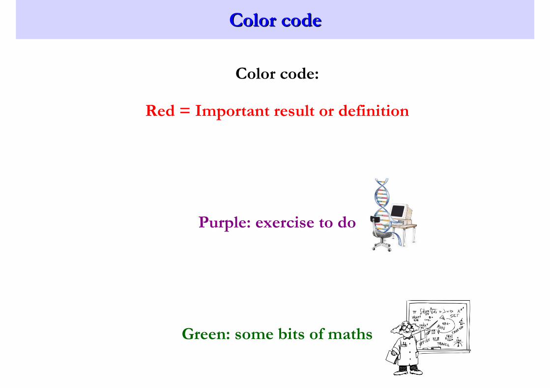
Population genetics: 4 evolutionary forcesPopulation genetics: 4 evolutionary forces

random genomic processes

(mutation, duplication, recombination, gene conversion)

naturalnatural

selectionselection

random demographic

process (drift)

random spatial

process (migration)

molecular diversitymolecular diversity

Lets look at genetic drift

WrightWright--Fisher model, genetic drift and neutral theoryFisher model, genetic drift and neutral theory

Neutral theoryNeutral theory

� Introduced by Motoo Kimura in 1960s, big controversy at the time.

� Can we explain all polymorphism data without the action of natural selection?

� Kimura: Most polymorphisms that occur do not influence the fitness of an

individual,

� thus these polymorphisms are not subjected to selection

� these mutations would evolve neutrally

�mutations at silent or degenerate sites do not change the Amino Acid BUT

may or may not evolve neutrally

� some non-synonymous mutations do not affect fitness (change in Amino

Acid does not affect the fitness) BUT may or may not evolve neutrally

Neutral theoryNeutral theory

� Neutral theory = most changes in allele frequencies in a population can be

attributed to genetic drift

� Why?

� When a mutation arise in a gamete of an individual, many things can happen:

� the carrier of the gamete must survive to reach the reproductive age,

� that gamete must be fertilized and develop an embryo,

� the embryo has to be viable to be at the next generation.

� Genetic drift means that mutation creates new alleles which by chance

� can rise in frequency and spread in a population,

� or they can get lost.

Neutral theoryNeutral theory

� We need a model to explain how genetic drift occurs

� and then use it to derive expectations on what polymorphism we should observe in

DNA sequences

� This model is based on how a population of individuals reproduce over time

� Important: to demonstrate that a given trait or polymorphism pattern is due

to selection, you MUST disprove alternative neutral explanations!

The WrightThe Wright--Fisher modelFisher model

The Wright The Wright –– Fisher modelFisher model

� Fundamental model in population genetics

� Assumptions (check list):

� Constant population size

� Discrete and non-overlapping generations

� Random mating (= panmixia)

� Equal sex-ratio

� 2N haploid individuals = N diploid individuals (with two allele each)

� One locus

�No recombination

The Wright The Wright –– Fisher modelFisher model

� How does it work?

� Let us assume 10 haploid individuals at generation t

� The offspring generation is obtained from the parents as follows:

� constant population => 10 individuals at generation t+1

� each individual from the offspring picks a parent at random from generation t

� connect parent and child by a line

� each offspring inherits the genetic information of the parents

The Wright The Wright –– Fisher modelFisher model

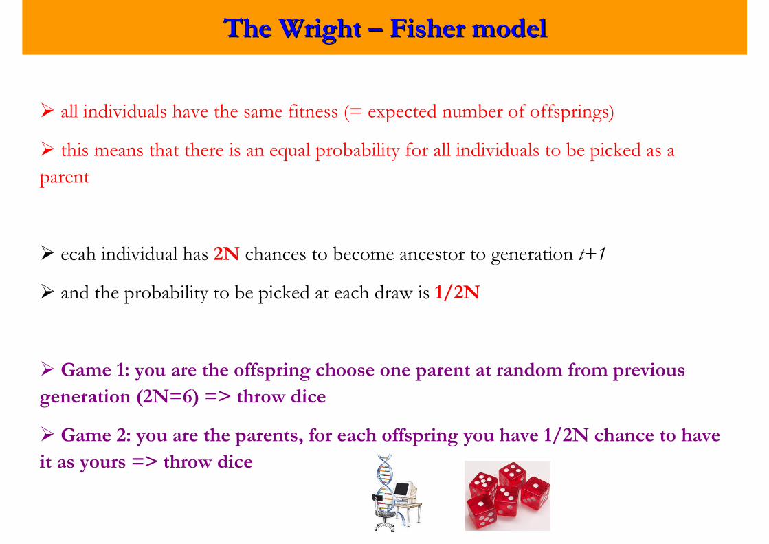
� all individuals have the same fitness (= expected number of offsprings)

� this means that there is an equal probability for all individuals to be picked as a

parent

� ecah individual has 2N chances to become ancestor to generation t+1

� and the probability to be picked at each draw is 1/2N

� Game 1: you are the offspring choose one parent at random from previous

generation (2N=6) => throw dice

� Game 2: you are the parents, for each offspring you have 1/2N chance to have

it as yours => throw dice

The Wright The Wright –– Fisher modelFisher model

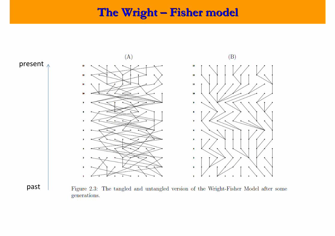
present

past

The Wright The Wright –– Fisher modelFisher model

present

past

The Wright The Wright –– Fisher modelFisher model

� all individuals have the same fitness (= expected number of offsprings)

� this means that there is an equal probability for all individuals to be picked as a

parent

� ecah individual has 2N chances to become ancestor to generation t+1

� and the probability to be picked at each draw is 1/2N

The Wright The Wright –– Fisher modelFisher model

Maths 1: Binomial distribution

Maths 2: Poisson distribution

Probability in the Wright Probability in the Wright –– Fisher modelFisher model

� for the Wright – Fisher model:

� n = 2N and p = 1/2N

� Can you calculate the expectation and variance for the binomial

distribution for this model?

� thus λ = np = 1

� Can you calculate the expectation and variance for the Poisson

distribution for this model?

�What is the difference between Exp and Var of the Binomial and Poisson?

� these are approximations

Probability in the Wright Probability in the Wright –– Fisher modelFisher model

� From the Poisson distribution, the probability of an individual not to leave

descendants is:

� P[X=0] = e-1 ≈ 0.37

� A fraction 1– 0.37 = 63% of all individuals have descendants at each generation

� in a randomly mating population, the present day population descent from a small

fraction of individuals a few generations ago

� this fraction is approximately ≈ 0.63t

� For a population fo size 2N = 10,000

� The population comes from: 10,000 ×××× 0.6315 ≈ 10 individuals from 15

generations ago

� The 9,990 other individuals did not leave descendants today

Genetic driftGenetic drift

Genetic driftGenetic drift

� It is a random stochastic process!!!!

�What it means for evolutionary biology: even if we know everything about a

population and ist biology, we cannot predict the state of the population in the

future

� Game 3: Two alleles (Red and White)

� you are the offsrpings in populations of sizes 2N = 6, 2N = 12 and 2N = 20

� p = 0.5 use the sheet with table to keep track of frequencies

� at each generation, the numbers on the dice for succesful reproduction changed

according to frequency of red allele at previous generation

� => throw dice

Genetic driftGenetic drift

Example 2N = 12

Throw dice for each offspring

Chance of being red = #red / 12

Here from 1 to 4 on the dice = reproduction

Genetic driftGenetic drift

� In fact we do not need to pick a random parent for each individual one by one:

� we can pick up this number from the binomial distribution, and use this as the

frequency at next generation

p = frequency of allele A 1-p = frequency of allele a

� frequencies at last generation in population with 2N individuals

� if more than two alleles we use the multinomial distribution

Genetic driftGenetic drift

� calculate from formula of the binomial distribution the probabilities:

� of loosing an allele P[X=0] with 2N= 10 for p = 0.5 ; p = 0.2 ; p = 0.01

� of loosing an allele P[X=0] with p = 0.5 and 2N= 10; 2N= 100; 2N=1000

� calculate from formula of the binomial distribution the probabilities:

� of fixing an allele P[X=2N] with 2N= 10 for p = 0.5 ; p = 0.2 ; p = 0.01

� of fixing an allele P[X=2N] with p = 0.5 and 2N= 10; 2N= 100; 2N=1000

� Can you correlate this with what you observe during the dice experiments???

Genetic driftGenetic drift

� Genetic drift = random change of allele frequency between generations

� Key facts about genetic drift:

� The probability of loosing/fixing alleles is HIGHER for small N (population

size)

� The probability of loosing/fixing alleles is HIGHER for small p (frequency)

Genetic driftGenetic drift

� Use Populus

� What about the time to fix or loose alleles?

� Look at the graphs, and try different values of

�N = 100, 500, 1000, 10 000

� initial frequency = 0.01, 0.1, 0.5, 0.99

� You can look at one or several loci: what does this mean?

Genetic driftGenetic drift

� Genetic drift = random change of allele frequency between generations

� Key facts about genetic drift:

� The probability of loosing/fixing alleles is HIGHER for small N (population

size)

� The probability of loosing/fixing alleles is HIGHER for small p (frequency)

� If loci are independent in the genome (physically not linked), each locus has

independent changes in allele frequency under genetic drift!!!!

The coalescent The coalescent -- 11

Kingman JF (1982)Kingman JF (1982)

Back to the Wright Back to the Wright –– Fisher modelFisher model

� Until now we have predicted the state of population at t+1 based on time t

This is the process forward in time

� Useful because it is logical and intuitive

� However, we can also follow the genealogy backward in time from present to

past

� Why????

� because most data we collect come from present day populations that we can sample

� The question becomes: what are the forces that have shaped the observed

patterns of diversity in our data (SNPs,…)??????????

� These forces have acted in the history of the population, so we look at the

geneaolgy

Back to the Wright Back to the Wright –– Fisher modelFisher model

present

past

Back to the Wright Back to the Wright –– Fisher modelFisher model

present

past

Back to the Wright Back to the Wright –– Fisher modelFisher model

present

past

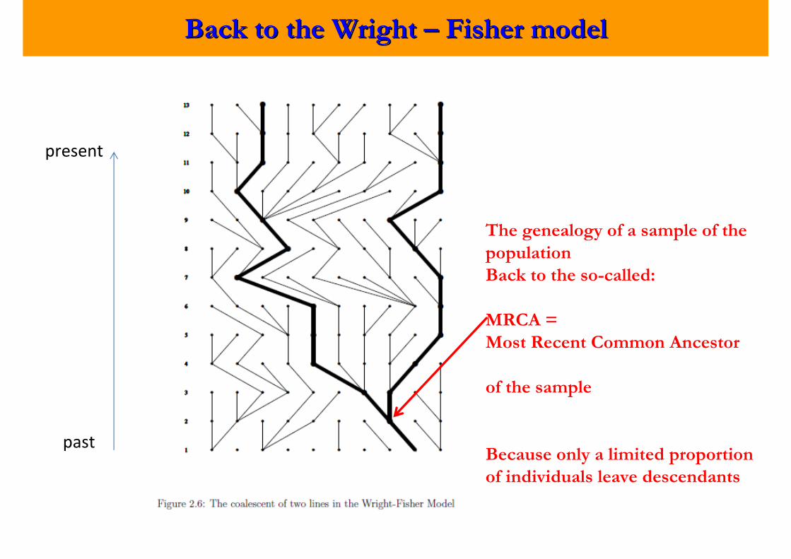
The genealogy of a sample of the

population

Back to the so-called:

MRCA =

Most Recent Common Ancestor

of the sample

Because only a limited proportion

of individuals leave descendants

The coalescentThe coalescent

� The idea is that we care only now about individuals which left descendants that are

found in our sample

� go to:

http://cgi-www.cs.au.dk/cgi-compbio/animate/html_animate?RecombParam

� Animation shows the Wright-Fisher model with only the important lineages

� Trees = rearrangements of the lines so that they do not cross

� Rho = 0

� Vary n = number of samples (individuals at present)

� How does the tree look like? Where are most of the coalescent events (recent or old?)

� When two lines fuse = coalescent event

The coalescentThe coalescent

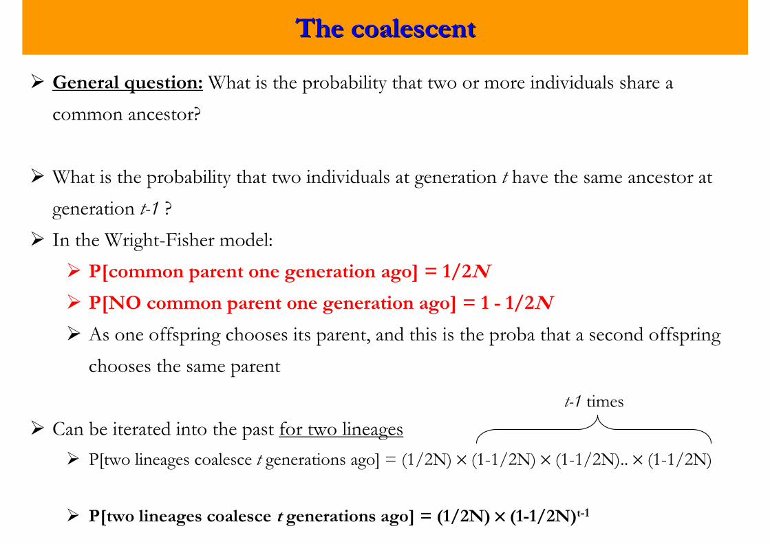
� General question:What is the probability that two or more individuals share a

common ancestor?

� What is the probability that two individuals at generation t have the same ancestor at

generation t-1 ?

� In the Wright-Fisher model:

� P[common parent one generation ago] = 1/2N

� P[NO common parent one generation ago] = 1 - 1/2N

� As one offspring chooses its parent, and this is the proba that a second offspring

chooses the same parent

The coalescentThe coalescent

� General question:What is the probability that two or more individuals share a

common ancestor?

� What is the probability that two individuals at generation t have the same ancestor at

generation t-1 ?

� In the Wright-Fisher model:

� P[common parent one generation ago] = 1/2N

� P[NO common parent one generation ago] = 1 - 1/2N

� As one offspring chooses its parent, and this is the proba that a second offspring

chooses the same parent

� Can be iterated into the past for two lineages

� P[two lineages coalesce t generations ago] = (1/2N) × (1-1/2N) × (1-1/2N).. × (1-1/2N)

� P[two lineages coalesce t generations ago] = (1/2N) ×××× (1-1/2N)t-1

t-1 times

The coalescent: two lineagesThe coalescent: two lineages

� P[two lineages coalesce t generations ago] = (1/2N) × (1-1/2N)t-1

� If you remember the geometric function ≈ exponential

� P[two lineages coalesce exactly t generations ago] = P[X = t] = p × (1-p)t-1

� P[X ≥ t] = (1 – p)t ≈ e-pt with p = 1/2N

Waiting time for coalescent two lineages

0

0,1

0,2

0,3

0,4

0,5

0,6

0,7

0,8

0,9

1

0 100 200 300 400 500 600 700 800 900 1000

time

P[X

> t

]

2N = 10

2N = 100

2N = 1000

Coalescence is faster in

small populations!!!

The coalescent: two lineagesThe coalescent: two lineages

� For a sample of size n, there are possible coalescent pairs

� The coalescent coalescent probability per generation is :

P[coalescence in sample of size n] =

So if Tn is the time until the first coalescent event:

2

2

n

N

2 2[ ] 1 exp

2 2

t

n

n nt

P T tN N

> = − ≈ −

What does this mean?

The coalescentThe coalescent

� We can calculate many aspects of a genealogical (coalescent) tree for a

population of size 2N

� Time to MRCA : E[TMRCA] = 4N (1 – 1/n)

� Time of coalescence of last two lineages : E[T2] = 2N

2N

2N/3

2N/6

2N/10

Most of the coalescence time

happens for low number of lineages

far in the past

Remember your exercise before

Times are functions of N

The coalescentThe coalescent

� We can calculate many aspects of a genealogical (coalescent) tree for a population of

size 2N

� The probability that a sample of size n conatins the MRCA of the whole

population = (n-1) / (n + 1)

� So typically a sample of 20 individuals is enough to study a population!

P[coalescent of smaple contains MRCA pop]

0

0,1

0,2

0,3

0,4

0,5

0,6

0,7

0,8

0,9

1

0 20 40 60 80 100 120 140 160 180 200

n = sample size

Pro

ba

The coalescentThe coalescent

� We can calculate many aspects of a genealogical (coalescent) tree for a population of

size 2N

� Beware we calculated only the Expectations

� However, the variance also exist, so that for the same n and 2N values, each tree is

be different in size and shape

� The size of the tree is given in units of 2N generations !!!!

The coalescentThe coalescent

� Important assumption of the coalescent model:

present

past

We assume that n << 2N

So that the probability of more than

2 lineages to coalesce is very small

P[3 lineages to coalesce] = (1/2N)2

This is small enough to be be

neglected if N is big, but not

always true

Next stepNext step

� How to use the coalescent to simulate sequence data?

� We need to introduce mutations on the tree