Evaluation of the Spectral Reflectance Pattern of Capsicum

SUNY College of Environmental Science and Forestry SUNY College of Environmental Science and Forestry

Digital Commons @ ESF Digital Commons @ ESF

Dissertations and Theses

Spring 5-1-2019

Evaluation of the Spectral Reflectance Pattern of Capsicum Evaluation of the Spectral Reflectance Pattern of Capsicum

annuum L. Treated with Fungicides and Grown Under Controlled annuum L. Treated with Fungicides and Grown Under Controlled

Conditions Conditions

Guillermo Ojeda [email protected]

Follow this and additional works at: https://digitalcommons.esf.edu/etds

Part of the Environmental Health and Protection Commons, and the Fungi Commons

Recommended Citation Recommended Citation Ojeda, Guillermo, "Evaluation of the Spectral Reflectance Pattern of Capsicum annuum L. Treated with Fungicides and Grown Under Controlled Conditions" (2019). Dissertations and Theses. 82. https://digitalcommons.esf.edu/etds/82

This Open Access Thesis is brought to you for free and open access by Digital Commons @ ESF. It has been accepted for inclusion in Dissertations and Theses by an authorized administrator of Digital Commons @ ESF. For more information, please contact [email protected], [email protected].

https://digitalcommons.esf.edu/

https://digitalcommons.esf.edu/etds

https://digitalcommons.esf.edu/etds?utm_source=digitalcommons.esf.edu%2Fetds%2F82&utm_medium=PDF&utm_campaign=PDFCoverPages

http://network.bepress.com/hgg/discipline/172?utm_source=digitalcommons.esf.edu%2Fetds%2F82&utm_medium=PDF&utm_campaign=PDFCoverPages

http://network.bepress.com/hgg/discipline/962?utm_source=digitalcommons.esf.edu%2Fetds%2F82&utm_medium=PDF&utm_campaign=PDFCoverPages

https://digitalcommons.esf.edu/etds/82?utm_source=digitalcommons.esf.edu%2Fetds%2F82&utm_medium=PDF&utm_campaign=PDFCoverPages

mailto:[email protected],%[email protected]

Evaluation of the Spectral Reflectance Pattern of Capsicum

annuum L. Treated with Fungicides and Grown Under

Controlled Conditions

By

Guillermo Francisco Ojeda

A thesis submitted in partial fulfillment

of the requirements for the Master of Science Degree

State University of New York

College of Environmental Science and Forestry

Syracuse, New York

May 2019

Department of Environmental Resources Engineering

Approved by:

Douglas J. Daley, Major Professor

Jaime Mirowsky, Chair, Examining Committee

Lindi J. Quackenbush, Department Chair

Gary M. Scott, Director, Division of Engineering

S. Scott Shannon, Dean, The Graduate School

ii

© 2019

Copyright

G. F. Ojeda

All rights reserved

iii

Table of Contents

List of Figures ........................................................................................................................................ iv

List of Tables .......................................................................................................................................... v

List of Appendices .................................................................................................................................. v

Abstract .................................................................................................................................................. vi

1 Introduction ..................................................................................................................................... 1

2 Literature Review ............................................................................................................................ 2

2.2 Remote sensing and proximal remote sensing ........................................................................... 4

2.3 Previous studies involving use of remote sensing ...................................................................... 7

3 Materials and Methods ................................................................................................................... 10

3.1 Location of the experiment ..................................................................................................... 10

3.2 Experimental Design .............................................................................................................. 10

3.3 Growing plants ....................................................................................................................... 11

3.4 Summary of data collected ..................................................................................................... 18

3.5 Data Processing...................................................................................................................... 20

3.6 Statistical Analysis Methods ................................................................................................... 21

4 Results ........................................................................................................................................... 22

4.1 Overview ............................................................................................................................... 22

4.2 Comparing treatments: mancozeb vs. control and copper vs. control ....................................... 24

4.3 Day by day observations ........................................................................................................ 28

5 Discussion ..................................................................................................................................... 29

5.1 Impact of this Work ............................................................................................................... 29

5.2 Assessment of Experimental Methods .................................................................................... 31

5.3 Future Work ........................................................................................................................... 34

6 Conclusion .................................................................................................................................... 35

Appendices............................................................................................................................................ 41

Vita ....................................................................................................................................................... 63

iv

List of Figures

Figure 1. Geographic distribution of Cu concentration in U.S. soils.......................................................... 4

Figure 2. Different spectral reflectance curves. ........................................................................................ 6

Figure 3. Materials used for sowing seeds. ............................................................................................. 11

Figure 4. Plants of pepper in their starting pots, covered with plastic film.. ............................................ 12

Figure 5. Plants of pepper in their starting pots, a week after sowing. ..................................................... 12

Figure 6. Transplant to seedling trays..................................................................................................... 13

Figure 7. Plants transplanted to individual pots. ..................................................................................... 14

Figure 8. Cage to spray plants, hand-spray and mixture of copper diammonia diacetate. ........................ 15

Figure 9. Field hyperspectrometer, laptop and leaf clip while performing a measurement. ...................... 16

Figure 10. Spectral sampling in a single band of the measurement device. ............................................. 17

Figure 11. Leaf damage due to the leaf clip and orange knot used to identify measured leaves. .............. 18

Figure 12. Reflectance curve for Plant 05 at day 3. ................................................................................ 20

Figure 13. Spectral curves corresponding to the plants (replications) sampled at day 7. .......................... 23

Figure 14. P-values for the F-tests and Tukey HSD tests at day 7. .......................................................... 23

Figure 15. Spectra of all replicates for days (a)1, (b)3, (c)7 and (d)14..................................................... 25

Figure 16. P-values of Tukey HSD tests and the F-testss. ....................................................................... 26

Figure 17. Ranges of wavelengths in which significant differences between treatments are observed in

more than one day. ................................................................................................................................ 27

v

List of Tables

Table 1. List of materials used ............................................................................................................... 11

Table 2. Band range, sampling interval and band width of the Fieldspec® 3 spectroradiometer .............. 17

Table 3. Days when data collection was performed, and datasets collected. ............................................ 18

Table 4. Summary of the spectral patterns collected ............................................................................... 19

List of Appendices

Appendix 1. Plots: Results of statistical analysis and spectra collected. .................................................. 41

Appendix 2. Script for R programming laguage ..................................................................................... 49

vi

Abstract

G.F. Ojeda. Evaluation of the Spectral Reflectance Pattern of Capsicum annuum L. Treated with Fungicides

and Grown Under Controlled Conditions. 34 pages, 4 tables, 17 figures. Bibliography style: IEEE.

The spectral response pattern of Capsicum annuum L. grown under controlled greenhouse conditions and

treated with the fungicides mancozeb (an organic pesticide) and copper diammonia diacetate (a copper-

based pesticide) was determined using proximal hyperspectroscopy. An ANOVA and Tukey HSD test

were performed for each wavelength from 350 nm to 2500 nm. The spectral reflectance of treated plants

showed significant difference (α=0.05) in the regions of the spectra from 414 nm to 523 nm, 583 nm to 697

nm and 1909 nm to 1953 nm for the detection of mancozeb up to seven days after the application of the

treatment and in the regions from 737 nm to 1898 nm and from 1986 nm to 2432 nm for the detection of

copper diammonia diacetate up to seven days after the application of treatment.

Keywords: hyperspectral response, pesticides, mancozeb, copper diammonia diacetate, remote sensing.

G. F. Ojeda

Candidate for the degree of Master of Science, May 2019

Douglas J. Daley, MS

Department of Environmental Resources Engineering

State University of New York College of Environmental Science and Forestry,

Syracuse, New York

Douglas J. Daley

1

1 Introduction

In the 20th century, the introduction of machinery and pesticides in the agricultural activities allowed

humanity to increase the world population at a rate never seen before in history, but this did not come

without threats to the environment and human health. Many pesticides introduced at this time, such as

mercurial based, were toxic and represented an important threat to the environment [1] [2] [3]. As decades

passed, other types of pesticides were developed, still dangerous for human beings and the environment,

but to a lesser extent. Broad-spectrum pesticides are less common in the market and are being replaced by

more specific ones (therefore, preventing farmers from harming living species that are not a threat to their

crops), have less toxicity in human beings (reducing hazards for workers and the surrounding population),

or may have a shorter time of decay (allowing an application closer to the harvest period and preventing

pesticide remnants to be present in the crop when it is ingested by human beings). Authorities of each

country regulate by laws what pesticides can be used. However, pesticides can still be present in the final

product, in a concentration that can be hazardous [2] [3].

Remote sensing has been used widely to monitor surface features. Satellite-based remote sensing in

agriculture has been used to assist in climate and soil assessment, land classification and crop inventories,

productivity estimations, obtaining stress indexes and identifying crop diseases [4]. The use of it in the

detection of pesticides applied to vegetation has been discussed before [5] [6] [7] and although satellite

remote sensing has been cited, other approaches such as drone-based and proximal remote sensing has been

given importance in recent years [8] .

Evaluating the spectral pattern of plants treated with pesticides can provide a valuable tool to detect

remnants of pesticides prior to harvesting for human consumption [6]. The research objective of this

experiment was to evaluate the spectral response of plants of Capsicum annum L. plants that were treated

with an organic fungicide, mancozeb, and a copper based fungicide, copper diammonia diacetate. Both

2

mancozeb and copper based pesticides are commonly used in the agricultural activity in many countries in

the world [9] [10] [11].

2 Literature Review

2.1 Agricultural Fungicides

2.1.1 Mancozeb

Mancozeb is a fungicide with protective action used in the production of field crops, fruit, nuts, vegetables,

ornamentals. The International Organization for Standardizations (ISO) defines mancozeb as “a complex

of zinc and maneb, containing 20% of manganese and 2.55% of zinc, the salt present being stated (for

instance, mancozeb chloride)” [12]. It belongs to the family of dithiocarbamates, which has a history that

can be tracked back to the 1930’s. Some compounds of this family became very popular from the 1940’s

onwards, being used to replace the popular Bordeleaux mixture in the production of some crops. In 1962,

Rohm and Haas registered the zinc ion complex of maneb, also known as mancozeb, which became a great

commercial success, being used in over 70 crops [13].

Today, Dow Agrosciences is the main registrant and producer of mancozeb and the product is sold by this

company in around 120 countries worldwide. Although the use of mancozeb is significant alone, it is present

in commercial formulations of other active principles such as benalaxyl, dimethomorph, myclobutanil or

even copper, among other fungicides [13].

Mancozeb is considered to present a low risk as a health and environmental hazard. In human beings, some

of the mentioned effects in humans are skin irritation, increase of weight of the thyroid, thyroid lesions and

tumors [14]. On very high doses in laboratory conditions it causes birth defects in mammals [12].

3

2.1.2 Copper-based pesticides

Copper pesticides probably became relevant due to the accidental discovery of the fungicidal properties of

Bordeleaux mixture, a mixture of copper sulphate and lime [11]. It was in 1882 when Pierre Marie Alexis

Millardet first reported of the use of Bordeleaux mixture as a fungicide [15], although there is evidence that

others used copper as a fungicide before than him [16].

While the benefits of copper sulphate have been known for decades, their negative environmental impact

has become relevant, and contamination with copper products in agricultural fields is currently a matter of

concern [9] [11] [17]. In Europe, copper-based fungicides have been used intensively over the decades

specially in vineyards and in other crops such as apples, avocado, tomatoes or potatoes. The long-term side

effect of the intensive use of copper is an accumulation of this metal in certain agricultural soils.

Investigations have shown that high concentrations of copper can affect adversely microbial and

earthworms’ communities present in these soils. Copper-based fungicides also present a risk for human

beings: inhalation of copper-based fungicides can lead to chronic respiratory problems such as lung-

carcinoma, liver diseases and neurological diseases [17] [9]. When ingested, copper may cause gastric

irritation, abdominal pain, nausea, vomiting, diarrhea [18]. There is not an internationally accepted level of

copper concentration in soils that is considered dangerous. However, one of the most cited guidelines was

proposed by the Finnish and Swedish legislations for soil contamination, which state that a concentration

of 100 mg kg-1 requires further assessment, and a value of 150 mg kg-1 denotes an ecological or health risk.

Other authors proposed 5-30 mg kg-1 as an appropriate value in soils since lower concentrations result in

plant deficiency, and higher may lead to toxic effects [9].

In the United States, a study by Holmgren et al. indicates that high concentrations (greater than 20 mg kg-

1) can be found in Florida, Michigan and New York, reflecting the agricultural management practices that

included the use of copper-based fertilizers and pesticides, and in California, probably reflecting

mineralization and the younger geological age of the area [19]. Figure 1 demonstrates a map generated by

Holmgrem et al. In it, the dotted lines are delimitations of areas for the study. The bold numbers represent

4

the means of the data within the selected areas (concentration of copper in mg kg-1), while the small numbers

are codes for county average concentrations.

Figure 1. Geographic distribution of Cu concentration in U.S. soils. Holmgren, 1993.

According to the United States Environmental Protection Agency (EPA), copper has generally moderate to

low toxicity (toxicity categories II, III and IV) based on acute oral, dermal and inhalation studies in animals,

but some studies indicate that some copper species may cause severe irritation (toxicity category I), such

as copper sulphate or cuprous oxide. However, EPA also mentions that in humans beings copper deficiency

is more common than toxicity from the excess [18].

2.2 Remote sensing and proximal remote sensing

As defined by Lillesand et al. remote sensing is the science and art of obtaining information about an object,

area or phenomenon through the analysis of data acquired by a device that is not in contact with the object,

area, or phenomenon under investigation. The device in question normally collects data, which is analyzed

5

to obtain the information needed [20] . Nansen defines Proximal remote sensing as the acquisition and

classification of reflectance or transmittance signals with an imaging sensor mounted within a short distance

(under 1 m and typically much less) from target objects [21]. The definition provided by Lillesand et al. is

more comprehensive than the one provided by Nansen, not only regarding to the distance from where the

device (or sensor) collects data, but the type of phenomena that the sensor detects: Nansen explains that the

sensor in question detects reflectance of transmittance [21], while under Lillesand’s definition, the sensor

could detect any other type of phenomena, including gravity [20]. Also, Nansen explains that an imaging

sensor must be used, indicating that the device should make a visual representation, or image, of the data

collected, while Lillesand only states that what we are collecting is information, a more comprehensive

term.

Reflected, Absorbed and Transmitted Energy of a Surface. When an incident beam of light impacts a

surface, part of the incident energy that comes with it will be absorbed by this surface, another part will be

transmitted, and the rest will be reflected. In other words:

Ei(λ) = Ea(λ) + Et(λ) + Er(λ)

where Ei is the incident energy, Ea is the absorbed energy, Et is the transmitted energy and Er is the

reflected energy, these energy components being a function of the wavelength, λ. The proportions of energy

absorbed, transmitted and reflected can vary significantly depending on the wavelength under study and

the properties of the surface we are studying.

The differences in the absorption, transmittance and reflectance allow us to distinguish different properties

of a surface by evaluating multiple wavelengths or ranges of wavelengths at a time [20].

The reflected component of the equation is of particular importance in the remote sensing system: most of

the remote sensors operate in wavelengths in which reflected energy predominates. If we calculate, for a

given wavelength, the percentage of the incident energy that is reflected, we obtain the spectral reflectance

𝜌(λ):

6

𝜌(λ) = Er(λ)

Ei(λ)

If we consider a broad enough range of the spectra and plot a graph of the spectral reflectance as a function

of the wavelength, we obtain a spectral reflectance curve, which will vary between different surfaces types

or objects. In other words, the spectral reflectance allows us to study or identify the properties of different

features (Figure 2) [20].

Figure 2. Different spectral reflectance curves. Lillesand & Kiefer, 2008.

7

Hyperspectral sensing. Hyperspectral sensors can collect data that enable the construction of a spectral

reflectance curve. As opposed to the traditional broadband system sensors, hyperspectral sensors can obtain

much more detailed information about the surface under study. Some applications of hyperspectral sensing

include determinations of surface mineralogy, water quality, soil type, vegetation type, leaf water content

and canopy chemistry [20]. For this reason, a hyper-spectroradiometer is well suited to the type of study

this thesis performed.

2.3 Previous studies involving use of remote sensing

Detection of pesticides using hyperspectral imaging. Sun and Zhou performed an experiment where

lettuce was grown under controlled conditions and sprayed with different organic phosphorus pesticides.

The main wavelength of each molecule pesticide was identified using hyperspectral imaging and Chemical

Molecular Structure Wavelet Transform. Residues of pesticides in leaves were successfully identified and

Sun and Zhou concluded that the spectral response of each pesticide produces a different spectral response,

even when belonging to the same family [22]. Sun and Zhou also identified residues of dimethoate in lettuce,

after spraying variable concentrations of the pesticide. Chlorophyll fluorescence spectra (wavelength of

300 to 510nm) and the spectra of wavelengths 870 to 1780 nm were evaluated. A different spectral pattern

for each initial concentration of the pesticide was identified [6]. Shao used visible and near-infrared

hyperspectral imaging and Raman spectroscopy to identify the pesticides glyphosate and butachlor in

Chlorella pyrenoidosa. By using Successive Projections Algorithms and a model of linear discriminant

analysis in the hyperspectral data a model was generated, which could identify the corresponding pesticides

with a correct identification rate that reached 100% for the cases tested. By using a partial least squares

discriminant analysis in the Raman spectrometry data, the correct identification rate of the model generated

reached 90%. Shao suggested that hyperspectral imaging and Raman spectroscopy can be complementary

as an effective way to indirectly characterizing pesticide varieties [23]. Jiang successfully detected

chlorpyrifos (an organophosphorus pesticide) residues in mulberry leaves (Morus sp.). The experiment took

place in the open, in a farm in Zhen Jiang province, China. It consisted in spraying different doses of the

8

pesticide, collecting the leaves 2 days afterwards, and acquiring a hyperspectral image of those leaves. He

used partial least squares regression (PLSR) to determine the most significant wavelengths to identify this

pesticide [24].

Spectral Reflectance Analysis to characterize vegetation growing under stress or in a contaminated

environment. Carter analyzed the spectral pattern of plants in different conditions including exposure to

herbicides, pathogens, dehydration and others stress factors and studied which wavelength ranges were

affected. For herbicides the affected ranges were 405-409 nm, 519-573 nm, 688-735 nm, 1384-1401 nm,

1875-1905 nm. Carter used an ANOVA, with alpha=0.05, and a Dunnet test for means comparison [7]. Shi

et al. compiled an extensive literature review about the most relevant studies that used visible and near-

infrared reflectance to estimate the presence of heavy metals in soils of diverse areas: Deltas, suburban

areas, river margins, agricultural areas, mining areas and lakes. The algorithms used in the statistical

analysis in these publications included Multilinear Regression, PLSR and Artificial Neural Networks, and

indicate a clear predominance of PLSR as a chosen algorithm when analyzing hyperspectral data. The

success of the studies reviewed were variable, and Shi et al. acknowledged that using hyperspectral imaging

to map heavy metals faces many challenges [25]. Arellano took more than 1100 leaf samples of vegetation

from healthy and oil-contaminated areas the Amazon forest. Hyperspectral data captured by the Hyperion

satellite was used to calculate vegetation indexes such as the normalized difference vegetation index and

ratio vegetation index and used them as indicators for contamination. This study led to the identification of

areas that present vegetation with a stress pattern associated with the presence of the contaminant. [26].

Spectroradiometers and optical technologies in food quality in general. Cen and Ye make reference to

several studies that have used near infrared spectroscopy in the study of food quality. However, because of

the lack of techniques and knowledge of spectral analysis, the developed procedures are limited to

laboratory conditions. Some of the studies addressed include the adulteration of beverages, evaluation of

milk and dairy products, differentiation of wine, determination of free fatty acids [27] . Huang studied the

advantages of hyperspectral imaging in food quality, describing it as a non-destructive and fast method that

9

was improved with the advancements of computer technology and instrumentation engineering. According

to Huang, red-green-blue color vision systems have been successfully applied when evaluating external

characteristics of certain types of foods but have limited reliability when evaluating internal characteristics.

The near-infrared (NIR) spectra, although more promising when quantifying chemical components than

other regions of the spectra, has proved inefficient when it comes to heterogeneous materials such as meat,

if there is not spatial information about the food being analyzed. Hyperspectral imaging, when used in the

field of food quality evaluation, has the advantage that can obtain both spectral information for wavelengths

from 300 - 2600 nm and spatial information, thus becoming more popular in this field. Products mentioned

to have been studied with hyperspectral imaging include fruits such as apple, citrus, peach, oranges, among

others [28].

Analysis of reflectance to identify differences in the spectra of features. Ferreira compared the

reflectance spectra of leaves of 21 tree species. The spectral pattern was obtained making use of a

Fieldspec®3 spectroradiometer, and an ANOVA test was performed for each wavelength ranging from 350

to 2500 nm and obtained the F-statistic followed by a Tukey HSD test. Ferreira identified which specific

wavelengths were statistically different between each species [29]. Khalegi successfully identified three

different minerals in a volcanic-sedimentary area in central Iran using Short wave infra-red imaging data

was obtained from the Aster satellite [30].

10

3 Materials and Methods

The experiment of this thesis consisted in raising plants of Capsicum annuum, under controlled conditions,

at the Old Greenhouse of ESF campus. Plants were separated in three groups, two of them treated with a

known dose of copper diammonia diacetate and mancozeb, and the third group used as a control (which

was sprayed with water only). Leaves from plants were measured four times over two weeks, and their

spectral response was measured by using a Fieldspec 3® spectroradiometer. The hyperspectral data was

collected, it was processed to determine whether there is a statistical difference in the spectral response

among the treatments, as well as how many days this difference could be detected.

3.1 Location of the experiment

The experiment took place at the germination chamber in Illick Hall and at the Old Greenhouse, both located

in the State University of New York, College of Environmental Sciences and Forestry campus address 1

Forestry Drive, Syracuse, New York, 13210.

3.2 Experimental Design

The experimental design was defined as follows:

Type of experiment: Completely Randomized Design

1. Factors:

a. Pesticides (3 treatments – 10 replications per treatment):

i. Control – No application of pesticides, only water spray

ii. Pesticide A – Mancozeb

iii. Pesticide B – copper diammonia diacetate (copper-based pesticide)

2. Dependent variable:

a. Reflectance spectra:

i. Spectral bands measured (2150 bands per measurement belonging to the

Red, Green, Blue and Near Infrared regions of the spectra)

Randomization was done after the plants were assigned a number. A script in R-Studio was used to perform

the random assignment of treatments.

11

3.3 Growing plants

Seed sowing. Sowing started on October 29, 2018. To achieve a proper germination, seeds were sowed in

seven groups of 16 per 0.5 L pot. Soil mixture was watered properly, then placed in the pots, which had

been sanitized properly. Seeds were gently placed on top of the soil surface evenly spaced one from each

other, then covered with approximately 2 millimeters of vermiculite. Pots were then covered with a plastic,

transparent foil, and left in the germination chamber of Illick Hall, with permanent artificial lights, for a

week.

Table 1 shows a list of materials used and their providers.

Table 1. List of materials used

Material Provider

Seeds of Capsicum annuum L. “Pepper Bell”

var. “California Wonder”

David’s Garden Seeds and Products (San Antonio,

Texas)

Soil Mixture “Miracle Go – Seed Starting

Potting Mix for Fast Root Development”

LOWE’S Garden Center

Vermiculite “Sta Green Horticultural

Vermiculite”

Staff of SUNY – ESF.

Seedling plates “Blissun 72 Cell Seedling

Starter Trays”

Windbow LLC.

Soil Mixture “Sta-Green Potting Mix” LOWE’S Garden Center

Liquid Copper Fungicide (Copper Diammonia

Diacetate)

Southern AG

Mancozeb flowable Bonide Inc.

Figure 3. Materials used for sowing seeds.

12

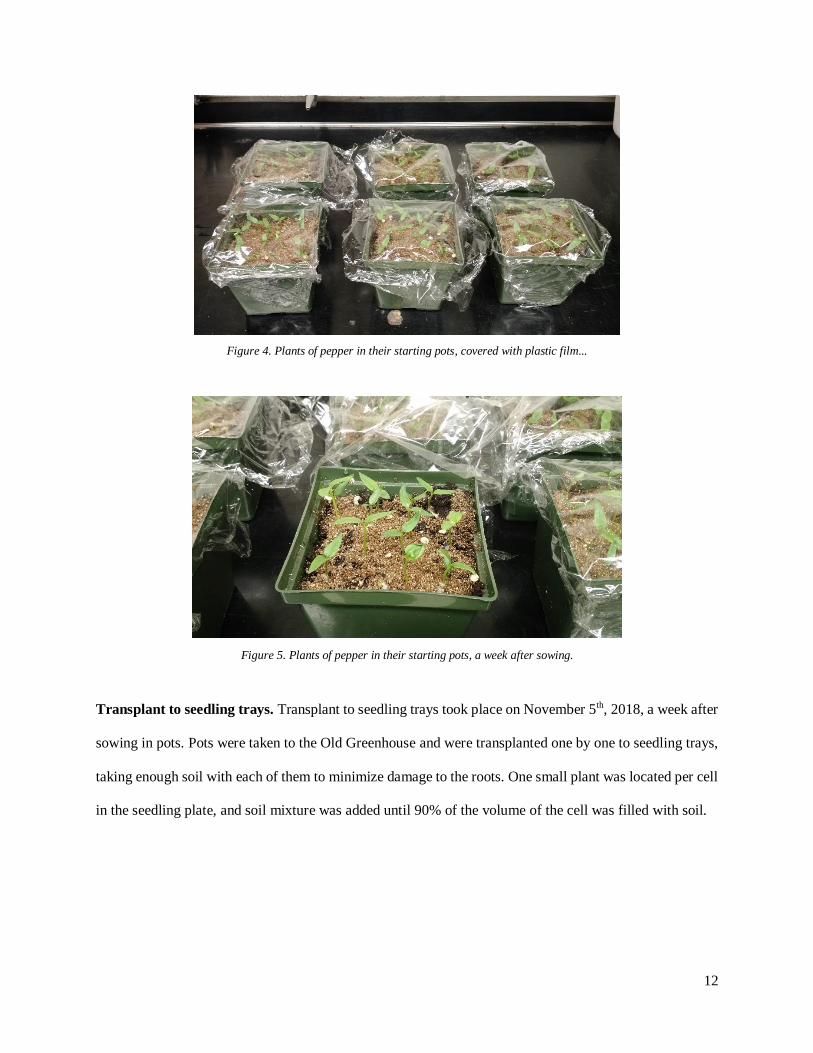
Figure 4. Plants of pepper in their starting pots, covered with plastic film...

Figure 5. Plants of pepper in their starting pots, a week after sowing.

Transplant to seedling trays. Transplant to seedling trays took place on November 5th, 2018, a week after

sowing in pots. Pots were taken to the Old Greenhouse and were transplanted one by one to seedling trays,

taking enough soil with each of them to minimize damage to the roots. One small plant was located per cell

in the seedling plate, and soil mixture was added until 90% of the volume of the cell was filled with soil.

13

Figure 6. Transplant to seedling trays.

Water was provided at least 3 times per week, ensuring field capacity with every addition of water. Once

seedlings displayed their second leaf, only manual irrigation was performed, and no water spray was used

for the remainder of the experiment. Artificial light was provided, aiming to ensure a 14-hour cycle, and

temperature was ensured to be at least 62°F (16°C). However, the timer that controlled the artificial lights

began to malfunction, at an unknown date. The device was replaced (at about day 25 after transplant), and

the lights began to work properly thereafter. The Discussion section explains what this malfunction could

have implied.

Transplant to individual pots. When plants had enough size (visual determination), they were transplanted

to individual 0.9 L pots, on November 29. Pots were filled to about 80% of capacity with “Sta-Green Potting

Mix” before plants were transplanted into them. Once transplant was done, pots were watered assuring that

field capacity was reached.

14

Figure 7. Plants transplanted to individual pots.

Individual pots were kept at the Old Greenhouse and the conditions of artificial light and temperature

remained the same. Pots were watered once every two days, with 200 ml of water in every irrigation, even

after the pesticide treatments were applied. During irrigation, caution was practiced in order that leaves are

not touched by water and would not wash-off the pesticides.

Application of fertilizer. By the start of January 2019, plants began to display symptoms that can be

attributed to lack of nitrogen, despite the fact that the potting mix used displayed the text “no fertilization

needed for the first nine months”. Due to this reason, a dose of fertilizer was applied with the irrigation

water. Dose applied was 200 ppm as recommended by other publications [31] [32] with an irrigation volume

of 200 ml per plant. This procedure was repeated four times in two weeks at even intervals and, after that,

once per week.

Application of Treatments. Treatments were applied taking into consideration the manufacturer

recommended doses. In the case of copper diammonia diacetate, the recommended concentration is 15 mL

to 30 mL (3-6 teaspoons) of commercial product per gallon of water. Concentration used was 22.5 mL per

gallon. Considering the concentration of the active principle in the commercial product (27%), this results

in a mixture of roughly 6 ml of active principle per gallon, or 1.6 ml/ L (1.6:1000). In the case of Mancozeb,

the used dose was 6ml of product per liter of mixture. Considering the concentration of the active principle

(37%), the final concentration in the mixture was 2 ml/L, or 2:1000. Control treatment had no dose of

pesticide, and the application consisted of only water.

15

The application of pesticides took place in January 7, 2019 and was done by making use of three different

hand sprayers (one for each treatment). The volume sprayed on each plant varied with the size of the plants

and their leaves but was around 15 ml per plant. To prevent the drift of the pesticide when spraying the

plants, they were sprayed in a small plastic cage that was covered in plastic, with one of its sides open so it

the person in charge could spray the plant conveniently.

Figure 8. Cage to spray plants, hand-spray and mixture of copper diammonia diacetate.

Data collection. The first hyperspectral measurement was made one day after the application of pesticides

(Day 1). Additional measurements were taken on days 3, 7 and 14.

For the purpose of this thesis and the corresponding experiment, it was assumed that the data collection

involved performing a type of proximal remote sensing that does not include the generation of imagery in

the traditional sense, but acquisition of reflectance data from the surface of plant’s leaves. Data was

collected by using a FieldSpec® 3 spectroradiometer, by Analytical Spectral Devices (ASD) Inc. The

wavelengths under study will be those that range from 350 nm to 2500 nm.

16

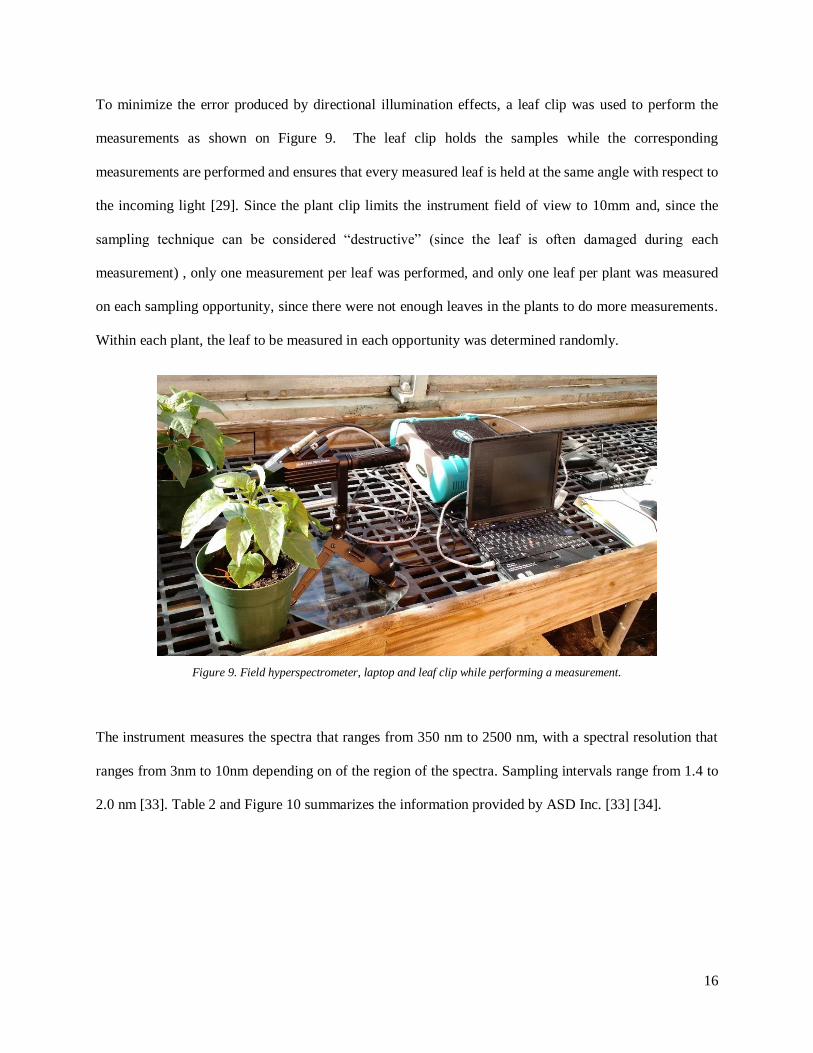
To minimize the error produced by directional illumination effects, a leaf clip was used to perform the

measurements as shown on Figure 9. The leaf clip holds the samples while the corresponding

measurements are performed and ensures that every measured leaf is held at the same angle with respect to

the incoming light [29]. Since the plant clip limits the instrument field of view to 10mm and, since the

sampling technique can be considered “destructive” (since the leaf is often damaged during each

measurement) , only one measurement per leaf was performed, and only one leaf per plant was measured

on each sampling opportunity, since there were not enough leaves in the plants to do more measurements.

Within each plant, the leaf to be measured in each opportunity was determined randomly.

Figure 9. Field hyperspectrometer, laptop and leaf clip while performing a measurement.

The instrument measures the spectra that ranges from 350 nm to 2500 nm, with a spectral resolution that

ranges from 3nm to 10nm depending on of the region of the spectra. Sampling intervals range from 1.4 to

2.0 nm [33]. Table 2 and Figure 10 summarizes the information provided by ASD Inc. [33] [34].

17

Table 2. Band range, sampling interval and band width of the Fieldspec® 3 spectroradiometer

Band Range (nm) Sampling Interval (nm) FWHM band width (nm)

350-1000 nm 1.4 nm 3 nm

1000-2500 nm 2 nm 10 nm

Figure 10. Spectral sampling in a single band of the measurement device. ASD Technical Guide, by Analytical Spectral Devices, Inc, 2010.

Plants were identified individually by numbering them. Previous researchers suggested that when

performing a spectral measurement with the leaf clip, leaves can be damaged, making it improper for future

measurements [35]. Therefore, when a leaf was measured, it was tagged to prevent from measurement of

that leaf again by mistake.

18

Figure 11. Leaf damage due to the leaf clip and orange knot used to identify measured leaves.

Four datasets were collected, as explained in Table 3.

Table 3. Days when data collection was performed, and datasets collected.

Day Date Dataset Collected

1 01-08-2019 Measurements one day after application of pesticide.

3 01-10-2019 Measurements three days after application of pesticide.

7 01-14-2019 Measurements seven days after application of pesticide.

14 01-21-2019 Measurements 14 days after application of pesticide.

RS-3 is the name of the software that displays the data collected by the Fieldspec® 3 spectroradiometer and

it allows to configure the number of spectral observations that are going to be taken and averaged to give a

result. In this case, 10 observations were made and averaged per every leaf sampled in a single sampling

opportunity. As shown in Table 3, the last day of data collection was 14 days after the application of

pesticides.

3.4 Summary of data collected

The data used in this study are the spectral measurements that were identified as explained in the Table 4.

19

Table 4. Summary of the spectral patterns collected

In Table 4, the columns “Spectra” correspond to the name of the data collection associated to the spectral

reflectance measured. This way, for example, the spectra “Plant05d3” corresponds to the measurement

taken from the plant identified as “05”, the day 3 of the experiment (since the pesticides were applied in the

“day 0”, “day “3” is the third day after the application of pesticides). In total, 120 “spectra” were collected.

As already mentioned, each “spectra” in the table is not a simple datum but consist of 2150 [wavelength,

reflectance] data pairs that, together, define the reflectance spectral pattern for the region of wavelengths

20

from 350 nm to 2500 nm. By plotting each data pair in a scatterplot, with the wavelength on the X axis, and

the reflectance on the Y axis, we obtain the graphic representation of the spectral curve [20]. For example,

the curve for the spectra “Plant05d3” has the following shape (Figure 12):

Figure 12. Reflectance curve for Plant 05 at day 3.

We can observe that this curve has a similar appearance to the spectral response curves of many other

vegetation types [36].

3.5 Data Processing

RStudio was used to process the 120 spectral patterns that were collected (10 plants per treatment, 3

treatments, 4 days of measurements), with each spectral pattern composed of 2150 wavelength: reflectance

pairs.

RStudio is an integrated development environment (IDE) for the computer programming language R [37].

They are powerful tools that support a wide range of computations and statistical procedures. They provide

certain advantages: they are open-source resources and can be obtained for free from the internet which

makes it very convenient for independent researchers or those with limited economic resources for their

researches, it is the choice of many statisticians and academics who, at the same time make contributions

21

to improve packages designed for it and it runs well in many computer platforms including Microsoft

Windows, Mac OS X, and Linux. They have the disadvantages that they are more difficult to use than other

statistics packages like SPSS, and they are slower to process data compared to other languages like C or

FORTRAN [38].

3.6 Statistical Analysis Methods

To analyze the data and find out whether a significant difference can be found in the spectra, an analysis of

variance (ANOVA) test and Tukey honest significant difference (HSD) test was performed separately for

each wavelength (from 350 nm to 2500 nm) and for each day.

ANOVA is a collection of statistical procedures for studying the relation between a dependent variable and

one or more independent variables. Analysis of variance models are a basic type of statistical model that

are concerned with the relation of one (or more) independent variable, and a dependent variable, but they

differ from regression models in respect that the independent variable may be qualitative [39], for this

reason it adapts to the type of study this thesis is performing. The F-test for equality of factor levels means

is a procedure that can tell us if at least one group of data is significantly different from at least another

group of data, and is commonly done in ANOVA tests, when comparing multiple groups of data (i.e.:

multiple treatments). The result of each F-test is associated to a “power of the F-test”, also called p-value,

that is the probability of making a mistake when assuming that at least one group is different from at least

another group of the ones considered, given the data under examination. However, the F-test will not tell

us which one of the groups of data is different from which other. To solve this problem, there are different

statistical procedures that will do so, and they are often used after one F-test has attained a p-value below a

certain threshold alpha. One of these tests is Tukey HSD test.

For this study, a Tukey HSD test was performed after every F-test. The result of each Tukey HSD test is

also associated to a given number of “power” values, one for each possible comparison between the

available treatments’ means. In our case, the possible comparisons in a Tukey HSD test (for each day and

22

each wavelength) are Copper vs. Control, Mancozeb vs. Control and Copper vs. Mancozeb. We will

only display the results of Copper vs. Control and Mancozeb vs. Control, since the most direct application

of these type of analysis would be to compare the presence of a given pesticide with the absence of it, not

to compare the presence of different types of pesticides among each other.

The chosen approach for the statistical analysis was the following: for every day of sampling (days 1, 3, 7

and 14) and for each of the 2150 wavelengths analyzed an ANOVA test was performed which included an

F-test, followed by a Tukey HSD test. This last test allows to identify in which bands of the spectra there

is a significative difference at each day, and among which treatments. By doing this we can determine

which wavelengths, in which days, present a significant difference between the treatments Copper vs.

Control and Mancozeb vs. Control. A confidence level (α) of 0.05 was used.

4 Results

4.1 Overview

Results are represented in different plots. For each day, one plot represents all the spectra collected and the

p-values of the F-statistic, and another represents the p-values for the F-statistic and of the pairwise

comparisons of treatments copper vs. control and mancozeb vs. control.

To assist the reader in understanding the spectral response curves, examine Figure 13 and Figure 14 which

show the results for one measurement on Day 7. Figure 13 illustrates the spectral pattern for each of the 30

plants (3 treatments, 10 replicates) measured in this day, along with the p-value for the F-statistic resulting

from the ANOVA performed for each wavelength. The horizontal dotted line represents the confidence

level α=0.05. When the p-value is less than 0.05, there is a significant difference between the control and

the treatment at that specific wavelength (alpha <0.05).

23

Figure 13. Spectral curves corresponding to the plants (replications) sampled at day 7. Different colors correspond to a

different treatment. The black curve corresponds to the p-values for an ANOVA test. The dotted red line indicates the value for α=0.05.

Figure 14. P-values for the F-tests (black) and Tukey HSD tests: Mancozeb vs. Control (red line) and Copper vs. Control (Blue

line). Values represented for each of the wavelengths measured at day 7.

Figure 14 shows the results of the p-values for a pairwise comparison of copper vs. control (in color blue)

and mancozeb vs. control (in color red). When one of these 2 curves go below the horizontal red dotted

line that represents α=0.05, there is a significant difference in the corresponding pair-wise comparison, at

those wavelengths. The p-value resulting of the ANOVA test is the curve of black dots.

24

4.2 Comparing treatments: mancozeb vs. control and copper vs. control

Figure 15 shows the spectra and p-values for the F-tests of each wavelength for each of the four

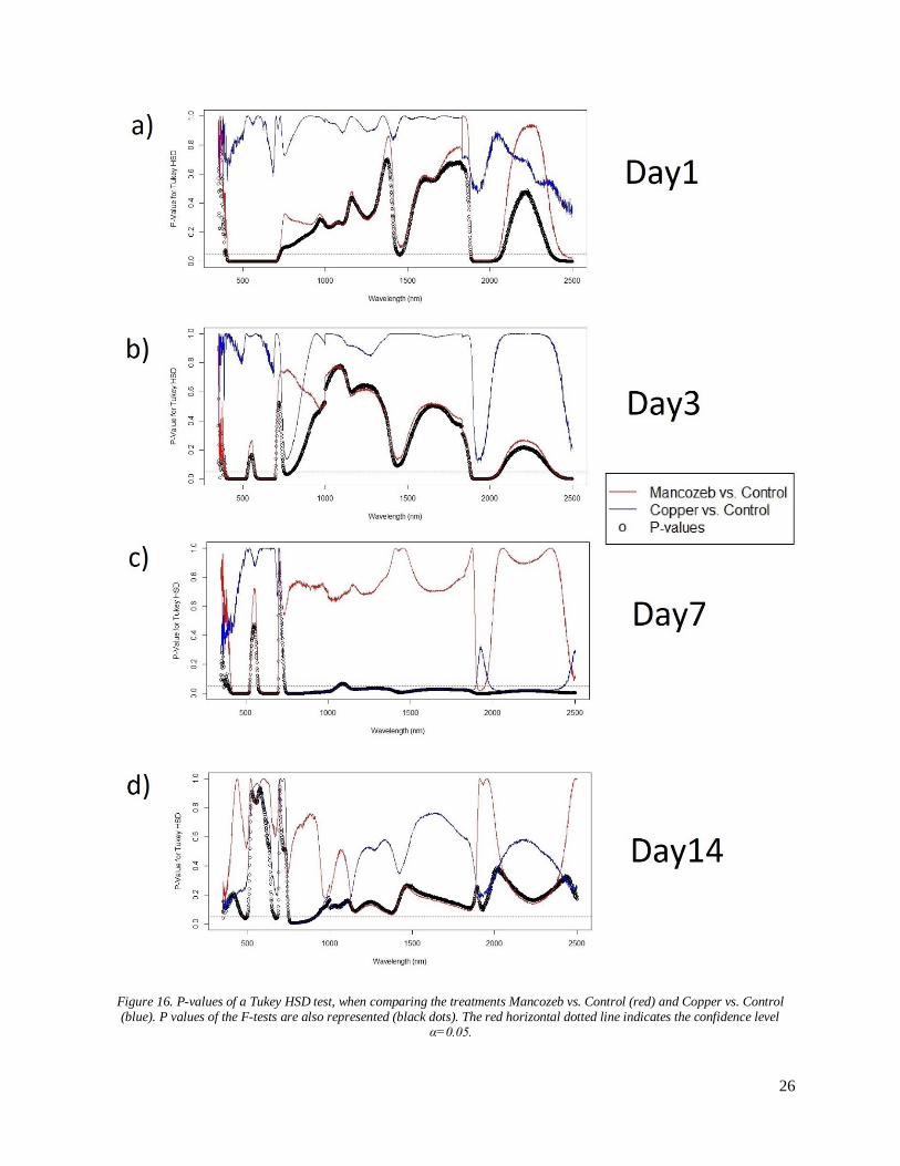
measurements. Figure 16 shows the p-value for pair-wise comparisons of Copper vs. Control and

Mancozeb vs. Control for a Tukey HSD test. The regions on the spectra with consistently low p-values

(less than 0.05 in more than one day) for the Tukey HSD test for these comparisons are highlighted with

rectangles in Figure 17 in color blue (for the comparison of copper vs. control) or red (for the comparison

of mancozeb vs. control). For this study, a region of the spectra is considered to have “consistently” low p-

values when they presented a p-value in more than one day under study; this means that for those regions

of the spectra the pair-wise comparison presents a significant difference.

25

Figure 15. Spectra of all replicates for days (a)1, (b)3, (c)7 and (d)14. Different colors correspond to different treatments. The black dotted line indicates the P-values for every F test. The horizontal red dotted line indicates the confidence level α=0.05.

26

Figure 16. P-values of a Tukey HSD test, when comparing the treatments Mancozeb vs. Control (red) and Copper vs. Control (blue). P values of the F-tests are also represented (black dots). The red horizontal dotted line indicates the confidence level

α=0.05.

27

Figure 17. Ranges of wavelengths in which significant differences between treatments are observed. P-values of Tukey HSD tests

(red and blue) and P-values the F-tests (black). Red and blue rectangles indicate bands ranges that showed significant differences for Mancozeb vs. Control and Copper vs Control respectively for more than one day.

28

The results presented in Figure 15 do not indicate which treatments differ from one another, only that at

least one is different. Therefore, we recur to the results of the Tukey HSD analyses, which are displayed in

Figure 16. These analyses indicate the following for treatments copper vs control:

• At days 1 and 3, the treatments copper and control are not significantly different for an α=0.05,

for any wavelength.

• At days 7 and 14, for and α=0.05 there is a significant difference in the wavelengths that range from

750-920 nm.

• Only at day 7, for an α=0.05, the bands that displayed a significant difference were 737-1898 nm

and 198-2432 nm, which corresponds to almost the entirety of the near infrared spectra (NIR) and

a considerable part of the mid infra-red.

For treatments mancozeb vs. control:

• For α=0.05, for days 1, 3 and 7 there is a significant difference in the reflectance of the following

wavelength ranges: 414-523 nm, 583-697 nm and 1909-1953 nm.

• For α=0.05 and considering both days 1 and 3 only, the wavelength ranges with a significant

difference in their reflectance were: 409-525 nm, 576-697 nm, 1893-2039 nm and 2441-2500 nm.

4.3 Day by day observations

For an α=0.05 In day 1 no significant difference in the reflectance of any wavelength was found

between the treatments of copper vs. control. For the treatments mancozeb vs. control, a significant

difference was found for the ranges of wavelengths: 409 nm to 720 nm, 1893 nm to 2043 nm, 2441 nm to

2500 nm.

In day 3, no significant difference in any wavelength was found for copper vs. control for an

α=0.05. For the treatment mancozeb vs. control, for an α=0.05, the wavelength ranges that presented a

29

significant difference were 386 nm to 524 nm, 576 nm to 697 nm, 1895 nm to 2052 nm and 2391 nm to

2500 nm.

In day 7, significant differences for the treatments copper vs. control with an α=0.05, were found

in the entire range of 737 nm to 1898 nm and 1986 nm to 2432 nm. For the treatments mancozeb vs.

control, the wavelengths with significant differences in their reflectance were 414 nm to 523 nm, 582 nm

to 697 nm and 1909 nm to 1953 nm.

In day 14, with an α=0.05 significant differences were found for copper vs. control for the

wavelengths 750 nm to 920 nm. No significant difference was found for mancozeb vs. control for a

significance α=0.05.

5 Discussion

5.1 Impact of this Work

In this experiment it was possible to detect the application of mancozeb up to seven days after its

application. The half-life of mancozeb in plants varies in literature from 4.29 days [40] to 10.6 days [41].

These values are consistent with the results obtained in this study, and this could imply that the spectral

reflectance of treated plants can be analyzed to assess the presence of mancozeb residues in plants within

the half-life period. Inorganic pesticides do not break down in the same way as organic pesticides, and the

“half-life” concept only applies to organic pesticides (those that contain carbon components) [42], so a

comparison of this kind cannot be addressed for the study of copper diammonia diacetate.

The spectral reflectance of copper is high for the NIR region, above 0.95 [43]. This could explain

the results of the spectral pattern observed at days 7 and 14, when a significant difference was found in the

NIR region of the spectra, specially at day 7, but not the results for days 1 and 3. This indicates that the

application of copper could be detected by studying the spectral reflectance of treated plants, but only after

7 days have passed since the application.

30

Unfortunately, similar experiments that use the same pesticides were not found in the literature to

be able to compare these results. However, these studies have achieved similar results in the sense that they

were able to identify regions in the spectra where the reflectance is significantly different for treated plants,

when compared to untreated plants. Jiang found that the optimal wavelengths to detect chlopyrifos were

400, 442, 701, 715, 722, 732 and 970 nm two days after its application [24]. Our results indicate that the

ranges 414-523 nm can be used to detect the application of mancozeb after seven days of the application,

which matches one region mentioned by Jiang. If we consider day 1 only, our results indicate that the entire

region from 400 nm to 750 nm can be used to assess the application of mancozeb, matching other regions

of the spectra that Jiang mentions as optimal wavelengths for the detection of mancozeb.

Sun et al. managed to identify 4 regions of the spectra that are of interest when attempting to find

significant difference when different pesticides (dimethoathe, acephate, phoxim, dichlorvos and

avermectin) are sprayed on lettuce, 2 hours after the application of pesticides: 875—1050 nm, 1050—1250

nm, 1350—1550 nm, 1650—1780 nm [22]. In this case, there is no coincidence with our results for days 1

and 3 for either mancozeb or copper. This could indicate that either not all pesticides produce the same

spectral response (as explained by Sun et al.) or that the spectral response of different plant species is not

affected in the same way when treated with pesticides. Other publication by Sun et al. also support this, in

which he found that the most promising wavelengths to detect an application of dimethoate are 902.13 nm,

931.79 nm, 1207.45 nm, 1433.02 nm and 1673.29 nm [6], none of those matching our results. Sun et al.

already mentioned that different pesticides can induce a very different change in the spectra of a plant, even

if they belong to the same family of pesticides. It should also be considered that different plants species can

react in different ways to the same pesticide, so it is possible that the change in the spectra when exposed

to a same pesticide is not the same for different plant species.

Ideally, performing studies like this one and after enough research and experimentation, a spectral

response could be identified for each combination of pesticide and plant species of interest, in a way that

could allow the detection of pesticides in crops or in a faster and more affordable way than traditional

31

methods, for large surfaces or volumes of food. An example of a use of this technology could be mounting

sensors in drones, which detect only the specific regions in the spectra where we expect to find the response

of a pesticide (to make them more affordable). In a similar way, evaluation of the spectral response pattern

to detect the nutritional status of plants, affliction by plagues, diseases or contamination of soil and water

could be investigated as other authors have proposed [7] [26] [25]. However, for these applications

challenges appear, for example spectral responses can vary for different weather or soil conditions, species

or phenological state of the plants.

5.2 Assessment of Experimental Methods

This study attempted only to determine whether a statistical difference between treatment can be

found, but an attempt for modelling the changes in reflectance values for different wavelengths was not

made. If we desire to find a model of the behavior of the spectral pattern as time passes after the application

of one pesticide, probably a good approach would be to group the bands that have proved significant in a

same treatment (that is, they present a low p-value after a Tukey HSD test), process the information with a

regression model. Other option would be to use an algorithm that considers the participation of each

wavelength, and determines which ones are the most important, such as PCR [44] or PLSR [45] which

other authors have used.

We have worked under the assumption that every leaf in the same plant behaves the same way,

which may not be true. For example, it is known that nitrogen tends to concentrate in the younger leaves if

there is a deficiency of it, or that the content of chlorophyll in each leaf can vary depending on how exposed

to sunlight it. Also, different individuals (plants) can behave differently simply because of having different

genetic composition (this experiment raised plants from seeds, not tissues from one same parent individual).

For these reasons, should the data from a similar experiment be used to fit a model, then a model with

nested random effects should probably be used [38] (leaf random effect, nested inside plant random effect).

32

This experiment did not attempt to explain in depth the reason why some ranges of bands are

different in one treatment with respect to another and the control. There are many chemical, physical and

physiological possible explanations for this, but the objective of this work was not to determine why does

a band change, but whether if it is possible to detect at least the effect of some sort of pesticide in some sort

of vegetal. Even so, to address the effect of a copper based pesticide in the reflectance, a good approach

could be to take into consideration the reflectance pattern of copper, which is above 0.95 in the NIR region

of the spectra [43]. This can explain why a significant difference in the reflectance spectra of the copper

treatment was found at day 7 in comparison with the control treatment, especially in the NIR region. Other

possible reason is that a physiological reaction takes place after the application of copper diammonia

diacetate, but its effect on the spectral reflectance will not be detected until more than 3 days have passed,

and most of them would disappear after 2 weeks.

It should be considered that there were at least three factors that may have been a source of

variability on the data collected. Two of them involved not having ideal growth conditions during plant

development at the greenhouse. First, it was noticed at about day 11 after transplant of peppers to individual

pots that the timer device that controlled the artificial lights at the greenhouse was not working properly,

making the amount of artificial light hours per day be unknown, but most likely less than half of the amount

needed. After 4 attempts of reconfiguration of the device it was noticed that the device would only work

properly (perhaps) for about 2 or 3 days, until it started working erratically again, for reasons unknown. As

a result, the timer device was replaced (at about day 25 after transplant), and the lights began to work

properly.

Second, the availability of nitrogen in the soil mixture was not enough. Originally, it had been

decided in the experimental design that the plants were not going to be fertilized, and instead a good quality

soil, with enough nitrogen, would be used. The main concern was that if fertilizers were applied, the size

of the leaves would grow significantly between measurements, making the amount of pesticide per cm2 of

leaf area decrease with elapsed time; this could have led to changes in the spectral pattern simply due

33

enlarged leaf size over time. To counterbalance the lack of fertilization, a commercial soil mixture was used.

Even when the commercial soil mixture stated that “no fertilization will be needed for nine months”,

symptoms of deficit of nitrogen appeared about 45 days after transplant to individual pots, and chemical

fertilizers had to be used to make sure plants stayed healthy. Nine days after the application of fertilizer,

visual inspection indicated that plants recovered, and the data collection began about 3 days after. This lack

of nitrogen before the application of pesticides may have affected the spectral measurements in some way

and could have induced additional variance in the measurements.

Third, there was an unexpected effect in the data collection that took place in nearly all

measurements during days 1 and 3. As explained in the Fieldspec3 manual [33], when the equipment is

activated it is constantly working, collecting and representing data (if it is connected to the computer with

the RS3 software running). The measurements taken were updated at a rate of about 1.5 seconds (that is, an

updated spectral pattern was displayed in the screen of the computer every approximately 1.5 seconds).

However, when clipping the leaf to take a measurement during days 1 and 3, a spectral curve for the same

leaf would shift slightly in almost every sample as time passed, making the curve update into another one

with all band’s reflectance values slightly less than the previous one. It would stabilize at about 30 seconds

to a minute after the leaf clip was clipped to the leaf, but it was assumed that this “stable” measurement

was incorrect: probably the clip damages the tissues in a way that affects the spectral measurement, until

the effect of this “damage” is stabilized. This effect did not appear in the measurements of days 7 and 14,

except when (only for curiosity purposes) a measurement was made in a few younger leaves, probably no

more than 1 week old. The “shifting effect” was present in these leaves. This could mean that, for reasons

to be discussed, this effect takes place when sampling young leaves only. Therefore, although an effort was

made to record the spectra as soon as the leaf-clip was clipped into the plants, some variability may have

been induced by the “shifting effect” during days 1 and 3, increasing the variance of the measurement. This

could be a reason why the copper treatment displayed no significant difference with respect the control

treatment.

34

5.3 Future Work

The practical application of this experiment is to demonstrate whether these two pesticides, copper

diammonia diacetate and mancozeb, can be detected after being sprayed on plants, in this case of red pepper.

As explained by other authors who have performed research on related subjects [22] [23] [28] , there are

many obstacles to implement this a as a technique of routine control in the food industry for different vegetal

species and pesticides, either by using proximal remote sensing or drone-based remote sensing. To name

some: the difference of growing plants in controlled conditions and the environmental conditions, the

interactions between the different species of plants, the effect of environmental conditions and of pesticides

used, doses of pesticides used, economic costs of implementation, etc. If this type of techniques used in

the food industry as a regular process, extensive research will be needed before, both under controlled

conditions and in the open environment.

We must take into account that in other environments (i.e.: where growth conditions are not

controlled), there are many other variables that can influence the spectral response of the plant, and therefore

can affect the spectral measurements collected, up to a point where it is not possible to find a significant

difference for any band. Conditions like rains could wash-off the pesticide from plant’s leaves, making it

less likely to be detected. Hunsche simulated a 5mm rain after applying mancozeb to apples seedlings and

concluded that 75% to 90% of the deposit of mancozeb would be washed off if the rain took place during

the first 24 hours after the application [46]. Most likely a wash off like this would limit the response of the

reflectance curve to a point where it would be much harder to identify if a plant had been effectively treated

or not. However, depending how long has it been since the rain took place, it is possible that the plant

develops a physiological response that can be identified in its reflectance curve, regardless the presence of

the pesticide. For the case of copper pesticides, rain could have a more reduced effect. Vincent et al. indicate

that copper products have better rain fastness than mancozeb and other pesticides, and in their studies

cuprous oxide and copper oxychloride managed to provide satisfactory disease control on citrus fruits after

35

71 mm of rainfall. They mention that respraying only seems necessary after heavy rains of wind-driven

rains [47]. For this reason, it could be possible to detect a change in the spectral response of plants after the

application of copper-based fungicides, even if a rain took place after its spraying.

Other factors that could affect the vegetal tissues altering their spectral pattern are low or high

temperatures, droughts or dry winds. These factors must be considered, if a similar procedure is used in the

open environment. Before this procedure can be applied in the food industry, more research is necessary.

Another aspect to consider in future experiments is that different companies use different

composition in their commercial formulations for the same pesticide. That is, only a fraction of the

commercial product is the active principle of the pesticide, or the molecule of interest. The rest corresponds

to other components that help the pesticide perform better (e.g.: better solubility of the product in water). It

is possible to measure the spectral reflectance of the product before applying to the plants as well and

compare the change of the spectra in sprayed plants with the reflectance of the commercial product itself.

To improve this experiment, more repetitions per treatments (more plants per treatments) could be

used, to reduce the variance within each treatment, and therefore allowing us to identify more bands were

potential changes could appear. Also, collection of data of treated plants that grew in the open environment

could be attempted, to verify if results are similar when growing in a greenhouse. Another good

improvement would be to make measurements during every day in two weeks, not only in four days, to

better describe the evolution of the spectral response.

6 Conclusion

The results of this experiment indicate that it is possible to use proximal sensing devices to tell

apart when plants of Capsicum annuum L. have been treated with copper diammonia diacetate, mancozeb,

or have not been treated at all, for the growth conditions in which this experiment took place. The most

promising bands that were observed in this case are 414 nm to 523 nm, 583 nm to 697 nm and 1909 nm to

1953 nm for the detection of mancozeb up to 7 days after the application of the treatment.

36

At days 1 and 3 no significant difference was found when comparing the treatments copper and control,

but the wavelengths from 750 nm to 920 nm displayed significant differences for both treatments at days 7

and 14. Specifically at day 7 significant differences in the reflectance was found in a broad spectrum of

wavelengths that includes the ranges from 737 nm to 1898 nm and 1986 nm to 2432 nm; that is almost the

entirety of the near-infrared spectra and part of the mid-infrared spectra [20].

37

Bibliography

[1] G. O. Fitzhugh and L. B. Dale, Mercurial Pesticides, Man, and the Environment, Washington D.C.:

Environmetal Protection Agency, 1971.

[2] T. Banaszkiewicz, Evolution of Pesticide Use - Contemporary Problems of Management and

Environmental Protection, vol. 5, Olsztyn: Faculty of Environmental Management & Agriculture,

2010, pp. 7-18.

[3] F. P. Carvalho, "Pesticides, environment, and food safety," Food and Energy Security, vol. 6, no. 2,

pp. 48-60, 2017.

[4] M. D. Steven and J. A. Clark, "Applications of Remote Sensing in Agriculture," University of

Nottingham, London, 1990.

[5] C. Nansen and N. Abidi, "Using Spatial Structure Analysis of Hyperspectral Imaging Data and

Fourier Transformed Infrared Analysis to Determine Bioactivity of Surface Pesticide Treatment,"

Remote Sensing, pp. 908-925, 2010.

[6] S. Sun and X. Zhou, "Identification of Pesticide Residue Level in Lettuce Based on Hyperspectra

and Chlorophyll Fluorescence Spectra," International Journal of Agriculture and Biological

Engineering, pp. 231-239, 2016.

[7] G. A. Carter, "Responses of Leaf Spectral Reflectance to Plant Stress," American Journal of

Botany, pp. 239-243, 1993.

[8] G. J. Grenzdörffer and A. Engel, "The Photogrammetric Potential of Low-Cost UAVs in Forestry

and Agriculture," The International Archives of the Photogrammetry, Remote Sensing and Spatial

Information Sciences. Vol. XXXVII. Part B1., pp. 1207-1213, 2008.

[9] C. Ballabio and P. Panagos, "Copper Distribution in European Topsoils: An Assessment Based on

LUCAS Soil Survey," Science of the Total Environment, pp. 282 - 298, 2018.

[10] M. L. Gullino and F. Tinivella, "Mancozeb: Past, Present and Future," Plant Disease, pp. 1076 -

1087, 2010.

[11] V. Husak, "Copper and Copper-Containing Pesticides: Metabolism, Toxicity and Oxidative Stress,"

Journal of Vasyl Stefanyk Precarpathian National University, pp. 38-50, 2015.

[12] C. Tomlin, The Pesticide Manual, Bath: The British Crop Protection Council and The Royal Society

of Chemistry, 1994.

[13] M. Gullino, "Mancozeb: Past, Present and Future," Plant Disease, pp. 1076-1087, 2010.

[14] United States Environmental Protection Agency, "Mancozeb Facts - Prevention, Pesticides and

Toxic Substances," 2005.

[15] G. F. Johnson, "The Early History of Copper Fungicides," Agricultural History, pp. 67-79, 1935.

38

[16] J. G. Horsfall, Fungicides and their Action, Waltham, Massachussets, U.S.A.: Chronica Botanica

Company, 1945.

[17] M. Komárek, "Contamination of Vineyard Soils with Fungicides: A Review of Environmental and

Toxicological Aspects," Environment International, pp. 138-151, 2010.

[18] United States Environmental Protection Agency, Reregistration Eligibility Decision (RED) for

Coppers, May 2009.

[19] G. G. Holmgren, "Cadmium, Lead, Zinc, Copper, and Nickel in Agricultural Soils of the United

States of America," Journal of Environmental Quality, pp. 335-348, 1993.

[20] T. M. Lillesand and R. W. Kiefer, Remote Sensing and Image Interpretation 6th edition, John Wiley

and Sons Inc., 2008.

[21] C. Nansen, "The potential and prospects of proximal remote sensing of arthropod pests," Pest

Management Science, pp. 653-659, 2015.

[22] J. Sun and X. Zhou, "Discrimination of pesticide residues in lettuce based on chemical molecular

structure coupled with wavelet transform and near-infrared hyperspectroscopy," Journal of Food

Process Engineering, pp. 1-7, 2016.

[23] Y. Shao, "Identification of pesticide varieties by detecting characteristics of Chlorella pyrenoidosa

using Visible/Near infrared hyperspectral imaging and Raman microspectroscopy technology,"

Water Research, pp. 432-440, 2016.

[24] S. Jiang, "Visualizing Distribution of Pesticide Residues in Mulberry Leaves using NIR

Hypespectral Imaging," Journal of Food Process Engineering, pp. 1-6, 2017.

[25] T. Shi and Y. Chen, "Visible and near-infrared reflectance spectroscopy—An alternative for

monitoring soil contamination by heavy metals," Journal of Hazardous Materials, vol. 265, pp.

166-176, 2014.

[26] P. Arellano and K. Tansey, "Detecting the effects of hydrocarbon pollution in the Amazon forest

using hyperspectral satellite images," Environmental Pollution, pp. 225-239, 2015.

[27] H. Cen and Y. He, "Theory and Application of Near Infrared Reflectance Spectroscopy in

Determination of Food Quality," Trends in Food Science and Technology, pp. 72-83, 2007.

[28] H. Huang, "Recent Developments in Hyperspectral Imaging for Assessment of Food Quality and

Safety," Sensors, pp. 7248-7276, 2014.

[29] M. P. Ferreira and S. B. Alves Rolim, "Analyzing the Spectral Variability of Tropical Tree Species

Using Hyperspectral FeatureSelection and Leaf Optical Modeling," Journal of Applied Remote

Sensing, pp. 1-13, 2013.

[30] M. Khaleghi and H. Ranjbar, "Spectral Angle Mapping, Spectral Information Divergence, and

Principal Component Analysis of the ASTER SWIR Data for Exploration of Porphyry Copper

Mineralization in the Sarduiyeh Area, Kerman Province, Iran," Applied Geomatics, pp. 49-58, 2014.

39

[31] F. Sanchez del Castillo and E. C. Moreno-Perez, "Produccion de Pimiento (Capsicm annuum L.) en

Ciclos Cortos," Agrociencia, pp. 437-446, 2017.

[32] M. B. Morales and E. G. Urbina, Produccion de Pimiento Morron en Casa-Malla para el Sur de

Tamaulipas, Villa Cuauhtemoc: Instituto Nacional de Investigaciones Forestales, Agricolas y

Pecuarias, 2013.

[33] Analytical Spectral Devices Inc., FieldSpec® 3 User Manual, Boulder, Colorado, 2010.

[34] D. C. Hatchell, Analytical Spectral Devices Inc. (ASD), Technical Guide Third Edition, Boulder,

Colorado, 1999.

[35] L. Calandra, Spectral Analisys of White Ash Response, Syracuse, New York, New York, 2012.

[36] R. F. Kokaly and R. N. Clark, "USGS Spectral Library Version 7 Data: U.S. Geological Survey

data release," 2017. [Online]. Available: https://speclab.cr.usgs.gov/spectral-lib.html#current.

[Accessed 4 17 2019].

[37] Kent State University, "Kent State University Libraries: Statistical & Qualitative Data Analysis

Software: About R and RStudio," 6 March 2019. [Online]. Available:

https://libguides.library.kent.edu/statconsulting/r.

[38] B. M. Bolker, Ecological Models and Data in R, Princeton: Princeton University Press, 2007.

[39] J. Neter and W. Wasserman, Applied Linear Statistical Models, Homewood, Illinois: Richard D.

Irwin, Inc., 1974.

[40] P. Fantke, "Variability of Pesticide Dissipation Half-Lives in Plants," Environmental Science and

Technology, vol. 47, pp. 3548-3562, 2018.

[41] U. Kumar and H. Agarwal, "Fate of Mancozeb in Egg Plants (Solanum melongena L.) during

Summer under Sub-Tropical Conditions," Pesticide Science, vol. 36, 1992.

[42] B. Hanson and C. Bond, "Pesticide Half-life Fact Sheet;," National Pesticide Information Center,

Oregon State University Extension Services, May 2015. [Online]. Available:

http://npic.orst.edu/factsheets/half-life.html. [Accessed 23 May 2019].

[43] K. Shanks and S. Sundaram, "Optics for Concentrating Photovoltaics: Trends, Limits and

Opportunities for Materials and Desing," Renewable and Sustaiable Energy Reviews, 2016.

[44] I. T. Jolliffe, "A Note on Use of Principal Components in Regression," Applied Statistics, vol. 31,

no. 3, pp. 300 - 303, 1982.

[45] B.-H. Mevik, "The pls Package: Principal Component and Partial Least Squares Regression in R,"

Journal of Statistical Software, pp. 1-23, 2007.

[46] H. Mauricio and L. Damerow, "Mancozeb Wash-off from Apple Seedlings by Simulated Rainfall as

Affected by Drying Time of Fungicide Deposit and Rain Characteristics," Crop Protection, vol. 26,

pp. 768-774, 2007.

40

[47] A. Vincent and J. Armengol, "Rain Fastness and Persistence of Fungicides for Control of Alternaria

Brown Spot of Citrus," Plant Disease, pp. 393-399, 2007.

41

Appendices

Appendix 1. Plots: Results of statistical analysis and spectra collected.

Figure 18. Spectra and P-values for the F-test corresponding to Day 1.

42

Figure 19. P-values for F-tests and Tukey test for Day 1.

43


44


45


46


47


48


49

Appendix 2. Script for R programming laguage

Code 1

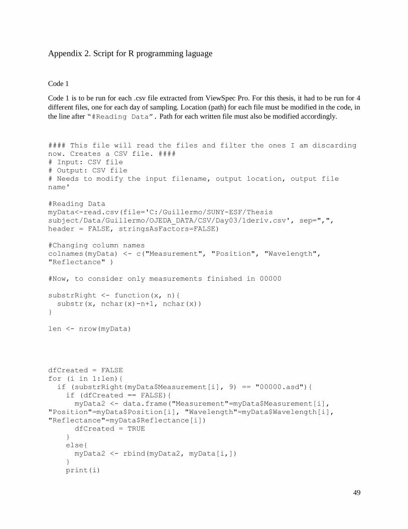
Code 1 is to be run for each .csv file extracted from ViewSpec Pro. For this thesis, it had to be run for 4

different files, one for each day of sampling. Location (path) for each file must be modified in the code, in

the line after “#Reading Data”. Path for each written file must also be modified accordingly.

#### This file will read the files and filter the ones I am discarding

now. Creates a CSV file. ####

# Input: CSV file

# Output: CSV file

# Needs to modify the input filename, output location, output file

name'

#Reading Data

myData<-read.csv(file='C:/Guillermo/SUNY-ESF/Thesis

subject/Data/Guillermo/OJEDA_DATA/CSV/Day03/1deriv.csv', sep=",",

header = FALSE, stringsAsFactors=FALSE)

#Changing column names

colnames(myData) <- c("Measurement", "Position", "Wavelength",

"Reflectance" )

#Now, to consider only measurements finished in 00000

substrRight <- function(x, n){

substr(x, nchar(x)-n+1, nchar(x))

}

len <- nrow(myData)

dfCreated = FALSE

for (i in 1:len){

if (substrRight(myData$Measurement[i], 9) == "00000.asd"){

if (dfCreated == FALSE){

myData2 <- data.frame("Measurement"=myData$Measurement[i],

"Position"=myData$Position[i], "Wavelength"=myData$Wavelength[i],

"Reflectance"=myData$Reflectance[i])

dfCreated = TRUE

}

else{

myData2 <- rbind(myData2, myData[i,])

}

print(i)

50

print('*****')

}

}

# Eliminating Red's

# myData3 <- myData2

dfCreated = FALSE

for (i in 1:nrow(myData2)){

if (substr(myData2$Measurement[i], 8,10) == "000"){

print (i)

if (dfCreated == FALSE){

myData3 <- data.frame("Measurement"=myData2$Measurement[i],

"Position"=myData2$Position[i], "Wavelength"=myData2$Wavelength[i],

"Reflectance"=myData2$Reflectance[i])

dfCreated = TRUE

}

else{

aux <- data.frame("Measurement"=myData2$Measurement[i],

"Position"=myData2$Position[i], "Wavelength"=myData2$Wavelength[i],

"Reflectance"=myData2$Reflectance[i])

myData3 <- rbind(myData3, aux)

}

#print (aux)

#print ("Added")

#print ('*****')

}

}

setwd ('C:/Guillermo/SUNY-ESF/Thesis

subject/Data/Guillermo/OJEDA_DATA/CSV/Day03/')

write.csv(myData3, file = "der1day03-filtered.csv",row.names=FALSE)

Code 2

Code 2 should run only once. Files to be read must be specified in each path location in the code.

#### This file will read the files and filter the ones I am discarding

now. Creates a CSV file. ####

# Input: CSV file

# Output: CSV file

51

# Needs to modify the input filename, output location, output file

name'

#Reading Data, now we need to set to capital first character

day00 <- read.csv(file='C:/Guillermo/SUNY-ESF/Thesis

subject/Data/Guillermo/OJEDA_DATA/CSV/Day00/Day0-filtered.csv',

sep=",", header = TRUE, stringsAsFactors=FALSE)

day00$Measurement <- gsub("p", "P", day00$Measurement)









### BUG here!!! after day 07 plants are called with CAPITAL initial.

now ALL plants gonna start with capitals.













# Next lines to add a column of zeros to each dataframe

day00 <- as.data.frame(append(day00, 0, after = 5))

colnames(day00)[5] <-"Day"




52








#Now, to create a single dataframe with all my data

allData <- rbind (day00, day01, day03, day07, day14, day21)

# And creating a CSV file with it

write.csv(allData, file = "C:/Guillermo/SUNY-ESF/Thesis

subject/Data/Guillermo/OJEDA_DATA/CSV/allDays/allData.csv",row.names=F

ALSE)

Code 3

Code 3 creates a dataframe object for R and the corresponding .csv file, in the specified path, that contains

all the collected data of interest.

## Code 03: This code will add columns according to what treatment

does the data belong

## Input: The all Data file from Code 2

## This code should have, definetily, be done by factorizing. Or was

it vectorizing?

## Known bugs: "Treatment" Does not display correctly in the summary.

Is related to datatypes,

## but I am not sure why. I think I can find a way around it.

# Reading code

myData <- read.csv(file='C:/Guillermo/SUNY-ESF/Thesis

subject/Data/Guillermo/OJEDA_DATA/CSV/allDays/allData.csv', sep=",",

header = TRUE, stringsAsFactors=FALSE)

# Eliminating the "00000.asd" ending of each name.

myData$Measurement =

substr(myData$Measurement,1,nchar(myData$Measurement)-9)

#Adding empty column called "Treatment"

53

myData = cbind(myData, Treatment='', stringsAsFactors = FALSE)

loops = nrow(myData)

#Datermining the treatment each plant belonged to, and correcting it

for (i in 1:loops){

print (i)

if (myData$Measurement[i] == "Plant01"){

myData$Treatment[i] = "Control"

}

else if (myData$Measurement[i] == "Plant02"){


}



}



}



}



}



}



}



}



}


myData$Treatment[i] = "Copper"

}



}



}



}



}

54



}



}



}



}



}

else {

myData$Treatment[i] = "Mancozeb"

}

}

write.csv(myData, file = "C:/Guillermo/SUNY-ESF/Thesis

subject/Data/Guillermo/OJEDA_DATA/CSV/allDays/allData_ver02.csv",row.n

ames=FALSE)

Code 04

Code 4 makes the statistical analysis and graphical representations. This code is not optimized and different

parts of the code should be run separately according to the graph we desire to obtain. For instance, to obtain

the graph of “Spectra” collected in one day, with the associated P-values for the F-test, do the following:

1. Run the code until the title “Plotting individually”, not including what lies below this title.

2. Run the section “Now we can do ANOVA for many wl…”, until the title “You forgot the post-hoc

test”. Remember to modify the variable “day” to represent the desired one.

3. Run the section “Plotting in a better code” until the title “Now we can do ANOVA for many wl”.

Remember to modify the variable “day” to represent the desired one.

To plot the p-values for the F-test and Tukey-HSD test, do the following:

1. Run the code until the title “Plotting individually”, not including what lies below this title.

2. Run the section “Now we can do ANOVA for many wl…”, until the title “You forgot the post-hoc

test”. Remember to modify the variable “day” to represent the desired one.

3. Run the section “You forgot the post-hoc….” until the end of the file. Remember to modify the

variable “day” to represent the desired one.

This code is not intended to work with data that does not belong to this thesis, so it may not work correctly

for other data. If anyone else is to use it, reviewing the code and adapting it to the proper end is

recommended. The author of this code will not take responsibility for any error/mistake in the code if used

by anyone else that is not him.

55

### In this code I will, finally, start creating graphs of what I

have.

### Input: file with all data, that must include the treatment that

every measurement belongs to.

### Not that the title "Measurement" was change to "Plant"

myData <- read.csv(file="C:/Guillermo/SUNY-ESF/Thesis

subject/Data/Guillermo/OJEDA_DATA/CSV/allDays/allData_ver02.csv",sep="

,", header = TRUE, stringsAsFactors=FALSE)

colnames(myData)[1] <- "Plant"

days = unique(myData$Day)

treatments = c("Control", "Copper", "Mancozeb")

plants = unique(myData$Plant)

# Vector of dataframes to be created that are the spectral data for

each plant

dfs = c()

# Create a data.frame for each PLANT and DAY that consist only of

Wavelength and Reflectance

# Chosen approach: create a function that does a subset of each plant

and transforms the corresponding df

# eval(parse(text=c))

# Have this in mind:

# eval(parse(text="print(\"hi\")"))

# This last line works OK

getSpectra <- function(plant, day){ # Gets a single spectral response

as a dataframe

# plant is a string of the list of plants,

# day is a day from the list of days

# dataframe

mySub = subset (myData, myData$Plant==plant & myData$Day==day)

df <- subset( mySub, select = -c(Plant, Day, Treatment) )

return(df)

}

# pl01d3 = getSpectra("plant01",00 ) -----> This line works!!

56

# Now, looping through every plant to create a dataframe.

# Use text substitution:

# gsub("cheap", "sheep's", "A wolf in cheap clothing")

text <- "PPdDD = getSpectra('PP',DD )"

for (i in plants){

for (j in days){

text2 <- gsub ("PP", i, text)

text3 <- gsub ("DD", j, text2)

eval(parse(text=text3))

}

}

# plant01d0 <- getSpectra('plant01', 0)

# This line works OK

# Eliminate the 2 columns of WL and Refl.

# use unique.data.frame or something like it.

spectradf <-myData [ -c(2:4) ]

spectradf <- unique.data.frame(spectradf)

subset(spectradf, Treatment=="Mancozeb" & Day==14)

######## Creating summary table #########

# Which will contain Day, Treatment, Plant, Spectra Name.

# And will be created from the data.frae "spectradf"

spectradf2<-spectradf

spectradf2$spectra <- NA

spectradf2

for (i in (1:nrow(spectradf2))){

print(i)

text1 <-spectradf2$Plant[i]

text2 <- as.character(spectradf2$Day[i])

text3 <- paste(text1,"d", text2, sep='')

spectradf2$spectra[i] <- text3

}

spectradf3 <- subset(spectradf2, Day != 21 & Day != 0)

57

plot(Plant05d7$Wavelength, Plant05d7$Reflectance, type='l', ylab =

"Reflectance", xlab="Wavelength",

col=51, ylim=c(0, 1))

write.csv(spectradf3, file = "C:/Guillermo/SUNY-ESF/Thesis

subject/Results/SpectraSummary.csv",row.names=FALSE)

# Find a way to associate each value of the created df with unique

values and the data frames created for each plant and day.

######## Plotting Individually #########

#Day 14 test# Until I can code it as a function.

plot(Plant01d14$Wavelength, Plant01d14$Reflectance, xlab="Wavelength",

ylab="Reflectance",

main = "Spectral patterns", pch=".", col = 51, type="l",

ylim=c(0, 1))

text4 <- "lines(Plant01d14$Wavelength, PlantPPdDD$Reflectance,

col=color, type = 'l')"

day=3

for (i in subset(spectradf, Treatment=="Control" & Day==day)$Plant){

plant = i

day = day

color = 51

text5 <- gsub ("PlantPP", i, text4)

text6 <- gsub ("DD", day, text5)

text7 <- gsub ("color", color, text6)


}

for (i in subset(spectradf, Treatment=="Copper" & Day==day)$Plant){

plant = i

day = day

color = "'blue'"





}

for (i in subset(spectradf, Treatment=="Mancozeb" & Day==day)$Plant){

plant = i

day = day

color = "'red'"



58



}

###### Plotting in a better code ######

treatments = c("Control", "Mancozeb", "Copper")

# Using mar() to set the margins space so I have space to write a

title of the right axis

par(mar=c(5.1,4.1,4.1,5.1)) # Default is par(mar=c(5.1,4.1,4.1,2.1))

# No need of the following line, I made a better code inseide loop.

#plot(Plant01d14$Wavelength, Plant01d14$Reflectance,

xlab="Wavelength", ylab="Reflectance",

# main = "Spectral patterns", pch=".", col = 51, type="l",

ylim=c(0,1))

text3 <- 'plot(PlantPPdDD$Wavelength, PlantPPdDD$Reflectance,

xlab="Wavelength (nm)", ylab="Reflectance (dimensionless)",

main = "Day DD", pch=".", col = 51, type="l", ylim=c(0,1))'

text4 <- "lines(Plant01d7$Wavelength, PlantPPdDD$Reflectance,

col=color, type = 'l')"

day = 14

plotDone = TRUE # Set this line to FALSE if u want to create NEW plot

axis(side=4)

mtext("P-value", side=4, line=3)

mtext("Reflectance", side=2, line=3)

for (j in treatments){

for (i in subset(spectradf, Treatment==j & Day==day)$Plant){

plant = i

day = day

if (j == "Control"){

color = 51

}

if (j == "Copper"){

color = "'blue'"

}

if (j == "Mancozeb"){

color = "'red'"

59

}




if (plotDone == FALSE){





axis(side=4)

mtext("P-value", side=4, line=3)

plotDone <- TRUE

}

else{


}

}

}

legend("topright", inset=0.04, legend=c("Mancozeb", "Copper",

"Control", "P-values"),

col=c("red", "blue", "Green", "black"), lty=c(1, 1, 1, NA),

pch=c(NA, NA, NA, "o"), cex=1)

abline (h=0.05, col="red", lty="dotted")

# abline (h=0.10, col="red", lty="dotdash")

# abline (h=0.20, col="red")

# These last 3 lines add the lines for alpha values of 5%, 10% and 20%

###### Now, carefully, we will do anova ########

# Need to choose a day, cause we are doing by DAY

# Setting a DF for only 1 day, called mydf

mydf <- subset(myData, Day == 3)

# Need to choose wavelength first!!!

wl = 1930

# Selecting only the WL of interest

mydf2 <- subset(mydf, Wavelength == wl)

# Performing ANOVA

results <- aov (Reflectance ~ Treatment, data = mydf2)

summary(results)

60

###### Now, we can do ANOVA for many WL. For example, all of them in

the same day #######

day = 14

mydf <- subset (myData, myData$Day == day)

wl = unique(mydf$Wavelength)

# Example

#12 %in% 10:20

#[1] TRUE

resultsdf <- data.frame ("Wavelength"=1100, "Pvalue"=0.3) #Initialize

first row

colnames(resultsdf) <- c("Wavelength", "Pvalue")

counter <- 0

for (i in wl){

if (i %in% wl){

counter <- counter +1

mydf2 <- subset(mydf, Wavelength == i)


toAdd <- c(i, summary(results)[[1]][["Pr(>F)"]]) # The second

component is the P value of the current ANOVA

print(toAdd)

resultsdf <- rbind(resultsdf, toAdd)

}

}

resultsdf <-resultsdf[-1,] #Delete first row

sortedResults <- resultsdf[order(resultsdf$Pvalue),] # This DF sorts

the previous one according ascending P-value

sortedResults [1:20,] #This line to get best 20 lines... Useless

because of high correlation

sortedResults

#summary(test)[[1]][["Pr(>F)"]]

par(mar=c(5.1,4.1,4.1,5.1)) # Default is par(mar=c(5.1,4.1,4.1,2.1)) #

This line sets margins size

plot(sortedResults$Wavelength, sortedResults$Pvalue, ylim=c(0,1),

xlab="Wavelength(nm)", ylab="Reflectance") # Pay attention to this

61

write.csv(sortedResults, file = "C:/Guillermo/SUNY-ESF/Thesis

subject/Results/Day01AnovaPower.csv",row.names=FALSE)

########## You forgot the POST HOC TEST, !!!!!!!!!!! ############

########## Doing it now! ############

# Example: Use this to get a p value for a given treavtment vs

treatment p value:

# tuk<- TukeyHSD(results)

# tuk2<-tuk[1]$Treatment

# tuk2[10] # This for Copper vs Control

# tuk2[11] # This for Mancozeb vs Control

# tuk2[12] # This for Mancozeb vs Copper

# Do this for each band!!!! Implement in the previous loop (loop taken

and modified from the previous one,

# where I was only Doing ANOVA)

day = 14

mydf = mydf <- subset (myData, Day == day)

wl = unique(mydf$Wavelength)

# Example

#12 %in% 10:20

#[1] TRUE

resultsdf <- data.frame ("Wavelength"=1100, "Pvalue"=0.92, "Copper-

Control"=0.3, "Mancozeb-Control"=0.3, "Mancozeb-Copper"=0.3)

colnames(resultsdf) <- c("Wavelength", "Pvalue", "Copper-Control",

"Mancozeb-Control", "Mancozeb-Copper")

counter <- 0

for (i in wl){

if (i %in% wl){

counter <- counter +1

mydf2 <- subset(mydf, Wavelength == i)


tuk<- TukeyHSD(results)

tuk2<-tuk[1]$Treatment

copCon <- tuk2[10] # This for Copper vs Control

manCon <- tuk2[11] # This for Mancozeb vs Control

manCop <- tuk2[12] # This for Mancozeb vs Copper

toAdd <- c(i, summary(results)[[1]][["Pr(>F)"]][1], copCon,

manCon, manCop ) # The second component is the P value of the current

ANOVA

print(toAdd)

62

resultsdf <- rbind(resultsdf, toAdd)

}

}

resultsdf <- resultsdf[-1,]

sortedResults <- resultsdf[order(resultsdf$Pvalue),] # This DF sorts

the previous one according ascending P-value

sortedResults [1:20,] #This line to get best 20 lines... Useless

because of high correlation

sortedResults

#summary(test)[[1]][["Pr(>F)"]]

plot(resultsdf$Wavelength, resultsdf$Pvalue, xlab="Wavelength (nm)",

ylab = "P-Value for Tukey HSD", ylim=c(0,1))

# Now, adding Tukey's result

points(resultsdf$Wavelength, resultsdf$`Copper-Control`, col = 'Blue',

type ="l")

points(resultsdf$Wavelength, resultsdf$`Mancozeb-Control`, col =

'Red', type = 'l')

abline(h=0.05, lty = 'dotted', col = 'red')

legend("top", inset=0.02, legend=c("Mancozeb vs. Control", "Copper vs.

Control", "P-values"),

col=c("red", "blue", "black"), lty=c(1, 1, NA), pch=c(NA,

NA,"o"), cex=1)

##points(resultsdf$Wavelength, resultsdf$`Mancozeb-Copper`, col =

'Yellow')

## Las lilne uncommented because it was suggested not to plot Cooper

vs Mancozeb.

write.csv(sortedResults, file = "C:/Guillermo/SUNY-ESF/Thesis

subject/Results/Day14AnovaPower.csv",row.names=FALSE)

63

Vita

Guillermo Francisco Ojeda

Education

Master of Sciences on Environmental Engineering Expected: May 2019 State University of New York – College of Environmental Sciences and Forestry (SUNY-ESF)

Syracuse, New York.

GPA: 3.58

Agriculture Engineer May 2009

School of Agrarian Sciences - Cuyo National University. Mendoza, Argentina

GPA: 7.56 out of 10.00

Work Experience

Field Engineer at Grupo Bioprocesos: Mendoza, Argentina. May 2012 to July 2017 Department of Environmental Engineering, School of Engineering, Cuyo National University.

• Study of pollution and industrial activities impact in different provinces of Argentina.

• Environmental characterizations: project managing, schedule planning, team direction, study of the industrial activities and their impact in the society and environment.

• Underground water monitoring, study of cases and follow-up over time

• Use of Geographic Information Systems software to perform geoprocessing tasks, elaborate

cartography, predict future situations based in corresponding models.

• Biological remediation of soils contaminated with hydrocarbons.

• Protocols elaboration, laboratory tasks, elaborating reports.

Technical assistant at ISCAMEN: Mendoza, Argentina. March 2012 - May 2012 ISCAMEN (Institute of Agriculture Quality and Sanitation of Mendoza)

• Sanitary inspections in different commercial establishments in the province of Mendoza,

Argentina, as part of the corresponding inspections team.

• Database administration and maintenance regarding to the use of pesticides in the province of

Mendoza

• Extension and instruction to third parties regarding use of pesticides and safety concerns. Technical assistant at INTA EEA Mendoza Mendoza, Argentina June 2011 – February 2012

Technical Assistant, Norton Winery Mendoza, Argentina January 2011 - May 2012

Intern, Beaulieu Vineyards winery, Rutherford, California. August 2010 – December 2010 Intern, Peñaflor winery, Mendoza, Argentina January 2011 - July 2011

Intern, “El Poniente” Winery, Mendoza, Argentina February 2008 – April 2008

Intern, “El Poniente” Winery, Mendoza, Argentina June 2008 – November 2008

Documents

Evaluation of the Spectral Reflectance Pattern of Capsicum