COMPENDIUM OF RESEARCH ACTIVITIES TO DATE: EVALUATION OF THE PERFORMANCE OF TEXAS ASPHALT CONCRETE

PAVEMENTS MADE WITH DIFFERENT COARSE AGGREGATES

B. F. McCullough

D. G. Zollinger

Research Compendium 1244-2 (Vol. 2)

Evaluation of the Performance of Texas Pavements Made with Different Coarse Aggregates Research Project 213- 12D-9014- 1244

conducted for the

Texas Department of Transportation

in cooperation with the

U.S. Department of Transportation

Federal Highway Administration

by the

CENTER FOR TRANSPORTATION RESEARCH

Bureau of Engineering Research

THE UNIVERSITY OF TEXAS AT AUSTIN

and the

TEXAS TRANSPORTATION INSTITUTE

TEXAS A&M UNTVERSITY

May 1993

Study Supervisor: Dr. B. F. McCullough, P.E. (Texas No. 19914)

The contents of this report reflect the view of the authors, who are responsible for the

facts and the accuracy of the data presented herein. The contents do not necessarily reflect the

official views or policies of the Federal Highway Administration or the Texas Department of

Transportation. This report does not constitute a standard, specification, or regulation.

PREFACE

This is the Compendium of Information (Volume 2) "Evaluation of the

Performance of Texas Asphalt Concrete Pavements made with Different Coarse

Aggregates." This compendium is summarized by the fifth report for Research Project

1244, "Preliminary Research Findings on the Affect of Coarse Aggregate on the

Performance of Portland Cement Concrete Paving." This compendium of information

was the result of a joint effort between the University of Texas at Austin, Center for

Transportation Research and the Texas Transportation Institute.

In this compendium, the various areas of research that have been performed to

date on aggregates used for both asphalt and Portland Cement Concrete pavements are

documented. Field and laboratory investigations have shown that significantly different

pavement performance con be expected for aggregates with relatively high thermal

coefficients. With regard to concrete pavements, environmental conditions at the time of

placement have also been closely tied to performance.

We would like to thank the staff of the Texas Department of Transportation for

their support throughout this study. Their interest and enthusiasm in this project has

resulted in numerous pavement test sections being constructed in Houston, LaPorte,

Cypress, and Texarkana, Texas. These well documented test sections will provide

Department engineers with excellent data on the long term performance of pavements

constructed with different aggregates.

iii

ABSTRACT

For many years, engineers have recognized the different performance

characteristics of asphalt and concrete pavements constructed with different coarse and

fine aggregates. Past research has shown the importance of monitoring these aggregates

for physical and chemical properties such as abrasion resistance, polish value, gradation,

soundness, fineness modulus, specific gravity, and absorption. Using various tests to

determine these aggregate properties, engineers are able to screen aggregates before they

are ever used for pavement construction. Unfortunately, this selection of tests does not

insure the long term performance of pavements in the field as illustrated by the numerous

pavement failures at early age. This research attempts to address these shortfalls in the

quality control and pavement design processes related to aggregates used in construction. This research has been comprehensive in the area of pavement aggregate. Numerous

Master's Thesis' and Ph.D. dissertations have been completed under the auspices of this

study. These include work performed both at Texas A & M University and the

University of Texas at Austin. As a result, the principal investigators responsible for this

study, felt it was necessary to pull together all of the work that has been performed to date in the form of a compendium. The compendium is comprehensive and includes detailed

research activities that have been conducted to date.

SUMMARY

This compendium of information presents all of the research activities that have

been completed to date for this study. This compendium of information is meant to

illustrate the many of the research activities that have been completed to date both at

Texas A & M University and the University of Texas at Austin. The compendium of

information focuses on research activities related to aggregates used in the construction of

asphalt concrete pavements.

This compendium of information also addresses research activities related to

aggregates used in the construction of Portland cement concrete pavements. These

include specific chapters addressing topics such as field investigations of spalling and

punch-out distresses in continuously reinforced and jointed pavements, aggregate shape

characterization using fractals, and determination of saw-cut depth using fracture

analysis. Some of these activities relate directly to improving pavement performance regardless of aggregate type used for construction.

Work to date has also focused on identifying significant factors that affect the

performance of asphalt and concrete pavements. Significant accomplishments have been

made in this area and early recommendations have been made to the Texas Department of

Transportation regarding implementation of these findings. The details of these

recommendations are documented in another 1244 report regarding field implementation

of significant findings, to be published at a later date.

IMPLEMENTATION STATEMENT

The findings discussed within this report will help optimize designs of Portland cement

concrete pavements. Improvements in coarse aggregate selection can, by offsetting various

distress manifestations, lead to improved pavement performance. The field data collected and

evaluated in this report can also potentially serve as the basis for improving existing design

equations. These equations take into consideration the studies on determination of saw-cut depth

using fractal analysis. Finally, improvement in material selection for pavement construction can

translate into a direct cost benefit to the Department.

TABLE OF CONTENTS - VOLUME I1

. . Preface.. ............................................................................................ 11

Abstract ............................................................................................. iii

Summary.. ......................................................................................... iv

Implementation Statement ........................................................................ v

CHAFlTR 1: INTRODUCTION AND BACKGROUND 1.1 Origination of Problem Statement

1.2 Study Objectives and Overview of Project Work Plan

CHAPTER 2: FIELD INVESTIGATIONS ON SPALLING OF CRCP AND JCP

2.1 Pavement Spalling

2.2 Field Investigations

2.3 Summary of Field Investigations

2.4 Causes and Mechanisms

2.5 References

CHAPTER 3: BASIC FAILURE MODES LEADING TO PUNCHOUT DISTRESS IN CRC PAVEMENT

3.1 Basic Failure Modes

3.2 Spall Development and Analysis

3.3 References

CHAPTER 4: CRACK CONTROL METHODOLOGIES FOR CRCP AND JCP

CHAPTER 5: AGGREGATE SHAP AND CHARICI'ERIATION WITH FRACTALS 5.1 Background and Introduction

5.2 Objective of the Research Tasks

5.3 Discription of Analysis k e d u r e 5.4 Discussion of Results

5.5 Recommendation for Future Research

5.6 References

CHAPTER 6: EVALUATION OF COARSE AGGREGATES ON PCC FRACIWRE ANALYSIS

6.1 Introduction

6.2 Basic Concepts of Linear Elastic Fracture Mechanics

6.3 Nonlinear Fracture Mechanics of Concrete

6.4 Methods for Deterrninization of Fracture Parameters

6.5 Specimans

6.6 Fracture Tests and Results

6.7 References

CHAPTER 7: DETERMINATION OF SAWCUT DEPTH AND SPACING WITH

FRACTURE ANALYSIS

7.1 Introduction

7.2 Theoretical Approach: Climatic Stresses

7.3 Calculation of Climatic Stresses

7.4 Sawcut Spacing Depth Requirements

7.5 Theory and Application of Fracture Mechanics

7.6 Effects of Pavement Thickness on the Sawcut Depth

7.7 Field Investigation of Crack Control

7.8 Conclusions

7.9 References

CHAPTER 8: ANALYSIS OF CONCAVE CURLING IN CONCRETE SLABS

8.1 Introduction

8.2 Basic Equations

8.3 Stresses In An Infiite Pavement

8.4 Stresses In A Semi-Infiiite Pavement

8.5 Stresses In An Infinitely Long Pavement With A Finite Width

8.6 Maximum Stress In A Finite Pavement

8.7 Conclusions

8.8 AppendixI.

8.9 Appendix I1 8.1 0 Appendix

CHAPTER 9: TOW-DIMENTIONAL ANALYSIS OF CRCP AT EARLY AGES

9.1 The Stress Modle

9.2 Drying Shrinkage Model

9.3 Nodal Strain Loading

9.4 Creep Model 9.5 Bond Slip Modeling

9.6 Analysis and Results

9.7 Shrinkage Strain Prediction

9.8 References

CHAF'TER 10: CONCLUSIONS AND RECOMMENDATIONS

10.1 Literature Review and Field Investigations on PCC Pavements

10.2 Crack Control Methods Reposes for PCC Pavements

10.3 Characterization of Aggreagate Texture and Shape With Fractals

10.4 Aggregate Effects on Fracture Properties of Portland Cement Concrete

10.5 Fracture Analysis on PCC Pavement Saw-Cut Depth and Spacing Requirements

10.6 Analysis of Thermal Stresses in Concave Curled Concrete Slabs

10.7 Two-Dimentional Analysis if CRC Pavement at Early Ages

viii

CHAPTER 1

INTRODUCTION

1.1 BACKGROUND

In Texas, it has been customary for contractors involved in the construction of both

asphaltic concrete (AC) and portland cement concrete (PCC) pavements to discount the variation

in pavement material properties that results from the use of different coarse aggregate types in

the pavement mix. But as studies show, such practice not only compromises pavement

performance, it also perpetuates a broader misunderstanding of the coarse aggregate has on

pavement performance. In this study, a substantial effort has been made to document the effects

coarse aggregate has on such pavement parameters as modulus of elasticity, thermal expansion

coefficient, mortar/aggregate bonding characteristics, and tensile strength.

As previous research has demonstrated, the type of aggregate used in a pavement mix can

significantly increase the likelihood of a particular pavement distress being observed. In the

particular case of PCC pavements -- principally continuously reinforced concrete (CRC)

pavements -- the effects of different coarse aggregates can contribute to irregular cracking

patterns which, in turn, can lead to punchouts, spalling, and undesirable crack intervals. In the

case of asphalt pavements, the use of various aggregates can result in surface rutting (caused

primarily by the progressive movement of materials under repeated loads, either in the pavement

layers and/or in the underlying base of subgrade).

Under present Texas specifications, the actual selection of the coarse aggregate used

during construction of, for example, CRC pavement is left to contractors. Engineers who write ,. these specifications usually assume that, as long as the contractor's proposed aggregate meets the

basic gradation and physical requirements, the aggregate will perform adequately. It is during

the competitive bidding process that the contractor generally selects the aggregate type, with that

decision based primarily on competitive prices received from the various aggregate suppliers,

most of whom operate near the construction site. The pavement specified in the construction

documents is then constructed with the -least expensive coarse aggregate that still meets the

state's quality control specifications -- in spite of a n increasing variety of specialty coarse

aggregate types becoming available for paving in Texas today. The consequence is that most of

the pavements are constructed with materials using either (1) a crushed limestone aggregate of

(2) a siliceous river gravel.

I 1.2 OBJECTIVES

This study will focus primarily on the effect of the coarse aggregate on the performance

of CRC, jointed concrete pavement, and hot-mix asphalt concrete (HMAC) pavement. Various

distresses in these types of pavements have been selected for smc research into their

associative causes, in an effort to determine corrective measures. These measures are characterized by the type of coarse aggregate used in the pavement (either concrete of asphalt).

The specific objectives of this study include the following:

1. To collect and analyze information available from field and laboratory evaluations that

may lead to the description and explanation to the effects a coarse aggregate type may have on

the performance of AC and PCC pavements in Texas.

2. To identify and focus on significant pavement distresses, determining how the failure

modes and the distress manifestations are related to the types and physical characteristics of

aggregates used in Texas.

3. To develop model improvements to account for aggregate-related distresses not presently

accounted for.

4. To propose alternative design andlor construction methods (with industry input) that

reduce identified pavement distress and that improve pavement performance. These methods

will involve practical-solution approaches that can be implemented by TxDOT.

13 SCOPE OF REPORT

The project was divided into three phases: afield phase, a laboratory phase, and a design-

model improvement phase. The field and laboratory phases of this study were designed to

determine relationships between coarse aggregate characteristics and specific modes of pavement

distress related to pavement cracking, spalling, and rutting. Specifically, the field investigation,

described in Chapter 3 and following the literature review reported in Chapter 2, included (1)

investigating specific pavement distress as a function of the coarse aggregate type, and (2)

examining existing asphalt and concrete pavement sections comprised of different aggregate

types. The first area of emphasis considers as a minimum the coarse aggregate factors affecting

the development of spalling in CRC (and jointed if applicable) pavement, and rutting in asphalt

concrete pavement. (Here it should be understood that the influence of the coarse aggregate in

asphalt concrete pavement cannot be completely isolated fkom the often ovemding effects of the

fine aggregate and the size of the filler particles.)

The laboratory program, also described in Chapter 3, involved experiments conducted

with both concrete and asphalt pavements to verify findings from the field study -- findings used

in the fmal phase to modify the design guidelines in terms of aggregate characteristics. The

concrete laboratory work provides verification data for relationships between concrete

mechanical characteristics, environmental conditions, and the time of construction. The asphalt

laboratory work, however, again presented certain limitations. There are presently no standard

tests of materials specifications that directly address asphalt aggregate properties (e.g., particle

shape and surface texture). It is well known, however, that these properties directly affect

asphalt concrete pavement performance, with mixture tests, including Hveem stability and axial

compression, providing an indirect measure of these aggregate qualities. Yet the relatively high

incidence of pavement failure, which often appears related to deficient aggregate quality,

indicates that there is a need both to develop test methods and to establish acceptance criteria that

can be used to identifv these substandard aggregates.

Finally, the design-model improvement phase of this report, documented in Chapter 4,

describes modifications made to enhance both the CRC and the AC model. Additionally, this

phase addresses the economic implications of the design aspects based on a consideration of the

coarse aggregate effects for both asphalt and concrete pavements, and the discuss the field

implementation of the most promising crack induction and design techniques developed under

this and other studies for both asphalt and concrete pavements.

This work is believed to be significant in that it addresses the issue of achievingh Texas

equal pavement performance using different coarse aggregates in state pavement construction. It

comes partly in response to a new design procedure issued by TxDOT Highway Design Division

in 1981 that called for more rational analysis of all the factors influencing CRC pavement

performance -- that design procedure itself a revision based on the findings recommended in

Report 177-22F. "Summary and Recommendations for the Implementation of Rigid Pavement

Design, Construction, and Rehabilitation Techniques (Year?)."

In pursuing the objectives of this project, the study team organized field data and

conducted analyses based on techniques that permit conclusions regarding the practical

performance differences of various aggregates used in Texas for pavement construction. The

results of this investigation should, when implemented, yield pavements that perform uniformly

well, irrespective of the material used in their design. Because of the long-range implications and scope of this study, both the Center for Transportation Research (m) at The University of Texas at Austin and the Texas Transportation Institute (TTI) at Texas A&M University participated in this project.

CHAPTER 2

FIELD INVESTIGATIONS ON SPALLING OF CRCP AND JCP

2.1 PAVEMENT SPALLING

Spalling in concrete pavements has been a problem faced by pavements engineers for a

long time. It increases roughness in the pavement causing it to have reduced serviceability and

safety. More importantly, it reduces the load transfer efficiency across joints or cracks, which

leads to higher stresses in the pavement slab. However, published literature does not carry much

information on this very important topic.

Spalling can occur in both jointed concrete pavements (JCP) and continuously reinforced

concrete pavements (CRCP). In JCP, spalling can occur in the form of joint spdling or comer

spalling, whereas in CRCP, spalling would primarily occur at the transverse cracks. Zollinger and

Barenberg (1990) defined spalling of continuously reinforced concrete pavements as the

breakdown of the pavement along the cracks leading to the loss of concrete and the disintegration

of the load transfer mechanism.

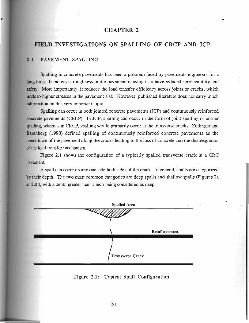
Figure 2.1 shows the configuration of a typically spalled transverse crack in a CRC

pavement.

A spall can occur on any one side both sides of the crack. In general, spalls are categorized

by their depth. The two most common categories are deep spalls and shallow spalls (Figures 2a

and 2b), with a depth greater than 1 inch being considered as deep.

Spalled Area

\ Reinforcement

Figure 2.1: Typical Spall Configuration

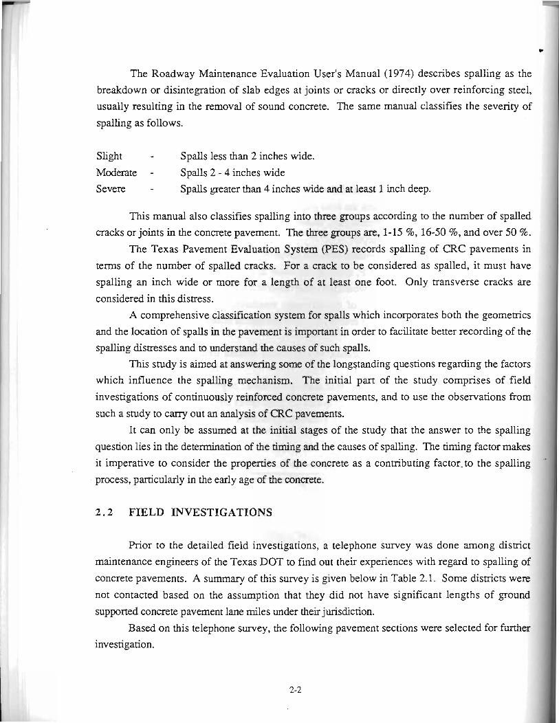
The Roadway Maintenance Evaluation User's Manual (1974) describes spalling as the

breakdown or disintegration of slab edges at joints or cracks or directly over reinforcing steel,

usually resulting in the removal of sound concrete. The same manual classifies the severity of

spalling as follows.

Slight - Spalls less than 2 inches wide.

Moderate - Spalls 2 - 4 inches wide

Severe - Spalls greater than 4 inches wide and at least 1 inch deep.

This manual also classifies spalling into three groups according to the number of spalled

cracks or joints in the concrete pavement. The three groups are, 1-15 %, 16-50 %, and over 50 %.

The Texas Pavement Evaluation System (PES) records spalling of CRC pavements in

terms of the number of spalled cracks. For a crack to be considered as spalled, it must have

spalling an inch wide or more for a length of at least one foot. Only transverse cracks are

considered in this distress.

A comprehensive classification system for spalls which incorporates both the geomemcs

and the location of spalls in the pavement is important in order to facilitate better recording of the spalling distresses and to understand the causes of such spalls.

This study is aimed at answering some of the longstanding questions regarding the factors

which influence the spalling mechanism. The initial part of the study comprises of field

investigations of continuously reinforced concrete pavements, and to use the observations from

such a study to cany out an analysis of CRC pavements.

It can only be assumed at the initial stages of the study that the answer to the spalling

question lies in the determination of the timing and the causes of spalling. The timing factor makes

it imperative to consider the properties of the concrete as a contributing factor-to the spalling

process, particularly in the early age of the concrete.

2.2 FIELD INVESTIGATIONS

Prior to the detailed field investigations, a telephone survey was done among district

maintenance engineers of the Texas DOT to find out their experiences with regard to spalling of

concrete pavements. A summary of this survey is given below in Table 2.1. Some districts were

not contacted based on the assumption that they did not have significant lengths of ground

supported concrete pavement lane miles under their jurisdiction.

Based on this telephone survey, the following pavement sections were selected for further investigation.

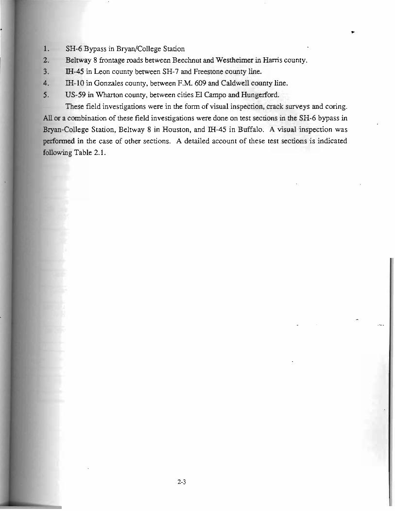
1. SH-6 Bypass in BrydCollege Station 2. Beltway 8 frontage roads between Beechnut and Westheimer in Harris county.

3. IH-45 in Leon county between SH-7 and Freestone county line.

4. M-10 in Gonzales county, between F.M. 609 and Caldwell county line.

5 . US-59 in Wharton county, between cities El Campo and Hungerford.

These field investigations were in the form of visual inspection, crack surveys and coring.

All or a combination of these field investigations were done on test sections in the SH-6 bypass in Bryan-College Station, Beltway 8 in Houston, and M-45 in Buffalo. A visual inspection was

performed in the case of other sections. A detailed account of these test sections is indicated

following Table 2.1.

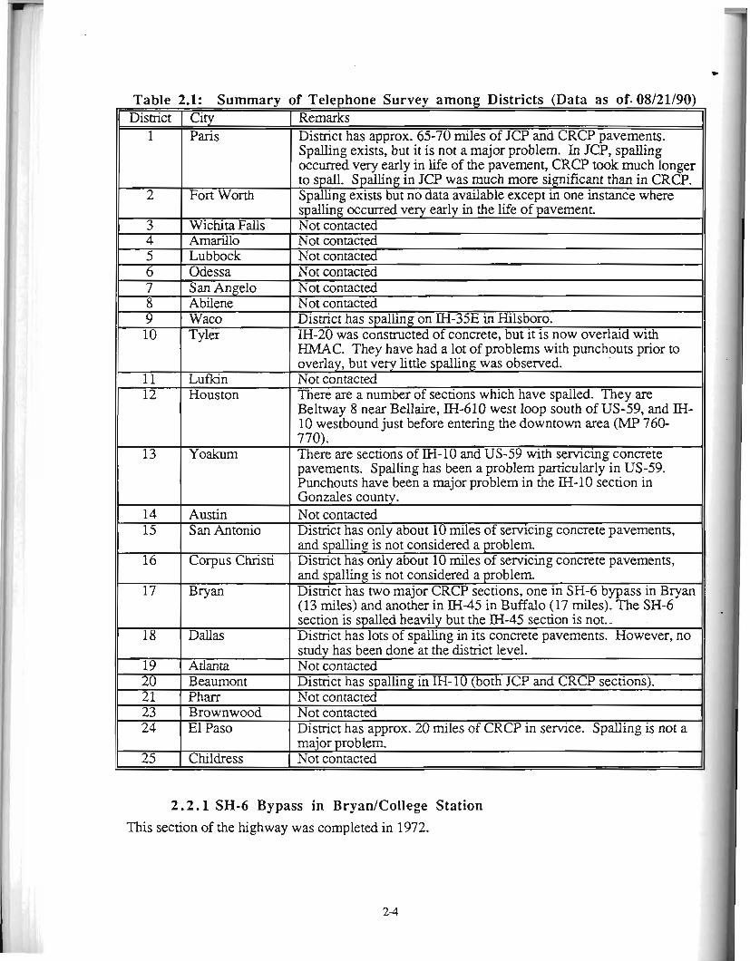
Table 2.1: Summary of Telephone Survey among Districts (Data as of- 08/21/90)

3 4 5 6 7 8 9 10

Remarks District has approx. 65-70 miles of JCP and CRCP pavements. SpaUing exists, but it is not a major problem. In JCP, spalling occurred very early in life of the pavement, CRCP took much longer to spdl. Spalling in JCP was much more significant than in CRCP. S~allinn exists but no data available except in one instance where

District 1

2

-- -

11 12

City Paris

Fort Worth

Wichita Falls Amarillo Lubbock Odessa San Angelo Abilene Wac0 Tvler

13

14 15

s ~ a l l i n ~ c u r r e d very early in the life ofpavement. Not contacted Not contacted Not contacted Not contacted Not contacted Not contacted Disbict has spalling on IH-35E in Hilsboro. IH-20 was constructed of concrete, but it is now overlaid with .

4 -

Luflan Houston

1

HMAC. They have had a lot of problems with punchouts prior to overlay, but very little spalling was observed. Not contacted There are a number of sections which have spalled. They are Beltway 8 near Bellaire, IH-610 west loop south of US-59, and M- 10 westbound just before entering the downtown area (MP 760-

Yoakum

Austin S an Antonio

17

770). There are sections of M-10 and US-59 with servicing concrete pavements. Spalling has been a problem particularly in US-59. Punchouts have been a major problem in the IH-10 section in Gonzales county. Not contacted District has only about 10 miles of servicing concrete pavements,

16

I Bryan

19 20 2 1 23 24

2.2.1 SH-6 Bypass in BryanlCollege Station This section of the highway was completed in 1972.

Corpus Christi and spalling is not considered a problem District has two major CRCP sections, one in SH-6 bypass in Bryan (13 miles) and another in M-45 in Buffalo (17 miles). The SH-6

18

25

and spalling is not considered a problem. District has only about 10 miles of senicing concrete pavements,

( section is.spalled heavily but the IH-45 section is not.- Dallas 1 District has lots of suallinn in its concrete pavements. However, no

Atlanta Beaumont Pharr Brownwood El Paso

study has been done'at thgdistrict level. Not contacted Dismct has spalling in IH-10 (both JCP and CRCP sections). Not contacted Not contacted District has approx. 20 miles of CRCP in service. Spalling is not a

Childress major problem. Not contacted

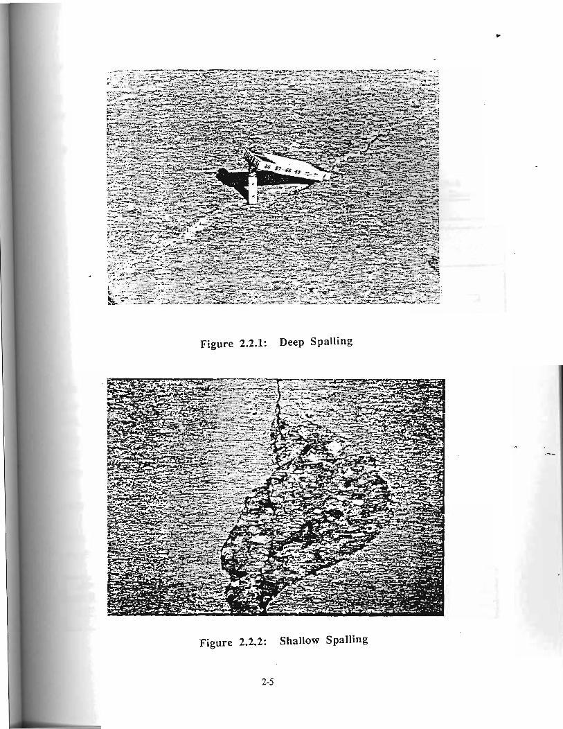
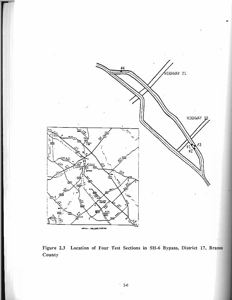
Figure 2.3 Location of Four Test Sections in SH-6 Bypass, District 17, Brazos County

Location :

The test sections are located in the east bypass of SH-6 in the Bryan-College Station area.

Figure 2.3 indicates the location of the four test sections. Each section was 200 ft. long.

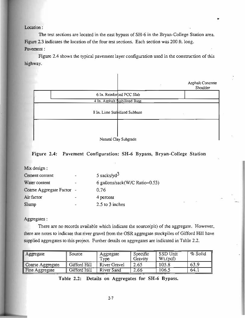
Pavement :

Figure 2.4 shows the typical pavement layer configuration used in the construction of this

highway.

I Asphalt Concrete Shoulder

4 In. As~halt Stabilized Base 1

8 In. Lime Stal~ilized Subbase

I Natural clay Subgrade I

Figure 2.4: Pavement Configuration: SH-6 Bypass, Bryan-College Station

Mix design :

Cement content - 5 sackdyd3

Water content - 6 gallons/sack(W/C Ratio=0.53)

Coarse Aggregate Factor - 0.76 Air factor - 4 percent

Slump - 2.5 to 3 inches

Aggregates :

There are no records available which indicate the source(pit) of the aggregate. However,

there are notes to indicate that river gravel from the OSR aggregate stockpiles of Gifford Hill have

supplied aggregates to this project. Further details on aggregates are indicated in Table 2.2.

f%gregate Source Aggregate Specific SSD Unit % Solid Type Gravity W t. (pcf)

Coarse Aggregate Gifford Hill River Gravel 2.65 105.8 63.9 Fine A ate 7 Gifford Hill River Sand 2.66 106.5 64.1

Table 2.2: Details on Aggregates for SH-6 Bypass.

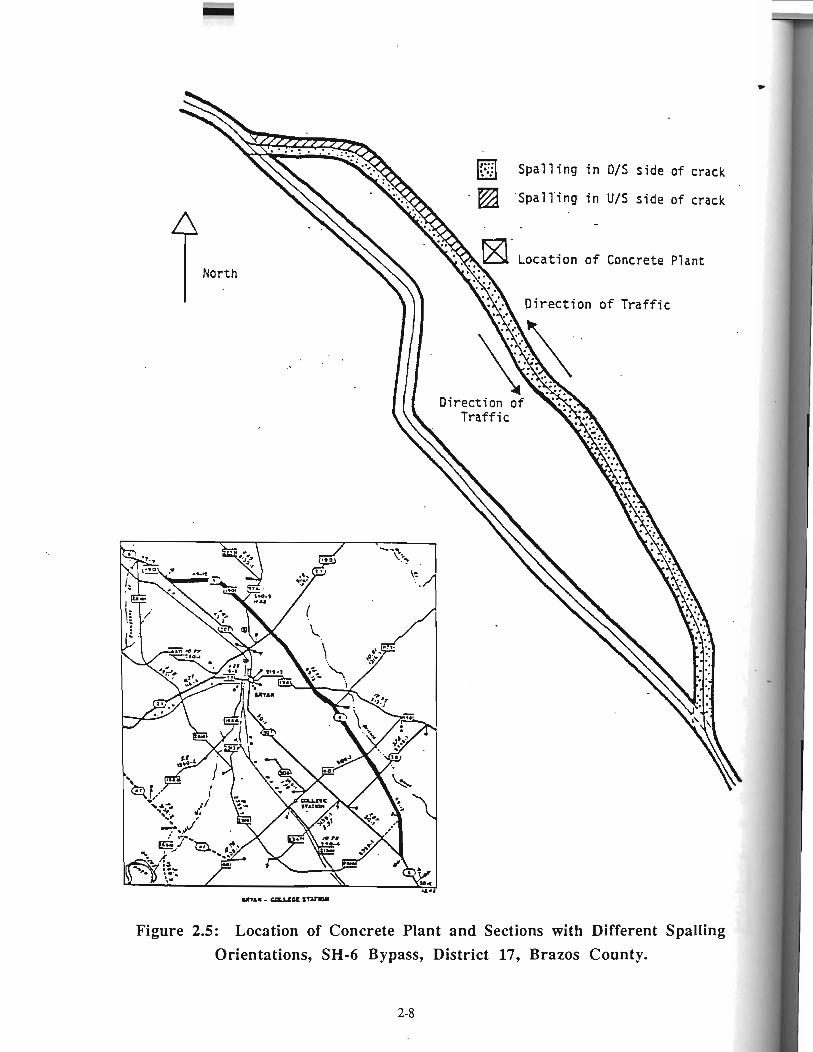
7 - North

Figure 2.5: Location of Concrete Plant and Sections with Different Spalling Orientations, SH-6 Bypass, District 17, Brazos County.

* Other Information : Cement - Gifford Hill Company, Dallas.

Water - City of Bryan

Construction:

39 Nos. 5/8" ribbed steel bars were used as longitudinal reinforcement. Transverse steel

was 112" dia. bars @ 24 in. intervals. Pavement was laid using slip-form construction and all 24

ft. of width was laid in one run. Membrane curing was used. Burlap sack drag was used for the

SU r >-

lo definite information was available on the paving sequence of this test section.

However, Texas DOT sources involved in the construction of the bypass indicated that the concrete

plant was located very close to the intersection between the SH-6 Bypass and SH-21. This may

hav~ :thing to do with the fact that the spalls are oriented differently on each side of SH-21

nm d. Figure 2.5 indicates the location of the concrete plant and the areas of the bypass with

different spa11 orientations.

No information on the paving of the bypass could be located at the district office in Bryan.

If this information were available, it would have been very important to establish a possible link

between the direction of pavingltraffic flow and the orientation of the spalls at a transverse crack.

e some

hbounc

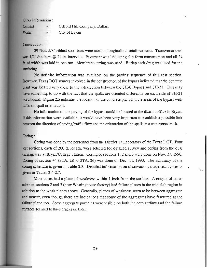
Coring :

Coring was done by the personnel from the Dismct 17 Laboratory of the Texas DOT. Four

test sections, each of 200 ft. length, were selected for detailed survey and coring from the dual

caniageway at Bryan/College Station. Coring of sections 1 ,2 and 3 were done on Nov. 27, 1990.

Coring of section #4 (STA. 28 to STA. 26) was done on Dec. 11, 1990. The summary of the

coring schedule is given in Table 2.3. Detailed information on observations made from cores is ..

given in Tables 2.4-2.7.

Most cores had a plane of weakness within 1 inch from the surface. A couple of cores

taken at sections 2 and 3 (near Westinghouse factory) had failure planes in the mid slab region in

addition to the weak planes above. Generally, planes of weakness seem to be between aggregate

and mortar, even though there are indications that some of the aggregates have fractured at the

failure plane too. Some aggregate particles were visible on both the core surface and the failure

surfaces seemed to have cracks on them.

Section Number Direction Starting Station Ending No. of Cores Taken Number Station Number

7

1 Southward 529 53 1 4 (#I-#4) 2 Southward 589 59 1 6 (#5-1-#9) 3 Northward 586 5 84 5 (#101-#105) 4 Northward 28 26 6 (#20 1 -#206)

Table 2.3: Summary of Coring Schedule. 1 Outside

2 1 530+ Outside

I

3 1 529+ Inside

4 1 5 30+ Inside

I I I

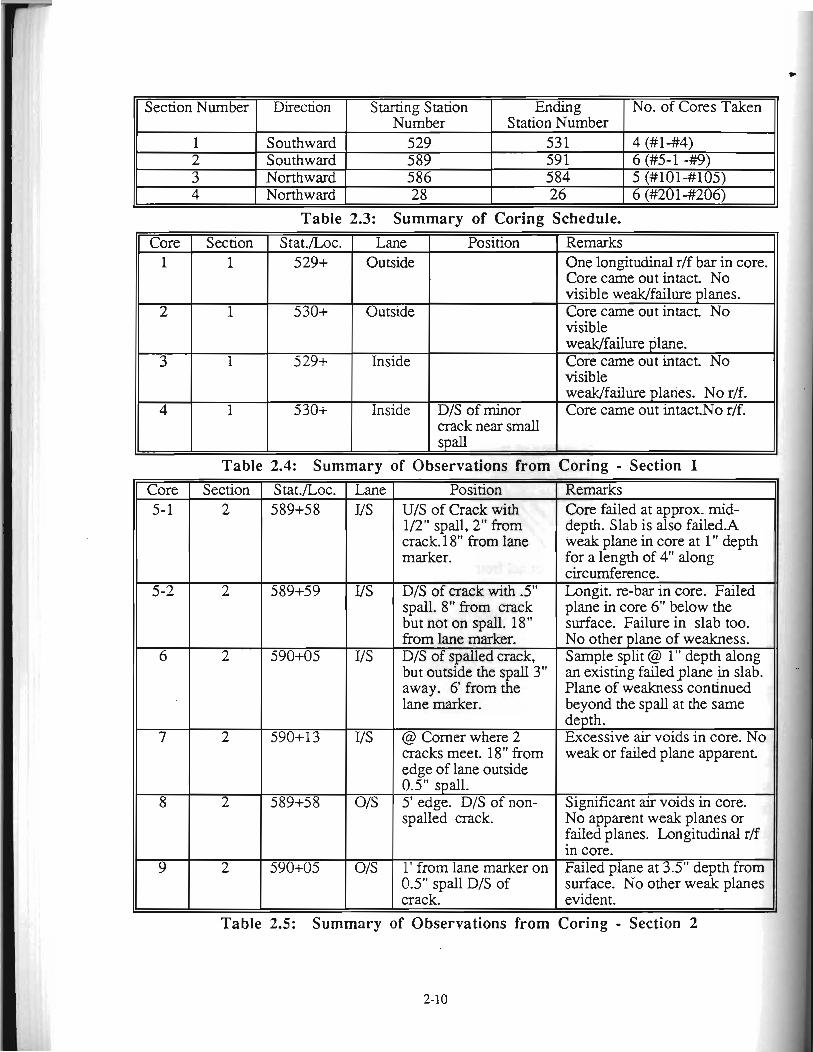
Table 2.4: Summary of 0

Position

D/S of minor crack near small spall

~servations from Position

U/S of Crack with 112" spall, 2" from crack 1 8" from lane marker.

DIS of crack with .5" spall. 8" from crack but not on spall. 18" from lane &ker. D/S of spalled crack, but outside the spall3" away. 6 from the lane marker.

@ Comer where 2 cracks meet. 18" from edge of lane outside 0.9' spall.

1 5' edge. DIS of non- spallid crack.

1' from lane marker on 0.5" spall D/S of

Remarks One longitudinal rlf bar in core. Core came out intact No visible weaklfailure planes. Core came out intact. No visible weaklfailure plane. Core came out intact No visible weaklfailure plaries. No rlf. Core came out intactNo rlf.

Coring - Section 1

Core failed at approx. mid- depth. Slab is also fai1ed.A weak plane in core at 1" depth for a length of 4" along circumference. Lonnit. re-bar in core. Failed

in core 6" below the surface. Failure in slab too. No other plane of weakness. Sample split @ 1" depth along an existing failedplane in slab. Plane of weakness continued beyond the spall at the same depth. Excessive air voids in core. No weak or failed plane apparent

Significant air voids in core. No apparent weak planes or failed planes. Longitudinal rlf in core. Failed plane at 3.5" depth from surface. No other weak planes evident. 11

)f Observations from Coring - Section 2

11 I I I I UIS of 0.5" spalled

Core ( Section I Stat./loc. 101 I 3 1 585-584

Lane Outside

102

II I I I I and D/S of crack, on

Position 4' from lane marker.

1 3

of 1" spalled crack.

103

1

585-584

I and on the spall.

3

104

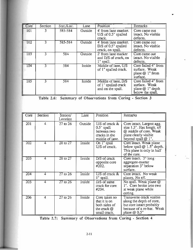
1 Table 2.6: Summary of Observations from Coring

Outside

Remarks 11

crack. 4' from lane marker. D/S of 0.5" spalled

584

3

105

Core came out intact. No visible defects.

intact, No visible

intact. No visible Outside

584

3

surface. Weak plane @ 1" from surface.

surface. Weak

crack, on spdl. 2' from lane marker

plane @ 1" depth

Inside

584

- Section 3

1" spall. Middle of lane, U/S

Inside

Table 2.7: Summary of Observations from Coring - Section 4

Middle of lane, D/S of 1 " spalled crack

Remarks

Core intact. Largest agg. size 1.5". Has longit. r/f @ middle of core. Weak plane clearly visible beyond spall @ 1". Core intact. Weak plane below spall @ 1.5" depth. This plane is only in half of the core. Core intact. 3': long aggregate-mortar separation 3" below surface. Core intact. No weak planes. No rlf. No spall. Weak plane @ 1 ". Core broke into two at weak plane while coring.

206 4 27 to 26 Inside Core taken so Transverse crack visible that it is on along the depth of core, both sides of but core intact probably the crack @ because of a re-bar. Weak small crack. plane @ 0.5"

Core

201

202

203

204

205

Station/ Location 27 to 26

28 to 27

28 to 27

27 to 26

27 to 26

Section

4

4

4

4

4

Lane

Outside

Inside

Inside

Inside

Inside

Position

U/S of crack & 0.5" spall between two cracks in the middle of lane. On 1" s p a U/S of crack.

D/S of crack opposite core #202.

U/S of crack & 1" spall. D/S of same crack for core #204.

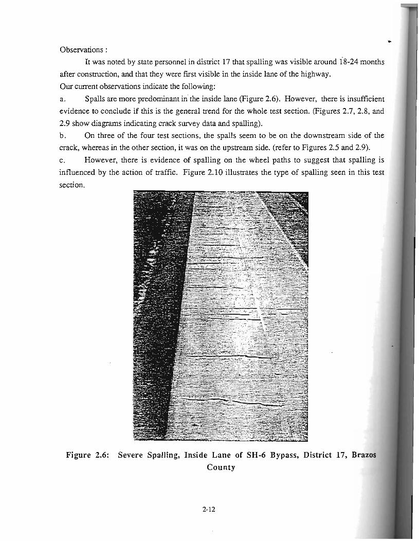
Observations : It was noted by state personnel in district 17 that spalling was visible around 18-24 months

after construction, and that they were fxst visible in the inside lane of the highway.

Our current observations indicate the following:

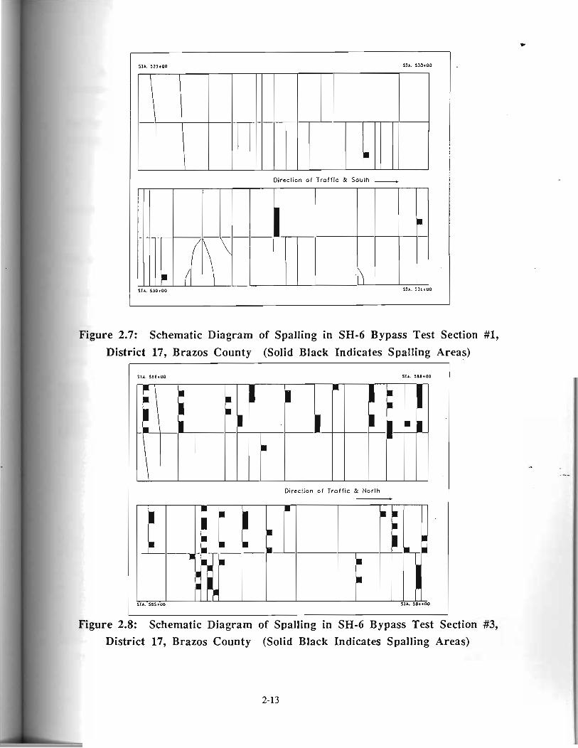
a. Spalls are more predominant in' the inside lane (Figure 2.6). However, there is insufficient

evidence to conclude if this is the general trend for the whole test section. (Figures 2.7,2.8, and

2.9 show diagrams indicating crack survey data and spalling).

b. On three of the four test sections, the spalls seem to be on the downstream side of the

crack, whereas in the other section, it was on the upstream side. (refer to Figures 2.5 and 2.9).

c. However, there is evidence of spalling on the wheel paths to suggest that spalling is

influenced by the action of traffic. Figure 2.10 illustrates the type of spalling seen in this test

section.

Figure 2.6: Severe Spalling, Inside Lane of SH-6 Bypass, District 17, Brazos

County

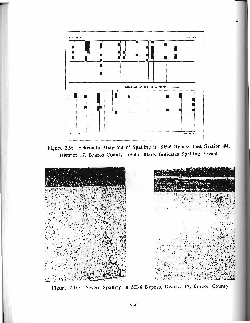
I i Figure 2.9: Schematic Diagram of Spalling in SH-6 Bypass Test Section #4, I

District 17, Brazos County (Solid Black Indicates Spalling Areas) i

Figure 2.10: Severe Spalling in SH-6 Bypass, District 17, Brazos County

2-14

A general observation made from these cores was the presence of delaminations in the

pavement very close to the surface at a depth of approximately 0.5 to 1 inches from the surface. Some delaminations were significant enough to be detected by the sound emanating from a

steel bar dropped on the pavement.

This approximate method of detection of delaminations indicated that:

a. Delaminations are randomly distributed across the lane.

b. Delaminations are present on both lanes.

c. Delaminations are always adjacent to a crack, a joint, or an edge. However, the most

common location was adjacent to transverse cracks.

2.2.2 Beltway 8 Frontage Road in Harris County

This section of the highway was completed in 1987.

Location :

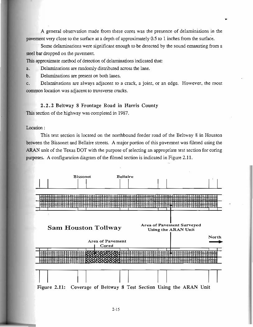
This test section is located on the northbound feeder road of the Beltway 8 in Houston

between the Bissonet and Bellaire streets. A major portion of this pavement was filmed using the

ARAN unit of the Texas DOT with the purpose of selecting an appropriate test section for coring

purposes. A configuration diagram of the filmed section is indicated in Figure 2.11.

Sam Houston Tollway

Bissonet Bellaire

I Area of Pavement Surveyed

Using the ARAN Unit

I

Area of Pavement

I

North - I Cored I

I

Figure 2.11: Coverage of Beltway 8 Test Section Using the ARAN Unit

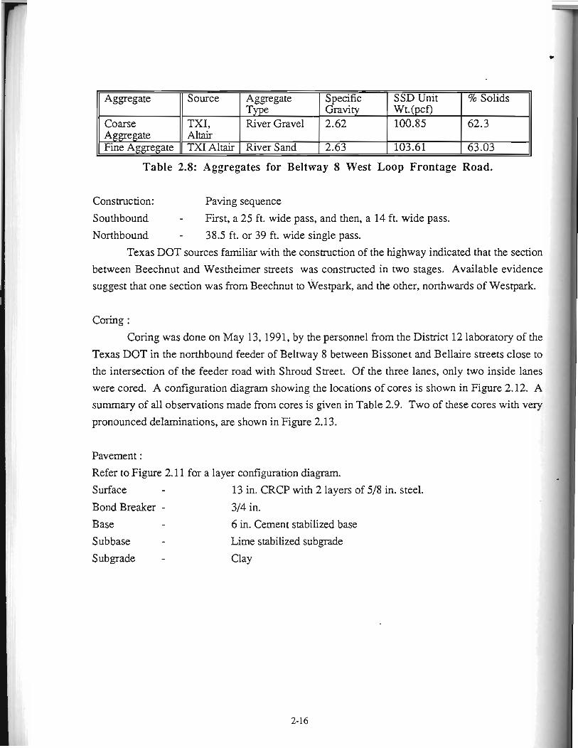
Aggregate Source Aggregate Specific SSD Unit % Solids Type Gravity Wt. (pcf)

Coarse TXI, River Gravel 2.62 100.85 62.3 Aggregate Altair Fine Aggregate TXI Altair River Sand 2.63 103.61 63.03

Table 2.8: Aggregates for Beltway 8 West Loop Frontage Road.

Construction: Paving sequence

Southbound - Fist, a 25 ft. wide pass, and then, a 14 ft. wide pass. I

Northbound - 38.5 ft. or 39 ft. wide single pass. I I

Texas DOT sources familiar with the construction of the highway indicated that the section I

between Beechnut and Westheimer streets was constructed in two stages. Available evidence suggest that one section was from Beechnut to Westpark, and the other, northwards of Westpark. t

Coring :

Coring was done on May 13, 1991, by the personnel from the District 12 laboratory of the

Texas DOT in the northbound feeder of Beltway 8 between Bissonet and Bellaire streets close to

the intersection of the feeder road with Shroud Street. Of the three lanes, only two inside lanes

were cored. A configuration diagram showing the locations of cores is shown in Figure 2.12. A

summary of all observations made from cores is given in Table 2.9. Two of these cores with very

pronounced delaminations, are shown in Figure 2.13.

Pavement :

Refer to Figure 2.11 for a layer configuration diagram.

Surface - 13 in. CRCP with 2 layers of 5/8 in. steel.

Bond Breaker - 314 in.

Base - 6 in. Cement stabilized base

Subbase - Lime stabilized subgrade

Subgrade - Clay

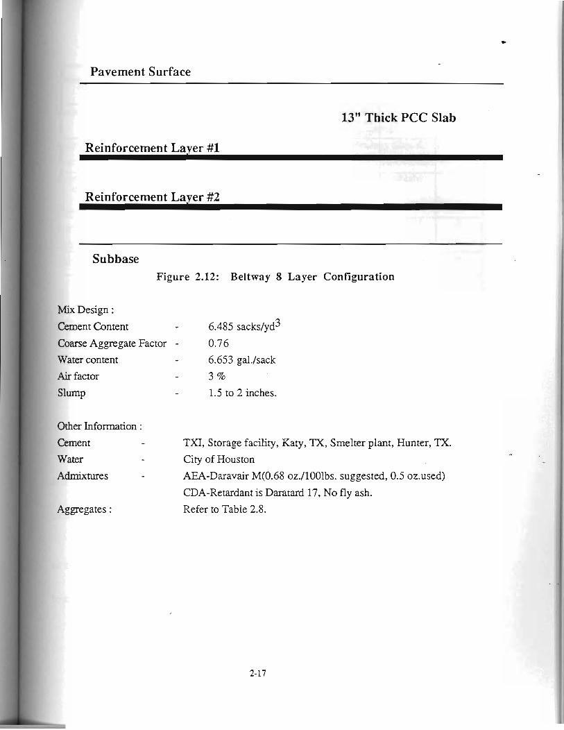
Pavement Surface

13" Thick PCC Slab

Reinforcement Lager #1

Subbase Figure 2.12: Beltway 8 Layer Configuration

Mix Design :

Cement Content - 6.485 sackdYd3

Coarse Aggregate Factor - 0.76

Water content - 6.653 gal./sack - 3 % Air factor

Slump - 1.5 to 2 inches.

Other Information : Cement - TXI, Storage facility, Katy, TX, Smelter plant, Hunter, TX.

Water - City of Houston

Admixtures - AEA-Daravair M(0.68 oz./1001bs. suggested, 0.5 oz-used)

CDA-Retardant is Daratard 17, No fly ash.

Aggregates : Refer to Table 2.8.

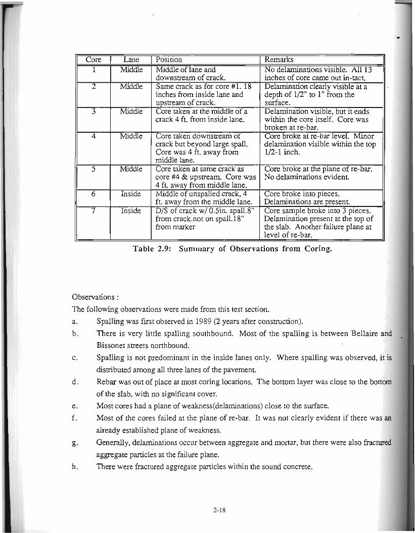
Core Lane Position Remarks 1 Middle Middle of lane and No delaminations visible. All 13

downstream of crack. inches of core came out in-tact. 2 Middle Same crack as for core #1. 18 Delamination clearly visible at a

inches from inside lane and depth of 1/2" to 1" from the upstream of crack surface.

3 Middle Core taken at the middle of a Delamination visible, but it ends crack 4 ft. from inside lane. within the core itself. Core was

broken at re-bar. 4 Middle Core taken downstream of Core broke at re-bar level. Minor

crack but beyond large spall. delamination visible within the top Core was 4 ft. away from 1/2-1 inch. middle lane.

5 Middle Core taken at same crack as Core broke at the plane of re-bar. core #4 & upstream. Core was No delaminations evident. 4 ft. away from middle lane.

6 Inside Middle of unspalled crack, 4 Core broke into pieces.. ft. away from the middle lane. Delaminations are present

7 Inside D/S of crack w/ 0.511. spall.8" Core sample broke into 3 pieces. from crack-not on spall. 18" Delamination present at the top of from marker the slab. Another failure plane at

level of re-bar.

Table 2.9: Summary of Observations from Coring.

Observations :

The following observations were made from this test section.

a. Spalling was first observed in 1989 (2 years after construction).

b. There is very little spalling southbound. Most of the spalling is between Bellaire and

Bissonet streets northbound.

c. Spalling is not predominant in the inside lanes only. Where spalling was observed, it is

distributed among all three lanes of the pavement.

d. Rebar was out of place at most coring locations. The bottom layer was close to the bottom

of the slab, with no significant cover.

e. Most cores had a plane of weakness(delaminations) close to the surface.

f . Most of the cores failed at the plane of re-bar. It was not clearly evident if there was an

already established plane of weakness.

g. Generally, delaminations occur between aggregate and mortar, but there were also fractured 1 aggregate particles at the failure plane.

h. There were fractured aggregate particles within the sound concrete.

2.2.3 Interstate 45 in Leon County

This section of the highway was completed in 1972.

Location :

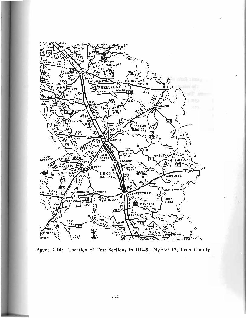
Of the original CRC pavement of the Interstate 45 highway, except for a 20 mile stretch

extending from State highway 7 at Centerville up to the Freestone county line, all the rest of has

been overlaid with 4 - 7 inches of asphalt concrete. This whole non-overlaid section was

considered as one test section (Figure 2.14).

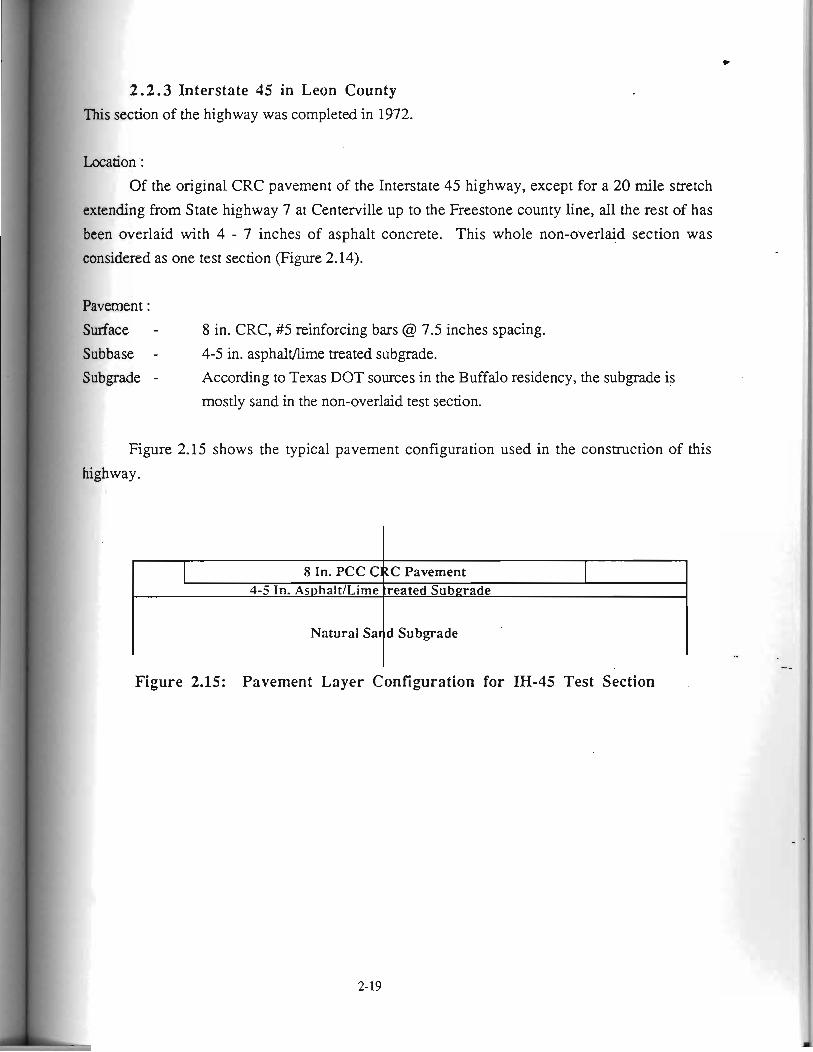
Pavement :

Surface - 8 in. CRC, #5 reinforcing bars @ 7.5 inches spacing.

Subbase - 4-5 in. asphalflime treated subgrade.

Subgrade - According to Texas DOT sources in the Buffalo residency, the subgrade is

mostly sand in the non-overlaid test section.

Figure 2.15 shows the typical pavement configuration used in the construction of this

highway.

I 8 In. PCC CXC Pavement I 4-5 In. As~haltILirne :reated Subgrade

Natural Sar d Subgrade

Figure 2.15: Pavement Layer Configuration for IH-45 Test Section .

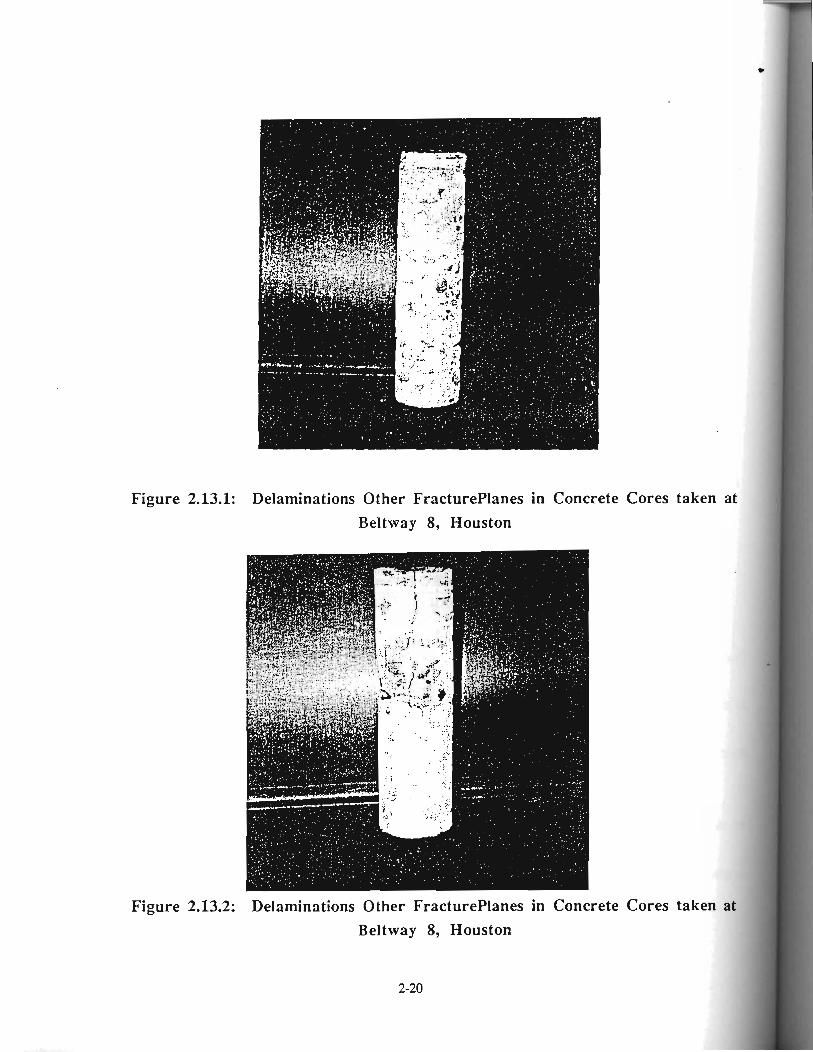
Figure 2.13.1: Delaminations Other FracturePlanes in Concrete Cores taken at

Beltway 8, Houston I

I Figure 2.13.2: Delaminations Other Fractureplanes in Concrete Cores taken at

Beltway 8, Houston

2-20

Mix design :

Cement content - 4.5 sacks/yd3

Water content - 6.2 gal./sack

Coarse Aggregate Factor - 0.80

Air factor - 4 percent

Slump - 1.5 to 2 inches

Aggregates : Refer to Table 10 below.

The records indicate that 3 combinations of the coarse aggregate types were used in the

concrete. They are:

1. 65% East Texas Stone Crushed Limestone and 35% Holsey Bros. Gravel.

2. 65% Gifford Hill Gravel and 35% East Texas Stone Crushed Limestone.

3. 100% Crushed Sandstone East Texas Stone Co.

Other Information:

Cement - Atlas Cement Co., Waco.

Water - Local Lake.

Admixtures - AEA Scotch (Dosage: 35 oz. for 8 yd3 of concrete).

Category Source Aggregate Spec. SSD Unit % Trpe Gravity Wt.(pcf) Solids

Coarse Blue Mm. Pit, Crushed 2.64 81.91 55.7 Aggregate 1 East Calcareous

Texas Stone Co. Sandstone Coarse Holsey Bros., Siliceous 2.61 103.91 63.7 Aggregate 2 Austonio. Gravel

Coarse Gifford Hill,- Crushed 2.65 97.55 58.9 Aggregate 3 Wardlaw Pit. Limestone1

Siliceous Gravel

Fine Holsey Bros., Siliceous- 2.66 94.76 57.0 AgSFgate Aus tonio. Limestone

Sand L

Table 2.10: Details on Aggregates for IH-45 in Buffalo, TX.

Construction:

Both highway lanes in one direction has been laid in one paving operation.

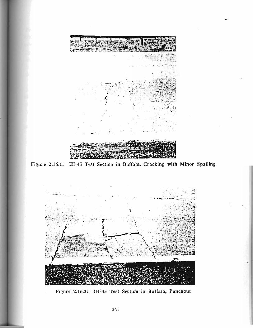
Observations: Spalling is almost non-existent in this test section of 80 lane miles. The primary mode of

failure is punchouts. A quick count of the number of punchout failures indicated the following

data.

Number of punchout failures northbound = 5

Number of punchout failures southbound = 16

A typical punchout and transverse cracking in this test section is shown in Figure 2.16.

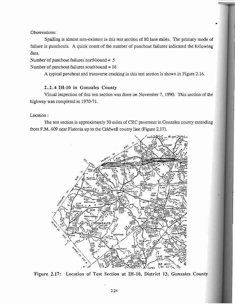
I 2 .2 .4 IH-10 in Gonzales County I Visual inspection of this test section was done on November 7, 1990. This section of the

highway was completed in 1970-7 1.

Location :

The test section is approximately 30 miles of CRC pavement in Gonzales county extending

from F.M. 609 near Flatonia up to the Caldwell county line (Figure 2.17).

I

Figure 2.17: Location of Test Section at IH-10, District 13, Gonzales County

Pavement :

I The typical pavement configuration used in the construction of this highway is indicated below.

Section East of SH-304

Surface - 8 in. thick CRC, with one reinforcement mat.

Subbase - 4 in. black base and lime stabilized subgrade.

Subgrade - Clay.

Section West of SH-304

Surface - 8 in. thick CRC, with one reinforcement mat.

Subbase - 8-10 in. cement-soil mixture.

Subgrade - Sand.

Mix design: Not available.

Aggregates:

No infoxmation is available, but our observations indicate that it is a crushed stone.

Construction:

The two segments of the highway on either side of SH-304 were constructed as separate

projects (Figure 2.17). In both segments all 24 ft. of pavement was laid using the slipfom

method. Shoulder is asphalt concrete.

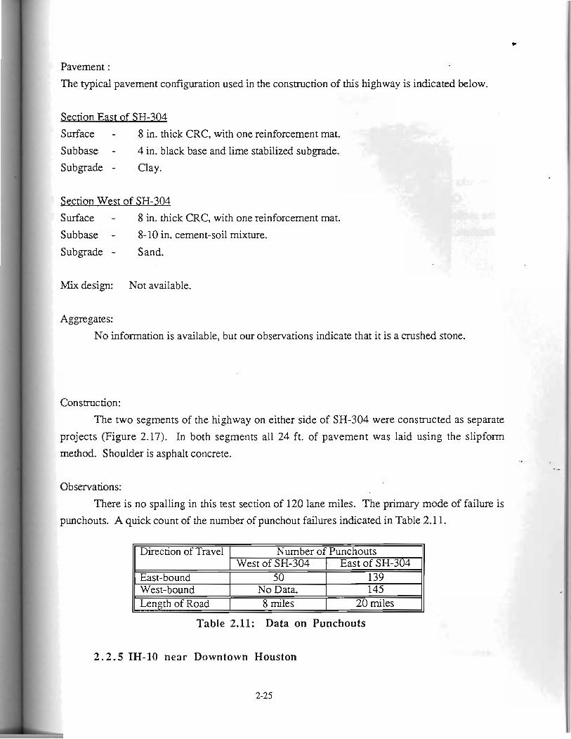
Observations:

There is no spalling in this test section of 120 lane miles. The primary mode of failure is

punchouts. A quick count of the number of punchout failures indicated in Table 2.11.

Direction of Travel West of SH-304

West-bound No Data. 8 miles

Table 2.11: Data on Punchouts

2.2.5 IH-10 near Downtown Houston

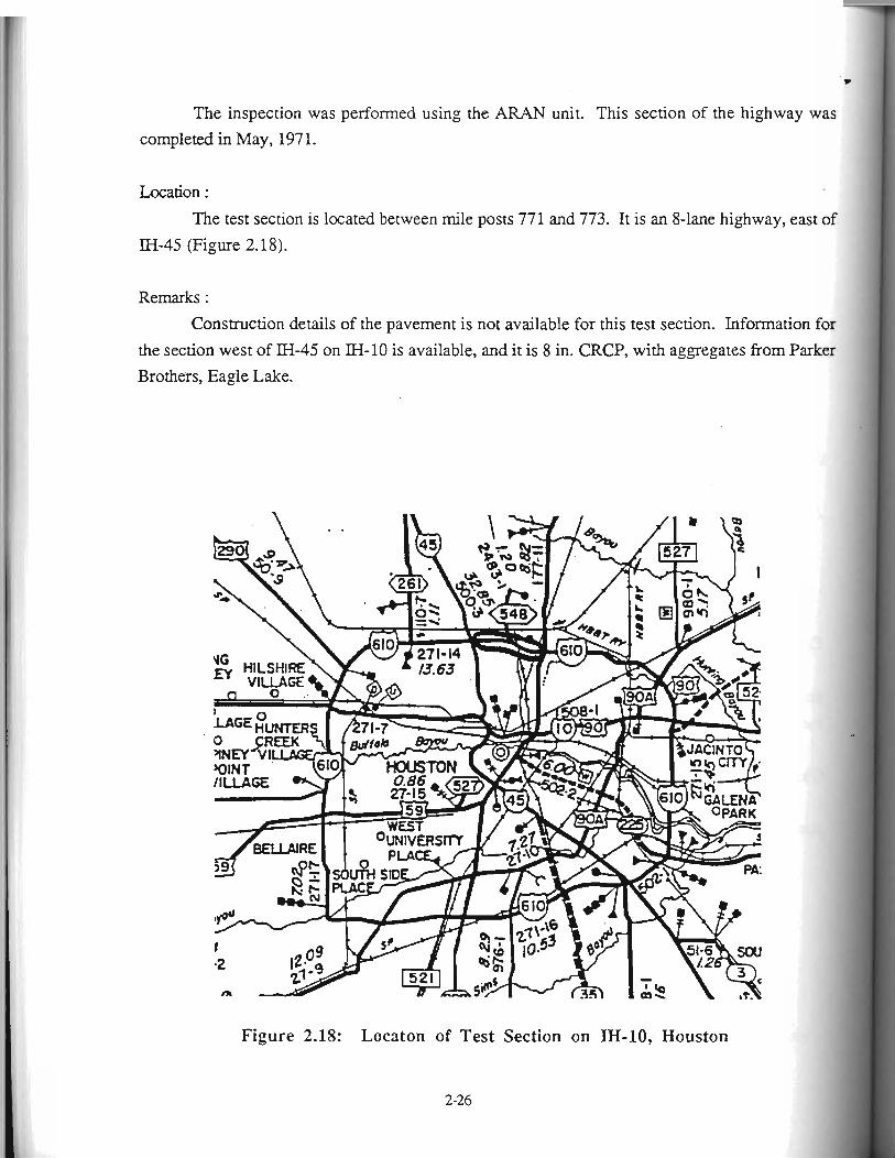
The inspection was performed using the ARAN unit. This section of the highway was

completed in May, 197 1.

Location :

The test section is located between mile posts 771 and 773. It is an 8-lane highway, east of

IH-45 (Figure 2.18).

Remarks :

Construction details of the pavement is not available for this test section. Information for

the section west of IH-45 on IH-10 is available, and it is 8 in. CRCP, with aggregates from Parker

Brothers, Eagle Lake.

Figure 2.18: Locaton of Test Section on IH-10, Houston

2-26

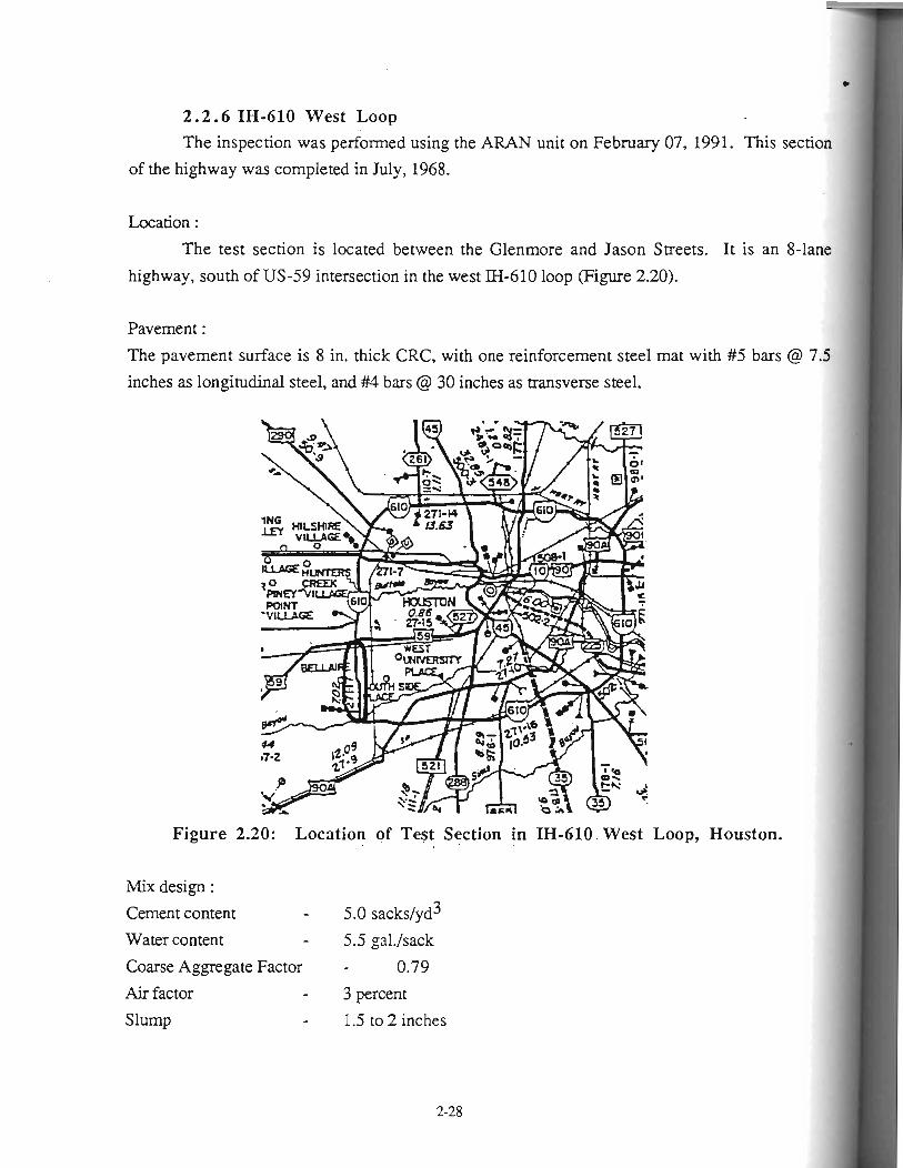
2.2.6 IH-610 West Loop

The inspection was performed using the ARAN unit on February 07, 1991. This section

of the highway was completed in July, 1968.

Location :

The test section is located between the Glenmore and Jason Streets. It is an 8-lane

highway, south of US-59 intersection in the west IH-610 loop (Figure 2.20).

Pavement :

The pavement surface is 8 in. thick CRC, with one reinforcement steel mat with #5 bars @ 7.5

inches as longitudinal steel, and #4 bars @ 30 inches as transverse steel.

Figure 2.20: Location of Test Section in IH-610. West Loop, Houston.

Mix design :

Cement content - 5.0 sackslyd3

Water content - 5.5 galhack

Coarse Aggregate Factor - 0.79

Air factor - 3 percent

Slump - 1.5 to 2 inches

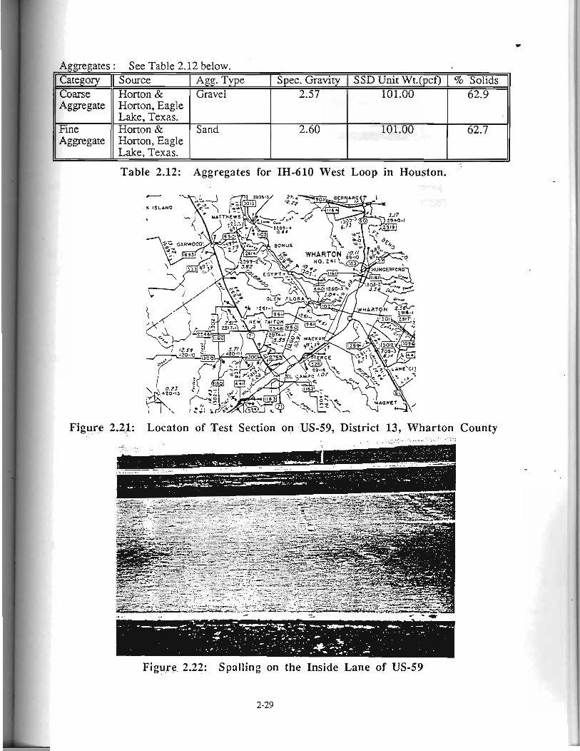
Aggregates : See Table 2.12 below. Category Source Ags. Type Spec. Gravity SSD Unit Wt.(pcf) % Solids Coarse Horton & Gravel 2.57 101.00 62.9 Aggregate Horton, Eagle

Lake, Texas. Fine Horton & Sand 2.60 101.00 62.7 Aggregate Horton, Eagle

Lake, Texas.

Table 2.12: Aggregates for IH-610 West Loop in Houston.

Figure , .

Figure 2.22: Spalling on the Inside Lane of US-59

2-29

County

Other Information :

Cement - Type I Cement from Trinity, Houston.

Admixture - Solar.025,4 oz. (AEA)

Construction: No information is available.

Observations:

The pavement is extensively cracked, and spalled as well. The spalls are not limited to the

inside lanes only.

7. US-59 in Wharton County

The test section was in service for around 20 years. It is located between Wharton and El Campo in Texas DOT district 13 (Figure 2.21). No detailed investigations were done in this section. However, the remaining non-overlaid sections indicated the following.

1 . River gravel was used as the coarse ag,gregate in concrete.

2. There was extensive spalling in both directions of the highway.

3. Most of the spalling was in the inside lane (Figure 2.22).

4. There was some indication of spalling along the wheelpaths. However, there were exceptions to this too.

5. Texas DOT sources in Yoakum district office have noticed that spalling occurred 5 to 7 years after placement of concrete. They also said that there is very little spalling in the

longitudinal joints or cracks.

2 .3 SUMMARY OF FIELD INVESTIGATIONS

The field investigation phase indicated some very significant observations.

They are :

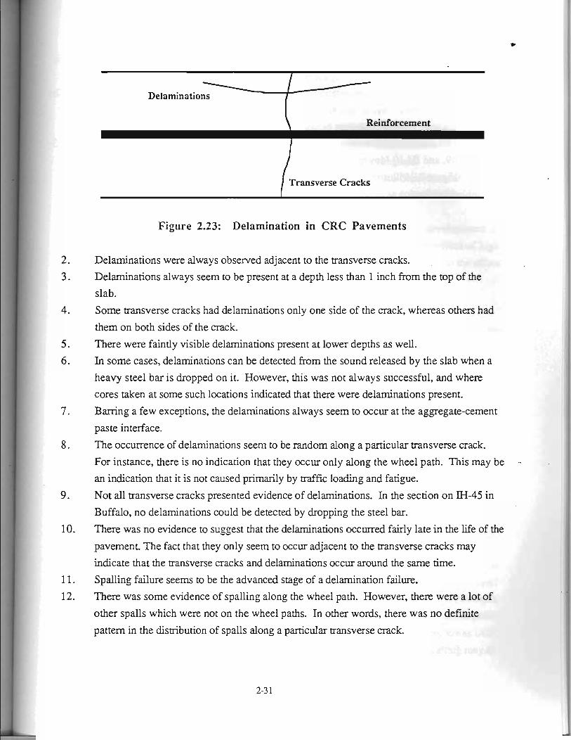
1. Coring of the CRC pavements showed that there are horizontal delaminations in the slab

very close to its surface, generally extending up to a distance of a few inches from the crack

(Figure 2.23).

Delaminations s \ Reinforcement

Transverse Cracks

Figure 2.23: Delamination in CRC Pavements

1 2. Delaminations were always observed adjacent to the transverse cracks. .

3. Delaminations always seem to be present at a depth less than 1 inch from the top of the

slab.

4. Some transverse cracks had delaminations only one side of the crack, whereas others had

them on both sides of the crack.

5 . There were faintly visible delaminations present at lower depths as well.

6 . In some cases, delaminations can be detected from the sound released by the slab when a

heavy steel bar is dropped on it. However, this was not always successful, and where

cores taken at some such locations indicated that there were delaminations present.

7 . Baning a few exceptions, the delarninations always seem to occur at the aggregate-cement

paste interface.

8. The occurrence of delaminations seem to be random along a particular transverse crack.

For instance, there is no indication that they occur only along the wheel path. This may be

an indication that it is not caused primarily by traffic loading and fatigue.

9. Not all transverse cracks presented evidence of delaminations. In the section on IH-45 in

Buffalo, no delaminations could be detected by dropping the steel bar.

10. There was no evidence to suggest that the delaminations occurred fairly late in the life of the

pavement The fact that they only seem to occur adjacent to the transverse cracks may

indicate that the transverse cracks and delaminations occur around the same time.

1 1. Spalling failure seems to be the advanced stage of a delamination failure.

12. There was some evidence of spalling along the wheel path. However, there were a lot of

other spalls which were not on the wheel paths. In other words, there was no definite

pattern in the dismbution of spalls along a particular transverse crack.

*

13. The orientation of the spa11 with reference to the transverse crack (i.e. on which side of the

transverse crack the spalling takes place), seem to be a factor that needs to be considered.

There was a definite orientation of spalls in the test sections of SH-6 and US-59, where the

spalls were always on one side of the transverse crack. However, some spalls in the .

Beltway 8 test section were on either side of the transverse crack 14. More spalls seem to occur in the inside lane than the outside lane, particularly in SH-6, US-

59, and IH-10 (downtown Houston) test sections.

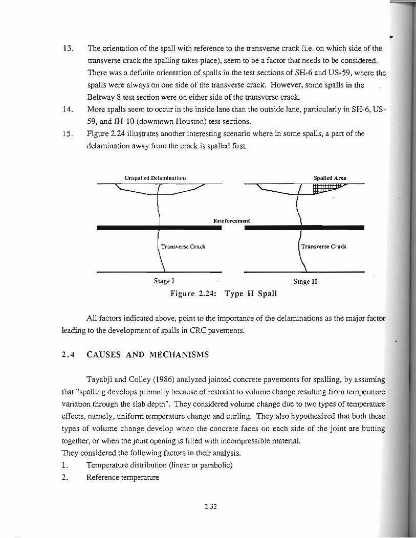
15. Figure 2.24 illustrates another interesting scenario where in some spalls, a part of the

delamination away from the crack is spalled first.

Unspalled Delaminations Spalled Area

Reinforcement

Transverse Crack Transverse Crack

Stage I Stage I1

Figure 2.24: Type I1 Spall

All factors indicated above, point to the importance of the delarninations as the major factor

leading to the development of spalls in CRC pavements.

2.4 CAUSES AND MECHANISMS

Tayabji and Colley (1986) analyzed jointed concrete pavements for spalling, by assuming

that "spalling develops primarily because of restraint to volume change resulting from temperature

variation through the slab depth". They considered volume change due to two types of temperature

effects, namely, uniform temperature change and curling. They also hypothesized that both these

types of volume change develop when the concrete faces on each side of the joint are butting

together, or when the joint opening is filled with incompressible material.

They considered the following factors in their analysis.

1. Temperature distribution (linear or parabolic)

2. Reference temperature

w

3. Joint restraint condition (free or restrained)

The analysis was made using a finite element computer program for a slab 10 in. thick and

20 feet long. The subgrade was modelled using truss elements and a subgrade modulus of 100 pci

was used.

The results of their analysis indicate that increased restraint increases the compressive

stresses at the top of the slab, and also that a differential temperature distribution results in lower

tensile stresses at the bottom of the slab as a result of restraint from the subgrade.

Stress analysis performed by Zollinger and Barenberg (1988) also demonstrated that the

position of the longitudinal stress, condition on the subgrade support, and the crack width can

significantly affect the development of spalling.

These results are important indicators of the factors involved in the development of

spalling. However, one must also consider the state of the concrete prior to the effect of high

temperature induced compressive stresses at the top fibers of the slab. This leads us to the effect .

shrinkage and creep of early age concrete has on the behavior and of concrete.

2.4.1 Role of Delaminations in Spalling From the summary of field -investigations, it is quite evident that spalling is preceded by

delamination of the pavement slab adjacent to the transverse cracks and joints. This may also

suggest that, either the delaminations occur at the same tome as the transverse cracks, or, de-

bonding of the aggregate-cement paste very close to the surface during transverse cracking is later

aggravated into a continuous flaw. This may take place due to several factors such as load due to

traffic, temperature change, effects of expansive soils, and further hydration.

2.4.2 Orientation of spall Investigation of spalling, particularly in the SH-6 and US-59 test sections, indicate that .-

- spalling may take place only on one side of the transverse crack. However, coring of the SH-6 test

section indicated that at some of these locations, there were delarninations on both sides of the

crack. This may suggest that due to several factors, there can be a difference in the size of the

delamination on either side of the crack, and during subsequent loading would result in spalling

only on one side of the crack. An interesting feature of the SH-6 test section was that more than 75 percent of the

pavement is spalled on the downstream side of the transverse crack (in the direction of traffic), and

the rest is spalled on the upstream side (Figure 2.5). Further investigations indicated that this

reversal of spall orientation occurred near SH-21 intersection where the concrete mixing plant has

been located during construction. Information obtained from sources in District 17 of Texas DOT

who were involved in the construction of the project indicate that this direction of spalling may be

*

related to the direction of paving in some way. However, no concrete data on paving sequence was available from the district, and therefore, no conclusive judgement could be made on this

issue.

2.4.3 More spalling in the inside lane Of the sections investigated, the sections on SH-6, US-59 and M-10 in Houston showed

evidence of significantly more spalling in the inside lane(s) of the highway. Of these three test sections, from what we observed, at least SH-6 and US-59 sections do not seem to cany much

traffic in the inside lane. This probably leads us to believe that either traffic does not have much

influence on the development of the spall, or that there are factors other than traffic which enable

spalls to develop from delaminations. However, some of the spalling we have seen on wheelpaths

may indicate that traffic couId indeed be a factor affecting the development of spalls. The

difference in spalling between inside and outside lanes made us look for differences between them.

I In SH-6 and US-59, both lanes have been laid together, and they both have the same design

parameters. The only difference seems to be in the amount of traffic each lane carries.

From the studies made by Tayabji and Colley, they pointed out the important role played by

restraint at transverse cracks in generating larger stresses which may lead to spalling. This

combined with the assertion by Zollinger and Barenberg (1988) whose stress analysis

demonstrated that the crack width can significantly affect the development of spalling makes us

speculate that there may be a high degree of restraint in the inside lane which restricts it from

expanding during high temperatures. Unfortunately, at this point, we do not have any data on the

timing of spalling in terms of seasons of weather. This may shed some light on this observation.

A theory developed by Thouless (1985), for spalling of flat plates by thermal shock seems

appropriate in this regard. He considered that the spalling originates from a smaller flaw within the

medium. He developed his theory considering the buckling of the plates as a result of higher -

compressive stresses. He devised a critical flaw size which would propagate as a result of

buckling, and made it variable with time, measured since the occurrence of thermal shock.

2.4.4 Direction of paving

As it was mentioned under observations of SH-6 test sections, we have reason to believe

that the direction of paving may have some influence on the orientation of the spalls.

Unfortunately, no documented evidence is available on the construction of the SH-6, and

therefore, no judgement could be made. But we can think of a scenario where formation of the'

delaminations being affected by the degree of restraint on shrinkage, vis-a-vis the direction of

paving. Once the delaminations are formed, the factors which affect the development of the spall,

such as traffic, temperature effects, and sub,pde effects may come into play.

2-34 I

2.4.5 Aggregate effects Of the seven pavement test sections investigated, gravel was the coarse aggregate for five

of the sections, one had crushed limestone, and the other had a blend of crushed calcareous

sandstone and gravel. The two sections which used crushed stone aggregates did not show any

significant spalling. They only displayed cracking and punchout distresses. At this point, we do

not have sufficient evidence to suggest that it is the type of coarse aggregate that is causing a11 this

spalling in CRC pavements. There may be a number of other factors related to the construction

such as the mix design and the type of curing mechanism used, which may also have a significant influence on the development of delaminations, and hence the spalls. However, we cannot

discount the evidence we have suggesting that a number of concrete pavements with gravel

aggregates have spalled, while keeping in mind that not all concrete pavements with gravel

aggregates have spalled.

2.4.6 Subgrade effects The evidence from the IH-45 test section suggested to us that a clay subgrade which may

be expansive, can have some effect on the spalling of concrete pavements. Stresses acting on the

pavement as a result of shrinkage and swelling of expansive clays may add to the list of other

factors such as temperature effects and traffic load which contribute to the stressing of pavements.

The test section on IH-45 in Gonzales county had both a clay and a sand subgrade, but neither section showed any spalling.

2.4 .7 Construction effects

Concrete mix design properties and the method of curing are two aspects of construction

that has a profound impact on the performance of concrete pavements. An effective method of .-

curing should eliminate most of the shrinkage stresses from early age concrete. The mix design

can be orchestrated in such a way to reduce the shrinkage stresses, but at the same time, to increase

the development of strength, pamcularly at the interface between aggregate and the cement paste.

The bond strength and the rate of increase of bond strength could be increased by having a

better cement and/or a high water-cement ratio. This in turn may increase the shrinkage strain and

the generation of heat during the hydration process. On the other hand, increase of water content

for ease of placement can increase shrinkage strains considerably. This calls for more effective

curing methods.

Therefore, it is evident that the factors involved in the mix design often interact with each

other which makes it imperative to have a very good understanding of the bond strength between

* aggregate and the cement paste. This shows the importance of studying the development of delamination and spalling of CRC pavements in a controlled setting.

I I 2.5 REFERENCES

2.1. Tayabji, S.D. and Colley, B.E., "Improved Rigid Pavement Joints", Research Report

FHWA/RD-86/040, Construction Technology laboratories, A Division of Portland Cement

Association, Skokie, Illinois, February 1986.

2.2. Thouless, M.D., "Spalling of Flat Plates by Thermal Shock", Journal of the American

Ceramic Society, 68(4), C-111-C-112,1985.

2.3. Zollinger, D.G., and Barenberg, E.J., "Continuously Reinforced Pavements : Punchouts

and other Distresses and Implications for Design", Research Report No. FHWA/IL/UI

227, Illinois Department of Transportation, Department of Civil Engineering, Engineering

Experiment Station, University of Illinois, Urbana, March 1990.

2.4. Epps, J.A., Meyer, A.H., Larrimore, I.E., and Jones, H.L., "Roadway Maintenance

Evaluation User's Manual", Research Report 151-2, Texas Highway Department, Texas

Transportation Institute, College Station, Texas, September, 1974.

2.5. Rater's Manual, Texas State Department of Highways and Public Transportation, 1985.

2.6. Personal communication with Professor B. Galloway, Professor Emeritus, Texas A & M

University, 1990.

F-

CHAPTER 3

BASIC FAILURE MODES LEADING TO PUNCHOUT DISTRESS IN CRC PAVEMENT

I 3 .1 BASIC FAILURE MODES I I I

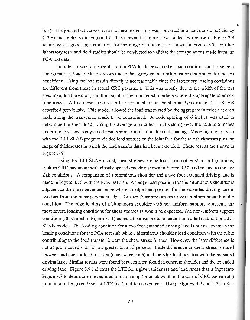
Four failure modes relating to punchout distress based on the previous field studies can be

considered as fundamental thickness design mechanisms for CRC pavements. The analysis of the

failure modes is based apriori on uniform support conditions. This requires the use of a non or

low erodible subbase. The failure modes are illustrated in Figure 3.1 in typical developmental

sequence. Mode I failure is fracturing due to reinforcing bar pullout from the surrounding

concrete. Fracturing of this nature has been noted in concrete pullout tests (3.1,3.2) and develops .

in the concrete at a steel stress range of 14 to 18 ksi. Field measurements of steel strains at the

crackface indicate that this range of stress is frequently exceeded in the colder months of the year.

Cyclic bond stresses in the concrete induced from environmental factors can result in a crack

growth process, noted in the field study, around the reinforcing bar effectively destroying the load

transfer capability of the bar as a void develops. Additionally, a loss of bond stiffness (3.3) and

pavement bending stiffness occurs. Bearing failure or rebar looseness can also lead to a void around the reinforcement and can have a demmental effect upon the pavement performance similar

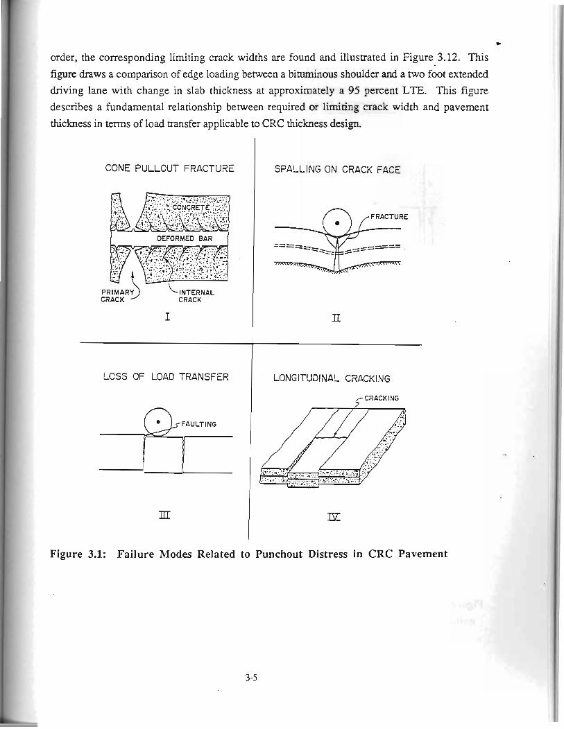
to what the pullout fracture does. Pullout failure may be difficult to avoid since the threshold stress

is frequently exceeded as illustrated in Figure 3.2 for a steel percentage of 0.7 in terms of crack

spacing and temperature drop. Increasing the steel percentage to 0.9 reduces the stresses

approximately 1 percent. Therefore, the load transfer contribution of the reinforcing bar should be

ignored.

Mode 11, spalling of the transverse crack, is a function of the pavement stiffness. Due to

the above assumption with regard to the development of rebar voids, the pavement stiffness is

affected accordingly inasmuch as it is significantly reduced. A certain amount of support loss can

be allowed since results from the field study indicate that good performing CRC pavements have

experienced some loss of edge support. As suggested in one study, a reduction in pavement

stiffness at the cracks may also develop due gradual joint deterioration and declining load transfer

efficiency (3.4). These conditions are adequate justification to determine spa11 related stresses

based on a reduced pavement stiffness. The pavement stiffness cycles between high and low,

mostly as a function of the temperature and the concomitant opening and closing of the cracks.

The reduced stiffness behavior, which occurs on a daily basis, can be assumed to predominate

during the winter season. Reduced pavement stiffness is not only a function of the crack width

* (3.5) but also of the position of the reinforcing steel (3.6) among other factors. Therefore, spall

related stresses can be determined as a function of the pavement stiffness, design crack width, steel

percentage, and the position of the reinforcement in the slab. The narrower the transverse cracks . .

the stiffer the overall pavement system, which in tum lowers the spall related stresses. This mode

of failure is a visual sign of progressive punchout development.

Failure mode 111, shown in Figure 3.1, is a loss of load transfer along transverse cracks.

Since the bar is assumed to provide no load transfer, the load transfer of the crack is solely a function of the crack width. Given a constant crack width, the load transfer will decrease under

repetitive loading. The resulting load tnnsfer efficiency is based on test results by PCA (3.7) for

one million load applications which an intrepreted as a million coverages.

The final mode of failure, mode IV, is related to bending stresses in the transverse

direction. These stresses typically are not significant in CRC pavement so long as there is a high load transfer across the cracks (prior to spalling) or the crack spacing is greater than 4 feet.

Transverse bending stresses should be considered in most instances since the crack spacing

distribution in CRC pavement typically ranges below 4 feet. The load transfer was noted to

decrease significantly with spalling (type 2) in CRC pavements with thicknesses between 8 to 10

inches. The transverse bending stresses should be increased in response to the change in load

transfer.

As suggested in the description of mode I failure, a reduction in pavement stiffness may result either from pullout failure or from bearing failure around the steel, both of which have been

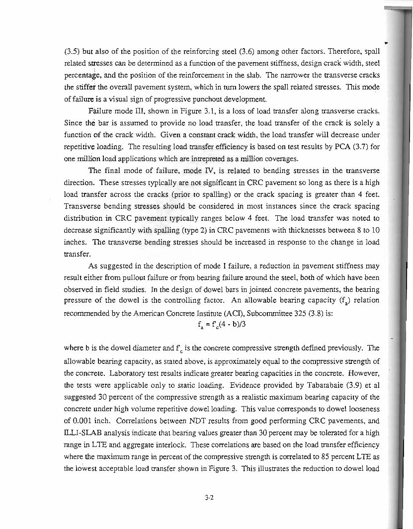
observed in field studies. In the design of dowel bars in jointed concrete pavements, the bearing pressure of the dowel is the controlling factor. An allowable bearing capacity (fa) relation

recommended by the American Concrete Institute (ACI), Subcommittee 325 (3.8) is: fa = f =(4 - b)/3

where b is the dowel diameter and f, is the concrete compressive strength defined previously. The

allowable bearing capacity, as stated above, is approximately equal to the compressive strength of

the concrete. Laboratory test results indicate greater bearing capacities in the concrete. However,

the tests were applicable only to static loading. Evidence provided by Tabatabaie (3.9) et al

suggested 30 percent of the compressive strength as a realistic maximum bearing capacity of the

concrete under high volume repetitive dowel loading. This value corresponds to dowel looseness

of 0.001 inch. Correlations between NDT results from good performing CRC pavements, and

ELI-SLAB analysis indicate that bearing values greater than 30 percent may be tolerated for a high

range in LTE and aggregate interlock. These correlations are based on the load transfer efficiency

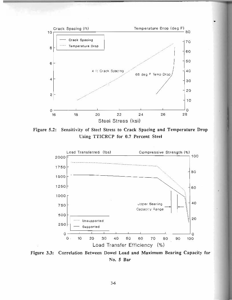
where the maximum range in percent of the compressive strength is correlated to 85 percent LTE as

the lowest acceptable load transfer shown in Figure 3. This illustrates the reduction to dowel load

*

with an increase in load transfer due to lower crack width (improved aggregate interlock) for

uniform and non-uniform support conditions. Based on a concrete compressive strength of 6000

psi, the percent reduction of the compressive strength (which is the allowable bearing capacity of the concrete), using the ACI equation and Friberg's dowel deflection analysis (3.10), is shown

correlated to the dowel load for a No. 5 reinforcing bar. Since the load transfer efficiency of

adequately performing CRC pavement usually ranges between 85 and 95 percent, Figure 3.3

suggests a range for the upper bearing capacity limit of the concrete under a dowel load. A bearing

capacity of a 60 percent reduction in concrete compressive strength, corresponding to a load

transfer efficiency of 85 percent, may be appropriate for CRC pavement. According to Tabatabaie

(3.9), a reduction between 50 to 60 percent in compressive strength correlates to a dowel looseness

of 0.003 inches. Apparently, that much bar looseness can be tolerated prior to the loss of bending

stiffness at the transverse cracks.

The alternate to the development of excessive bar looseness is cone pullout fracture which, if it occurs, will be the dominant cause for loss of pavement stiffness. In either case of excessive

bar looseness or cone pullout fracturing in the concrete, the load transfer capability of the steel is

lost and the load transfer consequently becomes very dependent upon the crack width and the

aggregate interlock. Colley and Humphrey (3.7) of the Portland Cement Association (PCA)

investigated the effect of the aggregate interlock on the load transfer characteristics in concrete

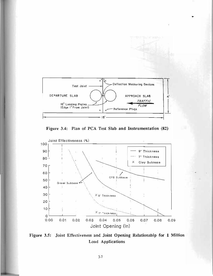
pavements. This study was conducted using an instrumented test slab shown in Figure 4 subjected

to a repetitive 9 kip load. The joint in the test slab was an induced crack from a metal strip 1 inch

in height placed at the pavement bottom and the top. During the repetitive loading, measurements

of joint opening and slab deflections on the loaded and unloaded slab were made at regular

intervals. The loading sequence across the joint was similar to a continous application of truck loads traveling approximately 30 mph. Test results in the form of joint effectiveness (EJ), joint

opening, and loading cycles for a 7 and a 9 inch slab thickness using a 6 inch gravel subbase were ..

shown previously in Figures 3.13a and b. The equation for joint effectiveness, given in Chapter

3, is similar to load transfer efficiency in that if the deflections on the loaded and unloaded slabs are equal then the joint effectiveness is 100 percent. (Note: the load transfer efficiency (LTE) is the

unloaded deflection divided by the loaded deflection, in percent.)

The results indicate the joint effectiveness tends to level off after about 700,000 to 800,000 load applications. The level of joint effectiveness at 1 million applications may provide a useful

basis relating joint or crack width to an ultimate joint effectiveness for design purposes. Figure 3.5

shows the change in the final joint effectiveness with the joint opening for the 7 and 9 inch

thicknesses. Some results were also obtained for other subbases types and are shown in Figure

3.5, which indicate that foundation strength can improve the load transfer performance. The

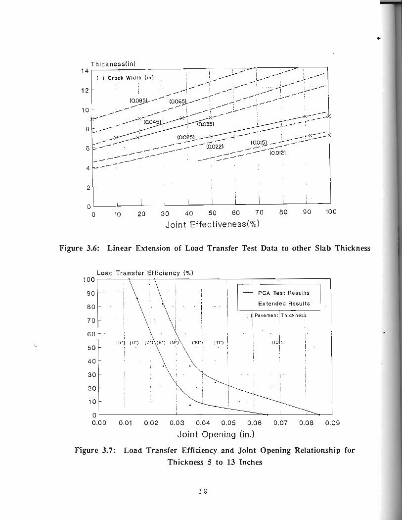
results from the 7 and 9 inch thicknesses are linearly extended to include other thicknesses (Figure

w

3.6 ). The joint effectiveness from the linear extensions was converted into load transfer efficiency

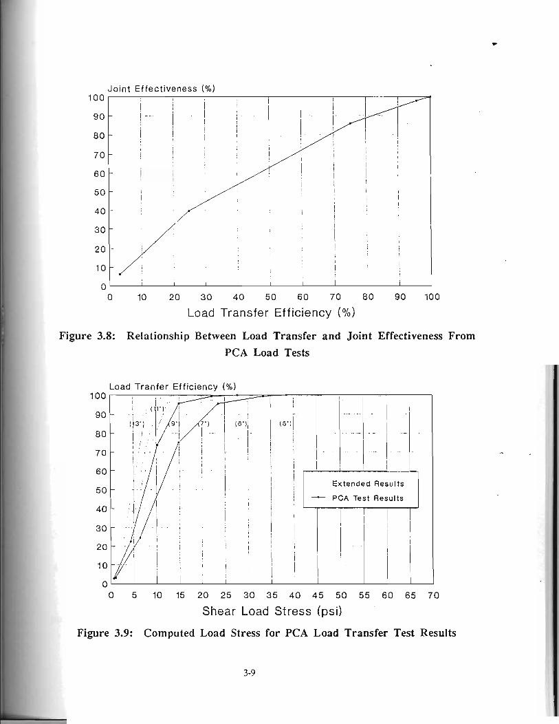
(L'IE) and replotted in Figure 3.7. The conversion process was aided by the use df Figure 3.8 which was a good approximation for the range of thicknesses shown in Figure 3.7. Further

laboratory tests and field studies should be conducted to validate the extrapolations made from the

PCA test data.

In order to extend the results of the PCA loads tests to other load conditions and pavement

configurations, load or shear stresses due to the aggregate interlock must be determined for the test

conditions. Using the load results directly is not reasonable since the laboratory loading conditions

are different from those in actual CRC pavement. This was mostly due to the width of the test

specimen, load position, and the height of the roughened interface where the aggregate interlock

functioned. All of these factors can be accounted for in the slab analysis model ELI-SLAB

described previously. This model allowed the load transferred by the aggregate interlock at each

node along the transverse crack to be determined. A node spacing of 6 inches was used to

determine the shear load. Using the average of smaller nodal spacing over the middle 6 inches

under the load position yielded results similar to the 6 inch nodal spacing. Modeling the test slab

with the ILLI-SLAB program yielded load stresses on the joint face for the test thicknesses plus the

range of thicknesses in which the load transfer data had been extended. These results are shown in

Figure 3.9. Using the ILLI-SLAB model, shear stresses can be found from other slab configurations,

such as CRC pavement with closely spaced cracking shown in Figure 3.10, and related to the test

slab conditions. A comparison of a bituminous shoulder and a two foot extended driving lane is

made in Figure 3.10 with the PCA test slab. An edge load position for the bituminous shoulder is

adjacent to the outer pavement edge where an edge load position for the extended driving lane is

two feet from the outer pavement edge. Greater shear stresses occur with a bituminous shoulder

condition. The edge loading of a bituminous shoulder with non-uniform support represents the .-

most severe loading conditions for shear stresses as would be expected. The non-uniform support

condition (illustrated in Figure 3.11) extended across the lane under the loaded slab in the ILLI-

SLAB model. The loading condition for a two foot extended driving lane is not as severe as the

loading conditions for the PCA test slab while a bituminous shoulder load condition with the rebar

contributing to the load transfer lowers the shear stress further. However, the later difference is

not as pronounced with LTErs greater than 90 percent. Little difference in shear stress is noted

between and interior load position (inner wheel path) and the edge load position with the extended

driving lane. Similar results were found between a ten foot tied concrete shoulder and the extended

driving lane. Figure 3.9 indicates the LTE for a given thickness and load stress that is input into

Figure 3.7 to determine the required joint opening (or crack width in the case of CRC pavements)

to maintain the given level of LTE for 1 million coverages. Using Figures 3.9 and 3.7, in that

- order, the corresponding limiting crack widths are found and illustrated in Figure 3.12. This

figure draws a comparison of edge loading between a bituminous shoulder and a two foot extended

driving lane with change in slab thickness at approximately a 95 percent LTE. This figure

describes a fundamental relationship between required or limiting crack width and pavement

thickness in terms of load transfer applicable to CRC thickness design.

CONE PULLOUT FRACTURE

1 DEFORMED BAR (

PRIMARY) LINTERNAL CRACK CRACK

SPALLING ON CRACK FACE

FRACTURE -42+

LOSS OF LOAD TRANSFER LONGITUDINAL CRACKING

q CRACKING

I m E

l I

I Figure 3.1: Failure Modes Related to Punchout Distress in CRC Pavement

Crack Spacing . -. . . . . Temperature Drop

Figure 5.2: Sensitivity of Steel Stress to Crack Spacing and Temperature Drop Using TTICRCP for 0.7 Percent Steel

Crack Spacing ( f t ) Temperature Drop (deg F) 10 80

- 70

8 -

), - 6 0

Load Transferred (Ibs) Compressive Strength (%)

2000 1 1100

6

4

2

0

...... Unsupported

Supported

0 I I I I I I I I ' I 0

0 . 10 20 30 40 50 60 70 80 90 100

Load Transfer Efficiency (05,)

16 18 2 0 22 2 4 2 6 28

Steel Stress (ksi)

- -

4 1 1 Crack Spacing ...,,' - 68 deg F Temp Drop

- -

- -

-

' I I I I I

Figure 33: Correlation Between Dowel Load and Maximum Bearing Capacity for No. 5 Bar

50

40

30

20

10

0

Test Joint Deflection Measuring Devices f

DEPARTURE SLAB APPROACH SLAB I 4'

TRAFF/C 16" Loading Plates (Edge I" From Joint) FLOW

.-Reference Plugs I Figure 3.4: Plan of PCA Test Slab and Instrumentation (82)

'0.00 0.01 0.02 0.03 0.04 0.05 0.06 0.07 0.08 0.09

Joint Opening (in)

Figure 3.5: Joint Effectiveness and Joint Opening Relationship for 1 Million Load Applications

- - - .. - - . . . . - -- rl

I

I

w

Thicknesdin) ~ 14 i ( 1 Crock width (In-) ,

12 -

I 10 -

/- -- -*- /- 4-

//-- / / A -

4

2

0 I I I I

0 10 20 30 40 50 60 70 80 90 100

Joint ~ f f e c t i v e n e s s ( % )

Figure 3.6: Linear Extension of Load Transfer Test Data to other Slab Thickness

Load Transfer Efficiency (%I

PCA Test Results

Extended Results

! '. .

I

0.00 0.01 0.02 0.03 0.04 0.05 0.06 0.07. 0.08 0.09

Joint Opening (in.)

Figure 3.7: Load Transfer Efficiency and Joint Opening Relationship for Thickness 5 to 13 Inches

I

3-8

I I

-/-A-

I

- I

1 I 1

I

I I

Joint Effectiveness (Oh)

0 10 20 30 40 50 60 70 80 90 100

Load Transfer Efficiency (%)

Figure 3.8: Relationship Between Load Transfer and Joint Effectiveness From PCA Load Tests

. . . -- . . - . -

Extended Results

PCA Test Results

Load Tranfer Efficiency (YO) 100

90

0 0 5 10 15 20 25 30 35 40 45 50 55 60 65 70

Shear Load Stress (psi)

Figure 3.9: Computed Load Stress for PCA Load Transfer Test Results

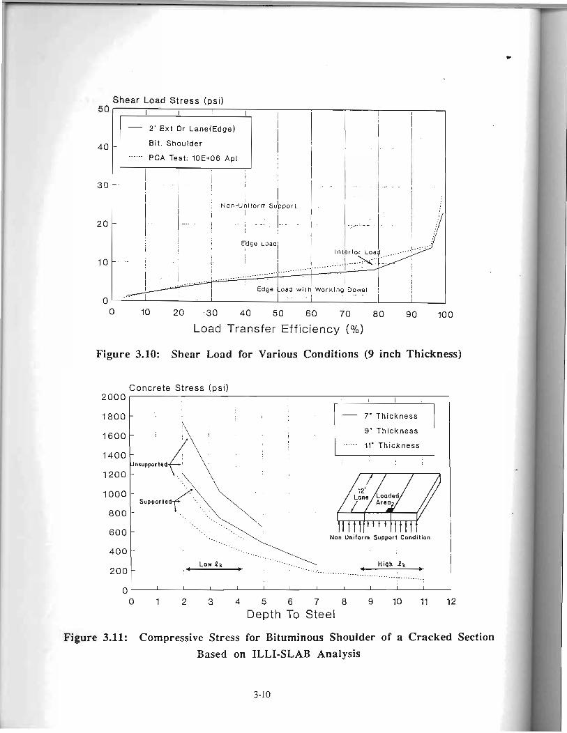
Shear Load Stress (psi)

0 10 20 -30 40 50 60 70 80 90 100

Load Transfer Efficiency

Figure 3.10: Shear Load for Various Conditions (9 inch Thickness)

Concrete Stress (psi) 2000 1 I I

f I

! ( - 7. Thickness I I I

9' Thickness I

I I .....- 11' Thickness

1400 o o ~ n s u p p o r + e d ~ / ' I

. . . Non Uniform Support Condition

High i k +

.....................................

0 [ I I I I 1 I I I I I I

0 1 2 3 4 5 6 7 8 9 1 0 1 1 1 2 Depth To Steel

Figure 3.11: Compressive Stress for Bituminous Shoulder of a Cracked Section Based on ILLI-SLAB Analysis

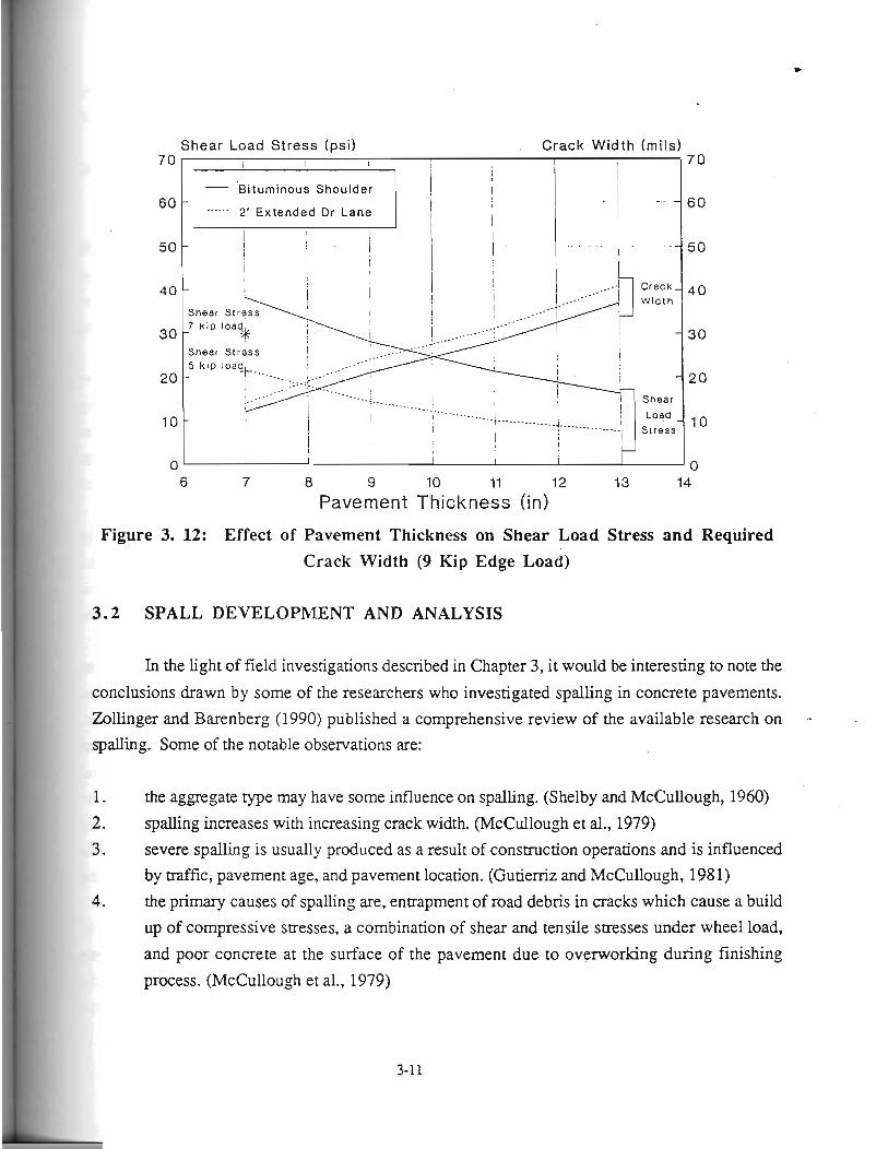
Shear Load Stress (psi) Crack Width (mils) 7 0 i I I I I 70

I I 1 i i I

Bituminous Shoulder

2' Extended Dr Lane

........ ........... Load ................ 10 - I"-- ; I I i

I i !

0 I I I I I I I 0

Pavement Thickness (in)

Figure 3. 12: Effect of Pavement Thickness on Shear Load Stress and Required Crack Width (9 Kip Edge Load)

3 .2 SPALL DEVELOPMENT AND ANALYSIS

In the light of field investigations described in Chapter 3, it would be interesting to note the

conclusions drawn by some of the researchers who investigated spalling in concrete pavements.

Zollinger and Barenberg (1990) published a comprehensive review of the available research on .-

~palling. Some of the notable observations are:

1. the ag,gegate type may have some influence on spalling. (Shelby and McCullough, 1960)

2. spalling increases with increasing crack width. (McCullough et al., 1979) 3. severe spalling is usually produced as a result of construction operations and is influenced

by traffic, pavement age, and pavement location. (Gutieniz and McCullough, 1981)

4. the primary causes of spalling are, entrapment of road debris in cracks which cause a build

up of compressive stresses, a combination of shear and tensile stresses under wheel load,

and poor concrete at the surface of the pavement due to overworking during finishing

process. (McCullough et al., 1979)

I

5 . deeper spalls are generally related to structural weaknesses whereas shallow and wide

spalls are related to weakened, horizontal planes in the surface of concrete. (NCHRP

Synthesis 60, 1979)

6 . spalling over reinforcement is not considered to be a widespread problem in CRC

pavements. (Zollinger and Barenberg, 1990)

In addition to the above, results from the analysis performed by Tayabji and Colley (1988)

indicated that increased restraint at the cracks or joints increases the compressive smsses at the top

of the slab, and also that a differential temperature distribution results in lower tensile stresses at

the bottom of the slab as a result of restraint from the subgrade. These results are very important

indicators of the factors involved in the spalling mechanism.

Based on our field surveys, we have substantial evidence to show that the concrete pavement delaminates at a very early age and these delaminations eventually deteriorate to spalling

due to the action of stresses caused by temperature effects, wheel loads and subgrade effects.

Therefore, we consider that it is important to investigate the state of the concrete at a very early age

prior to the application of a significant number of cycles of temperature related stresses and stresses

from wheel loads.

Zollinger and Barenberg (1990) showed from their analysis that their is a relationship

between the crack width and spalling in CRC pavements, thus substantiating the observations

made by Shelby and McCullough (1960). This emphasizes the importance of the prediction of the

crack pattern. Mechanistic methods such as the TlTCRCP computer program predicts crack pattern

for CRC pavements over a specified analysis period

A number of computer programs have been developed over the years which attempt to

model the behavior of CRC pavements. The TTICRCP computer program is one such program.

It includes models for subgrade friction, bond stress of reinforcement, and concrete shrinkage. ..

This program calculates the stresses in the concrete mass induced by shrinkage and restraint from

subbase friction and reinforcement. It calculates the stress state in the pavement including the bond

stress of reinforcement and the friction stress from subbase along the longitudinal direction of the

pavement. Being a program which was primarily developed for crack prediction, it does not

consider the differential shrinkage across the depth of the pavement. However, to model the

phenomenon of delamination, we must be able to model differential shrinkage of the concrete

pavement across its depth.

The work done by Bazant and Najjar (1977) to model such shrinkage is very significant in

this regard. Work is under way at the Texas Transportation Institute to develop a finite element

computer program which includes this model to calculate changes in pore humidity with time in

unsaturated media. This computer program models changes in pore moisture due to variations in

*

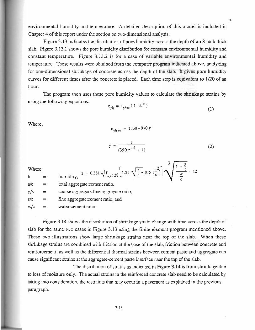
environmental humidity and temperature. A detailed description of this model is included in

Chapter 4 of this report under the section on two-dimensional analysis.

Figure 3.13 indicates the distribution of pore humidity across the depth of an 8 inch thick

slab. Figure 3.13.1 shows the pore humidity distribution for constant environmentd humidity and

constant temperature. Figure 3.13.2 is for a case of variable environmental humidity and

temperature. These results were obtained from the computer program indicated above, analyzing

for one-dimensional shrinkage of concrete across the depth of the slab. It gives pore humidity

curves for different times after the concrete is placed. Each time step is equivalent to 1/20 of an

hour.

The program then uses these pore humidity values to calculate the shrinkage strains by

using the following equations.

Where, 'sh = = 1330 - 970 y

a/c = total aggregate:cement ratio,

g/s = coarse aggregate:fine aggregate ratio, s/c = fme aggregate:cement ratio, and w/c = watexcement ratio.

Figure 3.14 shows the distribution of shrinkage strain change with time across the depth of

slab for the same two cases in Figure 3.13 using the finite element program mentioned above. I These two illustrations show large shrinkage strains near the top of the slab. When these

shrinkage strains are combined with friction at the base of the slab, friction between concrete and

reinforcement, as well as the differential thermal strains between cement paste and aggregate can

cause significant strains at the aggregate-cement paste interface near the top of the slab.

The distribution of strains as indicated in Figure 3.14 is from shrinkage due

to loss of moisture only. The actual strains in the reinforced concrete slab need to be calculated by

taking into consideration, the restraints that may occur in a pavement as explained in the previous

paragraph.

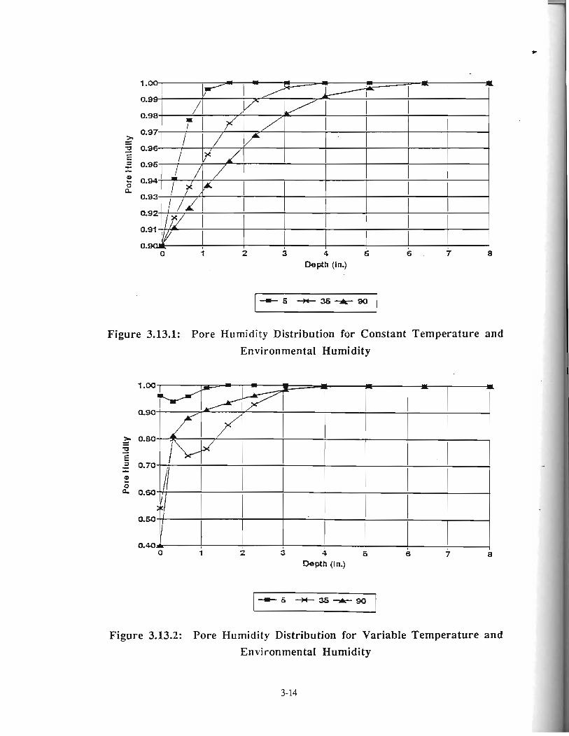
> = -U 0.96 - /

E 1 0.96- - I 2 0.94 0 a Mi

I r - I 0.93 / f i r I-- ay I I

I 0.91

0. 1 0 2 3 4 6 6 7 8

I

Depth (In.)

Figure 3.13.1: Pore Humidity Distribution for Constant Temperature and

Environmental Humidity

Depth (In.)

Figure 3.13.2: Pore Humidity Distribution for Variable Temperature and Environmental Humidity

*

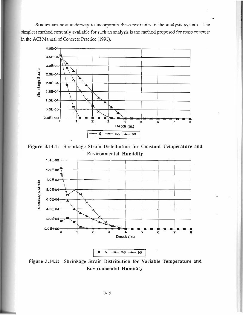
Studies are now underway to incorporate these restraints to the analysis system. The

simplest method currently available for such an analysis is the method proposed for mass concrete

in the ACI Manual of Concrete Practice (1991).

Depth (In.)

Depth (in.)

Figure 3.14.1: Shrinkage Strain Distribution for Constant Temperature and Environmental Humidity

Figure 3.14.2: Shrinkage Strain Distribution for Variable Temperature and Environmental Humidity

er,

I I

1 0 6 6 7 8

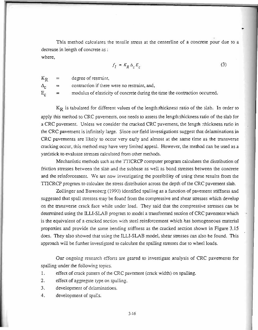
This method calculates the tensile stress at the centerline of a concrete pour due to a

decrease in length of concrete as :

where,

fi = KR Ac Ec

- K~ - degree of restraint,

4 = contraction if there were no restraint, and,

Ec = modulus of elasticity of concrete during the time the contraction occurred.

KR is tabulated for different values of the 1ength:thickness ratio of the slab. In order to

apply this method to CRC pavements, one needs to assess the 1ength:thickness ratio of the slab for

a CRC pavement. Unless we consider the cracked CRC pavement, the length :thickness ratio in

the CRC pavement is infinitely large. Since our field investigations suggest that delaminations in

CRC pavements are likely to occur very early and almost at the same time as the transverse

cracking occur, this method may have very limited appeal. However, the method can be used as a

yardstick to evaluate messes calculated from other methods.

Mechanistic methods such as the TT'ICRCP computer program calculates the dismbution of friction stresses between the slab and the subbase as well as bond suesses between the concrete

and the reinforcement. We are now investigating the possibility of using these results from the

TI'ICRCP program to calculate the stress distribution across the depth of the CRC pavement slab.

Zollinger and Barenberg (1990) identified spalling as a function of pavement stiffness and

suggested that spa11 stresses may be found from the compressive and shear stresses which develop

on the transverse crack face while under load. They said that the compressive stresses can be

determined using the ILLI-SLAB program to model a transformed section of CRC pavement which

is the equivalent of a cracked section with steel reinforcement which has homogeneous material

properties and provide the same bending stiffness as the cracked section shown in Figure 3.15 does. They also showed that using the ILLI-SLAB model, shear stresses can also be found. This

approach will be further investigated to calculate the spalling stresses due to wheel loads.

Our ongoing research efforts are geared to investigate analysis of CRC pavements for

spding under the following topics.

1. effect of crack pattern of the CRC pavement (crack width) on spalling.

2. effect of aggregate type on spalling.

3. development of delaminntions.

4. development of spalls.

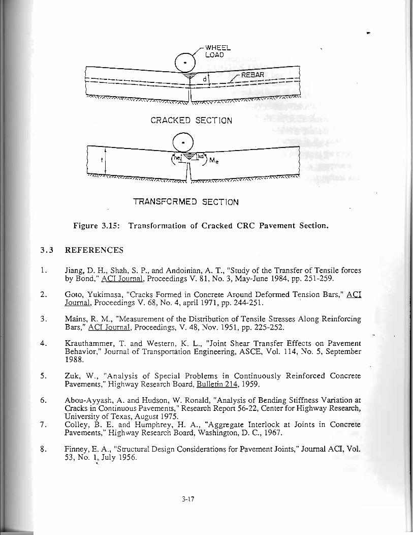
WHEEL p(- LOAD

CRACKED SECTION

TRANSFORMED SECTION *

Figure 3.15: Transformation of Cracked CRC Pavement Section.

3 . 3 REFERENCES

1. Jiang, D. H., Shah, S. P., and Andoinian, A. T., "Study of the Transfer of Tensile forces by Bond," ACT Journal, Proceedings V. 81, No. 3, May-June 1984, pp. 251-259.

2. Goto, Yukimasa, "Cracks Formed in Concrete Around Deformed Tension Bars," ACI Journal, Proceedings V. 68, No. 4, april 1971, pp. 244-251.

3. Mains, R. M., "Measurement of the Distribution of Tensile Stresses Along Reinforcing Bars," ACT Journal, Proceedings, V. 48, Nov. 1951, pp. 225-252.

4. Krauthammer, T. and Western, K. L., "Joint Shear Transfer Effects on Pavement Behavior," Journal of Transportation Engineering, ASCE, Vol. 114, No. 5, September 1988.

5. Zuk, W., "Analysis of Special Problems in Continuously Reinforced Concrete Pavements," Highway Research Board, Bulletin 214, 1959.

6. Abou-Ayyash, A. and Hudson, W. Ronald, "Analysis of Bending Stiffness Variation at Cracks in Continuous Pavements," Research Report 56-22, Center for Highway Research, University of Texas, August 1975.

7. Colley, B. E. and Humphrey, H. A., "Aggregate Interlock at Joints in Concrete Pavements," Highway Research Board, Washington, D. C., 1967.

8. Finney, E. A., "Structural Design Considerations for Pavement Joints," Journal ACI, Vol. 53, No. 1,. July 1956.

%.

* Tabatabaie, A. M., Barenberg, E. J., and Smith, R. E., "Volume I1 -- analysis of Load Transfer Systems for Concrete Pavements," Report No. FAA-RD-79-4, U. S: Department of Transportation, Washington, D. C., November 1979.

Yoder, E. J. and Witczak, M. W., Princi~les of Pavement Design, 2nd Edition, John Wiley and Sons, 1975.

Tayabji, S.D. and Colley, B.E., "Improved Rigid Pavement Joints", Research Report

FHWA/RD-86/040, Construction Technology laboratories, A Division of Portland Cement

Association, Skokie, Illinois, February 1986.

Bazant, Z.P. and Najjar, L.J., "Nonlinear Water Diffusion in Non-Saturated Concrete",

Materials and Structures, Vol. 5, No. 25, 1972, Paris.

Kadiyala, S.M., "Study of Factors Affecting the Formation of Cracks in Continuously

Reinforced Concrete Pavements," Master's Thesis to be Published, Department of Civil

Engineering, Texas A & M University, College Station, Texas, December, 1991.

ACI Manual of Concrete Practice, Part 1, Materials and general Properties of Concrete,

1991. +

Palmer, R.P., Olsen, M.P.J., and Lytton, R.L. "TTICRCP - A Mechanistic Model for the

Prediction of Stresses, Strains, and Displacements in Continuously Reinforced Concrete

Pavements", Research Report No. FHWAjTX-881371-2F, Texas State Department of

Highways and Public Transportation, Texas Transportation Institute, College Station,

Texas, July 1988.

Zollinger, D.G., and Barenberg, E.J., "Continuously Reinforced Pavements : Punchouts i I and other Distresses and Implications for Design", Research Report No. FHWAEAJI

227, Illinois Dep'mment of Transportation, Department of Civil Engineering, Engineering

Experiment Station, University of Illinois, Urbana, March 1990.

Shelby, M.D. and McCullough, B.F., "Experience in Texas with Continuously Reinforced I

Concrete Pavement," Bulletin 274, Highway Research Board, 1960.

McCullough, B.F., Ma, J.C.M., and Noble, C.S., "Limiting Criteria for The Design of , I

CRCP," Research Report 177- 17, The Center for Transportation Research, University of . I

I

Texas, August 1979.

Gutiemz de Veiasco, M. and McCullough, B.F., "Summary Report for 1978 CRCP

Condition Survey in Texas," Research Report 177-20, center for Transportation Research,

University of Texas, January 198 1.

NCHRP, "Failure and Repair of Continuously Reinforced Concrete Pavement," NCHRP

Synthesis 60, July 1979.

CHAPTER 4

CRACK CONTROL METHODOLOGIES OF CRCP AND JCP

Due to deep sawcuts which occasionally extended beyond the level of the transverse steel to

form the longitudinal joint and the occurrence of random longitudinal cracking (Figure 4.1)

experienced on past construction projects have lead to interest in the development of methodology

to minimize these problems. Therefore, work has been underway to investigate techniques both in

the past and present to improve the practice of crack control. Improvement in the control of

cracking in concrete pavements actually involves certain construction phases relating to the method

of curing and the timing of saw cutting operations. Crack control in this study is interpreted to

apply to PCC pavements in general, both jointed and CRC pavements, both longitudinal and

transverse joints.

Crack control can even apply to the crack pattern in CRC pavement. There are several

reasons to literally control the crack pattern in CRC pavement. Probably the most prevalent is the

obvious potential benefit from achieving a set crack pattern which demonstrates a minimal

deviation in crack spacing and practically no crack randomness. Other very important reasons

pertain to minimizing or limiting the development of Y-cracking in the crack pattern. Cracking

features such as these have a tendency to develop into punchouts. Another reason is to reduce the

occurrence of deep spalls due to irregular cracking at the surface of the pavement. Pavement

spalling will be discussed momentarily but a very important aspect of a controlled crack pattern in

CRC pavement is the minimization of undesirable crack intervals (Figure 4.2) and punchouts

(Figure 4.3) providing the ability of the design engineer to achieve an equivalent design for any

aggregate type based on the added control afforded the design process. It should be possible to

choose the same amount of steel for design and achieve equivalent designs for any aggregate by --

forming the crack pattern to achieve the appropriate crack widths to provide the same level of

performance.

Past and present performance data justifies a more in-depth study of the effect of different

aggregate types on the slab behavior under environmental and traffic load and the effect that

construction methodolo,3r may have. A method of achieving equal performance between any type I of coarse aggregate may then be achieved by forming the crack pattern with respect to each

aggregate type which will yield crack widths that will produce that same level of performance I between aggregate types. Input from the aggregate producers and construction industry has I

proven to be useful in the development of this construction methodology.

Crack control methodology has been considered previously in 1969 on test sections

constructed in Houston (on the west bound frontage road of IH-610 South Loop near Wayside).

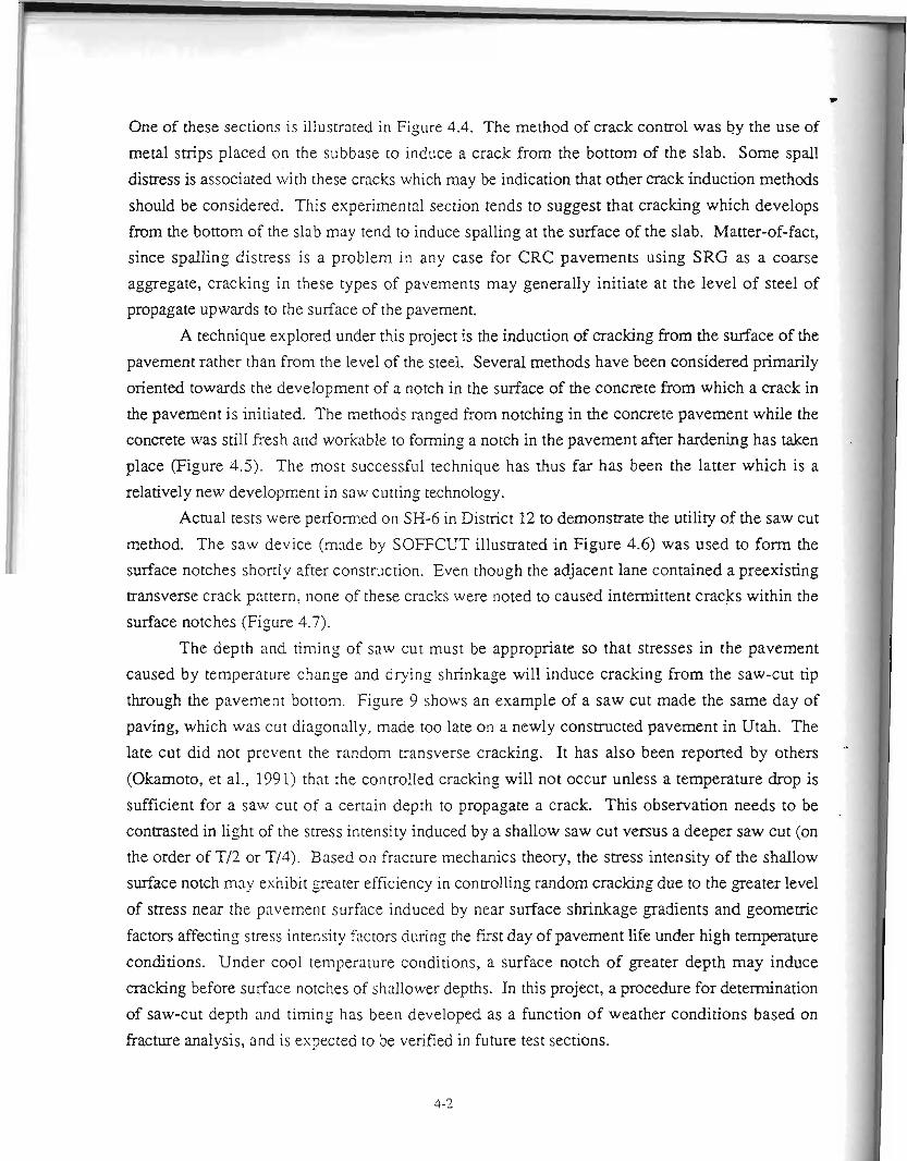
One of these sections is illustrated in Figure 4.4. The method of crack control was by the use of

metal strips placed on the subbase to induce a crack from the bottom of the slab. Some spa11

distress is associated with these cracks which may be indication that other crack induction methods

should be considered. This experimental section tends to suggest that cracking which develops

from the bottom of the slab may tend to induce spalling at the surface of the slab. Matter-of-fact,

since spalling distress is a problem in any case for CRC pavements using SRG as a coarse

aggregate, cracking in these types of pavements may generally initiate at the level of steel of

propagate upwards to the surface of the pavement.

A technique explored under this project is the induction of cracking from the surface of the

pavement rather than from the level of the steel. Several methods have been considered primarily

oriented towards the development of a notch in the surface of the concrete from which a crack in

the pavement is initiated. The methods ranged from notching in the concrete pavement while the

concrete was still fresh and workable to forming a notch in the pavement after hardening has taken

place (Figure 4.5). The most successful technique has thus far has been the latter which is a

relatively new development in saw cutting technology.

Actual tests were perfomled on SH-6 in District 12 to demonstrate the utility of the saw cut

method. The saw device (made by SOFFCUT illustrated in Figure 4.6) was used to form the

surface notches shortly after construction. Even though the adjacent lane contained a preexisting

transverse crack pattern, none of these cracks were noted to caused intermittent cracks within the

surface notches (Figure 4.7).

The depth and timing of saw cut must be appropriate so that stresses in the pavement

caused by temperature change and drying shrinkage will induce cracking from the saw-cut tip

through the pavement bottom. Figure 9 shows an example of a saw cut made the same day of

paving, which was cut diagonally, made too late on a newly constructed pavement in Utah. The

late cut did not prevent the random transverse cracking. It has also been reported by others "

(Okamoto, et al., 1991) that the controlled cracking will not occur unless a temperature drop is

sufficient for a saw cut of a certain depth to propagate a crack. This observation needs to be

contrasted in light of the stress intensity induced by a shallow saw cut versus a deeper saw cut (on

the order of Ti2 or T/4). Based on fracture mechanics theory, the stress intensity of the shallow

surface notch may eshibit greater efficiency in controlling random cracking due to the greater level

of stress near the pavement surface induced by near surface shrinkage gradients and geomemc

factors affecting stress intensity factors during the first day of pavement life under high temperature

conditions. Under cool temperature conditions, a surface notch of greater depth may induce

cracking before surface notches of shallower depths. In this project, a procedure for determination

of saw-cut depth and timing has been developed as a function of weather conditions based on

fracture analysis, and is expected to be verified in future test sections.

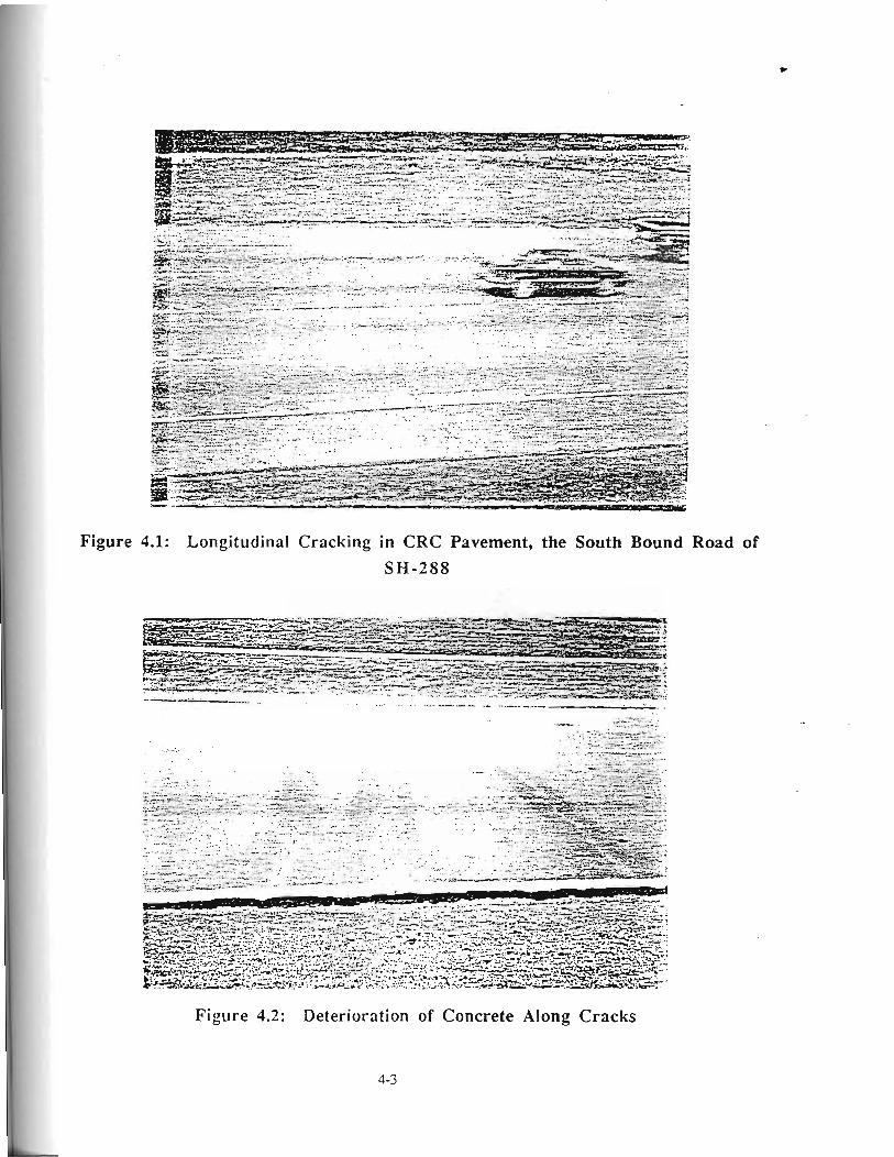
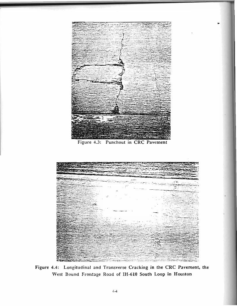
Figure 4.3: Punchout in CRC Pavement

Figure 4.4: Longitudinal and Transverse Cracking in the CRC Pavement, the West Bound Frontage Road of IH-610 South Loop in Houston

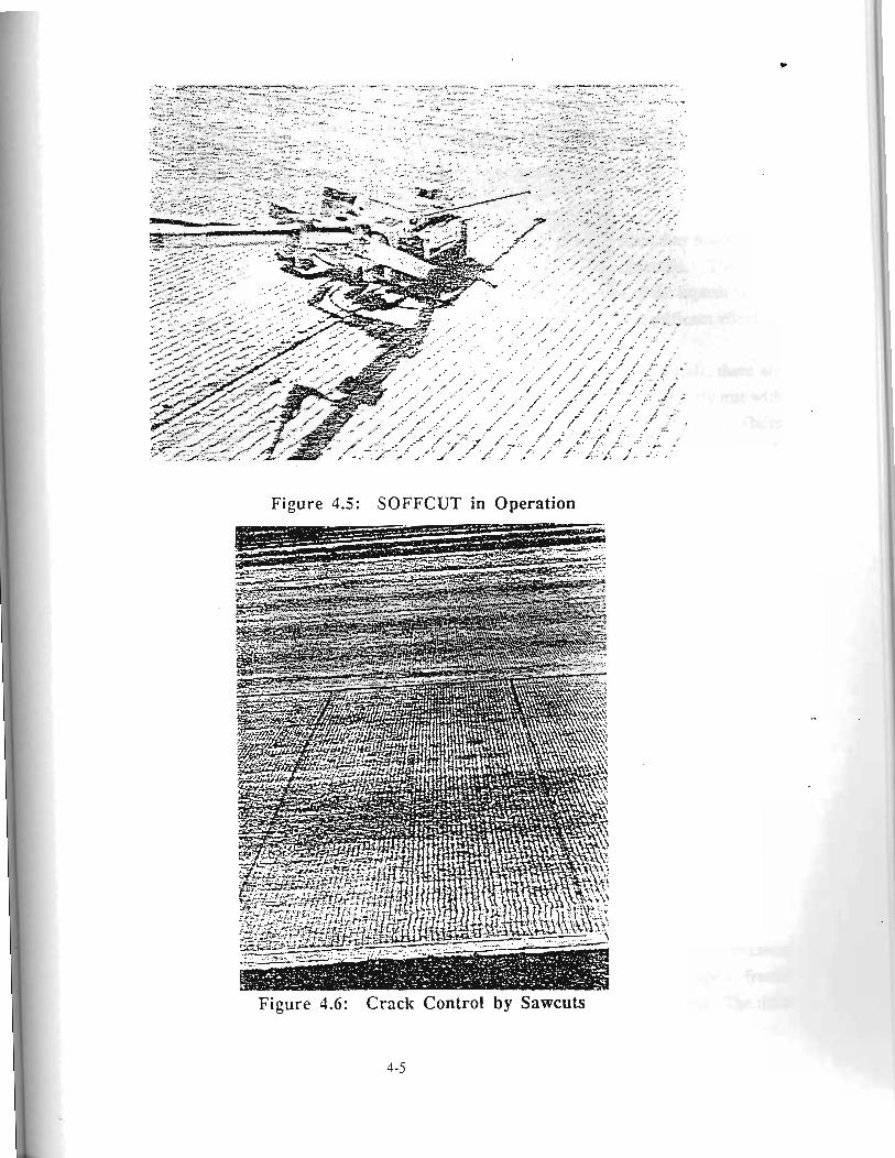
S-P

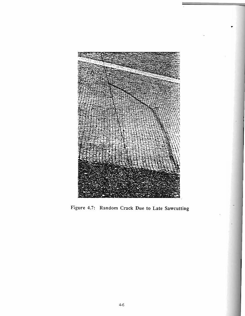
Figure 4.7: Random Crack Due to Late Sawcutting

CHAPTER 5

AGGREGATE SHAPE CHARACTERIZATION WITH FRACTALS

5.1 BACKGROUND AND INTRODUCTION

Mineral aggregates are critical components of construction material, since they make up the

major portion of weight in bituminous or concrete paving mixture materials. Thus, the characteristics of mineral aggegates can influence the structural performance of the asphalt paving

material. Many researchers have shown that the aggregate properties have a significant effect on

the performance of the construction materials (5.1-5.8)

As important as aggregates are to the performance of construction materials, there are

relatively few methods to quantify their contributions to performance. This is particularly true with

respect to the surface characteristics such as particle shape, roughness and surface charge. Those

attributes are important to the interaction between the aggregates and the binder in the material.

Unfortunately, the information provided by most tests today on ageoregate shape and texture are

only categorically and subjective.

Fractals embody new mathematical tools and image processing techniques which are used

to describe natural structure that are irregular, rough or fragmented. Fractals have been

successfully applied in the fields of medicine, metallurgy, geology and material science (5.9-5.17).

Also, fractals can quantitatively describe the geometric irregularity of aggregate particles.

Preliminary work at TTI in HP&R Study 1121, "Investigation of Rutting in Asphalt Pavements,"

indicates that fractals can truly provide very sensitive measurements of aggregate shapes (from

clusters or single stones). The calculated fractal dimensions for river gravel and crushed limestone

are 2.34 and 2.46 respectively. (See Figures 5.1 & 5.2 and Tables 5.1 & 5.2.) This indicates the ..

crushed limestone has sharp edge and rough texture when compared with river gravel.

Our team has also conducted research in the area of biological organ modeling with fractals

(5.13). Figure 5.3 shows two examples of how the muscular texture of the heart is retained with -

the calculated fractal dimension despite a series of magnification. This technique can be used to

evaluate the texture of aggegste surface.

5.2 OBJECTIVE OF THE RESEARCH TASKS

This research task outlines methods to provide a quantitative and objective characterization

of aggregates. The first objective is to quantify the aggregate shape with the concept of fractal I dimension. The second objective is to quantify surface texture with fractal analysis. The third

* I

objective provides a measure to differentiate between cubical and plate-like aggregates. The fourth

I objective is to measure the color (greylevel) of the aggregates.

I 5.3 DESCRIPTION OF ANALYSIS PROCEDURE

5.3.1. Shape (Angularity) Measure

The aggregate shape analysis is divided into three parts. The first part is edge extraction or

contour extraction. The second part is called Slope Density Function and the last part is called

Fractal boxcount. aggregate is first recorded with a high-resolution video camera on Super VHS video tape. The aggregate video picture is then digitized into 512 x 480 picture elements (pixels).

Each element has a greyscale range from 0 to 255. "0" usually indicates completely dark while

"255" represents the brightest level.

5.3.1.1. Edge Extraction

The edge extraction algorithm starts with a horizontal scan that intersects with an edge

picture element (pixel). The subsequent senrch for neighboring pixel will follow these basic rules.

There are eight search directions, nanlely, N, NE, E, SE, S, SW, W, NW. The algorithm keeps

account of the previous search direction. It will first "reset" the direction at two steps in counter

clockwise direction from previous search. It then will research in clockwise direction one step at a

time until the next connecting pixel is found. This search will continue until it finishes traversing

the edge of the aggregate and returns to the starting point. The locations of all the edge pixels are

stored for future calculation. Figures 5.4 and 5.5 illustrate the edge (shape) of a Crushed

Limestone Aggregate and a River Gravel, respectively. The discontinuous line is due to the fact

that the printer prints every other ROW and COLUMN.

5.3.1.2 Slope Density Function (SDF) The "running" slope is calculated based on the locations (coordinate pairs) of the edge

pixels. A slope or the angle (Y) of the line connected by the 1st and the 4th pixels is frst calculated -

for each pixel (See Figure 5.6). The Slope Density Function is the frequency dismbution of each

slope (angle). A jagged SDF curve indicates an angular shape while a smooth SDF curve

represents a "rounded" shape. Figure 5.7 illilstrates the SDF curve for a square box. The four

peaks correspond to four sides of the square, with slope angle equal to 90°, 180°, 270°, and 360'.

Figure 5.8 illustrates the SDF curve of n circle. Ideally, the SDF curve for a circle is a smooth

horizontal line since the slope angle or the tangent to the circumference will include all possible

360'. The observed '.jaggedu curve is due to the imperfect digitization and representation of a circle with square pixels. This situation can be improved with higher resolution video recording and

digitization equipment such as the 1024 x 1024 pixels format. Figures 5.9 and 5.10 illustrate a

'C

Crushed Limestone aggregate and River Gravel aggregate with their corresponding SDF curve,

respectively. The SDF curve of Crushed Limestone aggregate has multiple larger peaks which

represent longer straight edges and. more sharp corners (more angular) when compared with River

Gravel.

5.3.1.3 Fractal Boxcount

The Fractal Boxcoi~nt technique aims to compute the fractal dimension (F.D.) for the SDF

curve. This technique starts with a uniform g id pattern overlaid with the SDF curve. The grid

pattern or the box size (b) is then changed, and the number of boxes (N) which contained a line

segment is counted. Their fi~nctional relationship can be described as in equation (1).

As the box size decreases, the number of boxes which contains line segment also increases.

The rate of increase is larger for jagged curve than for smooth curve. The slope of the Log-Log

plot of the number of non-emptied boxes versus box size is the Fractal Dimension (F.D.) of the

SDF curve. A higher F.D. represents a jagged SDF curve which in turn implies an angular

aggregate. Figure 5.1 1 illustrrites the Fractal boxcount curves for the square and the circle. It can

be observed that the slope for the Fractal boscount curve is larger for the square than for the circle.

This is in agreement with the fact that a larger slope indicates a more angular shape of an object.

Figure 5.12 illustrates a pair of Fractal boxcount curves for Crushed Limestone and River Gravel.

As expected, the slope for the Crushed Limestone curve is steeper than that of the River Gravel. A

larger shape (angular) measure represents a more angular aggregate.

5.3.2. Silrface Texture As discussed in the previous sections, the greylevel of each picture element in the digitized

picture of aggregate surface represents the lightfdark shade of the picture element. Under

appropriate light condition, the degree of brightness/darkness relates to the profile of the picture -

element. In other words, a bright greylevel associates with a peak while a dark greylevel

associates with a valley on the aggregate surface.

Fractal surface texture measure describes the variations of the greylevels within an area of

interest. A large variation indicates a rough texture and a small variation shows a smooth texture.

This functional relationship can be described with the following equations.

1-g lo;; url VULU d e s of the equation, the equation can be rewritten as:

log E [ I f(x + Ax) - f(x) I ] - H log I Ax I = log C (3)

- where f(x) is the greylevel at position x = (x,y) coordinate pair, H is the surface texture measure

and C is the mean of the distribution of the greylevels. I

The surface texture parameter H is the slope of the log E [f(x+A) - f(x)] versus log I Ax I

plot. The team employed a set of texture images for calibration and verification of the fractal

algorithm. The images used range from smooth to rough texture. Figure 5.13.1 shows a smooth

cardboard paper surface while Figure 5.13.2 is an image of a cork particle board surface and

Figure 5.13.3 is an image of n rough carpet surface. The corresponding texture parameter (H) is

computed to be 2.10,2.18, and 2.40 for cardboard, cork, and carpet, respectively. Two aggregate

examples are shown here in Figure 5.14 and Figure 5.15 to illustrate results from a Redland I I

. I Melendy CLS and a Gifford Hill Wardlaw SRG aggregates. A large H value indicates a rough

texture as for Redland Melendy CLS.

5.3.3. Elongation ~~~~~~~e Elongation measure provides n relative measure of the shape of an aggregate. This is

especially effective to differentiate between a cubical and a plate-like aggregate. This parameter

measures the major axis and the average minor axis. The average minor axis is calculated from the

area of the aggegate divided by its major axis. From the ratio of the major axis over the average minor axis, one can obtain an elongation measure. An example of a Vulcan Brownwood CLS and

Thorstenburg SRG are shown in Figures 5.16 and 5.17. The Vulcan Brownwood CL has a

higher elongation ratio since the aggregates are more plate-like.

5.3.4. Greylevel

The average greylevel gives an indication of the color of the aggregates. A high greylevel -

represents light color aggregates and vice versa. The average greylevel measured here is from a

pan of aggregates.

5 .4 DISCUSSION OF RESULTS

The shape measiire or angularity measure can divide the siliceous river gravels and the

crushed limestones where the later are more angular (See Table 5.3). The texture can further differentiate the river gravels and crushed stones by the higher value in the group of crushed

stones. An exception shows in Pioneer Gnrwood SRG where the aggregates are crushed and

w natural color dots shown on the aggregates' surfaces. The elongation measure, which is based on

the boundary geometry of an aggregxte, successfully classifies the rounded river gravels from the

crushed stones. Furthermore, this measure can also be used to find out the ratio of cubical and

plate-like aggregates within one type of aggregate. The average greylevel measure is useful to

differentiate dark color aggregate from light color as shown in the case of Redland Melendy CL

and Vulcan Brownwood CL.

The Fractal based shape (angularity) and texture measure along with traditional image

processing measures result in objective and comprehensive aggregate classification system.

5.5 RECOMMENDATION FOR FUTURE RESEARCH i

As discussed in the surface testure section, it is critical to measure the true surface profile

of the aggregate for texture analysis. The team recommends to investigate a laser range sensor to

give true surface profile. This will overcome the current visual measure where the color dots can

affect the interpretation of the surface roughness. Acquisition of three-dimensional image (volume

tendering) will give a true shape of an agregate, and improve over the single projection technique

used in the current aggregate classification system.

5 .6 REFERENCES

5.1 E. R. Hargett, "Effects of Size, Surface Texture, and Slope of Aggregate Particles on the

Properties of Bituminous Mistures," Special Report 109, HRB, National Research

Council, Washington, D.C., 1970, p.25.

5.2 F. J. Benson, "Effects of Aggregate Size, Shape, and Surface Texture on the Properties of

Bituminous Mixtures: A Literature Survey," Special Report 109, HRB, National Research

Council, Washington, D.C., 1970, pp. 12-21.

5.3 M. Lineh and J. Greenstein, "Influence of Aggregate Shape on Engineering Properties of

Asphaltic Paving Mistures," 111 Highway Research Board 404, HRB, National Research

Council, Washington, D.C., 1972, pp. 42-56.

5.4 C. L. Monismith, "Influence of Shape, Size, and Surface Texture on the Stiffness and

Fatigue Response of Asphalt A<ixtures," Special Report 109, HRB, National Research

Council, Washington, D.C., 1970, pp. 4-11.

w 5.5 J. M. Griffith and B. F. Dallas, "Intluence of Fine Aggregates on Asphaltic Concrete

Paving Mixtures," H R B Proc., Vol. 37, 1958, pp. 219-255.

5.6 W. C. Krumbein, "Measurement and Geological Significance of Shape and Roundness of

Sedimentary Particles," Journal of Sedimentary Petrology, Vol. 13, No. 2, Aug. 1941, pp.

64-72.

5.7 G. Rittenhouse, "A Visual Method of Estimating Two Dimensional Sphericity," Journal of

Sedimentary Petrology, Vol. 13, No. 2, Aug. 1941, pp. 79-81.

5.8 B. Mather, "Shape, Surface Texture, and Coatings of Aggregates," Misc. Paper No. 6-

710. U.S . Army Corps of Engineers, Waterways Experiment Station, Vicksburg, Miss.,

Feb. 1965.

5.9 Bassingthwaighte, J. B.; van Beek, J. H. G. M., "Lightning and the Heart: Fractal

Behavior in Cardiac Function," Proc. IEEE 76:693-699; 1988.

5.10 Bassingthwaighte, J. B.; King, R. B.; Roger, S. A., "Fractal Nature of Regional

Myocardial Blood Flow Heterogeneity," Circ. Res. 65:578-590; 1989

5.1 1 C. C. Chen et. nl, "Fractal Fe:lture Analysis and Classification in Medical Imaging," IEEE

MI-8, NO. 2, pp. 133-142, 1989.

5.12 A. A. Tsonis, P. A. Tsonis, "Fractals; A New Look at Biological Shape and Patterning,"

Perspective in Biology and Medicine, 30: 355-361, Spring, 1987.

5.13. Lan Li, R. A. Robb, Paul Chan, R. L. Lytton, "Fractal Analysis and Application to

Biological Organ Modeling," 12th Int. Conf., IEEE Eng. in Medicine and Biology Society, -

Philadelphia, Pennsylvania, Nov. 1-4, 1990.

5.14 H. Nakaya~~irl, IM. Sone, 2nd iM. Takag, "Texture Analysis of Meteorological Image by

Fractals Dimension and Lower Order Statistics," Technical Report of IPS Japan, CV 44-4,

Sept. 1986.

5.15 B. B. Mandelbrot, D. E. Pnssoja, and A. J. Paullay, "Fractal Character of Fracture

Surfaces of RIIetals," Nr~ti~re, Vol. 308, 19, April, 1984.

I)

5.16 T. Chelidze, Y. Gueguen, " Evidence of Fractal Fracture," Int. J. Rock Mech. Min. Sci.

Geomech. Vol. 27, No. 3, pp. 223-225, 1990.

5.17 J. W. Martin, D. P. Bentz, "Fractal-Based of the Roughness of Blasted Steel Panels,"

Journal of Coatings Technology 59, pp. 35-41, Feb. 1987.

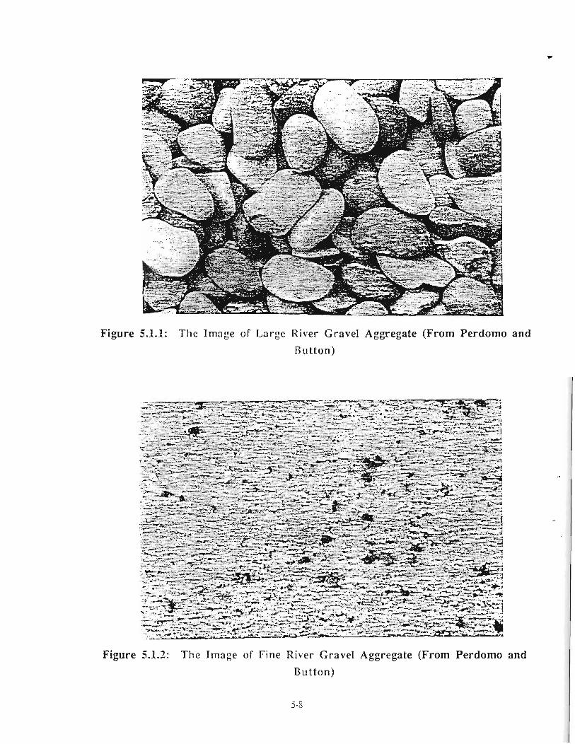
Figure 5.1.1: Tlie Image of Large River Gravel Aggregate (From Perdomo and Button)

Figure 5.1.2: The Tmnge of Fine River Gravel Aggregate (From Perdomo and Button)

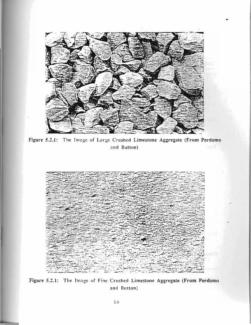
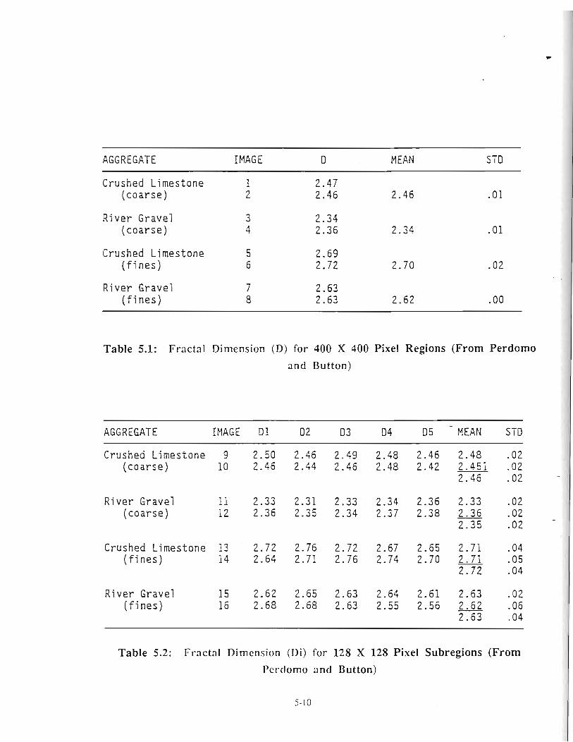
AGGREGATE IMAGE D MEAN STD

Crushed Limestone (coarse)

River Gravel (coarse)

Crushed Limestone ( f ines)

River Gravel ( f ines )

Table 5.1: Fractal Dimension (D) for 400 X 400 Pixel Regions (From Perdomo and Button)

- AGGREGATE IMAGE D l D 2 D3 D 4 D5 MEAN STD

Crushed Limestone 9 2.50 2.46 2.49 2.48 2.46 2.48 .02 (coarse) 10 2.46 2.44 2.46 2.48 2.42 2 .451 .02

2.46 .02

River Gravel 11 2.33 2.31 2.33 2.34 2.36 2.33 .02 (coarse) 12 2.36 2.35 2.34 2.37 2.38 2.36 .02

2.35 -

.02

Crushed Limestone 13 2.72 2.76 2.72 2 - 6 7 2.65 2 - 7 1 .04 ( f ines ) 14 2.64 2.71 2.76 2.74 2.70 2 . 7 1 .05

2.72 .04

River Gravel 15 2.62 2.65 2.63 2.64 2.61 2.63 .02 ( f ines) 16 2.68 2.68 2.63 2.55 2.56 2 .62 .06

2.63 .04

Table 5.2: FI-actal Dimcnsion (Di) for 128 X 128 Pixel Subregions (From

Pcr(lomo and Button)

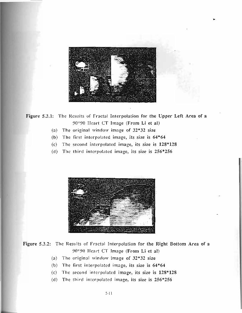
Figure 5.3.1: he Results of FI-actal Interpolation for the Upper Left Area of a 90*90 I.Icar-t CT Image (From Li et al)

(a) The original window image of 32*32 size

(b) The first interpolated image, its size is 64*64 (c) The seconcl interpolated image, its size is 128*128 (d) The third interpolated image, its size is 256*256

Figure 5.3.2: The Results of Fractal Interpolation for the Right Bottom Area of a

90*90 I-leal-t CT Image (From Li et al)

(a) The original window image of 32*32 size

(b) The first interpolated image, its size is 64*64

(c) Tile second interpolatecl image, its size is 128*128 (d) T h e third interpolatccl image, its size is 256*256

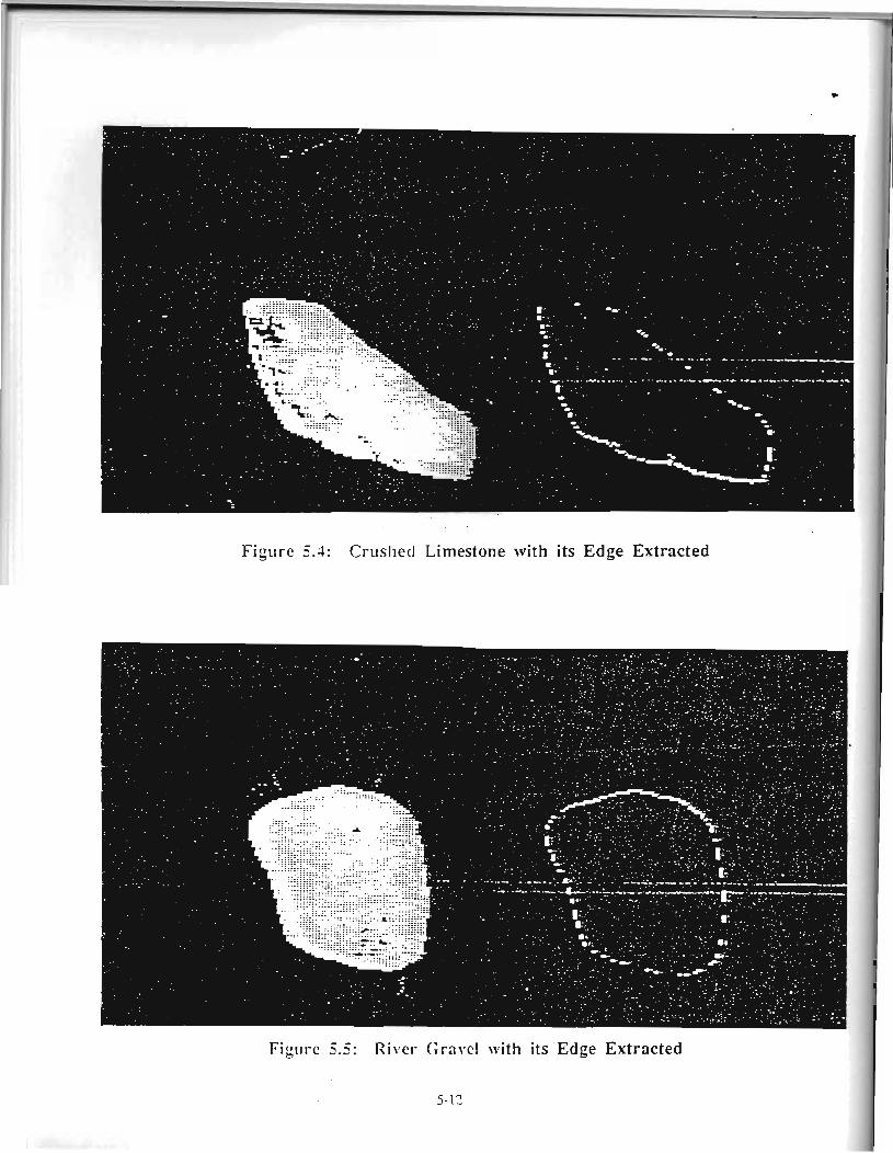
Figure 5.4: Crusllecl Limestone with its Edge Extracted

F i e 5 . 5 River Gravel with its Edge Extracted

5-12

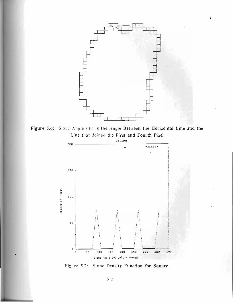
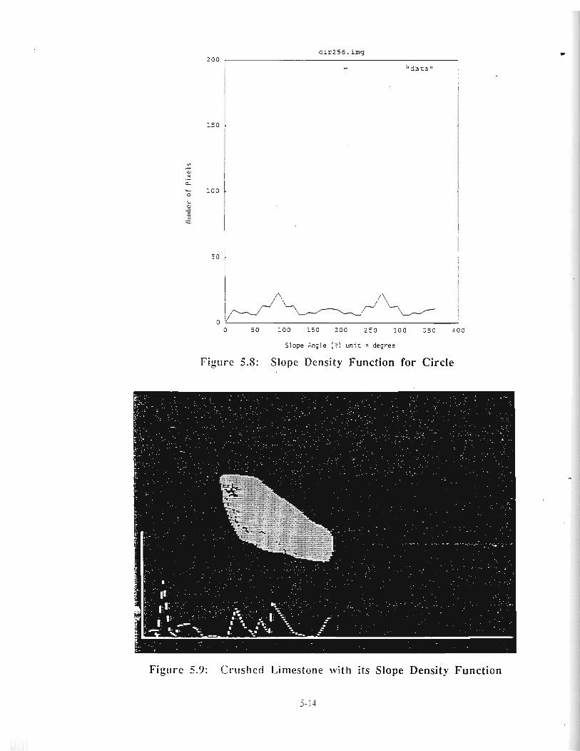
Slope Angle ( Y ) u n i t = degree

Figr~re 5.8: Slope Density Function for Circle

Figure 5.9: Crushctl Limestone with its Slope Density Function

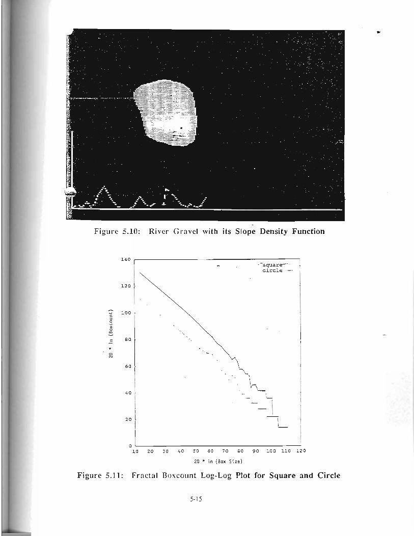
a l 3 ~ ! 3 pue a ~ e n b s JOJ $old 307-Sol lullonsou ICl3CJd : I 1-,c a ~ n 9 ! ~

021 015 OOT 06 00 OL 09 05 OP 01: OZ OX

I I I

D - - - OOT C

0 ZT

OPT

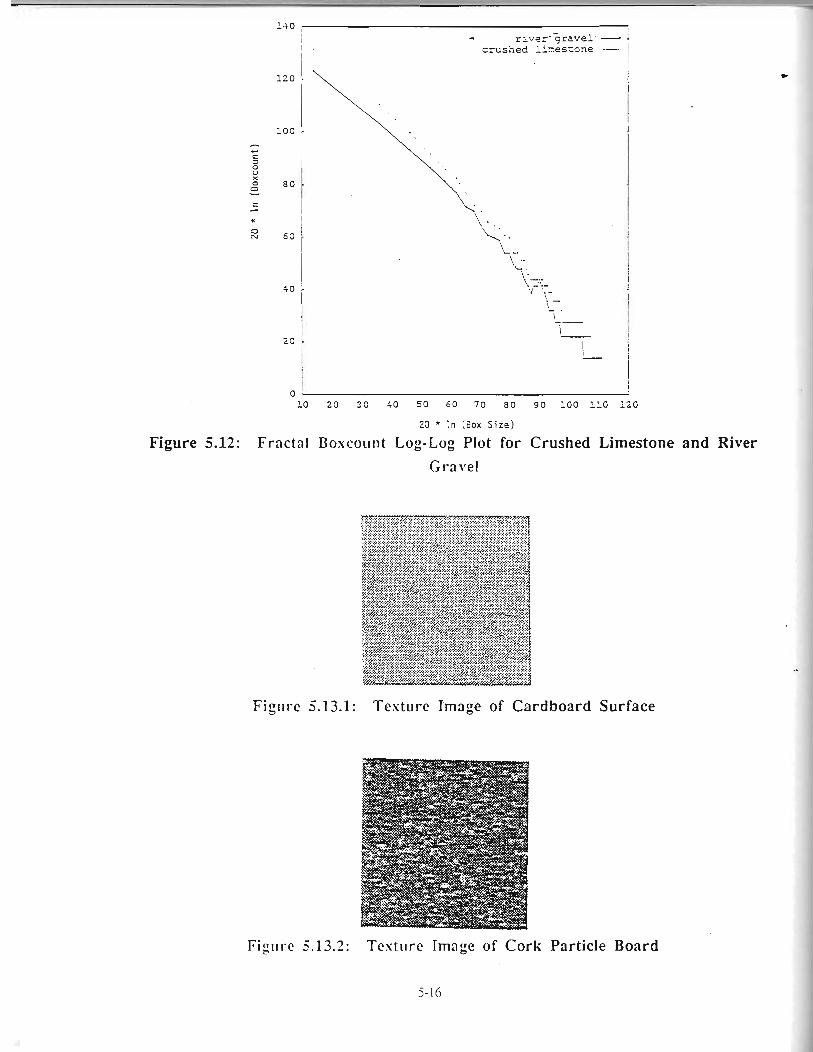
~ -- - river'^gravel. - i crushed lixesrsne -- I

I

20 * in (60x S i z e )

Figure 5.12: Fractal Boxcount Log-Log Plot for Crushed Limestone and River Gravel

Figr~r-e 5.13.1: Testure T'mage of Cardboard Surface

Figr~r-c 5.13.2: Tcsturc Image of Cork Particle Board

5- I6

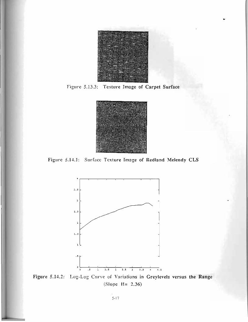
C't P 5 - c t 5.2 Z 5'1 T s- 0

1 O

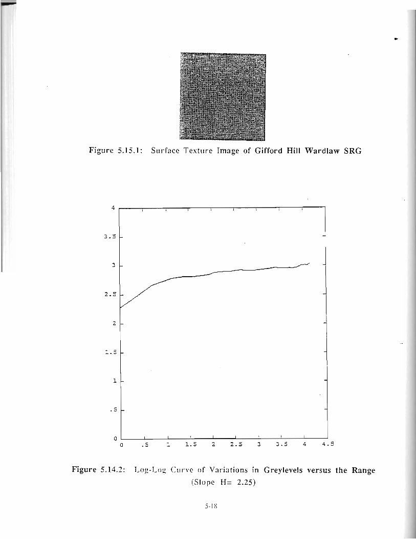
Figure 5.15.1: Sr~rfticc T e s t ~ ~ r e Image of Gifford Hill Wardlaw SRG

Figure 5.14.2: T,og-l,og Cirr-vc o f Vnr-iations in Greylevels versus the Range (Slopc I-[= 2.25)

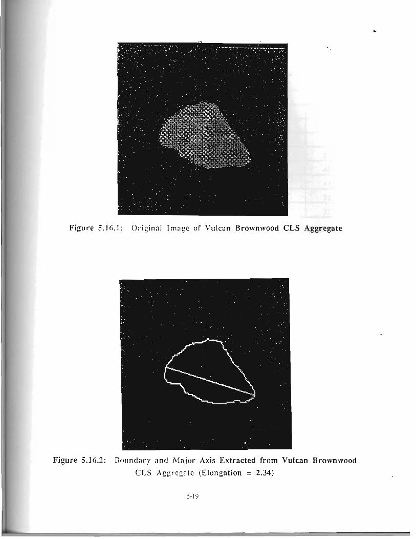
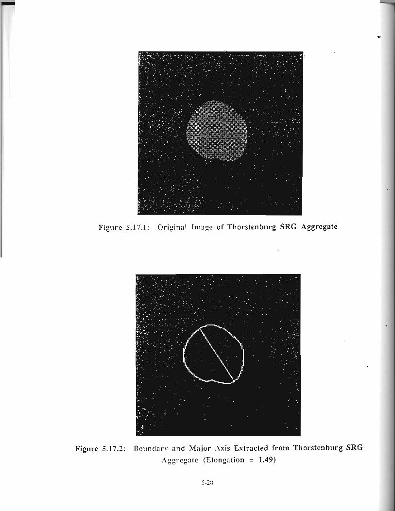
I I Figure 5.17.1: Original Image of Thorstenburg SRG Aggregate

Figure 5.17.2: Bountlar-y and Ma f or Axis Extracted from Thorstenburg SRG Aggrcgatc (Elongation = 1.49)

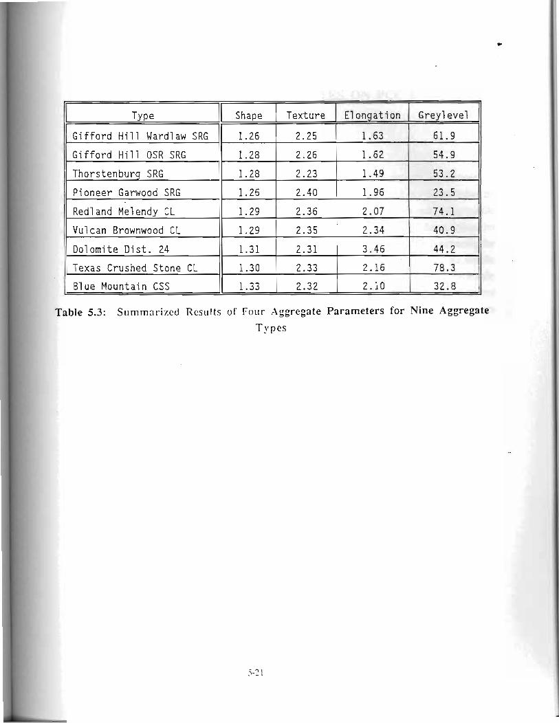
1

-

I I

Table 5.3: Summnl-izctf Rcsults of Four Aggregate Parameters for Nine Aggregate

Types

5-1- 1

i a --- - - - - - -

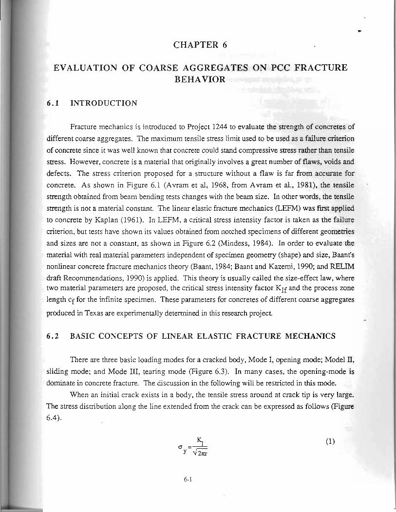
CHAPTER 6

EVALUATION OF COARSE AGGREGATES ON PCC FRACTURE BEHAVIOR

6 . 1 INTRODUCTION

Fracture mechanics is introduced to Project 1244 to evaluate the strength of concretes of

different coarse aggregates. The maximum tensile stress limit used to be used as a failure criterion

of concrete since it was well known that concrete could stand compressive stress rather than tensile

stress. However, concrete is a material that originally involves a great number of flaws, voids and

defects. The stress criterion proposed for a structure without a flaw is far from accurate for

1 concrete. As shown in Figure 6.1 (Avram et al, 1968, from Avram et al., 1981), the tensile .

strength obtained from beam bending tests changes with the beam size. In other words, the tensile

strength is not a material constant. The linear elastic fracture mechanics (LEFM) was first applied

to concrete by Kaplan (1961). In LEFM, a critical stress intensity factor is taken as the failure

criterion, but tests have shown its values obtained from notched specimens of different geometries

and sizes are not a constant, as shown in Figure 6.2 (Mindess, 1984). In order to evaluate the

material with real material parameters independent of specimen geometry (shape) and size, Baant's

nonlinear concrete fracture mechanics theory (Baant, 1984; Baant and Kazemi, 1990; and RELIM draft Recommendations, 1990) is applied. This theory is usually called the size-effect law, where two material parameters are proposed, the critical stress intensity factor KIf and the process zone

length cf for the infinite specimen. These parameters for concretes of different coarse aggregates

produced in Texas are experimentally determined in this research project

6 . 2 BASIC CONCEPTS OF LINEAR ELASTIC FRACTURE MECHANICS

There are three basic loading modes for a cracked body, Mode I, opening mode; Model 11,

sliding mode; and Mode 111, tearing mode (Figure 6.3). In many cases, the opening-mode is dominate in concrete fracture. The discussion in the following will be restricted in this mode.

When an initial crack exists in a body, the tensile stress around at crack tip is very large.

The stress distribution along the line extended from the crack can be expressed as follows (Figure

6.4).

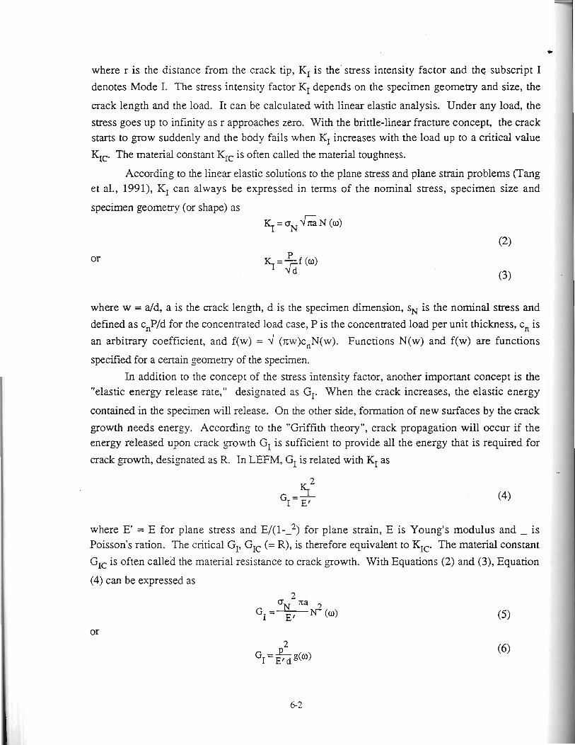
where r is the distance from the crack tip, KI is the stress intensity factor and the subscript I denotes Mode I. The stress intensity factor KI depends on the specimen geometry and size, the

crack length and the load. It can be calculated with linear elastic analysis. Under any load, the

stress goes up to infinity as r approaches zero. With the brittle-linear fracture concept, the crack starts to grow suddenly and the body fails when KI increases with the load up to a critical value

KIc. The material constant KIc is often called the material toughness.

According to the linear elastic solutions to the plane stress and plane strain problems (Tang et al., 1991), KI can always be expressed in terms of the nominal stress, specimen size and

specimen geometry (or shape) as ~=~,J-,N(o)

where w = a/d, a is the crack length, d is the specimen dimension, sN is the nominal stress and

defined as c,P/d for the concentrated load case, P is the concentrated load per unit thickness, c, is

an arbitrary coefficient, and f(w) = 4 (rrw)c,N(w). Functions N(w) and f(w) are functions

specified for a certain geometry of the specimen.

In addition to the concept of the stress intensity factor, another important concept is the "elastic energy release rate," designated as GI. When the crack increases, the elastic energy

contained in the specimen will release. On the other side, formation of new surfaces by the crack

growth needs energy. According to the "Griffith theory", crack propagation will occur if the I I

energy released upon crack growth GI is sufficient to provide all the energy that is required for I

crack growth, designated as R. In LEFM, GI is related with KI as I

I

where E' = E for plane stress and ~ / ( 1 - - ~ ) for plane strain, E is Young's modulus and - is Poisson's ration. The critical GI, GIc (= R), is therefore equivalent to KIc. The material constant

GIc is often called the material resistance to crack growth. With Equations (2) and (3), Equation

(4) can be expressed as

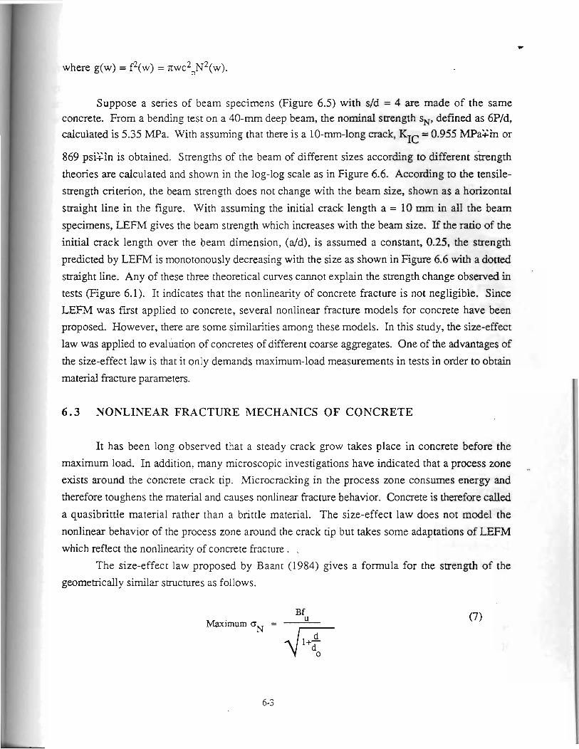
where g(w) = f2(w) = ~wc~ , . ,N~(w) .

Suppose a series of beam specimens (Figure 6.5) with s/d = 4 are made of the same concrete. From a bending test on a 40-mm deep beam, the nominal strength SN, defined as 6P/d, calculated is 5.35 MPa. With assuming that there is a 10-=-long crack, KIC = 0.955 MPaZm or

869 psijlin is obtained. Strengths of the beam of different sizes according to different sirength

theories are calculated and shown in the log-log scale as in Figure 6.6. According to the tensile-

strength criterion, the beam strength does not change with the beam size, shown as a horizontal

straight line in the figure. With assuming the initial crack length a = 10 mm in all the beam

specimens, LEFM gives the beam strength which increases with the beam size. If the ratio of the

initial crack length over the beam dimension, (dd), is assumed a constant, 0.25, the strength

predicted by LEFM is monotonously decreasing with the size as shown in Figure 6.6 with a dotted

straight line. Any of these three theoretical curves cannot explain the strength change observed in

tests (Figure 6.1). It indicates that the nonlinearity of concrete fracture is not negligible. Since

LEFM was first applied to concrete, several nonlinear fracture models for concrete have been

proposed. However, there are some similarities among these models. In this study, the size-effect

law was applied to evaluation of concretes of different coarse aggregates. One of the advantages of

the size-effect law is that it only demands maximum-load measurements in tests in order to obtain

material fracture parameters.

6 .3 NONLINEAR FRACTURE MECHANICS OF CONCRETE

It has been long observed that a steady crack grow takes place in concrete before the

maximum load. In addition, many microscopic investigations have indicated that a process zone

exists around the concrete crack tip. Microcracking in the process zone consumes energy and

therefore toughens the material and causes nonlinear fracture behavior. Concrete is therefore called

a quasibrittle material rather than a brittle material. The size-effect law does not model the

nonlinear behavior of the process zone around the crack tip but takes some adaptations of LEFM which reflect the nonlinearity of concrete fracture. ,

The size-effect law proposed by Baant (1984) gives a formula for the strength of the

geometrically similar structures as follows.

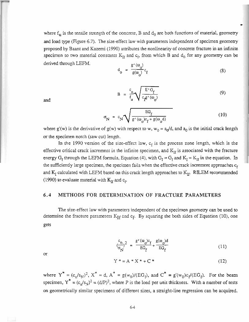
where f,, is the tensile strength of the concrete, B and do are both functions of material, geometry

and load type (Figure 6.7). The size-effect law with parameters independent of specimen geometry

proposed by Baant and Kazemi (1990) attributes the nonlinearity of concrete fracture in an infinite specimen to two material constants KIf and cf, from which B and for any geometry can be

derived through LEFM. g' (ao) - - -

*o g(oo) Cf

and

where g'(w) is the derivative of g(w) with respect to w, wo = add, and a. is the initial crack length

or the specimen notch (saw cut) length. In the 1990 version of the size-effect law, cf is the process zone length, which is the

effective critical crack increment in the infinite specimen, and KIf is associated with the fracture

energy Gf through the LEFM formula, Equation (4), with GI = Gf and KI = KIf in the equation. In

the sufficiently large specimen, the specimen fails when the effective crack increment approaches cf

and KI calculated with LEFM based on this crack length approaches to Kw RILEM recommended

(1990) to evaluate material with KIf and cf.

6.4 METHODS FOR DETERMINATION OF FRACTURE PARAMETERS

The size-effect law with parameters independent of the specimen geometry can be used to determine the fracture parameters KIf and cf By squaring the both sides of Equation (lo), one

gets

* where Y* = ( c ~ / s ~ ) ~ , X* = d, A = g(wO)/(EGf), and C* = g'(wo)cf/(EGf). For the beam

* specimen, Y = (cn/sN12 = (d/P12, where P is the load per unit thickness. With a number of tests

on geometrically similar specimens of different sizes, a straight-line regression can be acquired.

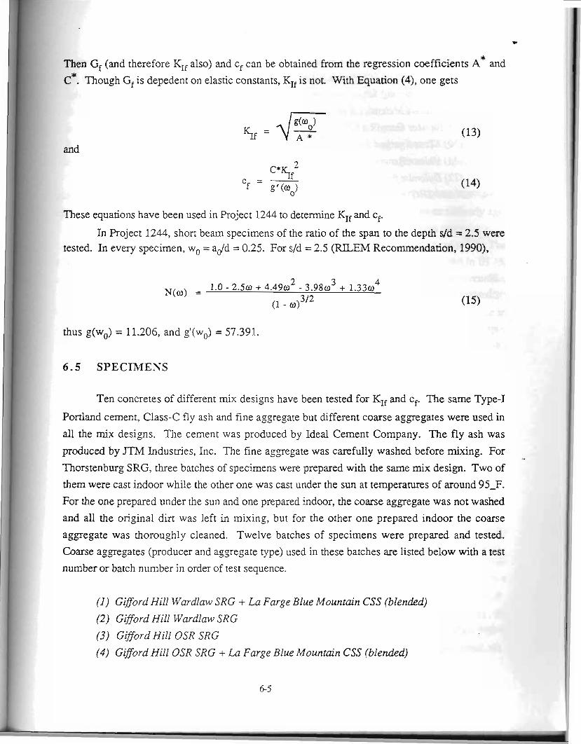
Then Gf (and therefore KIf also) and cf can be obtained from the regression coefficients A* and

c*. Though Gf is depedent on elastic constants, KIf is nor With Equation (4), one gets

and

I These equations have been used in Project 1244 to determine KIf and cf.

In Project 1244, short beam specimens of the ratio of the span to the depth s/d = 2.5 were tested. In every specimen, wo = add = 0.25. For s/d = 2.5 (RILEM Recommendation, 1990),

thus g(w,) = 11.206, and g1(wo) = 57.391.

6.5 SPECIMENS

Ten concretes of different mix desisns have been tested for KIf and cf. The same Type-I

Portland cement, Class-C fly ash and fine asgregate but different coarse aggregates were used in

all the mix designs. The cement was produced by Ideal Cement Company. The fly ash was I

produced by JTM Industries, Inc. The fine aggregate was carefully washed before mixing. For

Thorstenburg SRG, three batches of specimens were prepared with the same mix design. Two of

them were cast indoor while the other one was cast under the sun at temperatures of around 95-F. 1

I

i For the one prepared under the sun and one prepared indoor, the coarse aggregate was not washed

and all the original dirt was left in mixing, but for the other one prepared indoor the coarse 1

aggregate was thoroughly cleaned. Twelve batches of specimens were prepared and tested.

Coarse aggregates (producer and aggregate type) used in these batches are listed below with a test

number or batch number in order of test sequence.

( I ) Giford Hill Wardlaw SRG + La Farge Blue Mountain CSS (blended) 11

(2) Gifford Hill FVardlaw SRG

(3) Gifford Hill OSR SRG

(4) Gifford Hill OSR SRG + La Farge Blue Mountain CSS (blended)

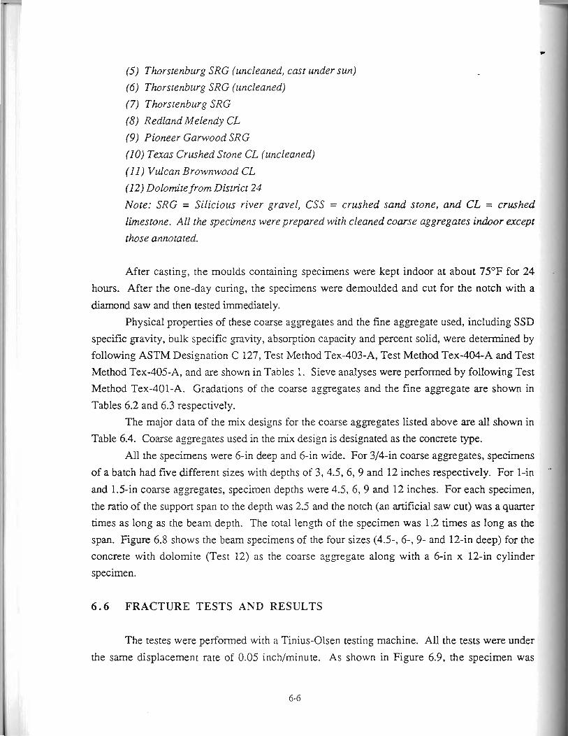
(5) Thorstenburg SRG (uncleaned, cast under sun)

(6) Thorstenburg SRG (~incleaned)

(7) Thorstenburg SRG

(8) Redland Melendy CL

(9) Pioneer Garwood SRG

(10) Texas Crushed Stone CL (~incleaned)

(11) Vulcan Brownwood CL

(12) Dolomite from District 24

Note: SRG = Silicious river gravel, CSS = crushed sand stone, and CL = crushed

limestone. All the specimens were prepared with cleaned coarse aggregates indoor except

those annotated.

After casting, the moulds containing specimens were kept indoor at about 75°F for 24

hours. After the one-day curing, the specimens were demoulded and cut for the notch with a

diamond saw and then tested immediately.

Physical properties of these coarse aggregates and the fine aggregate used, including SSD specific gravity, bulk specific gravity, absorption capacity and percent solid, were determined by

following ASTM Designation C 127, Test Method Tex-403-A, Test Method Tex-404-A and Test

Method Tex-405-A, and are shown in Tables 1. Sieve analyses were performed by following Test

Method Tex-401-A. Gradations of the coarse aggregates and the fine aggregate are shown in

Tables 6.2 and 6.3 respectively. The major data of the mix designs for the coarse aggregates listed above are all shown in

Table 6.4. Coarse aggregates used in the mix design is designated as the concrete type.

All the specimens were 6-in deep and 6-in wide. For 314-in coarse aggregates, specimens

of a batch had five different sizes with depths of 3,4.5, 6, 9 and 12 inches respectively. For 1-in "

and 1.5-in coarse aggregates, specimen depths were 4.5,6,9 and 12 inches. For each specimen,

the ratio of the support span to the depth was 2.5 and the notch (an artificial saw cut) was a quarter

times as long as the beam depth. The total length of the specimen was 1.2 times as long as the

span. Figure 6.8 shows the beam specimens of the four sizes (4.5, 6-, 9- and 12-in deep) for the concrete with dolomite (Test 12) as the coarse aggregate along with a 6-in x 12-in cylinder

specimen.

6 .6 FRACTURE TESTS AND RESULTS

The testes were performed with a Tinius-Olsen testing machine. All the tests were under

the same displacement rate of 0.05 inch/minute. As shown in Figure 6.9, the specimen was

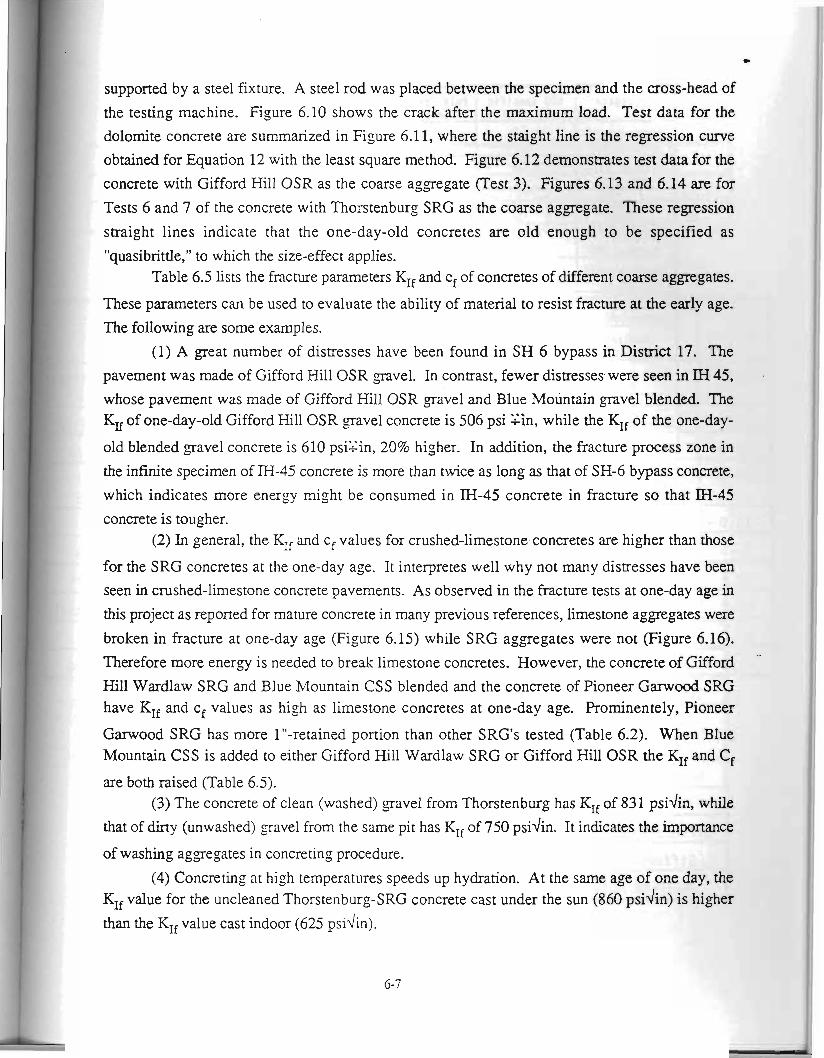
supported by a steel fixture. A steel rod was placed between the specimen and the cross-head of

the testing machine. Figure 6.10 shows the crack after the maximum load. Test data for the

dolomite concrete are summarized in Figure 6.1 1, where the staight line is the regression curve

obtained for Equation 12 with the least square method. Figure 6.12 demonstrates test data for the

concrete with Gifford Hill OSR as the coarse aggregate (Test 3). Figures 6.13 and 6.14 are for

Tests 6 and 7 of the concrete with Thorstenburg SRG as the coarse aggregate. These regression

straight lines indicate that the one-day-old concretes are old enough to be specified as

"quasibrittle," to which the size-effect applies. Table 6.5 lists the fracture parameters KIf and cf of concretes of different coarse aggregates.

These parameters can be used to evaluate the ability of material to resist fracture at the early age.

The following are some examples.

(1) A great number of distresses have been found in SH 6 bypass in District 17. The

pavement was made of Gifford Hill OSR gavel. In contrast, fewer distresses. were seen in M 45,

whose pavement was made of Gifford Hill OSR ,gravel and Blue Mountain gravel blended. The KU of one-day-old Gifford Hill OSR gravel concrete is 506 psi Ein, while the KIf of the one-day-

old blended gravel concrete is 610 psigin, 20% higher. In addition, the fracture process zone in

the infinite specimen of IH-45 concrete is more than twice as long as that of SH-6 bypass concrete,

which indicates more energy might be consumed in IH-45 concrete in fracture so that M-45

concrete is tougher. (2) In general, the KIf and cf values for crushed-limestone concretes are higher than those

for the SRG concretes at the one-day age. It interpretes well why not many distresses have been

seen in crushed-limestone concrete pavements. As observed in the fracture tests at one-day age in

this project as reported for mature concrete in many previous references, limestone aggregates were

broken in fracture at one-day age (Figure 6.15) while SRG aggregates were not (Figure 6.16).

Therefore more energy is needed to break limestone concretes. However, the concrete of Gifford "

Hill Wardlaw SRG and Blue Mountain CSS blended and the concrete of Pioneer Garwood SRG have KIf and cf values as high as limestone concretes at one-day age. Prominentely, Pioneer

Garwood SRG has more 1"-retained portion than other SRG's tested (TabIe 6.2). When Blue Mountain CSS is added to either Gifford Hill Wardlaw SRG or Gifford Hill OSR the KIf and Cf

are both raised (Table 6.5). (3) The concrete of clean (washed) gravel from Thorstenburg has KIf of 831 psidin, while

that of dirty (unwashed) gravel from the same pit has KIf of 750 psidin. It indicates the importance

of washing aggregates in concreting procedure.

(4) Concreting at high temperatures speeds up hydration. At the same age of one day, the KIf value for the uncleaned Thorstenburg-SRG concrete cast under the sun (860 psidin) is higher

than the KIf value cast indoor (625 psidin).

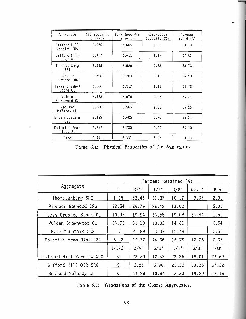
Table 6.1: Physical Properties of the Aggregates.

Aggregate

Gifford Hill Ward1 aw SRG

Gifford Hill OSR SRG

Thorstenburg SRG

Pioneer Garwood SRG

Texas Crushed Stone CL

Vul can Brownwood CL

Red1 and Me1 endy C L

Bl ue Mountain css

Do1 omi t e from Dis t . 24

Sand

Table 6.2: Gradations of the Coarse Aggregates.

SSD Specific Gravity

2.646

2.467

2.588

2.796

2.566

2.688

2.600

2.499

2.757

Aggregate

Thor s t enburg SRG

P ionee r Garwood SRG

Texas Crushed S t o n e CL

Vulcan Brownwood C L

Blue Mountain CSS

Dolomite from Dist. 24

G i f f o r d Hi1 1 Ward1 aw SRG

G i f f o r d H i l l OSR SRG

Redland Melendy C L

Bul k Speci f ic Gravity

2.604

2.411

2.580

,2.783

2.517

2.676

2.566

2.405

2.730

Percen t Reta ined (X)

2.441 1 2.331

1"

1.26

28.54

10.95

33.72

0

6.42

1-1/2"

0

0

0

Absorption Capacity (%)

1.59

Percent Sol id (%)

60.70

5.31

3/4"

52.46

26.79

19.94

'33.i0

21.89

19.77

3/4"

23.50

2.86

44.28

j 69.13 1

, 2.27 1 57.81 1

1/2"

23.87

25.42

23.58'

18.03

63.07

44.66

5/8"

12.45

6.96

10.94

0.33

0.46

1.91

0.46

1.31

3.76

0.99

58.73

54.28

55.78

53-21 I 56.25 1

!

55.31

54.10

I

3/8"

10.17

13.03

19.08

14.61

12.49

16.75

1/2"

23.35

, 22.32

13.33

No. 4

9.33

24.94

12.06

3/8"

18.01

30.35

19.29

Pan

2.91

5.01

1.51

0.54

2.55

0.35

Pan

22.69

37.52

12.15

-

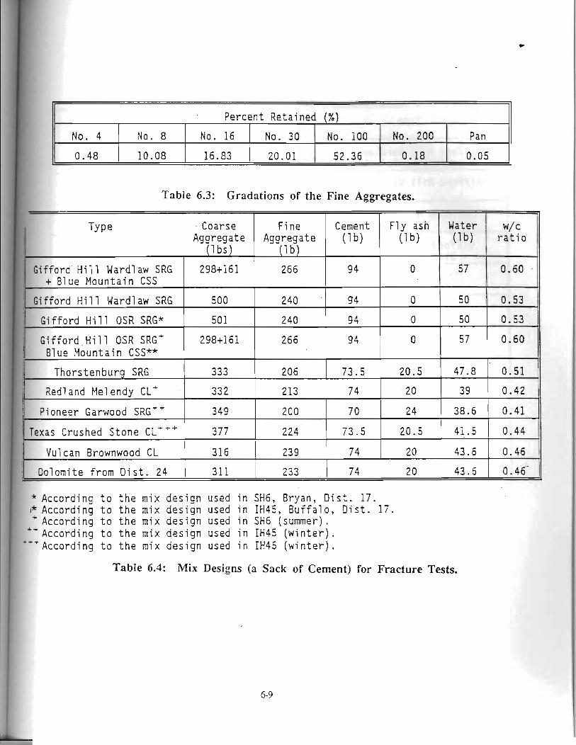
Percent Retained (%)

C

w

--- -

I Table 6.3: Gradations of the Fine Aggregates.

I

Water ( l b )

5 7

50

50

57

47.8

3 9

38.6

Fly ash (1 b)

0

0

0

0

20.5

20

24

20.5

20

2 0

Pan

0.05

I

w/c r a t i o

0.60 .

0.53

0.53

0.60

0.51

0.42

0.41

No. 4

0.48

* According t o t h e mix des ign used in SH6, Bryan, Dist. 17. I* According t o t h e mix des ign used in IH45, Buf fa lo , D i s t . 17.

I i

'According t o t h e mix des ign used in SH6 (summer). I i .b According t o t h e mix des ign used in IH45 ( w i n t e r ) .

'"According t o t h e mix des ign used in IH45 ( w i n t e r ) .

Table 6.4: Mix Designs (a Sack of Cement) for Fracture Tests.

6-9

-.- --- -- - -.- . .

Fine Aggregate

(1 b)

266

240

240

266

206

213

200

Coarse Aggregate

(1 bs)

298+161

500

50 1

298+161

333

332

349

377

I

I I

I

No. 16

16.83

No. 8

10.08

Cement (1 b)

94

9 4

9 4

9 4

73.5

7 4

7 0

T Y P ~

Gifford Hi1 1 Ward1 aw SRG t Blue Mountain CSS

Gi f fo rd Hi 11 Ward1 aw SRG

Gifford Hi1 1 OSR SRG*

Gif fo rd .Hi l1 OSR SRG+ Blue Mountain CSSf*

Thors tenburg SRG

Redland Melendy CL+

i ,

41.5 1 0.44 224 1 73.5

1 Pioneer Garwood SRG"

1 Texas Crushed S t o n e CL+'+

43.6

43.6

0.46 1 0.46. 1

Vulcan Brownwood C L 316 1 239

No. 200

0.18

No. 30

20.01

7 4

No. 100

52.36

Dolomite from D i s t . 24 1 311 233 1 74

- - - - - -

*

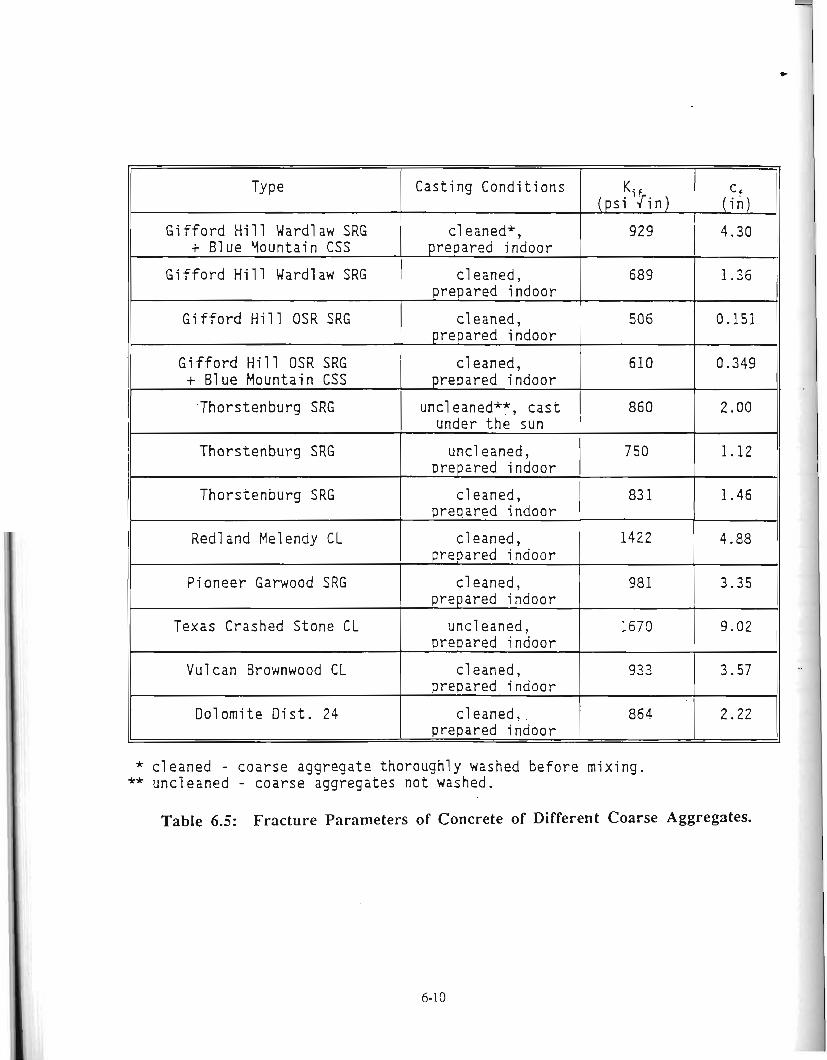
* c l e a n e d - c o a r s e agg rega te thoroughly washed b e f o r e mixing. ** uncleaned - c o a r s e aggrega tes not washed.

Table 6.5: Fracture Parameters of Concrete of Different Coarse Aggregates.

Type

Gi f f o r d H i 11 Ward1 aw SRG + Blue Mountain CSS

Gi f f o r d H i 11 Ward1 aw SRG

G i f f o r d Hill OSR SRG

G i f f o r d H i l l OSR SRG + Blue Mountain CSS

Thor s t enburg SRG .

Thors t enburg SRG

Thors t enburg SRG

Redland Melendy C L

P i o n e e r Garwood SRG

Texas Crashed Stone C L

Vulcan Brownwood C L

Do1 omi t e D i s t . 24

Cas t ing Cond i t i ons

c l eaned*, prepared indoor

c l eaned, prepared indoor

c1 eaned, prepared indoor

cl eaned, prepared indoor

uncl caned**, c a s t under the sun

uncl eaned, prepared indoor

c l e a n e d , prepared indoor

cl eaned, prepared indoor

c l eaned , prepared indoor

uncl eaned , p r e ~ a r e d indoor

c1 eaned , prepared indoor

c l eaned, prepared indoor

'if ( p s i J i n )

929

689

506

610

860

750

83 1

1422

98 1

1670

933

864

= f ( i n )

4.30

1.36

0.151

0.349

2.00

1.12

1.46

4.88 1 3.35

9.02

3.57

2.22 1

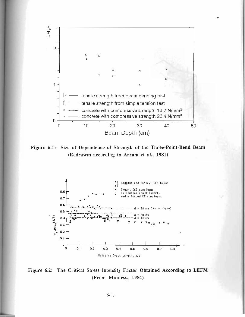
Beam Depth (cm)

- -

- -

-

-

- -

-

-

-

-

Figure 6.1: Size of Dependence of Strength of the Three-Point-Bend Beam (Redrawm according to Arram et al., 1981)

,>

0 0 a 0 0

0

0

fb - tensile strength from beam bending test

ft - tensile strength from simple tension test 0- concrete with compressive strength 13.7 N/mm2 o - concrete with compressive strength 26.4 N/mm2

I I I I I I I I I

t 8} l l iggins and Bai ley, SEN beams A

+ Brown. DCB specimens + + + + v l l i l l emeier and I l i l s d o r f .

wedge loaded CT specimens 0.7

Rela t ive crack' Length, a/b

Figure 6.2: The Critical Stress Intensity Factor Obtained According to LEFM (From Mindess, 1984)

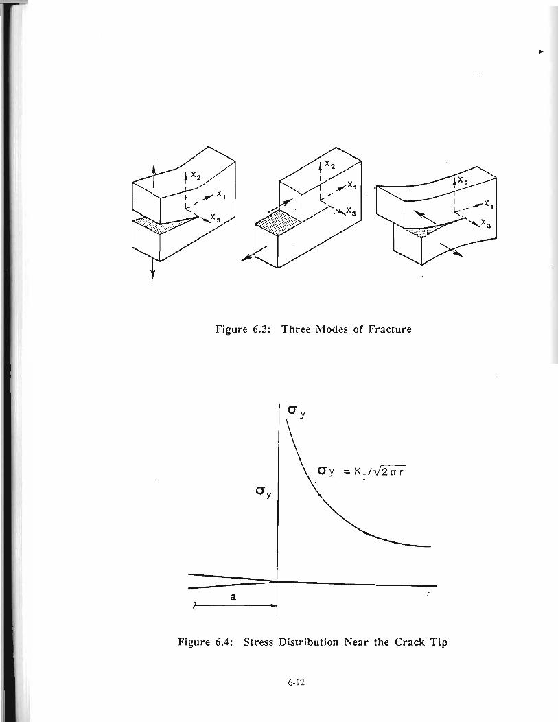
Figure 6.3: Three Modes of Fracture

I

Figure 6.4: Stress Distribution Near the Crack Tip

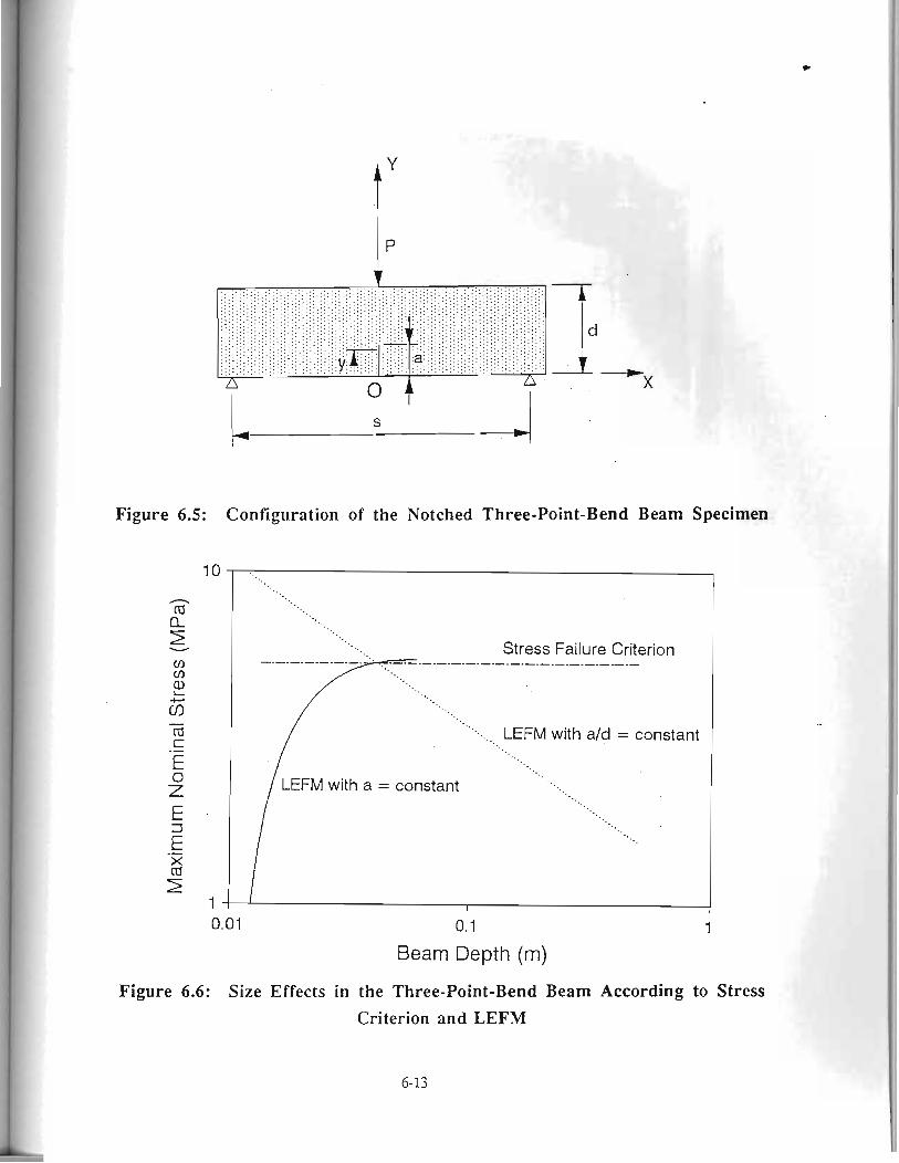
Figure 6.5: Configuration of the Notched Three-Point-Bend Beam Specimen

Figure 6.6: Size Effects in the Three-Point-Bend Beam According to Stress Criterion and LEFM

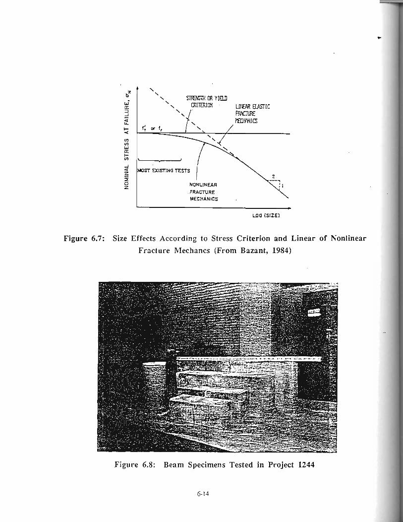
4 \ \ \ \

srarmc OR Ylrn \ Cfu'lERIcft . UIUlREIPSTIC

FRNN7E

K)ZT MlSTING TEZTS

FRACTURE MECHANICS -

Figure 6.7: Size Effects According to Stress Criterion and Linear of Nonlinear Fracture Mechancs (From Bazant, 1984)

Figure 6.8: Beam Specimens Tested in Project 1244

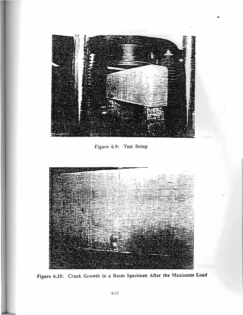
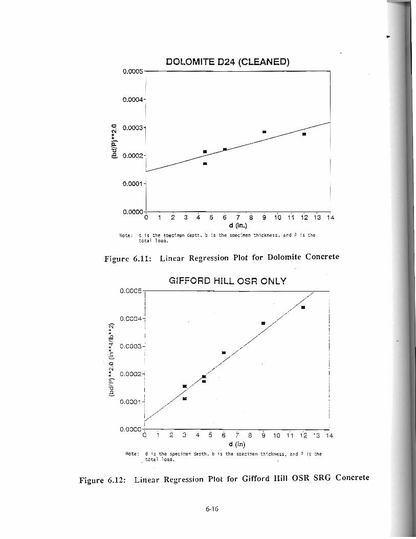
DOLOMITE D24 (CLEANED) 0.0005 1

o.ooo0 o / i i 3 i s 5 7 8 9 i o i 1 1 i l i 1 I

d (in-) Note: d is the soecimen depth, b is the specimen thickness, and ? is the

total load.

Figure 6.11: Linear Regression Plot for Dolomite Concrete

GlFFORD HILL OSR ONLY

d (in) Note: d is the saecimen deoth, b is the specimen thickness, and P i s the

total load.

Figure 6.12: Linear Regression Plot for Gifford Hill OSR SRG Concrete

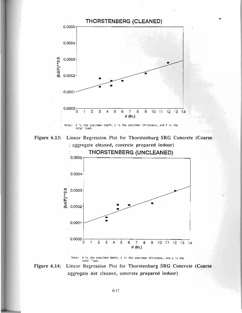
THORSTENBERG (CLEANED) 0.0005-

0.0004-

, Note: d is the soecimen depth, b is the specimen thickness, and ? is the total load.

Figure 6.13: Linear Regression Plot for Thorstenburg SRG Concrete (Coarse aggregate cleaned, concrete prepared indoor)

THORSTENBERG (UNCLEANED)

0.0000 ! o i 2 3 4 5 6 i i 9 1 0 1 i 1 2 1 3 i k d (In.)

Note: d is the soecimen depth, b is the saecimen thickness, and p is the total load.

Figure 6.14: Lincnr Regression Plot for Thorstenburg SRG Concrete (Coarse

aggregate not cleaned, concrete prepared indoor)

6-17

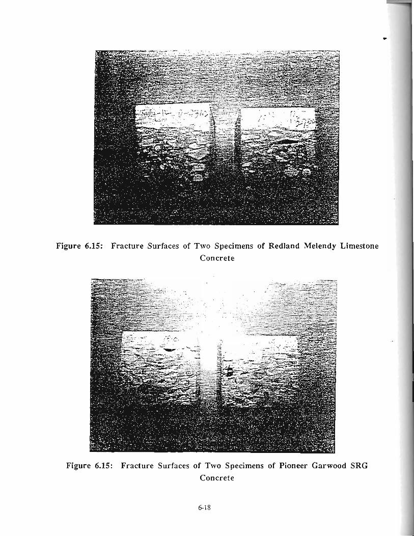
Figure 6.15: Fracture Surfaces of Two Specimens of Redland Melendy Limestone Concrete

Figure 6.15: Fracture Surfaces of Two Specimens of Pioneer Garwood SRG

Concrete

6.7 REFERENCE

1. Avram, C., F\c\oaru, I., Filimon I., M4rYu, O., and Tertea, I., (1981), Concrete Stren~th and Strains, Elsevier, New York.

2. Ba-ant, 2. P., (1984), "Size Effect in Blunt Fracture: Concrete, Rock, Metal," Journal of Engineerine Mechanics, Vol. 110, No. 4.

3. Ba-ant, 2. P., and Kazemi, M. T., (1990), "Determination of Fracture Energy, Process Zone Length and Brittleness Number from Size Effect, with Application to Rock and Concrete," International Journal of Fracture, Vol. 44.

4. Kaplan, M. F., (1961), "Crack Propagation and the Fracture of Concrete," Journal of thc American concrete Institute, Vol. 58, No. 5.

5. Mindess, S., (1984), "Fracture Toughness Testing of Cement and Concrete," Fracture Mechanics of Concrete, eds. Carpinteri, A. and Ingraffea, A. R., Martinus Nijhoff Publishers.

6. RILEM Draft Recommendations (1990), "Size-Effect Method of Determining Fracture Energy and Process Zone Size of Concrete," Materials and Structures, RILEM, Vol. 23, No. 138.

7. Tang, T., Shah, S. P., and Ouyang, C., (1991), "Fracture Mechanics and Size Effect of Concrete in Tension," submitted to ASCE Journal of Structure Engineering.

CHAPTER 7

DETERMINATION OF SAW-CUT DEPTH AND SPACING WITH FRACTURE ANALYSIS

7.1 INTRODUCTION

In newly paved concrete pavements, the temperature rise caused by the hydration process

can be considerable. If u~estrained, the concrete pavement can expand and contract during the

heating and subsequent cooling process without stresses being induced. Similar displacements

may result due to shrinkage as the pavement dries and expand when it is wetted. However, actual

pavements in the field, are nearly always restrained to some degree either by external restraint such

as friction, the slab weight, tied adjoining lanes, or a combination of these. Interaction of the .

induced temperature and drying shrinkage gradients and the slab restraint can induce tensile -

stresses, that lead to slab cracking.

Field experiments have indicated that typically many sawcut joints break in the concrete

pavement within the first few days after placement under hot weather concreting conditions. It is

evident that an understanding of the mechanism related to early-age cracking in concrete pavements

should provide a basis for improvements in current pavement sawcutting practice with respect to an

appropriate combination of sawcut timing and sawcut depths. The sawcut should be deep enough

such that a crack initiated at a sawcut-surface notch will propagate in an unstable manner from the

sawcut tip to the slab bottom under stresses caused by temperature and shrinkage gradients or

variations. Since this cracking consumes elastic energy which developed within the concrete slab,

stress and the incidence of cracking elsewhere is reduced in the slab. The controlled cracks reduce

the restraint in the concrete pavement slab and therefore lowers the maximum tensile stress. One- -- third of the pavement thickness (d/3) has been accepted and assumed to be the necessary depth of

cut since the early 1950's. However, literature reviews reveal little technical justification for this

assumption, other than field experience in isolated instances of uncontrolled'cracking in which

engineers may have assumed that deeper sawcuts would solve the problems they were

experiencing with random cracking. It will be shown later that little benefit is to be gained from -

deeper sawcuts and that the most significant factor in the effective control of random cracking is the

time of sawcut placement. In this sense, a sawcut depth of d/3 or d/4 without respect to aggregate

type, concrete properties, or pavement thickness characteristics is technically unjustified. The

conventional analysis of crack development in sawcut concrete pavement typically assumes a flawless beam or plate, although crack formation and development is of primary interest. In this

paper, fracture mechanics is applied to determine sawcut depth requirements based on stresses

which develop during the first few days after placement. Since the use of fracture mechanics to

analyze sawcut depth criteria in jointed concrete systems constitutes a new approach to analyze

crack development (and basically the only rational approach to accurately account for the factors

pointed out above), sufficient mathematical derivation will be provided to adequately document and

justify the approach.

7.2 THEORETICAL APPROACH: CLIMATIC STRESSES

Environmental stresses in concrete pavements may be attributed to both temperature and

drying shrinkage affects and are particularly important at an early age. Stresses causes by both of

these effects are discussed subsequently.

7 .2 .1 Thermal Stresses The growth of early-age thermal stresses in a concrete structure, may be illustrated in the -

consideration of a fully-restrained concrete element in which the stress state is uniaxial (Figure 7.1) during a heating and cooling cycle. Laboratory tests [7.1] have indicated that during the first few

hours after placement while the concrete is fully plastic no measurable stress build-up occurs.

After this plastic stage, the strength of the concrete can increase rapidly where continued rise in

temperature induces compressive stresses. However, due to the high creep of early-aged concrete,

the compressive stresses may be substantially relaxed. In the referenced study, laboratory results

indicated that a temperature maximum occurred at about 26 hours after casting of concrete but

relaxation within the concrete occmed leading to a possible zero stress condition. (Due to varying

temperature conditions, this process may proceed at varying rates under field conditions.) As

cooling proceeds, tensile stresses gradually develop and increase until finally a tensile failure

occurs. Thus, tensile stresses and thermal cracking in the structure result from temperature and -- shrinkage affects during the early stages of hydration while the concrete is developing increasing

stiffness. Due to exposure to ambient conditions, a concrete pavement may cool to a minimum

temperature after cycling through a maximum temperature such that tensile stresses can be induced

in the slab. The tensile stress dismbution through the pavement thickness can be assumed to be .

linear for the sake of simplicity but others [7.2] have indicated that the dismbution may be

decomposed into three parts: axial stress, curling stress and nonlinear stress. Not only is the

stress dismbution caused by a temperature effect, as referenced above, but it may also be caused

by moisture effects which was not included in the above referenced study. Therefore, a complete

analysis of early-aged stresses will include curling, warping, and frictional stresses where the axial

stress component may be primarily due to subbase/subgrade frictional effects. Stress development

* may become significant very soon after placement perhaps even before the concrete has attained a

certain degree of stiffness (which may not occur until 18 to 24 hours after placement) has

developed. Crack development in concrete pavements has been noted to be sensitive to diural

temperature effects. The tendency to curl is restrained by the slab weight in which the resulting

level of stress development is a function of the stiffness of the subbase layer as reflected in the

radius of relative stiffness ( p ). When the slab curls in an upwards configuration, tensile stresses

are induced in the upper part of the slab while compressive stresses are induced in the lower part.

Analysis of stress induced by a linear temperature gradient in rigid pavements was developed by

Westergaard [7.3] and others [7.4]. The Westergaard solution for slab stresses under temperature gradients will not be

elaborated here. However, a similar approach will be presented later for slab stresses caused by

moisture gradients. Westergaard presented solutions which considered curling stresses in a slab of

infinite and semi-infinite dimensions based on the following governing equations:

~h where 1 - [ ] as pointed out previously is called the radius of relative stiffness and:

12 (1 -u2) k

E = Young's modulus (psi) v = Poisson's ratio

k = Foundation modulus (psihi)

h = Slab thickness (in)

w = Slab deflection (in).

Equation (1) encompasses a spring model that was proposed for the base reaction with the k value

as the spring modulus. Though the slab weight restrains the curling, the weight is not included in

the equation. However, the displacement (w) caused by curling can be considered only part of the slab displacement C7.51. In addition to w, the slab weight causes a uniform subsidence w,. The total displacement w, is the sum of w, and w. So long as w, = w, + w 2 0, the spring model is

valid even if w < 0. The solution to Equation (1) indicates a negative w or upward displacements at and near

the slab edge in concave curling, which should not be interpreted that the slab is pulled down there

by the base. Wherever w c 0, part of the slab weight is supported by the base while the rest of it is supported by the slab itself which contributes to the stresses in the slab. The total displacement w,

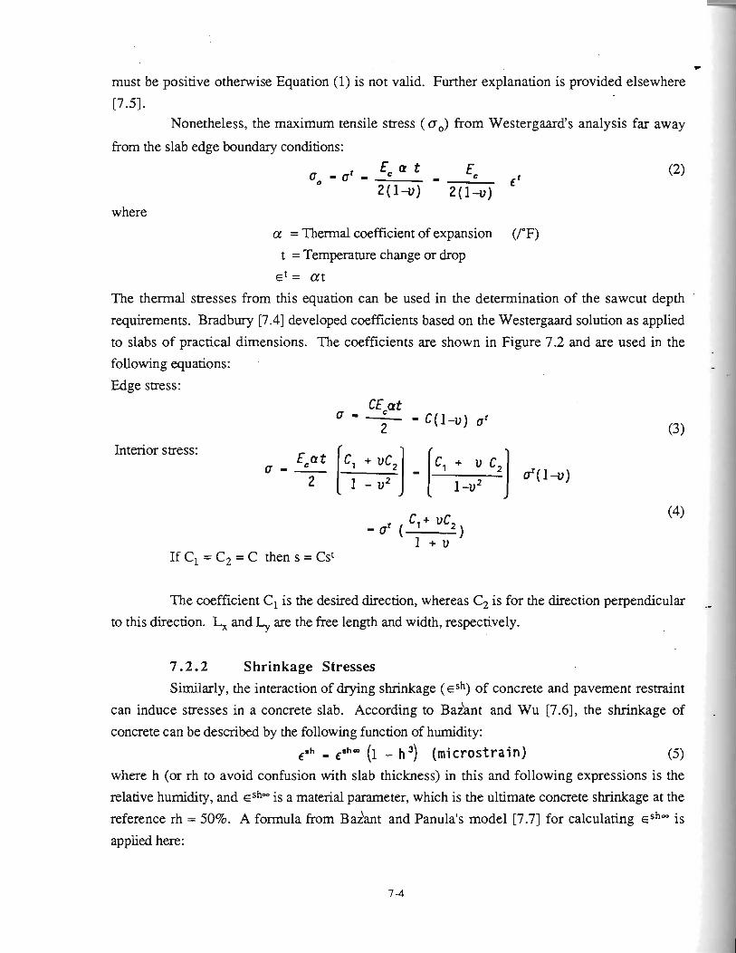
* must be positive otherwise Equation (1) is not valid. Further explanation is provided elsewhere

17.51. Nonetheless, the maximum tensile stress (a,) from Westergaard's analysis far away

from the slab edge boundary conditions:

where a = Thermal coefficient of expansion (/OF)

t = Temperature change or drop

E' = a t

The thermal stresses from this equation can be used in the determination of the sawcut depth

requirements. Bradbury [7.4] developed coefficients based on the Westergaard solution as applied

to slabs of practical dimensions. The coefficients are shown in Figure 7.2 and are used in the

following equations:

Edge stress:

Interior stress: + v Cz

2 a'(1 -v)

The coefficient C1 is the desired direction, whereas C2 is for the direction perpendicular .-

to this direction. L, and $ are the free length and width, respectively.

7.2.2 Shrinkage Stresses Similarly, the interaction of drying shrinkage ( E S ~ ) of concrete and pavement restraint

can induce stresses in a concrete slab. According to ada ant and Wu [7.6], the shrinkage of

concrete can be described by the following function of humidity: csh - Erh' (1 - h3) (microstrain) (5)

where h (or rh to avoid confusion with slab thickness) in this and following expressions is the

relative humidity, and E S ~ " is a material parameter, which is the ultimate concrete shrinkage at the

reference rh = 50%. A formula from ~az'ant and Panula's model [7.7] for calculating eshW is

applied here:

D- -113 S

1 + - z - 0.381 6 [1.25 [:rn + 0.5 [:]I w c - 12

(8)

- C

where a

ale Total aggregatelcement ratio

gIs= Coarse aggregatdfine aggregate ratio

SIC= Fine aggregatdcement ratio

W/C= Waterlcement rado

fa = 28-day cylinder compressive strength (psi)

In the infinitely large concrete slab, , the shrinkage is

totally restrained. The shrinkage-induced stresses ( ash) are:

Moisture measurements in actual field slabs, using instrumentation described by others

[7.8], have indicated that process tends to go through to the bottom of the concrete slab. These

measurements have also indicated the non-linearity of the humidity profile vertically through a

pavement slab during wetting and drying cycles. One would expect that such variations will result

in similar profiles or distributions of moisture-induced warping stresses. The representation of

these distributions numerically in analysis may well require sophisticated methods such as the finite

element or finite difference approaches. However, for the purpose of introducing an approach to

the analysis of moisture-induced warping analysis, the moisture-induced stress distribution in a

concrete slab is simplified (as was done for temperature-gradient related stresses) to vary linearly

along the thickness with the maximum tensile stress a s h at the top surface as shown in Figure 3.

If it is assumed that the shrinkage stress distributes linearly through the thickness of the slab,

varying from a s h at the top to zero at the bottom. The solutions provided by Westergaard [7.3]

and Bradbury [7.4] can be implemented by only replacing ~t in all the equations (e.g. equations

(2) to (4)) by esh. Another simplification results in no shrinkage related stresses within -H/2 < z < h/2 (0 < H < h - as defined in Figure 3) and that the shrinkage-induced normal stress ash linearly

decreases from z - -h/2 to 0 at z = -W2. Work is currently underway at the Texas Transportation

Institute to model and verify the non-linear temperature and moisture stress distributions in jointed

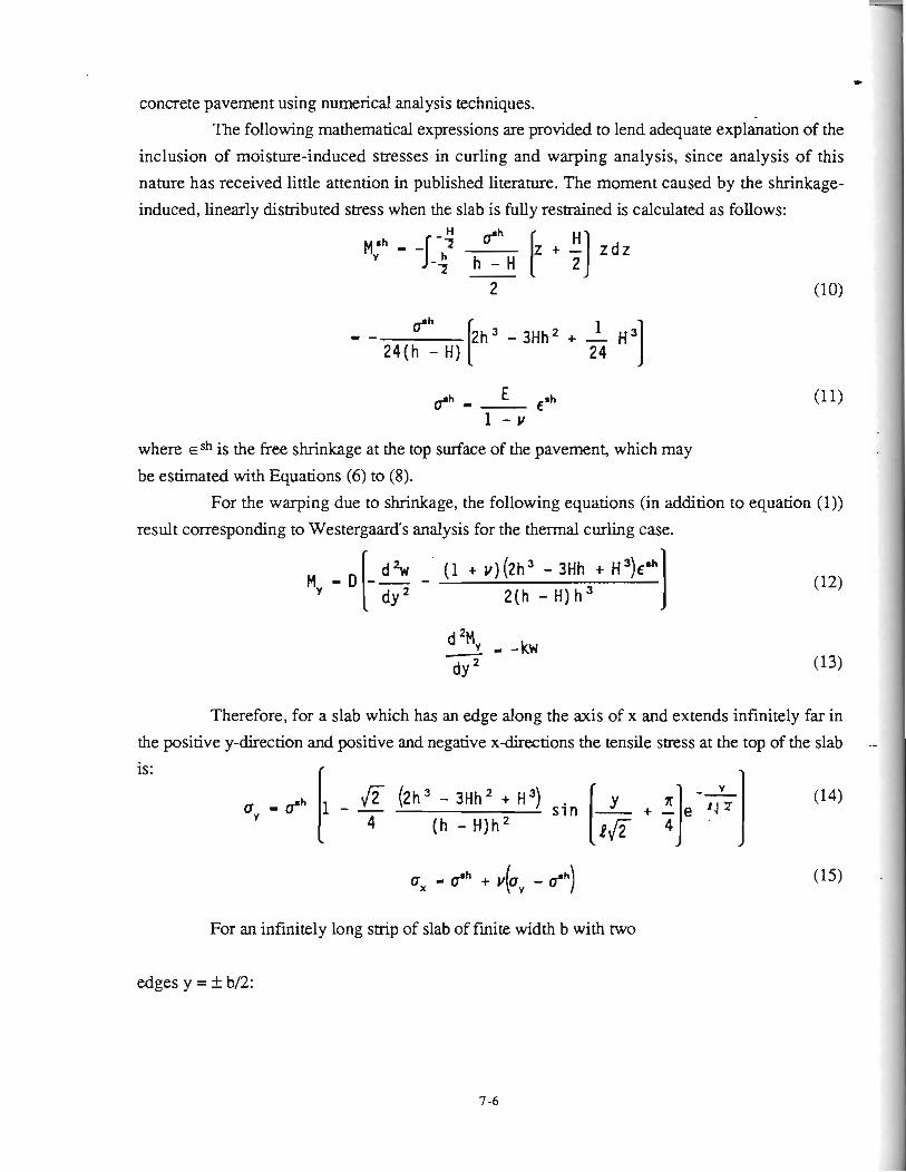
w

concrete pavement using numerical analysis techniques.

The following mathematical expressions are provided to lend adequate explanation of the

inclusion of moisture-induced stresses in curling and warping analysis, since analysis of this

nature has received little attention in published literature. The moment caused by the shrinkage-

induced, linearly distributed stress when the slab is fully restrained is calculated as follows:

where esh is the free shrinkage at the top surface of the pavement, which may . .

be estimated with Equations (6) to (8). For the warping due to shrinkage, the following equations (in addition to equation (1))

result corresponding to Westergaard's analysis for the thermal curling case.

Therefore, for a slab which has an edge along the axis of x and extends infinitely far in

the positive y-direction and positive and negative x-directions the tensile stress at the top of the slab -- is:

6 (2h3 - 3Hh2 + H ~ ) (14)

(h - H)h2

For an infinitely long strip of slab of finite width b with two

edges y = + bl2:

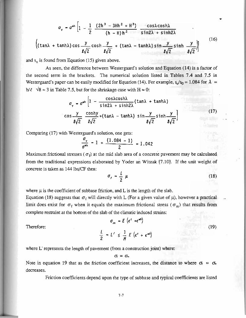
and s, is found from Equation (15) given above.

As seen, the difference between Westergaard's solution and Equation (14) is a factor of

the second term in the brackets. The numerical solution listed in Tables 7.4 and 7.5 in ~ Westergaard's paper can be easily modified for Equation (14). For example, sJso = 1.084 for 2 =

b/l 48 = 3 in Table 7.5, but for the shrinkage case with H = 0:

y coshy Y cos- -+(tanX - tanhX) sin-sinh- 16 1,E

I rJ;r t f i

Comparing (17) with Westergaard's solution, one gets:

Maximum frictional stresses ( of) at the mid slab area of a concrete pavement may be calculated

from the traditional expressions elaborated by Yoder an Witzak [7.10]. If the unit weight of

concrete is taken as 144 lbs/CF then:

where p is the coefficient of subbase friction, and L is the length of the slab. Equation (18) suggests that of will directly with L (For a given value of p), however a practical .-

limit does exist for of when it equals the maximum frictional stress (a,) that results from

complete restraint at the bottom of the slab of the climatic induced strains:

- E (ct **) Om Therefore:

where L' represents the length of pavement (from a construction joint) where:

Oi = a m

Note in equation 19 that as the friction coefficient increases, the distance to where G = om decreases.

Friction coefficients depend upon the type of subbase and typical coefficients are listed

- - - -. .,,

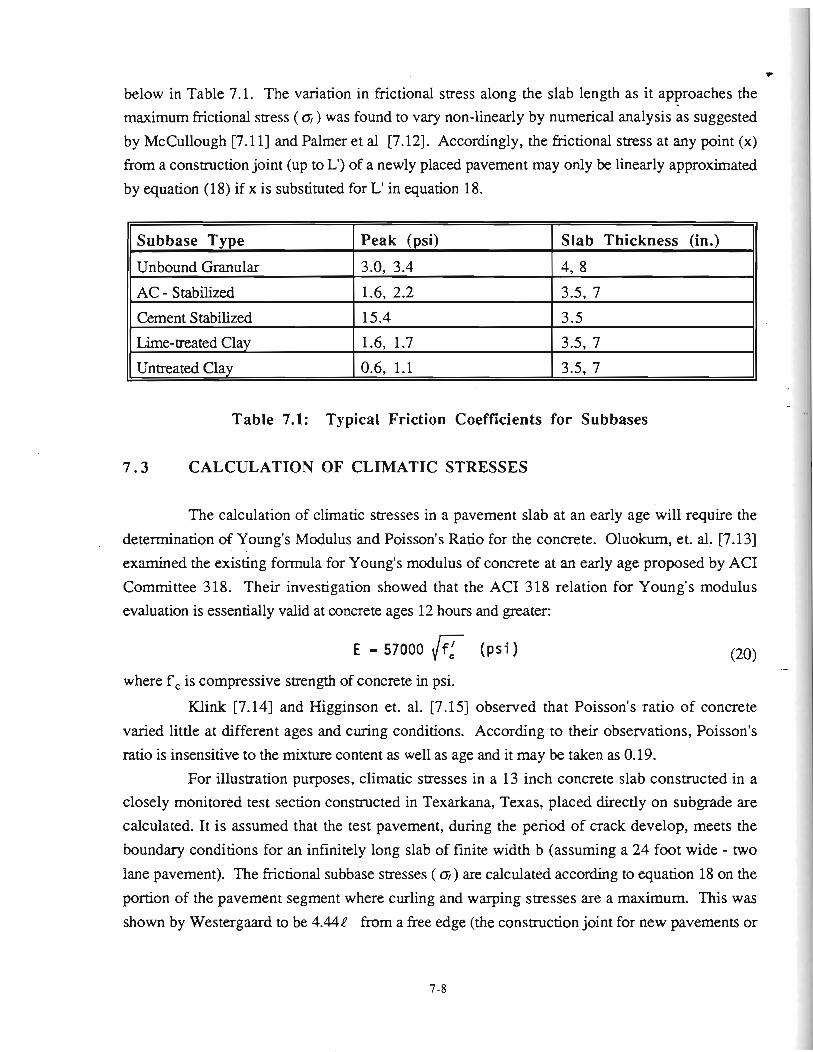
w

* below in Table 7.1. The variation in frictional stress along the slab length as it approaches the

I maximum frictional stress ( a) was found to vary non-linearly by numerical analysis as suggested

1 I by McCullough [7.11] and Palmer et al [7.12]. Accordingly, the fictional stress at any point (x) from a construction joint (up to L') of a newly placed pavement may only be linearly approximated

1 by equation (18) if x is substituted for L' in equation 18.

I

I

Table 7.1: Typical Friction Coefficients for Subbases

7 . 3 CALCULATION OF CLIMATIC STRESSES

The calculation of climatic stresses in a pavement slab at an early age will require the

determination of Young's Modulus and Poisson's Ratio for the concrete. Oluokum, et. al. [7.13]

examined the existing formula for Young's modulus of concrete at an early age proposed by ACI

Committee 318. Their investigation showed that the ACI 318 relation for Young's modulus evaluation is essentially valid at concrete ages 12 hours and greater:

E - 57000 (ps i ) (20) .- where f, is compressive strength of concrete in psi.

Klink [7.14] and Higginson et. al. [7.15] observed that Poisson's ratio of concrete

varied little at different ages and curing conditions. According to their observations, Poisson's

ratio is insensitive to the mixture content as well as age and it may be taken as 0.19.

For illustration purposes, climatic stresses in a 13 inch concrete slab constructed in a closely monitored test section constructed in Texarkana, Texas, placed directly on subgrade are

calculated. It is assumed that the test pavement, during the period of crack develop, meets the

boundary conditions for an infinitely long slab of finite width b (assuming a 24 foot wide - two

lane pavement). The frictional subbase stresses ( a,) are calculated according to equation 18 on the

portion of the pavement segment where curling and warping stresses are a maximum. This was

shown by Westergaard to be 4.444 from a free edge (the construction joint for new pavements or

Subbase Type

Unbound Granular

AC - Stabilized

Cement Stabilized

Lime-treated Clay

Untreated Clay

Peak (psi)

3.0, 3.4

1.6, 2.2

15.4

1.6, 1.7

0.6, 1.1

Slab Thickness (in.)

4, 8

3.5, 7

3.5

3.5, 7

3.5, 7

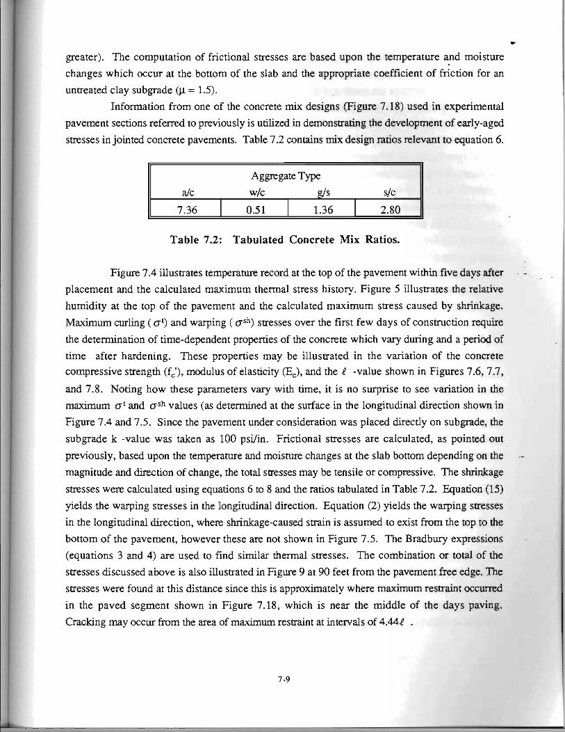
- greater). The computation of frictional stresses are based upon the temperature and moisture

changes which occur at the bottom of the slab and the appropriate coefficient of friction for an

untreated clay subgrade (p = 1.5).

Information from one of the concrete mix designs (Figure 7.18) used in experimental

pavement sections referred to previously is utilized in demonstrating the development of early-aged

stresses in jointed concrete pavements. Table 7.2 contains mix design ratios relevant to equation 6.

Table 7.2: Tabulated Concrete Mix Ratios.

Figure 7.4 illustrates temperature record at the top of the pavement within five days after - -

placement and the calculated maximum thermal stress history. Figure 5 illustrates the relative

humidity at the top of the pavement and the calculated maximum stress caused by shrinkage.

Maximum curling ( at) and warping ( ash) stresses over the first few days of construction require

the determination of time-dependent properties of the concrete which vary during and a period of

time after hardening. These properties may be illustrated in the variation of the concrete compressive strength (f,'), modulus of elasticity (E,), and the 1 -value shown in Figures 7.6,7.7,

and 7.8. Noting how these parameters vary with time, it is no surprise to see variation in the

maximum at and a s h values (as determined at the surface in the longitudinal direction shown in

Figure 7.4 and 7.5. Since the pavement under consideration was placed directly on subgrade, the I

subgrade k -value was taken as 100 psilin. Frictional stresses are calculated, as pointed out I

previously, based upon the temperature and moisture changes at the slab bottom depending on the -- magnitude and direction of change, the total stresses may be tensile or compressive. The shrinkage

stresses were calculated using equations 6 to 8 and the ratios tabulated in Table 7.2. Equation (15) I

yields the warping stresses in the longitudinal direction. Equation (2) yields the warping stresses

in the longitudinal direction, where shrinkage-caused strain is assumed to exist from the top to the

bottom of the pavement, however these are not shown in Figure 7.5. The Bradbury expressior (equations 3 and 4) are used to find similar thermal stresses. The combination or total of th

stresses discussed above is also illustrated in Figure 9 at 90 feet from the pavement free edge. The

stresses were found at this distance since this is approximately where maximum restraint occurred

in the paved segment shown in Figure 7.18, which is near the middle of the days paving

Cracking may occur from the area of maximum restraint at intervals of 4.441 .

7 . 4 SAWCUT SPACING DEPTH REQUIREMENTS

To determine the spacing of the transverse joint locations or sawcuts for a newly placed

concrete pavement, the assumption that a newly paved pavement in the uncracked condition is

infinitely long applies. Therefore, the maximum total climatic stress (as described above) is

calculated at approximately 4.441 from a free end of the pavement or a crack as predicted by

Westergaard analysis. The position of maximum stress may vary for early-aged concrete since P changes during this period of time. As the concrete ages, maximum stress locations stabilizes

typically at 13 to 16 foot intervals, depending on the subbase type, which provides some guidance

as to the recommended joint spacing for design and construction purposes.

The same analysis may apply to the spacing of the longitudinal sawcut locations,

however the focus in this instance is normally to examine the suitability of standard joint locations

which often times serve as lane dividers. In a two-lane pavement, the longitudinal tensile stress at .

the pavement top is calculated at the longitudinal joint location (such as along the center line where -

the pavement is divided to two 12-ft-wide strips), the total tensile stress a, is reduced by a factor

of 50% according to equation (16) which, in this case, is below the tensile strength of concrete.

7.5 THEORY AND APPLICATION OF FRACTURE MECHANICS

The analysis of notched concrete pavement slab based on fracture mechanics

incorporates the stresses generated by temperature and shrinkage affects which are applied as

loads. Important material parameters as identified by the Size Effect Law [7.16] are determined

based on notched beam tests. The notch depth is great enough such that the crack will develop

quickly and extend to the slab bottom under the applied stress. Through fracture tests, fracture parameters KIf and Cf at early ages of concrete have been obtained for concretes of different coarse --

aggregates 17.171. The KIf is the critical stress intensity factor for a specimen of infinite dimension

(in depth), in which linear elastic fracture mechanics (LEFM) applies to the analysis thereof. With respect to the application of KIf to a concrete slab, LEFM still can be applied to determine a

sufficient notch depth even though a concrete slab is not infinitely large. This is because the

nominal strength of an infinite specimen is lower than the nominal strength which is predicted for -

the finite specimen with linear elastic fracture mechanics (LEFM) based on KIf as the failure

criterion (see Figure 7.10).

As in linear mechanics, the superposition principle can be used for the stress intensity

when a specimen or structure is subjected to more than one load. The stress intensity factor due to

any load can always be expressed as follows:

K, - 0 6 N(o) (20)

*

where s is defined as the nominal stress, a is the crack length, and N ( o ) is a non-dimensional function of the ratio, o , of the crack length (a) to the specimen dimension, d. N(w) is called

nominal stress intensity factor. The beam depth (pavement thickness h) is usually taken as the

dimension d. The nominal stress intensity factor is dependent on the specimen geometry, but

independent of the specimen size. The nominal stress intensity factor N ( o ) for the simple tension

[7.18] is:

N ( o ) = 1.122 - 0.321 OI + 10.55002 - 21.710013 + 30.382 0 4 (21) where o = a/h (Figure 7.1 1 (a)) and the nominal stress s is the load intensity. For the pure

bending [7.10]:

N ( o ) = 1.122 - 1.400 + 7.33 a 2 - 13.08 w3 + 14.0 a4 (22) where o = a/h (Figure 7.1 1 (b)) and the nominal stress a is the maximum in the distributed load.

Note that these two formulas are for the geometry with top and bottom surfaces free from external

forces. Figure 7.12 shows the tendencies of curling and warping due to the temperature gradient

and shrinkage, where Equation (22) is approximately valid. The double edge notched test

specimen (Figure 7.13) can be used to develop the fracture analysis as this specimen is somewhat

representative of a slab configuration since the centerline in this symmetrical specimen does not

move in the vertical direction. The following equation is valid for o = (ah) < 0.7:

N ( o ) = 1-12 + 0.203 o - 1.197 0.12 + 1.930 0 3 (23) where the nominal stress a is the load intensity. Equations 22 and 23 are useful in applying, the

stress field induced by climatic affects to the determination of the stress intensity given in equation

20 by dividing the stress field into components of tensile forces and bending moments. The finite

element analysis in this study has shown that replacement of the distributed load on a specimen in

simple tension by its resultant---a concentrated load acting along the specimen centerline does not yield significant change in the KI value, particularly where the specimen length is four times the

thickness. Equation (22) can be applied to pure bending loads other than that shown in Figure

7.11(b) by substituting a = 6M/h2. Accordingly, the shrinkage-induced stresses (Figure 7.3) are

transformed to a tensile force and a bending moment. For instance, if H = h/2, the resultant tensile

force is h ash18 then Equation (23) can be used in equation (20) by substituting a = osh/8 (the

resultant force). The bending moment, M = (5196) a s h h2, yields a = (5116) ash in which Equation (22) can be used for KI equation (20) with a due to the bending moment.

Determination of the stress intensity as given in equation (20) can be accomplished, for a

given set of climatic conditions, at anticipated sawcut locations (Figure 7.14) to generate sawcut depth guidelines shown in Figure 7.15. The KI values with different notch (sawcut) depths under

temperature and shrinkage stresses are determined with equations (22) and (23). Figure 7.15 also gives the KI values for the temperature difference t of lWF, 20°F, 40°F, and 50'F between the

pavement top and bottom, with the same shrinkage-induced stresses.

w

The type of coiuse aggregate is also important. When the critical stress intensity factor KIf equals or exceeds the fracture toughness, (typical for river gravel concrete at an age of 12

hours), a sawcut depth of 1 inch is enough if temperature difference is not less than 20'F. When

Klr = 800 psi &(typical for limestone concrete at an age of 12 hours), a sawcut depth of 1.7

inches is enough if the temperature difference is not less than 30'F. Noting the change in stress

intensity in comparison to fracture toughness, for the given climatic conditions, one can develop a

sense for appropriate sawcut timing to control cracking at the sawcut notches.

Similar analysis can be applied to the climatic stresses and sawcut depth requirements for

longitudinal joints with the exceptions being the length of the slab (transversely) and the location of

the longitudinal joints as previously noted

7 .6 EFFECTS OF PAVEMENT THICKNESS ON THE SAWCUT DEPTH

The required sawcut depth for pavements of different thicknesses is best illustrated by - -

considering two pavements of different thicknesses under temperature and shrinkage conditions

(where the temperature at the top has decreased by t'F while temperature at the bottom is assumed

to be unchanged) which cause the pavement slabs to develop the same maximum tensile smss. If

the thermal stress distribution is assumed linear (for the purposes of this discussion) through the

pavement thickness, the thermal stresses can then be decomposed to the axial stress and a bending

stress. Whereas, .in either tension (Equation 26) and bending (Equation 22), the two pavements

have the same nominal stress as determined by Equation (20). With the same critical stress

intensity factor, a larger w ratio is required for thinner pavements. In other words, if the

pavements are of similar geometry (i.e. w is constant) cracking at the notch in the larger slab

requires a smaller nominal stress. This describes the so-called "size effect" of concrete strength.

As an example, analysis has been performed for 8, 10, 12, 15 and 20 inch thick --

pavements. These concrete pavements are assumed to have the same characteristics as listed in Table 7.2 except for the thickness. Calculation results for KIf according to Equations (22) and (23)

are shown in Figure 7.16. For a critical stress intensity factor KIf = 500 psi din, critical ratios of

sawcut depth to pavement thickness and critical sawcut depths for the pavements of different

thicknesses are listed in Table 7.3. Not only does the ratio of the critical sawcut depth to the -

pavement thickness ( a h ) decrease but also does the absolute value of the required sawcut depth

decreases with the thickness. As pointed out earlier, this is attributed to the affect of the size effect

of concrete strength.

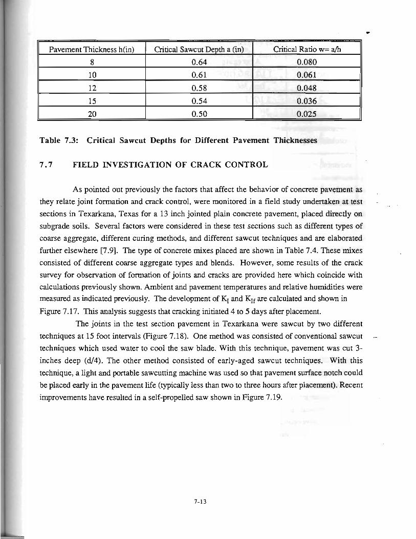
r

w

Table 7.3: Critical Sawcut Depths for Different Pavement Thicknesses

FIELD INVESTIGATION OF CRACK CONTROL

As pointed out previously the factors that affect the behavior of concrete pavement as they relate joint formation and crack control, were monitored in a field study undertaken at test -

sections in Texarkana, Texas for a 13 inch jointed plain concrete pavement, placed directly on

subgrade soils. Several factors were considered in these test sections such as different types of

coarse aggregate, different curing methods, and different sawcut techniques and are elaborated

further elsewhere [7.9]. The type of concrete mixes placed are shown in Table 7.4. These mixes

consisted of different coarse aggregate types and blends. However, some results of the crack

survey for observation of formation of joints and cracks are provided here which coincide with

calculations previously shown. Ambient and pavement temperatures and relative humidities were measured as indicated previously. The development of K1 and KIf are calculated and shown in

I

Figure 7.17. This analysis suggests that cracking initiated 4 to 5 days after placement. !

The joints in the test section pavement in Texarkana were sawcut by two different

techniques at 15 foot intervals (Figure 7.18). One method was consisted of conventional sawcut -- techniques which used water to cool the saw blade. With this technique, pavement was cut 3- inches deep (d/4). The other method consisted of early-aged sawcut techniques. With this

technique, a light and portable sawcumng machine was used so that pavement surface notch could

be placed early in the pavement life (typically less than two to three hours after placement). Recent

improvements have resulted in a self-propelled saw shown in Figure 7.19.

I

7-13

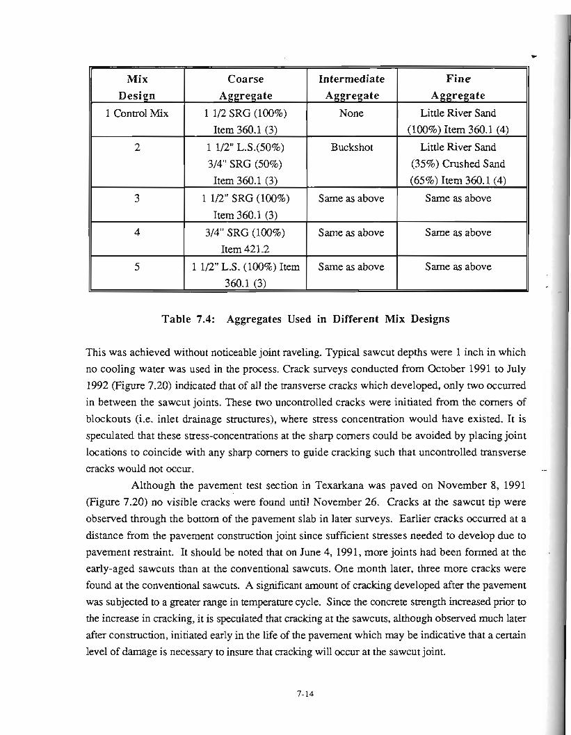
Table 7.4: Aggregates Used in Different Mix Designs

This was achieved without noticeable joint raveling. Typical sawcut depths were 1 inch in which

no cooling water was used in the process. Crack surveys conducted from October 1991 to July

1992 (Figure 7.20) indicated that of all the transverse cracks which developed, only two occurred

in between the sawcut joints. These two uncontrolled cracks were initiated from the comers of

blockouts (i.e. inlet drainage structures), where stress concentration would have existed. It is

speculated that these stress-concentrations at the sharp comers could be avoided by placing joint

locations to coincide with any sharp comers to guide cracking such that uncontrolled transverse

cracks would not occur.

Although the pavement test section in Texarkana was paved on November 8, 1991

(Figure 7.20) no visible cracks were found until November 26. Cracks at the sawcut tip were

observed through the bottom of the pavement slab in later surveys. Earlier cracks occurred at a

distance from the pavement construction joint since sufficient stresses needed to develop due to

pavement restraint. It should be noted that on June 4, 1991, more joints had been formed at the

early-aged sawcuts than at the conventional sawcuts. One month later, three more cracks were

found at the conventional sawcuts. A significant amount of cracking developed after the pavement

was subjected to a greater range in temperature cycle. Since the concrete strength increased prior to

the increase in cracking, it is speculated that cracking at the sawcuts, although observed much later

after construction, initiated early in the life of the pavement which may be indicative that a certain

level of damage is necessary to insure that cracking will occur at the sawcut joint.

Fine Aggregate

Little River Sand

(100%) Item 360.1 (4)

Little River Sand

(35%) Crushed Sand

(65%) Item 360.1 (4)

Same as above

Same as above

Same as above

r

Mix Design

1 Control Mix

2

3

4

5

Coarse Aggregate

1 112 SRG (100%)

Item 360.1 (3)

1 112" L.S.(50%)

3/4" SRG (50%)

Item 360.1 (3)

1 112" SRG (100%)

Item 360.1 (3)

3/4" SRG (100%)

Item 421.2

1 1/2" L.S. (100%) Item

360.1 (3)

Intermediate Aggregate

None

Buckshot

Same as above

Same as above

Same as above

.r

A closer look at the evolution of cracking can be made by examining the results shown in

Figure 7.8. The initial crack interval was on the order of 90 feet or more. Apparently, it is

intervals of this magnitude where the combination of curl, warping, and frictional stresses was

enough to initiate cracking (Figure 7.17). The frictional stress may have been the significant

contribution to crack development given the climatic conditions the paving was accomplished

although a much improved crack pattern developed the following summer. The disadvantage of a

crack pattern developing in this manner is that some joints open wider than designed which may

damage the joint sealant material. It should be pointed out this characteristic was prevalent whether

conventional or early-aged cuttings techniques were used. This condition may be minimized by

using a jointed reinforced concrete pavement type.

It is interesting to note that different types of aggregate affect the fracture properties and

crack development of concrete pavement has shown in Figure 7.21. Cracking at the sawcut tip

occwed more frequently where the concrete coarse aggregate type was river gravel than in that of

crushed limestone concrete. This was also the case in the subsection paved with the concrete that

used a blend of crushed limestone and river gravel as the coarse aggregate in comparison to that

paved with the concrete that used crushed limestone only as the coarse aggregate. Lab tests

showed that concrete of crushed limestone had higher flexural and compressive strengths than

concrete of river gravel at early ages [7.11,7.17]. These field results tend to confirm the validity

of using early-aged sawcutting techniques. Although, not expressly addressed in this paper, it

appears that sawcut timing is much more significant than sawcut depth. A shallow notch placed

early in the pavement surface can take advantage of the greater change in temperature and moisture

in the vicinity of the pavement surface (in comparison which results to the changes at a greater

depth) which results in a greater amount of crack damage and subsequent incidence of cracking at

the notches.

7.8 CONCLUSIONS

Modified linear fracture mechanics is applicable to determine sawcut depth for early

cracks. The sawcut depth is dependent on the spacing of the transverse sawcut, the material fracture parameters Kif and Cf, and the stress level in the concrete slab with given geometrical .

conditions. The material fracture parameters vary with time especially at early ages of concrete.

Field observation has found that late cracks are also initiated by the sawcutting notches. However,

the propagation of these cracks may be caused by long-term fluctuating thermal and moisture

loads, for which further research is needed.

The reduction of sawcut depth (less than d/3 or d/4) at concrete joints by early-age

sawcut or placement techniques will take advantage of the greater change in moisture anL

w

temperature in the concrete at the pavement surface (in comparison to the change at d/3 or d/4) to

initiate cracking at the notches at a greater incidence than otherwise. Therefore, the control of

cracking of concrete pavement should be improved. Field surveys indicate that under some

circumstances (such as cool weather paving conditions) transverse cracks at the sawcut notches

may initiate much later after placement. On a preliminary basis, this study indicates that it is

reasonable to use notch depths on the order of one inch to initiate cracking at the pavement surface

which is significantly less than the traditional d/4 or d.3.

7.8.1 Acknowledgments Appreciation is extended to the Texas DOT and FHWA for the financial support under

Project 1244. This paper is based on portions of the results of this study.

7 . 9 REFERENCES

1 . Emborg, M., (1989), "Thermal Stresses in Concrete Structures at Early Ages," Doctoral

Thesis, LuleA University of Technology, LuleA, Germany.

2. Richardson, J. M., and Armaghani, J. M., (1987), "Stress Caused by Temperature Gradient

in Portland Cement Concrete Pavements," Transportation Research Record 1121,

Transportation Research Board, Washington, D. C.

3. Westergaard, H. M., (1927), "Analysis of Stresses in Concrete Pavements Due to

Variations of Temperature," Proceedings of the Sixth Annual Meeting, Highway Research

Board. .-

4. Bradbury, R. D., (1938), "Reinforced Concrete Pavements," Wire Reinforcement Institute,

Washington, D. C.

5 . Tang, T., and Zollinger, D.G., and Senadheera, S, (1992), "Analysis of Concrete Curling

in Concrete Slabs," Submitted to the Journal of Transportation Engineerin%, September

1993, Paper accepted by ASCE.

6 . ~az'ant, Z. P., Wu, S. T., (1974), "Creep and Shrinkage Law for Concrete at Variable

Humidity," Journal of the E n ~ n e e r i n ~ Mechanics Division, Vol. 100.

7. ~az'ant , Z. P., Panula, L., (1978), "Practical Prediction of Time-Dependent Deformation of

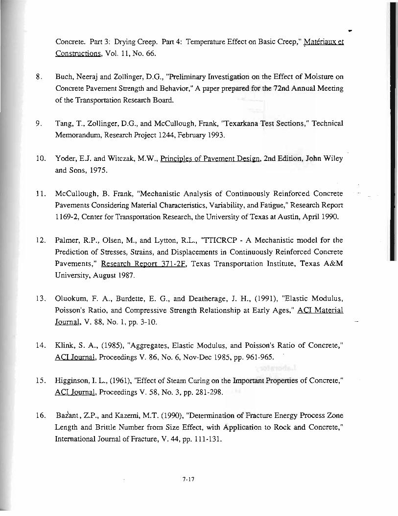
w

Concrete. Part 3: Drylng Creep. Part 4: Temperature Effect on Basic Creep," Materiaux et

Constructions, Vol. 1 1, No. 66.

8. Buch, Neeraj and Zollinger, D.G., "Preliminary Investigation on the Effect of Moisture on

Concrete Pavement Strength and Behavior," A paper prepared for the 72nd Annual Meeting

of the Transportation Research Board.

9. Tang, T., Zollinger, D.G., and McCullough, Frank, "Texarkana Test Sections," Technical

Memorandum, Research Project 1244, February 1993.

10. Yoder, E.J. and Witczak, M.W., Principles of Pavement Design, 2nd Edition, John Wiley

and Sons, 1975.

11. McCullough, B. Frank, "Mechanistic Analysis of Continuously Reinforced Concrete

Pavements Considering Material Characteristics, Variability, and Fatigue," Research Report

1169-2, Center for Transportation Research, the University of Texas at Austin, April 1990.

12. Palmer, R.P., Olsen, M., and Lytton, R.L., "'ITICRCP - A Mechanistic model for the

Prediction of Stresses, Strains, and Displacements in Continuously Reinforced Concrete

Pavements," Research Report 37 1 -2F, Texas Transportation Institute, Texas A&M

University, August 1987.

13. Oluokum, F. A., Burdette, E. G., and Deatherage, J. H., (1991), "Elastic Modulus,

Poisson's Ratio, and Compressive Strength Relationship at Early Ages," ACI Material

Journal, V. 88, No. 1, pp. 3-10.

14. Klink, S. A., (1985), "Aggregates, Elastic Modulus, and Poisson's Ratio of Concrete,"

ACI Journal, Proceedings V. 86, No. 6, Nov-Dec 1985, pp. 961-965.

15. Higginson, I. L., (1961), "Effect of Steam Curing on the Important Properties of Concrete,"

ACI Journal, Proceedings V. 58, No. 3, pp. 281-298.

16. ~az'ant, Z.P., and Kazemi, M.T. (1990), "Determination of Fracture Energy Process Zone

Length and Brittle Number from Size Effect, with Application to Rock and Concrete,"

International Journal of Fracture, V. 44, pp. 1 1 1-13 1.

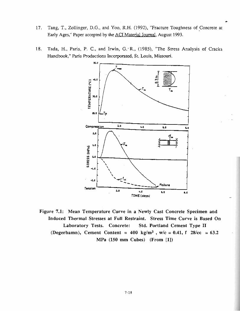
w

17. Tang, T., Zollinger, D.G., and Yoo, R.H. (1992), "Fracture Toughness of Concrete at

Early Ages," Paper accepted by the ACI Material Journd, August 1993.

18. Tada, H., Paris, P. C., and Irwin, G:R., (1985), "The Stress Analysis of Cracks

Handbook," Paris Productions Incorporated, St. Louis, Missouri.

La 4.0 b O L O

TIME (daysl

Figure 7.1: Mean Temperature Curve in a Newly Cast Concrete Specimen and Induced Thermal Stresses at Full Restraint. Stress Time Curve is Based On

Laboratory Tests. Concrete: Std. Portland Cement Type II (Degerhamn), Cement Content = 400 kg/m3 , w/c = 0.41, f 28/cc = 63.2

MPa (150 mm Cubes) (From [I])

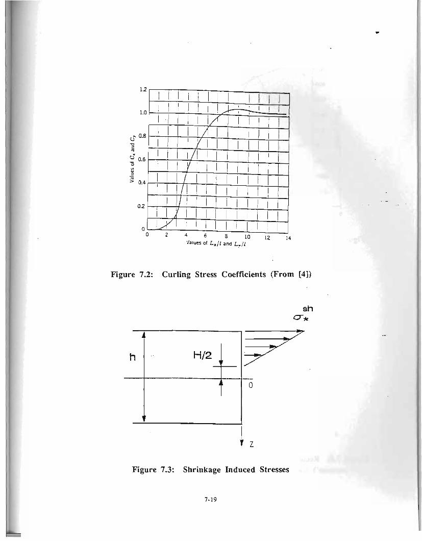
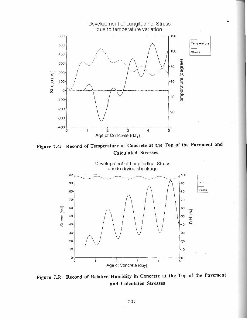
Development of Longitudinal Stress due to temperature variation

600.120 Temperature

Slress

:" , v , , 1 -400

1 2 3 4 5 0

Age of Concrete (day)

Figure 7.4: Record of Temperature of Concrete at the Top of the Pavement and Calculated Stresses

Development.of Longitudinal Stress due to drying shrinkage

100 --..- I .- -..- -----. .-.--. ----.. - .-.--*.. ,*- .--- _,. C----. ... ...--- .--.._.- 100 --.____..-. ---.

0. I I I

0 1 3 4 I

2 I lo

5 Age of Concrete (day)

Figure 7.5: Record of Relative Humidity in Concrete at the Top of the Pavement and Calculated Stresses

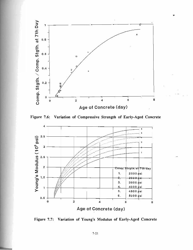
)r = 1 -

n w

E w - b

0.8 - a Ai - w m

0.6 - V)

6. - E O 0.4 - 0 \ - k w

0.2 - .CI

U) - d. E 0 I I I I I I

0 0 2 4 6 8 0

Age of Concrete (day) I

Figure 7.6: Variation of Compressive Strength of Early-Aged Concrete

0 2 4 6 8

Age of Concrete (day)

Figure 7.7: Variation of Young's Modulus of Early-Aged Concrete

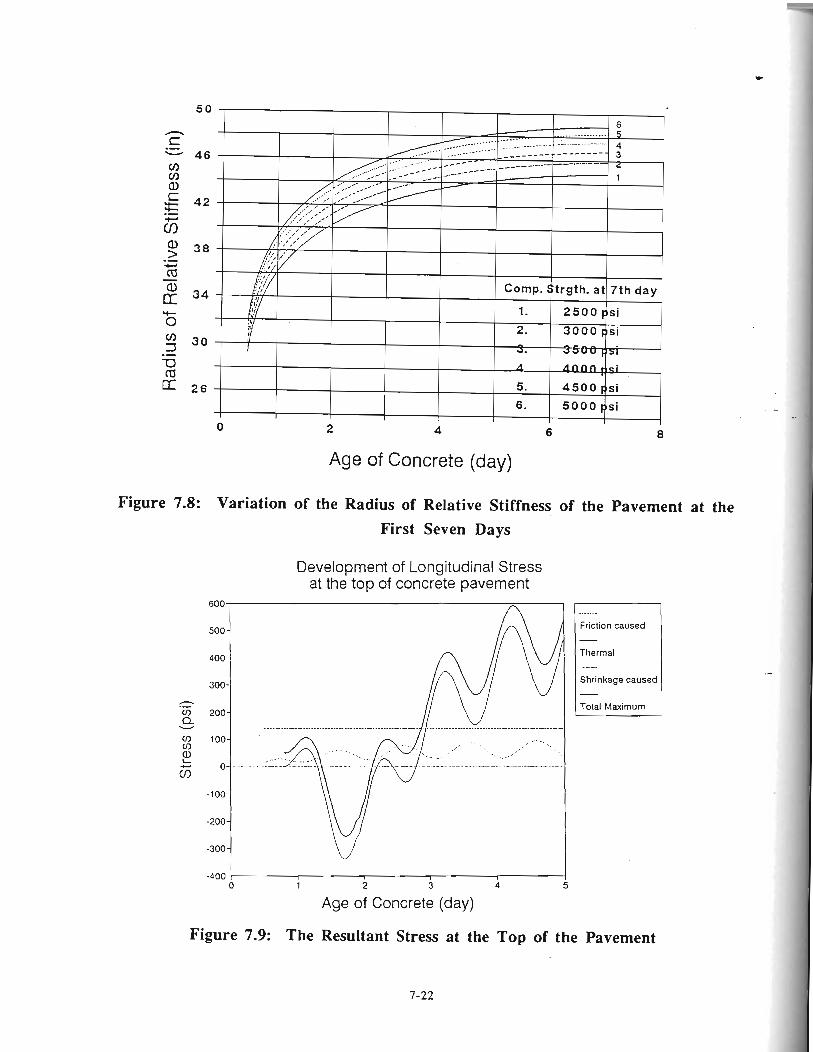
Age of Concrete (day)

Figure 7.8: Variation of the Radius of Relative Stiffness of the Pavement at the First Seven Days

Development of Longitudinal Stress at the top of concrete pavement

Friction caused

Thermal

Shrinkage caused

Total Maximum

Age of Concrete (day)

Figure 7.9: The Resultant Stress at the Top of the Pavement

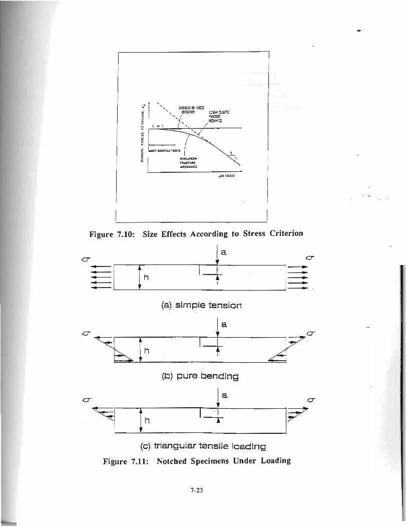
Figure 7.10: Size Effects According to Stress Criterion

(a) simple tension

(b) pure bending

(c) triangular tensile loading

Figure 7.11: Notched Specimens Under Loading

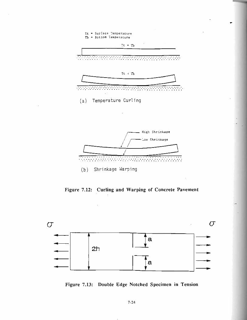
Tt = Surface Teztperacure = 3occom Temperacure

( a ) ~ e r n p e r a t u r e Cur l i n g

,,,- Hisn Shrinkage

( b ) S h r i n k a g e Warping

Figure 7.12: Curling and Warping of Concrete Pavement

Figure 7.13: Double Edge Notched Specimen in Tension

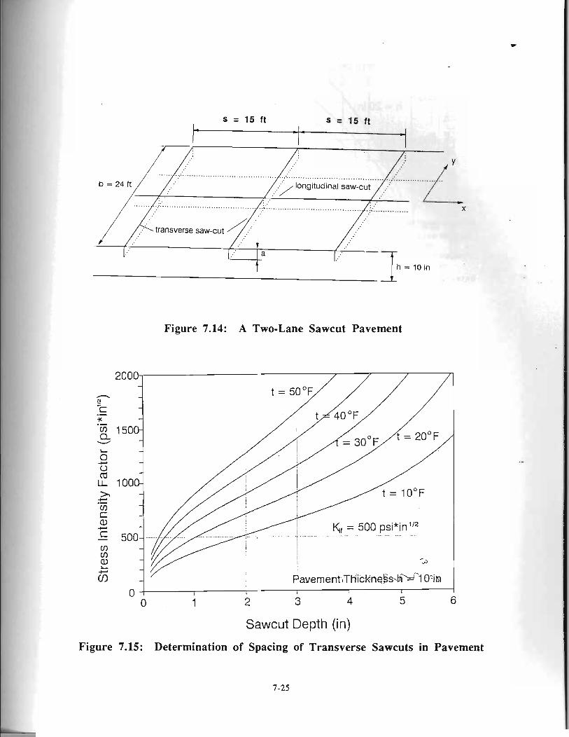
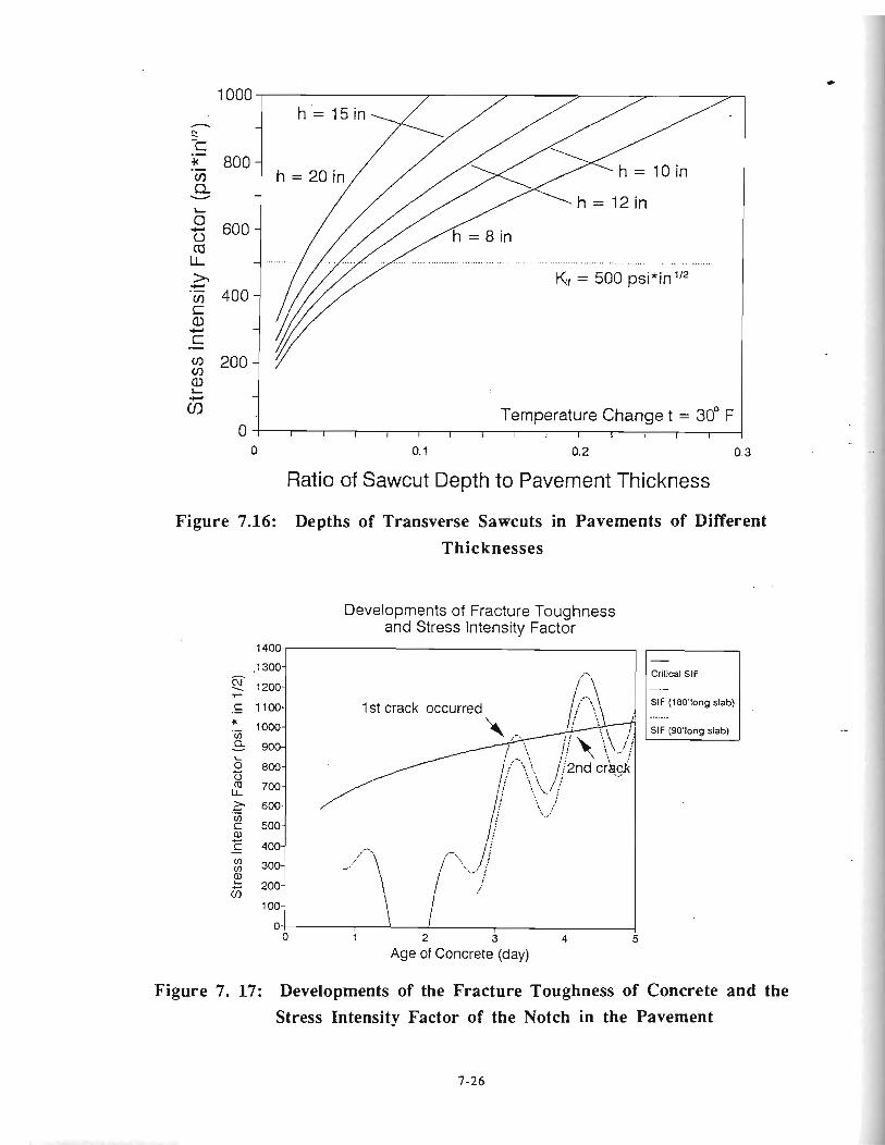
h C! -c .- * .- cn Q w

0' + 0 a U, > + .- (I) C a, + c (I) m 2 Y

Temperature Change t = 30" F 0 1 I I I I I I I 1 I I I I I I

Ratio of Sawcut Depth to Pavement Thickness

Figure 7.16: Depths of Transverse Sawcuts in Pavements of Different Thicknesses

Developments of Fracture Toughness and Stress Intensity Factor

Critical SIF

SIF (180'long slab) -.-.-.- SIF (9O'long slab) E

Figure 7. 17: Developments of the Fracture Toughness of Concrete and the Stress Intensity Factor of the Notch in the Pavement

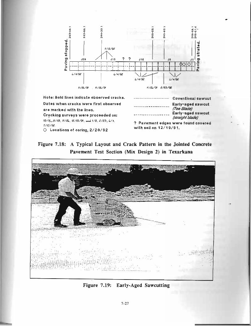
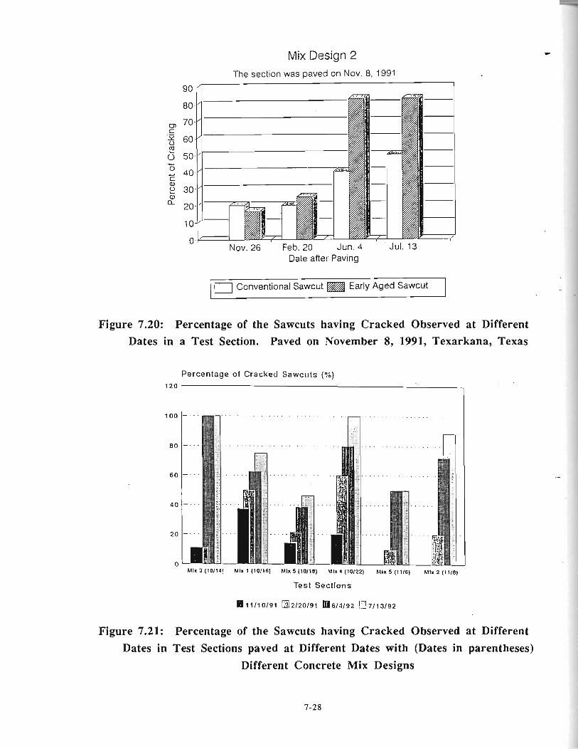
Nov. 26 Feb. 20 Jun. 4 Jul. 13 Date after Paving

( Conventional Sawcut @@j Early Aged Sawcut

Figure 7.20: Percentage of the Sawcuts having Cracked Observed at Different Dates in a Test Section. Paved on November 8, 1991, Texarkana, Texas

Percentage of Cracked Sawcllts (76)

120

1

Mlx 3 (10114! Mlx 1 (10116) Mlx 5 (10118) Mlx 4 (10122) Mlx 5 (1116) Mlx 2 (1118)

Test Sections

811/10/91 02/20/91 86/4/92 0711 3/92

Figure 7.21: Percentage of the Sawcuts having Cracked Observed at Different Dates in Test Sections paved at Different Dates with (Dates in parentheses)

Different Concrete Mix Designs

CHAPTER 8

ANALYSIS OF CONCAVE CURLING IN CONCRETE SLABS

A concrete pavement curls to a concave configuration when it is subjected to a negative

temperature gradient, which results when the temperature at its bottom surface is higher than at its

top surface. A gap may occur between the bottom of the slab and the subgrade if the temperature

gradient is large. This chapter offers an analytical approach to the determination of displacement

and stress distributions for a semi-infinite slab and for an infinitely long slab of a finite width,

which takes into account a gap which may occur under the slab resulting from curling. The -

elementary plate theory is applied to the slab resting on a Winkler foundation.

The analysis for thermal stresses in a curled pavement slab developed by Westergaard

assumes a spring model to represent the subgrade support as a Winkler foundation. The approach

adopted by Westergaard is not valid for the case where a gap exists, although it has been widely

employed without respect to the effect of the gap on the resulting stress distribution. This study

examines a critical temperature difference between the bottom and the top slab surfaces at the

threshold of gap formation at the slab/subgrade interface in terms of the concrete elastic constants

and density, the thermal expansion coefficient of the concrete, thickness of the pavement, and the

modulus of the foundation support. If the temperature difference is below the critical value, it is

shown that Westergaard's solutions are valid Based on the solutions presented herein, correction

of the coefficients in Bradbury's approximate formula for the maximum stress in a finite pavement

are suggested.

8.1 INTRODUCTION .-

A concrete slab will tend to curl when it is subjected to a temperature gradient extending

vertically through the slab thickness. The tendency to curl induces smsses in the pavement as the

pavement is restrained by its weight and the support pressures from the subgrade (or foundation).

The thermally induced stress caused by such interaction can be a significant factor in contributing

to early pavement cracking. This set of circumstances may be critical particularly within a few

hours after placement since concrete is in the early stage of hydration such that the strength may be insufficient to prevent cracking. Research has shown [8.1] that temperature rise caused by

hydration does not immediately produce thermal stresses because of the process of stress relaxation

or creep in the concrete. Thennal stresses arise when the temperature drops after its peak value and

the concrete has taken on a set. However, the temperature gradient which causes the slab to curl,

as affected by the heat of hydration, could be greater than that caused only by the effect of ambient

temperature and solar radiation only. Therefore, analysis of thermal strains, as gene&ted from all

sources of heat, is especially important for a curled slab at a very early concrete age.

Westergaard's solution [8.2] has been widely used in estimating thermal stresses in curled

concrete pavements [8.3],[8.4]. In his solution, temperature change is assumed to be linear

through the thickness of the pavement, the concrete is assumed linear elastic, and a spring model is

used to define an elastic subgrade or a Winkler foundation. However, when the temperature

difference between the bottom surface and the top surface of the pavement slab exceeds a critical

value, the pavement may be so curled that a length of it near the slab edge separates from the

subgrade and a gap between the slab bottom and the subgrade results. Although no mutual action

exists between the separated portion of the slab and the subgrade, the spring model in'

Westergaard's solutions is assembled over the entire slab bottom. In this chapter, a modification to

the Westergaard analysis is suggested which provides a separation of the spring model from the portion of the slab which is free from the subgrade so as to more appropriately reflect actual slab

behavior. The Westergaard analysis provides expressions for displacement and stress distributions

for a semi-infinite slab and a infinitely-long slab of a finite width. For a slab of finite dimensions,

Bradbury 18.51 suggested an approximate formula to estimate the maximum stress, where two

coefficients were given based on the Westergaard analysis. Consequently, modifications of the

Westergaard analysis can be encompassed within modifications for curled slabs which all account

for slab lift off at the slab edge.

8.2 BASIC EQUATIONS

Solutions of this study are, in a general sense, solutions to thermal stress and displacement

distributions in an elastic plate resting on a Winkler foundation and consequently are applicable to .-

concrete pavements.

The subgrade reaction of a Winkler foundation is expressed as [8.5]:

q = -kw (1)

where q is the subgrade stress on a unit area, w is the displacement of the slab, and constant k is

called the Foundation Modulus. The minus sign in Equation (1) indicates that the reaction occurs

in the opposite direction of displacement w. When the temperature in a pavement slab is unifmly

distributed, the slab theoretically remains planar that is accompanied with a uniform vertical

subgrade displacement. By denoting p and h as the density and thickness of the concrete slab

respectively, one obtains the vertical displacement due to the weight of the slab as: ph wo =- k

*

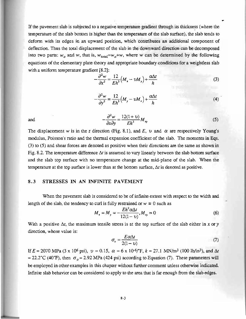
If the pavement slab is subjected to a negative temperature gradient through ics thickness (where the

temperature of the slab bottom is higher than the temperature of the slab surface), the slab tends to

deform with its edges in an upward position, which contributes an additional component of

deflection. Thus the total displacement of the slab in the downward direction can be decomposed into two parts: w, and w, that is, w,~=w,+w, where w can be determined by the following

equations of the elementary plate theory and appropriate boundary conditions for a weightless slab

with a uniform temperature gradient [8.2]:

and

a2w 12 --=- cult dx2 Eh3 (M, - V M , ) + ~

a2w 12 --=- cult

2 ~ h 3 (MY - V M ~ ) +- h

The displacement w is in the z direction (Fig. 8. I), and E, v and a are respectively Young's

modulus, Poisson's ratio and the thermal expansion coefficient of the slab. The moments in Eqs.

(3) to (5) and shear forces are denoted as positive when their directions are the same as shown in

Fig. 8.2. The temperature difference At is assumed to vary linearly between the slab bottom surface

and the slab top surface with no temperature change at the mid-plane of the slab. When the

temperature at the top surface is lower than at the bottom surface, At is denoted as positive.

8.3 STRESSES IN AN INFINITE PAVEMENT

When the pavement slab is considered to be of infinite extent with respect to the width and .-

length of the slab, the tendency to curl is fully restrained or w = 0 such as

With a positive At, the maximum tensile stress is at the top surface of the slab either in x ory

direction, whose value is:

a, = EaAt 2(1- v)

If E = 2070 MPa (3 x 106 psi), v = 0.15, a = 6 x 10-6/'F, k = 27.1 MN/m3 (100 Ib/in3), and At = 22.2"C (40°F), then a, = 2.92 MPa (424 psi) according to Equation (7). These parameters will

be employed in other examples in this chapter without further comment unless otherwise indicated

Infinie slab behavior can be considered to apply to the area that is far enough from the slab edges.

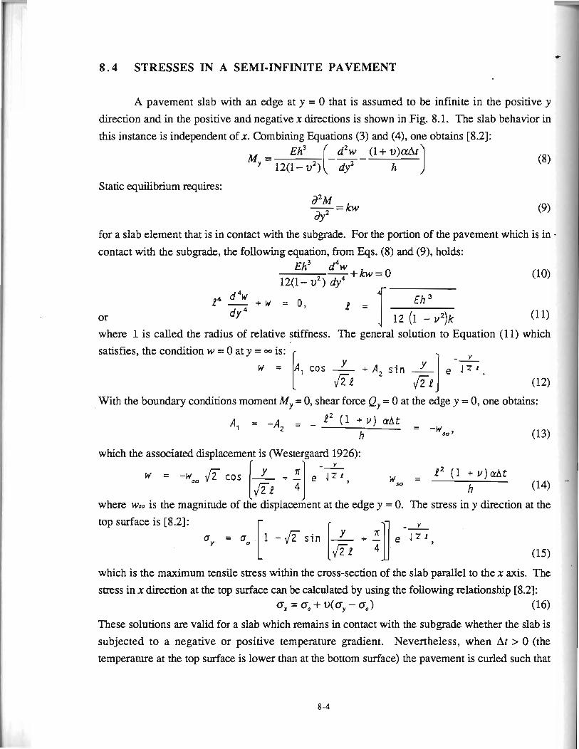
8.4 STRESSES IN A SEMI-INFINITE PAVEMENT

A pavement slab with an edge at y = 0 that is assumed to be infinite in the positive y direction and in the positive and negative x directions is shown in Fig. 8.1. The slab behavior in

this instance is independent of x. Combining Equations (3) and (4), one obtains 18.21: d2w (1+ v)aAt " (---

My = 12(1- v2) dy2 h (8)

Static equilibrium quires :

for a slab element that is in contact with the subgrade. For the portion of the pavement which is in - contact with the subgrade, the following equation, from Eqs. (8) and (9), holds:

where 1 is called the radius of relative stiffness. The general solution to Equation (11) which

satisfies, the condition w = 0 at y = - is:

I I - Y

Y - + A 2 s i n - e I7f.

6 1 (12) With the boundary conditions moment My = 0, shear force Q, = 0 at the edge y = 0, one obtains:

which the associated displacement is (Westergaard 1926): - - Y - W = - s [ + ] 4 7 1 , W+q - - P2 (1 + v)aAt

(14) .-

h where wso is the magnitude of the displacement at the edge y = 0. The stress in y direction at the

top surface is [8.2]: - Y - e J 7 I 7

which is the maximum tensile stress within the cross-section of the slab parallel to the x axis. The

smss in x direction at the top surface can be calculated by using the following relationship [8.2]: a, = a, + v(ay - a,) (16)

These solutions are valid for a slab which remains in contact with the subgrade whether the slab is

subjected to a negative or positive temperature gradient. Nevertheless, when At > 0 (the

temperature at the top surface is lower than at the bottom surface) the pavement is curled such that

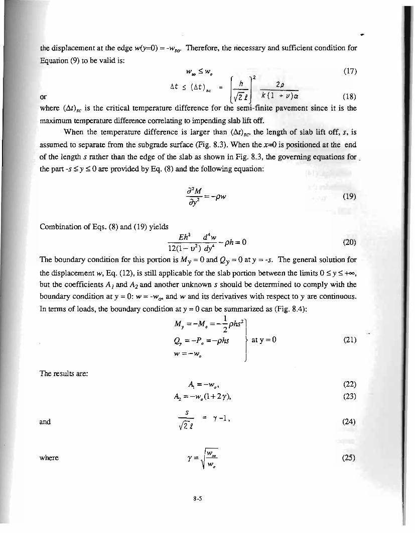
le displacement at the edge w(y=O) = -w,, Therefore, the necessary and sufficient condition for

lation (9) to be valid is:

w, * wo 2

(17)

A t 5 ( A t : * = [&I 2~

or k(l + v ) a (18) where (At), is the critical temperature difference for the semi-finite pavement since it is the

maximum temperature difference correlating to impending slab lift off. When the temperature difference is larger than (Az),,, the length of slab lift off, s, is

assumed to separate from the subgrade surface (Fig. 8.3). When the x=O is positioned at the end

of the length s rather than the edge of the slab as shown in Fig. 8.3, the governing equations for.

the part -s < y < 0 are provided by Eq. (8) and the following equation:

Combination of Eqs. (8) and (19) yields

The boundary condition for this pomon is My = 0 and Qy = 0 at y = -s. The general solution for

the displacement w, Eq. (12), is still applicable for the slab portion between the limits 0 5 y I +m,

but the coefficients Al and A2 and another unknown s should be determined to comply with the

boundary condition at y = 0: w = -w,, and w and its derivatives with respect to y are continuous.

In tenns of loads, the boundaq condition at y = 0 can be summarized as (Fig. 8.4):

The results are:

and

where

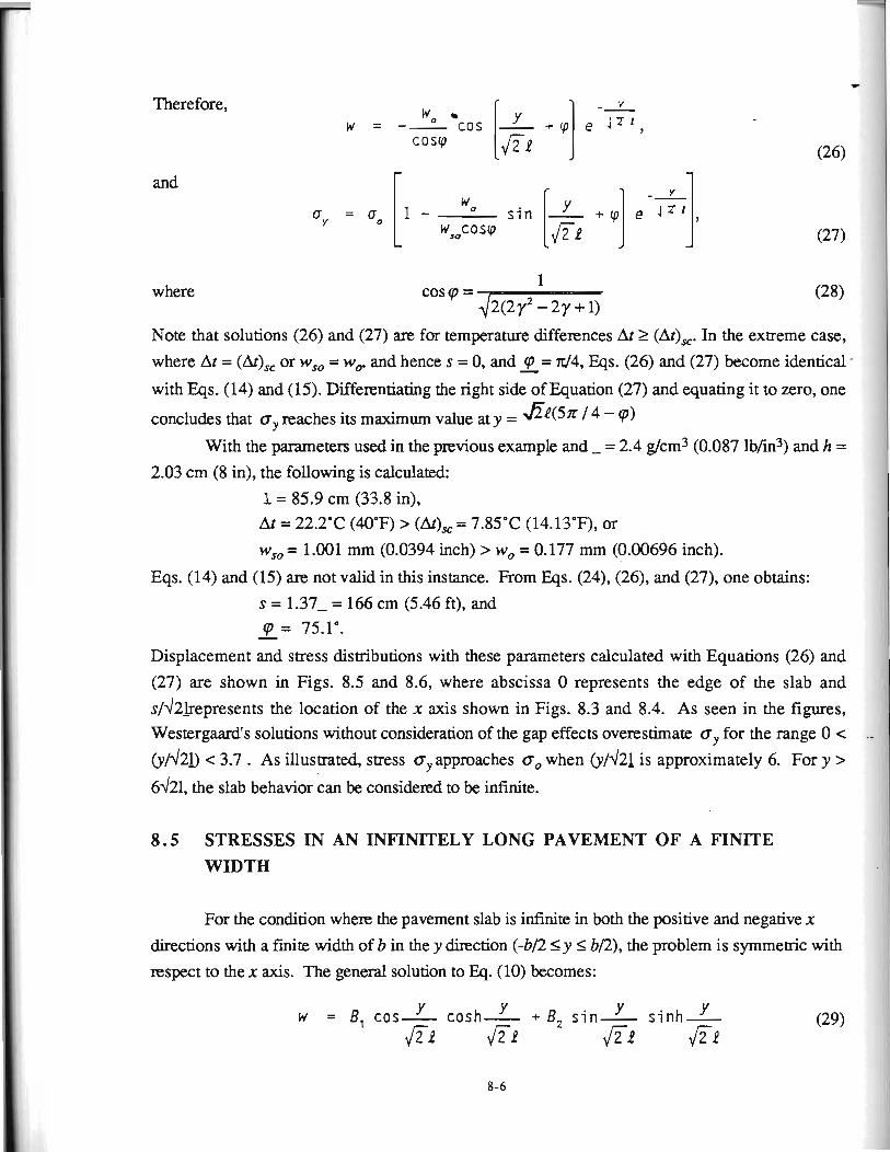
- -- --- - . - -- - - - - - 'r

* Therefore, - Y

W o -

w = - - cos [ +.I i7., cosy

(26)

ITy = ITo

(27)

and

where cos q.3 = ST- 2(2y -2y+l)

(28)

Note that solutions (26) and (27) are for temperature differences At 2 (At),. In the extreme case,

where At = (At), or wso = w, and hence s = 0, and q.3 = 7V4, Eqs. (26) and (27) become identical - - with Eqs. (14) and (15). Differentiating the right side of Equation (27) and equating it to zero, one

concludes that 0, reaches its maximum value at y = 34(5n - 6) With the parameters used in the previous example and - = 2.4 glcm3 (0.087 lbhn3) and h =

2.03 cm (8 in), the following is calculated:

1 = 85.9 cm (33.8 in), At = 22.2-C (40'F) > (At), = 7.85'C (14.13*F), or

wso = 1.00 1 mm (0.0394 inch) > wo = 0.177 mm (0.00696 inch).

Eqs. (14) and (15) are not valid in this instance. From Eqs. (24), (26)- and (27), one obtains:

s = 1.37- = 166 cm (5.46 ft), and

Displacement and stress distributions with these parameters calculated with Equations (26) and

(27) are shown in Figs. 8.5 and 8.6, where abscissa 0 represents the edge of the slab and

s/42~epresents the location of the x axis shown in Figs. 8.3 and 8.4. As seen in the figures, Westergaard's solutions without consideration of the gap effects overestimate oy for the range 0 c ..

~1421) c 3.7 . As illustrated, s a s s oy approaches 0, when @I421 is approximately 6. For y > 6421, the slab behavior can be considered to be infinite.

8.5 STRESSES IN AN INFINITELY LONG PAVEMENT OF A FINITE WIDTH

For the condition where the pavement slab is infinite in both the positive and negative x

directions with a finite width of b in the y direction (-b12 I y I b/2), the problem is symmetric with

respect to the x axis. The general solution to Eq. (10) becomes:

Y Y w = B, COS- cosh- + B, sin- Y sinh- Y f i t 61 m 61

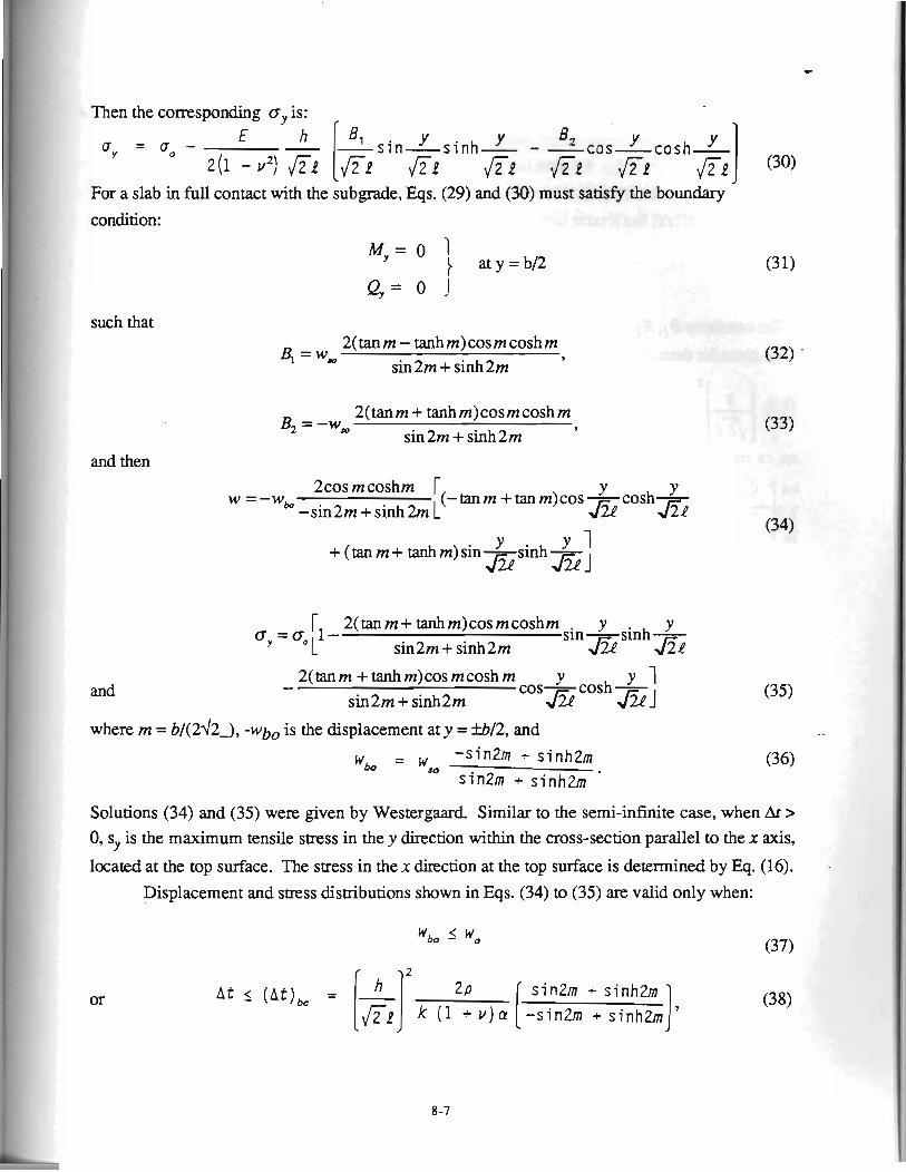
Then the corresponding a, is: ,

ay = a. - E Y Y 8 2 Y sin-sinh- - c o s - cosh- JTn Jih 1 f i 1 f i 1

For a slab in full contact with the subgrade, Eqs. (29) and (30) must satisfy the boundary -

condition:

such that

and then

and

2(tan m - tanh m)cos m cosh m 4 =w, sin 2m + sinh 2m ,

2(tanm + tanh m)cosmcosh m B2 = -w,

sin2m + sinh2m 9

2cosmcoshm r W =-Wh

Y (-tan m + tan m) cos -sin2m + sinh 2m L -

Y + (tan m + tanh m) sin -sinh Y I J2 EJ

r 2(tanm+ tanhm)cos mcoshm y Y

%=oOL'- sin-sinh - sin2m + sinh2m ,I5 a 4

- 2(tan m + tanh m)cos mcosh m y Y 1 cos- cosh -

sin2m + sinh2m fi a 1 (35)

where m = b/(2d2_), -who is the displacement at y = kbD, and

Solutions (34) and (35) were given by Westergaard. Similar to the semi-infinite case, when Af > 0, s,, is the maximum tensile stress in the y direction within the cross-section parallel to the x axis,

located at the top surface. The stress in the x direction at the top surface is determined by Eq. (16).

Displacement and stress distributions shown in Eqs. (34) to (35) are valid only when:

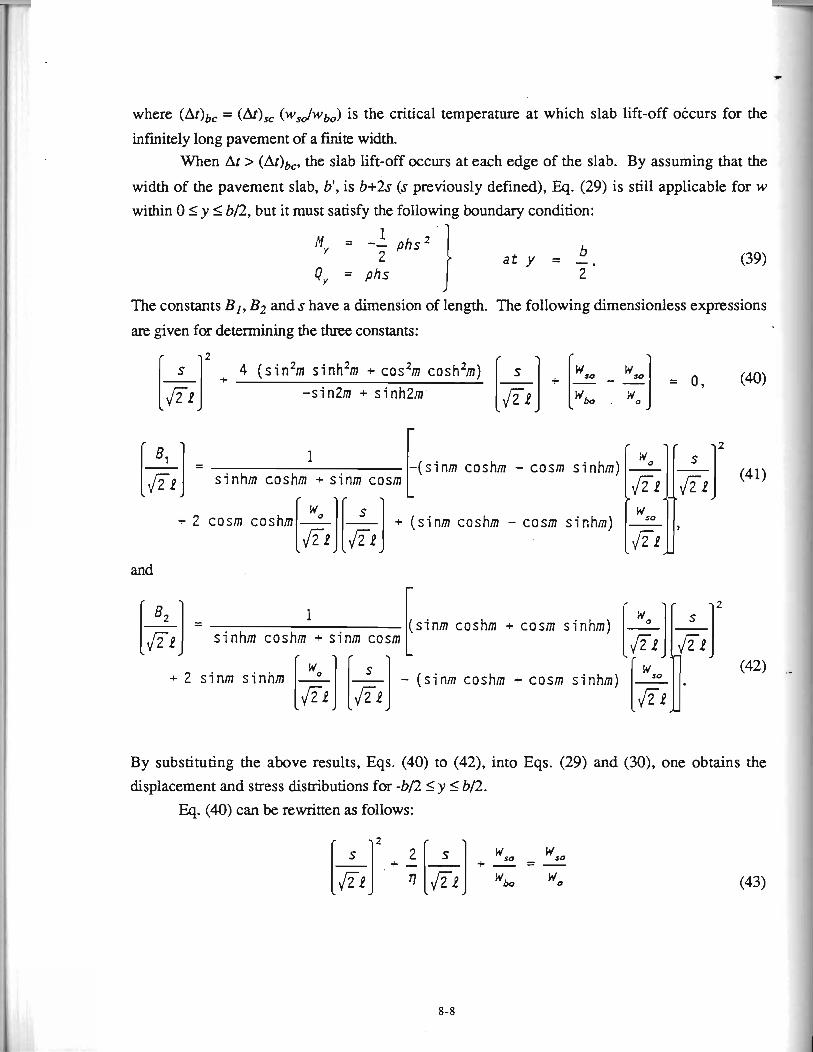
7

where = (At)sc (wSJwbo) is the critical temperature at which slab lift-off &curs for the

infinitely long pavement of a finite width. When At > (&)bc, the slab lift-off occurs at each edge of the slab. By assuming that the

width of the pavement slab, b', is b+2s (s previously defined), Eq. (29) is still applicable for w

within 0 I y 2 b/2, but it must satisfy the following boundary condition:

I The constants BI, B2 and s have a dimension of length. The following dimensionless expressions

I are given for determining the three constants:

I 1 = sinhm coshm + sinm cosm -(sinm coshm - cosm sinhm)

-+ 2 cosm coshm + (sinm coshm - cosm sinhm)

and - 2

1 [$I = sinhm coshm + sinm cosm (sinm coshm + cosm sinhm) I

+ 2 sinm sinhm - (sinm coshm + cosm sinhm)

By substituting the above results, Eqs. (40) to (42), into Eqs. (29) and (30), one obtains the

displacement and stress distributions for -b/2 I y I b/2.

Eq. (40) can be rewritten as follows:

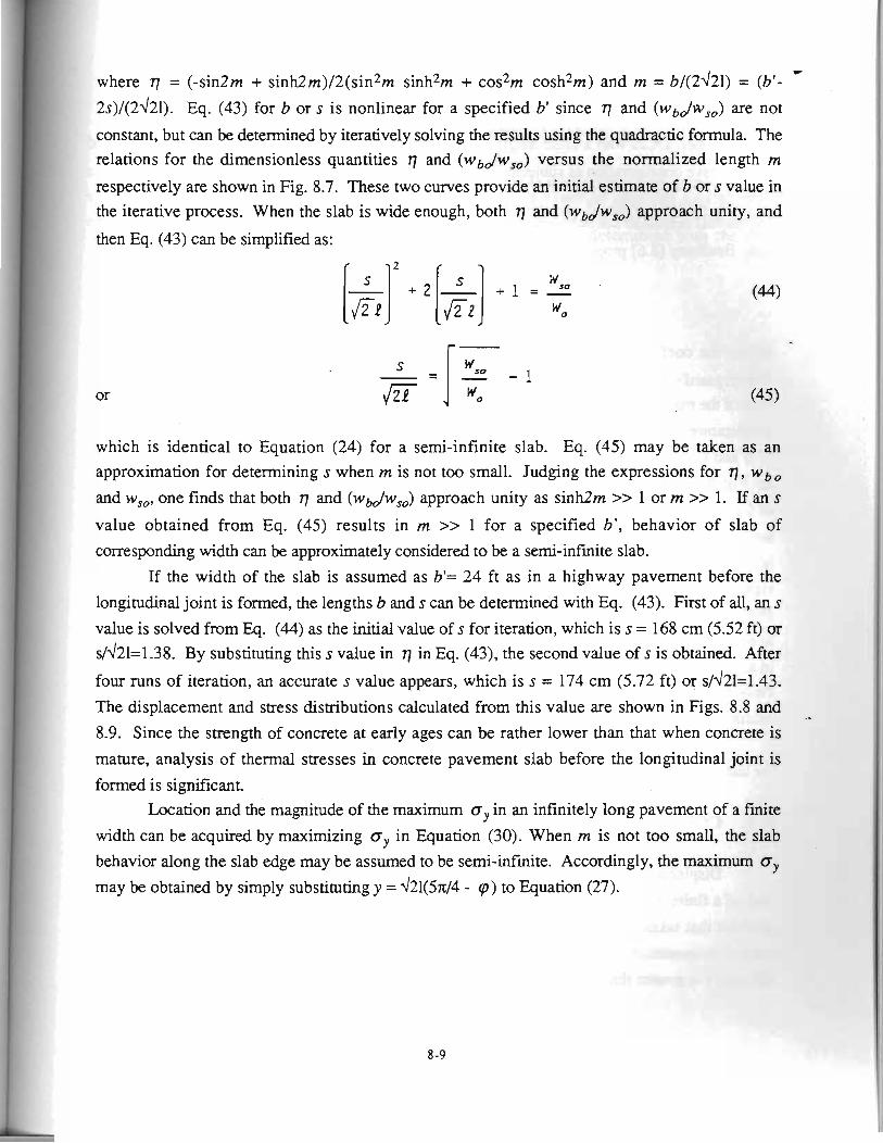
* where q = (-sin2m + sinMm)/2(sin2m sinh2m + cos2m cosh2m) and m = bl(2d21) = (b'-

2s)/(2d21). Eq. (43) for b or s is nonlinear for a specified b' since 7) and (wbJws0) are not

constant, but can be determined by iteratively solving the results using the quadractic formula. The relations for the dimensionless quantities q and (wbJw,,) versus the normalized length m

respectively are shown in Fig. 8.7. These two curves provide an initial estimate of b or s value in the iterative process. When the slab is wide enough, both q and (wbJwso) approach unity, and

then Eq. (43) can be simplified as:

which is identical to Equation (24) for a semi-infinite slab. Eq. (45) may be taken as an approximation for determining s when m is not too small. Judging the expressions for q , wb,

and w,,, one finds that both 77 and (wb,,/wsO) approach unity as sinh2m >> 1 or m >> 1. If an s

value obtained from Eq. (45) results in m >> 1 for a specified b', behavior of slab of

corresponding width can be approximately considered to be a semi-infinite slab.

If the width of the slab is assumed as b'= 24 ft as in a highway pavement before the I i longitudinal joint is formed, the lengths b and s can be determined with Eq. (43). First of all, an s I

value is solved from Eq. (44) as the initial value of s for iteration, which is s = 168 cm (5.52 ft) or I

s/d21=1.38. By substituting this s value in q in Eq. (43), the second value of s is obtained. After

four runs of iteration, an accurate s value appears, which is s = 174 cm (5.72 ft) or s/d21=1.43.

The displacement and stress distributions calculated from this value are shown in Figs. 8.8 and .- 8.9. Since the strength of concrete at early ages can be rather lower than that when concrete is

mature, analysis of thermal stresses in concrete pavement slab before the longitudinal joint is

formed is significant. Location and the magnitude of the maximum cry in an infinitely long pavement of a finit1

width can be acquired by maximizing oy in Equation (30). When m is not too small, the slal behavior along the slab edge may be assumed to be semi-infinite. Accordingly, the maximum a. may be obtained by simply substituting y = d21(5n/4 - q ) to Equation (27).

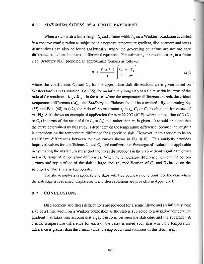
- - - 7

w

8.6 MAXIMUM STRESS IN A FINITE PAVEMENT

When a slab with a finite length L, and a finite width Ly on a Winkler foundation is curled

in a concave configuration as subjected to a negative temperature gradient, displacement and stress I I

distributions can also be found analytically, where the governing equations are not ordinary differential equations but partial differential equations. For estimating the maximum oy in a finite

slab, Bradbury [8.6] proposed an approximate formula as follows:

Q = E a A t C, + YC,

2 [ I $ 1 (46)

where the coefficients C1 and C2 for the appropriate slab dimensions were given based on

Westergaard's stress solution (Eq. (35)) for an infinitely long slab of a finite width in terms of the ratio of the maximum Q / .. In the cases where the temperature difference exceeds the critical

temperature difference (At)& the Bradbury coefficients should be corrected. By combining Eq.

(35) and Eqs. (40) to (42), the ratio of the maximum sy to so, Cl or C2. is obtained for values of m. Fig. 8.10 shows an example of application for At = 22.2"C (40"F), where the relation of C (Cl

or C2) in terms of the ratio of d (= L, or Ly) to 1, rather than m, is given. It should be noted that

the curve determined by this study is dependent on the temperature difference, because the length s

is dependent on the temperature difference for a specified slab. However, there appears to be no significant differences between the two curves shown in Fig. 8.10. This analysis provides improved values for coefficients Cl and C2, and confirms that Westergaard's solution is applicable

in estimating the maximum stress (not the stress distribution) in the slab without significant e m

in a wide range of temperature differences. When the temperature difference between the bottom surface and top surface of the slab is large enough, modification of CI and C2 based on the

solutions of this study is appropriate. .-

The above analysis is applicable to slabs with free boundary conditions. For the case where

the slab edge is restrained, displacement and stress solutions are provided in Appendix I.

8.7 CONCLUSIONS

Displacement and stress distributions are provided for a semi-infinite and an infinitely long

slab of a finite width on a Winkler foundation as the slab is subjected to a negative temperature

gradient that takes into account that a gap can form between the slab edge and the subgrade. A

critical temperature difference for each of the cases is noted such that when the temperature

difference is greater than the critical value, the gap occurs and solutions of this study apply.

When an infinitely long smp pavement is wide enough, it can be considered as a semi-

infinite pavement for determining stress and displacement dismbutions. This study gives a

procedure to judge if the width of the slab is "wide enough".

For s finite slab curled in a concave configuration due to the negative temperature gradient,

the maximum stress in either direction with sufficient accuracy may be approximately estimated

with Bradbury's formula. The coefficients in the formula can be determined with the stress

solution for the ifinitely long strip pavement.

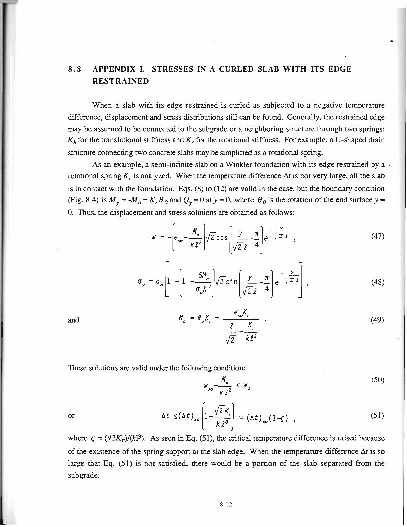
8.8 APPENDIX I. STRESSES IN A CURLED SLAB WITH ITS EDGE RESTRAINED

When a slab with its edge restrained is curled as subjected to a negative temperature

difference, displacement and stress dismbutions still can be found. Generally, the restrained edge

may be assumed to be connected to the subgrade or a neighboring structure through two springs: Kh for the translational stiffness and Kr for the rotational stiffness. For example, a U-shaped drain

structure connecting two concrete slabs may be simplified as a rotational spring.

As an example, a semi-infinite slab on a Winkler foundation with its edge restrained by a rotational spring K, is analyzed. When the temperature difference At is not very large, all the slab

is in contact with the foundation. Eqs. (8) to (12) are valid in the case, but the boundary condition (Fig. 8.4) is My = -M, = Kr 8, and Qy = 0 at y = 0, where Go is the rotation of the end surface y =

0. Thus, the displacement and stress solutions are obtained as follows:

and

These solutions are valid under the following condition:

where 5 = (42~,)l(kl3). As seen in Eq. (51), the critical temperature difference is raised because

of the existence of the spring support at the slab edge. When the temperature difference At is so large that Eq. (51) is not satisfied, there would be a portion of the slab separated from the

sub grade.

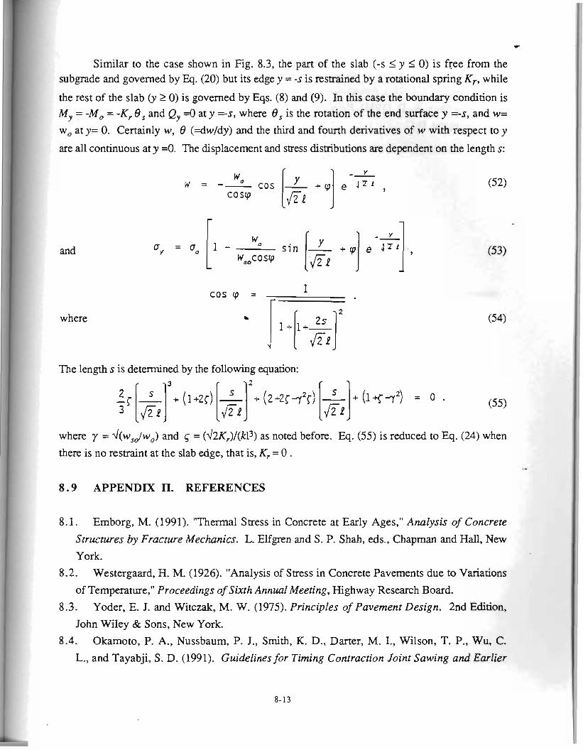
Similar to the case shown in Fig. 8.3, the part of the slab (-s I y I 0) is free from the subgrade and governed by Eq. (20) but its edge y = -s is restrained by a rotational spring Kr, while

the rest of the slab 6 2 0) is governed by Eqs. (8) and (9). In this case the boundary condition is My = -Mo = -K, 8, and Qy =O at y =-s, where 8, is the rotation of the end surface y =-s, and w=

wo at y= 0. Certainly w, 8 (=dw/dy) and the third and fourth derivatives of w with respect to y

are all continuous at y 4. The displacement and stress distributions are dependent on the length s:

and

where

cos cp = 1 r

The length s is determined by the following equation:

where y = d(wsdwo) and 5 = ( J X ~ ( k l 3 ) as noted before. Eq. (55) is reduced to Eq. (24) when

there is no restraint at the slab edge, that is, K, = 0 . .-

8 .9 APPENDIX 11. REFERENCES

8.1. Emborg, M. (1991). "Thermal Stress in Concrete at Early Ages," Analysis of Concrete

Structures by Fracture Mechanics. L. Elfgren and S. P. Shah, eds., Chapman and Hall, New

York.

8.2. Westergaard, H. M. (1926). "Analysis of Stress in Concrete Pavements due to Variations

of Temperature," Proceedings of Sixth Annual Meeting, Highway Research Board.

8.3. Yoder, E. J. and Witczak, M. W. (1975). Principles of Pavement Design. 2nd Edition,

John Wiley & Sons, New York.

8.4. Okamoto, P. A., Nussbaum, P. J., Smith, K. D., Darter, M. I., Wilson, T. P., Wu, C.

L., and Tayabji, S. D. (1991). Guidelines for Timing Contraction Joint Sawing and Earlier

*

Loading for Concrete Pavements, Report No. FHWA-RD-91-070, Federal Highway Administration, McLean, Virginia.

8 -5 . Scott, R. F. (198 1). Foundation Analysis. Prentice-Hall, Eaglewood Cliffs, New Jersey.

8.6. Bradbury, R. D. (1938), Reinforced Concrete Pavement, Wire Reinforcement Institute,

Washington, D.C.

-1uaura~~d jo a3q.m~ do1 ayl IE uop3arlp A a q u~ s s a s = 5 pue Suaua~td ayl jo a x p s do1 a q le uop3arlp x a q ssaas = - fuopxqp A ayl y ssass acsual u x n t q x m =D

fOpR3 S,UOSS!Od = ('l

fmarua~ed ayl 30 a3qms do1 aq1 pue a q . ~ n s uronoq a q uaamaq a3ua.xaj~q xwwadwn = IV

$ u a p g m uoy-edxa @uuaq = w fuop~arlp z a q y 1uauxa3t1dsp = M

tiuauxa~ed a q jo uoyas-ssm aql uo a q mays = a fuopepunoj atp rlq uop3mi = b

3uarua~vd arq jo uop3as-ssm a q uo luaurow =

f s s a g s aApep aql jo snpm = 3 lo 1

!ssaujms puopao~ = '2

tssaujj!ls puopelsm = qx

tsnppow uopepunoj = ;r tqdap maura~ed = y

tsn~tlpour s ,%uno~ = 3

:sa%d snl, ul pasn aJe s1oquAs %u~molloj a u

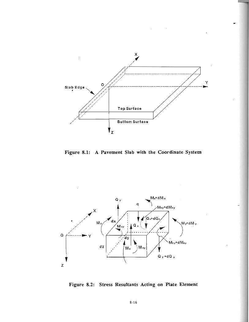
Figure 8.1: A Pavement Slab with the Coordinate System

Figure 8.2: Stress Resultants Acting on Plate Element

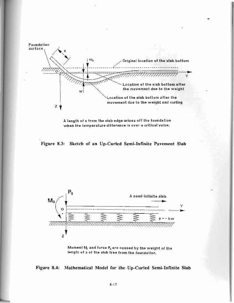
Foundation surface, ,,&

Original location o f the slab bo t tom

Locat ion o f the slab bo t tom a f t e r

I the movement due t o the we ight

\ ~ o c a t i o n o f the s lab bo t tom af te r the movement due t o the we igh t and curling

A length o f s f rom the slab edge arises o f f the foundation when the temperature dif ference i s over a cr i t ica l value.

Figure 8.3: Sketch of an Up-Curled Semi-Infinite Pavement Slab

Moil" A semi-infinite slab

+ Y

0 ................................................................. L- -.-.-. w

Moment FJ1 and force Po are caused b y the we ight o f the length of s o f the slab f ree f rom the foundation.

Figure 8.4: Mathematical Model for the Up-Curled Semi-Infinite Slab

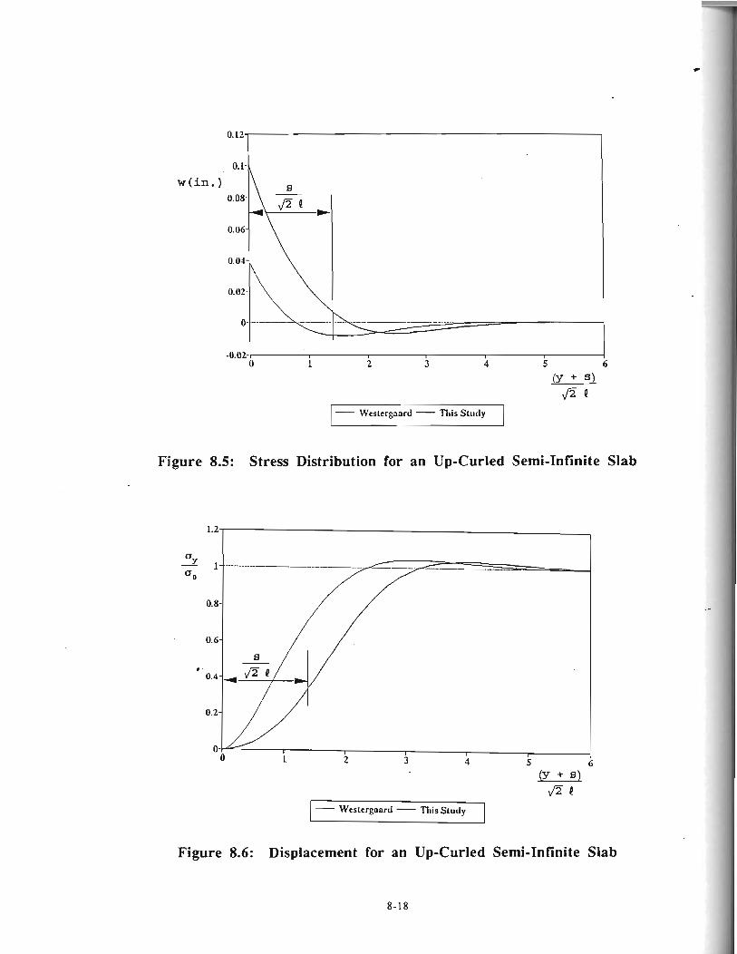
w (in. )

- Westergnard - n ~ i s Slucly

Figure 8.5: Stress Distribution for an Up-Curled Semi-Infinite Slab

- Weslcrgaard - n ~ i s Study

Figure 8.6: Displacement for an Up-Curled Semi-Infinite Slab

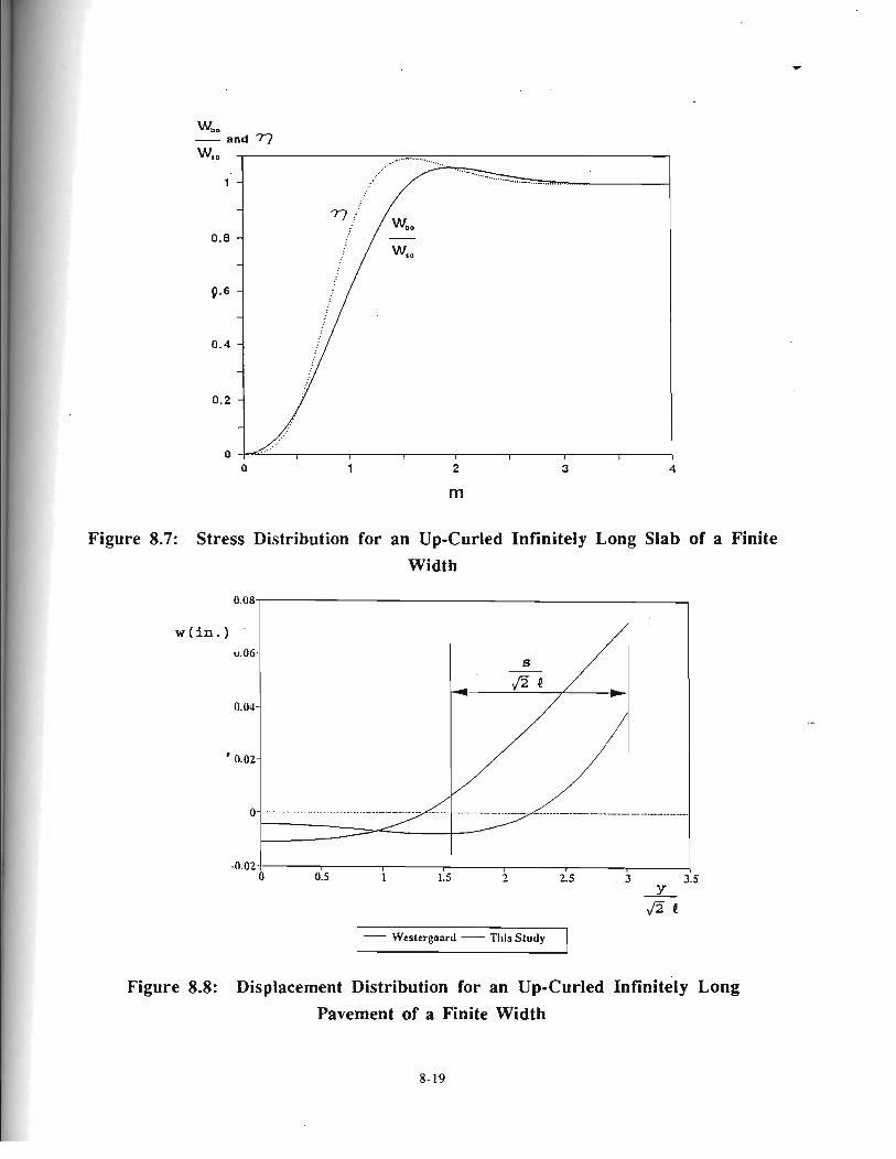
w,, - and 7 wso

1

Figure 8.7: Stress Distribution for an Up-Curled Infinitely Long Slab of a Finite Width

I - Westergand - This Study I

Figure 8.8: Displacement Distribution for an Up-Curled ~nfinitely Long Pavement of a Finite Width

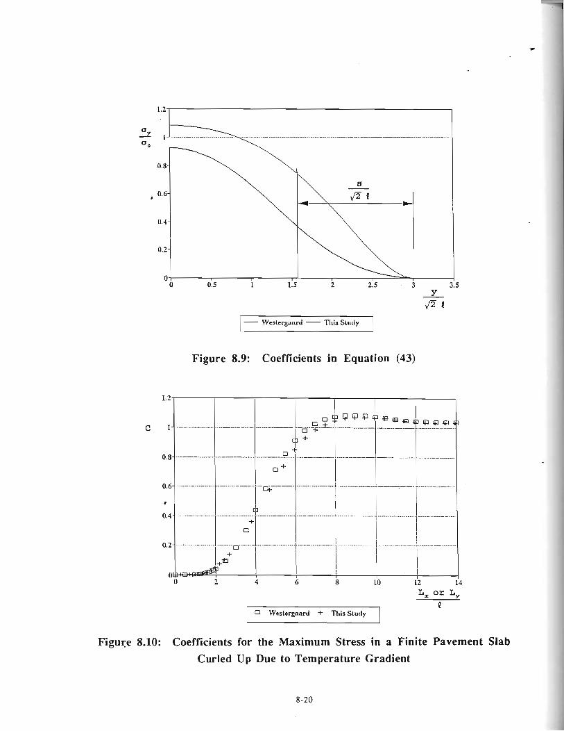
- Wesiergunrd - Tliis Study

Figure 8.9: Coefficients in Equation (43)

0 Wesiergnanl + T h i s Study

Figure 8.10: Coefficients for the Maximum Stress in a Finite Pavement Slab Curled Up Due to Temperature Gradient

CHAPTER 9

TWO-DIMENSIONAL ANALYSIS OF CRC PAVEMENT AT EARLY AGES

A two-dimensional finite element (FE) method is presented for the purpose of studying the

effects of concrete properties, steel reinforcement and environmental parameters on the early-aged

behavior of continuously reinforced concrete (CRC) pavements. The numerical procedure consists

of two parts, one related to moisture movement in the concrete and the other part related to the

concrete stress-strain analysis. The first stage predicts shrinkage strains developed due to moisture

loss from the concrete. It uses the semi-discrete method of nonlinear finite element analysis to

predict the moisture distribution in concrete as a function of time. This model is verified with

theoretical and experimental results available in the literature. An existing finite element model

previously developed for the analysis of moisture movement in subgrade soils [9.1] is modified

and adapted for analysis for concrete materials.

Shrinkage strains predicted in the first stage and the thermal strains imposed due to

variations in ambient temperature are used as input for the second stage of the analysis. This stage

predicts stress distribution with respect to the concrete creep of the pavement after initial

development of the crack pattern. The twodimensional CRC pavement analysis is simplified for

the finite element method based on plane strain assumptions (Figure 9.1) in which the bond slip is

modeled at the interface of concrete and steel. Analysis of the internal resmint is performed for

predicting subsequent concrete pavement stresses due to environmental effects. A finite element

code has been specifically developed for the stress analysis.

Previous analysis of CRC pavement [9.2, 9-33 behavior is one-dimensional in that the .-

stresses and strains vary in only one dimension or direction (i.e. along the longitudinal axis).

Therefore, the objective of this work is to develop a framework for the study of the various factors

affecting the crack formation in CRC pavement at an early age on a two-dimensional basis.

Development of the framework consists of the identification of the important models and

components of the analysis and how they may work together in the two-dimensional analysis of

CRC pavement. The cracks in CRC pavement are due to tensile stresses which develop in the

concrete pavement that exceed the tensile strength of concrete. The ambient climatic conditions and

structural configuration of the pavement are the primary causes for the development of tensile

stresses in the CRC pavement. In this report, the development of stresses will be characterized

with respect to shrinkage and temperature variations not only in the longitudinal direction but also

vertically through the slab thickness. Two different finite element models are implemented for the

t

analysis; one for the computation of shrinkage strains and the other for the stress analysis due to

shrinkage and thermal strains, respectively. This, comparatively speaking, is a step beyond

previous research efforts to characterize stresses in CRC pavement.

Bazant's equation 19-43 of non-linear diffusion theory is used for the finite element model

for shrinkage strains because of its inherent dependence upon material properties and its

applicability to twodimensional analysis. The code for this analysis is a modified version of a

model which predicts moisture movement in soils with respect to time. The other finite element

model is specially developed for the stress analysis which uses eight-noded isoparametric quadratic

elements and two noded spring elements for modeling bond between the concrete and the steel.

The predicted tensile stresses in the concrete by the model analysis are verified with the Vetter

model 19.51 based on a uniform distribution with depth of drying shrinkage. Various factors

affecting the tensile stress distribution in concrete are studied independently. The material .

properties of the concrete and steel are assumed to be linear and elastic.

Initial crack formation in reinforced concrete prior to complete curing is assumed to be due

to thermal and drying shrinkage as mentioned previously. Subsequent temperature drop and drying

shrinkage causes volumetric change in CRC pavement, which may be restrained by the steel

reinforcement. If the concrete is free to move then it will not experience any stress (be it tensile or

compressive), but if it is restrained fully or partially then stresses are developed in concrete. This

process is illustrated in Figures 9.2.1 and 9.2.2. If the tensile stress exceeds the tensile strength of

concrete then the concrete cracks. The strength is low in early-aged concrete. Since the hiffusivity

of moisture is very high during this period, shrinkage strains play a dominant role in both the initial

and subsequent cracking. The following mathematical models are developed for estimating the

shrinkage strains. Their effect is combined with that of thermal strains to predict a final stress state

for reinforced concrete.

9.1 THE STRESS MODEL

Finite element (FE) stress analysis is performed for imposed strains on early aged concrete.

The increase of strength and elasticity of concrete with age is accounted for in the analysis.

Typically, the increase in strength of concrete at an early age (i.e, within first seven days) is very

high. A typical example of the change of concrete strength with time 't' is illustrated in Figure 9.2. Similarly, the change of modulus of elasticity at any given time 't' is shown in Figure 9.3. Following are the empirical relations which represent these two curves [9.6]:

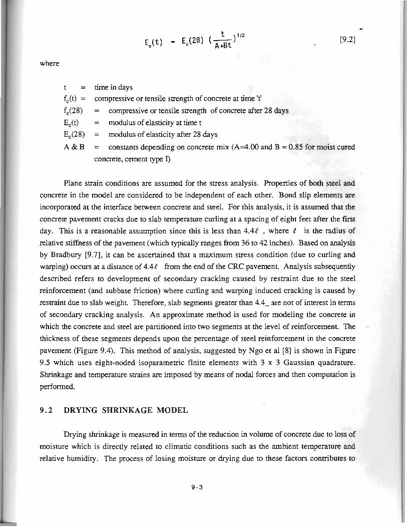
where

t = time in days

fc(t) = compressive or tensile strength of concrete at time 't'

fc(28) = compressive or tensile strength of concrete after 28 days

Ec(t) = modulus of elasticity at time t

Ec(28) = modulus of elasticity after 28 days

A & B = constants depending on concrete mix (A=4.00 and B = 0.85 for moist cured

concrete, cement type I)

Plane strain conditions are assumed for the stress analysis. Properties of both steel and

concrete in the model are considered to be independent of each other. Bond slip elements are

incorporated at the interface between concrete and steel. For this analysis, it is assumed that the

concrete pavement cracks due to slab temperature curling at a spacing of eight feet after the first day. This is a reasonable assumption since this is less than 4.41 , where 1 is the radius of

relative stiffness of the pavement (which typically ranges from 36 to 42 inches). Based on analysis

by Bradbury [9.7], it can be ascertained that a maximum stress condition (due to curling and

warping) occurs at a distance of 4.41 fiom the end of the CRC pavement. Analysis subsequently

described refers to development of secondary cracking caused by restraint due to the steel

reinforcement (and subbase friction) where curling and warping induced cracking is caused by

restraint due to slab weight Therefore, slab segments greater than 4.4- are not of interest in terns

of secondary cracking analysis. An approximate method is used for modeling the concrete in

which the concrete and steel are partitioned into two segments at the level of reinforcement. The - -

thickness of these segments depends upon the percentage of steel reinforcement in the concrete

pavement (Figure 9.4). This method of analysis, suggested by Ngo et a1 [8] is shown in Figure

9.5 which uses eight-noded isopararnemc finite elements with 3 x 3 Gaussian quadrature.

Shrinkage and temperature strains are imposed by means of nodal forces and then computation is

performed.

9.2 DRYING SHRINKAGE MODEL

Drying shrinkage is measured in terms of the reduction in volume of concrete due to loss of

moisture which is directly related to climatic conditions such as the ambient temperature and

relative humidity. The process of losing moisture or drying due to these factors conmbutes to

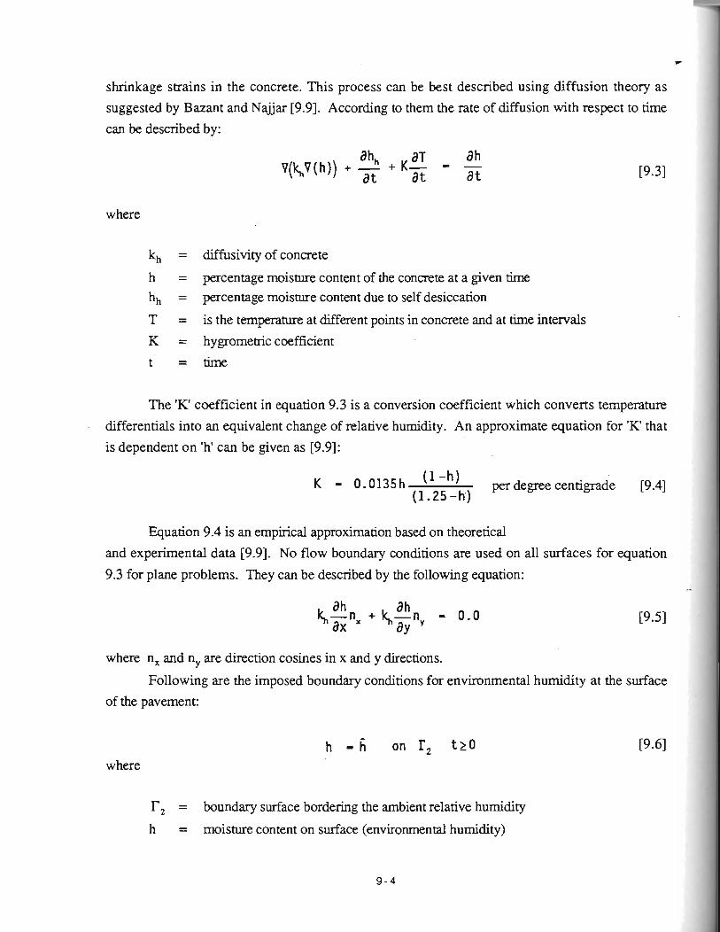
shrinkage strains in the concrete. This process can be best described using diffusion theory as

suggested by Bazant and Najjar 19.91. According to them the rate of diffusion with respect to time

can be described by:

where I

kh = diffusivity of concrete

h = percentage moisture content of the concrete at a given time h, = percentage moisture content due to self desiccation

T = is the temperature at different points in concrete and at time intervals

K = hygrometric coefficient

t = time

The 'R coefficient in equation 9.3 is a conversion coefficient which converts temperature

differentials into an equivalent change of relative humidity. An approximate equation for 'K' that

is dependent on 'h' can be given as [9.9]:

K - 0.0135h (1 -h ) per degree centigrade 19.41 (1 .25 -h )

I Equation 9.4 is an empirical approximation based on theoretical

and experimental data [9.9]. No flow boundary conditions are used on all surfaces for equation I

9.3 for plane problems. They can be described by the following equation:

where n, and ny are direction cosines in x and y directions.

Following are the imposed boundary conditions for environmental humidity at the surface of the pavement:

where

r, = boundary surface bordering the ambient relative humidity

h = moisture content on surface (environmental humidity)

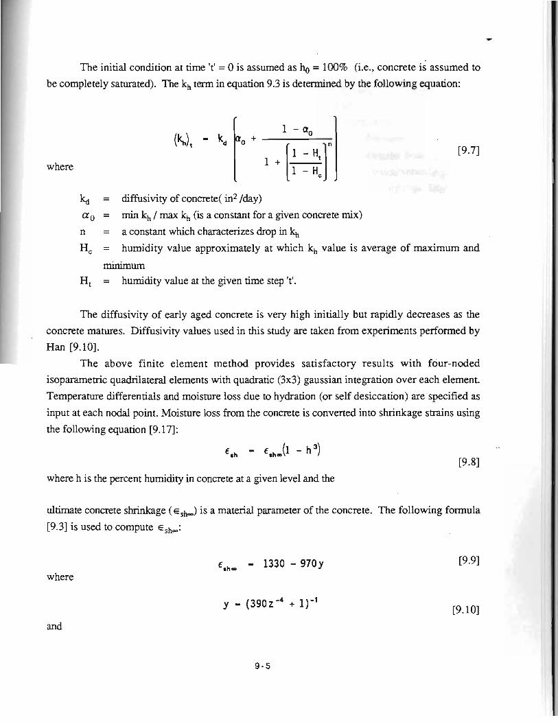
The initial condition at time 't' = 0 is assumed as = 100% (i.e., concrete i i assumed to

be completely saturated). The kh tenn in equation 9.3 is determined by the following equation:

f

(khIt - kd a0 +

where <

k, = diffisivity of concrete( in2 /day)

a,, = min kh / max lk (is a constant for a given concrete mix)

n = a constant which characterizes drop in lk H, = humidity value approximately at which kh value is average of maximum and

minimum

H, = humidity value at the given time step 't'.

The diffusivity of early aged concrete is very high initially but rapidly decreases as the

concrete matures. Diffusivity values used in this study are taken from experiments performed by Han [9.10].

The above finite element method provides satisfactory results with four-noded

isoparametric quadrilateral elements with quadratic (3x3) gaussian integration over each element.

Temperature differentials and moisture loss due to hydration (or self desiccation) are specified as

input at each nodal point. Moisture loss from the concrete is converted into shrinkage strains using

the following equation [9.17]:

'sh - 'she (I - h ')

where h is the percent humidity in concrete at a given level and the

ultimate concrete shrinkage (E,~,.) is a material parameter of the concrete. The following formula

[9.3] is used to compute E,~.,,,:

where

and

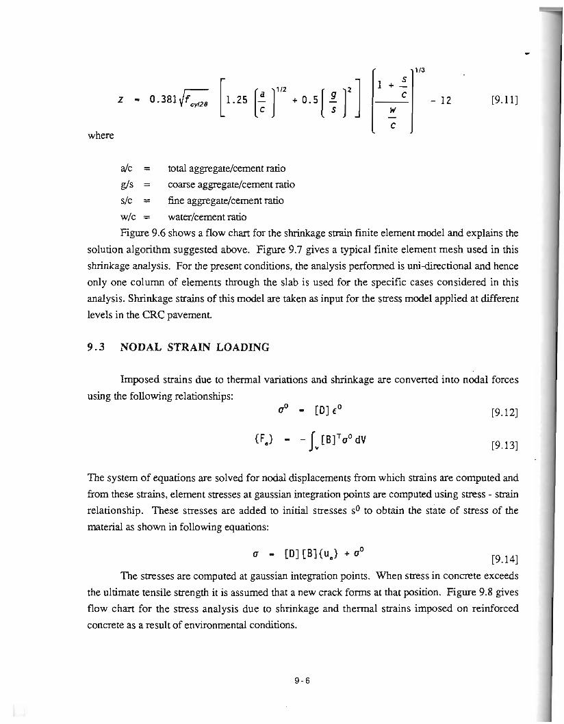
where

a/c = total aggregatelcement ratio g/s = coarse aggregate/cement ratio

SIC = fine aggregatelcement ratio

w/c = water/cement ratio

Figure 9.6 shows a flow chart for the shrinkage strain finite element model and explains the

solution algorithm suggested above. Figure 9.7 gives a typical finite element mesh used in this

shrinkage analysis. For the present conditions, the analysis performed is uni-directional and hence

only one column of elements through the slab is used for the specific cases considered in this

analysis. Shrinkage strains of this model are taken as input for the stress model applied at different

levels in the CRC pavement.

9.3 NODAL STRAIN LOADING

Imposed strains due to thermal variations and shrinkage are converted into nodal forces

using the following relationships: UO - [ D ] c0

The system of equations are solved for nodal displacements from which strains are computed and

from these strains, element stresses at gaussian integration points are computed using stress - strain

relationship. These stresses are added to initial stresses so to obtain the state of stress of the

material as shown in following equations:

The stresses are computed at gaussian integration points. When s a s s in concrete exceeds

the ultimate tensile strength it is assumed that a new crack forms at that position. Figure 9.8 gives

flow chart for the stress analysis due to shrinkage and thermal strains imposed on reinforced

concrete as a result of environmental conditions.

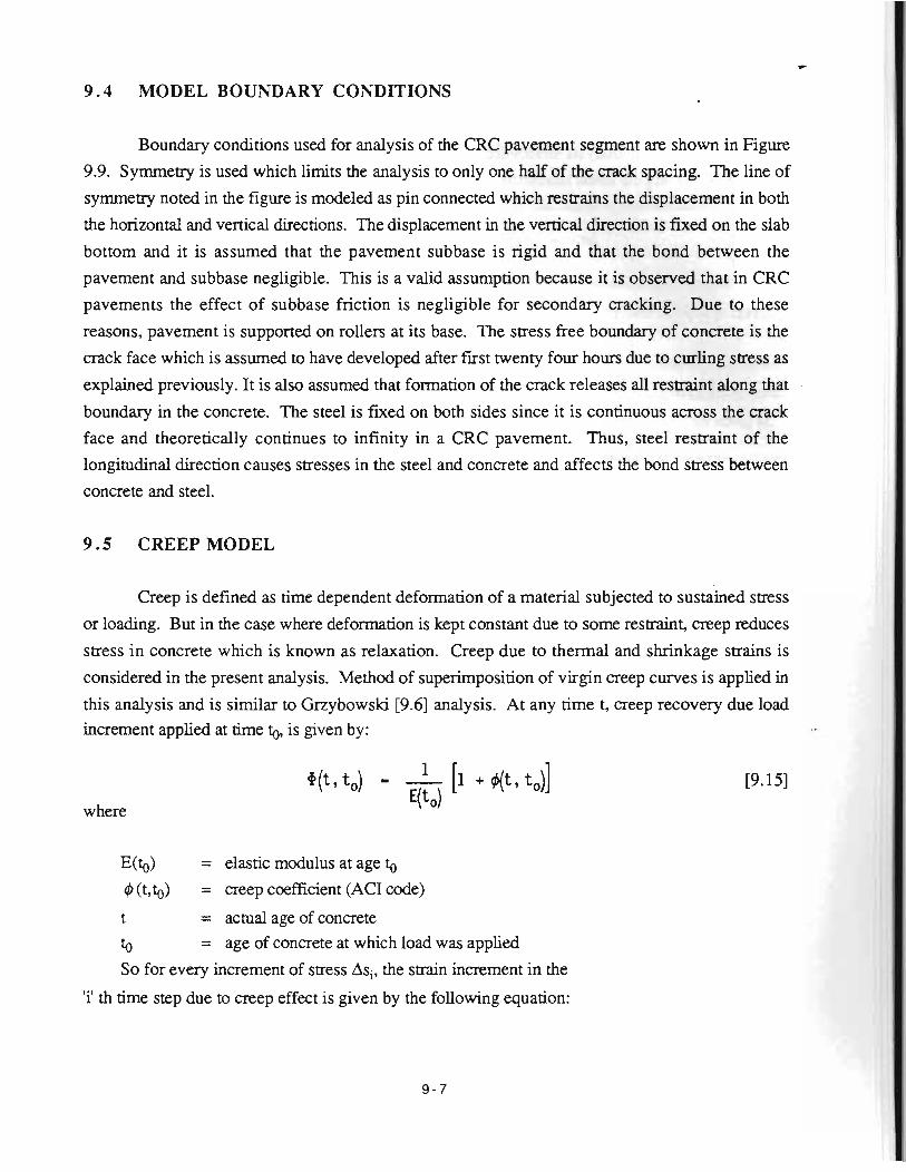
9 .4 MODEL BOUNDARY CONDITIONS

Boundary conditions used for analysis of the CRC pavement segment are shown in Figure

9.9. Symmetry is used which limits the analysis to only one half of the crack spacing. The line of

symmetry noted in the figure is modeled as pin connected which restrains the displacement in both

the horizontal and vertical directions. The displacement in the vertical direction is fixed on the slab

bottom and it is assumed that the pavement subbase is rigid and that the bond between the

pavement and subbase negligible. This is a valid assumption because it is observed that in CRC

pavements the effect of subbase friction is negligible for secondary cracking. Due to these

reasons, pavement is supported on rollers at its base. The stress free boundary of concrete is the

crack face which is assumed to have developed after first twenty four hours due to curling stress as

explained previously. It is also assumed that foxmation of the crack releases all restraint along that

boundary in the concrete. The steel is fixed on both sides since it is continuous across the crack face and theoretically continues to infinity in a CRC pavement. Thus, steel restraint of the

longitudinal direction causes stresses in the steel and concrete and affects the bond stress between

concrete and steel.

9.5 CREEP MODEL

Creep is defined as time dependent deformation of a material subjected to sustained stress

or loading. But in the case where deformation is kept constant due to some restraint, creep reduces

stress in concrete which is known as relaxation. Creep due to thermal and shrinkage strains is

considered in the present analysis. Method of superimposition of virgin creep curves is applied in

this analysis and is similar to Grzybowski [9.6] analysis. At any time t, creep recovery due load increment applied at time to, is given by:

where

E(to) = elastic modulus at age to 4 (t,@ = creep coefficient (ACI code)

t = actual age of concrete

to = age of concrete at which load was applied So for every increment of stress Asi, the strain increment in the

'i' th time step due to creep effect is given by the following equation:

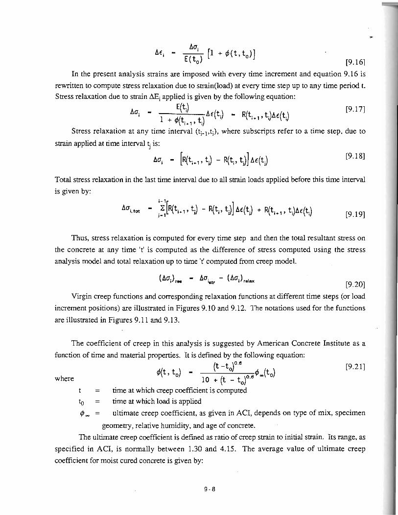
In the present analysis strains are imposed with every time increment and equation 9.16 is

rewritten to compute stress relaxation due to strain(1oad) at every time step up to any time period t. Stress relaxation due to strain AEi applied is given by the following equation:

Stress relaxation at any time interval (ti-*,ti), where subscripts refer to a time step, due to I

I

strain applied at time interval tj is: I

Total stress relaxation in the last time interval due to all strain loads applied before this time interval is given by:

i-lr 1

Thus, stress relaxation is computed for every time step and then the total resultant stress on the concrete at any time 't' is computed as the difference of stress computed using the stress

analysis model and total relaxation up to time 't' computed from creep model.

Virgin creep functions and corresponding relaxation functions at different time steps (or load

increment positions) are illustrated in Figures 9.10 and 9.12. The notations used for the functions

are illustrated in Figures 9.1 1 and 9.13.

The coefficient of creep in this analysis is suggested by American Concrete Institute as a

function of time and material properties. It is defined by the following equation:

where

t = time at which creep coefficient is computed to = time at which load is applied

6, = ultimate creep coefficient, as given in ACI, depends on type of mix, specimen

geometry, relative humidity, and age of concrete.

The ultimate creep coefficient is defined as ratio of creep strain to initial strain. Its range, as I

specified in ACI, is normally between 1.30 and 4.15. The average value of ultimate creep

coefficient for moist cured concrete is given by:

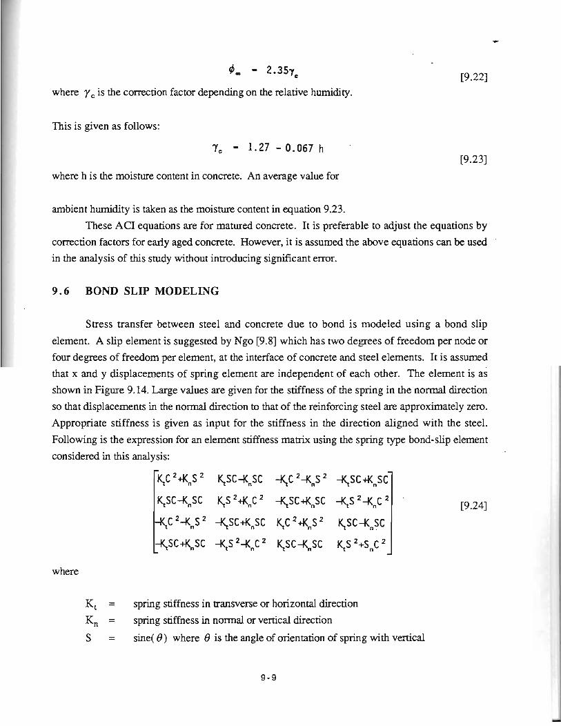
6, - 2.357,

where y, is the correction factor depending on the relative humidity.

This is given as follows:

Y - 1.27 - 0.067 h

where h is the moisture content in concrete. An average value for

ambient humidity is taken as the moisture content in equation 9.23. These ACI equations are for matured concrete. It is preferable to adjust the equations by

correction factors for early aged concrete. However, it is assumed the above equations can be used

in the analysis of this study without introducing significant error.

9 . 6 BOND SLIP MODELING

Stress transfer between steel and concrete due to bond is modeled using a bond slip

element. A slip element is suggested by Ngo [9.8] which has two degrees of freedom per node or

four degrees of freedom per element, at the interface of concrete and steel elements. It is assumed . .

that x and y displacements of spring element are independent of each other. The element is as

shown in Figure 9.14. Large values are given for the stiffness of the spring in the normal direction

so that displacements in the normal direction to that of the reinforcing steel are approximately zero.

Appropriate stiffness is given as input for the stiffness in the direction aligned with the steel.

Following is the expression for an element stiffness matrix using the spring type bond-slip element

considered in this analysis:

where

Kt = spring stiffness in transverse or horizontal direction

K,., = spring stiffness in normal or vertical direction

S = sine( 8) where 8 is the angle of orientation of spring with vertical

*

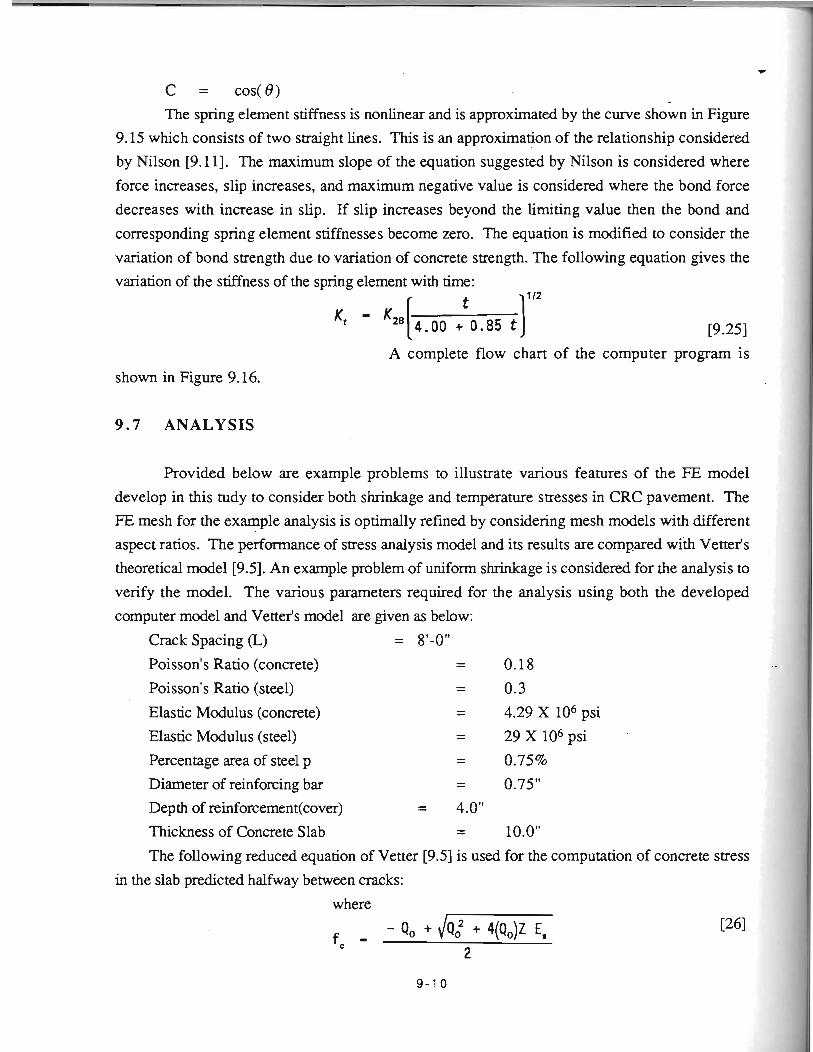
C = cos(0) The spring element stiffness is nonlinear and is approximated by the curve shown in Figure

9.15 which consists of two straight lines. This is an approximation of the relationship considered

by Nilson [9.11]. The maximum slope of the equation suggested by Nilson is considered where

force increases, slip increases, and maximum negative value is considered where the bond force

decreases with increase in slip. If slip increases beyond the limiting value then the bond and

corresponding spring element stiffnesses become zero. The equation is modified to consider the

variation of bond strength due to variation of concrete strength. The following equation gives the

variation of the stiffness of the spring element with time:

A complete flow chart of the computer program is

shown in Figure 9.16. 1

9.7 ANALYSIS

Provided below are example problems to illustrate various features of the FE model

develop in this tudy to consider both shrinkage and temperature stresses in CRC pavement. The I

FE mesh for the example analysis is optimally refined by considering mesh models with different aspect ratios. The performance of stress analysis model and its results are compared with Vetteis

theoretical model [9.5]. An example problem of uniform shrinkage is considered for the analysis to

verify the model. The various parameters required for the analysis using both the developed

computer model and Vetter's model are given as below: 1 I

Crack Spacing (L) = 81-0"

Poisson's Ratio (concrete) - - 0.18 .-

Poisson's Ratio (steel) - - 0.3

Elastic Modulus (concrete) = 4.29X106psi

Elastic Modulus (steel) - - 29 X lo6 psi

Percentage area of steel p - - 0.75%

Diameter of reinforcing bar - - 0.75"

Depth of reinforcement(cover) = 4.0"

Thickness of Concrete Slab - - 10.0~ i The following reduced equation of Vetter [9.5] is used for the computation of concrete stress I

in the slab predicted halfway between cracks: ~ where

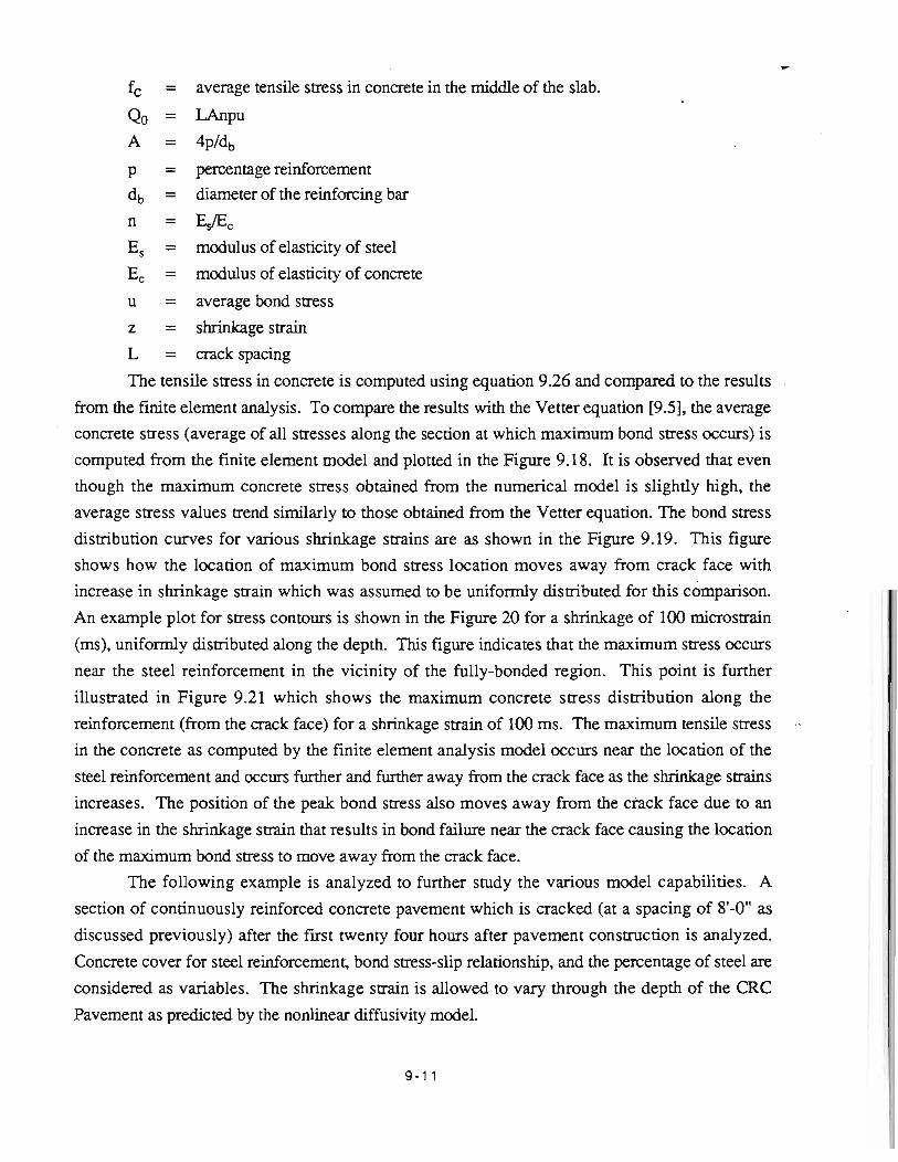
fc = average tensile stress in concrete in the middle of the slab.

Qo = LA"Pu A = 4p/db

p = percentage reinforcement db = diameter of the reinforcing bar

n = W C

E, = modulus of elasticity of steel

E, = modulus of elasticity of concrete

u = average bond stress

z = shrinkage strain

L = crack spacing

The tensile stress in concrete is computed using equation 9.26 and compared to the results

from the finite element analysis. To compare the results with the Vetter equation [9.5], the average

concrete stress (average of all stresses along the section at which maximum bond stress occurs) is

computed from the finite element model and plotted in the Figure 9.18. It is observed that even

though the maximum concrete stress obtained from the numerical model is slightly high, the

average stress values trend similarly to those obtained from the Vetter equation. The bond stress

distribution curves for various shrinkage strains are as shown in the Figure 9.19. This figure

shows how the location of maximum bond stress location moves away from crack face with

increase in shrinkage strain which was assumed to be uniformly dismbuted for this comparison.

An example plot for stress contours is shown in the Figure 20 for a shrinkage of 100 microstrain

(ms), uniformly distributed along the depth. This figure indicates that the maximum stress occurs near the steel reinforcement in the vicinity of the fully-bonded region. This point is further

illustrated in Figure 9.21 which shows the maximum concrete stress distribution along the

reinforcement (from the crack face) for a shrinkage strain of 100 ms. The maximum tensile stress .-

in the concrete as computed by the finite element analysis model occurs near the location of the

steel reinforcement and occurs further and further away from the crack face as the shrinkage strains

increases. The position of the peak bond stress also moves away from the crack face due to an

increase in the shrinkage strain that results in bond failure near the crack face causing the location

of the maximum bond stress to move away from the crack face.

The following example is analyzed to further study the various model capabilities. A

section of continuously reinforced concrete pavement which is cracked (at a spacing of 8'-0" as discussed previously) after the first twenty four hours after pavement construction is analyzed.

Concrete cover for steel reinforcement, bond stress-slip relationship, and the percentage of steel are considered as variables. The shrinkage strain is allowed to vary through the depth of the CRC

Pavement as predicted by the nonlinear diffusivity model.

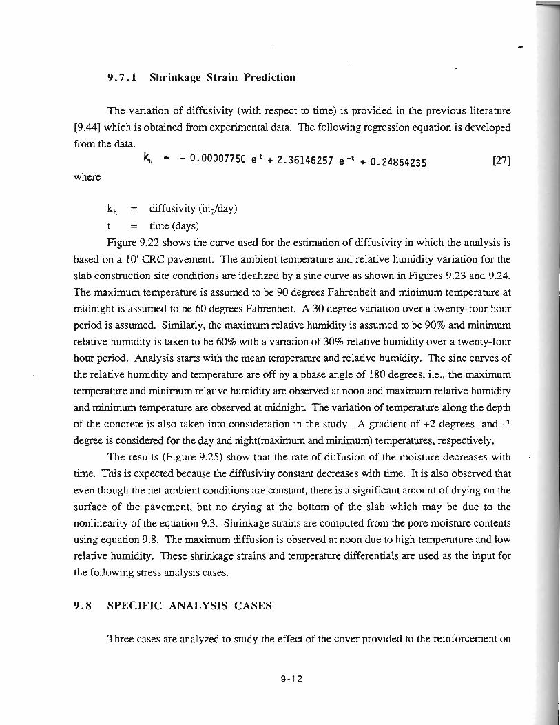
9.7 .1 Shrinkage Strain Prediction

The variation of diffusivity (with respect to time) is provided in the previous literature

[9.44] which is obtained from experimental data. The following regression equation is developed from the data.

k,, - - 0.00007750 e ' + 2.36146257 e-' + 0.24864235 1271

where

kh = diffusivity (in2/day)

t = time (days)

Figure 9.22 shows the curve used for the estimation of diffusivity in which the analysis is

based on a 10' CRC pavement. The ambient temperature and relative humidity variation for the

slab construction site conditions are idealized by a sine curve as shown in Figures 9.23 and 9.24.

The maximum temperature is assumed to be 90 degrees Fahrenheit and minimum temperature at

midnight is assumed to be 60 degrees Fahrenheit. A 30 degree variation over a twenty-four hour

period is assumed. Similarly, the maximum relative humidity is assumed to be 90% and minimum

relative humidity is taken to be 60% with a variation of 30% relative humidity over a twenty-four

hour period. Analysis starts with the mean temperature and relative humidity. The sine curves of the relative humidity and temperature are off by a phase angle of 180 degrees, i.e., the maximum

temperature and minimum relative humidity are observed at noon and maximum relative humidity

and minimum temperature are observed at midnight. The variation of ttmpmLNe along the depth

of the concrete is also taken into consideration in the study. A gradient of +2 degrees and -1

degree is considered for the day and night(maximurn and minimum) temperatures, respectively.

The results (Figure 9.25) show that the rate of diffusion of the moisture decreases with -

time. This is expected because the diffusivity constant decreases with time. It is also observed that

even though the net ambient conditions are constant, there is a significant amount of drying on the

surface of the pavement, but no w i n g at the bottom of the slab which may be due to the

nonlinearity of the equation 9.3. Shrinkage strains are computed from the pore moisture contents

using equation 9.8. The maximum diffusion is observed at noon due to high temperature and low

relative humidity. These shrinkage strains and temperature differentials are used as the input for

the following stress analysis cases.

9.8 SPECIFIC ANALYSIS CASES

Three cases are analyzed to study the effect of the cover provided to the reinforcement on

9-12

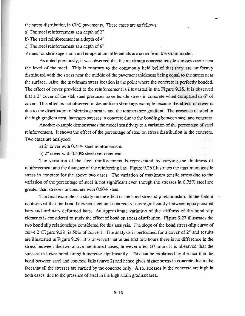
the stress distribution in CRC pavements. These cases are as.follows:

a) The steel reinforcement at a depth of 2"

b) The steel reinforcement at a depth of 4"

c) The steel reinforcement at a depth of 6" Values for shrinkage strain and temperature differentials are taken from the strain model.

As noted previously, it was observed that the maximum concrete tensile stresses occur near

the level of the steel. This is contrary to the commonly held belief that they are uniformly

distributed with the stress near the middle of the pavement thickness being equal to the stress near

the surface. Also, the maximum stress location is the point where the concrete is perfectly bonded.

The effect of cover provided to the reinforcement is illustrated in the Figure 9.25. It is observed

that a 2" cover of the slab steel produces more tensile stress in concrete when compared to 6" of

cover. This effect is not observed in the uniform shrinkage example because the effect of cover is

due to the distribution of shrinkage strains and the temperature gradient. The presence of steel in

the high gradient area, increases stresses in concrete due to the bonding between steel and concrete.

Another example demonstrates the model sensitivity to a variation of the percentage of steel

reinforcement. It shows the effect of the percentage of steel on stress distribution in the concrete.

Two cases are analyzed:

a) 2" cover with 0.75% steel reinforcement

b) 2" cover with 0.50% steel reinforcement

The variation of the steel reinforcement is represented by varying the thickness of

reinforcement and the diameter of the reinforcing bar. Figure 9.26 illustrates the maximum tensile

stress in concrete for the above two cases. The variation of maximum tensile stress due to the

variation of the percentage of steel is not significant even though the stresses in 0.75% steel are

greater than stresses in concrete with 0.50% steel.

The final example is a study on the effect of the bond stress-slip relationship. In the field it

is observed that the bond between steel and concrete varies significantly between epoxy-coated

bars and ordinary deformed bars. An approximate variation of the stiffness of the bond slip

elements is considered to study the effect of bond on stress distribution. Figure 9.27 illustrates the

two bond slip relationships considered for this analysis. The slope of the bond stress-slip curve of

curve 2 (Figure 9.28) is 50% of curve 1. The analysis is performed for a cover of 2" and results

are illustrated in Figure 9.29. It is observed that in the first few hours there is no difference in the

stress between the two above mentioned cases, however after 60 hours it is observed that the

stresses in lower bond strength increase significantly. This can be explained by the fact that the

bond between steel and concrete fails (curve 2) and hence gives higher stress in concrete due to the

fact that all the stresses are carried by the concrete only. Also, stresses in the concrete are high in

both cases, due to the presence of steel in the high strain gradient area.

*

The above four example problems describe the capabilities of the framework. Also the

effect of the ambient temperature and ambient humidity on the CRC pavements is illustrated for

various reinforcement covers and bond slip relationships.

9.9 SUMMARY

A procedural for numerical analysis framework is developed to determine shrinkage strains

and the corresponding tensile stresses in reinforced concrete slabs. Even though previous literature

addresses these problems, most models either do not consider the non-uniform distribution of

shrinkage strains nor the bond slip variation in the concrete. In this study, a framework is

developed to consider not only these effects, but how they vary with respect to ambient climatic

conditions in addition to creep relaxation.

Following are the conclusions anived from the analysis of example problems: a) Vetter's [9.5] equations may be applied for predicting the average tensile stress in the

middle of crack spacing; however, it is observed that due to the bond between steel and concrete,

maximum tensile stress in concrete is observed at the level of steel for pavements with 2" cover and

in the middle of crack spacing for 6" slab and is more than the average tensile stress. Hence, for

detailed stress analysis in the prediction of cracking, uniform shrinkage considered in Vetter's

equation may not be applicable.

b) The cover provided to the reinforcement may become a significant factor in pavement

design. Especially under field conditions, where the variation of temperature over a day is more

than what is assumed, that is 30' Fahrenheit over a twenty four hour period.

c) More detailed research should be performed toward determination

of the bond-slip relationship, because of its effect on stress distribution in concrete.

d) Non linear stress strain equations may have to be performed for the crack initiation and .-

propagation problems instead of elastic approach considered in the present analysis.

Further research needs to be performed in the determination of the bond stress-slip

relationship. Determination of bond characteristics between steel and concrete for different type of

steel bars such as plain, deformed or epoxy coated is significant for the prediction of actual stress

state of concrete. Although there are some experimental relationships for the determination of bond

stress for a given slip, they are mostly pull-out (steel bar embedded in concrete being pulled out

and then studying the strains developed in the bar and concrete) type of experiments, validity of

these models for the problems considered in this study should be studied further. Also the model

should be improved to consider different stiffness for spring elements along the reinforcement

because it was demonstrated that the bond stress-slip relationship varies along the reinforcement

[9.12]. The variation of bond stress-slip relationship with time should also be determined.

* Simplified assumption that this variation is similar to the variation of the modulus of concrete is

made in this study. There is no available evidence in the literature that this analysis is performed

for bond between concrete and steel, The analysis indicated a lack of sensitivity to the percentage

of reinforcement on concrete stress. This may have been due to the FE representation used for the

steel bar. It is recommended that further analysis of this effect be considered perhaps using a

different technique to represent the steel bar.

The model results should be verified with experimental results. Although the model is

verified for average stress in the concrete with Vetter's model, it should be verified in the actual

field conditions and hence suggested that some experiments are performed.

The model is limited to the prediction of maximum tensile stress. Hence for the study of

actual crack mechanism and its propagation, a crack tip element, should be included in the model.

This will allow the model to develop modified crack spacing and will be more realistic

approximation of the field conditions.

9.10 REFERENCES

D. A. Gay, "Development of a Predictive Model for Pavement Roughness on Expansive

Clay," Dissertation, Civil Engineering Department, Texas A&M University, August 1991.

M. Won, K. Hankins and B. F. McCullough, "Mechanistic Analysis of Continuously

Reinforced Concrete Pavements Considering Material Characteristics, Variability and

Fatigue," Center of Transportation Research, University of Texas at Austin, 1990.

R. L. Lytton, D. E. Pufahl, C. H. Michalak, H. S. Liang and B. J. Dempson, "An

Integrated Model of Climatic Effects on Pavements," Report No. FHWA-RD-90-033,

February 1990.

2. P. Ba-ant, "Constitutive Equation for Concrete Creep and Shrinkage Based on - Thermodynamics of Multiphase Systems," Materials and Structures (RILEM), Vol. 3, 1970,

p. 3-36.

C. P. Vetter, "Stresses in Reinforced Concrete Due to Volume .Changes," ASCE

Proceedings, Paper No. 1848, Feb. 1932.

M. Gnybowski and S. P. Shah, "Model to Predict Cracking in Fibre Reinforced

Concrete Due to Restrained Shrinkage," Magazine of Concrete Research, Vol. 41, No. 148,

Sept. 1989, p. 125-135.

R. D. Bradbury, "Reinforced Concrete Pavement," Wire Reinforcement Institute,

Washington, D. C., 1938.

D. Ngo and A. C. Scordelis, "Finite Element Analysis of Reinforced Concrete Beams,"

Title No. 64-14, ACI Journal, March 1967.

*

9.9. 2. P. Ba-ant and L. J. Najjar, "Drymg of Concrete 'as a Nonlinear Diffusion Problem,"

Cement and Concrete Research, Vol. 1, 1973, p. 461-73.

9.10. M. Y. Han and R. L. Lytton, "Permeability and Dimensional Change of Plain and

Polypropylene Fibre Concrete," Proposed to Journal of Engineering Materials, ASCE

(Private Collection, S. Kadiyala).

9.1 1. A. H. Nilson, "Nonlinear Analysis of Reinforced Concrete by the Finite Element," ACI

Journal, Title No. 65-55, Sept. 1968.

9.12. A. H. Nilson, "Internal Measurement of Bond Slip," Title No. 69-41, ACI Summary

Paper, ACI Journal, July 1972.

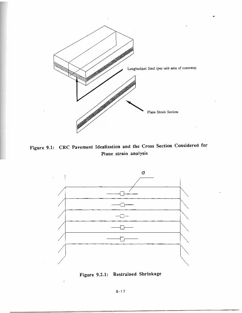
(per unit area of

Strain Section

concrete)

Figure 9.1: CRC Pavement Idealization and the Cross Section Considered for Plane strain analysis

Figure 9.2.1: Restrained Shrinkage

9-1 7

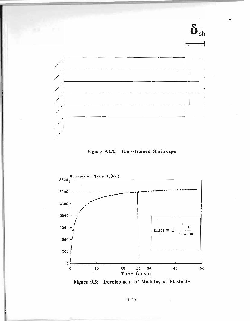
Figure 9.2.2: Unrestrained Shrinkage

Modulus of Elasticity(ksi) 3500 1 1

- - - - -

1

Ec(t) = Ec28 '---

1000 - ,I:-

500 -.

0 ' 1 I f I

0 10 20 28 30 40 5 0

Time (days)

Figure 9.3: Development of Modulus of Elasticity

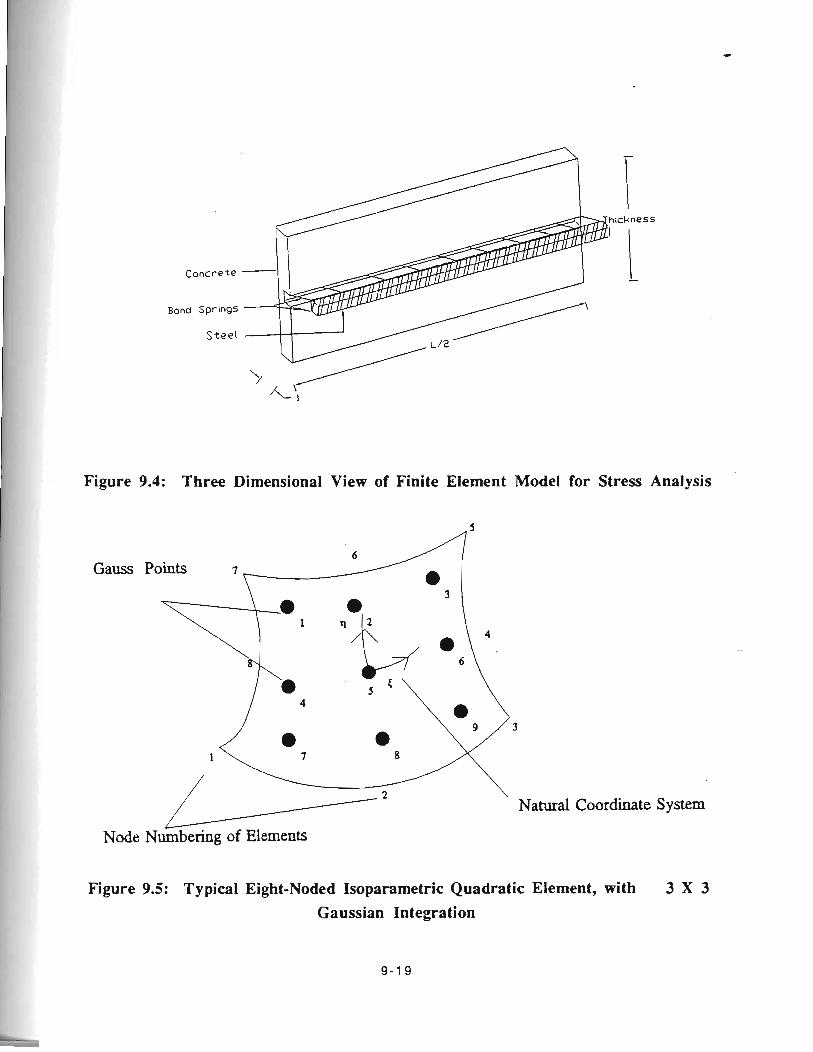
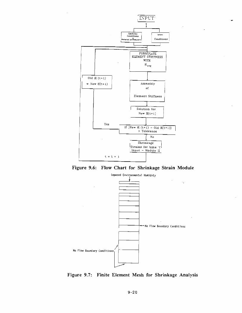
I ELEMENT STIFFNESS

= New H(t+l)

WITH

H avp

Assembly 47 1 Element Stiffness I

+ Solution for 1

I Yes / if (New H(t+!) - Old H(t+l))

> Tolerance

Strains for time 't'

Figure 9.6: Flow Chart for Shrinkage Strain Module Imposed Environmental Humidity

I

w +No Flow Boundary Conditions

Figure 9.7: Finite Element Mesh for Shrinkage Analysis

s!sL~euy ssaqg JOJ qsaw ~uarual3 a)!u!d pue suo!qpuo3 b~epunoa :g06 a ~ n % ! ~

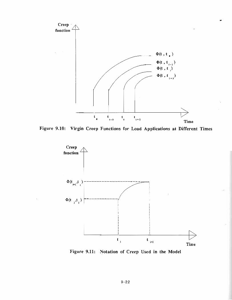
Creep .

function $

Figure 9.10: Virgin Creep Functions for Load Applications at Different Times

Creep .

function

Figure 9.11: Notation of Creep Used in the Model

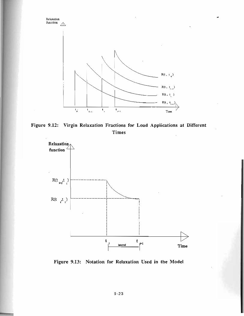
Relaxation function ~1

t

Figure 9.12: Virgin Relaxation Fractions for Load Applications at Different Times

Relaxation function

R(t **,t *) -------------.

R(t ') --------I--- \ I

r-------- -1

I I I I 1 I I I I I I I I I I I I I I I I I I I I I

t Time

Figure 9.13: Notation for Relaxation Used in the Model

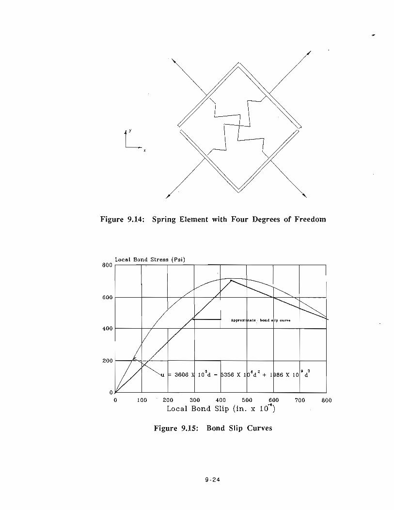
Figure 9.14: Spring Element with Four Degrees of Freedom

Local Bond Stress (Psi) 800

U

0 100 ' 200 300 400 500 600 700 800

Local Bond Slip (in. x lo*)

' Approdlnab.. bond s Ip ouno

= 3606 X load - 5356 X 13'd2 + 1386 X 10'd3

Figure 9.15: Bond Slip Curves

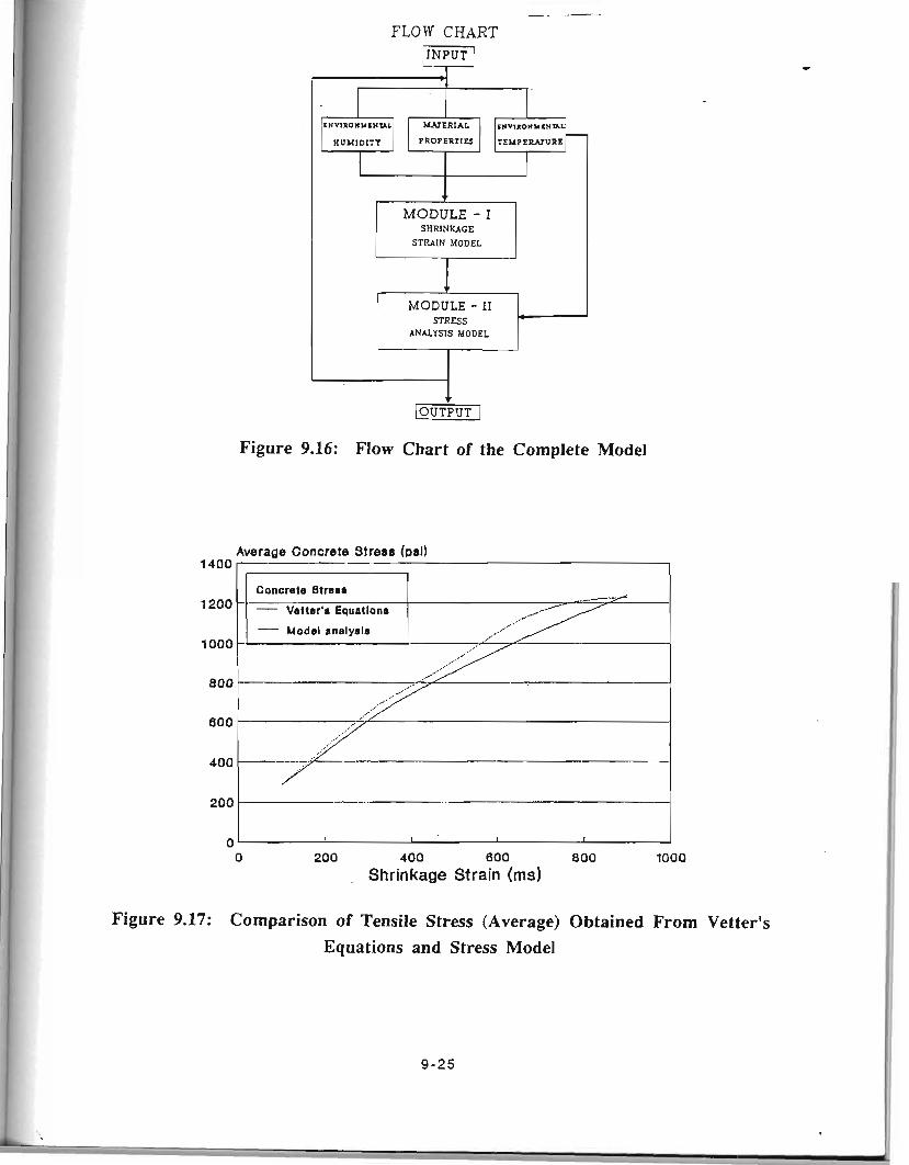
FLOW CHART INPUT

C

I '

~ ~ N V I E O N Y S N U L ).WERIAL E n v t ~ O N M s N u

HUMIDITY PROPERTIES TEMPEPA3URE

- t

MODULE - I SHRINKAGE

STRAIN MODEL

MODULE - 11

I ANALYSIS MODEL

Figure 9.16: Flow Chart of the Complete Model

Average Concrete Stress (psi) 1400

I I 1 Conoreta Itre88

Vetter'r Equatlonr ....

Model rnrlyala ,...' ...'/

0 1 I I I I I 0 200 400 600 800 1000

. Shrinkage Strain (ms)

Figure 9.17: Comparison of Tensile Stress (Average) Obtained From Vetter's Equations and Stress Model

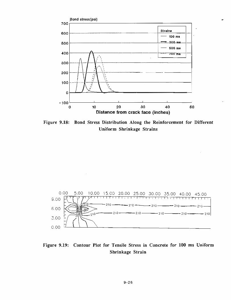
Bond stress(psi) 700

'

-100 0 10 20 30 40 6 0

Distance from crack face (inches)

Figure 9.18: Bond Stress Distribution Along the Reinforcement for Different Uniform Shrinkage Strains

Figure 9.19: Contour Plot for Tensile Stress in Concrete for 100 ms Uniform Shrinkage Strain

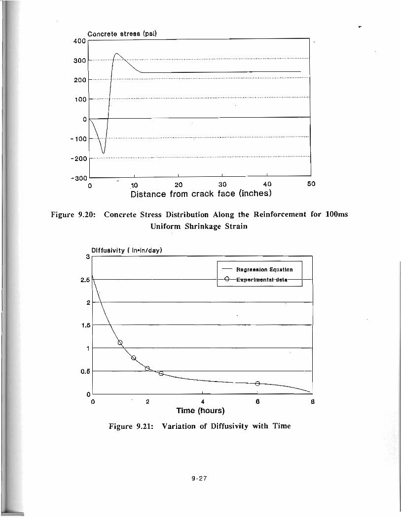
(saym!) age4 ~ 3 l e ~ 3 UJOJJ aDueJs!a 0s OP OE 02 OL - 0

I I I I OOE - ................................................................................................................................ 4 ooz-

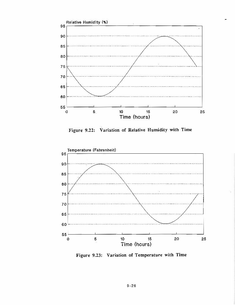
Relative Humidity (%) 96 1

I I I I I

0 5 10 15 20 25 Time (hours)

Figure 9.22: Variation of Relative Humidity with Time

Temperature (Fahrenheit) 96

55 I I I I I

0 5 10 15 20 2 5

Time (hours)

Figure 9.23: Variation of Temperature with Time

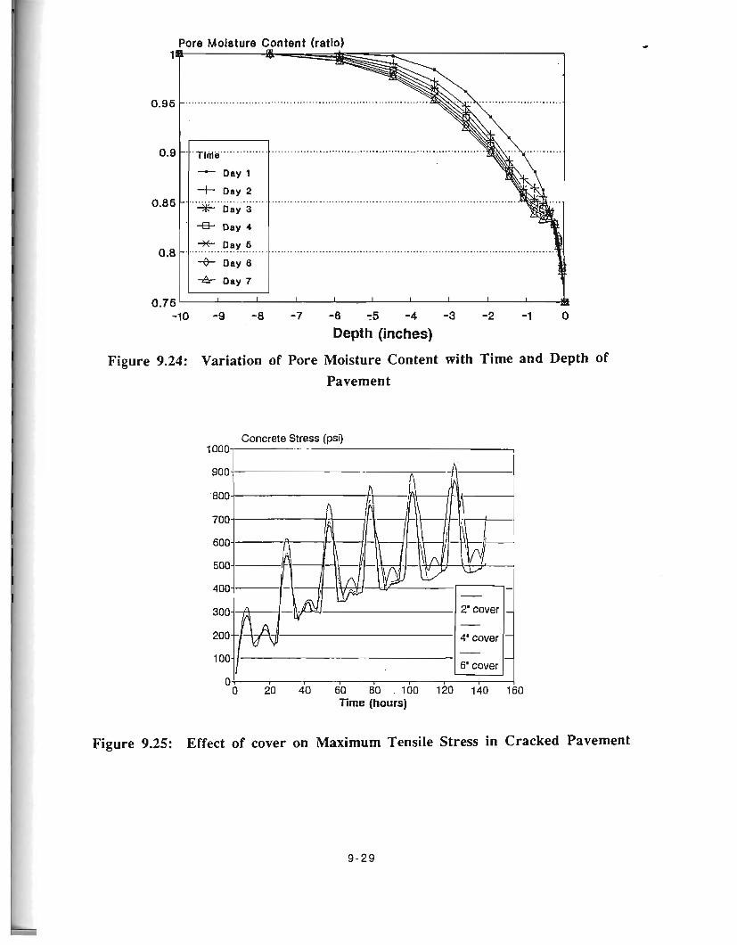
09C OPC 021 0 0 1 ' 08 09 OP 02 0 f0

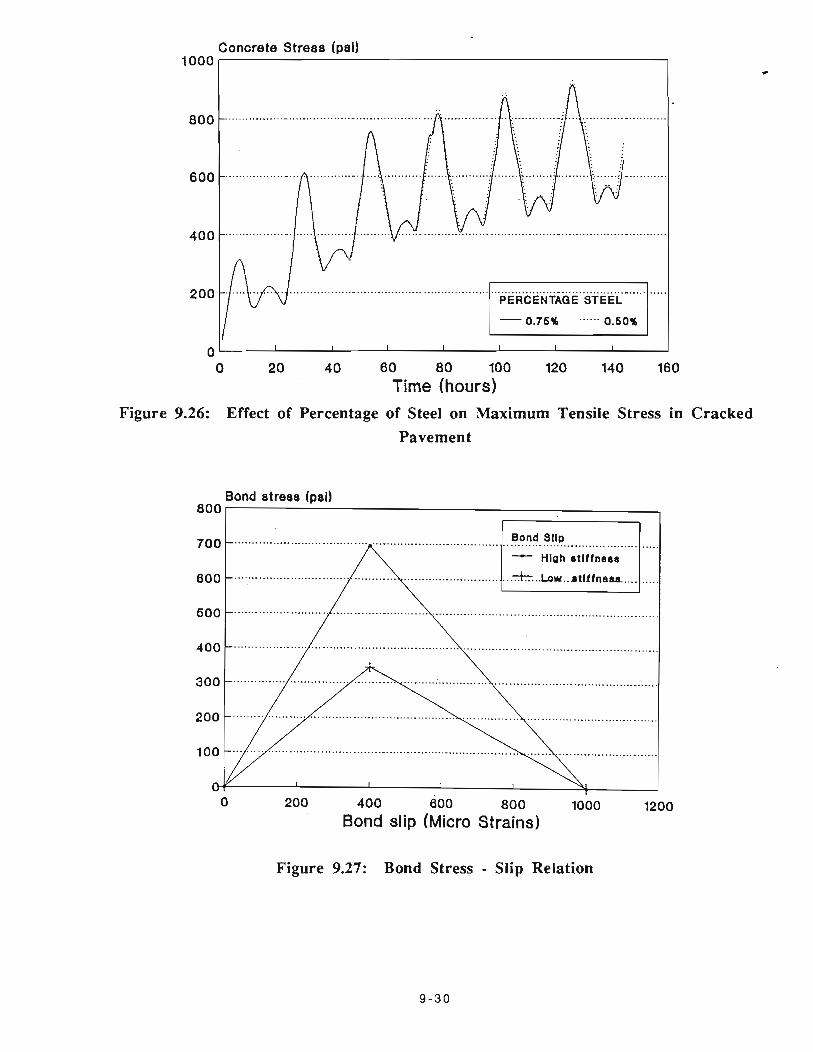
Concrete Stress (psi) 1000 1 1

PERCENTAGE STEEL

0.76% -""' 0.60%

u -

0 20 40 60 8 0 100 120 140 160 Time (hours)

Figure 9.26: Effect of Percentage of Steel on Maximum Tensile Stress in Pavement

Bond stre88 (psi) 800

r I

Hloh rtlttners .*... Low..ntIf Inem ..........

0 200 400 600 800 1000 1200 Bond slip (Micro Strains)

Cracked

Figure 9.27: Bond Stress - Slip Relation

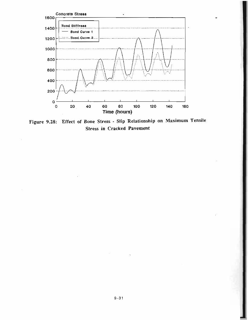
Concrete Stress I

Bond Stlflness

Bond Curve 1

0 I

I I I I I I I I 0 20 40 6 0 80 100 120 140 160

Time (hours)

Figure 9.28: Effect of Bone Stress - Slip Relationship on Maximum Tensile Stress in Cracked Pavement

CHAPTER 10

CONCLUSIONS AND RECOMMENDATIONS

Although research efforts on performance of asphalt concrete (AC) and portland cement

concrete (PCC) pavements had resulted in the development of databases which provide some

insight into pavement behavior characteristics, but few data about effects of different coarse

aggregate types on the pavement performance were available before this research project - Project

1244, "Evaluation of the Performance of Texas Pavements made with Different Coarse

Aggregates". Consequently, the design and construction of the pavements in Texas have not

completely taken into account the variation in pavement material properties that may be attributed to

the use of different coarse aggregate types. The goal of this project is to evaluate the performance

of rigid pavements and flexible pavements made with siliceous river gravel and with crushed

limestone as coarse aggregates in order to determine the extent of performance differences between

these and other types of aggregates. By determining the difference of performance of these

aggregates, as well as by determining the main factors that affect these aggregates when used to

build pavements in Texas, one can then make different design adjustments and adaption for

pavements made with different aggregates.

Under this project, literature review and field investigation have been performed on the

performance of asphalt concrete and portland cement concrete pavements up to this date. Fracture

tests of PCC beam specimens made with different coarse aggregates available in Texas have been conducted in the laboratory. Experimental methods for characterizing texture, shape and

elongation of the aggregate based on the concept of fractals have been developed by using image

analysis techniques. A theory on creep and recovery behavior of asphalt concrete mixtures has

been reviewed and planned to be applied to tests for evaluating the effect of coarse aggregates on

rutting resistance. A fracture mechanics based theoretical analysis on the pavement of portland

cement concrete has been fulfilled for determining sawcut depth and spacing. These achievements

have provided a solid basis for further field investigation and Iaboratory work. As a result,

pavement test sections can be well arranged in order to observe effects of coarse aggregates, curing

methods and crack control methods (conducting sawcutting, placing crack inducers, skewing

reinforcing steel rebars, etc.). Work done for AC materials and AC pavements are reported in

Volume I of this report. Conclusions and recommendations from each part of work related to PCC

materials and PCC pavements are summarized as follows.

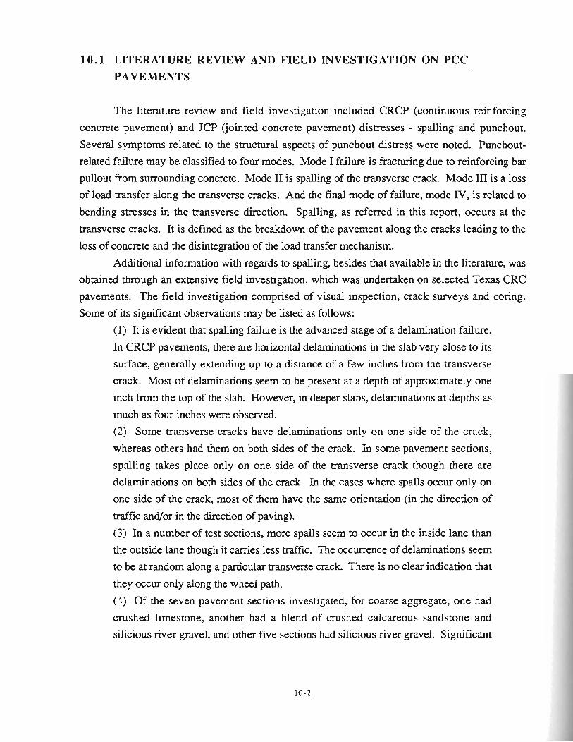
10.1 LITERATURE REVIEW AND FIELD TNVESTIGATION ON PCC PAVEMENTS

The literature review and field investigation included CRCP (continuous reinforcing

concrete pavement) and JCP (jointed concrete pavement) distresses - spalling and punchout.

Several symptoms related to the structural aspects of punchout distress were noted. Punchout-

related failure may be classified to four modes. Mode I failure is fracturing due to reinforcing bar

pullout from surrounding concrete. Mode 11 is spalling of the transverse crack. Mode 11. is a loss

of load transfer along the transverse cracks. And the final mode of failure, mode IV, is related to

bending stresses in the transverse direction. Spalling, as referred in this report, occurs at the

transverse cracks. It is defined as the breakdown of the pavement along the cracks leading to the

loss of concrete and the disintegration of the load transfer mechanism.

Additional information with regards to spalling, besides that available in the literature, was

obtained through an extensive field investigation, which was undertaken on selected Texas CRC

pavements. The field investigation comprised of visual inspection, crack surveys and coring.

Some of its significant observations may be listed as follows:

(1) It is evident that spalling failure is the advanced stage of a delamination failure.

In CRCP pavements, there are horizontal delaminations in the slab very close to its

surface, generally extending up to a distance of a few inches from the transverse

crack. Most of delaminations seem to be present at a depth of approximately one

inch from the top of the slab. However, in deeper slabs, delaminations at depths as

much as four inches were observed.

(2) Some transverse cracks have delaminations only on one side of the crack, whereas others had them on both sides of the crack. In some pavement sections,

spalling takes place only on one side of the transverse crack though there are

delaminations on both sides of the crack. In the cases where spalls occur only on

one side of the crack, most of them have the same orientation (in the direction of

traffic and/or in the direction of paving).

(3) In a number of test sections, more spalls seem to occur in the inside lane than

the outside lane though it carries less traffic. The occurrence of delaminations seem

to be at random along a particular transverse crack. There is no clear indication that

they occur only along the wheel path.

(4) Of the seven pavement sections investigated, for coarse aggregate, one had crushed limestone, another had a blend of crushed calcareous sandstone and

silicious river gravel, and other five sections had silicious river gravel. Significant

spalling was only observed in the sections made with only silicious river gravel as

the coarse aggregate.

(5) Shrinkage and swelling of expansive clays in the subgrade may be a factor which contributes to spalling.

10.2 CRACK CONTROL METHODS PROPOSED FOR PCC PAVEMENTS

Since punchout, spalling and many other distresses of PCC pavements are initiated from transverse crack locations, crack control methods are proposed in this study to examine the

feasibility of improving pavement performance on the basis of improved crack patterns. Crack

control can apply to the crack pattern in CRCP pavement as well as JCP pavement to achieve a

minimal deviation in crack spacing and practically no crack randomness as well as to minimize Y-

shaped cracks. One of the crack control methods proposed is to sawcut the pavement at an early

concrete age., Conventionally, joints of JCP pavement are cut to TI4 to TI3 deep (where T is the

thickness of the pavement slab). The early-aged sawcutting proposed in this study is different. It

cuts PCC pavement only a few hours after concrete placement but produces no significant ravelling

along the sawcut path. If sawcutting is conducted early enough, a much less sawcut depth is

required because of lower strength and higher notch sensitivity of concrete. When the sawcut is

shallower, more energy will be consumed in formation of a longer vertical crack to relaxes the

restraint on the pavement. Consequently, the tendency of delamination - a pattern of cracks

developing in the direction parallel to the pavement top surface will be reduced. Since a portable

and light sawcutter is available in the market, the feasibility of this technique is apparent. In order

to understand completely the results from the field experiments established as test sections, it is

helpful to use the fracture properties of concrete in terms of different coarse aggregates and

response of the notched pavement under stresses due to temperature variation and moisture drying.

Therefore, a series of fracture tests was conducted in the laboratory, and a theoretical analysis on

the notched pavement was performed based on fracture mechanics of concrete.

Besides sawcutting on the top surface of the pavement slab, placement of crack inducers at

the bottom of orland in the middle of the pavement slab, and skewing transverse reinforcing rebars

are two other methods proposed for crack control. Since many factors are attributed to stress

formation in the pavement such as concrete hydration, moisture movement in pavement, weather

conditions (temperature and relative humidity, etc.), and restraints on the pavement, interactions of

the crack control methods with mix designs, curing methods, construction processes and weather

conditions should be monitored in the test sections being planned.

10.3 CHARACTERIZATION OF AGGREGATE TEXTURE AND SHAPE WITH FRACTALS

Description of aggregate texture and shape is a common topic for both the aggregates used

in PCC and AC mixes. Fractals provide new mathematical tools and can be implemented to image

analysis techniques so as to describe geometrical patterns of natural structures. In a previous

project at ?TI -Project 1121, "Investigation of Rutting in Asphalt Pavements", fractal dimension of

the aggregate surface was measured to give very sensitive assessments of aggregate texture.

Under this project, a technique, which was also based on fractals, was developed to describe the

aggregate shape. The shape, texture, elongation and greylevel of nine coarse aggregates including

silicious river gravel, crushed limestone and crushed sandstone, were evaluated. The major

conclusions are as follows:

(1) A function called Slope Density Function (SDF) of an aggregate projection is

defined. This function is the frequency distribution of each slope (angle) for all the

pixels extracted from the contour of the aggregate projection. The fractal dimension

of the SDF curve is used as an index to assess the aggregate shape.

(2) The fractal dimension of the aggregate surface is used as an index for the aggregate surface texture. It is measured by the brightness contrast on the

aggregate surface under appropriate light.

(3) Elongation of the aggregate is defined as the ratio of the major axis of the

aggregate over its average minor axis, which is calculated from the area of the

aggregate projection divided by its major axis. The average greylevel gives an

indication of the color of the aggregate.

(4) The shape measure or angularity measure can divide the silicious river gravel

and the crushed limestone. The latter is more angular. The texture measure can

further differentiate the river gravel and the crushed stones. The fractals-based

shape and texture measures along with traditional image processing techniques

result in an objective and comprehensive aggregate classification system.

However, for routine laboratory testing, the particle index test (ASTM D-3398) and

the fine aggregate voids test recently developed by the National Aggregates

Association may be more practical. Test results from these two test methods and

fractals-based methods should be compared in the further research.

10.4 AGGREGATE EFFECTS ON FRACTURE PROPERTIES OF PORTLAND CEMENT CONCRETE

Fracture tests based on a nonlinear fracture model for concrete - Size Effect Law - were

conducted to obtain two fracture parameters of concrete. The two parameters are: the fracture toughness (critical stress intensity factor) for the infinite specimen, K,, and the effective crack

increase at failure (length of the fracture process zone) for the infinite specimen, cf. Concrete

specimens for the fracture tests were prepared with the same mix designs as had been used in

pavement construction in Texas. In these mix designs, nine different coarse aggregates, including

silicious river gravel, crushed limestone, crushed sandstone and dolomite along with the same

cement and fine aggregate were used in each mix. For concrete of each mix design, specimens of

four or five different sizes were prepared and tested at one-day age. Then two fracture parameters were calculated based on the Size Effect Law. The KE and cf values for different mix designs well indicated the effects of those different coarse aggregates on fracture behavior. Higher values of KE and cf indicate higher levels of toughness of concrete. In addition, physical properties of all the

nine aggregates, including SSD specific gravity, bulk specific gravity, absorption capacity and

percent solid, were determined, and gradation analysis was performed for each of the nine

aggregates. Some important results may be concluded as follows: (1) The method for determining fracture parameters KIf and cf based on Size Effect

Law is applicable to both in laboratory and the construction work site.

(2) At oneday age, concrete using limestone as the coarse aggregate is tougher

than the concrete using the river gravel as the coarse aggregate, which means that as

for as crack control goes it is easier to initiate a crack in an SRG concrete than an LS concrete. Therefore, sawcut depths requirements as they currently stand appear

to be in reverse of this finding. It was observed that limestone coarse aggregates were ruptured in one-day aged concrete during the test while only the interfaces

between river gravel and mortar fractured in the river gravel concrete at the same

age.

(3) Concrete using river gravel as the coarse aggregate became tougher when part

of the river gravel is substituted by crushed sandstone. It may explain why many

spalls occur in the pavement made with only river gravel as the coarse aggregate

while no si*cant spalling takes place in the pavement made with a blend of river

gravel and crushed sandstone as the coarse aggregate. (4) The K I ~ and cf values at early ages of concrete can be used as criteria to

evaluate concrete quality, especially when cracks at the concrete early ages are to be

controlled. However, more tests needed to identify factors such as aggregate size,

waterjcement ratio, etc., that affect these two parameters.

(5) Fracture tests of concrete specimens at ages from half a day to twenty-eight days showed that K I ~ and cf increase with the concrete age. Very early-ages

concrete is more brittle than it is at 28 days of age. Concrete may behave as a brittle

material rather than a quasibrittle material while it is at an early age so that linear

fracture mechanics may apply to the concrete pavement at the very early ages.

10.5 FRACTURE ANALYSIS ON PCC PAVEMENT SAWCUT DEPTH AND SPACING REQUIREMENTS

An fracture mechanics analysis for determining sawcut depth and spacing for PCC

pavement was fulfilled with using the experimental data obtained in the fracture tests as the fracture criterion. The results of the analysis showed that, if the pavement is cut as early as at ages of half a

day to one day, the sawcut depth of 1 inch is deep enough for a 10-inches thick pavement slab to

induce a controlled crack through to the bottom of the slab under certain environmental conditions.

Some major conclusions are achieved as follows:

(1) The Size Effect Law (SFL) - a nonlinear fracture model for concrete describes fracture behavior of concrete more precisely than the linear elastic fracture

mechanics (LEFM). The strength (the maximum normal stress) of a notched

concrete pavement slab predicted by SFL is lower than that predicted by LEFM with K I ~ as the failure criterion. Contrarily, the required sawcut depth predicted by

LEFM with K I ~ as the failure criterion must be deeper than that predicted by SEL.

In other words, the sawcut depth determined in this project by applying LEFM plus K I ~ must guarantee unstable cracking to occur from the sawcut tip through to the

bottom of the concrete slab. However, the difference between the sawcut depths

predicted by the two different approaches cannot be significant, if sawcutting is

executed early enough, because concrete is very brittle at the very early ages, as

observed in the fracture tests under this project, and, therefore, LEFM is quite

accurate to the pavement at very early concrete ages.

(2) Application of linear elastic fracture mechanics to the early-age pavement provides a convenience in stress analysis since the principle of superposition is

valid.

(3) Heat generated by concrete hydration tends to increase the temperature in the

concrete pavement. As the temperature drops, tensile thermal stresses are formed in

the pavement near its top surface. Also dqing shrinkage of concrete induces tensile

stresses in the pavement. When the stress intensity factor at the sawcut tip, KI,

reaches a critical value KIf, unstable cracking can initiate. Since the younger the

concrete is, the lower the KIf value, as is concluded from the fracture tests, a

shallower cut depth is required when cutting is performed earlier,

(4) If it is assumed that a temperature drop causes a temperature difference of 30°F between the bottom and top surfaces of the slab and the relative humidity in the

concrete pore structure at the top surface of the slab decreases from 100% to 90%,

the sawcup depth of about 1 inch is required for a ten-inches thick pavement slab.

In the same case, a sawcut spacing of about thirteen feet is required so that no

cracks will occur between the sawcuts at the early ages.

(5) Because of the size effect of the strength of concrete structures, even a less

sawcut depth is required for a thicker pavement slab.

(6) The hydration process and the drying process in concrete are complicated and

worthwhile to further investigate. More accurate data may result from numerical

analysis based on more accurate mathematical models for hydration and drying

shrinkage.

10.6 ANALYSIS OF THERMAL STRESSES IN CONCAVE CURLED CONCRETE SLAB

In order to determine the sawcut depth and spacing as well as to monitor performance of

PCC pavements, it is essential to be able to predict thermal stresses in the pavement slab with the

measurements of temperatures in it. The Westergaard solution has been widely used to the curling

analysis, where a spring model is assumed to present the subgrade support as a Winkler

foundation. However, the Westergaard solution is not valid when a gap occurs between the

bottom of the slab and the subgrade. Theoretical analysis under this project gives a complete

solution for the concave curling of the concrete slab. Based on the solution, the following

conclusions can be obtained:

(1) A concrete pavement curls to a concave configuration when it is subjected to a

negative temperature gradient, which results when the temperature at its bottom

surface is higher than at its top surface. When the temperature difference between

the bottom and the top slab surfaces exceeds a critical value, a gap forms between

the bottom of the slab and the subgrade.

(2) This critical value for the temperature difference depends on concrete elastic

constants and density, the thermal expansion coefficient of the concrete, thickness

of the pavement, and the modulus of the foundation support.

(3) If the temperature difference is below the critical value, the Westergaard solution is valid. If the temperature difference is over the critical value, the

analytical solution given by this study may be used for both displacement and stress

distributions.

10.7 TWO-DIMENSIONAL ANALYSIS OF CRC PAVEMENT AT EARLY AGES

A procedure for numerical analysis framework is developed with the two-dimensional finite element method to determine shrinkage strains and the corresponding tensile stresses in reinforced

concrete slabs. Variations of the strains and stresses with ambient climatic conditions are

predicted. A shrinkage model suggested by Ba-ant and Wu, and Ba-ant and Panula is applied. A

diffusion theory proposed by Ba-ant and Najjar is used to describe diffusion process. Creep due

to thermal and shrinkage strains is considered. The method of superimposition of virgin creep

curves is applied in this analysis and is similar to Grzybowski's analysis. Stress transfer between

steel and concrete due to bond is modelled by using a bond slip element, suggested by Ngo, which

has two degrees of freedom per node or four degrees of freedom per element at the interface of

concrete and steel elements. Following are the conclusions arrived from the analysis of example

problems:

(1) Vetter's equations may be used for predicting the average tensile stress in the

middle of crack spacing; however, it is observed that due to the bond between steel

and concrete, maximum tensile stress in concrete is observed at the level of steel for

pavements with 2" cover and in the middle of crack spacing for 6" slab and is more

than the average tensile stress. Hence, for detailed stress analysis in the prediction

of cracking, uniform shrinkage considered in Vetter's equation may not be

applicable.

(2) The cover provided to the reinforcement may become a significant factor inpavement design, especially under field conditions, where the variation of

temperature over a day is more than what is assumed, that is 30 "F over a twenty

four hour period.

(3) More detailed research should be performed toward determination of the bond-

slip relationship, because of its effect on stress distribution in concrete.

(4) Nonlinear stress-strain equations may have to be performed for the crack initiation and propagation problems instead of elastic approach considered in the

present analysis.