Embed Size (px)
Citation preview
Department of Computer Science
Alba Batlle Linares and Jonas Karlsson
Evaluation of TCP Performance in hybrid Mobile Ad Hoc Networks
Computer Science D-level thesis (20p)
Date: 06-06-08
Supervisor: Andreas Kassler
Examiner: Donald F. Ross
Serial Number: D2006:05
Karlstads universitet 651 88 Karlstad Tfn 054-700 10 00 Fax 054-700 14 60
[email protected] www.kau.se
Computer Science
Master’s Project
D2006:05
Alba Batlle Linares and Jonas Karlsson
Evaluation of TCP Performance in hybrid
Mobile Ad Hoc Networks

© 2006, Alba Batlle Linares, Jonas Karlsson and Karlstad University
Evaluation of TCP Performance in hybrid
Mobile Ad Hoc Networks
Alba Batlle Linares and Jonas Karlsson

ii
This report is submitted in partial fulfilment of the requirements for the
Bachelor’s degree in Computer Science. All material in this report which is
not my own work has been identified and no material is included for which
a degree has previously been conferred.
Alba Batlle Linares and Jonas Karlsson
Approved, 2006-06-08
Advisor: Andreas Kassler
Examiner: Donald F. Ross
iii
Abstract
Nowadays a lot of research efforts focus on Mobile Ad-hoc NETworks (MANETs). A MANET
is a collection of mobile autonomous nodes, which can move arbitrary, leading to a
constantly changing network topology. However, today most of the information is still stored
on wired servers. A wired network has a hierarchical topology, while in a MANET the
topology is usually flat to allow for nodes to easily change there position in the network. Due
to the different topological natures of these systems, interconnectivity is not trivial.
To further complicate the situation the Transmission Control Protocol (TCP) is designed for
wired networks, in a MANET with different link and route characteristics, as multihop and
frequent packet losses, the performance of current TCP proposals drop considerably.
The purpose of this report is to give an overview of the current MANET – Internet
connectivity situation and to evaluate TCP performance in a hybrid MANET where mobile
nodes connect to a wired network through a gateway.
The report is divided into two parts. The first theoretical part will evaluate the different
routing and mobility problems that occur in a realistic scenario with multiple gateways. Main
problems that will be discussed are: path selection, gateway discovery, handover between
gateways and address configuration in current solutions.
In the last part, a simulation-based evaluation will be made on a simplified scenario where
one gateway is linking the two different networks. The simulation will be conducted with ns-
2.28, which is extended with support for Uppsala University version of Ad-hoc On-demand
Distance Vector (AODVUU) as routing and gateway discovery protocol and TCP AP
(Adaptive Pacing) as transport protocol. In the performance evaluation, AODVUU and
Destination-Sequenced Distance-Vector Routing (DSDV) combined with TCP Newreno, TCP
Vegas and TCP AP will be used. The simulation based evaluation concluded that the best
performance was achieved with TCP Vegas in conjunction with AODVUU.
iv
Contents
1 Introduction ....................................................................................................................... 1
2 Background........................................................................................................................ 3
2.1 Introduction................................................................................................................ 3
2.2 Addressing ................................................................................................................. 5 2.2.1 Hierarchical/Flat Addressing2.2.2 Address Autoconfiguration
2.3 Routing and TCP in a MANET ................................................................................. 8 2.3.1 Routing2.3.2 TCP
2.4 Interconnection and Mobility .................................................................................. 10 2.4.1 Gateway Discovery2.4.2 Handover Strategy2.4.3 Mobility Management and Mobile IP
2.5 Summary.................................................................................................................. 14
3 State of The Art ............................................................................................................... 14
3.1 Introduction.............................................................................................................. 14
3.2 Addressing ............................................................................................................... 15 3.2.1 Mobile IP support IPv63.2.2 Address Autoconfiguration
3.3 Interconnection and Mobility .................................................................................. 19 3.3.1 Handover3.3.2 Interconnectivity3.3.2.1 Default Route
3.3.2.2 Half-tunnelling
3.3.3 Gateway Discovery3.3.3.1 Gateway and Address Autoconfiguration for IPv6 Ad Hoc Networks
3.3.3.2 Global Connectivity for IPv6 Mobile Ad Hoc Networks
3.3.3.3 Other Approaches
3.4 TCP.......................................................................................................................... 28 3.4.1 TCP FeW3.4.2 TCP Vegas
v
3.4.3 TCP AP3.4.4 TCP with ELFN3.4.5 A Comment on MAC Layer Unfairness
3.5 Summary.................................................................................................................. 33
4 Simulation setup .............................................................................................................. 34
4.1 Introduction.............................................................................................................. 35 4.1.1 Objectives
4.2 Simulation Environment.......................................................................................... 36 4.2.1 Mobility Scenarios4.2.1.1 Chain5
4.2.1.2 Chain5+1
4.2.1.3 Grid7x7
4.2.1.4 Random48
4.2.2 Traffic Scenarios
4.3 TCP Variants ........................................................................................................... 42 4.3.1 TCP Newreno4.3.2 TCP Vegas4.3.3 TCP AP
4.4 Routing and Gateway Discovery ............................................................................. 44 4.4.1 AODVUU
4.5 Description of the Simulations ................................................................................ 45
4.6 Simulation scripts .................................................................................................... 48 4.6.1 Traces4.6.2 Formulas4.6.3 Running the Simulation and Post Processing
4.7 Summary.................................................................................................................. 50
5 Evaluation of Simulations............................................................................................... 50
5.1 Introduction.............................................................................................................. 50
5.2 Performance parameters .......................................................................................... 51
5.3 Chain5: Simulation 1 ............................................................................................... 52 5.3.1 Congestion Window5.3.2 Throughput5.3.3 Goodput5.3.4 Average and Aggregate
5.4 Chain5+1: Simulation 5........................................................................................... 57 5.4.1 Congestion Window5.4.2 Throughput5.4.3 Goodput5.4.4 Average and Aggregate
5.5 Grid7x7: Simulation 9 ............................................................................................. 64 5.5.1 Congestion Window5.5.2 Throughput5.5.3 Goodput5.5.4 Average and Aggregate
5.6 Random48: Simulation 13 ....................................................................................... 69
vi
5.6.1 Congestion Window5.6.2 Throughput5.6.3 Goodput5.6.4 Average and Aggregate
5.7 Jain’s Fairness Index for all Mobility Scenarios ..................................................... 74
5.8 Summary.................................................................................................................. 75
6 Conclusions and Future Work....................................................................................... 78
6.1 Conclusions.............................................................................................................. 78
6.2 Future work.............................................................................................................. 80
7 References ........................................................................................................................ 80
8 Appendix .......................................................................................................................... 84
A Common Abbreviations.................................................................................................. 84
B Template Simulation details........................................................................................... 85
C Simulation scripts............................................................................................................ 94
C.1 Variables .................................................................................................................. 94 C.1.1 Traffic filesC.1.2 TCP variants
C.2 Calculations and Measurements .............................................................................. 96
D Code.................................................................................................................................. 98
D.1 Main script ............................................................................................................... 98
D.2 Simulation runner .................................................................................................. 116
D.3 Postprocess ............................................................................................................ 118
E Traffic Files.................................................................................................................... 129
E.1 1-tcp-between-node-5-node-0................................................................................ 129
E.2 1-tcp-from-node-0.................................................................................................. 129
E.3 1-tcp-from-node-0-1-tcp-between-node-4-node-0................................................. 129
E.4 1-tcp-from-node-5.................................................................................................. 130
E.5 2-tcp-from-node-0-node-4 ..................................................................................... 131
E.6 2-tcp-from-node-0-node-4-simultaneous............................................................... 131
E.7 2-tcp-from-node-0-node-5 ..................................................................................... 132
E.8 2-tcp-from-node-0-node-5-simultaneous............................................................... 133
F Scenario files .................................................................................................................. 135
F.1 chain5.dst ............................................................................................................... 135
F.2 chain51.dst ............................................................................................................. 135
F.3 grid7x7.dst ............................................................................................................. 136
vii
F.4 rand48.dst............................................................................................................... 139
G Simulation Summary .................................................................................................... 140
G.1 Description of Simulation table ............................................................................. 140
G.2 Description of Simulation Graphs ......................................................................... 140
G.3 Summary Table of Simulations ............................................................................. 141
G.4 Simulation Graphs 100Mb, 2 ms........................................................................... 143 G.4.1 Congestion WindowG.4.2 ThroughputG.4.3 Goodput
G.5 Simulation Graphs 756Kb, 25 ms.......................................................................... 238 G.5.1 Congestion WindowG.5.2 ThroughputG.5.3 Goodput
viii
List of Figures
Figure 1 Flow of packets via a MANET – Wired Gateway..................................................4
Figure 2 Handover [43] ....................................................................................................... 11
Figure 3 Network implementing Mobile IP [42]................................................................. 16
Figure 4 Address tree routed at the gateway (adopted with permission from [38])............ 18
Figure 5 Handover [10] ....................................................................................................... 19
Figure 6 Prefix Continuity [44] ........................................................................................... 24
Figure 7 Optimal window size for low BWD [21].............................................................. 28
Figure 8 TCP window size over time [21] .......................................................................... 29
Figure 9 Window sizes for different α values in a low BWD multi-hop network [21]....... 30
Figure 10 Simulation using the mobility scenario Chain 5 ................................................. 37
Figure 11 Simulation using the mobility scenario Chain 5+1............................................. 38
Figure 12 Simulation using the mobility scenario Grid 7x7 ............................................... 39
Figure 13 Simulation using the mobility scenario Random 48 ........................................... 40
Figure 14 Congestion window in simulation 1.................................................................... 52
Figure 15 Throughput simulation 1..................................................................................... 53
Figure 16 Goodput in simulation 1...................................................................................... 54
Figure 17 Average congestion window Chain5 .................................................................. 55
Figure 18 Aggregate throughput Chain5............................................................................. 55
Figure 19 Aggregate goodput Chain5 ................................................................................. 56
Figure 20 Aggregate goodput Chain 5 DSDV .................................................................... 56
Figure 21 Speed of Mobile Node 5 over time ..................................................................... 57
Figure 22 Magnification of Simulation 5 throughput.......................................................... 58
Figure 23 Congestion window in simulation 5................................................................... 59
Figure 24 Throughput simulation 5..................................................................................... 60
Figure 25 Goodput in simulation 5...................................................................................... 61
Figure 26 Average congestion window Chain5+1 .............................................................. 62
ix
Figure 27 Aggregate throughput Chain5+1......................................................................... 62
Figure 28 Aggregate goodput Chain5+1 ............................................................................. 63
Figure 29 Aggregate goodput Chain5+1 DSDV ................................................................. 63
Figure 30 Congestion window in simulation 9.................................................................... 64
Figure 31 Throughput in simulation 9................................................................................. 65
Figure 32 Goodput in simulation 9...................................................................................... 66
Figure 33 Average congestion window Grid 7x7................................................................ 67
Figure 34 Aggregate throughput Grid 7x7 ......................................................................... 67
Figure 35 Aggregate goodput Grid7x7................................................................................ 68
Figure 36 Aggregate goodput Grid7x7 DSDV.................................................................... 68
Figure 37 Congestion window in simulation 13.................................................................. 69
Figure 38 Throughput in simulation 13............................................................................... 70
Figure 39 Goodput in simulation 13.................................................................................... 71
Figure 40 Average congestion window Random 48 ........................................................... 72
Figure 41 Aggregate throughput Random 48...................................................................... 72
Figure 42 Aggregate goodput Random 48 .......................................................................... 73
Figure 43 Aggregate goodput rand48 DSDV...................................................................... 73
Figure 44 Jain's Fairness index............................................................................................ 74
Figure 45 Jain's Fairness index DSDV................................................................................ 75
Figure 46 Comparison between two different wired-bandwidths in simulation 1 .............. 76
Figure 47 Comparison between two different wired-bandwidth in simulation 1 DSDV.... 76
x
List of tables
Table 1 Common address field of an IPv4 header................................................................ 6
Table 2 Template simulations.............................................................................................. 45
Table 3 Speed of Mobile Node 5 over time.......................................................................... 57
Table 4 Number of hops for Mobile Node 5 with TCP Vegas............................................. 58
Table 5 Abbreviations.......................................................................................................... 84
Table 6 Abbreviations for Table 7..................................................................................... 140
Table 7 Table of Simulations............................................................................................. 142
1
1 Introduction
A MANET (Mobile Ad-hoc NETwork) is a network that consists of autonomous mobile
wireless nodes that can communicate without the need of a central point of coordination. This
differs from traditional wireless networks which normally need an Access Point or Base
Station and is therefore dependent on an existing wired network. A difference from an ad hoc
network is that a MANET, for abbreviations see Appendix A, must support changing network
topologies, as all nodes are allowed to move and attach at arbitrary points in the network.
The need for MANETs originally came from the need in a military and emergency
situation to quickly build a functional network without the need of any existing infrastructure.
Today, the use for MANETs has been extended to be able to provide cheap and global access
to the Internet, among other things.
When a MANET is interconnected with the Internet, or another wired network, this is
called a hybrid MANET as there is one or more special node(s) called gateway(s) that can
understand, and translate between wired network and MANET protocols. In following
chapters it is assumed that most of the traffic crosses the border between the MANET and the
Internet.
In a hybrid MANET, nodes must be able to find routes towards the Internet passing
through gateway nodes. Before to communicate however, the nodes must discover where the
gateway is located in the MANET. Gateway discovery, constant routing changes and lack of a
central point of coordination, these are all the new challenges that do not exist in a wired
network.
In a typical MANET environment, as an 802.11b WLAN in ad hoc mode, the node has
shared access to an unstable, lossy, half duplex link of around 2 Mb. In a typical wired
network, as an Ethernet LAN, every node has exclusive access to a stable, low loss, duplex
link of around 100Mb. The current transport protocols, as most TCP variants, are mostly
developed and fine tuned for wired networks, so they are not always directly applicable in a
MANET environment.
The common de-facto standard for reliable transport layer in the Internet is TCP, and UDP
is typically used for unreliable end-to-end delivery of multimedia data. As UDP cannot
provide performance guarantees. UDP usually starves TCP when competing for resources in
the same network. Therefore, extensions of UDP are used for multimedia transport such as the
2
real-time protocol (RTP) together with RTCP which provides feedback on QoS delivery and
enables rate control for better coexistence with TCP. Classical TCP performance degrades
significantly in isolated ad-hoc networks mainly due to TCPs inability to distinguish between
packet loss caused by congestion and by other factors intrinsic to multihop networks. In
MANETs, a significant portion of packet losses are caused by link failures either due to high
bit error rate, mobility of nodes or network partitions. Another source of problems is the
complex cross-layer interaction between the MAC, routing and transport layer. When TCP
probes for bandwidth aggressively during the slow start phase, there is a high probability for
MAC layer contention induced packet loss, which will cause the routing protocol to trigger
route error messages even if the route is still valid thus increasing the problem even more.
When TCP starts to react, the routing protocol might already use a different route, which
causes unnecessary route changes, even in static scenarios, and large oscillation of the
congestion window size. Several solutions for TCP as well as new transport layer protocols
have been proposed that try to avoid the problems of TCP. In order to decrease the
incompatibility issues, it is desirable that transport protocols for hybrid MANETs are
compatible with TCP.
Therefore, the problem statement of this thesis can be formulated as:
The reminder of this thesis is structured as follows. In Chapter 2, the background and some
of the different problems with the interconnection between a MANET and a wired network,
as transport protocols, addressing, routing, gateway discovery and handover, are discussed.
In Chapter 3 the discussion from Chapter 2 will be continued and extended with a
presentation of some promising proposals, like Mobile IP [18], half tunnelling [26],
AODVUU [40], TCP Vegas [4], TCP AP [6], TCP FeW [22] and more general proposals,
aimed to solve several problems, like “Gateway and address autoconfiguration for IPv6
The purpose of this thesis is to give an overview of the current MANET – Internet
connectivity situation and to evaluate how different TCP variants, perform in a hybrid
MANET, measured in terms of throughput, goodput and fairness.
To present the current MANET – Internet connectivity situation a sum up of current
“state of the art” proposals will be done.
A simulation-based evaluation study will be conducted, by performing different
simulations in a hybrid MANET environment using ns2 [41].
3
adhoc networks” by Jelger et al. [16] and “Global connectivity for IPv6 Mobile Ad Hoc
Networks” by Wakikawa et al [37].
In Chapter 4, the simulation setup is presented, as mobility, traffic scenarios as well as the
TCP variants and routing protocols used in the different simulations.
There will also be a short description of the scripts used to produce the simulations.
Chapter 5 evaluates and shows the result of a subset of these simulations, with graphs
showing congestion window, throughput and goodput.
The last Chapter 6 concludes and summarizes the theoretical overview and the simulation
results, as well as presenting future work.
2 Background
In this Chapter the underlying problems and difficulties concerning MANET - Internet
connectivity will be introduced.
2.1 Introduction
Nodes in a hybrid MANET need to communicate with fixed hosts in the Internet. Today one
of the most used transport protocols in Internet is TCP. Few studies as [35] have been made
on the performance issues that occur, when connecting a MANET to the Internet and those
only have been mainly focused on UDP. UDP does not need to re-establish a new connection
at each address change or resend lost packets, as UDP does not guarantee delivery and
therefore does not use ACK or other mechanisms to recover from lost packets. Because of this
connectionless behaviour, UDP does not suffer from the address changes that happen in a
MANET as much as TCP does.
TCP uses a connection oriented approach where packets flow from a sender to a
destination node, where each flow is identified by certain parameters, with the IP-address
being one of them. A change of the IP-address will therefore cause a drop of that connection.
Another issue with TCP is that it uses a congestion control that is not adapted to a MANET
environment and as a result, TCP sometimes will not use the entire available network
capacity. Therefore, this study will concentrate on TCP performance in MANET – Internet
connectivity and gateway discovery.
In general, MANETs do not incorporate the term of subnets as wired IP networks do.
Instead, a MANET has a completely flat topology where the only requirement for a node is
4
that its address is unique within that MANET. This makes sense as nodes are mobile and can
attach at arbitrary points to the MANET. Therefore, routing protocols must cope with this
new addressing structure.
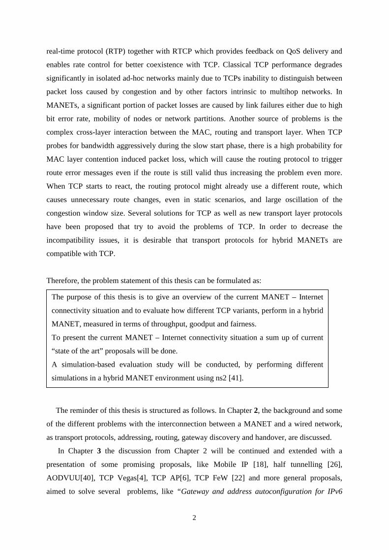
The intersection between a MANET and a wired network is a node called gateway or
access router, which has at least the functionality of translating addressing structures, routing
protocols, and physical network interfaces between the two networks, see Figure 1.
Figure 1 Flow of packets via a MANET – Wired Gateway
The number of gateways depends mainly on the area that the network is supposed to cover,
radio propagation and node density. However, having multiple gateways introduce new issues
e.g. handover and gateway discovery, as will be presented in more detail in Chapter 2.4.2 and
2.4.1.
A simple solution to interconnect a MANET with a wired network would be to let a
gateway act as a proxy and do network address translation, and answer all route requests that
it knows belong to an Internet address. However, this means that, when using a reactive
routing protocol see Chapter 2.3.1, the MANET nodes, because of the flat addressing
structure in a MANET see Chapter 2.2.1, cannot distinguish between wired and MANET
nodes. The gateway must keep an entry in the routing table for each of the different
connections [24]. The result of this invisibility forces the mobile node to send a route request
every time a packet should be routed to a new Internet node. Depending on the scenario, this
will cause a flood of route request in the MANET; also the routing tables will increase.
This simple solution, although theoretically feasible, will also cause inefficiency with
mobility. Even if there is another gateway fewer hops away from the mobile node, packets
will always be routed through the same gateway and a not optimal path through the low

5
bandwidth MANET will be used. In a more realistic scenario, the node would change gateway
either because it loses the link or to improve performance.
Tests have shown that the throughput of TCP roughly follows a 1/n curve where n is the
number of hops [32], when the nodes are connected in a “linear” chain. This means that
everything else the same, there is only about 1/3 of the throughput left, when there are 3
wireless hops between the sender and receiver. Therefore, short hop distance to the gateway is
crucial for an efficient Internet connectivity. This will be treated in more detail in Chapter.
2.3.2.
This suggests that some sort of gateway discovery algorithm to find the closest gateway
should be performed and the closest gateway should be chosen as efficiently as possible to
minimize MANET traffic. However, allowing the mobile node to change gateway will break
ongoing TCP connections, as the Internet node only knows the IP address of the gateway,
which acted as proxy for the mobile node. In case Mobile IP [18] is used to maintain the TCP
connection, an increased overhead will be the result, as a re-registration with the new gateway
is necessary. The advantage with Mobile IP is that each node in the MANET maintains the
same IP address independently of the gateway attached.
If not Mobile IP is used it leads to another problem, what IP address will the mobile node
have in the Internet? In the simple scenario described here, the gateway does NAT and acts as
a proxy but as we have seen, this has its drawbacks. A closely related problem is as
mentioned before how the mobile node gets its unique address within the MANET.
A lot of research is focused on MANET connectivity; although some solutions exist to solve
these problems today [16] [37], they all have there deviances [35] and a lot still remain to be
solved.
The rest of this chapter will describe in more detail the problems mentioned and discuss
the impacts they have on network connectivity and performance.
2.2 Addressing
An ideal IP address would be unique, globally routable and location independent as mobile
nodes move in and between MANETs and connect to different gateways.
The fact that it is common that mobile nodes in a MANET use IP addresses does not mean
that it is straightforward to interconnect a MANET with a wired infrastructure [35].

6
IPv6 has some extended capabilities, e.g. address autoconfiguration and extended address
space over IPv4, which some proposals use to more easily circumvent the differences between
hierarchical and flat structures [35].
2.2.1 Hierarchical/Flat Addressing
One of the main problems is that in a wired IP network, the addressing scheme is
completely hierarchical and nodes belong to subnets which are interconnected via gateways.
110 NET–ID SUBNET-ID NODE-ID
Table 1 Common address field of an IPv4 header1
The IP address is not only a unique identifier2 but it also devotes the place the node have in
the network hierarchy, so every node routes the packets through a known default gateway, if
the IP address is not within its own subnet. If the packets come from one of the gateway’s
subnets it relays them out on that subnet, otherwise it sends them to its own default gateway
and so on. This is also known as longest prefix matching and is similar to how a post address
works when you post a letter3.
The decision to route the packet to the gateway or not is usually solved by having a specific
subnet mask on each node that is evaluated against the nodes own IP address and the IP
address of each sent packet. If there is a mismatch, that packet belongs to the “outside” and is
routed through the nodes default gateway. This scheme, although very efficient where nodes
and gateways are static, has its limitations as it does not allow nodes, and in particular not
gateways, to attach at different points in the network without reconfiguration of the IP
addresses.
Within a MANET where there are high mobility and many nodes, link and route changes
would occur frequently, which makes the cost of maintaining a hierarchical tree structure too
high in most cases [37].
So instead, in a MANET a flat address topology is used where the IP address only is a
unique identifier for that node and does not carry any network topology information. This is
beneficial as it minimizes the impact of route changes, at a cost of slightly more complicated
routing. However, this also implies that there is a conceptual difference between hierarchical-
1 Net-id, which is the identifier that the routers in the internet base their routing information, combined with
subnet-id determines the nodes place in the hierarchy. 2 In that particular network 3 In Sweden 20060215
7
IP and flat-IP, which could not easily be overcome as hierarchical-IP nodes will not recognize
MANET nodes with an IP address not belonging to the same subnet as its gateway4 [38].
The most appealing approach to solve the problem with nodes changing subnets would be to
route the packets through the MANET and use the same gateway during the entire
connection. As mentioned before, the most beneficial is to use the closest gateway to the
Internet. However, there is always a trade off between the number of hops and the overhead in
changing gateway as will be explained further in Chapter 2.4.2.
2.2.2 Address Autoconfiguration
Address autoconfiguration is the procedure that a node uses to get, and configures, its IP-
address. In a traditional wired IPv4 network, this was achieved using a central DHCP server,
which assigned IP-addresses to the nodes. This is also called stateful autoconfiguration. This
method works well for fixed networks as partitions rarely happen and as nodes are mostly
stationary so IP-address requests seldom occur. Therefore, the overhead of the DHCP requests
will be small and congestion will not be a problem.
For a MANET however, the situation is completely different, network partitions and
merges occur frequently as nodes move within the MANET. Address requests are therefore
assumed frequent so this approach is not suitable for MANETs due to the risk for congestion
and loss of packets. In a MANET, there is also no easy way of obtaining which DHCP server
to use because of mobility and flat addressing structure.
The second approach is stateless auto-configuration, which was incorporated in the IPv6
standard, where a node auto-configures an IP address without help from a central entity (as a
DHCP server). However, the IPv6 auto-configuration mechanism is developed for one-hop
networks and therefore only allows nodes to generate a link-local address, and do not take
into consideration multihop networks. Modifications to this mechanism [17] [30] [37] exists,
which will be described in more detail in Chapter 3.2.2
As no central entity dictates IP addresses, depending on the solution of auto-configuration
parameters, the problem of duplicate addresses can occur. In those cases, some duplicate
address detection (DAD) must be employed.
As a general, but not mandatory, rule it is best to let the mobile node belong to the same
subnet as its default gateway as this simplifies filter and routing management. This is the
same as giving a mobile node a globally routable IP-address. Unfortunately, this conflicts
4 Unless the gateway does some sort of NAT, as will be shown in later chapters this only postpones the problem.
8
with changing the gateway during a connection, because this involves changing IP-address of
the node [35].
2.3 Routing and TCP in a MANET
In this chapter, we will present some of the problems with TCP and routing in a MANET.
2.3.1 Routing
MANETs have their own routing protocols mainly due to their flat structure of the
addresses and mobility. Some of them are invented or just adapted from wired protocols [27].
All protocols must follow some principles to be beneficial for an ad-hoc network such as to be
adaptive to a dynamic topology or scalable with the number of nodes. Furthermore, the main
challenge for a routing protocol is to be able to represent the current topology at all time.
Routing protocols in MANETs are classified in three different groups: Proactive, reactive
and hybrid. This classification is done based on how the protocol works to find a proper path
for a concrete destination.
Proactive protocols follow the same philosophy as link-state and distance vector protocols
used for wired networks; each node of the network has its own table with all neighbour nodes
and the cost of each different path. The primary problem in proactive routing protocols is that
every intermediate node has to update constantly a table with all the information about other
nodes in the network. Moreover, each time control messages are sent in the network, this
excess of information, may generate congestion in the network and loss of data packets due to
buffer overflows and MAC contention. The maintenance of the paths is expensive because
constantly routes can be broken because of the nodes’ mobility, which generate constant
updates of information in each node. Therefore, link-state protocols are not suitable in high
mobile MANET, with many route table changes, because in each node topology information
is replicated. Examples of proactive routing protocols are DSDV and OLSR.
Reactive protocols or on demand, start a route discovery each time that they have a packet
to send to a destination and its route is not known. Usually, nodes that implement reactive
protocols have a cache where all the routes discovered are stored for future uses; routes not
used recently are expired even if they are still valid. The key feature of on-demand protocols
is acquiring routing information only when it is actually required, avoiding maintaining long
routing tables. Sender will have to acquire a route to the destination before the
communications start which suppose an increase of the transmission time for the first packet.
9
The goal of an on-demand protocol is to offer optimal path for each node that requires it,
without having obligation to maintain updated information. Examples of reactive routing
protocols are DSR and AODV.
Hybrid protocols use both proactive and reactive techniques. Hybrid protocols maintain
state information for neighbour links, within a limited area from the node. Route discovery is
performed to determine a path for a destination, which is far away from the source node.
All these protocols have advantages and disadvantages depending on the mobility, traffic, etc.
Example of a hybrid routing protocols is ZRP.
2.3.2 TCP
TCP was designed for wired low-loss, stable networks with a high bandwidth-delay product
(BDP, in some graphs mentioned BWD), which determines the number of packets that can be
in transit in the network. Therefore, it misinterprets many of the network characteristics when
used in a MANET environment [36]. One of the already investigated characteristic [36], is
that TCP interprets packet loss as congestion and reduce its congestion window, which is the
amount of packets that TCP will allow to be in flight in the network at the one time, to
compensate for this. In a MANET, this is far from always true as wireless links by nature are
error-prone and the correct behaviour, in the case of bit errors in the transmission, would be to
retransmit the packets immediately as fast as possible.
In a mixed environment with both UDP and TCP flows the situations become even more
troublesome [32].
Even in a single hop environment but with unreliable wireless links, TCP throughput will
suffer from successive retransmissions. If the link-layer also resends packets, this can lead to
bad protocol interaction, which causes TCP retransmission timers to expire, and make TCP
resend these packets as well. This is even more prevalent in a multihop environment as these
transmissions often collide, at intermediate nodes, with data or ACK packets. As shown in
[32] this lead to that TCP will have a throughput curve close to 1/n, where n is number of
hops.
In a MANET where nodes are mobile, link breaks are frequent, the more links (hops)
involved the higher the path break probability is [36]. Path breaks also triggers new route
requests from the network layer and if this takes more time than TCP retransmission timeout
(RTO) then TCP goes into slow start and throughput is even more decreased.
The use of a sliding window for flow control, as TCP use, requires that the link-layer
provide long- and short-term fairness for optimal performance in a low-bandwidth network.
10
The reasons for this is, that with an unfair link-layer the unfair treated nodes will assume a
congested network and back off, while the privileged nodes will send faster as they assume a
lightly loaded network. In MANETs today the ad hoc standard for the link-layer is IEEE
802.11. Unfortunately, this protocol cannot provide short-term fairness, because of the binary
exponential backup algorithm used to avoid collisions a node that has captured the channel
has greater chance of capturing it again [23]. This will create burstiness in the traffic that will
penalize TCP throughput. [36]. Interconnected with a wired network this short-term
unfairness also will lead to long-term unfairness [39].
Window size is also problematic when a MANET connects to a wired network. Tests have
shown [39] that in a pure MANET a window size of 1/3 of path length is the optimal. In a
normal MANET scenario, this evaluates to one or two as optimum. However, this is
unacceptable in a wired network where this window size will cause unacceptable low
throughput [39].
2.4 Interconnection and Mobility
To reach the Internet a node must fulfil certain criteria. A node, to be able to send packets,
must have a globally routable address and a known path or gateway to reach the destination.
To know which path to take normally a gateway discovery has to be done, as may change due
to mobility.
2.4.1 Gateway Discovery
When a mobile node should reach an Internet node; does it know if the node’s address is
within the MANET and if it does where should it send the traffic? As seen in Chapter 2.3.1,
this is not obvious and sometimes requires a MANET wide route request.
Different solutions have emerged to make the node aware of what and where to send the
traffic to reach an Internet node, mainly there are the three main approaches used in MANET
routing protocols, e.g. proactive, reactive and hybrid.
In a Proactive approach, the gateway periodically floods the MANET with HELLO
messages, which also can contain network prefixes so that mobile nodes can decide what and
where the traffic should be routed to reach the gateway. The advantage of this is that it scales
well with the number of nodes that want to reach Internet. However, it does not scale with the
total number of nodes in the MANET [34].
In a Reactive approach, the node is not aware of the route to the Internet (e.g. gateway) in
advance and therefore does a flooding route search, which the gateway answers. This has the
11
advantage that it does not create traffic unless a node really wants to reach the Internet. The
drawback is that it is not scalable in the realistic scenario when many nodes want to access the
Internet [34].
In a Hybrid approach, the gateway send proactive HELLO messages to a limited group
(e.g. the number of hops from the gateway) and let the nodes further away reactively find the
gateway. For a minimal overhead, an optimal size of the group must be found. As shown in
[34] the optimal size of the group varies depending on scenario and network condition so
some sort of estimation must be made by the gateway on these parameters.
Solutions exist [16] [37] [34] that use the above-mentioned approaches. There also exist
solutions without the need for a specific gateway discovery mechanism as they use a
hierarchical tree structured addressing and routing scheme based on MIPv6 [38]. This
however put some constrains on the allowed mobility and number of nodes in the MANET.
2.4.2 Handover Strategy
In reality, a scenario with one gateway can be found, but to extend the coverage or
performance usually several access routers or gateways are used, which connect the MANET
with the wired network.
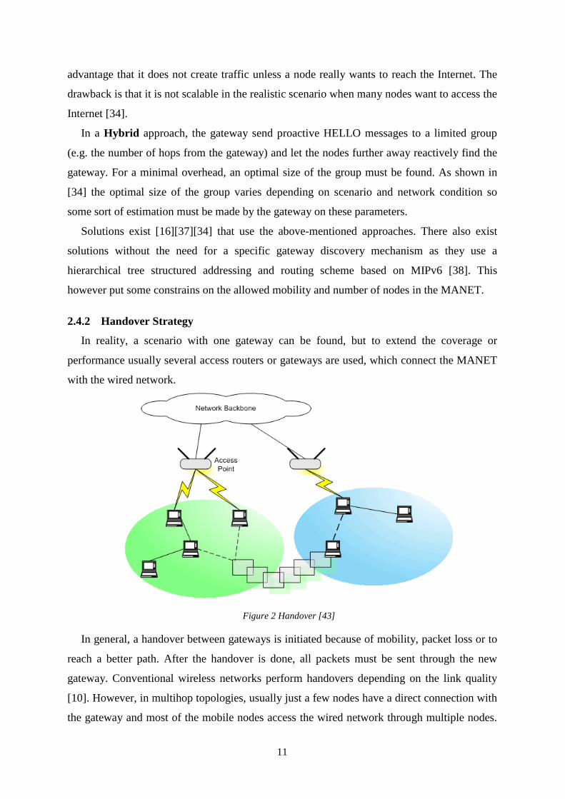
Figure 2 Handover [43]
In general, a handover between gateways is initiated because of mobility, packet loss or to
reach a better path. After the handover is done, all packets must be sent through the new
gateway. Conventional wireless networks perform handovers depending on the link quality
[10]. However, in multihop topologies, usually just a few nodes have a direct connection with
the gateway and most of the mobile nodes access the wired network through multiple nodes.
12
Sometimes handover may be useful to load balance between different gateways, avoiding
packet drops because of buffer overflow or network congestion.
Handover strategies, is a topic in research, although some protocols are already beginning
to emerge.
MRAN, Mobile Radio Access Networks [13], which offers access to the Internet for the
ad-hocnodes, presents handover maintenance and constantly tries to optimize gateway
connectivity. Two different kinds of handover can occur: Forced and optimizing handovers.
Forced handover is involuntary. In some situations, communication is not possible with
the access router due to broken route or just that a mobile node has been disconnected. Then a
new gateway discovery has to be started, just like the first time that the node appears in the
network. Forced handover is possible in all gateway discovery approaches, proactive, reactive
and hybrid.
Optimizing handover as a difference to forced handover is voluntary and is used to find a
better gateway in terms of number of hops, as well as other parameters that may be influent to
the delivery of packets. Not all gateway discovery approaches can implement this handover
because advertisements from the gateways are required, as proactive and hybrid do.
From this information, mobile nodes can decide if another gateway is better than the
current one. If Mobile-IP is used, to maintain transmissions while changing IP-address, the
mobile node will start a registration with the new access router before it breaks the link with
the old one.
It is important to determine precisely when an optimizing handover really is beneficial,
instead of waiting for a forced handover. This because each optimizing handover introduces a
delay and a break in the flow of packets transmitted. Moreover, not all the proposals allow
storing packets in a buffer (e.g. reactive and hybrid) [13] and for this reason it is possible to
have loss of packets that will cause retransmissions. In Chapter 3.3.1 these decisions of the
node will be treated in more detail, since it is important to know when it is effective to
execute an optimizing handover and how the transmission would be affected in terms of
delivery of packets, goodput and packets delay.
2.4.3 Mobility Management and Mobile IP
Nowadays, most of the research is focused on how to improve MANET performance, not its
connectivity with other networks. However, interconnectivity between MANET and wired
networks is one of the most important current problems to be solved because of the necessity
to communicate with the Internet, not only between mobile nodes. Using Mobile IP [18]
13
wired nodes could conserve their own home address in the entire network. Unfortunately,
Mobile IP, keeping this own address, does not solve all problems concerning addressing and
routing in a MANET. Several different strategies to send packets to an external node exist e.g.
default route and tunnelling.
Reactive protocols have not the possibility to determine whether a destination is a fixed
node or not. Therefore, unless reserved prefixes for MANET nodes or other similar
techniques are used, a request must be flooded through the MANET. In some cases, the
gateway will answer, offering to take care of these destinations, otherwise if the network not
replies, it is assumed that it is an external node. On the other hand, proactive routing protocols
are able to know if a node belongs to an ad-hocnetwork, by checking for each address in their
routing tables. Moreover, intermediate nodes between the source and the destination have to
keep the destination address in their routing tables for future uses and verify that is an external
node, if not a request must be flooded through the network); this phenomenon is called
“Cascading effect” [24]. Its consequence is congestion in the network and the growth of
intermediate route-tables. In the attempt of reduce the amount of request packets sent in the
network a default route is created. The default route technique is especially useful for the
packets that have the same prefix address destination and share most of the hops, avoiding
route discoveries for nodes from the same subnet. However, this method has some drawbacks
when it is used in a multiple gateway scenario, especially during a handover [26]. Some
possible solutions are presented in Chapter 3.3.2.1
Another alternative is to create a tunnel between the source and the destination, simulating
one hop communication when it actually is a multihop connection. Our study will be focused
on the “half-tunnel” proposed by Uppsala University [26]. It is called half-tunnel because
tunnelling only is performed in one way, from the mobile node to the fixed host, in the other
direction the gateway may forward information without difficulties. When a packet for a fixed
host has been detected, as explained in the above section, the packet is encapsulated with a
new header, with the gateway as a destination. Then, in the gateway, the packet is
decapsulated and the original packet will be sent to the real wired destination. With this
strategy, intermediate nodes have not to maintain any routing table. Cascading effect and
look-ups are avoided because packets will be routed to the gateway as normal packets in an
ad-hoc network, using a MANET routing protocol. A more detailed comparison could be
found in Chapter 3.3.2.2
14
2.5 Summary
As shown in this chapter there are several problems with the interconnection between
MANET and the Internet nodes.
The main problem comes from what a MANET is, namely mobile and multihop. Many of
the other problems derive from these two characteristics.
Mobility leads to the need to change the addressing structure, which in turn causes
adaptation of address auto-configuration procedures and routing protocols. Closely related to
this are gateway discovery and handover strategies, in terms of finding the optimal path to a
wired node.
Multihop effects and complicates the problems that mobility presents and in turn
introduces some new issues, as TCP performance degradation.
The proposals to solve these and the other issues mentioned will be treated in the following
chapter.
3 State of The Art
In this chapter current state of the art proposals and implementations, to problems and issues
described in Chapter 2, will be presented.
3.1 Introduction
In Chapter 2, we introduce some of the problems that can occur in a hybrid MANET
environment where there exist both wired and wireless mobile nodes. In this chapter, it will
be presented some promising proposals to solve these problems.
A brief technical overview is presented together with a short description of the
consequences that they can impose in a hybrid MANET scenario. Because some proposals not
only cover one topic, the structure of the different parts is slightly changed from Chapter 2 to
accommodate for easier understanding. To focus on our main topic some previous sections as
hierarchical/flat addressing and routing, are omitted as they will be mentioned in a context
relevant for our study.
As nodes can move freely within and between different MANETs, it is important that there
exist some mechanisms that allow the nodes to keep the connection during these transitions.
15
It is important that nodes can be reached by a permanent address so that knowledge about a
mobile node’s current gateway is not needed. For global route-ability in the Internet, it is
important that the mobile nodes have an address from the same subnet as its current gateway.
As will be shown further in Chapter 3.2 some of these requirements are fulfilled by using
Mobile IPv6 and some extension of IPv6 autoconfiguration schemes.
To reach or to be reached from the Internet, a mobile node must know or be able to
discover the route to the gateway, which interconnects the MANET and the wired Internet. In
a multiple gateway scenario it is important to know which gateway offers the most efficient
interconnection. There must also be a mechanism that is able to handle a proper switch of
gateways during an ongoing connection, to avoid unnecessary packet retransmissions.
Some solutions for gateway discovery and handover that solve these issues will be
presented in Chapter 3.3.
As explained before, the TCP protocol performance in a MANET has many issues that
degrade performance; there are other transport protocols e.g. [2] specific for MANETs that
deal with these problems. However, when a MANET is interconnected with the wired Internet
a TCP interoperable protocol is preferable, as to avoid gateways to do costly transport layer
adaptation. All of these topics are fields of research so new solutions spring forward
constantly; this chapter tries to summarize the current state of art.
3.2 Addressing
3.2.1 Mobile IP support IPv6
Mobile IP is a standard communication protocol, described in [18]. This protocol provides an
efficient mechanism to allow mobility within the Internet. Mobile IP support for IPv6 is an
adaptation of Mobile IPv4 for the new version of IP addresses, IPv6.
Nodes that implement Mobile IP can be identified by their permanent home IP address
independently of which point they use to access to the Internet.
When a mobile node changed its place in the topology and is attached to another subnet, it
is identified by a care-of address, but it still will receive packets addressed to its home
address. The visitor node obtains this care-of-address with the same mechanism as IPv6, auto-
configuration scheme; the care-of-address has the prefix of the subnet in the visiting link.
Each packet addressed to the home IP address will be rerouted to the current care-of-address,
and finally will arrive to the mobile node.
16
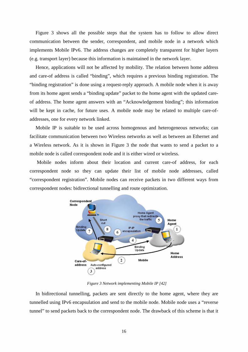
Figure 3 shows all the possible steps that the system has to follow to allow direct
communication between the sender, correspondent, and mobile node in a network which
implements Mobile IPv6. The address changes are completely transparent for higher layers
(e.g. transport layer) because this information is maintained in the network layer.
Hence, applications will not be affected by mobility. The relation between home address
and care-of address is called “binding”, which requires a previous binding registration. The
“binding registration” is done using a request-reply approach. A mobile node when it is away
from its home agent sends a “binding update” packet to the home agent with the updated care-
of address. The home agent answers with an “Acknowledgement binding”; this information
will be kept in cache, for future uses. A mobile node may be related to multiple care-of-
addresses, one for every network linked.
Mobile IP is suitable to be used across homogenous and heterogeneous networks; can
facilitate communication between two Wireless networks as well as between an Ethernet and
a Wireless network. As it is shown in Figure 3 the node that wants to send a packet to a
mobile node is called correspondent node and it is either wired or wireless.
Mobile nodes inform about their location and current care-of address, for each
correspondent node so they can update their list of mobile node addresses, called
“correspondent registration”. Mobile nodes can receive packets in two different ways from
correspondent nodes: bidirectional tunnelling and route optimization.
Figure 3 Network implementing Mobile IP [42]
In bidirectional tunnelling, packets are sent directly to the home agent, where they are
tunnelled using IPv6 encapsulation and send to the mobile node. Mobile node uses a “reverse
tunnel” to send packets back to the correspondent node. The drawback of this scheme is that it
17
introduces overhead and it will in some cases use a longer path to route the packets to the
mobile node. The advantage is that no modifications are needed at the correspondent node.
However, in route optimization, correspondent nodes previously have to support
correspondent registration. Packets are sent directly to the mobile node using the care-of
address already obtained in the registration. Using correspondent registration packets get the
care-of address of the destination node; packets are forward straight to the mobile node, called
short cut in Figure 3, avoiding intermediate nodes as the home agent. This method reduces
congestion at the home agent and improves performance because of a shorter path between
the nodes.
A variant of the IPv6 header is also added to the packet, containing the home address of
the mobile node. In that case, the mobile nodes set the source address to its care-of address.
Mobile nodes with the mechanism called “dynamic home agent address discovery”, can
discover the IP address of a home agent within their own home link, even when they are
visiting other networks.
The use of the Mobile IPv6 makes mobility transparent for layers above network layer.
Mobile IP Fast Handover protocol [20] has been developed to reduce the time when the
mobile node changes its point of attachment. A handover involves a break of packets flow,
while a mobile node registers to the new care-of address. For real-time applications or voice-
over-IP, these interruptions cannot be acceptable.
It is important that mobile nodes can trust their own home agent so they can establish
private communications. In [3] it is described a security implementation for Mobile IP that
makes it possible to do encrypting “binding updates”. Connections between mobile and
correspondent nodes have to implement more complex mechanisms to assure truthfulness. To
provide authentication nodes have to implement a “return route-ability procedure”, where
mobile nodes and home agent send cookies to the correspondent node. Then, the
correspondent node build a pair of keys that will be shared between all nodes involved in the
communication. Afterwards, the mobile node builds a binding message key that will be used
to sign the binding update message, exchanged between the nodes during the binding process.
In MANETs it is beneficial to use Mobile IP especially when multiple gateways are
involved, to keep the connection while the mobile nodes are moving between the different
gateways.
18
3.2.2 Address Autoconfiguration
As stated earlier in Chapter 2.2.2, using stateful address configuration is not suitable and
sometimes even not possible in a MANET.
To let the nodes have the same prefix as its current gateway but still change its address as
little as possible, [16] [31]have split the IPv6 address field in two 64 bit fields. A MANET
local-address field that is used for routing within the MANET and a prefix (of the current
gateway) that is added to the MANET-local address to provide global connectivity. The
MANET-local address consists in both cases of the EUI-48 (e.g. MAC) address and an added
16-bit pattern. In [31] the pattern is predefined (e.g. ff:fe) and in [16] it is a 16-bit random
number.
The decision to use a random number in [16] will, in the case of identical EUI-48
addresses (very unlikely, as the MAC address should be unique), reduce the collision
probability to 1/64536, in these cases.
Because of the low probability of address collision Jelger et al. therefore chose to do not
use a complex DAD (Duplicate Address Detection) procedure, Jelger et al. explain in [17]
why a simple DAD procedure could fail in a MANET, mainly this is because of the
continuous network divisions and merges. However, in [31] Perkins et al. use a simple DAD
procedure, where a node via a temporary address; broadcast the suggested address and if there
are no replies the suggested address is chosen by the node.
The prefix that later is added to the MANET-local address is advertised by the current
gateway to provide a global routable address. When the mobile node is attached to another
gateway, the nodes prefix will change accordingly.
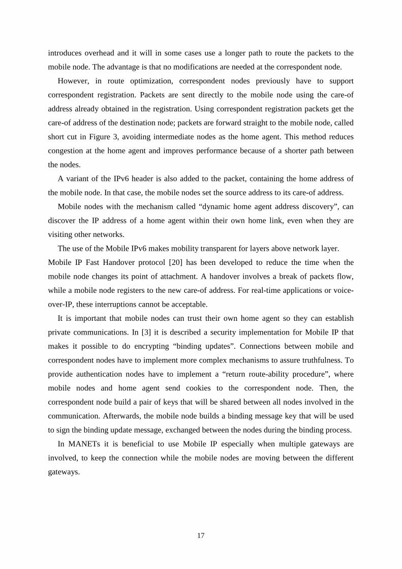
A completely different scheme (e.g. hierarchical) is used in [38] where each node acts as a
DHCP server and distributes local addresses to joining neighbourhood nodes according to its
place in the address tree, see Figure 4.
Figure 4 Address tree routed at the gateway (adopted with permission from [38])
This scheme simplifies and avoids many problems (e.g. addressing, routing and gateway
discovery) connected with MANETs. However, it also implies relatively small MANETs with
low mobility, e.g. walking speed, which is an extension of a wired infrastructure.
19
To conclude, in small MANETs, according to number of nodes, with low mobility (e.g.
with few path breaks, merges and divisions), all schemes work well. However, [38] provide
the most straightforward implementation, as it builds on well-known approaches. In a more
mobile scenario where path breaks become a burden both [16] [31] can provide a more robust
and scalable solution.
3.3 Interconnection and Mobility
3.3.1 Handover
Multihop radio access networks MRAN provide access to the Internet for mobile nodes in ad-
hocnetworks. Because of mobility, topology is constantly changing and a permanent
connection with the Internet cannot be possible through a single gateway.
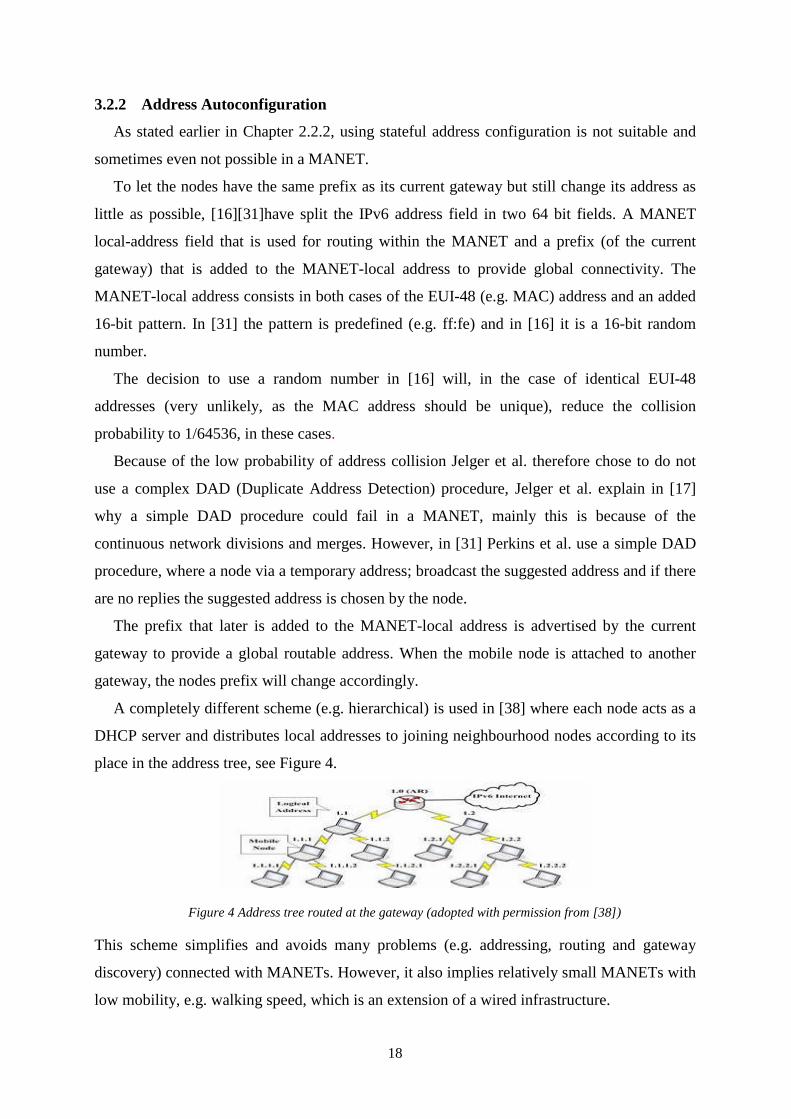
In a multiple gateway scenario, when there is a need to change gateway while packets still
are on flight, this change is called handover. As it is shown in Figure 5, MN0 performs a
handover.
Figure 5 Handover [10]
A Handover can be performed for two different reasons, because of a link breakage or to
optimize the connection.
20
Forced handovers are normally produced when the route between the mobile node and the
gateway is broken, because of nodes’ mobility, etc. This, however, requires active monitoring
for path breaks. In the case that another path to the gateway does not exist, the mobile node
starts a gateway discovery to find out the route to the closest gateway in the system. Usually
in multihop environments, mobile nodes do not have a direct connection with the gateway,
therefore it is difficult to start a handover based on link quality [10]. Links are normally
measured in terms of number of hops. Depending of the cause, handovers are classified in
forced or optimizing handovers [13]. It is hard to determine features of a route, built of
different hops. The mobile node is normally the responsible to determine when a handover
has to be done. The entire path, including all the intermediate links, should be considered
before the mobile node takes the decision of perform a handover.
With reactive routing protocols, a gateway discovery is only initiated when the mobile
node has the necessity to send some packets to the wired network. The connection with the
gateway will be used until a link breakage occurs; only then, a new route discovery is going to
be performed.
In proactive and hybrid environments, gateways send continuously advertisement
messages with information about the current number of hops from the gateway to the mobile
node. The mobile node can then compare this with the information it has about the current
gateway connection. In the case that another gateway would have a shorter path, an
optimizing handover starts. Before to break the link with the existing gateway, a registration
begins to the new gateway, when the mobile node is attached properly, then the
communication with the old gateway is ended. Using optimizing handover, the rate of forced
handovers is reduced considerably although signalling increases.
Depending on the handover decision, different kind of signalling has to be used [9]. The
signalling system used for forced handovers is divided into two phases: gateway discovery
and registration. In the first phase, the mobile node finds a new gateway while in the second
phase the node registers with the new gateway.
In the Optimizing-based handover signalling mechanism, first information from the new
gateway is received by the mobile node, when the new care-of address is already assigned to
the node a notification of the change is sent to the network to update its caches.
Optimizing handovers reduce number of hops to the gateway and improve the utilisation of
the network. However, it has to be considered that for each optimizing handover the flow
packets is broken and a delay is produced. Hence, it is crucial to define properly the optimum
situation when it is better to carry out an optimizing handover instead of waiting for a forced
21
handover. To establish the rules considered in this decision, several parameters of the network
have to be considered. Packet delivery ratio, handover delay and signalling overhead are some
of the parameters to consider before doing a handover. Packet delivery ratio refers to the
fraction between packets sent to the Internet and packets generated in the source node.
Handover delay is the time between the point, where the mobile node detects that handover
is required and the completion of the handover procedure. In forced handovers, this parameter
reflects the time it takes to discover a new gateway and register with it. However, as in
optimizing handover the gateway address is already known, the handover is determined by the
time necessary to register with the new gateway. Obviously, increasing the advertising
messages from the different gateways will give more information to reduce the delay, offering
a better path.
To guarantee an efficient network it is important to find the balance between forced and
optimizing handovers, otherwise handover delay will be increased and delivery ratio reduced.
Some studies as [9] [10] show that for identical mobility scenario proactive routing
protocols perform better than the reactive ones, in terms of packet delivery ratio and average
packet delay, as a consequence of knowing the entire network topology. In a forced handover
this means that the registration can start immediately and no gateway discovery has to be
performed first, which reduces the handover delay. The results obtained for hybrid approaches
are comprised between proactive and reactive values. Handover delay is shorter in proactive
approaches. When the link is broken another alternative can be used avoiding to start a new
gateway discovery. Nevertheless, both approaches have a similar rendition in environments
with a high number of gateways, only scalability features are lower in proactive approaches.
3.3.2 Interconnectivity
This section is based on the paper from Uppsala University [26].
Nowadays, several researchers [26] [35] are focused on finding the proper way to interconnect
Ad hoc networks and the wired Internet, because of the interminable range of possibilities that
an Internet access can offer. Because of the two different kinds of addressing, hierarchical and
flat, the principal issue is to find the location where to send the packets.
Several solutions can be performed to find the location of the correspondent node
depending on the routing protocol used in the MANET. Proactive protocols can determine if a
node is or is not within the MANET, by checking its routing table.
On the other hand, reactive protocols have to flood a request message through the
network; the absence of answers from the network usually means that the node is from the
22
wired network, although this is not 100% reliable as packet losses can occur. Broch et al. [5]
propose a more advantageous solution instead of using timeout. Here, the gateway insures
that the requested node is not in the MANET. How this insurance is done, depends on the
specific addressing scheme scenario, e.g. if all MANET nodes have a special prefix the
gateway, by looking at the address, can determine if it is a MANET or wired destination, and
replies offering itself to be a proxy for this node. During the gateway discovery it is a good
moment to notify all the intermediate nodes about the location of the wired node [26].
Intermediate nodes will then keep this information in cache for future use. However, some
devices might have limited memory capacity, so big route tables and caches seem to big high
overhead. The straightforward procedure, after the location of the node is resolved, is to find a
route to the destination and forward the packets. Intermediate nodes will keep this information
in their routing table as a one-hop destination, connected directly to the gateway. The
drawback of this solution is that intermediate routing tables will grow, and each route to the
Internet, has to be independently maintained. However, it is not a good solution because of
the “cascading effect”, as the knowledge whether to send the packet on the route to the
gateway or directly to the MANET destination requires each node along the route to the
gateway to perform a MANET wide route request in order to be sure that the address does not
belong to a MANET node.
Two of the most promising alternatives to reach an Internet connection from a mobile node
in a MANET network are default route and tunnelling [26].
3.3.2.1 Default Route
All the nodes attached to a gateway share most of hops to reach the gateway. In the attempt to
reduce the amount of request packets sent in the network a default route is created, only for
proactive routing protocols, thus avoiding constant route discoveries to the gateway. In
reactive routing scenarios, before to send packets through the default route, the sender has to
be assured that the destination is located in the wired network. To determine the location of
the correspondent node a route request is flooded through the network from every node along
the default route, leading to the “cascading effect” [26]. However, it is not necessary to flood
this route request messages in a shared prefix approach [16], as the system can recognize the
location of the node just by checking the prefix. In a proactive routing protocol, as DSDV,
this is less of a problem since the nodes already are aware of the entire MANET topology and
therefore by doing a route table lookup can decide if the location is inside the MANET or in
the wired network.
23
In single hops, a direct connection with the gateway, the default route points to the default
gateway that is used to forward packets to the Internet. Nevertheless, in multi-hop scenarios
forwarding is not as easy as in the single-hop scenario as consequence of path breaks or
changes. The topology is changing and the closest gateway could not be the same as a few
minutes before, producing inconsistent states. Sometimes in multi-hop scenarios it could be
helpful to have connections with more than one gateway, for load balancing or to perform
handovers. However, one of the weaknesses of using default routes is that in multi-hop
scenarios there is only the possibility to point, the default route, at one gateway each time.
Consequently, a sort of default routes are generated, one for each gateway, even so only the
destination could choose which one to use; intermediate nodes will follow the route already
established for the source node.
There are two different possibilities to keep the default route in the routing table: first, the
default route only indicates the next hop to the default gateway. Second, the default route
indicates which current gateway is the preferred one to be the default. Wakikawa et al.
suggest the second approach, in which the default route points to the current default gateway
[37].
3.3.2.2 Half-tunnelling
Half-tunnelling is the solution of tunnelling presented by Uppsala University. It is called half-
tunnelling because actually there is only tunnelling required in one way of the
communication. Wired nodes have not problems to send back packets to the ad-hoc network.
Data is sent via normal wired routing to the gateway, which will do the appropriate address
translation if the mobile node does not have the same prefix as its gateway.
The goal of Half-tunnelling is to create an imaginary one-hop connection between the
source mobile node and the gateway. The packets are sent through the tunnel, without taking
care of how the nodes are attached to the Internet or the addressing implied.
When the node detects that the correspondent node is located in the Internet, packets are
encapsulated with a new header with the explicit IP address of the gateway as a destination.
Then, in the gateway, packets are decapsulated and the original packet is sent to the fixed
node.
Several benefits can be obtained using half-tunnelling instead of default route, some of
them will be described: All the existing routing protocols can use half-tunnelling, no
modifications or adaptations of the core protocol have to be done. Moreover, intermediate
nodes do not need to be conscientious about the tunnelling; they forward encapsulated packets
24
as normal packets in an ad-hoc network. Only the source node and the gateway know that the
packet is destined to the fixed network, consequently the cascading effect is avoided and the
number of entries in the routing table decreases considerably. Intermediate nodes only have to
perform one look-up in the routing table. In half-tunnelling intermediate nodes do not have to
check the location of the destination node, the location of the gateway is already known.
The source node is responsible to decide when a change of gateway has to be done. Even if
a forced handover has to be done, the source node has to consent it. A source node can send
packets to multiple gateways to improve load balancing and robustness.
In terms of security, half-tunnelling implements the same security that normal ad-hoc
communications, with authentication implemented it is possible to avoid masqueraded attacks
of the gateway.
Some simulations done in different environments [26], with Uppsala University’s
implementation of ADOV named AODVUU, shows that half-tunnelling perform much better
in ad-hoc networks than default route. Half-tunnelling presents a proper way to forward
packets to the Internet nodes, using the standard routing protocols, and maintaining the
intermediate node beyond it.
3.3.3 Gateway Discovery
3.3.3.1 Gateway and Address Autoconfiguration for IPv6 Ad Hoc Networks
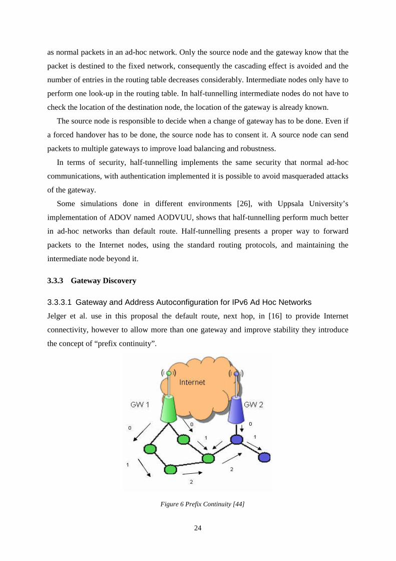
Jelger et al. use in this proposal the default route, next hop, in [16] to provide Internet
connectivity, however to allow more than one gateway and improve stability they introduce
the concept of “prefix continuity”.
Figure 6 Prefix Continuity [44]
25
To achieve prefix continuity each gateway periodically flood GW_INFO messages to its
one-hop closest neighbours, thus it is a proactive gateway discovery approach. A GW_INFO
message contains information of number of hops to the gateway and the gateway’s prefix.
This message is propagated, if the node has the same prefix as found in the GW_INFO
message. Each node updates the “number of hops to gateway” field. This scheme, with
propagating GW_INFO messages, makes nodes aware of which gateways are in the
surroundings and how many hops away they are, still avoiding to flood the entire network.
Nodes can choose to use a gateway if the number of hops to that gateway is fewer, called
”distance algorithm”, or try to use a gateway with the same prefix as long as possible , called
“stability algorithm”. As nodes chose to use a gateway, it adopts that gateways prefix; a prefix
tree will be formed with a root at the gateway.
If a proactive routing protocol is used it will also use its upstream neighbour, with the same
prefix, as default route. However, if a reactive routing protocol is used no default route will be
used; instead a gateway can answer on route request for destinations outside the MANET.
With the distance algorithm where a node always chooses the closest gateway, it will
change its prefix quite often but it will only affect few nodes, as the prefix chain is short.
If a stable prefix is preferred, the stability algorithm is used and a node tries to use the
same prefix as long as possible. However, long prefix chains can be formed, as the node will
favour upstream neighbour nodes with the same prefix.
If a change occurs in the beginning of the chain, a bulk change will occur as all
downstream neighbours also have to change their prefixes. Therefore, there is not so big
difference on the total number of prefix changes if a node use stability or distance algorithm.
However, the load-balance is improved with the distance algorithm. Nodes will be more
evenly spread between the different prefix trees, gateways, and the size variation between the
trees will be less.
A benefit of the stability algorithm is evidently that prefixes are kept longer, so the
network becomes more stable and prefix changes only occur when absolutely necessary. As
shown by simulation in [17]. Because prefix continuity, can create routes that are fragile to
changing topologies, performance is at best, as shown by simulation [33], when there is few
link breakages and low mobility. A general benefit form using [16] is that gateway
advertisements are flooded in a controlled fashion, as the messages are only propagated by
nodes with the same prefix as in the advertisement.
26
3.3.3.2 Global Connectivity for IPv6 Mobile Ad Hoc Networks
Wakikawa et al. is proposing in [37] both a proactive and reactive discovery method. With the
proactive method, unsolicited gateway advertisement messages (IGWADV) are periodically
flooded through the MANET. When using the reactive method, the gateway advertisement
message is only sent as unicast response to a gateway solicitation message (IGWSOL), sent
by a node to the ALL_MANET_GW_MULTICAST multicast address.
These messages can be implemented in two different ways [37], either as an extension to
IPv6 Neighbour Discover Protocol (NDP) or as an extension to the specific MANET routing
protocol.
From these messages a node chose a prefix to create a globally routable address and a
default route. A host based route towards the gateway is also created at the node.
When a route destination is not known a priori, (i.e. when reactive routing protocols are
used) a route request should be performed via the MANET routing protocol. If no route is
found, a node then use its default route and send the packet via either a routing header (i.e.
tunnelling) directly to the gateway or to the next hop in the default, called next hop routing.
If the gateway has a MANET local route to the destination and tunnelling has been used, it
will reply with an ICMP Redirect error message to the sender. Then the sender will perform a
new route request, to the destination, to learn the host route.
The gateway keeps a list of nodes that use its prefix for global access. This list is used for
both route examination and address management, in case of MobileIPv6. When proactive
routing protocols are used, the gateway can see which nodes are in its vicinity by checking the
topology map. If a reactive routing protocol is used, this check cannot be done, as most
reactive routing protocols do not keep the entire topology in its cache.
However, even if any method of obtaining information is allowed, all MANET nodes are
obliged to contact the gateway; at least once it establishes an internet route with the gateway.
During this contact, the gateway records them as nodes with globally routable addresses. In
the IGWADV message, there is also the possibility for the gateway to set a 1-bit
Acknowledgment flag (A). If this A flag is set, a MANET node, when it auto-configures its
address must send an Internet gateway confirmation (IGWCON) message to the gateway.
In the case of multiple gateways, in a single MANET, the associated node lists are
exchanged between the gateways, to make all gateways aware of the entire topology. The
gateways listen to routing information but preferably not participate in the normal MANET
routing, thus not forward flooded packets, like route requests, to its neighbours on the behalf
of other MANET nodes. This simplifies route examination as described in [37]. Simulation
27
[33] has shown that the performance varies heavily both under different mobility scenarios
and with different routing protocols. Although, these simulations also show that compared to
[16], the performance, of packet delivery ratio, both reactive and proactive methods scales
well with the node speed and number of link breakages. A slight performance gain could be
seen when using the proactive method; the drawback is a larger overhead because of
periodically flooding the network with IGWADV messages.
3.3.3.3 Other Approaches
In the implementation of AODV [28] done at Uppsala University, AODVUU [40], the
gateway acts as a proxy and will respond to RREQ messages that belongs in the wired part
with a special RREPI. This special message tells the nodes that all messages sent too that
address, in the wired network, should be sent via the gateway. The packets are forwarded to
the gateway by using the half-tunnelling approach described in Chapter 3.3.2.2.
In the ns2.28 implementation of DSDV [8], it is added the possibility to use next-hop
routing to reach nodes that are not inside the MANET. When nodes first are configured they
are manually assigned a gateway, so no real gateway discovery is performed. And as DSDV
is a proactive protocol, the nodes will check their routing tables and if they don’t find any
route they will send the packets to the gateway address, if that exists in the routing table
otherwise the packet is dropped.
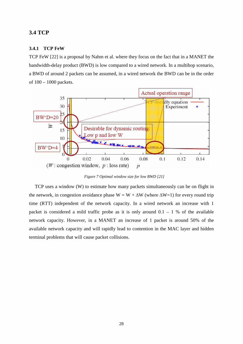
28
3.4 TCP
3.4.1 TCP FeW
TCP FeW [22] is a proposal by Nahm et al. where they focus on the fact that in a MANET the
bandwidth-delay product (BWD) is low compared to a wired network. In a multihop scenario,
a BWD of around 2 packets can be assumed, in a wired network the BWD can be in the order
of 100 – 1000 packets.
Figure 7 Optimal window size for low BWD [21]
TCP uses a window (W) to estimate how many packets simultaneously can be on flight in
the network, in congestion avoidance phase W = W + ∆W (where ∆W=1) for every round trip
time (RTT) independent of the network capacity. In a wired network an increase with 1
packet is considered a mild traffic probe as it is only around 0.1 – 1 % of the available
network capacity. However, in a MANET an increase of 1 packet is around 50% of the
available network capacity and will rapidly lead to contention in the MAC layer and hidden
terminal problems that will cause packet collisions.
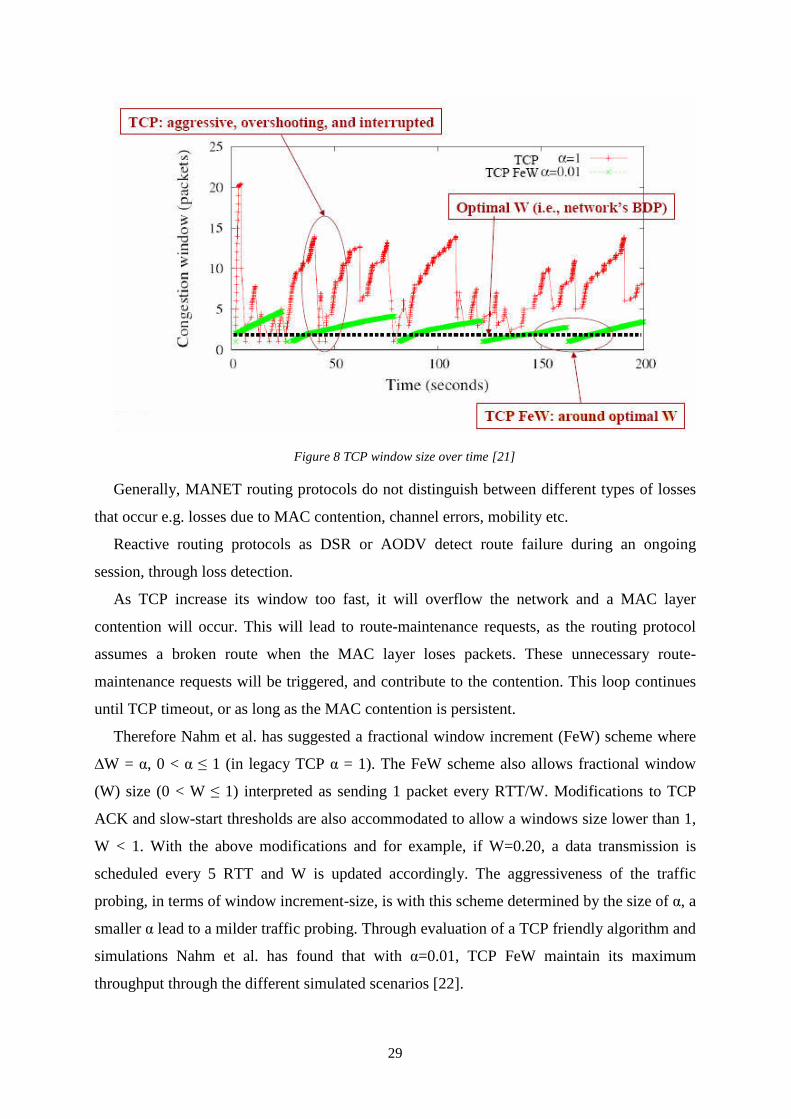
29
Figure 8 TCP window size over time [21]
Generally, MANET routing protocols do not distinguish between different types of losses
that occur e.g. losses due to MAC contention, channel errors, mobility etc.
Reactive routing protocols as DSR or AODV detect route failure during an ongoing
session, through loss detection.
As TCP increase its window too fast, it will overflow the network and a MAC layer
contention will occur. This will lead to route-maintenance requests, as the routing protocol
assumes a broken route when the MAC layer loses packets. These unnecessary route-
maintenance requests will be triggered, and contribute to the contention. This loop continues
until TCP timeout, or as long as the MAC contention is persistent.
Therefore Nahm et al. has suggested a fractional window increment (FeW) scheme where
∆W = α, 0 < α ≤ 1 (in legacy TCP α = 1). The FeW scheme also allows fractional window
(W) size (0 < W ≤ 1) interpreted as sending 1 packet every RTT/W. Modifications to TCP
ACK and slow-start thresholds are also accommodated to allow a windows size lower than 1,
W < 1. With the above modifications and for example, if W=0.20, a data transmission is
scheduled every 5 RTT and W is updated accordingly. The aggressiveness of the traffic
probing, in terms of window increment-size, is with this scheme determined by the size of α, a
smaller α lead to a milder traffic probing. Through evaluation of a TCP friendly algorithm and
simulations Nahm et al. has found that with α=0.01, TCP FeW maintain its maximum
throughput through the different simulated scenarios [22].
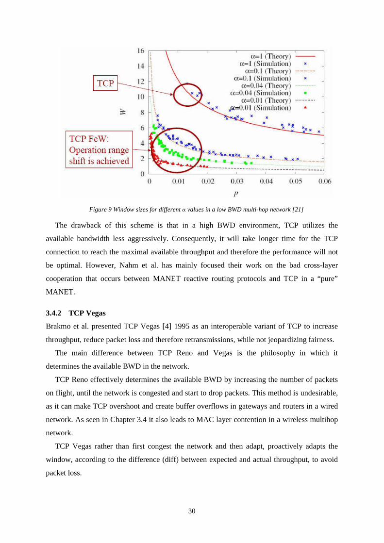
30
Figure 9 Window sizes for different α values in a low BWD multi-hop network [21]
The drawback of this scheme is that in a high BWD environment, TCP utilizes the
available bandwidth less aggressively. Consequently, it will take longer time for the TCP
connection to reach the maximal available throughput and therefore the performance will not
be optimal. However, Nahm et al. has mainly focused their work on the bad cross-layer
cooperation that occurs between MANET reactive routing protocols and TCP in a “pure”
MANET.
3.4.2 TCP Vegas
Brakmo et al. presented TCP Vegas [4] 1995 as an interoperable variant of TCP to increase
throughput, reduce packet loss and therefore retransmissions, while not jeopardizing fairness.
The main difference between TCP Reno and Vegas is the philosophy in which it
determines the available BWD in the network.
TCP Reno effectively determines the available BWD by increasing the number of packets
on flight, until the network is congested and start to drop packets. This method is undesirable,
as it can make TCP overshoot and create buffer overflows in gateways and routers in a wired
network. As seen in Chapter 3.4 it also leads to MAC layer contention in a wireless multihop
network.
TCP Vegas rather than first congest the network and then adapt, proactively adapts the
window, according to the difference (diff) between expected and actual throughput, to avoid
packet loss.
31
To achieve this proactive behaviour, Brakmo et al. proposed a scheme where W = W +
∆W. If diff < α ∆W = 1, if α < diff < β ∆W = 0 and if diff > β ∆W = -1. This difference is
calculated by diff = Threxpected - Thractual ≥ 0, where Threxpected is Current W/minimum RTT and
Thractual is the throughput calculated as how many packets sent during the time between a
packet is sent and its ACK is returned. Typically the two thresholds α and β are set between 1
and 3 in a wired network e.g. α = 1 and β = 35, in practise α = β = 26.
Modifications to the slow start behaviour and retransmission schemes are also accommodated
to avoid packet loss and unnecessary packet retransmissions.
Analytical models and simulations conducted with wired networks have shown that TCP
Vegas measures congestion by end-to-end queuing delay [19] and if the queue sizes at
intermediate nodes, routers, are large [12], TCP Vegas achieves better throughput and packet
loss ratio than TCP Reno. At the time of writing this report, no studies known to the authors,
of TCP Vegas performance has been conducted in a hybrid MANET enviroment.
In the case of inadequate queue sizes, TCP Vegas cannot utilize its improved congestion
detection mechanism and reverts to the same behaviour as TCP Reno [12]. Furthermore, [12]
shows that the higher the available bandwidth is the more efficient TCP Vegas performs.
Further studies in multihop wireless networks [7], verify that packet loss in TCP is mainly
due to MAC (IEEE802.11) layer contention, and not due to inadequate queue, buffer, sizes at
intermediate nodes.
A remark is that TCP Vegas, stated in [4] and further investigated in [19], can lead to
persistent congestion. However, the conditions that lead to persistent congestion are highly
unlikely, in a realistic scenario, as they require connections to start up serially [19]7.
The desirable aspects of TCP Vegas are:
• It is solely a modification on the sender side and therefore can interoperate with
any valid TCP implementation without modifications.
o Allows for incremental deployment
• Do not need modifications, e.g. of α and β parameters, to operate well in both
wired and wireless networks.
• Do not require explicit cross-layer notification or information.
• Reduce losses and retransmissions
5 Barkmo et al. defines that α < β to avoid fluctuations, however recent studies suggest that α = β to improve
fairness [11][19]. 6 As shown in [7] a setting of α = β = 2 also gives the best performance in a wireless multihop network. 7 Even if it is highly unlikely Low et al. propose a method to solve the problem with persistent congestion [19]
32
o Saves battery power
• Could be combined with the FeW scheme described in Chapter 3.4.1
A further enhancement that is beneficial, in a MANET, to both TCP Vegas and TCP Newreno
is ACK thinning, especially with higher bandwidths, as result of the IEEE 802.11 standard,
the cost of sending small packets, as ACKs, increase with the bandwidth [7]. However, as this
requires changing the receiver side, it does not allow incremental deployment.
Simulations [7] done by ElRakabawy et al. show that TCP Vegas α = β = 2 outperforms
TCP Newreno, especially noteworthy is that TCP Vegas achieved as much as 99% less packet
retransmissions in some of the simulated static multihop wireless network scenarios.
3.4.3 TCP AP
TCP with Adaptive Pacing is a hybrid approach that implements adaptive pacing while
retaining TCP end-to-end semantics and thus is TCP interoperable with any valid TCP
implementation [6].
The two main characteristics in this proposal is a new congestion detection and control
mechanism. Congestion detection is proactively performed by detecting link contention via
fluctuations of RTT samples. Congestion control is achieved by pacing the transmission,
based on the above measure of contention and the delay until the sender can send the next
packet, without interfering with the ongoing transmission of the former packet. This delay is
calculated by measuring RTT and by knowing available link capacity, information from the
MAC layer, and number of hops, taken from the routing layer, between the sender and the
receiver. Due to the hidden terminal effect, in a chain topology, a TCP sender at node i can
only transmit a packet successfully as soon as node (i+3) has finished its transmission. The
authors of [6] refer to the time elapsed between transmitting a TCP packet by node i and
receiving the packet at node (i+4) as the 4-hop propagation delay (FHD).
Two parameters that control the functionality are N and α. N is the number of recent RTT
samples to take into consideration and α is the averaging weight parameter in the
exponentially weighted moving average (EWMA) algorithm used to estimate the 4-hop
propagation delay.
As shown in [6], TCP AP outperforms TCP Newreno in static wireless multihop networks.
As this report focuses on hybrid MANETs the result may not be directly comparable.
The desirable aspects of TCP AP are:
• It is solely a modification on the sender side and therefore can interoperate with
any valid TCP implementation without modifications.
33
o Allows for incremental deployment
• Use the knowledge of how traffic is forwarded in multihop environments, to avoid
congesting the network.
• Reduce losses and retransmissions
o Saves battery power
The drawback is that it is not clear how the pacing mechanism works in a hybrid MANET
where there exist wired links on the path or where there only is a single wireless hop.
3.4.4 TCP with ELFN
To compensate for the disability of TCP to detect if packet loss is due to congestion or some
other reasons, Holland et al. propose a scheme with Explicit Link Failure Notification (ELFN)
[14]. The motivation to use ELFN is to avoid that TCP enter congestion avoidance in the case
of packet loss that does not originates from congestion e.g. link or route failures. The scheme
that Holland et al. propose is, when a notification comes from lower layers, TCP “freezes”
and disable its congestion control mechanism until a route is restored. In Holland et al.
proposal, retransmission timers are disabled and probe packets are sent at periodic intervals to
see if the route is re-established. When a route is re-established, TCP starts where it “left off”
when the notification occurred.
As Holland et al. shows, with mobile nodes, TCP Reno with ELFN outperforms TCP Reno
without ELFN in almost all scenarios [14].
However, as mentioned before and investigated more in [7] [22], TCP can in itself provoke
packet loss and force route changes even if there is no mobility involved.
3.4.5 A Comment on MAC Layer Unfairness
As mentioned before, in a low-bandwidth network, it is essential for TCP flow fairness that
the MAC layer is fair. Unfortunately, IEEE 802.11 MAC is not fair and this result in
disadvantageous behaviour, this is even worse when MANET local TCP flows compete with
MANET-Internet flows [25].
However, as shown in [39] with a relatively small window size (W<8), fairness is not a
problem.
3.5 Summary
In this chapter, some solutions are presented to solve the problems, already expressed in
Chapter 2, when a MANET wants to interconnect with a wired network.
34
As it is explained in Chapter 2, addressing is one of the most important problems. For this
reason to implement Mobile IP is a good solution because independently of the point that
nodes are attached, they conserve their IP address. Modification to IPv6 stateless auto-
configuration mechanism is also important, to support address configuration over multi-hop
networks, without the need for a central entity.
Three different approaches, “Gateway and Address Autoconfiguration for IPv6 Ad Hoc
Networks” [16], “Global Connectivity for IPv6 Mobile Ad Hoc Networks” [37] and
AODVUU [40], to perform gateway discovery in a MANET network are presented.
In [16], Jelger et al. use “prefix continuity”, to limit the flooding of gateway advertisement
messages. To send packets to the gateway next-hop routing is used.
Wakikawa et al. [37] is a more flexible proposal that allows both reactive and proactive
discoveries methods, to achieve a global address and to create a default path to the gateway.
To later send the packets to an internet node both next-hop routing and tunnelling are defined
in the proposal.
AODVUU use special route request reply message to inform the nodes about gateways. To
send packets to the gateway tunnelling is used.
When the route to the gateway is known, all packets that have as a destination a fixed node
have to be sent to the gateway. To facilitate this connection to the fixed network two
proposals are described to avoid continuous route discoveries, default route or next-hop
routing and half-tunnelling.
Moreover, several solutions to ease the problems with TCP’s congestion control
mechanism in MANET are proposed. As a consequence of the lack in research of how TCP
performs in hybrid MANETs, and as several of these variations mainly deal with problems in
pure MANETs, their performance can not be predicted in hybrid scenarios.
All solutions and conclusion drawn in this chapter are mostly theoretical. The following
chapter will describe some of the simulations.
4 Simulation setup
In this chapter the simulations setup, of a subset of the implementations described in Chapter
3, will be described.
35
4.1 Introduction
In this chapter some of the simulations conducted to evaluate TCP performance in a hybrid
MANET will be presented.
ns2 [41] is an open source simulator used for networking research, version 2.28 of this
simulator will be used in all the simulations.
Ns2 is not a finished product and constantly new versions come out with new protocols or
functionalities implemented. The simulator used in the simulations was extended with support
for TCP AP and AODVUU. The makefile is also changed so that the simulator compiled in
Suse Linux 9.3. This was done by installing the ns2.29 allinone package and later adding the
ns2.28 directory and changing the makefiles so ns2.28 compiled in an ns2.29 environment.
To run a simulation a Tool Command Language (TCL) script has to be written, defining
the environment for that simulation. In the script it has to be specified in detail the
characteristics of the scenario: dimensions, time of simulation, nodes, links, protocols and so
on.
To have a visual perception of the simulation there is an animation tool called Network
AniMator (NAM) that graphically shows the output file of the simulation. In NAM, nodes are
presented following the topology described in the script, time modifications can be done and
packets can be seen while they are being sent through the link. Sometimes it is hard to
distinguish packets from different nodes, for that reason some options can be used to see the
difference, as the colour or the shape. Moreover, queues can be monitored to see when and
which packets are discarded.
With the latest versions of ns2, a mobility generator is bundled, which is very useful for
huge simulations, to avoid generating all the node movements in the script.
To simplify code in wireless scenarios, some features as traffic or the mobility of the
nodes, can be defined in a separate file.
During the simulation, data can be recorded in output or trace files. It usually is difficult to
evaluate the results of the simulation looking directly at the output file. To show graphs of the
simulation results, scripts that extract data from the output files and a graph-plotting program
have to be used; one option is to use Xgraph. Another option used to visualise the results
throughout this report, is gnuplot8.
8 The bar graphs are handcrafted by inspecting trace-files and plotted with Microsoft Excel™.
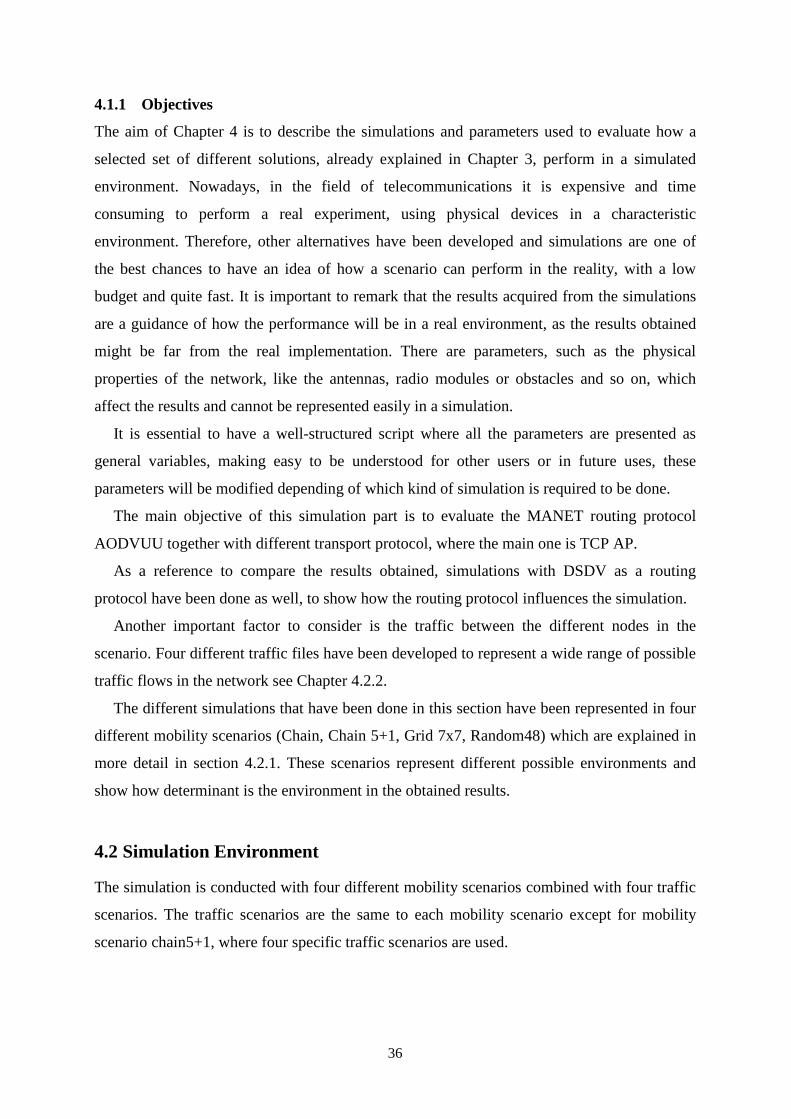
36
4.1.1 Objectives
The aim of Chapter 4 is to describe the simulations and parameters used to evaluate how a
selected set of different solutions, already explained in Chapter 3, perform in a simulated
environment. Nowadays, in the field of telecommunications it is expensive and time
consuming to perform a real experiment, using physical devices in a characteristic
environment. Therefore, other alternatives have been developed and simulations are one of
the best chances to have an idea of how a scenario can perform in the reality, with a low
budget and quite fast. It is important to remark that the results acquired from the simulations
are a guidance of how the performance will be in a real environment, as the results obtained
might be far from the real implementation. There are parameters, such as the physical
properties of the network, like the antennas, radio modules or obstacles and so on, which
affect the results and cannot be represented easily in a simulation.
It is essential to have a well-structured script where all the parameters are presented as
general variables, making easy to be understood for other users or in future uses, these
parameters will be modified depending of which kind of simulation is required to be done.
The main objective of this simulation part is to evaluate the MANET routing protocol
AODVUU together with different transport protocol, where the main one is TCP AP.
As a reference to compare the results obtained, simulations with DSDV as a routing
protocol have been done as well, to show how the routing protocol influences the simulation.
Another important factor to consider is the traffic between the different nodes in the
scenario. Four different traffic files have been developed to represent a wide range of possible
traffic flows in the network see Chapter 4.2.2.
The different simulations that have been done in this section have been represented in four
different mobility scenarios (Chain, Chain 5+1, Grid 7x7, Random48) which are explained in
more detail in section 4.2.1. These scenarios represent different possible environments and
show how determinant is the environment in the obtained results.
4.2 Simulation Environment
The simulation is conducted with four different mobility scenarios combined with four traffic
scenarios. The traffic scenarios are the same to each mobility scenario except for mobility
scenario chain5+1, where four specific traffic scenarios are used.
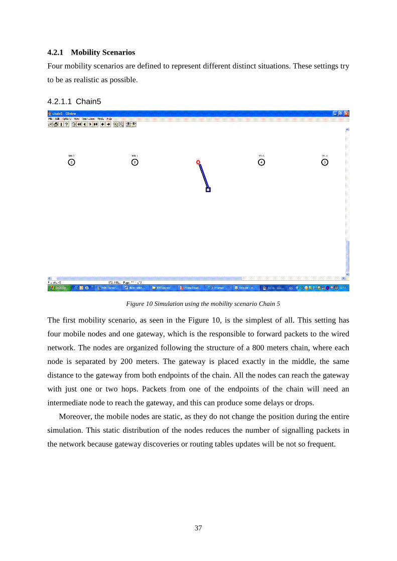
37
4.2.1 Mobility Scenarios
Four mobility scenarios are defined to represent different distinct situations. These settings try
to be as realistic as possible.
4.2.1.1 Chain5
Figure 10 Simulation using the mobility scenario Chain 5
The first mobility scenario, as seen in the Figure 10, is the simplest of all. This setting has
four mobile nodes and one gateway, which is the responsible to forward packets to the wired
network. The nodes are organized following the structure of a 800 meters chain, where each
node is separated by 200 meters. The gateway is placed exactly in the middle, the same
distance to the gateway from both endpoints of the chain. All the nodes can reach the gateway
with just one or two hops. Packets from one of the endpoints of the chain will need an
intermediate node to reach the gateway, and this can produce some delays or drops.
Moreover, the mobile nodes are static, as they do not change the position during the entire
simulation. This static distribution of the nodes reduces the number of signalling packets in
the network because gateway discoveries or routing tables updates will be not so frequent.
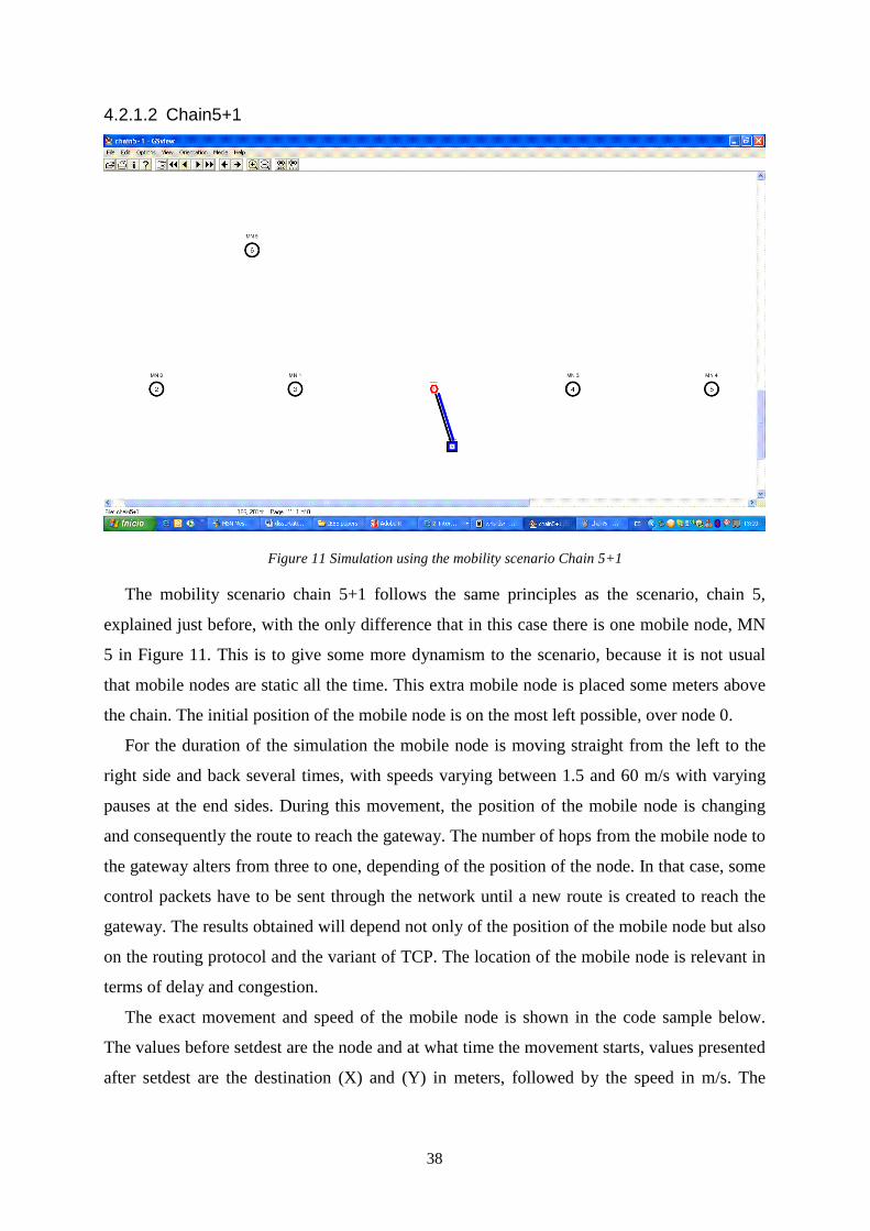
38
4.2.1.2 Chain5+1
Figure 11 Simulation using the mobility scenario Chain 5+1
The mobility scenario chain 5+1 follows the same principles as the scenario, chain 5,
explained just before, with the only difference that in this case there is one mobile node, MN
5 in Figure 11. This is to give some more dynamism to the scenario, because it is not usual
that mobile nodes are static all the time. This extra mobile node is placed some meters above
the chain. The initial position of the mobile node is on the most left possible, over node 0.
For the duration of the simulation the mobile node is moving straight from the left to the
right side and back several times, with speeds varying between 1.5 and 60 m/s with varying
pauses at the end sides. During this movement, the position of the mobile node is changing
and consequently the route to reach the gateway. The number of hops from the mobile node to
the gateway alters from three to one, depending of the position of the node. In that case, some
control packets have to be sent through the network until a new route is created to reach the
gateway. The results obtained will depend not only of the position of the mobile node but also
on the routing protocol and the variant of TCP. The location of the mobile node is relevant in
terms of delay and congestion.
The exact movement and speed of the mobile node is shown in the code sample below.
The values before setdest are the node and at what time the movement starts, values presented
after setdest are the destination (X) and (Y) in meters, followed by the speed in m/s. The
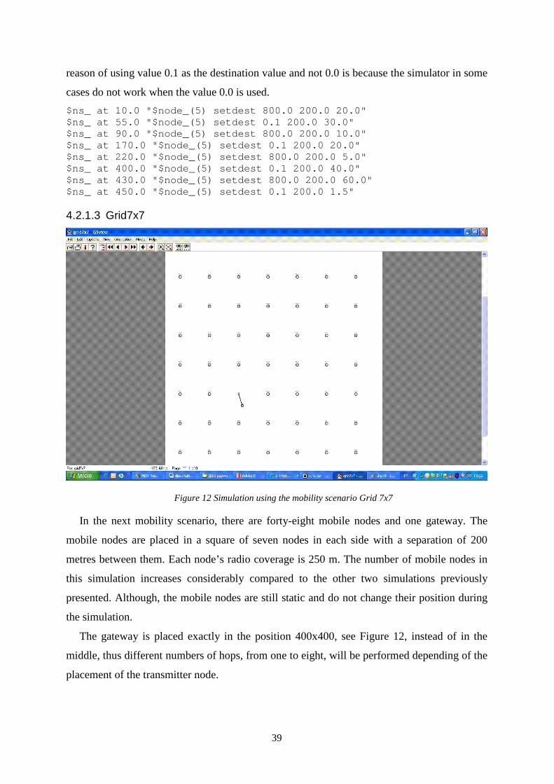
39
reason of using value 0.1 as the destination value and not 0.0 is because the simulator in some
cases do not work when the value 0.0 is used.
$ns_ at 10.0 "$node_(5) setdest 800.0 200.0 20.0" $ns_ at 55.0 "$node_(5) setdest 0.1 200.0 30.0" $ns_ at 90.0 "$node_(5) setdest 800.0 200.0 10.0" $ns_ at 170.0 "$node_(5) setdest 0.1 200.0 20.0" $ns_ at 220.0 "$node_(5) setdest 800.0 200.0 5.0" $ns_ at 400.0 "$node_(5) setdest 0.1 200.0 40.0" $ns_ at 430.0 "$node_(5) setdest 800.0 200.0 60.0" $ns_ at 450.0 "$node_(5) setdest 0.1 200.0 1.5"
4.2.1.3 Grid7x7
Figure 12 Simulation using the mobility scenario Grid 7x7
In the next mobility scenario, there are forty-eight mobile nodes and one gateway. The
mobile nodes are placed in a square of seven nodes in each side with a separation of 200
metres between them. Each node’s radio coverage is 250 m. The number of mobile nodes in
this simulation increases considerably compared to the other two simulations previously
presented. Although, the mobile nodes are still static and do not change their position during
the simulation.
The gateway is placed exactly in the position 400x400, see Figure 12, instead of in the
middle, thus different numbers of hops, from one to eight, will be performed depending of the
placement of the transmitter node.
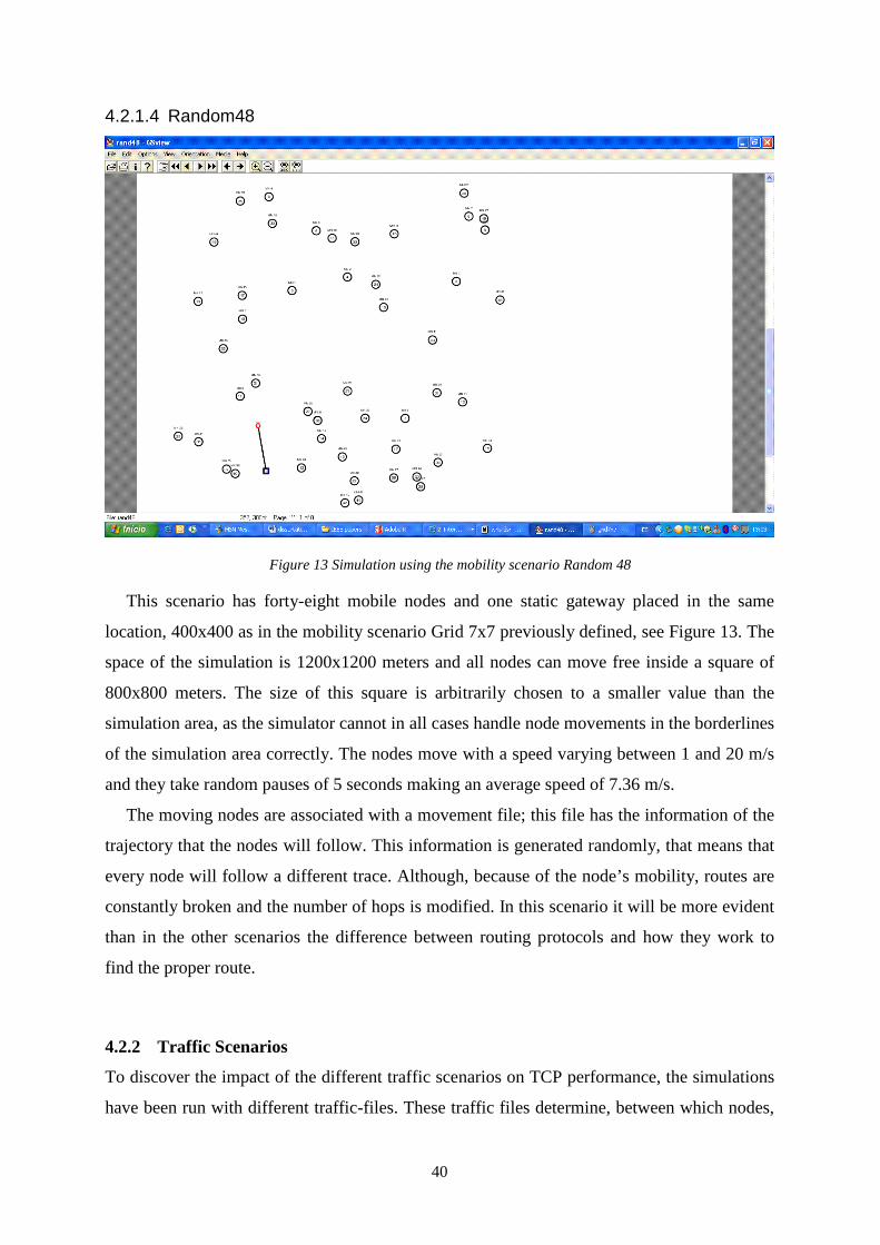
40
4.2.1.4 Random48
Figure 13 Simulation using the mobility scenario Random 48
This scenario has forty-eight mobile nodes and one static gateway placed in the same
location, 400x400 as in the mobility scenario Grid 7x7 previously defined, see Figure 13. The
space of the simulation is 1200x1200 meters and all nodes can move free inside a square of
800x800 meters. The size of this square is arbitrarily chosen to a smaller value than the
simulation area, as the simulator cannot in all cases handle node movements in the borderlines
of the simulation area correctly. The nodes move with a speed varying between 1 and 20 m/s
and they take random pauses of 5 seconds making an average speed of 7.36 m/s.
The moving nodes are associated with a movement file; this file has the information of the
trajectory that the nodes will follow. This information is generated randomly, that means that
every node will follow a different trace. Although, because of the node’s mobility, routes are
constantly broken and the number of hops is modified. In this scenario it will be more evident
than in the other scenarios the difference between routing protocols and how they work to
find the proper route.
4.2.2 Traffic Scenarios
To discover the impact of the different traffic scenarios on TCP performance, the simulations
have been run with different traffic-files. These traffic files determine, between which nodes,
41
which kind of and when the traffic-flows start and stop. The traffic flows try to simulate a
scenario where one or two MANET node(s) are uploading file(s) to a wired host, so the traffic
is always originating from the MANET and directed towards the wired network. The flow-
delay is a parameter that decides how much time should pass until the traffic flow starts and
how long time before the end of the simulation the traffic should stop. This is to be able to
better show the resulting traffic flow in a graph, if not used the last ACK packets would be
after that the simulation ends and invisible in the graphs, see Appendix B.
We have selected different traffic scenarios to cover as many typical traffic situations as
possible.
Default values for all traffic files unless stated otherwise:
• Type of traffic FTP, simulating a large file transfer
• Transport Layer Agent TCP (TCP variants see Chapter 4.3)
• Flow(s) 1 or 2
o Identification 1 for first flow and 2 for second flow
o Start
� Flow 1 1 & 2 flows, start of simulation + flow-delay (20)
� Flow 2 (end of simulation– flow-delay)/4 (220)
o Stop
� Flow 1 if 1 flow, (end of simulation-flow-delay) (880)
if 2 flows, (end of simulation-flow-delay)/2 (440)
� Flow 2 end of simulation – flow-delay (880)
For each mobility scenario, Chain5, Grid7x7 and Random48, there are 4 different traffic
files.
In all traffic files, unless otherwise stated, the source node of the flow crossing
MANET/Internet border is denoted as node 0 and the destination is the Wired Host.
1_tcp-from_node_0
One FTP flow from the MANET to the wired network.
1-tcp-from-node-0-1-tcp-between-node-4-node-0
Two FTP flows, one from the MANET to the wired network and another one
within the MANET, between Mobile Node 0 and Mobile Node 4.
2-tcp-from-node-0-node-4-simultaneous
Two FTP flows, from the MANET, Mobile Node 0 and Mobile Node 4, to the
wired network both starting and stopping at the same time. They start at: 20 and
stop at 880.
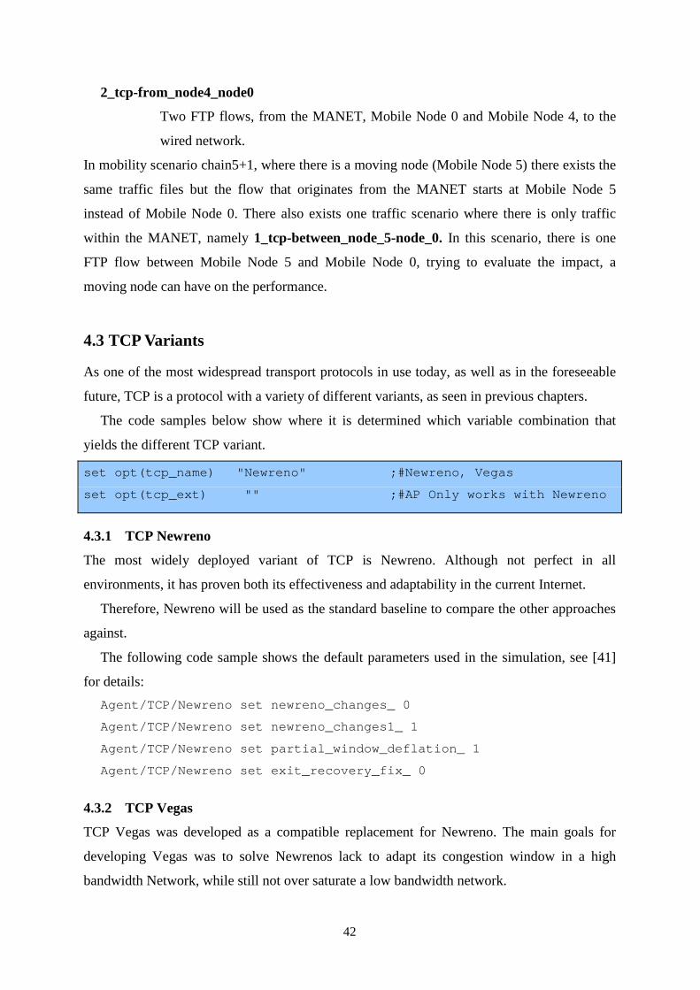
42
2_tcp-from_node4_node0
Two FTP flows, from the MANET, Mobile Node 0 and Mobile Node 4, to the
wired network.
In mobility scenario chain5+1, where there is a moving node (Mobile Node 5) there exists the
same traffic files but the flow that originates from the MANET starts at Mobile Node 5
instead of Mobile Node 0. There also exists one traffic scenario where there is only traffic
within the MANET, namely 1_tcp-between_node_5-node_0. In this scenario, there is one
FTP flow between Mobile Node 5 and Mobile Node 0, trying to evaluate the impact, a
moving node can have on the performance.
4.3 TCP Variants
As one of the most widespread transport protocols in use today, as well as in the foreseeable
future, TCP is a protocol with a variety of different variants, as seen in previous chapters.
The code samples below show where it is determined which variable combination that
yields the different TCP variant.
set opt(tcp_name) "Newreno" ;#Newreno, Vegas
set opt(tcp_ext) "" ;#AP Only works with Newreno
4.3.1 TCP Newreno
The most widely deployed variant of TCP is Newreno. Although not perfect in all
environments, it has proven both its effectiveness and adaptability in the current Internet.
Therefore, Newreno will be used as the standard baseline to compare the other approaches
against.
The following code sample shows the default parameters used in the simulation, see [41]
for details:
Agent/TCP/Newreno set newreno_changes_ 0
Agent/TCP/Newreno set newreno_changes1_ 1
Agent/TCP/Newreno set partial_window_deflation_ 1
Agent/TCP/Newreno set exit_recovery_fix_ 0
4.3.2 TCP Vegas
TCP Vegas was developed as a compatible replacement for Newreno. The main goals for
developing Vegas was to solve Newrenos lack to adapt its congestion window in a high
bandwidth Network, while still not over saturate a low bandwidth network.
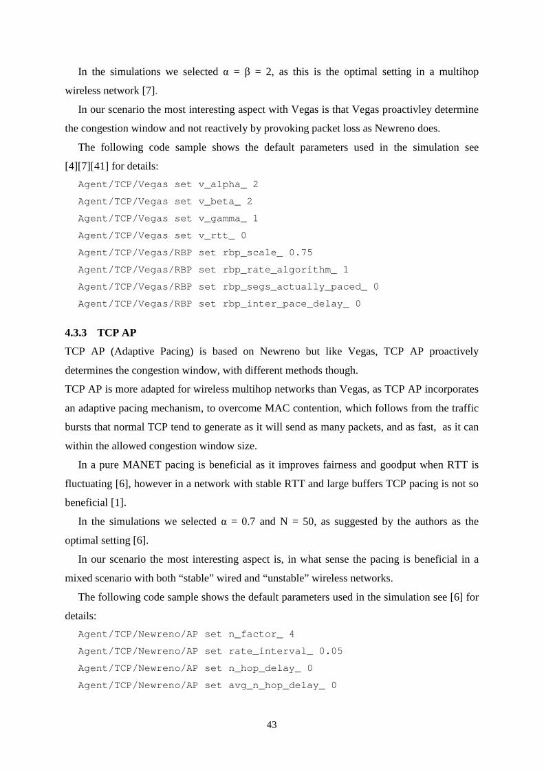
43
In the simulations we selected α = β = 2, as this is the optimal setting in a multihop
wireless network [7].
In our scenario the most interesting aspect with Vegas is that Vegas proactivley determine
the congestion window and not reactively by provoking packet loss as Newreno does.
The following code sample shows the default parameters used in the simulation see
[4] [7] [41] for details:
Agent/TCP/Vegas set v_alpha_ 2
Agent/TCP/Vegas set v_beta_ 2
Agent/TCP/Vegas set v_gamma_ 1
Agent/TCP/Vegas set v_rtt_ 0
Agent/TCP/Vegas/RBP set rbp_scale_ 0.75
Agent/TCP/Vegas/RBP set rbp_rate_algorithm_ 1
Agent/TCP/Vegas/RBP set rbp_segs_actually_paced_ 0
Agent/TCP/Vegas/RBP set rbp_inter_pace_delay_ 0
4.3.3 TCP AP
TCP AP (Adaptive Pacing) is based on Newreno but like Vegas, TCP AP proactively
determines the congestion window, with different methods though.
TCP AP is more adapted for wireless multihop networks than Vegas, as TCP AP incorporates
an adaptive pacing mechanism, to overcome MAC contention, which follows from the traffic
bursts that normal TCP tend to generate as it will send as many packets, and as fast, as it can
within the allowed congestion window size.
In a pure MANET pacing is beneficial as it improves fairness and goodput when RTT is
fluctuating [6], however in a network with stable RTT and large buffers TCP pacing is not so
beneficial [1].
In the simulations we selected α = 0.7 and N = 50, as suggested by the authors as the
optimal setting [6].
In our scenario the most interesting aspect is, in what sense the pacing is beneficial in a
mixed scenario with both “stable” wired and “unstable” wireless networks.
The following code sample shows the default parameters used in the simulation see [6] for
details:
Agent/TCP/Newreno/AP set n_factor_ 4
Agent/TCP/Newreno/AP set rate_interval_ 0.05
Agent/TCP/Newreno/AP set n_hop_delay_ 0
Agent/TCP/Newreno/AP set avg_n_hop_delay_ 0
44
Agent/TCP/Newreno/AP set coeff_var_ 0
Agent/TCP/Newreno/AP set adev_ 0
Agent/TCP/Newreno/AP set history_ 50
Agent/TCP/Newreno/AP set delaybound_ 0.5
Agent/TCP/Newreno/AP set alpha_ 0.7
Agent/TCP/Newreno/AP set ll_bandwidth_ 2e6
4.4 Routing and Gateway Discovery
AODVUU and DSDV are the routing protocols used in all the simulations. The one evaluated
in detail is however AODVUU. DSDV is included for the interested as a reference, to see the
difference a proactive routing protocol with gateway and next-hop routing support has on
performance. The DSDV used is the version that comes with ns2.28.
4.4.1 AODVUU
#Wireless
set opt(rp) AODVUU ;# DSDV, AODVUU
AODVUU is version 0.91 of the implementation of AODV by Uppsala University, as a
reactive routing protocol with added functionality for gateway discovery and half tunnelling
capabilities.
The following code sample shows the default parameters for mobile nodes used in the
simulation, see AODVUU in [40] for details:
Agent/AODVUU set expanding_ring_search_ 1 ;#for RRE Qs
Agent/AODVUU set ratelimit_ 1 ;#rate limiting for R REQs and RERRs
Agent/AODVUU set llfeedback_ 1 ;# use link layer
Agent/AODVUU set internet_gw_mode_ 0 ;#1 = gateway node
Agent/AODVUU set unidir_hack_ 0
Agent/AODVUU set rreq_gratuitous_ 0
Agent/AODVUU set local_repair_ 0
Agent/AODVUU set receive_n_hellos_ 0
Agent/AODVUU set hello_jittering_ 0
Agent/AODVUU set wait_on_reboot_ 0
Agent/AODVUU set debug_ 0
Agent/AODVUU set rt_log_interval_ 0
Agent/AODVUU set log_to_file_ 0
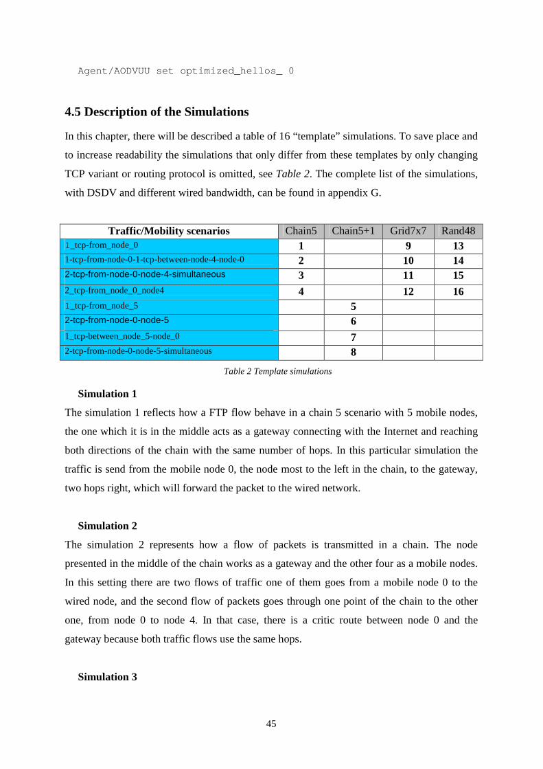
45
Agent/AODVUU set optimized_hellos_ 0
4.5 Description of the Simulations
In this chapter, there will be described a table of 16 “template” simulations. To save place and
to increase readability the simulations that only differ from these templates by only changing
TCP variant or routing protocol is omitted, see Table 2. The complete list of the simulations,
with DSDV and different wired bandwidth, can be found in appendix G.
Traffic/Mobility scenarios Chain5 Chain5+1 Grid7x7 Rand48 1_tcp-from_node_0 1 9 13 1-tcp-from-node-0-1-tcp-between-node-4-node-0 2 10 14 2-tcp-from-node-0-node-4-simultaneous 3 11 15 2_tcp-from_node_0_node4 4 12 16 1_tcp-from_node_5 5 2-tcp-from-node-0-node-5 6 1_tcp-between_node_5-node_0 7 2-tcp-from-node-0-node-5-simultaneous 8
Table 2 Template simulations
Simulation 1
The simulation 1 reflects how a FTP flow behave in a chain 5 scenario with 5 mobile nodes,
the one which it is in the middle acts as a gateway connecting with the Internet and reaching
both directions of the chain with the same number of hops. In this particular simulation the
traffic is send from the mobile node 0, the node most to the left in the chain, to the gateway,
two hops right, which will forward the packet to the wired network.
Simulation 2
The simulation 2 represents how a flow of packets is transmitted in a chain. The node
presented in the middle of the chain works as a gateway and the other four as a mobile nodes.
In this setting there are two flows of traffic one of them goes from a mobile node 0 to the
wired node, and the second flow of packets goes through one point of the chain to the other
one, from node 0 to node 4. In that case, there is a critic route between node 0 and the
gateway because both traffic flows use the same hops.
Simulation 3
46
The simulation 3 reflects how packets sent in a FTP flow. In that case there are two different
flows both of them to the wired node but with different sources each point of the chain node 0
and node 4. Do not share hops because they use two paths completely different. The gateway
is the only point in common for these two traces. Both flows start and stop at the same time,
to be able to determine the fairness between the both flows.
Simulation 4
In that case, simulation 4 is very similar to the previous simulation number 3 because the
involved nodes are exactly the same, node 0, node 4 and a wired node. The main difference in
this simulation is that the both flows do not start at the same time. This is to evaluate if there
is a difference if both flows start simultaneous or if they start at an arbitrary point.
Simulation 5
As is explained before chain5+1 is an extension of chain 5, for this reason special traffic files
are used, where the extra mobile node is involved. Simulation 5 is the first one using chain
5+1 as a scenario. In this particular case, the traffic file goes from the mobile node 5 to the
wired host. During the simulation node 5 is attached to different mobile nodes in the chain
and therefore the number of hops is changing constantly. Each time that the node is attached
to a new intermediate node it has to do a gateway discovery to reach the wired host.
Simulation 6
This simulation is similar to simulation 4, the difference is that one of the flows comes from
the moving node, mobile node 5.
Simulation 7
At the beginning of the simulation node 5 will have direct connection with the destination
because it will be one hop to the source. However, during the simulation the node will move
between the extreme ends of the chain. So it will be between 1 and 5 hops to the destination.
In this simulation it can be observed how important the number of hops between source and
receiver is for the delay.
Simulation 8
This simulation is similar to simulation 3. The difference is that one of the flows comes from
(the) moving node, mobile node 5.
47
Simulation 9
In this simulation, we evaluate throughput in a static grid, representing fixed rely stations and
stationary desktop computers uploading a large file to a wired host. The traffic is sent from
mobile node 0 to the wired host, the number of hops between the gateway and the mobile
node is at least 4.
Simulation 10
In this simulation, it is evaluated the performance of two competing FTP streams in a static
grid, representing fixed rely stations and stationary desktops computers where one node is
uploading a file to a wired host while communicating with another node in the grid.
Simulation 11
In this simulation, it is evaluated the fairness and performance between two competing FTP
streams in a static grid, representing fixed rely stations and stationary desktops computers
uploading large files to a wired host.
Simulation 12
In this simulation, it is evaluated the performance of two competing FTP streams in a static
grid, representing fixed rely stations and stationary desktops computers uploading large files
to a wired server, where both flows don’t start at the same time.
Simulation 13
In this simulation, it is evaluated the performance in a scenario where the 48 nodes move
freely in an 800x800m area at speeds varying between 1 and 20 m/s with 5 seconds pause,
representing nodes at walking or driving speed, where one node is uploading a large file to a
wired host.
Simulation 14
In this simulation, it is evaluated the performance between two competing FTP streams in a
scenario where the 48 nodes move freely in an 800x800m area at speeds varying between 1 an
20 m/s with 5 seconds pause, representing nodes at walking or driving speed where one node
is uploading a file to a wired host while starting a download from another MANET node.
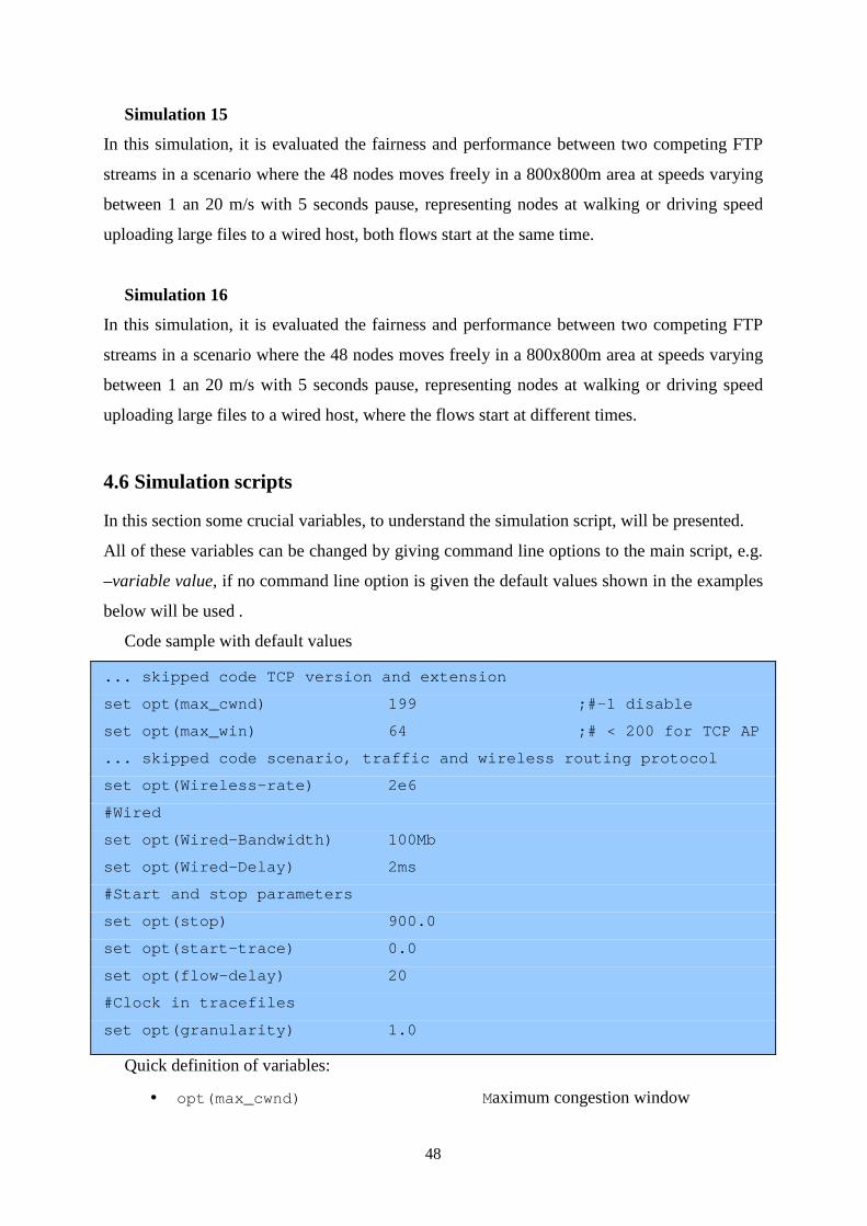
48
Simulation 15
In this simulation, it is evaluated the fairness and performance between two competing FTP
streams in a scenario where the 48 nodes moves freely in a 800x800m area at speeds varying
between 1 an 20 m/s with 5 seconds pause, representing nodes at walking or driving speed
uploading large files to a wired host, both flows start at the same time.
Simulation 16
In this simulation, it is evaluated the fairness and performance between two competing FTP
streams in a scenario where the 48 nodes moves freely in a 800x800m area at speeds varying
between 1 an 20 m/s with 5 seconds pause, representing nodes at walking or driving speed
uploading large files to a wired host, where the flows start at different times.
4.6 Simulation scripts
In this section some crucial variables, to understand the simulation script, will be presented.
All of these variables can be changed by giving command line options to the main script, e.g.
–variable value, if no command line option is given the default values shown in the examples
below will be used .
Code sample with default values
... skipped code TCP version and extension
set opt(max_cwnd) 199 ;#-1 disable
set opt(max_win) 64 ;# < 200 for TCP AP
... skipped code scenario, traffic and wireless rou ting protocol
set opt(Wireless-rate) 2e6
#Wired
set opt(Wired-Bandwidth) 100Mb
set opt(Wired-Delay) 2ms
#Start and stop parameters
set opt(stop) 900.0
set opt(start-trace) 0.0
set opt(flow-delay) 20
#Clock in tracefiles
set opt(granularity) 1.0
Quick definition of variables:
• opt(max_cwnd) M aximum congestion window

49
in number of packets, -1 disable
• opt(max_win) M aximum Advertised window
in number of packets, -1 disable
• opt(Wireless-rate) Physical bandwidth wireless in bits
• opt(Wired-Bandwidth) Physical bandwidth wired Mbits
• opt(Wired-Delay) Delay on wired link in milliseconds
• opt(stop) Simulation time in seconds
• opt(start-trace) Time to start trace in seconds
• opt(granularity) Time between trace probes in seconds
• opt(flow-delay) see Chapter 4.2.2
4.6.1 Traces
The following parameters will be traced during all simulations:
• Congestion window in number of packets of sending node(s)
• Throughput and Goodput in Kbit/s measured at the sending node(s)
• Throughput and Goodput in Packets/s measured at the sending node(s)
• In the case of 2 streams, fairness in terms of “Jain’s Fairness” index [15].
4.6.2 Formulas
Formulas:
• Goodput (KBits/s)= 1000
8
)(
)(Re)( ×−stime
bytesdbytestransmittebytesdbytesTransmitte
• Jain’s Fairness Index =
×
∑
∑n
i
n
i
Xn
X
1
2
2
1
o n is the number of flows and Xi is the throughput of the i:th flow, see [15] for
details.
4.6.3 Running the Simulation and Post Processing
There are two post processing scripts, postprocess.pl and afterburner.pl. The former processes
the trace files into a format that gnuplot can use to produce graphs. The latter is used to
collect data from different simulations to combine them into one graph.
Running the simulation

50
To reproduce the simulations used in this thesis there is a small helper script called
simulations.pl that feed the main script with correct command line options.
To run all simulations, the command line to use is “perl simulations.pl all”. This will run all
the simulations with a wired bandwidth of 100 Mb and 2ms delay, to run the simulation with
different bandwidth and delay the command line is “perl simulations.pl all –Wired-
Bandwidth 756Kb -Wired-Delay 25ms ”. , If only a subset of the simulations should be run,
the exact simulations must be specified like “perl simulations.pl 1 6 100” for simulations 1, 6
and 100. To remember is that the simulation number, given on the command line, is not the
template simulation number in Chapter 4.5, the simulation number is the one stated in
appendix G.3.
4.7 Summary
In this chapter, the different parts and parameters of the simulation setup are described to
easier understand and clarify Chapter 5. This chapter can also be used as a reference and
overview of the complete code that can be found in appendix D.
Later in Chapter 5, some of the different “template” simulations will be used to evaluate and
visualise the results obtained from all of the simulations found in appendix G.4.
All of the above described simulations are conducted with AODVUU and DSDV
combined with TCP Vegas, TCP Newreno and TCP AP. All of these simulations were
thereafter run one time with a wired bandwidth of 100Mb and a delay of 2ms and one time
with a wired bandwidth of 756KB and a delay of 25ms.
5 Evaluation of Simulations
In this chapter results from some of the simulations, described in Chapter 4, will be presented
and evaluated.
5.1 Introduction
Chapter 4 describes all the parameters for the simulation setup. It is important to have a
previous knowledge about what will be simulated to understand correctly the results obtained
in this chapter. Using the script attached in the appendix D.2 around a couple of hundred
simulations have been run. With all this information, it is difficult to go into detail about
51
every simulation run, so this chapter can be seen as an overview, where some simulations are
highlighted to give a more clear view, on which parameters are influent in the situation.
In this chapter we consider it decisive to present in a graphically way the results acquired
from the simulations.
So, to save space and to increase the readability only the simulations 1, 5, 9 and 13 are
presented, as these are the simulations where the difference in traffic is most clear.
However, all the graphs from the simulations are found in appendix G.4 Each graph is
representing a specific simulation with all three TCP variants, Newreno, Vegas and TCP AP
(Newreno AP).
In all simulations, the congestion window is limited to 199 packets, as this is the default
limit for TCP AP. Even though this limit is set in the simulator, as seen in the grid scenario,
this limit is exceeded and TCP AP fails. The advertised window is set to 64 packets.
The simulation is conducted as a comparison between three TCP variants, TCP Newreno,
TCP Vegas and TCP AP, and two different routing protocols, AODVUU and DSDV.
In the main simulation setup the wired bandwidth is set to 100Mb with a delay of 2ms to
represent a local LAN. Additionally as a small comparison, a second simulation run is
conducted with a wired bandwidth of 756Kb and 25ms, delay representing a typical Internet
connection.
5.2 Performance parameters
The following performance parameters are evaluated in more detail: congestion window,
throughput and goodput.
For each simulation that we present there are five graphs representing congestion window,
throughput, goodput, aggregate of throughput and congestion window. For reference there is
also included one graph representing the aggregate throughput when using DSDV.
Congestion window is measured at the sender as number of packets allowed on flight in the
network.
Throughput is measured at the sender as number of Kbits sent per second.
Goodput is measured at the sender as number of Kbits sent - number of Kbits resent per
second.
Fairness is calculated based Jain’s fairness index over the flows that run in parallel.
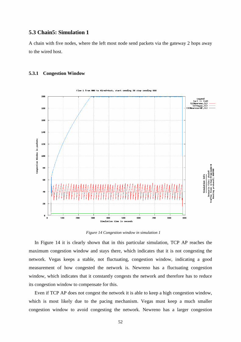
52
5.3 Chain5: Simulation 1
A chain with five nodes, where the left most node send packets via the gateway 2 hops away
to the wired host.
5.3.1 Congestion Window
Figure 14 Congestion window in simulation 1
In Figure 14 it is clearly shown that in this particular simulation, TCP AP reaches the
maximum congestion window and stays there, which indicates that it is not congesting the
network. Vegas keeps a stable, not fluctuating, congestion window, indicating a good
measurement of how congested the network is. Newreno has a fluctuating congestion
window, which indicates that it constantly congests the network and therefore has to reduce
its congestion window to compensate for this.
Even if TCP AP does not congest the network it is able to keep a high congestion window,
which is most likely due to the pacing mechanism. Vegas must keep a much smaller
congestion window to avoid congesting the network. Newreno has a larger congestion
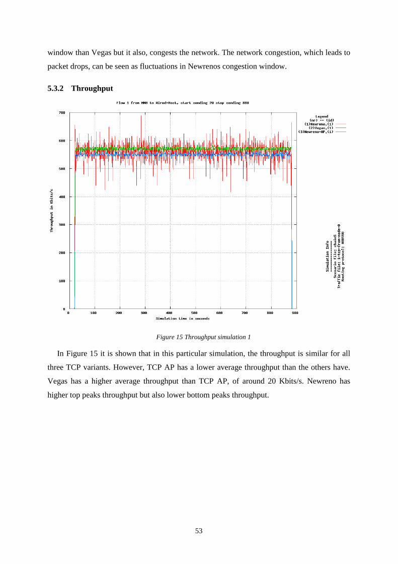
53
window than Vegas but it also, congests the network. The network congestion, which leads to
packet drops, can be seen as fluctuations in Newrenos congestion window.
5.3.2 Throughput
Figure 15 Throughput simulation 1
In Figure 15 it is shown that in this particular simulation, the throughput is similar for all
three TCP variants. However, TCP AP has a lower average throughput than the others have.
Vegas has a higher average throughput than TCP AP, of around 20 Kbits/s. Newreno has
higher top peaks throughput but also lower bottom peaks throughput.
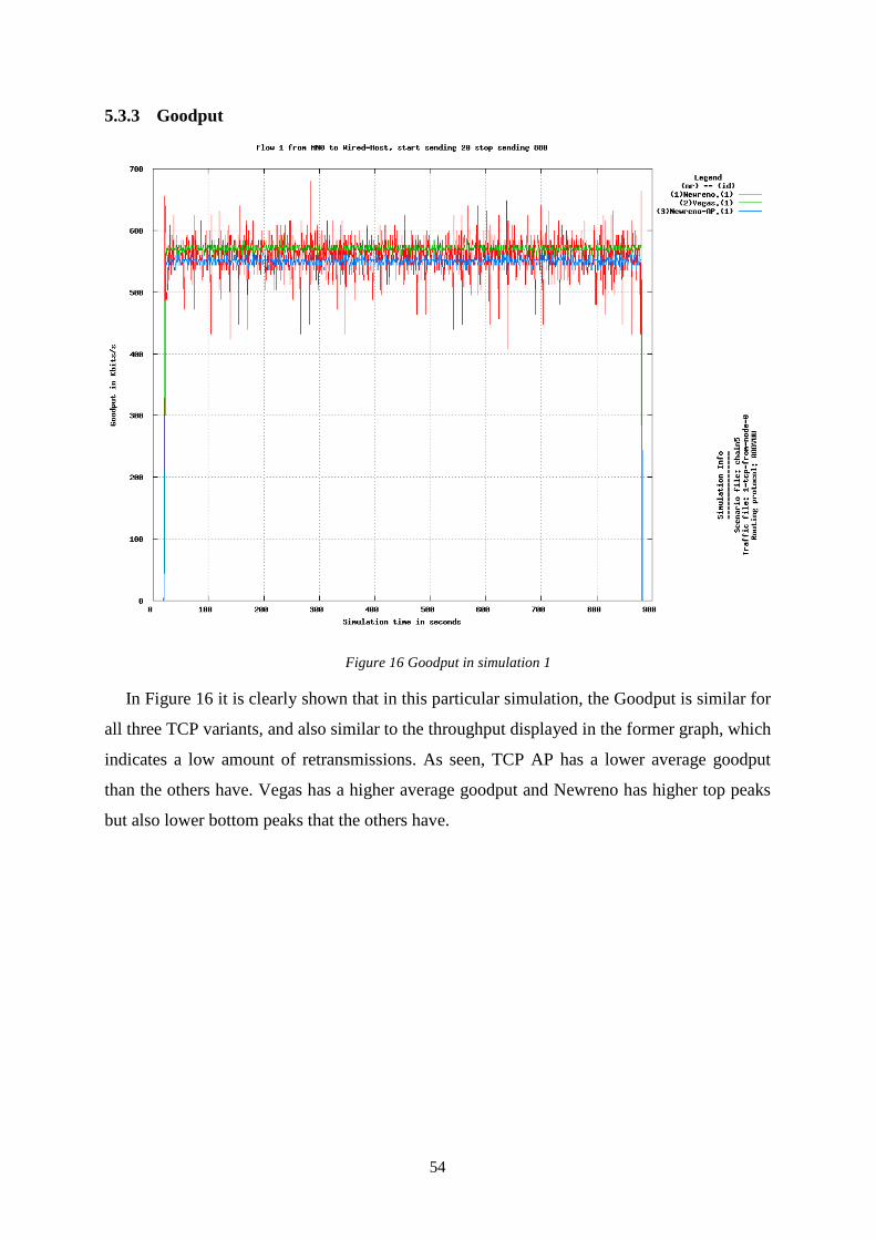
54
5.3.3 Goodput
Figure 16 Goodput in simulation 1
In Figure 16 it is clearly shown that in this particular simulation, the Goodput is similar for
all three TCP variants, and also similar to the throughput displayed in the former graph, which
indicates a low amount of retransmissions. As seen, TCP AP has a lower average goodput
than the others have. Vegas has a higher average goodput and Newreno has higher top peaks
but also lower bottom peaks that the others have.
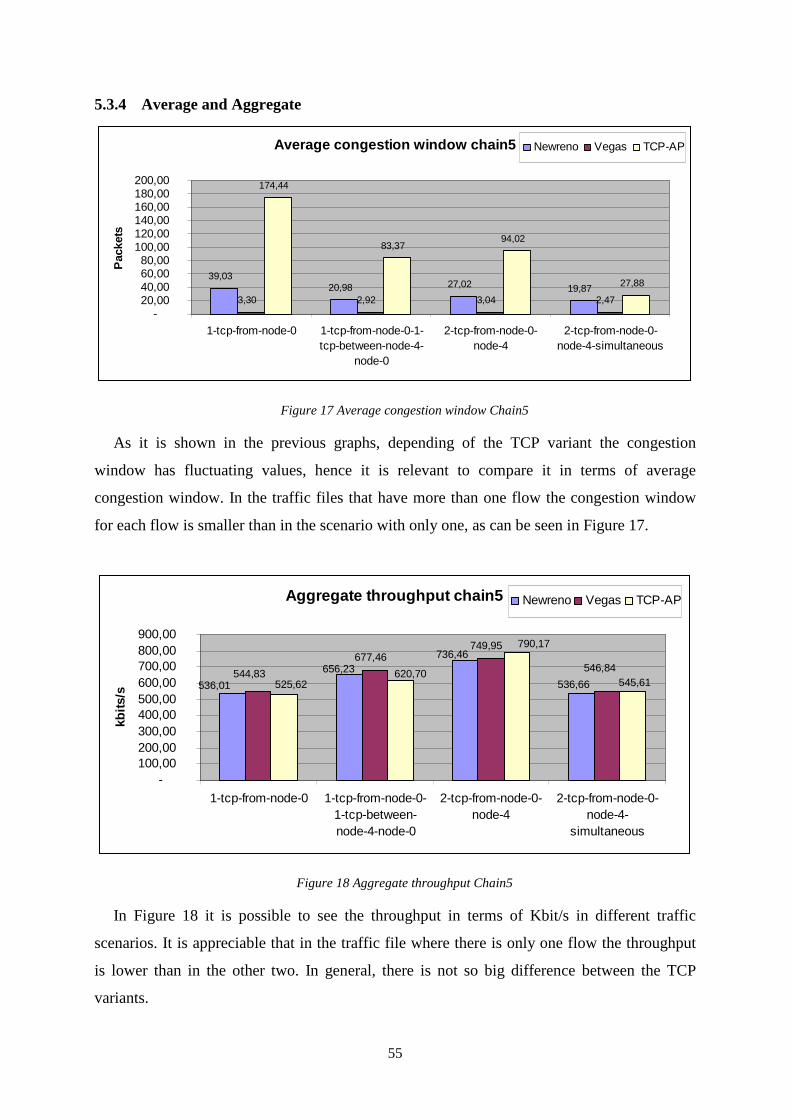
55
5.3.4 Average and Aggregate
Average congestion window chain5
39,03 20,98 27,02 19,87
3,30 2,92 3,04 2,47
174,44
83,37 94,02
27,88
- 20,00 40,00 60,00 80,00
100,00 120,00 140,00 160,00 180,00 200,00
1-tcp-from-node-0 1-tcp-from-node-0-1-tcp-between-node-4-
node-0
2-tcp-from-node-0-node-4
2-tcp-from-node-0-node-4-simultaneous
Pac
kets
Newreno Vegas TCP-AP
Figure 17 Average congestion window Chain5
As it is shown in the previous graphs, depending of the TCP variant the congestion
window has fluctuating values, hence it is relevant to compare it in terms of average
congestion window. In the traffic files that have more than one flow the congestion window
for each flow is smaller than in the scenario with only one, as can be seen in Figure 17.
Aggregate throughput chain5
677,46 749,95
536,66
736,46 656,23
536,01
546,84 544,83 545,61
790,17
620,70 525,62
- 100,00 200,00 300,00 400,00 500,00 600,00 700,00 800,00 900,00
1-tcp-from-node-0 1-tcp-from-node-0-1-tcp-between-node-4-node-0
2-tcp-from-node-0-node-4
2-tcp-from-node-0-node-4-
simultaneous
kbits
/s
Newreno Vegas TCP-AP
Figure 18 Aggregate throughput Chain5
In Figure 18 it is possible to see the throughput in terms of Kbit/s in different traffic
scenarios. It is appreciable that in the traffic file where there is only one flow the throughput
is lower than in the other two. In general, there is not so big difference between the TCP
variants.
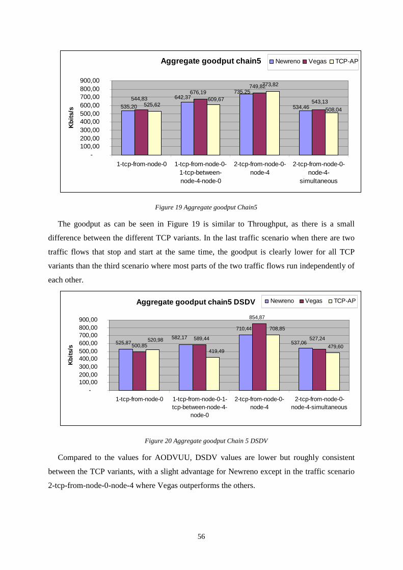
56
Aggregate goodput chain5
676,19 749,82
525,62 534,46
735,25 642,37
535,20 543,13 544,83
773,82
609,67
508,04
- 100,00 200,00 300,00 400,00 500,00 600,00 700,00 800,00 900,00
1-tcp-from-node-0 1-tcp-from-node-0-1-tcp-between-node-4-node-0
2-tcp-from-node-0-node-4
2-tcp-from-node-0-node-4-
simultaneous
Kbi
ts/s
Newreno Vegas TCP-AP
Figure 19 Aggregate goodput Chain5
The goodput as can be seen in Figure 19 is similar to Throughput, as there is a small
difference between the different TCP variants. In the last traffic scenario when there are two
traffic flows that stop and start at the same time, the goodput is clearly lower for all TCP
variants than the third scenario where most parts of the two traffic flows run independently of
each other.
Aggregate goodput chain5 DSDV
525,87
710,44
854,87
537,06 582,17 527,24 589,44
500,85 479,60
708,85
419,49
520,98
- 100,00 200,00 300,00 400,00 500,00 600,00 700,00 800,00 900,00
1-tcp-from-node-0 1-tcp-from-node-0-1-tcp-between-node-4-
node-0
2-tcp-from-node-0-node-4
2-tcp-from-node-0-node-4-simultaneous
Kbi
ts/s
Newreno Vegas TCP-AP
Figure 20 Aggregate goodput Chain 5 DSDV
Compared to the values for AODVUU, DSDV values are lower but roughly consistent
between the TCP variants, with a slight advantage for Newreno except in the traffic scenario
2-tcp-from-node-0-node-4 where Vegas outperforms the others.
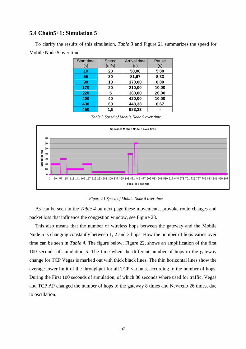
57
5.4 Chain5+1: Simulation 5
To clarify the results of this simulation, Table 3and Figure 21 summarizes the speed for
Mobile Node 5 over time.
Start time (s)
Speed (m/s)
Arrival time (s)
Pause (s)
10 20 50,00 5,00 55 30 81,67 8,33 90 10 170,00 0,00 170 20 210,00 10,00 220 5 380,00 20,00 400 40 420,00 10,00 430 60 443,33 6,67 450 1,5 983,33 -
Table 3 Speed of Mobile Node 5 over time
Spe ed of M obile Node 5 ove r tim e
0
10
20
30
40
50
60
70
1 29 57 85 113 141 169 197 225 253 281 309 337 365 393 421 449 477 505 533 561 589 617 645 673 701 729 757 785 813 841 869 897
Tim e in Se conds
Spe
ed in
m/s
Figure 21 Speed of Mobile Node 5 over time
As can be seen in the Table 4 on next page these movements, provoke route changes and
packet loss that influence the congestion window, see Figure 23.
This also means that the number of wireless hops between the gateway and the Mobile
Node 5 is changing constantly between 1, 2 and 3 hops. How the number of hops varies over
time can be seen in Table 4. The figure below, Figure 22, shows an amplification of the first
100 seconds of simulation 5. The time when the different number of hops to the gateway
change for TCP Vegas is marked out with thick black lines. The thin horizontal lines show the
average lower limit of the throughput for all TCP variants, according to the number of hops.
During the First 100 seconds of simulation, of which 80 seconds where used for traffic, Vegas
and TCP AP changed the number of hops to the gateway 8 times and Newreno 26 times, due
to oscillation.
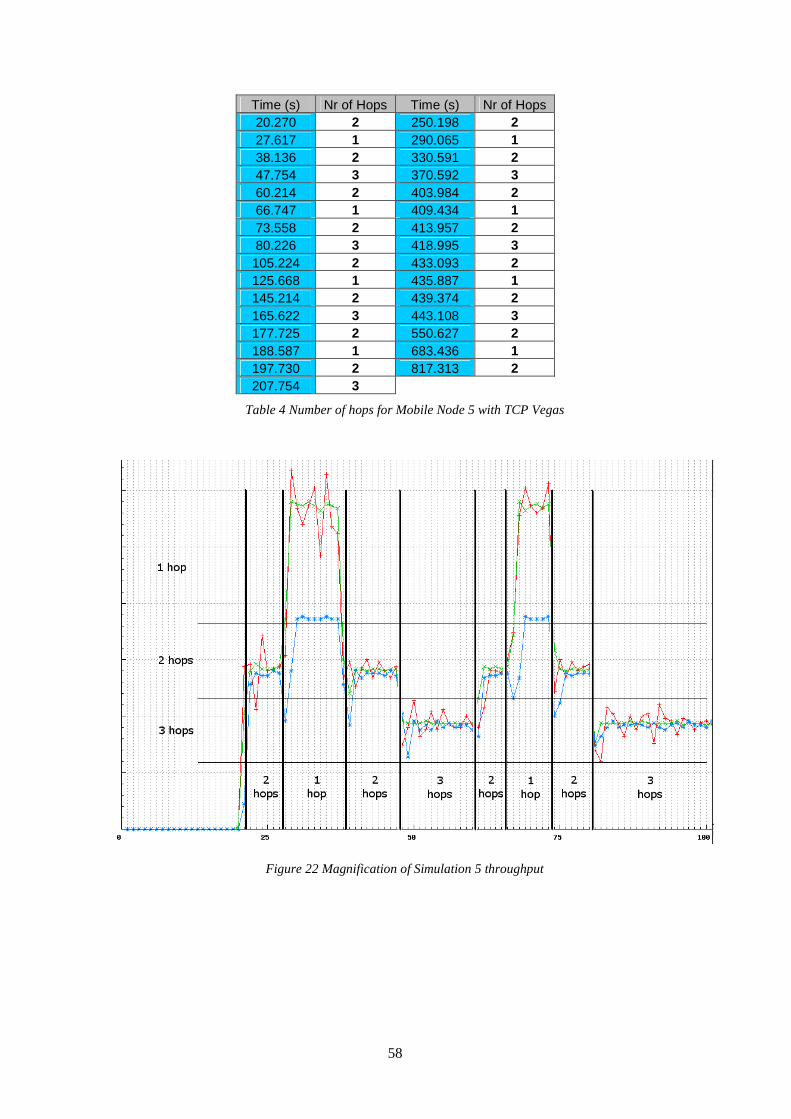
58
Time (s) Nr of Hops Time (s) Nr of Hops 20.270 2 250.198 2 27.617 1 290.065 1 38.136 2 330.591 2 47.754 3 370.592 3 60.214 2 403.984 2 66.747 1 409.434 1 73.558 2 413.957 2 80.226 3 418.995 3 105.224 2 433.093 2 125.668 1 435.887 1 145.214 2 439.374 2 165.622 3 443.108 3 177.725 2 550.627 2 188.587 1 683.436 1 197.730 2 817.313 2 207.754 3
Table 4 Number of hops for Mobile Node 5 with TCP Vegas
Figure 22 Magnification of Simulation 5 throughput
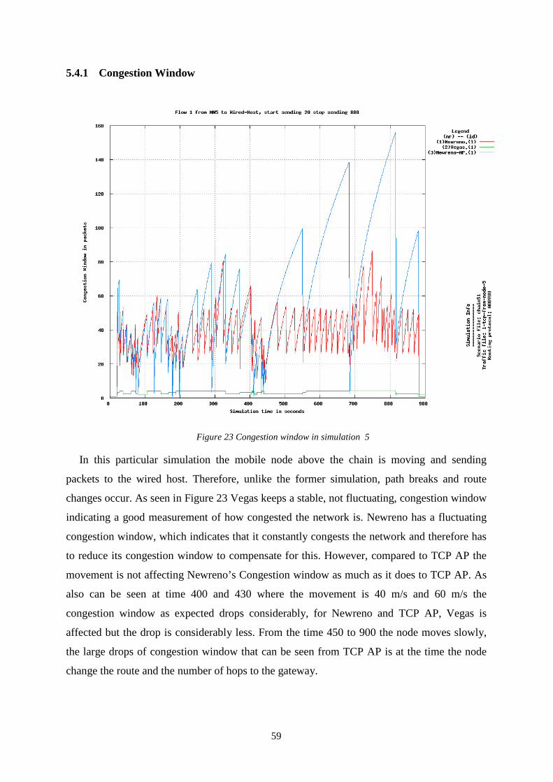
59
5.4.1 Congestion Window
Figure 23 Congestion window in simulation 5
In this particular simulation the mobile node above the chain is moving and sending
packets to the wired host. Therefore, unlike the former simulation, path breaks and route
changes occur. As seen in Figure 23 Vegas keeps a stable, not fluctuating, congestion window
indicating a good measurement of how congested the network is. Newreno has a fluctuating
congestion window, which indicates that it constantly congests the network and therefore has
to reduce its congestion window to compensate for this. However, compared to TCP AP the
movement is not affecting Newreno’s Congestion window as much as it does to TCP AP. As
also can be seen at time 400 and 430 where the movement is 40 m/s and 60 m/s the
congestion window as expected drops considerably, for Newreno and TCP AP, Vegas is
affected but the drop is considerably less. From the time 450 to 900 the node moves slowly,
the large drops of congestion window that can be seen from TCP AP is at the time the node
change the route and the number of hops to the gateway.
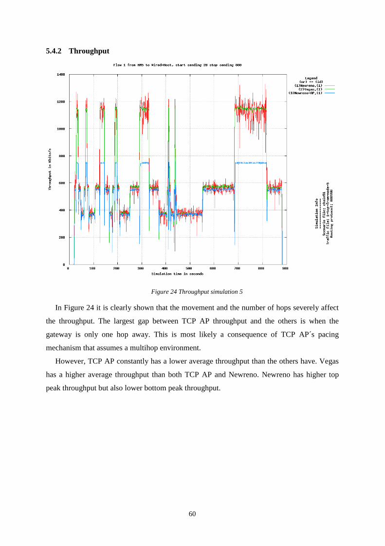
60
5.4.2 Throughput
Figure 24 Throughput simulation 5
In Figure 24 it is clearly shown that the movement and the number of hops severely affect
the throughput. The largest gap between TCP AP throughput and the others is when the
gateway is only one hop away. This is most likely a consequence of TCP AP´s pacing
mechanism that assumes a multihop environment.
However, TCP AP constantly has a lower average throughput than the others have. Vegas
has a higher average throughput than both TCP AP and Newreno. Newreno has higher top
peak throughput but also lower bottom peak throughput.
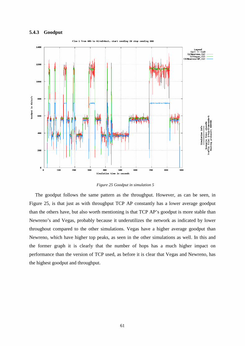
61
5.4.3 Goodput
Figure 25 Goodput in simulation 5
The goodput follows the same pattern as the throughput. However, as can be seen, in
Figure 25, is that just as with throughput TCP AP constantly has a lower average goodput
than the others have, but also worth mentioning is that TCP AP’s goodput is more stable than
Newreno’s and Vegas, probably because it underutilizes the network as indicated by lower
throughout compared to the other simulations. Vegas have a higher average goodput than
Newreno, which have higher top peaks, as seen in the other simulations as well. In this and
the former graph it is clearly that the number of hops has a much higher impact on
performance than the version of TCP used, as before it is clear that Vegas and Newreno, has
the highest goodput and throughput.
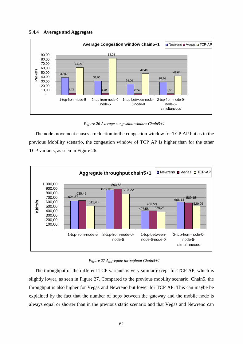
62
5.4.4 Average and Aggregate
Average congestion window chain5+1
39,09 31,06
24,00 28,74
3,19 2,24 2,59
61,90
83,08
47,49 42,64
3,43
- 10,00 20,00 30,00 40,00 50,00 60,00 70,00 80,00 90,00
1-tcp-from-node-5 2-tcp-from-node-0-node-5
1-tcp-between-node-5-node-0
2-tcp-from-node-0-node-5-
simultaneous
Pac
kets
Newreno Vegas TCP-AP
Figure 26 Average congestion window Chain5+1
The node movement causes a reduction in the congestion window for TCP AP but as in the
previous Mobility scenario, the congestion window of TCP AP is higher than for the other
TCP variants, as seen in Figure 26.
Aggregate throughput chain5+1
893,63
379,28
606,14
407,58
875,76
624,87 589,15
409,53
630,49
520,05
787,22
511,48
- 100,00 200,00 300,00 400,00 500,00 600,00 700,00 800,00 900,00
1.000,00
1-tcp-from-node-5 2-tcp-from-node-0-node-5
1-tcp-between-node-5-node-0
2-tcp-from-node-0-node-5-
simultaneous
Kbi
ts/s
Newreno Vegas TCP-AP
Figure 27 Aggregate throughput Chain5+1
The throughput of the different TCP variants is very similar except for TCP AP, which is
slightly lower, as seen in Figure 27. Compared to the previous mobility scenario, Chain5, the
throughput is also higher for Vegas and Newreno but lower for TCP AP. This can maybe be
explained by the fact that the number of hops between the gateway and the mobile node is
always equal or shorter than in the previous static scenario and that Vegas and Newreno can
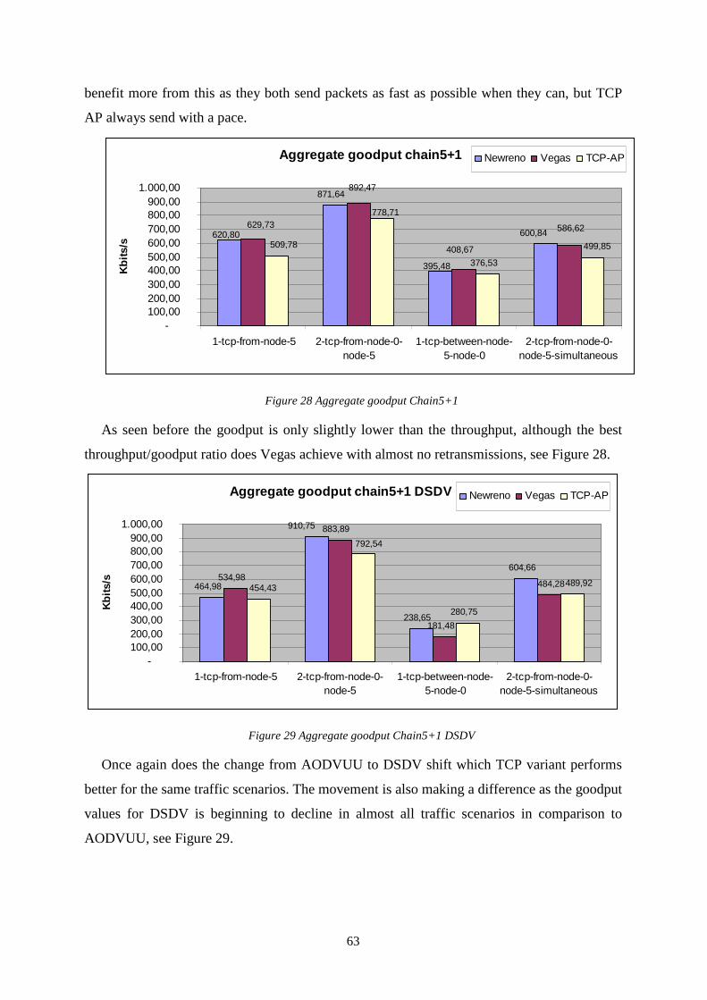
63
benefit more from this as they both send packets as fast as possible when they can, but TCP
AP always send with a pace.
Aggregate goodput chain5+1
376,53
600,84
395,48
871,64
620,80 586,62
408,67
892,47
629,73
499,85
778,71
509,78
- 100,00 200,00 300,00 400,00 500,00 600,00 700,00 800,00 900,00
1.000,00
1-tcp-from-node-5 2-tcp-from-node-0-node-5
1-tcp-between-node-5-node-0
2-tcp-from-node-0-node-5-simultaneous
Kbi
ts/s
Newreno Vegas TCP-AP
Figure 28 Aggregate goodput Chain5+1
As seen before the goodput is only slightly lower than the throughput, although the best
throughput/goodput ratio does Vegas achieve with almost no retransmissions, see Figure 28.
Aggregate goodput chain5+1 DSDV
464,98
238,65
604,66 534,98
883,89
181,48
280,75
910,75
484,28 489,92
792,54
454,43
- 100,00 200,00 300,00 400,00 500,00 600,00 700,00 800,00 900,00
1.000,00
1-tcp-from-node-5 2-tcp-from-node-0-node-5
1-tcp-between-node-5-node-0
2-tcp-from-node-0-node-5-simultaneous
Kbi
ts/s
Newreno Vegas TCP-AP
Figure 29 Aggregate goodput Chain5+1 DSDV
Once again does the change from AODVUU to DSDV shift which TCP variant performs
better for the same traffic scenarios. The movement is also making a difference as the goodput
values for DSDV is beginning to decline in almost all traffic scenarios in comparison to
AODVUU, see Figure 29.
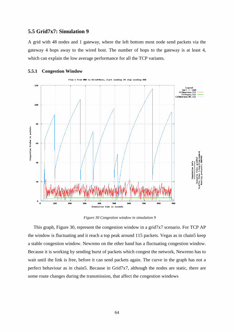
64
5.5 Grid7x7: Simulation 9
A grid with 48 nodes and 1 gateway, where the left bottom most node send packets via the
gateway 4 hops away to the wired host. The number of hops to the gateway is at least 4,
which can explain the low average performance for all the TCP variants.
5.5.1 Congestion Window
Figure 30 Congestion window in simulation 9
This graph, Figure 30, represent the congestion window in a grid7x7 scenario. For TCP AP
the window is fluctuating and it reach a top peak around 115 packets. Vegas as in chain5 keep
a stable congestion window. Newreno on the other hand has a fluctuating congestion window.
Because it is working by sending burst of packets which congest the network, Newreno has to
wait until the link is free, before it can send packets again. The curve in the graph has not a
perfect behaviour as in chain5. Because in Grid7x7, although the nodes are static, there are
some route changes during the transmission, that affect the congestion windows
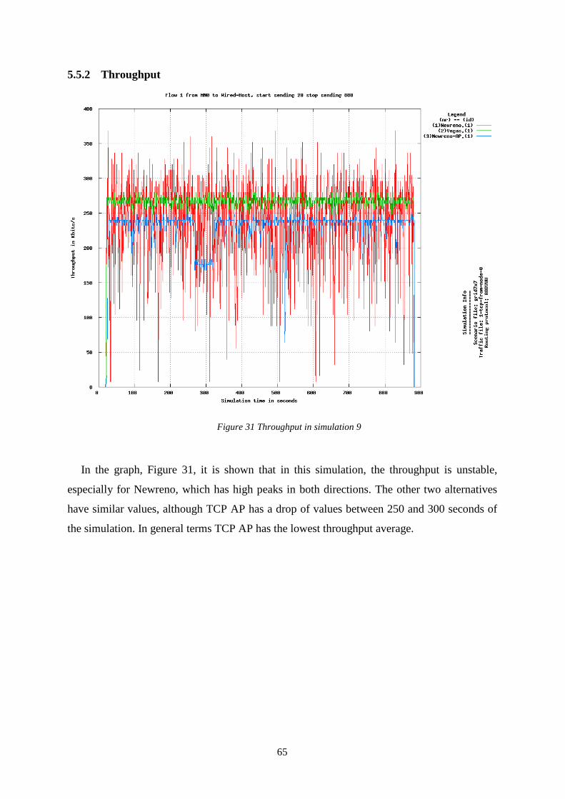
65
5.5.2 Throughput
Figure 31 Throughput in simulation 9
In the graph, Figure 31, it is shown that in this simulation, the throughput is unstable,
especially for Newreno, which has high peaks in both directions. The other two alternatives
have similar values, although TCP AP has a drop of values between 250 and 300 seconds of
the simulation. In general terms TCP AP has the lowest throughput average.
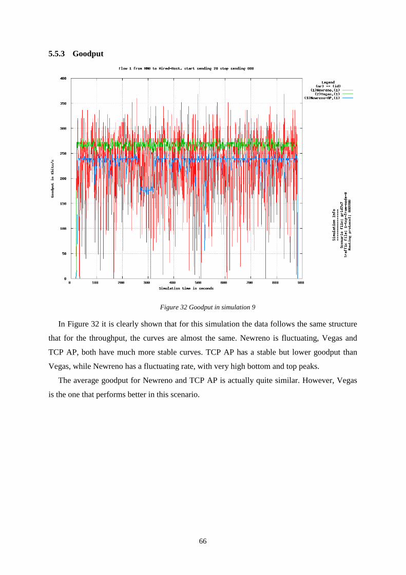
66
5.5.3 Goodput
Figure 32 Goodput in simulation 9
In Figure 32 it is clearly shown that for this simulation the data follows the same structure
that for the throughput, the curves are almost the same. Newreno is fluctuating, Vegas and
TCP AP, both have much more stable curves. TCP AP has a stable but lower goodput than
Vegas, while Newreno has a fluctuating rate, with very high bottom and top peaks.
The average goodput for Newreno and TCP AP is actually quite similar. However, Vegas
is the one that performs better in this scenario.
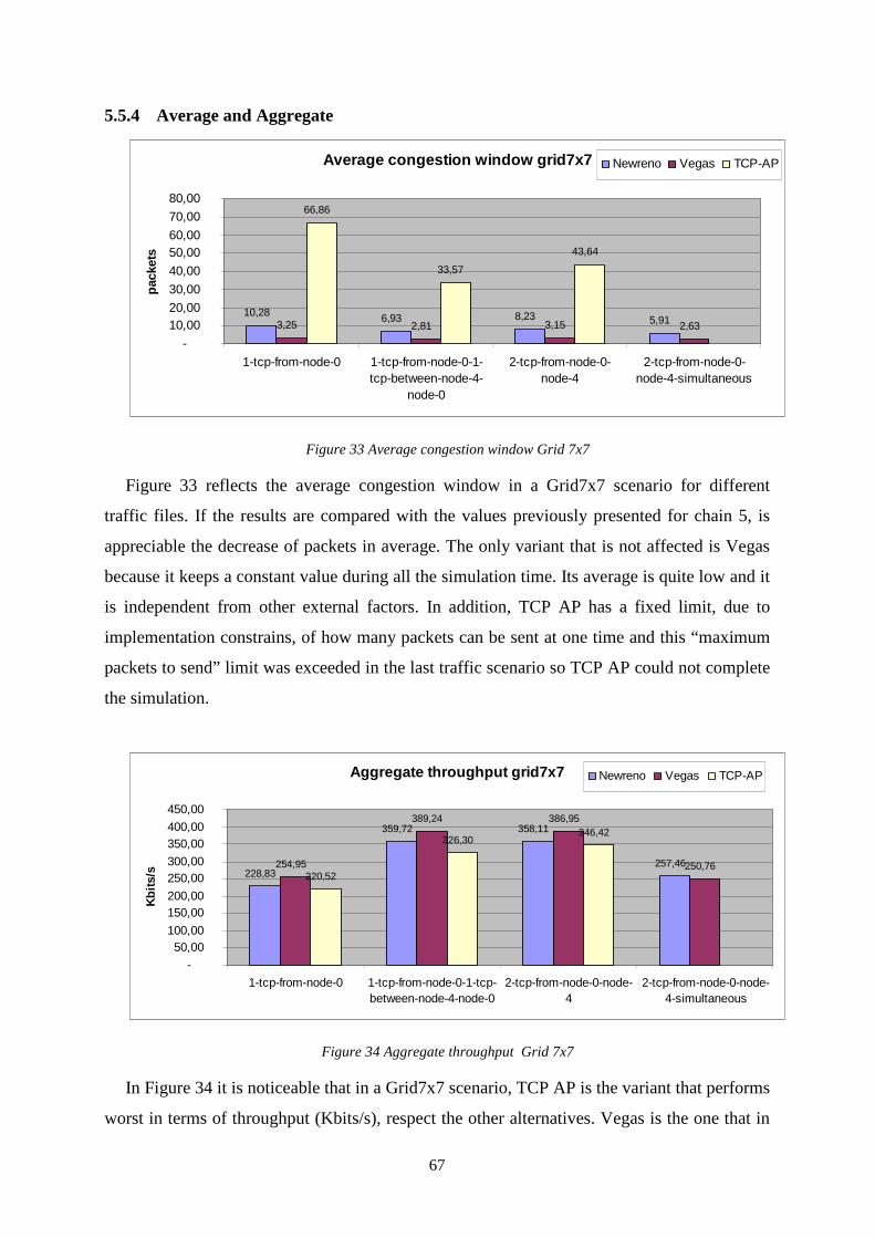
67
5.5.4 Average and Aggregate
Average congestion window grid7x7
10,28 6,93 8,23 5,91 3,25 2,81 3,15 2,63
66,86
33,57
43,64
-
10,00 20,00
30,00
40,00
50,00 60,00
70,00
80,00
1-tcp-from-node-0 1-tcp-from-node-0-1-tcp-between-node-4-
node-0
2-tcp-from-node-0-node-4
2-tcp-from-node-0-node-4-simultaneous
pack
ets
Newreno Vegas TCP-AP
Figure 33 Average congestion window Grid 7x7
Figure 33 reflects the average congestion window in a Grid7x7 scenario for different
traffic files. If the results are compared with the values previously presented for chain 5, is
appreciable the decrease of packets in average. The only variant that is not affected is Vegas
because it keeps a constant value during all the simulation time. Its average is quite low and it
is independent from other external factors. In addition, TCP AP has a fixed limit, due to
implementation constrains, of how many packets can be sent at one time and this “maximum
packets to send” limit was exceeded in the last traffic scenario so TCP AP could not complete
the simulation.
Aggregate throughput grid7x7
228,83
359,72 358,11
257,46 254,95
389,24 386,95
250,76 220,52
326,30 346,42
-
50,00 100,00
150,00 200,00
250,00 300,00
350,00 400,00
450,00
1-tcp-from-node-0 1-tcp-from-node-0-1-tcp-between-node-4-node-0
2-tcp-from-node-0-node-4
2-tcp-from-node-0-node-4-simultaneous
Kbi
ts/s
Newreno Vegas TCP-AP
Figure 34 Aggregate throughput Grid 7x7
In Figure 34 it is noticeable that in a Grid7x7 scenario, TCP AP is the variant that performs
worst in terms of throughput (Kbits/s), respect the other alternatives. Vegas is the one that in
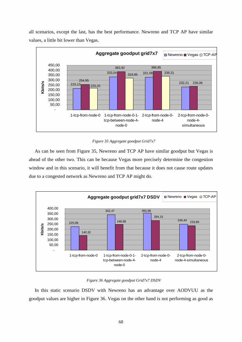
68
all scenarios, except the last, has the best performance. Newreno and TCP AP have similar
values, a little bit lower than Vegas.
Aggregate goodput grid7x7
215,13
333,04 331,08
232,21 254,95
383,92 386,85
236,06
339,31 319,95
220,32
- 50,00
100,00 150,00 200,00 250,00 300,00 350,00 400,00 450,00
1-tcp-from-node-0 1-tcp-from-node-0-1-tcp-between-node-4-
node-0
2-tcp-from-node-0-node-4
2-tcp-from-node-0-node-4-
simultaneous
Kbi
ts/s
Newreno Vegas TCP-AP
Figure 35 Aggregate goodput Grid7x7
As can be seen from Figure 35, Newreno and TCP AP have similar goodput but Vegas is
ahead of the other two. This can be because Vegas more precisely determine the congestion
window and in this scenario, it will benefit from that because it does not cause route updates
due to a congested network as Newreno and TCP AP might do.
Aggregate goodput grid7x7 DSDV
225,99
342,47
249,44
355,98
140,32
248,88
284,15
233,89
-
50,00 100,00
150,00
200,00
250,00 300,00
350,00
400,00
1-tcp-from-node-0 1-tcp-from-node-0-1-tcp-between-node-4-
node-0
2-tcp-from-node-0-node-4
2-tcp-from-node-0-node-4-simultaneous
Kbi
ts/s
Newreno Vegas TCP-AP
Figure 36 Aggregate goodput Grid7x7 DSDV
In this static scenario DSDV with Newreno has an advantage over AODVUU as the
goodput values are higher in Figure 36. Vegas on the other hand is not performing as good as
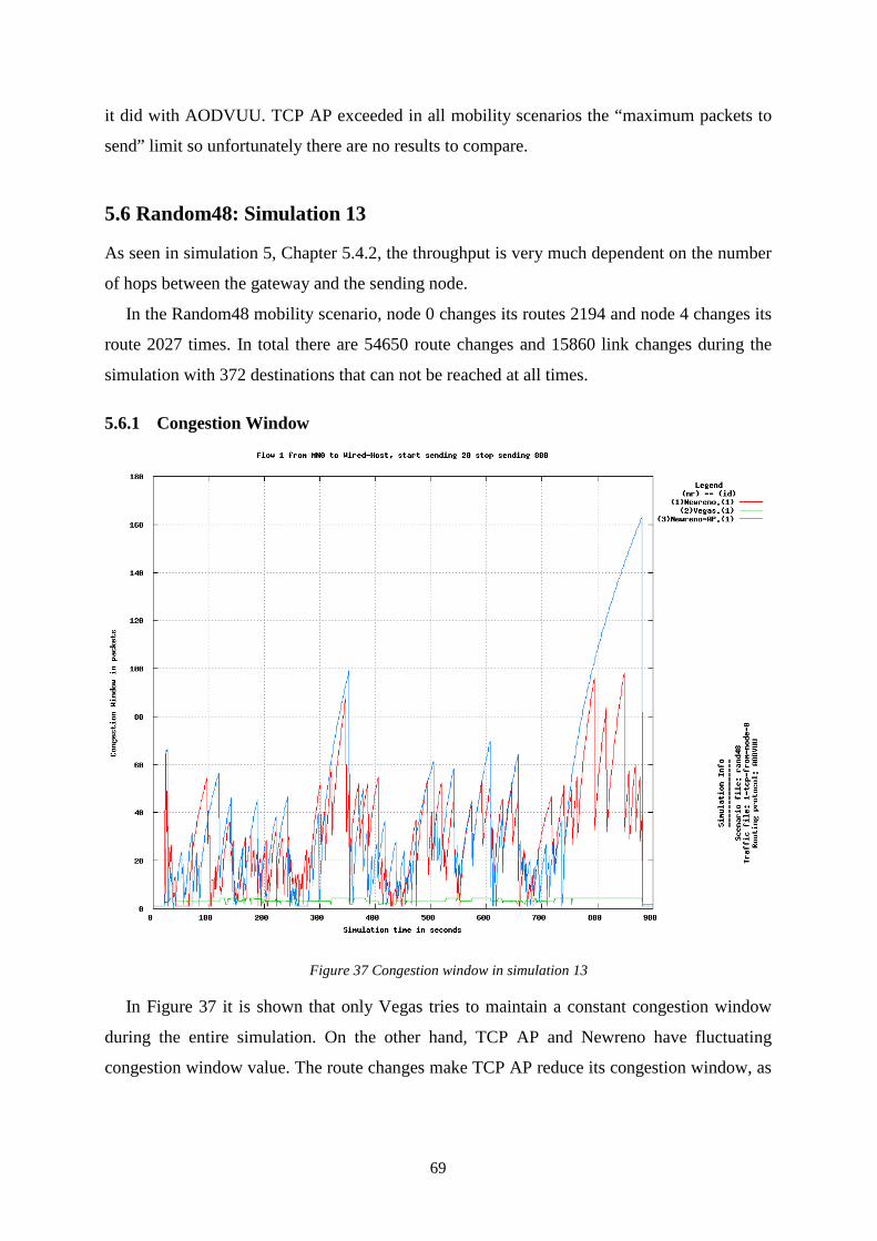
69
it did with AODVUU. TCP AP exceeded in all mobility scenarios the “maximum packets to
send” limit so unfortunately there are no results to compare.
5.6 Random48: Simulation 13
As seen in simulation 5, Chapter 5.4.2, the throughput is very much dependent on the number
of hops between the gateway and the sending node.
In the Random48 mobility scenario, node 0 changes its routes 2194 and node 4 changes its
route 2027 times. In total there are 54650 route changes and 15860 link changes during the
simulation with 372 destinations that can not be reached at all times.
5.6.1 Congestion Window
Figure 37 Congestion window in simulation 13
In Figure 37 it is shown that only Vegas tries to maintain a constant congestion window
during the entire simulation. On the other hand, TCP AP and Newreno have fluctuating
congestion window value. The route changes make TCP AP reduce its congestion window, as
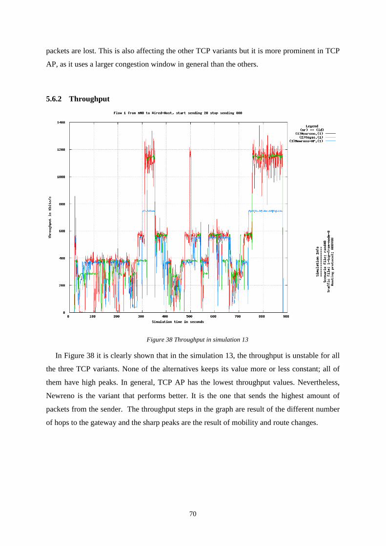
70
packets are lost. This is also affecting the other TCP variants but it is more prominent in TCP
AP, as it uses a larger congestion window in general than the others.
5.6.2 Throughput
Figure 38 Throughput in simulation 13
In Figure 38 it is clearly shown that in the simulation 13, the throughput is unstable for all
the three TCP variants. None of the alternatives keeps its value more or less constant; all of
them have high peaks. In general, TCP AP has the lowest throughput values. Nevertheless,
Newreno is the variant that performs better. It is the one that sends the highest amount of
packets from the sender. The throughput steps in the graph are result of the different number
of hops to the gateway and the sharp peaks are the result of mobility and route changes.
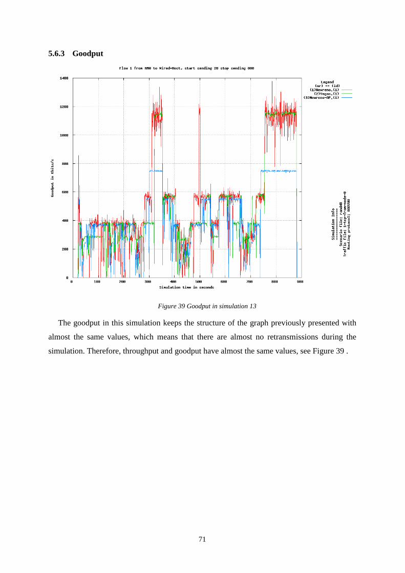
71
5.6.3 Goodput
Figure 39 Goodput in simulation 13
The goodput in this simulation keeps the structure of the graph previously presented with
almost the same values, which means that there are almost no retransmissions during the
simulation. Therefore, throughput and goodput have almost the same values, see Figure 39 .
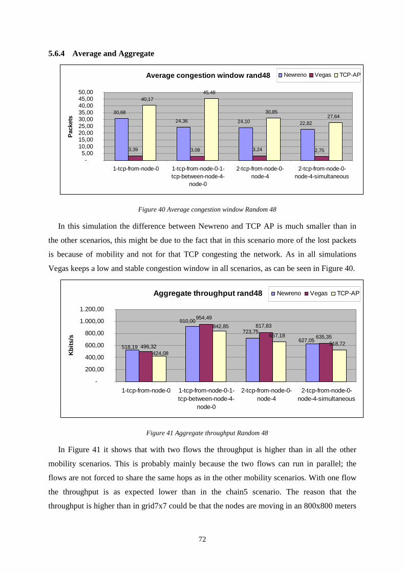
72
5.6.4 Average and Aggregate
Average congestion window rand48
30,68
24,36 24,10 22,82
3,39 3,08 3,24 2,75
40,17 45,48
30,85 27,64
- 5,00
10,00 15,00 20,00 25,00 30,00 35,00 40,00 45,00 50,00
1-tcp-from-node-0 1-tcp-from-node-0-1-tcp-between-node-4-
node-0
2-tcp-from-node-0-node-4
2-tcp-from-node-0-node-4-simultaneous
Pac
kets
Newreno Vegas TCP-AP
Figure 40 Average congestion window Random 48
In this simulation the difference between Newreno and TCP AP is much smaller than in
the other scenarios, this might be due to the fact that in this scenario more of the lost packets
is because of mobility and not for that TCP congesting the network. As in all simulations
Vegas keeps a low and stable congestion window in all scenarios, as can be seen in Figure 40.
Aggregate throughput rand48
723,75
954,49
817,83
635,35 657,18
518,72 627,05
910,00
518,19 496,32
842,85
424,08
-
200,00
400,00
600,00
800,00
1.000,00
1.200,00
1-tcp-from-node-0 1-tcp-from-node-0-1-tcp-between-node-4-
node-0
2-tcp-from-node-0-node-4
2-tcp-from-node-0-node-4-simultaneous
Kbi
ts/s
Newreno Vegas TCP-AP
Figure 41 Aggregate throughput Random 48
In Figure 41 it shows that with two flows the throughput is higher than in all the other
mobility scenarios. This is probably mainly because the two flows can run in parallel; the
flows are not forced to share the same hops as in the other mobility scenarios. With one flow
the throughput is as expected lower than in the chain5 scenario. The reason that the
throughput is higher than in grid7x7 could be that the nodes are moving in an 800x800 meters
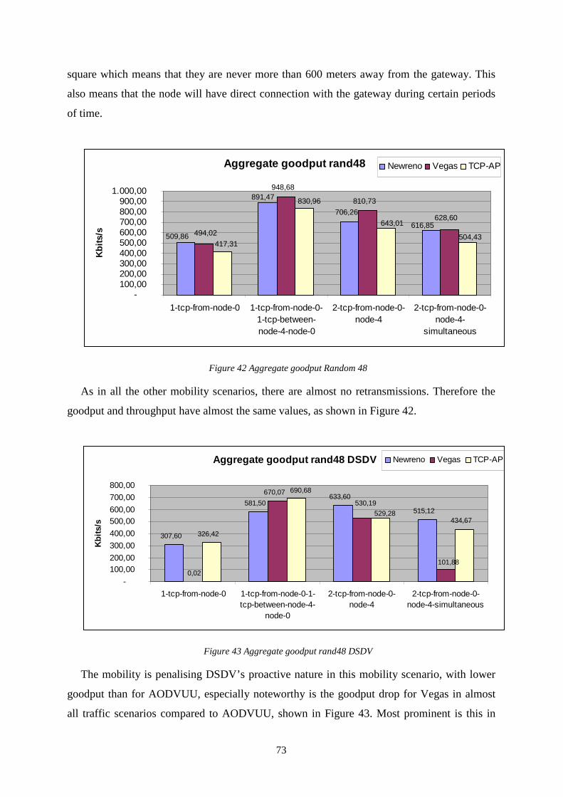
73
square which means that they are never more than 600 meters away from the gateway. This
also means that the node will have direct connection with the gateway during certain periods
of time.
Aggregate goodput rand48
706,26
948,68
810,73 891,47
616,85
509,86
628,60
494,02 504,43
643,01
830,96
417,31
- 100,00 200,00 300,00 400,00 500,00 600,00 700,00 800,00 900,00
1.000,00
1-tcp-from-node-0 1-tcp-from-node-0-1-tcp-between-node-4-node-0
2-tcp-from-node-0-node-4
2-tcp-from-node-0-node-4-
simultaneous
Kbi
ts/s
Newreno Vegas TCP-AP
Figure 42 Aggregate goodput Random 48
As in all the other mobility scenarios, there are almost no retransmissions. Therefore the
goodput and throughput have almost the same values, as shown in Figure 42.
Aggregate goodput rand48 DSDV
307,60
581,50 633,60
515,12
670,07
326,42
434,67
0,02
101,88
530,19
529,28
690,68
-
100,00 200,00
300,00
400,00
500,00 600,00
700,00
800,00
1-tcp-from-node-0 1-tcp-from-node-0-1-tcp-between-node-4-
node-0
2-tcp-from-node-0-node-4
2-tcp-from-node-0-node-4-simultaneous
Kbi
ts/s
Newreno Vegas TCP-AP
Figure 43 Aggregate goodput rand48 DSDV
The mobility is penalising DSDV’s proactive nature in this mobility scenario, with lower
goodput than for AODVUU, especially noteworthy is the goodput drop for Vegas in almost
all traffic scenarios compared to AODVUU, shown in Figure 43. Most prominent is this in
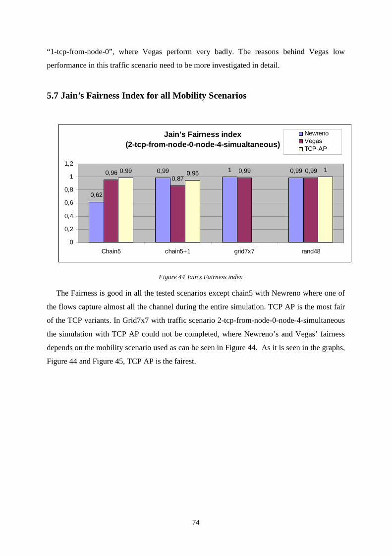
74
“1-tcp-from-node-0”, where Vegas perform very badly. The reasons behind Vegas low
performance in this traffic scenario need to be more investigated in detail.
5.7 Jain’s Fairness Index for all Mobility Scenarios
Jain's Fairness index (2-tcp-from-node-0-node-4-simualtaneous)
0,62
0,99 1 0,990,960,87
0,99 0,990,99 0,95 1
0
0,2
0,4
0,6
0,8
1
1,2
Chain5 chain5+1 grid7x7 rand48
NewrenoVegasTCP-AP
Figure 44 Jain's Fairness index
The Fairness is good in all the tested scenarios except chain5 with Newreno where one of
the flows capture almost all the channel during the entire simulation. TCP AP is the most fair
of the TCP variants. In Grid7x7 with traffic scenario 2-tcp-from-node-0-node-4-simultaneous
the simulation with TCP AP could not be completed, where Newreno’s and Vegas’ fairness
depends on the mobility scenario used as can be seen in Figure 44. As it is seen in the graphs,
Figure 44 and Figure 45, TCP AP is the fairest.
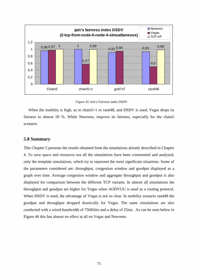
75
jain's fairness index DSDV(2-tcp-from-node-0-node-4-simualtaneous)
0,96 10,91 0,930,97
0,57
0,94
0,5
1 0,99 0,98
0
0,2
0,4
0,6
0,8
1
1,2
Chain5 chain5+1 grid7x7 rand48
NewrenoVegasTCP-AP
Figure 45 Jain's Fairness index DSDV
When the mobility is high, as in chain5+1 or rand48, and DSDV is used, Vegas drops its
fairness to almost 50 %. While Newreno, improve its fairness, especially for the chain5
scenario.
5.8 Summary
This Chapter 5 presents the results obtained from the simulations already described in Chapter
4. To save space and resources not all the simulations have been commented and analyzed,
only the template simulations, which try to represent the most significant situations. Some of
the parameters considered are: throughput, congestion window and goodput displayed as a
graph over time. Average congestion window and aggregate throughput and goodput is also
displayed for comparison between the different TCP variants. In almost all simulations the
throughput and goodput are higher for Vegas when AODVUU is used as a routing protocol.
When DSDV is used, the advantage of Vegas is not so clear. In mobility scenario rand48 the
goodput and throughput dropped drastically for Vegas. The same simulations are also
conducted with a wired-bandwidth of 756Kbits and a delay of 25ms. As can be seen below in
Figure 46 this has almost no effect at all on Vegas and Newreno.
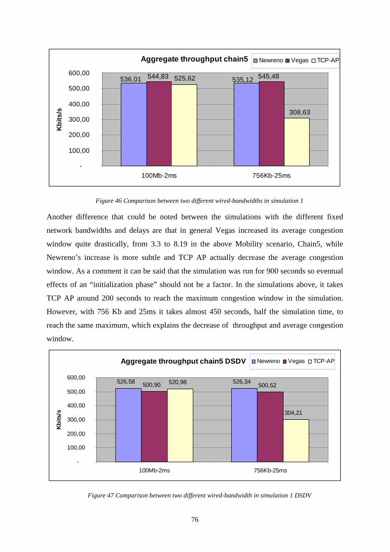
76
Aggregate throughput chain5
536,01 535,12 544,83 545,48 525,62
308,63
-
100,00
200,00
300,00
400,00
500,00
600,00
100Mb-2ms 756Kb-25ms
Kbi
ts/s
Newreno Vegas TCP-AP
Figure 46 Comparison between two different wired-bandwidths in simulation 1
Another difference that could be noted between the simulations with the different fixed
network bandwidths and delays are that in general Vegas increased its average congestion
window quite drastically, from 3.3 to 8.19 in the above Mobility scenario, Chain5, while
Newreno’s increase is more subtle and TCP AP actually decrease the average congestion
window. As a comment it can be said that the simulation was run for 900 seconds so eventual
effects of an “initialization phase” should not be a factor. In the simulations above, it takes
TCP AP around 200 seconds to reach the maximum congestion window in the simulation.
However, with 756 Kb and 25ms it takes almost 450 seconds, half the simulation time, to
reach the same maximum, which explains the decrease of throughput and average congestion
window.
Aggregate throughput chain5 DSDV
526,58 526,34 500,90 500,52 520,98
304,21
-
100,00
200,00
300,00
400,00
500,00
600,00
100Mb-2ms 756Kb-25ms
Kbi
ts/s
Newreno Vegas TCP-AP
Figure 47 Comparison between two different wired-bandwidth in simulation 1 DSDV
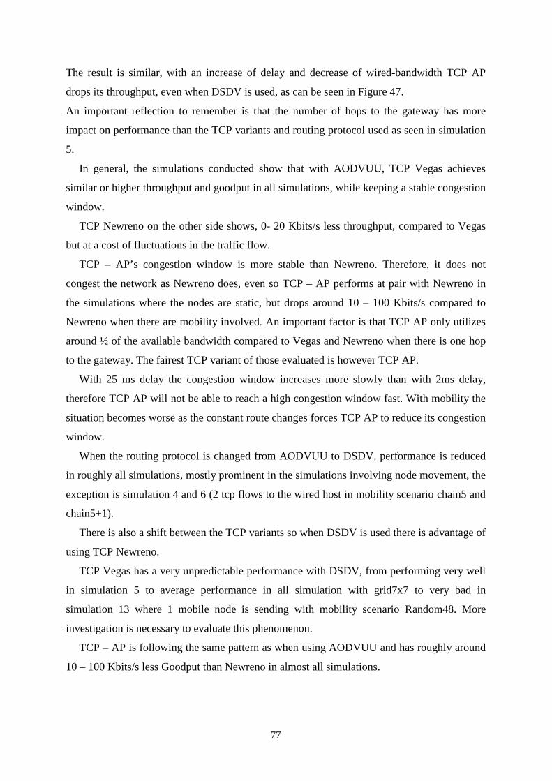
77
The result is similar, with an increase of delay and decrease of wired-bandwidth TCP AP
drops its throughput, even when DSDV is used, as can be seen in Figure 47.
An important reflection to remember is that the number of hops to the gateway has more
impact on performance than the TCP variants and routing protocol used as seen in simulation
5.
In general, the simulations conducted show that with AODVUU, TCP Vegas achieves
similar or higher throughput and goodput in all simulations, while keeping a stable congestion
window.
TCP Newreno on the other side shows, 0- 20 Kbits/s less throughput, compared to Vegas
but at a cost of fluctuations in the traffic flow.
TCP – AP’s congestion window is more stable than Newreno. Therefore, it does not
congest the network as Newreno does, even so TCP – AP performs at pair with Newreno in
the simulations where the nodes are static, but drops around 10 – 100 Kbits/s compared to
Newreno when there are mobility involved. An important factor is that TCP AP only utilizes
around ½ of the available bandwidth compared to Vegas and Newreno when there is one hop
to the gateway. The fairest TCP variant of those evaluated is however TCP AP.
With 25 ms delay the congestion window increases more slowly than with 2ms delay,
therefore TCP AP will not be able to reach a high congestion window fast. With mobility the
situation becomes worse as the constant route changes forces TCP AP to reduce its congestion
window.
When the routing protocol is changed from AODVUU to DSDV, performance is reduced
in roughly all simulations, mostly prominent in the simulations involving node movement, the
exception is simulation 4 and 6 (2 tcp flows to the wired host in mobility scenario chain5 and
chain5+1).
There is also a shift between the TCP variants so when DSDV is used there is advantage of
using TCP Newreno.
TCP Vegas has a very unpredictable performance with DSDV, from performing very well
in simulation 5 to average performance in all simulation with grid7x7 to very bad in
simulation 13 where 1 mobile node is sending with mobility scenario Random48. More
investigation is necessary to evaluate this phenomenon.
TCP – AP is following the same pattern as when using AODVUU and has roughly around
10 – 100 Kbits/s less Goodput than Newreno in almost all simulations.
78
6 Conclusions and Future Work
In this chapter some conclusions from the theoretical overview and an evaluation of the
results described in Chapter 5, will be presented with a suggestion of future work needed.
6.1 Conclusions
In this thesis we have looked in to several aspects of TCP performance in a hybrid
MANET, using a simulation based approach, where mobile nodes connect to a wired host
through a gateway.
The evaluation was conducted as a comparison between three TCP variants: TCP
Newreno, TCP Vegas and TCP AP, and two different routing protocols: AODVUU and
DSDV, which support gateway interconnection.
AODVUU is using the half-tunnelling approach and proxy RREP’s find and to route
packets to the wired network, while DSDV is using default route and next hop routing.
The evaluation of the simulations shows that AODVUU with TCP Vegas achieves at pair
or higher throughput and goodput in almost all simulations, while having the same or almost
the same fairness as TCP AP.
From the theoretical part, we conclude some details, although all these conclusions are not
based on the results obtained in our simulations.
MobileIP is very useful to be able to refer a node independently of the gateway or network
to which it is attached, the drawbacks is routing overhead and added complexity in the routing
protocol.
Half-tunnelling can be used in every network because no special requisite is required from
the network. Intermediate nodes in the transmission just forward the data as a normal packet
in the MANET; they do not have to constantly update their routing tables as needed with
default route; however the routing protocol must be changed at the sending node and gateway
to allow for handling of the extra routing header. Handovers are necessary to maintain the
communication with the network when nodes are forced to change gateway because of
mobility. Optimizing handovers could be very useful to reduce the amount of forced
handovers which are more costly, but it is important to choose the optimal point when it has
to be done, to not saturate the network with handovers. Several TCP variants have been
presented in Chapter 3, each one with different characteristics, as modified congestion
detection and pacing of the transmission. One interesting TCP variant, because of its ability to
79
not congest the network is TCP Few, which use a fractional window scheme to adapt better in
a network with a low BWD product, as a MANET.
As stated before, the focus on this thesis is to evaluate AODVUU and TCP AP, the other
TCP variants and routing protocol are used for comparison.
An important reflection to remember is that the number of hops to the gateway has more
impact on performance than the TCP variants.
In general, the simulations conducted show that with AODVUU, TCP Vegas achieves at
pair or higher Throughput and Goodput in all simulations, while keeping a stable congestion
window, which implies a good interpretation of the network congestion. The drawback of
having a low congestion window is of course the need to send a lot of ACK packets.
TCP Newreno on the other side performs almost as Vegas but at a cost of fluctuations in
the traffic flow. This congests the network and forces a reduction of the sending speed, which
is also reflected in the heavily fluctuating congestion window.
TCP AP performs at pair with Newreno in the simulations where the nodes are static, but
drops when there is mobility involved. An important factor is that TCP AP only utilizes
around ½ of the available bandwidth compared to Vegas and Newreno when there is one hop
to the gateway. The fairest TCP variant of those evaluated is however TCP AP.
With 25 ms delay the congestion window increases more slowly than with 2ms delay, this
is reflected in TCP AP as lower average throughput and goodput.
When the routing protocol is changed from AODVUU to DSDV, performance is reduced
in roughly all simulations.
There is also a shift between the TCP variants so when DSDV is used there is advantage of
using TCP Newreno as TCP Vegas has a very unpredictable performance with DSDV.
There are for sure more subtle interactions between the routing protocols and the TCP
variants that need to be further investigated. However, with the simulations conducted in this
thesis and the result thereof produced, our conclusion is therefore to use TCP Vegas in
combination with AODVUU for the fastest and most stable performance.
TCP AP for the fairest performance with a low amount of traffic burst.
In the simulations there is evidently so that the number of hops to the gateway have a great
impact on performance, and unfortunately TCP AP does not fully utilize this information.
80
6.2 Future work
An interesting extension of this work could be to test TCP-FeW performance with the same
simulations, mobility and traffic scenarios.
Another modification to the simulations would be to add more gateways and measure the
performance during handover. Traffic flows that come from the wired part could also be
interesting to evaluate.
Future tests could also be done to compare the results obtained against more generic
gateway discovery mechanisms as [16] and [37] to see how beneficial it is to integrate the
gateway discovery in the routing protocol as it is done with AODVUU and DSDV. This
would also allow for comparisons with other routing protocols like DSR or OLSR.
Modify TCP AP, so that it does not need to have a fixed value, or at least a larger value, of
the number of packets that can be on queue for sending. This would make TCP AP work in
more scenarios.
Another improvement for TCP AP would be to modify the protocol so it does not need
such large congestion window to fully utilize the bandwidth or alternatively make the
congestion window respond more quickly to changes in the network. Further enhancement to
TCP AP would be to make it actively take advantage of that the number of wireless hops is
one. ACK thinning, to reduce or delay the acks, could also be investigated as this has shown
to be beneficial for Vegas and Newreno [7]. Change the values of α and β, in Vegas, to
investigate the performance impact they have in a hybrid MANET environment.
A further investigation of how ELFN could benefit all TCP variants is also a viable way to
achieve improvement.
To further enlighten the results in this thesis, a more in depth investigation of the number of
hops, as when they occur and how they are affecting the performance, would be interesting.
Also interesting would be to investigate the interaction with more traffic flows and in a mixed
scenario with both UDP and TCP flows. Further investigation could also evaluate the routing
dependency in a more complex scenario with multiple gateways and multihop handovers.
7 References
[1] A. Aggrawal, S. Savage, T. Anderson. Understanding the Performance of TCP Pacing. INFOCOM 2000, Nineteenth Annual Joint Conference of the IEEE Computer and Communications Societies. IEEE, 2000. Volume: 3, pp. 1157-1165.
81
[2] G. Anastasi, A. Passarella. Towards a Novel Transport Protocol for Ad Hoc Networks. Proceedings of IFIP Int. Conference on Personal Wireless Communications (PWC 2003). Springer Verlag, 2003. pp. 23-25. 2003.
[3] J. Arkko, V. Devarapalli, F. Dupont. Using IPsec to Protect Mobile IPv6 Signaling Between Mobile Nodes and Home Agents, IETF RFC 3776. Jun 2004. [www] < http://www.ietf.org/rfc/rfc3776.txt?number=3776> (060515)
[4] L.S. Brakmo, L.L. Peterson. TCP Vegas: End to End Congestion Avoidance on a Global Internet. Journal on Selected Areas in Communications, IEEE,1999. Volume: 13, Issue: 8, pp. 1465-1480.
[5] J. Broch, D. A. Maltz, D. B. Johnson. Supporting hierarchy and heterogeneous interfaces in multi-hop wireless ad hoc networks. In Proceedings of the Workshop on Mobile Computing . IEEE, 1999.
[6] S.M. ElRakabawy, A. Klemm, C. Lindemann. TCP with Adaptive Pacing for Multihop Wireless Networks. Proceedings of the 6th ACM international symposium on Mobile ad hoc networking and computing. New York: ACM Press, 2005, pp. 288 – 299. 2005.
[7] S.M. ElRakabawy, C. Lindemann, M.K. Vernon. Improving TCP Performance for Multihop Wireless Networks. Proceedings of the 2005 International Conference on Dependable Systems and Networks (DSN'05), IEEE, 2005. Volume 00, pp. 684 – 693.
[8] K. Fall, K. Varadhan. The ns Manual (formerly ns Notes and Documentation. The VINT Project, Ch. 16.1.5: pp. 152, Ch. 16.2.1: pp 161, Jan 2005. [www] <http://www.isi.edu/nsnam/ns/doc/index.html> (060515), the chapter and page references is to the pdf version bundled with the ns2.28-allinone package [www] <http://www.isi.edu/nsnam/dist/ns-allinone-2.28.tar.gz> (060515)
[9] M. Ghassemian, V. Friderikos, H. Aghvami. Hybrid Handover in Multihop Radio Access Networks. Vehicular Technology Conference, 2005. VTC 2005-Spring. IEEE, 2005. Volume: 4, pp.2207- 2211
[10] M. Ghassemian, P. Hofmann, C. Prehofer, V. Friderikos, H. Aghvami. Performance Analysis of Internet Gateway Discovery Protocols in Ad Hoc Networks. Wireless Communications and Networking Conference, 2004. WCNC. 2004, IEEE, 2004. Volume: 1, pp. 120- 125.
[11] G. Hasegawa, M. Murata, H. Miyahara. Fairness and Stability of Congestion Control Mechanisms. Telecommunication Systems. Netherlands: Springer, 2000. Volume 15, Numbers 1-2, pp. 167 – 184.
[12] O. Ait Hellal, E. Altman. Analysis of TCP Vegas and TCP Reno. Telecommunication Systems. Netherlands: Springer, 2000. Volume 15, Numbers 3-4, pp. 381 – 404.
[13] P. Hofmann, C. Bettstetter, C. Prehofer. Performance Impact of Multihop Handovers in an IP-based Multihop Radio Access Network. ACM Mob Comp Comm Review, 2006.
[14] G. Holland, N. Vaidya. Analysis of TCP performance over mobile ad hoc networks. Wireless Networks. Netherlands: Springer, Mar 2002.Volume 8, Numbers 2-3, pp. 275 – 288.
[15] R. Jain, D. Chiu, W. Hawe, A Quantitative Measure of Fairness and Discrimination for Resource Allocation in Shared Systems, DEC Technical Report DEC-TR-301, Sep 1984.[www]<http://citeseer.ist.psu.edu>(060515)
82
[16] C. Jelger, T. Noel, A. Frey. Gateway and address autoconfiguration for IPv6 adhoc networks. IETF draft expired, draft-jelger-manet-gateway-autoconf-v6-02.txt, Apr 2004. [www] <http://www.watersprings.org/pub/id/draft-jelger-manet-gateway-autoconf-v6-02.txt> (060515)
[17] C. Jelger, T. Noel. Prefix Continuity and Global Address Autoconfiguration in IPv6 Ad Hoc Networks. Proceedings of the 4th Mediterranean Ad Hoc Networking Workshop (MedHocNet'05), Jun 2005.
[18] D. Johnson, C. Perkins, J. Arkko. Mobility Support in IPv6, IETF RFC 3775. Jun 2004. [www] <http://www.ietf.org/rfc/rfc3775.txt?number=3775> (060515)
[19] S. Low, L. Peterson, L. Wang. Understanding TCP Vegas: A Duality Model. Journal of the ACM. New York: ACM press, 2002. Volume 49, Issue 2, pp. 207 – 235.
[20] P. McCann. Mobile IPv6 Fast Handovers for 802.11 Networks. IETF RFC 4260. 2005 [www] <http://www.ietf.org/rfc/rfc4260.txt?number=4260> (060515)
[21] K. Nahm, A. Helmy, C.-C. Jay Kuo. TCP over 802.11 Multihop Networks: Issues and Performance Enhancement, presentation MobiHoc’05, 25-27 May 2005.
[22] K. Nahm, A. Helmy, C.-C. Jay Kuo. TCP over 802.11 Multihop Networks: Issues and Performance Enhancement, International Symposium on Mobile Ad Hoc Networking & Computing. New York: ACM press, 2005. pp. 277-287.
[23] T. Nandagopal T.E. Kim, X. Gao, V. Bharghavan, Achieving MAC Layer Fairness in Wireless Packet Networks. International Conference on Mobile Computing and Networking. New York: ACM press, 2000. pp. 87 - 98.
[24] A. Nilsson, AODV and IPv6 Internet Access for Ad hoc Networks. ACM SIGMOBILE Mobile Computing and Communication. New York: ACM press, 2002. Volume 6, Issue 3.
[25] A. Nilsson, A. Hamidian, U. Körner. Micro Mobility and Internet Access Performance for TCP connections in Ad hoc Networks. Proceedings of Nordic Teletraffic Seminar 17, Oslo, Norway, Aug 2004.
[26] E. Nordström, P. Gunningberg, C. Tschudin. Comparison of Gateway Forwarding Strategies in Ad hoc Networks. Technical Report 2004-007,Uppsala University. Mar 2004. [www] http://www.it.uu.se/research/reports/2004-007/2004-007-nc.pdf (060515)
[27] S, PalChaudhuri, S.Lavu. A Performance Comparison of Ad Hoc Network Routing Protocols. Rice University, 2000. [www] <http://citeseer.ist.psu.edu> (060515)
[28] C.E. Perkins, E. Belding-Royer, and S. Das. Ad hoc On Demand Distance Vector (AODV) Routing. IETF RFC 3561, Jul 2003. [www] <http://www.ietf.org/rfc/rfc3561.txt?number=3561> (060515)
[29] C.E. Perkins, P. Bhagwat, Highly Dynamic Destination- Sequenced Distance-Vector Routing (DSDV) for Mobile Computers, ACM SIGCOMM'94. London:University College, 1995. pp. 234-244.
[30] C.E. Perkins, J.T. Malinen, R. Wakikawa, E. Belding-Royer, Y. Sun, IP Address Autoconfiguration for Ad Hoc Networks, IETF draft expired, draft-perkins-manet-autoconf-01.txt, Nov 2001. [www] <http://www.watersprings.org/pub/id/draft-perkins-manet-autoconf-01.txt> (060515)
83
[31] C.E. Perkins, J.T. Malinen, R. Wakikawa, A. Nilsson, A.J. Tuominen. Internet connectivity for mobile ad hoc networks. Wireless Communications and Mobile Computing, Volume 2, Nr. 5,pp. 465-482. 2002
[32] C. Rohner, E. Nordström, P. Gunningberg, C. Tschudinn. Interactions between TCP, UDP and Routing Protocols in Wireless Multi-hop Ad hoc Networks. Proc. IEEE ICPS Workshop on Multi-hop Ad hoc Networks: from theory to reality (REALMAN’05), 2005.
[33] F.J. Ros, Pedro M. Ruiz and Antonio Gomez-Skarmeta. Performance Evaluation of Existing Approaches for Hybrid Ad Hoc Networks across Mobility Models. DIIC, University of Murcia, Jun 2005
[34] P.M. Ruiz, Antonio F. Gomez-Skarmeta. Enhanced Internet Connectivity for Hybrid Ad hoc Networks Through Adaptive Gateway Discovery. Local Computer Networks, 2004. 29th Annual IEEE International Conference on, Computer Society Press, 2004. pp-370-377.
[35] P.M. Ruiz, Francisco J. Ros, Antonio Gomez-Skarmeta. Internet Connectivity for Mobile Ad Hoc Networks: Solutions and Challenges. IEEE Communications Magazine, Oct 2005.
[36] C. Siva Ram Murthy and B. S. Manoj. Ad Hoc Wireless Networks, Architectures and Protocols, 3rd edition. Upper Saddle River, NJ:Prentice Hall, 2004.
[37] R. Wakikawa et al. Global connectivity for IPv6 Mobile Ad Hoc Networks. draft-wakikawa-manet-globalv6-05.txt, IETF draft, Mar 2006. [www] <http://www.ietf.org/internet-drafts/draft-wakikawa-manet-globalv6-05.txt> (060515)
[38] W. Chiung-Ying, L. Cheng-Ying, H. Ren-Hung, C Yuh-Shyan, Global Connectivity for Mobile IPv6-based Ad Hoc Networks, 19th International Conference on Advanced Information Networking and Applications (AINA'05), IEEE, 2005. Volume 2, pp. 807-812.
[39] X. Kaixin, B. Sang, L. Sungwook, M. Gerla. TCP Behavior across Multihop Wireless Networks and the Wired Internet. WoWMoM’02, New York:ACM press, 2002.
[40] The Uppsala University Ad Hoc Implementation Portal. [www] <http://core.it.uu.se/adhoc> (060516)
[41] UCB/LBNL/VINT. Network simulator - (version 2). 1999, [www] <http://www.isi.edu/nsnam/ns > (060516)
[42] CRIHAN, Centre de Ressources Informatiques de Haute-Normandie [www] <http://www.crihan.fr/res/syrhano/technique/ipv6> (060523)
[43] ISP Mobile Ad-Hoc Network Project, [www] <http://manet.isp.jp/image/AP_MANET2.gif > (060523)
[44] Internet Connectivity for MANET, presentation in Topics in Computer Networks [www] < http://www.cs.kau.se/cs/education/courses/davd08/p2/areas.php > (060523)
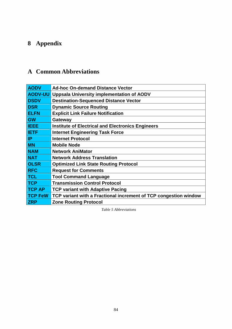
84
8 Appendix
A Common Abbreviations
AODV Ad-hoc On-demand Distance Vector AODV-UU Uppsala University implementation of AODV DSDV Destination-Sequenced Distance Vector DSR Dynamic Source Routing ELFN Explicit Link Failure Notification GW Gateway IEEE Institute of Electrical and Electronics Engine ers IETF Internet Engineering Task Force IP Internet Protocol MN Mobile Node NAM Network AniMator NAT Network Address Translation OLSR Optimized Link State Routing Protocol RFC Request for Comments TCL Tool Command Language TCP Transmission Control Protocol TCP AP TCP variant with Adaptive Pacing TCP FeW TCP variant with a Fractional increment of T CP congestion window ZRP Zone Routing Protocol
Table 5 Abbreviations
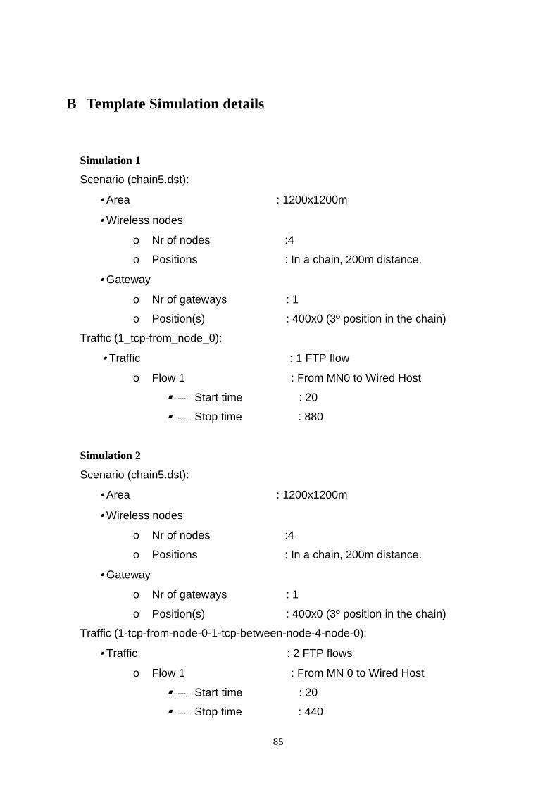
85
B Template Simulation details
Simulation 1
Scenario (chain5.dst):
• Area : 1200x1200m
• Wireless nodes
o Nr of nodes :4
o Positions : In a chain, 200m distance.
• Gateway
o Nr of gateways : 1
o Position(s) : 400x0 (3º position in the chain)
Traffic (1_tcp-from_node_0):
• Traffic : 1 FTP flow
o Flow 1 : From MN0 to Wired Host
��������� Start time : 20
��������� Stop time : 880
Simulation 2
Scenario (chain5.dst):
• Area : 1200x1200m
• Wireless nodes
o Nr of nodes :4
o Positions : In a chain, 200m distance.
• Gateway
o Nr of gateways : 1
o Position(s) : 400x0 (3º position in the chain)
Traffic (1-tcp-from-node-0-1-tcp-between-node-4-node-0):
• Traffic : 2 FTP flows
o Flow 1 : From MN 0 to Wired Host
��������� Start time : 20
��������� Stop time : 440
86
o Flow 2 : From MN4 to MN0
��������� Start time : 220
��������� Stop time : 880
Simulation 3
Scenario (chain5.dst):
• Area : 1200x1200m
• Wireless nodes
o Nr of nodes :4
o Positions : In a chain, 200m distance.
• Gateway
o Nr of gateways : 1
o Position(s) : 400x0 (3º position in the chain)
Traffic (2-tcp-from-node-0-node-4-simultaneous):
• Traffic : 2 FTP flows
o Flow 1 : From MN 0 to Wired Host
��������� Start time : 20
��������� Stop time : 880
o Flow 2 : From MN 4 to Wired Host
��������� Start time : 20
��������� Stop time : 880
Simulation 4
Scenario (chain5.dst):
• Area : 1200x1200m
• Wireless nodes
o Nr of nodes :4
o Positions : In a chain, 200m distance.
• Gateway
o Nr of gateways : 1
o Position(s) : 400x0 (3º position in the chain)
87
Traffic (2_tcp-from_node_0_node4):
• Traffic : 2 FTP flows
o Flow 1 : From MN 0 to Wired Host
��������� Start time : 20
��������� Stop time : 440
o Flow 2 : From MN 4 to Wired Host
��������� Start time : 220
��������� Stop time : 880
Simulation 5
Scenario (chain51.dst):
• Area : 1200x1200m
• Wireless nodes
o Nr of nodes :5
o Positions : chain, 200m distance. one 200 m above moving
• Gateway
o Nr of gateways : 1
o Position(s) : 400x0 (3º position in the chain)
Traffic (1_tcp-from_node_5):
• Traffic : 1 FTP flows
o Flow 1 : From MN5 to Wired Host.
��������� Start time : 20
��������� Stop time : 880
Simulation 6
Scenario (chain51.dst):
• Area : 1200x1200m
• Wireless nodes
o Nr of nodes :5
o Positions : chain, 200m distance. one 200 m above moving
• Gateway
o Nr of gateways : 1
88
o Position(s) : 400x0 (3º position in the chain)
Traffic (2-tcp-from-node-0-node-5):
• Traffic : 2 FTP flows
o Flow 1 : From MN0 to Wired Host.
��������� Start time : 20
��������� Stop time : 440
o Flow 2 : From MN5 to Wired Host.
��������� Start time : 220
��������� Stop time : 880
Simulation 7
Scenario (chain51.dst):
• Area : 1200x1200m
• Wireless nodes
o Nr of nodes :5
o Positions : chain, 200m distance. one 200 m above moving
• Gateway
o Nr of gateways : 1
o Position(s) : 400x0 (3º position in the chain)
Traffic (1_tcp-between_node_5-node_0):
• Traffic : 1 FTP flows
o Flow 1 : From MN5 to MN0.
��������� Start time : 20
��������� Stop time : 880
Simulation 8
Scenario (chain51.dst):
• Area : 1200x1200m
• Wireless nodes
o Nr of nodes :5
o Positions : chain, 200m distance. one 200 m above moving
• Gateway
o Nr of gateways : 1
o Position(s) : 400x0 (3º position in the chain)
89
Traffic (2-tcp-from-node-0-node-5-simultaneous):
• Traffic : 2 FTP flows
o Flow 1 : From MN0 to Wired Host
��������� Start time : 20
��������� Stop time : 880
o Flow 2 : From MN 5 to Wired Host
��������� Start time : 20
��������� Stop time : 880
Simulation 9
Scenario (grid7x7.dst):
• Area : 1200x1200m
• Wireless nodes
o Nr of nodes : 48
o Positions : Grid 7x7, 200m distance (X,Y)
• Gateway
o Nr of gateways : 1
o Position(s) : 400x400 (position 16 in grid)
Traffic (1_tcp-from_node_0):
• Traffic : 1 FTP flow
o Flow 1 : From MN0 to Wired Host
��������� Start time : 20
��������� Stop time : 880
Simulation 10
Scenario (grid7x7.dst):
• Area : 1200x1200m
• Wireless nodes
o Nr of nodes : 48
o Positions : Grid 7x7, 200m distance (X,Y)
• Gateway
o Nr of gateways : 1
o Position(s) : 400x400 (position 16 in grid)
90
Traffic (1-tcp-from-node-0-1-tcp-between-node-4-node-0):
• Traffic : 2 FTP flows
o Flow 1 : From MN 0 to Wired Host
��������� Start time : 20
��������� Stop time : 440
o Flow 2 : From MN4 to MN0
��������� Start time : 220
��������� Stop time : 880
Simulation 11
Scenario (grid7x7.dst):
• Area : 1200x1200m
• Wireless nodes
o Nr of nodes : 48
o Positions : Grid 7x7, 200m distance (X,Y)
• Gateway
o Nr of gateways : 1
o Position(s) : 400x400 (position 16 in grid)
Traffic (2-tcp-from-node-0-node-4-simultaneous):
• Traffic : 2 FTP flows
o Flow 1 : From MN 0 to Wired Host
��������� Start time : 20
��������� Stop time : 880
o Flow 2 : From MN 4 to Wired Host
��������� Start time : 20
��������� Stop time : 880
Simulation 12
Scenario (grid7x7.dst):
• Area : 1200x1200m
• Wireless nodes
91
o Nr of nodes : 48
o Positions : Grid 7x7, 200m distance (X,Y)
• Gateway
o Nr of gateways : 1
o Position(s) : 400x400 (position 16 in grid)
Traffic (2_tcp-from_node_0_node4):
• Traffic : 2 FTP flows
o Flow 1 : From MN 0 to Wired Host
��������� Start time : 20
��������� Stop time : 440
o Flow 2 : From MN 4 to Wired Host
��������� Start time : 220
��������� Stop time : 880
Simulation 13
Scenario (rand48.dst):
• Area : 1200x1200m
• Wireless nodes
o Nr of nodes : 48
o Positions : Grid 7x7, 200m distance (X,Y)
• Gateway
o Nr of gateways : 1
o Position(s) : 400x400 (position 16 in grid)
Traffic (1_tcp-from_node_0):
• Traffic : 1 FTP flow
o Flow 1 : From MN0 to Wired Host
��������� Start time : 20
��������� Stop time : 880
Simulation 14
Scenario (rand48.dst):
• Area : 1200x1200m
• Wireless nodes
92
o Nr of nodes : 48
o Positions : Random in a 800x800 area (X,Y)
• Gateway
o Nr of gateways : 1
o Position(s) : 400x400
Traffic (1-tcp-from-node-0-1-tcp-between-node-4-node-0):
• Traffic : 2 FTP flows
o Flow 1 : From MN 0 to Wired Host
��������� Start time : 20
��������� Stop time : 440
o Flow 2 : From MN4 to MN0
��������� Start time : 220
��������� Stop time : 880
Simulation 15
Scenario (rand48.dst):
• Area : 1200x1200m
• Wireless nodes
o Nr of nodes : 48
o Positions : Random in a 800x800 area (X,Y)
• Gateway
o Nr of gateways : 1
o Position(s) : 400x400
Traffic (2-tcp-from-node-0-node-4-simultaneous):
• Traffic : 2 FTP flows
o Flow 1 : From MN 0 to Wired Host
��������� Start time : 20
��������� Stop time : 880
o Flow 2 : From MN 4 to Wired Host
��������� Start time : 20
��������� Stop time : 880
93
Simulation 16
Scenario (rand48.dst):
• Area : 1200x1200m
• Wireless nodes
o Nr of nodes : 48
o Positions : Random in a 800x800 area (X,Y)
• Gateway
o Nr of gateways : 1
o Position(s) : 400x400
Traffic (2_tcp-from_node_0_node4):
• Traffic : 2 FTP flows
o Flow 1 : From MN 0 to Wired Host
��������� Start time : 20
��������� Stop time : 440
o Flow 2 : From MN 4 to Wired Host
��������� Start time : 220
��������� Stop time : 880
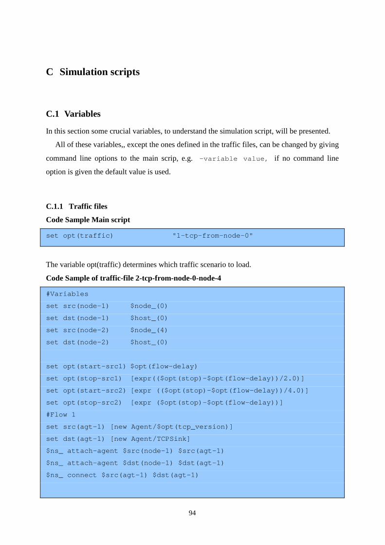
94
C Simulation scripts
C.1 Variables
In this section some crucial variables, to understand the simulation script, will be presented.
All of these variables,, except the ones defined in the traffic files, can be changed by giving
command line options to the main scrip, e.g. –variable value, if no command line
option is given the default value is used.
C.1.1 Traffic files
Code Sample Main script
set opt(traffic) "1-tcp-from-node-0"
The variable opt(traffic) determines which traffic scenario to load.
Code Sample of traffic-file 2-tcp-from-node-0-node-4
#Variables
set src(node-1) $node_(0)
set dst(node-1) $host_(0)
set src(node-2) $node_(4)
set dst(node-2) $host_(0)
set opt(start-src1) $opt(flow-delay)
set opt(stop-src1) [expr(($opt(stop)-$opt(flow-del ay))/2.0)]
set opt(start-src2) [expr (($opt(stop)-$opt(flow-de lay))/4.0)]
set opt(stop-src2) [expr ($opt(stop)-$opt(flow-del ay))]
#Flow 1
set src(agt-1) [new Agent/$opt(tcp_version)]
set dst(agt-1) [new Agent/TCPSink]
$ns_ attach-agent $src(node-1) $src(agt-1)
$ns_ attach-agent $dst(node-1) $dst(agt-1)
$ns_ connect $src(agt-1) $dst(agt-1)
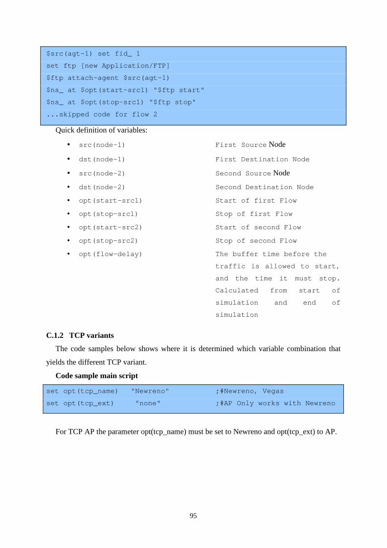
95
$src(agt-1) set fid_ 1
set ftp [new Application/FTP]
$ftp attach-agent $src(agt-1)
$ns_ at $opt(start-src1) "$ftp start"
$ns_ at $opt(stop-src1) "$ftp stop"
...skipped code for flow 2
Quick definition of variables:
• src(node-1) First Source Node
• dst(node-1) First Destination Node
• src(node-2) Second Source Node
• dst(node-2) Second Destination Node
• opt(start-src1) Start of first Flow
• opt(stop-src1) Stop of first Flow
• opt(start-src2) Start of second Flow
• opt(stop-src2) Stop of second Flow
• opt(flow-delay) The buffer time before the
traffic is allowed to start,
and the time it must stop.
Calculated from start of
simulation and end of
simulation
C.1.2 TCP variants
The code samples below shows where it is determined which variable combination that
yields the different TCP variant.
Code sample main script
set opt(tcp_name) "Newreno" ;#Newreno, Vegas
set opt(tcp_ext) "none" ;#AP Only works with Newr eno
For TCP AP the parameter opt(tcp_name) must be set to Newreno and opt(tcp_ext) to AP.
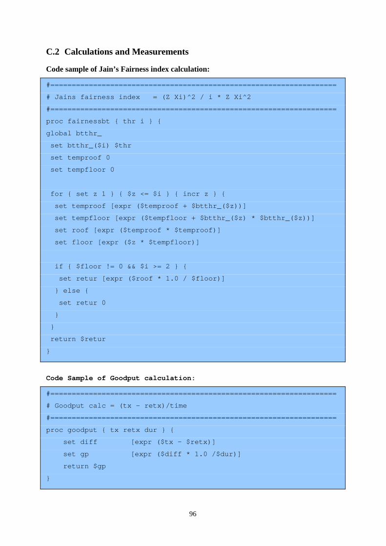
96
C.2 Calculations and Measurements
Code sample of Jain’s Fairness index calculation:
#================================================== =================
# Jains fairness index = (Z Xi)^2 / i * Z Xi^2
#================================================== =================
proc fairnessbt { thr i } {
global btthr_
set btthr_($i) $thr
set temproof 0
set tempfloor 0
for { set z 1 } { $z <= $i } { incr z } {
set temproof [expr ($temproof + $btthr_($z))]
set tempfloor [expr ($tempfloor + $btthr_($z) * $ btthr_($z))]
set roof [expr ($temproof * $temproof)]
set floor [expr ($z * $tempfloor)]
if { $floor != 0 && $i >= 2 } {
set retur [expr ($roof * 1.0 / $floor)]
} else {
set retur 0
}
}
return $retur
}
Code Sample of Goodput calculation:
#================================================== =================
# Goodput calc = (tx - retx)/time
#================================================== =================
proc goodput { tx retx dur } {
set diff [expr ($tx - $retx)]
set gp [expr ($diff * 1.0 /$dur)]
return $gp
}
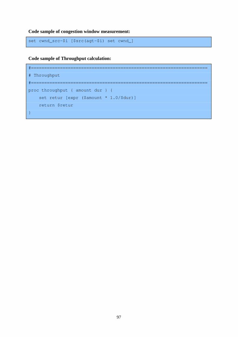
97
Code sample of congestion window measurement:
set cwnd_src-$i [$src(agt-$i) set cwnd_]
Code sample of Throughput calculation:
#================================================== =================
# Throughput
#================================================== =================
proc throughput { amount dur } {
set retur [expr ($amount * 1.0/$dur)]
return $retur
}
98
D Code
D.1 Main script
This script is the actual simulations script that controls the entire simulation.
# ================================================= ===================== # Define options # ================================================= ===================== #TCP version and upper bound on congestion window set opt(tcp_name) "Newreno" ;#FeW Newreno, Reno, T ahoe set opt(tcp_ext) "" ;#AP Only works with Newreno set opt(max_cwnd) 199 ;# < 200 for TCP AP set opt(max_win) 64 ;# < 200 for TCP AP
#Scenario files set opt(scenario) "chain5" set opt(traffic) "1-tcp-from-node-0" #set opt(traffic) "tcp" ;#"tcp","udp","mobiletcp" or traffic file set opt(src-node) 4 ;#Only used if no traffic file. src-node must exist ;#Destination is wired host or mobile node_(0) (if mobiletcp) ## Various parameters #Wireless set opt(rp) AODVUU ;# DSDV, AODVUUset opt(Wireless-rate) 2e6 #Wired set opt(Wired-Bandwidth) 100Mb set opt(Wired-Delay) 2ms #Start and stop parameters set opt(stop) 900.0 set opt(start-trace) 1.0 set opt(flow-delay) 20 #Clock in tracfiles set opt(granularity) 1.0
##Static Variables #Dirs set opt(result-dir) "./result" set opt(traffic-dir) "./traffic" set opt(scenario-dir) "./scenario"
##Wireless Network Interface Characteristics set opt(chan) Channel/WirelessChannel ;# channel type set opt(prop) Propagation/TwoRayGround ;# radio-propagation model set opt(netif) Phy/WirelessPhy ;# network interface type set opt(mac) Mac/802_11 ;# MAC type set opt(ifq) Queue/DropTail/PriQueue ;# interface queue type set opt(ll) LL ;# link layer type set opt(ant) Antenna/OmniAntenna ;# antenna model
99
set opt(ifqlen) 50 ;# max packet in ifq
#Set up the topography set opt(x) 1200 set opt(y) 1200
#Graph drawing variables set opt(same-x-axis) 1 set opt(xlabel) "Simulation time in seconds" set opt(yformat) "%g" set opt(xformat) "%g" set opt(ylabel-win) "Congestion Window in packets" set opt(ylabel-bt) "Throughput in Kbits/s" set opt(ylabel-btgp) "Goodput in Kbits/s" set opt(ylabel-pkt) "Throughput in pkts/s" set opt(ylabel-pktgp) "Throughput in pkts/s" set opt(ylabel-fair) "Jain's Fairness Index procen t" set opt(afterburner) -1
# ================================================= ===================== # Main # ================================================= ===================== proc main {} { global opt ns_ file_ argc argv #----Define some colors in NAM--------# set ns_ [new Simulator] $ns_ color 0 Brown $ns_ color 1 Blue $ns_ color 2 Yellow $ns_ color 3 Green $ns_ color 4 Purple $ns_ color 5 Red
#Load command line options getopt $argc $argv #$ns_ use-newtrace
#Initialize variables that might have changed via c md line initvar
#Create dirs set val(result_dir) "$opt(result-dir)/$opt(scenario)/$opt(traffic)/$opt(rp)-$opt(tcp _name)" exec mkdir -p "$val(result_dir)"
#----Remove old tracefile and open new one--------- -# set tracefile "$val(result_dir)/trace" exec rm -f "$tracefile.*"
#For NS set file_(tr) [open "$tracefile.tr" w] $ns_ trace-all $file_(tr)
#For NAM set file_(nam) [open "$tracefile.nam" w] #$ns_ namtrace-all-wireless $file_(nam) $opt(x) $op t(y)
#For Cwnd trace set file_(win) [open "$tracefile.win" w]
100
#For Bytes trace set file_(bt) [open "$tracefile.bt" w]
#For Packet trace set file_(pkt) [open "$tracefile.pkt" w]
#For Movment trace plotMovement ;#Write output in ns tracefile
#----Call the procedure that create topology, setup the traffic etc.---# create-topo-nodes set-traffic
#----------------------- Run Simulation ----------- -------------- $ns_ at $opt(stop).0001 "finish $tracefile $val(res ult_dir)" $ns_ at 0.0 "$ns_ set-animation-rate 15ms" #Starting the logging $ns_ at $opt(start-trace) "plotPktByteWin $file_(pk t) $file_(bt) $file_(win) 0.0" # For tracegraph puts $file_(tr) "mixed12 ip hex"
puts "Starting simulation..." puts "Please wait..." $ns_ run
}
# ================================================= ===================== # End of Simulation # ================================================= ===================== proc finish { tracefile result_dir } { global ns_ opt node_ host_ file_ dst src val #Statistics about simulation statPktByteWin $file_(pkt) $file_(bt) $file_(wi n) #--For NAM ----# #The Wired Host $ns_ at $opt(stop).01 "$host_(0) reset"; #The Wireless nodes + Gateway (remeber node_(X) = gw1) for {set i 0} {$i < [expr $opt(wirelessNodes) + $opt(gatewayNodes)]} {incr i} { $ns_ at $opt(stop).01 "$node_($i) reset"; } #Stop Animation $ns_ at $opt(stop).01 "$ns_ nam-end-wireless $o pt(stop)" #------Stop simulation------# $ns_ at $opt(stop).0002 "$ns_ halt" #Flush and close tracefiles $ns_ flush-trace flush $file_(tr) flush $file_(nam) flush $file_(win) flush $file_(bt) flush $file_(pkt)
101
close $file_(tr) close $file_(nam) close $file_(win) close $file_(bt) close $file_(pkt) #-----------Run NAM -------------# #puts "Running nam with $tracefile.nam ... " #exec nam "$tracefile.nam" & #-----------Post processin -------------# set post_dir "$result_dir/postprocess" exec mkdir -p "$post_dir" exec rm -f "$post_dir/*" puts "Running post-processing scripts ... " postProcessing $tracefile $post_dir $result_dir #writing the dir in afterburner file if { $opt(afterburner) != -1 } { set ab [open "$opt(afterburner)" a] puts $ab "$result_dir/$opt(afterburner)" flush $ab close $ab } #------------End post processing -----------# exit 0 } # ================================================= ===================== # Setup Scenario and Nodes # ================================================= ===================== proc create-topo-nodes {} { global ns_ opt node_ gw_ host_ god_ #create a topology object and define topology set topo [new Topography] $topo load_flatgrid $opt(x) $opt(y) create-nodes $topo #In scenario rand48 this is the gateways positi on if { $opt(scenario) == "rand48" } { $gw_(0) set X_ $opt(gw-pos-X) $gw_(0) set Y_ $opt(gw-pos-Y) $gw_(0) set Z_ $opt(gw-pos-Z) } #Load Scenario file if { $opt(scenario) == "" } { puts "*** NOTE: no scenario file specified. " set opt(scenario) "none" } else { puts "Loading scenario file..." source "$opt(scenario-dir)/$opt(scenario).d st" puts "Load complete..." } #---Label Mobile and Fixed hosts in NAM-------- -------" $ns_ at 0.0 "$host_(0) label \"Wired Host([$hos t_(0) id])\""
102
puts "Wired Host = Node_ID([$host_(0) id])" $ns_ at 0.0 "$gw_(0) label \"GATEWAY([$gw_(0) i d])\"" puts "GATEWAY = Node_ID([$gw_(0) id])" for {set i 0} {$i < [expr $opt(wirelessNodes) + $opt(gatewayNodes)] } {incr i} { if { $i != $opt(gwNode) } { $ns_ at 0.0 "$node_($i) label \"MN $i ( [$node_($i) id])\"" puts "MN $i = Node_ID([$node_($i) id])" $ns_ initial_node_pos $node_($i) 20 } }
$host_(0) color blue $host_(0) shape box $gw_(0) color red $gw_(0) shape hexagon #----- For Nam Wired Links----------# $ns_ duplex-link-op $host_(0) $gw_(0) orient up}
# ================================================= ===================== # Create nodes # ================================================= ===================== proc create-nodes { topo } { global ns_ opt node_ gw_ host_ god_ #------------Create God Object-------------# set god_ [create-god [expr $opt(wirelessNodes)+ $opt(gatewayNodes)]] #---------Addressing---------# #For mixed simulations we need to use hierarchi cal routing in order to #route packets. Must be put before addressing s tarts. $ns_ node-config -addressType hierarchical #Number of domains #2 domains AddrParams set domain_num_ 2 #Number of clusters in each domain #2 clusters #1 cluster in domain 0 #1 cluster in domain 1 AddrParams set cluster_num_ {1 1} #Number of nodes in each cluster #1 nodes in domain 0 in cluster 0: host1 0.0.0 #Wireless + gateway node in domain 1 in cluster 0 lappend nr_of_nodes_in_each_domain 1 [expr $opt(wirelessNodes)+$opt(gatewayNodes)] AddrParams set nodes_num_ $nr_of_nodes_in_each _domain #-----Create Nodes--------------------# ### Create wired nodes set host_(0) [$ns_ node 0.0.0]
# Configure mobile nodes and gateways $ns_ node-config -adhocRouting $opt(rp) \ -llType $opt(ll) \
103
-macType $opt(mac) \ -ifqType $opt(ifq) \ -ifqLen $opt(ifqlen) \ -antType $opt(ant) \ -propType $opt(prop) \ -phyType $opt(netif) \ -channel [new $opt(chan)] \ -topoInstance $topo \ -wiredRouting ON \ -agentTrace ON \ -routerTrace OFF \ -macTrace OFF \ -movementTrace OFF #Set wireless sending rate $opt(mac) set basicRate_ $opt(Wireless-rate) $opt(mac) set dataRate_ $opt(Wireless-rate) $opt(netif) set bandwidth_ $opt(Wireless-rate) $opt(netif) set Rb_ $opt(Wireless-rate) ### Create gateway set gw_(0) [$ns_ node 1.0.$opt(gwNode)] $gw_(0) random-motion 0 ;# disable random motio n #----- Create Wired Links----------# $ns_ duplex-link $host_(0) $gw_(0) $opt(Wired-B andwidth) $opt(Wired-Delay) DropTail #set ragent [$ns_ create-noah-agent $gw1] #If AODVUU is used tell this node that it is a gateway and use half tunneling if { $opt(rp) == "AODVUU" } { set r [$gw_(0) set ragent_] $r set internet_gw_mode_ 1 } #In all scenarios except rand48 the gateway's p osition ##is defined in the sceanrio file as node_(X) set node_($opt(gwNode)) $gw_(0) # Configure for mobile nodes $ns_ node-config -wiredRouting OFF ### Create mobile nodes for {set i 0} {$i < [expr $opt(wirelessNodes) + $opt(gatewayNodes)] } {incr i} { if { $i != $opt(gwNode) } { ;#Gateway node is already created set node_($i) [$ns_ node 1.0.$i] $node_($i) random-motion 0 $node_($i) base-station [AddrParams add r2id [$gw_(0) node-addr]] ;# assign gw_(0) as gateway for this node } } }
# ================================================= ===================== # Setup Traffic # ================================================= =====================
104
proc set-traffic { } { global ns_ opt node_ gw_ host_ src dst if { $opt(max_cwnd) != -1 } { Agent/$opt(tcp_version) set maxcwnd_ $opt(m ax_cwnd) } if { $opt(max_win) != -1 } { Agent/$opt(tcp_version) set window_ $opt(ma x_win) } #---------Improve perfomance as stated in------ ---# ##Improving TCP Performance for Multihop Wirele ss Networks,# ##Sherif M. ElRakabawy, Christoph Lindemann, Ma ry K. Vernon# if { $opt(tcp_version) == "TCP/vegas" } { Agent/$opt(tcp_version) set v_alpha_ 2 Agent/$opt(tcp_version) set v_beta_ 2 } #---------Improve perfomance as stated in------ ---# ##TCP with Adaptive Pacing for Multihop Wireles s Networks,# ##Sherif M. ElRakabawy, Christoph Lindemann, Ma ry K. Vernon# if { $opt(tcp_version) == "TCP/Newreno/AP" } { Agent/$opt(tcp_version) set history_ 50 Agent/$opt(tcp_version) set alpha_ 0.7 #for changeing the wireless rate Agent/$opt(tcp_version) set ll_bandwidth_ $opt(Wir eless-rate) } #----Load traffic file if exist and not is tcp or udp or mobile tcp ------# if {$opt(traffic) == "tcp" && $opt(traffic) == "udp" && $opt(traffic) == "mobiletcp"} { simpleTraffic } else { if { $opt(traffic) == "" } { puts "*** NOTE: no traffic file specifi ed." exit -1 } else { puts "Loading traffic file..." source "$opt(traffic-dir)/$opt(traffic) " puts "Load complete..." } } }
#----------------------Tracing--------------------- ------------------------#
# =================================================== ======================= # Movement trace # =================================================== ======================= proc plotMovement { } { global logtimer ns_ ns opt set ns $ns_ source /sim/ns-allinone-2.29/ns-2.28/tcl/mobili ty/timer.tcl
105
Class LogTimer -superclass Timer LogTimer instproc timeout {} { global opt node_; for {set i 0} {$i < [expr $opt(wirelessNode s) + $opt(gatewayNodes)]} {incr i} { $node_($i) log-movement } $self sched $opt(granularity) } }
# =================================================== ======================= # Packet/Byte/Win trace # =================================================== ======================= proc plotPktByteWin { trfilepkts trfilebytes trfile win oldnow} { global ns_ src dst opt agg_ val host_ gw_ node_ set now [$ns_ now] set dur [expr ($now - $oldnow)] for { set i 1 } { [info exist src(node-$i)] } { incr i } { if { $now >= [expr ($opt(start-src$i) - $opt(flow- delay))] && $now <= [expr ($opt(stop-src$i)+$opt(flow-delay))] } { global header_ if { ![info exist agg_(times_$i)] } { set agg_(times_$i) 0 set agg_(thrbytes_$i) 0 set agg_(thrpkts_$i) 0 set agg_(gpbytes_$i) 0 set agg_(gppkts_$i) 0 set agg_(win_$i) 0 set agg_(bytes_$i) 0 set agg_(rebytes_$i) 0 set agg_(pkts_$i) 0 set agg_(repkts_$i) 0 set agg_(recvbytes_$i) 0 } set sent_bytes_src [expr ([$src(agt-$i) set ndatabytes_] - $agg_(bytes_$i))] set resent_bytes_src [expr ([$src(agt-$i) set nrexmitbytes_] - $agg_(rebytes_$i))] set sent_pkts_src [expr ([$src(agt- $i) set ndatapack_] - $agg_(pkts_$i))] set resent_pkts_src [expr ([$src(ag t-$i) set nrexmitpack_] - $agg_(repkts_$i))] set cwnd_src [$src(agt-$i) set cwnd _] # $src(agt-$i) set ndatabytes_ 0 # $src(agt-$i) set nrexmitbytes_ 0 # $src(agt-$i) set ndatapack_ 0 # $src(agt-$i) set nrexmitpack_ 0 #set recv_pkts_dst-$i [expr ([$dst( agt-$i) set npkts_] - $old(recv_pkts_dst_$i))];# funkar endast med lossmo nitor som sink?
106
set recv_bytes_dst [expr ([$dst(agt -$i) set bytes_] - $agg_(recvbytes_$i))] #Throughput set thrbytes [expr ([throughput $sent_bytes_src $ dur] * 8.0 /1000.0)] set thrpkts [throughput $sent_pkts_src $dur]
#Goodput calc = (tx bytes - retx by tes)/time # set gpbytes [expr ([throughput $recv_bytes_dst $ dur] * 8.0 /1000.0)] set gpbytes [expr ([goodput $sent_b ytes_src $resent_bytes_src $dur] * 8.0 /1000.0)] set gppkts [goodput $sent_pkts_src $resent_pkts_src $dur] set agg_(thrbytes_$i) [expr ($agg_(thrbytes_$i) + $thrbytes)] set agg_(thrpkts_$i) [expr ($agg_(thrpkts_$i) + $thrpkts)] set agg_(gpbytes_$i) [expr ($agg_(gpbytes_$i) + $gpbytes)] set agg_(gppkts_$i) [expr ($agg_(gppkts_$i) + $gppkts)] set agg_(win_$i) [expr ($cwnd_src + $agg_(win_$i ))] set agg_(bytes_$i) [expr ($agg_(bytes_$i) + $sent_bytes_src)] set agg_(rebytes_$i) [expr ($agg_(rebytes_$i) + $resent_bytes_src)] set agg_(pkts_$i) [expr ($agg_(pkts_$i) + $sent_pkts_src)] set agg_(repkts_$i) [expr ($agg_(repkts_$i) + $resent_pkts_src)] set agg_(recvbytes_$i) [expr ($agg_(recvbytes_$i) + $recv_bytes_dst)] set agg_(times_$i) [expr ($agg_(times_$i) + 1)] #is true once for every flow if { ![info exist header_($i)] } { set header_($i) 1 #-----Flow $i -----------# set val(flowid-$i) [$src(agt-$i) s et fid_] #Source $i set nodeid_src_ [$src(node-$i) id] #Destinatin $i set nodeid_dst_ [$dst(node-$i) id] #Find out which node is sender if { $nodeid_src_ == [$host_(0) id] } { set val(nodeid_src-$i) "Wired-Host" } elseif { $nodeid_src_ == [$gw_(0) id] } { set val(nodeid_src-$i) "Gateway" } else {
107
for {set k 0} {$k < [expr $opt(wirelessNodes) + $opt(gatewayNodes)] } {incr k} { if { $k != $opt(gwNode) } { if { [$node_($k) id] == $nodeid_src_ } { set val(nodeid_src-$i) "MN$k" } } } } # find out wich node is dst if { $nodeid_dst_ == [$host_(0) id]} { set val(nodeid_dst-$i) "Wired-Host" } elseif { $nodeid_dst_ == [$gw_(0) id] } { set val(nodeid_dst-$i) "Gateway" } else { for {set k 0} {$k < [expr $opt(wirelessNodes) + $opt(gatewayNodes)] } {incr k} { if { $k != $opt(gwNode) } { if { [$node_($k) id] == $nodeid_dst_ } { set val(nodeid_dst-$i) "MN$k" } } } } puts "Flow $val(flowid-$i), Start $opt(start-src$i) : $val(nodeid_src-$i) -> $val(nodeid_dst-$i) : Stop $opt(stop-src$i)" set val(title-win_$i) "Congestion Window $val(nodeid_src-$i), start sending $opt(start-src$i ) stop sending $opt(stop-src$i)" set val(title-bt_$i) "Flow $val(flowid-$i) fr om $val(nodeid_src-$i) to $val(nodeid_dst-$i), start s ending $opt(start-src$i) stop sending $opt(stop-src$i)" set val(title-pkt_$i) "Flow $val(flowid-$i) f rom $val(nodeid_src-$i) to $val(nodeid_dst-$i), start sending $opt(start-src$i) stop sending $opt(stop-src$i)" puts $trfilewin "Title $val(title-win_$i)" puts $trfilepkts "Title $val(t itle-pkt_$i)" puts $trfilebytes "Title $val(t itle-bt_$i)" puts $trfilepkts "Comment Flow_id Time Throughput and Goodput in pkts/s" puts $trfilebytes "Comment Flow_id Time Throughput and Goodput in Kbit/s" } #Write output puts $trfilewin "$val(nodeid_src-$i ) $now $cwnd_src" puts $trfilepkts "$val(flowid-$i) $now $thrpkts $gppkts" puts $trfilebytes "$val(flowid-$i) $now $thrbytes $gpbytes" } } $ns_ at [expr ($now + $opt(granularity))] "plot PktByteWin $trfilepkts $trfilebytes $trfilewin $now" }
# =================================================== ======================= # Packet/Byte/Win statistic calc and trace
108
# =================================================== ======================= proc statPktByteWin {trfilepkts trfilebytes trfilew in} { global agg_ src val opt set thrbytes_tot 0 set thrpkts_tot 0 set gpbytes_tot 0 set gpkts_tot 0 set win_tot 0 for { set i 1 } { [info exist src(node-$i)] } { in cr i } { set thrbytes [expr ($agg_(thrbytes_$i)*1.0/(1.0*$agg_(times_$i)))] set thrpkts [expr ($agg_(thrpkts_$i)*1.0/(1.0*$agg_(times_$i)))] set gpbytes [expr ($agg_(gpbytes_$i)*1.0/(1.0*$agg_(times_$i)))] set gppkts [expr ($agg_(gppkts_$i)*1.0/(1.0*$agg_(times_$i)))] set avgwin [expr ($agg_(win_$i)*1.0/(1.0*$agg_(times_$i)))] set thrbytes_tot [expr ($thrbytes_tot + $thrbytes )] set thrpkts_tot [expr ($thrpkts_tot + $thrpkts)] set gpbytes_tot [expr ($gpbytes_tot + $gpbytes)] set gpkts_tot [expr ($gpkts_tot + $gppkts)] set win_tot [expr ($win_tot + $avgwin)] set val(stat-pkt_$i) "[format "Avg Thru:%.2fpkts/ s" $thrpkts]" set val(stat-bt_$i) "[format "Avg Thru:%.2fKbit/s " $thrbytes]" set val(stat-pktgp_$i) "[format "Avg GP:%.2fpkts/ s" $gppkts]" set val(stat-btgp_$i) "[format "Avg GP:%.2fKbit/s " $gpbytes]" set val(stat-win_$i) "[format "Avg Cwnd:%.2fpkt" $avgwin]" puts $trfilepkts "Statistic Flow $val(flowid-$i) $val(stat-pkt_$i), $val(stat-pktgp_$i)" puts $trfilebytes "Statistic Flow $val(flowid -$i) $val(stat-bt_$i), $val(stat-btgp_$i)" puts $trfilewin "Statistic $val(nodeid_src-$i) $val(stat-win_$i)" }
set val(nr-flows) [expr ($i-1)] set fair [fairnessbt $val(nr-flows)] set val(stat-fair) "[format "Jain's Fairness Index :%.2f" $fair] for $val(nr-flows) flows" set val(stat-pkt_agg) "[format "Aggregate Thr:%.2f pkts/s" $thrpkts_tot] for $val(nr-flows) flows" set val(stat-bt_agg) "[format "Aggregate Thr:%.2fK bits/s" $thrbytes_tot] for $val(nr-flows) flows" set val(stat-pktgp_agg) "[format "Aggregate GP:%.2 fpkts/s" $gpkts_tot] for $val(nr-flows) flows" set val(stat-btgp_agg) "[format "Aggregate GP:%.2f Kbits/s" $gpbytes_tot] for $val(nr-flows) flows" set val(stat-win_agg) "[format "Aggregate Cwnd:%.2 fpkts" $win_tot] for $val(nr-flows) nodes"
109
puts $trfilebytes "Statistic $val(stat-bt_agg), $ val(stat-btgp_agg), $val(stat-fair)" puts $trfilepkts "Statistic $val(stat-pkt_agg) , $val(stat-pktgp_agg), $val(stat-fair)" puts $trfilewin "Statistic $val(stat-win_agg)" }
#--Subroutines for "simulation"-------------------- ------------------------# #-----------Calculations--------------------------- --------------------# # ================================================= ===================== # Throughput & goodput at receiver # ================================================= ===================== proc throughput { amount dur } { set retur [expr ($amount * 1.0/$dur)] return $retur }
# ================================================= ===================== # Goodput calc = (tx - retx)/time # ================================================= ===================== proc goodput { tx retx dur } { set diff [expr ($tx - $retx)] set gp [expr ($diff * 1.0 /$dur)] return $gp }
# ================================================= ===================== # Jains fairness index = (Z Xi)^2 / i * Z Xi^2 # ================================================= ===================== proc fairnessbt { i } { global agg_ set temproof 0 set tempfloor 0 for { set z 1 } { $z <= $i } { incr z } { set temproof [expr ($temproof + $agg_(thrby tes_$z))] set tempfloor [expr ($tempfloor + $agg_(thrbytes_$ z) * $agg_(thrbytes_$z))] } set roof [expr ($temproof * $temproof)] set floor [expr ($i * $tempfloor)] if { $floor != 0} { set retur [expr ($roof * 1.0 / $floor) ] } else { set retur 1 } return $retur } #----Load command line options, init variables ect- --------------------# # ================================================= ===================== # Load command line options # ================================================= ===================== proc getopt {argc argv} { global opt for {set i 0} {$i < $argc} {incr i} { set arg [lindex $argv $i]
if {[string range $arg 0 0] != "-"} {
110
continue } set name [string range $arg 1 end] set opt($name) [lindex $argv [expr $i+1]] puts "opt($name) = $opt($name)" } if { $argc == 0 } { puts "Using defaults" } } # ================================================= ===================== # Initialize variables # ================================================= ===================== proc initvar { } { global opt #Start and stop traffic Observe these variables can be overwritten in the traffic file set opt(start-src1) $opt(flow-delay) set opt(stop-src1) [expr ($opt(stop) - $opt(flow-d elay))] set opt(start-src2) [expr ($opt(stop) + 1)] set opt(stop-src2) [expr ($opt(stop) + 2)]
if { $opt(tcp_name) == "FeW" || $opt(tcp_name) == "Tahoe"} { set opt(tcp_version) "TCP" ;#TCP, TCP/Vegas , TCP/Reno, TCP/Tahoe } else { set opt(tcp_version) "TCP/$opt(tcp_name)" ; #TCP, TCP/Vegas, TCP/Reno, TCP/Tahoe }
if { !($opt(tcp_ext) == "" || $opt(tcp_ext) == "non e") } { set opt(tcp_version) "TCP/$opt(tcp_name)/$opt(t cp_ext)" ;#TCP, TCP/Vegas, TCP/Reno, TCP/Tahoe set opt(tcp_name) "$opt(tcp_name)-$opt(tcp_ext )" ;#TCP, TCP/Vegas, TCP/Reno, TCP/Tahoe } if { $opt(scenario) == "grid7x7" } { set opt(wirelessNodes) 48 set opt(gatewayNodes) 1 set opt(gwNode) 16 } if { $opt(scenario) == "chain5" } { set opt(wirelessNodes) 4 set opt(gatewayNodes) 1 set opt(gwNode) 2 } if { $opt(scenario) == "chain51" } { set opt(wirelessNodes) 5 set opt(gatewayNodes) 1 set opt(gwNode) 2 } if { $opt(scenario) == "rand48" } { set opt(wirelessNodes) 48 set opt(gatewayNodes) 1 set opt(gwNode) $opt(wirelessNodes) ;# Must be the last of the wireless + 1 set opt(gw-pos-X) 200.0 set opt(gw-pos-Y) 200.0 set opt(gw-pos-Z) 0.0 } if { $opt(same-x-axis) == 1} {
111
set opt(xlabel-bt) $opt(xlabel) set opt(xlabel-btgp) $opt(xlabel) set opt(xlabel-pkt) $opt(xlabel) set opt(xlabel-pktgp) $opt(xlabel) set opt(xlabel-win) $opt(xlabel) set opt(xlabel-fair) $opt(xlabel) } }
# ================================================= ===================== # simpleTraffic Scenario # ================================================= ===================== proc simpleTraffic { } { #Simple UDP constant bitrate from MANET to Wire d if {$opt(traffic) == "udp"} { set src(node-1) $node_($opt(src-node)) set dst(node-1) $host_(0) set src(agt-1) [new Agent/UDP] set dst(agt-1) [new Agent/Null] $ns_ attach-agent $src(node-1) $src(agt-1) $ns_ attach-agent $dst(node-1) $dst(agt-1) $ns_ connect $src(agt-1) $dst(agt-1) set cbr [new Application/Traffic/CBR] $cbr attach-agent $src(agt-1) $cbr set packetSize_ 512 $cbr set interval_ 0.1 #$cbr set packetSize_ 1000 #$cbr set interval_ 0.0178571429 $ns_ at $opt(start-src1) "$cbr start" $ns_ at $opt(stop-src1) "$cbr stop" } #Simple TCP Newreno from MANET to Wired if {$opt(traffic) == "tcp"} { set src(node-1) $node_($opt(src-node)) set dst(node-1) $host_(0) set src(agt-1) [new Agent/$opt(tcp_version) ] set dst(agt-1) [new Agent/TCPSink] $ns_ attach-agent $src(node-1) $src(agt-1) $ns_ attach-agent $dst(node-1) $dst(agt-1) $ns_ connect $src(agt-1) $dst(agt-1) $src(agt-1) set fid_ 1 set ftp [new Application/FTP] $ftp attach-agent $src(agt-1) $ns_ at $opt(start-src1) "$ftp start" $ns_ at $opt(stop-src1) "$ftp stop" } #Simple TCP Newreno between MANET nodes if {$opt(traffic) == "mobiletcp"} { set src(node-1) $node_($opt(src-node)) set dst(node-1) $node_(0) set src(agt-1) [new Agent/$opt(tcp_version) ] set dst(agt-1) [new Agent/TCPSink]
112
$ns_ attach-agent $src(node-1) $src(agt-1) $ns_ attach-agent $dst(node-1) $dst(agt-1) $ns_ connect $src(agt-1) $dst(agt-1) $src(agt-1) set fid_ 1 set ftp [new Application/FTP] $ftp attach-agent $src(agt-1) $ns_ at $opt(start-src1) "$ftp start" $ns_ at $opt(stop-src1) "$ftp stop" } }
#-- Helper sub routines has nothing todo with actua l simulation or traceing-# # =================================================== ======================= # Post processing # =================================================== ======================= proc postProcessing {filename1 post_dir trace_dir} { global src dst opt val
for { set i 1 } { $i <= $val(nr-flows) } { incr i } { set file_name_bt_($i) "Througput-byte-flow-$val(fl owid-$i)" set file_name_pkt_($i) "Througput-packet-flow-$val (flowid-$i)" set file_name_bt_gp($i) "Goodput-byte-flow-$val(fl owid-$i)" set file_name_pkt_gp($i) "Goodput-packet-flow-$val (flowid-$i)" set file_name_($i) "Cwnd-node-$val(nodeid_src-$i)" exec perl postprocess.pl "$filename1.bt" $val(flow id-$i) Throughput > "$post_dir/$file_name_bt_($i)" exec perl postprocess.pl "$filename1.pkt" $val(flo wid-$i) Throughput > "$post_dir/$file_name_pkt_($i)" exec perl postprocess.pl "$filename1.bt" $val(flow id-$i) Goodput > "$post_dir/$file_name_bt_gp($i)" exec perl postprocess.pl "$filename1.pkt" $val(flo wid-$i) Goodput > "$post_dir/$file_name_pkt_gp($i)" exec perl postprocess.pl "$filename1.win" $val(nod eid_src-$i) Window > "$post_dir/$file_name_($i)" useGnuplot $file_name_bt_($i) "" $file_name_bt _($i) $post_dir "$val(title-bt_$i), $val(stat-bt_$i)" "$opt(scenari o)\\n$opt(rp)-$opt(tcp_name)\\n$opt(traffic)" $opt(ylabel-bt) $op t(xlabel-bt) $opt(xformat) $opt(yformat) useGnuplot $file_name_pkt_($i) "" $file_name_pkt_( $i) $post_dir "$val(title-pkt_$i), $val(stat-pkt_$i)" "$opt(scena rio)\\n$opt(rp)-$opt(tcp_name)\\n$opt(traffic)" $opt(ylabel-pkt) $o pt(xlabel-pkt) $opt(xformat) $opt(yformat) useGnuplot $file_name_bt_gp($i) "" $file_name_bt_g p($i) $post_dir "$val(title-bt_$i), $val(stat-btgp_$i)" "$opt(scenario)\\n$opt(rp)-$opt(tcp_name)\\n$opt(tr affic)" $opt(ylabel-btgp) $opt(xlabel-btgp) $opt(xformat) $opt(yformat) useGnuplot $file_name_pkt_gp($i) "" $file_name_pkt _gp($i) $post_dir "$val(title-pkt_$i), $val(stat-pktgp_$i)" "$opt(scenario)\\n$opt(rp)-$opt(tcp_name)\\n$opt(tr affic)" $opt(ylabel-pktgp) $opt(xlabel-pktgp) $opt(xformat) $opt(yforma t)
113
useGnuplot $file_name_($i) "" $file_name_($i) $pos t_dir "$val(title-win_$i), $val(stat-win_$i)" "$opt(scena rio)\\n$opt(rp)-$opt(tcp_name)\\n$opt(traffic)" $opt(ylabel-win) $o pt(xlabel-win) $opt(xformat) $opt(yformat) if { $i >= 2 } { useGnuplot $file_name_bt_(1) $file_name_bt_($i ) "$file_name_bt_(1)_and_$file_name_bt_($i)" $post_di r "$val(title-bt_1), $val(stat-bt_1)\\n$val(title-bt_$i), $val(stat-bt_$ i)" "$opt(scenario)\\n$opt(rp)-$opt(tcp_name)\\n$opt(tr affic)" $opt(ylabel-bt) $opt(xlabel-bt) $opt(xformat) $opt(yformat) useGnuplot $file_name_pkt_(1) $file_name_pkt_( $i) "$file_name_pkt_(1)_and_$file_name_pkt_($i)" $post_ dir "$val(title-pkt_1), $val(stat-pkt_1)\\n$val(title-pkt_$i), $val(stat-pk t_$i)" "$opt(scenario)\\n$opt(rp)-$opt(tcp_name)\\n$opt(tr affic)" $opt(ylabel-pkt) $opt(xlabel-pkt) $opt(xformat) $opt(yformat) useGnuplot $file_name_bt_gp(1) $file_name_bt_g p($i) "$file_name_bt_gp(1)_and_$file_name_bt_gp($i)" $pos t_dir "$val(title-bt_1), $val(stat-btgp_1)\\n$val(title-bt_$i), $val(stat-bt gp_$i)" "$opt(scenario)\\n$opt(rp)-$opt(tcp_name)\\n$opt(tr affic)" $opt(ylabel-btgp) $opt(xlabel-btgp) $opt(xformat) $opt(yformat) useGnuplot $file_name_pkt_gp(1) $file_name_pkt _gp($i) "$file_name_pkt_gp(1)_and_$file_name_pkt_gp($i)" $p ost_dir "$val(title-pkt_1), $val(stat-pktgp_1)\\n$val(title-pkt_$i), $v al(stat-pktgp_$i)" "$opt(scenario)\\n$opt(rp)-$opt(tcp_name)\\n$opt(tr affic)" $opt(ylabel-pktgp) $opt(xlabel-pktgp) $opt(xformat) $opt(yforma t) } if { $opt(afterburner) != -1 } { append flow "-FLOW-$i----------------------------- -----------------\n" \ "Flowid_$i=$val(flowid-$i)\n" \ "Nodeid_src_$i=$val(nodeid_src-$i)\n" \ "Nodeid_dst_$i=$val(nodeid_dst-$i)\n" \ "Start_$i=$opt(start-src$i)\n" \ "Stop_$i=$opt(start-src$i)\n" \ "Throughput_byte_filename_$i=$file_name_bt _($i)\n" \ "Throughput_byte_title_$i=$val(title-bt_$i)\n" \ "Throughput_byte_ylabel_$i=$opt(ylabel-bt)\n" \ "Throughput_byte_xlabel_$i=$opt(xlabel-bt)\n" \ "Throughput_byte_stat_$i=$val(stat-bt_$i)\n" \ "Goodput_byte_filename_$i=$file_name_bt_gp($i)\n" \ "Goodput_byte_title_$i=$val(title-bt_$i)\n" \ "Goodput_byte_ylabel_$i=$opt(ylabel-btgp)\n" \ "Goodput_byte_xlabel_$i=$opt(xlabel-btgp)\n" \ "Goodput_byte_stat_$i=$val(stat-btgp_$i)\n" \ "Throughput_pkt_filename_$i=$file_name_pkt_($i)\n " \ "Throughput_pkt_title_$i=$val(title-pkt_$i)\n" \ "Throughput_pkt_ylabel_$i=$opt(ylabel-pkt)\n" \ "Throughput_pkt_xlabel_$i=$opt(xlabel-pkt)\n" \ "Throughput_pkt_stat_$i=$val(stat-pkt_$i)\n" \ "Goodput_pkt_filename_$i=$file_name_pkt_gp($i)\n" \ "Goodput_pkt_title_$i=$val(title-pkt_$i)\n" \ "Goodput_pkt_ylabel_$i=$opt(ylabel-pktgp)\n" \ "Goodput_pkt_xlabel_$i=$opt(xlabel-pktgp)\n" \ "Goodput_pkt_stat_$i=$val(stat-pktgp_$i)\n" \ "Window_filename_$i=$file_name_($i)\n" \ "Window_title_$i=$val(title-bt_$i)\n" \ "Window_ylabel_$i=$opt(ylabel-win)\n" \ "Window_xlabel_$i=$opt(xlabel-win)\n" \ "Window_stat_$i=$val(stat-win_$i)\n" \
114
"-END-FLOW-$i------------------------------------ -------\n" } }
if { $opt(afterburner) != -1 } { set afterburner [open "$trace_dir/$opt(afterbur ner)" w] set afterpost_dir [string range $post_dir [expr ([string last "/" $post_dir] + 1)] end]
append header "-HEADER------------------------- ----------------------\n" \ "Dir=$trace_dir\n" \ "Time=$opt(stop)\n" \ "Outdir=$afterpost_dir\n" \ "Window_tracefile=$filename1.win\n" \ "Throughput_byte_tracefile=$filename1.bt\n" \ "Throughput_pkt_tracefile=$filename1.pkt\n" \ "Goodput_pkt_tracefile=$filename1.pkt\n" \ "Goodput_byte_tracefile=$filename1.bt\n" \ "Scenario=$opt(scenario)\n" \ "Traffic=$opt(traffic)\n" \ "Rp=$opt(rp)\n" \ "Tcp=$opt(tcp_name)\n" \ "Xformat=$opt(xformat)\n" \ "Yformat=$opt(yformat)\n" \ "Throughput_byte_stat_agg=$val(stat-bt_agg)\n" \ "Throughput_pkt_stat_agg=$val(stat-pkt_agg)\n" \ "Goodput_pkt_stat_agg=$val(stat-pktgp_agg)\n" \ "Goodput_byte_stat_agg=$val(stat-btgp_agg)\n" \ "Window_stat_agg=$val(stat-win_agg)\n" \ "Fairness_stat=$val(stat-fair)\n" \ "Nr_Flows=$val(nr-flows)\n" \ "-END-HEADER------------------------------------- -------\n"
append out $header $flow puts $afterburner $out flush $afterburner close $afterburner } for { set i 1 } { $i <= $val(nr-flows) } { incr i } { exec rm -f "$post_dir/$file_name_bt_($i)" exec rm -f "$post_dir/$file_name_pkt_($i)" exec rm -f "$post_dir/$file_name_bt_gp($i)" exec rm -f "$post_dir/$file_name_pkt_gp($i)" exec rm -f "$post_dir/$file_name_($i)" } }
#-----------Plotting------------------------------- --------------------# # ================================================= ===================== # Draw the Graphs Gnuplot way # ================================================= ===================== proc useGnuplot { infile1 infile2 outfile dir Title label ylabel xlabel yformat xformat } { set old_dir [pwd] cd $dir set gnuplot_cmd "$outfile.cmd"
115
exec rm -f $gnuplot_cmd set gnuplot_cmd_file [open "$gnuplot_cmd" w] puts $gnuplot_cmd_file "set terminal png enhanc ed size 1024,768" puts $gnuplot_cmd_file "set output \"$outfile.p ng\"" puts $gnuplot_cmd_file "set xlabel \"$xlabel\"" puts $gnuplot_cmd_file "set ylabel \"$ylabel\"" puts $gnuplot_cmd_file "set label \"Simulation Info\\n-----------\\n$label\" at screen 0.92,0.3 center rotate" puts $gnuplot_cmd_file "set format x \"$xformat \"" puts $gnuplot_cmd_file "set format y \"$yformat \"" puts $gnuplot_cmd_file "set yrange \[*:*\]" puts $gnuplot_cmd_file "set xrange \[*:*\]" puts $gnuplot_cmd_file "set grid" puts $gnuplot_cmd_file "set key right outside t itle \"Legend\\n--------\"" puts $gnuplot_cmd_file "set title \"$Title\"" if { $infile2 == "" } { puts $gnuplot_cmd_file "plot \"$infile1\" title \" $infile1\" with linespoints" } else { puts $gnuplot_cmd_file "plot \"$infile1\" title \" $infile1\" with linespoints, \"$infile2\" title \" $infile2\" with linespoints" } flush $gnuplot_cmd_file close $gnuplot_cmd_file set status 0 catch { exec gnuplot $gnuplot_cmd }
exec rm -f $gnuplot_cmd cd $old_dir }
# ================================================= ===================== # Draw the graphs Xgraph way # ================================================= ===================== proc useXgraph { infile1 infile2 outfile dir Title label ylabel xlabel yformat xformat } { set old_dir [pwd] cd $dir if { $infile2 == "" } { exec xgraph -device ps -M -nb \ -fmtx "$xformat" -fmty " $yformat" -x $xlabel -y $ylabel \ -t "$Title $label" \ -O $outfile.ps \ $infile1 } else { exec xgraph -device ps -M -nb \ -fmtx "%d Sec" -fmty " %d" -x $xlabel -y $ylabel \ -t "$Title $label" \ -O $outfile.ps \ $infile1 $infile2 } exec ps2pdf $outfile.ps $outfile.pdf if { $infile2 == "" } {
116
exec xgraph -device ps -M -nb \ -fmtx "$xformat" -fmty " $yformat" -x $xlabel -y $ylabel \ -t "$Title $label" \ -o $outfile.eps \ $infile1 } else { exec xgraph -device ps -M -nb \ -fmtx "%d Sec" -fmty " %d" -x $xlabel -y $ylabel \ -t "$Title $label" \ -o $outfile.eps \ $infile1 $infile2 } cd $old_dir }
main
D.2 Simulation runner
This script “runs”, give the correct command line options the main script and later call
postprocessing script ….
for ($x = 0; $x <= $#ARGV;$x++) { last if $ARGV[$x]=~/-/; if ($ARGV[$x]=~/[0-9]|all/i) { push(@whatsim,$ARGV[$x]); } }
$extra= join (" ", @ARGV[$x .. $#ARGV]);
$extra = $extra." -afterburner ab.txt\n"; system("rm -f ab.txt");
@traffic = ( "1-tcp-from-node-0", "2-tcp-from-node-0-node-4-simultaneous", "1-tcp-from-node-0-1-tcp-between-node-4-node-0", "2-tcp-from-node-0-node-4", "2-tcp-from-node-0-node-5-simultaneous", "1-tcp-from-node-5", "2-tcp-from-node-0-node-5", "1-tcp-between-node-5-node-0"); @tcp = ( "Newreno", "Vegas", "Newreno-AP"); @scenario =( "chain5", "grid7x7", "rand48", "chain51");
117
@rp =( "AODVUU", "DSDV");
for ($traffici = 4; $traffici <= $#traffic ; $traff ici++) { for ($rpi = 0; $rpi <= $#rp ; $rpi++) { for ($tcpi = 0; $tcpi <= $#tcp; $tcpi++){ ($tcp_name,$tcp_ext) = split('-',$tcp[$tcpi]); if ($tcp_ext eq ""){ $tcp_ext = "none"; } push(@sim,"ns main.tcl -scenario $scenario[3] -traffic $traffic[$traffici] -rp $rp[$ rpi] -tcp_name $tcp_name -tcp_ext $tcp_ext $extra"); } } }
for ($scenarioi = 0; $scenarioi < 3; $scenarioi++){ for ($traffici = 0; $traffici < 4; $traffici++) { for ($rpi = 0; $rpi <= $#rp; $rpi++) { for ($tcpi = 0; $tcpi <= $#tcp; $tcpi++){ ($tcp_name,$tcp_ext) = split('-',$tcp[$tcpi]); if ($tcp_ext eq "") { $tcp_ext = "none"; } push(@sim,"ns main.tcl -scenario $scenario[$scenarioi] -traffic $traffic[$traffici] -rp $rp[$rpi] -tcp_name $tcp_name -tcp_ext $tcp_ext $extra\n"); } } } }
if ($whatsim[0]=~/all/i) { foreach $cmd (@sim) { $i++; print "\nSimulation $i:\n$cmd"; system("$cmd"); } } else { foreach $nr (@whatsim) { print "\nSimulation $nr:\n$sim[$nr-1]"; system("$sim[$nr-1]"); } }
system ("perl afterburner.pl ab.txt");
118
D.3 Postprocess
This script, afterburner.pl , parses the different simulation output files and statistic files and
produce via gnuplot graphs.
$file=$ARGV[0]; # scen , traf, rp , tcp , mode = [THR-BYTE, GP-B YTE, GP-PKT, CWND ], legend = TCP
@traffic = ( "1-tcp-from-node-0", "2-tcp-from-node-0-node-4-simultaneous", "1-tcp-from-node-0-1-tcp-between-node-4-node-0", "2-tcp-from-node-0-node-4", "2-tcp-from-node-0-node-5-simultaneous", "1-tcp-from-node-5", "2-tcp-from-node-0-node-5", "1-tcp-between-node-5-node-0"); @tcp = ( "Newreno", "Vegas", "Newreno-AP"); @scenario =( "chain5", "grid7x7", "rand48", "chain51");
@rp =( "AODVUU", "DSDV");
@mode = ( "THR-BYTE", "CWND", "GP-BYTE" );
open (DATA,"<$file") || die "Can't open $file $!";
$myhash;
while (chomp($_=<DATA>)) { push (@ab_files,$_); } close DATA;
$Nr_of_files = 0;
foreach (@ab_files) { open (DATA,"<$_") || die "Can't open $_ $!";
while (chomp($_=<DATA>)) { if (!/^\-/) { ;#Skips the comments @line = split('='); $myhash { $line[0] } = $line[1]; } }
$tempdir = $myhash{'Dir'}."/".$myhash{'Outdir'} ."/"; # $myhash{'Nr_Flows'} = 1; for ($i = 1;$i <= $myhash{'Nr_Flows'};$i++) { $Nr_of_files++;
119
#Actually a static for all $i but for convenic e i load them in all #-HEADER-------------------------------------- --------- push (@NR_FLOWS,$myhash{'Nr_flows'}); push (@SCENARIO,$myhash{'Scenario'}); push (@TRAFFIC,$myhash{'Traffic'}); push (@RP,$myhash{'Rp'}); push (@TCP,$myhash{'Tcp'}); push (@THR_BYTE_STAT_AGG,$myhash {'Throughput_byte_stat_agg'}); push (@THR_PKT_STAT_AGG,$myhash {'Throughput_pkt_stat_agg'}); push (@GP_BYTE_STAT_AGG,$myhash {'Goodput_byte _stat_agg'}); push (@GP_PKT_STAT_AGG,$myhash {'Goodput_pkt_s tat_agg'}); push (@THR_BYTE_TRACEFILE,$myhash {'Throughput_byte_tracefile'}); push (@GP_BYTE_TRACEFILE,$myhash {'Goodput_byte_tracefile'}); push (@THR_PKT_TRACEFILE,$myhash {'Throughput_pkt_tracefile'}); push (@GP_PKT_TRACEFILE,$myhash {'Goodput_pkt_ tracefile'}); push (@WINDOW_TRACEFILE,$myhash {'Window_trace file'}); push (@WINDOW_STAT_AGG,$myhash {'Window_stat_a gg'}); push (@FAIR_STAT_AVG,$myhash{"Fairness_stat"}) ; push (@DIR,$myhash{'Dir'}); push (@COMPLETE_OUTDIR,$tempdir); push (@OUTDIR,$myhash{'Outdir'}); push (@YFORMAT,$myhash{'Yformat'}); push (@XFORMAT,$myhash{'Xformat'}); #-END-HEADER---------------------------------- ---------- #Here comes the ones that actually change #-FLOW-$i------------------------------------- --------- push (@FLOW_ID,$myhash{"Flowid_$i"}); push (@NODEID_SRC,$myhash{"Nodeid_src_$i"}); push (@NODEID_DST,$myhash{"Nodeid_dst_$i"}); push (@THR_BYTE_FILENAME,$tempdir.$myhash{"Throughput_by te_filename_$i"}); push (@THR_BYTE_TITLE,$myhash{"Throughput_byte _title_$i"}); push (@THR_BYTE_YLABEL,$myhash{"Throughput_byte_ylabel_$ i"}); push (@THR_BYTE_XLABEL,$myhash{"Throughput_byte_xlabel_$ i"}); push (@THR_BYTE_STAT,$myhash{"Throughput_byte_ stat_$i"}); push (@THR_PKT_FILENAME,$tempdir.$myhash{"Throughput_pkt _filename_$i"}); push (@THR_PKT_TITLE,$myhash{"Throughput_pkt_t itle_$i"}); push (@THR_PKT_YLABEL,$myhash{"Throughput_pkt_ ylabel_$i"}); push (@THR_PKT_XLABEL,$myhash{"Throughput_pkt_ xlabel_$i"}); push (@THR_PKT_STAT,$myhash{"Throughput_pkt_st at_$i"}); push (@GP_PKT_FILENAME,$tempdir.$myhash{"Goodput_pkt_fil ename_$i"}); push (@GP_PKT_TITLE,$myhash{"Goodput_pkt_title _$i"}); push (@GP_PKT_YLABEL,$myhash{"Goodput_pkt_ylab el_$i"}); push (@GP_PKT_XLABEL,$myhash{"Goodput_pkt_xlab el_$i"}); push (@GP_PKT_STAT,$myhash{"Goodput_pkt_stat_$ i"}); push (@GP_BYTE_FILENAME,$tempdir.$myhash{"Goodput_byte_f ilename_$i"}); push (@GP_BYTE_TITLE,$myhash{"Goodput_byte_tit le_$i"}); push (@GP_BYTE_YLABEL,$myhash{"Goodput_byte_yl abel_$i"}); push (@GP_BYTE_XLABEL,$myhash{"Goodput_byte_xl abel_$i"}); push (@GP_BYTE_STAT,$myhash{"Goodput_byte_stat _$i"});
120
push (@WINDOW_FILENAME,$tempdir.$myhash{"Window_filename _$i"}); push (@WINDOW_TITLE,$myhash{"Window_title_$i"} ); push (@WINDOW_YLABEL,$myhash{"Window_ylabel_$i "}); push (@WINDOW_XLABEL,$myhash{"Window_xlabel_$i "}); push (@WINDOW_STAT,$myhash{"Window_stat_$i"}); #-END-FLOW-$i--------------------------------- ---------- } close DATA; }
for ($x=0;$x < $Nr_of_files;$x++) { system("perl postprocess.pl $THR_BYTE_TRACEFILE [$x] $FLOW_ID[$x] Throughput > $THR_BYTE_FILENAME[$x]"); system("perl postprocess.pl $THR_PKT_TRACEFILE[$x] $FLOW_ID[$x] Throughput > $THR_PKT_FILENAME[$x]"); system("perl postprocess.pl $GP_BYTE_TRACEFILE[$x] $FLOW_ID[$x] Goodput > $GP_BYTE_FILENAME[$x]"); system("perl postprocess.pl $GP_PKT_TRACEFILE[$x] $FLOW_ID[$x] Goodput > $GP_PKT_FILENAME[$x]"); system("perl postprocess.pl $WINDOW_TRACEFILE[$x] $NODEID_SRC[$x] Window > $WINDOW_FILENAME[$x]"); }
for ($traffici = 4; $traffici <= $#traffic; $traff ici++) { for ($rpi = 0; $rpi <= $#rp; $rpi++) { for ($i = 0; $i < 3; $i++){ &plotData($scenario[3],$traffic[$traffici],$rp[$rpi ],"all", $mode[$i]); } } } for ($scenarioi = 0; $scenarioi < 3; $scenarioi++){ for ($traffici = 0; $traffici <= $#traffic; $traff ici++) { for ($rpi = 0; $rpi <= $#rp; $rpi++) { for ($i = 0; $i < 3; $i++){ &plotData($scenario[$scenarioi],$traffic[$traffici ],$rp[$rpi],"all", $mode[$i]); } } } }
exit(0);
####################################Sub routines ######################################## sub plotData { #This is very ugly but so are perls subroutines/par ameters my $mode = pop(@_); my ($scenario_file, $traffic_file, $routing, $t cp_version) = @_;
121
my @temp = @_; my $Label = ""; my $Title =""; my $Ylabel = ""; my $Xlabel = ""; my $Yformat = ""; my $Xformat = ""; my $Outfile = "$mode--Scenario-".$scenario_file ."--Traffic-".$traffic_file."--Routing-".$routing."--Tcp-".$tcp _version; my @files = (); my $iterate_legend = ""; my @iterate_title; my @iterate_ylabel; my @iterate_xlabel; my @iterate_stat; my @iterate_filename; my @test = (0,0,0,0); my $count = 0; # here i am iterating over @_ if it is not clea r ;-) for ($x = 0; $x <= $#temp; $x++) { $_ = $temp[$x]; if ($x == 0) { if($_ ne "all") { $Label = $Label."Scenario file: ".$_."\\n"; } else { $test[0] = 1; } } elsif ($x == 1) { if($_ ne "all") { $Label = $Label."Traffic file: ".$_."\\n"; } else { $test[1] = 1; } } elsif ($x == 2 ){ if($_ ne "all") { $Label = $Label."Routing protocol: ".$_."\\n" ; } else { $test[2] = 1; } } elsif ($x == 3 ){ if($_ ne "all") { $Label = $Label."TCP version: ".$_."\\n"; } else { $test[3] = 1; } } } if($Label eq "") { $Label = "Using all with all\\n"; } if ($mode eq "THR-BYTE") { @iterate_title = @THR_BYTE_TITLE; @iterate_ylabel = @THR_BYTE_YLABEL; @iterate_xlabel = @THR_BYTE_XLABEL; @iterate_stat = @THR_BYTE_STAT; @iterate_filename = @THR_BYTE_FILENAME; } elsif ($mode eq "CWND") {
122
@iterate_title = @WINDOW_TITLE; @iterate_ylabel = @WINDOW_YLABEL; @iterate_xlabel = @WINDOW_XLABEL; @iterate_stat = @WINDOW_STAT; @iterate_filename = @WINDOW_FILENAME; } elsif ($mode eq "GP-BYTE") { @iterate_title = @GP_BYTE_TITLE; @iterate_ylabel = @GP_BYTE_YLABEL; @iterate_xlabel = @GP_BYTE_XLABEL; @iterate_stat = @GP_BYTE_STAT; @iterate_filename = @GP_BYTE_FILENAME; } for ($x=0;$x < $Nr_of_files;$x++) { if ($routing=~/^$RP[$x]$|all/ && $tcp_version=~/^$ TCP[$x]$|all/ && $scenario_file=~/^$SCENARIO[$x]$|all/ && $traffic_file=~/^$TRAFFIC[$x]$|all/){ # print "---------------\nX = $x\nRP = $RP[$x]\nTCP = $TCP[$x]\nSCENARIO = $SCENARIO[$x]\nTRAFFIC = $TRAFFIC[$x]\nTITLE=$iterate_title[$x]\nYLABEL = $iterate_ylabel[$x]\nXLABEL = $iterate_xlabel[$x]\n STAT = $iterate_stat[$x]\nFILENAME = $iterate_filename[$x] \nXFORMAT =$XFORMAT[$x]\nYFORMAT=$YFORMAT[$x]\n-------------- \n"; #---------------Legend( file titles) and filename- ---------------------------# $count++; # print "$test[0] , $test[1] , $test[2], $test[ 3]\n"; if ($test[0] == 1) { ;#scenario $iterate_legend = $iterate_legend.$SCENARIO[$x]." ."; } if ($test[1] == 1) { ;#traffic $iterate_legend = $iterate_legend.$TRAFFIC[$x].". "; } if ($test[2] == 1) { ;#rp $iterate_legend = $iterate_legend.$RP[$x]."."; } if ($test[3] == 1) { ;#tcp $iterate_legend = $iterate_legend.$TCP[$x]."."; } $iterate_legend = $iterate_legend."($FLOW_ID[$ x])"; push(@files,"$iterate_filename[$x]:($count)$iterate _legend"); $iterate_legend = ""; #----------------------End files and legend------- -------------# if ($Title!~/$iterate_title[$x]/) { $Title = $Title.$iterate_title[$x]."\\n"; } if ($Yformat!~/$YFORMAT[$x]/) { $Yformat = $Yformat.$YFORMAT[$x]." "; } if ($Xformat!~/$XFORMAT[$x]/) { $Xformat = $Xformat.$XFORMAT[$x]." "; } if ($Ylabel!~/$iterate_ylabel[$x]/) { $Ylabel = $Ylabel.$iterate_ylabel[$x]."\\n"; } if ($Xlabel!~/$iterate_xlabel[$x]/) { $Xlabel = $Xlabel.$iterate_xlabel[$x]."\\n";
123
} } } if ( scalar($#files) != -1) { &useGnuplot(\@files, $Outfile , $Title, $Label, $Y label, $Xlabel, $Yformat, $Xformat); }
}
sub useGnuplot { #my @infiles = @$shift(@_); my ($refinfiles, $outfile, $Title, $label1, $y label, $xlabel, $yformat, $xformat) = @_; my @infiles = @$refinfile s; my $gnuplot_cmd = "Banner-9100x768-$outfile.cm d"; open (GNUPLOT_CMD_FILE,">$gnuplot_cmd") || die "Can't open $file $!"; my $out = "set terminal png enhanced size 9100, 768\n". "set output \"Banner-9100x768-$outfile.png\"\n ". "set xlabel \"$xlabel\"\n". "set ylabel \"$ylabel\"\n". "set label \"Simulation Info\\n-------------- -\\n$label1\" at screen 0.99,0.3 center rotate\n". # "set label \"Flow Info\\n---------\\n$label2 \" at screen 0.98,0.45 left rotate\n". "set format x \"$xformat\"\n". "set format y \"$yformat\"\n". "set yrange \[*:*\]\n". "set xrange \[*:*\]\n".
"set xtics 25\n". "set mxtics 25\n". "set mytics 5\n". "set grid mxtics linewidth 0.5\n". "set grid xtics \n". "set grid ytics linewidth 0.5\n". "set grid ytics \n". "set grid\n". "set key right outside title \"Legend\\n(nr) - - (id)\"\n". "set title \"$Title\"\n";
$out = $out."plot"; for ($x = 0; $x <= $#infiles;$x++) { my ($file,$title) = split(':', $infiles[$x]); if ($x < $#infiles) { $out = $out." \"$file\" title \" $title\" with linespoints,"; } else { $out = $out." \"$file\" title \" $title\" with linespoints\n"; } } print GNUPLOT_CMD_FILE $out; close GNUPLOT_CMD_FILE; #print $out; system("gnuplot $gnuplot_cmd;rm -f $gnuplot_cmd ");
124
#Start my $gnuplot_cmd = "1024x768-Start-$outfile.cmd "; open (GNUPLOT_CMD_FILE,">$gnuplot_cmd") || die "Can't open $file $!"; my $out = "set terminal png enhanced size 1024, 768\n". "set output \"1024x768-Start-$outfile.png\"\n" . "set xlabel \"$xlabel\"\n". "set ylabel \"$ylabel\"\n". "set label \"Simulation Info\\n-------------- -\\n$label1\" at screen 0.925,0.3 center rotate\n". # "set label \"Flow Info\\n---------\\n$label2 \" at screen 0.925,0.45 left rotate\n". "set format x \"$xformat\"\n". "set format y \"$yformat\"\n". "set yrange \[*:*\]\n". "set xrange \[0:300\]\n". "set grid\n". "set key right outside title \"Legend\\n(nr) - - (id)\"\n". "set title \"$Title\"\n";
$out = $out."plot"; for ($x = 0; $x <= $#infiles;$x++) { my ($file,$title) = split(':', $infiles[$x]); if ($x < $#infiles) { $out = $out." \"$file\" title \" $title\" with lines,"; } else { $out = $out." \"$file\" title \" $title\" with lines\n"; } } print GNUPLOT_CMD_FILE $out; close GNUPLOT_CMD_FILE; #print $out; system("gnuplot $gnuplot_cmd;rm -f $gnuplot_cmd "); #Middle my $gnuplot_cmd = "1024x768-Middle-$outfile.cm d"; open (GNUPLOT_CMD_FILE,">$gnuplot_cmd") || die "Can't open $file $!"; my $out = "set terminal png enhanced size 1024, 768\n". "set output \"1024x768-Middle-$outfile.png\"\n ". "set xlabel \"$xlabel\"\n". "set ylabel \"$ylabel\"\n". "set label \"Simulation Info\\n-------------- -\\n$label1\" at screen 0.925,0.3 center rotate\n". # "set label \"Flow Info\\n---------\\n$label2 \" at screen 0.925,0.45 left rotate\n". "set format x \"$xformat\"\n". "set format y \"$yformat\"\n". "set yrange \[*:*\]\n". "set xrange \[300:600\]\n". "set grid\n". "set key right outside title \"Legend\\n(nr) - - (id)\"\n". "set title \"$Title\"\n";
$out = $out."plot"; for ($x = 0; $x <= $#infiles;$x++) { my ($file,$title) = split(':', $infiles[$x]); if ($x < $#infiles) { $out = $out." \"$file\" title \" $title\" with lines,"; } else { $out = $out." \"$file\" title \" $title\" with lines\n";
125
} } print GNUPLOT_CMD_FILE $out; close GNUPLOT_CMD_FILE; #print $out; system("gnuplot $gnuplot_cmd;rm -f $gnuplot_cmd "); #End my $gnuplot_cmd = "1024x768-End-$outfile.cmd"; open (GNUPLOT_CMD_FILE,">$gnuplot_cmd") || die "Can't open $file $!"; my $out = "set terminal png enhanced size 1024, 768\n". "set output \"1024x768-End-$outfile.png\"\n". "set xlabel \"$xlabel\"\n". "set ylabel \"$ylabel\"\n". "set label \"Simulation Info\\n-------------- -\\n$label1\" at screen 0.925,0.3 center rotate\n". # "set label \"Flow Info\\n---------\\n$label2 \" at screen 0.925,0.45 left rotate\n". "set format x \"$xformat\"\n". "set format y \"$yformat\"\n". "set yrange \[*:*\]\n". "set xrange \[600:900\]\n". "set grid\n". "set key right outside title \"Legend\\n(nr) - - (id)\"\n". "set title \"$Title\"\n";
$out = $out."plot"; for ($x = 0; $x <= $#infiles;$x++) { my ($file,$title) = split(':', $infiles[$x]); if ($x < $#infiles) { $out = $out." \"$file\" title \" $title\" with lines,"; } else { $out = $out." \"$file\" title \" $title\" with lines\n"; } } print GNUPLOT_CMD_FILE $out; close GNUPLOT_CMD_FILE; #print $out; system("gnuplot $gnuplot_cmd;rm -f $gnuplot_cmd "); #intersect my $gnuplot_cmd = "1024x768-Intersect-$outfile .cmd"; open (GNUPLOT_CMD_FILE,">$gnuplot_cmd") || die "Can't open $file $!"; my $out = "set terminal png enhanced size 1024, 768\n". "set output \"1024x768-Intersect-$outfile.png\ "\n". "set xlabel \"$xlabel\"\n". "set ylabel \"$ylabel\"\n". "set label \"Simulation Info\\n-------------- -\\n$label1\" at screen 0.925,0.3 center rotate\n". # "set label \"Flow Info\\n---------\\n$label2 \" at screen 0.925,0.45 left rotate\n". "set format x \"$xformat\"\n". "set format y \"$yformat\"\n". "set yrange \[*:*\]\n". "set xrange \[150:550\]\n". "set grid\n". "set key right outside title \"Legend\\n(nr) - - (id)\"\n". "set title \"$Title\"\n";
126
$out = $out."plot"; for ($x = 0; $x <= $#infiles;$x++) { my ($file,$title) = split(':', $infiles[$x]); if ($x < $#infiles) { $out = $out." \"$file\" title \" $title\" with lines,"; } else { $out = $out." \"$file\" title \" $title\" with lines\n"; } } print GNUPLOT_CMD_FILE $out; close GNUPLOT_CMD_FILE; #print $out; system("gnuplot $gnuplot_cmd;rm -f $gnuplot_cmd "); my $gnuplot_cmd = "1024x768-All-$outfile.cmd"; open (GNUPLOT_CMD_FILE,">$gnuplot_cmd") || die "Can't open $file $!"; my $out = "set terminal png enhanced size 1024, 768\n". "set output \"1024x768-All-$outfile.png\"\n". "set xlabel \"$xlabel\"\n". "set ylabel \"$ylabel\"\n". "set label \"Simulation Info\\n-------------- -\\n$label1\" at screen 0.925,0.3 center rotate\n". # "set label \"Flow Info\\n---------\\n$label2 \" at screen 0.925,0.45 left rotate\n". "set format x \"$xformat\"\n". "set format y \"$yformat\"\n". "set yrange \[*:*\]\n". "set xrange \[*:*\]\n". "set grid\n". "set key right outside title \"Legend\\n(nr) - - (id)\"\n". "set title \"$Title\"\n";
$out = $out."plot"; for ($x = 0; $x <= $#infiles;$x++) { my ($file,$title) = split(':', $infiles[$x]); if ($x < $#infiles) { $out = $out." \"$file\" title \" $title\" with lines,"; } else { $out = $out." \"$file\" title \" $title\" with lines\n"; } } print GNUPLOT_CMD_FILE $out; close GNUPLOT_CMD_FILE; #print $out; system("gnuplot $gnuplot_cmd;rm -f $gnuplot_cmd "); my $gnuplot_cmd = "640x480-mini-$outfile.cmd"; open (GNUPLOT_CMD_FILE,">$gnuplot_cmd") || die "Can't open $file $!"; my $out = "set terminal png enhanced size 640,4 80\n". "set output \"640x480-mini-$outfile.png\"\n". "set xlabel \"$xlabel\"\n". "set ylabel \"$ylabel\"\n". # "set label \"Simulation Info\\n------------- --\\n$label1\" at screen 0.925,0.3 center rotate\n". # "set label \"Flow Info\\n---------\\n$label2 \" at screen 0.925,0.45 left rotate\n".
127
"set format x \"$xformat\"\n". "set format y \"$yformat\"\n". "set yrange \[*:*\]\n". "set xrange \[*:*\]\n". "set grid\n". "set key right outside title \"Legend\\n(nr) - - (id)\"\n". "set title \"$Title\"\n";
$out = $out."plot"; for ($x = 0; $x <= $#infiles;$x++) { my ($file,$title) = split(':', $infiles[$x]); if ($x < $#infiles) { $out = $out." \"$file\" title \" $title\" with lines,"; } else { $out = $out." \"$file\" title \" $title\" with lines\n"; } } print GNUPLOT_CMD_FILE $out; close GNUPLOT_CMD_FILE; #print $out; system("gnuplot $gnuplot_cmd;rm -f $gnuplot_cmd ");
}
This script, hops.pl, parses the tracefile from simulation with Mobilitty Scenarion Chain5+1
and calculates how the number of hops to the gateway, change over time.
$infile=$ARGV[0]; $nodenum = $ARGV[1] + 1; $node="_". $nodenum."_";
open (DATA,"<$infile") || die "Can't open $infile $ !"; $oldvalue=-1; $oldtime = -1; print "Sender Start Stop Difference Nrhops\n"; while (<DATA>) { @x = split(' '); #checking if protocol is RTR if ($x[3] eq 'RTR') { #checking if the packet type is encap if ($x[6] eq 'encap') { #checking if it is a forwarding if ($x[0] eq 'f') { #checking if the sender corresponds to arg 1 if ($x[2] eq $node) { #checking if from it self if ($x[8] eq '[0' && $x[9] eq '0' &&
$x[10] eq '0' && $x[11] eq '0]') { $hops { $x[5] } = 0; $start { $x[5] } = $x[1]; } } elsif (defined $hops { $x[5] })
128
{ $hops { $x[5] } = $hops { $x[5] } + 1; } } elsif ($x[2] eq "_1_" && $x[0] eq 'r' && (defined $hops { $x[5]
})) { $hops { $x[5] } = $hops { $x[5] } + 1; $stop { $x[5] } = $x[1]; $diff=($stop { $x[5] }) - ($start { $x[5] }); printf("MN%d %f %f %f %d\n",
ARGV[1],($start{$x[5]}),($stop{$x[5]}),$diff,($hops {$x[5]})); }
} }
} close DATA; exit(0);
129
E Traffic Files
E.1 1-tcp-between-node-5-node-0
#Variables set src(node-1) $node_(0) set dst(node-1) $node_(5)
#Flow 1 set src(agt-1) [new Agent/$opt(tcp_version)] set dst(agt-1) [new Agent/TCPSink] $ns_ attach-agent $src(node-1) $src(agt-1) $ns_ attach-agent $dst(node-1) $dst(agt-1) $ns_ connect $src(agt-1) $dst(agt-1)
$src(agt-1) set fid_ 1 set ftp [new Application/FTP] $ftp attach-agent $src(agt-1) $ns_ at $opt(start-src1) "$ftp start" $ns_ at $opt(stop-src1) "$ftp stop"
E.2 1-tcp-from-node-0
#Variables set src(node-1) $node_(0) set dst(node-1) $host_(0)
#Flow 1 set src(agt-1) [new Agent/$opt(tcp_version)] set dst(agt-1) [new Agent/TCPSink] $ns_ attach-agent $src(node-1) $src(agt-1) $ns_ attach-agent $dst(node-1) $dst(agt-1) $ns_ connect $src(agt-1) $dst(agt-1)
$src(agt-1) set fid_ 1 set ftp [new Application/FTP] $ftp attach-agent $src(agt-1) $ns_ at $opt(start-src1) "$ftp start" $ns_ at $opt(stop-src1) "$ftp stop"
E.3 1-tcp-from-node-0-1-tcp-between-node-4-node-0
#Variables set src(node-1) $node_(0) set dst(node-1) $host_(0)
130
set src(node-2) $node_(0) set dst(node-2) $node_(4)
set opt(start-src1) $opt(flow-delay) set opt(stop-src1) [expr (($opt(stop)-$opt(flow-delay))/2.0)] set opt(start-src2) [expr (($opt(stop)-$opt(flow-delay))/4.0)] set opt(stop-src2) [expr ($opt(stop)-$opt(flow-de lay))]
#Flow 1 set src(agt-1) [new Agent/$opt(tcp_version)] set dst(agt-1) [new Agent/TCPSink] $ns_ attach-agent $src(node-1) $src(agt-1) $ns_ attach-agent $dst(node-1) $dst(agt-1) $ns_ connect $src(agt-1) $dst(agt-1)
$src(agt-1) set fid_ 1 set ftp [new Application/FTP] $ftp attach-agent $src(agt-1) $ns_ at $opt(start-src1) "$ftp start" $ns_ at $opt(stop-src1) "$ftp stop"
#Flow 2 set src(agt-2) [new Agent/$opt(tcp_version)] set dst(agt-2) [new Agent/TCPSink] $ns_ attach-agent $src(node-2) $src(agt-2) $ns_ attach-agent $dst(node-2) $dst(agt-2) $ns_ connect $src(agt-2) $dst(agt-2)
$src(agt-2) set fid_ 2 set ftp2 [new Application/FTP] $ftp2 attach-agent $src(agt-2) $ns_ at $opt(start-src2) "$ftp2 start" $ns_ at $opt(stop-src2) "$ftp2 stop"
E.4 1-tcp-from-node-5
#Variables set src(node-1) $node_(5) set dst(node-1) $host_(0)
#Flow 1 set src(agt-1) [new Agent/$opt(tcp_version)] set dst(agt-1) [new Agent/TCPSink] $ns_ attach-agent $src(node-1) $src(agt-1) $ns_ attach-agent $dst(node-1) $dst(agt-1) $ns_ connect $src(agt-1) $dst(agt-1)
$src(agt-1) set fid_ 1 set ftp [new Application/FTP] $ftp attach-agent $src(agt-1)
131
$ns_ at $opt(start-src1) "$ftp start" $ns_ at $opt(stop-src1) "$ftp stop"
E.5 2-tcp-from-node-0-node-4
#Variables set src(node-1) $node_(0) set dst(node-1) $host_(0)
set src(node-2) $node_(4) set dst(node-2) $host_(0)
set opt(start-src1) $opt(flow-delay) set opt(stop-src1) [expr (($opt(stop)-$opt(flow-delay))/2.0)] set opt(start-src2) [expr (($opt(stop)-$opt(flow-delay))/4.0)] set opt(stop-src2) [expr ($opt(stop)-$opt(flow-de lay))]
#Flow 1 set src(agt-1) [new Agent/$opt(tcp_version)] set dst(agt-1) [new Agent/TCPSink] $ns_ attach-agent $src(node-1) $src(agt-1) $ns_ attach-agent $dst(node-1) $dst(agt-1) $ns_ connect $src(agt-1) $dst(agt-1)
$src(agt-1) set fid_ 1 set ftp [new Application/FTP] $ftp attach-agent $src(agt-1) $ns_ at $opt(start-src1) "$ftp start" $ns_ at $opt(stop-src1) "$ftp stop"
#Flow 2 set src(agt-2) [new Agent/$opt(tcp_version)] set dst(agt-2) [new Agent/TCPSink] $ns_ attach-agent $src(node-2) $src(agt-2) $ns_ attach-agent $dst(node-2) $dst(agt-2) $ns_ connect $src(agt-2) $dst(agt-2)
$src(agt-2) set fid_ 2 set ftp2 [new Application/FTP] $ftp2 attach-agent $src(agt-2) $ns_ at $opt(start-src2) "$ftp2 start" $ns_ at $opt(stop-src2) "$ftp2 stop"
E.6 2-tcp-from-node-0-node-4-simultaneous
#Variables set src(node-1) $node_(0) set dst(node-1) $host_(0)
132
set src(node-2) $node_(4) set dst(node-2) $host_(0)
set opt(start-src1) $opt(flow-delay) set opt(stop-src1) [expr ($opt(stop)-$opt(flow-de lay))] set opt(start-src2) $opt(start-src1) set opt(stop-src2) $opt(stop-src1)
#Flow 1 set src(agt-1) [new Agent/$opt(tcp_version)] set dst(agt-1) [new Agent/TCPSink] $ns_ attach-agent $src(node-1) $src(agt-1) $ns_ attach-agent $dst(node-1) $dst(agt-1) $ns_ connect $src(agt-1) $dst(agt-1)
$src(agt-1) set fid_ 1 set ftp [new Application/FTP] $ftp attach-agent $src(agt-1) $ns_ at $opt(start-src1) "$ftp start" $ns_ at $opt(stop-src1) "$ftp stop"
#Flow 2 set src(agt-2) [new Agent/$opt(tcp_version)] set dst(agt-2) [new Agent/TCPSink] $ns_ attach-agent $src(node-2) $src(agt-2) $ns_ attach-agent $dst(node-2) $dst(agt-2) $ns_ connect $src(agt-2) $dst(agt-2)
$src(agt-2) set fid_ 2 set ftp2 [new Application/FTP] $ftp2 attach-agent $src(agt-2) $ns_ at $opt(start-src2) "$ftp2 start" $ns_ at $opt(stop-src2) "$ftp2 stop"
E.7 2-tcp-from-node-0-node-5
#Variables set src(node-1) $node_(0) set dst(node-1) $host_(0)
set src(node-2) $node_(5) set dst(node-2) $host_(0)
set opt(start-src1) $opt(flow-delay) set opt(stop-src1) [expr (($opt(stop)-$opt(flow-delay))/2.0)] set opt(start-src2) [expr (($opt(stop)-$opt(flow-delay))/4.0)] set opt(stop-src2) [expr ($opt(stop)-$opt(flow-de lay))]
#Flow 1 set src(agt-1) [new Agent/$opt(tcp_version)]
133
set dst(agt-1) [new Agent/TCPSink] $ns_ attach-agent $src(node-1) $src(agt-1) $ns_ attach-agent $dst(node-1) $dst(agt-1) $ns_ connect $src(agt-1) $dst(agt-1)
$src(agt-1) set fid_ 1 set ftp [new Application/FTP] $ftp attach-agent $src(agt-1) $ns_ at $opt(start-src1) "$ftp start" $ns_ at $opt(stop-src1) "$ftp stop"
#Flow 2 set src(agt-2) [new Agent/$opt(tcp_version)] set dst(agt-2) [new Agent/TCPSink] $ns_ attach-agent $src(node-2) $src(agt-2) $ns_ attach-agent $dst(node-2) $dst(agt-2) $ns_ connect $src(agt-2) $dst(agt-2)
$src(agt-2) set fid_ 2 set ftp2 [new Application/FTP] $ftp2 attach-agent $src(agt-2) $ns_ at $opt(start-src2) "$ftp2 start" $ns_ at $opt(stop-src2) "$ftp2 stop"
E.8 2-tcp-from-node-0-node-5-simultaneous
#Variables set src(node-1) $node_(0) set dst(node-1) $host_(0)
set src(node-2) $node_(5) set dst(node-2) $host_(0)
set opt(start-src1) $opt(flow-delay) set opt(stop-src1) [expr ($opt(stop)-$opt(flow-de lay))] set opt(start-src2) $opt(start-src1) set opt(stop-src2) $opt(stop-src1)
#Flow 1 set src(agt-1) [new Agent/$opt(tcp_version)] set dst(agt-1) [new Agent/TCPSink] $ns_ attach-agent $src(node-1) $src(agt-1) $ns_ attach-agent $dst(node-1) $dst(agt-1) $ns_ connect $src(agt-1) $dst(agt-1)
$src(agt-1) set fid_ 1 set ftp [new Application/FTP] $ftp attach-agent $src(agt-1) $ns_ at $opt(start-src1) "$ftp start" $ns_ at $opt(stop-src1) "$ftp stop"

134
#Flow 2 set src(agt-2) [new Agent/$opt(tcp_version)] set dst(agt-2) [new Agent/TCPSink] $ns_ attach-agent $src(node-2) $src(agt-2) $ns_ attach-agent $dst(node-2) $dst(agt-2) $ns_ connect $src(agt-2) $dst(agt-2)
$src(agt-2) set fid_ 2 set ftp2 [new Application/FTP] $ftp2 attach-agent $src(agt-2) $ns_ at $opt(start-src2) "$ftp2 start" $ns_ at $opt(stop-src2) "$ftp2 stop"
135
F Scenario files
F.1 chain5.dst
$node_(0) set X_ 0.0 $node_(0) set Y_ 0.0 $node_(0) set Z_ 0.000000000000 $node_(1) set X_ 200.0 $node_(1) set Y_ 0.0 $node_(1) set Z_ 0.000000000000 $node_(2) set X_ 400.0 $node_(2) set Y_ 0.0 $node_(2) set Z_ 0.000000000000 $node_(3) set X_ 600.0 $node_(3) set Y_ 0.0 $node_(3) set Z_ 0.000000000000 $node_(4) set X_ 800.0 $node_(4) set Y_ 0.0 $node_(4) set Z_ 0.000000000000 $god_ set-dist 0 1 1 $god_ set-dist 0 2 2 $god_ set-dist 0 3 3 $god_ set-dist 0 4 4 $god_ set-dist 1 2 1 $god_ set-dist 1 3 2 $god_ set-dist 1 4 3 $god_ set-dist 2 3 1 $god_ set-dist 2 4 2 $god_ set-dist 3 4 1 # # Destination Unreachables: 0 # # Route Changes: 0 # # Link Changes: 0 # # Node | Route Changes | Link Changes # 0 | 0 | 0 # 1 | 0 | 0 # 2 | 0 | 0 # 3 | 0 | 0 # 4 | 0 | 0
F.2 chain51.dst
$node_(0) set X_ 0.0
136
$node_(0) set Y_ 0.0 $node_(0) set Z_ 0.000000000000 $node_(1) set X_ 200.0 $node_(1) set Y_ 0.0 $node_(1) set Z_ 0.000000000000 $node_(2) set X_ 400.0 $node_(2) set Y_ 0.0 $node_(2) set Z_ 0.000000000000 $node_(3) set X_ 600.0 $node_(3) set Y_ 0.0 $node_(3) set Z_ 0.000000000000 $node_(4) set X_ 800.0 $node_(4) set Y_ 0.0 $node_(4) set Z_ 0.000000000000 $node_(5) set X_ 0.0 $node_(5) set Y_ 200.0 $node_(5) set Z_ 0.000000000000 $god_ set-dist 0 1 1 $god_ set-dist 0 2 2 $god_ set-dist 0 3 3 $god_ set-dist 0 4 4 $god_ set-dist 0 5 1 $god_ set-dist 1 2 1 $god_ set-dist 1 3 2 $god_ set-dist 1 4 3 $god_ set-dist 1 5 2 $god_ set-dist 2 3 1 $god_ set-dist 2 4 2 $god_ set-dist 2 5 3 $god_ set-dist 3 4 1 $god_ set-dist 3 5 4 $god_ set-dist 4 5 5 $ns_ at 10.0 "$node_(5) setdest 800.0 200.0 20.0" $ns_ at 55.0 "$node_(5) setdest 0.1 200.0 30.0" $ns_ at 90.0 "$node_(5) setdest 800.0 200.0 10.0" $ns_ at 170.0 "$node_(5) setdest 0.1 200.0 20.0" $ns_ at 220.0 "$node_(5) setdest 800.0 200.0 5.0" $ns_ at 400.0 "$node_(5) setdest 0.1 200.0 40.0" $ns_ at 430.0 "$node_(5) setdest 800.0 200.0 60.0" $ns_ at 450.0 "$node_(5) setdest 0.1 200.0 1.5"
F.3 grid7x7.dst
$node_(0) set X_ 0.0 $node_(0) set Y_ 0.0 $node_(0) set Z_ 0.0 $node_(1) set X_ 200.0 $node_(1) set Y_ 0.0 $node_(1) set Z_ 0.0 $node_(2) set X_ 400.0 $node_(2) set Y_ 0.0 $node_(2) set Z_ 0.0
137
$node_(3) set X_ 600.0 $node_(3) set Y_ 0.0 $node_(3) set Z_ 0.0 $node_(4) set X_ 800.0 $node_(4) set Y_ 0.0 $node_(4) set Z_ 0.0 $node_(5) set X_ 1000.0 $node_(5) set Y_ 0.0 $node_(5) set Z_ 0.0 $node_(6) set X_ 1200.0 $node_(6) set Y_ 0.0 $node_(6) set Z_ 0.0
$node_(7) set X_ 0.0 $node_(7) set Y_ 200.0 $node_(7) set Z_ 0.0 $node_(8) set X_ 200.0 $node_(8) set Y_ 200.0 $node_(8) set Z_ 0.0 $node_(9) set X_ 400.0 $node_(9) set Y_ 200.0 $node_(9) set Z_ 0.0 $node_(10) set X_ 600.0 $node_(10) set Y_ 200.0 $node_(10) set Z_ 0.0 $node_(11) set X_ 800.0 $node_(11) set Y_ 200.0 $node_(11) set Z_ 0.0 $node_(12) set X_ 1000.0 $node_(12) set Y_ 200.0 $node_(12) set Z_ 0.0 $node_(13) set X_ 1200.0 $node_(13) set Y_ 200.0 $node_(13) set Z_ 0.0
$node_(14) set X_ 0.0 $node_(14) set Y_ 400.0 $node_(14) set Z_ 0.0 $node_(15) set X_ 200.0 $node_(15) set Y_ 400.0 $node_(15) set Z_ 0.0 $node_(16) set X_ 400.0 $node_(16) set Y_ 400.0 $node_(16) set Z_ 0.0 $node_(17) set X_ 600.0 $node_(17) set Y_ 400.0 $node_(17) set Z_ 0.0 $node_(18) set X_ 800.0 $node_(18) set Y_ 400.0 $node_(18) set Z_ 0.0 $node_(19) set X_ 1000.0 $node_(19) set Y_ 400.0 $node_(19) set Z_ 0.0 $node_(20) set X_ 1200.0 $node_(20) set Y_ 400.0 $node_(20) set Z_ 0.0
138
$node_(21) set X_ 0.0 $node_(21) set Y_ 600.0 $node_(21) set Z_ 0.0 $node_(22) set X_ 200.0 $node_(22) set Y_ 600.0 $node_(22) set Z_ 0.0 $node_(23) set X_ 400.0 $node_(23) set Y_ 600.0 $node_(23) set Z_ 0.0 $node_(24) set X_ 600.0 $node_(24) set Y_ 600.0 $node_(24) set Z_ 0.0 $node_(25) set X_ 800.0 $node_(25) set Y_ 600.0 $node_(25) set Z_ 0.0 $node_(26) set X_ 1000.0 $node_(26) set Y_ 600.0 $node_(26) set Z_ 0.0 $node_(27) set X_ 1200.0 $node_(27) set Y_ 600.0 $node_(27) set Z_ 0.0
$node_(28) set X_ 0.0 $node_(28) set Y_ 800.0 $node_(28) set Z_ 0.0 $node_(29) set X_ 200.0 $node_(29) set Y_ 800.0 $node_(29) set Z_ 0.0 $node_(30) set X_ 400.0 $node_(30) set Y_ 800.0 $node_(30) set Z_ 0.0 $node_(31) set X_ 600.0 $node_(31) set Y_ 800.0 $node_(31) set Z_ 0.0 $node_(32) set X_ 800.0 $node_(32) set Y_ 800.0 $node_(32) set Z_ 0.0 $node_(33) set X_ 1000.0 $node_(33) set Y_ 800.0 $node_(33) set Z_ 0.0 $node_(34) set X_ 1200.0 $node_(34) set Y_ 800.0 $node_(34) set Z_ 0.0
$node_(35) set X_ 0.0 $node_(35) set Y_ 1000.0 $node_(35) set Z_ 0.0 $node_(36) set X_ 200.0 $node_(36) set Y_ 1000.0 $node_(36) set Z_ 0.0 $node_(37) set X_ 400.0 $node_(37) set Y_ 1000.0 $node_(37) set Z_ 0.0 $node_(38) set X_ 600.0 $node_(38) set Y_ 1000.0
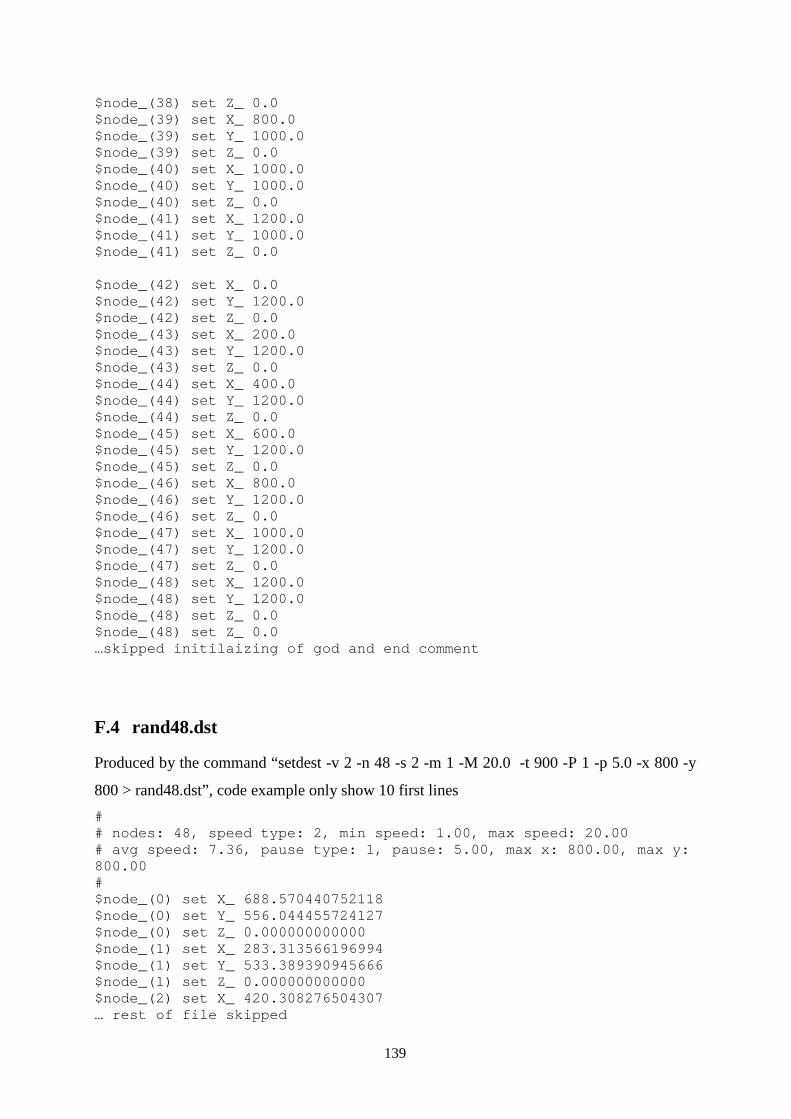
139
$node_(38) set Z_ 0.0 $node_(39) set X_ 800.0 $node_(39) set Y_ 1000.0 $node_(39) set Z_ 0.0 $node_(40) set X_ 1000.0 $node_(40) set Y_ 1000.0 $node_(40) set Z_ 0.0 $node_(41) set X_ 1200.0 $node_(41) set Y_ 1000.0 $node_(41) set Z_ 0.0
$node_(42) set X_ 0.0 $node_(42) set Y_ 1200.0 $node_(42) set Z_ 0.0 $node_(43) set X_ 200.0 $node_(43) set Y_ 1200.0 $node_(43) set Z_ 0.0 $node_(44) set X_ 400.0 $node_(44) set Y_ 1200.0 $node_(44) set Z_ 0.0 $node_(45) set X_ 600.0 $node_(45) set Y_ 1200.0 $node_(45) set Z_ 0.0 $node_(46) set X_ 800.0 $node_(46) set Y_ 1200.0 $node_(46) set Z_ 0.0 $node_(47) set X_ 1000.0 $node_(47) set Y_ 1200.0 $node_(47) set Z_ 0.0 $node_(48) set X_ 1200.0 $node_(48) set Y_ 1200.0 $node_(48) set Z_ 0.0 $node_(48) set Z_ 0.0 …skipped initilaizing of god and end comment
F.4 rand48.dst
Produced by the command “setdest -v 2 -n 48 -s 2 -m 1 -M 20.0 -t 900 -P 1 -p 5.0 -x 800 -y
800 > rand48.dst”, code example only show 10 first lines
# # nodes: 48, speed type: 2, min speed: 1.00, max sp eed: 20.00 # avg speed: 7.36, pause type: 1, pause: 5.00, max x: 800.00, max y: 800.00 # $node_(0) set X_ 688.570440752118 $node_(0) set Y_ 556.044455724127 $node_(0) set Z_ 0.000000000000 $node_(1) set X_ 283.313566196994 $node_(1) set Y_ 533.389390945666 $node_(1) set Z_ 0.000000000000 $node_(2) set X_ 420.308276504307 … rest of file skipped
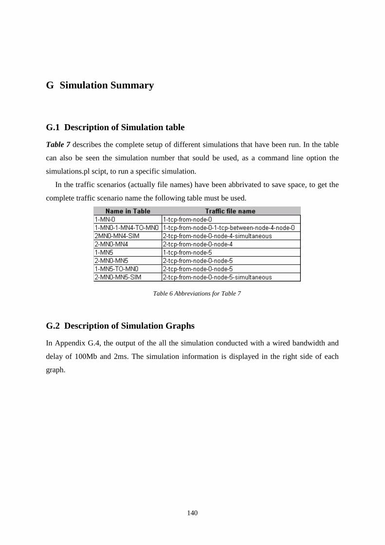
140
G Simulation Summary
G.1 Description of Simulation table
Table 7 describes the complete setup of different simulations that have been run. In the table
can also be seen the simulation number that sould be used, as a command line option the
simulations.pl scipt, to run a specific simulation.
In the traffic scenarios (actually file names) have been abbrivated to save space, to get the
complete traffic scenario name the following table must be used.
Table 6 Abbreviations for Table 7
G.2 Description of Simulation Graphs
In Appendix G.4, the output of the all the simulation conducted with a wired bandwidth and
delay of 100Mb and 2ms. The simulation information is displayed in the right side of each
graph.
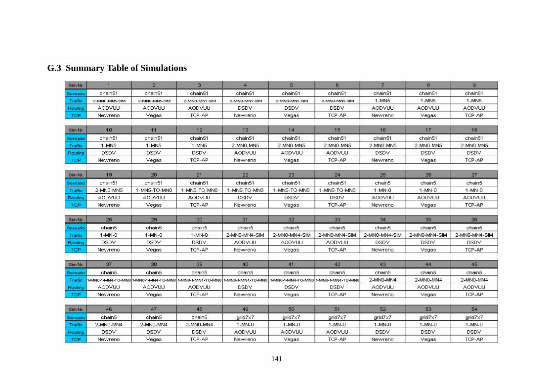
141
G.3 Summary Table of Simulations
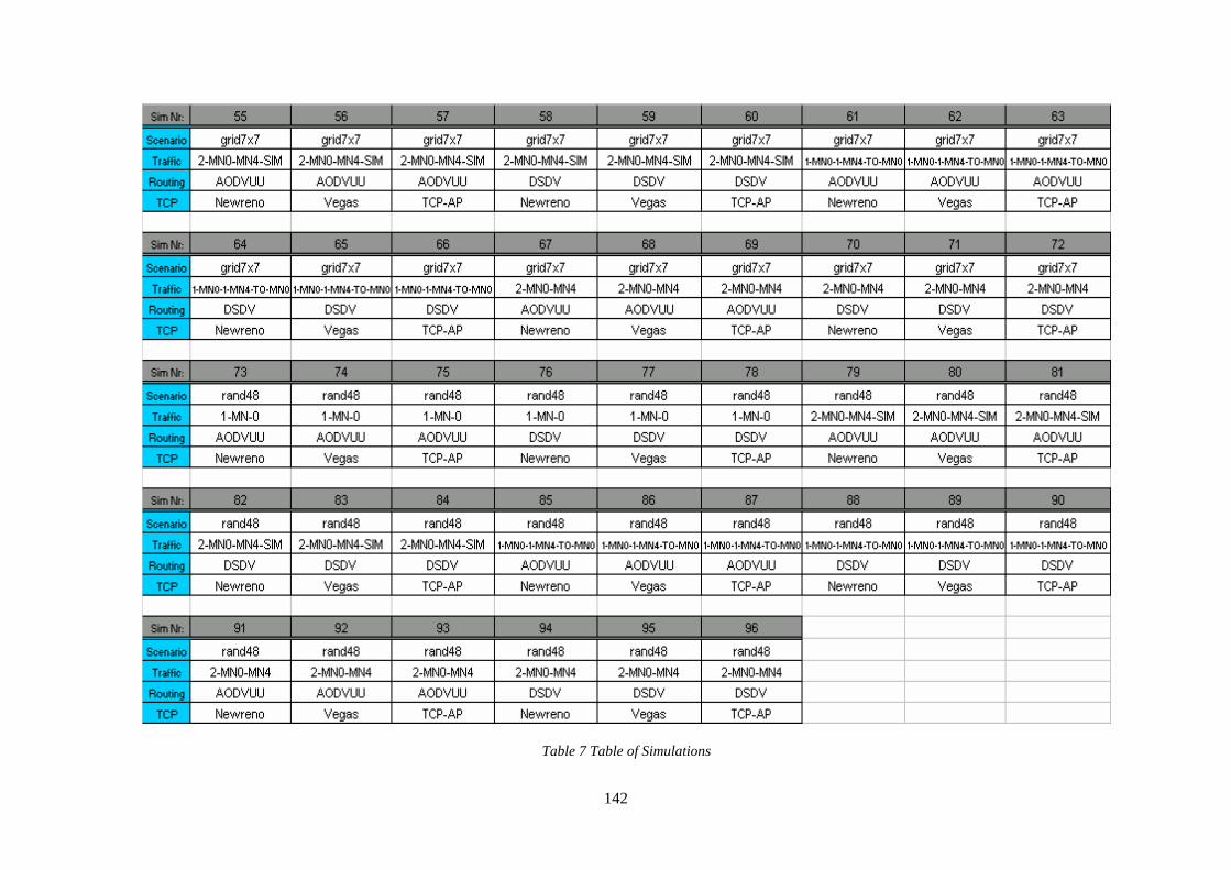
142
Table 7 Table of Simulations
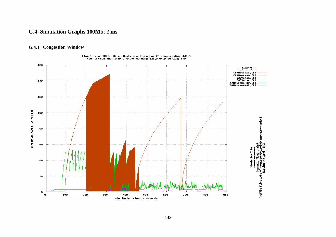
143
G.4 Simulation Graphs 100Mb, 2 ms
G.4.1 Congestion Window
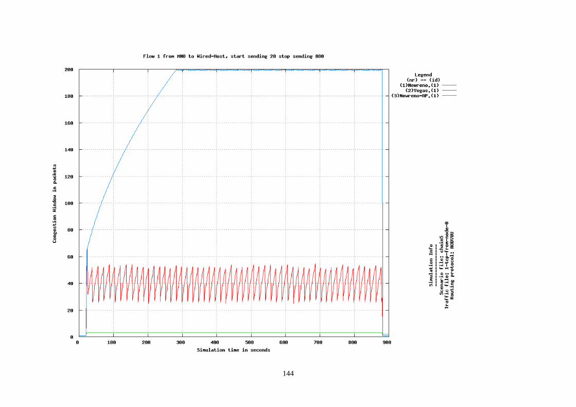
144
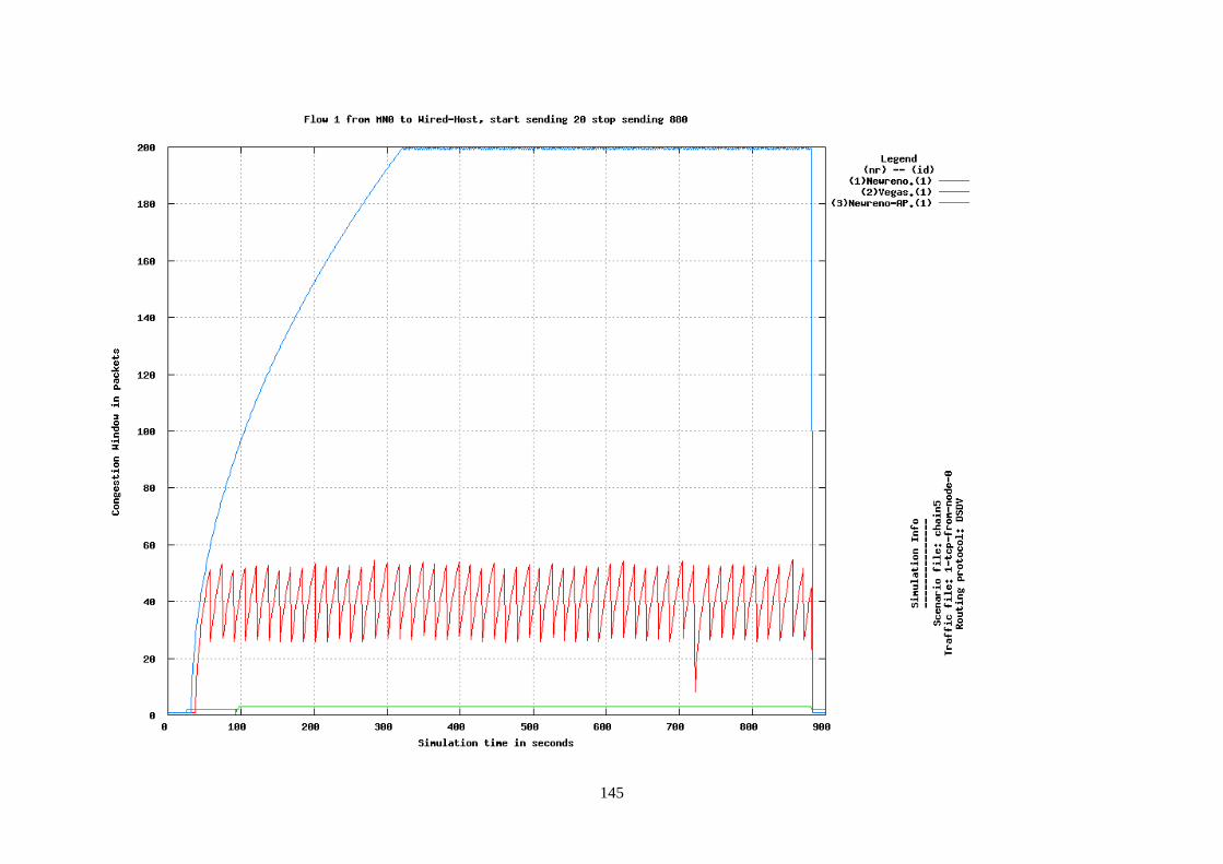
145
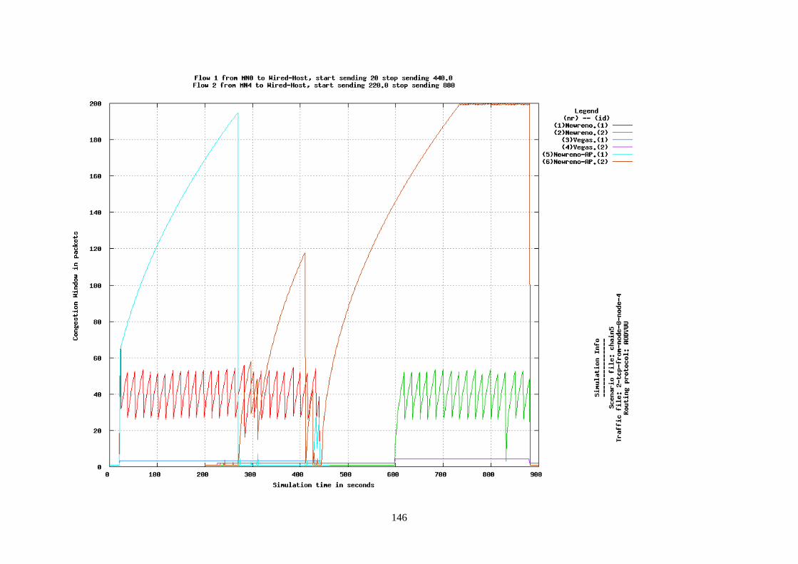
146
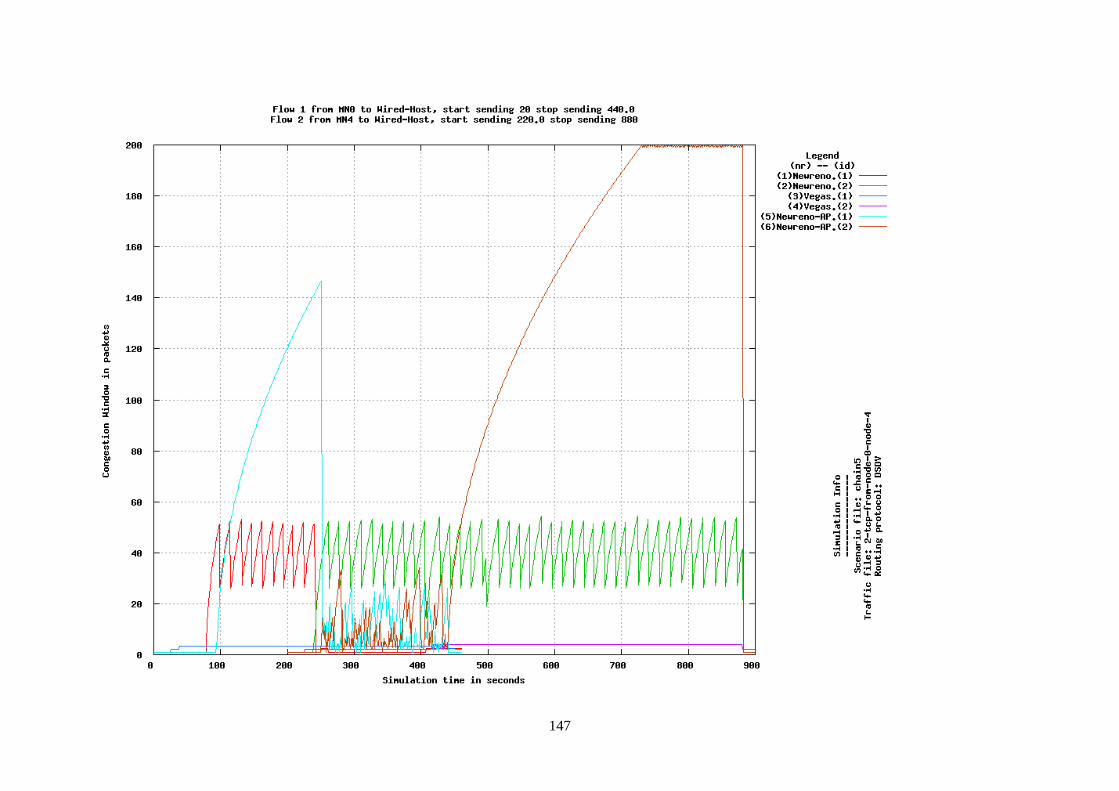
147
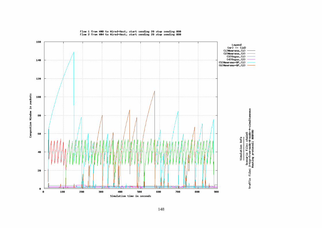
148
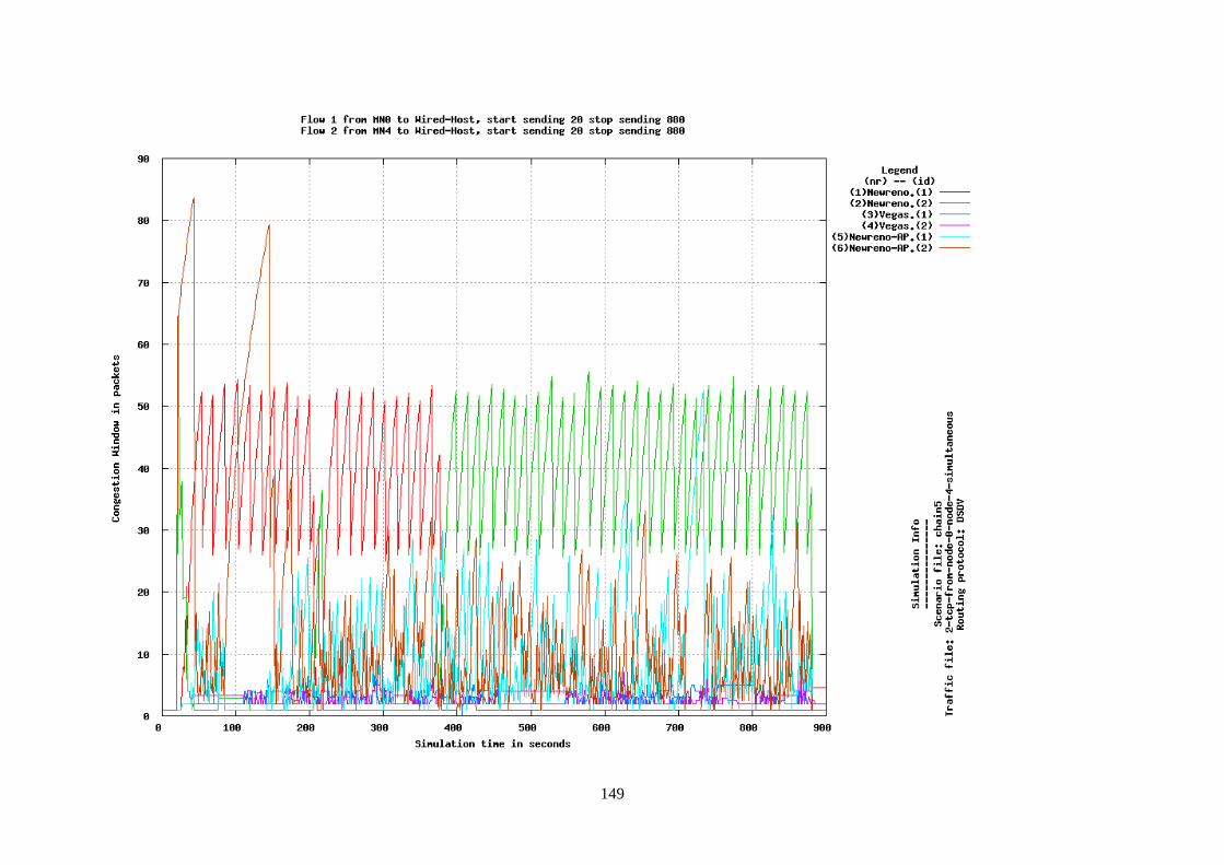
149
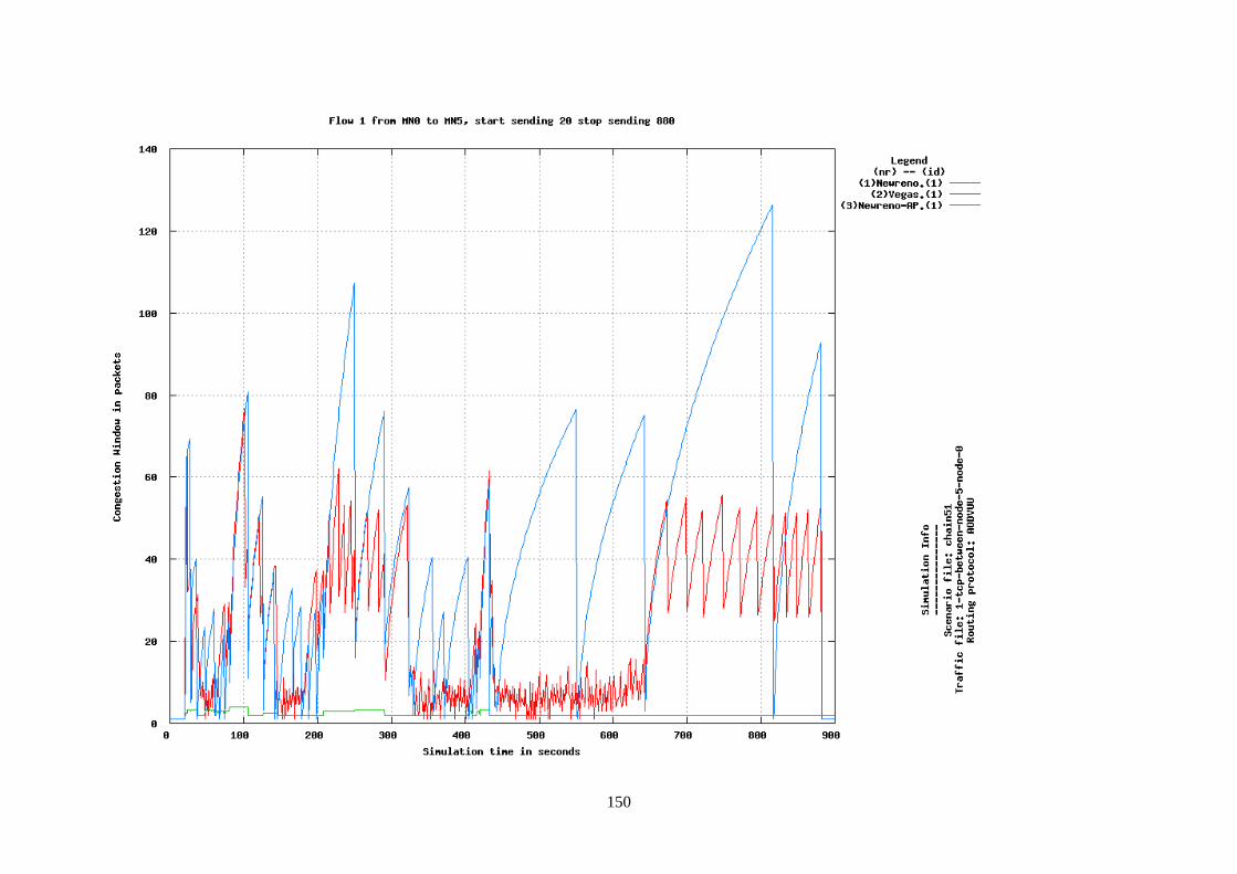
150
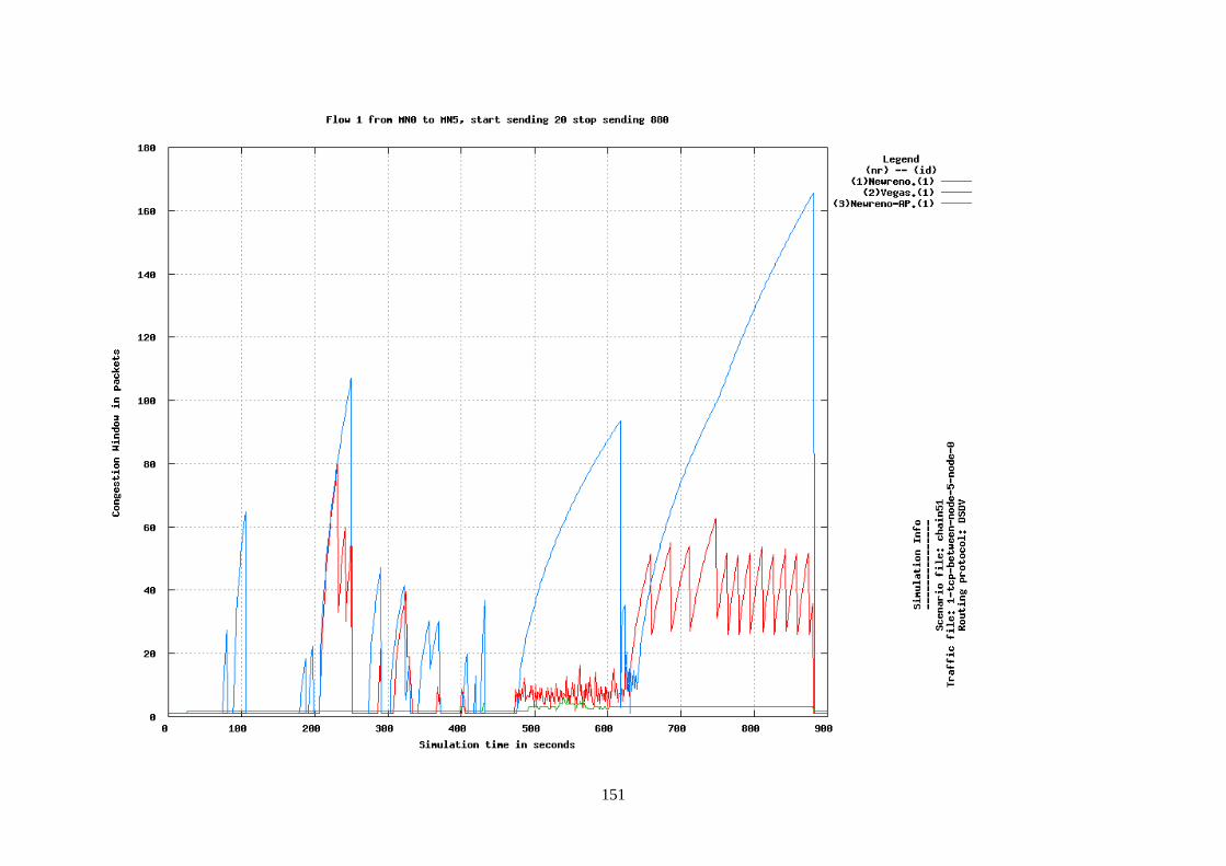
151
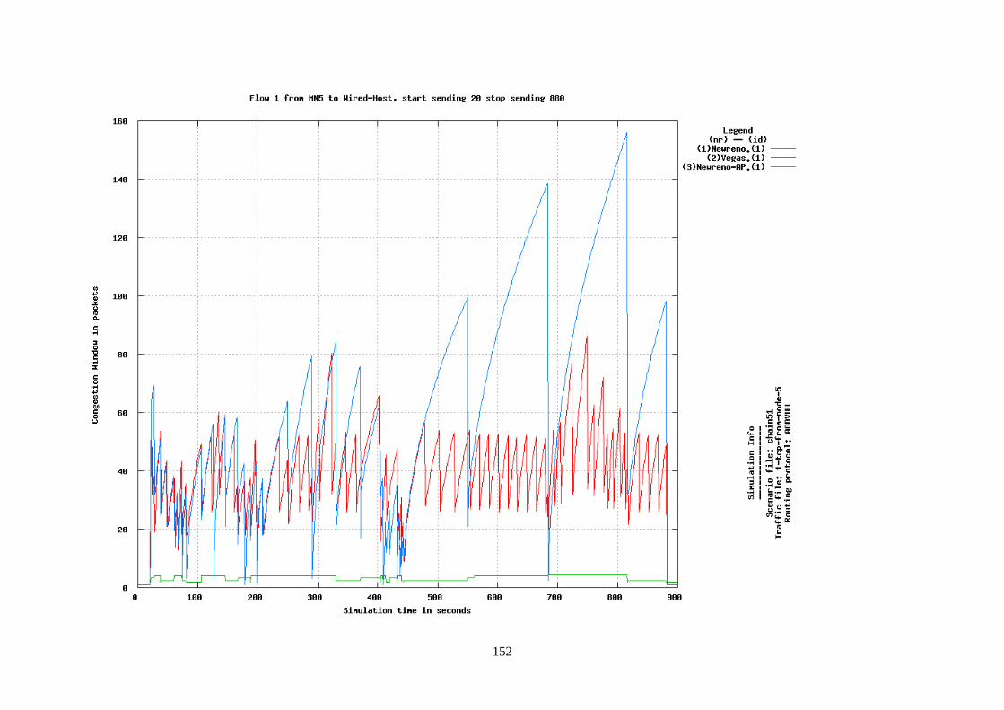
152
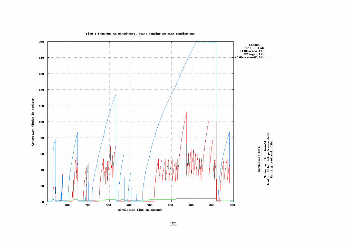
153
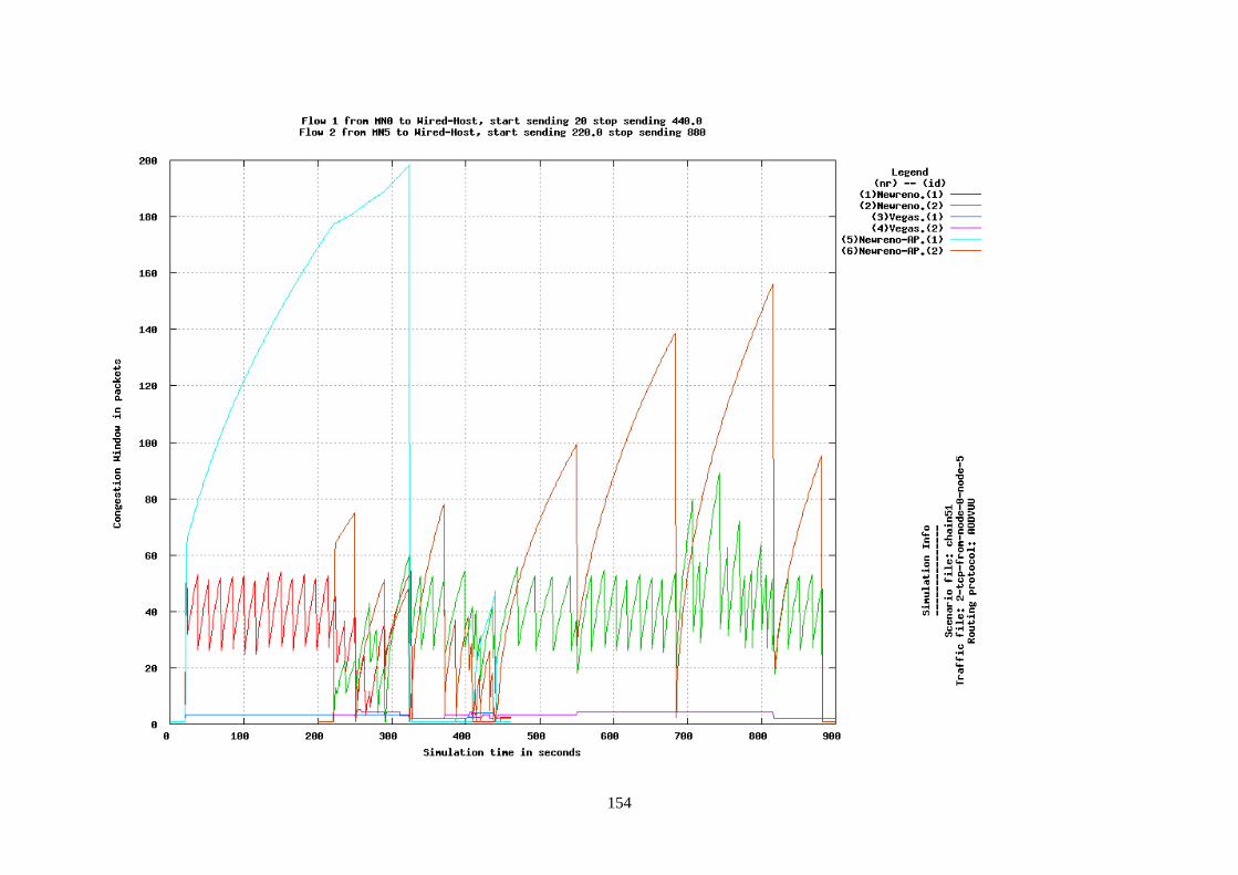
154
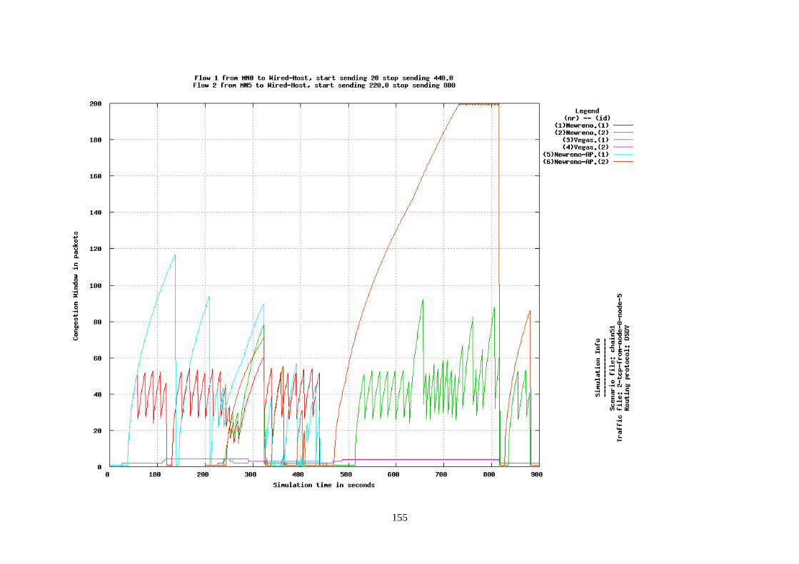
155
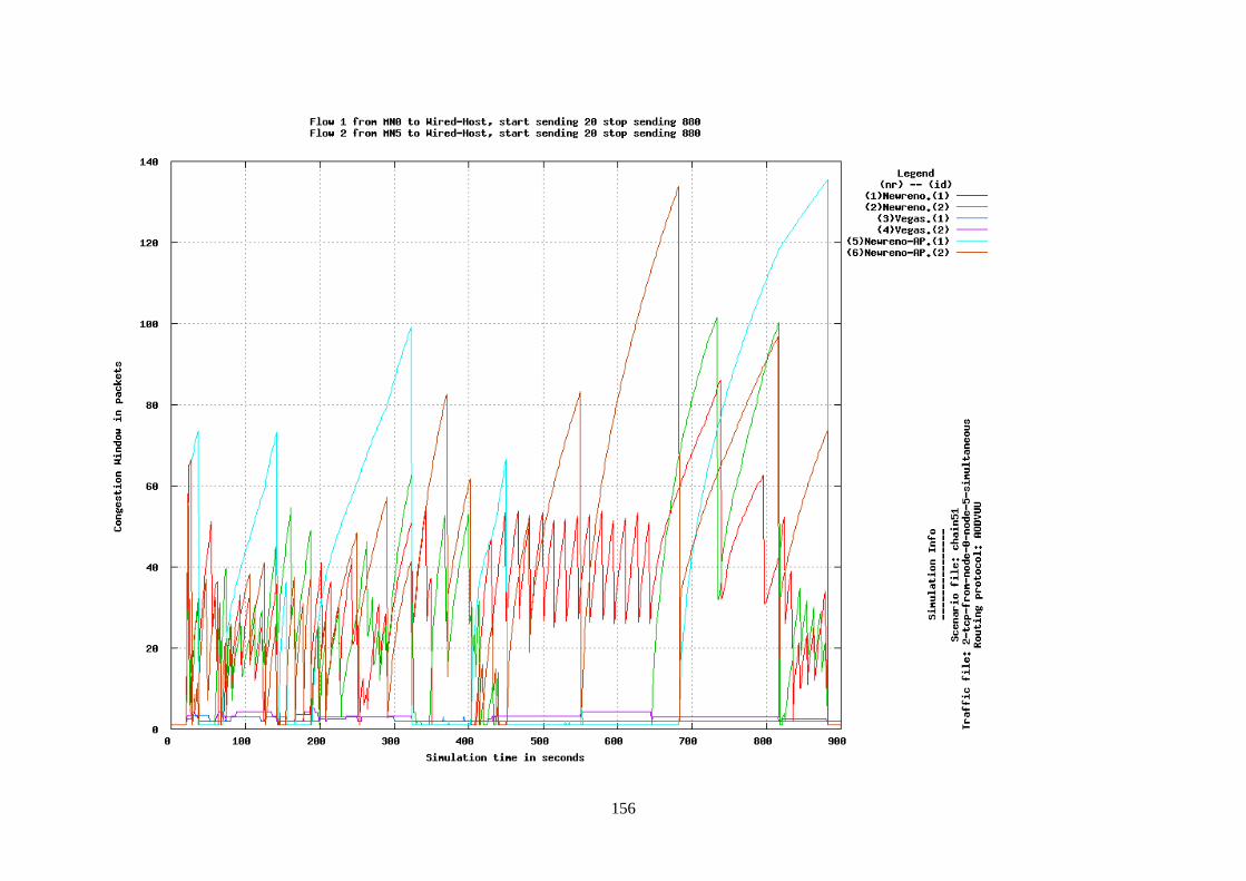
156
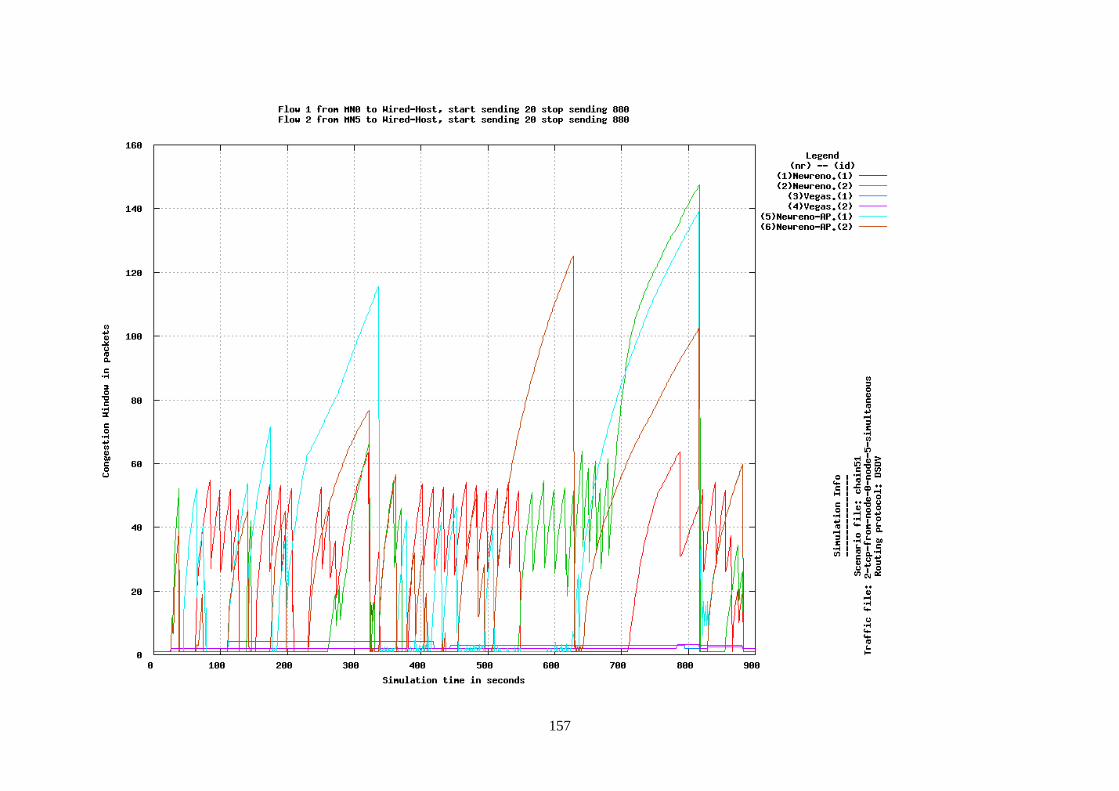
157
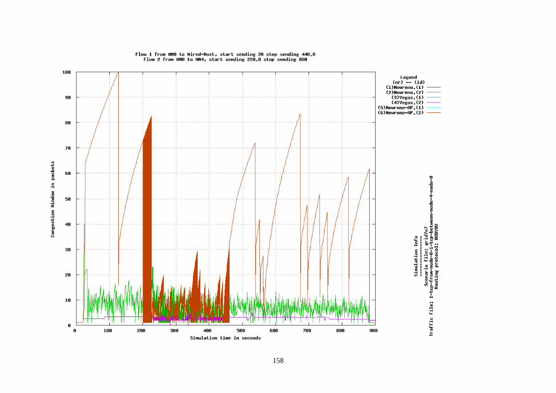
158
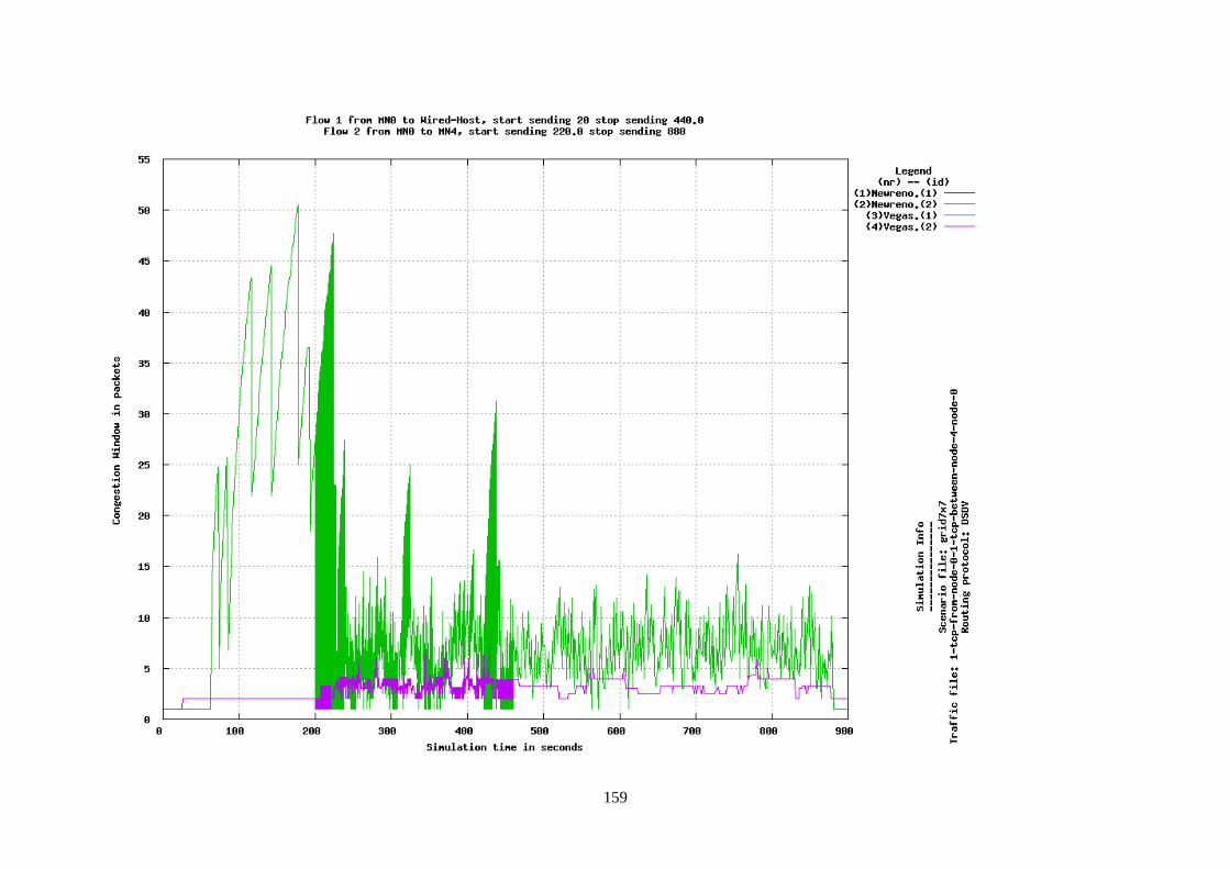
159
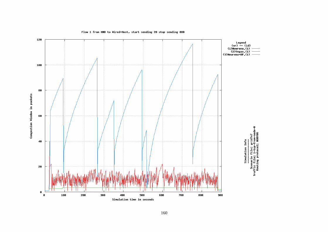
160
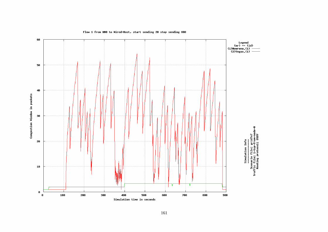
161
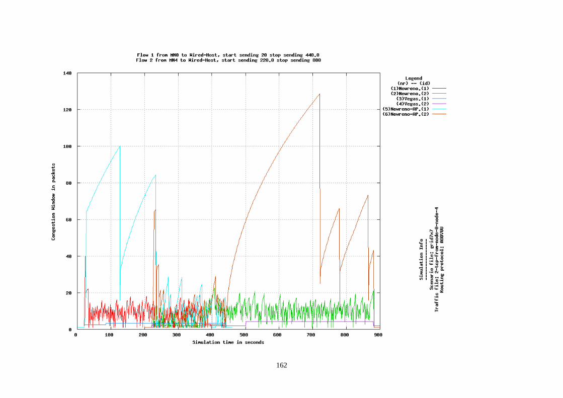
162
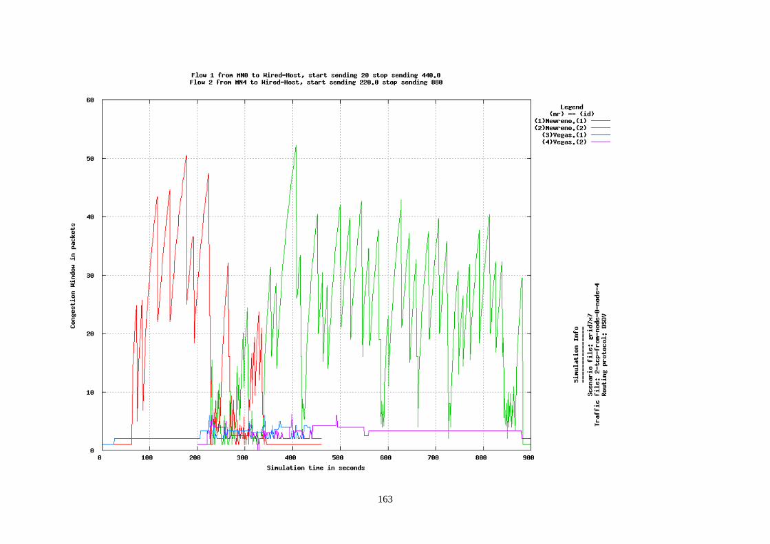
163
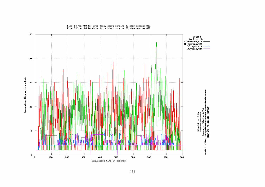
164
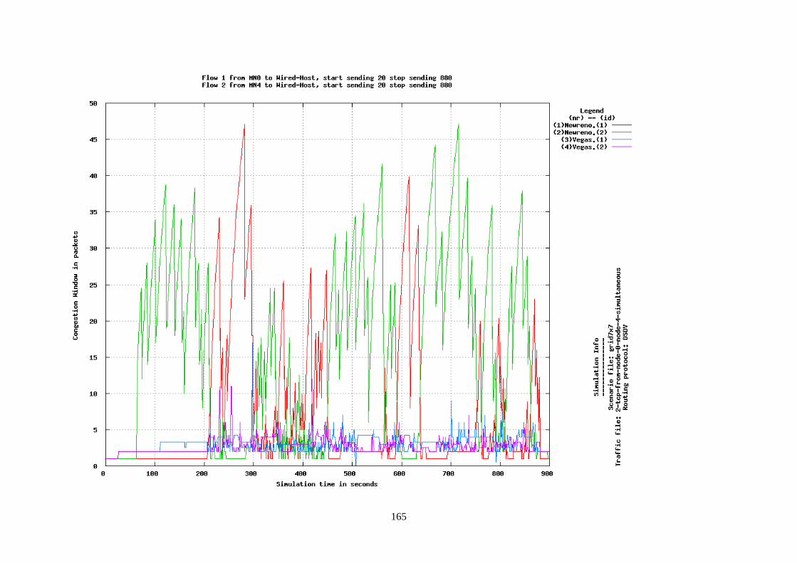
165
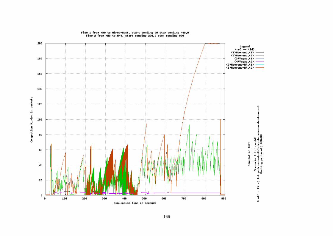
166
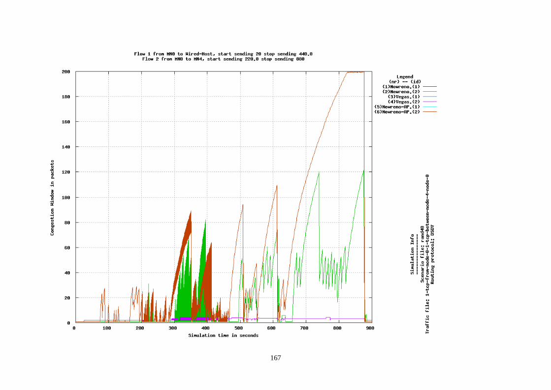
167
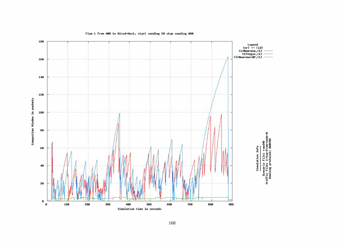
168
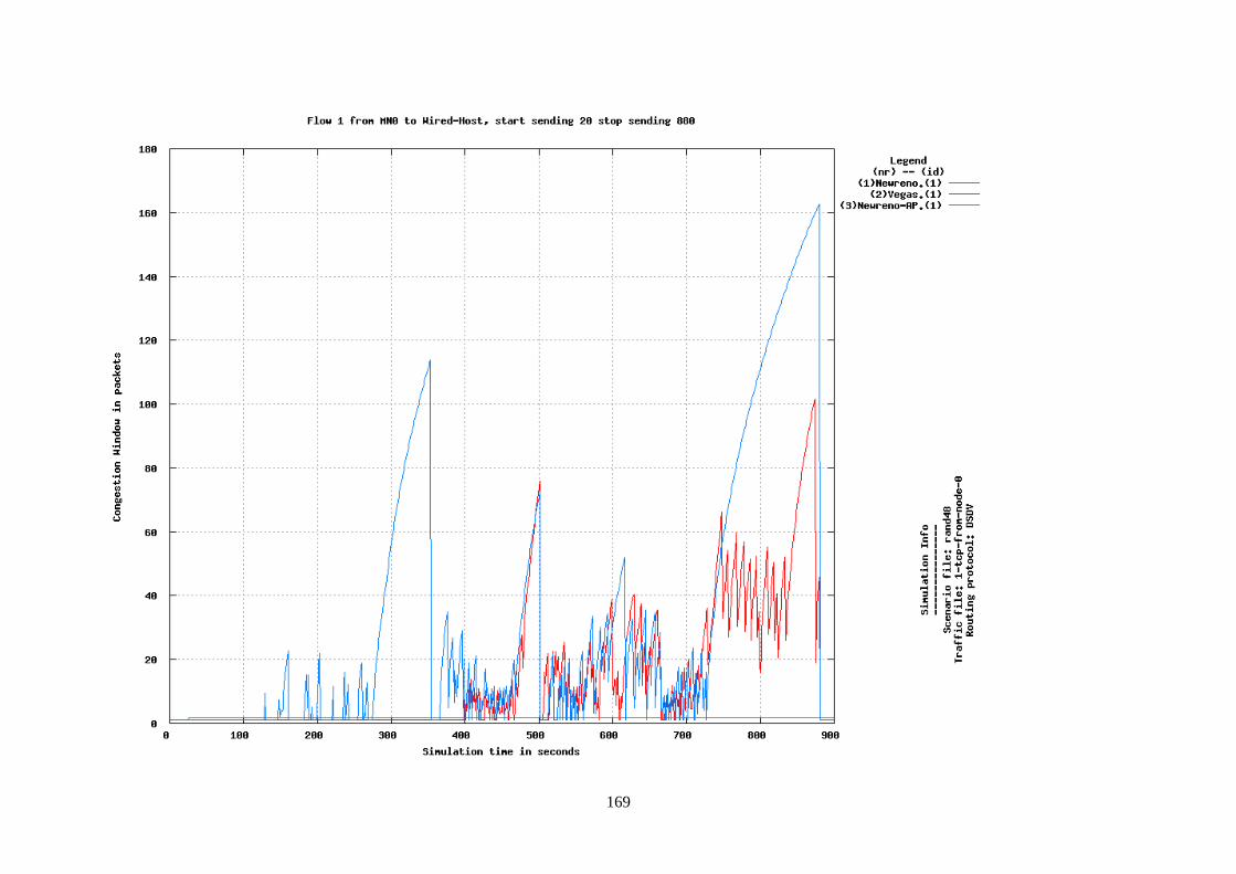
169
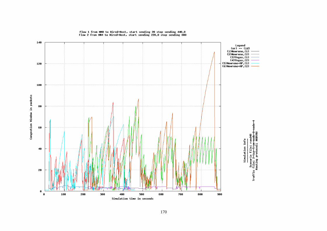
170
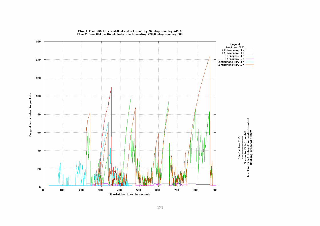
171
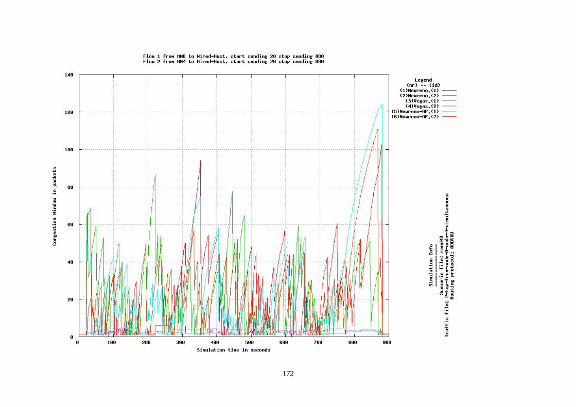
172
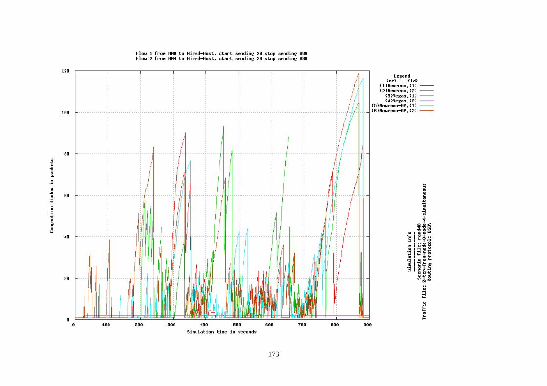
173
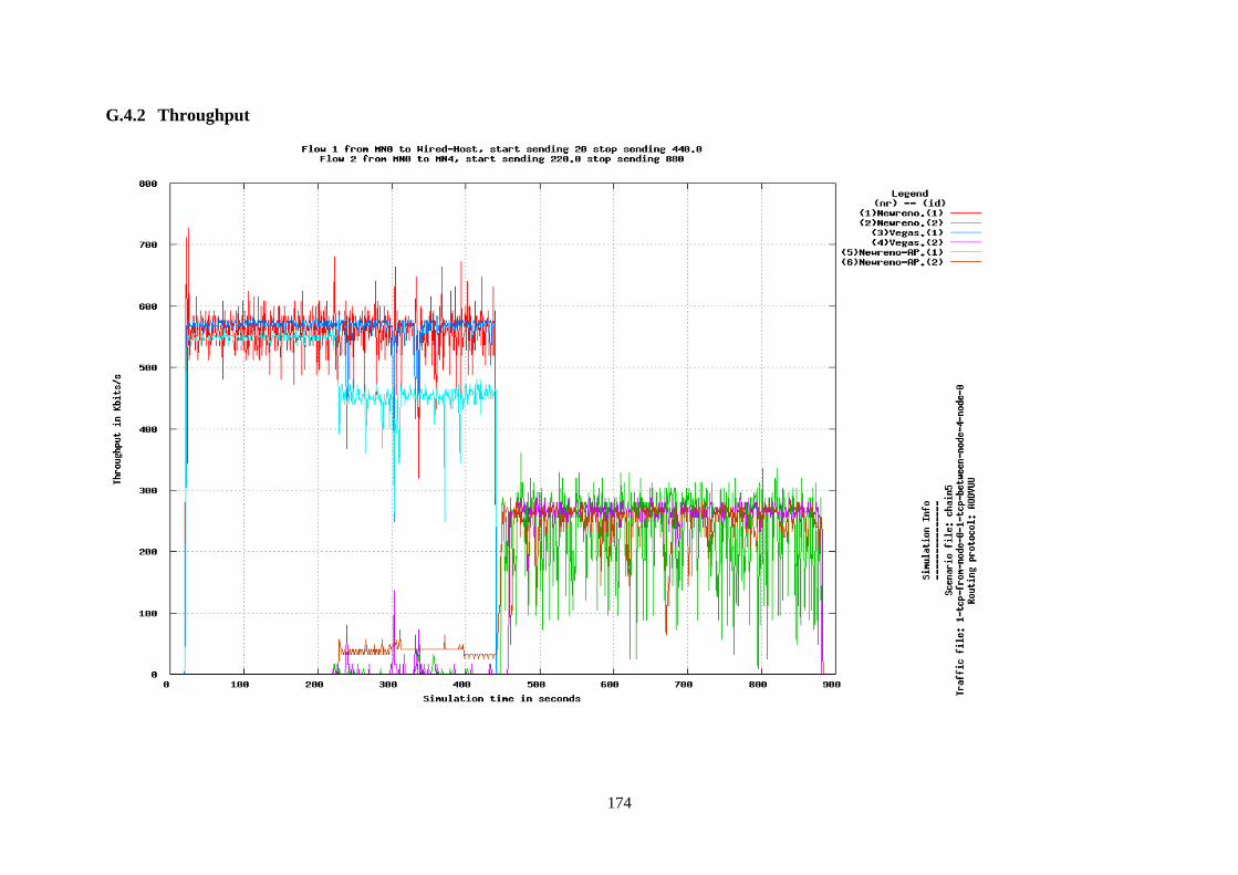
174
G.4.2 Throughput
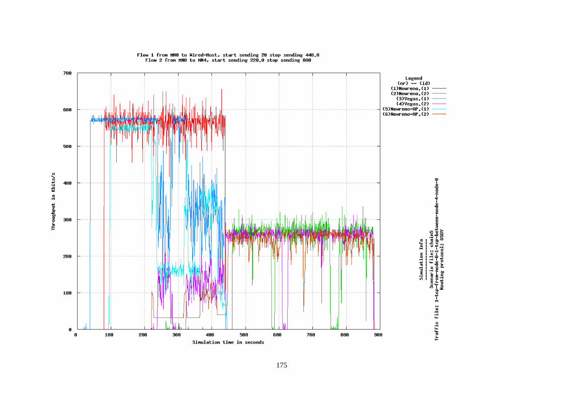
175

176
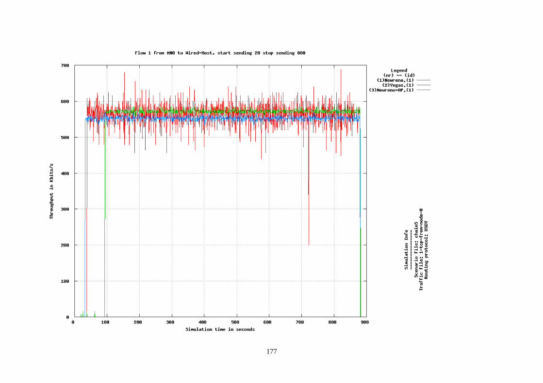
177
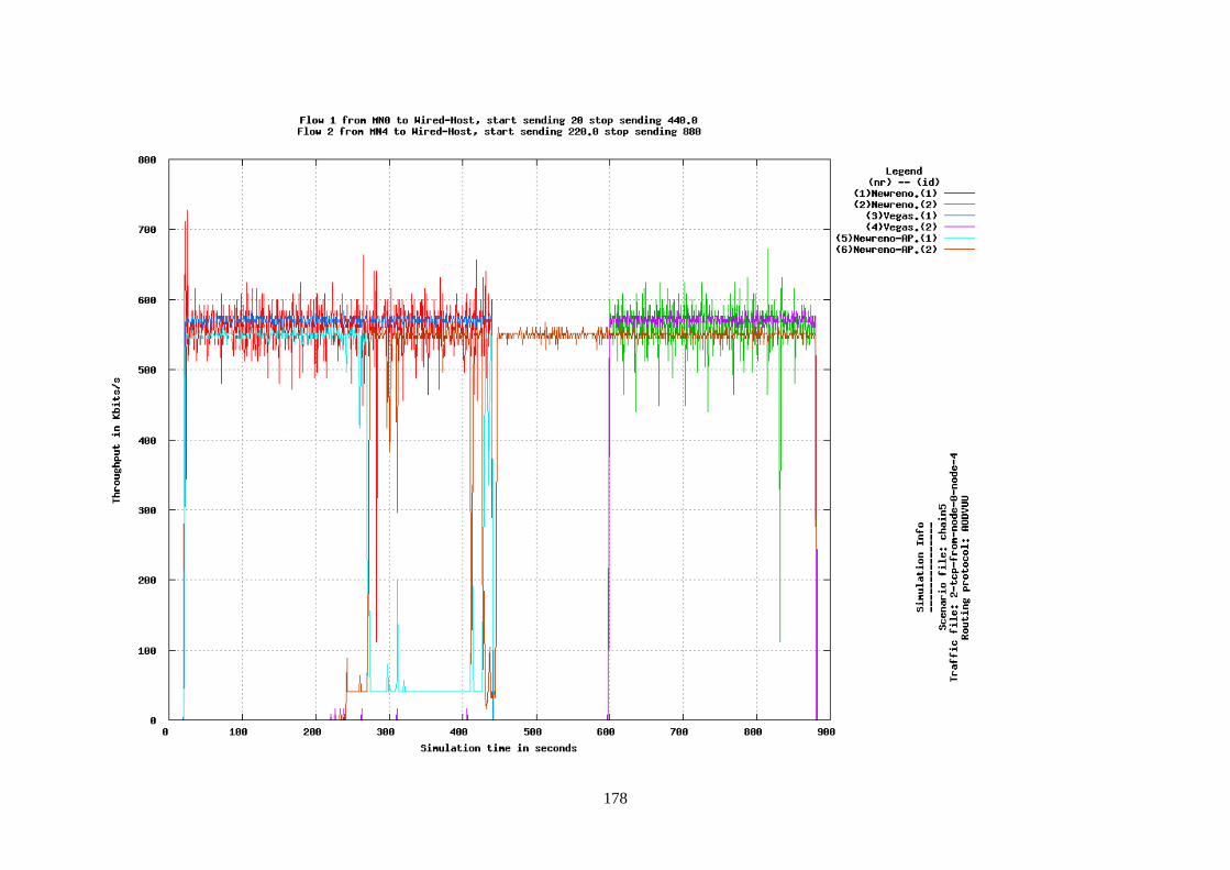
178
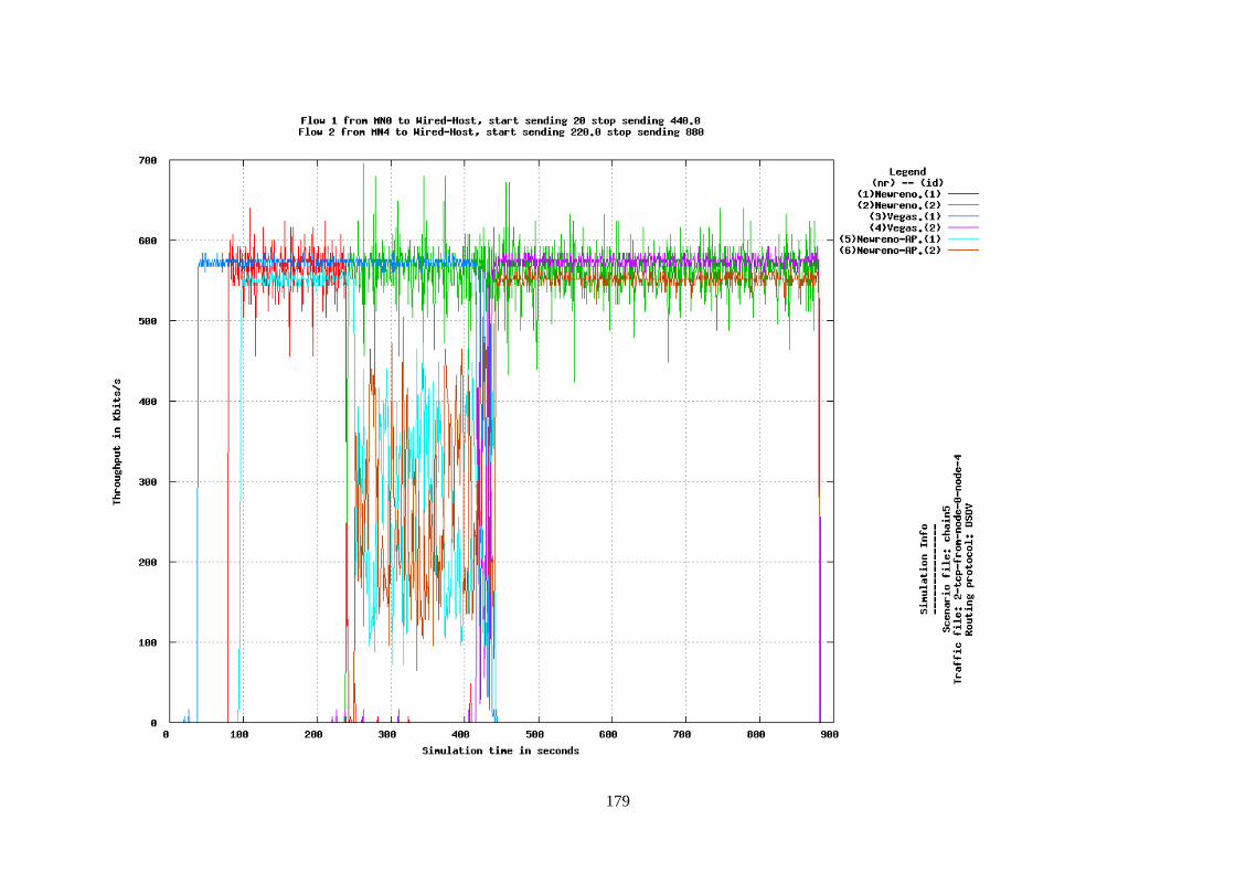
179
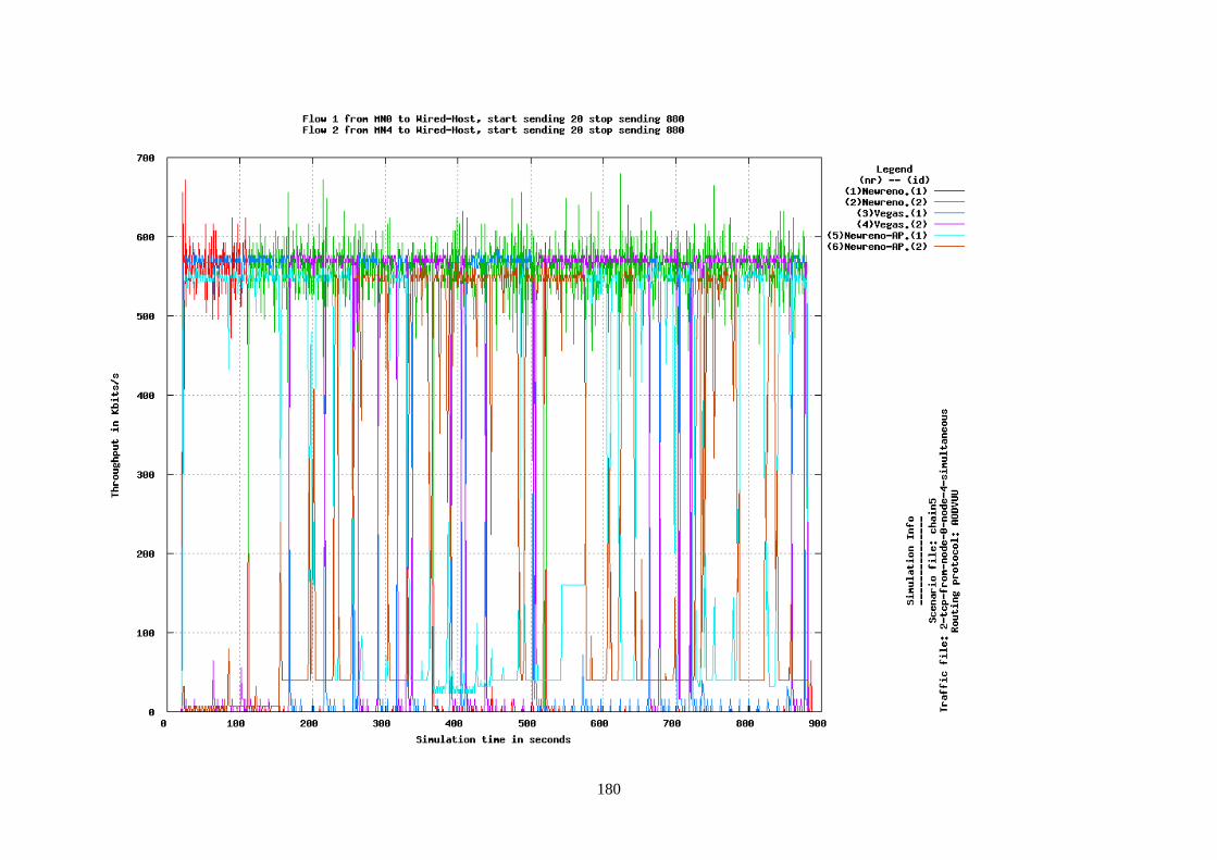
180
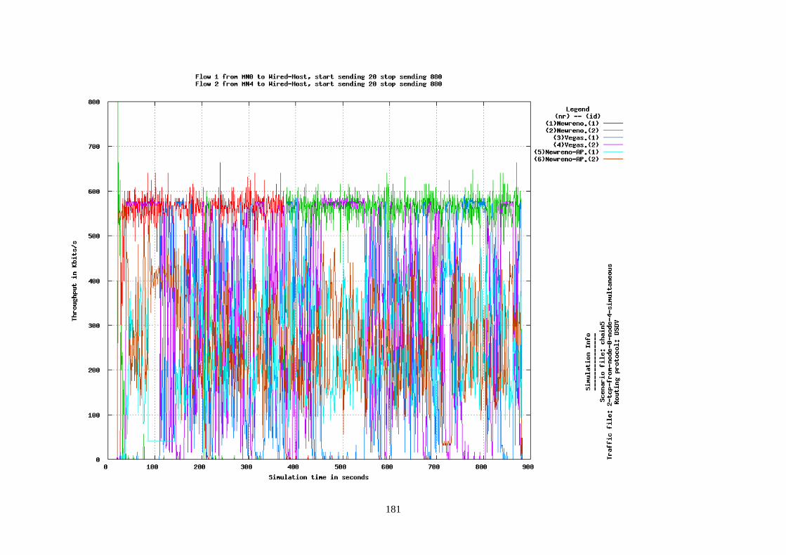
181
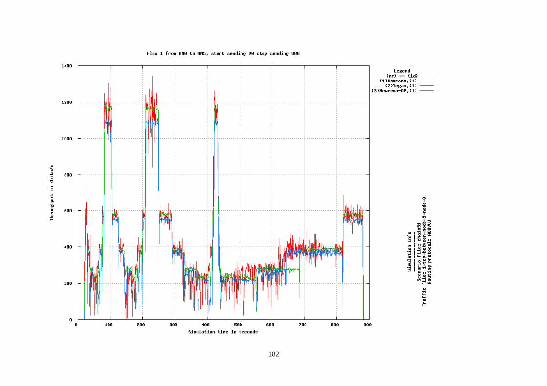
182
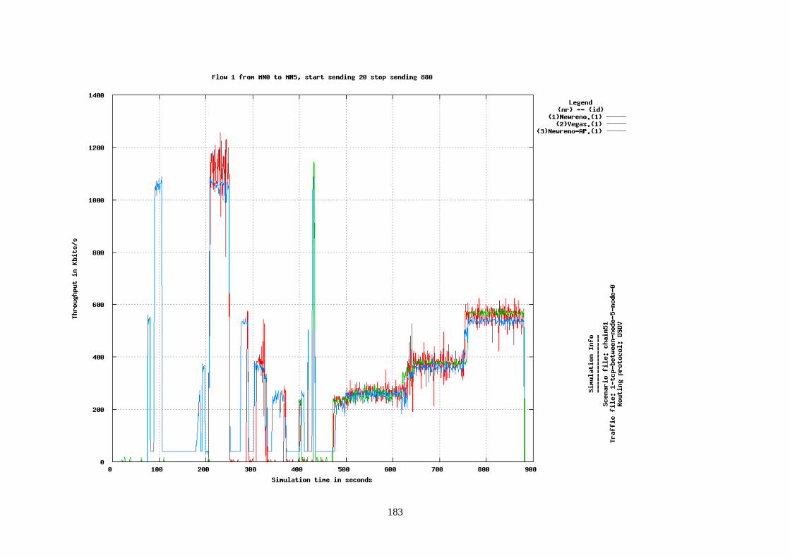
183
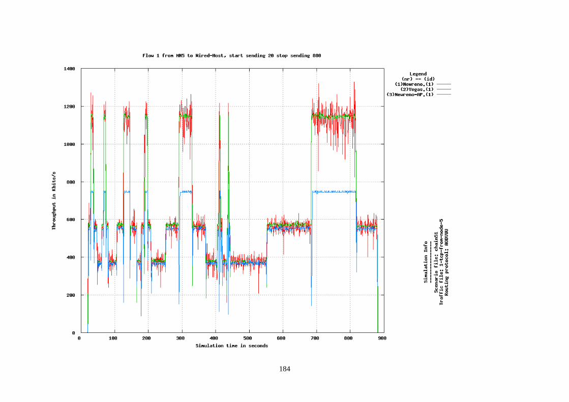
184
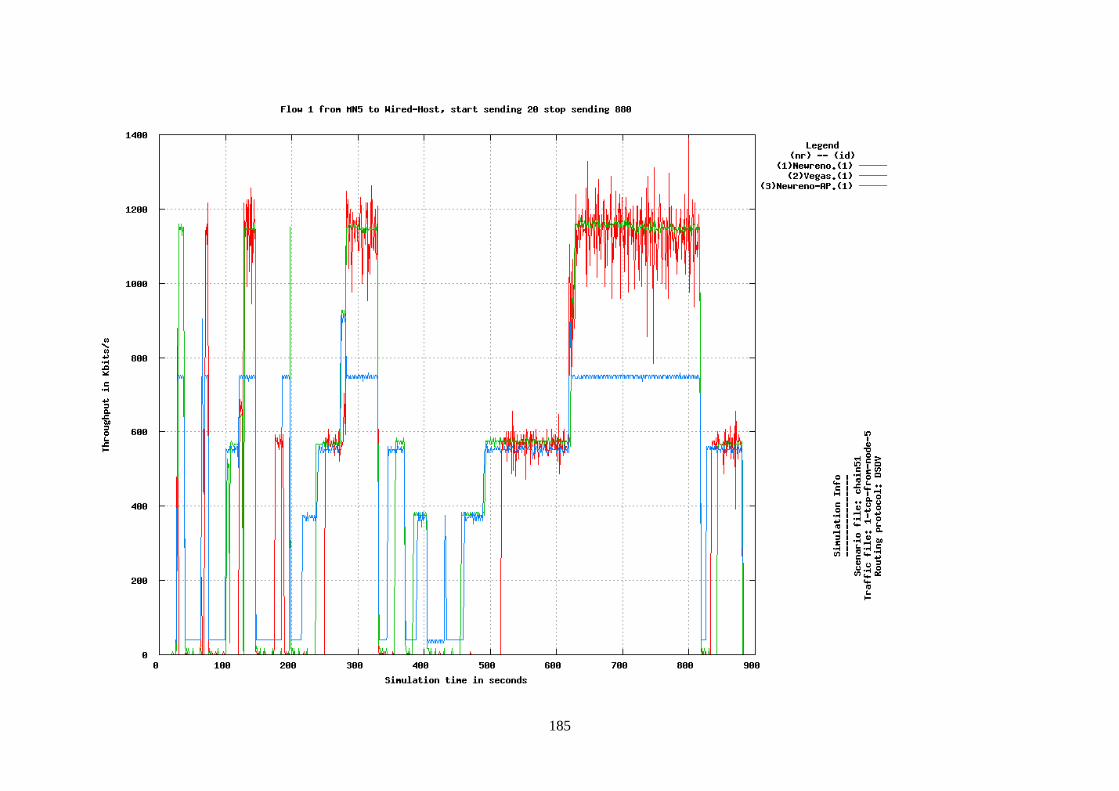
185
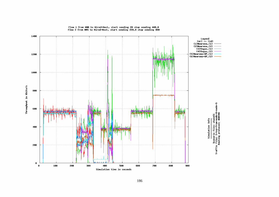
186

187
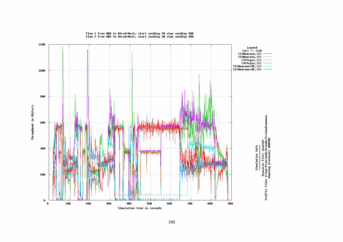
188
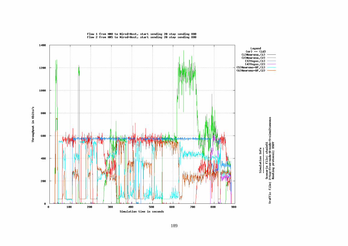
189
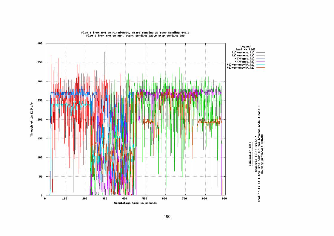
190
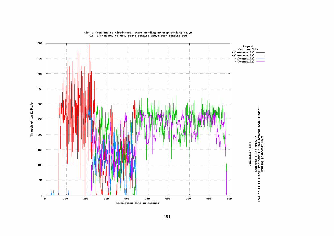
191
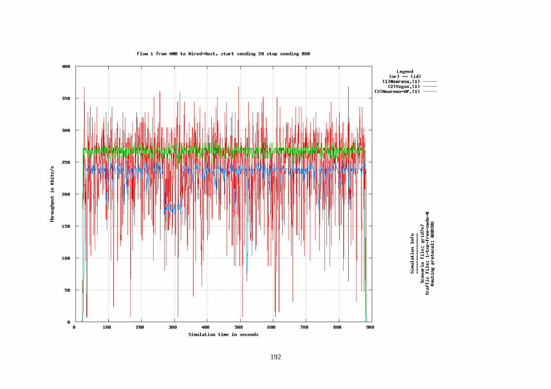
192
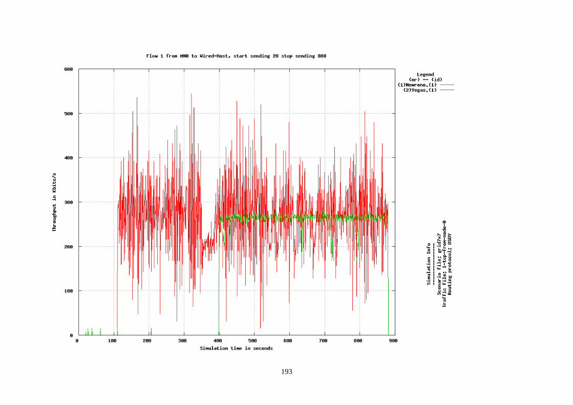
193
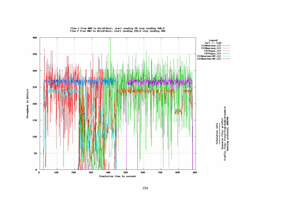
194
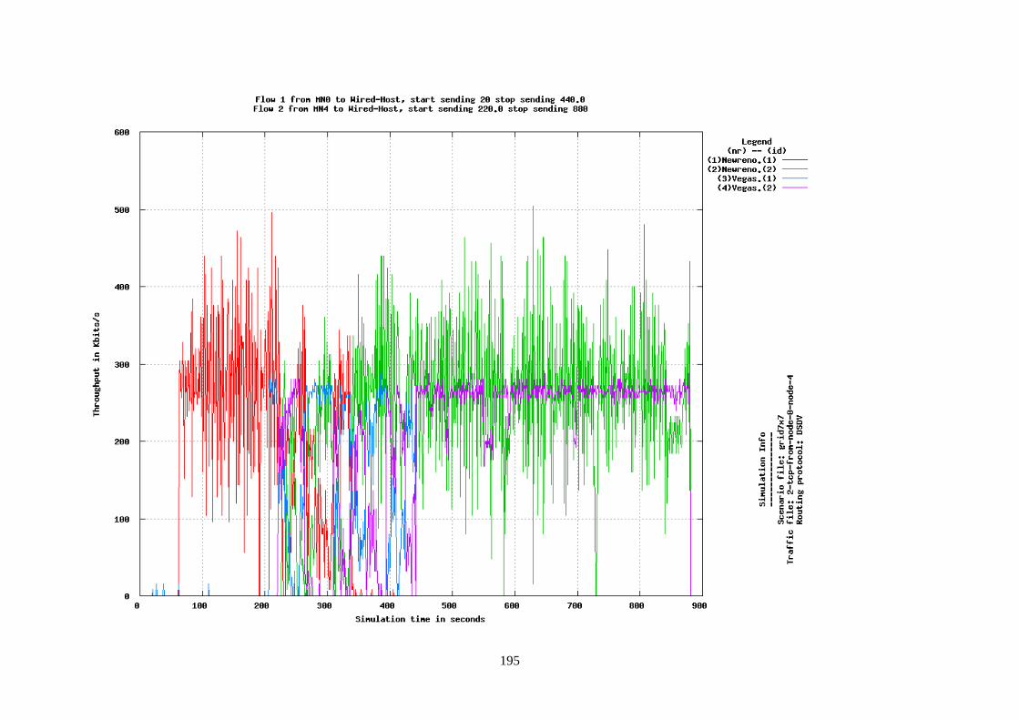
195
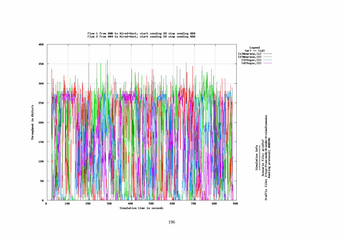
196
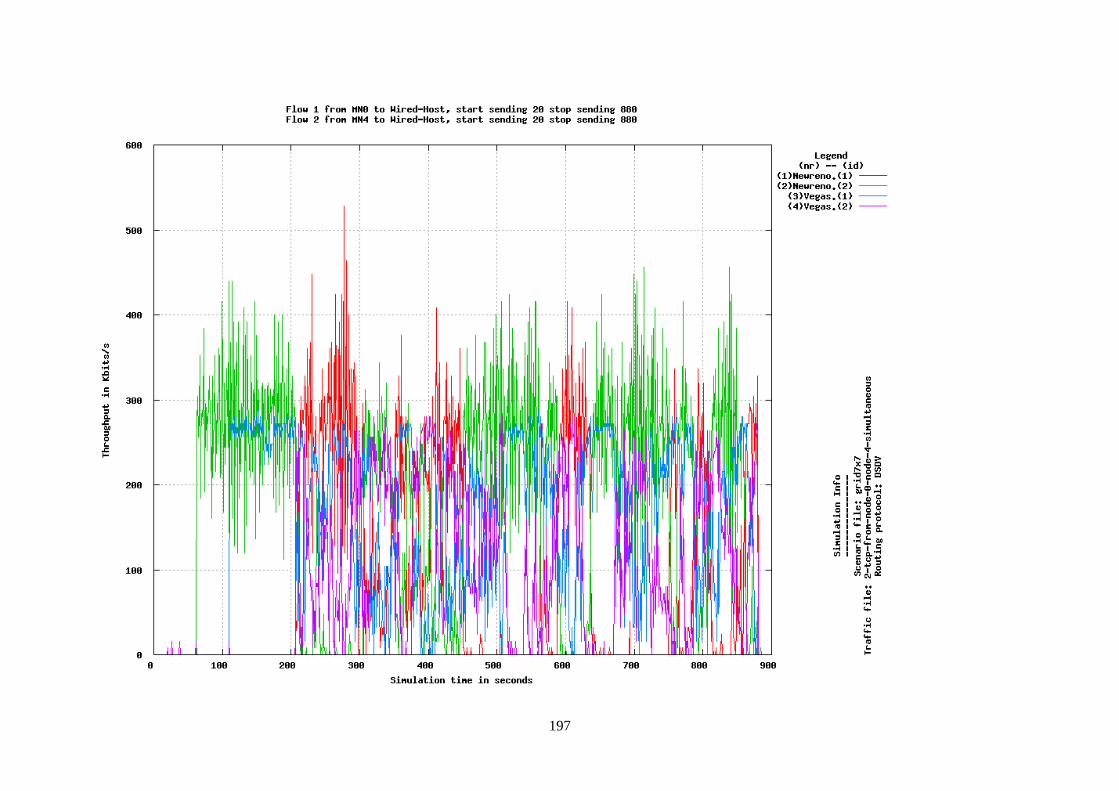
197
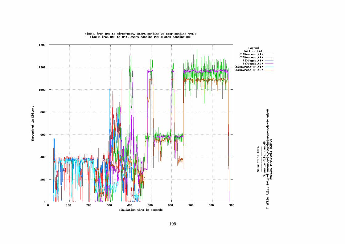
198
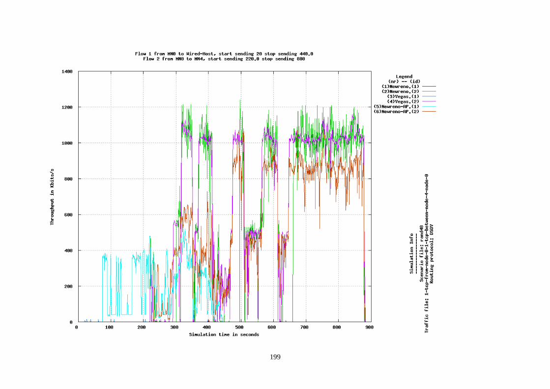
199
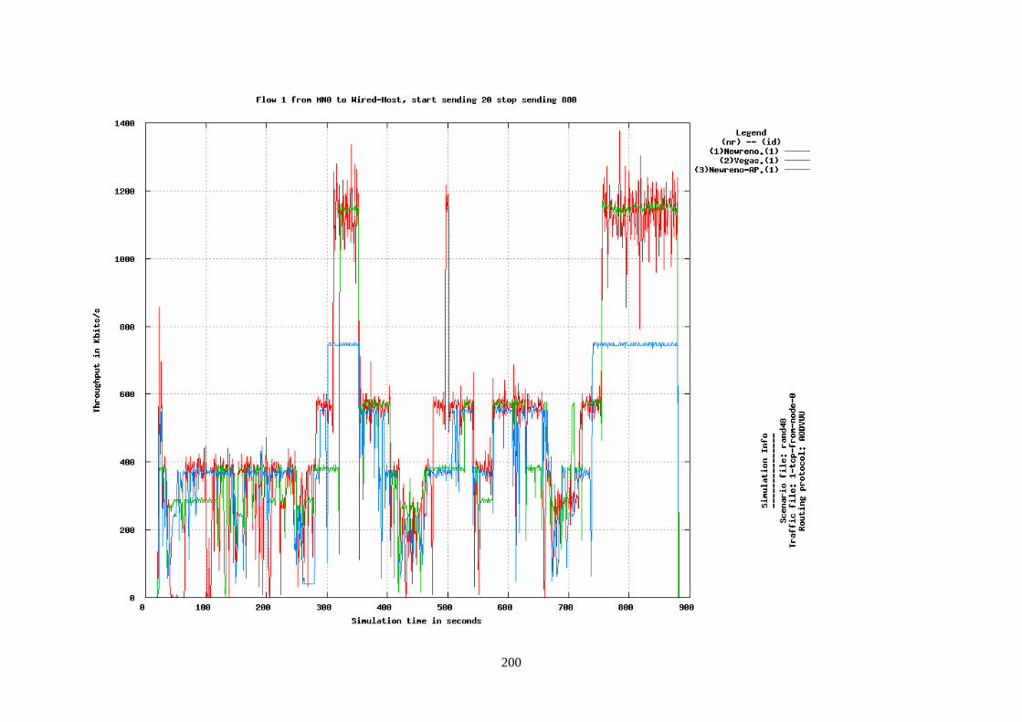
200
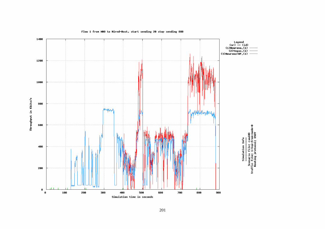
201
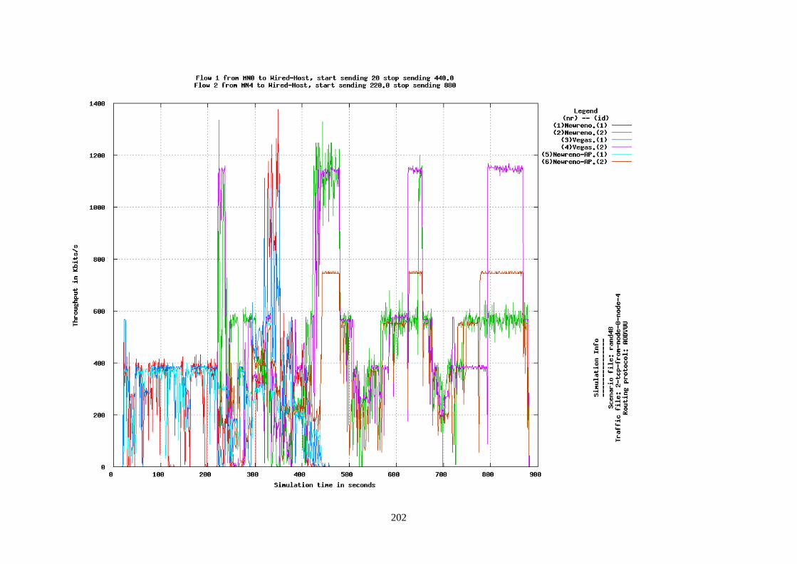
202

203
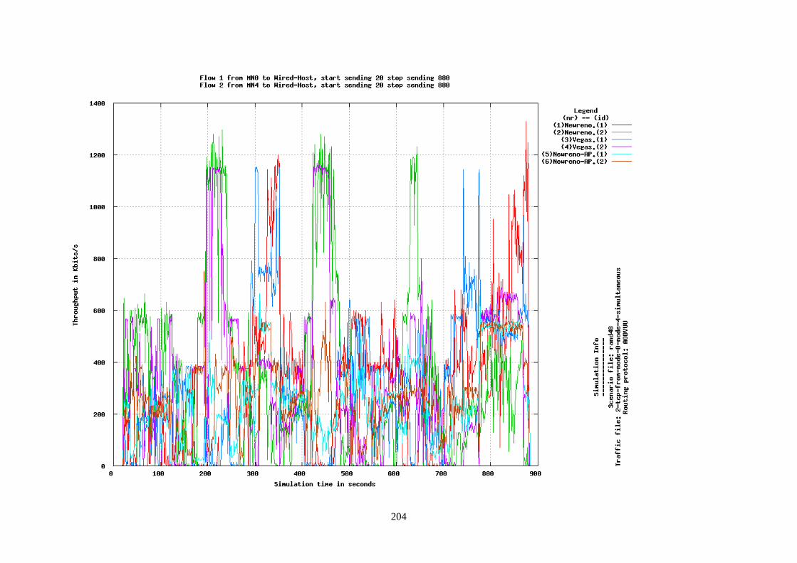
204
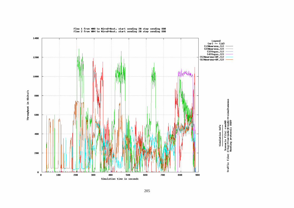
205
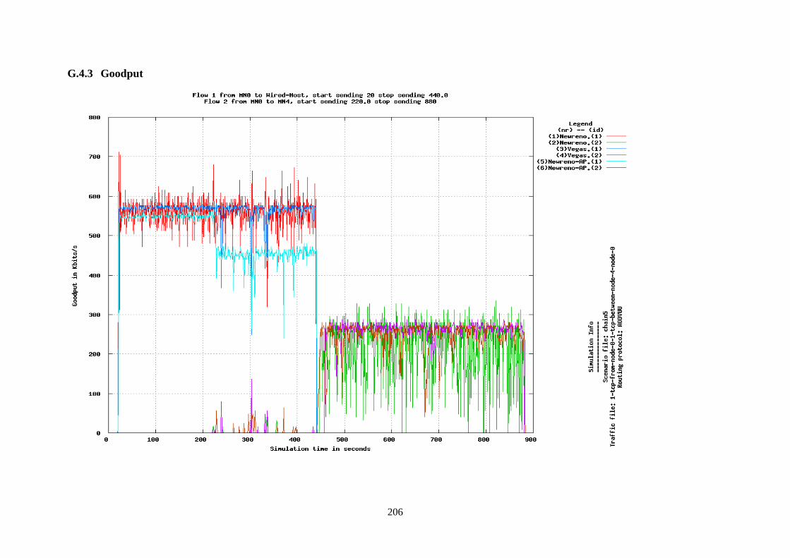
206
G.4.3 Goodput

207

208

209
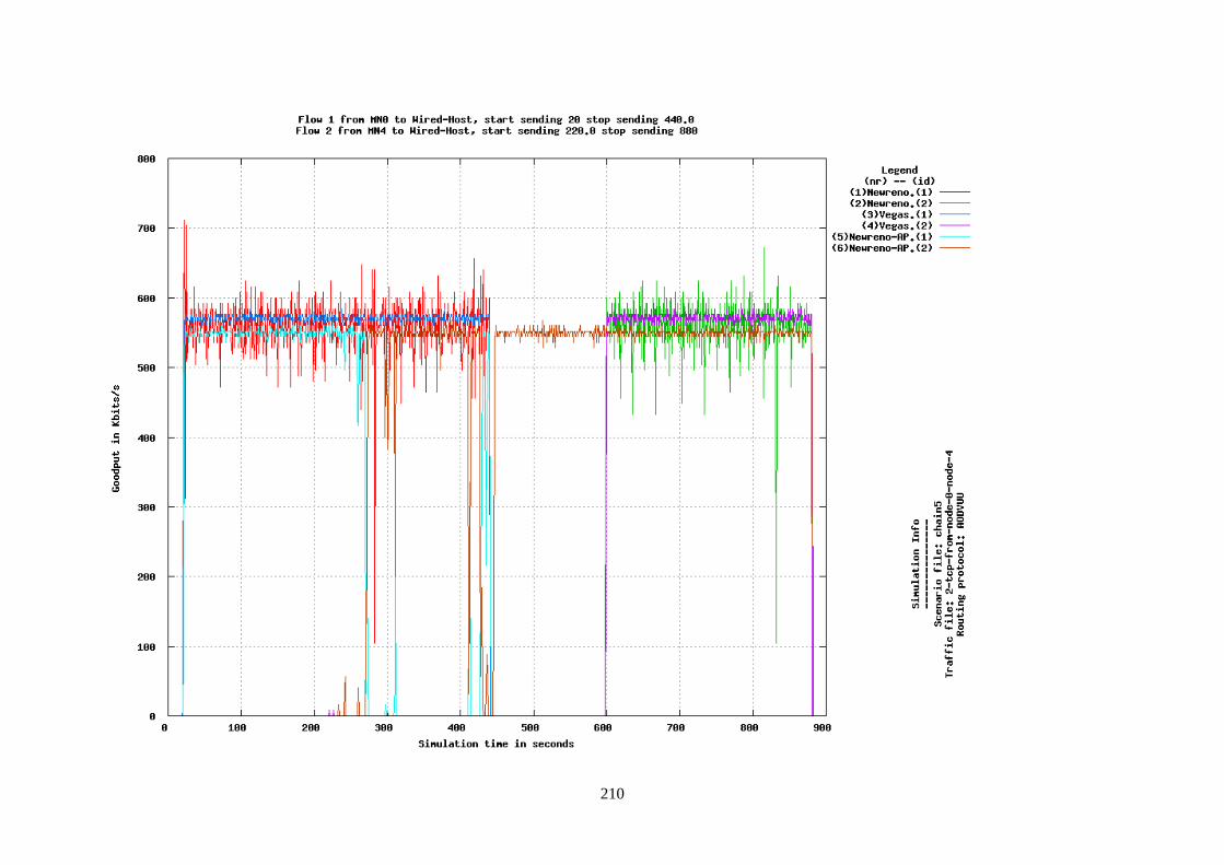
210
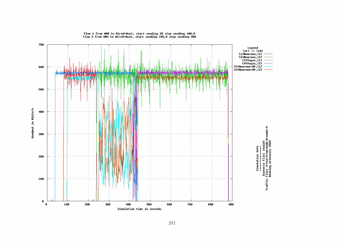
211
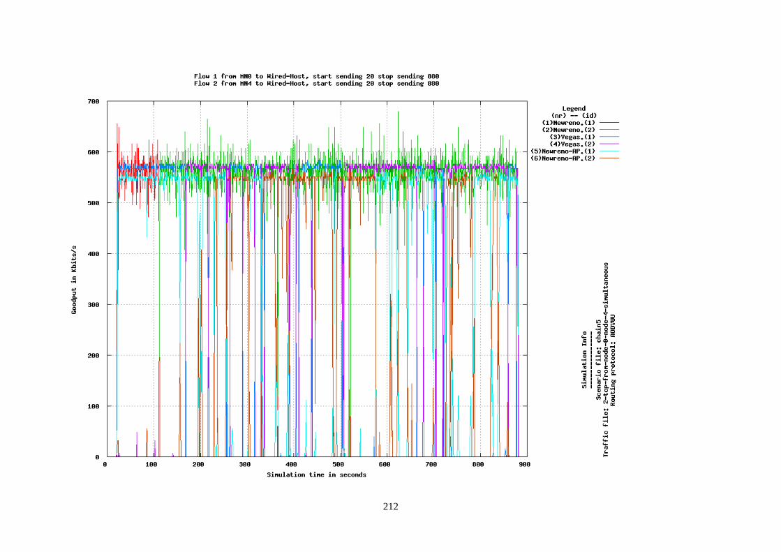
212
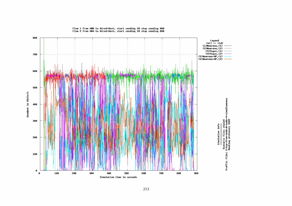
213
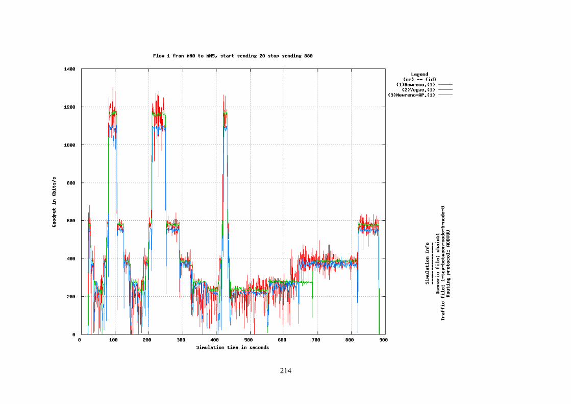
214
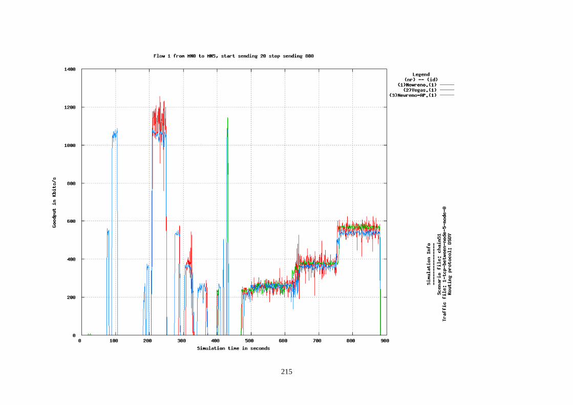
215
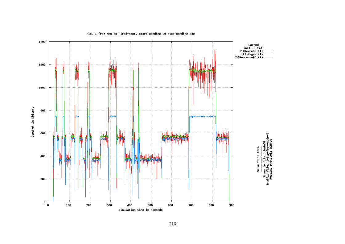
216
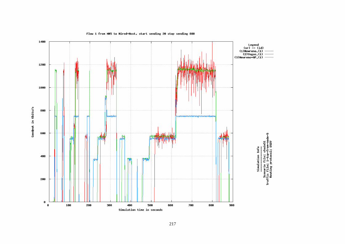
217

218
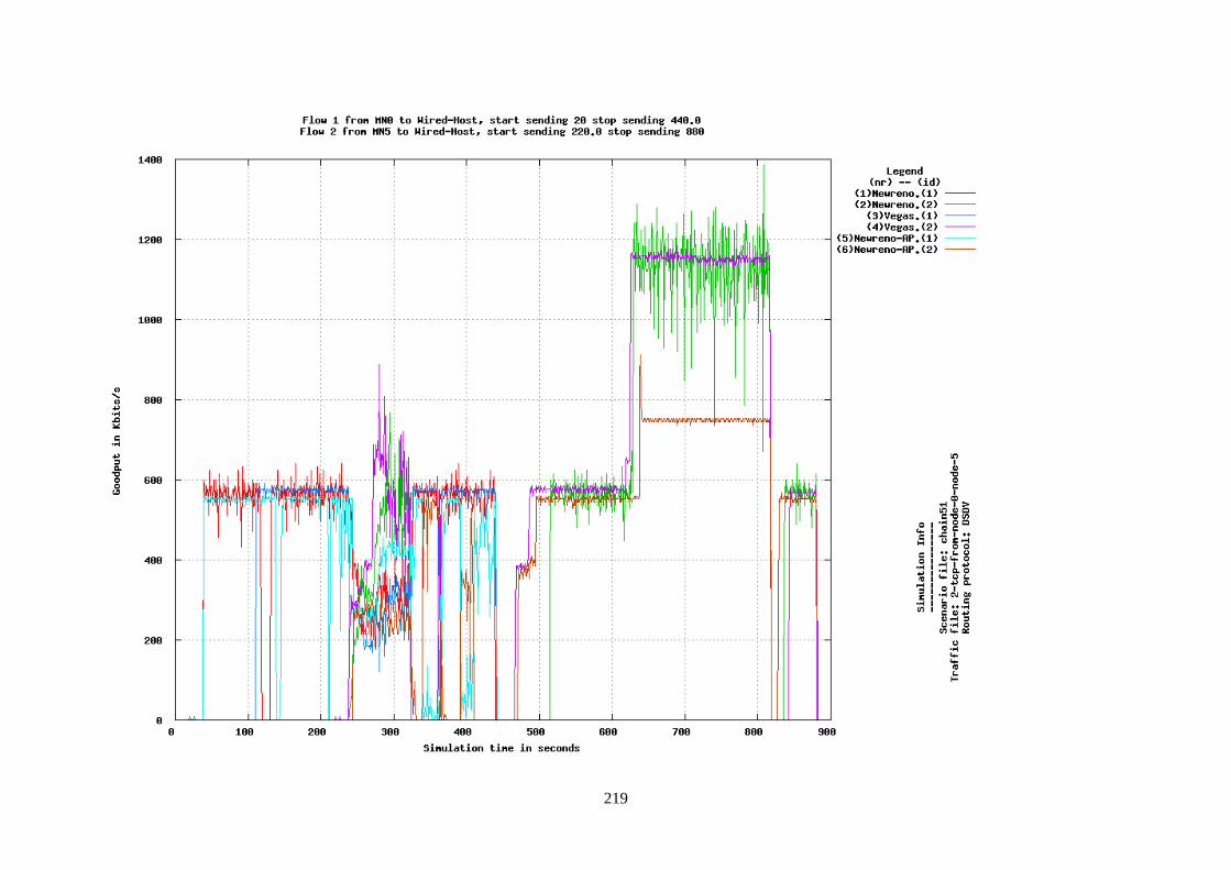
219
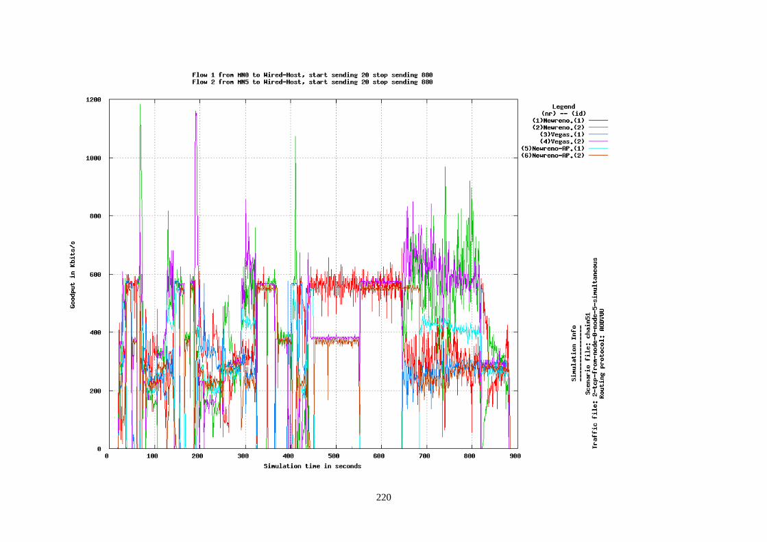
220
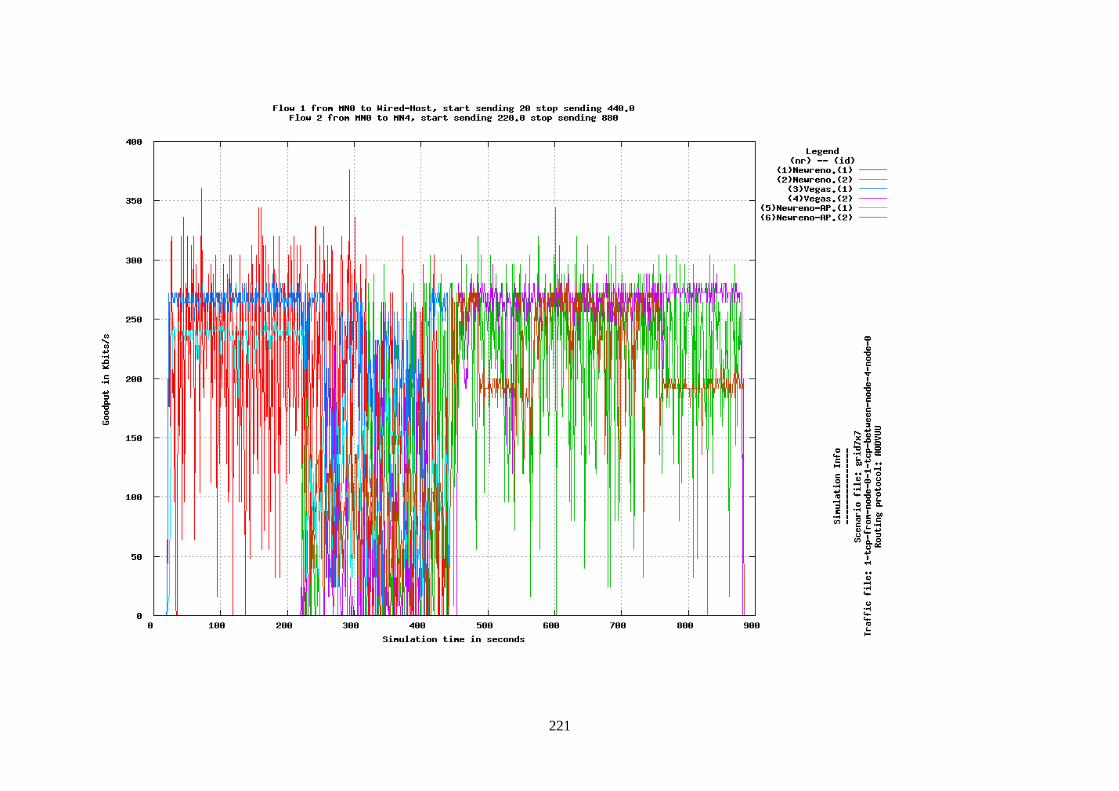
221
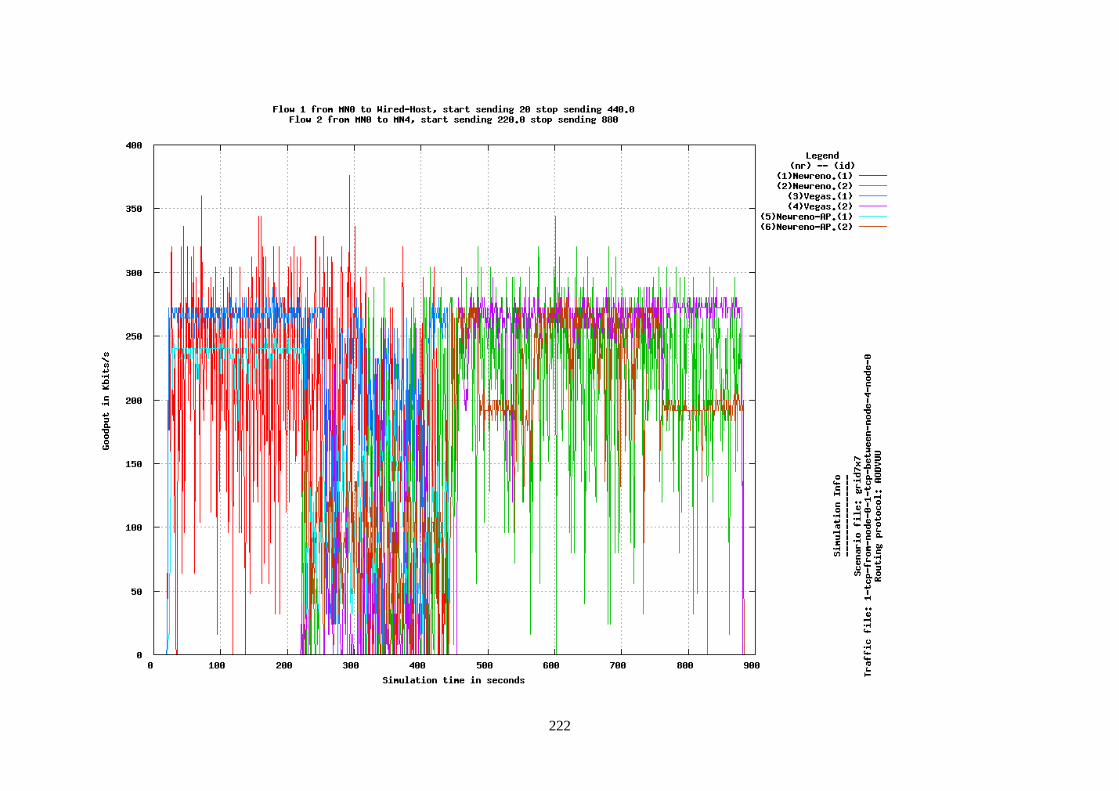
222
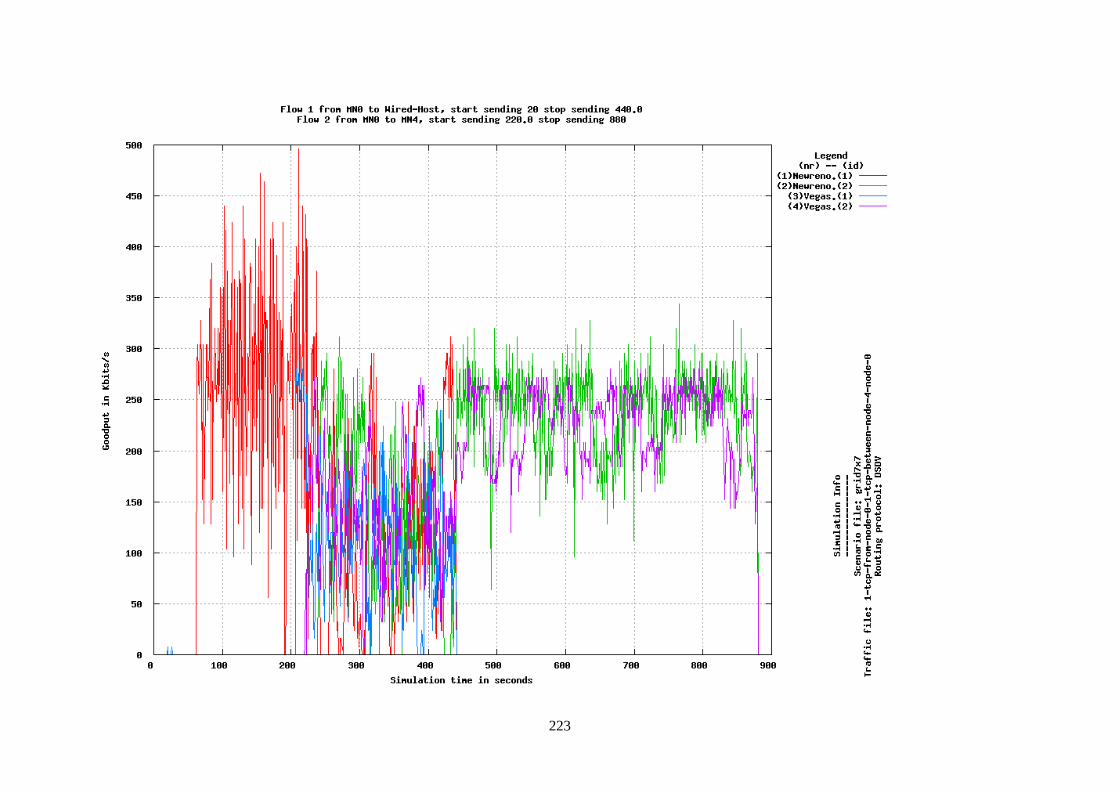
223
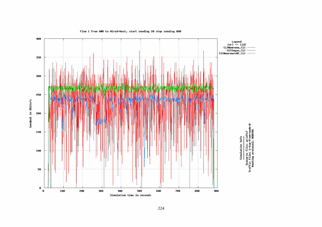
224

225
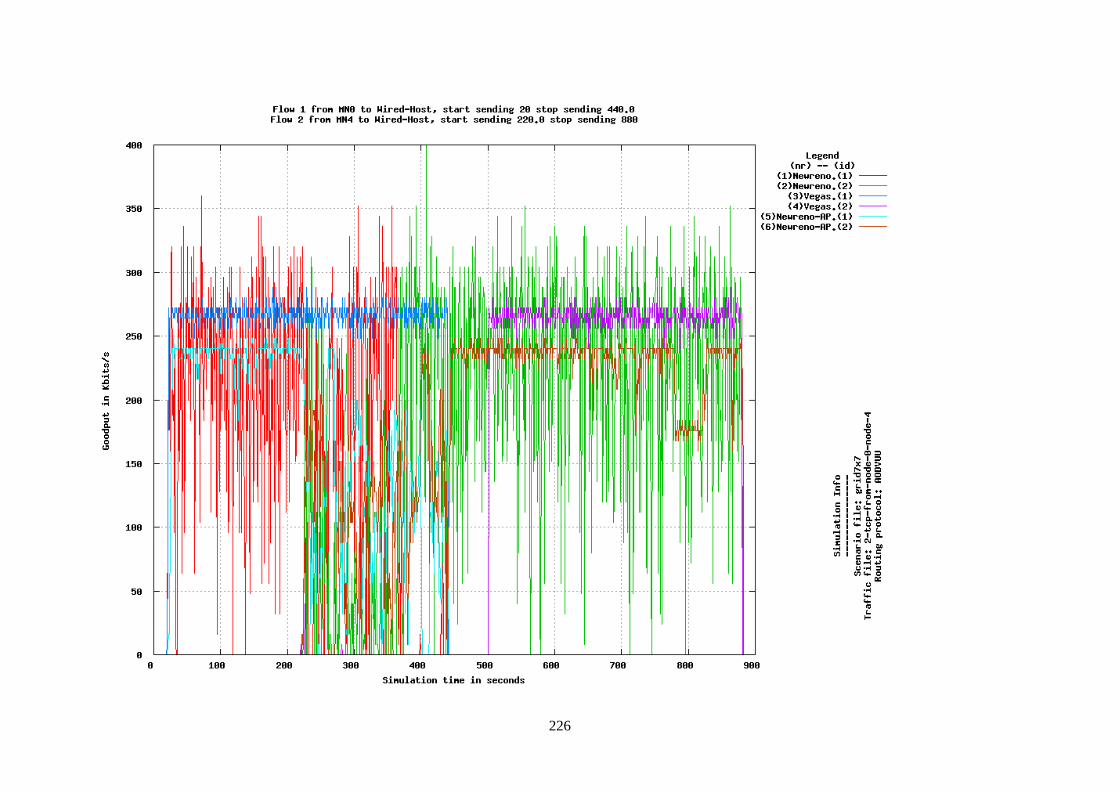
226
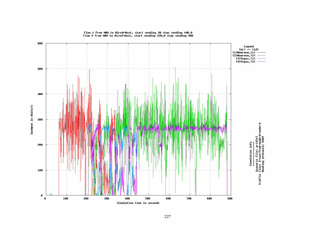
227
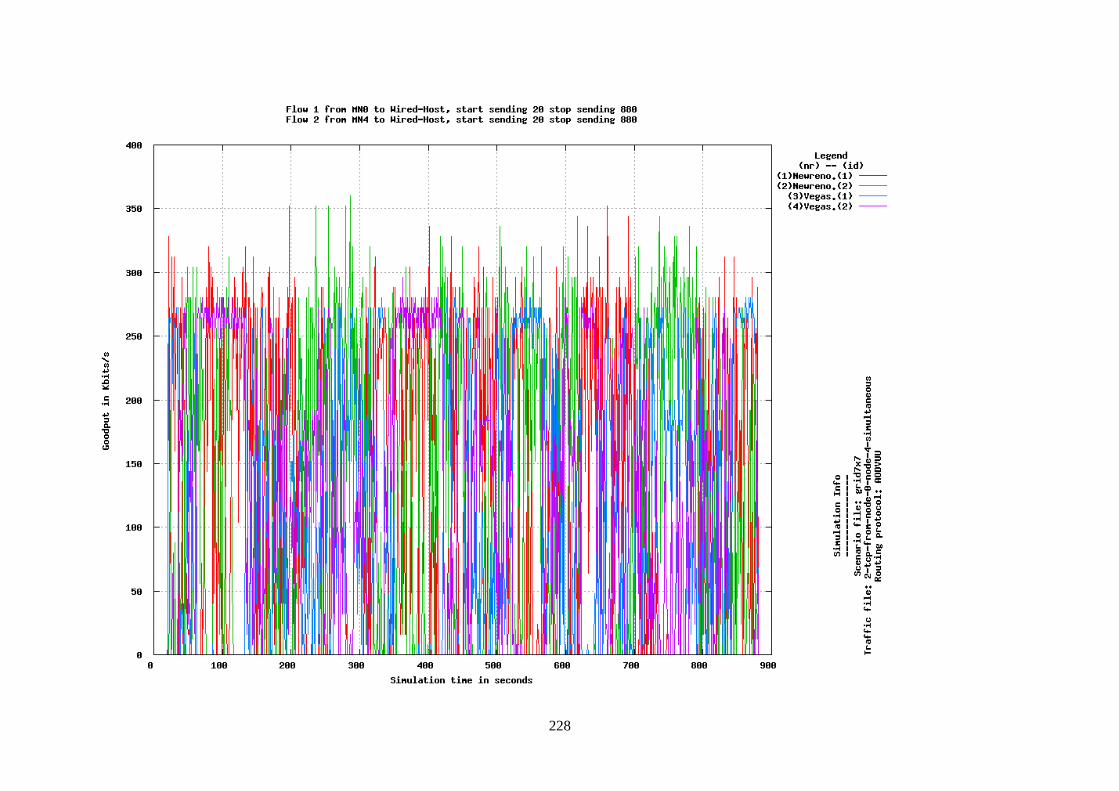
228

229
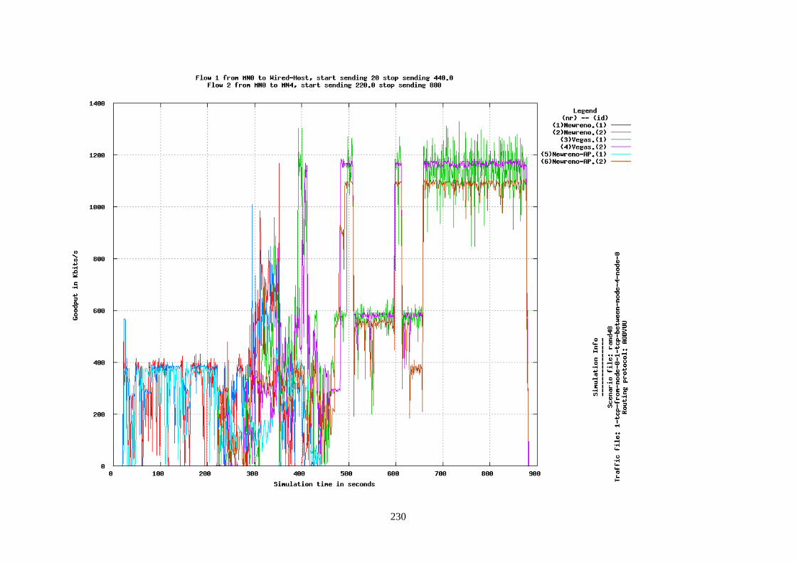
230
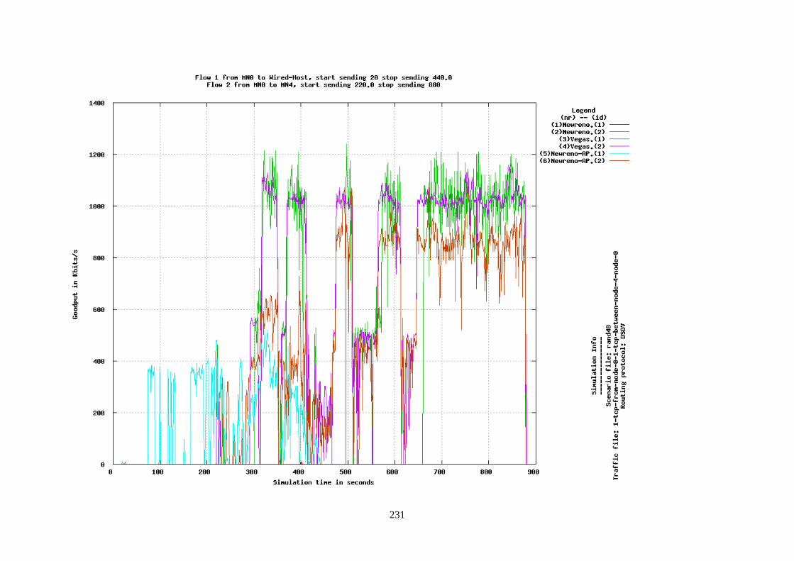
231
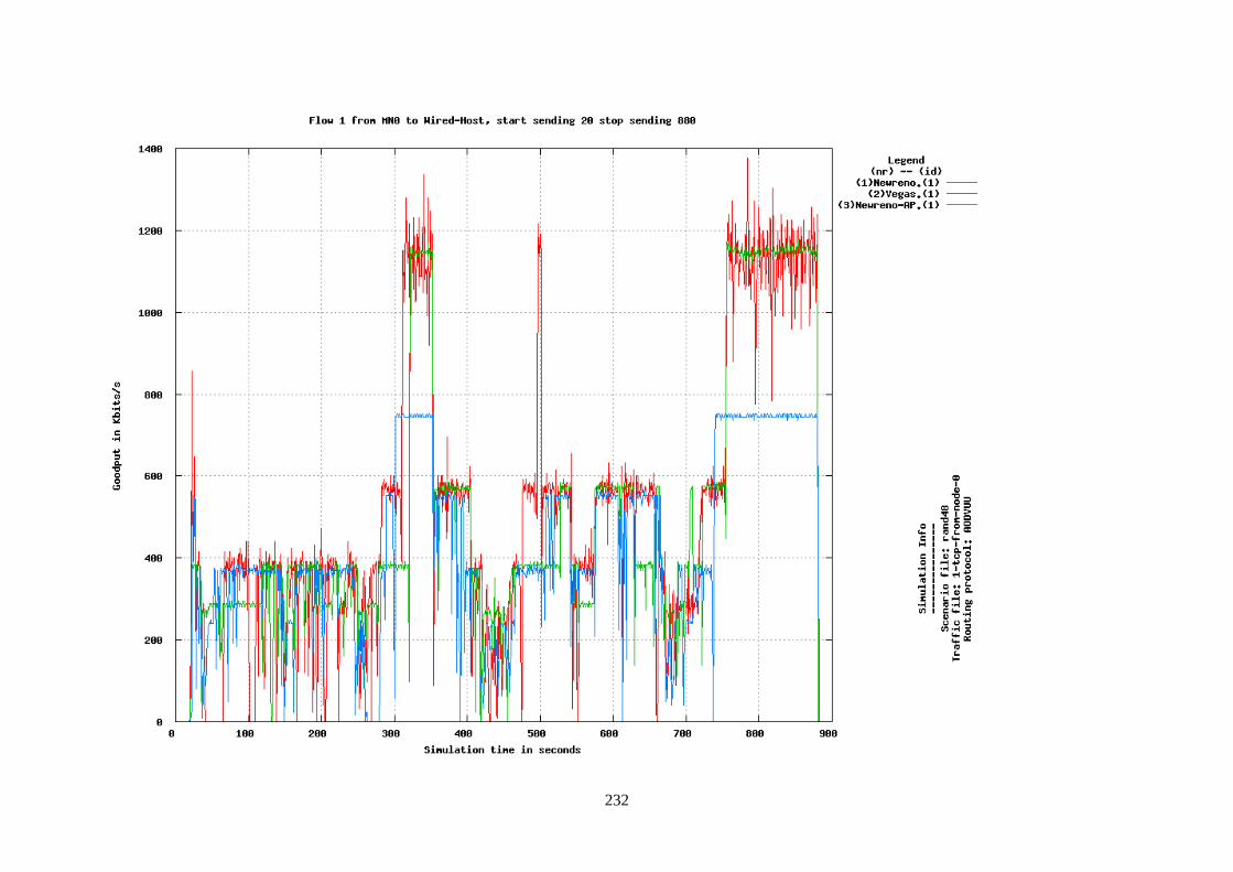
232
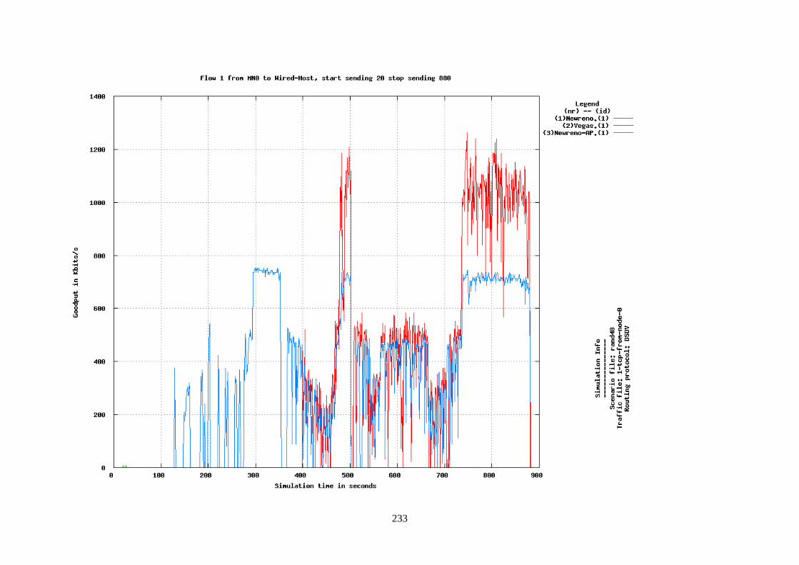
233
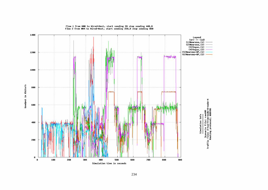
234
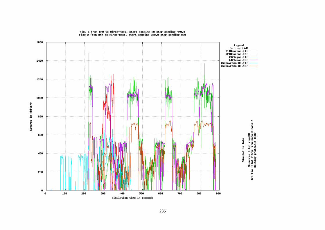
235
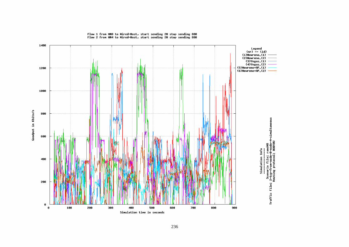
236
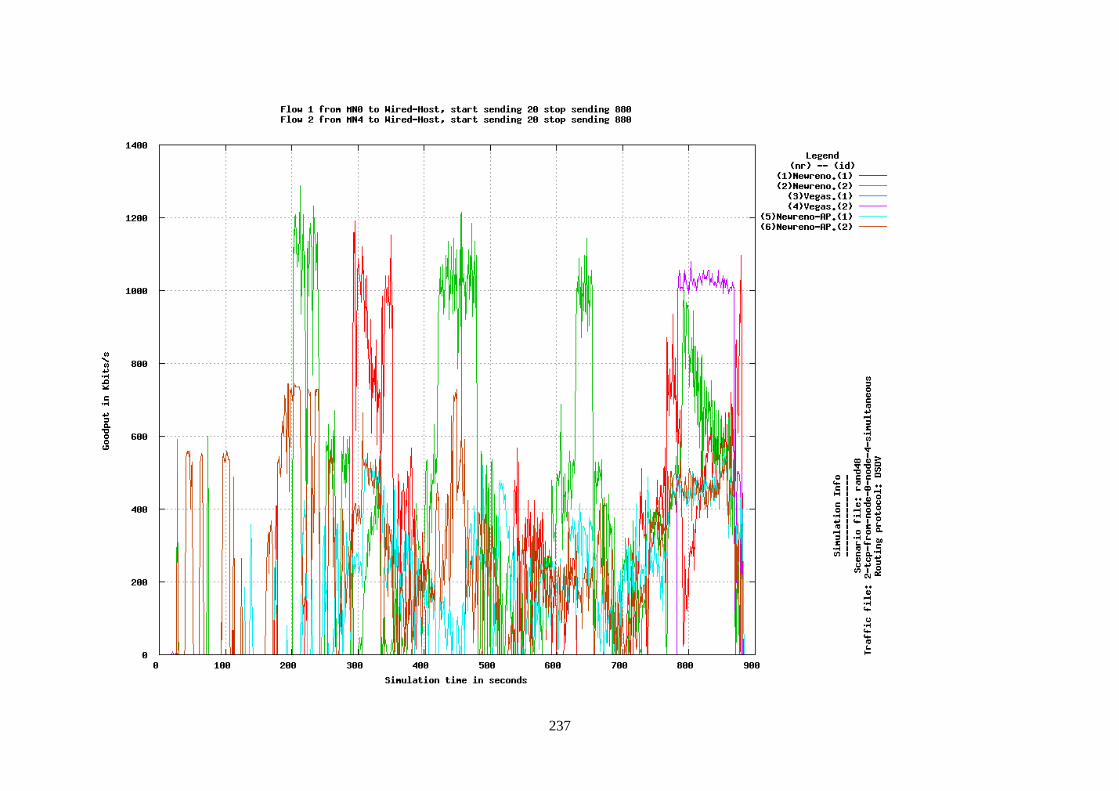
237
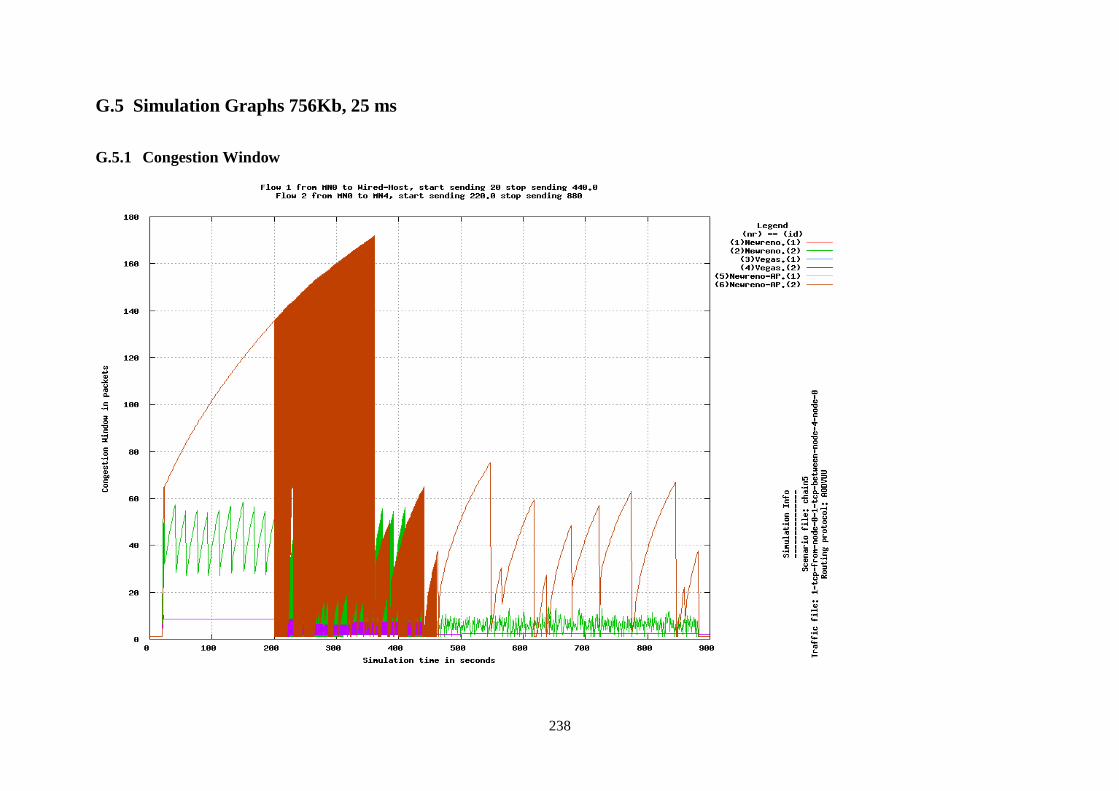
238
G.5 Simulation Graphs 756Kb, 25 ms
G.5.1 Congestion Window
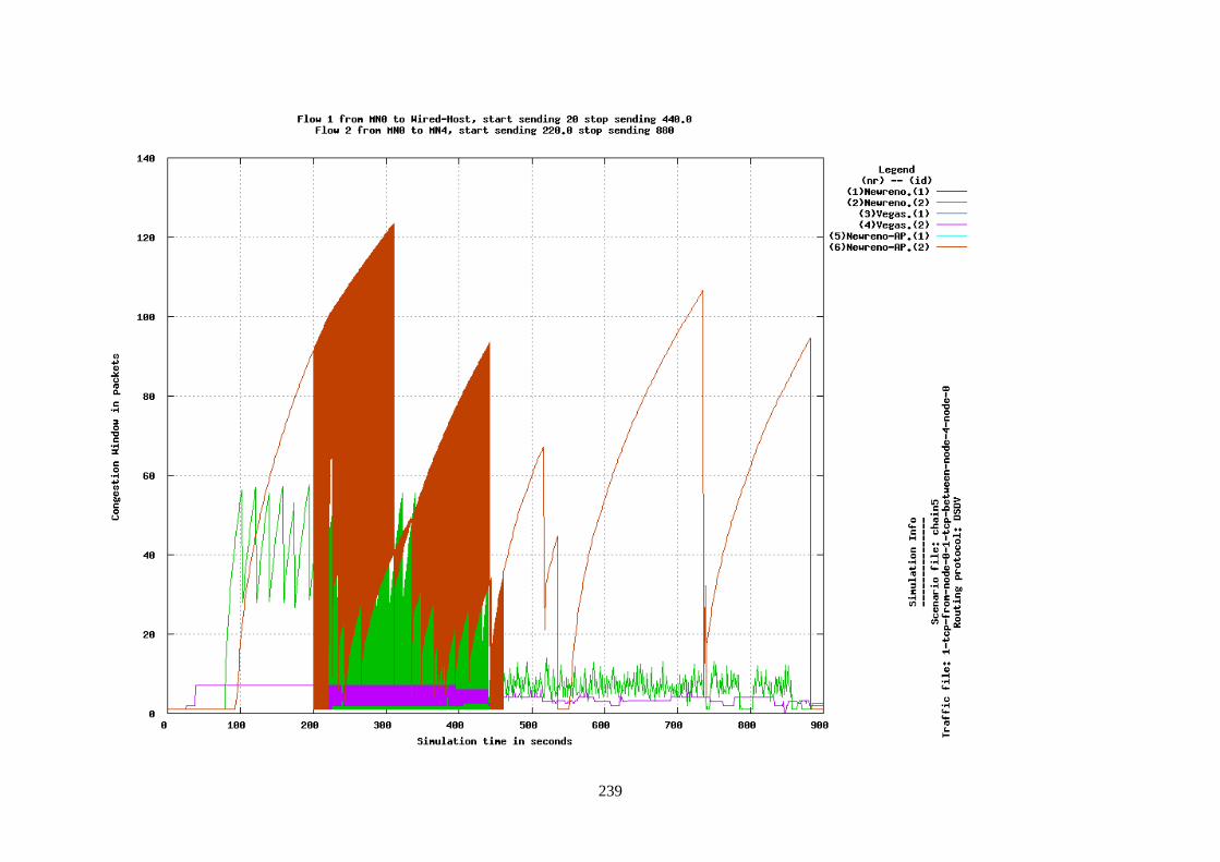
239
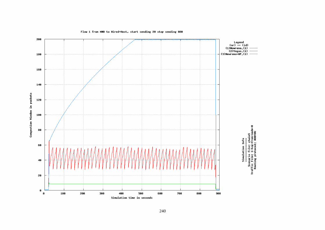
240

241
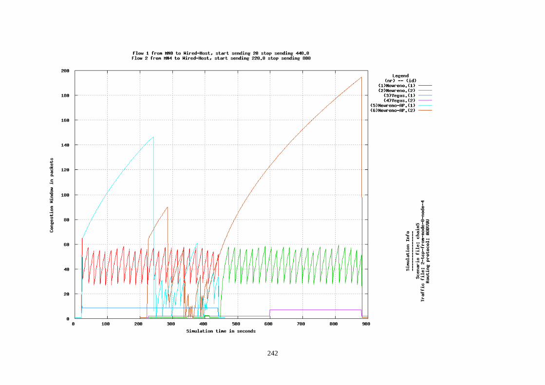
242
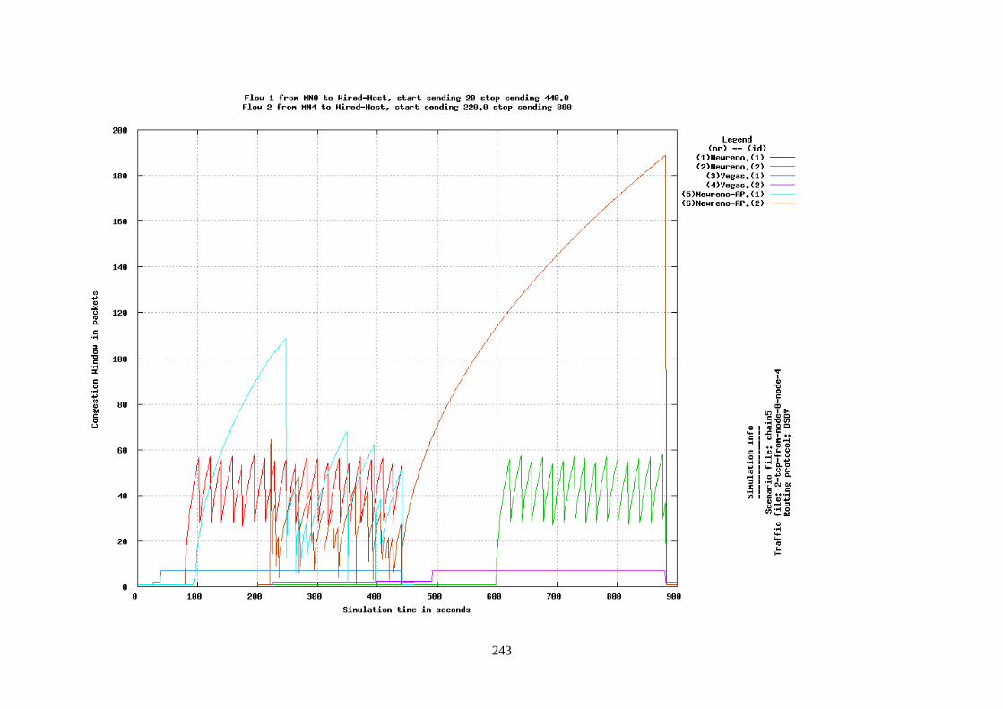
243
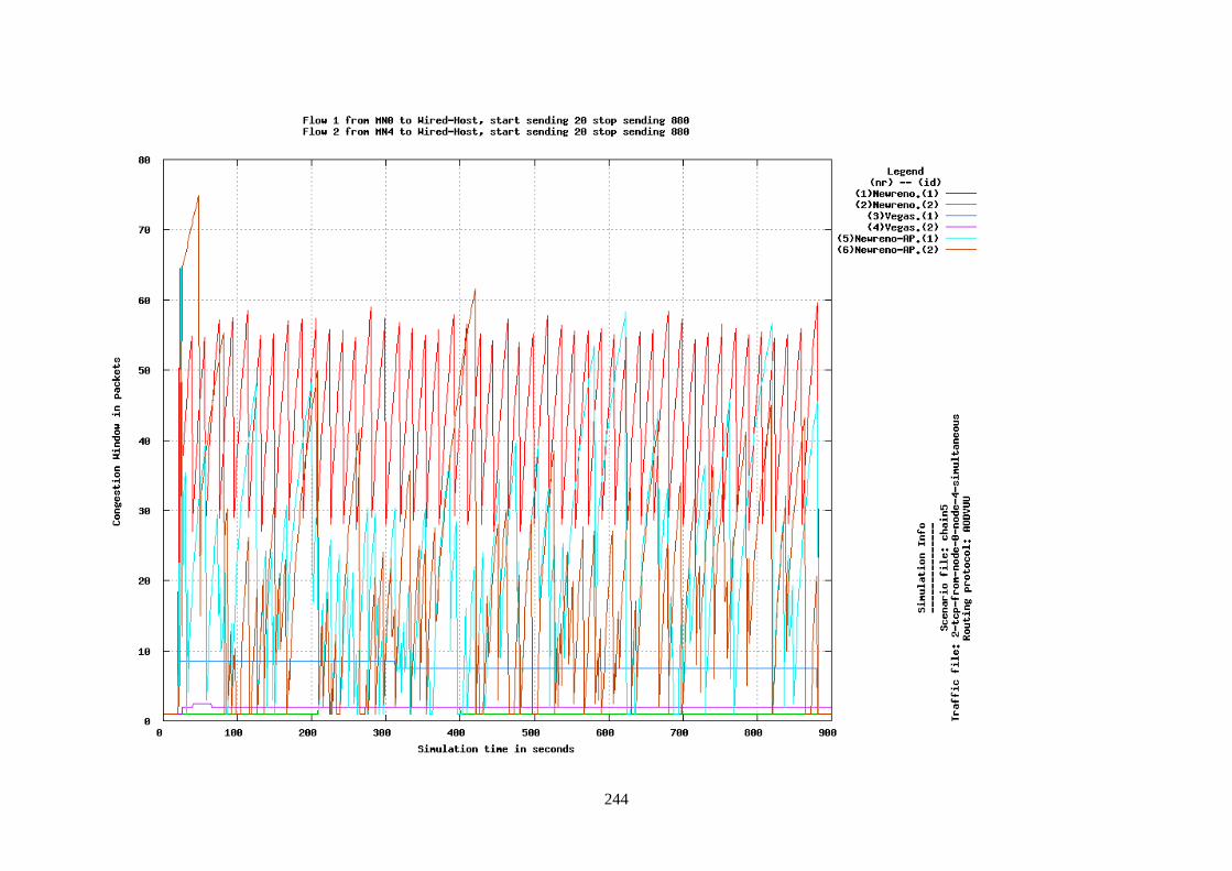
244

245
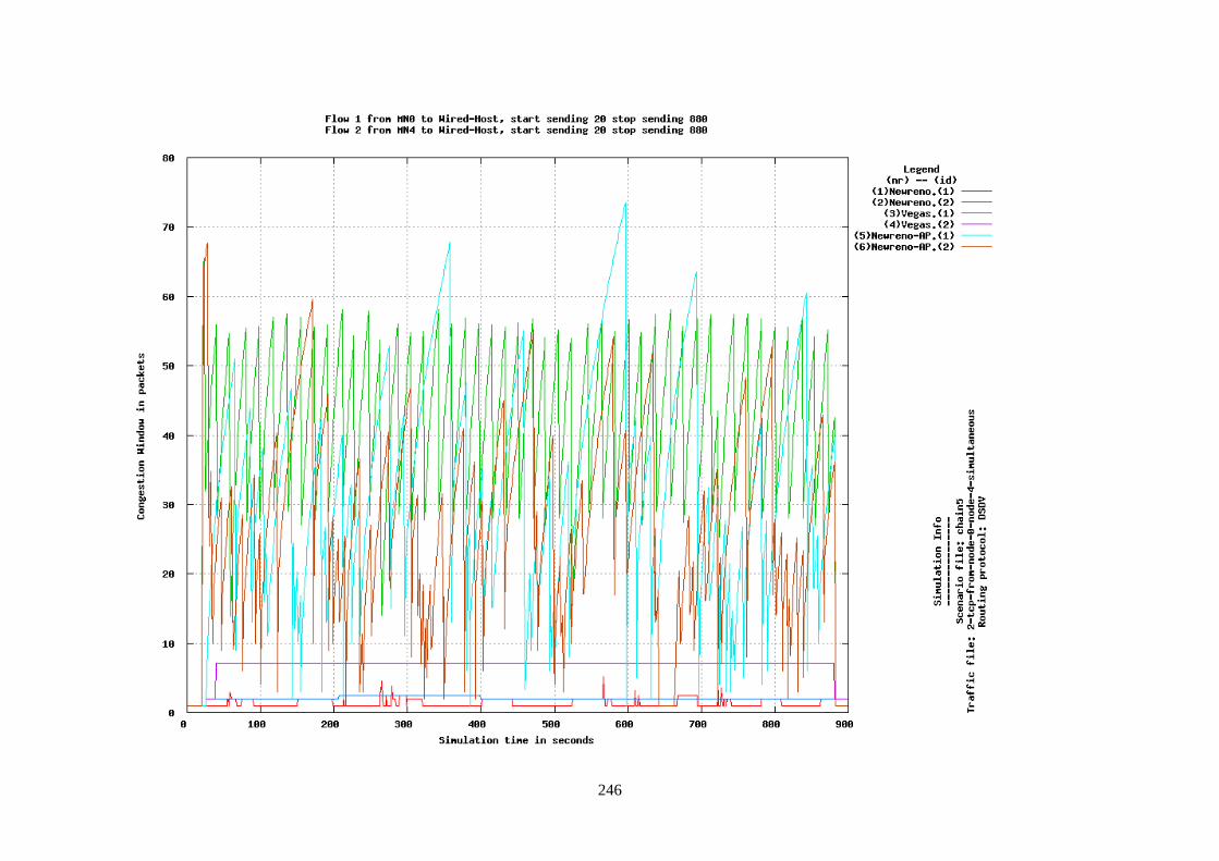
246
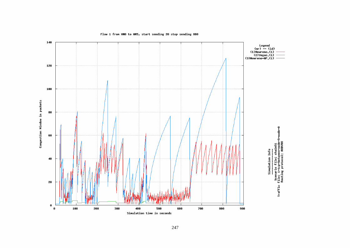
247
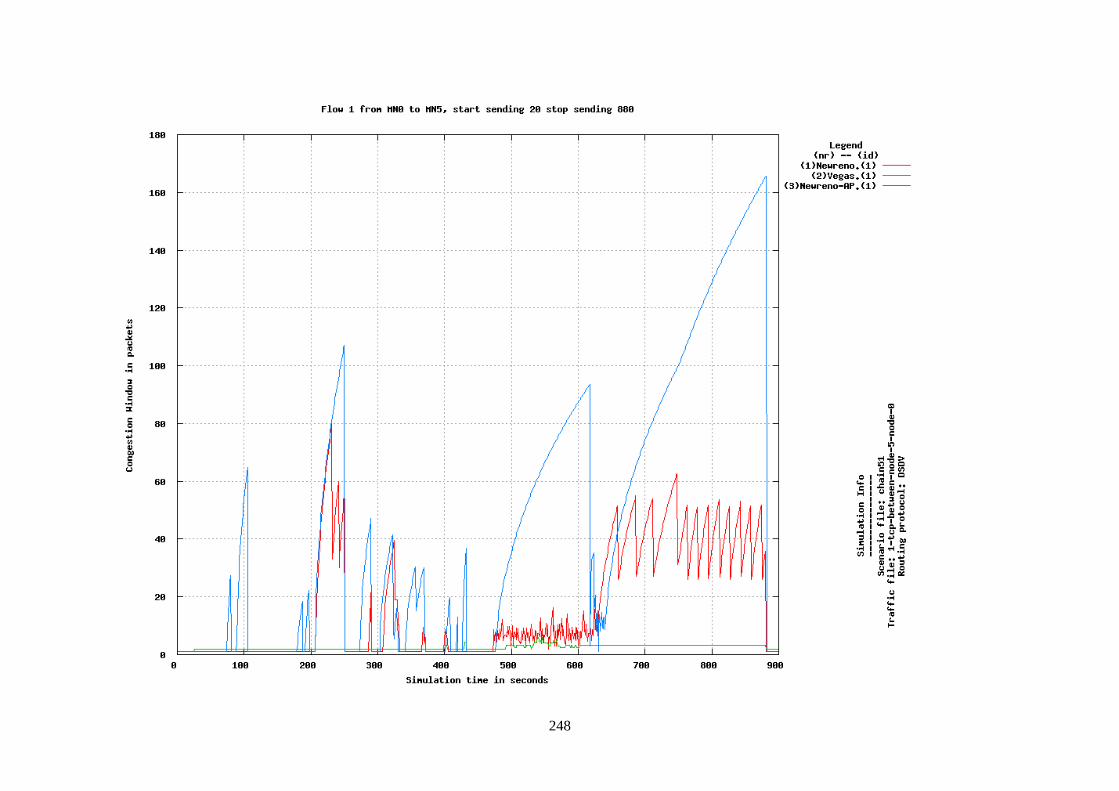
248
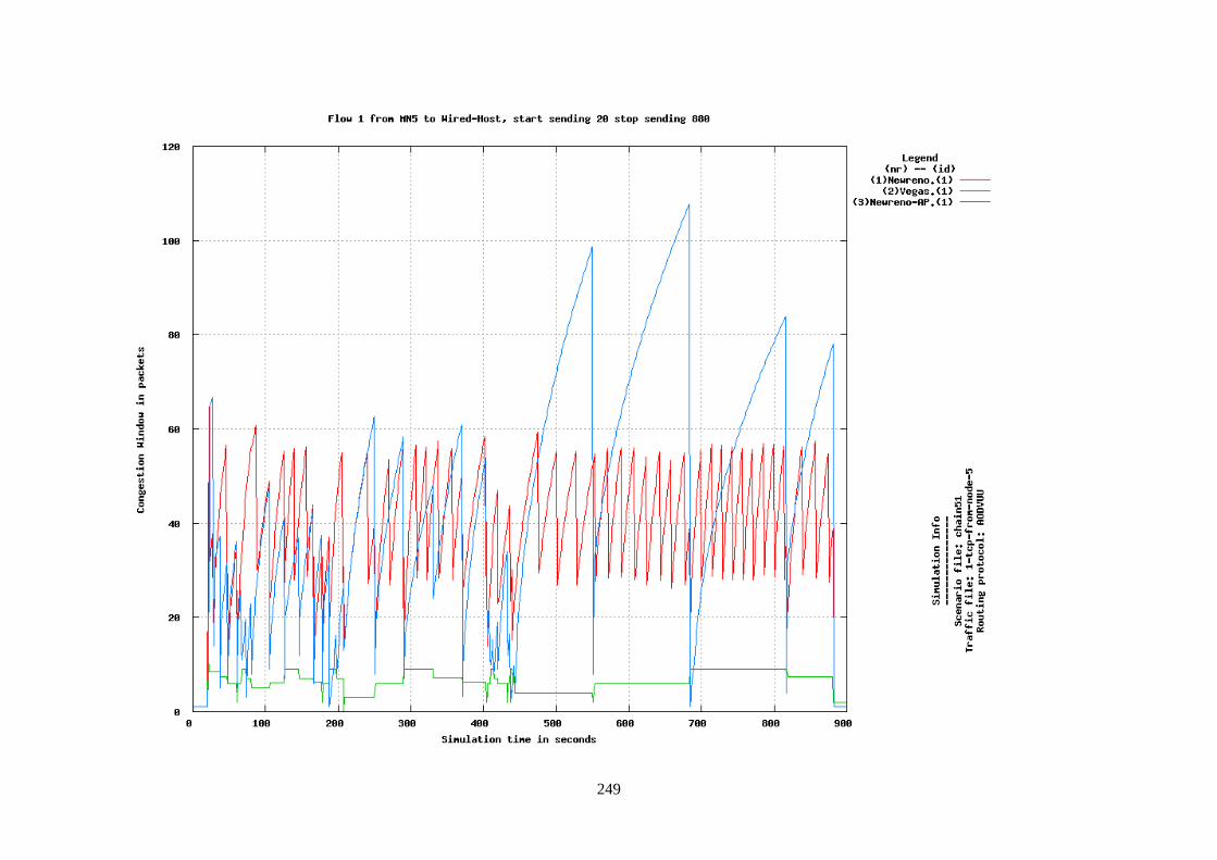
249
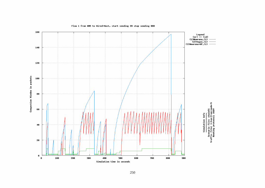
250
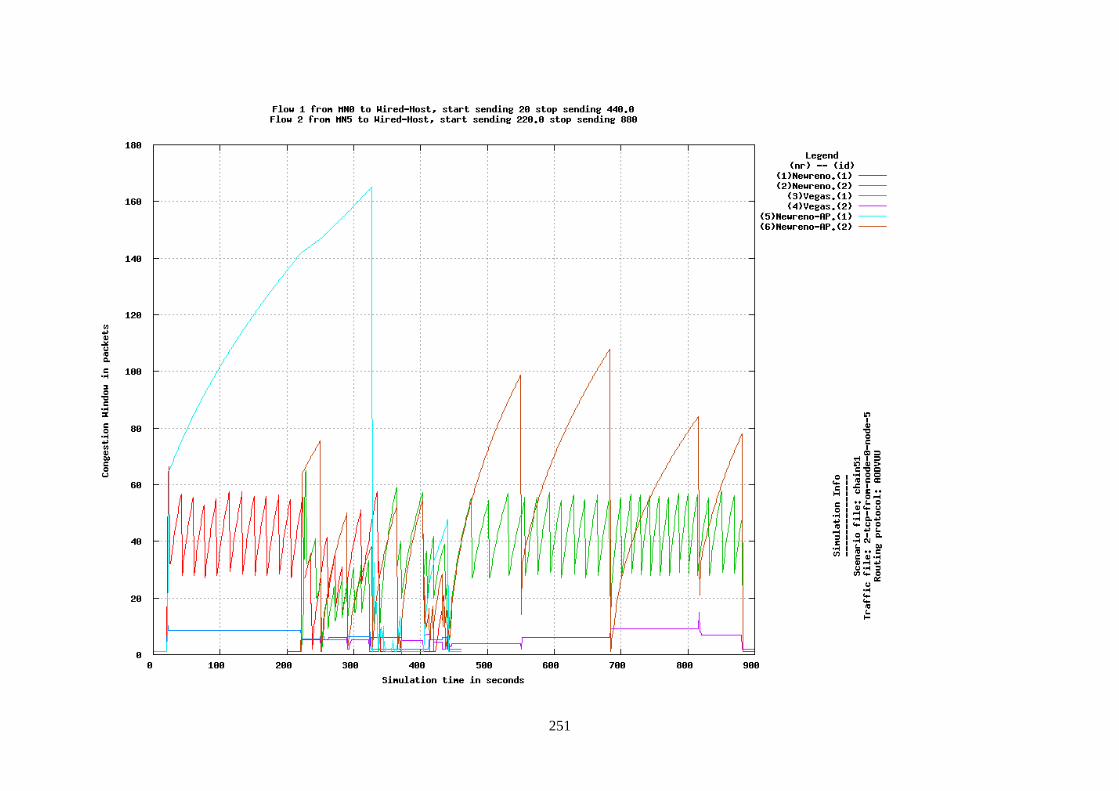
251
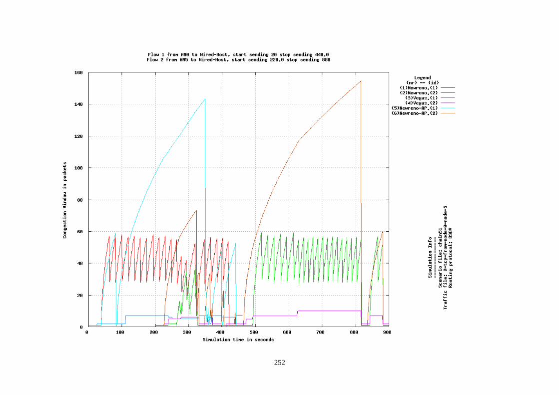
252
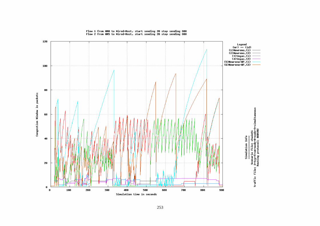
253
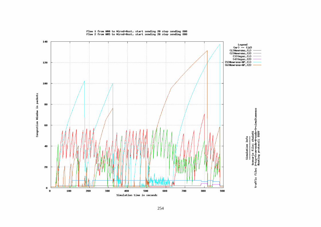
254
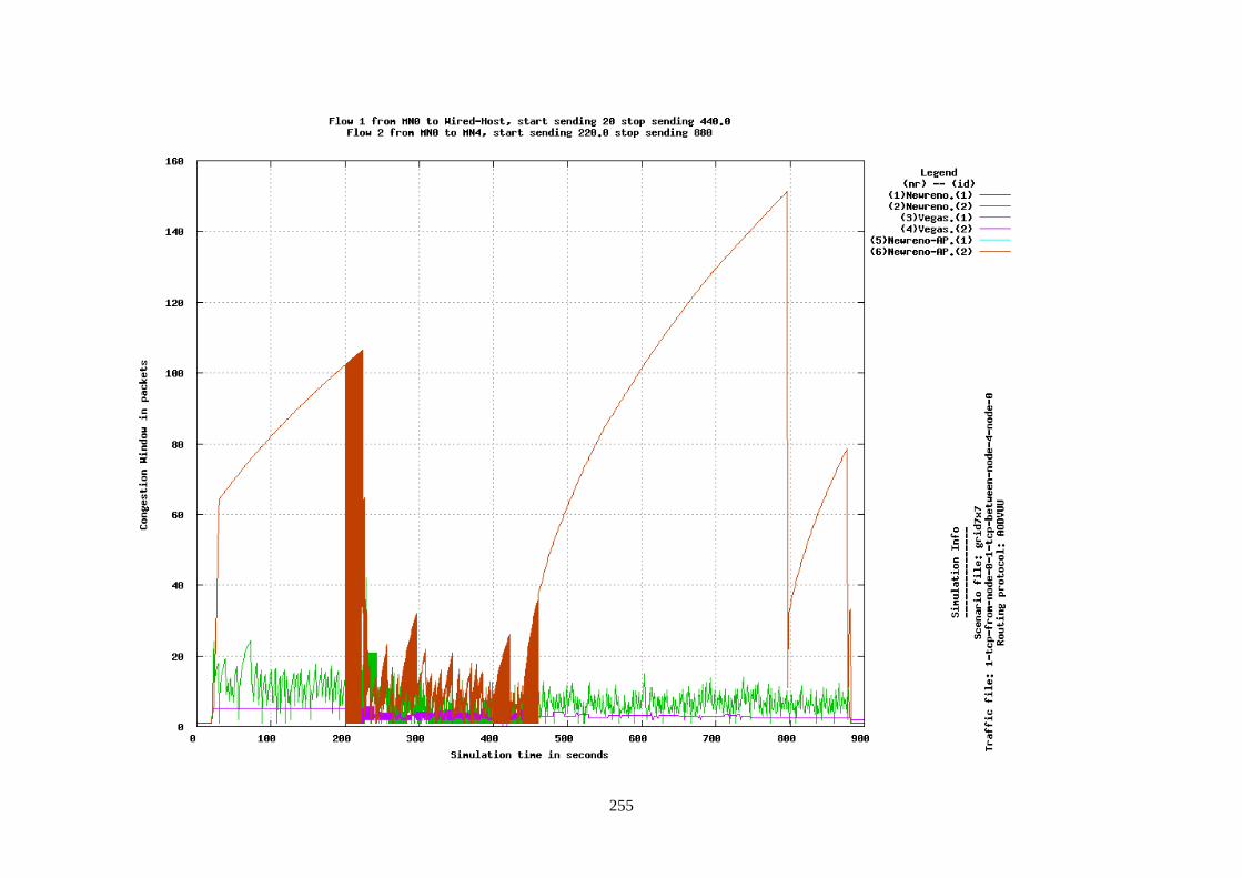
255
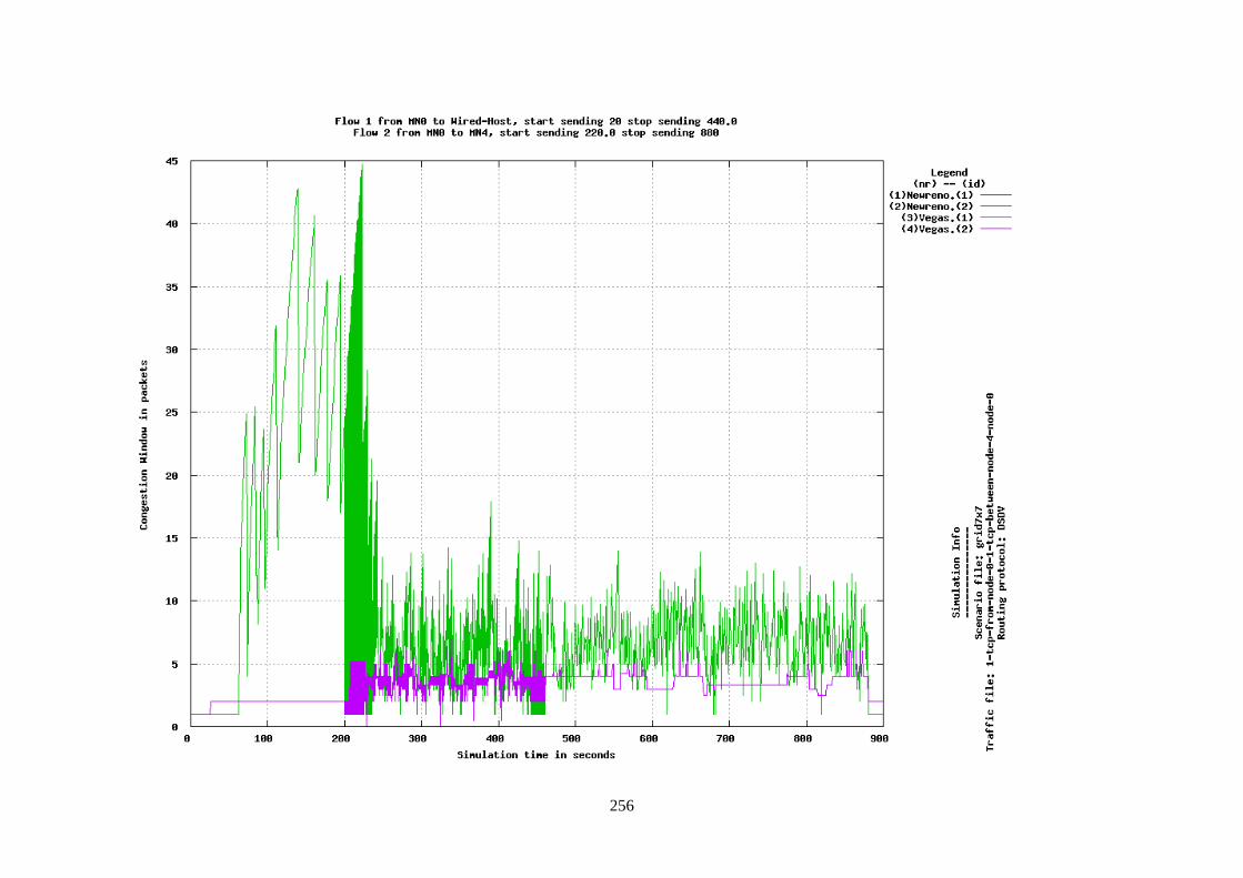
256
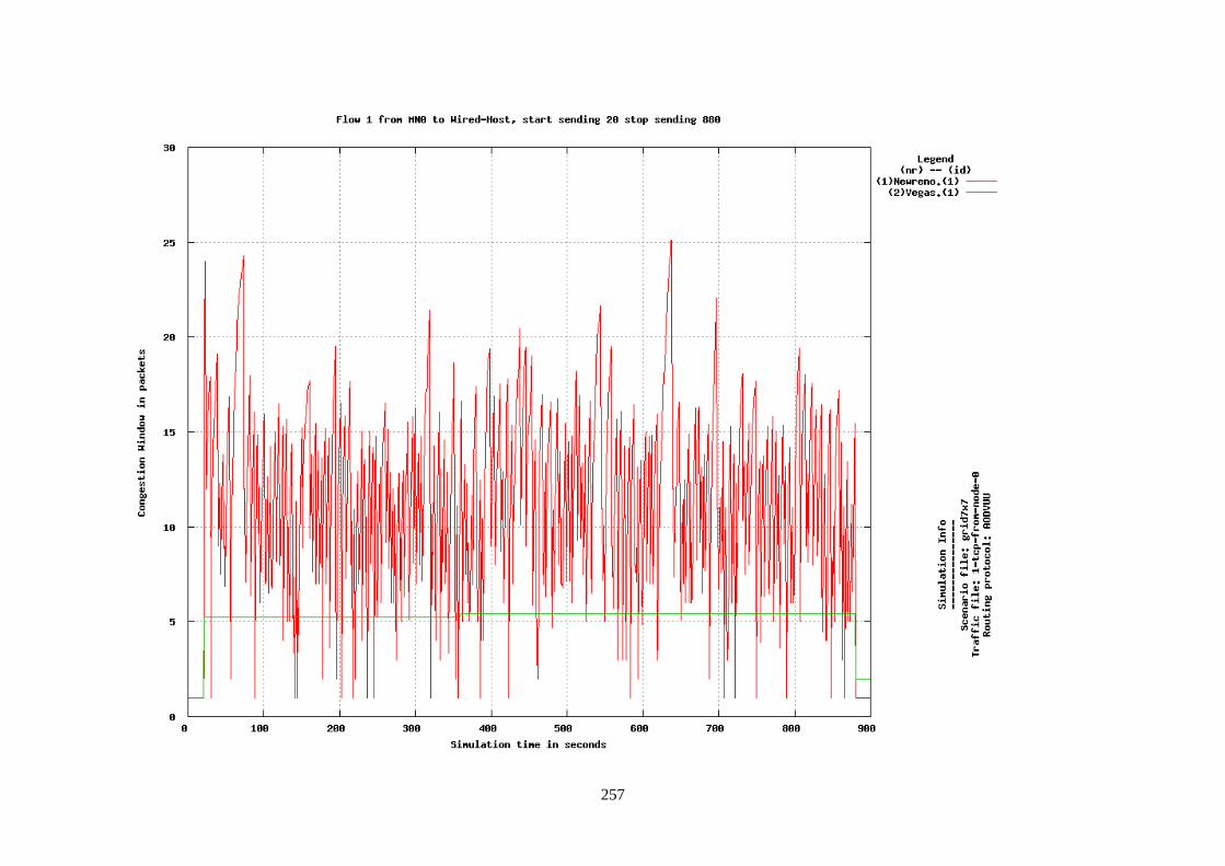
257
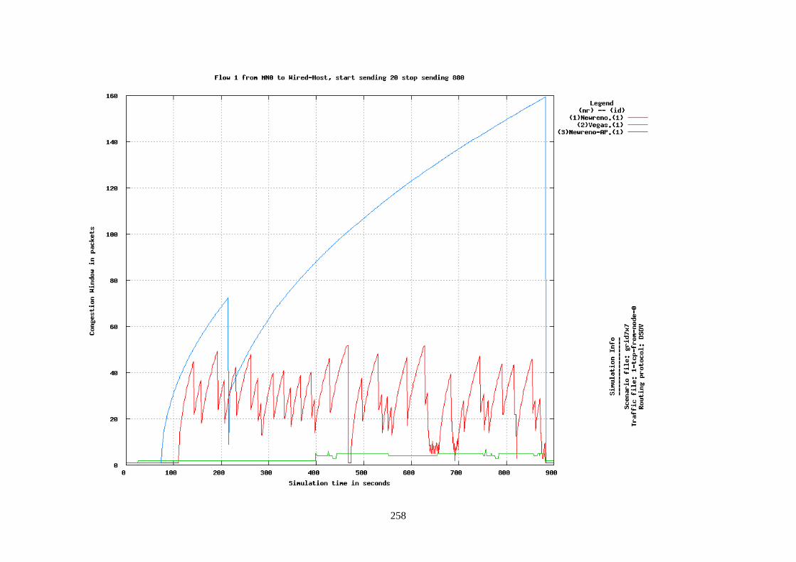
258
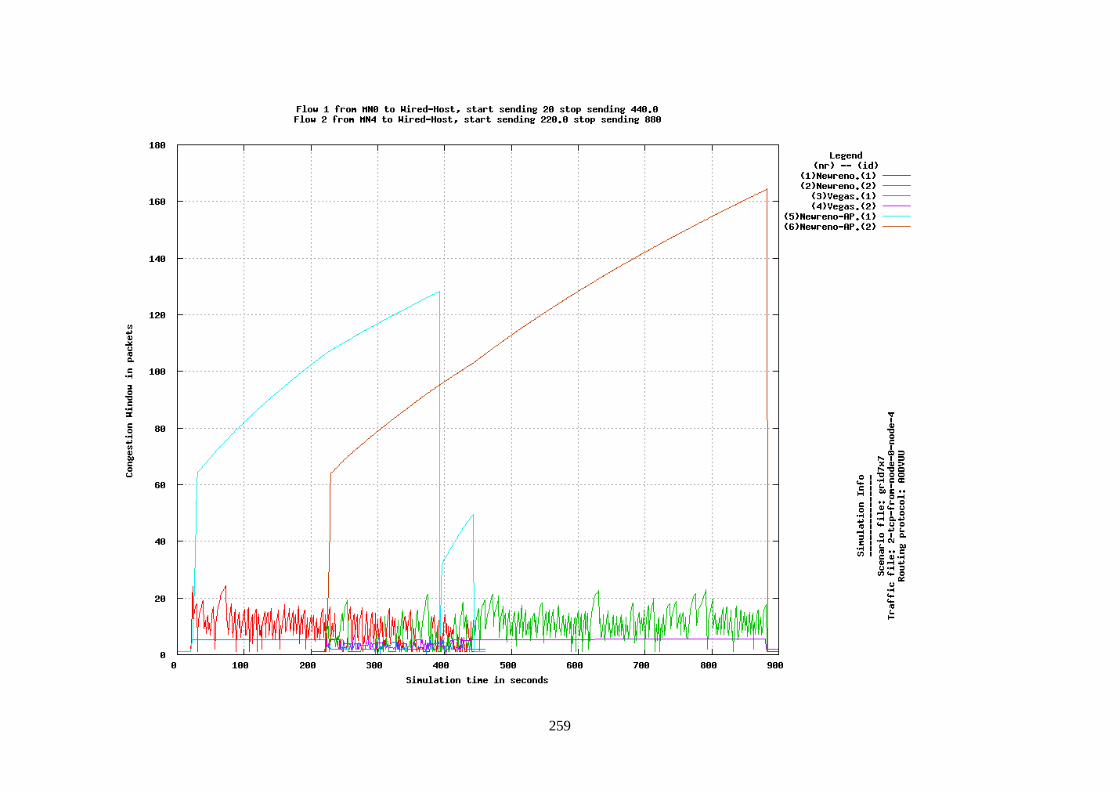
259
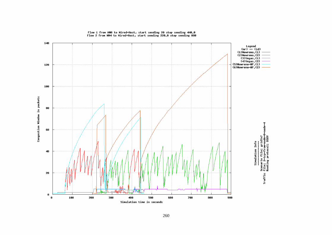
260
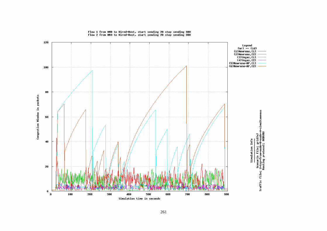
261
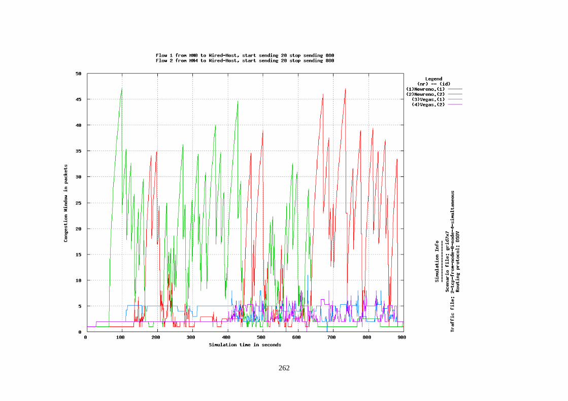
262
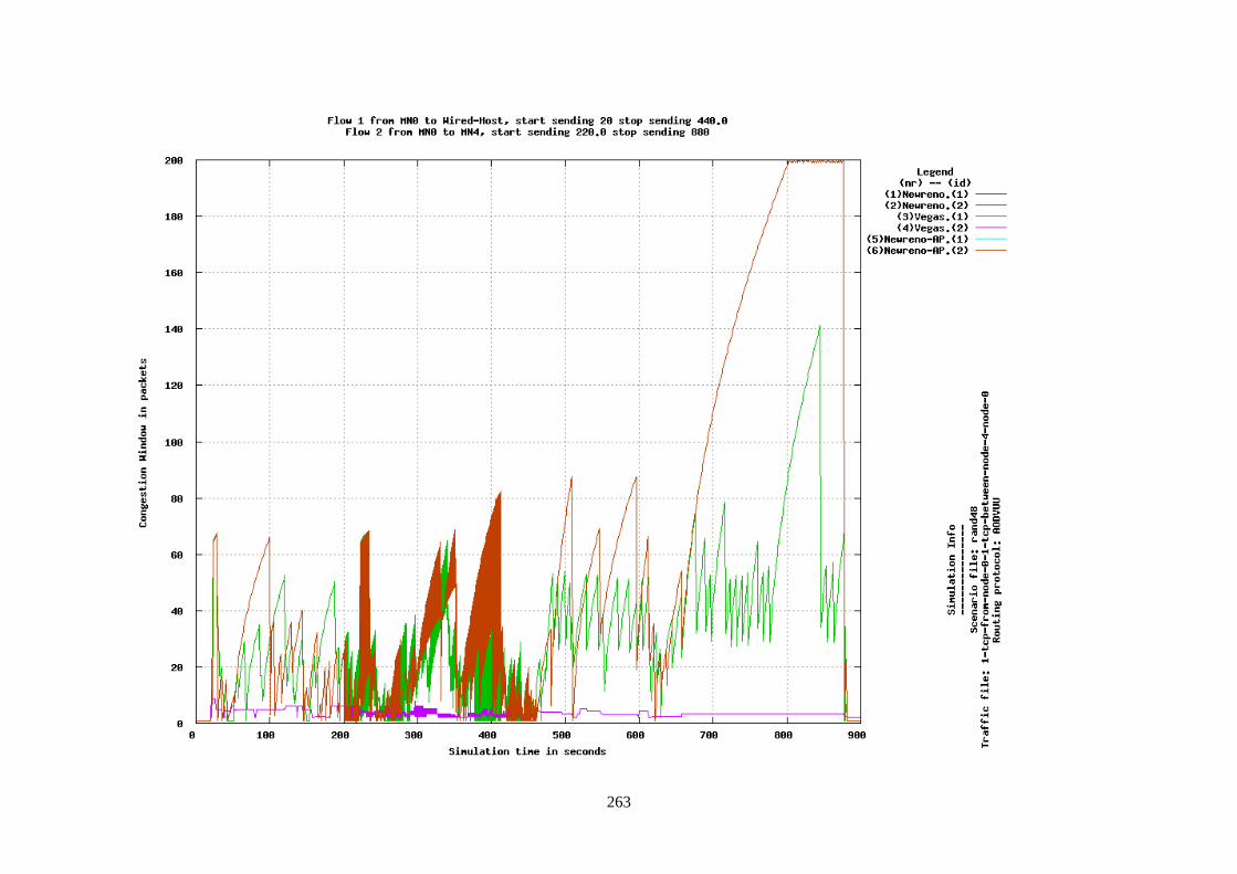
263
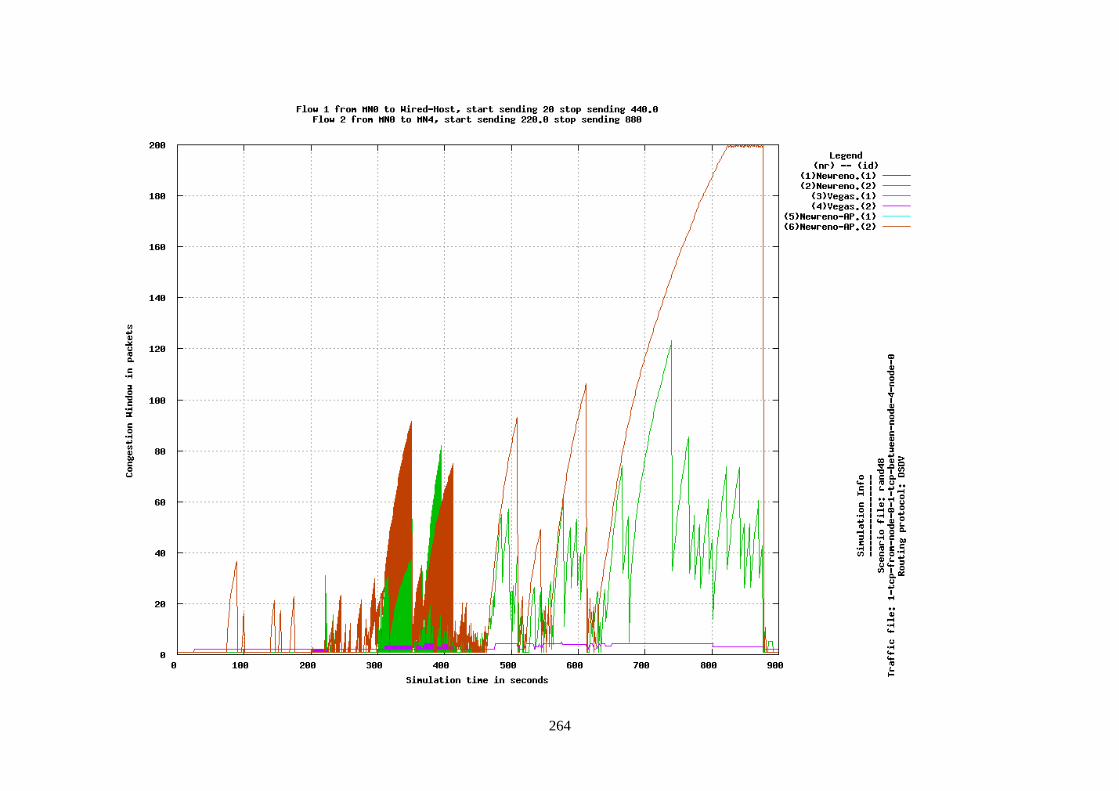
264
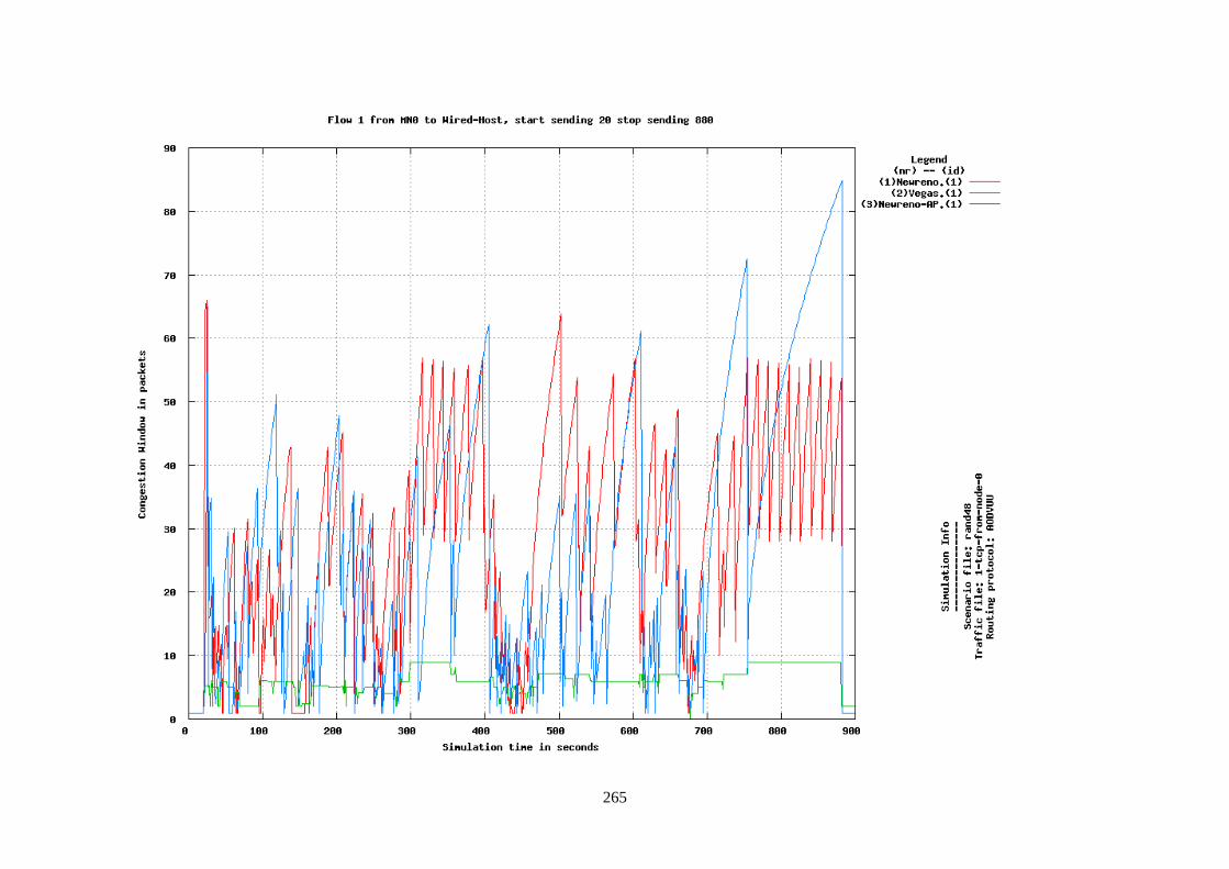
265
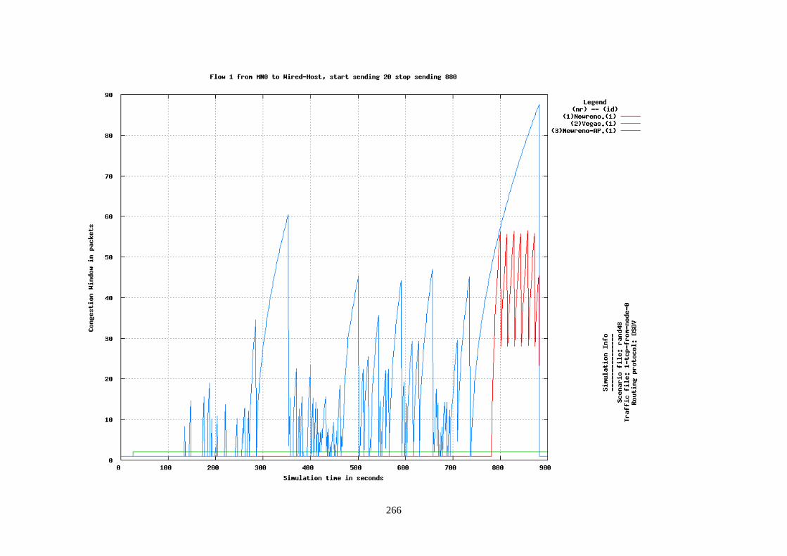
266
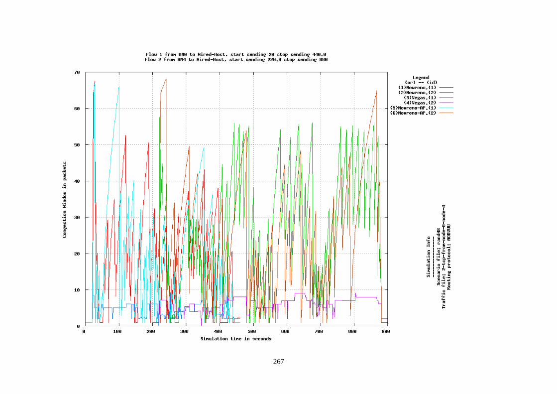
267
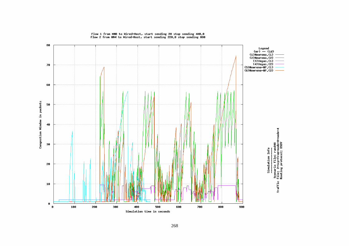
268
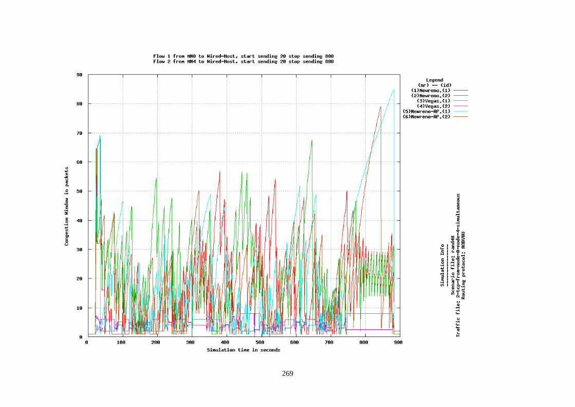
269
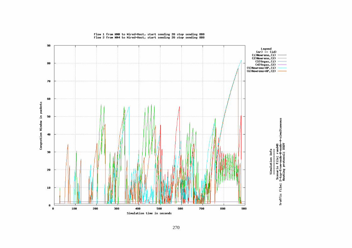
270
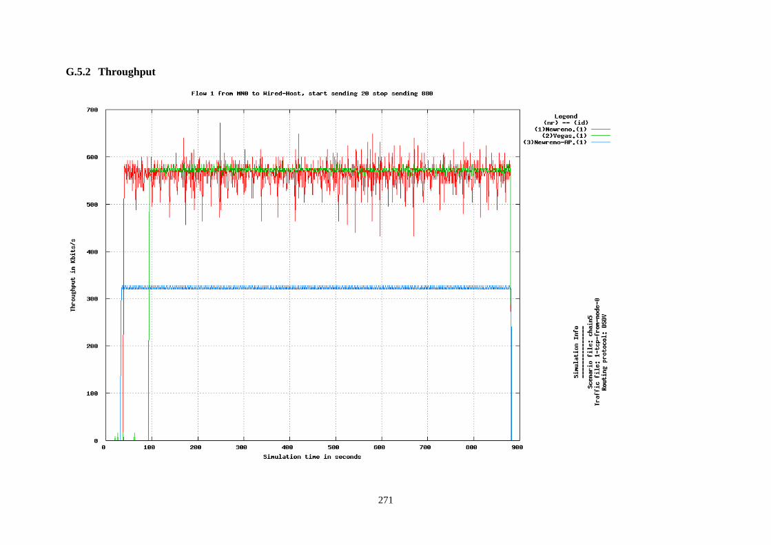
271
G.5.2 Throughput
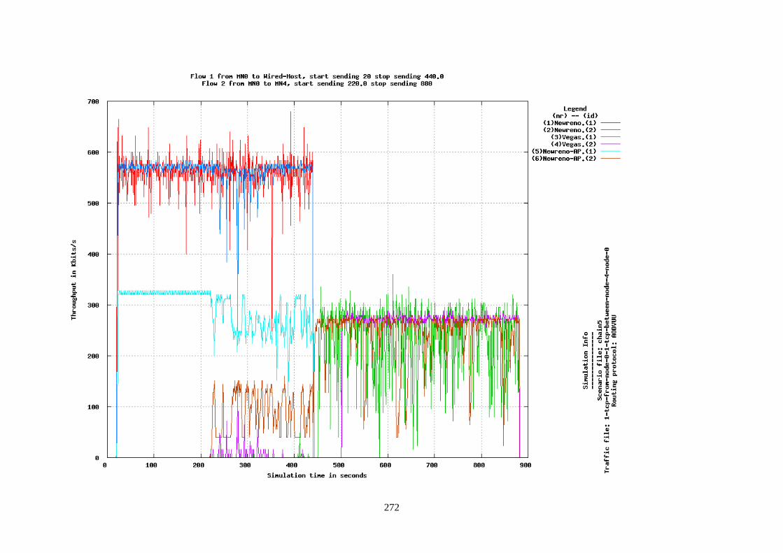
272
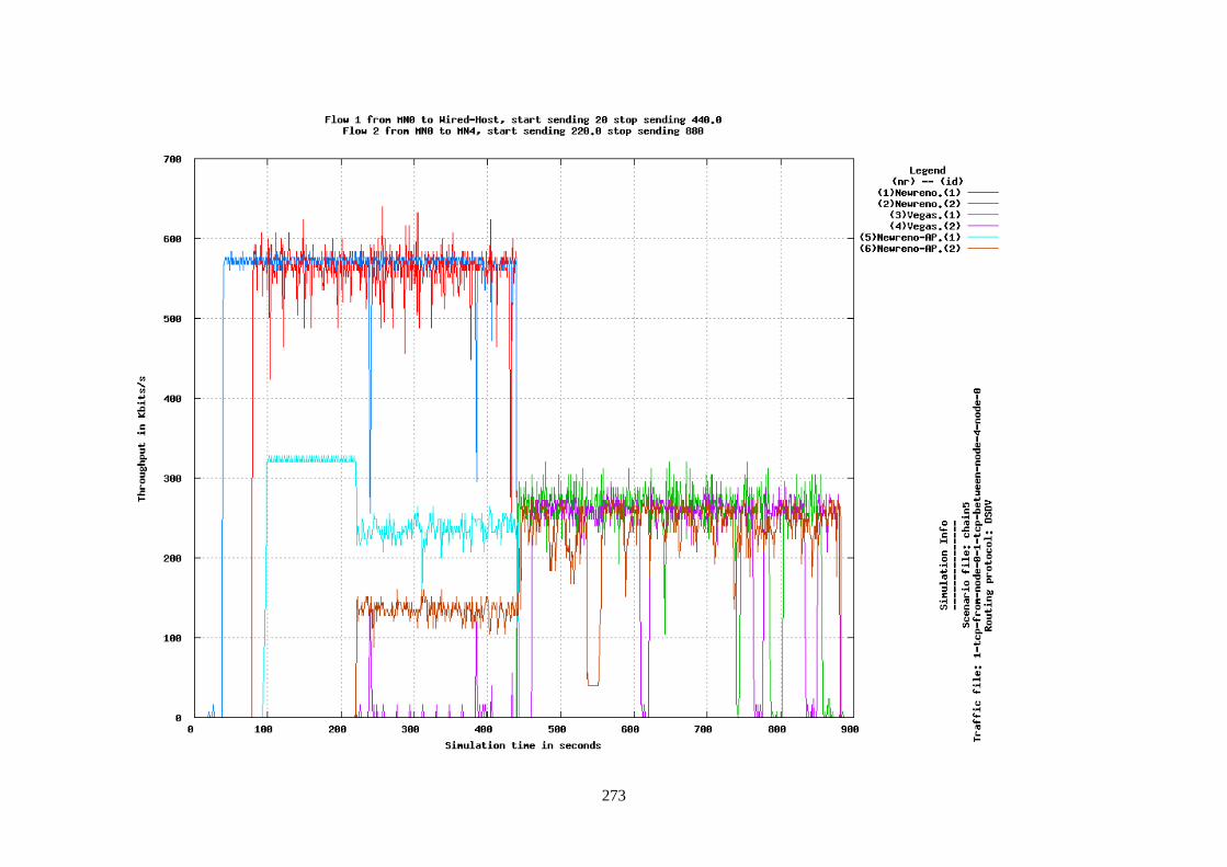
273
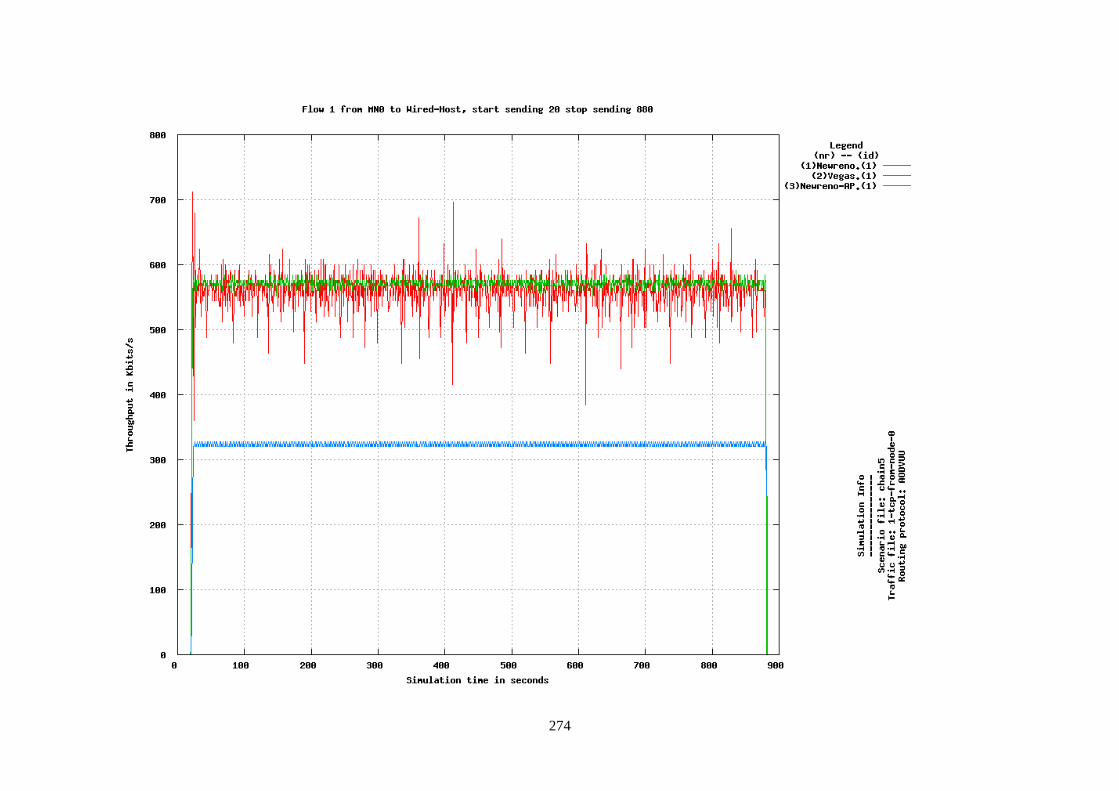
274
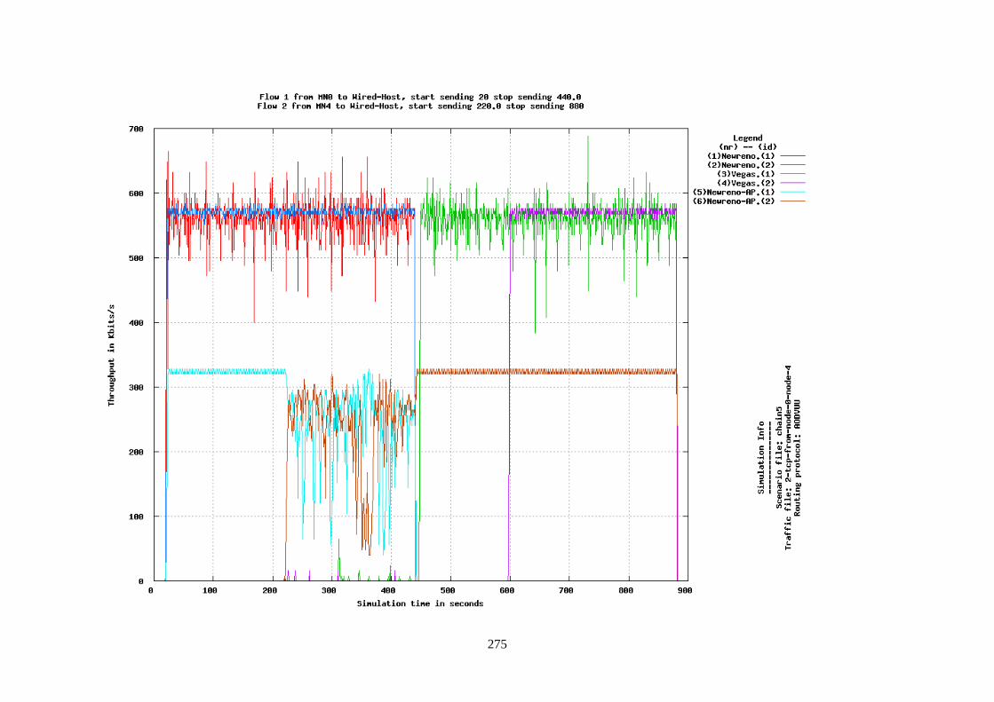
275
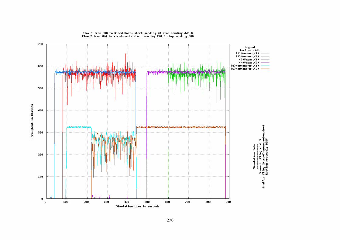
276
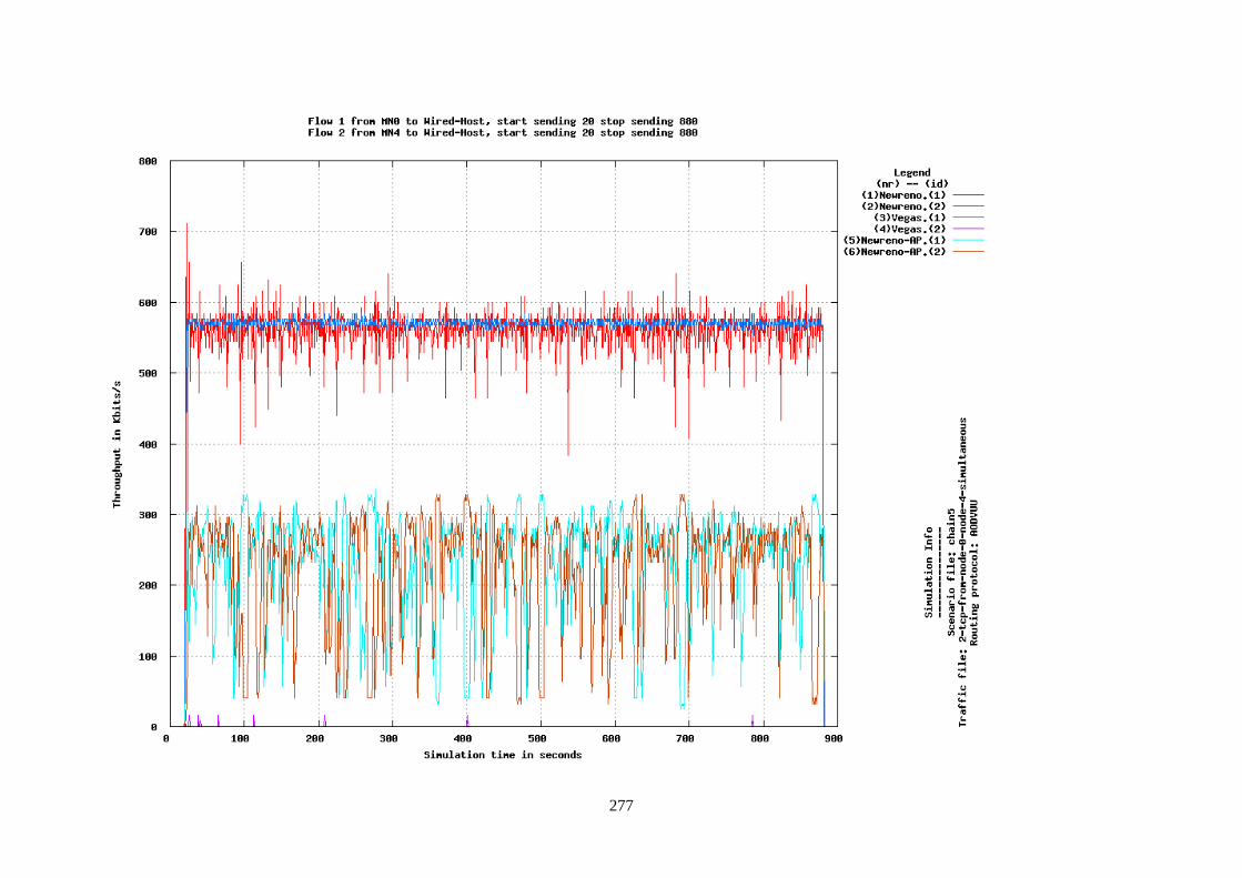
277
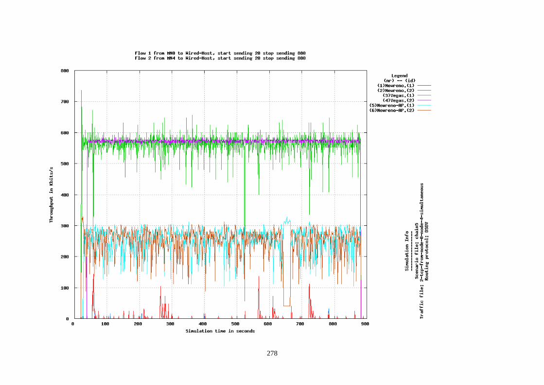
278
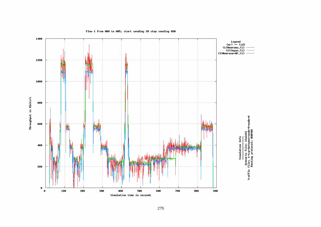
279
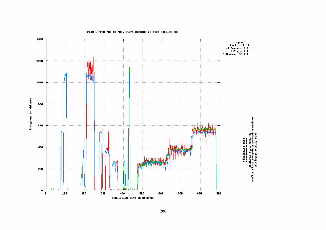
280
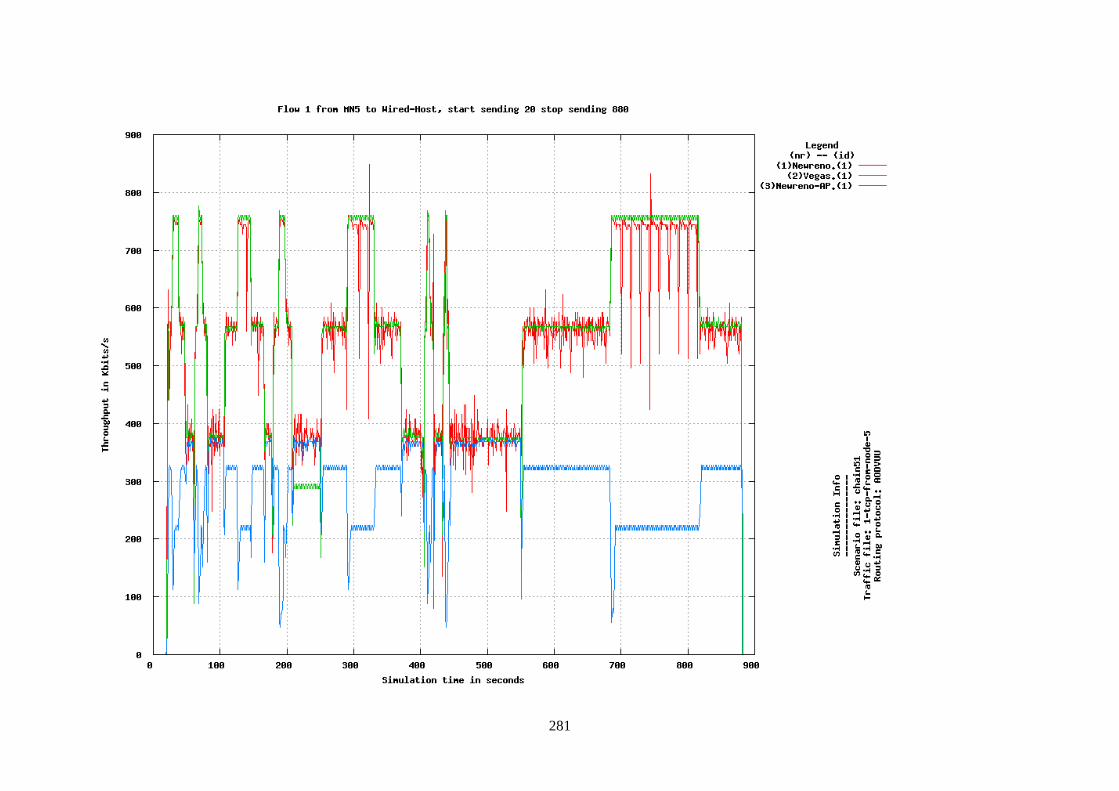
281
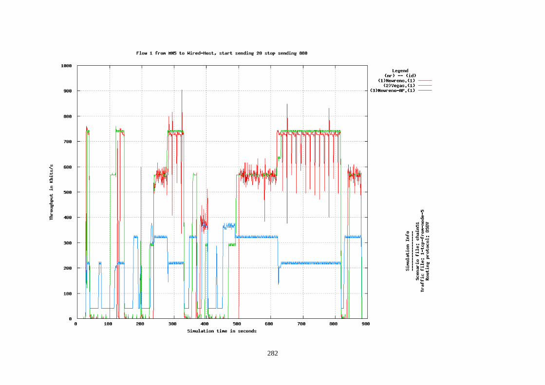
282
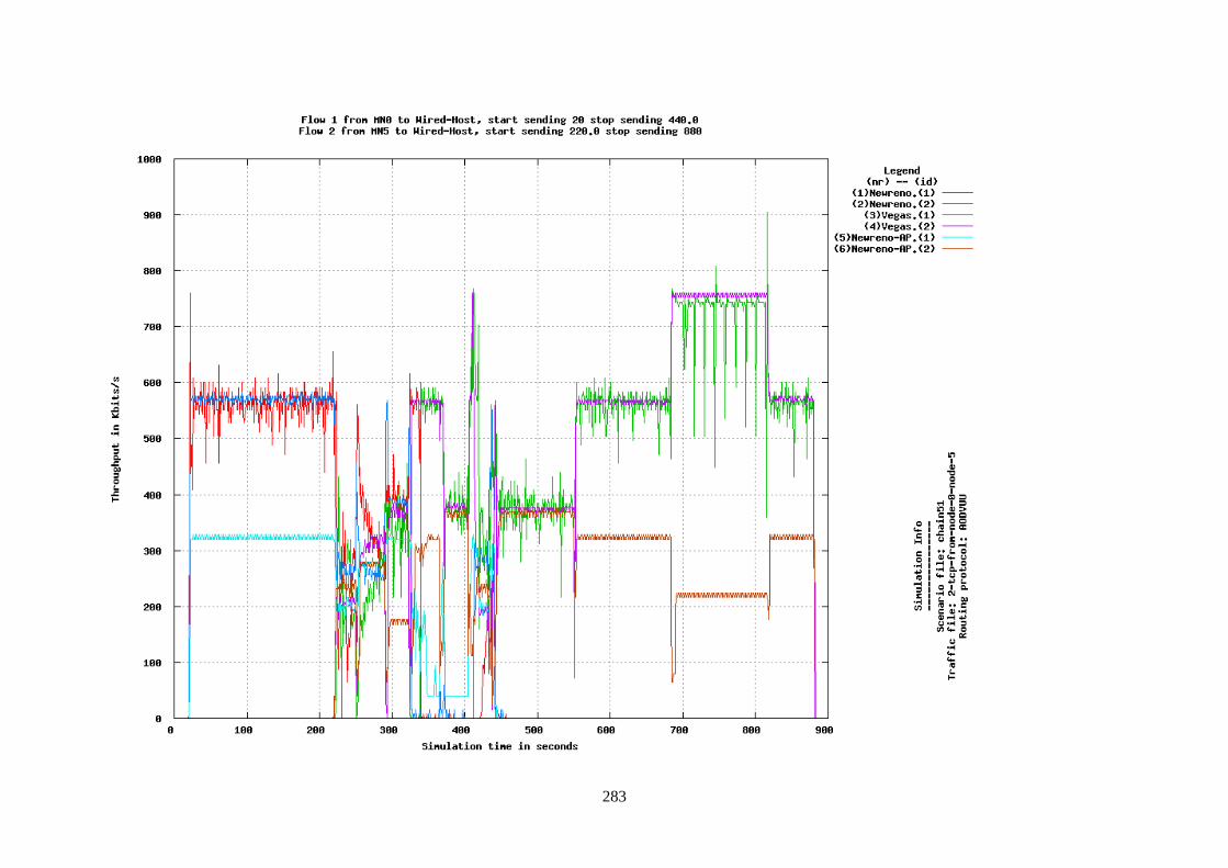
283
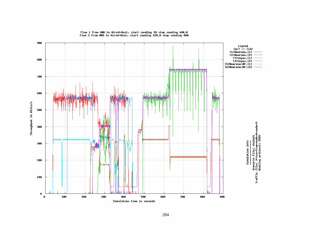
284
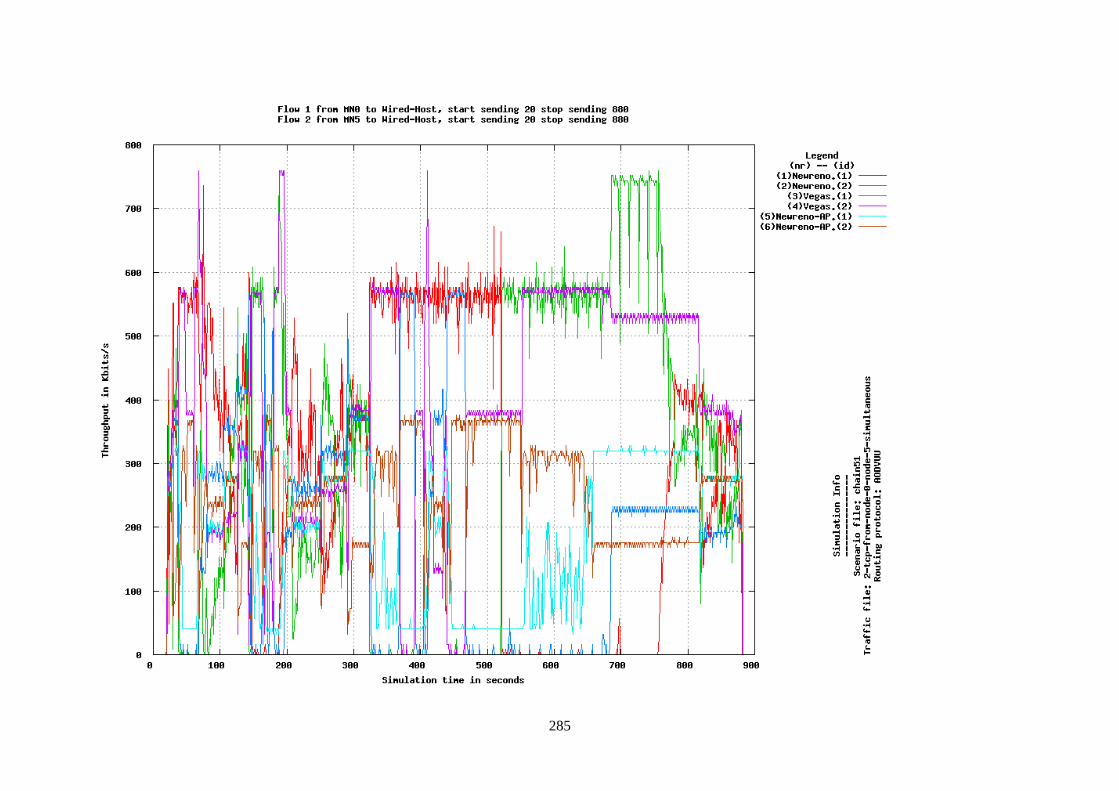
285
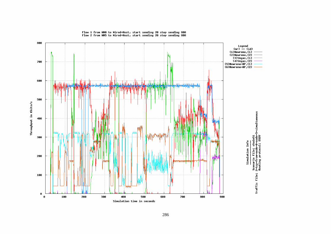
286
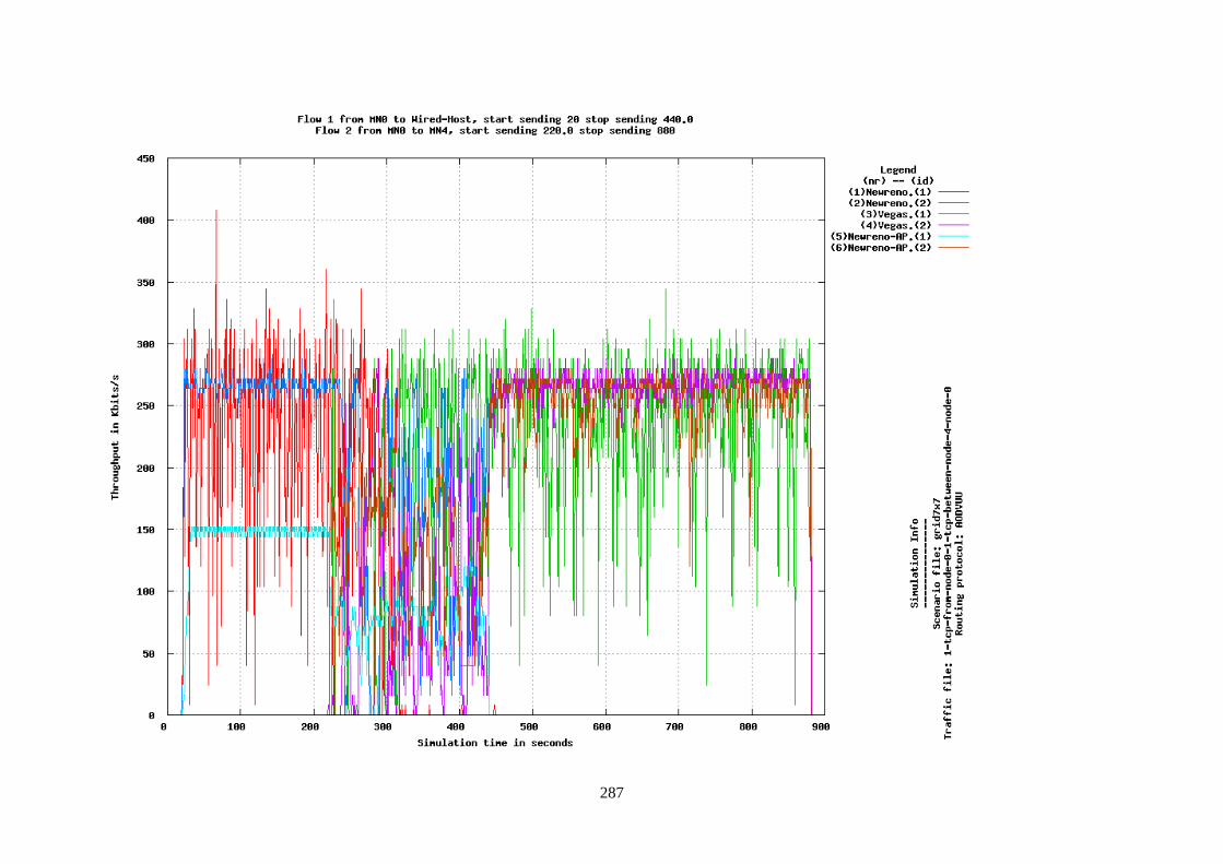
287
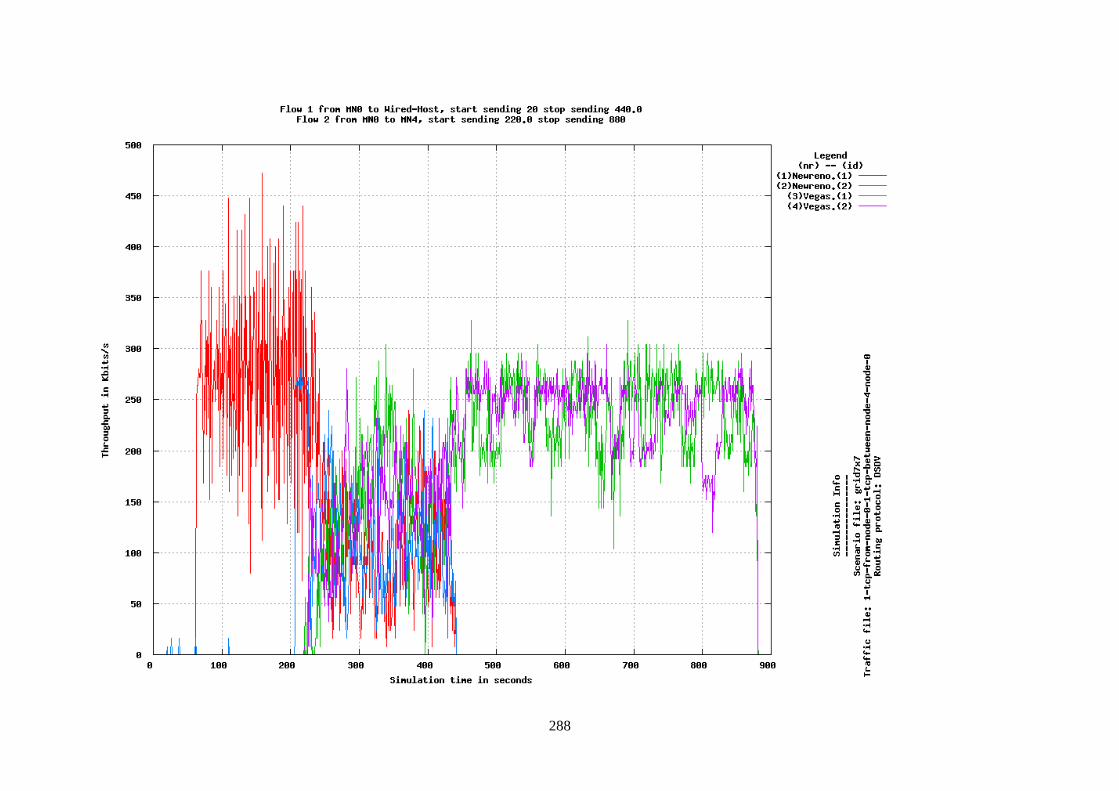
288
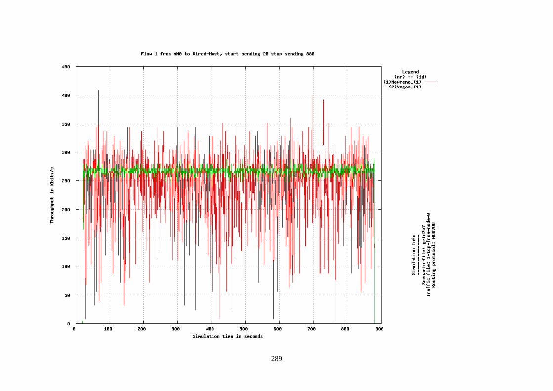
289
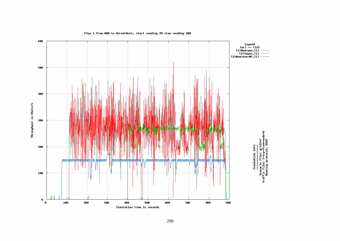
290
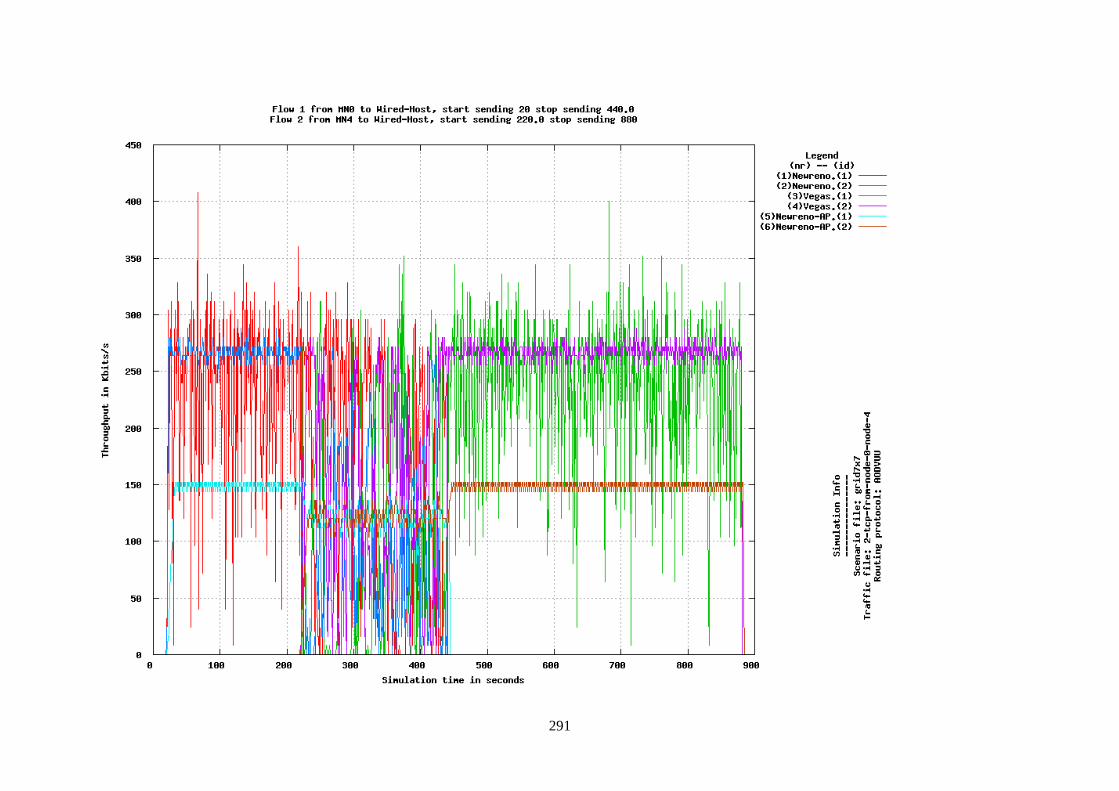
291
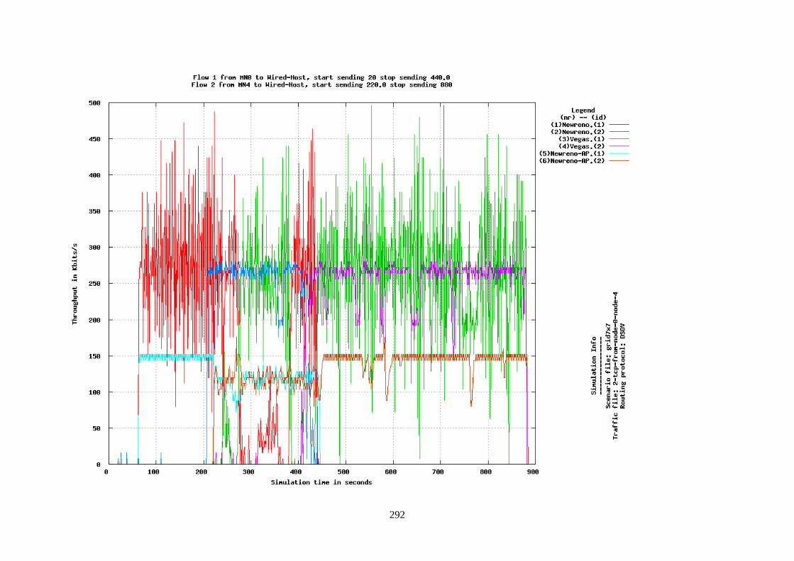
292
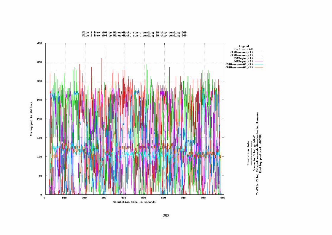
293
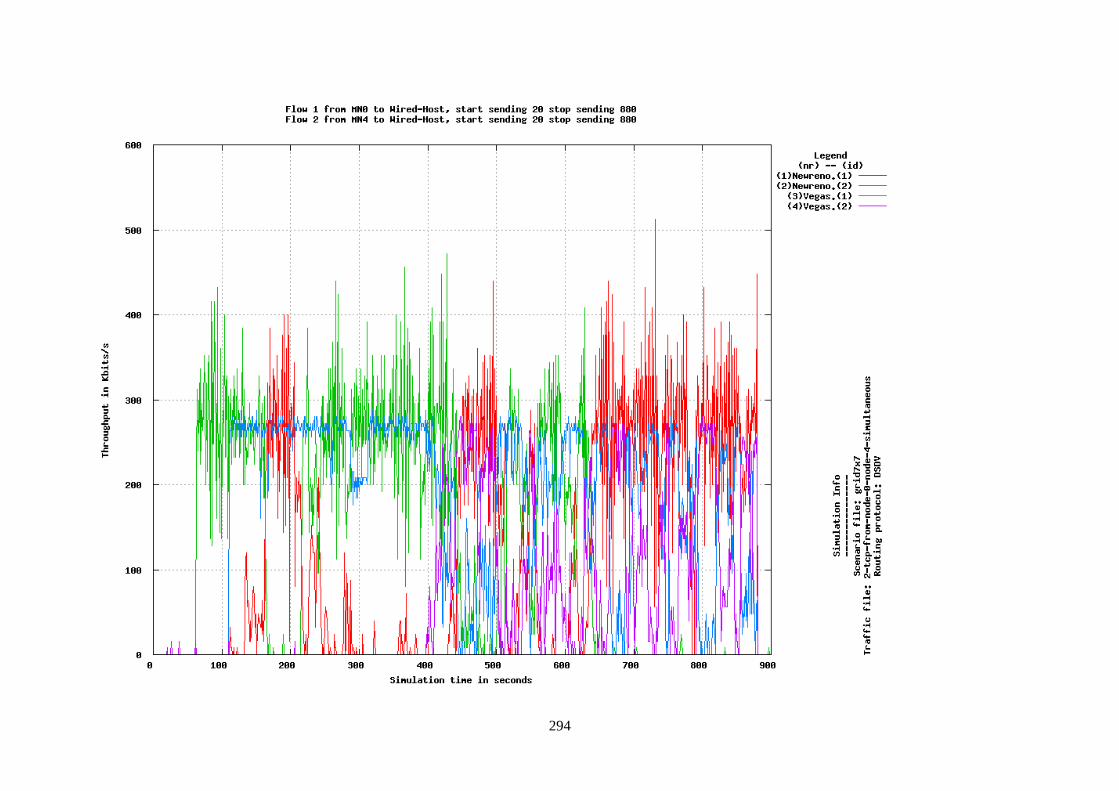
294
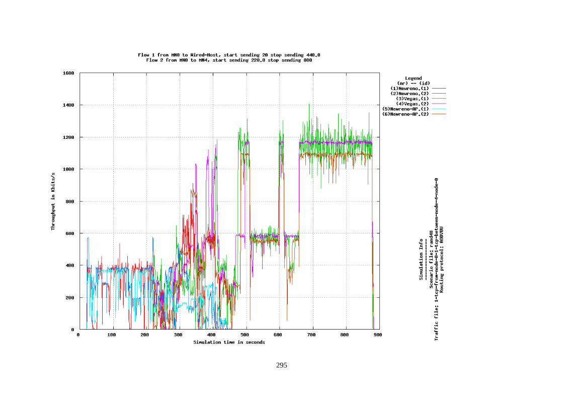
295
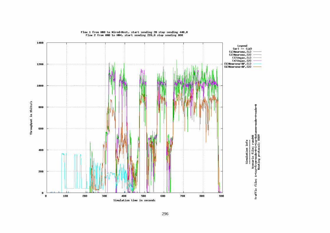
296
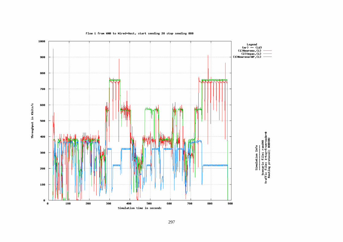
297
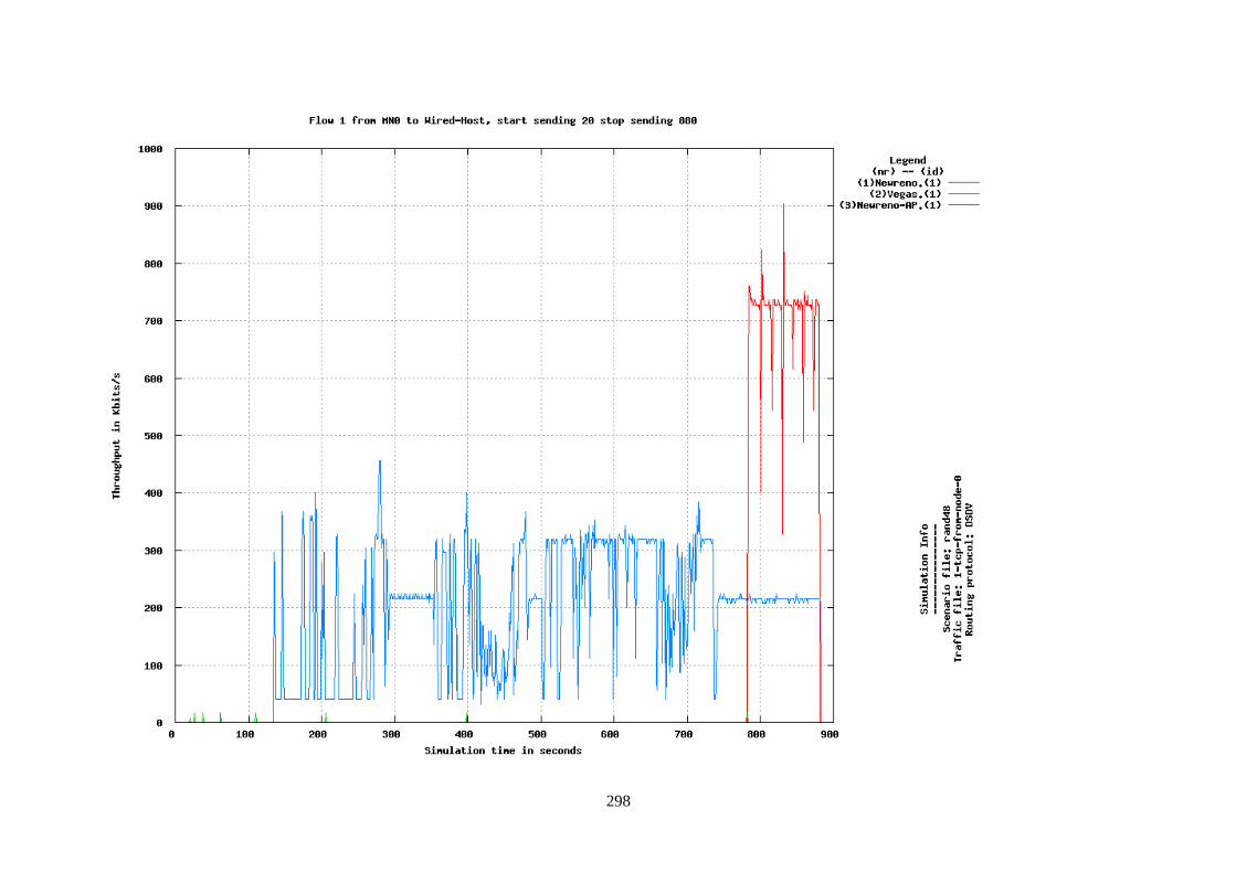
298
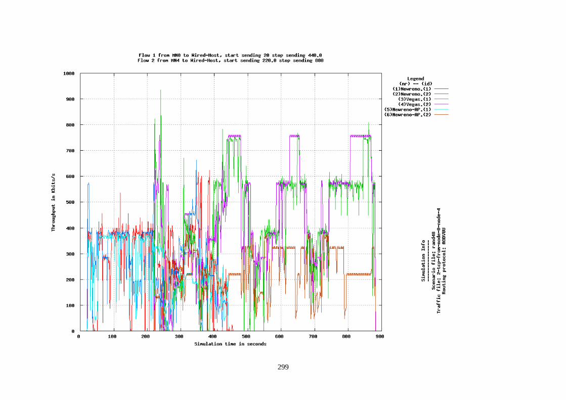
299
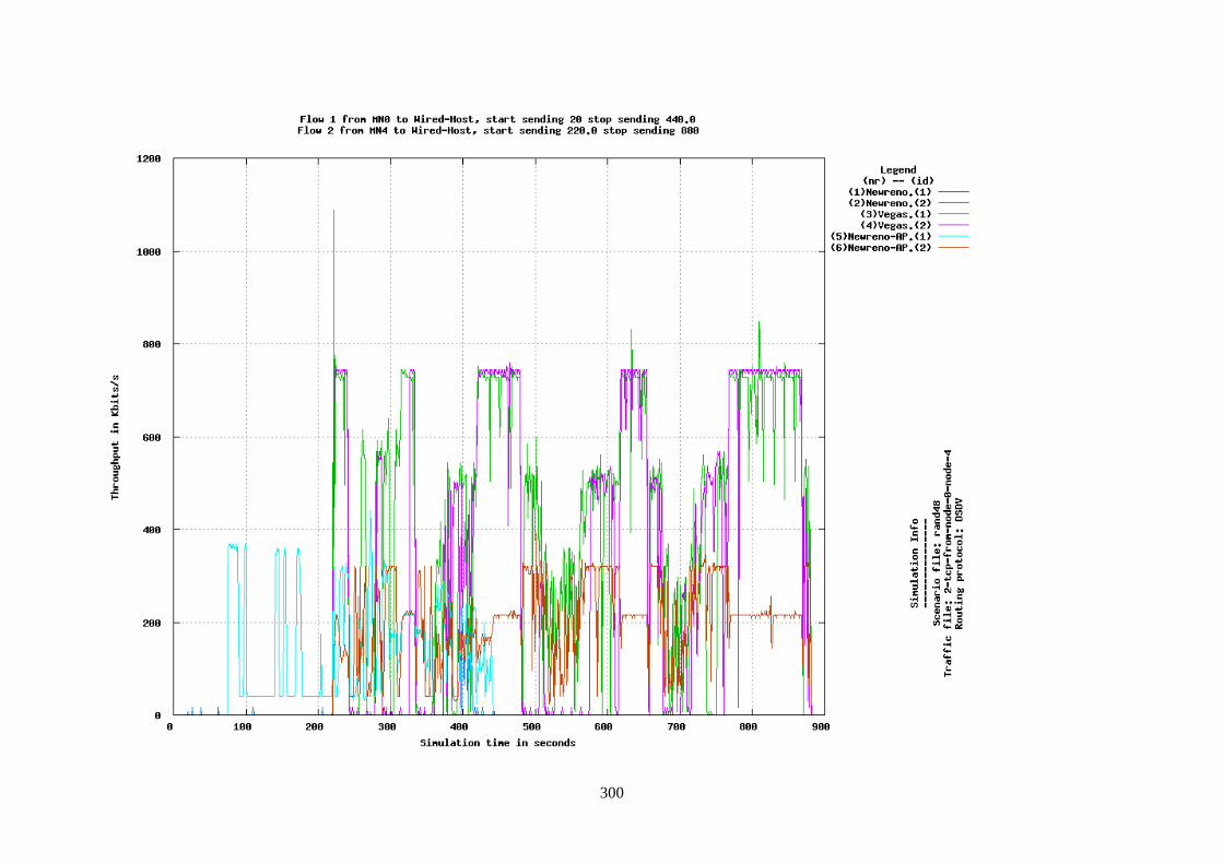
300
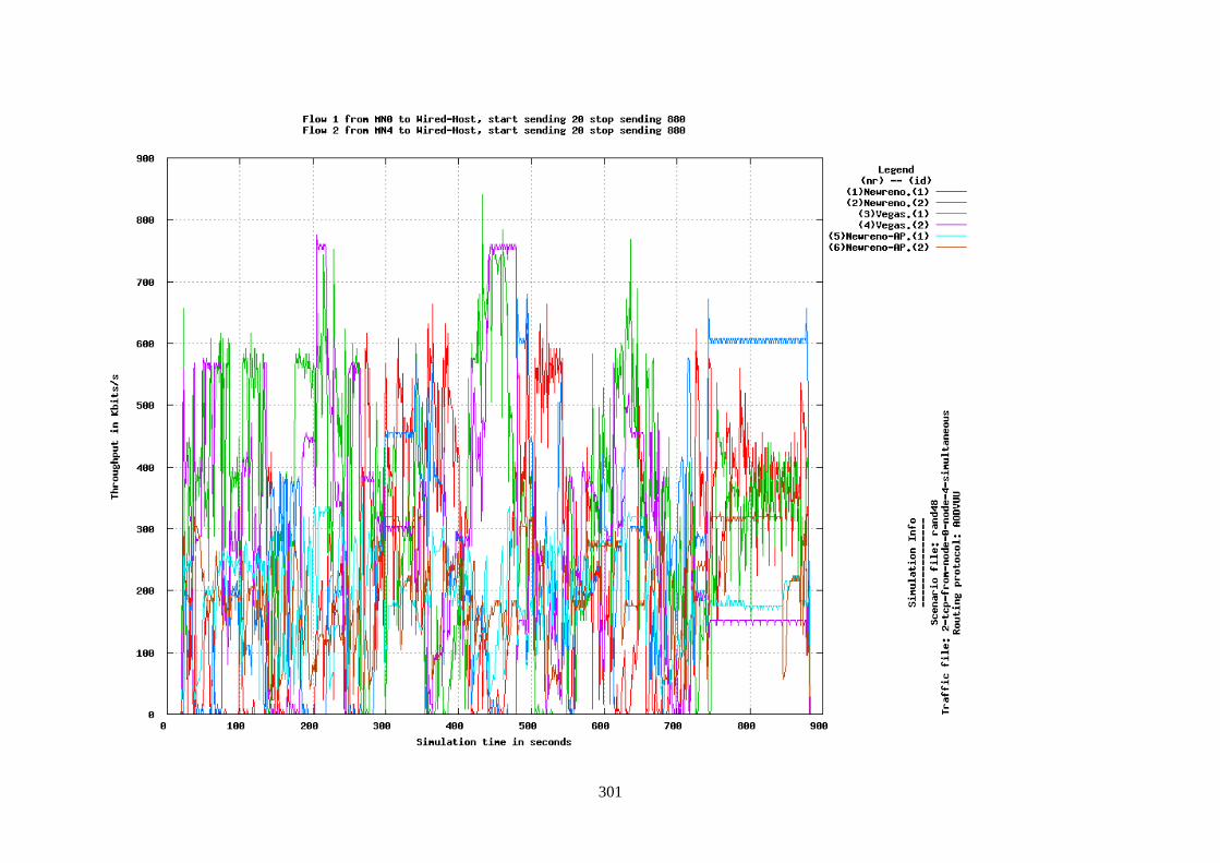
301
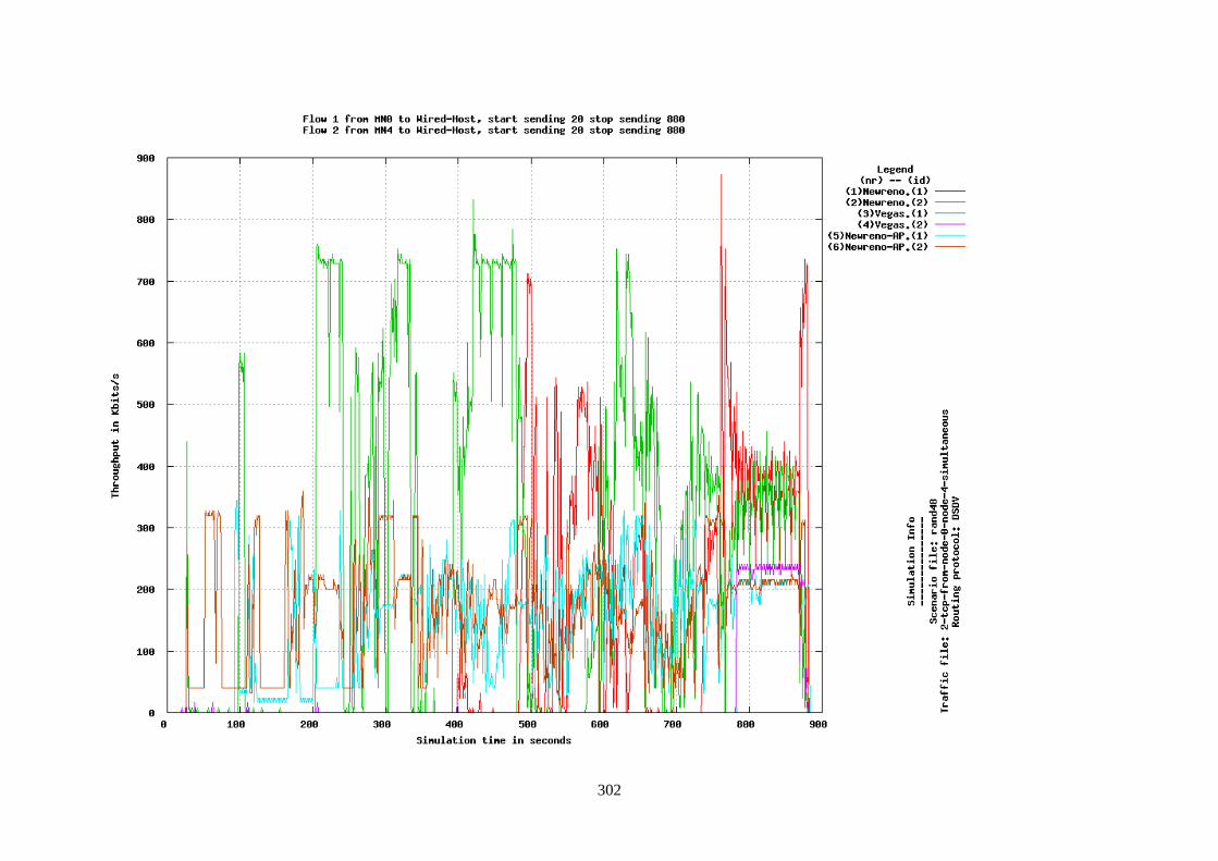
302
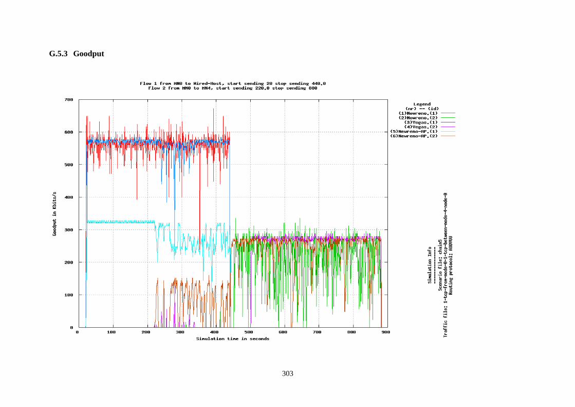
303
G.5.3 Goodput
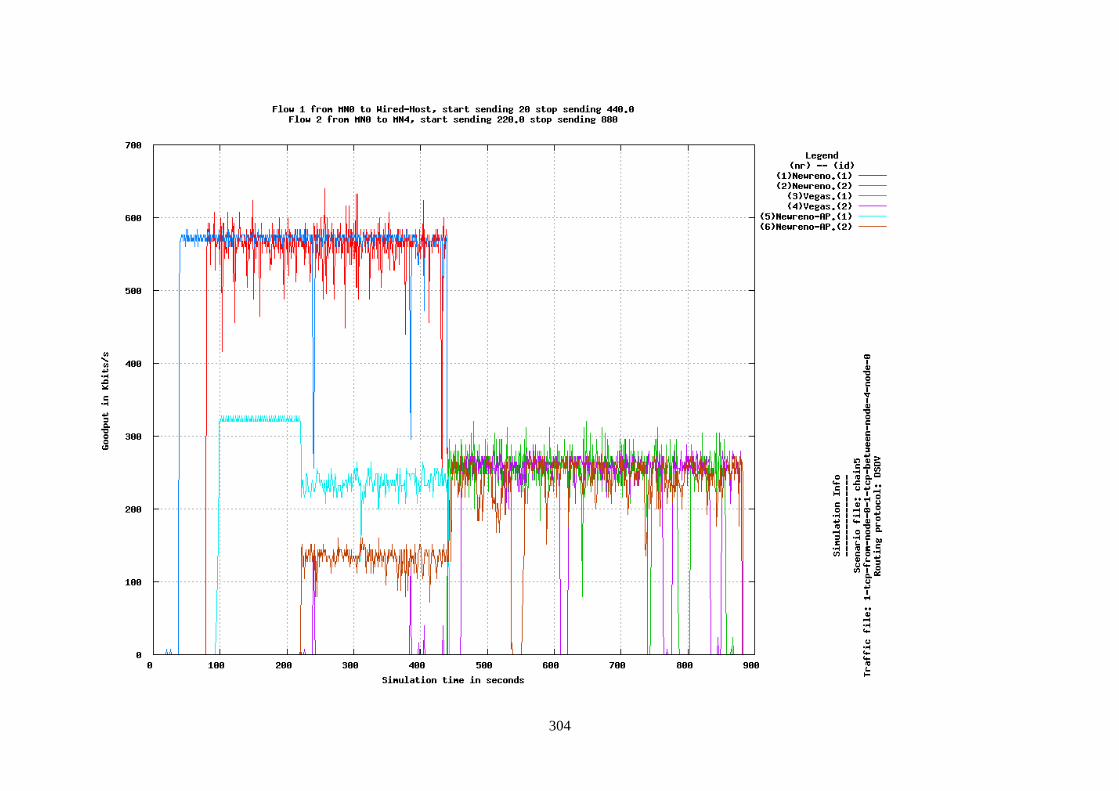
304
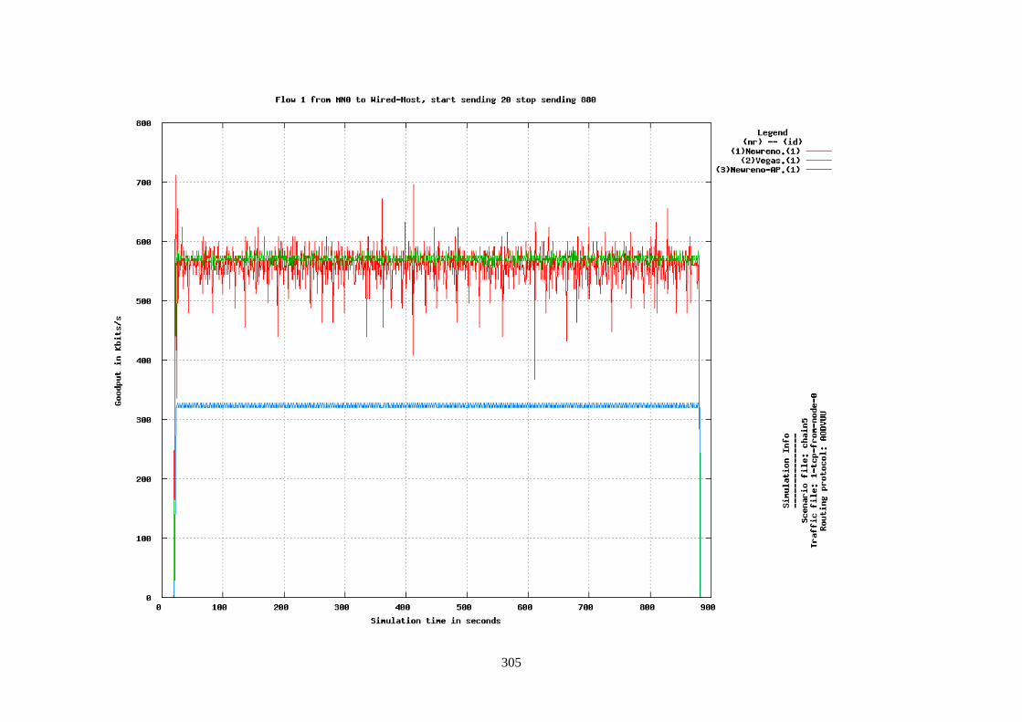
305
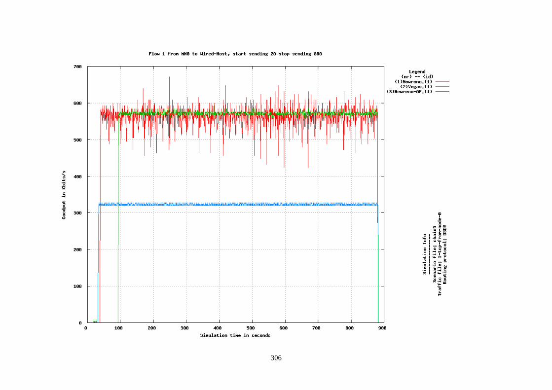
306
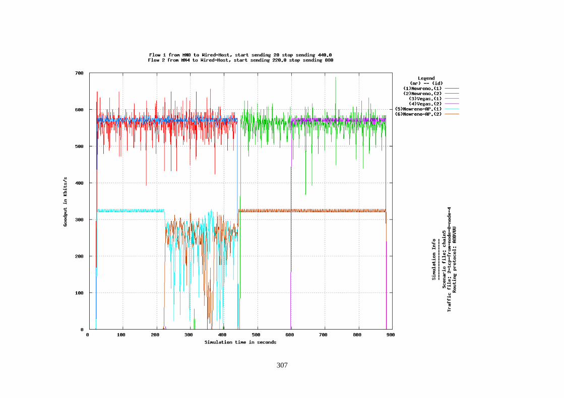
307
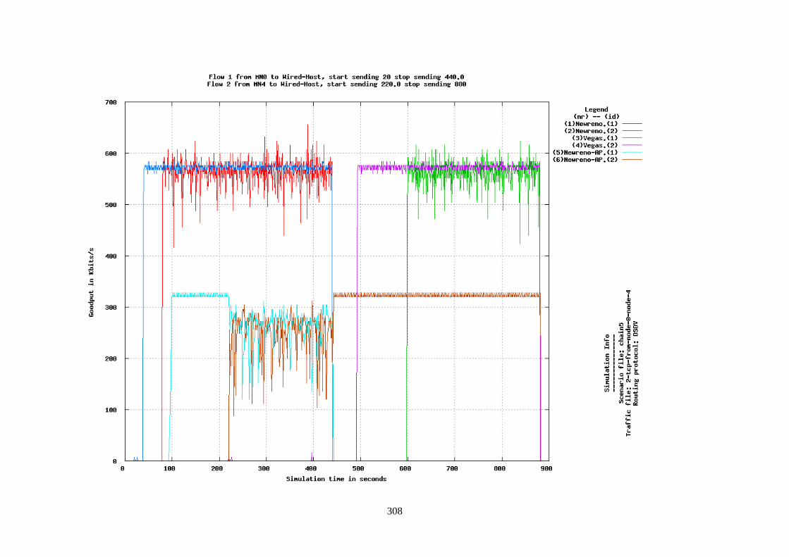
308
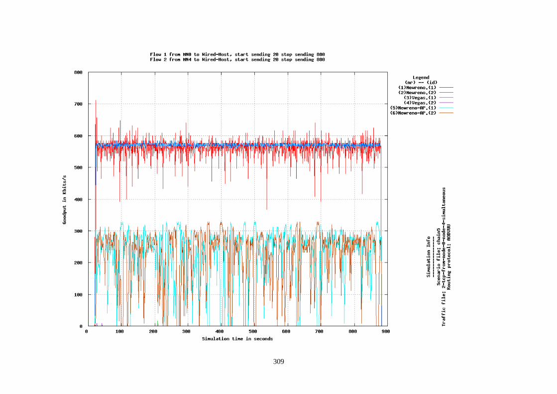
309
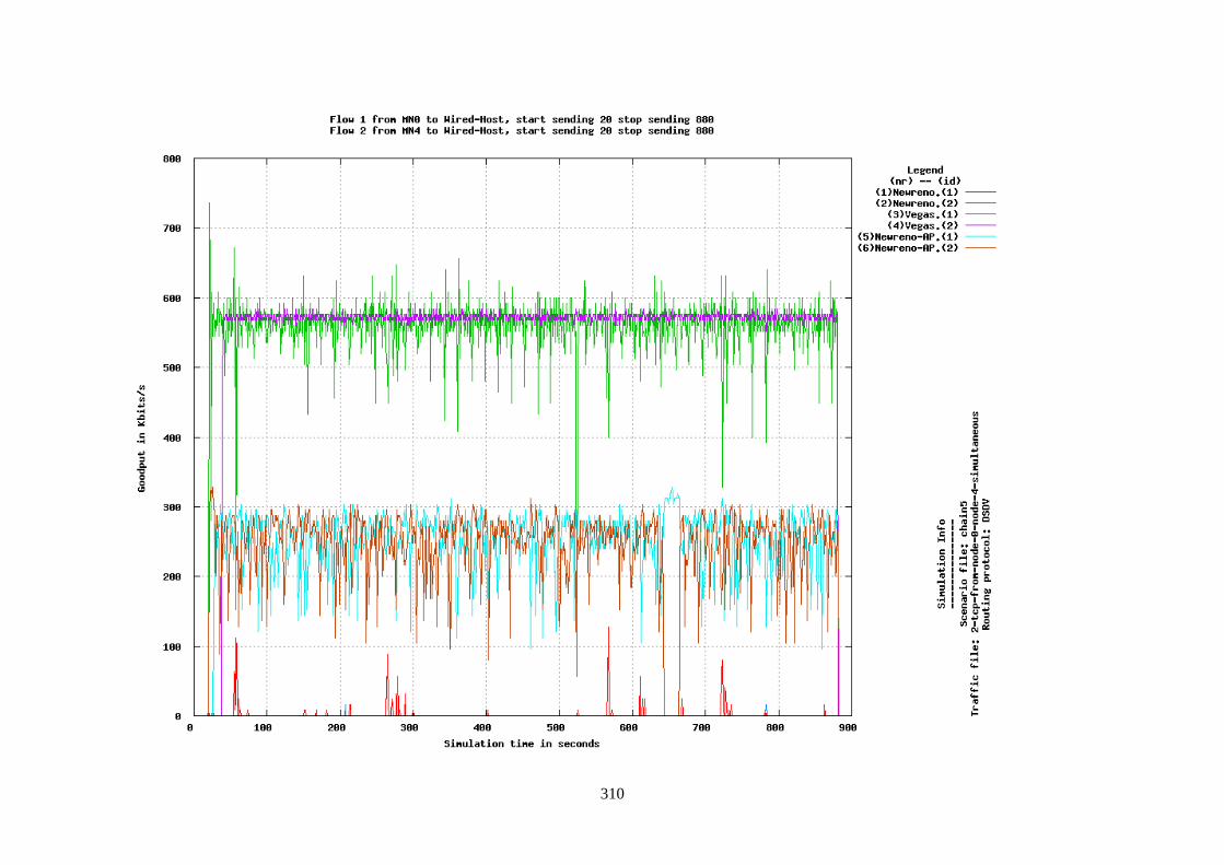
310
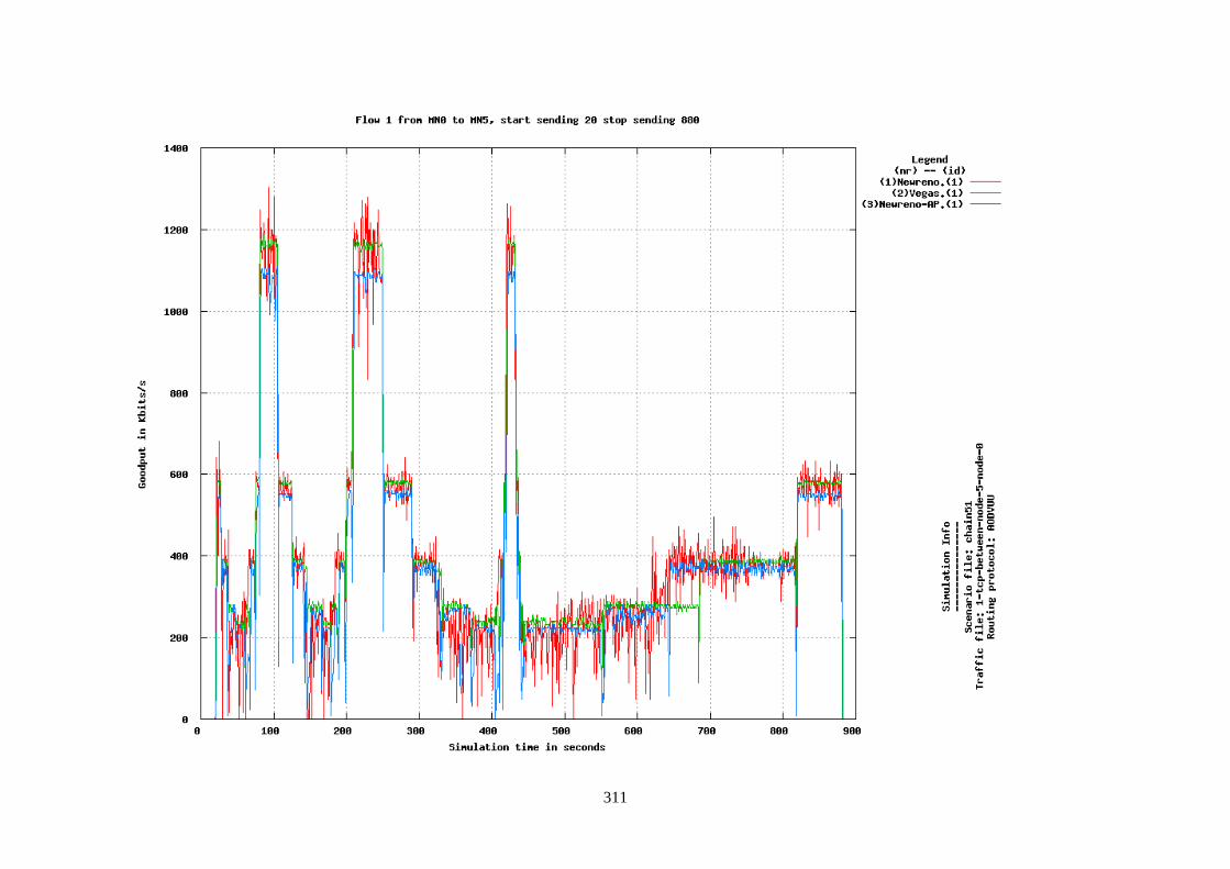
311
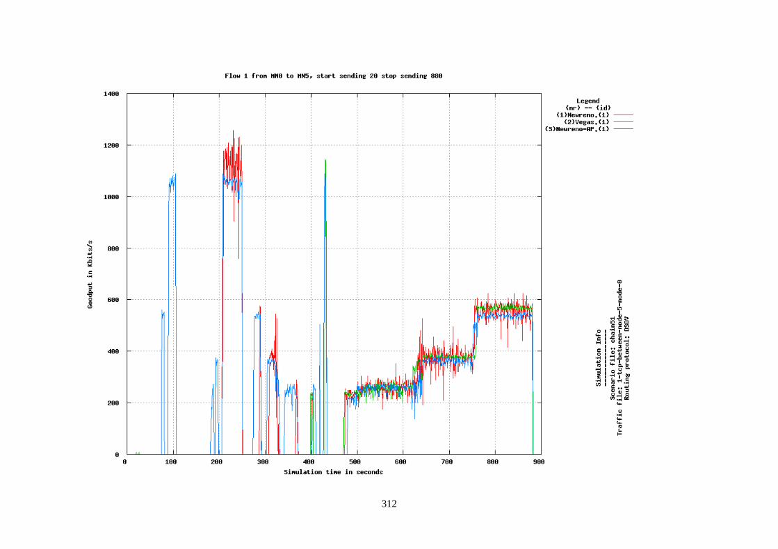
312
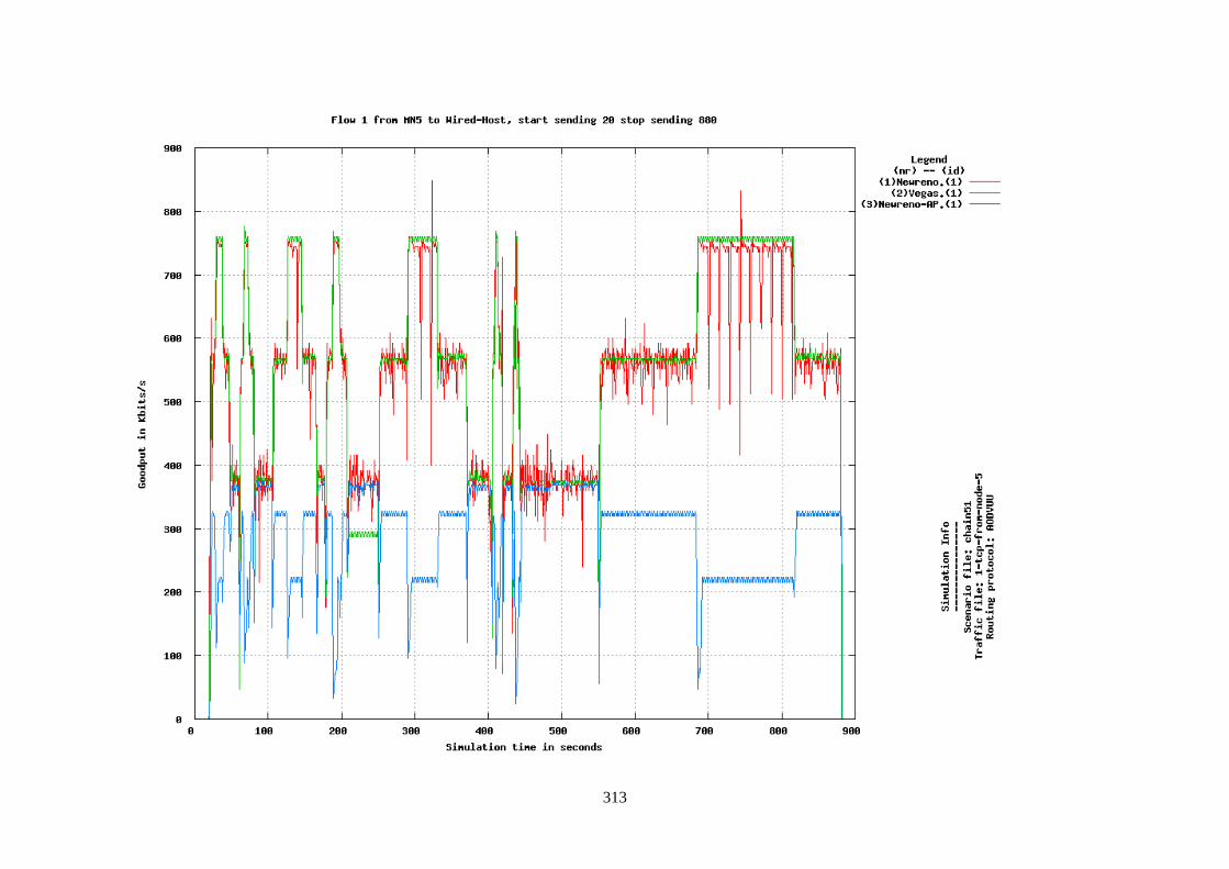
313
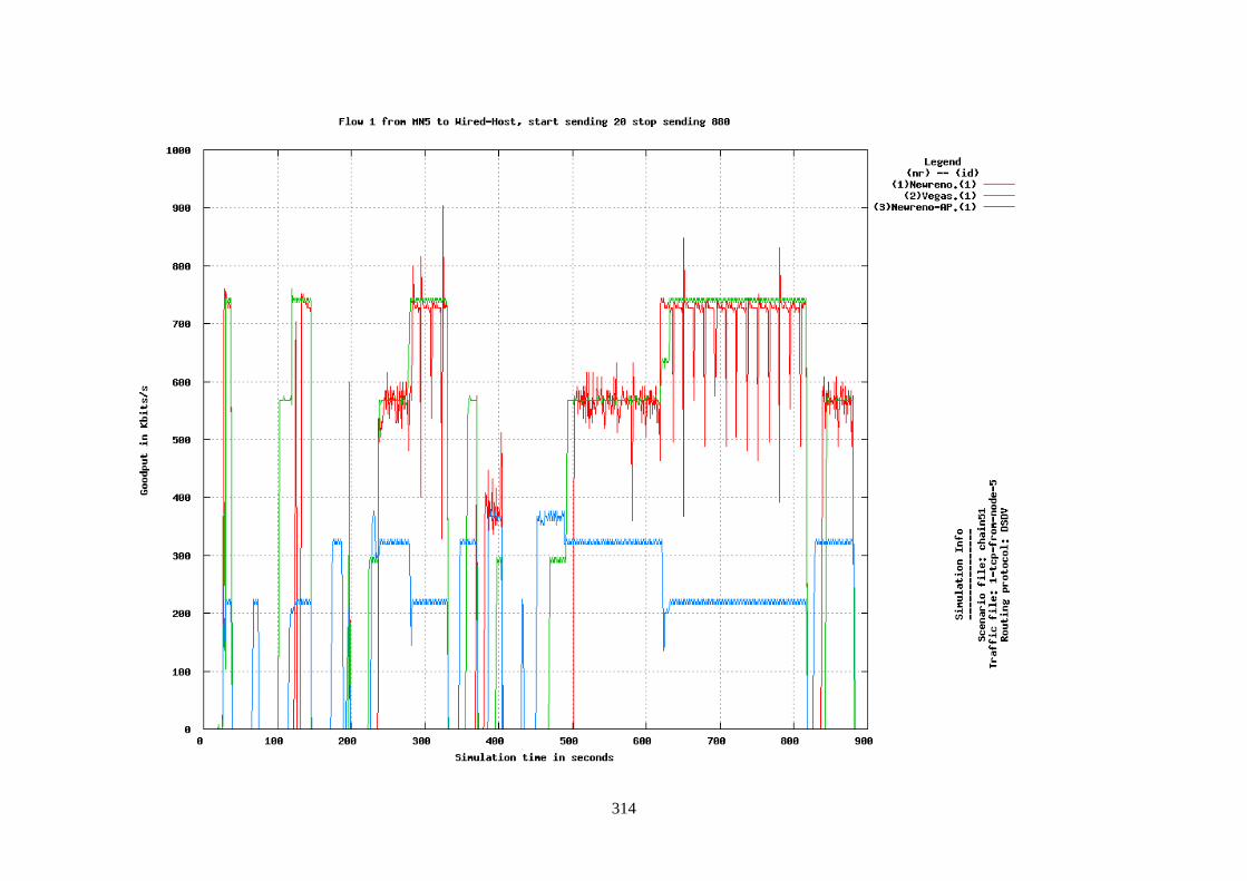
314
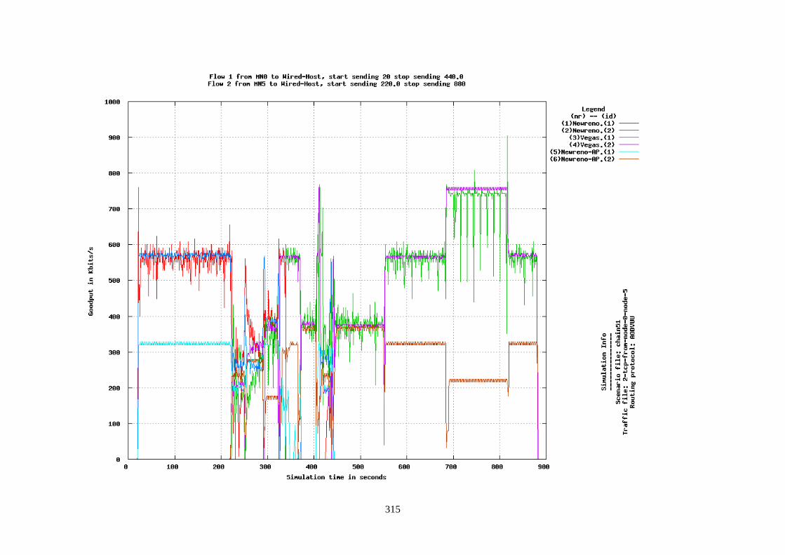
315
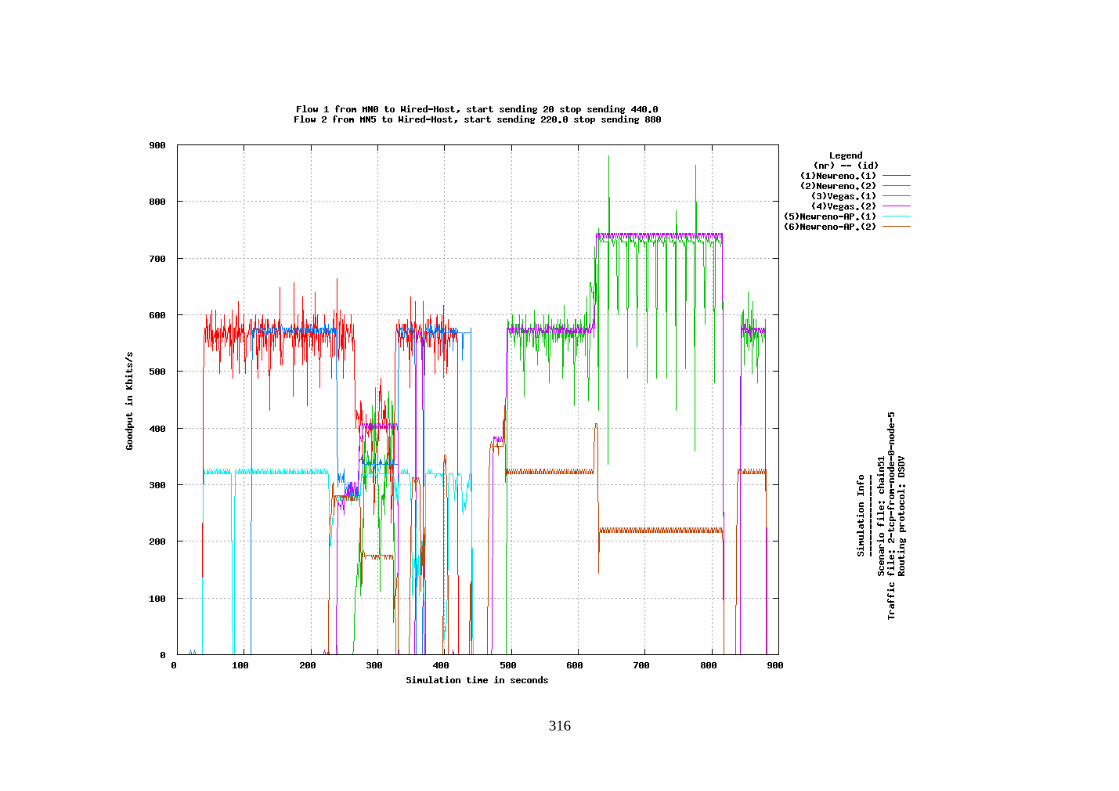
316
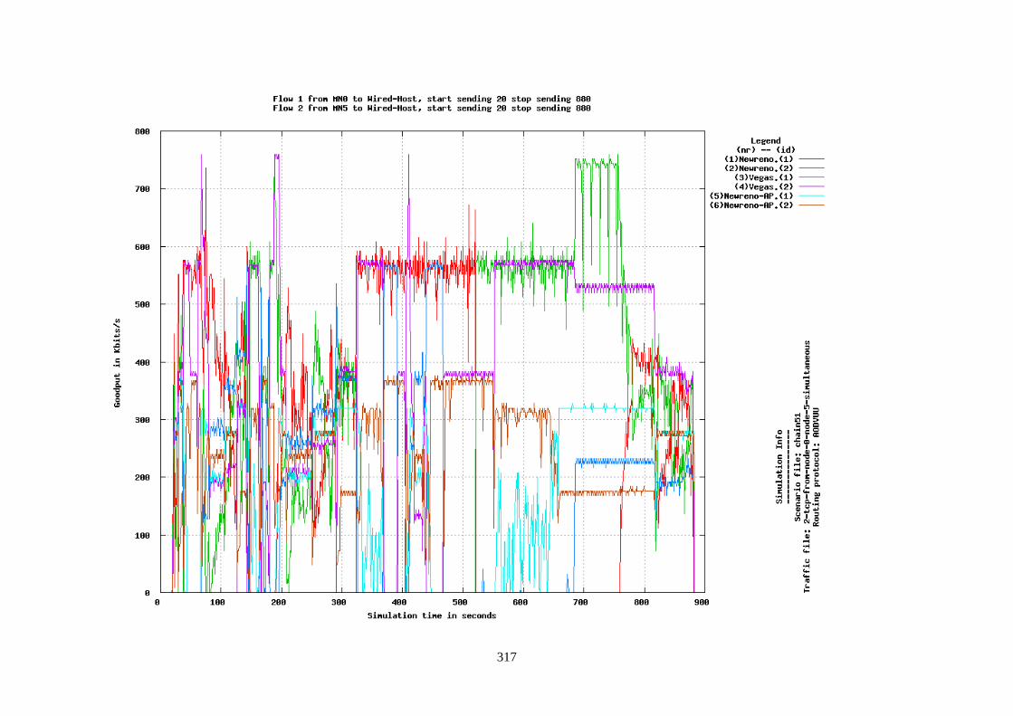
317
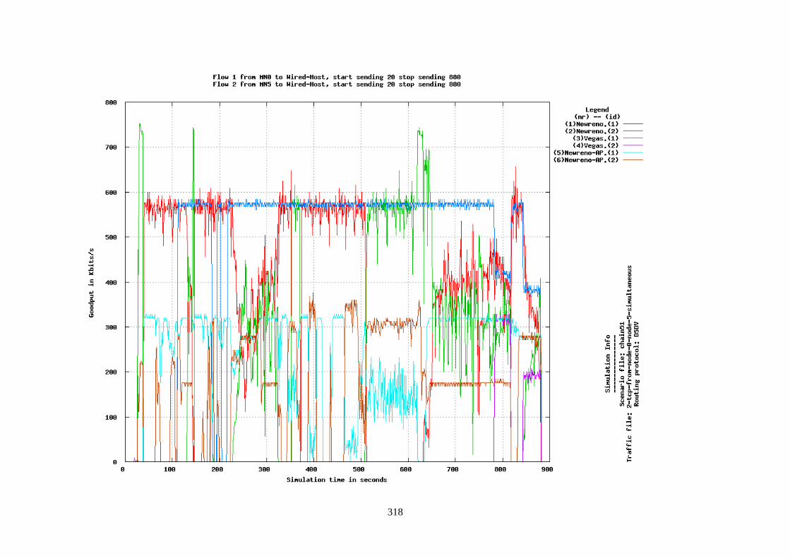
318
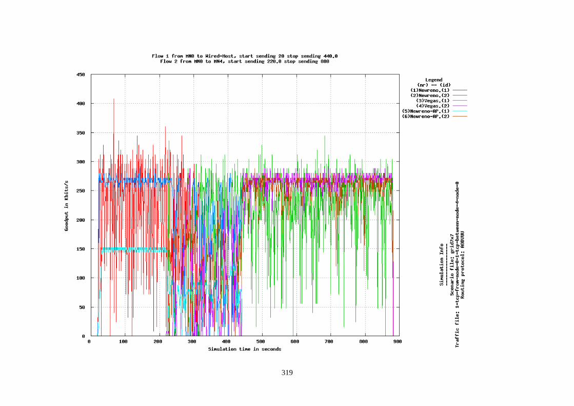
319
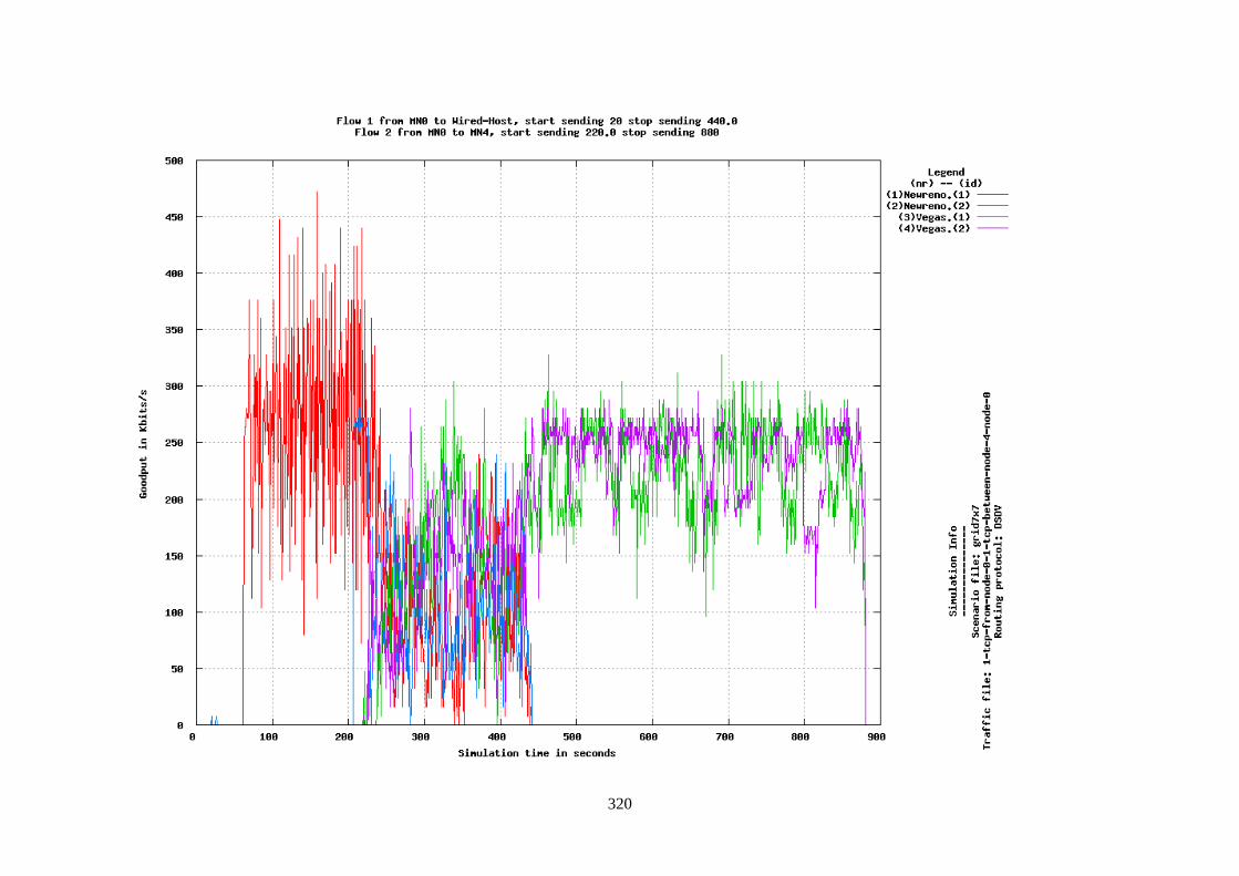
320
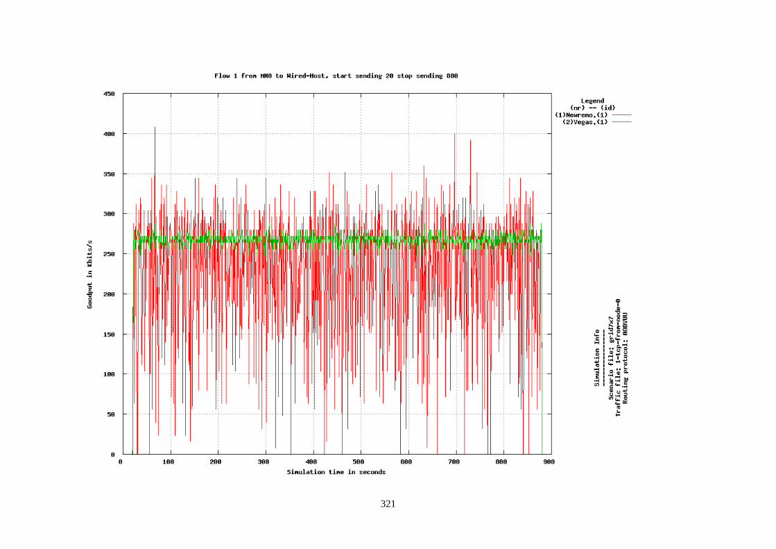
321
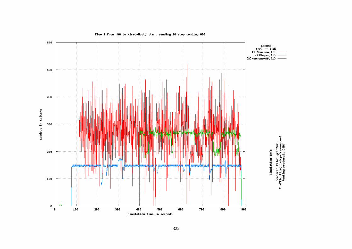
322
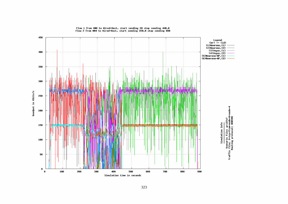
323
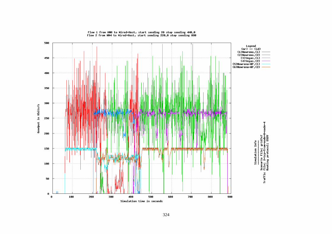
324
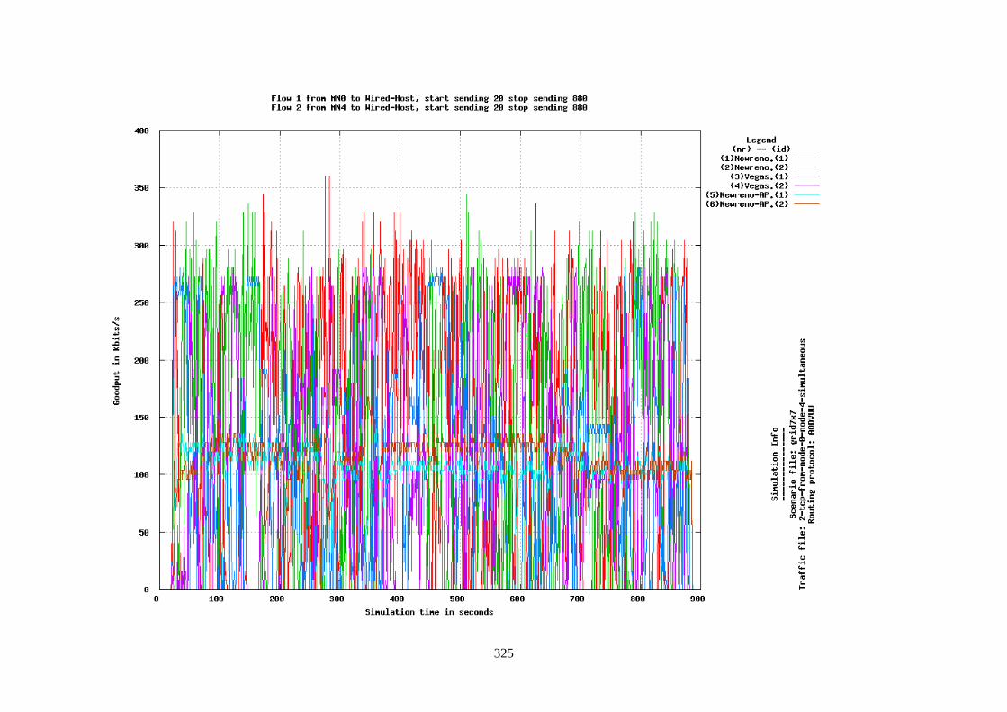
325
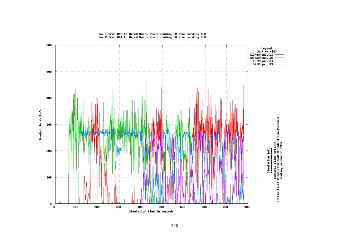
326
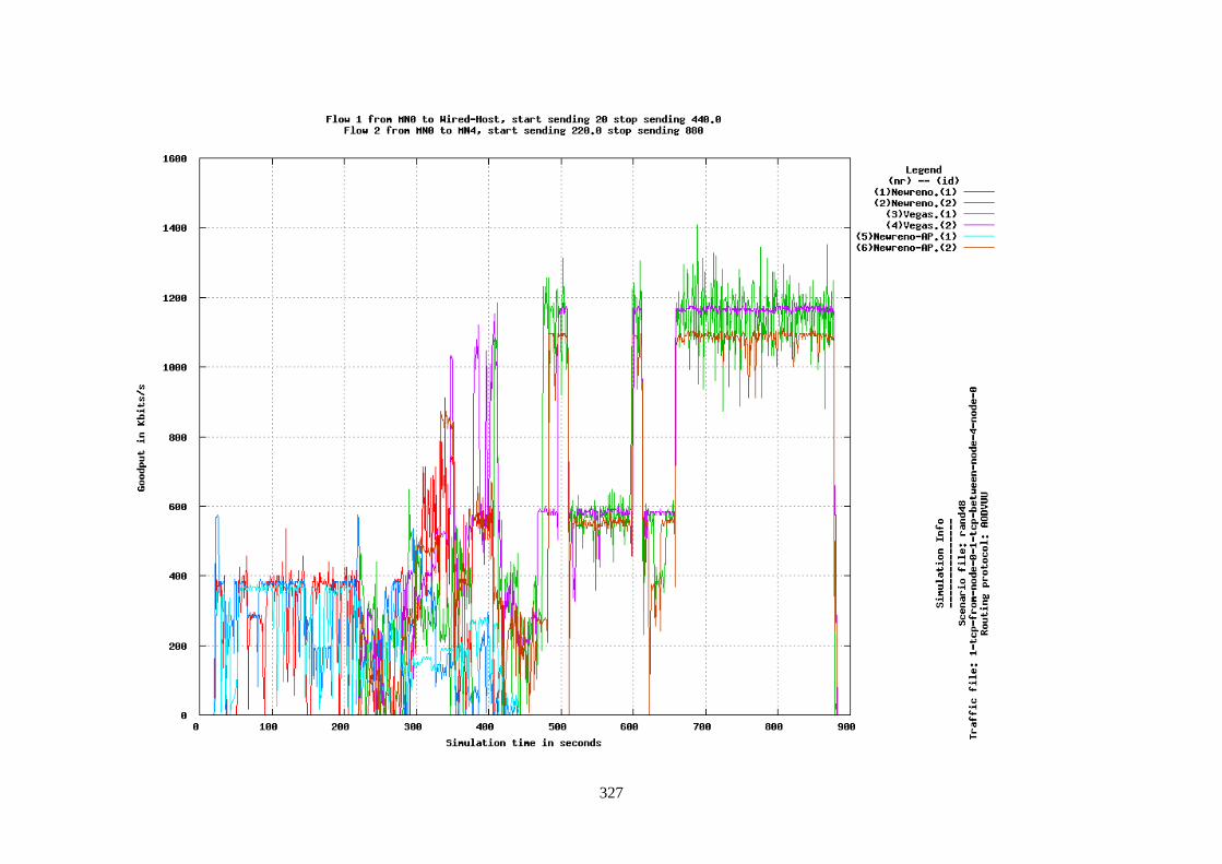
327
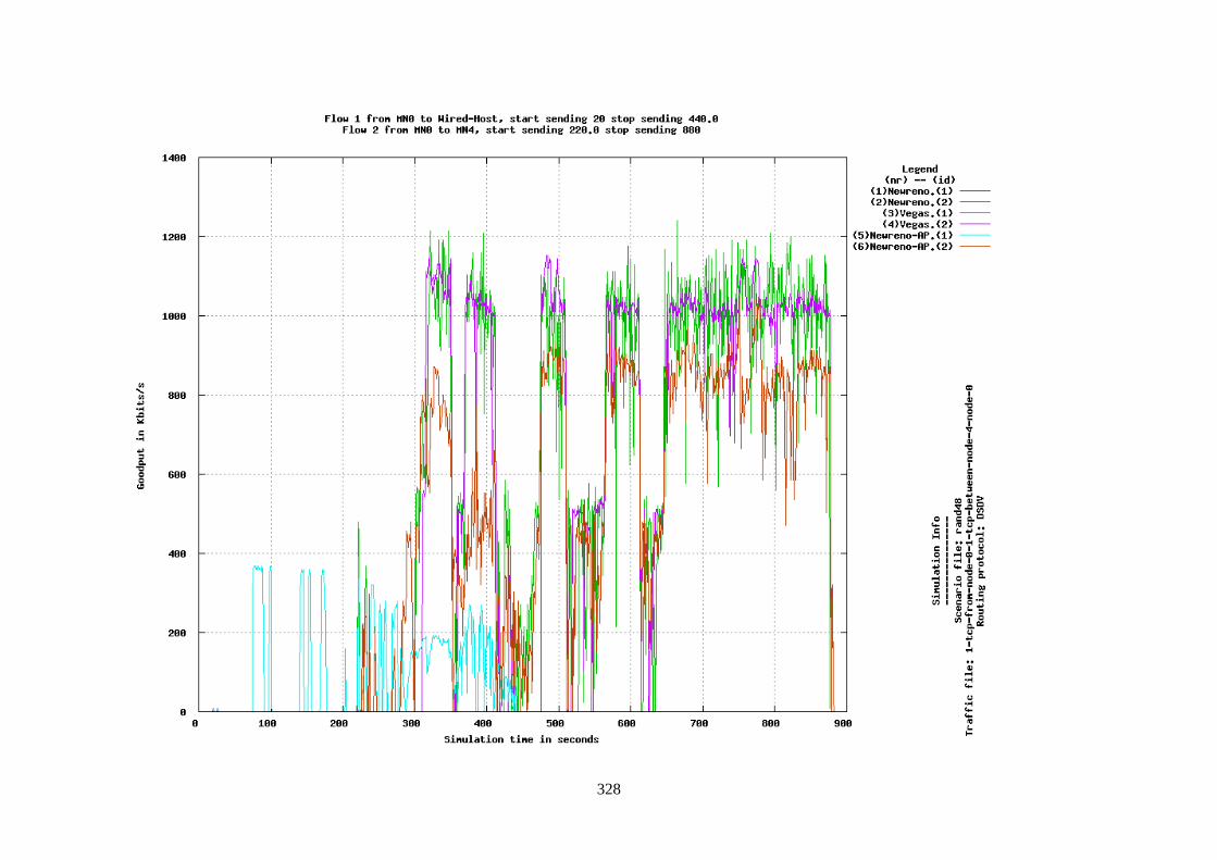
328
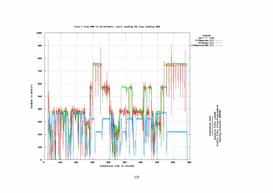
329
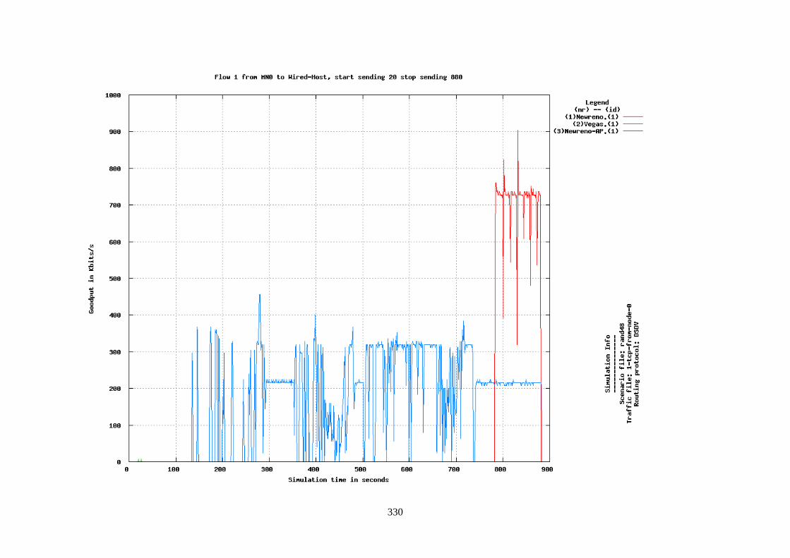
330
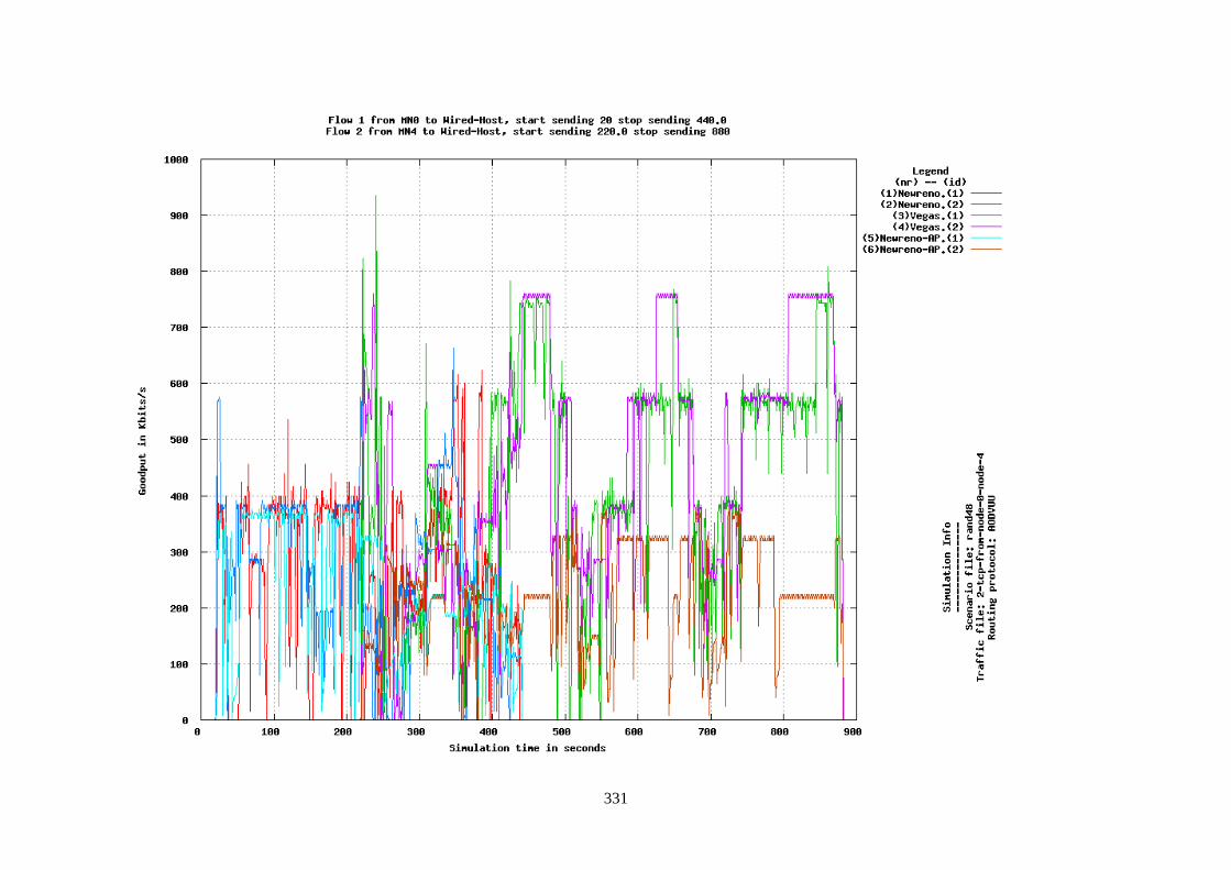
331
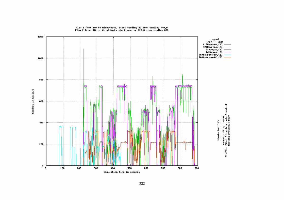
332
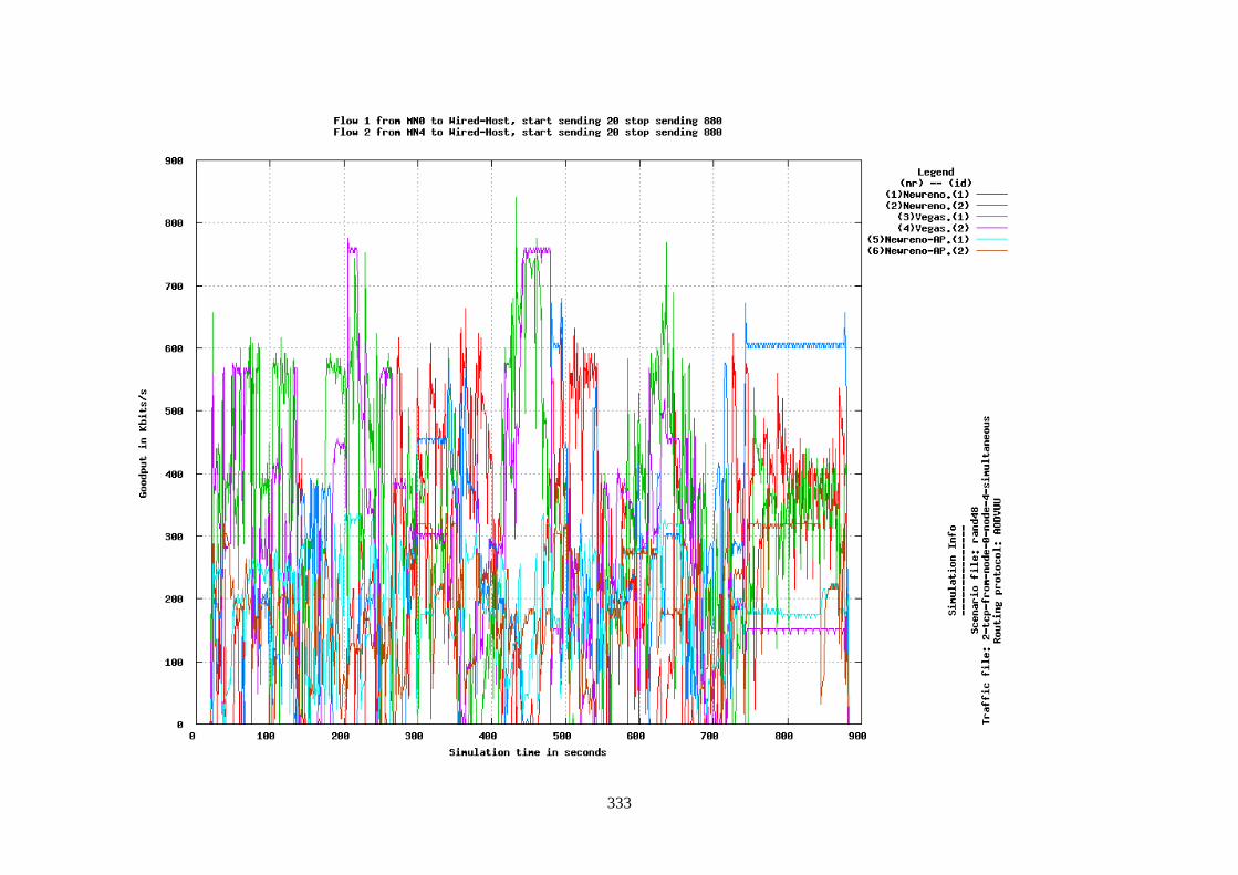
333
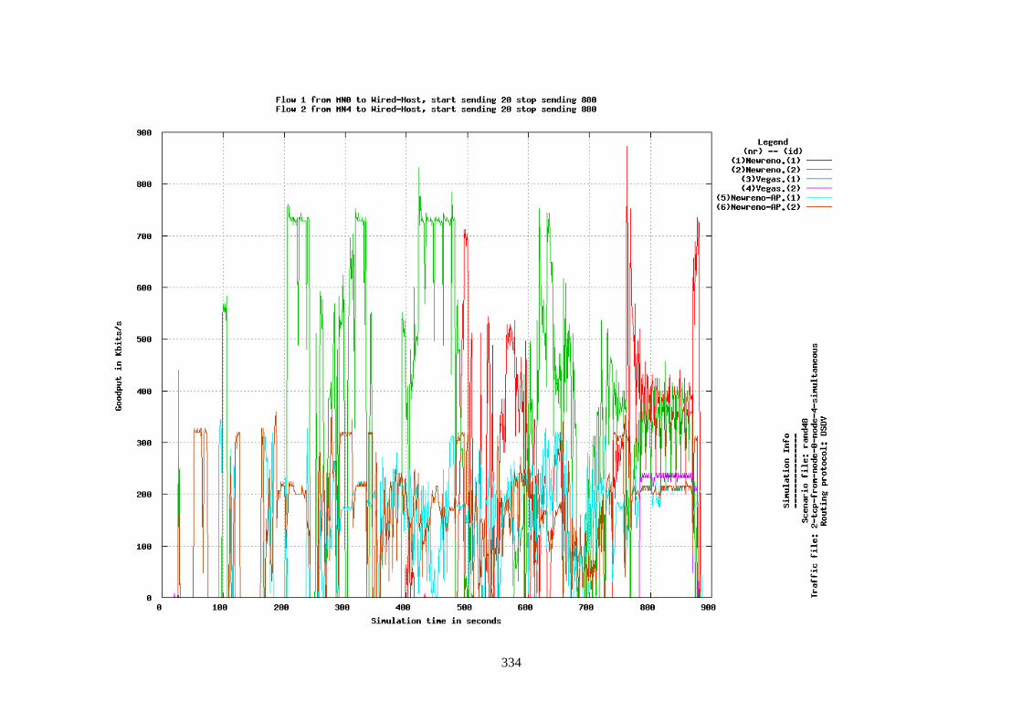
334