JOURNALOF Monetary ECONOMICS

ELSEVIER Journal of Monetary Economics 34 (1994) 47-73

Post hoc ergo propter once more An evaluation of ‘Does monetary policy matter?’ in the

spirit of James Tobin

Kevin D. Hoover*, Stephen J. Perez

Department qf’ Economics. Unicersity of Cul$omia, Davis, CA 95616-8578, USA

(Received September 1991; final version received September 1992)

Abstract

Christina and David Romer’s paper ‘Does Monetary Policy Matter?’ advocates the so-called ‘narrative’ approach to causal inference. We demonstrate that this method will not sustain causal inference. First, it is impossible to distinguish monetary shocks from oil shocks as causes of recessions. Second, a world in which the Fed only announces intentions to act cannot be distinguished from one in which it in fact acts. Third, the techniques of dynamic simulation used in the Romers’ study are inappropriate and quantitatively misleading. And, finally, their approach provides no basis for establishing causal asymmetry.

Key \+wds: Monetary policy; Economic methodology; Business fluctuations

JEL class@ficafion: B41; Cl9; E32; E52

On the fatal night of Doria’s collision with the Swedish ship Gripsholm, off Nantucket in 1956, the Irrdv retired to her cabin and.f(icked a light switch. Suddenly there was a great crash, and grinding

*Corresponding author.

We are grateful to Christina and David Romer for providing us with the data from their paper. We

appreciate the detailed comments of Thomas Mayer, James Hartley, Kevin Salyer, and the partici- pants in the U.C. Davis Macroeconomics Brownbag Workshop. We are also grateful to Milton Friedman, James Hamilton, Neil Ericsson, an anonymous referee, and to the participants in

seminars at the Federal Reserve Bank of St. Louis, the Board of Governors of the Federal Reserve

System, Old Dominion University, and the University of North Carolina, Chapel Hill, for many

helpful comments.

0304-3932/94/$07.00 0 1994 Elsevier Science B.V. All rights reserved SSDI 030439329401 149 2

48 K.D. Hoover, S.J. Perez 1 Journal of Monetary Economics 34 (1994) 47- 73

metal, and passengers and crew’ ran screaming through the passageways. The lady burst,from her cabin and explained to the first person in sight that she must have set the ship’s emergency brake! David Hackett Fischer. Historians Fallacies’

1. Introduction

The causal direction between money and income has been debated since modern economics began in the last quarter of the 18th century. Professional allegiances have waxed and waned, demonstrating that there are cycles of economic thought as well as of trade. When Friedman and Schwartz first made their case in favor of the priority of money, it was ‘Keynesians’ who argued that money did not matter. Among classically minded macroeconomists, the new classical school has over time captured centerstage, pushing monetarism into the wings.’ As the focus of the new classical macroeconomics has shifted towards equilibrium real-business-cycle models, some new classicals argue that money is merely an epiphenomenon, and it is the new Keynesians who now argue strenuously that money matter.3

This shift of opinion has engendered a new respect for the work of Friedman and Schwartz among new Keynesians. Christina and David Romer’s ‘Does Monetary Policy Matter? A New Test in the Spirit of Friedman and Schwartz’ (1989) is symptomatic of the latest cycle in professional opinion. In their paper, the Romers critically reevaluate Friedman and Schwart’z interpretation of interwar U.S. economic history, and they attempt to use modern statistical methods (leavened with old-fashioned narrative) to extend Friedman and Schwartz’s work to the interpretation of post-World War II economic history. In this essay, we focus on the methodology applied by the Romers to the postwar period: the claim that combining narrative information with modern statistics ‘. . . can solve the problem of identifying the direction of causation between monetary factors and real economic developments’ (p. 167).4

If the Romers’ claim is correct, it is an important advance in economic methodology. We do not ourselves wish to make any substantive claim about causal direction. Rather, as Tobin (1970) did for Friedman and Schwartz (1963a,b), we want to inject a cautionary note about empirical methodology: the

r We thank Gilbert Yochum for drawing this passage to our attention.

*Many see the new classical macroeconomics as the natural successor to monetarism. The dimensions in which that is true make it an interesting thesis. Still, the differences between

monetarists and new classicals are more profound than their similarities. See Hoover (1984) or

Hoover (1988, Ch. 9).

%ee Blanchard (1990) for a survey of reasons why money might affect output

4All citations to Romer and Romer (1989) are by page number only.

K.D. Hoooer. S.J. Perez 1 Journal qf Monetary Economics 34 (1994) 47- 73 49

methods that the Romers advocate can tell us nothing about causal direction; they are rather just another version of the fallacy post hoc ergo propter

hoc.’ We offer three arguments against the Romers’ method. Although the argu-

ments are sufficiently independent that acceptance of any one of them is enough to undermine the Romers’ claim to have solved the problem of causal inference, they are nonetheless mutually supporting.

First, we show that their narrative/statistical approach cannot discriminate between monetary and nonmonetary shocks as a source of recessions by showing that oil shocks produce statistical results of precisely the same charac- ter as the monetary shocks the Romers have identified. The point is not that we believe that oil shocks really are the cause of all recessions; rather it is that, conditional on the validity of the Romers’ approach, an investigator who focussed on oil shocks would find the same support for them as the Romers find from monetary shocks. Furthermore, once oil shocks are seen as a primafacie

alternative to monetary shocks, then it is easy to see that there is no convincing evidence in the Romers’ account that monetary shocks are the cause or even a joint cause of real fluctuations, and nothing to rule out that money is merely a passive responder to other shocks that really cause real fluctuations.

Second, to follow up the argument that monetary shocks may be passive responses, we use a simulation study to show that the Romers’ technique cannot discriminate between a world in which the Federal Reserve can actually induce recessions and one in which it merely declares an intention to induce a recession without taking any effective action to realize that intention.

Third, we demonstrate in theory and practice that dynamic simulation methods are inappropriate for causal inference and quite misleading as guides to the quantitative effects of any policy action.

Any one of the three arguments we offer undermines the Romers’ method. But our aim is not wholly negative. We provide a sketch of an alternative method for causal inference. This gives further insights into why the Romers’ method cannot be successful. It is important to recall that we take no substantive position on whether money matters. Our aim is methodological: even if money does matter, the fact that it matters cannot be established using methods similar to those advocated by the Romers.

‘Some cautionary historical notes: Friedman (1970) argues that, contrary to Tobin, he and Schwartz find timing relations of interest only after the direction of influence is established on

other grounds. Friedman (1970, p. 319) goes out of his way not to use the words ‘cause’ and ‘causal’ when speaking of the influence of money on income; see also Hammond’s (1992) interview of

Friedman.

50 K.D. Hoover, S.J. Perez / Journal cf Monetary Economics 34 (1994) 47- 73

2. The combined narrative/statistical approach

The Romers advocate what they call the ‘narrative approach’ to evaluating the causal efficacy of money over output. 6 With respect to their evaluation of Friedman and Schwartz’s interpretation of the interwar period, their approach is principally narrative. With respect to the postwar period, it combines narra- tive with time-series econometrics.’ We have no quarrel with the narrative approach per se (see Section 6 below). The problem is the way in which it is combined with econometric evidence. Our analysis is therefore restricted to the Romers’ evaluation of the postwar period.

The Romers read the Records of Policy Actions of the Federal Open Market Committee (FOMC) as well as the minutes of the FOMC, when these were available, to discover those times when the FOMC consciously decided to induce recessions in order to reduce inflation. They identify six dates which they refer to as ‘monetary shocks’: October 1947, September 1955, December 1968, April 1974, August 1978, and October 1979. The Romers excluded instances in which the FOMC wished to promote expansions because such instances are, in their view, more likely to be endogenous (pp. 134, 135).

The Romers then estimate univariate time-series models for industrial pro- duction and unemployment for the postwar period 1948-1987. The monthly, seasonally unadjusted percentage change in industrial production and the level of unemployment are each regressed on twenty-four lags of themselves, a set of monthly dummies and, for unemployment only, a time trend. They then run dynamic simulations of each equation for the thirty-six months following each of the shocks. The forecast errors for unemployment and the cumulated forecast errors for industrial production from these dynamic simulations are regarded as the measure of the effect of monetary policy. ’ Fig. 1 (dynamic simulation for industrial production for the December 1968 monetary shock) is typical of these simulations.’ The Romers (p. 149) summarize their result:

6Romer and Romer (1990) extends and develops Romer and Romer (1989). We restrict our attention

to the earlier paper since it is methodologically prerequisite to the later paper.

‘The Romers in fact estimate an impulse-response function for the interwar period (Section 4)

repeating part of the methods applied to the postwar period. They offer so many caveats about the difficulties of applying the impulse-response approach to the interwar period that this use of

statistics cannot be regarded as central evidence.

‘Because industrial production, unlike unemployment, is estimated in first-differences, the errors are

cumulated to show how far the predicted level of industrial production is from the actual level.

‘See Romer and Romer (1989, Figs. 2, 3) for the complete set of plots of dynamics simulations for industrial production and unemployment. In general, the Romers’ strongest evidence comes from

industrial production, In order to conserve on space, we therefore present only a limited number of

representative graphs for industrial production. In every case, results for unemployment are broadly similar. A more complete set of relevant graphs is presented in an earlier working paper version of

this paper, Hoover and Perez (1991).

K.D. Hoover, S.J. Perez 1 Journal of Monetary Economics 34 (1994) 47- 73 51

5

0

E 8 i5

-5

a

-10

-15 1969.01 1969.07 1970.01 1970.07 1971.01 1971.07

Date

Fig. I. Cumulative forecast errors from a univariate time-series model for industrial production

after the December 1968 monetary shock. Univariate time-series model regresses the first difference

of the logarithm of monthly, seasonally unadjusted industrial production on twenty-four own lags

and monthly dummies. Industrial production and monetary shock data used in Romer and Romer

(1989) supplied by Christina Romer.

On average over the six shocks, industrial production after three years is 7% below the predicted level; that is, only about half the maximum departure from the forecasted path has been reversed. . . The same pattern is present, though somewhat less strongly, for unemployment; after four of the six shocks, the forecast errors for unemployment remain substantially above zero after three years.

The Romers also give a more formal statistical test. They add the current value and thirty-six lagged values of a dummy variable that equals one in the month of the shock and zero elsewhere to the two time-series regressions. They then calculate the impulse response function for a shock to monetary policy. Again, they summarize their results:

The maximum impact occurs after 33 months and indicates that a shock causes the level of real industrial production to be approximately 12% lower than it would have been had the shock not occurred. (p. 154, emphasis added)

The total impact ofthe shock after 34 months is that the unemployment rate is 2.1 percentage points higher than it otherwise would have been. (P. 155, emphasis added)

52 K.D. Hoover, S.J. Perez / Journal of Monetary Economics 34 (1994) 47- 73

The emphasized words in these quotations suggest that the Romers’ claim is remarkably strong and unhedged: monetary shocks are definitely causal, indeed monocausal; and their quantitative influence over the real economy is measured by the impulse response function.

Comparing a regression of unemployment on a constant, a set of seasonal dummies and a time trend to one which also includes the monetary shock dummies, the Romers (p. 157) conclude that the monetary shock dummy ac- counts for 21 percent of the nonseasonal variation in the postwar unemploy- ment rate.” Furthermore, because their measure of monetary policy is crude, the Romers interpret this as a lower bound on the effect of fluctuations of aggregate demand on fluctuations in the real economy.

3. The narrative/statistical technique does not discriminate between monetary shocks and other shocks

The Romers’ time-series models aim to capture the intrinsic dynamics of the real economy. Because they are univariate, any factors affecting industrial production or unemployment that are not captured by the lagged dependent variable are impounded in the error term. Any misprediction in dynamic forecasts may be the result of a monetary intervention or it may be the result of a host of other factors. A reasonable question to ask, then, is, does the narrative approach permit one to assert with some assurance that the mispredictions reported by the Romers are the result of monetary shocks?

The straightforward counterexample of oil shocks calls their assumption of identification into question. We show, first, that if one applies precisely the same methods to oil shocks as the Romers’ applied to monetary shocks, oil shocks appear to be equally plausible as a cause of real downturns. Downturns, of course, may be caused by several factors. Yet, once we account for monetary shocks and oil shocks jointly, it is clear that oil shocks dominate monetary shocks using the Romers’ own approach. The point is not that oil shocks, and not monetary shocks, are really the cause of recessions. On the one hand, in Section 5 below, we question the appropriateness of the Romers’ statistical methods. On the other hand, even if their methods were statistically appropriate, there may be many other candidate causal factors we have yet to consider. The point is instead that, given a genuine alternative causal factor, the Romers’ methods cannot determine whether the monetary shock or the alternative is causal, and cannot discriminate among the possibilities that both are causal; that one is causal, while the other reacts passively to it; or that both react

“The Romers do not report the analogous figure for industrial production, but we have calculated it

to be 10 percent.

K.D. Hoover, S.J. Perez 1 Journal of Monetary Economics 34 (1994) 47- 73 53

passively to a third factor, which is itself causal. The evidence of the oil shocks establishes that these are not hypothetical, but completely genuine, concerns.

Hamilton (1983) provides an account of the role of oil in U.S. business cycles that parallels the Romers’ account of monetary shocks in important ways. Hamilton adopts a narrative/statistical approach similar in spirit to the Romers’ approach. Hamilton (1983, pp. 230, 231) concludes from his historical investiga- tion that exogenous political and other events interacted with state regulatory structures to produce a few sharp spikes in oil prices and substantial disruptions to oil supplies that triggered every postwar recession. Hamilton’s argument suggests that it is not so much the relative price of oil on a day-to-day basis, but the infrequent, short-lived spikes in oil prices that are important. He thus implicitly presents a stronger case than Romers present for monetary shocks for representing the effect of oil on the economy through a O/l dummy, rather than through a continuously varying quantity such as oil prices. Because the Romers use real oil prices in checking the robustness of their conclusions, we consider both oil prices and oil shock dummies below.

Hamilton’s (1983, p. 231) Table 1 identifies eight ‘oil price episodes’ up to 1981. These provide us with a set of ready made oil shock dates, unprejudiced by our own selection biases. Hamilton associates the oil episodes only with a year or years, and he works with quarterly data. Generally, we date each of the oil shocks as occurring in the months with the largest percentage changes in crude oil prices within the episodes. The Suez episode (1956-57) and the Iranian revolution (1978-79) clearly contain distinct periods of rapid increases in oil prices. We treat these periods as separate shocks. In all we identify ten oil price shocks: December 1947, June 1953, June 1956, February 1957, March 1969, December 1970, January 1974, March 1978, September 1979, and February 1981. Fig. 2 indicates these shock dates against a plot of the first difference of the logarithm of crude oil prices.”

Consider first how oil shocks compare to monetary shocks using the Romers’ main methods. Dynamic simulations based on Hamilton’s dates are similar in character to those presented by the Romers. The plot of the cumulative errors from the dynamic simulation of industrial production after the March 1969 oil shock (Fig. 3) is typical, and is clearly similar in character to the plot of the dynamic simulation for the December 1968 monetary shock (Fig. 1 above).

Table 1 compares the mispredictions for industrial production and unem- ployment for both types of shocks averaged over all the shock dates. For industrial production, the average over prediction after three years is 3.4 percent (7 percent for the Romer’s simulations); whereas for unemployment the average underprediction is 0.5 percentage points (1 percentage point for the Romers’

“Fig. 2 reflects our actual procedure in dating oil shocks. The results are identical if one used the

change in real oil prices instead.

54 K.D. Hoover, S.J. Perez / Journal of Monetary Economics 34 (1994) 47- 73

30

20

10

z 0 8 $ a -10

-20

-30

-40 1947 1952 1957 1962 1967 1972 1977 1982 1987

Date

Fig. 2. First difference of the logarithm of crude oil prices; source: U.S. Bureau of Labor Statistics

reported as series PW561 in CITIBASE (Citibank economic database, July 1991). Vertical lines

indicate the monthly localization of Hamilton’s (1983) oil shock dates (see text).

5

0

E d -5 & a

-10

-15

\

i”‘+--‘ \

--A , /j’

‘\ ,,i

1969.04 1969.10 1970.04 1970.10 1971.04 1971.10 1972.04 Date

Fig. 3. Cumulative forecast errors from a univariate time-series model for industrial production

after the March 1969 oil shock. Univariate time-series model regresses the first difference of the

logarithm of monthly, seasonally unadjusted industrial production on twenty-four own lags and monthly dummies. Industrial production data used in Romer and Romer (1989) supplied by

Christina Romer; oil shock data from Hamilton (1983) localized to monthly (see text and Fig. 2).

K.D. Hoover, S.J. Perez / Journal of A4onetar.s Economies 34 (1994) 47- 73 55

Table 1

Average overpredictions of dynamic simulations after shock dates

Average overpredictions of univariate

time-series model for

Shock

Industrial

production Unemployment

Monetary:

Maximum

Value at 36 months

14.0%

7.0%

- 2.1 pts

- 1.0 pts

Oil: Maximum

Value at 36 months

12.0%

3.4%

- 2.3 pts

- 0.5 pts

Times series models are for first difference of log (industrial production) and for the level of

unemployment, both as in Romer and Romer (1989). Each regression includes 24 lags of the

dependent variable, a constant, monthly seasonal dummies. The unemployment regression also

includes a time trend. Regressions are estimated over the period January 1947 to December 1987.

Reported statistics are the average overprediction of the level over all of the shock dates at the

maximum absolute deviation on the interval 1 to 36 months after the shock and at the deviation at

the 36th month. Shock dates are reported in the text.

simulations). Although the dynamic simulations based on oil shocks are the same order of magnitude as those based on monetary shocks, the mispredictions are still only half as large after thirty-six months for oil shocks. Comparing the average maximum misprediction suggests greater similarity between the two sets of simulations. For industrial production, the average maximum cumulated overprediction is 14 percent for monetary shocks and 12 percent for oil shocks. For unemployment, the average underprediction is 2.1 percentage points for monetary shocks and 2.3 percentage points for oil shocks.

Fig. 4 plots the impulse response functions for industrial production with respect to a unit shock both to the monetary dummy (the Romers’ Fig. 4, p. 155) and to the oil dummy. The impulse response for oil shocks is clearly quite similar to that for monetary shocks. Table 2 summarizes the evidence from the impulse response functions. The maximum response to a unit shock to the monetary dummy is 12.0 percent, and is still 8.8 percent thirty-six months after the shock (line 1). In comparison, the maximum response for oil is 10.8 percent, and is still 4.6 percent after thirty-six months. Lines 5 and 6 show that the impulse responses of unemployment to monetary and oil shocks are also similar.

In a regression of industrial production on a constant, the monthly seasonal dummies and the oil-shock dummies, the oil shock dummies account for 13 percent of the sum of squared errors compared to 10 percent for the monetary- shock dummies (see Table 3, lines 1 and 2). For the analogous regression for

56 K.D. Hoover, S.J. Perez / Journal qf Monetary Economics 34 (1994) 47- 73

5 i

-15 1 -

0 2 4 6 8 10 12 14 16 18 20 22 24 26 28 30 32 34 36 Months after Shock

Fig 4. Impulse response functions for industrial production. Separate time-series models for

monetary and oil shocks regress the first difference of the logarithm of monthly, seasonally

unadjusted industrial production on twenty-four own lags, monthly dummies, and the current value

and thirty-six lags of a dummy that takes the value I at the date of a shock and 0 elsewhere. The

cumulated effect of a unit shock to the dummy variable is plotted. Industrial production and

monetary shock data used in Romer and Romer (1989) supplied by Christina Romer; oil shock data

from Hamilton (1983) localized to monthly (see text and Fig. 2).

unemployment, oil-shock dummies account for 33 percent compared to 21 percent for monetary-shock dummies (see Table 3, lines 6 and 7).

Taken individually, then, oil shocks appear using the Romers’ methodology to be equally good candidates for causes of postwar recessions. The Romers do, however, investigate the robustness of their results to supply shocks, fiscal policy and inflation. We consider only supply shocks - the appropriate parallel to Hamilton’s oil shocks.12

120ur main point concerns the logic of the Romers’ argument. We consider oil shocks only because

they are a serious contender that permit us to make a critical point. Boschen and Mills (1988)

however, present a much more thorough investigation of the importance of various real and

monetary variables in accounting for the behavior of output. While their work is clearly a necessary starting place, a causal analysis requires further considerations as suggested in Section 6 below. The

Romers’ report results for a food and energy series that is a weighted average of several series (p. 159, fn. 22). Our own series is the first difference of the logarithm of the producer price for crude oil

relative to the producer price for final goods as reported by Citibase, July 1991: Citibase series PW561/PWF. The Romers (p. 160, fn. 23) indicate this as one of several alternative measures of

supply shocks that they had tried. They indicate, and our own results confirm, that the results are

qualitatively similar, whichever supply shock series is used.

K.D. Hoover, S.J. Perez / Journal of Monetary Economics 34 (1994) 47- 73 57

Table 2

Summary of impulse response functions for industrial production and unemployment

Base regression

Dependent variable

Independent

variable

Unit shock to

Monetary

dummy

Oil

dummy

I. IP MD Maximum

After 36 months

2. IP

3. IP

4. IP

5. u

6. U

7. u

OD Maximum

After 36 months

MD+OD Maximum

After 36 months

MD+OP Maximum

After 36 months

MD Maximum

After 36 months

OD Maximum

After 36 months

MD+OD Maximum

After 36 months

8. u MD+OP Maximum

After 36 months

- 12.0%

- 8.8%

- 10.8%

- 4.6%

- 6.1%

- 3.1%

- 12.6%

- 9.9%

2.2 pts

1.6 pts

2.3 pts

I.0 pts

0.9 pts

0.3 pts

2.1 pts

0.8 pts

1.2 pts

0.7 pts

MD = monetary dummies and OD = oil dummies (both as defined in text); OP = oil prices (the first

difference of the log(crude oil prices/prices for finished goods) from US. Department of Labor,

Bureau of Labor Statistics, Producer Price Indexes as reported in CITIBASE (series PW56l and PWF), July 1991. IP = first difference of log(industria1 production) and U = unemployment rate,

both as in Romer and Romer (1989). Base regressions include 24 lags of the dependent variable, the

current value and 36 lags of the indicated independent variables, monthly seasonal dummies, and,

for the unemployment regression, a time trend. Most regressions are estimated over the period January 1947 to December 1987. Because of data availability, regressions including oil prices are

estimated over the period January 1949 to December 1987. Statistics report the maximum absolute percentage change on the interval 1 to 36 months after the shock and at the percentage change at the

36th month in the /we/ of the dependent variable in response to a unit change in each of the shock variables.

58 K.D. Hoover, S.J. Perez / Journal qf Monetary Economics 34 (1994) 47- 73

Table 3

Percentage of variance accounted for by monetary dummies, oil dummies, and oil prices

Base regression

Dependent

variable

Independent

variable

Excluded variables

MD OD OP MD+OD MD+OP

1. IP 2. IP 3. IP 4. IP 5. IP 6. U 7. u 8. u 9. ll

10. u

MD OD OP MD+OD MD+OP MD OD OP MD+OD MD+OP

10

13

11

10 13 28

11 11 - 19

21

33 - -

34 - 7 21 31

11 2-l 41

The Romers (pp. 159, 160) ‘. . find that accounting for supply shocks barely alters the results’. In particular, the impulse response function is little changed by adding the current value and thirty-six lags of the percentage change in the relative price of food and energy. This result is borne out for industrial produc- tion by line 4 of Table 2. For unemployment, however, line 8 of Table 2 shows that the inclusion of oil prices reduces the impulse response by roughly half,

The logic of Hamilton’s narrative suggests that oil dummies are better measures than oil prices of oil shocks. When oil dummies and monetary dummies are both included in the basic regression, the impulse response of industrial production to a monetary shock is again about half of the response when only monetary dummies are included (compare Table 2, lines 1 and 3). The presence of monetary dummies also reduces the response of industrial produc- tion to an oil shock, but not by as much (compare lines 2 and 3). For unemployment the contrast is sharper: oil dummies reduce the impulse response to a monetary shock by about two-thirds (compare lines 5 and 7); whereas monetary dummies have only a small effect on the impulse response of unem- ployment to an oil shock (compare lines 6 and 7).

Table 3 indicates that, taken separately, oil prices account for slightly less of the variance of industrial production than monetary dummies or oil dummies; and substantially more of the variance of unemployment than monetary dum- mies, but only slightly more than oil dummies (lines l-3 and 6-8). The power of each factor to reduce the variance of industrial production is unaffected when the base regression includes either both monetary dummies and oil dummies or monetary dummies and oil prices (Table 2, lines 4 and 5). The relative perfor- mances of the three measures are unaffected if oil dummies (or oil prices) are included with monetary dummies in the base regression. For unemployment, the

K.D. Hoover, S.J. Perez / Journal qf Monerary Economics 34 (1994J 47- 73 59

story is once again different: against a base regression including both monetary dummies and either oil dummies or oil prices (Table 3, lines 9 and lo), the power of monetary dummies to reduce the variance is cut in half, whereas the power of oil dummies or oil prices is cut substantially less.

Oil shocks are, then, robust with respect to monetary shocks. Considering monetary and oil factors jointly, and using the Romers’ preferred statistical measures, oil factors at the least hold their own against monetary shocks, and in many cases greatly reduce the quantitative importance of monetary factors. But are the Romers’ preferred statistical measures the right ones? The Romers’ variance reduction test is an odd test, because it omits lags of the dependent variables, assigning as much of the reduction of the variance to the shocks and as little to the dynamics as possible. In any case, how should the significance of variance reduction or impulse response functions in discriminating between alternative causal factors be judged?

A more straightforward test is the F-test of the exclusion of the various shock measures from the basic regression that includes them individually and in combination. These tests are reported in Table 4. Table 4 indicates that neither monetary dummies nor oil prices have explanatory power for industrial produc- tion on unemployment separately or in combination. In contrast, oil dummies are always significant at the 95 percent or better significance level for industrial production, whether or not monetary dummies are included. For unemploy- ment, oil dummies are significant at the 90 percent level, so long as monetary dummies are not included in the basic regression.

The Romers’ procedure is to ask if there is evidence that, whenever there is a monetary shock, the performance of the economy is noticeably below what might have been expected. The direction and the magnitude of the impulse response and of the mispredictions of the dynamic forecasts are treated as the decisive evidence. Similarly, it is the failure of particular alternative causes of recessions to alter these quantitative effects that the Romers take to rule out the spuriousness of their attribution of causal efficacy to monetary shocks. On the working hypothesis that the Romers’ methodology is a sensible one, we have shown that, taken by themselves, oil shocks (represented by oil dummies for Hamilton’s dates) give as good, or perhaps even better, an account of industrial production and unemployment than do monetary shocks. The similarity be- tween the results for oil shocks and monetary shocks should not be surprising, because for the most part both the Romers’ dates and Hamilton’s dates index the same recessions.

Conditional on the validity of the Romers’ methodology, we have supported an even stronger claim: oil shocks dominate monetary shocks as a causal explantion of recessions. The operative word, however, is ‘conditional’. In the next three sections, we shall argue that the Romers’ methodology is funda- mentally flawed. Our point is not that oil shocks cause recessions and that monetary shocks do not. It is rather that, given a univariate time-series model

60 K.D. Hoover, S.J. Perez / Journal ?f Monetary Economics 34 (1994) 47- 73

Table 4

Tests of the significance of monetary dummies, oil dummies, and oil prices

Base regression

Dependent Independent variable variable

1. IP MD

2. IP OD

3. IP OP

4. IP MD+OD

5. IP MD+OP

6. U MD

7. u OD

8. u OP

9. u MD+OD

10. u MD+OP

Excluded variables

MD OD

1.08

(37,407)

- l.62b

(37,407)

1.15 1.64

(37,370) (37,370)

1.11

(37,346)

1.18

(37,406)

I .34”

(37,406)

1.03 1.17

(37,369) (37,369)

0.90

(37,345)

OP MD+OD MD+OP

0.94

(37,383)

1.39b

(74,370)

0.95

(37,346)

1.10

(37,382)

1.19

(74,369)

1.03

(74,346)

0.99

(37,345)

1.00

(74,345)

MD = monetary dummies and OD = oil dummies (both as defined in text); OP = oil prices (the first

difference of the log(crude oil prices/prices for finished goods) from U.S. Department of Labor,

Bureau of Labor Statistics, Producer Price Indexes as reported in CITIBASE (series PW561 and

PWF), July 1991. IP = first difference of log(industria1 production) and U = unemployment rate,

both as in Romer and Romer (1989). Base regressions include 24 lags of the dependent variable, the

current value and 36 lags of the indicated independent variables, monthly seasonal dummies, and,

for the unemployment regression, a time trend. Most regressions are estimated over the period January 1947 to December 1987. Because of data availability, regressions including oil prices are estimated over the period January 1949 to December 1987. The reported statistics are the F-tests of

the exclusion of the indicated variables (at every lag) from the base regression (degrees of freedom in parentheses).

“Significant at the 90% level. ‘Significant at the 95% level.

‘Significant at the 99% level.

K.D. Hoover, S.J. Perez / Journal of Monetary Economies 34 (1994) 47- 73 61

for industrial production, any method that essentially indexes the onset of NBER recessions give or take two years will generate results not unlike those reported by the Romers. Nothing in their method permits us to identify which shocks are causal. Indeed, their method is really no more than a repacking, using more complicated statistical tools, of the Romers’ own Fig. 1 (p. 145), in which the dates of monetary shock are marked on the plots of industrial production and the unemployment rate. It appears that whenever a shock is marked, industrial production falls and unemployment rises. This is intended, quite properly, to be a starting place. To stop at this point is to commit the fallacy of post hoc ergo proper hoc in its most obvious form. The message of this section is not that oil shocks are the true cause of recessions, but that the Romers’ inference of the causal efficacy of monetary shocks is just a slightly less obvious form of the fallacy.

4. ‘Watch what I say and not what I do’13

The Romers focus on ‘. . . times when concern about the current level of inflation led the Federal Reserve to attempt to induce a recession’ (p. 134). They date monetary shocks according to the FOMC’s expressed intentions rather than according to evidence of any policy action. This, they argue, is because

. . . only a narrative analysis of intentions can identify changes in policy that are independent of the real economy.

At the same time, however, intentions not backed by actions would not be expected to have large effects. It is for this reason that we only consider as shocks episodes when the Federal Reserve genuinely appeared willing to accept output losses. We feel that it is only in these instances that the Federal Reserve is likely to actually use the tools available to contract the economy. (p. 143)

The Romers’ time-series models include twenty-four own lags. These are meant to capture the normal dynamics of industrial production and unemploy- ment.i4 They write:

. . 24 lags of the percentage change in industrial production or the level of the unemployment rate are adequate for capturing any natural tendency of

13‘Christina and David Romer have emerged as the leading academic proponents of the Watch-

What-I-Say approach to central banking’ (Friedman, 1990, p. 204).

14Just to check that they succeed, they also try each regression with forty-eight lags, and find that it makes little difference to the outcome.

62 K.D. Hoovrr, S.J. Perez / Journal of Monerary Economics 34 (19941 47- 73

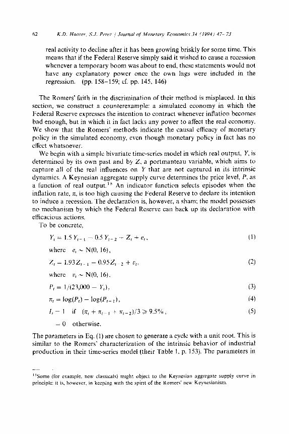
real activity to decline after it has been growing briskly for some time. This means that if the Federal Reserve simply said it wished to cause a recession whenever a temporary boom was about to end, these statements would not have any explanatory power once the own lags were included in the regression. (pp. 158-159; cf. pp. 145, 146)

The Romers’ faith in the discrimination of their method is misplaced. In this section, we construct a counterexample: a simulated economy in which the Federal Reserve expresses the intention to contract whenever inflation becomes bad enough, but in which it in fact lacks any power to affect the real economy. We show that the Romers’ methods indicate the causal efficacy of monetary policy in the simulated economy, even though monetary policy in fact has no effect whatsoever.

We begin with a simple bivariate time-series model in which real output, Y, is determined by its own past and by Z, a portmanteau variable, which aims to capture all of the real influences on Y that are not captured in its intrinsic dynamics. A Keynesian aggregate supply curve determines the price level, P, as a function of real output. l5 An indicator function selects episodes when the inflation rate, n, is too high causing the Federal Reserve to declare its intention to induce a recession. The declaration is, however, a sham; the model possesses no mechanism by which the Federal Reserve can back up its declaration with efficacious actions.

To be concrete,

Y,= 1.5Y,_, -0.5Y,_2+Z,fe,,

where e, N N(O, 16),

z, = 1.93Z,_1 - 0.95z,_, + U,,

where L+ - N(0, 16),

P, = l/(23,000 - Y,),

% = log(P,) - log(P,- 11,

I, = 1 if (n, + n,_, + 7r_2)/3 2 9.5%,

= 0 otherwise.

(1)

(2)

(3)

(4)

(5)

The parameters in Eq. (1) are chosen to generate a cycle with a unit root. This is similar to the Romers’ characterization of the intrinsic behavior of industrial production in their time-series model (their Table 1, p. 153). The parameters in

‘“Some (for example. new classicals) might object to the Keynesian aggregate supply curve in

principle; it is, however, in keeping with the spirit of the Romers’ new Keynesianism.

K.D. Hoover, S.J. Perez I Journal of‘ Monetary Economics 34 (1994) 47- 73 63

Eq. (2) are chosen to generate a damped cycle, with a periodicity of about four years, taking the unit of observation to be a month. The variable 2 is meant to reflect influences on real output that are themselves cyclical independently of output. Replacement investment cycles are an example of what Z might aim to capture. The critical thing is that Z is strictly exogenous for Y.16 Eq. (3) is a rectangular hyperbola with an asymptote representing the technical upper bound for output at 23,000; it is a textbook Keynesian reverse-l aggreg- ate-supply curve. Eq. (4) defines the rate of inflation. As Y cycles, P moves up and down the nonlinear aggregate supply curve, and rc varies. Eq. (5) selects times when the Federal Reserve declares its intention to fight inflation: if the three-month moving average of inflation is greater than 9.5 percent, I, takes a value of unity, indicating that the Federal Reserve wishes to combat inflation by inducing a recession. Notice that I, is recursively ordered after all of the other variables of the model: it does not affect them in any way. That is precisely the sense in which monetary policy has no real effects in this model. One cannot treat Z, for example, as a monetary shock, because there is no link between the Federal Reserve’s intentions and Z.

We use Eqs. (l)-(5) to generate an artificial time-series for Y, and I, indexed monthly January 1945 to December 1987. We choose initial values for Y,,,, rgb5, Y Feb. IgaS = 20,000 and for ZJan. rgh5, ZFeb. 1945 = 0, and we draw the error terms, e, and v,, from a random-number generator. The parameterization of the model is arbitrary, but this does not matter to the point at hand, which is whether the Romers’ methods are efficacious in general; logically, any counter- example would prove the point.

Having generated at artificial time-series for Y, we then apply the exact method used by the Romers for industrial production. We consider as monetary shocks four dates (February 1946, January 1954, February 1974, and January 1984) at which I, = 1. Fig. 5, showing the plot of the cumulated errors for January 1974, is typical of the dynamic simulations using these dates. They are remarkably similar to the Romers’ own simulations. On average, after thirty-six months the cumulative forecast error for simulated output is about 16 percent. Fig. 6 presents the impulse response function for simulated output. A unit shock to monetary policy would appear to cause a 26 percent fall in simulated output after thirty-six months. Comparing a regression of simulated output on a con- stant and seasonal dummies to one that adds the current value and thirty-six lagged values of the four monetary shock dummies shows that the monetary shock dummies reduced the residual variance of the regression by 18 percent. These results are summarized in Table 5. The results for the simulated data are

“See Engle et al. (1983) for a discussion of strict exogeneity. Strict exogeneity is closely related to the

absence of Granger-causality from Y to Z. Given that we are discussing a nonequivalent sense of

causality, it is best to avoid the potentially confusing term ‘Granger-causality’ wherever possible.

64 K.D. Homer, S.J. Perrz / Jm~ul qf Monerary Economics 34 (l994j 47-- 73

-25 ! _ , _p.^-

1974.02 1974.08 1975.02 1975.08 1976.c%? 1976.08 Dote

Fig. 5. Cumulative forecast errors from univariate time-series model for simulated data after the

January 1974 monetary shock. Univariate time-series model regresses the first difference of the

logarithm of monthly, simulated data on twenty-four own lags and monthly dummies. Data

construction described in text.

of precisely the same character as those of the Romers. We cannot, however, claim that they provide evidence for the causal efficacy of monetary policy; for in our model, monetary policy has no influence whatsoever.

The Romers’ method is not capable of distinguishing the case in which monetary policy is efficacious from the case in which it is not. The Romers claim that times in which the Federal Reserve intends to induce a recession are probably exogenous interventions. But is this likely? As they say, intentions must be realized in actions. We could modify Eq. (2) to render monetary policy efficacious:

-5 = @,jZ,- 1. z,-2, I,), @,<O. (2’)

Now when the Federal Reserve thinks inflation is too high, they clamp down on monetary policy in a way that affects output. But, of course, in this modified model, the decision to fight inflation is not exogenous; it is not independent of events in the real economy. On reflection, this is clearly as it should be. The Romers appear to believe that monetary policy can have reaI effects. This possibility is summarized in the nonvertical aggregate supply curve. A world with such a supply curve is one in which changes in prices are related to changes in output. When the Federal Reserve is reacting to high inflation, it is also reacting to cyclically high output; its reaction and its subsequent policy actions are endogenous in precisely the sense that the Romers wished to deny.

K.D Hoover, S.J. Perez I Journal qf’ Monetary Economics 34 (1994) 47- 73 65

-25

0 2 4 6 8 10 12 14 16 18 20 22 24 26 28 30 32 34 3t Months after Shock

Fig. 6. Impulse response function for simulated data. Time-series model regresses the first difference

of the logarithm of monthly, seasonally unadjusted industrial production on twenty-four own lags,

monthly dummies, and the current value and thirty-six lags of a dummy that takes the value I at the

date of a shock and 0 elsewhere. The cumulated effect of a unit shock to the dummy variable is

plotted. Data construction described in text.

Table 5

Some summary statistics of the simulated model

Average ocerpredictions qf the dynamic simulations after

the monetary shock dates

Maximum

After 36 months

Impulse response to a unit shock to the monetary dumm?

Maximum

After 36 months

Percentage of cariance explained by the monetary dummies

19%

16%

- 27%

- 23%

18%

Data are simulated according to the model described in Eqs. (l)-(5) in the text for a nominal period

January 1945 to December 1987. The simulation identified four monetary shocks: February 1946,

January 1954, February 1974, and January 1984. Statistics are calculated in the same manner

as the analogous statistics from Tables 1, 2, and 4; see the notes to those tables for further details.

The features of our model that subvert the Romers’ methods are very general. Without specifying much underlying detail our particular structure nests most Keynesian models. But the point goes beyond Keynesian models. A method based on a univariate model connected to some sort of indicator function, as Y, is connected to I,, is likely to fail in much the same way as the Romers’ method

66 K.D. Hoover, S.J. Perez / Journal qf Monetary Economics 34 (1994) 47- 73

does, so long as there exists a strictly exogenous influence on the variable of interest. Hamilton (1983), for example, shows that oil prices are strictly exogenous for GNP. While there are no doubt other candidates for Z, this is comforting empirical evidence that Z is not an empty box.

5. Dynamic forecasting is not the right technique, anyway

The Romers use dynamic forecasts from a univariate model for the plausible reason that they want to perform a counterfactual experiment; they want to see what would have happened to industrial production or unemployment in the absence of the monetary shock. Essentially, the Romers are using dynamic forecasts as a specification test: is monetary policy an omitted variable?

To construct a forecast, one first estimates a regression over a sample period (in this case 1945-1987). The estimated coefficients are then treated as param- eters to predict Y, recursively, for each t in the sample. Such forecasts use past values of Y, twenty-four of them in the Romers’ regressions. If the actual values of Y, _ i are used, the forecast is called ‘static’. If the previously predicted values of Y,-i are used, the forecast is called ‘dynamic’. A static forecast clearly corrects for errors induced by unpredicted shocks or noise. The apparent appeal of the dynamic forecast is that, in using only past forecasts, information about the noise is not introduced, so they indicate what would have happened in the absence of the noise.

In this section, we argue that dynamic forecasts are not useful specification tests. The argument is detailed, but its structure is simple. First, we show that dynamic forecasts contain the identical information to static forecasts. Dynamic forecasts could, therefore, provide a better specification test only if they presented that information in a more perspicuous form. We then argue that, in fact, dynamic forecasts present that information in a fundamentally muddled form. In particular, common estimation procedures determine some of the properties of dynamic forecasts independently of any facts about the real world.

The detailed development of our argument largely follows Pagan (1989). Pagan’s analysis is very general; it is nonetheless easily illustrated using a simple example. Consider a single-equation AR (1) process:

Y,=cpY,-, +ax,+ u,, t=l,2 ,..., T. (6)

The ordinary (static) residuals from a regression estimating the coefficients of Eq. (6) are

US= yt-cp*y,_i-or*x,, (7)

where (p* and z* are estimates of cp and CI. For most of the commcn estimators (OLS, 2SLS, 3SLS, etc.), 1 U,” = 0 by construction. The static forecasts of Y, are

K.D. Hoover, S.J. Perez / Journal qf Monetary Economics 34 (1994j 47- 73 61

given by

Y; = cp*Y,_l + fX*x,. (8)

The dynamic forecasts and dynamic forecast errors are defined recursively by

Yp = cp*yp_1 + c(*x,, Y,” = Y,, up= Y,- up.

(i) Dynamic forecasts contain the identical information to static forecasts.

Subtracting Eq. (9) from Eq. (8) yields

Y,” - Yp = cp*(Y,_r - Yp-,) (10)

or

(Y,- YP,+(YS- Y,)=cp*(Y,-,- YE,); (10’)

therefore

up = @UP_, + up. (11)

After repeatedly lagging Eq. (11) and substituting for the dynamic forecast error on the right-hand side, we obtain for cp* < 1

(11’)

Eq. (11’) states that the dynamic-forecast errors can be expressed as the weighted sums of current and past static forecast errors ~ i.e., there is no information contained in the dynamic forecasts not already available in the static forecasts. Hence, if static forecasts should not be used in counterfactual argument, because one cannot distinguish between the effects of omitted yet relevant variables (like monetary shocks) and other sources of noise, neither should dynamic forecasts. Unless, of course, the dynamic forecasts somehow present that same informa- tion more clearly. We believe that this is far from true.

(ii) Dynamic,forecasts present information relative to omitted variables in afin-

damentally muddled form. Even though the informational content of dynamic and static forecasts is identical, dynamic forecast errors compound the effect of the omitted variable with the cumulated effects of every other source of residual error, ‘. . so that it is harder to know whether a particular pattern to the [Up]

is due to genuine specification error or to colored noise’ (Pagan, 1989, p. 133).”

“The Ye’ do not correspond exactly to the dynamic forecasts used by the Romers. The F are the

dynamicf forecasts that take the first twenty-four actual values for industrial production and unemployment as initial values [the analogues to YO in Eq. (9)]. To generate their dynamic forecasts,

the Romers take the actual values at the date of the monetary shock and the immediately preceding

twenty-three periods as initial values. In the AR(l) example, it is easily shown that the errors when

68 K.D. Hoover, S.J. Perez 1 Journal qf‘A4onelar.v Economics 34 (19941 47- 73

Furthermore, as we now show, some of the properties of the dynamic forecast are artifacts of the estimation procedure and reveal nothing about real data or the causal structure of the real world.

As we noted above, ordinary regression residuals must sum to zero. This places restrictions on the dynamic forecast errors. To develop this theme somewhat further, sum up Eq. (11):

which can be rewritten as

(12’)

since

T

cU$=O and U,“=O.

Eq. (12’) shows that the dynamic forecast errors are not independent of each other. Indeed, this lack of independence, induced by the estimation procedure, is seen starkly when Eq. (6) has a unit root (i.e., when CJJ = 1) ~ as the corresponding equation for industrial production does for the Romers. In that case, Eq. (12’) implies that IJ,” = 0; that is to say that the dynamic forecast ‘. . . is ‘back on track’ at the end of the simulation period regardless ofthe adequacy ofthe model, but this is merely an artifact of the estimation procedure, and clearly can reveal nothing whatever about the quality of the model’ (Pagan, 1989, p. 132).18

one initializes at the date of the shock, Uy, are related to those when one initializes at the beginning

of the sample, Up, as

for t > k + 1, where k is the date of the shock. Everything concluded about the Up is also true

mutatis mutandis of the UP”: the ‘colored noise’ merely takes on a slightly different hue.

‘*The Romers (p. 153, Table I) estimate their industrial production regression in first differences of

logarithms, and then plot the cumulated dynamic forecast errors. Their regression thus contains by construction an exact unit root for the level of industrial production. The sum of coefficients on the

lagged levels of the unemployment rate in their unemployment rate regression (p. 156, Table 2) is 0.9716, which is high, but not quite a unit root. That Pagan’s result holds is easily confirmed by

plotting the cumulated dynamic forecast errors for industrial production. These drift about con-

siderably, but nevertheless return to zero at the end of the sample. Because unemployment does not

have an exact unit root, a plot of the dynamic forecast errors for unemployment comes close to but does not quite return to zero at the end of the sample.

K.D. Hoover. S.J. Perez / Journal of Monetary Economics 34 11994) 97- 73 69

Our analysis has proceeded so far in terms of a simple, single-equation, AR( 1) example. It is easily generalized to systems of equations

Y,= Y,_i@-t Y,B+X,A+ u,, (13)

where bold type indicates vectors or matrices. Since any AR(x) process can be rewritten as an AR( 1) process with auxiliary equations, the results generalize in that way as well. The analogue for cp = 1 - i.e., a unit root in Eq. (6) ~ is that @ possesses a unit eigenvalue. As we noted earlier, this is the case for the Romers’ equation for industrial production, and nearly so for their equation for unemployment.

One might be tempted to conclude that, because part of the problem with dynamic forecasts arises from constraints imposed by estimating the regression coefficients using the complete sample, forecasts using recursive or rolling regressions might provide a suitable alternative method of specification testing. The problem is to discriminate between misforecasts arising from omitted monetary-shock variables and other sources of misspecification. Unfortunately, rolling regressions in themselves provide us neither a method for discrimination nor a metric of misspecification. Formal specification tests in either nested or nonnested frameworks generally require the explicit specification of alternative relevant factors. The exclusion tests reported in Section 3 above can be inter- preted in a nested or encompassing framework (Hendry, 1987; IIendry and Richard, 1987). Table 4 shows that a regression for industrial production includ- ing oil dummies clearly encompasses one that also includes monetary dummies: i.e., monetary dummies may be, but oil dummies oil dummies as regressors without significant loss of information.”

In summary: dynamic forecasts are a poor way of checking for the existence of an omitted variable, such as monetary policy shocks, and they are misleading guides to the quantitative effects of such shocks. More appropriate specification tests do not support the Romers’ conclusions about the efficacy of monetary policy. It is important to note once again, however, that our investigation is narrow, so that one can fairly reach only a negative conclusion about the adequacy of the Romers’ evidence, and not a positive conclusion about an alternative causal explanation of business cycles.

6. The problem is with the statistics, not with the narrative approach

The Romers’ narrative/statistical approach fails to provide adequate evidence of causal efficacy. The problem, however, is not with the narrative, but with the

“This conclusion is keeping with the general thrust of Boschen and Mills (1988) that suggests that real variables in general have explanatory power for real output, whereas various monetary

variables do not.

70 K.D. Hoover, S.J. Perez 1 Journal of Monetary Economics 34 11994) 47- 73

statistics and with the failure to use the narrative effectively to illuminate the statistics and the statistics to illuminate the narrative. Whatever the pitfalls and ambiguities of interpreting the narrative record ~ and, as the Romers observe, they are real and many - the Romers’ method of connecting the narrative with statistical information is startlingly simple. If causal inference were really so simple, it is surprising that the method was not discovered and widely applied long ago. To offer a positive alternative and to shed further light on why the Romers’ technique is bound to be unsuccessful, we sketch a method of causal inference in which narrative and statistics more effectively illuminate one another.

The central fact about causation is that it is asymmetric. If A causes B, it is a special case if B also causes A. Regressions are themselves asymmetric, but it has long been known that regressions do not come marked with the true causal direction: how do we know that the regression of A on B is causally correct (i.e., B causes A), while the regression of B on A is not? If we stick to statistics alone, the answer is: ‘we don’t’. This is where a narrative approach, properly deployed, can help.

Hoover (1990) develops an alternative methodology of causal inference. We give a brief, and necessarily incomplete, sketch of the main ideas here. Following Simon (19.53) causality is characterized in the true (unobservable) data-generat- ing process as an asymmetrical relation of recursion. For example, in Eqs. (l)-(5), one would say that Z, causes Y,, which in turn causes rcr, which causes I,. Any such system of equations can be represented as a joint probability distribu- tion. Considering only Y and Z, we can write this D( Y, Z). Unfortunately, even though causal direction may be well-defined in the data-generating process, the joint distribution cannot reveal it on its own.

Consider the two ways in which we can factor the joint distribution into the product of a conditional and a marginal distribution,

D(Y,Z)=D(YIZ)D(Z)=D(ZlY)D(Y). (14)

The two conditional distributions and the two marginal distributions can be thought of, at least in the context of normality, as regression equations, and therefore as reflecting asymmetry. The middle pair can be thought of as Z caus- ing Y, while the right-hand pair would be Y causing Z. The famous problem of observational equivalence is simply that when there is no variation in the underlying data-generating process, the two pairs are statistically identical (Basmann, 1965, 1988; Sargent, 1976). There is no choosing between them.

Suppose, however, that historical narration can provide instances in which the underlying Y process changes and other instances in which the underlying Z process changes. Suppose that the (unknown) truth is that Y causes Z. With some caveats, it can be shown that an intervention to the underlying Z process will produce a structural break in the regressions representing D(Z 1 Y) and D(Z) as well as D( Y 1 Z). That there are structural breaks in both the marginal and the

K.D. Hoover. S.J. Perez / Journal qf Monetary Economics 34 (1994) 47- 73 71

conditional distributions for Z provides a check that the break indicated by the narrative is truly in the Z process. That the regression of the conditional distribution of Y has a structural break is the consequence of the mismatch between the direction of conditionalization in the regression and the causal direction of the true underlying causal order. D(Y) would remain invariant to such an intervention; this is one of the hallmarks of the true causal order. Similarly, it can be shown that an intervention to the underlying Y process will produce structural breaks in regressions corresponding to both D( Y ]Z) and D(Y). A regression corresponding to D(Z) will also break down, the asymmet- ries again conflict. The regression corresponding to D(Z ( Y) will remain invari- ant. The intuition is that, when Y causes Z, the actual value of Y carries all the necessary information for Z independently of what factors determine the value of Y. This invariance is the second hallmark of the true causal order. Of course, if Z truly caused Yin the true underlying data-generating process, then their roles would be reversed in the above invariance relations. Thus, combining a narra- tive approach with a statistical approach designed to reveal the fundamental causal asymmetry has the potential to support empirical causal inference (see Hoover, 1991, and Hoover and Sheffrin, 1992, for applications).20

The alternative causal methodology is only sketched here (details, caveats, and reservations are found in Hoover, 1990, 1991). Even the bare bones of this alternative shed some light on the difficulties of the Romers’ methodology.

First, the Romers’ method uses single equations. Unlike, the alternative factorings of the joint probability distribution, these provide no statistical check on causal asymmetries.

Second, it is not clear that the Romers have used their narrative approach to identify events that truly qualify as inventions in the underlying data-generating process. Such an intervention must alter deep structure. What the Romers choose to call monetary shocks are times when the Federal Reserve has said that it wished to reduce output to reduce inflation. The Federal Reserve could very well be following a stable reaction function, such as Eq. (5) and make such announcements. The deep structure of the data-generating process would then be constant, observational equivalence would reign, and there would be no basis for causal discrimination. Examples of interventions that would be potentially structural are changes in the policy rule or changes in the regulatory environ- ment (e.g., permitting a financial innovation in the banking system).

The third point is related to the first two: the Romers provide no statistical confirmation that their shocks are truly monetary shocks. In Section 3 above, we

“It is interesting to note that Friedman and Schwartz (1963a, p. 215) cite the invariance of the money/income relationship across great changes in monetary institutions as important evidence on

the direction of influence between money and income. They do not, however, exploit the asymmetry

of regressions to systematically explore invariance with respect to different classes of interventions.

72 K.D. Hoover, S.J. Perez / Journal qf’bfonetary Economics 34 11994) 47- 73

saw that the data conform as easily to oil shocks as to the Romers’ monetary shocks. In the alternative methodology, the narrative may suggest that a mone- tary shock occurs. Before one would believe it, however, one would expect to find the characteristic sign of structural breaks in both conditional and marginal regressions for money. The only support the Romers provide for there having been a shock is the Federal Reserve’s expression of an intention to contract, and the only support they provide for causal asymmetry is that this intention seems to be followed by a contraction. But this is reasoning post hoc ergo propter hoc;

and the well-known fallacy brings us full circle.

7. Conclusion

The Romers have rightly stressed the importance of coordinating narrative information about history and institutions with statistical information in draw- ing causal inferences. Unfortunately, the way in which they attempt to coordi- nate this information can shed no light on causal questions. While we applaud the use of a narrative approach, we have questioned the validity of the Romers’ methodology on three fronts. It is important to realize that each front is independent of the others. If any one of the three is sustainable, the Romers’ method cannot be an efficacious causal methodology.

First, the identification of economic shocks may not be unique. We showed that oil shocks had the same explanatory power, conditional on the validity of the rest of the Romers’ method, as their monetary shocks. We do not make a case for the importance of oil shocks; we merely point out that the Romers have not made a better case for monetary shocks.

Second, the Romers’ method cannot distinguish between cases in which monetary policy is causally efficacious and cases in which no actions whatsoever follow Federal Reserve expressions of intention to tighten policy. Using simulated data in which monetary policy was ineffective by construction and, again, using the Romers’ own methods, we were able to generate results of a similar character to their own. Their method simply does not discriminate.

Third, the method of dynamic forecasting is inappropriate to the problem at hand. There is no information in dynamic forecasts that is not also in ordinary regression residuals. The Romers use dynamic forecasts to test whether monet- ary policy is an omitted variable in a time-series regression. Dynamic forecasting does not provide a theoretically valid basis for such a test.

We take no position here with respect to the truth about the question: Does money matter? Our argument is methodological. The Romers’ methodology ignores the central problem of causal inference, which is: What evidence is needed to determine the nature of causal asymmetries in a world that, statistically speaking, may be characterized by observational equivalence? Money may matter or money may not matter; but there is nothing in the Romers’ evidence for the postwar period that should convince an open-minded observer one way or the other.

References

Basmann, R.L., 1965, A note on the testability of ‘explicit causal chains’ against the class of

‘interdependent’ models, Journal of the American Statistical Association 60, 1080-1093.

Basmann, R.L., 1988, Causality tests and observationally equivalent representations of econometric

models, Journal of Econometrics 39, 699101.

Blanchard, Qlivier, 1990, Why does money affect output: A survey, in: Benjamin M. Friedman and

Frank H. Hahn, eds., Handbook of monetary economics, Vol. 2 (North-Holland, Amsterdam).

Boschen, John F. and Leonard 0. Mills, 1988, Tests of the relation between money and output in the

real business cycle model, Journal of Monetary Economics 22, 3555374.

Engle, Robert E., David F. Hendry, and Jean-Francois Richard, Exogeneity, Econometrica 51,

113-127.

Friedman, Benjamin M., 1990, Comments and discussion [on Romer and Romer (1990)], Brookings

Papers on Economic Activity, no. I, 204209. Friedman, Milton, 1970, Comment on Tobin, Quarterly Journal of Economics 82, 318-327.

Friedman, Milton and Anna J. Schwartz, 1963a, A monetary history of the United States, 1867-1960

(Princeton University Press, Princeton, NJ).

Friedman, Milton and Anna J. Schwartz, 196313, Money and business cycles, Review of Economics

and Statistics 45; reprinted in: Milton Friedman, The optimum quantity of money and other

essays (Aldine, Chicago, IL).

Hamilton, James D.. 1983, Oil and the macroeconomy since World War Ii, Journal of Political

Economy 91,228-248.

Hammond, J. Daniel, 1992, Interview with Milton Friedman, in: Research in the history of economic

thought and methodology, Vol. 10, forthcoming.

Hendry, David F., 1987, Econometric methodology: A personal perspective, in: Truman F. Bewley,

ed., Advances in econometrics, Vol. 2 (Cambridge University Press, Cambridge).

Hendry, David F. and Jean-Francois Richard, 1987. Recent developments in the theory of en-

compassing, in: B. Cornet and H. Tulkens. eds., Contributions to operations research and

econometrics: The XXth anniversary of CORE (MIT Press, Cambridge, MA).

Hoover, Kevin D., 1990, The logic of causal inference: Econometrics and the conditional analysis of

causation, Economics and Philosophy 6, 2077234.

Hoover, Kevin D., 1991, The causal direction between money and prices: An alternative approach,

Journal of Monetary Economics 27, 381-423.

Hoover, Kevin D. and Steven M. Sheffrin, 1992, Causation, spending and taxes: Sand in the sandbox

or tax collector for the welfare state?, American Economic Review 82, 225-248.

Pagan, Adrian, 1989, On the role of simulation in the statistical evaluation of econometric models,

Journal of Econometrics 40, 125-139.

Romer, Christina D. and David H. Romer, 1989, Does monetary policy matter? A new test in the

spirit of Friedman and Schwartz, in: Olivier Blanchard and Stanley Fischer, eds., NBER

macroeconomics annual, Vol. 4 (MIT Press, Cambridge, MA). Romer, Christina D. and David H. Romer, 1990, New evidence on the monetary transmission

mechanism, Brookings Papers on Economic Activity, no. I, 149-198.

Sargent, Thomas J., 1976, The observational equivalence of natural and unnatural rate theories of

macroeconomics, Journal of Political Economy 84; reprinted in: Robert E. Lucas, Jr. and

Thomas J. Sargent, eds., 1981, Rational expectations and econometric practice (George Allen

and Unwin, London) 5533562.

Simon, Herbert A., 1953, Causal ordering and identifiability, Ch. 1 in: Herbert A. Simon, 1957, Models of man (Wiley, New York, NY).

Tobin, James, 1970, Money and income: Post hoc ergo propter hoc?, Quarterly Journal of

Economics 82. 301&317.