1

8th Ottawa Group Meeting - Helsinki - 23-25 August 2004

Comparison of Variance Estimators for the Consumer Price Index Anders Norberg, Statistics Sweden

Anders Norberg, Dept. of Economic Statistics, Statistics Sweden, Box 24300, S-104 51 Stockholm, Sweden

anders.norberg@scb.se Abstract Estimates of sampling errors are of importance for survey designers when allocating sample sizes, in production as a tool for output editing and for users of statistics in decision making. The use of two-dimensional designs with elements of non-probability sampling methods, annually updated samples and complex estimators creates problems when estima-ting sampling variances for CPI-statistics. In this paper the character of variation in price changes is studied by use of analysis of variance models with one locality and one item effect and an error corresponding to the selection of product offers. This yields valuable information for the sample allocation work. Variance estimators in analytical forms, expressed in schemes of resampling procedures and model based formulas are tested in a large simulation study. A random groups method is proposed. This method makes it possible to estimate the variance for complex functions of index links such as e.g. the annual change of quarterly average inflation rates. .

1 Introduction Measures of statistical errors for statistics have many uses: to inform on the quality for users of the statistics, to produce a basis for a better allocation of resources in production and to detect possible serious errors in the data when output editing. The study in question here was initiated to meet the needs of the former of the above-mentioned objectives for the users of the Swedish Consumer Price Index, KPI. One of the three methodology approaches that were tried are, however, particularly appropriate for resource allocation. Dalén and Ohlsson (1995) worked out a variance expression for the KPI's short-term index link in the daily necessities system. They also put forward a proposal for an estimator for the variance. The daily necessities system is a "real" two-dimensional sample. Here we have one probability sample of outlets selling daily necessities and three samples of representative items, one for each of the three outlet chains that have a dominant market share in trade in daily necessities in Sweden. Representative items are, however, often exactly specified products. For goods and services other than daily necessities, the price collector makes a choice out of the products available within a more or less broad definition of the representative item. The person collecting the prices also decides which replacement products should be chosen when they are forced to find a replacement product. This person should also make an evaluation on the quality of the products. On a micro level, "changes in price" can therefore occur when replacement products are chosen. The choice of products offered, including quality evalua-

2

tions, may influence the index and its variance more than the choice of outlet or representative item. This has not been sufficiently investigated in Sweden. It could even be that the price collector�s selection is significant for the index and variation in data. We can expect the variance estimator suggested by Dalén and Ohlsson (1995) to overestimate variance if it is applied to the sample dimensions outlets and representative items, and if the variance between products is large in comparison to the variance between the representative items. In this paper, a further number of proposals for variance estimators are given. Simulations have been carried out to assess and compare them. These simulations have been carried out partly on completely synthetic populations and partly on populations taken from KPI data. Bases, formulae and calculation systems in Sweden's consumer price index today are described in section 2. Section 3 gives details of eight variance estimators. The results of the simulations with these estimators are reported in section 4. Certain applications and results are presented in section 5. The conclusions of the study, with recommendations for methods, are given in section 6.

2 General principles and methodology of the Swedish KPI today

The basic principle The 1943 Index Commission (SOU, 1943) undertook a review of the foundations of the index. The idea that, as a matter of principle, the index should refer to the same standard of living in two different time periods was explicitly outlined. The method of calculating the index, still termed the �Cost of Living Index�, was revised. From then on, it was computed as a chained index with annual links, in which the weights apply to the current year. The basic link in the index is defined as the price change between two successive Decembers, with quantity weights representing the whole calendar year between them. Longer-term comparisons could be obtained by multiplying successive links together into a chained index.

The chained index today The current index base year is 1980. For each successive new link, weights are recalculated based on new information. We make a distinction between this long-term link (L), which uses quantity weights Qy from year y and the short-term link (K), which uses quantity weights Qy-1 from year y-1. The definitions of the links are

�

�−− =

k

yk

12,1yk

k

yk

12,yk

12,y12,1y QP

QPL (1)

and

�

�−−

−

− =

k

1yk

12,1yk

k

1yk

m,yk

m,y12,1y QP

QPK , (2)

3

where summation is over N products with subscripts k (subscripts will later be dropped when there is no risk for misunderstanding). The chained index from base year 0 to month m in year Y will now be1:

m,Y12,1Y

12,1Y12,2Y

12,y12,1y

12,112,0

12,00

m,Y0 KL...L...LIKPI −

−−− ⋅⋅⋅⋅⋅⋅= (3)

12-month changes When 12-month changes are published, the long-term index component is replaced by the corresponding short-term component instead of looking at the changes in the index series according to (3) directly. One reason for this procedure is that the long-term component includes substitution effects that do not represent the current 12-month period and another reason is the need for international comparability. The price change from Y-1,m to Y,m is thus calculated as:

== −−

−−−−

mYY

YY

mYY

mYmY KKKKPI ,1

12,212,112,2

,12,1

,,1 12,1Y

12,2Y

12,1Y12,2Y

m,1Y0

m,Y0

LK

KPIKPI

−−

−−

− (4)

The 12-month changes according to (5) are often used for monitoring inflation. For example, the inflation target of the Swedish Riksbank (the central bank) is the moving average of twelve 12-month changes according to (5).

Index aggregation at the higher level The National Accounts provide value weights, V, at the higher KPI aggregation levels. These are defined as "price times quantity", in our notation, V=P*Q. Up-to-date National Accounts consumption values today exist for more than 100 consumption categories. During the annual weight revision, which takes place in January and early February, new National Accounts values are brought into the index. Below the level where National Accounts weights are available, it is necessary to vary procedures. Household Budget Surveys (HBS) are used for breaking down many NA categories into smaller groups. For food, Statistics Sweden aggre-gates scanner data received from the three leading chains in the retail market.

Index aggregation at lower levels At the lowest level, elementary aggregation, the KPI generally uses the RA formula in the sense of Dalén (1992).

�

�

+

+= −−

−

−

k

m,yk

12,1yk

12,1ykk

k

y,mk

12,1yk

m,ykk

m,y12,1y )pp/(pw

)pp/(pwI (5)

1 The extra link from 0 to 0.12 is needed in order to use a full year as the index reference period. Its exact definition is: � −−=

m

m,012,112

112,012,1

12,00 KLI

4

The motivation for the RA formula is partly that it can be seen as an approximation of the basic formula (2). The RA formula can also be shown to approximate a geometric mean index quite well.

New index construction In the Swedish KPI publication for January 2005 and onwards, the KPI numbers will be com-puted by using an improved index construction. Like now, the KPI will also subsequently be computed as a chain index with annual links. In the new construction the annual link will measure how much the average price level in the year concerned has changed from the ave-rage price level of the preceding year. The CPI basket of the annual link will reflect a blend of consumption patterns of the year concerned and the preceding year, according to a Walsh-formulae. The new index construction will also make it possible to use more data from the national accounts and to use them more accurately for the index weights. A further change is that sub-indices on the lowest levels of aggregation will be computed as geometric means of price relatives.

Central and local price collection There are basically two different modes of price collection. For most services and some goods, the central staff collects the prices, either by telephone or using a small-scale postal survey with shuttle forms, and enters them directly into the computer, usually into an Excel Workbook, where the sub-index computation is done. This procedure is usually referred to as central price collection. For many goods and services, there is local price collection. The specifications for so called representative items are established centrally. In some cases, the specifications are broad and the price collectors can select the "most sold" product (a product offer) within the specifica-tion in a selected outlet. In other cases, the specifications are tight and the price collectors pick corresponding products in the sampled outlet or, if one is not found, omit the product. Prices are collected by price collectors by visiting the outlets directly or by a telephone call. The price collectors are located all over Sweden and are employed on a full- or part-time basis as interviewers for all surveys managed by the Statistics Sweden. The collection process takes place on an optional day in the week in which the 15th of the month occurs. In each outlet, from one up to as many as 500 prices are observed. In all, some 25 000 prices in 900 outlets are observed in the local price collection. Prices are entered into forms, which are later scanned; for clothing and PCs, shuttle forms are used. Before product-group price indices are calculated, data are checked for significant deviations compared with last month�s price. They are corrected if errors are discovered, contacts with price collectors being made where necessary. When all sub-indices have been finalized in their preliminary versions, a general meeting of the KPI staff is held where output editing is performed.

5

Sampling methods in local price collection Sampling of representative items in the daily necessities system For foodstuffs (except for fresh food, such as meat and vegetables) and other daily necessities, product sampling is carried out by Pareto π ps (see Rosén(2000)), using sampling frames provided by the three major retail chains in Sweden. These are estimated to be some 80% of all goods sold in supermarkets. The sampling frame covers products at a detailed level, where a unique price normally exists, for example � EAN = 7331040056126 Coca Cola Light, plastic bottle, 1.5 litre�. Three different product samples of 400 items each are created, one for each of three major outlet chains. The product sample is then matched to the outlet sample according to the chain to which a sampled outlet belongs. Only products offered in the sampled outlet are thus inclu-ded. This reduces the effective product sample size in each outlet to some 250-300 products offered. There are 40 supermarkets and 9 hypermarkets in the outlet sample. Sampling of representative items in clothing and other local prices systems For clothing, furniture, other goods sold in the retail trade and services, such as restaurants, the representative items are chosen and specified judgmentally, in a manner typical for consumer price index methods in most countries. Outlet sampling in local price collection In product groups, where local price collection is used, outlets are divided into 50 retail trade and service strata according to SNI code (Swedish Standard Industrial Classification, which closely follows NACE, Rev. 1, the EU standard). In each stratum, a sample of outlets is drawn from the Business Register by an order π ps technique. This first gross sample is drawn about 6 months before the year in which the sample is to be used. This sample is then screened, in October/November, both in the central office and by the price collectors visiting the outlets, and some of the outlets initially drawn are excluded for various reasons. For example, they may be head offices rather than outlets, or they may not sell any of the sampled products. In the case of clothing, a purposive allocation of representative items to the sampled outlets takes place. A sample design with overlapping panels is implemented by the use of random numbers permanently associated with every outlet in the sampling frame. Sampling rotation is performed so that 20% of the random numbers are changed every year. Combined with changes in the sampling frames, this results in some 70-75% of outlets remaining in the sample from one year to the next. See Ohlsson (1990 and 1995) or Statistics Sweden (2001) for a description of this technique.

New and disappearing products and outlets / replacements New samples are introduced when a new index link is started up in December, when both the old and the new product and outlet samples are measured. In this way, an overlap is created, so that the old sample is used for back comparisons and the new sample for forward compa-risons, without any explicit quality adjustment. To the extent that the market is in equilibrium, so that the price differentials between the old and the new sample in December reflect genuine

6

consumer valuation of quality differences, and that both samples adequately represent the population of product offers, the estimator of price changes is unbiased. For clothing and footwear, the former requirement is not fulfilled and an adjustment for obsolescence of the old sample is made. Where an outlet remains in the sample from one year to the next, the sampled products offers are normally not exchanged in December. The replacement of a particular product offer with another in the same outlet is caused by the disappearance or reduced significance of a product offer. In this case, a quality adjustment is normally done. Outlets are not replaced during the year. New outlets are only introduced in the course of updating samples in December, in connection with the start-up of a new link. In those, very few, cases where an outlet is closed down or price measurements cease to be possible for some other reason, that outlet�s products offers are deleted.

Quality change Quality adjustment in the clothing system The rapid changes of items in the clothing market make advanced and complex methods for dealing with replacements and quality adjustments necessary. For this reason, hedonic models of the relationship between clothing prices and characteristics are formulated and estimated. The adjustment for obsolescence is also significant. Due to the needs of the hedonic model method, data collection and processing is more expensive than for other product areas. Quality adjustment for other products in the local price collection Here, the price collectors perform the adjustments. By quality difference is understood a difference in function, comfort, durability, security, guarantees and easiness of handling etc.. Differences in quality are to be valued from the viewpoint of the consumer. The price collec-tor should try to assess how the average consumer experiences differences in material and design. This is difficult and in practice it means that he/she will have to use his/her own assessment of the differences. Quality adjustments according to these principles are difficult to make. The quality adjustment is measured as how much better or worse the new variety is, in money terms. Non-quality adjustment products in local price collection For products where quality adjustments are not made, but package size has been altered, only new package sizes where the quantity change is less than 50% are accepted as replacements. A proportional adjustment is then made so that the price effectively becomes a price per quantity unit. In other cases, where a product offer can no longer be found, it is deleted and the price change is imputed from the rest of the products offered in the product group.

7

3 Variance estimation methods

Variance is a statistical measure of variation for a random variable. When, as is the case here, the random variable is an affected measurement of a studied phenomenon (in this case, inflation) we can interpret the variance as a measure of statistical uncertainty. The uncertainty we are analysing here is due to the fact that inflation is calculated using a sample of outlets, items and product offers - it is not possible to collect data on all transactions in society. The variance we are trying to estimate here is only one component of the statistical uncertain-ty which occurs because of the sample. There are other sources of errors in statistics, which can be considered more serious. In Dalén (1999), sources for the bias and size of these errors are assessed. One assumption for the concepts of variance and variance estimating is that we, in principle, have statistical samples, i.e. samples that have been selected using random methods and with known probability. This assumption is fulfilled with regard to the outlet sample and the product sample in the daily necessities system. For clothes and other locally priced items, we must compromise with the principles and consider the sample of items and/or products offers as random. We can either see them as:

a) A random sample of representative items in the first stage and the collection of the "most sold" products offered within the representative items, which would not mean a choice, in the second stage, neither deliberate nor random.

b) A random sample of representative items in the first stage and a random (at least arbitrary) sample of product offers in a second stage, independently drawn in each outlet.

c) A stratification of the markets by the representative items, which therefore covers all or a large part of the market, and a random (arbitrary) sample of product offers in one single stage, independent between outlets.

The first alternative imitates the real two-dimensional statistical sample, which is used in the daily necessities system.

Taylor linearisation Dalén and Ohlsson (1995) have derived variance expressions for index based on a two-dimensional sample and suggest an estimation of the variance. Such variances and variance estimators have three terms that can be interpreted as variance between products, between outlets and an interaction term. Definition:

gm is the number of products in the sample, in product groups g

hn is the number of outlets in the sample, in outlet groups h

ghv is the weighting, based on sales during one year, for the combination (g, h). The

weighting is standardized so that �� =G

g

H

hgh 1v .

8

Rgiπ and C

hjπ are sample probabilities for product offer i within commodity group g and outlet j within outlet group h. Define the RA term on a micro level:

���

=otherwise0

11ij

joutlet in available isoffer product if

2/)( 10

00

ijij

ijij pp

pf

+=

2/)( 10

11

ijij

ijij pp

pf

+= (6)

For each i, Riw is a weighting for product offer i and for each j, C

jw is a weighting for outlet j. These weightings depend on the size (turnover) of the particular sample object and sample procedure (OSU, PPS, etc.) The weighting is standardized so that ��

∈∈

==Ch

Rg Uj

Cj

Ui

Ri ww 1 for

each g and h.

Let 01�

ijCj

Ui

Ri

Ujijgh fwwX

Rg

Ch

� �∈ ∈

= , 1ij

Cj

Ui

Ri

Ujijgh fww1Y�

Rg

Ch

� �∈ ∈

= (7)

0� =ghX where product i is not traded in outlet j, the same applies to ghY�

gh

ghgh X

YI �

�� =

is a "cell index". (8)

The KPI's short-term index link becomes ��=G

g

H

hghghIvI �� (9)

Previously � �∈ ∈

==−=Rg

ChSi Sj

ghij

h

ghij

gijghijij

ghij e

ne

mfIfe �1e� ,�1e� ),�(1� gh

.jghi.

01 (10)

Dalén and Ohlsson suggest, after some the following variance estimator for I� .

INTBUTPROO&D V�V�V�V� ++= (11)

( )2

h

gh.i

gh

gh

Si

Rgi

g ggPRO e�

X�v

1)1m(m

1V�Rg ��

���

��

���

−−

= ���∈

π (12)

( )2

g

ghj.

gh

gh

Sj

Chj

h hhBUT e�

X�v

1)1n(n

1V�Ch ��

���

��

���

−−

= ���∈

π (13)

( )( )( )��

���

��

���

−−−−⋅−−

= ����∈ ∈R

gChSi Sj

2ghj.

gh.i

ghij

Rgi

Chj

g h gghh2gh

2gh

INT e�e�e�11)1m(m

1)1n(n

1X�v

V� ππ (14)

9

Standard formulae for one- and two-stage OSU Under the assumption that the setting of prices in a market, say retail trade of furniture, is not decided by one outlet changing their price strategy or by the price for one type of furniture (a representative item) changing overall, it could be a reasonable approximation to consider the collected data as generated by a simple random sample, SRS, from the whole population of products offers in the country. Variance estimators according to standard formulae for stratified SRS in one stage from the whole market, with regard to finite sampling corrections, is a reference method. Two-stage sampling, with stratified SRS of outlets in the first stage and independent stratified SRS of products offers per outlet, and vice versa, is an interesting and easily calculated alternative.

Replication techniques A number of techniques based on replication have been suggested for variance estimation in the last 50 years. Unbiased and dependent random groups, balanced half-samples, the jackknife and the bootstrap are well-known examples (Wolter (1985)). In certain situations, one or more of them are not suitable. In the case of the KPI, there are some considerations to be made:

• There are many strata, both in the outlet and in the product dimension. The sample size in some outlet strata is as small as 6 and, in the product dimension, only one representative item.

• Some sample units, outlets as well as representative items, are selected with certainty and some are selected with high inclusion probabilities, while most sample units are selected with small inclusion probabilities.

• The samples are updated once a year. We require a variance estimating procedure that, in the best possible way, measures the effect of rotating outlet samples, the introduction of new goods and services and new item weights on sampling variance.

We propose a repetitive use of the dependent random groups method with the minimum number of random groups, k=2, in each repetition.

Repeated random groups (1)

We have an estimator Y� based on a sample. We create k sub-samples, each with 1/k of the sample object, in best manner so that the design of each sub-sample is the same as the full sample regarding stratification, rotation, etc. We create the estimator αY� . An estimator of the

variance of Y� is ( )2Y�Y�

1k1

α−−

. This estimation has only one degree of freedom. We prefer to

use all αY� and calculate

( ) ( )� −−

=α

α2

Y�Y�1k

1k1Y�V� . (20)

10

Let us choose k = 2. We thus make a sub-sample of half of all data and create the estimator

½�Y . An estimator of the variance for Y� is ( )2

½�� YY − . This estimator has only one degree of

freedom but we estimate the variance many times by repeatedly drawing "half samples" and take the mean value of estimated variance to ensure sufficient quality in the final variance estimator. Up to this point, we have used established theories. How can a good variance estimator be produced when we meet a two-dimensional sample? The following procedure is a trial, which has been tested in a simulation study. Let us draw a "half sample", i.e. create a random group with k=2, in both dimensions so that, as a result, we only include a quarter of all data. Study the following random breakdown of a total sample in two dimensions:

x11 x12

x21 x22

Let x11, x12, x21 and x22 be four figures, which can correspond to the sums of a variable for the same number of objects in the four boxes. With a little algebra, we get the following:

=−⋅�� ��= = = =

2

1r

2

1c

2

1r

22

1crcrc )xx4(

41

( ) +−+⋅= � ��= = =

2

1r

2

1r

22

1crc2r1r )xxx2(

21

( )� ��= = =

+−+⋅+2

1c

2

1r

22

1crcc2c1 )xxx2(

21

( ) ( ) ��

���

� −+⋅+−+⋅+ ����= == =

2

1r

22

1crc2112

2

1r

22

1crc2211 )xxx2()xxx2(

21 (15)

We can call these three terms between-outlet, between-items and interaction squared totals, and hopefully they will correspond to the variance components (12) - (14). The finite population corrections for certain large sample probabilities can be significant. The use of explicit corrections such as ( )π−1 is impractical, particularly as the sample probability for an outlet, for example, is different from year to year. π is the inclusion probability and ( )π−1 is therefore the finite correction factor. Let us test the following procedure: We are looking for the individual value of k (�number of random groups�, which no longer need to be a whole number) per sampled object (outlet and product) which is such that

( )1

11−

⋅−k

π is equal to 1.

11

In this way, the effect of the finite population correction is included in the procedure to select a replica of the sample. We choose to set this statement to 1 because it corresponds to a half sample (k=2), without a finite sampling correction factor, and we get a simple calculation formula. A little algebra leads to the "half sample" probabilities

)2/(1p ii π−= (16)

that are in the range 0.5 � 1.0. Because we now select slightly over half of all outlets and items/products in a "half sample", it is in practice appropriate to select only one of the four "half samples", say the one based on the box r=1 and c=1. With Q repetitions of the procedure, we get the variance estimator

( ) ( )� −=Q

q

2q11)1(RG Y�Y�

Q1Y�V� (17)

Random groups estimation with two-stage sampling (2) and (3) According to Wolter (1985), page 31, when selecting a multi-stage sample, random groups should be created by, in a random way, dividing the sample of primary selected units, PSU, into k groups, while keeping the original sample design as much as possible. All samples in later stages should remain undivided. Also, since finite population corrections are not used, variances may be underestimated. We measure variable Y in a two-dimensional population. The measurement value is yij for the i th sample unit in the first dimension and the j th sample unit in the second dimension. Let iY� be an estimator of iY based on any design with a probability sample of second-stage units. An estimator of a total Y from a simple random sample of n PSUs, with the replacement from a population with N is

�=

⋅=n

1iiY�

nNY� (18)

The usual variance estimator is according to Des Raj's (1968) "Sampling Theory"

2b

22n

1i

n

1iii

2

1 sn

NY�n1Y�

1n1

nN)Y�(V� ⋅=�

�

���

� −⋅−

⋅= � �= =

(19)

where 2n

1i

n

1iiiii

2b yM

n1yM

1n1s � �

= =

��

���

� −⋅−

=

The usual variance estimator for the HT-estimator of a total Y from a SRS without replacement of n PSUs from a population with N and SRS without the replacement of mi second-stage units from Mi is

�=

���

����

�−⋅+⋅�

�

���

� −⋅=n

1i

2wi

ii

2i

2b

2

2 sM1

m1M

nNs

Nn1

nN)Y�(V� (20)

where ( )2m

1jiij

i

2wi

i

yy1m

1s �=

−⋅−

=

12

From these estimators, Jönrup (1974) has formulated an underestimation and overestimation of the variance for SRS without replacement. Underestimation is obtained by (20) when only the first term is retained. Overestimation is obtained by (19) because an SRS sample with replacement gives a greater variance than a sample without replacement with the same sample sizes. So,

2b

2

22b

2

sn

N)Y�(V�sNn1

nN ⋅<<⋅�

�

���

� −⋅ (21)

applies. When the sample fraction Nn is very small, the contribution from "within PSU term"

will also be small and the variance can be estimated only by an analysis of the variation bet-ween estimators of totals of PSUs. This is equivalent to sub-sampling PSUs, when using the random groups method or similar. In the KPI, we do not want to disregard finite sampling corrections, which occur both in the outlet and items dimensions because, in many cases, they are zero or close to zero. For example, there has not been any doubt that bananas should be included in the KPI. When estimating variance as if the sample were a two-stage sample and observing the finite population corrections, we consequently get underestimations. Variance analysis shows that price changes in many markets happen in an apparently random manner; they cannot be explained by the effects of either the outlets or the items themselves. Let us assume that we have a two-stage sample from a two-dimensional population with NM objects in which the measurement values yij have been generated as random figures, i=1,...,N and j=1,...,M. On "average" therefore, all 2

wis are the same and can be taken as the mean of the measurement values for all first-stage units according to the following:

( ) 2w

22m

j

n

1ii

n

1iij

22m

jiij

2wi sny

n1y

n1

1m1n�yy

1m1s ⋅=�

�

���

� −−

⋅=−−

= � ���==

(22)

We can now formulate the following variance estimator:

( ) ��

���

�⋅⋅�

�

�

� −⋅⋅+⋅��

�

� −⋅⋅

= 2w

22

2b

2

223 snMm1

mM

nNs

Nn1

nN

MN1Y�V�

2w

2b s

Mm1

m1

Nns

Nn1

n1 ⋅�

�

���

� −⋅⋅+⋅��

���

� −⋅= (23)

where 2n

1i

n

1iii

2b y

n1y

1n1s � �

= =

��

���

� −⋅−

=

From a random groups design with a total variance that is the sum of the between-outlets, between-products and interaction variances, we form a variance estimator consisting of the

13

between-outlets variance plus the sampling fraction for the outlet sample (n/N) multiplied by the between-products variance, or vice versa2.

( ) ( ) ( )�=

++ ��

���

� −+−=Q

1q

22212

21211)2(RG Y�Y�

NnY�Y�

Q1Y�V� (24)

We convert this variance estimator into one single procedure for repeated random half samp-ling. We have already chosen a "half sample" of outlets/items with the probabilities

)2/(1p )1()1( π−= and all items/outlets, under the assumptions we have made here,

Nn

)( =1π . We introduce Mm

)( =2π for the second-stage sample. Now we would also

select a "half sample" of items/outlets so that ( )1k

11 )2()1( −⋅−⋅ ππ becomes 1, which means

that the items should be selected with the proportion

( ))2()1()2( 11

1k1p

ππ −⋅+== . (25)

We see that if 11 =)(π , we should select second-stage units within the PSUs in the same way as we have selected the PSUs when 11 <)(π . The estimator based on Q replications is

( ) ( )� −=Q

q

2q11)3(RG Y�Y�

Q1Y�V� (26)

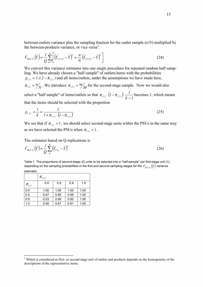
Table 1 The proportions of second-stage (2) units to be selected into a �half-sample� per first-stage unit (1), depending on the sampling probabilities in the first and second sampling stages for the ( )Y�V� )3(RG variance

estimator

)( 2π

)( 1π 0.0 0.5 0.9 1.0

0.0 1.00 1.00 1.00 1.00 0.5 0.67 0.80 0.95 1.00 0.9 0.53 0.69 0.92 1.00 1.0 0.50 0.67 0.91 1.00

2 Which is considered as first- or second-stage unit of outlets and products depends on the homogeneity of the descriptions of the representative items.

14

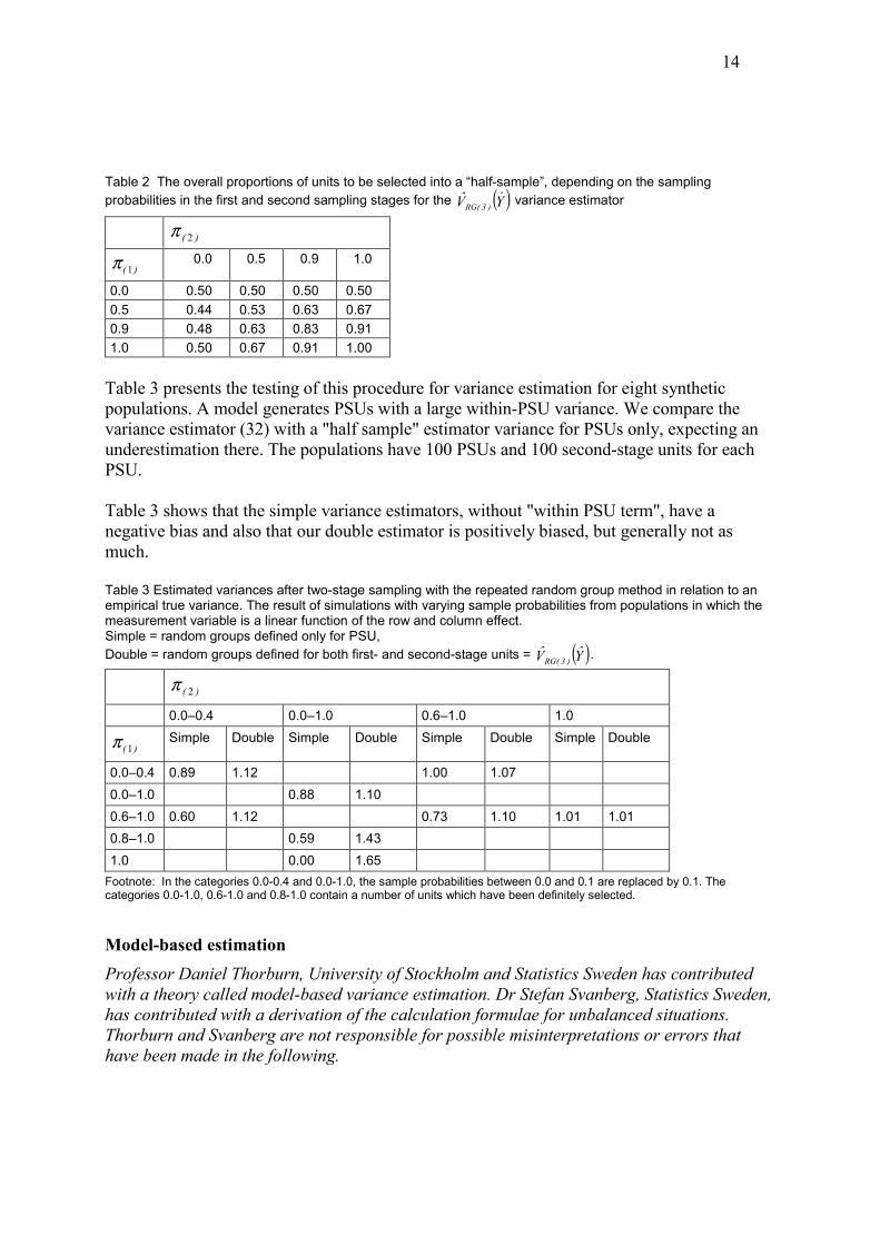
Table 2 The overall proportions of units to be selected into a �half-sample�, depending on the sampling probabilities in the first and second sampling stages for the ( )Y�V� )3(RG variance estimator

)( 2π

)( 1π 0.0 0.5 0.9 1.0

0.0 0.50 0.50 0.50 0.50 0.5 0.44 0.53 0.63 0.67 0.9 0.48 0.63 0.83 0.91 1.0 0.50 0.67 0.91 1.00

Table 3 presents the testing of this procedure for variance estimation for eight synthetic populations. A model generates PSUs with a large within-PSU variance. We compare the variance estimator (32) with a "half sample" estimator variance for PSUs only, expecting an underestimation there. The populations have 100 PSUs and 100 second-stage units for each PSU. Table 3 shows that the simple variance estimators, without "within PSU term", have a negative bias and also that our double estimator is positively biased, but generally not as much. Table 3 Estimated variances after two-stage sampling with the repeated random group method in relation to an empirical true variance. The result of simulations with varying sample probabilities from populations in which the measurement variable is a linear function of the row and column effect. Simple = random groups defined only for PSU, Double = random groups defined for both first- and second-stage units = ( )Y�V� )3(RG .

)( 2π

0.0�0.4 0.0�1.0 0.6�1.0 1.0

)( 1π Simple Double Simple Double Simple Double Simple Double

0.0�0.4 0.89 1.12 1.00 1.07 0.0�1.0 0.88 1.10 0.6�1.0 0.60 1.12 0.73 1.10 1.01 1.01 0.8�1.0 0.59 1.43 1.0 0.00 1.65

Footnote: In the categories 0.0-0.4 and 0.0-1.0, the sample probabilities between 0.0 and 0.1 are replaced by 0.1. The categories 0.0-1.0, 0.6-1.0 and 0.8-1.0 contain a number of units which have been definitely selected.

Model-based estimation Professor Daniel Thorburn, University of Stockholm and Statistics Sweden has contributed with a theory called model-based variance estimation. Dr Stefan Svanberg, Statistics Sweden, has contributed with a derivation of the calculation formulae for unbalanced situations. Thorburn and Svanberg are not responsible for possible misinterpretations or errors that have been made in the following.

15

Suppose that prices for all products offers are set according to a stochastic procedure with four random number generators. Let =ijkY the logarithm of price changes (December of year y-1 to month m of year y). We assume that observations are generated according to

ijkijjiijkY ε+δ+γ+β+µ= , (27)

where ijhg rknjmi ,..,1,,..,1,,..,1 ===

µ is a general mean value without variance

iβ is a representative item effect

jγ is an outlet effect

ijδ is an interaction effect between representative items and outlets

ijkε is a product offer effect

Assume that iβ is normally distributed with the expected value 0 and variance 2βσ , that jγ is

normally distributed with the expected value 0 and variance 2γσ , that ijδ is normally

distributed with the expected value 0 and variance 2δσ and finally that ijkε is normally

distributed with the expected value 0 and variance 2εσ . In this case, ijkY is normally distributed

with variance 2222εδγβ σ+σ+σ+σ .

Assume that we have a sample. Let: Y�=Σijk Yijk

Yi..=Σjk Yijk

Y.j.=Σik Yijk

Y..k=Σij Yijk

Yij.=Σk Yijk When carrying out a variance analysis, the squared sum is divided

��� −= 2...ijkY )YY(SS into two parts:

The variation which is explained by the factors

����= ===

+−−+−+−g hhg m

1i

2....j.

n

1j..i.ij

n

1j

2....j.

m

1i

2.....i )YYYY()YY()YY( (28)

and the part which cannot be explained, the so-called residual squared sum:

���= = =

−=g h ijm

1i

n

1j

2...

r

1kijk )YY(SSE (29)

16

The SAS system has a procedure for analysis of variance with random effect, which allows a varying number of observations per cell, ijr . The result provides the basis for the calculation

of estimates of 2� βσ , 2�γσ , 2�εσ and 2� εσ

procprocprocproc glmglmglmglm data=pop; class outlet item; model pkvot=outlet item outlet*item; random outlet item outlet*item;; runrunrunrun; quit;

When we have these estimators, we can also estimate variances for the mean values of logarithmic price ratios for a sample of representative items ( gm ), outlets ( hn ) and total number of products offered ( ijp ), at least if the sample of products offered is fairly similar in size for all representative items and outlets. As long as we can generate data for a process, we get:

=+++=

=+++=

=+++=

=+++=

�������

������ �� �

������������

������

= = == ===

= = == == == =

= = == = == = == = =

= = == = =

)(V)r(V)r(V)r(V

)(V)r(V)r(V)r(V

)(V)(V)(V)(V

))((V)Y(V

g h ijg hhg

g h ijg hh gg h

g h ijg h ijg h ijg h ij

g h ijg h ij

m

1i

n

1j

r

1kijk

m

1i

n

1jijij

n

1jj.j

m

1i.ii

m

1i

n

1j

r

1kijk

m

1i

n

1jijij

n

1j

m

1iijj

m

1i

n

1jiji

m

1i

n

1j

r

1kijk

m

1i

n

1j

r

1kij

m

1i

n

1j

r

1kj

m

1i

n

1j

r

1ki

m

1i

n

1jijk

r

1kijji

m

1i

n

1j

r

1kijk

εδγβ

εδγβ

εδγβ

εδγβ

������= == ===

+++=g hg hgg m

1i

n

1jij

2m

1i

n

1j

2ij

2m

1i

2j.

2m

1i

2.i

2 rrrr εδγβ σσσσ (30)

When we take a sample from a finite population of outlets, representative items and product offers, we should be able to use the following estimator of variance.

Let the total number of observations be ����=== =

===hgg h n

1jj.

m

1i.i

m

1i

n

1jij rrrr

Our variance estimator for KPI data is

222

m

1i

2j.

hg

hg

22

m

1i

2j.

h

h22

m

1i

2.i

g

g

i j kijk

�r1

Rr1�

r

r

NMnm

1

�r

r

Nn1�

r

r

Mm

1Yr1V�

g

gg

εδ

γβ

σσ

σσ

⋅⋅��

���

� −+⋅⋅��

�

�

��

�

�

⋅⋅

−+

+⋅⋅���

����

�−+⋅⋅

��

�

�

��

�

�−=�

�

�

�

�

��� � �

=

==

(31)

17

4 Simulations

The proposed variance estimators have been tested on a number of finite populations of outlets, representative items and products. We have created completely synthetic populations and populations with data from the samples that we have in the KPI database. We have only one product stratum (g) and one outlet stratum (h). We consider stratum not to be a problem in this context. From each population, we have drawn thousands of two-dimensional samples with SRS in both dimensions. We consider varying sampling probabilities not to cause any special problem compared to sampling with equal probabilities. The samples are often large in relation to the populations (about 50 %) so that it has been necessary to pay attention to the finite population corrections. In tests with clothing and furniture data, we have chosen two products offered per combina-tion of representative item (i) and outlet (j). The price index link has been calculated with the Swedish RA-formula in one step for the whole sample, as in the KPI.

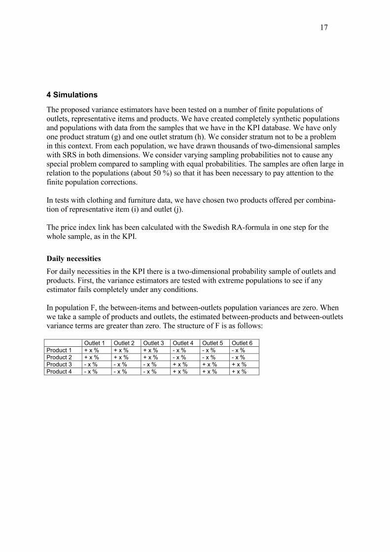
Daily necessities For daily necessities in the KPI there is a two-dimensional probability sample of outlets and products. First, the variance estimators are tested with extreme populations to see if any estimator fails completely under any conditions. In population F, the between-items and between-outlets population variances are zero. When we take a sample of products and outlets, the estimated between-products and between-outlets variance terms are greater than zero. The structure of F is as follows: Outlet 1 Outlet 2 Outlet 3 Outlet 4 Outlet 5 Outlet 6 Product 1 + x % + x % + x % - x % - x % - x % Product 2 + x % + x % + x % - x % - x % - x % Product 3 - x % - x % - x % + x % + x % + x % Product 4 - x % - x % - x % + x % + x % + x %

18

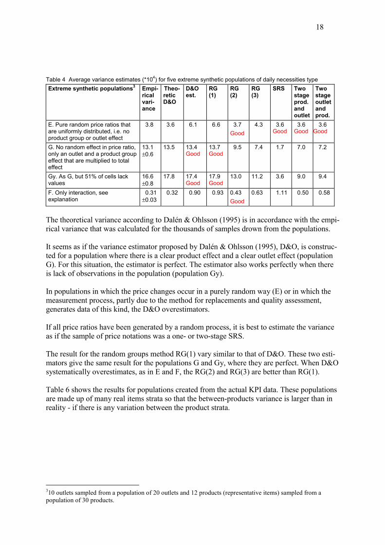
Table 4 Average variance estimates (*104) for five extreme synthetic populations of daily necessities type Extreme synthetic populations3 Empi-

rical vari-ance

Theo-retic D&O

D&O est.

RG (1)

RG (2)

RG (3)

SRS Two stage prod. and outlet

Two stage outlet and prod.

E. Pure random price ratios that are uniformly distributed, i.e. no product group or outlet effect

3.8 3.6 6.1 6.6 3.7 Good

4.3 3.6 Good

3.6 Good

3.6 Good

G. No random effect in price ratio, only an outlet and a product group effect that are multiplied to total effect

13.1 ±0.6

13.5 13.4 Good

13.7 Good

9.5 7.4 1.7 7.0 7.2

Gy. As G, but 51% of cells lack values

16.6 ±0.8

17.8 17.4 Good

17.9 Good

13.0 11.2 3.6 9.0 9.4

F. Only interaction, see explanation

0.31 ±0.03

0.32 0.90 0.93 0.43 Good

0.63 1.11 0.50

0.58

The theoretical variance according to Dalén & Ohlsson (1995) is in accordance with the empi-rical variance that was calculated for the thousands of samples drown from the populations. It seems as if the variance estimator proposed by Dalén & Ohlsson (1995), D&O, is construc-ted for a population where there is a clear product effect and a clear outlet effect (population G). For this situation, the estimator is perfect. The estimator also works perfectly when there is lack of observations in the population (population Gy). In populations in which the price changes occur in a purely random way (E) or in which the measurement process, partly due to the method for replacements and quality assessment, generates data of this kind, the D&O overestimators. If all price ratios have been generated by a random process, it is best to estimate the variance as if the sample of price notations was a one- or two-stage SRS. The result for the random groups method RG(1) vary similar to that of D&O. These two esti-mators give the same result for the populations G and Gy, where they are perfect. When D&O systematically overestimates, as in E and F, the RG(2) and RG(3) are better than RG(1). Table 6 shows the results for populations created from the actual KPI data. These populations are made up of many real items strata so that the between-products variance is larger than in reality - if there is any variation between the product strata.

310 outlets sampled from a population of 20 outlets and 12 products (representative items) sampled from a population of 30 products.

19

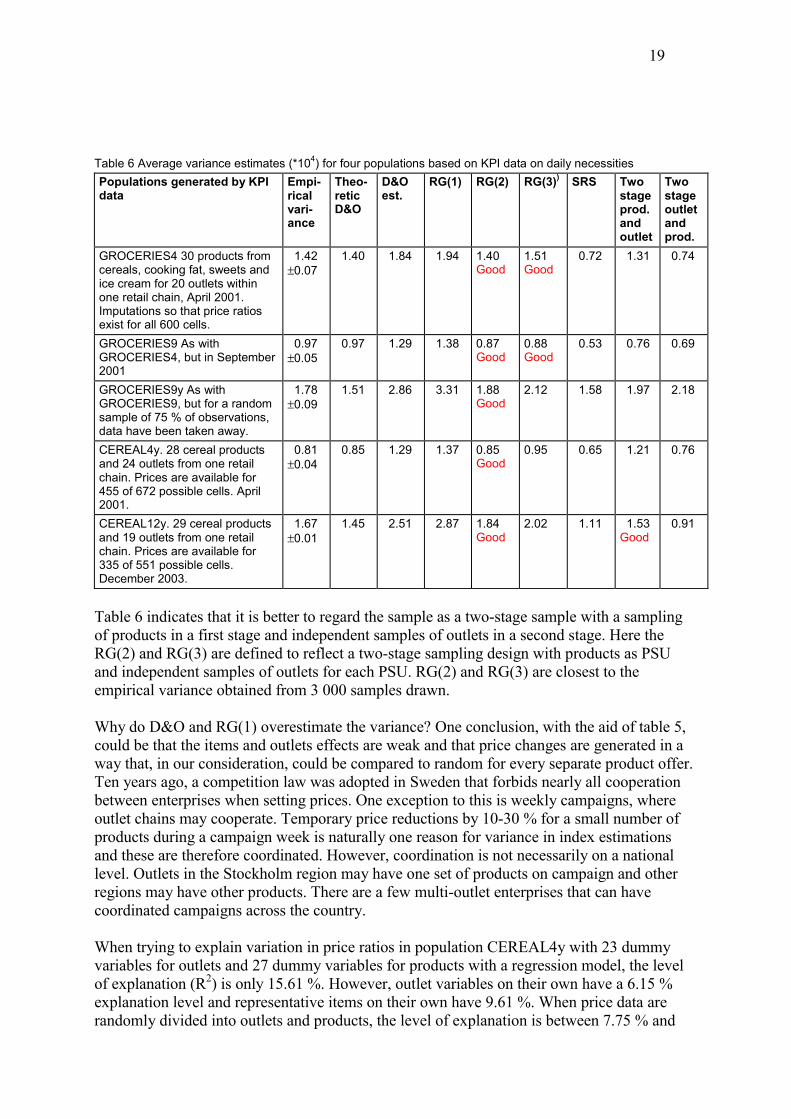
Table 6 Average variance estimates (*104) for four populations based on KPI data on daily necessities Populations generated by KPI data

Empi-rical vari-ance

Theo-retic D&O

D&O est.

RG(1) RG(2) RG(3)) SRS Two stage prod. and outlet

Two stage outlet and prod.

GROCERIES4 30 products from cereals, cooking fat, sweets and ice cream for 20 outlets within one retail chain, April 2001. Imputations so that price ratios exist for all 600 cells.

1.42 ±0.07

1.40 1.84 1.94 1.40 Good

1.51 Good

0.72 1.31 0.74

GROCERIES9 As with GROCERIES4, but in September 2001

0.97 ±0.05

0.97 1.29 1.38 0.87 Good

0.88 Good

0.53

0.76 0.69

GROCERIES9y As with GROCERIES9, but for a random sample of 75 % of observations, data have been taken away.

1.78 ±0.09

1.51 2.86 3.31 1.88 Good

2.12 1.58

1.97 2.18

CEREAL4y. 28 cereal products and 24 outlets from one retail chain. Prices are available for 455 of 672 possible cells. April 2001.

0.81 ±0.04

0.85 1.29 1.37 0.85 Good

0.95 0.65

1.21 0.76

CEREAL12y. 29 cereal products and 19 outlets from one retail chain. Prices are available for 335 of 551 possible cells. December 2003.

1.67 ±0.01

1.45 2.51 2.87 1.84 Good

2.02 1.11 1.53 Good

0.91

Table 6 indicates that it is better to regard the sample as a two-stage sample with a sampling of products in a first stage and independent samples of outlets in a second stage. Here the RG(2) and RG(3) are defined to reflect a two-stage sampling design with products as PSU and independent samples of outlets for each PSU. RG(2) and RG(3) are closest to the empirical variance obtained from 3 000 samples drawn. Why do D&O and RG(1) overestimate the variance? One conclusion, with the aid of table 5, could be that the items and outlets effects are weak and that price changes are generated in a way that, in our consideration, could be compared to random for every separate product offer. Ten years ago, a competition law was adopted in Sweden that forbids nearly all cooperation between enterprises when setting prices. One exception to this is weekly campaigns, where outlet chains may cooperate. Temporary price reductions by 10-30 % for a small number of products during a campaign week is naturally one reason for variance in index estimations and these are therefore coordinated. However, coordination is not necessarily on a national level. Outlets in the Stockholm region may have one set of products on campaign and other regions may have other products. There are a few multi-outlet enterprises that can have coordinated campaigns across the country. When trying to explain variation in price ratios in population CEREAL4y with 23 dummy variables for outlets and 27 dummy variables for products with a regression model, the level of explanation (R2) is only 15.61 %. However, outlet variables on their own have a 6.15 % explanation level and representative items on their own have 9.61 %. When price data are randomly divided into outlets and products, the level of explanation is between 7.75 % and

20

14.65 % for 10 such random experiments. In the actual KPI data, coordinated variations bet-ween outlets or products are consequently hardly larger than for a completely random data. The estimators D&O and RG(1) give almost similar results. Correlation between these estimators are at least 0.97 for the four populations in table 6. The random groups method gives systematically higher estimates, which, at a guess, could depend on some form of rounding off effect, i.e. when the sub-sample is to be drawn from sample sizes that are not whole numbers. Because of the limited set of conditions for this study, there can very well be situations where for example one outlet or two in the sample suddenly changes the prices radically, depending on new ownership or the like. As the total sample size is about 50, this can cause a significant outlet effect and an underestimation of variance with the RG(2) and RG(3) estimators.

Clothing and other locally priced items Clothing and other locally priced items are characterised by the price collector selecting one or more products offered in each outlet for each representative item. In the measurement of clothing, the sample of products offers often consists of 3-5 pieces per outlet and representative item. Furniture is another example, where 2 products offers per outlets are sampled. This means that clothing and furniture are interesting to use as an illustration which will hopefully be applicable to statements about locally priced items in general. In the following simulations, a sample of outlets and representative items is first drawn. For every combination of outlet and representative item, 2 products offers are randomly selected with SRS. When the D&O variance estimator, the sizes of the population and sample of representative items are considered as doubled, i.e. the two selected products offers are considered as representative items. This is how Statistics Sweden works in the local price system. For example, a product offer for items chair A and chair B are selected according to the same specifications, so that several product offers will be obtained without the need to specify many different representative items.

21

Table 7 Average variance estimates (*104) for synthetic populations of clothing and furniture type Synthetic populations Empi-

rical vari-ance

D&O est.

RG(1) RG(2) RG(3) SRS Two stage prod. and outlet

Two stage outlet and prod.

Modelbased esti-ma-tion

E2A. Population of 20 outlets and 30 items4. Price ratio computed as sum of outlet-, item-, interaction-effects and error. Standard deviation for Outlets = Items = Interaction = Error = 1.0

0.076 0.063 0.084 Good

0.063 0.048 0.009 0.038 0.042 0.078Good

E2A:OIE. As with E2A but without the between-item variance.

0.063 0.068 Good

0.073 0.068 Good

0.070 Good

0.008 0.005 0.063 Good

0.071 Good

E2A:PIE. As with E2A but without the between-outlets variance.

0.042 0.027 0.047 Good

0.025 0.009 0.007 0.039 Good

0.005 0.043 Good

E2A:IE. As with E2A but without the between-outlets and between-items variance.

0.0079 0.0097 0.0128 0.0076 Good

0.0076 Good

0.0050 0.0050 0.0049 0.0081 Good

E2A:E. As with E2A but only with errors

0.0031 0.0042 0.0043 0.0026 0.0030 Good

0.0025 0.0017 0.0017 0.0032 Good

E2C. Populations as E2A with standard deviation similar to furniture data: Outlets=0.60, Items=1.11, Interaction=4.70 and Error=10.32.

0.79 1.06 1.25 0.70 0.73 Good

0.54 0.58 0.50 0.80 Good

E2B. Populations as E2A with standard deviation similar to clothing: Outlets=7.88, Items=4.79, Interaction=11.13 and Error=31.21.

5.9 7.2 8.3 5.4 5.6 Good

3.0 3.3 4.1 6.5 Good

E2By. As E2B, but with gaps for 50 % of the combinations outlet x item.

15.4 19.2 23.0 13.6 14.8 Good

9.1 12.5 13.0 16.3 Good

The model-based variance estimator is clearly the best. It is not completely perfect for data when there are gaps in the data. RG(3) is a random group method approximating a two-stage design variance when outlets are the PSU and products are the within PSU elements. We see that RG(3) estimator fails totally for population E2A:PIE where there is no outlet effect and RG(3) should not work.

4 10 outlets sampled from a population of 20 outlets and 15 representative items sampled from a population of 30 and finally 2 product offers from populations of 10 within each combination of outlet and item.

22

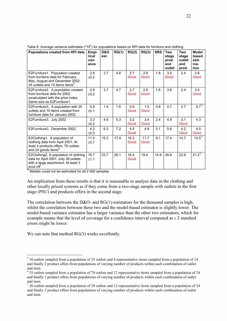
Table 8 Average variance estimates (*104) for populations based on KPI data for furniture and clothing Populations created from KPI data Empi-

rical vari-ance

D&O est.

RG(1) RG(2) RG(3) SRS Two stage prod. and outlet

Two stage outlet and prod.

Model based esti-ma-tion

E2Furniture1. Population created from furniture data for February, May, August and December 2002. 35 outlets and 14 items items5.

2.8 ±0.2

3.7 4.6 2.7 Good

2.9 Good

1.8 3.0 Good

2.4 2.8 Good

E2Furniture2. A population created from furniture data for 2002, recalculated with the price index. Same size as E2Furniture1.

2.8 ±0.2

3.7 4.7 2.7 Good

2.8 Good

1.8 3.8 2.4 3.0 Good

E2Furniture3. A population with 35 outlets and 10 items created from furniture data for January 2002.

0.9 ±0.1

1.4 1.6 0.9 Good

1.0 Good

0.8 0.7 0.7 0.7*)

E2Furniture3. July 2002 3.3 ±0.2

4.6 5.3 3.2 Good

3.4 Good

2.4 4.9 3.1 Good

4.3

E2Furniture3. December 2002. 4.2 ±0.3

6.3 7.2 4.5 Good

4.8 3.1 5.6 4.2 Good

4.5 Good

E2Clothing1. A population of clothing data from April 2001. At least 4 products offers. 76 outlets and 24 goods items6

11.0 ±0.7

15.3 17.4 10.3 Good

11.7 Good

9.1 17.4 14.7 13.5*)

E2Clothing2. A population of clothing data for April 2001, only 39 outlets with a large assortment. At least 3 prod off7

16.7 ±1.1

23.7 28.1 16.4 Good

19.4 14.9 26.8 23.9 21.2*)

*) Models could not be estimated for all 2 000 samples An implication from these results is that it is reasonable to analyse data in the clothing and other locally priced systems as if they come from a two-stage sample with outlets in the first stage (PSU) and products offers in the second stage. The correlation between the D&O- and RG(1)-estimators for the thousand samples is high, whilst the correlation between these two and the model-based estimator is slightly lower. The model-based variance estimator has a larger variance than the other two estimators, which for example means that the level of coverage for a confidence interval computed as ± 2 standard errors might be lower. We can note that method RG(3) works excellently.

5 10 outlets sampled from a population of 35 outlets and 8 representative items sampled from a population of 14 and finally 2 product offers from populations of varying number of products within each combination of outlet and item. 6 35 outlets sampled from a population of 70 outlets and 12 representative items sampled from a population of 24 and finally 2 product offers from populations of varying number of products within each combination of outlet and item. 7 20 outlets sampled from a population of 39 outlets and 12 representative items sampled from a population of 24 and finally 2 product offers from populations of varying number of products within each combination of outlet and item.

23

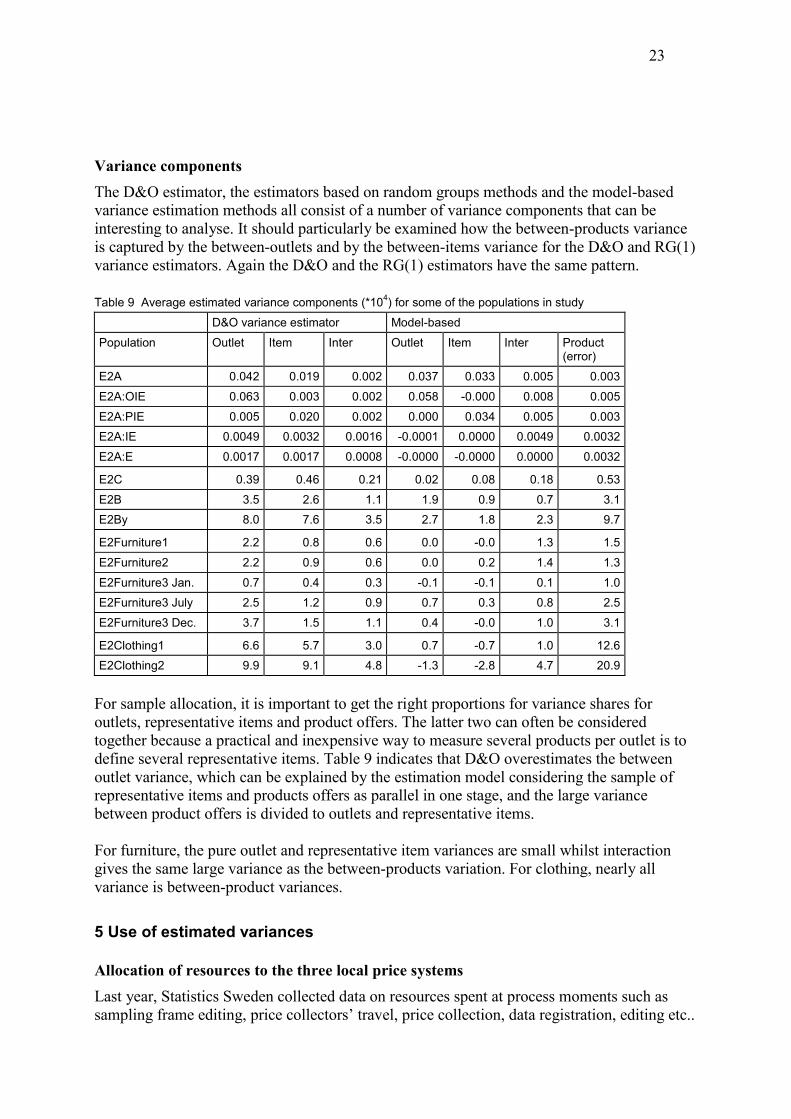
Variance components The D&O estimator, the estimators based on random groups methods and the model-based variance estimation methods all consist of a number of variance components that can be interesting to analyse. It should particularly be examined how the between-products variance is captured by the between-outlets and by the between-items variance for the D&O and RG(1) variance estimators. Again the D&O and the RG(1) estimators have the same pattern. Table 9 Average estimated variance components (*104) for some of the populations in study D&O variance estimator Model-based Population Outlet Item Inter Outlet Item Inter Product

(error) E2A 0.042 0.019 0.002 0.037 0.033 0.005 0.003 E2A:OIE 0.063 0.003 0.002 0.058 -0.000 0.008 0.005 E2A:PIE 0.005 0.020 0.002 0.000 0.034 0.005 0.003 E2A:IE 0.0049 0.0032 0.0016 -0.0001 0.0000 0.0049 0.0032 E2A:E 0.0017 0.0017 0.0008 -0.0000 -0.0000 0.0000 0.0032

E2C 0.39 0.46 0.21 0.02 0.08 0.18 0.53 E2B 3.5 2.6 1.1 1.9 0.9 0.7 3.1 E2By 8.0 7.6 3.5 2.7 1.8 2.3 9.7

E2Furniture1 2.2 0.8 0.6 0.0 -0.0 1.3 1.5 E2Furniture2 2.2 0.9 0.6 0.0 0.2 1.4 1.3 E2Furniture3 Jan. 0.7 0.4 0.3 -0.1 -0.1 0.1 1.0 E2Furniture3 July 2.5 1.2 0.9 0.7 0.3 0.8 2.5 E2Furniture3 Dec. 3.7 1.5 1.1 0.4 -0.0 1.0 3.1

E2Clothing1 6.6 5.7 3.0 0.7 -0.7 1.0 12.6 E2Clothing2 9.9 9.1 4.8 -1.3 -2.8 4.7 20.9

For sample allocation, it is important to get the right proportions for variance shares for outlets, representative items and product offers. The latter two can often be considered together because a practical and inexpensive way to measure several products per outlet is to define several representative items. Table 9 indicates that D&O overestimates the between outlet variance, which can be explained by the estimation model considering the sample of representative items and products offers as parallel in one stage, and the large variance between product offers is divided to outlets and representative items. For furniture, the pure outlet and representative item variances are small whilst interaction gives the same large variance as the between-products variation. For clothing, nearly all variance is between-product variances.

5 Use of estimated variances

Allocation of resources to the three local price systems Last year, Statistics Sweden collected data on resources spent at process moments such as sampling frame editing, price collectors� travel, price collection, data registration, editing etc..

24

In combination with estimated variances, an update of the total sample design is possible. These are the conditions, where the variances are estimated with method RG(3): Table 10 Weights, costs, estimated variances and best allocation for the three local price systems Daily

necessities Clothing Other locally

priced items KPI-weights 145.9 51.6 245.9 Variable costs8 (103 SEK) 1 102 1 523 3 716 Est. variance for inflation level without fpc9 0.037 3.02 0.089 Est. variance for monthly change of inflation with fpc 0.018 2.23 0.041 Optimal allocation of resources for estimating inflation level (103 SEK) 667 2 500 3 203 Optimal allocation of resources for estimating monthly change of inflation (103 SEK) 620 2 855 2 896 Assuming that we keep the design of each of the three sub-systems unchanged but are able to change the sample sizes proportionally to the resources spent on them, we can find the optimal allocation of resources by minimising a function of three variables under a cost restriction. We now find that the sample sizes should be increased for clothing. We can also see that, if there is a change in estimated inflation from one month to another, we would need an even larger sample for clothing than if we set the monthly change of inflation as the first priority. This can be explained by the rapid turnover of products and volatile price changes, which starts in January with the sales. The results in table 10 cannot be implemented fully because of the large number of retail trade industries covered by the �Other local prices system�. We need a minimum of outlets in the sample for each industry. Furthermore fresh fruits and fresh vegetables, included in the �Other local prices system�, cause a large variance contribution so the resources spent on price collection in supermarkets and hypermarkets should not be decreased to the extent showed in the table; from SEK 1 102 to 667 or � 40 %.

Allocation of resources within the three local price systems Table 7 indicates that the model based variance estimator works well. The analysis variance for clothing and furniture, also the analysis of daily necessities made, clearly show that the variance between outlets and the variance between representative items is small compared to the variance for product offers for an item in an outlet. Considering this and the fact that there is a large cost for price collector�s travels to and from the outlets leads to a design with few outlets and many products offers, possibly by many items, in each outlet. Therefore, Statistics Sweden have asked all the price collectors what is the maximum number of observations per outlets in all the retail trade industries, considering the working conditions, the attitudes of the personal and owners of the outlets. The analysis is made at present, hopefully leading to fewer outlets and mote observations in total.

8 Costs that are proportional to sample size 9 Finite population correction

25

Variance caused by a detailed structure of weighting classes in the KPI The elementary aggregates in KPI are defined by 287 product groups and 1�6 retail trade industries per group for the goods and services in this study. In all there are 761 combinations of these with a fixed CPI-weight. It is a difficult task to stratify the populations of outlets and products and to allocate the sample sizes optimally when the total index is a weighted sum of 761 elementary aggregates. With the �half-samples� defined by the RG(3)-method we have computed variance estimates under the model that there are no industry-effects, implying that all prices can be aggregated directly to the 287 items. This variance is 15 % smaller for the �Other local prices system�, where the number of industries is largest. For daily necessities the �reduction� of variances is 7 %, here there are only two industries. For clothing, where the variances are very large by nature, Statistics Sweden has, since 1990, applied the �model� that there are no significant differences between industries in price change; data from all industries are processed to produce item indices directly. The industry-weights are hopefully implicit approximately correct by the allocation of the samples

Technical bias in the long term index Estimates of ratios have a �technical� bias for most sampling designs. For the so called long-term link it is apparent why this bias exist. Remember that the long-term link for year y have product weights that are values of private consumption during the year y, which are backdated to the price reference period of the link, i.e. December year y-1. This back-dating means that the consumption values are divided by the average of price indices numbers for the twelve months January to December year y. Bear in mind that the index numbers are estimated, some of which with large sampling variances. If a product group happens to get a low price change for December and the whole year on average, the weight gets large by the backdating procedure and the low index gets too large a weight. Index numbers that are large by chance get low weights. The random sampling errors seems to cause a downward systematic error. This bias was estimated by Statistics Sweden 1996 on purely theoretical basis. Like the Jack-knife-method it is possible to estimate the bias with our RG(3) half-sampling procedure. We have reason to think that the bias is proportionate to variance and consequently inversely proportionate to sample size. If the sample size reduces to half the bias is doubled. This means that the bias of an index based on one of our half-samples is twice the bias of our index based on all data. The bias of our index based on all data can simply be estimated by the difference between the index based on all data and the average of the 1 000 replicates. Table 11 Estimated bias of the long-term index link for the three local price systems 2001-2003 Year Daily necessities Clothing Other locally

priced products All three local price systems

2001 -0.01 ± 0.03 -0.17 ± 0.17 -0.04 ± 0.18 -0.05 ± 0.03 2002 -0.01 ± 0.03 -0.11 ± 0.16 -0.03 ± 0.17 -0.04 ± 0.03 2003 -0.02 ± 0.03 -0.08 ± 0.10 -0.04 ± 0.10 -0.04 ± 0.02

26

There is a negative bias of the size 0.05 percentage units for the local price systems. These correspond to about half of the KPI. This new finding is a bit lower than the results of the 1996 calculations, which at that time did not lead to any actions by the KPI advisory board. Again, using a smaller number of elementary aggregates, for which the price index can be estimated with better allocation of resources and higher precision, leads to smaller bias � from this point of view. Instead a modelling error is introduced.

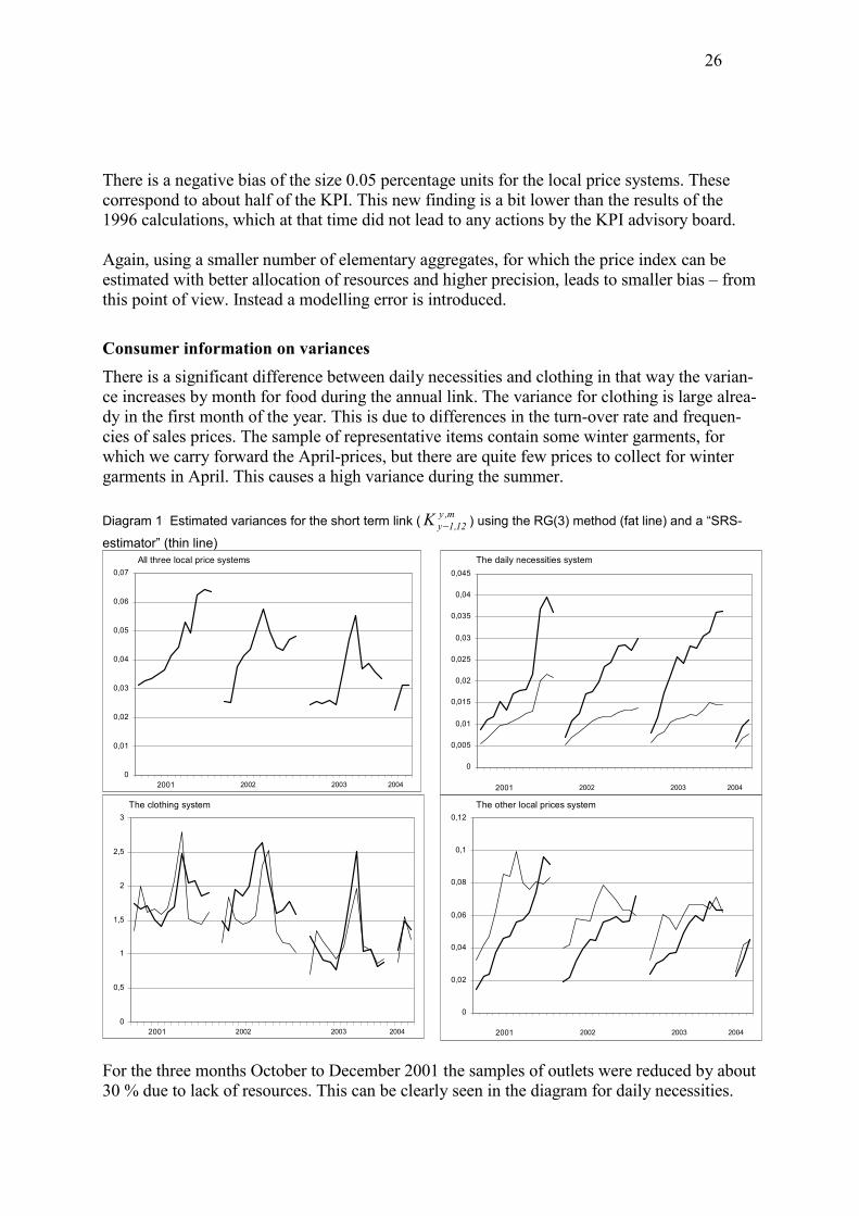
Consumer information on variances There is a significant difference between daily necessities and clothing in that way the varian-ce increases by month for food during the annual link. The variance for clothing is large alrea-dy in the first month of the year. This is due to differences in the turn-over rate and frequen-cies of sales prices. The sample of representative items contain some winter garments, for which we carry forward the April-prices, but there are quite few prices to collect for winter garments in April. This causes a high variance during the summer. Diagram 1 Estimated variances for the short term link ( m,y

12,1yK − ) using the RG(3) method (fat line) and a �SRS-

estimator� (thin line)

0

0,01

0,02

0,03

0,04

0,05

0,06

0,07

2001 2004

All three local price systems

2002 2003 0

0,005

0,01

0,015

0,02

0,025

0,03

0,035

0,04

0,045

2001 2004

The daily necessities system

2002 2003

0

0,5

1

1,5

2

2,5

3

2001 2004

The clothing system

2002 2003 0

0,02

0,04

0,06

0,08

0,1

0,12

2001 2004

The other local prices system

2002 2003

For the three months October to December 2001 the samples of outlets were reduced by about 30 % due to lack of resources. This can be clearly seen in the diagram for daily necessities.

27

For the daily necessities system the variance is larger than had the sample been drawn independent in each outlet. This is indicated by the �SRS-variance� being smaller. The probability samples of both outlets and product offers can only be put into practice if we have a small number of product samples. If we were to draw one product sample for each outlet, independently or negatively coordinated, we would have a heavy work-load to keep them updated. Diagram 2 Estimated variances for the inflation level, using the RG(3) method

0

0,02

0,04

0,06

0,08

0,1

0,12

2001 2004

All three local price systems

2002 2003

0

0,01

0,02

0,03

0,04

0,05

0,06

2001 2004

The daily necessities system

2002 2003

0

1

2

3

4

5

6

2001 2004

The clothing system

2002 2003

0

0,02

0,04

0,06

0,08

0,1

0,12

0,14

2001 2004

The other local prices system

2002 2003 Clothes are again a problem, there is a seasonal pattern with high variances in June-August. There are, probably, some product groups among all other goods in the other local prices, for example footwear, where we have the same problem. The variance of the inflation level is smallest in December. This is explained by the fact that this is the only month when the inflation level is equal to a short term index link and for this we have only one sample of outlets and representative items and no update of weights. For other months than December a rough rule of thumb could be to multiply the variance of the December link with 1.5 to get the variance of the inflation level.

28

Diagram 3 Estimated variances for the monthly change of inflation, using the RG(3) method

0

0,01

0,02

0,03

0,04

0,05

0,06

0,07

0,08

2001 2004

All three local price systems

2002 2003

0

0,005

0,01

0,015

0,02

0,025

0,03

0,035

1 4 7 10 13 16 19 22 25 28 31 34 37 40

2001 2004

The daily necessities system

2002 2003

0

1

2

3

4

5

6

2001 2004

The clothing system

2002 2003

0

0,01

0,02

0,03

0,04

0,05

0,06

0,07

0,08

2001 2004

The other local prices system

2002 2003

The seasonal pattern for clothing is very clear and it has a significant impact on the total of the retail trade good and services. The change of the inflation level is approximately the difference between a monthly price change from month y,m-1 to y,m and from y-1,m-1 to y-1,m. If the change of inflation is the most important statistic, more resources should be spent on the clothing survey, as pointed out above.

6 Conclusions and discussion

The use of two-dimensional designs with elements of non-probability sampling methods, annually updated samples and complex estimators creates problems when estimating sampling variances for CPI-statistics. Dalén and Ohlsson (1995) worked out a variance expression for the Swedish CPI index link in the daily necessities system by Taylor linearisation. They also proposed an estimator for the variance. The daily necessities system has one probability sample of outlets and three samples of products, one for each of the three outlet chains that have a dominant market share in trade in daily necessities in Sweden. A resampling method for variance estimation could be attractive to estimate more complex statistics, such as the twelve-month-change (inflation level) and the monthly change of the twelve-month-change of index. Such methods do not bring more information on the

29

underlying structure of variation, which we need for efficient allocation of resources. For this purpose we have used analysis of variance models. We have developed these models not only to see the structure, but to estimate the sampling variance. This estimator, however, is not practical for complex situations like this. We have carried out a simulation study to compare three estimators of a random groups type with the Dalén and Ohlsson�s estimator and the model-based estimator. Price data for We have learned that the following procedure creates reliable results: Sub-sample a proportion

)2/(1 )1(π− of the outlets and a proportion of ( ))2()1( 111

ππ −⋅+ of representative items

independently in each outlet, where )1(π are sampling probabilities for outlets and )2(π are sampling probabilities for products. The latter don�t exist for most product groups because of judgemental selection of representative items and must be set rather arbitrary. A large number of such sub-samples, say 1 000, are selected. It is important that these sub-samples are coordinated for all years in study so as to reflect the annual update of samples and sampling probabilities. For each sub-sample the function of index links is computed and a mean of squared deviations is the variance estimator. We have learned that more of the resources should be spent on the clothing survey because the variance is very large. For product groups where the price collector makes a selection of a product offer to price, the variation in price data can be regarded as a variation between product offers to a large extent and only little variation can be explained by outlet or product group. As the cost of price collector�s traveling is substantial, this implies that the samples of outlets should be quite small. We have seen a significant seasonal pattern in the indices for clothing, especially in the monthly change of the twelve-month-change. This is due to the lack of special summer-garments in the sample and the carrying-forward of a small number April prices for winter-garments. Prices for clothing also changes very quickly which makes clothing a bigger problem for precision in the monthly change of the twelve-month-change then in the level of the twelve-month-change. For sample allocation, it is necessary to decide which of these statistics is most important.

30

7 References

Dalén, J. (1992) �Computing Elementary Aggregates in the Swedish Consumer Price Index�, Journal of Official Statistics, Vol. 8, No.2, 129-147. Dalén, J. (1999) �Bedömning av biasrisker i konsumentprisindex (KPI)�, Annex 6 to SOU 1999:124. Dalén, J. and Ohlsson, E. (1995) �Variance Estimation in the Swedish Consumer Price Index�, Journal of Business & Economic Statistics, July 1995. Vol 13, No.3 Jönrup, H. (1974) �Estimation of variances in multistage sampling�, Statistisk tidskrift 1974:5 Norberg, A. (1999): Quality Adjustment � the Case of Clothing. In Proceedings of the Measurement of Inflation Conference, edited by M. Silver and D. Fenwick. Cardiff University, pp. 410�426. Ohlsson, E. (1990) �Coordination of Samples Using Permanent Random Numbers�. In Cox et al: Business Survey Methods, Wiley, pp. 153�169. Ohlsson, E. (1995) �Sequential Poisson Sampling From a Business Register and its Application to the Swedish Consumer Price Index�, R&D Report 1990:6, Statistics Sweden Raj, D. (1968) �Sampling Theory�, McGraw-Hill Rosén, B. (2000) �A User´s guide to Pareto π ps Sampling�, R&D Report 2000:6, Statistics Sweden Statistics Sweden (2001) �The Swedish Consumer Price Index. A handbook of methods�, http://www.Statistics Sweden.se Wolter, K. (1985), �Introduction to Variance Estimation�, Springer-Verlag.