Embed Size (px)
Citation preview

Scholars' Mine Scholars' Mine
Masters Theses Student Theses and Dissertations
1968
Evaluation of methods for analysis of multi-degree-of-freedom Evaluation of methods for analysis of multi-degree-of-freedom
systems with damping systems with damping
Brijgopal R. Mohta
Follow this and additional works at: https://scholarsmine.mst.edu/masters_theses
Part of the Mechanical Engineering Commons
Department: Department:
Recommended Citation Recommended Citation Mohta, Brijgopal R., "Evaluation of methods for analysis of multi-degree-of-freedom systems with damping" (1968). Masters Theses. 5272. https://scholarsmine.mst.edu/masters_theses/5272
This thesis is brought to you by Scholars' Mine, a service of the Missouri S&T Library and Learning Resources. This work is protected by U. S. Copyright Law. Unauthorized use including reproduction for redistribution requires the permission of the copyright holder. For more information, please contact [email protected].

EVALUATION OF METHODS FOR ANALYSIS OF
MULTI-DEGREE-OF-FREEDOM SYSTEMS
HITH DAMPING
BY
BRIJ. R. HOHTA 1 \ C,qL
A
THESIS
submitted to the faculty of
THE UNIVERSITY OF MISSOURI AT ROLLA
in partial fulfillment of the requirements for the
Degree of
MASTER OF SCIENCE IN HECHANICAL ENGINEERING
Rolla, Missouri
1968
_ Approved by
~ (advisor)
. })yf 111.
ii
ABSTRACT
A general review of various methods for studying the behavior of
linear lumped parameter systems with viscous damping is presented.
Five methods are discussed. These are: (1) Normal Mode Technique
(2) Holzer's Method (3) Impedance Method (4) Graphical Technique (5) A
Method for Reducing Degrees-of-freedom.·
For solution of vibration problems by the Normal Mode Technique,
the systems are classified as (1) classically damped or (2) non-classically
damped. It is shown that the classically damped systems are relatively
easy to solve. For non-classically damped systems, the method proposed
by K. A. Foss has been employed. This method is quite complex, but does
provide an exact solution in most cases. In Holzer's Method, equations
for both undamped and damped systems are derived. A sample table is
presented which is employed to solve these equations. Systems having
dampers between masses as well as between the masses and ground have been
discussed. Also branched systems have been treated. In the Impedance
Method, the four-pole parameters of a mass, spring and damper are derived
and the formulas for solving tandem and parallel connections are pre
sented. In the Graphical Technique, procedures for arranging the equa
tions of motion in a form suitable for graphical solution are outlined.
Application of this method to branched systems is discussed. In the
Method for Reducing Degrees-of-Freedom, two problems are presented to
illustrate the use of this method. The results obtained have been com
pared with exact solutions.

iii
Advantages and disadvantages of each of these methods are discussed
on a comparative basis. A sample problem is solved by all of these methods
and the results are compared. Suggestions for further work are made.

ACKNOwLEDGEMENTS
The author is grateful to Dr. William S. Gatley for the
suggestion of the topic of this thesis and for his encouragement,
direction, and assistance throughout the course of this thesis.
Financial assistance in the forms of a graduate assistant
ship from the Mechanical Engineering Department and a research
assistantship from the Engineering Hechanics Department of the
University of Missouri at Rolla was certainly appreciated.
iv
The author is thankful to Mrs. Johnnye Allen for her wonderful
cooperation in typing this thesis.
TABLE OF CONTENTS
·page
LIST OF FIGURES • • vii
LIST OF SYMBOLS • . . . . . . . . . . . . . . . . ix
I. INTRODUCTION 1
II. REVIEW OF LITERATURE . . . . . . . . . . . . . 3
III. ANALYSIS OF D.AHPED MULTH1ASS SYSTEMS 5
IV. NOR11AL MODE TECHNIQUE • • • 6
Derivation of Equations of Hotion of Hulti-Degree of Freedom System • • • • • • • • • 7
Undamped Sys terns • • • • • • • • • • • • • 12 Damped Systems • • • • • • • • 15
V. HOLZER' S METHOD • • •
VI.
Undamped System • Selection of Trial Frequencies Forced Vibrations Branched Systems Damped Systems
IMPEDANCE METHOD
VII. GRAPHICAL TECHNIQUE •
Derivation of Equations • Branched Systems • • • • Graphical Method for Solution •
VIII. METHOD FOR REDUCING DEGREES-OF~FREEDOM
Illustrative Examples •
IX. SUM}f.A.RY AND CONCLUSIONS • •
X. SUGGESTIONS FOR FURTHER WORK
. .
BIBLIOGRAPHY . . . . . . . . . . . . . . . .
. .
. . .
. . .
. . .
. . .
.
.
.
.
23
24 27 29 30 35
40
47
47 54 57
62
64
75
82
83
v

APPENDICES
APPENDIX A APPENDIX B APPENDIX C APPENDIX D
. . . . . . . . . . . . . . . . . Reciprocity Theorem • • • • • • • • Review of Hatrix Operations • • • • • Parallel Four-pole Networks • • • • • • Sample Problem • • • • •
. 85
• 86 89
• 95 . 96
98 Normal Mode Technique • • • • • • Holzer's Hethod . • • • • 105 Impedance Method Graphical Technique Reduced System
. . . . • • • • • • 111 • • • • • • • • 117 • • • • • • 122
Comparison of Results by Various Methods • 127
VITA • • • • • • . . . • • . • . • · • • • · • • · • • • . 129
----------------------~ --------
vi

vii
LIST.OF FIGURES -------Figure
1. Hass, Spring, and Damper System •• 8
2. A Three-Disk Torsional System . . . . . 25
3. A Geared Torsional System • • . . . 31
4. Equivalent System With One-to-One Gearing • 34
5. A Damped Torsional Multidisk System • 36
6. Four-pole Parameter Notation 40
7. Two Four-pole Elements Connected in Parallel 45
8. Damped Hulti-degree-of-freedom System • • • • • 48
9. Damped Four-degree-of-freedom System Excited by
Foundation Motion • • • • • • 55
10. Td l1agnitude and Phase-angle Characteristics 58
11. Tf Hagnitude and Phase-angle Characteristics . . . 59
12. A Spring--Mass System . . . . 65
13. Reduced Spring-Hass System . . . . . . . . . . . 68
14. A Spring-Mass System . . . . . . . . . . . 70
15. Reduced Spring-Hass System . . . . . 73
16. Equivalent Reduced System • . . . . . . . . . 73
17. A Simply Supported Beam With 1'--;.;o Loads . . . . . . . . 87
18. A Damped Three Degree-of-freedom System Excited by
Foundation Motion • • • • • 97
19. Remainder Displacement From Holzer's Method • . . . 107
20. A Damped Three Degree-of-freedom System With Harmonic
Excitation . . . . . . . . . . . . . . . . . . . . . . 113

Figure Page
21. A Damped Three Degree-of-freedom System 'Vith Harmonic
22.
23.
24.
Excitation . . . . . . . . . . . . . . Vector Diagram for the Graphical Technique
Initial Reduction of the Original System
Reduced Two Degrees-of-freedom System • • • •
. . .
118
121
123
123
viii

=
=
=
LIST OF SY11BOLS
(Listed in order of appearance) displacement coordinate associated with ith mass,
velocity of ith coordinate,
acceleration of ith coordinate,
Cij = coefficient of viscous damping between ith and jth mass
Kij -- spring constant bet\veen i th and j th mass
=
=
=
=
=
u =
v =
p =
w =
Mi =
[Q] =
[N) =
[r] =
= a ne Ji :::;
ai =
ei =
ai =
force on the ith mass
displacement of ith normal coordinate
velocity of ith normal coordinate
th acceleration of i normal coordinate
kinetic energy
potential energy
dissipation function
virtual work
circular frequency
mass of ith element
modal matrix
identity matrix
a constant
mass moment of inertia of ith disk
angular displacement of ith disk
angular velocity of ith disk
angular acceleration of ith.disk
{!iJ = a column vector of amplitudes in 2N space
ix

= four pole parameters
w = selected value 0
of w within frequency range of interest
Tdj = displacement transmissibility of jth element
Tfj = force transmissibility of jth element
w0
j = individual natural frequency of th
j spring-mass system
= ratio of viscous damping to the mass-damper system.
C · ;;i 2 - 4KiMi, =- _::.J.. +
2Mi - 2Mi
critical damping of jth spring-
= th coefficient of viscous damping between i .mass and ground
A~B~C~ = as defined in context
S = phase angle
X

1
I. INTRODUCTION
It should be remarked at the outset that this is a report of the
tutorial type. By this, it is meant that many of the methods to be
presented have appeared somewhere in the literature. However, engineers
with only basic knowledge of the subject of vibrations often have diffi
culty in understanding and applying these ideas, many of which are pre
sented in relatively obscure forms. The purpose here is to collect
these ideas together and to describe, evaluate, and compare them in such
a way that the method best suited to solution of a particular problem
can be determined and applied.
Many engineering vibration problems can be treated by the theory
of one-degree-of-freedom systems. More complex systems may possess
several degrees of freedom. The standard technique to solve such systems,
if the degrees of freedom are not more than three, is to obtain the
equations of motion by Newton's law of motion, by the method of influence
coefficients, or by Lagfange's equations. Then the differential equa
tions of motion are solved by assuming an appropriate solution. Solving
of differential equations of motion becomes increasingly more laborious
as the number of degrees of freedom increases. While the solution is
straight forward for an undamped multi-degree-of-freedom system, it
becomes much more complex for a damped system.
The forces Fi arising due to damping associated with the co-ordinates
xl, x2, - - - - -, ~ will have the form

F damp n
= -
. c nn x n
For a less accurate solution, the damping forces associated with the
normal coordinates can be written as:
Fl
F2
F damp n
cl 0
0
=
0
0 0
c2 0
0 c3
0
0
0
c n
. nl
n2
2
Note that the off-diagonal, or coupling terms have been assumed negligibly
small. However, for many engineering applications such as aircraft design,
this method fails to provide an accurate solution. For this reason
several different techniques have been suggested for solving a damped
multi-mass system.
The objective of this thesis is to analyze, simplify, and compare
these techniques in a manner useful to practicing engineers. To facilitate
this, a sample problem will be solved by each of these methods. This
will also be of value in illustrating the use of the mathematical theory
presented.

3
II. REVIEW OF LITERATURE
(1 2 3 4)* Generally textbooks ' ' ' very thoroughly cover the analysis
of undamped multimass systems, with practically no mention of damping
in such systems. The only exception to the above statement is reference
(2) where the author has derived the equations of motion for a damped
n-degree-of-freedom system and has also presented an approximate solution
for such a system.
Because of the wide applications of damped multimass systems,
several technical papers with different solutions to the problem, have
(11) (12) appeared recently. K. A. Foss , T. K. Caughey , and M. E. J.
O'Kelly(l3) have developed the Normal Mode Technique which is widely
used in solving the equations for damped multimass systems. However,
this method has limitations which will pointed our later.
In a modification of the Normal Mode Technique, S. E. Staffeld(7)
has suggested a method by which the number of degrees of freedom can
be reduced in mathematical models of damped linear dynamic systems.
(1) (8) (9 10) . W. T. Thomson , E. H. Eddy , and J. P. Den Hartog ' descr1be
and demonstrate the use of Holzer's method, which is one of the most
j_mportant tools in solving damped torsional multidisk systems.
C. T. Molloy!S) has suggested the use of four-pole parameters for
solving vibration problems. The graphical technique of reference (6)
* Numbers in parentheses refer to the list of references at the end of the thesis.

is also quite useful in determining the frequency response of linear
mechanical systems.
4

5
III. ANALYSIS OF DAMPED MULTI}~SS SYSTEMS
Several methods are available for analyzing a damped multi-degree
of-freedom system. Some of these will be presented here in the following
order:
1. Normal Mode Technique
2. Holzer's Method
3. Impedance Method
4. A Graphical Technique
5. Method for Reducing Degrees-of-freedom
Where the development of mathematical theory is complicated,
undamped systems will be considered first and then damping will be intro
duced in such systems. In other methods which are easier to follow,
undamped systems are considered as a special case of the general problem
with damping. Should it be desired to apply these methods to an undamped
system, the damping term is simply set equal to zero.

6
IV. NORMAL MODE TECHNIQUE
The equations of motion of a system can be derived by a number of
different methods. These are derived here by using Lagrange's Equa
tions(l4), the energy method most frequently encountered in engineering
analysis.
To use Lagrange's equation, it is necessary to define:
(1) Generalized Coordinates: A set of independent coordinates used
to completely describe the motion of a system.
(2) Holonomic System: A system such that the number of degrees of
freedom equals the number of coordinates required to completely de-
scribe it.
(3) Non-Holonomic System: For such a system, the number of degrees
of freedom is less than the required number of coordinates required
to completely describe the motion of the system. In such systems
coordinates cannot be eliminated by using the constraint equations.
TI1erefore, systems containing non-holonomic constraints always require
more coordinates for their description than there are degrees of freedom.
Such systems may occur in Dynamics of Particles(l4) but are rarely
encountered in vibration analysis.
Lagrange's equations for a holonomic system with n degrees of
freedom can be expressed as
(1)

7
Here V is a dissipation function which accounts for the losses
due to viscous damping. P is virtual work. The concept of virtual work
is explained(l4) as follows:
Suppose that the forces F1
, F2
, .•.•• , FN are applied at the cor
responding coordinates in the direction of the increasing coordinate
in each case. Nmv imagine that, at a given instant, the system is given
arbitrary small displacements ox1 , ox2 , •.•• , oxN of the corresponding
coordinates. The ,.;rork done by the applied forces is
and is known as the virtual work. TI1e small displacements are called
virtual displacements because they are imaginary in the sense that they
are assumed to occur without the passage of time, the applied forces
remaining constant.
DerivatJon o~ Equations of Motion of Multi-Degree of Freedom System
Consider a system of n discrete masses m. coupled together through l.
springs and dashpots as shown in figure 1. Let xi denote the n general-
ized coordinates to specify the motion of the system.
for all i when the system is in stable equilibrium.
n 1 ~ . 2
T = 2 I.. mixi i=l
Define xi = 0
For such a system,
(2)
(3)

( (.-1 L ,
Figure 1
.....__,---J M l.+ 1 K~-t 1, L +a a----;,_ )( ~ + 1
Ci+t
Mass, Spring, and Damper System
8
Mttz.
xi..+2

n
I 1 V=2 i=l
From these equations,
oP oxi =
It can be shown by use of the reciprocity theorem* that
Using the above relationships,
* for proof, see Appendix A.
** The notation is explained as follows:
Let i = j = 2
Since K12 = K21
1 2 1 2 U = 2 Kllxl + Kl2xlx2 + 2 K22x2
au ·-=
au --= Kllxl + K22x2 + Kl2xl + K12x2
2
I Kijxj j=l
for i = 1,2 =
Similarly for i = 1,2, •• • n.
9
(4)

av ax
1 =
n
) c1 jxj J=l
Substituting the above expressions in equation (1), the equations of
motion for the system may be written
i = 1,2, •.
The above equation can be represented in matrix form as
where
Mass Matrix
Spring Mat·dx
*
[M) {}{} + (C) {x} + [K] {x} =· {F}
0
0 0
0
0
M n
K nn
• , n
(5)
(6)
10
Here Fi is sinusoidal in nature. For discussion of solution with other forms of forcing function, refer to section (IX).

Damping Matrix
[c] =
{x} =
and {F} =
cnl
xll x2 . . X n
Fl F2
F n
.. c nn
a column vector of order Nxl
a column vector of order Nxl
For a physically realizable system~ [MJ,[KJ~ and [c) are symmetric
matrices. This follows from the fact that the system obeys the reci-
procity theorem. Also [M] is a diagonal matrix if the motion of each
mass is described by a different absolute coordinate.
A review of the properties of matrices useful for vibrational
analysis is given in Appendix (B).
11

12
Undamped Systems:
For undamped systems, equation (6) reduces to
[M]{x} + (K){x} =· {F} (7)
To solve this set of equations by classical methods it is necessary to
first solve the homogeneous equation
[M]{x} + [K]{x} = o (8)
This equation is also known as the equation of free vibrations of the
undamped system.
The equation (8) can be solved by assuming a solution of the form
{x} = {q} iwt e (9)
where {q} is a column vector of order Nxl, the elements of which are
independent of time. On substituting equation (9) into equation (8),
or
(10)
For non-trivial solutions(l7) of equation (10),
(11)
Equation (11), known as the characteristic equation, is a polynomial
of degree n in w2 when the above determinant of order n is expanded.
Since both [M] and (K) are symmetric and positive definite, the roots
of this equation are all real and positive(lS). Neglecting for the
present the case of repeated roots, there exist n distinct values of
2 2 w which satisfy equation (11). For each distinct wi there exists a

13
i vector {q } which satisfies the following equation:
[-wi z(MJ + [KTI {qil = o
TI1e vectors {qi} form a linearly independent set(lJ).
Since [M] and [K] are symmetric and positive definite, there exists
a transformation(lB)(Q]such that
[Q] T [M] [Q] = [M] a diagonal matrix
[Q] T [Kj [~ = [k] a diagonal matrix
where Q is known as the 11odal Hatrix, the columns of which are the
eigenvectors of the system.
The particular solution is obtained by letting
{x} = [Q]{n(t)}.
On substituting equation (12) into equation (7)
[M)[Q)Oi(t)} + [K)fQ){n(t)} = {F{t)}
T Premu1tip1ying equation (13) by fQ] ,
or
where
and
[M]{n(t)l + lK]{n(t)} = {G(t)}
(Q}T{F(t)} = {G(t)}
{G(t)} = g1 (t)
g2(t)
g (t) n
(12)
(13)
(14)

Equation (14) is a system of uncoupled equations of type
(15)
where --= The complete solution of equations (15) is
pi ni = Acoswit + Bsinwit + K _ M w2 coswt
ii ii
where A and B are constants of integration to be determined by the
initial conditions and gi is
xi is obtained from equation
xl
x2
X n
= ~1
of the
(12).
2 q
1 2 where the column vectors q , q , •
system.
form P icoswt. Having found ni'
Thus
nl
.q_j n2
•
n • , q are the eigenvectors of the
From the above analysis it is evident that any undamped forced
system can be solved by the Normal Mode Technique provided the roots
14
of the frequency equation are distinct. This method has been presented
in great detail in reference (2) and the author has solved several
representative problems.
For the case of repeated roots, see Appendix (B) where the pos-
sibility of a solution with repeated roots is discussed.

Damped Systems:
For the purpose of analyzing damped systems, we shall divide
such systems into two categories:
(a) Classically Damped Systems are those systems in which the matrix
15
(C J is also diagonalized by the same transformation which uncouples the
corresponding undamped system.
{b) Non-classically Damped Systems are those where [CJ cannot be dia
gonalized by the transformation which uncouples the corresponding un
damped system.
Classically Damped Systems:
For a linear damped system, the equations of motion are
[M]{x} + (C){x} + [K){x} = {F(t)} (16)
where [C] is symmetric and non-negative definite.
As sho'tvn in Appendix B, there exists a transformation (Q] such that
[Q)T tM)[Q) = tH)
[QJ T (K)t_Q) = (K)
Now if @]is such that
is a diagonal matrix
is a diagonal matrix
is a diagonal matrix
then it is possible to completely uncouple the above equations of
motion.
Let {x} = [Q]{ n (t)} (17)

Substituting equation (17) into equation (16)
[M][Q){n(t)} + [c)(Q1{n(t)} + (K][Q){n(t)} = {F(t)}
Premultiplying the above equation by [Q)T,
(Ql(M][Q]{n(t)} +[Q] T(C)[Q.){n(t)} + [Q)T[K][Q]{n(t)} =
[M]{n(t)} + fc]Ul(t)} + t'KJ{n(t)} =· {gi(t)}
This is a set of uncoupled equations of type
Mi.n. +c .. rii + K .. n. = gi(t) ~ ~ ~~ ~~ ~
TI1e complete solution is of the form
where gi = Pi coswt
16
T (Q) {F(t)}
c1 and c 2 are constants of integration to be determined by initial
conditions.
Thus, in a classically damped system, it is always possible to obtain
a solution of type
{X}= [Q]{n}
where [Q] simultaneously diagonalizes (MJ .1[K),and [c] •
The above analysis is possible only if [ C J is such that the trans-
formation which uncouples the undamped system will also uncouple the
damped system. Dr. T. K. Caughey(l2) derived sufficient conditions for
( C J such that the equations can be uncoupled as above. However, the
necessary conditions for uncoupling the damping matrix have not yet been
developed.

17
Caughey shows that a sufficient though not necessary condition that
The above expression is arrived at by making use of the transformation
{X} = [N]{L} and reducing the equations of motion to the following form
where
and
[I]{L} + (A]{L} + (B){L} = 0
(A] = (N)-1[c)(N)
(B)= (Nll (K)(N)
It is then proved that if diagonal matrices (a] and [b1, obtained from
(A) and (B] respectively by some other transformation, can be expressed
as (a] = (b]t where t is t an integer then [A]= (B] • Thus, if [A1 = [B]t,
it can be concluded that (a) = [b]t. By a more extensive analysis on
similar lines, Caughey's sufficient condition can be derived. Caughey's
condition is equivalent to stating that if (C) can be expressed as a
linear combination of [M] and [K],then the system is classically damped.
Non-classical~ Damped Systems:
If the system possesses non-classical damping, the methods of
solution presented above are not applicable. K. A. Foss(ll) has developed
a method for solving some of these systems. In this method the original
system is transformed in 2N space in which the equations of motion of the
system can be uncoupled.

Method of K. A. Foss
We define a pair of 2Nxl column vectors
{Z} = r {x} l ~ {x} {
{
{0} l . {F} = {F(t) I
and the following set of matrices of order 2Nx2N
[P) = j-(M1 [0~ L [o) [Klj
18
where {xJ~ 1*1~ {OJ and F(t) are column vectors of order Nxl associated
with the equations of motion. With the above definitions the equations
of motion of the original system can now be reduced to
[R]{Z} + (P] {Z} = {F(t)} (18)
The above equation, after performing the indicated matrix operations,
results in two matrix equations~ one of which is the original equation
of motion and other is an identity. Thus
or
and
fTo1 [M)l {on} + [-(M] (o~ f {x} { f {O} l lfMJ [cJJ {x} [o) (Kn 1 {x}! = 1 {f(t)} J
[M]{*f - lM] jxJ = {o}
[M]{x} + (c) {x} + (K){x} = { f (t)}

19
To obtain a solution of equation (18) we first solve the homogeneous
equation lR){Z} + (PJ{Zf ={Of
Assume fz}= {{~~} = e o<t{~f= eo(t[1~J on substituting equation (20) in equation (19) and rearranging
(19)
(20)
[c<:[R) + (PJ] {f-J = {of (21) -1
Premultiplying by L P] and dividing through by <>e , the a hove equation
becomes
It is easily shown that
(P J -1
[
-1 - [M]
[O] (OJ J [Kr1
and therefore it will always exist. Thus, I
== [o] 1 - [r) -- -:t--LK] -l [ M]l [K)-1lc]
Equation (22) now becomes I
(22)
== [u]
(23)
Equation (23) is the usual form of an eigenvalue problem. tu] will be
symmetric only if - tl] and
lK]-l [c) is a symmetric matrix
If (u) is symmetric, then 2N independent eigenvectors will always exist
(as shown in Appendix B) and Foss's method will give a solution. However,
in general (u] is unsymmetric and 2N linearly independent eigenvectors
will always exist only if there are 2N distinct roots of the frequency
equation in 2N space
ll[[u] + ~ [rJ]ll == 0 (24)
For each distinct root 1 --- of the above equation there exists an independent vCi

20
. i vector {~ }. As shown in Appendix B, a root of multiplicity K may or
may not have K associated linearly independent eigenvectors. TI1e eigen-
values of the system are obtained by solving equation (24). Equation (23)
then gives the eigenvectors ~i} in 2N space. i . .
Having found {! }, {xi}
can be obtained from equation (20).
Forced Vibrations
Nonhomogeneous solution of the equations of motion in 2N space is
obtained by letting
{z J = [o]{~}
where [Q] is a matrix of order 2Nx2N, the columns of which are { p j andt~jis a column vector of order 2Nxl.
Using the orthogonality condition in 2N space, equation (18) reduces to
(25)
where Ri is a scalar and is defined as
The solution of equation (25) is
where Ai is an arbitrary constant depending upon initial conditions.
Having found ~i' {Z} is obtained from {Z} = ~¥~}.
S{x} J Since {z}::[ {x} , {x} can be obtained by expanding. {Z}.

21
The detailed derivations for forced vibrations are given in references
(11) and (13).
Limitations of Foss's Method: For the application of Foss's method,
it is assumed that
{Z} = f*l }= e<><tq_} = e-<t{~~ f {x} (26)
Since {x} = ec.<t{~}
{x} o(,t .
and = e {a<~}, (27)
{Z} =Q(e.ctr(: 1 (28)
It is shown below that for critically damped systems, equation (27) does
not apply.
Consider a critically damped system such that the ith uncoupled
equation
has the solution of type
\vhere , and
Ai and Bi are constants.
Here
and

22
therefore in this case.
(29)
The time derivative of the above equation cannot be expressed in the form
of equation (28) and therefore Foss's method does not give a solution
for critically damped systems. Summarizing, Foss's metho~ does not work
for the case
(1) where eigenvalues are repeated and the eigenvectors do not form a
linearly independent set.
(2) when the system is critically damped at one or more of its modes of
free vibration.
23
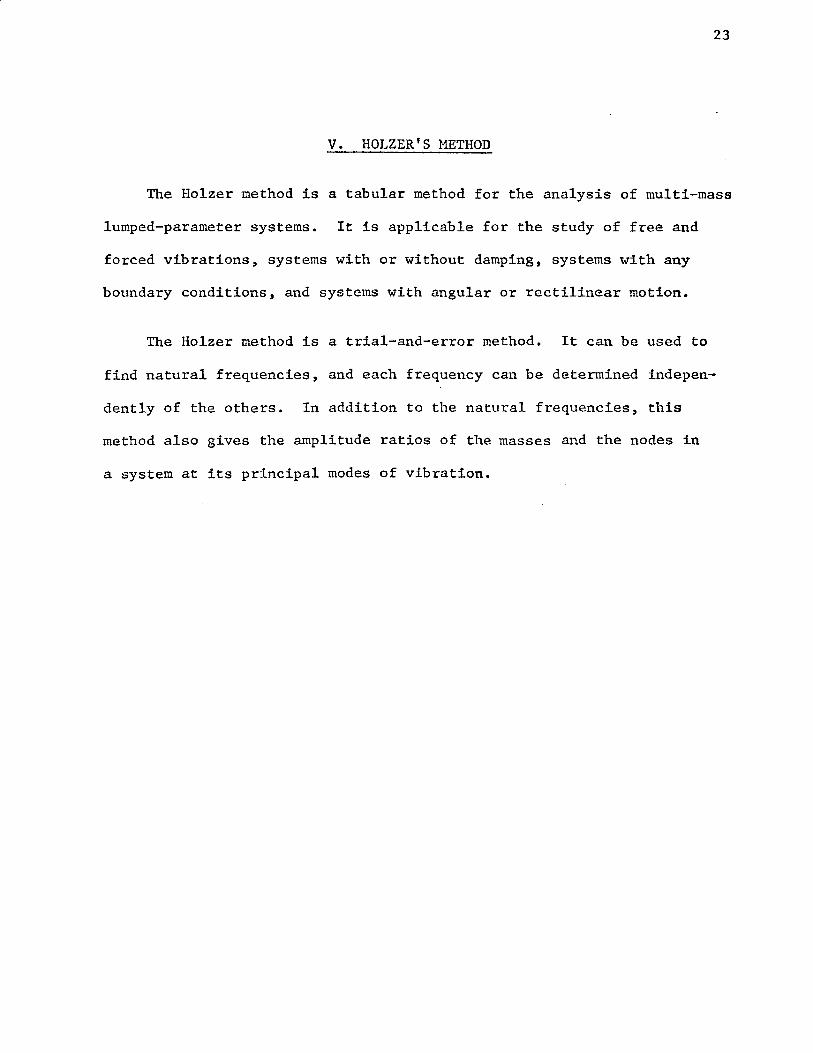
V. HOLZER'S METHOD
The Holzer method is a tabular method for the analysis of multi-mass
lumped-parameter systems. It is applicable for the study of free and
forced vibrations, systems with or without damping, systems with any
boundary conditions, and systems with angular or rectilinear motion.
The Holzer method is a trial-and-error method. It can be used to
find natural frequencies, and each frequency can be determined indepen
dently of the others. In addition to the natural frequencies, this
method also gives the amplitude ratios of the masses and the nodes in
a system at its principal modes of vibration.

24
Undamped System:
For an undamped system, it can be assumed that no external torque
is required to maintain a conservative system vibrating at its principal
modes. Consider the system shown in figure 2. The equations of motion
are
318
1 + K12 <a 1 - a 2> = 0 (30)
.. - K12 <e 1 - a 2 > + K23 <8 2 - 8 ) 0 J2a2 = 3
(31)
338 3 - K2 3 <a 2 - a 3 > = 0 (32)
Summing the three equations gives
(33)
Hence the sum of the inertia torques must equal zero at all times.
The motions of all disks are simple harmonic. Letting
el = A coswt
82 = B coswt
83 = c coswt
and substituting for 81 and e2 in equation (30) above,
or
If A is taken as unity, B can be calculated.

25
-J", -
s~
Figure 2
A Three-Disk Torsional System

26
Adding equations (30) and (31),
or
C = B -
2 2 J 2Bw + J1Aw
K23
Knmving B, C can be calculated. Generalizing the above procedure,
i=-n-1 2 L Jie iw e = a - ic.....=.:::.l ____ _
n n-1 Kn n~l , (34)
Equations (33) and (34) provide the basis for the Holzer table which
is presented below:
Trial Frequency w ~-------------------------------------------------------------------------~
Station Hass Moment Jw2
Number of Inertia J
(1) (2)
Amplitude a
(3)
Inertia Torque J,.,43
(4)
Holzer Table
(5)
Spring constant K ·· .. i,~-1
(6) (7)
A similar table can be constructed for rectilinear motion if J is re-
placed by M and e by X.
The physical meaning of the various columns in this table is as
follows:
Column 2: is the inertia torque of each disk for an amplitude of 1 radian
at the trial frequency selected;
Column 3: is the angular ar.1plitude e of each disk;

Column 4: is the inertia torque of each disk at the amplitude a;
Column 5: gives the value of the shaft torque beyond the disk in
question;
Column 6: shows the torsional spring constants;
Column 7: gives the relative angle of twist between the disk in
question and the next disk.
27
The computations of the natural frequencies of an undamped system
by Holzer's Method are straight forward. Assuming a trial value for a
natural frequency, the process is carried out by letting the angular
displacement of the first disk arbitrarily be one radian. The angular
displacement of each disk of the system is found by repeatedly applying
equation (34) in a sequential fashion. If the algebraic sum of the
inertia torques is zero, that is, if equation (33) is satisfied, then
the assumed frequency is a natural frequency. If equation (33) is not
satisfied, a new value of w is assumed and the process is repeated.
The magnitude and sign of remainder torque are a measure of how far the
trial frequency is removed from a natural frequency.
Selection of Trial Frequencies:
The difficulties often encountered with the Holzer's Method are
(1) in estimating the initial trial value for w; and (2) in selecting
a second trial value for w if the initial trial value does not satisfy
equation (33).

28
The initial value of the trial frequency is usually obtained by
reducing the multidisk system to an approximate two or three disk system.
The approximate frequency to be assumed may then be found by using fre-
quency equations presented in Normal Mode Technique. A positive remainder
torque for the first natural frequency indicates that the system has
surplus inertia torque. Therefore to balance the system, a higher trial
value is selected. The reverse is true for a negative remainder torque.
Consequently the trial value is decreased. For torsional vibrations,
the mode of the vibration is usually taken to be the same as the number
* of nodes , which means that the first natural frequency has one node,
the second two, and so on. Each time a node is passed, the sign in the
amplitude column changes. The number of sign changes in the amplitude
column indicates the number of natural frequencies which lie below the
trial value. If there are many sign changes in the amplitude column for
the first trial, a much lower value of w should be selected for the next
trial.
To obtain the higher natural frequencies, it should be noted that
the inertia torque on the last disk changes sign as the frequency is
changed from below to above a natural frequency. A plot of remainder
torque as a function of trial frequency should be made to aid in the
estimation of trial frequencies (see sample problem). The points where
the curve intersects the frequency-axis should be used as trial eigenvalues.
* A node is a point along the shaft with a zero deflection.

29
To meet all possible boundary conditions, an appropriate Holzer
table has to be constructed. For example, if the left-hand end is
built-in, then e1
is required to be zero and an arbitrary value for
inertia torque on the first disk is selected. If the left-hand is free
then inertia torque is taken zero and e1 has some arbitrary value.
Similarly if right-hand is a free end, the torque at this end is zero
and if it is built-in, then the amplitude has to be zero.
Once the eigenvalues have been found, the amplitude column of the
Holzer table directly gives the eigenvectors for each of these eigen
values.
Forced Vibrations:
If a torque T0 coswt is applied to one of the disks, forced vibrations
will be produced. Consider the system of figure 2 except that in this
case a pulsating torque T0 coswt is acting on the first disk. It is re
quired to obtain the angular displacements of all disks which result due
to applied torque of frequency w. The equations of motion are
As before, let
J 18
1 + K
12 (e
1 - e 2) = T0 coswt (35)
J2e2 Kl2(el-e2) +K23(e2 -e3) = o (36)
J3e3 - K23(e 2 - e 3) = O (37)
e 1
= A coswt
e2 = B coswt
e 3 = C coswt
(38)

Substituting for e1 , e2 , and a3 in above equations of motion and adding
the resulting equations,
From equations (35) and (38),
B = A -
- T 0 (39)
The Holzer table is completed as before and the remainder torque is
equated to- T0 as indicafed by equation (39). This gives A in terms
of T0 • Knmving A, B and C can be calculated.
In the above example, the shaft considered is free-free and the
remainder torque is equated to - T • However, this may not always be 0
true. For example, if the last mass is attached to a rigid support,
30
then the remainder amplitude is equated to zero. Similarly other boundary
conditions have to be taken care of while solving forced vibrations
problems by this method.
Branched S~stems:
For use of this method in studying branched system behavior, separate
tables have to be made for each branch of the system. The application
of Holzer's Method to the branched systems can be best illustrated by
the following example: Consider the branched system shown in figure 3.
A Holzer table for branch 1 is made. Branch 1 is arbitrarily taken as
the primary branch with a unit angular deflection at the left-hand end.
Proceed through branch 1 as previously outlined to obtain the deflection

!!. K12.
1.-
Am pl. 1 llad.
c Js
JT
Ks-t> J6
~ 8-- ~67 1178
J_z. .J4 /'( 2. 3
J3 K34
Branch 2
~ L.. r,,
J9 K9.IO
J,o Branch 1 J{ JO,II
. -===o-· Branch 3
c
Figure 3
A Geared Torsional System
31
Ampl. lB

32
at section C-C. The calculation for branch 2 is started from the
opposite end at point 0. Assuming an arbitrary deflection of magnitude
B at this end where B is a constant, proceed towards section C-C. Since
the deflection at section C-C is already known, the two deflections are
equated to solve for B. The inertia torques of branch 1 and branch 2
are added. Calculations are then carried for branch 3 starting from
section C-C with inertia torque equal to the sum of inertia torques of
branch 1 and branch 2. If the trial frequency is a natural frequency
of the entire system, it will meet the boundary conditions at the end
of branch 3. If not, then the whole procedure is repeated for a new
trial frequency.
Use of this method requires that all branches of the system must
have a one-to-one gear ratio. This is accomplished by multiplying the
2* stiffness and mass moment of inertia of each geared shaft by n , where
n is the speed ratio of the geared shaft to the reference shaft. This
* If the oscillatory amplitude of reference shaft is a 1
, the oscillatory
amplitude of geared shaft will be a 2 = na 1 • The oscillatory kinetic
energy of disk 2 is then
1 . 2 1 2 . 2 T = 2 J 28 2 = 2 n J 26 1
2 and the equivalent inertia of disk 2 referred to shaft 1 is n J
2•
To determine the equivalent stiffness of geared shaft, note that
if e1
is the angle of twist of reference shaft, then the geared shaft
turns through an angle of na1 • The potential energy of the geared shaft

is illustrated in figure 4 which is equivalent of figure 3 with gears
reduced to common speeds.
(continued)
corresponding to twist of n 1
is
The geared shaft referred to shaft 1 must therefore have a stiffness
2 of n K2
•
TI~e energy dissipated due to viscous damping in the geared shaft
is
1 . 2 v = 2 c2e 2
Since 82 :::: nel
1 2 • 2 v = 2 (c2
n )e 1
The damping coefficient in the geared shaft referred to shaft 1 is
2 therefore multiplied by n •
Though the damping has not yet been introduced in the system, for
convenience, it has been discussed here.
33

J,
nl
n2
2 ,, /{67
Branch 2
Branch 1 2.. n2.J!>·
Branch 3
= S:2eed of branch 2 Speed of branch 1
S:2eed of branch 3 Speed of branch 1
Figure 4
Equivalent System With One-to-One Gearing
t n,J7
34
2. n, Ja

35
Damped Systems:
In an undamped system all disks move either in phase or out of
phase by 180 degrees with the disturbing torque and no energy is dis-
sipated. If damping is introduced into the system, the motion of each
disk will in general be out of phase by an angle other than 180 degrees.
Therefore the computational work is done in a mathematically complex plane
and computations are subject to the rules governing complex numbers.
The basic Holzer table equations for a general case may be derived
with the aid of figure 5. This includes viscous damping between the
disks as well as between the disks and ground. It is necessary to dis-
tinguish the viscous damping between the disks, which is designated as
Cij' from the viscous damping between the disks and the fixed member,
which is designated as hi·
Considering each disk as a free body, the following equations of
motion are obtained:
.. . + C12<91
. Jl91 + h191 + K12 (91 - 92) - 92) = 0 (40)
. J292 + h292 - K12(91 - 9 )
2 - c12 <91 - 9 ) 2
+ K23(92 - 93) + c23<92 - 93) = 0 (41)
. . - 93) J393 + h393 - K23(92 - 93) - C23<92 = 0 (42)
Since damping is present, complex numbers are used. Let
9i = Aiejwt
where j = v:T

36
h~
Figure 5
A Damped Torsional Nultidisk System
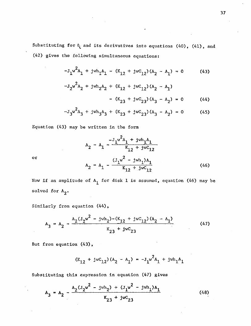
Substituting for et and its derivatives into equations (40), (41), and
(42) gives the following simultaneous equations:
- (K23 + jwC23)(A3 - A2) = 0 (44)
-J3w2A3 + jwh3A3 + (K23 + jwc23)(A3 - A2) = 0 (45)
Equation (43) may be written in the form
or
(46)
Now if an amplitude of A1 for disk 1 is assumed, equation (46) may be
solved for A2 •
Similarly from equation (44),
(47)
But from equation (43),
Substituting this expression in equation (47) gives
(48)
37

which may be solved for A3 by substituting in the calculated value of
A2 from equation (46).
Equation (48) may be written in general form for the motion of
disk i,
(49)
38
Equation (49) is a general form of the Holzer equation for damped systems
which may be solved in tabular form for an assumed value of A1
• Equa
tion (49) is similar to the corresponding equation (34) for undamped
systems. 2 Comparing the two equations, Jw term of equation (34) is
replaced by (Jw2
- jwh) in equation (49) and Ki i-l in this case be-, comes Accordingly, column 2 and column 6 of Holzer's
table presented previously have to be modified for damped systems.
Since vibrational energy is continuously dissipated in the form of
heat in a system having damping, any free vibration of such a system is
a transient one. The resonant frequency for a damped system has to be
defined in a different manner because the residual torque never passes
through zero(S). However, the remainder torque when plotted against
various trial frequencies has a minimum where the real part of the
torque passes through zero. This frequency can be designated as the
(22) damped natural frequency • \fuereas an undamped system vibrates with-
out any external torque at its natural frequencies, a damped system re-
quires an input to sustain such vibrations. Ho,vever, this input should
be minimum when the system passes through its natural frequencies.

This explains why the minimum point corresponds to one of the natural
frequencies of the damped system.
39
It should be mentioned that the above system had free-free boundary
conditions and therefore the remainder torque gave an indication of
natural frequencies. For other boundary conditions such as fixed-fixed,
the remainder amplitude has to be used in estimating a natural frequency.
The applications of Holzer's Method to damped systems with external
input and/or with branches is similar to that of undamped systems.

40
VI. !MFEDANCE METHOD
Use of the analogy between linear passive electrical networks and
a mechanical system can simplify the study of a complicated mechanical
system with either lumped or distributed parameters. The impedance
method(S) makes use of this fact and describes the steady state system
behavior.
Consider a mechanical system shown in figure 6. The elastic system
can be any combination of lumped, linear, mechanical elements such as
masses, springs, and dampers. It can also be combinations of linear,
distributed parameter systems, such as beams, plates. etc.
Fl Elastic F2 + Direction (1) v (2) System vl 2
Figure 6
Four-pole Parameter Notation
The elastic system must have two identifiable connection points
(1) and (2) which are called the input and output points respect-
ively. At the input point there exists an input force F1 and a
velocity v1
• The input force and velocity are produced by con
nection of point (1) to that portion of the complete mechanical
system which preceeds it. At the output point (2) there exists a
force F2
and a velocity v2
which result from the application of F1

and v1 at point (1) and the reaction of the portion of the passive
mechanical system between point (1) and point (2).
The performance of any component of the system can be described
by the following equations:
(50)
(51)
41
The four coefficients A11 , A12 , A21 , and A22 in the above equations are
called four-pole parameters. The four-pole parameters for a mass, spring,
and a viscous damper are obtained below.
Four-pole Parameter for ~Mass: Since the mass is regarded as a rigid
body,
(52)
and by Newton's law,
(53)
For a sinusoidal time variation motion, let
Fl FA iwt = e
F2 FB iwt = e
vl VA iwt = e
(54)
v2 VB iwt = e
where FA' FB, etc., may be complex functions of mass, stiffness, resis
tance, and frequency, but are time independent. Note that no phase
iwt angles are necessary in thee term since the FA' etc., terms are

42
allowed to be complex. The relations between velocity, displacement,
and acceleration can be expressed as follo,ITs:
v VA iwt = e
X !VA e iwt
dt VA iwt v = =- e =-iw iw
.. d (V) iwt X =- = iw VA e = iwv dt
Displacements at each input and output point are to be measured from
the respective equilibrium positions of these points. The equilibrium
position is defined as the position occupied by the point when no sinu-
soidal excitation is applied to the point.
Equations (52) and (53) become
(55)
(56)
Comparing equations (55) and (56) with equations (50) and (51), the
four-pole parameters for a mass are A11 = 1, A12 = imw, A21 = 0, and
Four-pole Parameter for ~Hassless Spring: The force applied at the
input point of the spring is the same as the force which the spring
delivers at its output point:
(57)
Also, (58)
The equations (57) and (58) can be written as

Vl = iw F + V K 2 2
Hence the four-pole parameters for a spring are A11
= 1, A12
= 0,
iw A21 = ~' and A22 = 1.
Four-pole Parameters for a Viscous Damper: For a damper,
and Fl = F2
F2 = C(Vl - v2)
(59)
(60)
where C is the coefficient of viscous damping. Rearranging equations
(59) and (60),
F1 = F2
+ o.v2
1 vl = c F2 + v2
43
and the four-pole parameters are A11
= 1, A12
= O, A21
= 1 C' and A22 = 1.
Connection of Four-pole Networks: There are two ways by which two
four-pole networks can be connected to each other;
(A) Tandem Connection
(B) Parallel Connection
(A) Tandem Connection: Two four-pole networks are said to be in
tandem connection when the output from the first is precisely the input
to the second. The analysis of this type of connection is efficiently
handled by matrix techniques. TI1e structure resulting from a tandem
connection of elements is simply another four-pole network. Equations
(50) and (51) can be written in the matrix form thus

(61)
where the subscripts signify that the parameters belong to the four-
pole network numbered (1).
If the output of four-pole network (1) is the input of four-pole
network (2), then
[::] = [A11: A12:] X [ ::J A21 A22
(62)
replacing [~Din equation (61) by its value from (62),
[::] = [All: A21~ [A112 A12~ X [ ::]
X 2 A222 A21 A22 A21
(63)
generalizing the above process for n networks in tandem,
A12l is obtained by multiplying parameter matrices of all A22j
the four-pole networks.
Note that each matrix in equation (63) is associated with a single
four-pole network and that any changes made in that network affect only
44
its own matrix. This is a considerable convenience in certain problems.
(B) Parallel Connection: When two four-pole networks are connected
so that

(1) all their input and output junctions move with the same velocity;
(2) the input force to the composite four-pole network is the sum of
the input forces of the individual networks;
(3) the output force from the composite four-pole network is the sum
of the output forces of the individual networks;
then the networks are said to be connected in parallel. A parallel
connection is shown below:
K
c Figure 7
Two Four-pole Elements Connected in Parallel
TI1e four-pole parameters for the composite system of n four-pole net
* work are given by the follmving formulas :
1 c = B' and A22 = B
where A R, i=n
A = r <A) i=l A21
i=n 1
B = r (~) i=l 21
i=n A R,
c = r <A) i=l A21
With the use of above equations, the four-pole parameters of the com-
45
bination spring and damper system shown in figure 7 can be found as follows:
* for discussion of proof, refer to Appendix C.

which gives,
A
B
c
A A = (___!_!_) 1 + ( 11)2
A21 A21
.K = -.- + c
J.W
= (_!_)1 + (_!_)2 A21 A21
K = -+ c iw
A A = (__E._) 1 + (~)2
A21 A21
K = -.- + c
J.W
AC =--B=O
B
c A =-=1
22 B
46
Having obtained the four-pole parameters of the composite system between
points (1) and (2), the composite system is reduced to a single element
having the above four-pole parameters. All parallel connections in the
system are reduced to single elements in this fashion. These elements
are now used in tandem connections and the system can be simplified by
applying equation (63).
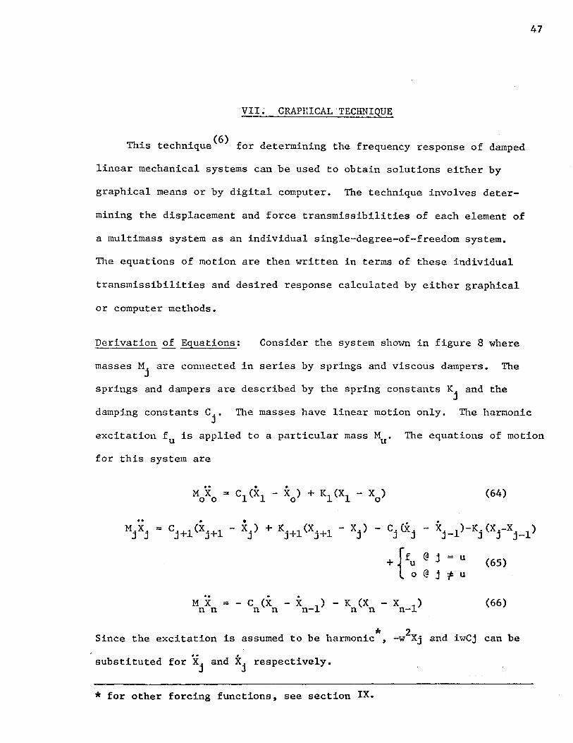
VII~ GRAPHICAL TECHNIQUE
This technique(6
) for determining the frequency response of damped
linear mechanical systems can be used to obtain solutions either by
graphical means or by digital computer. The technique involves deter-
mining the displacement and force transmissibilities of each element of
a multimass system as an individual single-degree-of-freedom system.
TI1e equations of motion are then written in terms of these individual
transmissibilities and desired response calculated by either graphical
or computer methods.
Derivation of Equations: Consider the system sho'tvn in figure 8 where
The masses Mj are connected in series by springs and viscous dampers.
springs and dampers are described by the spring constants Kj and the
47
damping constants Cj. The masses have linear motion only. The harmonic
excitation fu is applied to a particular mass Mu. The equations of motion
for this system are
• - x > Kl(Xl- Xo) (64) MX = Cl(Xl + 0 0 0
•• . • Kj+l (xj+l - xj) - cj <Xj - X. 1)-K. (X.-Xj 1) MjXj = cj+l(xj+l - X ) +
j J- J J -
+{f~ @ j = u (65)
@ j "I u
. - X ) - K (X MX = - C (X - X ) (66)
nn n n n-1 n n n-1
Si h i i i d t b h i * 2x· d i Cj b nee t e exc tat on s assume o e armon c , -w J an w can e
substituted for xj and xj respectively.
* for other forcing functions, see section IX.

48
Figure 8
Damped Nulti-degree-of-freedom System

49
The above equations yield the following subsidiary equations:
(67)
-(iCjw+Kj) Xj-l +(-Mjw2+iCjw+Kj + iCj+lw+Kj+l) Xj
-(iC.+lw+Kj+l) X.+l = {fu@ j=u J J 0 @ j~u (68)
(-M w2+iC w+K ) X -(iC w+K ) X = 0 n n n n n n n-1 (69)
Considering each element as a single-degree-of-freedom system, define
iwCj+Kj l+i2bj w
Tdj = = Woj -M.w2+iwC.+K. l-(~) 2+i2b ..!:'!_ J J J
woj j woj
(70)
-M w 2 -(~)2 w.
Tf. j 0
-MjwZ+iC.w+K. = J 1-(3_.) 2+i2b w
J J w . j w OJ oj
(71)
where (~)~ w. = OJ ~
bj = cj
2(MjKj)~
Tdj is defined as the displacement transmissibility of the individual
element while Tfj is defined as the corresponding force transmissibility.
It should be noted that in most of the textbooks(l,l9), displacement
and force transmissibilities have identical expressions. However, these
have been defined here such that
Tf = l-Td j j (72)

Defining Tfj as above helps in expressing the equations of motion in
terms of these two qualities.
From equations (70) and (71),
(73)
(74)
Substituting these relationships into equations (67), (68), and (69)
(75)
(M.w2 ~ J Tf·
J
X + ( M.w2 M 2 Tdl.+l) X j -1 - 1 - j+lw - j
Tfj Tfj+l (76)
2 Td ( M 1.+1) X - - j+1w - - j+l
Tfj+l
j=U
2 ( 2 Td X (-Mnw y O
- -~w _!l) n-1 + · ) ~"'Il = f Tf T n n
(77)
Dividing equations (75), (76), and (77) through by - w2, the following
equations are obtained:
(M + M Tdl) X - (M Tdl) X = 0 o 1 o 1 Tf 1
Tfl 1
(78)
j = u (79)
j 1: u
50

(80)
TI1e above equations are rearranged to obtain a form that can be
readily adapted to a graphical solution. From equation (78),
or
X I, M Tf1]-l
. X~ =L + M~ Tdl
(81)
From equation (79), three equations are obtained corresponding to
For j < u:
j < u
j = u
and j > u
Let j = 1. From equation (79),
substituting for X from equation (81), 0
(82)
Ml Td2 Td2 + (Tf! + M2 Tf/ Xl -(M2 Tf
2) Xz = O
(83) Equation (83) gives
51

rearranging,
t M1.'l'f2. ·1 + M Tf Td (1
2 1 2
M Td1 X !-
substituting·~ for .... Tfl h b ----- , t e a ove equation reduces to
xl . Td1
Mo + Ml Tfl
[ + :1 ~;2 r! (1 - Td xo~ -1 ~ 2 1 2 l Xl:J
Generalizing the above derivation,
X ~ M Tf Xj-2~-1 _j.=!_ = 1 + _j.=!_ -=.:::.J_ -:-=1=--- (1 - Td . -l X ) X Mj Tdj Tfj-l J j-1
j
For j = u: Equation (79) becomes
(84)
(85)
(86)
f u
- w2
(87)
Dividing through by (X M ) and rearranging, equation (87) yields u u
M X w2
[ X M Td u f~ = _ TTdfuu u-1 + _!_ + u+l u+l
X Tf M Tf +l u u u u
For _j_~: ~-!rite equation (79) as
Mu+l Tdu+1 Xu+l J -1
-~ Tfu+1 x:-(88)
52

Dividing through by Xj+~ and rearranging,
(90)
The above equation is nmv written in the following form:
Xj+l = Td [1 + Mj+2 Tdj+2 (1 Xj+2) J -1 (91) Xj j+l Mj+l Tfj+Z Tfj+l - Xj+l
Lastly, from equation (80),
X n --= Td xn-1 n
(92)
Equations (81), (86), (88), (91), and (92) are used for determining the
system response. The amplitude ratio between the inertia force of
mass j and the external force applied at location u is obtainable by
the relation
M. = _J_
M u
~ X
u
(93)
Similarly, the amplitude ratio between any two displacements is obtain-
able by the relation
~ = X. 2 J-
(94)
53
If the external forces are applied at more than one location, then there
will be an equation similar to equation (88) for each external force.

54
The contribution due to each force can be determined by repeatedly
using equation (93).
To apply the general solution to specific models, several simplifi-
cations can be made. If the input is applied to an end mass, begin the
analysis at the opposite end and progress toward the input. If the
force is applied at each end, the analysis is carried out by taking into
account one force at a time and beginning the analysis at the opposite
end of this force. The net response is obtained by principle of super-
position.
For the case where the first mass is attached to a rigid
M 0
is assumed to be infinite. Then X vanishes and the ratio 0
foundation,
xl -is x2
available as a function of the parameters describing the first and second
elements.
Branc~ed Systems: For the branched system, the transmissibility of
the nodal mass is simply a function of the sum of the branch transmis-
sibilities -the bracketed term in equations (81), (86), (88), (91), and
(92) then has the format 1 +Branch 1 +Branch 2+ •••• To illustrate
the setting up of the equations, consider the system shown in figure 9.
Let n = 3, which is the number of masses in the longest chain, and let
j = 0. Then from equation (92),
x3 Td3
-= x2
(95)
x4 Td
4 -= xl
(96)

J:l
J,;o
7/ll/ll//lll/lll///ll/l//l//
Figure 9
Damped Four-degree-of-freedom System Excited
by Foundation Mot~on
55

From equation (91),
noting Tf4
= l-Td4 , the above equation has the final form
Xl ~ M2 Td2 X2 M4 J -1 -- = Td 1 + - - Tf (1- -) + - Td Tf X
0 1 Ml Tf2 1 x1 Ml 4
. x2 Using equations (97) and (98) g~ves X:'
0
similarly from equations (95) and (99),
and from equations (96)
xo x2
and (98),
x4 x4 xl -=-. xo xl X
0
(97)
(98)
(99)
(100)
(101)
Equat:tons (98) through {101) give the ratio between the amplitude at
any location and the input X0
•
56

57
Note that the rotational motion has been neglected and the masses
are assumed to have translational motion only. (For solving a system
having both rotational and translational motions, see section IX).
Graphical Method for Solution: TI1e graphical solution of equations
(81), (86), (88), (91), and (92) involves the plotting of the individual
transmissibilities Tdj and Tfj. Magnitude and phase angle plots of these
equations are discussed in texts on basic servomechanism theory(ZO).
Magnitudes in decibels are conventionally plotted against frequency
ratio ~ on a semilogarithmic scale. Multiplication is then equivalent woj
to graphical addition. Some of Td and Tf plots(G) of both magnitude
and phase versus frequency ratio are shown in figures 10 and 11. To
proceed with the graphical method, first determine the equations of
motion and evaluate all the known parameters such as masses, damping
ratios, and the undamped natural frequencies of the individual spring-
mass-damper elements. The working curves are based on "uncoupled"
natural frequencies and damping ratios. The appropriate curves of Td
w and Tf versus -- that are required by the specific problem are then Woj
traced onto a sheet of semilog paper. Tile curves representing those
terms that are to be multiplied together are graphically added. If the
solution requires the evaluation of a reciprocal of a function, revolve
the magnitude curve of the function about the 0-decibel line and reverse
the original phase relationship. Mass-ratio terms may be combined with
Tf and Td curves by first determining the decibel value of the mass
ratio and then shifting the associated Tf and Td magnitude curve up or
down by this value. Tile accuracy of the graphical technique is depen-
dent upon the quality of the working curves.

40
tl) 30
...-i a,)
..0 2 •ri 0 a,) ~ lO .. a,)
"0 0 ;:I ~ •ri Q -to 00 Cll
;:E.:
"0 -E:-1
-30
-40
tl) a,) a,) ~ 00 a,) ~
... a,)
...-i 00
~ <I) tl)
Cll .a ~
~
0
-60
-12.0
-180
Frequency Ratio ~ woj
Figure 10.
Td Magnitude and Phase-angle Characteristics
bj:::.l·O
bj~O.S
58
too

.3o
oo Zo r-1
<1.1 ..0 . ..-~ Jo u <1.1 ~
.. 0 <1.1
"0 e -lo •.-I ~
~ -20 ::.=
~ -3
Cll <1.1 <1.1 1-1 00 <1.1 ~ .. Cll <1.1
r-1 00
~ <1.1 Cll ~
..c: P1
4-l ~
180
I20
60
0
w Frequency Ratio, woj
Figure 11
1-0
Tf Nagnitude and Phase-angle Characteristics
59
10·0

Another form of graphical solution consists of vector diagrams
where various vectors can be added or subtracted. Before drawing·
vector diagrams, all multiplications and divisions are carried out by
algebraic methods and the final expression is reduced to a form which
contains additions and subtractions of vectors only.
To illustrate this procedure, consider equation (85):
1 (85)
xl It is desired to obtain the magnitude and the phase angle of X: .
2 For
M1 Tf2 1 M1 Tf2 Td1 X0 this, first evaluate the products M
2 Tfl Td
2 and M
2 Tfl Td
2 x
1• The
two vectors thus obtained are then added in a vector diagram. Add
vectorially 1 to the resultant vector. This gives the denominator of
xl the right-hand side of the above equation. The expression for X
2 is
reduced to the form
1 -x-
2 = -A-L-:-t:-
where A is the magnitude of the denominator and S is the phase angle.
xl now become x2
which is the desired result.
Either of these graphical methods may be employed depending upon
the individual's preference for solvi~g a particular problem. There
appears to be no specific advantage of one method over the other.
60

61
With a relatively small amount of labor and considerable saving of
time, one can solve multimass transmissibility problems by the graphical
technique without solving mathematically the equations of motion.
62
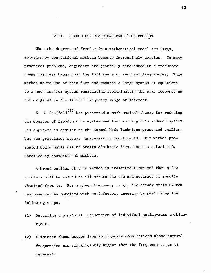
VIII. METHOD FOR REDUCING DEGREES-OF-FREEDOM
When the degrees of freedom in a mathematical model are large,
solution by conventional methods becomes increasingly complex. In many
practical problems, engineers are generally interested in a frequency
range far less broad than the full range of resonant frequencies. This
ntethod makes use of this fact and reduces a large system of equations
to a much smaller system reproducing approximately the same response as
the original in the limited frequency range of interest.
s. E. Staffeld(]) has presented a mathematical theory for reducing
the degrees of freedom of a system and then solving this reduced system.
His approach is similar to the Normal Mode Technique presented earlier,
but the procedures appear unnecessarily complicated. The method pre
sented below makes use of Staffeld's basic ideas but the solution is
obtained by conventional methods.
A broad outline of this method is presented first and then a few
problems will be solved to illustrate the use and accuracy of results
obtained from it. For a given frequency range, the steady state system
response can be obtained with satisfactory accuracy by perfornting the
following steps:
(1) Determine the natural frequencies of individual spring-mass combina
tions.
(2) Eliminate those masses from spring-mass combinations whose natural
frequencies are significantly higher than the frequency range of
interest.

63
(3) Solve the reduced system for its steady state response by any of
the conventional methods.
Step (2) is reasonable because: (1) the lowest system eigenvalue
is less than the lowest frequency of any individual spring-mass combin-
ation, (2) the eigenvalues of the system which are greater than the
frequency range of interest are due to those masses whose individual
spring-mass combination frequencies are higher than the frequency range
of interest. Therefore, elimination of these masses from the system has
little effect on system response within the frequency range of interest.
The elimination of the masses whose individual spring-mass frequencies
are closer to the operating frequency depends upon individual judgement.
Witl1 experience, it should be possible to eliminate the masses whose
omission from. the system does not produce a large error in the system
response.
Elimination of some of the masses automatically reduces the degrees
of freedom. However, the effect of these masses in the frequency range
of interest is included by altering the spring constants associated with
the original spring-mass combinations. These are altered to account for
the inertia force produced by the missing masses. The original spring
2 constant K is replaced by K-mw0 , where w0
is the usual (or typical)
operating frequency. The system modified as above will have exactly
the same behavior as the original system at w and will generally be a 0
good approximation to it in the neighborhood of w0 •

64
If the mass to·be eliminated happens to be the outermost mass, then
* the spring attached to this mass is assumed to have infinite stiffness •
This permits coupling of this mass with the one which precedes it.
If viscous damping is present, it is assumed that the normal modes
not in the frequency range of interest may be represented by modified
springs without mass and damper. The resulting reduced damped system
equations are then solved by one of the methods presented previously,
for the remaining eigenvalues and eigenvectors.
The potential savings in work arises from two sources:
(1) All of the eigenvalues and eigenvectors need not be found.
(2) Fewer forced vibration equations are required and the uncoupling
procedure is thereby simplified.
Illustrative Examples: As a first example, consider the system shown
in figure 12 with
2 M
1 = M
2 = M3 = 1 lb-sec /in.
K1
= 100 lbs/in., K2 = 4 lbs/in., K3 = 1 lb/in.
Operating frequency range = 0 to 3 rad/sec.
It is required to find natural frequencies in the operating fre-
quency range and the corresponding amplitudes of the masses.
* See illustrative example on page 67.

65
.LL.Cli.~-:LL.:.C. JVJ4 :::::: 00
x4- =- o
Figure 12
A Spring-Mass System

Solution: The actual solution is presented first. For this, any of
the conventional methods can be used; the tabular method of Holzer has
been employed here. The boundary condition for this problem is x4 = 0
at all times. Holzer tables for the three natural frequencies are
given below:
Holzer Table for First Natural Frequency
'r::1hl~=> T• t,l - 0 1()
Mass M Mw2 xi
2 IHw2Xi Ki,i+l
IMw~Xi Mw xi ---
No Ki,i+l
1 1 .3 1.0 .3 .3 100 .003
2 1 .3 .997 .297 .597 4 .149
3 1 .3 .848 .254 .851 1 .851
4 00 -.003
The amplitude of the first mass is arbitrarily taken as one unit.
2 For w = .3, x4 = -.003 ~ 0. This shows that the trial frequency is
natural frequency of the system and since only one sign change in the
* amplitude column occurs, there are no natural frequencies below this •
Therefore, w1
= ~ = 0.548 rad/sec.
* For a detailed explanation, refer to Holzer's Method on
page 27.
66

Holzer Table for Second Natural Frequency
Table II: 2 = 6.64 w
Mass M Mw2
xi 2
LMW2Xi .rMw2xi
No Mw xi Ki,i+l
Ki,i+l
1 1 6.64 1.0 6.64 6.64 100 .0664
2 1 6.64 .9336 6.195 12.835 4 3.209
3 1 6.64 -2.2754 15.11 -2.275 1 -2.275
4 00 -.0004
w2 = 16.64 = 2.582 rad/sec
A similar table gives the third natural frequency w3 = 14.28 rad/sec.
Reduced System: Individual natural frequencies are
w1 = Jfi = ~ = 10 rad/sec
w2 = ~~~- Ji = 2 rad/sec
w = Pi:= ~~ = 1 rad/sec 3 M3
Since the operating frequency range is 0 to 3 rad/sec, w1 lies outside
the frequency range of interest. Therefore mass M1 can be eliminated.
Since M1
is outermost mass, dropping M1 results in omission of K1 also.
67
To take care of such situations, K1 is assumed to have infinite stiffness.
TI1is enables M1
to be added to M2 and the reduced system is represented
as

Figure 13. Reduced Spring-Mass System
In other words, it is assumed that the amplitude of M1
is the
same as tl1at of M2 • This assumption is supported by the actual dis
placements of M1 and M2 as observed from Holzer tables for first and
second natural frequencies.
Holzer tables for the reduced system are as follows:
Table I: 2 - n .~ w
Mw2 2 LMw2Xi Ki,i+l
LHw~Xi Mass M xi Hw xi Ki,i+l No
1 2 .6 1 .6 .6 4 .15
2 1 .3 .85 .255 .855 1 .855
3 00 -.005
wl "' 1:3 = .548 rad/sec
68

Table II: 2 = 6.7 w
Mass M Mw2
xi 2
}:Mw2
Xi XMw2Xi
No Mw xi Ki,i+l
Ki,i+l
1 2 13.4 1.0 13.4 13.4 4 3.35
2 1 6.7 -2.35 -15.75 -2.35 1 -2.35
3 00 0
w2 = ~ = 2.588 rad/sec
A table comparing the actual and reduced system solutions is presented
below. For this table, x1 and x2 represent vectors consisting of
amplitudes of only those masses whose individual eigenvalues lie within
frequency range of interest. These are obtained from the amplitude
columns associated with the first and second natural frequencies.
Comparison of Actual and Reduced Systems
wl w2 xl x2
Actual solution .548 2.582 11.0}* { 1.0]* .85 -2.4
Reduced System Solution .548 2.588 {.~5} { -2~ 35}
It can be seen from the above table that eigenvalues in the frequency
range of interest obtained by this method compare closely with the
actual eigenvalues. Also the displacements given by this method do not
vary significantly from actual displacements of the original system.
* Note that the amplitude of the mass M2 has been scaled to 1.
69

70
As a second example, consider the system shown below, where the mass
to be eliminated happens to be other than the outermost mass.
xt.T Figure 14. A Spring-Mass System
Given data: ------
K1
= 1 lb/in., K2 = 5 lb/in., K3 = 10 lb/in.
Usual operating frequency = 2 rad/sec.
It is required to find eigenvalues and the corresponding eigenvectors
in the neighborhood of the operating frequency.

71
Actual Solution: (Holzer's Hethod)
Table I: 2 = 0.71 w
Mass M Mw2 xi
2 LMw2Xi
.· .XHw2xi
No/ Mw xi Ki,i+l Ki,i+1
1 1 .71 1.0 .71 .71 1 .71
2 1 .71 .29 .206 .916 .5 .183
3 1 .71 .107 .076 .992 10 .0992
4 00 .008
wl "" r.n = .8425 rad/sec
Table II: 2 = 4.05 w
Mass M Mw2 xi
2 IMw2Xi Ki,i+l
IMw2Xi Mw X.
Ki,i+1 No ~
1 1 4.05 1.0 4.05 4.05 1 4.05
2 1 4.05 -3.05 -12.35 -8.3 5 -1.66
3 1 4.05 -1.39 -5.64 -13.94 10 -1.394
4 00 +.004
w2 "" 2.013 rad/sec
And the third natural frequency w3 is found to be 4.15 rad/sec.
Reduced System: The individual spring-mass combination frequencies
are
wl = 1.0 rad/sec
w2 = 2.27 rad/sec
w3 = 3.17 rad/sec

which indicates that M3 can be eliminated. The effect of elimination
of M3 is included by modifying K3
as follows:
2 modified stiffness K = K3
- M3w
0
where w is used usual operating frequency. 0
K = 10- (1)(4)
= 6 lb/in.
The Holzer tables for Reduced System are given below:
Table I: 2 w = .675
Mw2 2 }:Mw
2Xi Ki,i+l
}:Mw2Xi
Mass M xi Mw xi Ki,i+l No
1 1 .675 1 .675 .675 1 .675
2 1 .675 .325 .219 .894 2.73 .327
3 00 -.002
wl "" .822 rad/sec.
Table II: 2 = 4.05 w
2
Mw2 2 }:Mw
2Xi
}:Mw xi Mass M xi Mw xi Ki,i+l Ki,i+l No
1 1 4.05 1.0 4.05 4.05. 1 4.05
2 1 4.05 -3.05 -12.35 -8.3 2.73 -3.04
3 00 -.01
w2 =:! 2.013 rad/sec.
72

73
The reduced system for the second illustrative example is
K=-6
Figure 15
Reduced Spring-Mass System
which is equivalent to
Figure 16
Equivalent Reduced System
K K2K 5X6 - 2 73 lb/in. eq = K
2+K = 5+6 - •

74
A comparison of results obtained by actual and reduced system solutions
is presented below:
Comparison of Actual and Reduced Systems
wl w2 xl x2
Actual solution .8425 2.013 {.~9} {-~.os} r--
Reduced system solution .822 2.013 {.;2~ { _;_os}
It can be seen from above two examples that approximating a system
can reduce the degrees of freedom and at the same time give results
which compare well with the actual solution. With a little experience,
this method can save a considerable amount of labor when a large num-
ber of degrees of freedom is involved.

IX. SUMMARY AND CONCLUSIONS
In this work various methods for the analysis of linear damped
multi-mass systems have been studied. Naturally, a question arises as
to the suitability of these methods for solution of a specific problem.
Any comparison between these methods should be based on the following
points:
(1) The amount of labor and time required to formulate a mathematical
model and to obtain the natural frequencies and system response.
(2) The approximations involved and consequently the accuracy of
results.
(3) Application to systems such as (a) those with masses and dampers
connected to a reference frame; and (b) those having both linear and
angular motions.
(4) Ease of application when used (a) manually; or (b) with a digital
or analog computer.
The advantages and disadvantages of each of the methods presented
earlier will now be discussed on the basis of the above points.
~ormal Mode Technique:
(1) Even for systems with many degrees of freedom the derivation of
75
the equations of motion is straightforward and does not present any
problem. However, when the degrees of freedom are large, required
operations involving the mass, stiffness, and damping matrices can be
laborious. If the system is classically damped, the natural frequencies

76
and the system response can be obtained without great difficulty.
However, non-classically damped systems are extremely difficult to
solve even for as few as three degrees of freedom, as is illustrated
by the sample problem in Appendix D. Another major disadvantage of
this method lies in the fact that to ascertain the nature of the system
(whether classically or non-classically damped), M, K, and C matrices
have to be obtained. This requires the derivation of the equations of
motion as a first step. If it is discovered that the system is non-
classically damped, any of the other methods may be more desirable to
employ.
* (2) The results obtained by this method will always be exact ,
since there are no approximations involved.
* (3) This method provides the solution to any kind of system •
If there are combined linear and angular motions, the degrees of free-
dom will be more than the number of masses and consequently there will
be additional equations of motion. However, a complete solution is
** mathematically possible, with two exceptions (1) when there are
less than 2N independent eigenvectors in the case of repeated roots of
the frequency equation of non-classically damped systems; (2) when one
or more of the free vibrational modes is critically damped.
* These comments apply to only linear systems.
** Note that these conditions rarely occur in practice.

77
Of the five methods discussed, this is the only method which
provides th~ system transient response. Though not the topic of this
thesis, this is an advantage of the Normal Mode Technique over the other
methods.
(4) For classically damped systems having more than two or three
degrees of freedom, obtaining the solution by the Normal Mode Technique
can be time-consuming if manually done. Therefore, use of a digital
computer is recommended for systems having more than 3 degrees of freedom.
For non-classically damped systems, use of a computer is essential.
Holzer's Method:
(1) This method does not make use of the frequency equation. The
eigenvalues and system response are obtained by trial and error without
deriving the equations of motion. This is one of the principal advan
tages of this method. Another significant advantage is that the higher
eigenvalues can be obtained as easily and with as much accuracy as the
fundamental eigenvalue. The eigenvectors are directly obtained from
the amplitude column of the Holzer table without additional effort.
Also, Holzer's Method is ideal for obtaining steady state system response
to external harmonic inputs. Only one table needs to be constructed
for the impressed frequency; no trial and error procedure is involved.
The disadvantage of this method is that a trial and error method
is required for determining the eigenvalues; this can be a difficult
task if the system has more than a few masses or if damping is present.

(2) Since a trial and error procedure is involved, some accuracy
may have to be sacrificed unless a digital computer is employed. How-
ever, use of a computer should permit any practical degree of accuracy
to be attained in a reasonable time.
(3) Holzer's Method can be employed to solve systems with dampers
connected either between two masses or between a mass and the reference
78
frame, as shown in section V. However, systems having coupled rotational
and translational motions have not been treated by this method. In this
case the mass has a combination of inertia force and inertia torque
which makes the problem quite complex and beyond the scope of this work.
Another application of Holzer's Method is in the study of transverse
vibrations of beams. When a beam is replaced by lumped masses connected
by massless beam sections, a modification of Holzer's Method can be
used to compute progressively the deflection, slope, moment, and shear
from one station to the next. This method has been developed by N. 0.
(1 23) Myklestad and M. A. Prohl ' .•
(4) When the degrees of freedom are four or less, computations·
can be performed manually without great difficulty. However, for large
systems, use of a computer can result in substantial savings of time
and labor.
Impedance Method:
(1) The formulation of the equations which describe system performance
by the Impedance Method is relatively simple. It does not require deri-
vation of the equations of motion. At the same time, neither the

natural frequencies nor the mode shapes can be obtained directly from
this method, which may be a major disadvantage. A second disadvantage
79
of the Impedance Method is that it requires solution of numerous simul
taneous equations to obtain the desired relationship between input and
output quantities. This can be a laborious task. However, compared to
the Normal Mode Technique, this method is much simpler to use for steady
state forced vibrations.
(2) There are no approximations involved and therefore this method
is exact for harmonic inputs.
(3) The method is applicable to a very large class of systems.
The only practical exception is a system with coupled linear and angular
motions. In this case it may be difficult to determine and use the
four-pole parameters for the various system elements.
(4) Nost of the computations for this method are relatively simple
to perform and do not require the use of a digital computer. Hmvever,
some experience in combining the simultaneous system perfonnance equa
tions can result in considerable savings of time.
Graphical Technique:
(1) Derivation of the equations of motion and expressing these in a
form which is suitable for plotting comprises the major part of the
work for this method. The eigenvalues cannot be found directly by this
technique. However, some estimation of natural frequencies can be
obtained by determining system responses for various harmonic input
frequencies. The peaks in the plot of the output magnitude versus fre-

quency closely correspond to the natural frequencies of the system.
The system response is relatively easy to obtain once the equations
are expressed in proper format.
(2) The results obtained by this method are not, in general, as
accurate as those obtained from other methods. The accuracy depends
to a large extent upon the quality of the working curves.
80
(3) This technique is ideally suited for systems with masses
connected by dampers and springs and having no other elements. Dampers
connecting masses to the reference frame can be handled by this method
but complicated equations often result. Therefore, Holzer's Method is
recommended in this case. The Graphical Method cannot be applied directly
to problems having coupled linear and angular motions, because the com
posite transmissibilities are not defined in this case.
(4) Since the solution is obtained by graphical means, all of the
work has to be done manually. However, each stage of the graphical
solution can be computerized for improved accuracy.
Reduced System:
Once the original system is reduced to a new system of fewer degrees of
freedom, it can be solved by any one of the conventional methods. While
the procedure for reducing the degrees of freedom is a simple one, con
siderable experience may be required to eliminate only those masses and
dampers whose presence has little effect in the frequency range of
interest.

As is obvious, this is an approximate method. It can be useful,
however, when the degrees of freedom of a system are large. Finding
81
the responses of such systems may tax the capacity of a digital computer.
Reducing the degrees of freedom of such systems often helps in handling
these systems mathematically, without significant loss of accuracy.
For undamped systems, results obtained by this method agree closely
with the actual solutions. The accuracy of this method when applied to
damped systems will depend upon the accuracy of the conventional method
employed to solve the reduced system.
It should be mentioned here that the inputs considered for obtaining
tl1e steady state response are sinusoidal in nature. To obtain the res
ponse for other types of inputs, several methods(2
) are available such
as Fourier Series Expansion, Laplace Transformation, etc.
It is thus concluded that all of the methods presented in this
thesis can produce accurate results if an appropriate method is selected.
This su~~ary is intended to serve as a guide for selection of the method
best suited to the solution of a particular problem.

X. SUGGESTIONS FOR FURTHER WORK
There is little need to stress the desirability of attempting to
evaluate further some of the methods presented in this thesis. A few
suggestions for further work are:
(1) A systematic procedure for solving systems with coupled angular and
linear motions by Holzer's Method, the Impedance Method, and the Graphi
cal Technique needs to be developed.
(2) Several classes of systems need to be analyzed by the Graphical
Technique and the Reduced System Method to ascertain the applicability
as well as the accuracy of these methods.
82
(3) Further work and experience in solving systems by reducing the
degrees of freedom should permit development of a standard procedure for
eliminating only those masses which have little effect on system behavior
in the frequency range of interest.
(4) An approximate solution by the Normal Mode Technique can be obtained
by ignoring off-diagonal terms of the damping matrix, but the results
may be inaccurate. A method should be developed to include, in an optimum
manner, the effect of the off-diagonal terms by altering the diagonal
elements of the damping matrix.

BIBLIOGRAPHY
1. Thompson, W. T., (1965) "Vibration Theory and Applications". N. J., Prentice Hall Inc., p. 159-251.
2. Anderson, R. A., (1967) "Fundamentals of Vibrations". New York, Macmillan, p. 157-246.
3. Tse, Horse, Hinkle, (1966) "Mechanical Vibrations". Boston, Allyn and Bacon, p. 229-263.
4. Den Hartog, J. P., (1956) "Mechanical Vibrations". New York, HcGraw-Hill, p. 122-130.
5. Holloy, C. T., (1957) "Use of Four-pole Parameters in Vibration Calculations". Jour. Acous. Soc. Amer., p. 842-853.
6. Pechter, Kamei, Tanner, Knudsen, (1965) "Technique for Determining the Frequency Response of Linear Hechanical Systems". Jour •. Acous. Soc. Amer., p. 66-76.
83
7. Staffeld, S. E., (1962) "A Hethod for Reducing the Number of Degrees of Freedom in Hathematical Models of Damped Linear Dynamic Systems". Journal of Engineering for Industry, Trans. ASHE, p. 418-422.
8. Eddy, E. H., (1965) "Digital Computer Applied to Analysis of Damped Hultimass Torsional Vibration System". Quarterly Journal of General Motors, 2nd quarter, p. 27-33.
9. Den Hartog, J. P., (1956) "Mechanical Vibrations". New York, McGra\v-Hill, p. 187-193.
10. Den Hartog, J. P., Li, L. P., (1946) "Forced Torsional Vibrations \-lith Damping: An Extension of Holzer's Hethod". Trans. ASHE, p. A276-280.
11. Foss, K. A., (1958) "Coordinates Hhich Uncouple Hotion of Damped Linear Dynamic Systems". p. 361-364.
the Equations of Jour. !E.£_. Mech.,
12. Caughey, T. K., (1960) "Classical Normal Modes in Damped Linear Dynamic Systems". Jour. ~· Hech., p. 269-271.
13. O'Kelly, H. E. J., (1961) "Normal Hodes in Damped Systems". Pasadena, California.Thesis, California Institute of Technology, p. 179.·

14. Greenwood, D. T., (1965) "Principles of Dynamics". N. J., Prentice-Hall, p. 229-258.
15. Hohn, F. E., (1964) "Elementary Matrix Algebra". New York, Macmillan, p. 336-340.
16. • Same as ref. (15). p. 294-298 •
17. • Same as ref. (15). p. 273-276.
18. Gere, J. M., Weaver, W. Jr., (1965) "Matrix Algebra for Engineers". N. J., Van Nostrand, p. 109-126.
19. Church, A. H., (1963) "Mechanical Vibrations". New York, John Wiley, p. 138-143.
20. ·Raven, F. H., (1961) "Automatic Control Engineering". New York, McGraw-Hill, p. 150-163.
21. Tse, Morse, Hinkle, (1966) "Mechanical Vibrations". Boston, Allyn and Bacon, p. 131-133.
22. Church, A. H., (1963) "Mechanical Vibrations". New York, John Wiley, p. 303-324.
23. Vierck, R. K., (1967) "Vibration Analysis". Scranton, Pa., International Textbook, p. 258-263.
84

85
APPENDICES

86
APPENDIX A
Reciprocity Theorem
Maxwell's reciprocity theorem will be proved(2l) here for influence
coefficients. An influence coefficient oij is defined as the static
deflection of the system at station i owing to a unit force applied at
station j of the system. Thus, by definition, oij is reciprocal of Kij"
To prove the theorem, consider the simply supported beam of figure 17
in which two vertical forces F1 and F2 are applied at stations 1 and 2.
For this illustration, the influence coefficients are o11 , o12 , o21 , and
o22
• The deflection at station 1 owing to the force F2 applied at station
2 is F2o12
•
Assume that the procedure of loading is separated into two steps.
First, F1
is applied to station 1 and then the force F2 is applied to
station 2. When F1
is applied alone, the potential energy in the beam
1 2 by virtue of its deformation, is equal to 2 F1 o11• Now, when F2 is
applied, the additional deflection at station 1 owing to the force F2 is
F2
o12
• T11e work done by F1
corresponding to this deflection is F1 (F2o12).
Hence the total potential energy in the system is
The last two terms of this equation represent the additional potential
energy which is due to the application of F2 •
Second, F2
is applied to station 2 and then the force F1 is applied
to station 1. The potential energy of the system is

87
Fz
1
- -t_ - - --· _..
Figure 17
A Simply Supported Beam \-lith Two Loads

The last two terms of this equation are due to the application of
Fl.
88
Since the final states of the system are identical for the two
methods of loading, by the law of conservation of energy, the potential
energies expressed in the two cases are the same. By equating the two
expressions for potential energy, it is deduced that o12 = o21 •
Generalizing the above proof for several loads, we have
oij = oji
Since oij is the reciprocal of Kij' it follows that Kij = Kji.
On the same lines, it can be proved that
cij = cji
The above relationships hold for any linear system.

APPENDIX B
Review of Matrix Operations
There are many properties and relationships that pertain to the
eigenvalues and eigenvectors of a square matrix(lS), and those that
are useful in vibration problems will be mentioned here.
(1) The eigenvalues of a real symmetric matrix are always real
and consequently the eigenvectors of such a matrix are also real. This
is true because in this case all the coefficients in the characteristic
equation are real(l6).
(2) All eigenvectors associated with distinct eigenvalues will
be linearly independent(l7). Furthermore, the eigenvectors are fre-
quently linearly independent even when there are repeated eigenvalues.
For a symmetric matrix of order n, n linearly independent eigenvectors
will always exist even though the eigenvalues may be repeated.
(3) All of the eigenvectors of a symmetric matrix are orthogonal
to one another. To prove this, consider two different eigenvalues Ei
89
and Ej of a symmetric matrix A. TI1ese eigenvalues satisfy the equations
(1)
(2)
in which Xi and Xj are the eigenvectors associated with Ei and Ej
T respectively. Premultiplying equation (1) by Xj (transpose of the
T colutnn vector X ) and equation (2) by x1 ,
j .

90
(3)
(4)
Taking the transposes of equations (3) and (4) yields two more equations
(5)
(6)
The left-hand sides of equations (3) and (6) are the same, and similarly
for equations (4) and (5), the right-hand sides of these equations may
be equated. Thus,
Rearranging these equations gives
Because Ei and Ej are assumed to be different eigenvalues, it follows
from equation (7) that
which shows that the eigenvectors Xi and Xj are orthogonal vectors.
(18) By a more involved analysis , the same results can be confirmed for
eigenvectors that are associated with repeated eigenvalues. Thus, the
important conclusion is obtained that all of the eigenvectors of a
symmetric matrix are orthogonal to one another.

91
The above orthogonality condition applies when the matrix product
of (M]-l LK] is symmetric. For the case when [M)1 [K) is not symmetric,
the following orthogonality conditions for the normal modes exist:
For the ith normal mode,
(8)
Similarly, for the jth normal mode,
(9)
Premultiplying equations (8) and (9) by the transposes of the jth and
ith modal columns respectively, we can write
{qj}T(K){qi} = wi2{qj}T(M){qi}
. {qi}T(K){qj} = wj2{qi}T(M){qj}
(10)
(11)
taking the transpose of both sides of equation (10) and noting that
both (M] and [KJ are symmetric matrices, we obtain
(12)
Subtracting equation (12) from equation (11),
(13)
From above equation, it can be concluded that for distinct eigenvalues,
(14)
Similarly, it can be shown that for 'tvi-:f=. '~j,
(15)

92
Equations (14) and (15) are the orthogonality conditions for the normal
modes. If there are repeated eigenvalues, each of the associated normal
modes will be orthogonal to any normal mode associated with a different
eigenvalue(2).
(4) Any square matrix of order nxn can be diagonalized(l6)
(transformation of a matrix to a diagonal matrix) provided that the
matrix has n linearly independent eigenvectors.
The following example will exhibit some of the above properties:
Let LBJ = ~78 150
200
TI1e eigenvalues of this matrix are
E = 3 1
-60 1~ -117 30
-160 43
Because two of the eiganvalues are the same and the matrix is unsym
metric, it is not clear at this point whether or not [B] can be dia-
gonalized. However, for the repeated eigenvalue E = 3, the solution
of the resulting homogeneous equations has two linearly independent
solutions:
That the above solutions are linearly independent can be verified from
the fact that the vector x1 cannot be expressed as a linear combination
of vector x2
• Since the vectors are linearly independent, the matrix
can be diagonalized. The third eigenvalue gives an eigenvector equal to

93
x3 = B3m
Letting B1 = B2 = B3 = 1, the modal matrix Q, the columns of which are
vectors x1, x2, and x3
, become
-[ 4 -1
:J [Q] 5 0
0 5
[ 30 -23
-~ (Ql-1 = ~ 40 -32
-25 20
and
(<ifl (B] [Q) =[ -~J 3 0
0 3 = [n] 0 0
\vhere (D]is a diagonal matrix the elements of which are eigenvalues
of the original matrix.
From the above example, it is clear that the eigenvectors associated
with repeated eigenvalues of an unsymmetric matrix are not necessarily
orthogonal to one another (as can be observed from vectors x1 and x3
Some definitions pertaining to a symmetric matrix which have been
used in Section (IV), will be mentioned here(l5).
A symmetric matrix is said to be Positive Definit~ if all of its
eigenvalues are positive.

94
If all eigenvalues are positive and at least one is zero, the matrix
is Positive Semidefinite.
A matrix that may be either Positive Semidefinite or Positive
Definite is called Nonnegative Definite.

APPENDIX C Parallel Four~pole Networks
To derive the formulas for a parallel four-pole network, we have
Solving the above equations simultaneously for v i 2 g ves,
From equations (1) and (3),
Fl ( All Vl
F2 = All -~11 A22
(1)
(2)
(3)
(4)
It should be observed that for individual four-pole parameters of mass,
spring, and damper, the following relationship holds(S):
= 1 (5)
The physical significance of this relationship is that these elements
obey the reciprocity principle. However, the above relationship is not
95
necessarily true for all systems which follow the reciprocity principle.
Equations (1) through (5) are written for the spring and damper
individually. The total force carried by the spring and the damper is
then equated to the force at the input or at the output point. The
desired relationships can then be obtained after solving some simultaneous
equations.

APPENDIX D
Sample.Problem:
Often practicing engineers experience considerable difficulty
in deciding upon a method for solution of vibration problems. Appro
priate selection of a method can result in great savings of time and
labor without sacrifice of accuracy. A problem is presented below to
illustrate this point and also to demonstrate the use of the math
ematical theory presented. For this purpose, the system shown in
figure 18 is selected. This system is an approximation of a vehicle
driven on a rough road. It is assumed that (1) the vehicle is con
strained to three degrees of freedom in the vertical direction and
the rotational motion of any of the masses does not occur; and (2) the
tires do not leave the road surface*.
In figure 18, M1 represents the mass of passengers in the vehicle;
M2 is the sprung mass of the vehicle and M3 is the unsprung mass of
the tire assembly. The values of the springs and the dampers between
the masses are reasonable approximations of the physical system. The
vehicle fonvard speed is 20 mph, and the road surface varies sinusoid
ally with a period of 10.5 ft. and an amplitude X0
of 2.0 in ••
It is desired to obtain the undamped natural frequencies and the
mode shapes, as well as the response of the system to the hannonic
excitation, by the methods presented earlier. The results will then
be compared.
*This assumption permits a continuous displacement input to the system.
96

Ml = M = 386 lbs Kl = K = 150 lb/in. cl = c = 17.13 lb/in./sec
M2 = 10M K2 = SK c2 = 7C
M3 = l.SM K3 = 25K c3 = 9C
1-<z c2.
M5 J:l
~) (.3
X:=. Xo ·Sin wl:
Figure 18
A Damped TI1ree Degree-of-freedom System
Excited by Foundation Motion
97

Solution:
Speed = 20 mph = 28.8 fps.
The excitation frequency is
w . 28.8
= 10.5 = = 17.2 rad/sec 2.74 cps
Normal Hode Technique:
Applying Newton's law of motion, the equations of motion of the
system are obtained as
where F is a complex number and is given by 0
F 0
=
The equations of motion in the matrix form can be expressed as
. M1 0 0 cl -cl 0 xl Kl -Kl 0 xl .. . 0 M2 0 + -C 1 Cl+C2 -c 2 x2 + -Kl Kl+K2 -K2 x2
• 0 0 M 0 -c
2 x3 0 -K 2 K2+K x3
0
0
F
(1)
(2)
(3)
(4)
0
(5)
Substituting the values of masses, damping coefficients and spring
constants in equation (5),
98
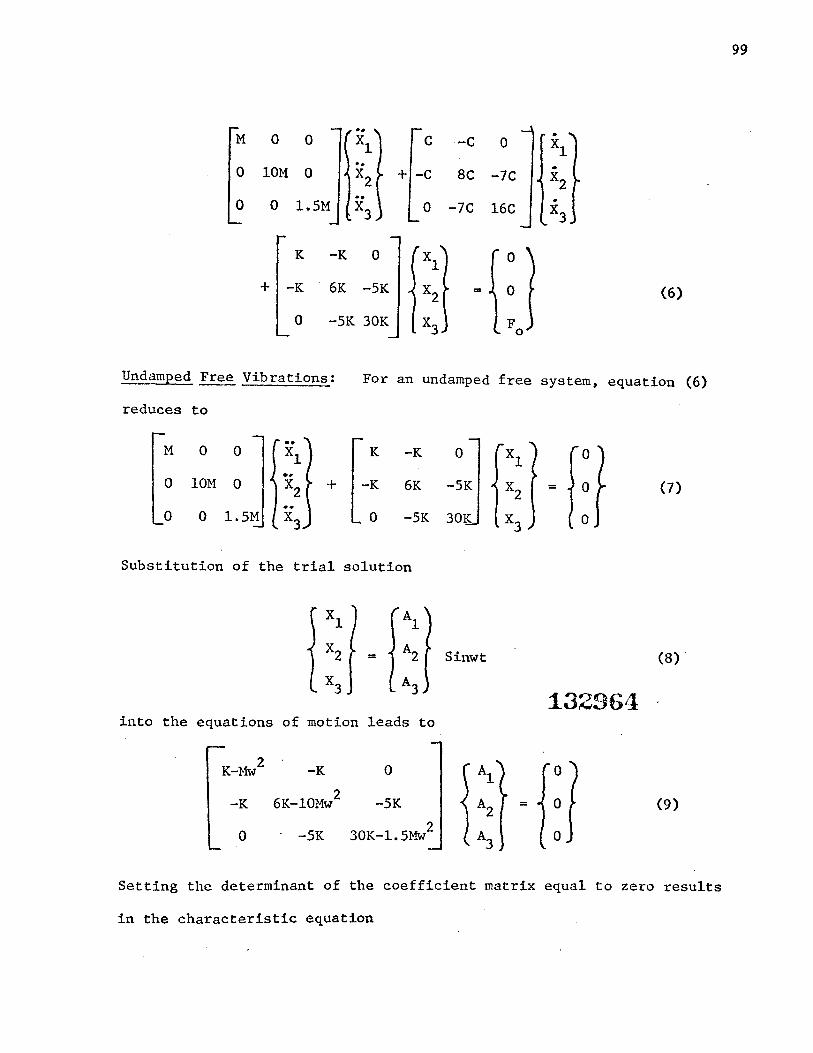
.. . M 0 0 xl c -c 0 xl .. . 0 10M 0 x2 + -c 8C -7C x2 .. . 0 0 l.SM x3 0 -7C 16C x3
K -K 0 xl 0
+ -K 6K -SK x2 = 0 (6)
0 -SK 30K x3 Fo
Undamped Free Vibrations: For an undamped free system, equation (6)
reduces to
M 0 0 K -K ..
0 lOH 0 X2 + -K 6K
0 0 -SK
Substitution of the trial solution
into the equations of motion leads to
2 K-Hw
-K
0
0
-SK
-SK 30K-1.5Mw2
0
= 0 (7)
0
Sinwt (8)
0
= 0 (9}
0
Setting the determinant of the coefficient matrix equal to zero results
in the characteristic equation
99

6 K 4 . K2 2 w - 21.6 M T,v + 31.0 2 w
M
which yields the three eigenvalues
2 .K wl = 0.363 M
2 K w2 = 1.17 M
2 K w3 = 20.1 M
Substituting forK and Min equation (11),
w1 = 7.38 rad/sec
w2 = 13.25 rad/sec
w = 54.9 rad/sec 3
K3 8.34 M3" = 0 (10)
(11)
To obtain the eigenvectors, substitute the first eigenvalue in equation
(9)' .
.637K
-K
0
-K 0
2.37K -5K
-5K 29.45K
Therefore, the homogeneous equations to be solved are
.637 A1 - A2 = 0
-A1 + 2.37 A2-5 A3 = 0
-5 A2 + 29.45 A3 = 0
Setting arbitrarily the amplitude of the first mass to unity, the mode
shape at the first natural frequency is
100

{
1.0} x1 = .637
.108
Repeating the above procedure for the remaining eigenvalues, the cor-
responding mode shapes are
{
1.0} x2 = -.17
-.032 {
1.0} x3 = -19.1
760
The modal matrix whose columns are the vectors x1 , x2
, and x3
, becomes
[
1.0 1.0
'[Q] = 637 -.17
108 -.032
1
-19.1
760
101
Forced Vibrations With Damping: To obtain the response to the harmonic
excitation, we first determine whether the system is classically or
non-classically damped. Thus,
5.067M
0
0
[QJT [c) [Ql = c ~:~~: ~2140
0
!.29M
0
0
1.45K
0
-.72
1.263
575
=[M)
= (K J
-2130d 555
9.45xl0
It is observed from the above matrices that the transformation which
diagonalizes the M and K matrices does not diagonalize the damping
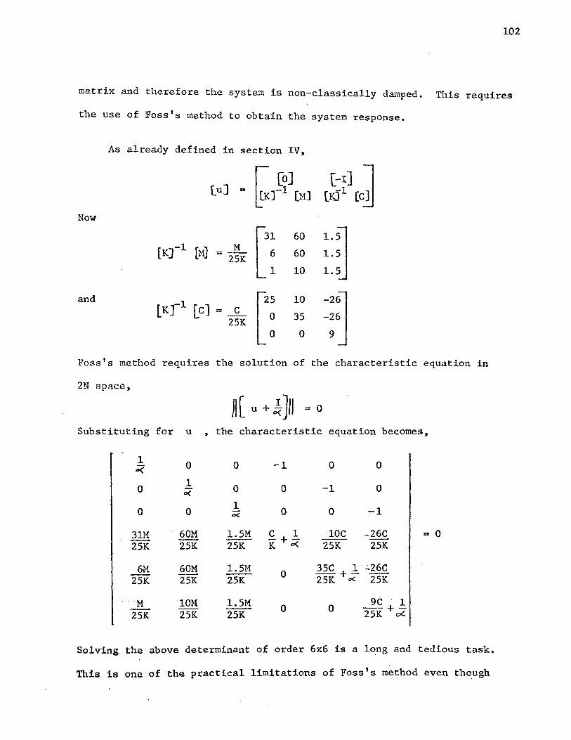
102
matrix and therefore the system is non-classically damped. Titis requires
the use of Foss's method to obtain the system response.
Now
and
As already defined in section IV,
c 25K
60
60
10
1.~ 1.5
1.5
Foss's method requires the solution of the characteristic equation in
2N space,
Jl [ u + ~ ]ll = 0
Substituting for u , the characteristic equation becomes,
1 0 0 -1 0 0 o(
0 1
0 0 -1 0 o(
0 0 1
0 0 -1 oe:
31M 60M 1.5M ~+!. lOC -26C = 0 25K 25K 25K K o< 25K 25K
6M 60M 1.5M 0 35C + !_ -26C
25K 25K 25K 25K o<. 2SK
.. M 10M l.SM 0 0
9C 1 25K 2SK 25K 25K + ~
Solving the above determinant of order 6x6 is a long and tedious task.
This is one of the practical limitations of Foss's method even though
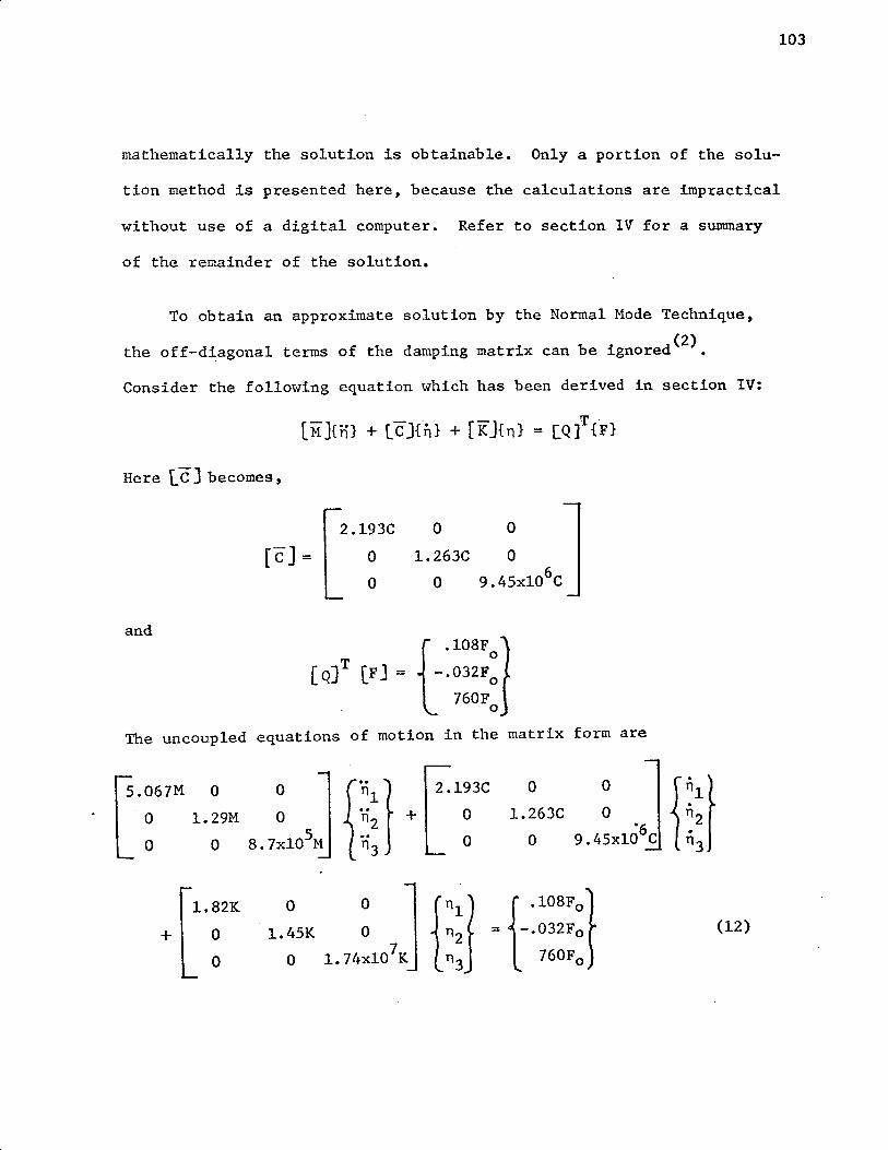
103
mathematically the solution is obtainable. Only a portion of the solu-
tion method is presented here, because the calculations are impractical
without use of a digital computer. Refer to section IV for a summary
of the remainder of the solution.
To obtain an approximate solution by the Normal Mode Technique,
the off-diagonal terms of the damping matrix can be ignored(2).
Consider the following equation which has been derived in section IV:
Here f.. C J becomes,
fc] =
and
2.193C
0
0
0
1.263C
0
( Q) T (F) = -. 032F: {
.108F 1 760F
c 0
The uncoupled equations of motion in the matrix form are
r.067M 0
L ~ 1.~9M
+
1.82K
0
0
0
1.45K
0
2.193C
0
0
0
1.263C
0
0
0 "6
9.45xl0 C
(12)

104
The steady state response is obtained by the equation
(13)
and the phase angle ~i of ni with respect to Fi is given by
(14)
which is a lag angle.
Using equations (13) and (14), the follmving results are obtained
nl = 0.721 ~1 = -28°
n2 = -.702 ~2 = -66.5°
n3 = .00193, ~3 = 49.5°
Using {Xi}= [Q]{ni}' the system response to the harmonic excitation is,
xl = .021 L.:L.
x2 = • s764 L-31. 5°
x3 = 1.564 /84.5°
0 The phase angle of Xi is with respect to X
0(at 0 ). The vector F0
I)
given by equation (4) leads X0 by an angle of 35 • Consequently this
angle is added to ~i (which is with respect to F0 ) to obtain the phase
angle of Xi with respect to X0 •
The damped natural frequency wdi can be calculated by

where wni is the corresponding undamped natural frequency and bi is
the damping ratio, given by
The damped natural frequencies are found to be
wdl = 6.36 rad/sec
wd2 = 10.0 rad/sec
For wd3 ' b3 is greater than one and therefore, the system becomes over
damped. Hence, vibratory motion will not exist in this case.
The system response obtained by approximating the damped system
will be compared later with the exact response obtained by Holzer's
~~thod or by the Impedance Method.
Holzer's Method:
Undamped Free Vibrations: Hith no foundation motion (X=O), the end
support has zero displacement. This is the boundary condition for con-
struction of Holzer table. We shall use the values of the natural
frequencies obtained by the Normal Mode Technique as the trial values
for the Holzer tables.
105

Holzer Table for First Natural
2 .K w = 0.363 M
Mass M Mw2
xi Hw2X LMw2Xi No i 1----
1 M .363K 1.0 .363K .363K
2 10M 3.63K 0.637 2.31K 2.673K
3 l.SM .5445K 0.103 0.056K 2. 73K
-.005
Since the remainder X. = -.005 ~ 0, 1
2 K w1 0.363 M
or w1 = 7.38 rad/sec
Holzer Table for Second Natural Frequency
·Frequency
.Z:Mw2Xi
Ki,i+l Ki,i+l
K .363
5K .534
25K .108
Starting with a trial value of w2 = 1.17 ~ for the second natural
frequency, several trials were made and the corresponding remainder
displacements found. These are tabulated below:
2 Remainder w Amplitude K
1.17 M 0.027
1.16 K 0.0071 M
1.15 K -0.01 M
2 A graph of the remainder displacement versus w is shown on the next
2 page. The points lie on a straight line which crosses w axis at
106

107
0·03
0·0~
0·01 .w ~ <li
m 0 cO
.-i p.. en
•rl to A l·L ~ 1·2. k.. 1-1 2 1"1 M <li w
'1j ~
•rl
~ ~ -o.ot
Figure 19
Remainder Displacement From Holzer's Hethod
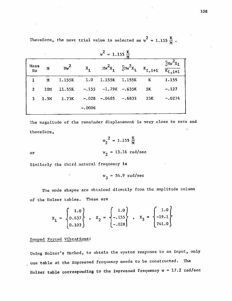
108
Therefore, the next trial value is selected 2 K as w = 1.155 M
2 'K w = 1.155 M
X 2 Mass Mw2 2 LMw2Xi
. Mw Xi M xi Mw X. Ki,i+l No 1 Ki,i+l
1 M 1.155K 1.0 1.155K 1.155K K 1.155
2 10M 11.55K -.155 -1.79K -.635K 5K -.127
3 1.5M 1. 73K -.028 -.0485 -.6835 25K -.0274
-.0006
The magnitude of the remainder displacement is very close to zero and
therefore,
2 K w2 = 1.155 M
or w2 = 13.16 rad/sec
Similarly the third natural frequency is
w3 = 54.9 rad/sec
The mode shapes are obtained directly from the amplitude column
of the Holzer tables. These are
{
1.0} x1 = o.637 ,
0.103 {
1.0} x2
= -.155 ,
-.028 {
l.Of x3
= -19.1
741.0
Damped Forced Vibrations:
Using Holzer's Method, to obtain the system response to an input, only
one·table at the impressed frequency needs to be constructed. The
Holzer table corresponding to the impressed frequency w = 17.2 rad/sec

109
is shown on the next page. For this table, the displacement of the
first mass is assumed to be x1
• The displacements of the remaining masses
are obtained in terms of x1 • The remainder displacement (at the end
support) is then equated to X0
which is 2.0 in. in this case.
From the Holzer table, the displacement at the end support is
(-1.393 + l.i)Xi = 2 (15)
Because of the damping in the system, x1 is a complex number. Let
xl.= a+ ib
Substituting for x1
in equation (15) and rearranging,
(-1.393a- b) + i(a- 1.393b) = 2 (16)
Equating the real and the imaginary parts of the above equation provides
the following two equations:
-1.393a - b = 2
a - 1.393b = 0
which gives
a = -.95
b = -.681
Therefore,
(17)
(18)
* Since the displacements of the remaining masses are in terms of x1 ,
these can be easily calculated. Thus,
* This is obtained from the displacement column of the Holzer table.

Mass Number M Mw2
(1) (2) (3)
1 1 294
2 10 2940
3 1.5 441
w2 = 294
Kj,j+1 xj Mw2xj LMw2Xj +iwC j, j+1
(4) (5) (6) (7)
x1 294X1 294X1 150+1295
.595X1 1750X1 2044X1 750+i2060
+(. 794X1)i +(2330X1)i +(2330X1)i
-.72Xl ·318X1 1726X1 3750+12660
+(1. 30Xl)i +(570X1)i +(2900X1)i
-1. 393X1 +(Xl)i
Holzer Table for an Impressed Frequency of 17.2 rad/sec
Column 6 Column 7
(8)
.405X1
-(. 794X1)i
1.315X1
•(.51X1)i
.673X1 +(.3X1)i
,_. ,_. 0

and
x2 = 1.16/-91.2°
x3 = 1.74 ~25.5°
The phase angles of Xi are relative to the input X0
•
Since there is no approximation involved, the response obtained
above is exact.
For purposes of illustration, a Holzer table to obtain a damped
natural frequency is presented on the next page. Using wd2
obtained
from the first method, as a trial value, the table is constructed as
explained in section V. For a trial value to be a damped natural fre
* quency, the real part of the remainder displacement should be zero •
For w = 10.0 rad/sec, the real part of the remainder displacement is
-.003 v1hich is close to zero and therefore w = 10 rad/sec is one of the
damped natural frequencies of the system.
Impedance Hethod:
In order to apply this method, the various elements of the system are
connected between the points which have been numbered as shown in figure
111
20. Thus across points (1) and (2) are a spring and a damper in parallel
and across points (2) and (3) is a mass, and so on. The velocity v1
at point (1) is wx and the force F1
at this point is unknown. The force
F7
at point (7) is zero as it is a free end. With these boundary con
ditions and knowing the four-pole parameters which relate any two points,
* For detailed explanation, refer to section V.

Mass
Number
(1)
1
2
3
M
(2)
1.0
10.0
1.5
Mw2
(3)
100
1000
150
w2 = 100.0
Xj M\v2xj
(4) (5)
l.O+O.Oi lOO+Oi
.711+.32li 711+32li
.22+.6891 33+103i
-.003+.707i
IMw2xj
(6)
100+0i
811+32li
844+424i
Kj,j+l+iwcm,j+l
(7)
150+171. 3i
750+1200i
3750+1545i
A Holzer Table for a Damped Natural Frequency
Column 6 Column 7
(8)
.289-.32li
.429-.368i
.223-.01761
..... ..... N

4
6'K 7C.
1
Figure 20
A Damped Three Degree-of-freedom System
With Harmonic Excitation
113

the steady state system response can be determined. Using the theory
developed in section VI~ the following relationships are obtained:
[::] = [.oo:l5+i(.oo3o4) :J [::J (19)
[::J = [: 25~8~ J L:: J (20)
[ ::] = ~.00:36+i(.00268) :] [:j (21)
[::] [: 172i Fs J = (22) 1 vs
[::] = [a4:4+(.02~6li :] [:~ (23)
[::] [: 17.2i :J = (24) 1
Applying equation (63) derived in section VI, between points (1)
and (7),
* This is matrix of four-pole parameters of spring K3 and damper c3 which are connected in parallel. For formulas of parallel connections,
refer to section VI.
114

[::] [-5+8.04i = -.0327+.076i
-170+100J [ 0 J -1.4+1.0:1. v
7
Similarly for points (2) and (7),
[:~ L5+8.04i -170+1001] [ 0] = .00246+.074i -. 73+1.31 v7
From equations (25) and (26),
v1 = (-1.4 + l.Oi)V7
and
v7 = -.73 + 1.3li
Substituting for v7
from equation (28) into equation (27) and
simplifying,
vl = 1.15 v2 /25.5:
or v2 = .87 vl /-25.56
or x2 = .87 xl /-25.5°
Now x1 = X0 = 2
Therefore, x2 = 1.74 /-25.5°
which is the displacement vector of M3 •
From equations (19) and (20),
From equation (25),
Fl = (-170 + 100i)V7
115
(25)
(26)
(27)
(28)
(29)
(30)
(31)

Substituting for v7 from equation (28) into equation (31) and
simplifying~
F1 = (113 + 67i)V2
(32)
Substitute the above value of F1 into equation (30), which gives
F3 = (113 + 41.2i)V2
From equations (20) and (21),
(33)
F3
= F4
(35)
V3 = (.00736+.00268i)F4+v4 (36)
Solving equations (33) through (36) simultaneously,
v4 = (.277 - .606i)v2
or x4
= (.277 - .606i)x2
Substituting for x2
in the above equation gives x4 ,
which is the displacement vector of M2•
From equations (24) and (28),
-.73 + 1.3li
x6 = -.73 + 1.3li Xz . or
Substituting for x2
in the above equation,
x6 = 1.163 Dls. s::. which is the displacement vector of M1.
(37)
(38)
116

Expressing the final results in terms of the original system
coordinates,
x1 = 1.163 /215.5°
x2 = 1.16 f-9!':._
x3 = 1.74 ;'-25.5°
These results are in good agreement with those obtained by Holzer's
Method.
yraphical Technique:
For obtaining the steady state system response by this method, define
the coordinates of the system as shown in figure 21. This permits the
direct application of equation (91) derived in section VII.
and
~:here
The individual spring-mass combination frequencies are
w --=
WOl =
W02 =
WQ3 =
w .345, -- = WQ2
50.0 rad/sec
8.66 rad/sec
12.25 rad/sec
w 1.985, -- = W03
w = 17.2 rad/sec
1.4
The ratio of the damping coefficient and the critical damping for
individual M, K, and C is
bl = 1.0, b2 = 0.692, b3 = 0.1
117

Kt
Figure 21
A Damped Three Degree-of-freedom
System With Harmonic Excitation
118

w Corresponding to--- and b., the value of Tdj is read from the dis-woj J
placement transmissibility curve(l, 2). Tfj is then obtained by the
relation
The values of Tdj and Tfj are presented below in a polar notation:
Tdl = 1.1 L!J.o ' Tfl = 0.1 /180°
Td2 = o. n L-6o0
' T£2 = 0.885 /42.4°_
Td3 = 1. 0 /-54° ' T£3 = 0.918M
Using equation (91) of section VII, the amplitude ratios of the
various coordinates can be expressed in terms of Tdj and Tfj by the
following equations:
x2 -= xl
X 0
Equation (39) gives
Td2 [1
x3 -= x2
M3 +-
M2
Td3 (39)
Td3 x rl
Tf Tf2 (1 - _2_) 3 x2
(40)
(41)
1.0 /-s4~ (42)
Equations (40) and (41) can be solved graphically as explained in
section VII. The vector diagram for solving equation (40) is shown
119

on the next page. Thus,
• 72 (_,_Q. = ----~~~~~==~~
1 + .0885 ;-11.6°
= . 72 /-60°. !.086 L-2b_
The value of 1.086 ~2° is obtained from the vector diagram. Thus
(43)
Substituting the numerical values in equation (41) and simplifying,
Expressing the amplitude ratios in terms of the original system
coordinates,
which gives
1.125 t-_21 .6°
. 663 L-58°
1.0 1-st!:_
x3 = 2.25 ;'-27.6°
x2 = 1.49 L-85.6~
(44)
120

121

or
x1 ~ 1.49 /-139.6°
x1 ~ 1.49 /220.4°
TI1e above displacements do not agree with those obtained by Holzer's
Method or by the Impedance Hethod. The discrepancy lies in the ratio
x3 X: . From Holzer's Hethod, 0
whereas by this method,
x3 t - = 0.87-25.5~ xo ~---------
-= X
0
1.125 /--27 .6°
x3 TI1e calculations for Xo were checked and rechecked. However, extensive
investigations failed to provide the desired ratio. The source of
this deviation could not be traced.
The remaining amplitude ratios obtained by the Graphical Technique
are reasonably close to those obtained by Holzer's Method.
Red~ced System:
The impressed frequency w is 17.2 rad/sec and the individual springo
mass combination frequencies are
wnl = 12.25, wn2 = 8.66, wn3 = 50.0
According to the theory presented in section VIII, M3 and c3
should
be eliminated. The reduced system is shown in figure 23.
122

1
150 . 17.13
10
. 12.0
Figure 23
Initial Reduction of the Original System
The above figure is equivalent to the system shown below,
1
150
10
610
Xo·Sin 17.2t
Figure 24
Reduced Two Iegrees-of-freedom System
123

Undamped Free Vibrations: Us~ng Holzer 1 s Method, the following
undamped natural frequencies and the corresponding mode shapes are
obtained-:
wl = 7.25 rad/sec, xl ~ { 1.0} .65
w2 = 13.16 rad/sec, x2 t-0 } = -.155
These results are close to the exact solution obtained by Holzer's
Hethod.
Damped Forced Vibrations: To obtain the response of the reduced system
to the harmonic excitation, a Holzer's table similar to the one pre-
sented for the exact solution is constructed. This table appears on
the next page.
Equating the remainder displacement to X0
gives two simultaneous
equations. TI1us,
-(.715)(a + ib) + il.394(a + ib) = 2
where x1 = a + ib
As before, the real and the imaginary parts of the above equation are
equated which gives
a = -.583, b = -1.13
Therefore,
x1 == 1.27/242.8~
Substituting for x1
in the expression for X2 (obtained from the dis
placement column of the Holzer's table),
124

Mass Number M
(1) (2)
1 1
2 10
w2 = 294.0
K· '+1 Mw2 J,J
Xj piw2xj Mw2Xj +iwC. '+1 J,J (3) (4) (5) (6) (7)
294 x1 294X1 294X1 150+i295
2940 595Xl 1750Xl 2044X1 610+i2060 +(. 794Xl) i +(2330X1)i +(2330X1)i
-.715Xl
+(1. 394X1) i
Holzer Table for Impressed Frequency of 17.2 rad/sec
Column 6 Column 7
(8)
.405X1 -(. 794Xl)i
1.31X1 -(.6X1)i
..... N VI

126
x2 = 1.266 /-64°
The magnitudes of the displacements of the masses are reasonably close
to the exact system response. However, the phase angles of the displace-
ment vectors are in considerable error. An interesting point is that
xl the ratio for obtained by the actual solution as well as by reducing Xz the system is same.
It should be pointed out that approximating the system by ignoring
the off-diagonal terms of the damping matrix can result in serious
error. This is the case for this problem as can be observed by comparing
the exact solution and the approximate solution. For a discussion on
comparison of various methods, the reader is referred to section IX.
The final results obtained by various methods are presented in a tabular
form on the next page.

Method Natural Mode Shapes Amplitude Ratios Frequency (Undamped) (Forced)
Normal 7.38 l.Lo • 637 .10~ • 782 L84. so
Mode 13.2S (1.0 -.17 -. 0321 .368 L-11~ S4.9 u.o -19.1 76~ .036 L38.5~
** 7.38 L!_.o .637 .1~ .87 f2s. S0
Holzer 13.16 lJ.. 0 -.lSS -.02~ .• 666 /-65.7°
S4.9 L!.:o -19.1 741_J 1.06 /-s3. 2°
• 87 L-2s. s:_
Impedance * * .666 L-6S.5°_
1.02 L-53. s__o
1.125 (_-21. Go_
Graphical * * . 663 0£_ 1.0 /-54°
Reduced 7.25 L::o .65J
System 13.16 ~0 ~.15j
1.0 /-53. 2o__
Comparison of Results Obtained EY_ Various Methods
*~fhesc ratios are for the approximate system obtained by ignoring the off-diagonal terms of the damping matrix.
*Values cannot be determined.
127

128
For the above table, the natural frequencies and the mode shapes are
listed in the serial order. Amplitude ratios are in the following
order:

129
VITA
Brij. R. Mohta was born on February 22, 1942, in Bikaner, India.
He graduated from M. V. High School, Bombay, India, in June 1958. He
received a B.S. in Physics and a B.S. in Mechanical Engineering from the
University of Bombay and the School of Mines and Metallurgy (now the
University of Missouri at Rolla) in June 1962 and May 1964 respectively.
Immediately thereafter he was employed by Voltas Limited, Bombay,
in the Earthmoving and Mining Division. He attained the position of
Senior Engineer - Sales before leaving Voltas in December 1966.
He has been enrolled in the Graduate School of the University of
Missouri at Rolla since January 1967.